Embed Size (px)
Citation preview

Solar Energy 74 (2003) 157–173
C omparison between ray-tracing simulations and bi-directionaltransmission measurements on prismatic glazing
a , b a*Marilyne Andersen , Michael Rubin , Jean-Louis ScartezziniaSolar Energy and Building Physics Laboratory LESO-PB, Swiss Federal Institute of Technology EPFL, 1015 Lausanne, Switzerland
bLawrence Berkeley National Laboratory, University of California, 1 Cyclotron Road, MS 2-300, Berkeley, CA 94720-8134,USA
Abstract
Evaluation of solar heat gain and daylight distribution through complex window and shading systems requires thedetermination of the bi-directional transmission distribution function (BTDF). Measurement of BTDF can be time-consuming, and inaccuracies are likely because of physical constraints and experimental adjustments. A general calculationmethodology, based on more easily measurable component properties, would be preferable and would allow much moreflexibility. In this paper, measurements and calculations are compared for the specific case of prismatic daylight-redirectingpanels. Measurements were performed in a photogoniometer equipped with a digital-imaging detection system. A virtualcopy of the photogoniometer was then constructed with commercial ray-tracing software. For the first time, an attempt ismade to validate detailed bi-directional properties for a complex system by comparing an extensive set of experimentalBTDF data with ray-tracing calculations. The results generally agree under a range of input and output angles to a degreeadequate for evaluation of glazing systems. An analysis is presented to show that the simultaneously measured diffuse anddirect components of light transmitted by the panel are properly represented. Calculations were also performed using a morerealistic model of the source and ideal model of the detector. Deviations from the photogoniometer model were small and theresults were similar in form. Despite the lack of an absolute measurement standard, the good agreement in results promotesconfidence in both the photogoniometer and in the calculation method.Published by Elsevier Science Ltd.
1 . Introduction Breitenbach and Rosenfeld, 1998; Aydinli, 1999). Theoperating principle of the photogoniometer developed at
Energy savings objectives and improvement of visual the LESO-PB/EPFL is different: it is based on thecomfort in buildings has led to a growing need for accurate observation of a mobile projection screen, from which thebi-directional transmission data for advanced windows, transmitted light is reflected into a calibrated CCD camerashading systems and daylight redirecting devices. Special- (Andersen et al., 2001). This technique allows a consider-ized experimental systems have been developed to measure able reduction of the time needed to perform BTDFthe bi-directional (light) distribution function. This BTDF measurements. The entire light distribution is characterizedfunction is defined as ‘the quotient of the luminance of a within six screen rotations instead of hundreds or moresurface element in a given direction, by the illuminance likely thousands of detector movements through a compar-incident on the sample’ (CIE, 1977), and is expressed in able number of positions. Also, this approach gives
22 21 21[cd m lx ] or [sr ]. continuous knowledge of the whole transmission space,The usual way to measure bi-directional transmission averaged into finite zones, instead of discrete transmission
functions is based on a point-per-point mapping of the assessments that need to be interpolated.emerging hemisphere with a device-specific detector There is however a lack of standards for absolute(Papamichael et al., 1988; Murray-Coleman and Smith, determination of the optical properties of complex glazing1990; Apian-Bennewitz, 1994; Bakker and van Dijk, 1995; systems. Consequently, validation of BTDF data obtained
with photogoniometric measurements has so far beenrestricted to two limited possibilities: (a) perform BTDF*Corresponding author. Tel.:141-21-693-4551; fax:141-21-measurements on simple glazing or systems, which can be693-2722.
E-mail address: [email protected](M. Andersen). assessed in a standardized spectrometer or analytically
0038-092X/03/$ – see front matter Published by Elsevier Science Ltd.doi:10.1016/S0038-092X(03)00115-4
158 M. Andersen et al. / Solar Energy 74 (2003) 157–173
Nomenclature
(u , f ) polar co-ordinates of incoming light flux (8)1 1
(u , f ) polar co-ordinates of emerging (transmitted) light flux (8)2 2
r reflection factor of projection screen (–)d distance from sample center to screen along direction (u , f ) (m)2 2
2A illuminated area of sample (m )a angle between normal to screen and direction (u , f ) (8)2 2
22L (u , f , u , f ) luminance of the projection screen area associated to the direction (u , f ) (cd m )screen 1 1 2 2 2 2
E (u ) illuminance of the fenestration material due to the incoming light flux (lx).1 1
Du , Df output angular resolution (8)2 2
F incoming flux along direction (u , f ) (lumen)1 1 1
F transmitted flux along direction (u , f ) (lumen)2 2 2
F transmitted flux along direction (u , f ) normalized to incident flux (–)2norm 2 2
d detection hemisphere radius (distance from sample center to ideal detection surface) (m)hemis
t(u , f ) hemispherical light transmittance of sample under incident direction (u , f ) (–)1 1 1 122L luminance of incoming light flux (cd m )1
22L luminance of emerging (transmitted) light flux (cd m )2
V solid angle subtended by incident light flux (sr)1
V solid angle subtended by emerging (transmitted) light flux (sr)2
h distance from sample center to light source (m)L luminance emitted from the projection screen, due to direct (specular) transmissionscreen spec
] 22(cd m )22L luminance emitted from the projection screen, due to diffuse transmission (cd m )screen diff
] 2A area of source that emits rays towards the sample (m )source2A area considered on the screen for emerging (transmitted) light detection (m )screen
calculated (Murray-Coleman and Smith, 1990; Andersen et However, they have so far never served extensively as aal., 2000); (b) calculate the global transmittance values basis for BTDF measurement comparisons, as presentedfrom an integration of BTDFs over the emerging hemi- here.sphere and compare them to Ulbricht sphere measurements In this paper, experimental conditions for BTDF charac-(Murray-Coleman and Smith, 1990; Apian-Bennewitz, terization with the digital imaging-based photogoniometer1994; Breitenbach and Rosenfeld, 1998; Andersen et al., developed at the Swiss Federal Institute of Technology2000; van Dijk, 2001). These methods are reliable, and (EPFL) are reproduced virtually with the commercial
1obtaining good results in such comparisons is promising forward ray-tracer TRACEPRO for two acrylic prismaticfor the BTDF assessment accuracy. However, they cannot panels. The latter have been chosen as a validationbe considered as sufficient to prove that individual BTDF example because they consist of a material of well-knownvalues are accurate enough for fenestration systems of refraction coefficients, thus easily handled by the softwarearbitrary complexity. Likewise, a BTDF comparison from applying Snell–Descartes’ law, whereas at the same timeone facility to another cannot provide definitive conclu- they present complex transmission features because of thesions yet, as neither of the two datasets could be consid- multiple inside reflections and interactions between theered as better than the other. gratings.
The use of ray-tracing techniques can provide a generalmethod for evaluating complex systems in full detail andadd a point of comparison to bi-directional measurements. 2 . Description of BTDF experimental assessmentThe combination of experimental and computational meth- methodods will increase flexibility and efficiency by restricting theexperimental part to the essential measurements only, i.e. The principle of the bi-directional photogoniometerthe transmission and reflection properties of unknown constructed at the Solar Energy and Building Physicscomponent coatings or materials. Computational methods Laboratory (LESO-PB/EPFL) is based on digital imaginghave already been used or developed for the assessment of techniques. The light transmitted from the sample iscomplex glazing (see e.g.Compagnon, 1994; Mitanchey et reflected by a diffusing triangular panel towards a charge-al., 1995; Molina et al., 1995; Campbell, 1998; Kuhn et al.,
1 2000), and have proven their usefulness and potentialities. TRACEPRO , v. 2.3 & 2.4, Lambda Research Corporation.

M. Andersen et al. / Solar Energy 74 (2003) 157–173 159
2 area of the sample (m );a is the angle between the normalto the screen and the direction (u , f ) (8); L (u , f ,2 2 screen 1 1
u , f ) is the luminance of the projection screen area2 222associated to the direction (u , f ) (cd m ); E (u ) is the2 2 1 1
illuminance of the fenestration material due to the incom-ing light flux (lx).
In order to determine BTDF values according to aregular output resolution (Du , Df ), outgoing zones have2 2
to be defined around the considered directions (u , f ).2 2
The luminances due to the transmitted light flux beingmeasured on a projection screen, the latter must be dividedinto a grid of zones depending on the desired outputresolution. The size of the zones (i.e. the number ofcomprised pixels) are hence inversely proportional to thenumber of analysed directions, which are bound to theoutput resolution.
This approach allows the investigation of the wholetransmission hemisphere without any unexplored area.Resolution-dependent BTDF values result from an averageFig. 1. Diagram of the LESO-PB bi-directional photogoniometerover a certain outgoing zone, limited by (f 2 0.5Df ;showing the use of a CCD camera as a multiple-points luminance- 2 2
f 1 0.5Df ) in azimuth and by (u 20.5Du ; u 1meter. 2 2 2 2 2
0.5Du ) in altitude for each outgoing direction. For non-2
Lambertian materials, such BTDF data will thereforecoupled device (CCD) camera, which provides a picture of present differences with point-per-point photogoniometricthe whole screen, as illustrated byFig. 1. The incident measurements, where a new output resolution only affectsdirection (u , f ) is determined by inclining the device the shift between two measurement positions, and not the1 1
(and hence the sample plane) around a horizontal axis at BTDF value itself obtained for a given direction (u , f ).2 2
altitudeu and by rotating the sample around its normal to On the other hand, the conventional method cannot avoid a1
reach azimuthf , the light source remaining fixed. loss of information for the in-between regions. The dis-1
The CCD camera is used as a multiple-points cretization of the output hemisphere into zones represent-luminance-meter, and has been calibrated accordingly ing average light emergence around particular directions(Andersen et al., 2001); a relation between the pixel’s (u , f ) has thus the important advantage of providing a2 2
coordinates on the image and the angular direction (u , f ) continuous characterization of the transmitted light dis-2 2
they correspond to has been established as a function of tribution. This is particularly critical when the latterthe sample thickness and the incident azimuth valuef (as presents narrow luminance peaks as in the case of pris-1
the referential rotates with the sample for non-zero matic panels.azimuthsf ), thanks to the use of matrix calculations Other major advantages of digital-imaging techniques1
(Andersen, 2001). After six 608 rotations of the screen- are the great reduction in time to complete the full set ofcamera system (with image capture, calibration and pro- measurements, and accuracy holding even for high lumi-cessing at each position), the transmitted light distribution nance dynamics.is fully known. ‘Screen’ luminance values can then be It must be noted that this assessment method leads toconverted into BTDF data according to Eq. (1), where BTDF average values not only related to the direction ofdistance and light tilting effects are compensated. Details the emerging rays, but also to the angular areas wherecan be found inAndersen et al. (2001)and Andersen these rays are detected, whose location is determined by(2002). the considered direction and its size by the output res-
olution. This difference has however a negligible impact2d (u ,f )cd p 2 2 on the monitored data as long as the distance from the]] ] ]]]]BTDF(u ,f ,u ,f ) 5 ?F G1 1 2 2 2 r A ? cosu ? cosam lx 2 sample to the detector (screen) is large compared to thesample size, a factor of 10 being accepted as reasonable.L (u ,f ,u ,f )screen 1 1 2 2
]]]]]]? (1) Besides, the angular resolution is always chosen accordingE (u )1 1to the sample size, in order to remain consistent with thepossible divergence of rays reaching a given point.where (u , f ) are the polar co-ordinates of incoming light1 1
Experimental assessment of BTDFs and correspondingflux (8); (u , f ) are the polar co-ordinates of emerging2 2
ray-tracing calculations were compared for prismatic(transmitted) light flux (8); r is the reflection factor of thepanels, revealing a specular transmission with directionalprojection screen (–);d is the distance from sample centerchanges due to refraction. Formally, a BTDF is onlyto screen along direction (u , f ) (m); A is the illuminated2 2

160 M. Andersen et al. / Solar Energy 74 (2003) 157–173
defined for diffuse transmission (CIE, 1977); however, as program, acrylic being a common material with well-pointed out byMurray-Coleman and Smith (1990),BTDFs known wavelength-dependent indices of refraction. At theare capable of describing specular as well as diffuse same time, they present complex transmission featurestransmission. In the specular case, BTDFs present a finite because of the multiple internal reflections and interactionsvalue determined by the incident angle, the transmittance, between adjacent gratings.and the source solid angle, except in the limit of a The dimensions of the two panels are, respectively:vanishingly small source solid angle, where a specular height (vertical dimension) 90 mm, length (horizontalBTDF will approach infinity. Although the analytical dimension) 200 mm and thickness 12 mm for the symmet-expressions of BTDFs differ whether they are related to ric panel (height of individual grating515 mm); heightspecular or diffuse light, their common assessment can be 195 mm, length 200 mm and thickness 12 mm for theaccepted under certain conditions, presented in Appendix asymmetric panel (height of individual grating57 mm, lastA. These conditions can be considered as reasonably grating incomplete).approached for the particular data acquisition methodology The origin of the co-ordinate system is placed on thedeveloped for the formerly described digital imaging-based panel (seeFig. 3). Directions are defined by sphericalphotogoniometer, as detailed in Appendix A and shown by co-ordinates: altitude angleu comprised between 08 andi
the ideal situation comparison exposed in Section 6. 908, and azimuth anglef comprised between 08 and 3608,i
where indexi indicates whether it is related to the incident(i 5 1) or transmitted (i 5 2) direction. The respective baseplanes are the external (on incidence side) and internal (on
3 . Characterization parameters and sample emerging side) sample interfaces.description A full set of BTDF data was generated experimentally
for the symmetric panel (with flat face on incident side),Two acrylic prismatic panels, manufactured by Siemens, according to the 145 incident directions of the sky lumi-
have been selected for this study among the samples nance mapping proposed byTregenza (1987)within thecharacterized with the bi-directional photogoniometer: one IDMP international programme; this set is considered as apresents symmetric gratings of slope 458 (seeFig. 2A) and standard for photogoniometric data at the internationalthe other asymmetric gratings of slope 428 and 58 (Fig. level (Aydinli, 1999). The maximum set of incident2B). These particular complex glazing materials were directions has been reduced because of the samplechosen because of their combination of simplicity in symmetries, leading to 42 relevant incident directions forvirtual representation and complexity in light transmission. the 458 gratings panel. This sample was characterized forTheir geometric characteristics are well defined and can be six additional incident directions, defined by:u 5208 and1
determined at a macroscopic level. In addition, their 408, f 5 08, 458 and 908.1
physical properties can be easily described in a simulation The asymmetric panel was analysed for gratings on both
Fig. 2. Section view and parallel perspective of the prismatic panels used for BTDF assessment validation. (A) Symmetric panel, gratings458. (B) Asymmetric panel, gratings 428 and 58.

M. Andersen et al. / Solar Energy 74 (2003) 157–173 161
Fig. 3. Spatial referential with regard to the sample orientation for incident (index 1) and transmitted (index 2) directions.
incident and emerging sides (the 58 slope upwards, as in The detection screen is a triangle of base 115 cm andFig. 2B), and along azimuthal planesf 508, 908 and 2708 height 152.1 cm, fixed on a rotating ring with an angle of1
with a regular altitude increment of 108. 49.18 (5atan 2/œ3) in order that its projection on theThe light source consists of a HMI 2.5 kW discharge sample plane represents an equilateral triangle. Its base
lamp with a Fresnel lens. Its spectrum is given inFig. 4; as plane is slightly shifted out from the incident base planedetailed inAndersen et al. (2000),the uniformity of the (7.5 cm between the two).incident radiation has been checked to present a relative The output resolution is equal for both samples (Du 52
mean deviation lower than 1.8% over the sample area, and 58, Df 558). Because of the samples’ physical dimen-2
the analysis of the collimation of the beam reaching the sion, the illuminated area for the symmetric panel waslatter has led to a half angle of 0.48. restricted to a disk of diameter 6 cm with an opaque
Fig. 4. Relative spectrum for the real incident source (HMI 2.5 kW discharge lamp mounted with Fresnel lens), and approximation by stepfunction for a discrete wavelength set.

162 M. Andersen et al. / Solar Energy 74 (2003) 157–173
diaphragm, whereas the asymmetric panel was measured mation as a step function presenting five different levels. Inwith a 10 cm diaphragm. order to define a (discrete) list of wavelengths to be traced
that would be representative of the incident source spec-trum, each wavelength interval determined by the stepfunction is associated to a number of wavelengths to be4 . Virtual reproduction of BTDF measurements withconsidered within the particular interval, proportional toray-tracing calculationsthe latter’s width and to the source spectrum amplitude,and given inFig. 4 as well. The set of wavelengths to beIn order to validate the measured BTDF values, the
considered remains quite large and involves substantialcommercial ray-tracing simulation software TRACEPRO ,time consumption for the simulation. A reduction by abased on Monte Carlo calculations, was used to replicatefactor of 4 was shown not to affect the results significantlythe experimental conditions. All the optical components(differences lower than 2%).(light source, spectrum, sample, detection system) were
Instead of either moving the sample and detectortherefore simulated with geometric and material charac-according to the incidence angles, or the source itself, ateristics as close as possible to the reality. Of course, thevirtual source was placed against the outside samplevirtual BTDF values are ideal in regards to what theinterface fitting the experimental sample diaphragm aper-experimental set-up can generate: in addition to theture (illuminated area), with rays emitted at varying anglesinevitable uncertainties due to the components’ physical(direction vectors) depending on the incident directionnature, the model was built according to the simplificationconsidered.hypotheses formulated byCompagnon (1994),neglecting
The prismatic elements were modelled according to theirlight dispersion and absorption inside the prismatic materi-real geometric features (even though ideal because as-al, edge effects or dust, and shape imperfections (likesumed of perfect shape). Thanks to a combination ofrounded grating edges appearing for any manufacturedprimitive solids creation and subtractive or additive toolselement). These simplifications were nevertheless taken proposed by TRACEPRO , the respective gratings of 458into account within the error calculation procedure (seeslope and, with more complexity, 428 and 58 slopes wereSection 5).built (see Fig. 2). The elements were modelled as anThe simulation model needs to follow important con-acrylic material, according to the software’s database ofstraints, such as:refractive indices (provided by the manufacturers).• the incident source must be of the same angular spread
An opaque (100% absorbing) diaphragm of apertureas the real one; a set of wavelengths representative of
diameter, respectively, 6 cm and 10 cm for the symmetricits spectrum has to be determined; the source has to be
and asymmetric panels was placed in front of the incidentpositioned in order to reproduce the same incident
sample interface. An additional surface, presenting nodirections as the ones analysed;
interaction whatsoever with its environment, was created• a sample of same geometric and physical (acrylic)between the diaphragm and the sample in order to normal-
properties as the one measured has to be modelled; theize light flux calculations with a reference value.
sample area exposed to light has to fit the illuminatedThe current software features do not allow a spatial
surface during experimental characterization;investigation of an object according to angular parameters.• a detection screen of the same geometry as the one usedInstead, a set of individual detectors, associated to the
physically for the measurement facility and separateddifferent zones, was created. Practically, in order to have
into the same pattern of zones (solid angles aroundonly one tracing session (and not six), all the six screen
outgoing directions, see Section 2) has to be modelled.positions were simulated at once by way of six virtual
For each prismatic panel, five representative incidences screens in the simulation model. Each screen is split intowere selected amongst the full set of 98 incident directions zones using planes of azimuths 08, 58, etc. and cones ofthat were characterized experimentally. The corresponding half angles 2.58, 7.58, etc. which determine the intersectionangular couples (u , f ) are: for the symmetric panel (flat1 1 lines of the zones. With an output resolution (Du , Df )2 2face on incident side), (408, 908), (608, 908), (248, 308), equal to (58, 58), about 1400 different reception surfaces(408, 458) and (608, 758); for the asymmetric panel, (208, were created.08) and (408, 908) for the flat face on incident side, (08, 08), As explained in Section 4.2, the observed quantity is the(108, 908) and (208, 2708) for the gratings on the incident total photometric flux received by each detection zone,side. easily convertible into the corresponding BTDF value
through Eq. (2). There is therefore no need to model the4 .1. Virtual components reflection on a diffusing screen and the detection by the
CCD camera, the calculation results being already compar-The spectrum of the incident source is given inFig. 4 able to experimental data. Furthermore, detecting the
over the visible wavelength range (380 through 780 nm); transmitted light directly on the screen allows an accuratethe continuous curve is shown together with its approxi- estimation of the measurement error induced by the

M. Andersen et al. / Solar Energy 74 (2003) 157–173 163
camera’s calibration procedures (spectral, photometric, the normalized fluxF (%) coming out from the2norm
geometric, additional corrections). To avoid inter-reflec- sample and reaching a discretization zone on the screentions between the different detection surfaces, they were (i.e. emitted into the solid angleV (sr) determined by the2
defined as perfect absorbers in the simulation model; they outgoing direction (u , f ) and the resolution (Du , Df )).2 2 2 2
are shown inFig. 5 together with the prismatic panel and The BTDF being defined as the quotient of the luminancethe opaque diaphragm. of a surface element in a given direction by the illumi-
nance incident on the sample, these fluxes can be con-4 .2. Ray-tracing results and conversion into BTDF verted into the associated BTDF values through Eq. (2),values the differential quantities being approximated by their
equivalent average values (Murray-Coleman and Smith,The rays were emitted from an annular grid, composed 1990):
of 45 rings and sending about 200,000 rays (|6000 rays atL F A2 221each wavelength). The flux threshold (fractional value of ] ]]] ]BTDF(u ,f ,u ,f ) [sr ]5 5 ?1 1 2 2 E FV A cosu1 12 2starting flux for which a ray will be terminated) was set to
0.05. It was checked that a larger number of rays (e.g. F [%]2norm]]]]]]5 (2)15,000 per wavelength) or a lower cut-off value (e.g. Du ?Df ? sinu ? cosu2 2 2 2
0.001) did not significantly affect the results: both induced22where L (cd m ) is the luminance of the emergingdifferences lower than 1% whereas computer simulation 2
(transmitted) light fluxF ; Du and Df are expressedtime was considerably increased. 2 2 2
here in radians.A Lambertian spread of 0.48 (half angle) was applied toOnce converted into the corresponding BTDF values,the beam for the symmetric and asymmetric panels,
the angles (u , f ) being the ones to which the zone isaccording to the incident source collimation characteristics 2 2
assigned, the data can be compared to the experimentalfor the experimental set-up (see Section 3). It must beBTDF values. Both experimental and simulated BTDFnoted that the source does not appear as a separate objectvalues are assessed here inside a certain angular areain the model: it sends rays according to particular grid andaround the associated couples (u , f ), and thus depend onbeam specifications, but has no physical (optical) prop- 2 2
the output resolution (Du , Df ).They represent averageerties. 2 2
values of BTDFs inside these areas, and provide a continu-As explained above, the analysed quantitative output isous—thus complete—investigation of the transmitted lightdistribution, unlike point-per-point data that represent
particular BTDF values along specific directions (u , f ).2 2
5 . Results comparison
The simulated light flux was detected in each discretiza-tion zone, converted in photometric units (lumens) andnormalized to the incident flux. As the transmissionfeatures are very sharp (and therefore cover only smallsolid angles), the discrepancies between real and virtualvalues can be revealed by two-dimensional plots forvarying altitudesu and along given azimuthsf , which2 2
allows to point out differences with high accuracy.The results are shown inFigs. 6–11with an output
resolution (Du , Df ) of (58, 58). For each analysed2 2
situation, the relevant outgoing azimuthal planes (i.e. theanglesf for which the transmission is non-zero) were2
determined. Both measured and calculated BTDF datawere reported along these outgoing planes as functions ofaltitudeu for the 10 selected incident directions. For the2
symmetric panel (gratings 458, flat face on incident side)these incident directions were (408, 908), (608, 908), (248,308), (408, 458) and (608, 758). For the asymmetric panelFig. 5. Simulation model composed of an opaque diaphragm, thethe incident directions were (208, 08), (408, 908), (08, 08),considered prismatic panel (sample), a non-interacting incident(108, 908) and (208, 2708), the first two being investigatedflux detection surface and six absorbing detection screens split
into angular zones of spread (Du , Df )5(58, 58). with the flat face on the incident side, the others with the2 2

164 M. Andersen et al. / Solar Energy 74 (2003) 157–173
21Fig. 6. BTDF (sr ) vs.u (8) alongf planes: comparison of measurements (BTDFmeas) and calculations (BTDFsim) for the symmetric2 2
panel (slope 458, flat face on incident side) under incidence (408, 908). (A) Main section view, along planef 52708. (B, C) Azimuth planes2
next to the main one, forf 5 2658 and 2758.2
428, 58 gratings on the incident side. The azimuthal planes having significant differences between two assessmentnext to the most relevant ones were also checked (planes methods), low discrepancies and a similar qualitative lightf 6Df andf 62Df , wheref is the azimuth angle for behaviour can be observed, the peaks corresponding2 2 2 2 2
which the BTDFs reached their highest values) and exactly to the same directions, for the main as well as thegenerally revealed the same kinds of behaviours as the secondary maxima.main plane, as shown inFigs. 6 and 10. The error bars given in all the figures for the experimen-
A good agreement between the real and virtual BTDF tal and computational BTDF data are equal to 13% andvalues is achieved. Even though the transmission features 10%, respectively, in relative terms.are extremely sharp (high gradients increase the risk of Uncertainties due to the CCD camera calibration pro-
21Fig. 7. BTDF (sr ) vs.u (8) alongf planes: comparison of measurements (BTDFmeas) and calculations (BTDFsim) for the symmetric2 2
panel (slope 458, flat face on incident side). (A) Incidence (608, 908), main section view. (B) Incidence (248, 308), main peak.
M. Andersen et al. / Solar Energy 74 (2003) 157–173 165
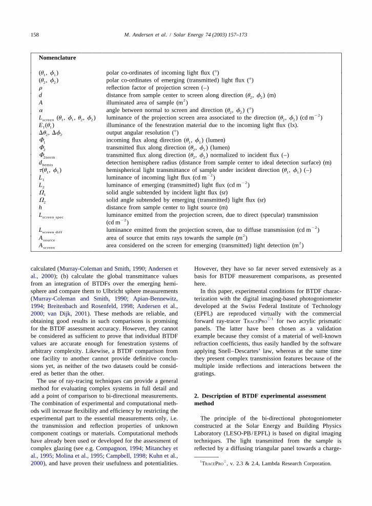
21Fig. 8. BTDF (sr ) vs.u (8) alongf planes: comparison of measurements (BTDFmeas) and calculations (BTDFsim) for the symmetric2 2
panel (slope 458, flat face on incident side). (A) Incidence (408, 458), main peak. (B) Incidence (608, 758), main and secondary peaks.
cedures and other corrections have been investigated of the simplification hypotheses in the prism modellingthoroughly inAndersen et al. (2000);their impact on the (see Section 4), which was assessed by changing slightlyBTDFs is 5%. The discrepancies connected to the spatial some simulation parameters and examining how theseadjustment of the facility components have been added, changes affected the BTDF data. Several altered modelsestimated by modelling slight variations (60.58, 62 mm) were created for both panels and each modification wasin the incident direction or detection screen position and analysed individually:observing the effect on the final results, which is of 8%. • acrylic refraction indices (close to 1.49 over most of theThis led to a global error of 13% for the measurements. visible spectrum) slightly changed (average differenceThe 10% relative error for the model includes the impact of 0.01);
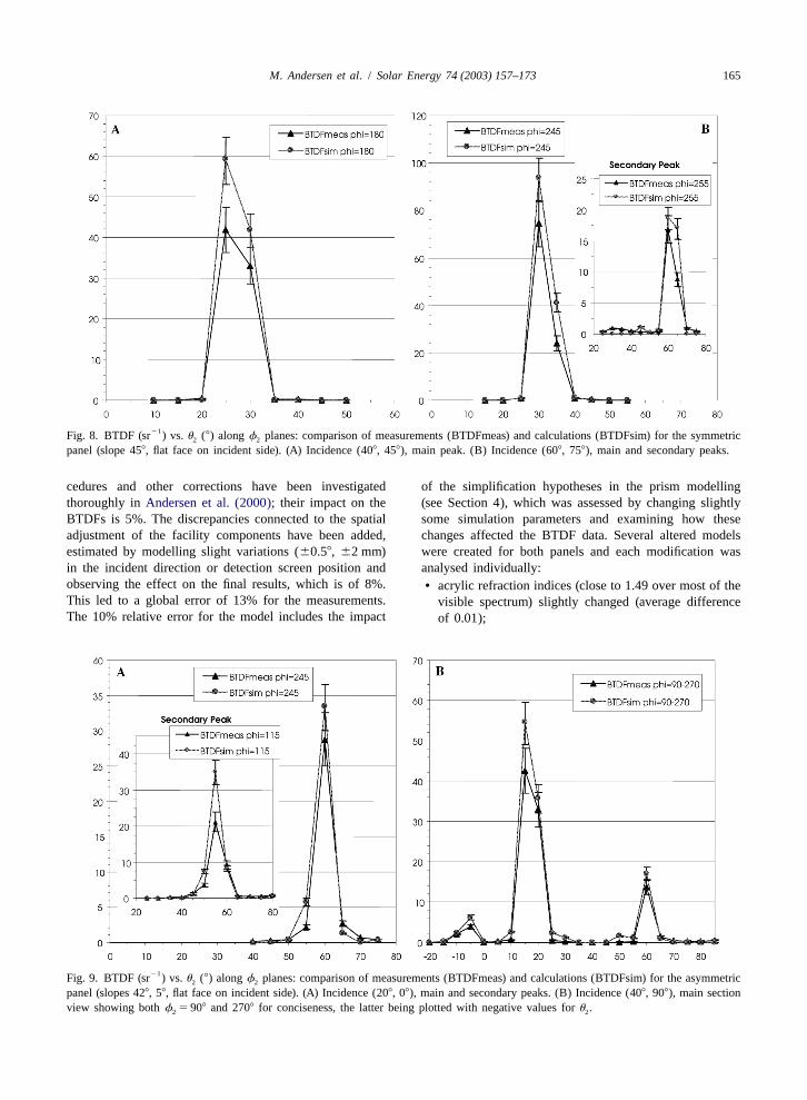
21Fig. 9. BTDF (sr ) vs.u (8) alongf planes: comparison of measurements (BTDFmeas) and calculations (BTDFsim) for the asymmetric2 2
panel (slopes 428, 58, flat face on incident side). (A) Incidence (208, 08), main and secondary peaks. (B) Incidence (408, 908), main sectionview showing bothf 5908 and 2708 for conciseness, the latter being plotted with negative values foru .2 2
166 M. Andersen et al. / Solar Energy 74 (2003) 157–173
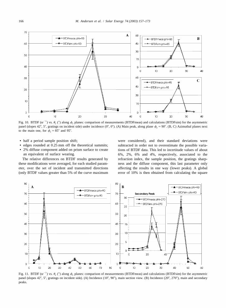
21Fig. 10. BTDF (sr ) vs.u (8) alongf planes: comparison of measurements (BTDFmeas) and calculations (BTDFsim) for the asymmetric2 2
panel (slopes 428, 58, gratings on incident side) under incidence (08, 08). (A) Main peak, along planef 5908. (B, C) Azimuthal planes next2
to the main one, forf 5 858 and 958.2
• half a period sample position shift; were considered), and their standard deviations were• edges rounded at 0.25 mm off the theoretical summits; subtracted in order not to overestimate the possible varia-• 2% diffuse component added on prism surface to create tions of BTDF data. This led to incertitude values of about
an equivalent of surface wearing. 6%, 2%, 6% and 4%, respectively, associated to theThe relative differences on BTDF results generated by refraction index, the sample position, the gratings sharp-
these modifications were averaged, for each studied param- ness and the diffuse component, this last parameter onlyeter, over the set of incident and transmitted directions affecting the results in one way (lower peaks). A global(only BTDF values greater than 5% of the curve maximum error of 10% is then obtained from calculating the square
21Fig. 11. BTDF (sr ) vs.u (8) alongf planes: comparison of measurements (BTDFmeas) and calculations (BTDFsim) for the asymmetric2 2
panel (slopes 428, 58, gratings on incident side). (A) Incidence (108, 908), main section view. (B) Incidence (208, 2708), main and secondarypeaks.

M. Andersen et al. / Solar Energy 74 (2003) 157–173 167
root of the sum of the squared individual relative ince- The parameterisation of a virtual sun is realized byrtitudes, including the ones due to the chosen values of approximating its continuous spectrum with a discrete set
threshold, number of emitted rays and the source spectrum of values, given inFig. 12. A new TRACEPRO versiondiscretization, mentioned in Section 4. having been released in the meantime, the wavelength set
Figs. 6–11make up a positive reciprocal validation, on does not have to account for the right number of wave-one hand of the detection technique and the calibration and lengths to be simulated inside each interval to represent thecorrection procedures, and on the other hand of the spectrum (see Section 4.1); individual wavelength valuesreliability and applicability of ray-tracing calculations for to which weights are assigned are used instead, propor-complex glazing assessment. tional to the associated radiance value. The rays are
emitted according to a Lambertian distribution presentingan angular spread of 0.258.
6 . Simulation of ideal experimental conditions As far as the detection surface is concerned, even thougha flat projection screen is preferable to avoid any risk of
Experimental BTDF data have been verified by re- inter-reflection, a virtual hemispherical surface discretizedproducing the measurement conditions as faithfully as in the same way makes up a more ideal detection surface,possible with the simulation program, in order to estimate the light being collected at a constant distance from thethe error due to the detection technique, i.e. to the CCD sample and with normal rays. Moreover, as explained incamera calibration procedures (spectral, photometric, Appendix A, if the source is sufficiently far away from theimage uniformity, etc.), the geometric relations determined sample compared to the sample-to-screen distanced (u ,2
between image pixels and actual outgoing directions, and f ) (which is of course the case for the sun), the2
the diffusing quality of the projection screen. The results transmitted light reception surfaceA (or more gener-screen
presented in Section 5 show that these essential procedures allyA cosa for surfaces that would not be normal toscreen
seem to be appropriate and that the results assessed thanks the rays) has to be comparable to the apparent illuminatedto this digital imaging-based methodology are reliable. area of the sample, i.e. toA cosu .1
To complement this study, an additional analysis ren- AsA is fixed by the diaphragm used during experimen-dered possible by the flexibility in virtual situations was tal characterization, and as the output resolution (Du ,2
carried out: the modelling of an ideal set-up, whose results Df ) must be equal to (58, 58), the only parameter that can2
could be compared to the experimental conditions. be adjusted to fit this condition is the hemisphericalIn our case, the ideal light source would of course be the detector’s radiusd (distance to hemisphere). Ofhemis
sun itself, whose particular spectrum is given inFig. 12 in course, the (58, 58) discretization zone surfaces vary over2relative values over the visible range, and whose collima- the hemisphere according tod sin u Du Df , wherehemis 2 2 2
tion is almost perfect (half-angle 0.258). Du andDf are both equal to 0.0873 rad; the calculation2 2
Fig. 12. Relative solar spectrum and approximation by a set of discrete values at regular wavelength intervals, providing the weights to beassigned to each considered wavelength.

168 M. Andersen et al. / Solar Energy 74 (2003) 157–173
of d for the 6 and the 10 cm diaphragm diameters is peaks are distributed on a small number of angular zones,hemis
therefore done by taking the average discretization zone only some of the zones have been created on the hemis-surface over the whole hemisphere, and the obtained radii pherical detector, in order to facilitate their assignment toare, respectively, 53.5 and 89.1 cm. These values hence the corresponding angular couples (u , f ).2 2
provide the distance at which the detection surfaces should The simulation model is shown inFig. 13 with thebe positioned for an ideal BTDF characterization with traced rays for the asymmetric panel, incidence (408, 908).specular transmission of the symmetric and asymmetric Towards the left appears the reflected part of the incidentpanels, according to an output resolution of 58 in both beam, not considered in this study. The figure clearlyaltitude and azimuth. It must be observed that for the outlines the spread of transmitted rays induced by thedefault sample diaphragm diameter (10 cm), the hemi- variation of the refractive index with the wavelength, alsosphere radius is extremely close to the actual average observed for the other incidence directions (and for thedistance from the sample to the projection screen in the experimental conditions model). The transmission peaks,experimental facility, equal to 90.5 cm. As mentioned in revealed byFigs. 6–11 and 14–17, cannot always beSection 2, in order that a surface detection becomes identified on these ray-trace plots. The sensitivity of theequivalent to a directional analysis of rays emerging from human eye (photopic curveV(l)) is taken into account fora non-punctual surface, the distance between the sample photometric flux estimations, assigning varying weights toand the detector should be at least 10 times larger than the rays of different wavelengths. Also, the plots cannotsample diameter, which is about the case for the de- provide quantitative information on the weight of each ray,termined ‘ideal’ hemisphere radii (as well as for the which are all shown in the same way even thoughexperimental set-up). The output referential being linked to representative of very different flux values.the emerging face of the sample, the detection hemisphere The comparison of BTDF values obtained by measure-is modelled with a base plane merged with the latter. ment and by simulation with ideal conditions is given in
The incident directions analysed for this study are (408, Figs. 14–17.In order to appreciate the effect of changing458) for the symmetric panel (flat face on incident side), the model only, the results provided by the simulation of(08, 08), (108, 908) and (408, 908) for the asymmetric prism experimental conditions are added on the graphs as well.(default sample diaphragm), with gratings on incident side The error bars associated to the data follow the samefor the first two directions, flat face for the third. As the considerations as forFigs. 6–11in Section 5.
The observed discrepancies remain very low whencomparing measurement conditions with ideal simulation
results and show coherent behaviours (peaks along thesame directions, similar BTDF values). The differences aregenerally even lower than for the experimental conditionsmodel, which tends to prove that the new parameters(source spectrum, beam spread, detector) tend to compen-sate each other’s effects, and that the light distributionassessment could only be improved in a slight way if usinga more ideal set-up than the actual experimental facility.
One can notice that the hemisphere radius for theasymmetric panel (89.1 cm) is very close to the averagesample to screen distance for the measurement facility(90.5 cm), leading to comparable average dimensions forthe discretization zones. This distance being on the otherhand significantly smaller for the symmetric panel hemi-sphere (53.5 cm), one can expect slightly poorer results forthe latter, as observed inFig. 14. Fortunately, the 6 cmdiaphragm is a rather exceptional dimension, only chosenbecause of the physical sample’s size, 10 cm actually beingthe default diaphragm for experimental assessment.
7 . Conclusion
Monte Carlo ray-tracing simulations of prismatic light-redirecting panels produces a BTDF that is in goodFig. 13. Ray-tracing plots and virtual sun parameterisation for theagreement with the BTDF measured in a photogoniometer.ideal conditions simulation. Asymmetric panel (flat face on
incident side), incidence (408, 908). This agreement depends on a careful description of the

M. Andersen et al. / Solar Energy 74 (2003) 157–173 169
21Fig. 14. BTDF (sr ) vs.u (8) alongf planes: comparison of measurements (BTDFmeas) and calculations with ideal (BTDFsim ideal)2 2
and experimental (BTDFsim exp) conditions for the symmetric panel (slope 458, flat face on incident side) under incidence (408, 458). (A)Main section view, along planef 51808. (B, C) Azimuth planes next to the main one, forf 5 1758 and 1858.2 2
physical parameters of the real equipment to create what Lacking absolute standards for measurement of BTDFamounts to a ‘virtual photogoniometer’. Otherwise, agree- on full-scale systems, validation must be approached in ament between measurement and calculation depends only roundabout manner. The Monte Carlo calculation is basedon an accurate description of the geometry of the prismatic on first-principles and applied with algorithms that havepanel and the optical properties of the acrylic material been widely tested on a variety of optical systems. Thefrom which the panel is made. Generally, these properties inputs are either easily-specified geometrical descriptionsare relatively easy to specify with confidence compared to or result from standardized optical measurements. Thus,the measured properties of the complete system. for prismatic daylight-redirecting panels, the geometrical
21Fig. 15. BTDF (sr ) vs.u (8) alongf planes: comparison of measurements (BTDFmeas) and calculations with ideal (BTDFsim ideal)2 2
and experimental (BTDFsim exp) conditions for the asymmetric panel (slopes 428, 58, gratings on incident side) under incidence (08, 08). (A)Main section view, along planef 5908. (B, C) Azimuth planes next to the main one, forf 5 858 and 958.2 2

170 M. Andersen et al. / Solar Energy 74 (2003) 157–173
21Fig. 16. BTDF (sr ) vs.u (8) alongf planes: comparison of measurements (BTDFmeas) and calculations with ideal (BTDFsim ideal)2 2
and experimental (BTDFsim exp) conditions for the asymmetric panel (slopes 428, 58, gratings on incident side) under incidence (108, 908).(A) Main section view, along planef 5 908. (B, C) Azimuth planes next to the main one, forf 5 858 and 958.2 2
optics approach offered by Monte Carlo simulations is able tool for parametric studies. Firstly, agreement was estab-to provide results with a precision sufficient for glazing lished using the closest possible virtual copy of thesystems evaluations. Conversely, the calculations agree physical photogoniometer. Then, more realistic parameterswith the BTDF measurements from a photogoniometer of were set to test effects of various compromises made in thecarefully executed construction, which is described in characteristics of the light source, detector screen, CCDsome detail herein. This photogoniometer, furthermore, has camera and other components of the real photogoniometer.been validated on simple fenestration systems of well- The results showed that the assumptions made in theknown properties, strengthening these comparisons. construction of the instrument were reasonable and easily
The computational method also proved to be a valuable extended by calculation to even more realistic conditions.
21Fig. 17. BTDF (sr ) vs.u (8) alongf planes: comparison of measurements (BTDFmeas) and calculations with ideal (BTDFsim ideal)2 2
and experimental (BTDFsim exp) conditions for the asymmetric panel (slopes 428, 58, flat face on incident side) under incidence (408, 908).(A) Main section view showing both planef 5908 and 2708 for conciseness, the latter being plotted with negative values foru . (B, C)2 2
Azimuth planes next to the main one, forf 5 858–2858 and 958–2658.2

M. Andersen et al. / Solar Energy 74 (2003) 157–173 171
The importance of these results goes beyond validation ted by the projection screen and detected by the CCDof the specific glazing and instrument of this study. We camera, a quantity that is determinant in the BTDFdeliberately chose a glazing system that would be difficult assessment, schematised byFig. A.1B.to reproduce in some aspects. It is plausible, therefore, that Eqs. (A.1) and (A.2), respectively, describe the lumi-this method will be quite general and could reduce the nance emitted from the screen due to direct (specular)burden of difficult and time-consuming measurements on transmission (L ) and to diffuse transmissionscreen spec
]complex systems. Also, when further confidence in this (L ), the latter being deduced from Eq. (1). Bothscreen diff
]approach has been established, validation will be facili- definitions require the projection screen to be of Lamber-tated among the disparate and incomparable measurementtian type, which has been shown inAndersen et al. (2000)systems worldwide. to be a very reasonable assumption. The formal differential
quantities are replaced by their equivalent average values(Murray-Coleman and Smith, 1990):
2A cknowledgements r h cosa] ]]]]L 5t ? ? E (A.1)screen spec 12p] (h 1 d) cosu1Marilyne Andersen was supported by the Swiss National
Science Foundation, fellowship 81EL-66225, during herstay at the Lawrence Berkeley National Laboratory. The
project was supported by the Assistant Secretary forEnergy Efficiency and Renewable Energy, Office of Build-ing Technology, State and Community Programs, Office ofBuilding Research and Standards of the US Department ofEnergy under contract no. DE-AC03-76SF00098. Theauthors wish to thank Dr. Joseph Klems at LBNL for hisenlightening advice in bi-directional distribution functionsassessment, and Dr. Ross McCluney at the Florida SolarEnergy Center for sharing his background in ray-tracingsimulations.
A ppendix A. Including a specular component in aBTDF assessment
As mentioned in Section 2, and illustrated byFig. A.1A,the analytical expressions for BTDFs differ whether theyare related to the specular or the diffuse component of thetransmitted light. The specular part is not related to a solidangle, and varies with the distance from source to detector,whereas the diffuse part depends on the considered solidangle, and therefore appears as a function of the distancefrom sample to detector (see Eq. (1)).
By expressing both specular and diffuse BTDFs andcomparing their associated equations, one can find outwhat conditions would be necessary for them to beconsidered as equivalent, and therefore for accepting tomeasure both components together.
The BTDF is defined as ‘the quotient of the luminanceof a surface element in a given direction, by the illumi-nance incident on the sample’ (CIE, 1977). Because theilluminance is independent of which component is chosenin the transmitted light, one can analyse directly theexpressions of luminance emerging from the sample for Fig. A.1. Detection of the light transmitted through a sample. (A)specular and diffuse light. In the case of the photo- Specular component against diffuse transmission. (B) Lightgoniometer considered in this paper, it would actually be transmission and detection with the digital imaging-based photo-
goniometer.preferable to compare the expressions of luminance emit-

172 M. Andersen et al. / Solar Energy 74 (2003) 157–173
fulfilled with the digital imaging-based photogoniometerL ? A ? cosu ? cosar 2 2] ]]]]]L 5 ? (A.2) for assessing both specular and diffuse light transmissionscreen diff 2p] d properties together, which are expressed by relation
(A.10): the ratio of squared distances from sample towhere h is distance from source to sample andt issource and from detector to source must be comparable tohemispherical light transmittance, in this case only relatedthe ratio of the apparent surfaces of the sample and theto direct transmittance. The other quantities are definedaveraging (discretization) zone, apparent in the sense ofaccording to the same nomenclature as in Eqs. (1) and (2).being seen, respectively, along the incident and emergingIf the specular and the diffuse parts of the transmitteddirectionslight are not separated in the measurement, inducing that
quantitiesL and L are converted likewisescreen spec screen diff 2] ] A ? cosuh 1into BTDF data, expressions (A.1) and (A.2) must be ]] ]]]]¯ . (A.10)2 A ? cosa(h 1 d) screenequivalent under the actual experimental conditions.This leads to relation (A.3) to be verified:
For the experimental facility considered in this paper,2 2d h 1 the distanceh from sample to light source is equal to]] ]]]]L ¯ ? ? t ?E . (A.3)2 12 A ? cosu ? cosu 6.5 m; the average distanced from sample to screen being(h 1 d) 2 1
of 0.905 m, we obtain a distance ratio of 0.77.ReplacingE by its definition as a function of luminance,1 As mentioned in Section 2, the output resolution musti.e. applying Eq. (A.4): be determined by the sample size. Different criteria are to
be followed, and their compromise leads to the determi-E 5 L ? cosu ?V (A.4)1 1 1 1nation of the most suitable stepsDu andDf .2 2
whereL is the luminance of the incoming light flux and The most important one is to have discretization zones1
V its associated solid angle, expressed by (A.5),A of apparent dimensions similar to the apparent diaphragm1 source
being the source area (considered as planar) sending raysaperture, in order to get reliable BTDF values, whichtowardsA: follows condition (A.10) for a sufficiently distant source
position.Asource]] The other ones are, on one hand, to choose zone angularV 5 (A.5)1 2h expanses close to the possible divergence in ray directions
emerging from the non-punctual sample and reaching awe obtain relation (A.6):given point in order to compensate this effect by averaging
2 Ad source the values, and on the other hand, to ensure that an entire]] ]]]L ¯ ? ? t ? L . (A.6)2 12 A ? cosu(h 1 d) discretization zone is comprised inside each luminous peak2
in order to guarantee the extraction of the maximal valueExpressingL , L andt by their formal definitions (still1 2 of BTDFs after averaging them inside the zones, this last
in average quantities), given by Eq. (A.7): criteria being of much less importance than the others.Taking the default set of 145 incident directions (follow-F F1 2
]]]]] ]]]]L 5 L 5 t ing the sky discretization proposed byTregenza (1987)as1 2A ? V ? cosu A ? V ? cosusource 1 1 2 2 mentioned in Section 3) and the default sample diaphragmF2 diameter (equal to 10 cm), an average value forA cosu1]5 (A.7)F can be determined. The output resolution (Du , Df )1 2 2
advised for this sample area being of (58, 58) and thewe can rewrite relation (A.6) into (A.8):screen position being fixed and known, thus allowing to
21 d 1 calculate the dimensions ofA for every outputscreen] ]] ]]]¯ ? . (A.8)2 discretization zone, one can calculate the average value forV V ? cosu(h 1 d)2 1 1
A cosa. The ratio of the two average apparent areasscreenAs the incident beam is considered perfectly collimated is 1.01, which proves that the first criteria for choosing the
in the BTDF definition, and provided that the source is output resolution is closely followed, and provides anlarger than the sample (which is the case for the chosen almost perfect respect of condition (A.10) if the source
2 2experimental set-up), the emitting areaA that actuallysource distance is sufficient for the ratioh /(h 1 d) to approachsends rays towards the sample areaA is in fact equivalent one.to the latter. According to (A.5) and to the solid angle This is only nearly the case for the source position in thedefinition for V , we can thus write Eq. (A.9):2 considered experimental set-up (the source has recently
been replaced by a more efficient one, which is nowA ? cosaA screen] ]]]]V 5 V 5 . (A.9) positioned at a greater distance from the sample), and there1 22 2h d is still a difference of 24% between distance and area
ratios of condition (A.10). However, as observed inThis finally leads to the conditions that have to be

M. Andersen et al. / Solar Energy 74 (2003) 157–173 173
B reitenbach, J., Rosenfeld, J.L.J., 1998. Design of a photo-Section 6, the impact on the BTDF values is by far lessgoniometer to measure angular dependent optical properties. In:significant, as outlined by the comparisons of the idealProceedings of the International Conference on Renewablemodel (where the condition is respected, the hemisphereEnergy Technologies in Cold Climates. Solar Energy Society ofradius having been calculated in order that the discretiza-Canada, Ottawa, Canada, pp. 386–391.tion zones average area is equal to the average value ofA
C ampbell, N.S., 1998. A Monte Carlo Approach to Thermalcos u ) with the experimental situation for the default1 Radiation Distribution in the Built Environment. University ofdiaphragm. Nottingham, Nottingham, Ph.D. Thesis.
This tends to show that the verification of condition C IE Commission Internationale de l’Eclairage, 1977. Radiometric(A.10) for the actual photogoniometer set-up can be and Photometric Characteristics of Materials and their Measure-considered sufficient to accept specular transmission to be ment. CIE 38 (TC-2.3).
´ `C ompagnon, R., 1994. Simulations numeriques de systemesmeasured together with diffuse light.´ ` ´ ´ ´d’eclairage naturel a penetration laterale. EPFL, Lausanne,
Ph.D. Thesis.v an Dijk, D., 2001. Daylighting products with redirecting visualR eferences
properties. In: JOE3-CT98-0096 REVIS Draft Publishable FinalReport. TNO, Delft.
A ndersen, M., Scartezzini, J.-L., Roecker, C., Michel, L., 2000.K uhn, T.E., Buehler, C., Platzer, W.J., 2000. Evaluation of
Bi-directional Photogoniometer for the Assessment of theoverheating protection with sun-shading systems. Solar Energy
Luminous Properties of Fenestration Systems. CTI Project No.69 (Suppl. 1–6), 59–74.
3661.2. LESO-PB/EPFL, Lausanne.M itanchey, R., Periole, G., Fontoynont, M., 1995.
A ndersen, M., Michel, L., Roecker, C., Scartezzini, J.-L., 2001.Goniophotometric measurements: numerical simulation for
Experimental assessment of bi-directional transmission distribu-research and development applications. Light. Res. Technol. 27
tion functions using digital imaging techniques. Energy Build.(4), 189–196.
33 (5), 417–431.M olina, J.L., Coronel, J.F., Maestre, I.R., Guerra, J.J., 1995.A ndersen, M., 2001. Use of matrices for the adaptation of video-
Optical and thermal modeling of complex glazing systems. In:based photogoniometric measurements to a variable referential.6th Experts Meeting of IEA SHC Task 18/Advanced GlazingIn: Proceedings of Solar Energy in Buildings CISBAT’01.and Associated Materials for Solar and Buildings Applications.EPFL, Lausanne, Switzerland, pp. 193–198.University of Seville, Seville.A ndersen, M., 2002. Light distribution though advanced fenestra-
M urray-Coleman, J.F., Smith, A.M., 1990. The automated mea-tion systems. Build. Res. Inform. 30 (4), 264–281.surement of BRDFs and their application to luminaire model-A pian-Bennewitz, P., 1994. Designing an apparatus for measuringing. J. Illum. Eng. Soc. 19 (1), 87–99.bidirectional reflection/ transmission. SPIE 0-8194-1564-2
P apamichael, K., Klems, J., Selkowitz, S., 1988. Determination2255, 697–706.and Application of Bidirectional Solar-Optical Properties ofA ydinli, S., 1999. In: Measurement of Luminous CharacteristicsFenestration Materials. LBL-25124. Lawrence Berkeley Lab-of Daylighting Materials. IEA SHCP Task 21/ECBCS Annexoratory, Berkeley.29, TUB, Berlin.
T regenza, P.R., 1987. Subdivision of the sky hemisphere forB akker L., van Dijk D., 1995. Measuring and processing opticalluminance measurements. Light. Res. Technol. 19, 13–19.transmission distribution functions of TI-materials. Private
communication. TNO Building and Construction Research,Delft.


