Embed Size (px)
Citation preview

University of Calgary
PRISM: University of Calgary's Digital Repository
Graduate Studies Legacy Theses
1993
Commuting matrices and multiparameter eigenvalue
problems
Kosir, Tomaz
Kosir, T. (1993). Commuting matrices and multiparameter eigenvalue problems (Unpublished
doctoral thesis). University of Calgary, Calgary, AB. doi:10.11575/PRISM/21174
http://hdl.handle.net/1880/30682
doctoral thesis
University of Calgary graduate students retain copyright ownership and moral rights for their
thesis. You may use this material in any way that is permitted by the Copyright Act or through
licensing that has been assigned to the document. For uses that are not allowable under
copyright legislation or licensing, you are required to seek permission.
Downloaded from PRISM: https://prism.ucalgary.ca

THE UNIVERSITY OF CALGARY
Commuting Matrices and Multiparameter
Eigenvalue Problems
by
Tbma2 Koir
A DISSERTATION
SUBMITTED TO THE FACULTY OF GRADUATE STUDIES
IN PARTIAL FULFILLMENT OF THE REQUIREMENTS FOR THE
DEGREE OF DOCTOR OF PHILOSOPHY
DEPARTMENT OF MATHEMATICS AND STATISTICS
CALGARY, ALBERTA
APRIL, 1993
© Toma2 Koir 1993

4 National Library of Canada
Bibliotheque nationale du Canada
Acquisitions and Bibliographic Services Branch
395 Wellington Street Ottawa, Ontario K1AON4
Direction des acquisitions et des services bibliographiques
395, rue Wellington Ottawa (Ontario) K1AON4
the author has granted an irrevocable non-exclusive licence allowing the National Library of Canada to reproduce, loan, distribute or sell copies of his/her thesis by any means and in any form or format, making this thesis available to interested persons.
The author retains ownership of the copyright in his/her thesis. Neither the thesis nor substantial extracts from it may be printed or otherwise reproduced without his/her permission.
Cmiada
Your file Votre rilférer?ce
Our file Noire refErence
L'auteur a accordé une licence irrevocable et non exclusive permettant a la Bibliothèque nationale du Canada de reproduire, prêter, distribuer ou vendre des copies de sa these de quelque manière et sous quelque forme que ce soit pour mettre des exemplaires de cette these a la disposition des personnes intéressées.
L'auteur conserve la propriété du droit d'auteur qui protege sa these. Ni la these ni des extraits substantiels de celle-ci ne doivent être imprimés ou autrement reproduits sans son autorisation.
ISBN 0-315-83197-9

Name I "' I! % r Dissertation Abstracts International is arranged by broad, general subject categories. Please select the one subject which most nearly describes the content of your dissertation. Enter the corresponding four-digit code in the spaces provided.
SUBJECT TERM
Subject Categories
THE HUMANITIES AND SOCIAL SCIENCES
COMMUNICATIONS AND THE ARTS Architecture 0729 Art History 0377 Cinema 0900 Dance 0378 Fine Arts 0357 Information Science 0723 Journalism 0391 Library Science 0399 Mass Communications 0708 Music 0413 Speech Communication 0459 Theater 0465
EDUCATION General 0515 Administration 0514 Adult and Continuing 0516 Agricultural 0517 Art 0273 Bilingual and Multicultural 0282 Business 0688 Community College 0275 Curriculum and Instruction 0727 Early Childhood 0518 Elementary 0524 Finance 0277 Guidance and Counseling 0519 Health 0680 Higher 0745 History of 0520 Home Economics 0278 Industrial 0521 Language and Literature 0279 Mathematics 0280 Music 0522 Philosophy of 0998 Physical 0523
THE SCIENCES AND BIOLOGICAL SCIENCES Agriculture
General Agronomy Animal Culture and
Nutrition Animal Pathology. Food Science and Technology 0359
Forestry and WildliFe 0478 Plant Culture 0479 Plant Pathology 0480 Plant Physiology 0817 Range Management 0777 Wood Technology 0746
Ge Biology
neral 0306 Anatomy 0287 Biostatistics 0308 Botany 0309 Cell 0379 Ecology. 0329 Entomology 0353 Genetics 0369 Limnology 0793 Microbiology 0410 Molecular 0307 Neuroscience 0317 Oceanography 0416 Physiology 0433 Radiation 0821 Veterinary Science 0778 Zoology 0472
Biophysics General 0786 Medical 0760
EARTH SCIENCES Biogeochemistry 0425 Geochemistry 0996
Psychology 0525 Reading 0535 Religious 0527 Sciences 0714 Secondary 0533 Social Sciences 0534 Sociology of 0340 Special 0529 Teacher Training 0530 Technology 0710 Tests and Measurements 0288 Vocational 0747
LANGUAGE, LITERATURE AND LINGUISTICS Lanauoge
General 0679 Ancient 0289 Linguistics 0290 Modern 0291
Literature General 0401 Classical 0294 Comparative 0295 Medieval 0297 Modern 0298 African 0316 American 0591 Asian 0305 Canadian English) 0352 Canadian French) 0355 English 0593 Germanic 0311 Latin American 0312 Middle Eastern 0315 Romance 0313 Slavic and East European 0314
ENGINEERING Geodesy 0370 Geology 0372
0473 Geophysics 0373 0285 Hydrology 0388
Mineralogy 0411 0475 Poleobotany 0345 0476 Paleoecology 0426
Paleontology 0418 Paleozoology 0985 Palynology 0427 Physical Geography 0368 Physical Oceanography 0415
HEALTH AND ENVIRONMENTAL SCIENCES Environmental Sciences 0768 Health Sciences
General 0566 Audiology 0300 Chemotherapy 0992 Dentistry 0567 Education 0350 Hospital Management 0769 Human Development 0758 Immunology 0982 Medicine and Surgery 0564 Mental Health 0347 Nursing 0569 Nutrition 0570 Obstetrics and Gynecology 0380 Occupational Health and Therapy 0354
Ophthalmology 0381 Pathology 0571 Pharmacology 0419 Pharmacy 0572 Physical Therapy 0382 Public Health 0573 Radiology 0574 Recreation 0575
PHILOSOPHY, RELIGION AND THEOLOGY Philosophy 0422 Religjon
General 0318 Biblical Studies 0321 Clergy 0319 History of 0320 Philosophy of 0322
Theology 0469
SOCIAL SCIENCES American Studies 0323 Anthropogy
Archolaeology 0324 Cultural 0326 Physical 0327
Business Administration General 0310 Accounting 0272 Banking 0770 Management 0454 Marketing 0338
Canadian Studies 0385 Economics
General 0501 Agricultural 0503 Commerce-Business 0505 Finance 0508 History 0509 Labor 0510 Theory 0511
Folklore 0358 Geography 0366 Gerontology 0351 History
General 0578
• Speech Pathology Toxicology
Home Economics
PHYSICAL SCIENCES Pure Sciences Chemistry
General 0485 Agricultural 0749 Analytical 0486 Biochemistry 0487 Inorganic 0488 Nuclear 0738 Organic 0490 Pharmaceutical 0491 Physical 0494 Polymer 0495 Radiation 0754
Mathematics 0405 Physics
General Acoustics Astronomy and
Astrophysics Atmospheric Science Atomic Electronics and Electrici Elementary Particles an High Energy 0798
Fluid and Plasma 0759 Molecular 0609 Nuclear 0610 Optics 0752 Radiation 0756 Solid State 0611
Statistics 0463
Applied Sciences Applied Mechanics 0346 Computer Science 0984
0 4 0' 9-SUBJECT CODE
UMI
Ancient 0579 Medieval 0581 Modern 0582 Black 0328 African 0331 Asia, Australia and Oceania 0332 Canadian 0334 European 0335 Latin American 0336 Middle Eastern 0333 United States 0337
History of Science 0585 Law 0398 Political Science
General 0615 International Law and
Relations 0616 Public Administration 0617
Recreation 0814 Social Work 0452 Sociology
General 0626 Criminology and Penology 0627 Demography 0938 Ethnic and Racial Studies 0631 Individual and Family
Studies 0628 Industrial and Labor
Relations 0629 Public and Social Welfare 0630 Social Structure and Development 0700
Theory and Methods 0344 Transportation 0709 Urban and Regional Planning 0999 Women's Studies 0453
0460 Engineering 0383 General 0537 0386 Aerospace 0538
Agricultural 0539 Automotive 0540 Biomedical 0541 Chemical 0542 Civil 0543 Electronics and Electrical 0544 Heat and Thermodynamics 0348 Hydraulic 0545 Industrial 0546 Marine 0547 Materials Science 0794 Mechanical 0548 Metallurgy 0743 Mining 0551 Nuclear 0552 Packaging 0549 Petroleum 0765 Sanitary and Municipal 0554
0605 System Science 0790 0986 Geotechnology 0428
Operations Research 0796 0606 Plastics Technology 0795 0608 Textile Technology 0994 0748 0607 PSYCHOLOGY
General 0621 Behavioral 0384 Clinical 0622 Developmental 0620 Experimental 0623 Industrial 0624 Personality 0625 Physiological 0989 Psychobiology 0349 Psychometrics 0632 Social 0451

Nom Dissertation Abstracts International est organisé en categories de sujets. Veuillez s.v.p. choisir le sujet qui décrit le mieux votre these et inscrivez le code numérique approprié dans l'espace réservé ci-dessous.
U-M-1 SUJET
Categories par sujets
HUMANITES ET SCIENCES SOCIALES COMMUNICATIONS El [ES ARTS Architecture 0729 Beaux-arts 0357 Bibliothéconomie 0399 Cinema 0900 Communication verbale 0459 Communications 0708 Donse 0378 Histoire de 'art 0377 Joumalisme 0391 Musique 0413 Sciences de 'information 0723 Théâtre 0465
EDUCATION Généralités 515 Administration 0514 Art 0273 Colleges communoutaires 0275 Commerce 0688 Economie domestique 0278 Education permanente 0516 education préscolaire 0518 Education sanitaire 0680 Enseignement agricole 0517 Enseignement bitingue et
multiculturel 0282 Enseignement industriel 0521 Enseignement primaire. 0524 Enseignement professionnel 0747 Enseignement religieux 0527 Enseignement secondaire 0533 Enseignement special 0529 nseignement supérieur 0745
Evaluation 0288 Finances 0277 Formation des enseignants 0530 Histoire de l'éducotion 0520 Longues et littérature 0279
Lecture 0535 Mathematiques 0280 Musique 0522 Orientation et consultation 0519 Philosophie de 'education 0998 Physique 0523 Programmes d'études et ensegnement 0727
Psychotogie 0525 Sciences 0714 Sciences sociales 0534 Sociologie de 'education 0340 Technologie 0710
LANGUE, LITTERAT(JRE El UNGUISTIQUE Lan gues
Généralités 0679 Anciennes 0289 Linguistique 0290 Modernes 0291
Littérature Générolités 0401 Anciennes 0294 Comparée 0295 Medévale 0297 Moderne 0298 AFricaine 0316 Américaine 0591 Anglaise 0593 Asiatique 0305 Cana le Anglaise) 0352 Canadienne Francaise) 0355 Germonique 0311 Latino-oméricoine 0312 Moyen-orientale 0315 Romane 0313 Slave et est-européenne 0314
SCIENCES ET INGENIERIE
SCIENCES BIOLOGIQUES Agriculture
Généralités 0473 Agronomie. 0285 Alimentation et technologie
olimentaire 0359 Culture 0479 Elevoge et alimentation 0475 Exploitation des péturages 0777 Pothologie animale 0476 Pathologie véØtale 0480 Physialogie vegétale 0817 Sylvicuhureet toune 0478 Technologie du bois 0746
Biologie Généralités 0306 Anatomiè 0287 Biologie (Statistiques) 0308 Bioloie moléculoire 0307 Botanique 0309 Cellule 0379 Ecologie 0329 Entomologie 0353 Génétique 0369 Limnologie 0793 Microbiologie 0410 Neurologie 0317 Oceonographie 0416 Physiologie 0433 Radiation 0821 Science vétérinoire 0778 Zoologie 0472
Biophysique Généralités 0786 Medicole 0760
SCIENCES DE LA TERRE Biogéochimie 0425 Géochimie 0996 Géodésie 0370 Géographie physique 0368
Geologie 0372 Géophysique 0373 Hydrologie 0388 Mineralogie 0411 Oceonographie physique 0415 Paleobotanique 0345 Paleoecologie 0426 Poléontologie 0418 Poléozoologie - 0985 Palynologie 0427
SCIENCES DE LA SANTE El DE L'ENVIRONNEMENT Economie domestique 0386 Sciences de l'environnement 0768 Sciences de la sante
Générolités 0566 Administration des hipitoux 0769 Alimentation et nutrition 0570 Audiologie 0300 Chimiothérapie 0992 Dentisterie 0567 Développement humain 0758 Enseignement 0350 Immunologie 0982 Loisirs 0575 Médecine du travail et
thérapie 0354 Médecine et chirur9ie 0564 Obstetrique et gynecologie 0380 Ophtalmologie 0381 Orihophonie 0460 Patho!ogie 0571 Pharmocie 0572 Pharmacologie 0419 Physiothérapie 0382 Rodiolagie 0574 Sante mentale 0347 Sonté publique 0573 Soins unfirmiers 0569 Toxicologie 0383
PHILOSOPHIE, RELIGION El THEOLOGIE Philosophie 0422 Religjon
Généralités 0318 Clerge 0319 Etudes bibliques 0321 Histoire des reli9ions 0320 Philosophie de Ia religion 0322
Theologie 0469
SCIENCES SOCIALES Anthropologie
Archéo!ogie 0324 Culturelle 0326 Physique 0327
Oroit 0398 Economie
Généralités 0501 Commerce-Affoires 0505 conomie agricole 0503 Economie du travail 0510 Finances 0508 Histoire 0509 Théorie 0511
Eludes américoines 0323 etudes canadiennes 0385 Etudes féministes 0453 Folklore 0358 Géographie 0366 Gérontologie 0351 Gestion des ofFoires
Générolités 0310 Administration 0454 Banques 0770 Comptabilité 0272 Marketing 0338
Histoire Histoire genérole 0578
SCIENCES PHYSIQUES Sciences Pures Chimie
Genéralités 0485 Biochimie 487 Chimie ogricole 0749 Chimie anaytique 0486 Chimie minerole 0488 Chimie nucléoire 0738 Chimie orgonique 0490 Chimie pharmoceutique 0491 Physique 0494 PolymCres 0495 Radiation 0754
Mathématiques 0405 Physique
Genérolités 0605 Acoustique 0986 Astronomie et astrophysique 0606
Electronique et electricité 0607 Fluides et plasma 0759 Metéorologie 0608 Optique 0752 Porticules (Physique
nucléaire) ' 0798 Physique atomique 0748 Physique de l'état sal ide 0611 Physique moléculaire 0609 Physique nucléaire ' 0610 Radiation 0756
Statistiques 0463
Sciences Appliqués Et Technologie lnIormatiqUe 0984 Ingénierie
Générolités 0537 Agricole 0539 Automobile 0540
CODE DE SUJET
Ancienne 0579 Médiévale 0581 Moderne 0582 Histoire des flairs 0328 Africairie 0331 Conadienne 0334 Etats-Unis 0337 Européenne 0335 Moyen-orientale 0333 Latino-américoine 0336 Asie, Australie et Océonie 0332
Histoire des sciences 0585 Loisirs 0814 PlaniFication urbaine et regionale 0999
Science politique Géneralités 0615 Administration publique 0617 Droit et relations
internotionales 0616 Socialogie -
Généralités 0626 Aide et bien-àtre social 0630 Criminologie et
établissements pénitentiaires 0627 emographie 0938
Etudes del' individu et de la famille 0628
Etudes des relations interethniques et des relations rocioles 0631
Structure et developpement social 0700
Théorie ci méthodes. 0344 Travail et relations
industrielles 0629 Transports 0709 Travail social 0452
Biomédicale 0541 Chaleur either modynamique 0348
Conditionnement (Emballoge) 0549
Genie oérospotiol 0538 Genie chimique 0542 Genie civil 0543 Genie electronique et
électrique 0544 Genie industriel 0546 Genie mécanique 0548 Genie nucléaire 0552 Inénierie des systämes 0790 Mecanique navole 0547 Métallurgie 0743 Science des matérioux 0794 Technique du pétrole 0765 Technique minière 0551 Techniques sanitaires et
municipales 0554 Technologie hydroulique 0545
Méconique appliquée 0346 Géotechnologie 0428 Matières plastiques
(Technologie) 0795 Recherche opérationnelle 0796 Textiles et tissus (Technologie) 0794
PSYCHOLOGIE Générolités 0621 Personnalité 0625 Psychobiologie 0349 Psychologie clinique 0622 Psychologie du compartement 0384 Psychologie du développement 0620 Psychologie experimentale 0623 Psychologie industrielle 0624 Psychologie physiologique 0989 Psychologie sociale - 0451 Psychometrie 0632
'4

THE UNIVERSITY OF CALGARY
FACULTY OF GRADUATE STUDIES
The undersigned certify that they have read, and recommend to the Fac-
ulty of Graduate Studies for acceptance, a dissertation entitled "Commuting Matrices
and Multiparameter Eigenvalue Problems" submitted by Toma2 Koir in partial ful-
fillment of the requirements for the degree of Doctor of Philosophy.
Supervisor, Prof. Paul A. Binding, Department of Mathematics and Statistics
Prof. Patrick J. Browne, University of Saskatchewan
Prof. Peter LaiThaster, Department of Mathematics and Statistics
Prof. W.C. Chan, Department of Electrical and Computer Engineering
'LA External Examiner, Prof. Hans Volkmer, University of Wisconsin-Milwaukee
Date
21

Abstract
In this dissertation we study finite-dimensional multiparameter eigenvalue
problems. The main objects considered are multiparameter systems, i.e., systems of
n linear n-parameter pencils. To a multiparameter system we associate an n-tuple
of commuting matrices called an associated system. The main problem considered
is to describe a basis for the root subspaces of an associated system in terms of the
underlying multiparameter system.
In Chapter 1 we study general n-tuples of commuting matrices, the moti-
vation being the fact that the associated system is a special n-tuple of commuting
matrices. Without loss of generality we may assume that the commuting matrices
considered are nilpotent. We reduce an n-tuple of commuting nilpotent matrices to a
special upper-triangular form using simultaneous similarities. The main two proper-
ties of this form are that certain column crosssections are linearly independent and
that certain products of row and column cross-sections are symmetric. This sym-
metry enables us to associate symmetric matrices and also symmetric tensors with
the special upper-triangular form. We discuss this in detail for .nonderogatory and
simple cases, i.e., cases when the intersection of the kernels of the nilpotent com-
muting matrices has dimension one. The symmetric tensors appear as coefficients of
decomposable tensors in the expansion of root vectors of associated systems.
In Chapter 2 we introduce multiparameter systems and their associated
systems following the construction of F.V. Atkinson. We also describe a basis for
the second root subspace of the associated system for general eigenvalues. For two-
parameter systems this can be done in a canonical way. We describe this construction
in Chapter 3.
In Sections 1.6, 2.3 and 2.4 we consider at various times the problem of the
representation of commuting matrices by tensor products of matrices. This leads to
iii

a similar problem of representation by the associated system of a multiparameter
system.
The main results of the dissertation appear in Chapter 4. We describe bases
for root subspaces of an associated system in terms of the underlying multiparameter
system for nonderogatory and simple eigenvalues. These are eigenvalues for which
the joint (geometric) eigenspace of the associated system is exactly one-dimensional.
iv

Acknowledgements
I wish to thank my supervisor Professor Paul A. Binding for introducing
me to Multiparameter Spectral Theory as well as for his helpful advise and support
during my studies in Calgary. I am also grateful to him for all the comments during
the preparation of this dissertation, specially for his efforts in improving the exposition
and correcting my English.
I am glad that I had the opportunity to study at the University of Calgary.
I would like to thank the Department of Mathematics and Statistics and the Faculty
of Graduate Studies for providing me with the financial support. I wish also to
thank many of the members of the Department of Mathematics and Statistics for
discussions in classrooms and in private, specially Professors Hanafi K. Farahat, Peter
Lancaster and Peter Zvengrowski. I am also glad to have the opportunity to meet
many of the visitors of Professors Binding, Browne and Lancaster at the Department
of Mathematics and Statistics. Many of them took their time to answer my questions
and to suggest appropriate references.
I am also thankful to Professor Matja2 Omladiè who was the first to intro-
duce me to many areas of Linear Algebra and Operator Theory and who continuously
and supportively followed my progress.
Many examples calculated on different computers using MATLAB and Ma-
thematica software helped me to understand better the structure of root vectors
described in this dissertation. I wish to thank Professors Len P. Bos and Larry Bates
and my friend Rok Sosi6 who, at various times, allowed me the access to the software
on their computers. I also wish to thank Rok Sosië and Andrej Brodnik for sending
me by fax copies of articles not available in our library.
V

to my parents
vi

Contents
Approval Page
Abstract
Acknowledgements v
Dedication vi
Contents vii
List of Symbols x
0 Introduction 1
1 Commuting Matrices 6
1.1 Introduction 6
1.2 Notation and Basic Properties of Commutative Arrays 8
1.3 Upper Toeplitz Form 14
1.4 Matrices Whose Product is Symmetric 17
1.5 Structure of Commuting Matrices 21
1.5.1 General Case 22
1.5.2 Simple Case 31
1.6 Representation of Commuting Matrices by
Tensor Products 51
1.7 Comments 56
2 Multiparameter Systems 59
2.1 Introduction 59
Vii

2.2 Notation 60
2.3 Determinantal Operators 62
2.4 Eigenvalues, Eigenvectors and Root Vectors of
a Multiparameter System 68
2.5 A Basis for the Second Root Subspace 71
2.5.1 Simple Case 72
2.5.2 General Case 79
2.6 Comments 87
3 Two-parameter Systems 90
3.1 Introduction 90
3.2 Kronecker Canonical Form and a Special Basis for the Space of
Solutions of the Matrix Equation AXDT - BXCT = 0 92
3.2.1 Kronecker Canonical Form 92
3.2.2 The Matrix Equation AXDT - BXCT = 0 97
3.2.3 The System of Matrix Equations AX, + BX2 = 0 and
XiCTFX2DT=0 102
3.2.4 Remark on the Matrix Equation AXDT - BXCT = E
and Root Subspace for Two-parameter Systems 105
3.3 A Special Basis for the Second Root Subspace of Two-parameter
Systems 106
3.3.1 Basis Corresponding to an Invariant t = (L,p) 107
3.3.2 Basis Corresponding to an Invariant t = (M, p) 109
3.3.3 Basis Corresponding to an Invariant i, = (J (a) ,p) 110
3.4 Comments 115
4 Bases for Root Subspaces in Special Cases 118
4.1 Introduction 118
4.2 Nonderogatory Eigenvalues 120
4.3 Self-adjoint Multiparameter Systems 129
4.3.1 Elementary Properties 129
viii

4.3.2 Weakly-elliptic Case 131
4.4 Simple Eigenvalues 132
4.4.1 A Basis for the Third Root Subspace 132
4.4.2 A Basis for the Root Subspace 141
4.5 Further Discussions 148
4.5.1 Algorithm to Construct a Basis for the Root Subspace
of a Simple Eigenvalue 148
4.5.2 Completely Derogatory Case 159
4.5.3 Two-parameter Simple Case 160
4.6 Final Comments 161
Bibliography 164
A Proof of Theorem 1.18 180
B Proof of Lemma 4.16 192
Index 200
ix

List of Symbols
129
A,11
8,11
Big 11
Xi, 33, 48
V, 64
D A
61
/, 62
1 ijk, 63
D1, 11
d1, 11
d,8
d1, 20, 36
r, 62
r, 62
H, 61
H, 60
H, 69
HA, 80
H, 64
h, 48
kerA1, 10
ker (AI _A)*, 10
£(H), 8
2, 10
1, 48
N, 59
n, 60
(DM7 33
48
rlq, 48
Wk, 120
', 133
bm, 144
p, 33
7Z.(T), 8
R.(W), 63
19
Rk, 31
j, 31
Rk, 31
Rm, 34
cr(A), 10
o(W), 68
MI S71, 33, 48
36 m(l1l2) f(h1h2)'
31

n(l1l2) 32
U(), 60
V, 8
80
W, 60
Wj(A), 60
142
xi

1
Chapter 0
Introduction
One way in which multiparameter eigenvalue problems arise is when the
method of separation of variables is used to solve boundary value problems for partial
differential equations. Each 'separation constant' gives rise to a different parameter.
The resulting equations are simpler boundary value problems, for example of Sturm-
Liouville type. Two-parameter problems of this type have been studied since the
earliest days of the subject, and the following formulation is, for example, the main
object of study in Faierman's monograph [69]
(Pi (xi) dy') + (AiA (xi) + A2B1 (xi) - qj (xi)) Yi =0, i = 1, 2, (od)
where 0 ≤ xi ≤ 1, and boundary conditions are
O≤a,<ir, dxi
and
O</3,≤ir, dxi
for i = 1, 2. These and other problems have motivated the development of Multipa-
rameter Spectral Theory. Atkinson [10] laid the foundations of Abstract Multiparam-
eter Spectral Theory and he gave in [9] an overview of possible directions for further
research that largely remain yet to be explored.
One of the main goals of Multiparameter Spectral Theory is to give com-
pleteness results for different multiparameter spectral problems. For example, one

2
could try to expand functions defined on the domain of the partial differential equa-
tion in terms of Fourier-type series involving the eigenfunctions of the separated (say
Sturm-Liouville) equations.
In the abstract theory, the main object studied is the n-tuple of n-parameter
pencils n
W(A)=>AVj—Vo, i=1,2,...,n (n≥2), j=1
also called the multiparameter system. Here Vij are, for all j, linear operators on the Hilbert space H:. In applications like (0.1), Vij, j = 1,2,. . . , n, are multiplication operators and V0 are differential operators. In the multiparameter eigenvalue prob-
lem we first find n-tuples of complex numbers A such that all the operators W (A)
are singular. This can be considered as a generalization of the ordinary eigenvalue
problem.
One fundamental tool of Abstract Multiparameter Spectral theory is a tensor
product construction. We consider the tensor product space H = H1® H2 ®. . . ® H,,
and certain determinantal operators associated with V1 acting in H. The concrete
construction for our presentation is developed in Chapter 2. We limit our interest
to so-called nonsingular multiparameter systems. Then we associate with a multi-
parameter system an n-tuple of commuting operators, called the associated n-tuple.
Now, the completeness problem is to find a complete system of eigenvectors and root
vectors for the associated system in terms of the underlying multiparameter system.
Again this can be considered as a generalization of the completeness problem for one
operator.
For example, it is well-known that, for an N x N matrix V, we can find a
(Jordan) basis of UJN consisting of (Jordan) chains of vectors z0, z1,. . . , zk such that
Vzo = Az0,
vzi = Az + z_i, i = 1,2,... ,k. (0.2)
Then the vector z0 is called an eigenvector, the vector z1 is called a second root
vector, the vector z2 a third root vector, etc. Difficulties in proving multiparameter
completeness results arise when the eigenvalues are not semisimple, i.e., when root

3
vectors exist. Binding [23] gave the completeness result for real eigenvalues of self-
adjoint multiparameter systems. Also Faierman in [69] gave ,a completeness result for
real eigenvalues of the two-parameter spectral problem (0.1), while for the non-real
eigenvalues he conjectured the structure of the general root functions. We return to
his conjecture at the end of this dissertation.
Not much is known in the literature about nonself-adjoint multiparameter
eigenvalue problems or even about non-real eigenvalues of self-adjoint multiparameter
eigenvalue problems. Thus it seems natural first to consider the finite-dimensional
setting. Atkinson dedicated most of his book [10] to the finite-dimensional setting,
at the end generalizing it to compact operators on general Hubert spaces using a
limiting procedure. Multiparameter eigenvalue problems on Hubert spaces can be
approximated by finite-dimensional multiparameter eigenvalue problems using the fi-
nite difference method. Then results on Hubert space can be proved using, as in
Atkinson's case, a limiting procedure (see for example [66]). The germs of such
finite-dimensional approximation ideas are found already in Carmichael's paper [50].
Another possible application of finite-dimensional results to the infinite-dimensional
case is in connection with the discretization described by Muller [134, 135]. There are
other problems in finite-dimensional Multiparameter Spectral Theory that are con-
sidered in the literature. For example, Browne and Sleeman considered in a series of
papers [43, 44, 45] inverse multiparameter eigenvalue problem for matrices and Bind-
ing and Browne [26, 24] studied multiparameter eigenvalues for matrices, to mention
a few. Finally, we remark that Isaev [112] stated the problem of describing root vec-
tors of the associated system in terms of the underlying multiparameter system in
the finite-dimensional setting.
In this dissertation we assume that Hilbert spaces H1 are finite-dimensional.
Then Vj can be considered as matrices. In the presentation we mostly use tools of
Linear Algebra. There are two main foci of study in this dissertation. These are the
structure of commuting matrices and the structure of root vectors. Even though both
structures were developed simultaneously, each helping to reveal the other, it turned
out that the understanding of the first one enabled us to construct root vectors, and
eventually to prove completeness results.

4
In Chapter 1 we study n-tuples of nilpotent commuting matrices. As men-
tioned before, the completeness results are to be proven for the associated system,
which is a special n-tuple of commuting matrices. This is our motivation to study
commuting matrices. Without loss we can assume that they are all nilpotent. Then
we can bring them to a special upper block triangular form (1.2). An important prop-
erty is that it is reduced, i.e., certain columns in it are linearly independent. This
linear independence ultimately enables us to prove the completeness result for sim-
ple eigenvaiues. The commutativity of an n-tupie of nilpotent commuting matrices
{A1, A2,... , A,} is reflected in the symmetry of certain products. We explore these
in further detail. For the simple case, i.e., when
dim (flkerAi)=1,
we are able to reconstruct commuting matrices in the form (1.2) from a special col-
lection of symmetric matrices. Because (1.2) is reduced it follows that certain subma-
trices of these symmetric matrices are linearly independent. Later we prove that the
isomorphic images of the submatrices are elements of the kernels of special matrices
associated with the multiparameter system. Because we are also able to construct a
set of linearly independent root vectors scociated with a basis of the kernel of the
special matrices, the completeness of root vectors follows.
It is the structure of these root vectors that is our second focus in this dis-
sertation. The structure of root vectors for nonderogatory eigenvalues is the same
as the structure of root vectors given in Binding's paper [23]. For simple eigenvaiues
the structure becomes more involved. The coefficients, that are all 1 in the non-
derogatory case, of the decomposable tensors forming a root vector are now given by
symmetric tensors that are associated with the special collection of symmetric matri-
ces used to reconstruct a nilpotent n-tuple of commuting matrices. It turns out that
in the two-parameter case this is a finite-dimensional simplified version of the struc-
ture conjectured by Faierman in [69]. A crucial tool in the study of the structure of
root vectors is relation (2.7) that relates a multiparameter system with its associated
system. Relation (2.7) is found in [10, Chapter 6].
We present the structure of the general second root vectors in Section 2.5.

5
In the two-parameter case these vectors are simpler and we can choose them so that
the associated system is in a canonical form. We show this in Chapter 3. In Chapter
4 we prove a completeness result for eigenvalues Ao = oi, A02. ... , Ao,) such that
dim kerW1(Ao)=1, i=1,2,...,n.
These eigenvalues are of two types, nonderogatory and simple. (See page 78 for precise
definitions.) We consider them separately.
We also study problems of representations of n-tuples of commuting matrices
by tensor products (originally stated by Davis [57]) and by multiparameter systems,
in Sections 1.6 and 2.4, respectively.
Let us mention that the results on commuting matrices of Chapter 1 are a
major building block in the completeness results on root vectors for nonderogatory
and simple eigenvalues in Chapter 4. It was the ability to obtain new completeness
results that motivated us to work through some highly technical proofs. We include
several examples' to illustrate the ongoing discussion at various times, especially after
the technically involved proofs. At present we are not able to find a more elegant
way to prove our results, though it appears almost certain that the application of the
tools of Abstract Algebra should shed new light on them, and that the proofs might
then become shorter and more elegant. Perhaps one should carry out the project of
Atkinson motivated in [9].
'Examples in this dissertation which require longer calculations were done using the Mathematica software. In very long examples we do not include all the steps done by computer in the discussion.

6
Chapter 1
Commuting Matrices
1.1 Introduction
In this chapter we study n-tuples of commuting matrices. To each multipa-
rameter system there is a special n-tuple of commuting matrices called the associated
system. (A formal definition is given on page 62. Here we refer to this n-tuple as
the associated n-tuple of commuting matrices.) This is our motivation to study the
general case of commuting matrices. Our aim is to describe an n-tuple of commuting
matrices by a special collection of matrices that reflect the commutativity in their
structure.
The main results of this chapter are Theorems 1.13 and 1.18. Theorem 1.13
is the first step towards the construction of a special collection of matrices associated
with an n-tuple of commuting matrices. Corollary 1.7 and Theorem 1.18 are used
later in the construction of bases for root subspaces for nonderogatory and simple
eigenvalues, respectively, of a multiparameter system.
A finite set of commutative matrices is considered as a cubic array. We
restrict our interest to nilpotent commutative matrices. The general commutative
case is easily deduced from the nilpotent one. In the next section we introduce some
notation and define a basis in which the commutative matrices are simultaneously
reduced to a special upper triangular form and so the corresponding cubic array is in

7
a special upper triangular reduced form (1.2). Properties of the form (1.2) described
in Proposition 1.2 and Corollary 1.3 are the main results of the section and as it
turns out they are fundamental for most of the further presentation. They tell us
that certain sets of columns in the reduced form (1.2) are linearly independent and
that commutativity of the matrices is equivalent to certain symmetries in the products
of these matrices. They also give rise to two sets of conditions that must hold for
a special collection of matrices used to reconstruct (or build) a commutative array
in the form (1.2). The two sets of conditions are the regularity conditions that are
equivalent to the properties of Proposition 1.2 and the matching conditions that are
equivalent to properties described in Corollary 1.3.
In Section 1.3 we study nonderogatory eigenvalues. It is well known that
commuting nilpotent matrices can be brought simultaneously to upper Toeplitz form
if one of them is nonderogatory (cf. [92, p.296] or [129, p.130]). This leads us to the definition of a nonderogatory eigenvalue for an n-tuple of commuting matrices.
Auxiliary results concerning matrices whose products are symmetric are pre-
sented in Section 1.4. They are needed in the proofs of the main two results of this
chapter. We use a special collection of matrices to reconstruct the array in the form
(1.2) inductively from the top left corner adding a row and a column at each step.
The first important result in this direction is Theorem 1.13. It tells us how to recon-
struct the array in the form (1.2) when there are only 3 columns. It turns out that
the general case can be considered as a collection of cases with 3 columns which have
to satisfy further regularity and matching conditions. It follows from Theorem 1.13,
applied to the general case, that the entries on any block-diagonal of an array in the
form (1.2) lie in the linear span of the entries of the first block row. (See Proposition
1.15.) Thus in the simple case all the entries are in the linear span of the first row.
Furthermore, we can assume that all the nonzero entries of the first row are linearly
independent. We refer here to the matrix which has these nonzero entries for its
columns as the 'condensed first row'. The product of any row and any column of a
commutative array in the form (1.2) is a symmetric matrix. In the simple case the

8
product of the first row and any column is equal to the product of the condensed
first row and the corresponding subcolumn. One result of Section 1.4 tells us that
then this subcolumn is a product of the, condensed first row and a unique symmetric
matrix. Our goal is to expand this symmetric matrix to describe the complete column
but to retain the symmetry and matching conditions. To prove the existence of the
expanded matrix turns out to be technically very complex. Because of the length of
this proof we include it in Appendix A. Theorem 1.18 and the preceding discussion
tell us how to reconstruct the array in the form (1.2) in the simple case. This result is
important in the construction of root vectors for the associated n-tuple of commuting
matrices in the case of simple eigenvalues.
Section 1.6 of this chapter is not related to the preceding discussion. Rather
it investigates the relation between an arbitrary and an associated n-tuple of com-
muting matrices.
1.2 Notation and Basic Properties of Commuta-
tive Arrays
Assuming that H is a Hilbert space we write £(H) for the algebra of all
linear transformations T : •H —* H and 1Z(T) for the range of such a transformation
T. A finite dimensional Hilbert space H, i En is equipped with a scalar product yx1
for x, yj E H1. The symbol n is used to denote the set of the first n positive integers,
so n = {1,2,.. . ,n}. The tensor product space H = H1® H2® 0 H, is then a
Hubert space under the scalar product defined by (x, y) = ll 'Xj for decomposable
tensors x = X1 0 X2 0 ... 0 x, and y = Yi 0 Y2 0 ... 0 y and extended to all of
H by linearity. For a linear transformation V € £(H1) we define the induced linear
transformation Vit on the tensor product space H as follows: if x1 Ox2®... 0 x, E H
is a decomposable tensor then
V (XI Ox2® ... (9x)=x1®x2® ... ®V1x1® ... ®x. (1.1)

9
The action on all of H is then determined by linearity.
Let A = {A3; S E al be a set of n commuting matrices. Each matrix A3 is a N x N complex matrix. We also consider A as a cubic array of numbers of dimensions
N x N x n. Such an array is called commutative (since A3 pairwise commute). Two
arrays (or two sets of commuting matrices) A and A' are called similar if there is an
N x N invertible matrix U such that A8 = U'A'3U for all s. For this collection of
equations we also use the notation A = U'A'U.
The vector in Cn consisting of all the (i, j)-th entries of matrices in A is
labelled
aj3 = (A2)3
(A) 13_
Then the row and column cross-sections of A are defined by
and
Ri = [a 1 aj2 ... aiNJ
C3 {aij a23 aNj] ,
where i,j E. These are n x N complex matrices.
Definition. A complex N X N matrix is called symmetric if A = AT, i.e. if it is
equal to its transpose (without conjugation).
In this dissertation we reserve word 'symmetric' for above definition. A
matrix A such that A = A8 will be called 'self-adjoint'.
Lemma 1.1 The array A is commutative if and only if the products RCJ' are sym-
metric for all i, j E.
Proof. The (i,j)-th entry of the product ArA8 (r, s Er.) is
N N
(ArA8)jj = (Ar)ik (A8)k3 = (Ri) (Cj)8k = (R1CT) k=1 k=1

10
Thus ArA8 = AsAr if and only if (R1cJ') = (RICfl , that is, if and only if R,CT rs
are symmetric. 0
Our first and the main concern in this chapter is the spectral structure of a
commutative array. For later reference we introduce our definitions of spectrum and
related notions for a commutative array.
Definition. An n-tuple AE C' is an eigenvalue of a commutative array A if the
intersection of kernels fl 1 ker (A21 - A1) is nontrivial. The set of all the eigenvalues
of A is called the spectrum of A and is labeled o (A).
For i E N we write
ker (Al - A)z = fl ker ((A1' - Aj3IC1 (Al - A2)'2 ... (.XI - A)/c).
k=i,k≥O
Note that ker (Al - A)N = fl.1 ker (A11 - A1)' .
Definition. Suppose that A E o• (A). Then the subspace ker (Al - A) is called an
eigenspace (of A at A) and the subspace ker (Al - A)N is called a root subspace (of
A at A). We call a nonzero element x E fl 1 ker (A11 - A1) an eigenvector and we
call a nonzero element x E fl.1 ker (A11 - A1)N = ker (Al - A)N a root vector.
Note that according to the definition an eigenvector is also a root vector.
It is well known (see e.g. [92, p.298]) that commuting linear transformations A8 on C' reduce the space into the direct sum of root subspaces of A (obviously a
root subspace is invariant for all A8). Replacing A3 by A81 - A8, restricted to a root
subspace of A at A, yield that all A8 have only one eigenvalue 0. Therefore we will
assume in this and following three sections that the commuting matrices A have only
one eigenvalue 0, or equivalently that they are all nilpotent.
Let M be the minimal number such that A' A 2 . . . A = 0 for all collections
of kj ≥ 0 such that F, kj = M + 1. There always exists a basis such that all the j=1
matrices A3 are upper triangular in this basis (cf. [92, Theorem 9.2.2, p. 303]).
Because A3 are nilpotent they are strictly upper-triangular (i.e. the diagonal entries
are also 0). Since the product of N upper triangular N x N matrices with zero

11
diagonal is 0, it follows that M < N. (This idea can be found in the proof of Theorem
2 in [137] due to H. W. Lenstra Jr.) For i E M + 1 we write D, = dim ker A' and
d, = - D, for i = 0,1,. . . , M. It is assumed that D0 = 0. We can choose a basis
13={z,z,...,z'°; ... ;
for C N such that for every i = 0, 1, . . . , M the set
B, - {4,z d0. .. ,z'; . ; 4, 47 , d o , )
- o,...,z i Zjj'
is a basis for ker A'+l.
Definition. The change of a basis B (corresponding to a commutative array A in
the above described way) to a basis B' is called admissible if span 13, = span 13', for
all i.
If we now consider A as a cubic array with slices consisting of matrices A3,
S En, then A has the following representation on ker AM+1 = C" in the basis B:
where
0 A°' A°2
0 0 A'2
0 0 0 •.. A m -1,m
00 0... 0
Adl =
A 0,M
Al,M
ki ki hi -
a11 a12 al,d,
hi a21 a2 h2i hi
(1.2)
(1.3)
hi hi hi .adk,1 adk,2 a dk,d,
is a cubic array of dimensions dk x d, x n and aj E C's. The array (1.2) is block upper
triangular with zero diagonal since A8 (ker A') C ker A'' for all s. The last relation
follows from the definition of ker A'. If we expand the vector A3z1 in the basis B then

12
aj3 4 is the coefficient of in this expansion, where
2.1
hi - a22 a2
The row and column cross-sections of Ak' are
and
R 1 = [aii a ld i,dj i E dk
C' a = [ kl a kl •.. a ,], j E d,.
(1.4)
(1.5)
(1.6)
These are matrices of dimensions n x d1 and n x dk, respectively.
Definition. The array A in the form (1.2) is called reduced if the matrices C' 1,
j Ed, are linearly independent for k = 0,1,. .. , M - 1.
In the above setting we have
Proposition 1.2 For a basis B as above the matrices C" 1, j Ed+ are linearly
independent for k = 0, 1,. . . , M - 1, or equivalently, the array A corresponding to a
basis /3 is reduced.
Proof. Let us assume the contrary to obtain a contradiction. If the matrices
C'"' are linearly dependent, i.e. = 0 and not all aj equal 0, then there
exists a vector x E ker A 1\ ker A', i.e. x = E a2 +1, such that A3x E ker A' j=1
for all s. But this yields x E ker Ak which contradicts x 0 ker Ak. 0
The above result will be crucial in the ultimate step of the proof of the
completeness result for simple eigenvalues of a multiparameter system. Next we will
restate Lemma 1.1 for the case when A is in the form (1.2).

13
Corollary 1.3 An array A in the form (1.2) is commutative if and only if the ma-
trices
R kh (C)", h=/c+1
k-0,l, ... ,M--2; l=k+2,k+3,...,M; iedk; jEdi, are symmetric.
Note that there is no condition on AOM. So an array A in the form (1.2) for
M = 1 is always commutative.
In the examples we write a commutative array A as a two-dimensional array
of column vectors.
Example 1.4 We consider a pair of commuting matrices
010000
001000
000000
000010
000001
000000
and
01
00
00
00
00
00
1
0
—1
0
0
210
021
002
000
000
000
Then we find that d0 = 1, d1 = d2 = 2 and d3 = 1. Suppose that {e, i E fl} is the
standard basis of C 6• Then in the basis 5 = lei; e2, e4; e3, e5; e6} the commutative

14
array A ={A1,A2} is in the form (1.2), i.e.,
A=
1.3 Upper Toeplitz Form
0
0
1
1
0
—1
0
0
0
0
0
0
0
0
0
1
0
0
0
2
1
0
0
0
(1.7)
0
The main results of this section are Corollaries 1.6 and 1.7. The preceding
discussion is of its own interest and is necessary to prove the corollaries. These
concern the nonderogatory eigenvalues that are the easiest special case of eigenvalues
we discuss later.
Definition. An eigenvalue A E ci (A) is called nonderogator'y if there exists an integer
k ≥ 1 such that
and
dim (flker(AiI_Ai)1)=l for l=1,2, ... ,k
dim (fl ker(A1I_Ai)1) =k for l=k+1,k+2, ... ,N.
Let us remark again that we assume matrices A1 are nilpotent, i.e., ci (A) =

15
Definition. Assume that d0 = d, = = dM = 1. Then A is in upper Toeplitz form
if Ak1 = Ak_i,l_l for k = 1,2,. . . , M; 1 > k, and the other Adl are 0.
Theorem 1.5 Assume that d, = 1 for some 1 ≥ 1. Then d, = d,+i = = d, = 1.
By an admissible change of basis we can assume that
0
0
=
and the bottom right (M - 1 + 1) x (M - 1 -F 1) block of A can be written in upper
Toeplitz form.
Proof. By Corollary 1.3 the matrices
cij1 - a1-111 ( ,,,+l)T , 1a1 iEd1_,
are symmetric and by Proposition 1.2 they are not all 0. Thus there are complex
numbers ej, not all 0 such that aj" = If we replace zj' in the basis 13 by d,_1
the vector E j,zJ_, we obtain a new basis in which the array a'-1,l is of the required
form
=
0
0
0
b
where b 0 0.
Now suppose that not all d = 1 for j ≥ 1 + 1. Then say that h (≥ 1 + 1) is
the smallest number such that dh > 1. If h ≥ 1 +2 then for k = 1,1 + 1,... , h - 2 the
arrays A+l are nonzero and of dimensions 1 x 1 x n, so they can be considered as
n—vectors. Thus we identify Ak,1 with all and denote it By Corollary
1.3 the matrices
S,_, =b . (a1u1+1)T and Sk = ak'l (a12)T; k =l,l+1,...,h-3

16
are symmetric and since the vectors b and a+i are nonzero the ranks of the matrices
Sk are exactly 1. Therefore, there exist nonzero complex numbers Ek such that a +l =
Ekb fork = 1,1+1,... ,h-3. Further, if h = l+1(resp. h ≥ 1+2) the matrices Sf_1 =
b. (a +1)T (resp. S_2 = a12'11. (a 11&) T ) are symmetric and of rank exactly 1 for
j = 1, 2. They are not zero since by Proposition 1.2 the vectors aij 1'1are linearly
independent. Hence there exist nonzero numbers such that = eh-lb. The
vector 6_1z) - €jj_1z is then in the subspace ker A's '. This contradicts the fact that
the vectors 4 with index i ≤ h - 1 form a basis for ker A' 1 and the vectors 4 with
index i <h form a basis for ker Az. Thus d1 = di+1 = = dM = 1.
Now we restrict the matrices A8 to the quotient Q = CNI,_i x{O} To finish
the proof it has to be shown that there is a basis for Q such that all the restricted
matrices A8 1 are in upper Toeplitz form. In the first part of the proof we showed
that for k = 1, l + 1,. .. , M - 1 all the are nonzero multiples of b. Therefore
there is a number r between 1 and n such that A3 I has a Jordan chain of length m - 1 + 1. Then by [92, p. 296] or [129, p. 130] we can find a basis in which all
A3 1 (and thus the bottom right (M 1 + 1) x (M - 1 + 1) block of A) are in upper
Toeplitz form. 0
The following are special cases of Theorem 1.5 and give another view of the
results for the nonderogatory case in [92, p. 296] and [129, p. 130].
Corollary 1.6 Assume that d0 = d1= 1. Then for j = 0,1,...,M each d3 = 1 and
A has upper Toeplitz representation.
Corollary 1.7 The eigenvalue 0 of A is nonderogatory if and only if d0 = 1 and
d1 ≤ 1.
Note that when 0 is nonderogatory eigenvalue at least one of the A3 is similar

17
to the N x N Jordan matrix
010 0
001 0
000 1
000 0
and ker A = fl1 ker A.
1.4 Matrices Whose Product is Symmetric
Before describing the structure of A further we will prove some auxiliary
results which are of interest in themselves.
Lemma 1.8 Let R and C be p x q complex matrices where p ≥ q and assume that
rank R = q. Then RCT is symmetric if and only if there is a symmetric matrix
T E CqXq such that C = RT. The matrix T is unique.
Proof. Assume first that the product RCT is symmetric. Let Y E OJ'' be
a left inverse for R. Then CT = YCRT or C = R (CTYT). Denoting T = (YC)T,
we have TT = YC = YRT = T, thus T is symmetric.
Conversely, let C = RT and T = TT. Then
RCT = RTTRT = RTRT = CRT
and thus the product RCT is symmetric.
It remains to show that T is unique. Suppose that C = RT1 = RT2. Then
by left invertibility of R it follows that T1 = T2. 0
The next result will generalize Lemma 1.8 to the case where a set of k
matrices R; j E, is such that all the products RCT are symmetric. We assume

18
that kp ≥ q and that
rank R2 =q.
Rk
Let us remark that the set of row cross-sections of any of the arrays
of the form (1.2) and a column cross-section of the array A' 1 fit into the setting
of the previous paragraph.
Next define r = rank [R1 R2 Rk ] and let the columns of the matrix R E C><r form a basis for the space spanned by the columns of [R1 R2 ••. Rk].
Then for j E k there is a matrix S E C,Iq such that R1 = RS. Moreover (1.8)
implies
rank
S1_
S2 =q. (1.9)
Sk
For every vector x in the intersection of the kernels of S it follows that Rx = RSx =
o whence x E flL1 kerR1 = {O} and so x = 0. Property (1.9) implies that the matrix S1_
S2 has a left inverse [Z1 Z2 ••• Zk ] where all Z3 are q x r matrices. Using
this notation we have
Lemma 1.9 Assume that C and R1; j ej are p x q matrices, that kp ≥ q and that
(1.8) holds. Then the matrices R2CT are all symmetric if and only if there exist k
symmetric matrices T1 E cr><' such that
k
c= ii f 1 >z1T )T k
and Si(1 >Z1T,) =1'j; lek. (1.10) \i=i
Proof. Let R1 CT be all symmetric. Then R1 CT = CRT implies (S1CT) =
(CS3T) RT, so matrices R and CST satisfy the conditions of Lemma 1.8. Then there

19
are symmetric matrices Tj E c'<' such that CS?' = RT.. From the proof of Lemma 1.8 we see that Tj = SCTYT where Y E C' <" is a left inverse of R. The above
equations can be put together as
-S' -
s2 T2 CT =
Sk Tk
Multiplying on the left by [Z1 Z2 ... Zk] we get
1k 1k
(y zs.) CT = ZjTj) 31 31
and so 1k
\j=1 ZjTj
)T
Finally, a simple calculation gives the second part of (1.10), viz.
si ( Zji'j = s1 ( z1s5) CTyT = S1CTYT = for all l= 1, 2, .. . , k.
Let us now prove the converse. We have symmetric matrices 1j which satisfy
(1.10). Then 1k
cRr Tj ZTSr)i T =T1i T \j=1
and
RI CT = s1 ( z1 ) iiT =
Hence the products RICT are all symmetric.
Suppose that r1 = d1, r2 < d1, for i ≥ 2 and that R
matrices such that
where j = E 1 r,
rank Rj = rank Pi =
Pi =[R1 R2 •.. R.]
0
i E in are p x r

20
is an p x j matrix,
(R2 o) (113 o) ( Ri o)]
is an p x di matrix, cij = Ej=l d and the blocks ( Ri 0 ) are of sizes p x d. Thus we suppose in particular that the columns of L are linearly independent.
Let us remark that when a commutative array A is in the form (1.2) and
d0 = 1 then its first row cross-section and any column cross-section can be assumed
to fit the setting of the previous paragraph.
In the above setting we have the following lemma:
Lemma 1.10 Suppose that C EC1><'m is such that LCT is symmetric and that
where C={Ci C2
matrix
1?. ([ Cm Cm ....i Cm_i+i ]) C R () (1.11)
Cm ] and Ci E1Y'>". Then there exists a unique rm x dm
T=
T" T'2 T' -1
T2' T22 ... T2-'
T'"
0
T31 T32 • 0 0
Tm1 o •.. 0 0
where V = [jiii T J ECni>< di and Tj E C' ><', such that
Ci mT
(1.12)
and i = (j7..)T for all i and j.
Proof. Write Ci [ C1 C2 ], where C1 ECPXri and C2 €Cp><(di_ni) and o = { C.1 C21 Cmi]. Then the matrix E R1CT = LOT = RmCT is
symmetric, the matrix L has full rank and hence we can apply Lemma 1.8 to obtain a unique symmetric matrix T such that 0 = Imi. We partition T blockwise

21
according to the partition of im, VjZ.
T11 T2 Tim
T= T21T22 ... T2m
Tmi Tm2 Tmm
, 4 E CriXri
The relations (1.11) imply that the blocks below the main antidiagonal in 14 are 0,
i.e. IjJ = 0 if i + j > m + 1, and that there exist unique matrices Tij E C' x (di—ri)
i=1,2,...,m,j=1,2,...,m—i+l such that
Cj2 = Rm_i+i
T1
T2
The latter holds because every column of the matrix C2 is linear combination of
columns of Rm....i+i that are linearly independent. Then we write T1 = [ j Ti1 I if i + j ≤ m +1 and T11 = 0 if i + j > m +1. The matrix T is then of the form (1.12),
and by the construction of ijj. and Tij it follows that C = LT and the matrix T is
unique because the matrices Tij and Tij are unique. 0
1.5 Structure of Commuting Matrices
This is the main section in this chapter. Theorem 1.13, proved in the first
subsection below, is the first important step towards the construction of a special
collection of matrices that is used to reconstruct a commutative array in form (1.2).
In the second subsection we give this collection for simple eigenvalues and discuss its
properties. In particular, a set of symmetric tensors can be associated with the special
collection of matrices. These tensors appear as an essential tool in the construction
of root vectors for simple eigenvalues of a multiparameter system.

22
1.5.1 General Case
Proposition 1.11 Denote the dimension of the span of the set
{aJ' 1;iEdi; jEdi+i}
byr1, for l=O,l,...,M—l. Then
di+i ≤ ri ≤ min{n,didi+i} d1
for l=0,1,...,M—1 and ri≥ri+i for l=0,1,...,M---2.
more, the rank of the matrix
Proof. The array A1' +1 is constructed so that r1 ≤ min In, didi+i}. Further--
R 1111+1
'2
Dl,I+1 R dl -
E ndjxdgj is d,+i (cf. Proposition 1.2). Since
TIJ = rank (R'') r for j E d1 and rank (j R1) <,rank R1 for any matrices
R1 of the same sizes it follows that
d1
d,+i ≤ Lrij ≤ d,r1. j=1
By Corollary 1.3 the matrices R"' (cff1t1+2)T are symmetric for 1 = 0, 1,. . . , M - 2
DZ,l+l '2
1,1,1+1
cff" 2 and R" 1, i E d1, satisfy the conditions of Lemma 1.9. Then by (1.10) the
rows of C112 are in the span of the columns of R l+l and so r1 rl+l. 0
Let us now consider the case M = 2. Then
and by Proposition 1.2 the matrix has full rank. So for every j the matrices
0 A°'
A=0 0
00
A°2]
A'2
0
(1.13)

23
Commutativity imposes conditions only on the arrays A°' and A'2. So we are only
interested in these two arrays.
First we will discuss the special case when the row cross-sections of A°'
span a one-dimensional subspace in C><d1. By an admissible change of basis B we
can assume that
A°' =
a a01 01 - 12 aid1
0 0... 0
0 0... 0
Then we have a simpler version of the main result
(1.14)
Theorem 1.12 Assume that A is commutative with M = 2 and that A°' has the
form (1.14). Then the array A'2 is generated by a set of d2 symmetric matrices of
sizes d, x d,.
Proof. By Corollary 1.3 the products R?' (c12 )T are symmetric and by
Proposition 1.2 the matrix R?' has full rank. Thus by Lemma 1.8 there exist sym-
metric matrices T1 such that CJ2 = R?'T1 for all j. 0
The above special case is important in the study of the simple eigenvalues
which are significant in applications to Multiparameter Spectral Theory.
Before we state the main result for the general case M = 2 let us introduce
some further constructions. Proposition 1.11 makes the following definition sensible.
Definition. The set of integers V = {d0, d,, d2; r}, where all d and r are positive,
is called an admissible set if
2
d5=N, r≤n and j=0
di+, d1 ≤ r≤ didi+i for 1=0,1.
For the set of matrices T1 E C'"<8; i E ; j € d, we introduce the matrix
T5=
Tij
T2
T1

24
and we denote by S the subspace in Cdlr spanned by the union of the ranges of T2
for all j. Similarly for a set of matrices {SiE C' 8; i E do} we write
Si
and
s=
ST = [S, S2
S2
Sd0
Definition. For a given admissible set V the triple (R, T, P), where R is a full rank
n x r matrix, 'T = {T1j; i E d0; j E d2} is a set of r x r symmetric matrices and P is a projection in C"°' >< "°'., is a structure triple (for V) if it satisfies the conditions:
(i) T5, j E d2 are linearly independent (ii) the rank of P is d,
(iii) S is a subspace of R = 1?.. (P).
Theorem 1.13 Given a structure triple we can describe (to within similarity) the
arrays A°' and Al2 of a commutative cubic array A with M = 2. (Commutativity
does not depend on the choice of the array A°2.)
Conversely, for a given commutative array A with M = 2 we can find a
structure triple which generates the arrays A°1 and A'2 of A.
Proof. Suppose we are given a structure triple (R, Y, P). Let ker P = .AC
and 1Z. (F) = R. The projection P can be written in the form
P=
- Si -
S2
Sd0
[Z, Z2 Zd0] (1.15)

25
di where S, Z' E C.xd2 E ZS = land R(S) = R. The decomposition (1.15) can
.1=1
Si s11 -
be obtained for example from the matrix X = S2 S21
Sd0 Sd0l the first d, columns form a basis for 7?. and the rest form basis for K. Then we
choose [Z, Z2 ... Zd1] to be the first d1 rows of the inverse X 1. Any other
decomposition of P as in (1.15) is given by
P=
Si -
S2 U(7'[Z, Z2 •.. Z]
Sfl E Cr><o_d1 where
Sd0
for some invertible matrix U E Cd1 xd1• Then an array A is generated as follows. The
rows of A°1 are given by
R1=.S, iEd0
and the columns of Al2 are given by
d0
jEd2. (1.16) 1=1
First, the columns of A°' and A'2 are linearly independent. The columns of A'2
are linearly independent since T3 are linearly independent and the columns of A°1
are linearly independent since the columns of S are linearly independent. In order
to prove that A is commutative it remains to show by Corollary 1.3 and Lemma 1.9 do
that S1 (zaa) = Tjj for all 1 and j. Since S C 7?. we have PTj = Tj or written do
by blocks E SjZjTjj = Tj for all 1 and j, which proves commutativity.
If we take another decomposition
P=
S,LJ
S2U
5d0U
[U'Z, U'Z2 ... U'Zd0]

26
we will get a similar array Au. The similarity transformation between A and AU is
given by 100
0Uo.
001
Let us now explain how to obtain the structure triple from a commutative
array A. Since A is commutative the products R' (c12)T are symmetric for i, E d0;
j E d2 by Corollary 1.3. For every j the matrices R?', i E do and Cl2 satisfy the
conditions of Lemma 1.9. So there exist matrices R, Tij, S1 and Z1 as in Lemma 1.9.
We can choose the matrices 1?, S1 and Zi to be the same for all j since they depend only
on R'. Then the triple (R, 'TV, F) is a structure triple where 'T = {Tij; i E do; j E d2}
and P = SZT. We need to check conditions (i)-(iii). Condition (i) holds since C3
are linearly independent. By the construction of S and Z the rank of P is equal to
rank S = d1 and by the right-hand equations in.(1.10) the span of the ranges of T5
is a subspace of Im P. 0
To illustrate the preceding discussion we consider an example.
Example 1.14 Let O 1 0 0 0-
0 0 1 0 0
.A= 0 0 0 0 0
00001
_0 0 0 0 0_
Then the (nilpotent) matrices that commute with A1 have the form
A2=
0 all a12 a21 a22 -
0 0 all 0 a21
00 0 0 0
0 a31 a32
00 a31
0 a41
0 0_
where all aij are arbitrary. In order to construct the array A in the form (1.2) we need
to look at different cases depending if some of aij are 0. There are two choices for

27
M, 2 and 4. In the case M = 2 there are two choices for admissible sets: {1, 2,2; 2}
and {2, 2, 1; 2}. If M = 4 then di = 1 for all i. We here present the cubic array A as
a two-dimensional array of column vectors.
(i) Let all aij in A2 be nonzero. Then M = 4 and d0 = d1 = d2 = d3 = d4 =
1. In the basis B = {ei, e4, 62, 65, 6} the array A is
(1 (O (al2 ) 0o) a2i) aii) a22)
1 (0'\ G) 3 00o) ai) ta4i ) a32
10\ (1) fO\0\(all A (IIII\01 O '0) \a211
(0•\ (1) (0\ (O' ( 0
o) O o) k,o) \a31
(0'\ (O" (0\ (0'\ (0
- o) o) o) o) o -
and in the basis 13' = {el, e4,ae2,ae5 +,862,a263 +i3e +'162} where a = - = a3 .'
- (a11 - a41 ), 'y = 1. ((a11 - a41)2 + a22a31 - a21a32) the array A is in the upper
Toeplitz form
-(o••\ (0 (& (8' (-y
'\0) \a21) k ) 77) çt (O' (O\ (O\\ (a'\ (/3
'\0) \O) \a21) \5) 'Sj7
10\ (')10\ f0\ (a).A.= II III\0) 0 \0) \a21) ö
(O\ (0\ (0\ (0) a2
0o) o) o) o 1
0(O(O'\(0'\(0 )o) o) o) o) tü.
where - a1a2 / a21 2 - = -r- a11 + a22a31 - a11a41)
a31 a31
and
a21 ( all( = -b- a2a12 + a11a22 - a22a41 + - - a41)2 + a22a31 - a2la32)) a31 a31

28
(ii) Suppose now that a21 = 0 and the other aij are nonzero. Then M = 2
and d0 = 2, d1 = 2 and d2 = 1. In the basis B = {el, e4; e2, e5; e3} we have
M (O (1\ (0\ (0 -
o) aii) \a22) \a12
(o'\ (0'\ (0\\ (1\ (0
o) o) \a31) \a41) \ a32
(0o) •\ ) (O\ (0") \ (0) \ (1 o to o
(0\ (O\ (0\ (1)a3 0o) o o) o l
(0\ (0) (0)
(O\ ( 1 )
o) o o o) o -
We can choose the structure triple of A to be
- 10 1 a11 0 a31 R= ; T11 = , T2 —
0 1 all a1 + a22a31 a31 a31 (ajj + a41)
A=
and
P = SZT =
The array A°2 is
1 0
all
0
a22
1
a31 a41
11 0 0
.i.. 0 a22 a22
(0
A 02_ _(0
a32 (iii) The last case we will consider is a31 = 0 while the other ajj 0 0. Then
0 1.
M = 2 and d0 = 1, d1 = 2 and d2 = 2. In the basis B = lei; e2, e4; e3, e5} we find
(0\ ( 1 \ ( 0 (0\ (0
o) a11 ) a21) ai2) tsa22
(0•' (0" (0) 0(1'\0o) o) \a21
(0•\ (00) (00 (al o) o) \a32) 4
(0\ (0"\ (0\ (0"\ (0
o) o) o) o) o (0'\ (0'\ (0' (0S (0
-o) o) o) o) o *
A=

29
One possible choice for the structure triple is
1 0] 11 a11 1
R= E all a ; T,1= ,+a2ia32 j' 0 1
T12 = 1
0 a21 a21 a21(a,, - a41)
The decomposition (1.15) for P is
and the array A°2 is
0
P=
1 oir 1
a11 a21j L 21 21 1
A02=[fl (°j. \a,2J \a22J
0
Theorem 1.13 tells us that in the case M = 2 the array (1.2) is commutative
if the arrays A°' and A'2 are given through a structure triple. So we ensure that the
row-column products of Corollary 1.3 are symmetric. If M ≥ 3 we can consider the
array (1.2) as a collection of M(I-1) cases with M = 2. Namely, for every pair of
integers (k, 1); 0 ≤ k ≤ 1 - 2 ≤ M —2 we have the problem - I Al+2 ... Ak_ \
0 A'" 2 ... 0 *
\ 0 0 •.. A' 2'1 ' j I
o 0
o 0 0
with (1-2 1-1
Dkl = d, E d, d1; rkz Ii=k i=k+1
The number rkl is the dimension of the span of
{a,h=k+1,k+2,...,l-1;iEdk;jEdh}.

30
The array I A'"' A'" 2 ... Ak,1_1 \
0 ... A"' (1.18)
\ 0 0 •.. A'2"' ,
is acting as the array All in the case M = 2 and the array
Al+h,l \
A 2" (1.19)
A'" j
as the array A'2 in the case M = 2. The sizes of 0 and * in (1.17) are not important
when we generate the arrays (1.18) and (1.19) from a structure triple as described in
Theorem 1.13 for All and A'2. The row-column products of the arrays (1.18) and
(1.19) are exactly the products in Corollary 1.3. So A is commutative if and only
if these products are symmetric. Then the structure triples of the above problems
(1.17) (subject to appropriate matching conditions), together with an array
describe A.
Before we proceed with the discussion of the simple case we state an obser-
vation. It shows that all the entries of the arrays Ak! of a commutative array A in
the form (1.2) lie in the linear span of the entries of the first row of A. Precisely, if
we denote by Sk the linear span of the set
{a, jEk, rEc1, sedj},
then we have:
Proposition 1.15 For k = 1,2,.. . , M - 1, 1 = k + 1, k + 2,. . . , M, r E 4, S E d,
it follows that a Ers s,—k.
Proof. Theorem 1.13 and relation (1.16) imply that a12 E S. Similarly, rs
we can apply Theorem 1.13 and relation (1.16) to the arrays A'" and jc,jl,
k = 2,3,. . . , M - 1 and obtain
a +l E Slk

31
where Sik = span {a;11, r = 1,2,. .. , d,_,, s = 1,2,. .. , d,}. Therefore it follows
rs E Slk C 81,k-1 C ... C Si, = S1. Next we apply Theorem 1.13 to the arrays
A°' A°2 A'3 ( Al2) and (A23) Then it follows ars E 82. Similarly as for 1— k = 1 we
have aj+2 E 82 and proceeding in the above manner for 1 - k = 3, 4,. . . , M - 1 we
obtain that aki E Si-k.rs 0
1.5.2 Simple Case
Definition. An eigenvalue A of a commuting n-tuple A is called simple if d0 = 1
and d, ≥ 2.
The above definition coincides with the terminology used in [23] except that
we added the condition d, ≥ 2 because we are not interested in nonderogatory eigen-
values when studying simple ones. Though the statements for the simple eigenvalues
would remain valid if nonderogatory eigenvalues were included, we excluded them be-
cause we developed a more simple approach for them which could not be generalized
for simple eigenvalues.
In this subsection we assume that the only eigenvalue A = 0 of A is simple.
After an admissible change of basis B we can assume for k = 2,3,. . . , M that R0k =
[ R,° 0 ] and rk = rank Rk = rank -k where R?IC EC"', rk ≤ dk, Tk =
R' R,°2 ... R?k 1 (1.20)
and
Rk=[Rol
Proposition 1.15 implies that
1z ([ c7', c7 2,
R°2 R0'].
1) C i (.k)
(1.21)
for m = 2,3,. .. IM, k = 1,2, . . . , m - 1 and f = 1, 2,. .. , dm. Then it follows from Lemma 1.10 that there exists a unique matrix 772 of the form (1.29) such that
[Cm cm ... C71,m] = Rm..1T1.

32
We write rm(11) ,.m(12) .Lf .Lf
.Lrrn(21) ,jm(22) f
,m(rn-1,1) .Lf
.L,fm(1,m-1) -
0
0 0
(1.22)
rn(1i12) - [t.(1,12) 1 r11,d12 for all l and 12 such that 11 + 12 ≤ m and correspond-and T1 - tf(hih2)j hl_lh2_l
ing h1 Ed,, and h2 E d12 .We also have
rn-li '2
lrn .rn(1i12) 012 ah11 - f (hi h2) ah2 .
12=1 h2=1
(1.23)
Thus the commutative array A in the simple case can be given by a matrix km of
the form (1.21) and matrices Ti, m = 2,3,... , M of the form (1.22) where RM and
T7 have to satisfy the regularity and matching conditions. The regularity conditions
are
- the matrix RM has full rank and
- the matrices 7(1m1), f E dm are linearly independent.
The matching conditions are equivalent to those of Corollary 1.3.
Example 1.16 Let us consider again the matrices A1 and A2 of Example 1.4. The
eigenvalue 0 is simple because d0 = 1 and d1 = 2. The columns of the first row of
the array (1.7) are not linearly independent, but to make them so we perform an
admissible change of basis substituting e5 - e4 for the vector e5 in basis B. The

33
array A in the new basis is
A=
0
0
0
0
0
0
0
0
0
0
0
0
1
1
0
0
0
0
0
0
0
0
0
0
0
2
0
0
0
0
0
0
0
0
0
0
We find that the unique matrices T7 are :
) )
0
0
0
2
1
0
0
0
0
0
0
0
0
0
0
1 1 2
0
0
2
1
0
0
0
0 2 'I [Oil d T an - ' r0 101
-
- L - 2 -
Note that the matrix T 11) is symmetric, and that also the products
I ] R2 (c3) T = R i oj[o 1 1 ] (') = R' 1 0 1 1
and
1 R 2 (C 3)T = R' 0
L -
1 0
12 _] (R')T = R?' I T 1 (R1)T 2 L 24]
t
are symmetric. 0
Before we state the next result we introduce some further notation. For
M = 3,4,...,M we denote by m the set of indices {(11,12,13); Ii ≥ 1, 11+12+13 ≤
m} and for 1=(11,12,l3) E we define P1= d11 x r12 x r13 and Xidi1 X d x d13.
We also write M-13 4
MI - %ç .k(1112) .m(13,k) sf h .jVg(h1h2) f(h3g)

34
where h = (h1, h2, h3) e P1 and f E d,.
The following result then tells that a commutative array A in the simple
case can be reconstructed from the matrices RM and Tfm which satisfy the regularity
and matching conditions.
Proposition 1.17 Suppose that a matrix RM and matrices TfM m = 2, 3,. . . , M, f E
dm are given in the form (1.22) and that an array A is described by relations (1.23).
Then A is commutative if and only if
M(11,12,13) - m(11,13,12) 5f(hi,h2,h3) - 51(h1,h3,h2) (1.25)
form = 3,4,...,M, f E d,, 1 E 4 and E p'. The array is reduced if and Thz(1,m—i)
only if the matrix RM has full rank and the matrices Tf , f E dm are linearly
independent for m = 2,3,. . . , M.
Proof. By Corollary 1.3 it follows that the array A is commutative if and
only if the matrices rn—i V •' ,1ikpkm L ''hj ''f
k=11+i
(1.26)
are symmetric for 11 = 0, 1, 2, . . . , M - 2, m = l + 2, 11 + 3,.. . , M, h1 E dj, and m(ij) f E dm. The nonzero blocks of a matrix T7 are of the form , = [y() Tm(uj) ]
,çim(ij) m(ij) where .L E JY Xrj and Tf = (17M)T. Then the matrix
rpm -
.Lf -
m(i1) m(i2)
,fm(21) ,.m(22) .Lf .Lf
rm(m-14) 0
(1.27)
is symmetric. Therefore it follows that the matrices (1.26) for 11 = 0 are equal to
RM (y)T ( M )T = RMT7 (iM) T
and hence are symmetric. Here the matrix RM is defined as in (1.21), i.e.,
RM = [Rio' (Ro2 o) OM 0)].

35
It follows then from (1.23) that (1.26) are symmetric for 11 E M - 2 if and only if
Th(m) Rm_11_1ThiR (rn(li))T
are symmetric or equivalently, if and only if
are symmetric. Here
,l1(l2k) -
h1R -
r5li(m) -
h1R -
rj4li(m) (,.jcm (Ii)\T .Lhi )
R y.fC
r51i (l,Ii+l) £hiR
0
0
0 0 0
rm(1,lj+1) ,m(1,1i+2) .Lf .Lf
,m(2,li +1) , .L m(2,1i+2) f
,5 f Lm(3,li +1) rfm(3,1i+2) .L
- rn(m—li-1,li+1)
rk(l112) 1r12,d11 and M(13k) L 9(hlh2)jh2= l,g=l
0
ç1 (m-2,m--1)
m(1,m-2) ,.m(1,rn-1) Lf .Lf
L m(2,m-2) f
0 0
- I.m(l3k)1'3'lk - f(h3g)j h3=1,g=1
0
0 0
(1.28)
We use the letters C and R in the subscripts above to indicate which of
the matrices corresponds to a row cross-section of the array A and which one to the
column cross-section.
It follows from above that the matrices (1.28) are symmetric if and only if
M-13 4 m-12 dk c' k(l112) 4m(13k) - c' k(l113) ,f.m(12k) L... 'g(h1h2) bf(h3g) - L_i 'g(hih3) 'f(h2g)
k=11+12 g=1 k=11+13 g=1
and, by definition (1.24), if and only if relations (1.25) hold.
By definition, the array A is reduced if and only if the matrices
f E dm are linearly independent for m = 1, 2,. . . , M. Since ahf 1 are given by (1.23)

36
m this holds if and only if R1 has full rank and T7 ("--'), f E dm are linearly independent
for m=2,3,...,M. 0
In the next theorem we expand the matrices Ti to symmetric matrices Ti
of sizes dm x dm, where as before dm = E(1 d, and the form
- ,.7-,m(11) q -,m(12) q-,m(l,m-1) -
.Lf .Lf .Lf
Tr
rpm(21) rpm (22) .Lf .Lf
rpm(m-1,1) .Lf 0 •.. 0
(1.29)
m(1112) d11 d1 2 It is crucial for the proof of the completeness where T :l1l2) = {tf(h, h2)] hj=1,hz=1
result in Chapter 4 that we prove that the expanded matrices Ti are symmetric and
that the matching conditions 1.31 hold for them.
Theorem 1.18 Suppose that an array A is in the form (1.2), d0 = 1 and the nonzero
elements in the set {a01m, m E M, f E dm} are linearly independent. Then there exist
symmetric matrices Ti, m = 2,3,... , M, f E dm in the form (1.29) such that the
relations rn-li rj2
jim m(1112) 012 ah11 - - tf(hlh )ah2
121 h2=1
hold, where ii E m - 1, h1 E d11, and also
m-13 dk m-12 4 k(1il2) m(13k) - 'c' 'c W113)4.m(12k)
L Ls 'g(h1h2) 'f(h3g) - L1 L.1 'g(h1h3) "1(h29) k=li+12 g=1 k=11+13 g1
(1.30)
(1.31)
where 1 E m, h E xi, k E m - 2 and g E 4. Moreover the matrices T7i(lm_l), f E
d. are linearly independent for m = 2,3,. . . , M.
The proof of this theorem is long and technically complicated. To preserve
continuity of the presentation we include it in Appendix A. Here we only explain how
the matrices Ti are constructed.
The matrices TTare as in the previous proposition. Then the matrices Ti m(11,12) are constructed inductively. First we set T1 = 0 if 11 + 12 > m. Because d1 =

37
we can define
T7'1) = y(1I) and = (crn(ll))T (1.32)
so the matrices TT for m = 2,3 are determined.
Next we inductively define matrices T7(1112) for m ≥ 4, f E dm and l + 12 ≤
m. Suppose that we already have matrices T7' for m' = 2,3,. .. IM - 1, f e and
thus we also know the matrices IAm) for k E m - 2, g E dk where
rpk(m) -
gR
and
T k(l,k+2) T k(l,k+3) gR
o T2"2 ri-tlk(2,k+3) gR 1 h1R
o o ,-1-,k(3,k+3)
0 0 0
Tk(1112) - f.12(11k) v" 012 gR - LVh2(hlg)J h11,h21
rpk(1,m1) .L 9R
,.7-,k(2,m-1)
q-tk(3,m1)
,-pk(m2,m 1) -tgR
Note that it follows from Proposition 1.2 that the columns of the matrices
.L1fl
1 2R
-
are linearly independent for 1 E m .- 2 and therefore the matrix
pl(m) L1R
iji1(m) -L 2R
p1(m) T diR
is left invertible. We write
r71(m) r I ,71(m) p71(m) Z 1(M) = 1'lR LI2R djR
(1.33)

38
rr* 1(m) for a left inverse of j where
,7 1(12) 1(13) £J9R gR
A ql(23) '-'
0 0 q l(m-2,m-1)
for g E d1 and Z9lhl2) E Cd,2 "11 Now we are ready to define the matrices T7hhl2).
For 11 = 2,3 .1 we write 2
d, fr t1(rn-lj T7(hl,mhl) = zl(hl_l,hl)T7(hl_h,m_hl+l) (1.34)
hR hR h=1
is the integer part of the fraction For l = + 1, ['] + where [i 1]
2,. .. , in - 2 we write T71"1 = (T,m(m_hl7hl))T. Next we define inductively for
12 = 1,2,.. .,m —4 matrices Tyh1mh1l2). These matrices for 12 = 0 were just
defined above and matrices T7'" are already known. Then we can define inductively
lm-12+l forll=2,3,..., l [ 2 j
d1
= E [ z -1" ZhR 'hR l(li-1,li+l) ,,'l(li-1,l) ]
h=1
'rrl(m-1 T7(hl_l,m_t+1) Ty(h1_l,m_l+2) T71(hl_1,m_hl+l) - hR m_l+l))T
Ty(h1m_l+l) ,-r,m(Ii,m-I+2) 0 f,-r,1(m-1,m 1 (L hl
Tm(l_1,m_l+1) 0 ... 0 T - 1rr1(m1rn1i+1))
lm-12+1 1 Here we write l=l1+12. For 11 = [m_+1]+1,L 2 j+2,...,m-12-2wedefine 1 ,rn(11,m-11-12) (Tm(m_h1_12h1)) T
We continue inductively until m' = M.
To illustrate the above construction we include three examples.
Example 1.19 Suppose that n = 2. We would like to find two nilpotent commuting
matrices A1 and A2 with d0 = 1 such that the value of d1, d2 and d3 is the greatest
possible.

39
Because rank R3 ≤ 2 the greatest possible choice is d, = 2. Then we can
take
The array A'2 is described by a set of 2 x 2 symmetric, linearly independent matrices.
Since the space of these matrices is 3 dimensional we have d2 = 3. We choose
T12 ], T=[0 I and T32=[0 o]
Next it follows from (1.23) that
A'2 =
The matrices T 2 and T'2 are
( ( 1
0
0
0
0
0
0
1
T 1(12) ,R = 1 1 0 0 1 and T21 = 1 o 1 0 1 O i oj 2 too ii•
Since the products
T''2 (T3(l2Y\T / , g=1,2, (1.35)
are 2 x 2 matrices and since the matrices g = 1, 2, are linearly independent,
it follows that the space of 2 x 3 matrices (12) such that (1.35) are symmetric is
4-dimensional. We can choose
Ii 0 01 1 1 o l 1 m3(12) -
T'2= o o oj' 2 - Li o 0]' T33(12)= [0 0 1
010 and1'2 = I,
[0 0 o1
0 0 ij

40
and T" = 0 0 for all f. Then all the matching and regularity conditions hold
and we have
A23 =
The array
o All 0 0
o o A'2 0 A=
0
0
0 0 0 A23
00 0 0
is commutative and we have di = i + 1, 1 = 0,1,2,3. In general, if n = 2 and d0 = 1,
it follows that d1 ≤ i + 1. If d1 = I + 1 for i = 0,1,. . . , M - 1 then the corresponding
commutative array A is similar to
0
0
0
0
0
1
OA°' 0... 0
00 A'2 ... 0
0 0 0 . A M -1,M
00 0 ... 0

41
where A'' has dimensions (i + 1) x (i +2) x 2 and
=
(0 ... (0 (0 o) o o )
(0 (0\ (o i) o) o
(o (o (o (o (0
o) o) o) i) o (o (o (o (i (0
o) o) o) o ) i
We do not prove the last statement, but the proof is easy. Note that the array A for
M = 3 was constructed above. 0
Example 1.20 Suppose that n = 3 and that d0 = 1, d1 = 2, d2 = 3, d3 = 2 and
d4 = 1. We are given
10 000 00 0
0 —1 0 0 0 3 0 0
0 2 0 0 0 —1 0 0
where the spaces indicate the partition according to the d1, and
T2 2 = [ 1 01 1 1 = [
3(12) - 3 1 0 3(12) - 0 1 —1 d 3(11) - 3(11) - 0 0 1 - '2 - a 1 2 -
1 0 1 1 —1 0 0 0
It is easy to verify that the matching conditions (1.28) and regularity conditions
(described on page 32) hold for this collection of matrices for m = 2,3. So the above
collection describes the first three columns of a commutative array A. To illustrate
how the matching conditions work let us find a symmetric matrix T14 which will define

42
m 2(4) the last column of A. The matrices i , g = 1,2,3, are
rp2(4) -
1 1R
We write T4'3 =
matrices if t21
,T2 =1 1 2(4) Ii 1 ] and =
L iii -- jo—itil
t12 I t22
o —1 10
Then the products (1l3))T are symmetric
tii + ti2
42 +t21+
tll+
3t21
t22
t22
=0
=0.
=0
There is a one-parameter family of solutions of this linear system of equations. The
matrix T14"3 has to be nonzero, so we choose t2j. = 1 for convenience. Then it follows
21 that 13 = I. Next we have
1 —2
rr'1(4)1R -
.L -
0 0 0 0
01000
00030
00011
0 0 0 0 —1
and =
1 0 0
0010
0001
0000
0001
0
0
1
—1
0
T The symmetry of the matrices (T4(1)), g = 1,2 implies that
and, if we write
then u22 = u13 and u12
T422 =
,4(i2) =
U21 U22
6 3 —1
3 —i 2
—1 2 1
U13 I U23
= U21. Here we can choose 4 of the entries u, and we can
choose the symmetric matrix arbitrarily. We take, for example,
1 0 —i 0 T4"2 = —1 0 1 1 and T4"1 = [ I

43
Then the matrix TI is determined by symmetry. Finally we use the relations (1.23)
to find the array A = {A1,A2,A3}. The matrices
01000000 0
00010000 0
00001000 0
00000030 0
0 0 0 0 0 0 1 1 —1
0 0 0 0 0 0 0 —1 0
00000000 2
00000000 1
00000000 0
0
0
0
0
A2= 0
0
0
0
0
and
0 —L 0 0 0
0 0 0 —1 0
0 0 0 0 —1
00000
00000
0 0 0 0 0 —1 0
0000000
00000
0 0 0 0 0
0 0 2 0 0 0 —1 0 0
0 0 0 0 2 0 0 0 —2
0 0 0 0 0 2 0 0 —1
0 0 0 0 0 0 2 2 —2
300
006
003
—1 —1 1
010
—1
—1
002
000
0 0 0 0 0 0 0 —2 0
0000002 0
0000000 0
0000000 0
0000000 0 0
2
2
—4

44
then commute. 0
Example 1.21 In this last example we are given 3 commuting matrices such that
d0 = 1 and we will find the corresponding matrices RM and T71. The commuting
matrices, written in a basis {e; i E 1Q}, are :
A1=
J4. 0 0
o J3 0 o o J3
where Ji is i x i nilpotent Jordan matrix,
A2=
and
0 1 1 —1 1 0 0 1 0 0
001
000
000
0 0 —1
000
000
000
000
000
101 0010
100 1001
000 0000
0 0 —1 1 1 2 —3
—1 0 0 —1 0 1 2
000 0001
200 2039
000 0003
000 0000
0 2 2 .0 2 0 0 0 0 0
002 202 0000
000 200 2000
000 000 0000
0 0 —2 —4 0 —2 —2 2 0 0
0 0 0 —2 0 0 —2 0 2 0
000 000 0002
0 0 0 4 0 0 4 0 6 —4
000 000 0006
0 0 0 0 0 0 0 0 0 -

45
In a basis B = { el; e2,e5;es,e6,e3;e4,e7,e9;eio} the array A = {A,,A2,A3} is in the
form (1.2). We have dj=2, d2 = d3 = 3 and d4 = 1. The first row of A is
- \0J 2) 2) \0) \0 \2) 0 ) 0) 0) \0
To make its nonzero columns linearly independent we substitute the vectors 64 -
and e7 + 66 for 64 and e7, respectively, in B. Then we have
and
o \ f\
0 1 1 1 0 1 —1 0 oj
R4=
A'2 =
100000
111000
220000
So the matrices T, T22 and T32 are :
( 0
1
2
1
—1
—2
000
000
000
1 1
1
\ 2
0
—1
—2
i _I T12 o]T2=[o i —2] and T32 l 0 _Lo —1 I.
Next we find the matrices T13, T and T33 that are associated with the arrays
A'3 =
0 0 0
1 0 1
2 0 0
1 0 0
2 2 2
0 0 0
and A23 =
'0 1
2 2 3
\ 4 6
/1 0
—1 —1 1
2
0 0
1 1 0
2 2 0
63

46
They are
01001
1 —1 2 —1 0 ,2=
02000
00010
0 0 2 —2 1
02000
00100
00210
12000
Note that their top 2 x 3 right corner blocks are linearly independent and we use
symmetry to expand them to 5 x 5 symmetric matrices T, T23 and T. Finally we
will find the matrix Tji' which will describe the structure of the last column of A. The
arrays in this column are
A'4 =
—2
0
0
0 1
0
Then we have
A24 = and A34 =
00 000001
T14 0 0 —2 0 0 0 1 2
0 —2 11 2 1 0 0 0
In order to expand it to the matrix T,4 we need to find the matrix r(22), defined in (1.34) by
2 T422 j.71(12) = L "hR (T,J3))T ,
h=117
(1.36)
while the matrices 71(21) and 31) are determined by symmetry. In our case we have
rril(12)
001
010
010
1 —2 —1

47
we choose its left inverse
and we have
,.,,1(23) -
-
From (1.36) it follows that
1
T422 0 1 0 0 1 012
10
and so
z 1('2) - R -
1111
0100,
1000
0 0 ii ,,-,1(23) -
0 1 0 1 2R -
1 0 0]
222
—1 —2 1
010
001. 11
010 + 00
1 0 0 _0 0
11 2 1
= 210
100
001
012
00 000001
0 0 —2 0 0 1 2
0 —2 11 2 1 0 0 0
00 210000
00 100000
00 000000
01 000000
1 2 0 0 0 0 0 0
Now it is easy to check the matching conditions, for instance
- 0 —2 11 2 1
2 —1 0
2 —2 1
210
01 01 00 00 210
1 —2 —1 —1 0 0 0 0 1 0 0
T21 (714(l))T = 0 0 0 2 2 2 0 0 0 0 0
0 0 0 —1 —2 1 0 1 0 0 0
_0 0 0 0 1 1 2 0 0 0

48
0 0 2 1 0
0 —2 6 0 1
= 26000
10000
0 1 0 0 0
etc. 0
The commutativity of the array A implies further symmetries on the prod-
ucts of the elements of matrices Ti. Thus we obtain symmetric tensors that will
play an essential role in the formulation of the joint root vectors for the associated
n-tuple of commuting matrices of a multiparameter system. First we need some fur-
ther notation. For m = 2,3,. .. , M and 2 ≤ q ≤ m we denote by 'm,q the set of
multiindices {(l, 12,. . . , l) ; li ≥ 1, E7-1 li ≤ m}. For 1 = (li, 12,... , l) E m,q we
define a set xi = d11 x di, x ... x d,. The set of all permutations of the set q is denoted
by 11q• For a permutation or E 11q and multiindices 1 E m,q and h = (h1, h2,. . . ,
we write i = (&,.(1),l(2),... ,lo(q)) and h, = (h(l))h(2) ,. . . ,h(T(q) ). Then we define
recursively numbers s4 : for 1 € m,2 and h E Xi we write s = tf(hiI) and for
q> 2 and 1 € m,q and h € Xi we write
m—E!3 1j dk MI - 'ç' 4k(1112) m(k,13,14,...,Iq)
S/h.— L L 1'g(h1h2) Sf(g,hi,h2,...,hq)• k=li+12 g=1
Suppose that
(1.37)
{yi; l=1,2, .... M, h=1,2, ... ,ri} is a basis of the vector space CM. Then we define for every m, f and q a tensor
S = > SY 1 0 y22 0 .. . 0 lEm,q hEX1
The first observation concerning the tensors S7q is:
Proposition 1.22 For m, f, q, 1 and h as above it follows that v -'q
' dk MI - 'c' V' k(1112,...,lr) m(k,lr1,lr2,...,1q)
S1 h - .L Sg(h1h2,...,hr) 5/(g,hr+1,hr2 ,...,hq)
k=E1 Ii g=1

49
where 2 ≤ r < q - 1.
Proof. It follows from definition (1.37) that
m-E3 li m_4 l m_E_r+i l d, 1 dk2 dir_i mi_ .k1(112)
Sf h -kili +12 k2=ki+13 kr_ikr_i+lr gi=i g=1 9r_11
tk2 (k313) (k,-21r) m(kr_i ,1r+i ,lr+2 ,...,Iq) 92 (gi h3) • 9r-i (9r-2 hr) Sf(gr_i ,hr+i ,hr+2 ,...,hq)
Interchanging the order of summation we observe that
m-E! I m_Ldj_r+l Ii m_L_r+i 1 kr_i 1r
kr-2 kr_3 +lr—i kr_i kr_2 +lr kr_i =kr_3 +lr—i +Ir kr_s kr3 +lr-1
We obtain similar rules when interchanging the order of summation between kr_i
kr_3, kr_4,. .. , kj respectively. Thus it follows that
m _E7_r+j l dir_i kr_i E _s 1 kr._i_E_4 ii MA - m(k._i ,lr+i ,lr+2 ,...,1)
Sf h - 8f(gr_i,hr+i,hr 2,...,hq) kr_i=E_i li 9r-i=1 ki=11+12 k2k1+13
kr_i1r dk1 dk2 dl,--2
E t d1 (hil2) tk2(d113) • . t/_1(_2h1.) gi(h1h2) g2(91h3) gr_i(gr_2hr) -
kr_2kr_3+lr_i 9i 1 921 9r-21
m_E_ 1 1 4 - m(k,lr+i,lr+2, .... lq) k(1112,.,.,lr) - Sf(g,h1,h2,...,hq) Sg(hih2,...,hr)•
k=E_1 g=1
Hence the result follows.
Using the same notation as above we have
Lemma 1.23 For every permutationo, E flq it follows that
ml_. m1 S1 h -
or, equivalently, the tensors S7q are symmetric.
and
0
(1.38)
Proof. We prove the lemma by induction on q. For q = 2 the result follows
by definition of Ti (cf. relation (1.32) ). Proposition 1.17 together with the relation

50
(1.31) give the result for q = 3. We suppose now that the result holds for q —1 (where
q ≥ 4) and we prove it for q. Since every permutation is a product of transposition
it is enough to check (1.38) for transpositions and further more it is enough to check
the result for transpositions of the form (i, i + 1). From the definition of s in (1.37) fh
and the inductive assumption it follows that the result holds if i = 1,3,4,. . . , q - 1.
Therefore we only need to check (1.38) for the transposition o = (2, 3). We showed
in Proposition 1.22 that
rn-E4 lj rnl - 11 P(1"1"1,)m(p,14,15,...,lq) Sfh - Sj(h1,h2,h,) Sf(j,h4,h5, .... hq)
pr41+12+13 .?1
Then by the inductive assumption the result follows also for the transposition o =
(2,3). 0
Later we use the following two results that are consequences of Proposition
1.22 and Lemma 1.23.
Corollary 1.24 Suppose that m ≥ q ≥ 3, 1 E m,q, f E dm and li E XI. Then:
(i)
--E3 dk rn-I, d, •k(l,12) rn(k,13,14,...,Iq) k(l,lj,...,lq) ,rn(kl,) g(hih2) 81(g,h3,h4,...,hq) = Sg(hz,hi ,.,hq)tf(ghi)
k=li+12 g=1 k=E2 Ii g=1
S rn-I, 4 rni - tm (khl) fh - Sg(hz,h3,...,hq) f(ghi)
-E1=2 1$
Proof. By the defining relations (1.37) it follows that
rn-E3 1i dk c t'''" rn(k,13,14,...,lq) m i L.... g(h1h2) Sf(g,h,,h2,...,h) = Sf Ii
k=li+I2 g=1
and by Lemma 1.23
mi rn!0. Sfh - sf h
(1.39)
(1.40)

51
holds where o = (lq) is the transposition of 1 and q. Next we apply Proposition 1.22
to give rn-li 4
M1 a k(12,13,...,lq) .rn(kli) S 71; = Sg(h2,h3,...,hq)l;f(ghi).
k=E?2 ji g=1
Now assertion (i) follows because (1.39) and (1.41) are equal and assertion (ii) follows
because (1.40) and (1.41) are equal. 0
(1.41)
1.6 Representation of Commuting Matrices by
Tensor Products
The material in the previous sections of this chapter was mostly developed
for better understanding of the structure of commuting matrices. Our main motiva-
tion for this comes from Multiparameter Spectral Theory where the main tool that
helps us understand the spectral structure of a given multiparameter system is a spe-
cial n-tuple of commuting transformations. In this section our study comes closer to
Multiparameter Spectral Theory. It will be seen later that the matrices we use to
represent an n-tuple of commuting matrices are a special case of commuting matrices
studied in Multiparameter Spectral Theory. For the definition of the induced linear
transformation see page 8.
Definition. An n-tuple of commuting operators A on a finite dimensional Hubert
space K has a representation by tensor products if there exist finite dimensional
Hubert spaces H, operators Bi E .C(H), i E a , a subspace M C H = H1 0
112 0 ... 0 Hi invariant for all induced transformations Bt E .C(H) and an invert-
ible linear transformation T : K —+ M such that
At. =T'13T for iEn.
The following result was proved by Davis [57]. He and later Fong and
Sourour [75] proved a similar result for a commuting n-tuple of operators in gen-
eral Hilbert space. We give the complete proof that was already outlined by Davis

52
[57]. The reason for reproducing the proof of Davis is the close relation between the
representation by tensor products and multiparameter systems studied later.
Theorem 1.25 Every n-tuple A of commuting linear operators on a finite dimen-
sional Hubert space K has a representation by tensor products.
Proof. Assume that K = K1 0K2 0 .0 K,. This is not a restriction since
we can always take, for example, K1 = K and K2 = K3 = ... = Kn = C. Let x,
i E n be indeterminants. Then we write P for the vector space of polynomials in
x1. Denote by (x1) the minimal polynomial of A, by J2 the ideal in P2 generated
by çj(xj) and by Q2 the quotient space P2/J2. Then we choose Hi = £(Q, K) to
be the space of all linear transformations of Q2 into K2. Write P for the space of all
polynomials in indeterminants xi,x2,. . . , x,, and J for the ideal in P generated by all
the polynomials çoj (xi). Then the Hilbert space H can be identified with the space
.C(Q, K) where Q = P/J. The quotient projections are qj : P2 —+ Q, i E n and
q: P —+ Q. Choose a transformation Ui E Hi and a polynomial pi(xi) e P2. Then
the transformation Bi E £(H1) is defined by
B1 (U1) (qj (pj(Xj))) = U (qj (Xjpj(Xj))).
This transformation is well defined since for every pi (xi) E Ji the product Xjpj(Xj) E .J
also. It is easy to verify that Bi is linear. Let us mention that then the induced
transformation is
Bt (U) (q(p(xi,x2,... ,x))) =
where U E H = £(Q, K) and p E P.
Next we define the transformation T: K —+ H by
(Tu)(q(p(x1,x2,...,x))) =p(A1,A2,..., A n) u
where u E K and p E P. It is well defined since for every p E J we can find
polynomials E P, i E n, so that n
P(X1,X2,...,Xn) =''j(xj)x2, ... ,xfl),(xj) i=1

53
and so p(Ai, A2,- .. ,A.) = 0. It is an easy exercise to show that T is linear and
that it maps K into H. Now choose a vector u E ker T. Then it follows that
p(A1, A2,... , A,)u = 0 for all p E P including p = 1. Therefore lu = u = 0 and we
have showed that operator T is one-to-one. It remains to prove that
TA1 = B7T for in. (1.42)
Then it will follow that the subspace M = fl(T) C H is invariant for all operators BI,
that T : K - M is invertible and hence A has a representation by tensor products.
To verify relations (1.42) we choose a vector u E K and a polynomial p E P. Then
we have
(TA1u) (q(p(x1,x2,. . . ,x,)) =p(A1,A2,. . . , An) A1u = A1p(A1,A2,. . . ,A)u =
(Tu) (q (Xjp(Xl, x2) . . . , Xn))) = Bit (q (p(x1, x2,... ,
Therefore the relations (1.42) hold and the proof is complete. 0
The dimension of the space H on which the above representing operators
BI act equals (dim K)3. We will call it the dimension of a representation by tensor
products. The question of minimal dimension of representation by tensor products for
a given n-tuple of commuting matrices was already posed by Davis [57]. It remains
an open problem. To mofivate the interested reader we give two examples where
the dimension of the space H is less than in the construction given in the proof of
Theorem 1.25. The first example is taken from the work of De Boor and Rice [37].
They studied the approximation of partial differential equations by partial difference
equations.
Example 1.26 A matrix A = [a1] 1 is said to be connected if for every i
2, 3, .. , n there exists a sequence of integers 1 = ji, j2, jj = i such that
ki
d1 = Haj,_,j, 0 0. 1=2
(1.43)

and other D, are given by (1.44). If we write D =
54
A matrix B = [B]._1, where e C <' is said to be blockwise connected if for
every i = 2,3,. . . , n there exists a sequence of integers 1 = jj,j2,. . . ,j, = i such that
ki
Di = flBj,1,, 1=2
(1.44)
is nonsingular. Let P E CmXmn be the unique permutation matrix such that P(A 0
B)P-1 = B 0 A for every A E Ctm <m and B E C' <'.
Using the above notation we can state the result of De Boor and Rice [37,
Theorem 1]
Proposition 1.27 Suppose that
A=
A1 0 •.. 0
0 A2 0
0 0 Am
and B = [B} 1 = P
commute. Here we assume that A, By
Ci 0 ... 0
0 C2 •.. 0
00
E C' and Ci E jmxm
P-i
cn (1.45)
Suppose also that
Al is connected and B is blockwise connected. Then there exist a matrix E E cm<m
and a nonsingular diagonal matrix D E Cm7<mn such that
A=D'(I®A1)D and B=D'(E(&J)D.
Proof. The commutativity of A and B implies AiCij = CijAj for all indices
i and j. The fact that B is blockwise connected yields Ai = DAiD1' where D1 = I
Di' 0 ... 0
0 Di'... 0 then
0 0 ...J 1 A = D' (I 0 A1) D. Observe also that all the matrices B1, and hence D, are
diagonal. The last expression for A and commutativity implies A1 (Di 1B11D) =
(Di 'BD) A1. Since the matrix A1 is connected and the matrices Di 'B 3D are
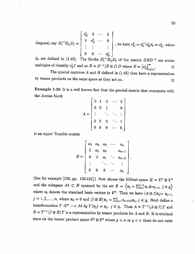
55
diagonal, say D1'B1D =
e1 '.1 0 0
0 ej 0 we have A = d'edk = e, where
0 0 ••. e
dk are defined in (1.43). The blocks DT'BD1 of the matrix DBD' are scalar
multiples of identity eI and so B = D 1 (E 01) D where E = [et]. The special matrices A and B defined in (1.45) then have a representation
by tensor products on the same space as they act on. 0
Example 1.28 It is a well known fact that the general matrix that commutes with
the Jordan block
A
is an upper Toeplitz matrix
010 0
001 0
000 1
000 ...0
a1 a2 a3
0 a1 a2 an..1
.8= 0 0 a1
0 0 0 •.. a1
(See for example [129, pp. 130-131].) Now choose the Hubert space H = C'2 0 Cn
and the subspace M C H spanned by the set B = {x1 = ej ® c5...1, j E 111
where ej denote the standard basis vectors in C,2. Then we have (A 0 I)x,= x 1,
j = l,2,...,n, where x0 = 0 and (I(9B)x5 = EL1as_i+ixs, j € z. Next define a
transformation T :C'2 — p M by T(e5) = x1, jE a. Then A = T' (A (9 1) T and
B = T' (1 B) T is a representation by tensor products for A and B. It is minimal
since on the tensor product space C" 0 C" where p < n or q < n there do not exist

56
two matrices C and D such that both C 01 and 10 D have a Jordan chain of length
n. 0
Proposition 1.27 states that the matrices A and B of Example 1.26 are a
special case of matrices that already have a representation by tensor products in the
space they act. The consequence of Example 1.28 is that in general we can not expect
the minimal dimension of a representation by tensor products to be of dimension less
than (dim K)2.
1.7 Comments
Commutative matrices have been studied since the second half of the last
century. Some of the related results were discussed in the works of Frobenius [79,
80, 81], Sylvester [158], Taber [159, 160], Plemelj [140] and Schur [148]. For a more
detailed discussion of the early developments compare [128, pp. 93-94]. It follows
from results of Voss [169] (see the remark about Schur's lectures in [146]) that an n-
tuple of commuting matrices can be simultaneously reduced to upper-triangular form.
Rutherford [146] described further properties that can be attained by this upper-
triangular form. Also Trump [164] and Egan and Ingram [62] discussed simultaneous
reduction of pairwise commuting matrices. The reduced form (1.2) that we use in
our presentation often appears in works on algebras of commuting matrices. See, for
example, the monograph of Suprunenko and Tyshkevich [154]. The authors in [154,
p.66] also noticed that commutativity of matrices is equivalent to certain symmetries
in the products of these matrices. We explore this property in greater detail. It was
shown by Gel'fand and Ponomarev [87] that the problem of a canonical form for an n-
tuple of commuting matrices contains as a subproblem the description of a canonical
form for a (not necessarily commuting) m-tuple of matrices. By a canonical form for
n-tuples of (commuting) matrices we mean a collection of n-tuples of (commuting)
matrices such that every n-tuple of (commuting) matrices would be simultaneously
similar to exactly one n-tuple in the collection. Gel'fand and Ponomarev gave a

57
canonical form for a class of pairs of commuting matrices in [86]. Though it would be
more elegant to have a canonical form for an n-tuple of commuting matrices at hand
it turns out that the reduced form (1.2) serves well for our purposes. We refer the
interested reader to [15, 77, 78, 88, 96, 121, 170] for other more recent discussions on
commuting matrices and on canonical forms for matrices.
Our motivation for studying commutative matrices comes from Multiparam
eter Spectral Theory where a special n-tuple of commuting matrices is associated with
a multipararneter system. The results of this chapter were developed simultaneously
with the results on the structure of root vectors for the associated n-tuple of commut-
ing matrices. Some of the results here were suggested by the structure of root vectors
although they are independent from Multiparameter Spectral Theory and conversely,
now form a very important building block in the theory of root vectors developed
later in this dissertation.
Our discussion of nonderogatory eigenvalues gives a different view of the
previously known results (cf. [92, p.296] or [129, p.130]). Corollary 1.7 seems to be
an interesting new observation.
The matrices RM and Ti that appear in Theorem 1.18 can be described
as solutions of linear equations in terms of the underlying multiparameter system.
Commutativity implies further symmetries on the products of matrices Ti. We as-
sociate with these products higher order tensors which are then symmetric as shown
in Lemma 1.23. These symmetric tensors appear as a coefficients in the expansion of
root vectors and their symmetry enables us to prove our main result on root vectors
for simple eigenvalues.
We remark that the results of the second section and subsection 1.5.1 to-
gether with the necessary auxiliary results are presented in [118]. We also remark
that it appears to be possible to reconstruct an arbitrary array in the form (1.2) (not
necessarily simple) from a matrix RM and matrices T7 (which are now not neces-
sarily symmetric) where m = 1, 2,. . . , M and f Ed,,,. These matrices have to satisfy
regularity and matching conditions similar to those in Theorem 1.18. Because the

58
proof of the results in this case appears to be a lengthy exercise in simple calcula-
tions and because it seems highly technically involved to apply the eventual results
to the theory of root vectors for the associated n-tuple of commuting matrices we
do not proceed with this further discussion. Let us mention however that a possible
canonical form for the matrices T7 or a canonical form for the symmetric tensors S7
could give a canonical form for the n-tuple of commuting matrices. (See [172] for a
canonical form for a special case of symmetric tensors.) The investigation of these
relations is beyond the scope of this dissertation.
In Section 1.6 we investigate the relation between an arbitrary and an asso-
ciated n-tuple of commuting matrices. Davis in [57] was first to consider the repre-
sentation of an n-tuple of commuting matrices by tensor products, which is a special
case of a representation by a multiparameter system that we define and discuss in
the next chapter. Also Fong and Sourour [75] studied the representation by tensor
products on an arbitrary Hubert space and De Boor and Rice [37] considered a re-
lated problem. As will be shown later not every n-tuple of commuting matrices is
an associated n-tuple of commuting matrices. It follows from the result of Davis [57,
Theorem 1] that every n-tuple of commuting matrices is a restriction of an associ-
ated n-tuple of commuting matrices. The problem of the minimal representation by
tensor products was stated by Davis in [57] and we will state later an analogue for
minimal representation by a multiparameter system. These problems have not yet
been solved.

59
Chapter 2
Multiparameter Systems
2.1 Introduction
We begin our discussion in this chapter by introducing the finite-dimensional
abstract setting for Multiparameter Spectral Theory in Sections 2.2 and 2.3. We fol-
low Atkinson [10, Chapter 6] who laid the fundamental tensor space construction.
Partly we also follow Isaev [112, Lecture 1]. A set of determinantal operators on the
tensor product space is induced by a multiparameter system. We assume that a mul-
tiparameter system is nonsingular, i.e., one of the induced determinantal operators,
called AO, is invertible. Then we associate an n-tuple of linear operators with a mul-
tiparameter system called an associated system. The basic property of the associated
system is that it is an commutative n-tuple. We also have the basic relation (2.7)
that connects a multiparameter system with its associated system.
At the end of Section 2.3 we include a discussion on some basic relations
between a general n-tuple of commuting matrices' and the associated system of a
multiparameter system. This is closely connected with the presentation in Section
1.6. Also Example 2.13 in Section 2.4 is related to this discussion.
In Section 2.4 we define the notions of spectra, eigenvectors and root vectors
for multiparameter system. They are defined so that they correspond to the equivalent
notions for the associated system.

60
In Section 2.5 we study root subspaces for multiparameter systems. Here we
describe a basis for the second root subspace. In the first subsection we focus on simple
and nonderogatory eigenvalues and in the second subsection we study the general
case. Relation (2.7) relating a multiparameter system with its associated system,
and commutativity of the associated system, play crucial roles in this development.
Relation (2.7) leads us to equalities of the type (2.13) and (2.23). In this way we find
vectors x that are used to construct a basis for the second root subspace. Technically
the most difficult part is to prove that the vectors we construct are actually root
vectors. We perform a direct calculation using properties of determinantal operators
and relations that hold for the vectors x. To prove completeness, i.e., the fact that
a particular collection of root vectors is a basis, we use the theory of commuting
matrices, developed in the first chapter, applied to the associated system. Certain
columns in an array in the form (1.2) are linearly independent. It turns out that they
are elements of the kernel of a special matrix that we associate with an eigenvalue of a
multiparameter system, that is the matrix B0 in the simple case (or DOA in the general
case). Because we are able to associate with a basis for the kernel of B0 (or D) a set
of linearly independent vectors in the second root subspace it follows therefore that
this set is a basis for the latter.
2.2 Notation
Assume that H1 (i E ) are finite dimensional Hubert spaces, the dimensions of H1 are ni and that Vj E £ (H1) for j = 0, 1 ... , n. Then a system of operators
is called a multiparameter system and is denoted by W. Here A = (A1, A2,... , A) E
C. We write U1 (A) = E 1 AT' j. A multiparameter system is called diagonal if
Vj = 0 for 1 ≤ i, j ≤ n, i 54 j and it is called upper-triangular if Vj = 0 for
1 ≤ j < i ≤ n. As before (cf. page 8) the transformation V € £ (H1) induces
i E n

61
Vt E £ (H) where H = H1 0 H2 0... 0 H. Note that dim = 117 n. We write
dimH = N.
The determinantal operator Ao E £(H) is defined by
L0=
itt "11
itt "21
itt "12
itt "22
'1 '2 nfl
(2.1)
The operator AO is well defined since the operators from different rows in above
determinant commute. It can be also written
AO = E (_1)3n()V1q(1) 0 V202 0•• 0 Vncy(n) EH
where sgn (ci) is the signature of a permutation ci.
Given a decomposable tensor x = X1 0 x2 0... 0 Xn E H we use the notation
i0x = E 0 V22 x2 0••• 0 Vn,()x = o.€nn
V11x1 V12x1 ... Vix1
V21x2 V22x2 ... V2flX2
vnixfl Vn2xn •.. Vnnxn
0
(2.2)
If y = Yi 0 Y2 0•• 0 yn e H is another decomposable tensor then it follows that
(i ox,y) =
yV11x1
*V VTJ 21X2
yV12x1
Y2 '222
yVnixn yVn2xn ... yVx
(The scalar product (.,•) is defined on page 8.)

62
We define further operators /j for i E 21 by
V1t1 ... Vt. 11
41 ... V2i
V t. ito Vii+i
v2t0 v21+1 (2.3)
v0 v +1 •.. vj Definition. A multiparameter system W is called nonsingular if the associated
operator A0 is invertible in £(H).
In this dissertation we study nonsingular multiparameter systems. Let us
remark at this point that the assumption 'L o is invertible in £(H)' could be replaced
by the weaker assumption that 'there exist n + 1 complex numbers Tj such that
the operator TA is invertible'. Note that the latter case can be converted
to the former by a suitable substitution of parameters A = (A0) A1, ... , A,)
homogeneous formulation of the multiparameter system
n
W(A) = LA1 Vii , i E n,
in the
j=0
i.e. substitution A = TA' where T is an (n + 1) x (n + 1) invertible matrix. So our
theory can be applied also in the latter case with minor notational changes.
Definition. The set of operators ri = L 1/ EC(H), i E z, is called the associated system (of a multiparameter system W), and is denoted by F.
2.3 Determinantal Operators
Determinantal operators retain the properties of scalar determinants when
we perform column operations.
Lemma 2.1 (i) If two columns of a determinantal operator (2.1) are interchanged,
the operator is multiplied by —1.
(ii) If two columns of (2.1) are identical, the operator equals 0.
(iii) The value of a deterininantal operator is unchanged if a scalar multiple
of one column is added to another column.

63
The proof uses the same method as in the scalar case. As a consequence
of Lemma 2.1 it follows that properties (i)—(iii) hold also for the tensor determinant
(2.2). Further we have (Laplace) expansion identities as in the scalar case. We will
use only the column versions. We write Ljk (i = 0, 1,.. . , n; j, k E i) for the cofactor of 1' in L. ik
Lemma 2.2 (i) For i, k E n we have
OjkV=ET'LOjk= o, ifi=k j=1 j=i 1 0, if ik
and
'Ojk = = k. j=1
(ii) For i,k,l En
and when k = 0
.7t ij1Vjtk T/tjL 5i=
o, if k=l=i
, if ki,k=l
— Al, if 154
0, if Ic j4l,k 54 i
= = ' 1 j=1 :1=1 1. 0, if il
The method used to prove this result is the same as in scalar case. In par-
ticular we use assertion (ii) of Lemma 2.1. Before we proceed with further properties
of the multiparameter system we need the following definition:
Definition. The decomposability set R(W) of a multiparameter system W is defined
as the set of all vectors x E H for which there exist vectors x1, x2,. . . ,x, E H such
that n
yvxj = Vio x j=1
for i€n. (2.4)

64
Lemma 2.3 Choose x € R(W) and xj, x2,. .. , x, such that relations (2.4) hold. Put
xo = —x. Then we have the identities
for i,j=O,i,....,n. (2.5)
Furthermore we have xi = r1x and so E 1 = T'x for i = 1,2,. .. , n and
= (2.6)
for i,j=1,2,...,n.
Proof. By the definition of the decomposability set the vectors x0, x1,. . . , Xn
satisfy the relations
VkX1= 0 for k=1,2,...,n.
Now we apply the operator Ljkj on the left-hand side and sum over k to obtain
EE z ikIVkx1 = o for i,j=0,1,...,n. k=1 1=0
Next the identities of Lemma 2.2 imply
o = E = —1jx5 + Aix. 1=0
Since zo is invertible we get from the above relations for j = 0 that xi =
r1x and EL1 = x. It also follows that L 1Lx = Ix = =
jL 1/.x. The proof is complete. 0
The array
v1t1 v1t ... v1Y V2f'V2t2 ... V2tn
vjlvnt2 ... Vt fin
defines a linear transformation V : H'2 —+ H". Here we write H" for a direct sum of
n copies of space H. Suppose for the moment that transformation V is not invertible.
Then the following result describes the relation between the kernels of zo and V. We
will consider this relation more closely for the special case n = 2 in Chapter 3.

65
Lemma 2.4 Suppose that x = (xi,x2,. . . ,x,,) EkerD. Then Xk € kerz 0 for all k.
Proof. We have E 1 Ox = 0 for i e . From Lemma 2.2, (i) it follows
that
o = LO1kVXj = OXk i=1 j=1
and the result follows. 0
Before we state the main result of this section we make an observation that
follows from the definition of the decomposability set.
Lemma 2.5 A vector x E H is an element of R(W) if and only if
(Vjtx, V2tx,... 7 'OX) €
Theorem 2.6 Let H, i = 1,2,. . . , n, be finite dimensional vector spaces and let W
be a nonsingular multiparameter system. Then R(W) = H, the associated operators
r1, i = 1, 2,.. . , n commute and they satisfy the relations
Er= to v j=1
for iEn. (2.7)
Proof. We only need to show that 7Z(W) = H. The other assertions then
follow from Lemma 2.3.
The adjugate operator of V is defined as
011 'O12 AOIn -
O21 'O22 A02n
On1 AOn2 Onn -
The equalities of Lemma 2.2 imply that
D.I3D=BD.V
L0 0 ... 0 -
0 zo ... 0 (2.8)

66
and hence the operator V is invertible. Then the equality H'2 = R(D) holds and thus
it follows from Lemma 2.5 that R(W) = H. The proof is complete. o
The following results are closely related to the discussion in Section 1.6. We
describe elementary relations between a general n-tuple of commuting matrices A
and the associated system r of a multiparameter system. Further research on these
relations might give an interesting new view point on commuting matrices.
The following Corollary tells us that the n-tuple of commuting matrices that
satisfies the relations (2.7) is uniquely defined.
Corollary 2.7 If A1, A2,. . . , A,, is an n-tuple of commuting linear transformations
on a finite-dimensional vector space H and W is a nonsingular multiparameter system
such that n
5=1
then A5 = F5 for j E a, where r is associated with W.
for i E 11 (2.9)
Proof. For any vector x E H the relations (2.7) and (2.9) imply
Since W is a nonsingular multiparameter system it follows from (2.8) that the oper-
ator V is invertible. Hence we have A3x = F5x for j E n and the result is proved. 0
As a corollary of Theorem 1.25 we have the following result concerning an
n-tuple of commuting operators on an arbitrary finite-dimensional vector space.
Corollary 2.8 Every n-tuple A of commuting linear transformations on a finite di-
mensional vector space K is similar to a restriction of the associated system of a
multiparameter system.
Proof. By Theorem 1.25 there exists a representation by tensor products for
A. Using the notation of the proof of Theorem 1.25 we write
Ai = T'B7T or BtI = TA1T' for iEn. (2.10)

67
If we define the multiparameter system W by W1 (A) = IA, - B1, i = 1,2,.. . , n, then
it follows that F, = BI. Therefore it follows from the relations (2.10) that A is similar
to a restriction of the associated system r. 0
Corollary 2.9 Let A1, A2,... , A, be an n-tuple of linear transformations on a finite-
dimensional vector space K. Then the following are equivalent:
(i) the transformations A, commute
(ii) there exist a multiparameter system W, a common invariant subspace M for
associated transformations F1 and an invertible linear transformation T K -
M such that n
T'TA5 = VT for to 2=1
Proof. It follows from the previous corollary that assertion (i) implies asser-
tion (ii).
Now assume that (ii) holds. As in the proof of Corollary 2.7 it follows
that TA5T'x = T5x for all j and all x E M. So A5 are simultaneously similar to restrictions rj Im and therefore they commute. 0
We say that an n-tuple A of commuting matrices on Hubert space K has a
representation by a multiparameter system if there exist a multiparameter system W
with associated system r acting on a Hubert space H, a subspace M C H invariant
for all F1 and an one-to-one map T: K —+ M such that
T'F1T = A1 for i E i.
Theorem 1.25 tells us that every n-tuple of commuting matrices has a representation
by tensor products which is actually a representation by a (special) diagonal multi-
parameter system. The natural question arises what is the minimal dimension of
the space H on which A has a representation by a multiparameter system ? This
is still an open problem. Example 2.13 below shows that A does not always have a
representation by a multiparameter system on the original space K. First we need to
establish some more properties of multiparameter systems.

68
2.4 Eigenvalues, Eigenvectors and Root Vectors
of a Multiparameter System
Definition. An n-tuple A = (A,, A2,. . . , A,) E C" is an eigenvalue of a multipa-
rameter system W if all the operators —V + E., AV2j, i E n are singular. The
collection of all the eigenvalues of the system 1W is the spectrum of W and is denoted
by 0(W).
The following proposition is a standard fact. We state it because we later re-
fer to it. It can be proved in the finite-dimensional case using a dimensional argument
(cf. Atkinson [10, pp. 72-73]).
Proposition 2.10 Suppose that V E £(H), i € n, and H = H, 0 H ®... ® H,,.
Then it follows that
flkerT/t =®kerV
Atkinson [10] proved the next important result connecting the spectrum
of a multiparameter system W and the spectrum of its associated system. It also
describes the eigenspace of the associated system r. We include, for the completeness of presentation, the proof following Isaev [112].
Theorem 2.11 The spectra of a multiparameter system W and its associated sys-
tem r coincide. If A E o(W) then the space of common eigenvectors for r at the
eigenvalue A is n n
flker (AI—r) =ØkerW(A). (2.11) i=1 i=1
Proof. Assume that A€a(W) and that yi € ker W\ {0}, i E R. Write X = Yi ®Y2O...O n and xj = Aix. Then = 0 for all
and hence x E R.(W). Lemma 2.3 then implies that rjx = xj = Aix. So we have
A E o(F) and ØL1 ker W1(A) C fl., ker (AI - ri).

69
Now assume that A E cr(r) and that a vector x E fl 1 ker (A11 - r1) \ {o}. Then relations (2.7) yield
0 VAx — Vx = T4T.(A)tx
Proposition 2.10 implies that fl 1 ker W1(A)t = Ø ker W1 (A) and therefore it fol-
lows that x E Øt=1 ker W1(A) and A E o(W). 0
Next we choose, for every i, a subspace Hil C H1 such that H, = ker W1 (A) e H,'. For later reference we also need the next lemma.
Lemma 2.12 Suppose that a vector x1 E (ker W1 (A)*)±. Then there exists a vector
Yj E H such that x1 = W1 (A) y.
Proof. Suppose that x1 E (ker W (A)*). Because
(kerWj(A)*)i = fl.(W1(A))
it follows that there exists a vector z1 € H1 such that x1 = W1 (A) z1. By the definition
of the direct sum of vector spaces we can find vectors Yl E H and wi E ker W1 (A)
such that y + wi = z1. Then it follows that x1 = W1 (A) y. El
We now state the example, promised on page 67, of commuting matrices
that do not have a representation by a multiparameter system on the original space.
Example 2.13 Assume that
A=
0000
0000
0001
_0 0 0 0_
and B=
0 0 a1
0 0 0 a2
0 0 0 a3
0000
and that a1 154 0. It is easy to see that AB = BA = 0. We w ill show that A I a2 I
and B do not form an associated system of a (nonsingular) multiparameter system.

70
Assume the contrary. Since A and B have a three-dimensional subspace of common
eigenvectors they could arise from a multiparameter system W only with n1 = 1 and
n2 = 4 (see Theorem 2.11). Write MT as
W1 (A) = v1)1 + v2)2 - VO
W2(A)=V1A1+V2A2_V0
Then we have
F1 = (viV2 - v2Vi)' (voV2 - v2Vo) and r2 = (viV2 - v2Vi)' (viVo - voVi).
The equation (2.7) for i = 1 is v1F1 + v2F2 = v01. If F1 = A and F2 = B then it
follows that v0 = 0, a, v2 = 0 implies v2 = 0 and also v1 + cx3v2 = 0 implies I a2
vj. = 0. This contradicts the assumption that W is nonsingular. Hence the matrices
A and B are not the associated system of a multiparameter system. 0
The main topic of our study is to describe a basis for the root subspaces
of the associated system of commuting matrices r in terms of the corresponding
multiparameter system W. The results of Chapter 1 showed that two extreme cases
of commuting matrices that are easily understood are the case when the coinmuting
matrices are represented by tensor products (i.e., A acts on a space H1 0 H2 ®
(D H, and A1 = B7 where B1 E £ (H1)) and the nonderogatory case. The first
case corresponds to a diagonal multiparameter system with identity matrices on the
diagonal (see Example 2.14) and is easy to deal with. The nonderogatory case is yet
to be defined, but for the moment we call an eigenvalue A E c (W) nonderogatory
if it is a nonderogatory eigenvalue for a commutative n-tuple F. Later we will be
able to define a nonderogatory eigenvalue completely in terms of the multiparameter
system W.
Example 2.14 Assume that a multiparameter system is diagonal with Vii = I, for
all i. Then we have F1 = V. Choose an eigenvalue A e o (W) and suppose that

71
{ X ; ki E pj, 1 E qki is a complete system of Jordan chains for Vo at A,. Proposi-
tion 2.10 implies
fl ker (A11 - = fl ker ((A11 -' = Øker (A11 -
and therefore
{x1,lk1 øX2k21k2 0••• 0 xflkfl Ik ; 1ki E q, k1 E pi, i E Al
is a basis for fl .1 ker (Ail - T1 )N . Write k = (k1, k2,. .. , k,) and I = (li, 12,... , la).
The action of A,I - ri 011 k1 = X1k1 11 ® X2k2 12 0 0 Xnkn 1n is (AI - F1) zkl =
4 where 1' =(l,... , lj, i - 1, l.i,... , li,) and zk1 = 0 if 1i = 1. Each F1 has
q Jordan chains of lengths qk1 , k1 E pi at eigenvalue A. 0
Before we state the next definition we recall that the subspace ker (Al -
for a set of commuting linear transformation r was defined on page 10.
Definition. Suppose that A E o• (W). Then we call the subspace ker (M\I -
the root subspace (of W at A). We call the subspace ker (Al - r)m for m = 2,3,... the m-th root subspace (for the multiparameter system W at the eigenvalue A) and
for m = 1 the eigenspace of W at A.
A nonzero element of ker (Al - r)r is called a root vector. Also a nonzero element of the m-th root subspace is called an m- th root vector if m ≥ 1 and a nonzero
element of the eigenspace is called an eigenvector.
Note that a lc-th root vector is also an l-th root vector if k < 1.
2.5 A Basis for the Second Root Subspace
Our main objective in this dissertation is to describe a basis for the root
subspace using the multiparameter system SAT directly, i.e., without using the tensor
product constructions Lj etc. This is particularly important in infinite dimensions,
but also for matrices it offers an advantage on dimensional grounds. In this section
we describe a basis for the second root subspace.

72
2.5.1 Simple Case
First we consider the space ker (Al - )2 for eigenvalues that have one-
dimensional eigenspaces, i.e., when d0 = dim ker (Al - = 1. By Theorem 2.11 we
have d0 = 1 if and only if
dim ker W 1 (A) = 1 (2.12)
for all i. Then we choose x0 E ker W1 (A) \ {O} and yo E ker W1 (A)* \ {O}, so W1(A)x10 = 0 and yW1(A) = 0. The vectors zo = x10 0 x20 0 ... 0 x 0 and
Wo = Yo 0 0 0 are, respectively, right and left eigenvectors for all
The following proposition gives some necessary and sufficient conditions for a root
vector of r, i.e. a vector z1 E H\ f 0 such that (.\I - r1) z1 = a1z0 for each i and not all a1 E C are zero, to exist. As before (see page 69) we denote by H a direct
complement of the kernel of W1 (A) in H1.
Proposition 2.15 The following statements are equivalent:
(i) There are a E C'3\ {0} and x11 E H such that
= W (A).Til
for i E 22.
(ii) There is a E C'\ f 0 such that
for i E n.
(iii) wL 0z0 = 0.
(2.13)
yUj (a) x10 = 0 (2.14)
(iv) There exists an index i such that r, has a root vector at A1 corresponding to z0. (That is there exists a vector z1 E H\ f 0 such that (A11 - T1) z1 = zo.)
(v) ker(AI — F) 0 ker (AI —F)2.

73
(vi) There are a E C\ {O} and Yii E H1 such that yU1(a) = y1Wj (A) for i E n.
Proof. It is easy to observe that (i) implies (ii) and (vi) implies (ii).
Assume (ii). Then it follows U1 (a) x10 E (ker (W1 (A) *)) -' and then by Lemma 2.12 there exists a vector x11 e H' such that U1 (a) x10 = W1 (A) x11. This
proves (i), and similarly (ii) implies (vi). So (i), (ii) and (vi) are equivalent.
The system of equations (2.14) has a nontrivial solution a if and only if the
determinant of the system
Yb* liXbO
y0V21x20
y0V12x10
y0V22x2g
* Yb vTi lnXbO
Yov2nx2o
Yn*O flflXfloj
= W/0Z0
equals 0. Thus (ii) and (iii) are equivalent.
Suppose now that (i) holds. Write
=X10 ® 0 Xil 0 ... 0 x. (2.15)
Using the properties established in Lemma 2.1 and assumption (i) we can make the
following calculation:
(A1zo - z1) z1 =
vifi ... Vii,_i W 1 (X) v1 ... v1t7 V2i,_i W2 (A) t V21+1 ... Vt
n.j—i W (A) i'ç j+1
V11x10 ... 0
• vj_i,i_ixj_i,o 0
Vj,i_ixji (J (a) x0 V,11x1
0
vn,i_ixno 0 V,1+1x0
vnfn
zi =
V1nX1O
Vi—i,nxj—i,o vjnxji
T/+i,nxj+i,o
vnnxno
0
(2.16)

74
The value of the determinants above remains the same if we replace the terms
k = 1,. .. , i - 1, i + i,... , n, by Vjkxjo. Then by Lemma 2.1 the sum (2.16) equals
V11x10
V21x20 V2,-1x20
U1 (a) x10
U2 (a) x20
Vi,1+ixio Vi,x10
v2,i+1x20 v2nx20
vnoxno ... Vn.i_ixno U, (a) XnO V1x0 ... vnnxno
0
= aL.0z0,
where a = [a1, a2,... , an IT Therefore z1 E ker (.XI - F)2 / ker (U - F), i.e., (v) holds.
It is trivial that (v) implies (iv), so assume now that (iv) holds, that is
(Az0 - z) z1 = L0z0.
We also have w t7jo - j) = 0 and hence property (iii) follows since
O *f\ —wo vi 0_ Ai) Zi=W0* 0Z0.
The proof is complete because we have established the implications (i) =
(v) (iv) = (iii) and the equivalence between (i), (ii), (iii) and (vi). 0
Remark. Suppose that the conditions of Proposition 2.15 hold. Because a 54 0 there
is at least one index h such that ah 54 0. Then (XhI - r'h) z1 0 0 and (AhI - rh) ZO = 0
and therefore the vectors z1 from (2.15) and z0 are linearly independent. This cannot
be established when Ao is singular as shown in the following example. Therefore
the assumption that the multiparameter system W is nonsingular is essential for our
discussion. 0
In the next example we identify the tensor product x1 0 X2 of two vectors
x11x21
FS11 1 2 F 21 1 2 11 22 = I I E C and 2 = I E C with the vector , and similarly [ 12 ] I 22 J 1221
1222
we identify the tensor product V11 0 V22 of two matrices Vii, V22 E C 2x2 =
[V11 V12 J with the matrix I 11V22 v12V22 1 V
V21 V22 [ v1V22 v22V22 j Later we use this construction,

75
that is sometimes called the Kronecker product of two vectors and two matrices,
respectively, also for the tensor product of two vectors from arbitrary vector spaces
C' and cm and for two arbitrary, k x 1 and m x n, matrices.
Example 2.16 Suppose that
1 W, (A) IA1+I [1 0] _i _1] 0 —1
and
W2(A)= I I Ii ol A, I —1 ii x2 1 —11 —1 1 0] [_1 OJ [0 —2
Then Then
101
0000
—1 1 1 0
—1 0 1 0
is a singular matrix and so W is a singular multiparameter system. Suppose that
A0 = (1, 1). Then
Wl(Ao)=[1 i] and W2(Ao)_[0 2] and thus A0 € o (W). We choose
111 F 1 1 Iii 11 Xçj = I I Yio = I I , x20 = and 1120 =
LoJ 1-1 I .
The pair of equations (2.14) for a = ai 1 reduces to a single equation a1 - a2 = 0. L a2 J
We choose a = The vectors x11 = and X21 = 0 [] are such that U (a) xo = W (A) x1 for i = 1, 2, and then the vectors z0 =
are linearly dependent, but - z1) z1 (Lo - L2) z1 =
1
0
1
0
0
and z1 =
0
0
0
0 0

76
Suppose that A E o (IV) is such that the relations (2.12) hold. We restrict
our attention to the root subspace A/ = ker (Al - F)N and we bring the restricted
transformations (\I - r2) -, that are commuting and nilpotent, to the form (1.2),
i.e.,
0 A°' A°2 ... AOM -
0 0 A'2 ... Aim
(AT - F) LV=
o 0 0 •. A m-1,m
00 0... 0
where the array Aki has sizes dk x d1 x n, and, by definition,
= dim ker (Al - F)'' - dim ker (Al - p) /C (2.17)
for k ≥ 1 and d0 = dim ker (Al - r). Because we assumed (2.12) holds for A it follows
that d0 = 1. We use the notation (1.3) for the arrays Ak1 and the notation (1.4) for
the n-tuples aii .
Next we write
B0=
* Yb* llX lO Yi*o 12XlO .. YlO lnxbo
y0V21x20 y0V22x20 ... y0v2nx2o
yoVn1xno y:ov2i;o ...
(2.18)
This n x n matrix will play an important role in the following proposition. We recall
that the subspace H C Hi is a direct complement of the kernel of W (A). It was
introduced on page 69.
Proposition 2.17 Suppose that A E o (W) and that dim ker W (A) = 1 for i =
1, 2,. . . , n. Then d, = dim ker B0 and the set {a'; k E d,} is a basis for ker Bo.
Furthermore there exist vectors x, E H such that
(a) U (ag') xio = W (A) 4,

77
(b) the vectors 4 = E 1 x10 0... 0 x_1,o 0 x 0 x.j,0 0 0 x,, k E d1 together
with the vector z0 form a basis for ker (Al - F)2, and
(c) (A21 - r) 4 = aJzo.
Proof. Write dim ker B0 = d and assume that a1, a2,... , ad E Cn form a
basis for ker B0. So we have
yjT/akJxo =O, for iEfl and kEd. j=1
Because the statements (i) and (ii) of Proposition 2.15 are equivalent we can find
vectors x e H such that
W (A) Xk ii = U (ak) XiO (2.19)
for all i and k.
The same calculation as in the proof of Proposition 2.15 which showed that
(i) implies (v) proves that
(AI - r) 4 = aklzo, for i E a and k E d.
Here 4 = E1 x10 a... ® Xj1,0 0 Xj 0 Xj14,0 ®... X,.
Let 180z0 + EL /3k4 = 0. Then 0 = - r) (10z0 + ,84) =
E=1 akI3kz0 implies /3k = 0 for k E , and then /30z0 = 0 implies PO = 0. So
{ zo, z11,... , z} are linearly independent, whence d < d1 and we can assume that a1 = ak for k E d.
To complete the proof it suffices to prove the opposite inequality, i.e., d ≥ d1.
We choose vectors z11, 4,... , z so that they form together with the vector z0 a basis for ker (Al - F)2. By Proposition 1.2 it follows that n-tuples
Z101 = { a a2 ... a T
k E d1 are linearly independent. We also have
(I - r) 4 = for i E z and k E d1. (2.20)

78
The relation (2.7) proved in Theorem 2.6 implies that
n
Or =
j= 1
for all i and k. It follows then from (2.20) that
W1 (A) z1k - U - (2.21)
Now we choose for every i an element u E H1 such that ux10 = 1. This is possible
because x10 0 0. If we multiply the relation (2.21) by
on the left-hand side it follows that yU1 (a2') x10 = 0 for all i and k. This proves that
the n-tuples a?', a1,. . . , a E ker B0. Since they are linearly independent it follows
that d ≥ d, as required. 0
An immediate consequence of Proposition 2.17 is the next corollary.
Corollary 2.18 An eigenvalue A E 0 (W) is nonderogatory if and only if
and
dim ker W1(A)1 for iEn
rank Bo≥n-1.
Proof. Theorem 2.11 implies that d0 = 1 if and only if dimkerWj (A) = 1
for all i and Proposition 2.17 implies that d, 1 if and only if rank B0 ≥ n — i. From
Corollary 1.7 it follows that an n-tuple A is a nonderogatory eigenvalue for r if and only if d0 = 1 and d1 1. Hence the result is established. C1
Using the result of Corollary 2.18 we are able to make the following defini-
tions
Definition. An n-tuple A E C is called a nonderogatory eigenvalue for a m'altipa-
rameter system W if dim ker W1 (A) = 1 for all i and
rank B0 ≥ n — 1. (2.22)

79
The matrix B0 is defined in (2.18).
Definition. An n.-tuple A E C is called a simple eigenvalue for a multiparameter
system W if dim ker W1 (A) = 1 for all i and
rank B0 ≤n-2.
Note that an eigenvalue A is simple eigenvalue* for a multiparameter system
W if and only if it is a simple eigenvalue for the associated system F.
2.5.2 General Case
In this subsection we omit the assumption (2.12), i.e., the dimensions qj =
dim ker W1 (A) are now arbitrary. First we need an auxiliary result.
Lemma 2.19 Let the vectors xiji E H1, ji E qj, i = 1,2,... ,k - 1,k + I,— , n' be
linearly independent and suppose that
Z = x111 (8) ... 0 Xk_1,jk_l 0 jl ® Xk+1,jk+l (8) ... 0 xnj = 0
where xk € 11k and the summation runs over all multiindjces j' = (ji, . .. ,
.Jk+1 ... ,3n),iiEqi,i=1,2,...,k_1,k+1,..,n Then xJ'.._o for all jF
Proof. Suppose that Xkjk, .1k E nk is a basis for Hk. Write q,, = nk and
= E 1 &Xkjk for every j', where j = (jl,j2,. . ,3k-1,jk,jk+1,. . . , in) . Then
= C•Xljl 0• ® Xk_1,jkl ® X kjk0 Xk+1,jk+l (D ... 0 j
where summation runs over all multiindices j E q x q2 x ... x q,2, and since vectors
0 x22 0 xnjn, ii E qj, i E n are linearly independent it follows that Qi = 0 for all j. Thus it also follows that xj,' = 0 for all Y. 0
Let us introduce some notation. Assume that the vectors x E H1, k E q1
form a basis for the kernel ker W (A), i E A. We define the set of integer n-tuples
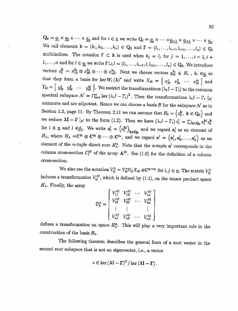
80
Qo = qi x q2 x ... X q and for i e n we write Qt = q1 x xq1_1 x qj x x q,.
We call elements k = (k1, k2,. .. , k,) E Qo and 1' = (ii, . . . , ,in ) E Q
multiindices. The notation 1' C k is used when k1 = ij for j = 1,. . . , i - 1, i +
1,..., n and for i E qj we write 1' Ui = (ii,. . . . . . ,l) E Qo. We introduce
vectors z = ® x ® 0 x. Next we choose vectors y3 E H1 , k1 Eqj so
that they form a basis for ker W1 (A)* and write X10 = { x 4 ... Xiqi o J and Yio = [Yio y •.. y7 J. We restrict the transformations (A11 - F1) to the common spectral subspace Al = flL, ker (A11 - r)2. Then the transformations AI - ri I.v commute and are nilpotent. Hence we can choose a basis B for the subspace Al as in
Section 1.2, page 11. By Theorem 2.11 we can assume that Bo = {z, k E Qo} and
we reduce Al - F Jr to the form (1.2). Then we have (A21 - 1) z = kEQ0 a1z
for i E and 1 Ed,. We write a = (a 1)kQ and we regard all as an element of
HA, where H), =C" ® 0 jjq and we regard a1 = . . ,a) as an
element of the n-tuple direct sum H. Note that the n-tuple a1 corresponds to the
column cross-section C' of the array A°'. See (1.6) for the definition of a column
cross-section.
We also use the notation = Yio V2jX10 E' for i,j E 22. The matrix 13
induces a transformation T'13 , which is defined by (1.1), on the tensor product space
H),. Finally, the array
Do'=
V1t V,.t ... V1 n
V2t V2 't ... V2 nt
TI n1 "M TI n2M TIM '
defines a transformation on space H. This will play a very important role in the
construction of the basis B,.
The following theorem describes the general form of a root vector in the
second root subspace that is not an eigenvector, i.e., a vector
E ker (Al - F)2 / ker (Al -

81
Theorem 2.20 A vector z is in ker (AT - F)2 / ker (Al - F) if and only if there exist
n-tuples ak E C", not all 0, for k E Qo and vectors x E H, k' E Q, i E z. such
that
and n
qj
>2 U (ak'uu1) x = W (A) xh') k=1
(2.23)
Z =>2 >2 k. 40... ® ® x ® (9) ... ® x. (2.24) i=1 k'EQ
It then follows for all i that
(A11 - r) z = >2 (2.25) kEQ0
Proof. Suppose that z is in the form (2.24). Then the following direct
calculation shows that (2.25) holds and since not all ak are 0 it then follows that
z E ker (AT - F)2 / ker (Al - F). In the calculation we use the elementary properties
of determinantal operators from Lemma 2.1 and relations (2.23), and proceed similarly
as in the proof of Proposition 2.12, (i) implies (v)
V114 ...
n (AiLo — Ai) z=E >2
j=1 k'EQJ
v14
Qi 0 ... ± j(a1c)4 ... 0
V ix,j 0 •.. V,,,x nno
Viix U1 (ac) x v17,x
= >2 V21x U2 (a1) X'2f) V2 n XJ220 = >2 aL0z. kEQO : : k€Q
v1x U,, (ak) x Vfl,,4,J
Now assume that z E ker (AT - F)2 / ker (AT - r). Then we have (2.25) for
some aik E C, k E Qo and i = 1,2,. . . , n. We also write ak = [a a a jT E
C". The relation (2.7) then implies
W (A) z = >2 VA (Ail - r) z = >2 >2 az = >2 U (ak) t z (2.26) 3=1 i=1 kEQo k€Qo

82
for all i. After we multiply (2.26) with i') on the left-hand side it follows that
E x 0... ®ki 0 > 0 x ' ® 0 x2 =0. kEQO j=1
Since x are linearly independent it follows from Lemma 2.19 that
gin
> = 0 k1=1 j=1
for all k' E Q, and every i. Thus we have qi
u (ak'i) x E (kerW (A)*) k=1
and then, by Lemma 2.12, there exist vectors x E Hi such that relations (2.23)
hold. Here the subspace H C if1 is a complement of the kernel ker W1 (A) as defined
on page 69. Now we can construct a vector
= X 0•• 0 Xjbo 0 x 0 0... 0 x. (2.27) j=1 k'EQ3
The same calculation as above shows that (A11 - r1) z' = EkEQO Then we have
z - z' E ker (Al - F) and thus there exist complex numbers /3k, k € Qo such that
Z = z' + EkEQO /3kz. If we substitute the vectors x + E =1 I3k'uk1 x for the vectors
A11 in the expression (2.27) it follows that
1=1 k'EQ,
and, since (2.23) and (2.25) are unaffected by this substitution, the proof is complete.
0
The following theorem extends Proposition 2.17 to the general case. As
before we restrict our attention to the second root subspace .A/ = ker (Al - F)2 and we
bring the restricted transformations (A21 - r1) Jg, that are commuting and nilpotent, to the form (1.2). See also page 76 for details. We also recall that the n x (fl qi)
column cross-section of the array A°1 is regarded as an element of H. (Cf. page 80.)

83
Theorem 2.21 Suppose that a1 E H, 1 = 1,2, . . . , d1 are the columns of the array
A°'. Then they form a basis of ker D.
Conversely, to any basis {al, 1 = 1,2,. .. , d} C H of ker V we can asso-
ciate a set of vectors B' = {z, 1 = 1,2,. . . , d1} c H such that Bo U /3' is a basis for
ker (AT - F)2 and (AI - 1'1) z'l = EkEq0 a,•'zok for all i and 1.
Proof. Suppose that {Zj, 1= 1,2,... ,d2} u {z, k E Qo} is a basis for ker (AT - F)2. Then we have (A11 - 1'1) zl = EkEQO a•, 'zok and the relations (2.7)
imply
W (A) z = v (A31 - r) = > =
j=1 i=1 kEQQ
n
= E keQ0 1=1
After we multiply the above expression with 1' on the left-hand side it follows that
E x 0••• øxj ØEa'YVjjx ki (9 9) nO = 0. kEQO 1=1
Since x are linearly independent it follows by Lemma 2.19 that
= 0 k=1 j=1
for all k' E Q, and all 1. This can be written as
>Vta1 = 0. j=1
Hence it follows that a1 € ker DA for all 1. Proposition 1.2 implies that a1 are linearly
independent and so it follows that
c1 ≤ dim ker D. (2.28)
Next we will show that to every a E ker D we can associate a vector z1 E
ker (AT - F)2 \ ker (Al - F) such that
(AI - r1) zi = (2.29) kEQO

84
Because a is in the kernel of V it follows that T'a = 0 for all i. This is
equivalent to
Y . o = io Vjja'Uulx = : u (a''i ) ki
k1=lj=1 k=1
for all k' = (k1, . . . , k1_, k1+1,. . . , k,) E Qj and all i. From the above equations it
follows that U1 (akh1J1) x E (kerW1 (A)*) -L. Lemma 2.12 implies that there
exist vectors x E H such that
qi
u a k'Uiki x = TV1 (A) il x. k=1
As in the proof of Theorem 2.20 it follows that the vector
71
Zi
3=1 k'Q1
is such that relations (2.29) hold. Then, if {a1, a2,... , ad} is a basis for ker V, we
can associate with every a1 a vector z1 = as above. The vectors z, 1 = 1, 2, . . , d
are linearly independent because
(A1I—r)z= az
k€Q0
and al are linearly independent. Thus it follows d1 ≥ dim ker V and together with
(2.28) we obtain d1 = dimkerV. The, proof is complete. 0
We illustrate the theorem with an example.
Example 2.22 Consider the two-parameter system
and
W1(A)=
W2(A)=
100
010
011
100
000
001
A1+
100
0 1 1 2 2
01 1
000
A1+ 0 1 1
010
A2 -
A2 -
0 —1 0
0 1 1 2 2
000
0 0 —1
002
002

85
Evidently the matrices V10 and V20 are singular. So Ao = (0,0) E U (W) and we have
dim ker V10 = 1 and dim ker V20 = 2. Hence d0 = 2. We choose
X10 =
1
0
0
Y10 =
0
0
1
Then it follows that vectors
zOlb —
-
1
0
0
0
0
0
0
0
0
1
0
0
2_ X20 -
and z2 =
0
1
0
0
0
0
0
0
0
0
1
0
and Y20 =
22
10
01
form a basis for ker r and we have
V10=V10 __[O], V0= [ °] and4 0=[ 1• The space HH,\H,,,\,, = C 0 C2 and we identify the direct sum H.\0 ED H, with C4.
Then
01

86
1
Because the matrix V° has rank 1 it follows that d1 = 3 and we choose a1 =
a2 =
0
1
0
0
and a3 =
0
0
1
0
0
0
—2
to form a basis for ker V. To construct a vector z11
corresponding to a1 we need to find vectors x11 , x and Al21 such that
V11x10 = W1 (.Xo) x, —2V12x10 = W1 (A0) x11 and V2jx0 - 2V22x0 = W2 (A0) x.
A possible choice is
Similarly we find vectors
that correspond to a2, and vectors
0
0
0
21 -
ii -
22 -
ii -
23 -
ii -
0
—2
2
0
0
0
and x =
and x =
and x1321
0
0
1
0
0
0
0
0
0

87
that correspond to a3. Then
0
0
1
1
—2
0
—1
2
0
zi =
0
0
0
1
0
0
—1
0
0
and {z0', 4; z, 4, 4} is a basis for kerr2.
2.6 Comments
and 4 =
0
0
0
0
1
0
0
—1
0
0
Multiparameter Spectral Theory has its origins in the work of Klein [117],
Bôcher [32, 33, 34], Dixon [59] and Hilb [104, 105] late in the nineteenth century.
Also Hilbert [106] and his students considered problems in Multiparameter Spectral
Theory. When solving certain boundary value problems by the separation of variables
technique we are led to a system of differential equations that are linked only by
spectral parameters and this linkage is linear. This is the underlying motivation for
many of the developments in Multiparameter Spectral Theory. Some examples of
such boundary value problems are the classical ones of acoustic or electromagnetic
vibrations and different linearised parts of various bifurcation models involving several
parameters as in rotation, convection or explosion. The problem of oscillation of an
elliptic membrane is an example that yields two separate differential equations that
both contain two spectral variables in a nontrivial fashion, while for example the
problem of oscillations for a rectangular membrane leads to a diagonal case and for
a circular membrane leads to an upper-triangular (also called mildly coupled) case.
The last two cases can be solved using only techniques from the one-parameter case.

88
The example of the elliptic membrane and similar situations led to studies of special
functions at the beginning of this century. Erdélyi gathered such results in [64]. (See
also the book by Arscott [6].)
Carmichael [50, 51, 52] was the first to consider multiparameter eigenvalue
problems in an abstract setting. He studied, for example in [50], a finite-dimensional
multiparameter system generated by a difference equation approximating a system of
integral equations. It was Atkinson [10, 8] who laid the foundations of modern Ab-
stract Multiparameter Spectral Theory which led to a revival of the theory in the last
30 years. In the 70s Multiparameter Spectral Theory in an abstract Hilbert space
was developed by Binding, Browne, Faierman, Källström, Roach, and Sleeman, to
mention a few, in a number of contributions (see Browne's review article [42] and also
the enclosed list of references for details). Many of these were brought together in the
book by Sleeman [153]. Work on extending multiparameter eigenfunction expansion
theorems in a number of directions and under various "definiteness conditions" has
been done recently by Binding, Faierman, Gadzhiev, Isaev, Roach, Volkmer and oth-
ers. Also the recent books of Volkmer [168], Gadzhiev [84] and Faierman [69] present
several results on eigenfunction expansion. We also remark that most of research
so far involved self-adjoint multiparameter eigenvalue problems. As an exception we
mention the paper of Allakhverdiev and Dzhabarzade [2] where they considered a
normal multiparameter system, i.e., a system where all the operators Vij are normal
operators.
The fundamental tensor space construction that we introduce in this chapter
was given by Atkinson in [10, Chapter 6]. In our discussion we partly follow also the
presentation of Isaev [112, Lecture 1]. For instance, the idea to use the decomposabil-
ity set to prove commutativity of the associated system and relation (2.7), is found
in [112] (cf. also [4]) where it is used in the infinite-dimensional setting. The notions
of-spectra, eigenvectors and root vectors for multiparameter systems are defined to
correspond to the equivalent notions for the associated system. The corresponding
notion of Taylor's spectrum, introduced by Taylor in [161] for an n-tuple of commuting

89
operators, was defined for multiparameter systems by Isaev and Fainstein [111] and
studied by Rynne [147]. See also Isaev's Lecture 5 in [112]. In the finite-dimensional
setting the notion of Taylor's spectrum for a multiparameter system coincides with
the spectrum as defined in Section 2.4.
The linear transformations associated with the square arrays of operators,
for instance our transformations V and V, are an important tool in the presentation.
They were studied already by Atkinson in [10, Chapter 8]. He proved that if there is a
nonzero element in the kernel of such a transformation then there is a decomposable
element in that kernel (cf. [10, Theorem 8.5.1]). This enabled him to weaken the
regularity condition and still prove the expansion result ([10,.Theorem 10.6.1]). An
interesting related investigation is found in paper of Allakhverdiev and Dzhabarzade
[1]. They discuss relations between vectors V3x, j = 1, 2,. . . ,k, where i = 1,2, .. . , m
and k, n > 2, for which E V1x1 0 V25x2 0 0VnjX,, = 0.
The structure of the second root vectors in the simple case (cf. Subsection
2.5.1) follows the one of root vectors in Binding's paper [23]. In the general case the
transformation V carries information about the second root subspace. This will be
examined in detail for two-parameter systems in the next chapter.

90
Chapter 3
Two-parameter Systems
3.1 Introduction
In this chapter we use a matrix equation of Sylvester type to study two-
parameter systems
W1(A)=V1A1+V2X2—Vo, i=1,2. (3.1)
First we briefly describe our main ideas.
We identify the tensor product space Cq, ® jJt72 with the space of q x q2
complex matrices via the isomorphism : CO Xq2 defined by
all
aq1l
a12
aq12
alq2
aq1 q.
all a12 alq2
a21 a22 a2q2
aqil aq12 • aq1q2 -
(3.2)

91
It was shown in Section 2.5, page 80 that we can associate a transformation V' with
an eigenvalue A E ci M. In the two-parameter case we view
ç7iiAt v
-
tiM V21
tiM "12
T/M V 22
via the isomorphism , as a transformation acting on the vector space of pairs of
qi x q2 matrices. We also consider the determinantal transformation
L = ViAiØV2 _ViA2ØV2)i
as a transformation on the vector space of complex q1 x q2 matrices. There is a close
relation between the kernels of DA and of z as shown in Lemma 2.4. We restate it
here in the above setting.
Corollary 3.1 Suppose that X = X1 , xi, x2 E C q,xq2 is an element of the x2
kernel ker D. Then both X1 and X2 are in the kernel ker.
In Theorem 2.21 we showed how to associate a basis for the second root
subspace with a basis for the kernel of V, the above result relates this kernel to the
kernel of AA , and a matrix X e ker L if and only if V/jXT4 - VjXV = 0. This is
our motivation to study the matrix equation
AXDT - BXCT =0. (3.3)
To do so we use the Kronecker canonical forms for pairs of matrices (A, B) and (C, D).
We describe this special block diagonal form for a pair of matrices in the next section.
With every block in the Kronecker canonical form of a pair (A, B) we associate an
invariant and a chain of vectors called a Kronecker chain. The invariants are of three
different types. So, when we study equation (3.3) we would have to consider nine
different cases, but because of symmetry with respect to the pairs (A, B) and (C, D)
we only need to study six different cases. For any of these cases where there are
nontrivial solutions of equation (3.3) we give a basis for the subspace of solutions

92
in terms of underlying Kronecker chains in Subsection 3.2.2. Similarly we study the
space of solutions of a pair of equations
AX, + BX2 =0 and X1CT + X2DT =0 (3.4)
in Subsection 3.2.3. Corollary 3.1 is used to relate this system to equation (3.3).
With every pair of invariants of (A, B) and (C, D) for which there is a nontrivial
solution of the system (3.4) we associate another invariant. We show in Section 3.3
that when a set of invariants is associated this way to pairs of matrices (va, v) and (va, v2) it is equal to the set of invariants of the pair of matrices (Al, A2). Here a pair of commuting nilpotent matrices A2 = (A21 - r) Ik (AIr)2' i - 1, 2 is brought
to the form (1.2) and the matrices A1 and A2 form a subarray A' of the array A°' as described in Example 3.3. We also construct a basis for ker iI - F)2 such that
the pair of matrices (A?1, A') is in Kronecker canonical form and we illustrate the
construction with two examples.
3.2 Kronecker Canonical Form and a Special Ba-
sis for the Space of Solutions of the Matrix
Equation AXDT - BXCT = 0
3.2.1 Kronecker Canonical Form
We refer to [85, Chapter XII] or [92, Appendix] for recent presentations of
the Kronecker canonical form. Our presentation is based on a disposition by Professor
H.K. Farahat in a private conversation.
Definition. A pair of complex m x n matrices (A, B) is equivalent to a pair of
matrices (C, D) if there exist invertible matrices P E C'2<' and Q E Cm<m such that
C = PAQ and D = PBQ. (3.5)
First we introduce some special matrices needed in the construction of the
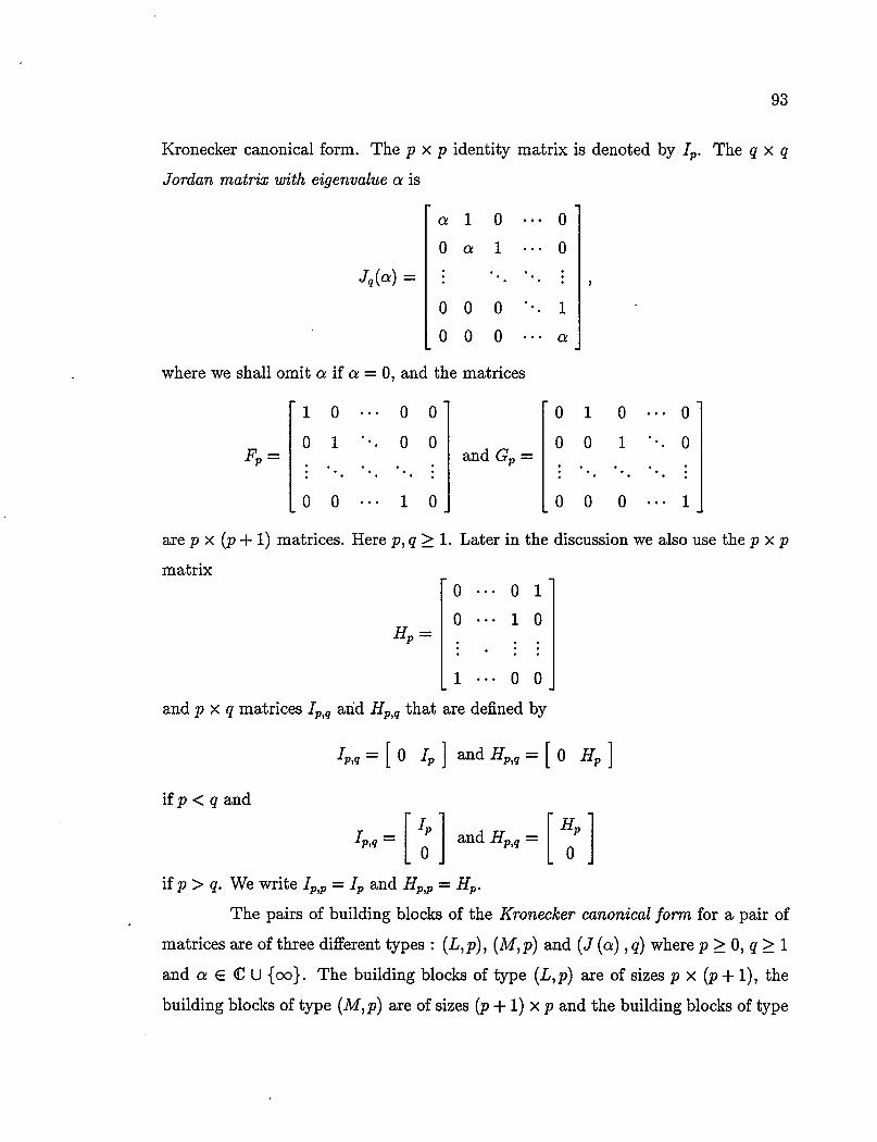
93
Kronecker canonical form. The p x p identity matrix is denoted by I. The q x q
Jordan matrix with eigenvalue a is
Jq(a) =
alO ...
0a 1••0
000 1
000 a
where we shall omit a if a = 0, and the matrices
10 00
01 00
00.• 10
and G =
010 0
001 0
00 0.•1
are p x (p + 1) matrices. Here p, q ≥ 1. Later in the discussion we also use the p x p
matrix 0...01
0...10
1...00
and p x q matrices 'p,, and Hp,q that are defined by
if p < q and
Ip,q [0 I] and Hp,q [0 H]
11 1H p,q = I, ] and Hp,q = 0
if p> q. We write 1p,p = I, and Hpp = H.
The pairs of building blocks of the Kronecker canonical form for a pair of
matrices are of three different types : (L, p), (M, p) and (J (a) , q) where p ≥ 0, q ≥ 1
and a E C U loo}. The building blocks of type (L,p) are of sizes p x (p + 1), the
building blocks of type (M, p) are of sizes (p + 1) x p and the building blocks of type

94
(J (a) , q) are of sizes q x q. Here the blocks of types (L, 0) and (M, 0) which are of
'sizes' 0 x 1 and 1 x 0, respectively, correspond to a column of 0's and a row of 0's,
respectively, in the Kronecker canonical form. Suppose that p ≥ 1. Then the pairs of
building blocks and the corresponding types are:
(Fr, G), type (L,p),
(G, F'), type (M,p),
(I, J, (a)), type (J (a) ,p)
if a E C, and
(Jr, I), type (J(oo),p).
The theorem of Kronecker (cf. [85, p. 37] or [92, Theorem A.7.3]) states that every
pair of m x n complex matrices (A, B) is equivalent to a pair of matrices in block
diagonal form with diagonal blocks of types (L, p), (M, p) and (J (a) , q). We call
this block diagonal form the Kronecker canonical form of a pair (A, B). We call the
collection
1= {(L,ll),...,(L,lPL);(.AII,ml),...,(ivl,mPM );(J(al),jl),...,(J(aPJ),jPJ);}
of the types of the diagonal blocks the set of invariants of a pair (A, B). The elements
of the set I are called the invariants. It is a consequence of the theorem of Kronecker
that two pairs of m x n matrices (A, B) and (C, D) are equivalent if and only if
they have the same sets of invariants. See [85, Theorem 5, p. 40] or [92, Corollary
A.7.4]. Note that in our discussion we view the initial u x v block of zeros in [92,
Theorem A.7.3] (in [85, expression (34), p.39] this is the initial h x g block of zeros)
as a collection of u blocks of type (L, 0) and v blocks of type (M, 0). This enables us
to absorb the initial block of zeros into the blocks of types (L, p) and (M, p).

95.
Example 3.2 The pair of matrices
/ 100 000
001
000
0 0 0
000
000
000
100
010
Th 1 0 0 0 0 \ 001000
, 0 0 0 0 0 0
000210
_0 0 0 0 2 0_j
has the set of invariants I = {(L, 0), (L, 1), (M, 1), (J (2) , 2)} and the pair of ma-
trices / 0000
0000
0000
0010
\0 0 0 1
0 0 0 0
0000
0 1 0 0
0001
0000 I
has the set of invariants I = {(L,0) , (M, 0), (M, 0), (J (0), 2), (J (co) , 1)}. 0
Example 3.3 Suppose that Al and A2 are commuting nilpotent N X N matrices,
that they are brought to the form (1.2) and furthermore, we have kerA2 = CN. (Here
we use the notion introduced in Section 1.2.) We can further assume that the row-
cross sections R', j E r0 are linearly independent and R30' = 0, j = ro + 1, r0 +
2, . . . , do, where ro is the dimension of the subspace of 2 x d1 matrices spanned by
R?', j E d0. Then we write
0 A°' A=
1.0 0 ]' where has dimensions ro x d1 x 2, and A°' = (A?', A2°'). Suppose that (.?', ') is the Kronecker canonical form of the pair (A?', A1) and that matrices P and Q
are such that
= PAQ and = PA IQ.
Then the array UAU1 = [0 o1]
00 where U --
P 0 0
010 fBol
0 0 Q-'
and =

96
(ñ1, 1) , is a canonical form for the pair of commuting matrices A1 and A2. We
remark that for similar, and also for more general, pairs of commuting matrices a
canonical form is given by Ge1'fand and Ponomarev in [86, Chapter II]. 0
Next we introduce the notion of Kronecker basis for a pair of matrices (A, B).
With every invariant in t El we associate a Kronecker chain C of linearly independent
vectors as follows
Ift=(L,p) then CL={ul,iEp+1} and
Bu1 = 0,
Bu1 = Au1_1, i=2,3,...,p+1,
0. = Au,,+1.
Ift=(M,0) then CL.=O and ift=(M,p),p≥l then CL={ul,iEp} and
Bu1 = Au1_1, i=2,3,...,p.
Ift.=(J(cr),p),ctEC, then C,={u1,iEp} and
(cA — B)ui = 0,
(aA—B)u1 = Au1_1, i=2,3,...,p.
And finally, if t = (J (oo) ,p) then C = {u, i Epj and
Au1 = 0,
Au1 = Bu1...1, i=2,3,...,p.
The union of all Kronecker chains of a pair of matrices (A, B) is called a Kronecker
basis of (A, B).
Remark. Note that if (C, D) is the Kronecker canonical form of a pair of matri-
ces (A, B), and the matrices P and Q are such that relation (3.5) holds, then the
columns of the matrix Q4 form a Kronecker basis of (A, B). They are partitioned
into Kronecker chains according to the sizes of diagonal blocks of the canonical form
(C, D). Note also that if m = n and A = I then the notions of Kronecker canonical
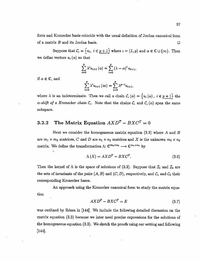
97
form and Kronecker basis coincide with the usual definition of Jordan canonical form
of a matrix B and its Jordan basis. 0
Suppose that C = {u, i E p + i} where L = (L,p) and a € C U fool. Then
we define vectors u (a) so that
>2 A1u+1 (a) = (A - a)1uj+i,
if a E C, and
A1u 1 (oo) = >2 Au1+i,
where A is an indeterminate. Then we call a chain CL (a) = {u1 (a), i E p + i} the
a-shift of a Kronecker chain CL. Note that the chains CL and CL (a) span the same
subspace.
3.2.2 The Matrix Equation AXDT - BXCT = 0
Next we consider the homogeneous matrix equation (3.3) where A and B
are m1 x m2 matrices, C and D are n1 x n2 matrices and X is the unknown m2 x n2
matrix. We define the transformation A: C2 xn2 Cml xnj by
A (X) = AXDT - BXCT. (3.6)
Then the kernel of A is the space of solutions of (3.3). Suppose that _Tj and 12 are
the sets of invariants of the pairs (A, B) and (C, D), respectively, and C1 and C2 their
corresponding Kronecker bases.
An approach using the Kronecker canonical form to study the matrix equa-
tion
AXDT - BXCT = E (3.7)
was outlined by Rózsa in [144]. We include the following detailed discussion on the
matrix equation (3.3) because we later need precise expressions for the solutions of
the homogeneous equation (3.3). We sketch the proofs using our setting and following
[144].

98
Suppose that 11 E Ii and 12 E 12 and that C1L1 and C22 are the corresponding
Kronecker chains. Now we define a set Y of pairs of invariants (ti, 12) e Ii x 12. A
pair (11, 12) is in the set Y if one of the following holds
(1) t = (L,pi) and 12 = (L,p2),
(ha) 11 = (L,pi), 12 = (M, P2) and Pi <P2,
(fib) bl = (M,p1), 12 = (L, P2) and p > P2,
(iiia) 1 = (L,pi) and t2 = (J (a) ,p2),
(hub) b, = (J(a) ,pi) and 12 = (L, P2) and
(iiic) t = (J (a) ,pi) and £2 = (J (a) ,P2).
Then we associate with a pair of invariants
matrices as follows
(11, 12) E J a set A( 112) of
(i) if 11 = (L,pi), 62 = (L)p2), C1 1 = {u1, i E P1 + i} and c2 = {u21, i E P2 + i}
then
= {Ai; A1 = E 1 E Pi +P2 + ii+i2=l+1
(iia) if tj = (L,pi), 12 = (kf,p2), where pi < P2, C11 =
= {u2, i e P2} then
= {Ai; Al = P1
u1,p1+1i+l, i=O
1
iEpi+1} and
(fib) if 11 = (M,p1), 12 = (L, P2), where Pi > P2, C1 l = {u1, i E pi}
{u21, i E P2 + i} then
A(L1,L2) = Al; Al = 2,p2+1—i' 1' 1 E Pi - P2 i=O
and C2 2 =

99
(iiia) if t1 = (L, pi), t2 = (J (a) ,p2), where a E C U fool, C11 (a) = {u1 (a), i E
Pi + i} is the a-shift of the Kronecker chain Ci 1and c22 = {u2, i € P2} then
= Al;-Al = u1 1 (a) U2i2, 1 € P2}; ii+i2=l+1
(iiib) if t1 = (J (a) ,pi), where a E C U fool, t2 = (L, P2), Ci1 = {u11, i E p, and
C2L2 (a) = {u21 (a), i E P2 + i} is the a-shift of the Kronecker chain C22 then
= Al; Al = u1j1u2j2 (a), 1 € Pi} +i2=1+1
(iiic) if t1 = (J (a) ,pi), L2 = (J (a) ,p2) , Ciq = {u11, i € pi} and C2 2 = {u21, i E
P2} then
= Al; Al = Lu liu2,p2 i+1 i=1
1€ min {P1P2}}.
Using the above setting we have the next important result.
Theorem 3.4 A basis A of the kernel kerA, i.e., a basis for the space of solutions of
the matrix equation AXDT - BXCT = 0, consists of the union of all the sets A(Ll,2)
for pairs of invariants (4, t2) in the set J.
Proof. Suppose that (As, B') and (C', D') are the Kronecker canonical forms
of the pairs (A, B) and (C, D), respectively, and that there are invertible matrices
P, Q, R and S such that
A = PA'Q, B = PB'Q, C = RC'S and D = RD'S. (3.8)
Then equation (3.3) is equivalent to the equation
A'X' (D1)T - B'X' (Cl)T = 0, (3.9)

100
where X' = QXST. Because the matrices A', B', C' and D' are block diagonal,
equation (3.9) becomes a collection of equations, one for each pair of invariants t1 E Ii
and L2 E 1 2. The invariants ti and t2 are of three different types. So we would have
to consider nine different cases but because of the symmetry we only need to consider
six different situations. We write Y for a block of the unknown matrix X in each of
the cases considered
(a) If t1 = (L,pi) and t2 = (L,p2) then we have the equation
F1YG T - G 1YF =0. (3.10)
Then a direct calculation shows that the matrices in the set
A'( 1,2) = IJlHp,+j,P +1, 1 E P1 +1; H1•1,1 (j, )T ' } (3.11) solve (3.10). They are linearly independent. By a dimension argument it follows
that the set (3.11) is a basis for the space of solutions of (3.10).
(b) If t1 = (L,pj.) and t2 = (M,p2) then we have
F1YFJ, - GP1YGZ =0. (3.12)
If Pi ≥ P2 then this equation has the only solution Y = 0. If P1 <P2 then the
set
4142) = {Hp1 +i,p2J 1, 1 E P2 - Pi}
is a basis for the space of solutions of (3.12).
(c) Suppose now that tj = (L, p1) and t2 = (J (a) ,p2). Using the a-shift Cl,, (a)
instead of Cl,, we may assume without loss that a = 0. So we suppose that
tj = (L, pi) and t2 = (J (0) ,p2). Then we have
and the set
F YJT_GY0 (3.13) P1 ...... P2
= I H1•1 (z_i\T E Za} P2)
is a basis for the space of solutions of (3.13).

101
(d) If t1 = (M,pi) and £2 = (M,p2) we have
FYGP - GYF1, =0.
This equation has no nonzero solutions.
(e) If t = (M, pi) and 12 = (J (a) ,p2) then we have
FTYP1 7P2 (a)T _G y PT GY =0.
This equation also does not have a nonzero solution.
(f) Finally we consider the case tj = (J (a) ,pi) and 12 = (J (/3) ,p2). First suppose
that a,,3:0 oo. Then we have
(3.14)
If a 54 /3 then this equation has the only solution Y = 0. If a = /3 then the set
4142) = {JLuI1,, 1 E min {pi,p2}} (3.15)
is a basis for the space of solutions of (3.14). Similarly it follows that there is
no nonzero solution when a 54 /9 and either of a, /3 is oo. If a = = oo then
the set A1,2) is as above in (3.15).
, By definition we have that X = Q -'X ' (S_1 T . . The columns of the matrices
Q' and 5' form Kronecker bases for (A, B) and (C, D), respectively. Then it follows from (a) that the set A( 1,L2) defined in (i) is a basis for the subspace of solutions of
the equation (3.3) associated with a pair of invariants tj E 11 and 12 E 12 of types
11= (L,pi) and 12= (L,p2). Similarly, it follows from (b) that the sets A(Ll,L2) of (iia)
and, by symmetry, also of (iib), span the subspaces of the equations associated with
the corresponding pairs of invariants. Case (c) implies a similar conclusion for the sets
of (iiia) and (iiib), and case (f) implies a similar conclusion for the set of (iiic). Then
it follows that the union A of all the sets A( 1,2) corresponding to pairs of invariants
(ti, 12) e J form a basis for the space of solutions of the equation (3.3) and therefore also a basis of the kernel ker A. 0
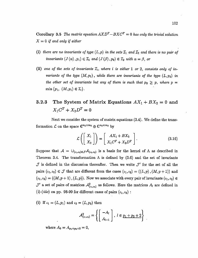
102
Corollary 3.5 The matrix equation AXDT_BXCT = 0 has only the trivial solution
X = 0 if and only if either
(i) there are no invariants of type (L, p) in the sets 11 and 12 and there is no pair of
invariants (J(a),pi) E 1 and (J(/3),p2) E 1 with cr=fl, or
(ii) one of the sets of invariants Z, where i is either 1 or 2, consists only of in-
variants of the type (M,pi), while there are invariants of the type (L, P2) in
the other set of invariants but any of them is such that P2 ≥ p, where p
min {pi, (M, pi) E Z}.
3.2.3 The System of Matrix Equations AX, + BX2 = 0 and
X1CT+X2DT = o
Next we consider the system of matrix equations (3.4). We define the trans-
formation £ on the space ED Cfl2Xm2 by
AX, +BX2
X2 ) X1CT+X2DT (3.16)
Suppose that A = U(L1,L2)Ej-A(1,2) is a basis for the kernel of A as described in
Theorem 3.4. The transformation A is defined by (3.6) and the set of invariants
J is defined in the discussion thereafter. Then we write J' for the set of all the
pairs (t1, t2) E J that are different from the cases (t1, t2) = ((L, p) , (M,p + 1)) and
(4, t2) = ((M,p + 1), (L, p)). Now we associate with every pair of invariants (4, 12) E
a set of pairs of matrices A 1,2) as follows. Here the matrices A1 are defined in
(i)-(iiic) on pp. 98-99 for different cases of pairs (ti, 12)
(i) If tj = (L,p1) and 12 = (L,p2) then
(I—A11
where A0 = A 1+,,2+2 = 0,

103
(ii) If tj = (L, pi), 12 = (M,p2) and Pi + 2 ≤ P2 or tj. = (M,pi), 12 = (L, P2) and
P1 ≥ P2+ 2 then
A1,2) I -Al JP1 —P21
1 = Li
(iii) In cases (iiia), (iiib) or (iiic), if a € C, then
(1
1 Al LAi+A1_' A(,, 12) = - 1 E
where p = P2 if t = (L, pi) and 12 = (J (a) ,p2), p = p' if 11 = (J (a) ,Pi) and
12 = (L, P2) and p = min {pi,p2} if ti = (J (a) ,pi) and 12 = (J (a) ,P2). Here
we write A0 = 0. If a = oo then
Al-1 EP C(112) { [ 1 =
A1
where p is defined as above and A0 = 0.
In the above setting we have the following result:
Theorem 3.6 The kernel of £, i.e., the space of solutions of the pair of matrix
equations AX1+BX2 = 0 and X1CT+X2DT = 0, has a basis A2 = U(LI,L2)ey'A lL2),
where the sets Al,L2) are given above.
Proof. Let the matrices A', B', C', D', P, Q, R and S be as in the proof of
Theorem 3.4. We write X = QXST for i = 1, 2. Then X1 € ker £ if and only if X2

104
in the proof of Theorem 3.4. We write Y1 and Y2 for the blocks of X1 and X2,
respectively, considered in each of the cases. First we have the case tj = (L, pi)
and t2 = (L, P2). Then we write Y1' = '!i'' 'y1A and Y = 'i ' öJA'Y, where = 1 E pi + 1 and A = H1•1,•1 (j11_1 )T I = + 2,Pi +
3,. . . ,pi + P2 + 1 are the elements of the set A1,2). It follows from the equations
(3.17) that -y + i+i = 0 for 1 E Pi + P2. Thus the set
A 21 { I ] = lEPi+P2+2}
A 1
where A'0 = = 0, is the basis of the block of the equations (3.17) correspond-
ing to the pair of invariants (ti, 12). Because the columns of the matrices Q-1 and
S' form Kronecker bases for the pairs (A, B) and (C, D), respectively, it follows that
as defined in (i) above, form the basis of the subspace of ker £ corresponding
to the pair of invariants (ii, 12).
Using the same method as for the case tj = (L, p1) and .62 = (L, P2) above,
we prove that the sets Al2) in cases (ii) and (iii) form bases for the corresponding
subspaces of ker £. Then the proof is complete. 0
Now we define a mapping ij on the set of pairs of invariants J' by
?7 (11, 12
(L,pi+p2+1),
(M, P2 - P1),
(M, P1 - p2),
(J (a) ,P2)
(J(a),pi),
(J (a) ,min {pi,p2}),
if
if
if
if
if
if
is as in (i),
is as in (iia),
is as in (iib),
is as in (iiia),
is as in (iiib),
is as in (iiic),
(3.18)
where the cases (i)-(iiic) are defined on page 98. Then the set of invariants I =
{ii (ti, 12), (ti, 12) E J'} is called the set of invariants of the kernel of L. We write
= A,,L2) if I = i (ti, 12). We will use the set of invariants I and the corresponding
basis A2 = UEIA to describe a special basis of the second root subspace of the
two-parameter system.

105
3.2.4 Remark on the Matrix Equation AXDT - BXCT = E
and Root Subspace for Two-parameter Systems
Let us now consider a particular eigenvalue A = (A1, A2) E o (W). Then we
write
T2=W1(A)=—V,o-i-A1V,1-i-A2V2 for i=1,2.
From the properties of determinantal operators in Lemma 2.1 it follows that
and
A2z02 —V11 ØT2—T1®V21.
Again we view the above transformations as acting on the space of n1 x n2 complex
matrices. Suppose that X0, X1,... , X, E CT ® tjJfl2 (identified with Cfh><n2 via the
isomorphism E defined by (3.2), only replacing ni for qj) form a Jordan chain for r1, i.e.,
(A11 - r1) x1 = x1_1
or equivalently
(A1zo - ) X = (3.19)
for j = 0, 1, . . , p and X_1 = 0. These are equivalent, via the isomorphism E, to the
recursive system of matrix equations
T1XV - V12XT" = V1X 1V - VX 1V. (3.20)
We have a similar system for the second associated operator r2. If X0, X1, X,, is its Jordan chain then
V11XT' - T1X V21 = V11X_14 - V12X_1V (3.21)
for j = 0, ,p and X_1 = 0. At every stage of this recursive system of matrix
equations we have to solve a matrix equation of the type
AXDT - BXCT = E. (3.22)

106
This equation can be studied using the Kronecker canonical forms for pairs (A, B)
and (C, D) similarly as for the homogeneous equation (3.3). For every type of a pair
of invariants we could give solvability conditions and a particular solution when it
exists. Then we could apply this result to the recursive system (3.20) (or (3.21)). We
would have to solve simultaneously the recursive system (3.20) and a similar system
corresponding to 3I - r. The weakness of the eventual procedure is that it would only give a basis for the root subspace for one of r1 (or 1'2) and would not necessarily give a basis for the root subspace ker (Al - T)N. In the procedure we would use ideas
developed in the theory of marked invariant subspaces in order to prove completeness
(see [72] and [73, Section 4.4]). We state the definition of a marked invariant subspace
below, but we do not develop the procedure in further detail.
Definition. A subspace Al C CN is called a marked invariant subspace for a trans-
formation A: 1yV . JN if A1 is invariant for A and if there exists a Jordan basis 5
for A on C' such that a subset of 5 spans X.
Marked invariant subspaces were introduced in [92, Section 2.9]. For further
developments see [46, 47]. An earlier related disposition was given by Cater in [53,
Lecture 4-3] where he proves a finite-dimensional version of results of Vilenkin [165,
pp. 102-106] and Kaplansky [116, Chapter 18].
3.3 A Special Basis for the Second Root Subspace
of Two-parameter Systems
We saw in the previous section that we can build a natural basis for the
kernel of £ from Kronecker bases of the pairs of matrices (A, B) and (C, D). This
result can be applied to the kernel of the transformation V in the two-parameter case.
We use the setting of Subsection 2.5.2 with n = 2. A special basis for ker V can be
given using Kronecker bases for the pairs of matrices (v, 'ç), i = 1, 2. Suppose that
I, is the set of invariants of the pair (va, v) and C = UtECjL is the corresponding

107
Kronecker basis where Ci, is a Kronecker chain associated with the invariant i. E
We write I for the set of invariants of the kernel ker V and A for the subset of the
basis A2 of ker DO, corresponding to the invariant t E I. We described in Theorem
2.21 a correspondence between elements of a basis for ker (Al - F)2 / ker (Al - F) and
elements of a basis for the kernel of D. Therefore a special basis for ker DOA induces
a special basis for ker (Al - F)2. The exact correspondence is described later in this
section. We have three different types of invariants in the set of invariants I for the
kernel ker V. It will turn out that they correspond to the three different types of
invariants of a pair of matrices A°' = (A?1, A 1), as defined on page 92.
In the rest of this section we describe the construction of a special basis for
ker (Al - F)2 using the basis A2 for ker D. We discuss each of three different types
of invariants t E I separately.
3.3.1 Basis Corresponding to an Invariant t = (L,p)
Theorem 3.7 Suppose i = (L, p) = 77 (t1, 62) where z = (L, p1) E .I. and 62 =
(L, P2) E 12 and that C11 and C2L2 are the associated Kronecker chains. Then there
exist vectors x11 E H, i = 1,2 and li = 1,2,... ,p + 1 such that
and
The the vectors
and
io = W (A) x1,
ViX'o + V2xb = W (A) x for l= 2, 3, . ..
V12XPj4 = W (A) x.
k kç 1 ,, k+1—1 ZO_Z_1XiOX2O
1=1
z = (x 1 0 x' 1 + x0 ®
are linearly independent. It also follows that
kEp
k ep+l
(3.23)
(3.24)
(3.25)
(3.26)
(3.27)
(A11 - r1) 4 = 4 (3.28)

108
and
Ni \ k k—i - J. r 2) Z1 =
for kEp, where zoo =4=0 and x1=0fork<Oandk>p+l.
(3.29)
Proof. Suppose that C = {uk; k E p + 11 i = 11 2. Because i.j = (L, pi)
it follows from the definition of a Kronecker chain that
= 0,
= T/u i,i_i,
T/ - A - yiiui,pi+i
Then we have by a standard argument involving Lemma 2.12 that there exist vectors
x1 E H such that (3.23), (3.24) and (3.25) hold. We can construct vectors (3.26)
and (3.27), and then it follows that
and
k
1=1
Vjia40 V12x0 k+i—i TI k+1—1
v21X20 V 22 20
k
(1\2o - Li2) z =
V11x0
v2ix -i—i 20
1=1
V11x0
V21x' 1
Wi (A) x' 1
W2 (A) xt'' V12x0
TI k+i—i "22X20
V12x0 V12x0
V22x20 1 V22X20
V11x0 Wi(A)x 1
V21x'' W2 (A) 21
V11x0 V12x0 k—i k—i
2iX2o 22X20
0
0
for. k = 1,2,...,p. Hence (3.28) and (3.29) hold. Here we assume z00 - — zo - 0.
The vectors 4, k = 1,2, - . . ,p - 1 are linearly independent because the vectors
x, k = 17 2, ... ,pi are linearly independent. Then it follows from (3.28) and (3.29)
that the vectors {4; k E u {z; k E p + i} are linearly independent. 0
If we restrict the transformations A11—T1 and A2I- 2 to the joint invariant
subspace JV spanned by the vectors {4; k € p} u{4; k E p + i} then they commute

109
and we have
I0G1
[0 0 0 (All —ri)Ig= I and (A2I—r2)lg= I [ ]
Note that the invariant of the pair of matrices (Fr, G) is (L, p)
3.3.2 Basis Corresponding to an Invariant t = (M,p)
Suppose that t = (M,p) = i (ti, 62) where tj = (L, pi) E I, 62 = (M,p2) E
12 and p = P2 - Pi > 1, and that C1L1 and C2 2 are the associated Kronecker chains.
The basis for the case t 1 = (M, pi) E I, 62 = (L, P2) E 12 and P = Pi - P2 > 1 is
obtained symmetrically, interchanging i = 1 and i = 2.
Theorem 3.8 If 1. = (M, p) E I is as above then there exist vectors x E H, k =
1,2,... ,p + 1 (x 1 = x' = 0)such that
V11x0 = W1 (A) x1,
k=2,3, ... ,p
and
V12x1 = W1 (A)
Then the vectors
4=x 0®x, kEp+1, i=1,2, 1=1
and P1+l P1
= x1 0 x 11 + xo 0 xf' 1 ', k E p 1=1 1=1
are linearly independent. Furthermore, we have
(A11 - 1) z = (3.30)
and
Ni 112) z: = 4 (3.31)
for k E 2

110
Proof. The vectors x exist similarly as in the proof of Theorem 3.7 using
the definition of the Kronecker chains Cii, and Lemma 2.12. To prove the theorem
we need to establish relations (3.30) and (3.31). These follow by a straightforward
calculation
and
P1+l
(A10—z1)z=: > 1=1
Wi (A) x1
A) pi+k-1+1 W2 (
V11a40 V12x0 V2iX 1+II+l T t pi+k—l+1
20
(A2o -
V11x0 V11x0 tr i+k—l+1 TI pl+k—l+1 v21X20 V21 X20
= L0z.
TI 1 v12X10
i,22X2 p0i+k-1+1 v
0
V12x0 V12x0
V22x 1 V22x
W1 (A) X11, W2 (A) 21 pi+k_1+1
TI I v11X 10
V2jx'' 20
V12c40 TI pl+k—1 Y22X2O
0
0
Then we argue as in the proof of Theorem 3.7 to complete the proof. 0
If we restrict the transformations x1I—r1 and A2I- 2 to the joint invariant
subspace .A/ spanned by the vectors {4; k E p + 1 u {4; k E p}, described in the above proof, then we have
(A11—r1) I= 0 (F)T
00 and (A21 - r2) jg=
0 (G)T
0 0
Note that the invariant of the pair of matrices ((F) T, (G)T) is (M,p).
3.3.3 Basis Corresponding to an Invariant b= (J (a) ,p)
Suppose that t = (J (a) ,p) = ij(t1,t2) where t1 = (J (a) ,pi) E Ii, t2 =
(J (a) ,p2) E 12 and p = mm {pl,p2}, and that C1L1 and C2L2 are the associated

111
Kronecker chains. The basis for the case tj= (L, p1) and 12 = (J (a) ,P2) is obtained
using the same arguments as in the case t = (J (a) ,pi) and 12 = (J (a) ,P2) using
the a-shift Cl,, (a) = {u (a) , i e Pi + i} and writing u11 (a) = 0 for i ≥ pi + 1 if
P2 > P1+l. The case tj = (J (a) ,Pi) and 12 = (L, P2) is analogous, only interchanging
i = 1 and i = 2.
Theorem 3.9 If ti = (J (a) ,pi) and 12 = (J (a) ,p2) then there exist vectors Xk E
H, k = 1, 2,. . . ,p such that
U1 (a) xto = W1 (A) xti
and
Then the vectors
and
U(a)x+Vix' =W1 (A) x1 k=2,3, ... ,p.
k
4=Lxoøx' 1, kEp 1=1
4 = (x 1 ® x' 1 + x0 xt''), k E
are linearly independent and furthermore
(A1I - r1) 4 = a4 + 4' (3.32)
and
Ni - 1'2) 4 = 4 (3.33)
for k E p.
Proof. The theorem follows as the previous two given the relations (3.32)
and (3.33). These are established using a simple calculation:
k
(A1zo - ) 4 = l=1
Wi (A)
W2 (A) x21 1 '
V12x0 T k+i-1 V22X20
0

112
k
=>: l=1
and
U1 (a) xo V12x0
) k+1-I V22x'1 U2 (a x20
k
(A2zo - 2) z = 1=1
V1x0 U1 (a) x0
V2x20 '1 U2 (a)
V11x0 Vi2x'0 i, k-i TI k-i v21X20 v22X20
V1x0 Wi(A)a41
V2x' 1 W2 (A) 21
= aL.0z' + Loz 1
0
V11x0 k-i
21X20
0
= AO ZOk.
0
If we restrict the transformations A1J—T1 and A2i—F2 to the joint invariant
subspace Al spanned by the vectors {4; k E u {4; k E P1 given in the above proof. Then we have
l (A11—r1) = o JP (a)
to o ] and (A21 - r2) kr 00
54
The invariant of the pair of matrices (J (a) , I) is (J (a) ,p).
Suppose that for every element in the set of invariants I of the kernel of
we construct vectors 4 and z as explained in the proofs of Theorems 3.7-3.9. Note that they are linearly independent. We denote the set of these vectors by
1% and by Al' the subspace they span. The linear transformations (A11 - F1) and
(A21 - I'2) restricted to the subspace Al = ker (Al - F)2 commute and are nilpotent.
Furthermore Al' C Al. If Al' Al we complete the set 5 by a set of vectors, say 13",
to the basis 52 for Al. We write Al" = £ (5"). Because the vectors z are as many as
dim ker V and are linearly independent it follows from Theorem 2.21 we can assume
that Al" c ker (Al - r). We write the pair of restricted transformation (A11 - r) ,
that are nilpotent and commute, in the form (1.2) using the basis 132. It follows from
Theorems 3.7-3.9 that the array A°' has the form
A A°' 01= 0
(3.34)

113
where
a101 ... 0
o a 01 0 ,.1
o •.. Q a 01 ,.1 +1 0i =
(tl
a; +r2 01 a,.1 +r2 +1
0
0
0
01 an +r2+r3
(3.35)
The first r1 blocks a1 in the array (3.35) correspond to the invariant (L, p) in the
set I, the next r2 blocks correspond to the invariants (M, p1) in the set I and the last
r3 blocks a1 correspond to the invariants (J (a) , ps). The rows of 0 at the bottom
in (3.34) are as many as there are vectors in the set Jsf". Note that the array A,
where A°' is in the form given by (3.34) and (3.35), is in a canonical form described
in Example 3.3. Note also that the set of invariants of the pair of matrices (A?', Ag') equals I.
To illustrate the preceding construction we discuss two examples.
Example 3.10 Consider again the two-parameter system of Example 2.22. The sets
of invariants for the pairs (vfjo, v1°) and (v2°, v2o) that correspond to the eigen-value A (0,0) are {(L, 0), (M, 0)} and {(L, 1), (M, 0)}, respectively. A Kronecker
chain that corresponds to the invariant (L, 1)is [] , []. The set of invariants for the kernel ker V"° is then { (L, 2) }. We find that vectors
0
xh=x,= 1
—1
are such that
and x1 =
0
0
0
9 ,x 1 =
1 2
V,ix,o = W, (A0) xi,, V,2x,0 = W1 (A0)
0
0
0

114
and
10 V22x0 = W2 (A0) 4, V224 - = W2 (A0) 4 and - V214 = W2 (A0) 4.
Then it follows from Theorems 2.21 and 3.7 that the vectors
1 0
o 1
o 0
o 0
0,0
0 0
0 0
0 0
0 0
0
0
0
1
0
0
—1
0
0
0
0 1 2
1
0
and
0
0
0
0
1
0
0
—1
0
form a basis for ker (Al - )2. Note that the above method to construct a basis differs
from the method given in the proof of Theorem 2.21 and used in Example 2.22, hence
also the bases constructed in the two examples are not the same. 0
Example 3.11 Suppose that we are given matrices
T1\11 - V -
1 0 0 0 0 0
010000
000000
000100
000010
000001
1 00 0 0
00000
0 0 1 0 0 and V22
00010
0 0 0 0 1
LrX , V12 -
010000
001000
000100
000010
000001
000000
0 1 0 0 0
00100
00000,
00021
0 0 0 0 2

115
and we write 'k for k x k identity matrix. Then we form a two-parameter system
and
W1 (A) = 16
A vii
16 0 TI
V 1 00 A2 -
0 '6 0
IOVlA+II5V2lA 1001 W2(A)L 0 j to 15 ] L15 0]
It follows from the structure of the above two-parameter system that it is nonsingular
and that A = (0,0) is an eigenvalue. We also find that the matrices Viit i,j = 1,2, are
the entries of the corresponding matrix DA if we choose x10 = [ y 0 10 = 16
16 0 = [] 0 and ,20 = 15 ] . Then { (L, 2), (M, 3) } is the set of invariants for 15 0
(v1, v1) and {(L, 1), (M, 1), (J (2) ,2)1 the set of invariants for (v2, v2). The set of pairs of invariants J' has three elements {(L, 2), (L, 1)}, {(L, 2), (J (2) ,2)1 and
{(M, 3), (L, 1)}. Applying the mapping 77 defined by (3.18) we find that the set of
invariants of the kernel of V is {(L, 4), (M, 2), (J (2) , 2)}. 0
3.4 Comments
Kronecker in [119] developed his canonical form as the answer to the prob-
lem posed by Weierstrass of finding a canonical form for a pair of bilinear forms.
The Kronecker canonical form is usually stated in terms of matrix pencils AA + B.
Because we use the Kronecker canonical form for a pair of matrices A°' = (Ag', A)
in a commutative array in the form (1.2), we have chosen to state it in terms of
pairs of matrices to keep in tune with our preceding discussion. For an early version
of Kronecker's result adapted to matrix pencils see Dieudonné's work [58]. We can
also find chapters on the Kronecker canonical form in recent monographs on Linear
Algebra, for example [85, 92]. This topic is also of current interest in various appli-
cations, e.g. in Control Theory (see [113, 125]), and various further developments

116
Van Dooren [61] gave a computational algorithm to find the canonical form, Atkinson
[11] extended it to a special class of tensors and Thompson [162] studied it for pairs
of self-adjoint matrices. The study of matrix and operator pencils AA + B and also
multiparameter pencils E AA1 + B motivated by multiparameter eigenvalue prob-
lems is found in several papers. For example, Blum [31], Fox, Hayes and Mayers [76]
and Hadeler [98], considered numerical methods to find eigenvalues of these pencils,
and Binding [22] gave a canonical form for self-adjoint operator pencils A..\ + B on
Hilbert space. Also Bohte in [36] studied numerical methods to calculate eigenvalues
of a two-parameter system of pencils.
The matrix equation AXDT - BXCT = E has been studied for a long
period of time (see [156, 157, 171]). The special cases XD - BX = E and also
AXDT - X = E have been thoroughly examined. See [128, Chapter VIII] for early
references, some later works being [107, 142, 145, 173]. In [143] Roth gave conditions
for existence of a solution of XDT—BX = E. Different proofs of his results were given
later in [74, 102]. The authors in [100, 101, 120, 123, 124, 127] suggested different
approaches to find explicit solutions of XD - BX = E. This matrix equation is
associated through Roth's results with extensions of block matrices [114, 174] and
with the Kronecker sum 10 D - B ® I. The latter was already known to Sylvester
(he calls it 'nivellateur') in [156], see also [13, 14, 126]. Eigenvectors and root vectors
for the Kronecker sum were given by Trampus in [163]. See also [132, Section 1.2] for
a thorough presentation.
The applications of these matrix equations are diverse. Barnett and Storey
in [14] discussed problems in stability theory where the equation XD - BX = E
arises. Epton [63] gives an example of a numerical method for implicit differential
equations where solving the equation AXDT - BXCT = E is essential. See also
[17, 127] for some other applications. The general equation AXDT - BXCT = E was
studied in [54, 63, 103]. Chu [54, Theorem 1] gave conditions for existence of a unique
solution. He also proposes a numerical algorithm to compute this solution. The idea
to use the Kronecker canonical forms of two pairs of matrices (A, B) and (C, D), in

117
order to solve this matrix equation, was brought forward by Rózsa in [144].
Two-parameter spectral problems were considered since the early days of
Multiparameter Spectral Theory. For example, two-parameter oscillation theorems
were proved by Klein [117], Bôcher [32, 33, 34] and Richardson [141]. Dixon [59]
studied expansions of functions in terms of eigenfunctions of a pair of coupled two-
parameter differential equations of Sturm-Liouville type. Also Camp [48, 49] and
Doole [60] proved various two-parameter expansion theorems. Fell [138] studied a
two-parameter system of integral equations of Fredholm type. In the 1950s Cordes
[55, 56] developed an abstract Hubert space setting for a special class of two-parameter
spectral problems (cf. also [131] for a modern presentation of Cordes's work). Later
Arscott considered particular classes of two-parameter spectral problems in [5, 7].
Among recent publications we find work of Binding, Browne, Faiermau, Isaev, Sed-
dighi and many others. Most of the early references discuss the right definite case
where eigenvectors alone are complete, while Binding and Browne [26] consider the
dimensions of root subspaces for general eigenvalues of self-adjoint two-parameter
systems.
118
Chapter 4
Bases for Root Subspaces in
Special Cases
4.1 Introduction
In this chapter we study the finite-dimensional completeness problem, i.e.,
the problem of finding a basis for root subspaces, for special cases of eigenvalues of
multiparameter systems.
In the second section of this chapter we consider nonderogatory eigenvalues.
Theorem 4.4 is the main result in this case. The method used to prove this result is in
part different from the method used to prove the completeness result for simple eigen-
values and can not be directly generalized. When an eigenvalue A is nonderogatory
the restricted transformations Ai = (AI - r.) Ik(AI r) N i E_ , that are commuting
and nilpotent, are assumed to be in upper Toeplitz form. With corresponding root
vectors we associate monic matrix polynomials. It turns out that the n-tuples of the
first row of the array A, consisting of matrices A•, i E n, form Jordan chains for these
matrix polynomials. A chain of vectors x0, x1,. . . , x, is a Jordan chain for a matrix
polynomial L () at an eigenvalue Po if
for k=O,1, .... p. (4.1)

119
(For further definitions concerning matrix polynomials see [89, 90].) We also give an
algorithm for the construction of a basis for a root subspace. As an application we
consider self-adjoint multiparameter systems. We obtain a new result for the real
simple eigenvalues of weakly-elliptic multiparameter systems.
Our main results are Theorem 4.18 and Algorithm 4.19 in the third section.
We use the same ideas as we did in Section 2.5 when we constructed a basis for the
second root subspace. We use essentially one more important fact, that we can sep-
arate for all i the kernels of the matrices W (A) and subspaces spanned by vectors
Xk, for k ≥ 1, that are used in the construction of root vectors in addition to the
vectors x0 E ker W (A). We ensure this by choosing vectors xg from a direct com-
plement H C Hi of ker W (A). This fact is used along with relation (2.7) to obtain
equalities of type (4.26). The matrix Sm plays a role similar to that of the matrices
B0 and DOA before. It acts on a space isomorphic to the space spanned by matrices
T(l,m_l), f E dm. These were the matrices introduced in Section 1.5. The matrices
T7(hlm_l), f E dm are linearly independent and their isomorphic images are elements
of the kernel of Sm. Next we can associate with every element in the kernel of 8m an
m-th root vector that is not an (m - 1)-th root vector. Our proof that this vector is
actually a root vector is technically very complicated. We do this in Lemma 4.17. We
also prove that we can associate in the same fashion a set of linearly independent root
vectors with a basis of the kernel of Sm. We prove by induction that this procedure
gives a basis for the root subspace. In the first subsection we establish a basis for
the third root subspace and in the second subsection we prove the inductive step. In
the third subsection we give Algorithm 4.19 and consider the special case of simple,
completely derogatory eigenvalues. Simple eigenvalues in the two-parameter case are
always completely derogatory. We also discuss the relation between our expressions
for the root vectors for simple eigenvalues of the two-parameter system and the con-
jecture of Faierman [69, Conjecture 6.1] on the structure of root functions for a class
of Sturm-Liouville boundary value problems (0.1).

120
4.2 Nonderogatory Eigenvalues
In this section we assume that A E o (W) is a nonderogatory eigenvalue.
The next result is a well known biorthogonality property between right and left Jordan
chains. We write it in the following form for future reference. We assume that index
i is fixed.
Definition. A Jordan chain z0, z1,. .. . z, (as in 0.2) is called maximal for a linear
transformation V at an eigenvalue Ao if zp 7Z. (A01 - V).
Lemma 4.1 Suppose that z0, z1,... , z, is a maximal Jordan chain for ri at the eigen-value Ai and w is a left eigenvector at the same eigenvalue. Assume also that
dim (ker (Ai I—r)) = 1. Then it follows that WO*L.OZk = 0 fork = O,l,...,p— 1
and woz 54 0.
Proof. For k < p - 1 we have 0 = w (A0 - j) zk+1 = w O*LOZk. Sup-
pose now that wJ.oz = 0. Then it follows that Loz E (ker (Ao - )*).L =
7Z (Az0 - j) and so there is a vector such that (A11 - r) = zr,. This
contradicts the assumption that z0, z1,... , z, is maximal Jordan chain. The proof is
complete. 0
In this section we will denote the family of multiindex sets
{(i1i2...in); 0≤j, -ii = k} (4.2) i=1
by Wk for k = 0,1,.. . ,p. Here p is a fixed nonnegative integer.
Lemma 4.2 Let {. = {b]. ,k = 021,... 2P} be a set of matrices and assume 13 2,21
that rank(Bo) = n - 1. Choose a vector x0 E ker (B0) \ {0}. Then there exist vectors x,i = l,2, ... ,p such that Ej=o Bjxi-j = 0 for = 1, 2,...,p if and only if
jEWs
b',', V1'2 b3
b22 b22 22 21 22 V2n
=0 (4.3)
i..:in iJn i1fl t1nl Vn2 (P

121
for i=1,2,...,p.
Proof. We construct a matrix polynomial
L (1k) = Ip' + BppP + B_1p"' +• + Bo = [b ()] i,j=1
Then
L(k) (0)=k!.Bk, k=0,1, .... p (4.4)
and because dim (ker L(0)) = 1 the polynomial L (p) has only one elementary divisor
at p = 0. Then by [90, Corollary 1.14, p.35] it follows that p = 0 is a root of degree p + 1 for the scalar polynomial d (p) = det L (/2) if and only if matrix polynomial
L (p) has a Jordan chain x0, x1, . .. , x, of length p + 1 at p = 0. That is, if and only
if the vectors x0,x1,. . . ,x,, x0 0 0, are such that
-L() (0) Xk_ = 0,
or if we use (4.4), if and only if
k
= 0,
for k=0,1, ... ,p, (4.5)
for k=0,1,...,p. j=0
If the polynomial d (p) hasp= 0 as aroot of degree p+1 then d(0) =d'(0)
d" (0) = 0. Finally the relations
d(k) (0) = , .
jE'I'k ii• 32. in.
=k! jE'I'k
b 1) (0) b(0) (.1) 01n (0)
b2) (0) b) (0) '(22) O2 (0)
bj (0) b;) no (0) (0)
11 12 "in
b32 b22 b22 21 22 2n
ljn tin 1,.in 'n1 -'n2
hold and the result follows. 0

122
The above lemma is used in the proofs of the main results in this section
concerning bases for root subspaces for nonderogatory eigenvalues. For the definition
see page 78. Let us recall that H C Hi is a direct complement of the kernel of W (A).
Proposition 4.3 Assume that the eigenvalue A E 3Y' is nonderogatory. Then the
following statements are equivalent:
(i) There exist n-tuples a1, a2,... , a, E C", a1 0 and vectors x1, x2,. .. , x1 €
Hill i=l,2,...,n such that
k-i
E U (a,_) xij = W (A) Xik 5=0
for k=1,2,...,p; i=1,2,...,n. (4.6)
(ii) There exist n-tuples ai,a2,...,ap E C", a1 34 0 and vectors 5i1,5i2, ..., xi, p..i E
H, i = 1,2,...,n such that
k-i
EyoUi(ak_j)xij=O for k = 1,2,...,p; i=1,2,...,n. j=0
(iii) There exists an index h such that dim ker (AhI - Th) = 1 and rh has a Jordan chain of length p + 1 at eigenvalue -Ah,
(iv) There exists a set of linearly independent vectors {z0, zj,. . . , z} C H such that
(AjI — FI)zk = Et'a1,k_5zJ fork = 0, 1,...,p; i = 1,2,...,n and not all ail = 0.
Proof. If we multiply (i) by y, on the left then (ii) follows. Assume now that
(ii) holds. In Proposition 2.15 we have already proved that (i) and (ii) are equivalent
for k = 1. Suppose now that we have already found vectors xj, x2,. . . ,x, ki, where
0 ≤ k <p, such that (4.6) holds. Then E:j U (ak_J) x; is orthogonal to the kernel
ker W (A)* and so it follows from Lemma 2.12 that there exists a vector 5 1k E H
such that E U (ak_J) xj = W (A) 5 ik. We can continue this procedure until k = p.
Therefore (i) follows.
It is easy to observe that (iv) implies (iii).

123
Suppose now that (i) holds. We define vectors
Zk = EX1j1 0 X2j2 & 0 Xflj
jEWk
for k = 0, 1,. . . ,p. It follows then from (i) and Lemma 2.1
= jE1Ik
n 3q1 = E E E aj,_i
j€Wk q,r1 'q=°
=
•ri•t V11
TTt "21
V1,i—lxljl
V2,1_1x252
Vn,i-lxnin
V11_1 W1(A)t V11
V_1 W2 (A) V21+1
V_1 W (A)t Vt ... Vt z+1 fin
il — i
E U1 (a12 _i) a.; 111 li=O 22-1 Fa U2 (a 2_,2) x212 12=0
Vi,1+1x111
V2,+ix2a2
in - 1 E U, (a1 _i) x,a, Vn,j+ixnj, in =0
V1,i-1x111
Vq_i,i_iXq...i,jq_i
Vq,i_ixqjq
Vq+1,i._1Xq+i,jqi
Vn,i-lxnjn
0 Vi,+ixi11
0
Zk =
Vq_i,i+ixq....i,jq_1
Vqrx gig 'l/,i+1X QIq
h1'q+1,i+1Xq+1,jq1 0
0
0 Vlnxljl
V2 x212
Vflnxnjn
(4.7) 0
(4.8)
In the displayed determinant (4.8) the first i - 1 and the last n - i - 1 columns
are the same as in the determinant displayed in (4.7). The vectors VqrXqjq , r =
1,. .. , i - 1, i + 1,. . . , n, in (4.8) can be substituted for Vgrxqiq without changing the

124
determinant. The sum (4.8) is then equal to
Vli,i_i 0 V11 1 ... Vltn
fl
>i: E E a_i9,, jEWk q,r=l 1q°
u 'nti
t A Vt Vt n,i+l • nfl
xljl 0 •• ® Xq_l,jq_lXqlq 0 0 • 0 (4.9)
For every multiindex j E 1Ji, where 1 < k, the vector x1j, 0 x22 0 0 x1 appears
exactly n times in the summation (4.9), once for every q = 1,2, . . . , n. Then we sum
in (4.9) over q and because a determinant with two equal columns is zero it follows
that the sum (4.9) equals
k-i
ak_I,
I=OjEW
Vix11 V12x111
V21x22 V22X2J2
V1 x111
V2 x252
0
k-i
= E ak._1,1I.oz1. j=O
This establishes (iv).
To complete the proof we will show that (iii) implies (ii). This implication
was proven in Proposition 2.15 for k = 1. Assume now that we have already found
a1,a2,. . . ,ak_i and . . i = 1,2,... ,n where k ≤p such that
i-i
l=1,2,...,k-1. (4.10) j=o
It remains to show that we can also find ak and Xi,k.i, i = 1,2,. .. , n such that
k-i
= 0-j=0
Since (i) and (ii) are equivalent we can find Xi,k_i, j = 1,2,.. . , n such that
k-2
E U (ak_2) xij = Wj (A) j=o

125
Next we build the vectors z1 = EJEW, x1j1 0 x2j2 0 ... 0 x,,, 1 = 0, 1,. .. 'k- 1. In
the proof of Proposition 2.15 we showed that
z1 E ker(AI—T)2/ker (Al —T).
In the Remark following that proof we pointed out that alh 0 0 for some h E 11. The
same calculation used to show that (i) implies (iv) also proves that (A11 - r) zi = E'0ai_j,z3 1= 0,1,...,k-1. Then the vectors ur = r lrzk_l, r = 0,1,...,k-1
form a Jordan chain for rh of length k (<p + 1). Because dim ker (AhI - rh) = 1,
every Jordan chain can be extended to a maximal one (cf.[92, Theorem 2.9.2(b), p.
85]). Lemma 4.1 implies that wL.0u1 = 0,1 = 0,1,— , k - 1 and then, because
£({ui; 1= 0,i,...,k—i}) = £({zj; l=0,1,...,k-1}) = ker(AhI—rh)', it also
implies that
WO* ozi — , 1 = 0,j.,...,k -
Next we form the n x n matrices B1 = 1 = 0, 1,.. . , k—i where = yV11x11.
-7 ij=11The relations (4.10) are equivalent to E'O Baj_1 = 0 for 1 = 1, 2,. . . , k - 1 and the
relations (4.11) are equivalent to
=0, for l=0,1,...,lc-1. JEW,
Since A is nonderogatory rank B0 = n - 1 and then Lemma 4.2 implies that there
exists an n-tuple ak such that E1 BJak_ = 0 or, equivalently, such that
k-i
yj*O Ui (aA;-j) Xij =0 j=0
for i=1,2, ... ,n. 0
Remark. Suppose that the conditions of Proposition 4.3 hold. Then for every index
h such that aih 0 0 (there is always at least one such h because a1 0) the vectors
UI = (AI - rh) 1 zp, 1 = 0, 1,. . . ,p form a Jordan chain for rh at eigenvalue Ak.

126
This implies that the vectors z0, z1,. . . , z, are linearly independent and they span
fl 1 ker (A,I - 0
As an immediate consequence of Proposition 4.3 we have
Theorem 4.4 Suppose A E C is a nondevogatory eigenvalue for a multiparameter
system W such that dim (n1 ker I - r) N) = p+ 1. Then there exist a1, a2,. .. , a.?
E C,a1 54 0, and . . ,x, E H, i = 1,2,.. .,n such that
k-i
for k=1,2,...,p; i=1,2, ... ,n. j=0
Moreover the vectors
Zk = E X1j1 ®X2j2 0" ®Xj, jEWk
where W, is defined in (4.2), are such that
k=O,1,...,p
k-i
(A11 - r) Zk = E ak_J,zJ 1=0
and they are a basis for the root subspace fl 1 ker (AI -
Algorithm to Construct a Basis for the Root Subspace of a Nonderogatory
Eigenvalue
In the proof of Proposition 4.3 we can also find an algorithm for the con-
struction of vectors Zk, k = 0, 1,. . . ,p that form a basis for the root subspace of a
nonderogatory eigenvalue. The construction uses only data from the multiparameter
system W.
Algorithm 4.5 Step I. For i = 1,2,. .. , n find x0 54 0 and yjo 54 0 such that
W(A)x 0=0 and yW1(A)=O.
Choose a direct complement H of ker W (A) for all i. Form z0 = x10 0 x20 ®. . .0 x,
and set k = 0.

127
Step-11. Find a matrix polynomial Lk () = I/1''+Bkp!--• +Bo and its determinant dk(a) =detLk(1a). If
dj (0) = 0 (4.12)
then set k = k + 1 and go to Step III, otherwise quit the algorithm.
Step III. Find ak E C', a1 54 0, such that
k
E BA:_jaj = 0 1=1
where B1 = For i = 1, 2,. . . , n find vectors Xik E H such that
k-i
U x1 = W (A) Xik. 1=0
Form zk = E x1j1 0 x22 0... 0 Xnjn. Repeat Step II. JEWk
It follows from Corollary 4.6 that the vectors z0, zi, .. . , zj, obtained in the
above algorithm form a basis for the root subspace ker (Al - F)N, i.e., they satisfy
the relations 1-1
(Ail —r)zi=>2ai...a,1za for l=0,1,...,k. j=0
Definition. The smallest integer k such that the sum on the left-hand side of the
condition (4.12) is not 0 is called the ascent of r at the eigenvalue A.
The next result is the immediate consequence of Lemmas 4.1 and 4.2.
Corollary 4.6 The ascent of r at the eigenvalue A is equal to
dim (ñ ker (AI - Let us now demonstrate Algorithm 4.5 with an example :
Example 4.7 We consider a multiparameter system
Wi(A)=
100
010
Oil
100
1 _1 2 2
011
A2 -
0 —1 0
000
000

128
and
W2(A)=
100
000
001
000
011
010
A2 -
1 0 —1
—1 —1 —1
0 —1 —3
Because AO is invertible it is nonsingular. The spectrum is
(W) v/-2 (" (_,,12-, \/T'T)'TT)
We consider the eigenvalue Ao = (1, —1). Then we have
lo 1 0 W, (AO) I 0
22
0 0 0
001
and W2(Ao)= 1 0 0
004
We observe that dim ker W1 (A0) = dim kerW2 (A0) = 1. To complete Step 1, of
Algorithm 4.5 we choose
x1O =
We also set H =
1
0
0
X20 =
0
1
0
0
,Yio 0 and y20 =
1
4
0
—1
aj a,b E C and H = j - a,b E C}. The matrix
00 B0 = 0 has rank 1 and therefore A0 is a nonderogatory eigenvalue. We have
1
zo=0®
0
0
1
0
Then we go to Step III. We choose a1 =
a;11 =
0
1 and X21
—1
0
0
0
I 1
0 and

129
since Yiio = W1 (AO) x1l and V21x2o = W2 (A0) X21. Then it follows that z1 =
0 0
I dL 1 01 an 0 p2 +1 0 01 = [ 2 0 ] ,sodi() = 2 ( 2 +1).
—1 0
Because d'1 (0) = 0 we repeat Step III. Now we choose a2 = [ ° ] and vectors
X12 =
0
0
2
and x22 =
0
0
0
0
so that V11x11 = W1 (A0) X12 and V21x21 = W2 (A0) X22- We have z2 = 0
2
0
0
1
0
2 2 3 +2 2 2 and B2 = . The matrix polynomial L2 () = has deter-
0 0 0
minant d2 () = 2 (z +2) (i3 + 1). Because d'2' (0) 54 0 we quit the algorithm. The
root subspace at the eigenvalue A0 is three-dimensional and has a basis {zo, z1, z2}.
0
4.3 Self- adj oint Multiparameter Systems
4.3.1 Elementary Properties
Definition. A multiparameter system W is called self-adjoint if all the transforma-
tionsVj, i=1,2,...,n, j=0,1,...,n axe self-acljoint,i.e. 'j=V.
In this section we study self-adjoint multiparameter systems. It is an easy
consequence of the definition that also all the associated transformations Aj, i =
0, 1, . . , n are self-adjoint in H with (.,.). The scalar product (.,.) is defined on page 8. For a self-adjoint multiparameter system W we define a new bilinear form on H by
[x, y] = ( 0x, y) for all x, y E H. The bilinear form [•, .] is an indefinite nondegenerate

130
scalar product because L.0 is invertible.
Definition. An operator T € £ (H) is A-self-adjoint if [Tx, y] = [x, Ty] for all
x,y e H.
Lemma 4.8 The associated transformations r, i = 1,2,... , n are Io-self-adjoint.
Proof. For any two x, y E H it follows that
[rx,y] = (Aix, y) = (x,I jy) = [x,r1y].
0
Lemma 4.9 Suppose that A E cr (W) and that Ai ER for an index i. Then A EJR.
Proof. Assume that x E H is an eigenvector for r at A. Consider now a
subspace Y = fl1 ker (Au - r1)N. Because H is invariant for ri and F1 is 0-self-
adjoint it follows from [91, Theorem 3.3] (see also [91, Section 3.4, pp. 37-38]) that Al
is nondegenerate for [., .]. Now suppose that Aj EC/IR for some j 54 i. Then it follows from [91, Corollary 2.6] that H is neutral in [.,.]. This contradicts the assertion that A1 is nondegenerate for [., .]. Hence it follows that Aj ER for all j. 0
Definition. A self-adjoint multiparameter system W is called right-definite if AO is
a positive (or negative) definite matrix in H.
Definition. An eigenvalue A E 0 (W) is called semisimple if
n
dim ker (AI —F)2 =lldim kerWj(A)
or equivalently, if the eigenvectors span the root subspace at A.
When W is right-definite the bilinear form [.,.] (or - [., ]) is actually a defi-nite scalar product and therefore r (W) dR'2 and each F, has a basis of eigenvectors.
Then we have the following completeness result (see [10, Theorem 10.6.1]). We state
it to make this dissertation more complete.

131
Theorem 4.10 Assume that W is right-definite. Then the spectrum o (W) is real.
Furthermore all the eigenvalues are semisimple and there exists a basis for H consist-
ing of decomposable eigenvectors for F.
Proof. Because AO is a positive (or negative) definite operator the scalar
product [.,.] (or - [.,.]) is definite. The transformations r1 are self-adjoint in [.,.] and hence JPJ D o (F) = 0 (W). Also all the eigenvalues of r, are semisimple. Therefore it follows from Theorem 2.11 that there exists a basis of decomposable tensors for
n ker (AI - r) for all A E o (W) and so for
H=(D (ker (Ail _ri)). AEi(W) i=1
0
4.3.2 Weakly-elliptic Case
Definition. A self-adjoint multiparameter system is called weakly-elliptic if there
exists a cofactor 'Oij of AO that is a positive definite operator on H.
As an immediate consequence of Theorem 4.4 we have
Theorem 4.11 Assume that A is a real eigenvalue for a weakly-elliptic mztltiparam-
eter system W and that dim ker W (A) = 1 for all i. Then A is nonderogatory and
there exist n-tuples a1, a2,... , a,, a1 54 0 and vectors Xjj E H ) i = 1,2,. .. , n, j = 0,1, ... . p such that
1-i
W(A)x 1= for 1= 0, 1,...,p. j=1
The vectors Zj = xij1 0 x22 ® ® Xnj. are such that
1-1
(AI - r1) z1 =E akzk. k=O
Moreover, if p ± 1 is the ascent of A then the vectors z1, 1 = 0, 1,. . . ,p form a basis for a root subspace of W at A.

132
Proof. Suppose that x10 E ker W1 (A) are nonzero vectors. Then we only
need to show that
rank
* TI iii
x0V21x20
* XJOV 12X10
x0V22x20
* TI 1n5 10
* 2O VTI 2nX20
* TI * TI * 5 n0 "n1nO 5 n0 Vn2Xn0 5 n0 VTi• XØ
The result then follows from Theorem 4.4. By definition of a weakly-elliptic multipa-
rameter system it follows that zIo1zo 0 0 for some i and j. Since
* A * I•-I\ A I
ZoL.OjjZO = Xio Xjç ) i.01jZ0
where 5' = Xio 0 •øx_i,oøx1+i,oø ... øx,2, it follows that the cofactor of xio Vx10
in the matrix
B0=
* XJOVIIX10 * 1210 * 1n5 10
x0V21x20 x0V22x20 ... x0V2 x20
* 5 n0 n15 n0
is nonzero and so rank B0 ≥ n - 1.
* XnO n25 n0
* 5 n0 nn5n0 -
0
Remark. A special case of the weakly-elliptic case is the elliptic case. A multipa-
rameter system is called elliptic if Aoij, i = 1,2,. . . , n are positive definite operators
on H for some j. A special case of Theorem 4.11 for the latter case was first proved
by Binding [23, Theorem 3.1] in a more general setting with a different method. We
remark that we do not generalize his main result [23, Theorem 3.2].
4.4 Simple Eigenvalues
4.4.1 A Basis for the Third Root Subspace
Suppose that A is a simple eigenvalue and that a?', ar,. . . , a form a basis
for ker Bo and b I boll. ? ',b',. .. ,b a basis for ker B. We write b0 = [b?',b',. ..
We restrict our attention to the root subspace M = ker (Al - F)N and we bring the

133
restricted transformations (Aj - F) g, that are commuting and nilpotent, to the
form (1.2). We refer to (1.3), (1.5) and (1.6) for the definitions of the arrays A'1 and
their row and column cross-sections, respectively. It follows from Theorem 1.12 that
for every CJ2, k E d2 there exists a unique symmetric matrix Tk such that R?1Tk =
C, 2. We choose vectors 4, k = 1,2, . . . , d1 such that Z = {z0, z11, z?,.. . , z di
is a basis for ker (Al - F)2 and (A21 - r1) 4 = aki z0. Further we have that z0 = X10 0 x20 0 ... 0 x71, and we showed in Proposition 2.17 that there exist vectors
x € H, where H C Hi is a direct summand of the kernel ker W (A), such that
4 = 1x10 (D ... 0 x1 0 x o and Uj(a2')xo = W (A)41.
Now we define matrices Bik E C' >< ', k E c11 by
B1k =
*TT k *11 k *TT k yj0 v11X 11 y10v12X11 YiOY1nXii
y0V2ix 1 y0V22x1 •..
* k * k * kl'nO fllXnl YnO n2Xnj Yno nnni
and then we define a matrix S € C (di+1)di/2 as follows : for p E we can
uniquely choose numbers k and 1 so that Ic ≥ 1 ≥ 1 and = (/c;1)k + 1 . Then the
p-th column of S is equal to B1,ka?1 + Bi,1a2' if k 0 1 and to B1,ka' otherwise. The
matrix S is called a symmetrization of the array All. We also write 82 = WS.
Further we identify the subspace ® of symmetric dl x dl matrices with the
space C((1+1)dh/2. Note that ® is a vector subspace over the complex numbers because
aT2' = (aT)T if a EC and T is symmetric. The isomorphism 1': ® —+ C(d1+1)(h/2 is
defined by
where T =
42 t22 t13 t23 t33
tll t12 ... tin
t12 t22 ... t2n
tnn
E®.
t1d1 t2d1 td1d1 (4.13)

134
Theorem 4.12 Suppose that t E ker S2 {O} and T = 1r' (t). Then there exists an
n-tuple a02 E Cn such that
d,
tB,a 1 + B0a°2 = 0. k,l=1
Furthermore there exist vectors x2 E H, for i = 1,2,. . . , n, such that
d1
U (a° ) xo + u (ar) = w (A) x2 k=i
where aj2 = E'!1 tk:a,°'. Then the vector ,
(4.14)
(4.15)
n d1 n—i n
= XiOø"øXs2ø"®Xn0+ E tkl : xioø• .0xk310 ... (9 X't, 0 .. •øxo s=1 k,1=i s=i t=s+1
is in ker (Al - F)3 / ker (Al - F)2 and
d1
(AJ - r1) z2 = az + a2 z0. k=i
(4.16)
(4.17)
Conversely, if z2 E ker (Al - F)3 / ker (Al - F)2 and (4.17) holds then if T
is the unique symmetric matrix such that C12 = [a12 42 ... a ] = R?'T it follows that 0 (T) E ker 82 and there exist vectors x2 E H,
(4.15) and (4.16) hold.
Proof. Because t E ker 82 and T = ' (t) it follows that
d1 d1
tk1bBlla' = 0. k=i 1=1
i = 1, 2, . . . , n, such that
Hence E d, Ed, E 1 tklBlza2' € (ker B)1 and therefore there exists a02 E C such that
the equality (4.14) holds. By definition of the matrices B0 and Bik it follows that
d1 di n
tkl + yV2xoa = 0 k=i 1=1 j=1 j=1
for i = 1,2,. .. , n. Then U (a°2) xo + U (a)2) 4 E (ker W (A)*) J- and so it follows from Lemma 2.12 that there exist vectors x2 E H such that (4.15) hold for
a3 2 = 1!i tkla?'. Next we form the vector z2 as in (4.16) and we have
(A1i.0 - /.hj) z2 =

135
V11x10 • V1,..1x10
d1 n—i n
+tk1
k,1=1 a=i t=s--i
• • • vB_1,i_1x8_1,O 0 V8_1,4.1x8_1,0
Vs,iX82 VT/8 ()L) X82 ',I+iXs2
• • • v8+1,i_ixs+1,O 0
vn ,i—ixno
V11x10 • • • V1,1..1x10
vsixi vs,i_ixi
V1Xh •.. Vt,i_1xi
0
vnixno •.. vn ,i_ixno
/
d1
+tk1
lc,l=i
02 a
0
W3 (A) Xi
W (A) Xi v, +ixh
0
• •• vs_1,nxs_i3O
VsnXs2
v$+i,nxs+i,o
vnnxno
vi,i+ixlo •.. vinxlo
s,i+1x k31 vsnxi
VxL
vn,i+ixno •.. vnnxno
0 V11x10 V12x10 • V1 x10
V21x20 V22x2o ••. V2 x20
vnixno vn2xn0
V11x10
vnnxno
+
0 ••• V1,x10
V31x1 ••• U3(a?1)x1 ••• V8 x1
vnixno
0
+
0
0
+

136
n—i n
+E2 s=i t=s+1
+
/ V11x,0
V81x1
0 0 V1 x, 0
Vtlxto • •• U (a?') XtO
VniXn
V11x,0 • 0 ••• VinXno
V3jx80 ••• U8 (a2') X80 V3 X90
vt1x i •.. 0 ••• Vx 1
vnixno •.. 0 ••• Vx, 0
d1 n
a2/oz0 + E tkl E k,l=1 8=1
0 ••• VnnXno
0 \ \
II
+
V,1x,o • • U1 (a?') x10 ••. V1,x,o
V81x, U8 (a?') xi v8nx1
V,,ix,,o • U, (a?') XnO VnnXn
di
= a?2zozo + > k=1
0
Conversely, suppose that z2 E ker (Al - i') / ker (Al - I)2. Then there
exist a symmetric matrix T =
such that
tjj t12 tJ4
t12 t22 tj
- t,d1 t2d, •.. td1d1
d,
- T1) z2 = > a)34 + a?2z0 k=1
xd1 and a vector a02 E C'
(4.18)

137
for all i and d2
12 _ 01 ak - tklal
1=1
(4.19)
Relation (4.19) is a consequence of Theorem 1.12. Next it follows from (2.7) that
and from (4.18)
v(Ai—r)z2 = W1(A)t z2
n di
Viit (>az+a?2zo) =W1(A)tz2. j=1 \k=1
(4.20)
For i = 1,2,. . . , n we choose vectors vi E H1 so that vx10 = 1 and v'x = 0 for
k E c11. This is possible because £ {x10} fl H = {0}. After multiplying (4.20) by
v 0- 0 v 1 0 y 0 v 1 0... 0 v on the left-hand side we get
n d1 n
> Yo Vi a 4 x 1 + E yoVija2xjo = 0 (4.21) j=1 k=1
for all i and therefore there exist vectors x12 E H such that (4.15) hold. Now we
form the vector
n d1 n—i n
4 = X10®. •OX,,0+ t E E Xio0• •0x 1Ø. . s=1 kj=1 s1 ts+1
The same calculation as above shows that
di
(A11 - 1) 4 = ajz + a2 z0. k=1
Hence it follows that 4 - z2 E ker (Al - ) and so there exists a number 6 €C such that z2 = 4 + özo. Without loss we can use the vector x12 + 8x10 in place of x12.
Then it follows that
n d2 n—i n
= X0 (9 ®X82®" .0x0+ E tk1 E E x100 . 0X310 . .oxh®. s=1 k,1=i s=1 t=8+i
It remains to be shown that & (T) E kerS2. The equalities (4.21) can be written in
matrix form as d1
Bika) 2 + B0a°2 = 0. k=1

138
Multiplication on the left-hand side by the matrix b yields
d1
b*Bika 12 = 0 k=1
and then also d1 d1
bBi,a " t,i = 0. k=1 1=1
Finally, we note that the relation (4.22) is equivalent to O(T) E ker 82.
(4.22)
0
Corollary 4.13 Suppose that T = {t1, t2, ... , td} is a basis for ker 82 and that vec-
tors z, 4,. . . , 4 are associated with t1, t2,. . . , td, respectively, as described in the first paragraph of Theorem 4.12. Then
{zo;z' ,z,. . . ..4} (4.23)
is a basis for ker (Al - )3. We can choose a basis 7 so that the nonzero n-tuples,
associated with basis (4.23), in the set {a, k = 1,2, g E d,,} are linearly indepen-
dent.
Conversely, if z, 4,... ,42 are such that {zo; z, 4,... ,41; z, 4,.. . , z} is a basis for ker (Al — P)3 and Ti, 2'2,.. . , T2 are symmetric matrices such that C 2 =
Ri°'Tk, k E d2 then {'' (Ti) , 0(7'2) ,. .. , 'ci' (T 2)} is a basis for ker S2. In particular,
it follows that d = d2.
Proof. The corollary follows using the correspondence between h and z2 as
described in Theorem 4.12 and the fact that .4 are linearly independent if and only if Tk are linearly independent. We only need to show that the n-tuples a2 can be
Ok chosen so that the nonzero n-tuples in the set {a, k = 11 2) g E d,} are linearly
independent. Suppose that ' = {t, t,. . . , t} is a basis for the kernel of bS1.
Then there exist n-tuples a 21, g E d, so that S1t +Boag°2' = 0. Because a1 E ker B0,
k E d1 we can substitute basis Y' for a basis T' = {t1, t2,. . . , td} such that the n-tuples
a 2, satisfying relations S1t9 + B0a2 = 0, are as required. 0
Let us now consider an example.

139
Example 4.14 Suppose that
and
Wi (A) =
W2(A)=
100
010
011
100
' 1 1 2 2
011
A2 -
010 100
1 1 0 A1+ 0 0 0 A2-
0 0 0 0 0
0
1
0
—1 0 0
—1 0 0
000
20
10
—1 —1
Because the matrix Lo is invertible W is nonsingular. We consider the eigenvalue
A0 = (1,—i). The matrices
W1 (\o) =
100 111 ' 22
000
both have rank 2. We choose vectors
X10 =
0
1
—1
We also assume that H =
we have z0
We take a?'
0
1
—1
1
0 ,a201
0
0
1
1_ 2_ S11 - ii -
2O =
a
b
b
]and Bo=[0 0
0 and bo= [1 0 ] 1
and W2 (AO) =
Yio =
—1 —1 0
000
010
0
0 and y20 =
1
,a,bEC and H= I a
b
0
0
1
0
,a,bEC .Then
So the eigenvalue AO is simple.
Next we choose vectors
0 0
1 ,x= 0 an d4=
1 0
—1
1
0 I

140
such that U2 (a') x10 = W1 (A0) x(1 for i, f = 1, 2. Then we have
and also
0 0
1 0 0 and z=
1 1
0
1
—1
0
—1
1
0
+
22 B1, B12 and S2 =242 00 000
Hence d2 = dim ker 82 = 2. We choose 0 1 for a basis of ker 82.
0
1
1
0
0
0
1
Then it follows that T12 1 0 0 and T = —1
A'2 =
1 —1 and so
-1 1
) )
Next we have to find vectors xf2 E H, for i, f = 1, 2, so that
- V2x2 = W (A0) Xt2
and
They are
Then the vectors
0
1
1
0
1
—1
V2) + (—V21 + V22) x = W1 (AO)
0 —1
00 +
0
1
1
0
—1
0
0
0 0
0—
1
1
1
0
2
0
0
—1
1
0
I I

141
and
2_ z2-
2
0
0
0 —1
—101
1 0
+
0
1
1
0
—1
1
0
together with z0, z11 and zi2 form a basis for the third root subspace ker (AT - r)3. 0
4.4.2 A Basis for the Root Subspace
By Theorem 1.18 we can conclude that the root subspace at a simple eigen-
value A, and the action of the n-tuple of matrices r on it, is completely described by
vectors z, m = 0, 1,. . . , M for f E d,, corresponding n-tuples am, m = 17 2,. . . , M
for j E rm and symmetric matrices T7, m = 2) 3,. . . , M, for f E dm that satisfy the
regularity and matching conditions. For m = 0,1,2 we have already seen in Theorem
4.12 that we can describe the vectors z( using vectors x0, x, x, jl E d1, 32 E d2,
where i E n, and matrices T, j1 E d1. Our aim is to find an inductive procedure,
i.e., an algorithm, to construct the vectors z for all m and f.
In what follows we again use the sets of multiindices m,q and xi as defined on page 48. The symbol 1q, 1 ≤ q ≤ n, stands for the set of all multiindices
U = (ui,u2,... ,uq) such that 1 ≤ u1 <a2 <" <aq ≤ n. Now we state the inductive
assumptions. We suppose-that we have vectors x0, x E H, i E A, 1 E m - 1; h E d1,
n-tuples ag', 1 E m - 1; h € d, and symmetric matrices Th € Xd1_1 in the form
(1.29), where = E d and l = 2,3,. . . , m - 1, h E di, such that
(i) the matrices h E d1 are linearly independent for all 1 and the matrices
T, satisfy the matching conditions (1.25), i.e.,
113 dk d,,
E
.1c(111) .1(12k) L.s 9(h,h2)r 'c-' h(h39) = L. 1g(hjh3) 1h(h2g)
k=11+12 91 k=12+13 g=1
where 1 = (li, 12,13) E -(P1,3 and h = (h1, h2, h3) E xi.
(4.24)
(ii) the n-tuples a, 1 = 1,2,... , m - 1; h € ri are linearly independent and a1 = 0
for l=2,3,...,m—1 and h=r,+1,r,+2,...,di.

142
(iii) if we define i—k Di
a = tJ(gg)
31e1
for l=2,3,...,m-1;hEdj; kEl — landgEdk then the relations
(4.25)
1-14
U, 4j + U (a') xo = W (A) x (4.26) k=1 9=1
hold for all i, 1 and h.
(iv) the vectors z0, z11, z12,.. . , z1 di together with the vectors z, z 227 . . . , d2 , . .. , 2 dm_i Zm_li••• ,Z,n_l that are defined by
min{k,n} kl ® g_ 0
Z' S9 - X E > X
q=2 lE q hEX1
form a basis for the kernel ker (Al - r),. Here the numbers s are defined as in
(1.37) fork = 2,3,...,m-1; q= 2,3,..., min {k,n}; g E dk; 1E Ikq, h XI.
A vector XIh, for! E (I)m-1,q, h E xi, q = 1,2,.. . ,min{m - 1, n} (here k,1 =
and xi = ç) and u e Qq, is a decomposable tensor 41h = X1 0 x2 0... 0 x
where xi = x hi if i = u1 for some j and x1 = x0 otherwise. Then we write
0 X1h Xu 1h
UE q
for! E ''m-1,q, h EXt and q= 1,2,...,min{m— 1,n}. We also write
1 1 2 d1 1 2 dm_i Bm_1_jZO; Z1,Z1, .... Z1 ; ... ;zm _1,zm _1,...,zm_1
(4.27)
By Corollary 4.13 it follows that there exist vectors x10, 4, n-tuples a and matrices T for 1 = 1, 2, h E di such that the conditions (i) to (iv) are satisfied. Now
we assume that the above conditions are satisfied for 1 = 1,2,.. . IM - 1 (m >3) and
we will prove that we can find vectors x, i E a, f E dm, n-tuples am, f E dm and SM
symmetric matrices T7, f E dm, so that (i) to (iv) hold. We first introduce some
notation.

143
For k = 1,2,. . . , m - 1 and g E dk we define an n x n matrix
Bk9 =
*17 9 *17 9 *17 9 Y1ov11Xlk Y1ov12X1k Yiovini
*17 9 *17 9 *17 g Y20 1(21X2k Y2Ov22X2k
*,r g *,r g *tr g YnO 'n12 nk YnO Yn2Xnk Yno vnnXnk
For the purpose of calculation we write T.m for unknown symmetric matrices T in the
form (1.29) and a2m for unknown n-tuples am. The entries of the cLi x cL_i matrix
T, where lm_i = j' d1, are written They must satisfy the matching
conditions M-13 4 m-12 dk
'ç ,k(1112) .m(lak) - ç ,k(1i13) .m(12k) = Li Vg(hih2) V(h39) L..i Vg(h1h3) (h2g)
k=11+12 g=1 k=li+13 g=1
for 1 E m,3 and Ii E Xi• We write the d1 x dm _i matrix
(4.28)
Tm(l,m_l) =
also as a column
tm(1,m-1) ,tn(1,m-1) .m(1,m-1) -
(11) (12) (1dm_i)
tm(lm_l) tm(l,m_i) tm(l,m_i) (21) (22) (2dm...i)
m(1,m—l) m(1,m-1) tm(1,m-1) t'(djl) "(d12)
tm=
(4.29)
(4.30)
The matrix T.m is in the form (1.29). For every column we define a column vector
t, k Em - 1, g E dk of the size u = min{E': d + g, E7Z d} by taking the first

144
ii entries in the (E: d3 + g)-th column of T. Note that t are defined so that kg
they consist of all the entries above and including the main diagonal of Tom that are
not 0 in the form (1.29). We define a column vector im as
trn = (4:31)
. M "m-2,dm _2
We split the entries of a matrix Tfm into two column vectors tm and 7. The mapping Ti ± (, I) is a generalization of the transformation & defined by (4.13). It is bijective and therefore it has an inverse. The inverse maps two vectors
tm and i into a matrix Ti in the form (1.29). We use this inverse mapping in Lemma 4.16.
Now we write the system of equations (4.29) in matrix form as
sim + srn = 0 (4.32)
where the entries of the matrices Sm21 and St are determined by the system (4.29).
These entries are given because we assumed that the matrices T k were given for
k < m - 1. Further we want the entries of the matrix T and the n-tuple ao.m =
[a?m am aom IT to satisfy the scalar relations
n fm-i dk rn-k rg \ > ( >: m(1k) ahi YoVix + yoVjxioa2m) = 0 (4.33) j=i \k=i g=i 1=1 h=1 /
for all i. These can be written equivalently in matrix form
sEEm + s2Im + Boa2m =0. (4.34)

145
Again the entries of the matrices S' and S.12 are determined by the equations (4.33).
We multiply the equation (4.34) by the matrix b on the left-hand side and we obtain
bS + bS = 0. (4.35)
We choose a matrix bm so that its columns form a basis for the kernel
*
b* ker 0Ql2m
S.22
Then we define a matrix 1bS] Inl
SrnbI q12 L'rn
The equations (4.32) and (4.35) then yield Sm m = 0.
We now choose vectors z.f E H, f E dm so that 5zn-i U {z(, f € dm is a basis for the space ker (Al - r)m+i. By Corollary 1.18 there exist n-tuples am and
symmetric matrices Ti in the form (1.29) for f E dm such that (i) holds and for all i E n we have
rn-i dk
(AI - Fi) z = a 4 + ar ZO k=i g=i
where a7 are given by rn—k rj
km - 'c' 'ç-' 4m(kl) 01 ag1 - L L.d bf(gh) ah
1=1 h=i
for k E m - 1 and g E dk. Next we prove three auxiliary results.
Lemma 4.15 In the above setting it follows that dim ker Sm ≥ dm.
(4.36)
(4.37)
Proof. By Theorem 1.17 it follows that the entries of the matrices Ti
satisfy the matching conditions (4.29). We put the entries of these matrices into two
columns iTand as in (4.30) and (4.31) via the isomorphism 'O,.,,. Then we have
S'7 - = 0. Relation (2.7) implies
VA (AI— r) z( = W (A)tz(

146
for all i and then it follows from relations (4.36) that
rn-i 4 u (a7 )z + u (a ZO = W (A) z.
k=i g=1 (4.38)
Because we assumed x E H and H fl £ {x 0} = {0} it follows that there exist
vectors vi EH such that vx 0 = 1 andvx=0 for kEm-1 and gEd,. We ik
multiply the equality (4.38) by a vector v 0 0 v 1 & y & v 1 ® ••. & v on
the left-hand side. Then it follows, using the structure of vectors z, k ≤ m - 1, in
condition (iv), that
rn-i 4 yU (a7) X'k + yoUj (ar)xio = 0
k=i g=1
for all i and all f. Now we apply the relations (4.37) to obtain
n (m-1 4 rn-k rgg 01 rn(kl) E YoVijXk ahl tf(gh) + y0V1x0 47 =0 j=i k=1 g=i 1=1 h=i
(4.39)
and then it follows that the vectors i7, i7 and the n-tuple a01m are such that equation
(4.34) holds for all f. Therefore the vectors i7, f E dm are elements of the kernel of
the matrix 5m and because they are linearly independent we have dm ≤ dim ker 8m•
0
Lemma 4.16 Suppose that im, is an element of the kernel ker Sm. Then there exist
a vector jrn and an n-tuple a?m such that (4.32) and (4.34) hold. Furthermore there
exist vectors Xtm E H, i E n such that
m-idk
U, Xk + U (a?m ) = W1 (A) Xm 1 (4.40) k=1 g=i
where ar are given by (4.37) for f = 1 and TIm = ,0;1 (, fr).
Proof. From the structure of the matrix 5rn it follows that for an element
E kerSm there exist a vector and a n-tuple am such that relations (4.32) and
(4.34) hold. We associate with the pair of vectors im, and iml, using the inverse of

147
the isomorphism 'ç', a symmetric matrix T1'. The relations (4.34) can be written
equivalently in the form (4.39) for f = 1. Then it follows for every i that
rn-i dk U1 (ar) x + u (a?m) x E (kerW1 (A)*)l
k=i g=1
and hence it follows from Lemma 2.12 that there exists a vector Xtm such that (4.40)
holds. 0
Lemma 4.17 Suppose that we have the same setting as in the previous Lemma. We
construct a vector min{n,rn}
ZXi+ : Esx?h q=2 lE4'mq hEX1
where the numbers smi 1h are defined in (1.37) and the vectors xO are defined in (4.27). Ih
Then it follows that
rn-i dk (A1I—r1)z=
for all i.
k=i g=i
a 4 + arzo (4.41)
Because the proof of this lemma is long and technically complicated we
include it in Appendix B. Next we state and prove our main result.
Theorem 4.18 Suppose that {7, f e dj is a basis for the kernel of Srn where d =
dimkerSrn. Then there exist vectors X(m, matrices T7 and n-tuples a01m so that
conditions (i) to (iv), on page 141, hold also for 1 = m. In particular the union of the
set of vectors min{n,rn} i= + : f E dM
q=2 IC-4k,hEX1
and the set Bmi forms a basis for the (m + 1) -th root subspace ker (Al - r) m+'.
Proof. Suppose that we are given a basis Y = {, f E 4. Then by Lemma 4.16 it follows that we can find vectors X(m , symmetric matrices Ti and n-tuples ar

148
such that (i) and (iii) hold for 1 = m. We define rm as the difference between
the number of linearly independent n-tuples in the set {aglk , k E , y E dk} and
the number of linearly independent elements in the set {a901c, k E m - 1, g E
By a change of a basis T, similar to the one in the proof of Corollary 4.13, we
can assume that a basis T is chosen so that the corresponding n-tuples am, f € Ok rm are such that a, k E , g E rj, are linearly independent and a01m = 0 for
f = r + 1, r,- + 2,... , dm. So condition (ii) holds. From Lemma 4.17 it follows
that the vectors zf E ker (Al - r)m+l / ker (Al - )m for f E d. They are linearly
independent because tm are linearly independent. It follows that d ≤ dm and, because
d ≥ dm by Lemma 4.15, we have d = dm. Then also (iv) holds for m. 0
4.5 Further Discussions
4.5.1 Algorithm to Construct a Basis for the Root Subspace
of a Simple Eigenvalue
From the above lengthy discussion we can extract an algorithm which ex-
plains how to construct a basis for the root subspace of a simple eigenvalue of a
multiparameter system W. It follows from Theorem 4.18 that for every m we have
dim ker Sm = dm. When dim ker Sm' = 0 but dim ker Sm'_i 54 0 for some m' it follows
that M = m' - 1 and the vectors z( constructed for m = 0, 1,2,. .. , M, f Ed,,, area
basis for the root subspace. This is used in the following algorithm. We assume that
A E 01 (W) is such that dim ker W1 (A) = 1 for all i.
Algorithm 4.19 Step I. For i e 11 find vectors xo, YiO E H\ {0} such that
W1(A)x 0=0 and yW(A)=0.

149
Find subspaces H C H1 so that H1 = ker W (A) H. Form z0 = xio 0 x20 0.. 0 xo
and
B0=
* TI * TI * y10v11X10 Yio'i2xiO Yio'TI 1nX10
y0V2ix2o y0V22x2o y0V2 x2o
- yoVn1xno y:;0v2x , •.. ynovnnxno -
If rank B0 = n then set M = 0 and quit the algorithm, if rank B0 = n - 1 then go
to Step II, Algorithm 4.5 (for nonderogatory eigenvalues), else write d1 = dim ker lb
and go to Step II.
Step II. Find bases {a 1, f E d1} for ker B0 and {b0, f E d1} for ker B. For all i
find vectors xf E H, f E d1 such that
U1 (a')xo =W1(A)x(j.
Form vectors = xio 0 0 x1_1,0 0 xi, 0 0 x11 ,o •.• 0 xo and matrices
y0V,,xj, y0Vi2x', y0V1 x(1
y0V2ix 1 y0V22x1
y0V 1x 1 y0V2x, ••
and 82 = bS, where b0 [ b' b' ... b ] and S is the symmetrization of A°' [a?' a 1 •.. a J as defined on page 133. Write d2 = dim ker S2. If
d2 = 0 then set M = 1 and quit the algorithm else set m = 2 and go to Step III.
Step III. Find a basis {t1, t2,. .. , 021 for ker 82, symmetric matrices TJ (via the
isomorphism ') and n-tuples a?2, a2,. . . , a such that
d1 (a) B19a + Boa 2 = 0, where
g=1
d1 - .2(11) 01 ag'f - tf(gj)ah, g E d1, f E d2
h=1
and

150
(b) the nonzero n-tuples in the set {ag°', k = 1, 2, g E d} are linearly independent.
Next find vectors x( E H such that
d1
>2 u (an) X 'i + u (ar) = Wj (A) xi2-g=1
Form vectors
n d2 n-i n Z2
ExioØ ... ®x(20.. •®x,,o+>2 t ' >2 >2 x10®. •Øx1®• . •Ox 1Ø• . i=i g,h=i i=i j=i+i
and matrices B21, S', S 2, S 2 and b3 as in the displayed formula (4.28) and the
discussion that follows it. Note that S 1 = 0. Then we find a matrix 83 and write
d3 = dim ker 83. If d3 = 0 then set M = 2 and quit the algorithm else set in = 3 and
go to Step IV.
Step IV. Find a basis {r, ,. . . , ildn } for ker Sm, associated symmetric matrices TT
and n-tuples a01m, as described in Lemma 4.16, so that
rn-i dk (a) E E Bk9a' + Boao1m = 0, where
k'=i g=i
rn-k d1 m(k1) 01
NT = >2 l=i h=i
and
Ok (b) the nonzero n-tuples in the set {a, k E m, g E cii} are linearly independent.
Then find the numbers s7, defined by the recursive relation (1.38), for 1 E ,,,,q, q =
2,3,...,m and hEj and vectors X(rn EH so that
rn—i 4 >2 >2Eli (a7)x+Uj(a m) xjo=Wj(A)x(m. k=i g=i
Next form vectors z( as described in (iv), page 142, and matrices Bmi, S+1., j,j =
11 2) bm+i and Sm+i as in the displayed formula (4.28) and the discussion that follows
it. Write dm+i = dim ker 8m+,• If dm+i = 0 then set M = m and quit the algorithm
else set m = m + 1 and repeat Step IV.

151
To shed some light on Algorithm 4.19 we consider an example.
Example 4.20 The two-parameter system
1000 1000
0100 01 1 0 W, (,X) A1+ 2 2 A2-
0110 0111
0001 0002
and
010
W2(A)= 1 1 0
000
is nonsingular because matrix
100
000
001
A2 -
1 —1 0 0 0 0 0 0
—1 —1 0 0 0 0 0 0
0 010 000 0
0 0 0 1 1 u 0 1 2 2
0 0 0 1 1 0 1 1 2 2 2 2
—1 0 0 0
—1 0 0 —1
0000
0 0 0 —1_
020
110
0 —1 —1
0 0 0 0-
0 0 0 0
00 00
00 00
00 00
0 000 010 000 00
0 0 0 1 —1 0 1 —1 0 0 —1 0
0 0• 0 —1 —1 0 —1 —1 0 —1 —1 0
0 000 010 010 00
0 0 0 0. 0 0 0 0 0 1 —2 0
0 0 0 0 0 0 0 0 0 —2 —2 0
0 0 0 0 0 0 0 0 0 0 0 1_
is invertible. Here we identify the tensor space C4gC3 with the vector space C'2 via
the Kronecker product. (See page 75.) The spectrum is
(wr) {(o —1), (, _)
We will find a basis for the root subspace at the eigenvalue A0 = (1,—i).

152
We begin with Step I of Algorithm 4.19. It follows from above that
W1 (AO) =
1000
1 11 22
0 0 0 —1
0 0 0 -
and W2 (Ao)=
—1 —1 0
000
010
Observe that dim ker W1 (\o) = dim ker W2 (A0) = 1 and therefore d0 = 1. Then we
choose
and Hl'
= { 2;10 =
a
b
b
C
0
0 and B0 =
1
simple.
0
1
—1
0
1110 =
a,b,cEC
00
00
0
0
0
1
,X20 =
and H={[b abEC}.So z0=
0
0 and y20 =
1
0
1
0
0
0
1
—1
0
0
Hence it follows that d1 = 2 and the eigenvalue A0 is
We proceed with Step II. We choose all = [ 1 ] and a021 We also
choose b0 = 1 0 and, because it does not influence further calculations, we will 01
omit it. Vectors xf ii E H, i, f = 1, 2, such that u (a') xo = W (A0) x(1 are
1_ 2_ xli - Sll -
0
1
1
0
0
,x i = 0
0
and x1 =

153
Then
zi=
0
0
0
0
0
1
0
0
1
0
0
0
and z? =
0
0
0
—1
1
1
1
—1
1
0
0
0
00 000 and we find B = B,2 = . So 82 = and therefore d2 = 3.
00 000
We continue with Step III choosing matrices
Then
2 I.
0
00
A'2 =
10 T=L 0] and T3 1 =
(0
(1 ) (o 0
(0
while A°2 = 0. Vectors x( E H, f = 1,2,3 and i = 1, 2, such that U (a)x, +
Xj2 =
are
0
3
3
—2
2_ X12 -
0
5
5
—4
3-2;12 -
0
2
2
—2

154
and
X22 = Next we find vectors
and matrices
0
0
0
0
0
0
0
0
3
0
0
3
0
0
—2
2_ X22 -
2_ z2 -
—1
0
0
0
0
0
—2
1
5
0
1
5
0
0
—4
and x2 =
and 4 =
1
0
0
0
0
0
0
1
2
—2
1
2
0
0
—2
B21 ,B22 —2 - 1 —4 _8] and B23 = —2 —4 1 =[ o ][ 0 Li oj •
We now write TQ3'2 = S' = 0. Then
tl t2 t3
t4 t5 t6
ml(3).. 1 1 0 ol I1R_L J 010
Because B11 = B12 = 0 it follows that
and T21_ o 0 i 0 1 01
JJ and the matrices T11,('2 (T03(12)) T , g = 1, 2, are symmetric if t2 = t4 and t3 = t5. Next
it follows that
s3=
244824
0 0 —i 0 1 0
0 1 —1 0 0 0
0 0 0 1 —1 0

155
and then we have d3 = 2. Therefore we continue with the Step IV.
We choose a basis for the kernel of 83 so that
rr3(12) -
12 0 0 1 3(12) r_1 1 1 [00_1jandT = 2 1 1-4
11 We can also choose T" = T23" 0 0 = I I . 0 0 Then the array
11
A23 =
0 1
—1 —4
I.
and the arrays A'3 and A°3 are 0. Vectors xi3 E H, i, f = 1, 2, such that
are
U, X2 + U1 (a) X2 + U (a) X2 = W1 (.Xo) xj
0
16
16
—10 -
2 , X 13 -
0
14
14
—10
1 , x23 -
1
0
0
5
and x3= 0
0

156
Next we find vectors
and matrices
z=
0
0
0
0
2
16
—2
2
16
2
—2
—10
and 4 =
0
0
0
0
0
14
—10
0
14
—2
2
—10
B31 - —10 _20] and B32 = [ —10 —20 ] — [ 1 0 L 5
Now we will find the matrix 84. We are looking for a symmetric matrix
Because B11 = B12 =
V1 V2 Ui U3 U5 tj t3
V2 V3 U2 U4 U6 t2 t4
U1 U2 W1 W2 W4 0 0
U3 U4 W2 W3 w5 0 0
U5 U6 Wj W5 W6 0 0
tl t2 0 0 0 0 0
t3 t4 0 0 0 0 0
and there is no symmetry condition on the entries of
the matrix T'1 = V1 V2 1 we can assume that (11) =
LV2 V3]
r0 1 t j. So we omit

157
the entries vj and write
U'
U2
Wi
tl
t2
t3
t4
and =
U3
U4
W2
W3
U5
U6
W4
W5
W6
Matrices T24 1T4(2) T for g = 1, 2,3, and ;' (T04(1))T, for g = 1, 2, are symmetric o )
if 2t2 - t3 - = 0, t3 - = 0, t, + 4t3 + t4 = 0, V2 - = 0, 2t, - t3 - Wl = 0,
t3 —w4 = 0, 2t —t4 —w = 0, t—w3 = 0, t4 —w5 = 0, u4—u5 = 0, t3 —w3 = 0,
21 t1 + 4t3 + w5 = 0, t4 - = 0 and t2 + 44 + w6 = 0, and so we find matrices
and S 2 such that S' + S 2 = 0. Next, the matrices S' and S412 such that
S' + S412j4 = 0 are
and
S412 - -
11 = [ —10 —20 —10 —20 ] 1 0 5 0
—2 —4 0 —4 —8 0 0 —2 —4 0 0 0
0 0 0 —1 0 0 0 1 0 0 0 0

158
We find that
84=
1041
0 0 1 —1
0 2 —1 —1
0 0 1 —1
1041
0 0 1 —1
0 0 —1 1
0 —2 1 1
0 2 —1 —1
Because d4 = dim ker 84 = 1 we have to repeat Step IV. First we choose an element
in the kernel ker 84 so that i'3 5 1 , and then we find that the matrix 11
T14 =
Therefore we have
0 0 0 0 0 —5 1
00000 11
0 0 11 —1 —1 0 0
0 0 —1 —1 —1 0 0
0 0 —1 —1 5 0 0
—5 1 0 0 0 0 0
1100000
and the arrays A24, A'4 and A°4 are 0. It also follows that
T35 - 1 ] and T35 = [1]
We write T05'4 =t 1 Then the matrices (T05(14))T are symmetric if t1 - t2 = t2
0 and t, + 5t2 = 0. The only solution of this system of equations is t1 = t2 = 0. This

159
implies that kerS5 = {0} and therefore d5 = 0. So we will quit the algorithm after
completing Step IV for m = 4. It remains to find vectors x E H, i = 1,2, such that
U (an) X 3 + U (an) x = W (AO) xt4.
They are
0
and so
—42
—42
92
and X24 =
0
0
0
—18
30
1 —42 Z4=
—6
30
—42
8
—20
92
The root subspace at A0 has dimension 9 and its basis is
—6
0
0
B= {z0, z, 4,44,4,44, Z41
0
4.5.2 Completely Derogatory Case
A special case of a simple eigenvalue is a completely derogatory eigenvalue.

160
Definition. A simple eigenvalue A of a multiparameter system is called completely
derogatory if B0 = 0. The matrix B0 is defined by (2.18).
We write {ek; k E n} for the standard basis of 1J'. Then the next observa-
tion follows:
Proposition 4.21 Suppose that A E o• (W) is completely derogatory. Then d1 = n,
Tm = 0 for m ≥ 2 and we can choose a1 = ek for k €.
Proof. It follows from Proposition 2.17 that d1 = n and we can choose
a2' =el,. In the previous subsection we established property (ii), page 141. Thus it
also follows that Tm = 0 for m ≥ 2. 0
Note that it follows from the above proposition that we can assume Rm =
[i 0 •. O] and then
T7'1 [a7 a7 •.. dif a]
for 1 E in — I.
4.5.3 Two-parameter Simple Case
For n = 2 an eigenvalue A E o(W) such that dim kerW1 (A) = 1, for i = 1, 2,
is either nonderogatory if B0 i4 0 or completely derogatory if B0 = 0, i.e., a simple
eigenvalue is completely derogatory. The basis constructed in Algorithm 4.19 has
simpler form for n = 2. It consists of vectors
[T] rn-k ('k d,
ZL ' M(k1) = (m 0 X20 + X10 ® X rn + 7 tf(gh) (4k O X + X 1 0 4k)
k=1 1=k g=lh=1
(4.42)
for m = 0, 1,. . . , M and f E dm. Faierman conjectured [69, Conjecture 6.1, p. 122] the structure of root functions for nonreal eigenvalues of a two-parameter eigenvalue
problem arising from class of Sturm-Liouville boundary value problems (0.1). The set-
ting of these problems implies that all the eigenvalues are such that dim ker W (A) = 1

161
for both i. Therefore the eigenvalues are either nonderogatory or simple. Our formu-
lae (4.42) for simple case are finite-dimensional simplified versions of his expressions
for root functions. Our constants Sm(lk) lqrs f(gh), that are a counter-part of the constants Cjjk
in the expressions for the root functions Ujk in [69, Conjecture 6.1], carry further
structure that, when used in conjunction with the construction in [69], might lead to
a solution of Faierman's conjecture.
4.6 Final Comments
Completeness results form an essential part of Multiparameter Spectral The-
ory. They were studied since the beginning of the theory. In 1968, in a modern revival
of the theory, Atkinson [9] posed a completeness question in terms of the structure
of root subspaces. This problem remains unsolved to this day, although partial so-
lutions can be found in the literature cited below, and in this dissertation. (See also
Comments to the previous two chapters.)
A basis for the first root subspace (that is the subspace of joint eigenvectors)
and a theorem on the decomposition of the space H into a direct sum of root subspaces
was given by Atkinson in [10, Chapter 6]. Isaev [109] discussed a general relation
that holds for root vectors, similar to the relation (2.7). He also stated the problem
of describing root subspaces of the associated system in terms of the underlying
multiparameter system [112, Lecture 6, Problem 4].
In [93, Section V.9] Gohberg and Krein proved that a vector function x (t)
xk is a solution of a differential equation L () x (t) = 0, where L is an dt
operator polynomial, A its eigenvalue and x0, x1,. .. , x, is a Jordan chain at A, Jordan
chains for an operator polynomial being defined by (4.1). (One can find a version
of this result for matrix polynomials in [122] and a version for holomorphic operator
functions in [133].) Gadzhiev in [83] and also [84, Chapter 3] studied a multiparameter
generalization of this setting. He found a set of linearly independent vectors in a root
subspace, but he did not discuss completeness.

162
Binding [23] proved an important completeness result for real eigenvalues of
elliptic multiparameter systems. A special case of his result in finite-dimensions is
generalized in Subsection 4.3.2, but we do not recover his full result. The structure
of root vectors he gave remains the same as for nonderogatory eigenvalues in our
presentation.
In this chapter we prove completeness results for nonderogatory and simple
eigenvalues of finite-dimensional multiparameter systems, i.e., eigenvalues A such that
dim ker W2(A) = 1
for all i. We also give a method for constructing a basis for the second root subspace
in Subsection 2.5.2. The general completeness problem, i.e., the problem of finding
bases for root subspaces for eigenvalues A when
dim ker W (A) ≥ 2 (4.43)
for at least one of i, still remains unsolved. We see no immediate obstacle, as fax as
the overall reasoning is concerned, to generalizing our method to (4.43). On the other
hand, it seems technically very complicated and it would require an extensive amount
of calculation, as already exhibited in the case of simple eigenvalues. So, we would
suggest considering use of other algebraic constructions to model multiparameter
eigenvalue problems in order to understand the structure of root vectors better. The
paper of Atkinson [9] could be used as the sign-post for the possible directions of
research.
There are other immediate questions awaiting to be answered. For exam-
ple, we already mentioned open problems of representations by tensor products and
by multiparameter systems in the Comments section of Chapter 1. Another exam-
ple is the question of the relation between the root subspaces ker (Al - r)N and
ker (XI - r .) N, where I is the n-tuple of complex conjugate numbers 3,. This ques-
tion is of special interest in connection with non-real eigenvalues for self-adjoint mul-
tiparameter systems. And finally, certainly the most important question for applica-

163
tions is to generalizing finite-dimensional completeness results to infinite-dimensional
multiparameter eigenvalue problems.

164
Bibliography
[1] Dzh.E. Allakhverdiev and R.M. Dzhabarzade. Abstract Separation of Variables.
Soviet. Math. Doki., 37:636-638, 1988.
[2] Dzh.E. Allakhverdiev and R.M. Dzhabarzade. On the Spectrum of a Multi-
parameter System, and a Spectral Theorem. Soviet. Math. Doki., 37:597-599,
1988.
[3] M.S. Amamedov, A.A. Aslanov, and G.A. Isaev. On the Theory of Two-
parameter Spectral Problems. Soviet. Math. Doki., 32:225-227, 1985.
[4] M.S. Almamedov and G.A. Isaev. Solvability of Nonselfadjoint Linear Operator
Systems, and the Set of Decomposability of Multiparameter Spectral Problems.
Soviet. Math. Doki., 31:472-474, 1985.
[5] F.M. Arscott. A Treatment of the Ellipsoidal Wave Equation. Proc. London
Math. Soc., (3)9:21-50, 1959.
[6] F.M. Arscott. Periodic Differential Equations. Pergamon Press: Oxford, 1964.
[7] F.M. Arscott. Two-parameter Eigenvalue Problems in Differential Equations.
Proc. London Math. Soc., (3)14:459-470, 1964.
[8] F.V. Atkinson. Multivariate Spectral Theory: The Linked Eigenvalue Problem
for Matrices. Technical Summary Report 431, U.S. Army Research Center,
Madison, Wisconsin, 1964.

165
[9] F.V. Atkinson. Multiparameter Spectral Theory. Bul. Amer. Math. Soc., 74:1-
27,1968.
[10] F.V. Atkinson. Multiparameter Eigenvalue Problems. Academic Press, 1972.
[11] M.D. Atkinson. Extensions of the Kronecker-Weierstrass Theory of Pencils.
Lin. Multilin. Aig., 29:235-241, 1991.
[12] M.D. Atkinson and S. Lloyd. Bounds on the Ranks of Some 3-Tensors. Lin.
Aig. Appi., 31:19-31, 1980.
[13] S. Barnett. Remarks on Solution of AX + XB = C. Electron. Letters, 7:385,
1971.
[14] S. Barnett and C. Storey. On the General Functional Matrix for a Linear
System. IEEE Trans. Aut. Control, 12:436-438,1971.
[15] J. Barrfa and P.R. Halmos. Vector Bases for Two Commuting Matrices. Lin.
Multilin. Aig., 27:147-157,1990.
[16] Yu.M. Berezanskii and A.Yu. Konstantinov. On Eigenvector Expansion of Mul-
tiparameter Spectral Problems. Funct. Anal. Appi., 26:65-67, 1992.
[17] W.G. Bickley and J. McNamee. Matrix and Other Direct Methods for the
Solution of Systems of Linear Difference Equations. Philos. Trans. Roy. Soc.
London, Ser. A, 252:70-131, 1960.
[18] P.A. Binding. Multiparameter Definiteness Conditions. Proc. Roy. Soc. Edin.,
89A:319-332,1981.
[19] P.A. Binding. Left Definite Multiparameter Eigenvalue Problems. Trans. Amer.
Math. Soc., 272:475-486, 1982.
[20] P.A. Binding. Multiparameter Definiteness Conditions II. Proc. Roy. Soc Edin.,
93A:47-61, 1982. Erratum: ibid. 103A:369, 1986.

166
[21] P.A. Binding. Nonuniform Right Definiteness. J. Math. Anal. Appi., 102:233-
24371984.
[22] P.A. Binding. A Canonical Form for Self-acijoint Pencils in Hubert Space. Int. Equat. Op. Theory, 12:324-342,1989.
[23] P.A. Binding. Multiparameter Root Vectors. Proc. Edin. Math. Soc., 32:19-29,
1989.
[24] P.A. Binding and P.J. Browne. A Variational Approach to Multiparameter
Eigenvalue Problems for Matrices. SIAM J. Math. Anal., 8:763-777, 1977.
[25] P.A. Binding and P.J. Browne. Spectral Properties of Two Parameter Eigen-
value Problems II. Proc. Roy. Soc. Edin., 103A, 1987.
[26] P.A. Binding and P.J. Browne. Two Parameter Eigenvalue Problems for Ma-
trices. Lin. Aig. Appl.; 113:139-157, 1989.
[27] P.A. Binding, P.J. Browne, and K. Seddighi. Two Parameter Asymptotic Spec-
tra. Res. in Math., 21:12-23, 1992.
[28] P.A. Binding and K. Seddighi. Elliptic Multiparameter Eigenvalue Problems.
Proc. Edin. Math. Soc., 30:215-228,1987.
[29] P.A. Binding and K. Seddighi. On Root Vectors for Self-adjoint Pencils. J.
Funct. Anal., 70:117-125,1987.
[30] P.A. Binding and B.D. Sleeman. Spectral Decomposition of Uniformly Elliptic
Multiparameter Eigenvalue Problems. J. Math. Anal. Appi., 154:100-115,1991.
[31] E.K. Blum. Numerical Solution of Eigentuple-Eigenvector Problems in Hilbert
Space, volume 701 of Lect. Notes in Math., pages 80-96. Springer-Verlag, 1979.
[32] M. Bôcher. The Theorem of Oscillations of Sturm and Klein I. Bull. Amer.
Math. Soc., 4:295-313,1897-1898.

167
[33] M. Bôcher. The Theorem of Oscillations of Sturm and Klein II. Bull. Amer.
Math. Soc., 4:365-376, 1897-1898.
[34] M. Bôcher. The Theorem of Oscillations of Sturm and Klein III. Bull. Amer.
Math. Soc., 5:22-43,1898-1899.
[35] Z. Bohte. On Solvability of Some Two-parameter Eigenvalue Problems in
Hubert Space. Proc. Roy. Soc. Edin., 68:83-93, 1968.
[36] Z. Bohte. Numerical Solution of Some Two-parameter Eigenvalue Problems.
In A. Kuhelj Memorial Volume, pages 17-28. Slov. Acad. Sd. Arts, Ljubljana,
1982.
[37] C. De Boor and J.R. Rice. Tensor Products and Commutative Matrices. J.
SIAM, 12:892-896, 1964.
[38] P.J. Browne. Multiparameter Spectral Theory. Indiana Univ. Math. J., 24:249-
257,1974.
[39] P.J. Browne. Abstract Multiparameter Theory I. J. Math. Anal. Appl., 60:249-
273,1977.
[40] P.J. Browne. Abstract Multiparameter Theory II. J. Math. Anal. Appi., 60:274-
279,1977.
[41] P.J. Browne. Abstract Multiparameter Theory III. J. Math. Anal. Appi.,
73:561-567, 1977.
[42] P.J. Browne. Multiparameter Problems: The Last Decade, volume 964 of Lect.
Notes in Math., pages 95-109. Springer-Verlag, 1982.
[43] P.J. Browne and B.D. Sleeman. Inverse Multiparameter Eigenvalue Problems
for Matrices. Proc. Roy. Soc. Edin., 100A:29-38, 1985.

168
[44] P.J. Browne and B.D. Sleeman. Inverse Multiparameter Eigenvalue Problems
for Matrices II. Proc. Edin. Math. Soc., 29:343-348, 1986. Corrigenda : ibid.
30:323, 1987.
[45] P.J. Browne and B.D. Sleeman. Inverse Multiparameter Eigenvalue Problems
for Matrices III. Proc. Edin. Math. Soc., 31:151-155, 1988.
[46] R. BrI and M. López-Pellicer. Extensions of Algebraic Jordan Basis. Glas.
Mat., 20(40):289-292, 1985.
[47] R. Bri, L. Rodman, and H. Schneider. Extensions of Jordan Basis for Invariant
Subspaces of a Matrix. Em. Aig, Appi., 150:209-225, 1991.
[48] C.C. Camp. An Expansion Involving P Inseparable Parameters Associated with
a Partial Differential Equation. Amer. J. Math., 50:259-268, 1928.
[49] C.C. Camp. On Multiparameter Expansion Associated with a Differential Sys-
tem and Auxiliary Conditions at Several Points in each Variable. Amer. J.
Math., 60:447-452, 1930.
[50] R.D. Carmichael. Boundary Value and Expansion Problems. Algebraic Basis
of the Theory. Amer. J. Math., 43:69-101, 1921.
[51] R.D. Carmichael. Boundary Value and Expansion Problems. Formulation of
Various Transcendental Problems. Amer. J. Math., 43:232-270, 1921.
[52] R.D. Carmichael. Boundary Value and Expansion Problems. Oscillatory Com-
parison and Expansion Problems. Amer. J. Math., 44:129-152, 1922.
[53] F.S. Cater. Lectures on Real and Complex Vector Spaces. W.B. Saunders Com-
pany, Philadelphia, London, 1966.
[54] K.E. Chu. The Solution of the Matrix Equation AXB - CXD = E and
(YA - DZ,YC - BZ) = (E, F). Em. Aig. AppL, 93:93-105, 1987.

169
[55] H.O. Cordes. Uber die Spektralzerlegung von hypermaximalen Operatoren, die
durch Separationder Variablen zerfallen I. Math. Anal., 128:257-289,1954.
[56] H.O. Cordes. Uber die Spektralzerlegung von hypermaximalen Operatoren, die
durch Separationder Variablen zerfallen II. Math. Anal., 129:373-411, 1955.
[57] C. Davis. Representations of Commuting Matrices by Tensor Products. Lin.
Alg. Appi., 3:355-357,1970.
[58] M.J. Dieudonné. Sur la reduction canonique des couples de matrices. Bull. Soc,
Math. France, 39:130-146,1946.
[59] A.C. Dixon. Harmonic Expansions of Functions of two Variables. Proc. London
Math. Soc., 5:411-478,1907.
[60] H.P. Doole. A Certain Multiparameter Expansion. Bull. Amer. Math. Soc.,
37:439-446, 1931.
[61] P. Van Dooren. The Computation of Kronecker's Canonical Form of a Singular
Pencil. Lin. Alg. Appi., 27:103-140,1979.
[62] M.F. Egan and R.E. Ingram. On Commutative Matrices. Math. Gaz., 37:107-
110,1953.
[63] M.A. Epton. Methods for the Solution of AXD—BXC = E and its Application
in the Numerical Solution of Implicit Ordinary Differential Equations. BIT,
20:341-345, 1980.
[64] A. Erdélyi. Higher Transcendental Functions Bateman Manuscript Project,
volume 3. McGraw-Hill, New York, Toronto, London, 1955.
[65] M. Faierman. On the Principal Subspace Associated with a Two-parameter
Eigenvalue Problem. preprint.

170
[66] M. Faierman. The Completeness and Expansion Theorems Associated with
the Multiparameter Eigenvalue Problem in Ordinary Differential Equations. J.
Duff. Eq., 5:197-213,1969.
[67] M. Faierman. The Expansion Theorem in Multiparameter Sturm-Liouville The-
ory, volume 415 of Lect. Notes in Math., pages 137-142. Springer-Verlag, 1974.
[68] M. Faierman. Eigenfunction Expansion Associated with a Two Parameter Sys-
tem of Differential Equations. Proc. Roy. Soc. Edin., 81A:79-93,1978.
[69] M. Faierman. Two-parameter Eigenvalue Problems in Ordinary Differential
Equations, volume 205 of Pitman Research Notes in Mathematics. Longman
Scientific and Technical, U.K., 1991.
[70] M. Faierman and G.F. Roach. Eigenfunction Expansions for a Two-parameter
System of Differential Equations. Queastiones Math., 12:??, 1988.
[71] M. Faierman and G.F. Roach. Eigenfunction Expansions Associated with a
Multiparameter System of Differential Equations. Duff. Int. Equat., 2:45-56, 1989.
[72] J. Ferrer, F. Puerta, and X. Puerta. Construction of Jordan Bases Adapted to
Marked Subspaces. preprint, presented at The Second ILAS Meeting, Lisboa,
Portugal, August 1992.
[73] J. Ferrer, F. Puerta, and X. Puerta. Geometric Characterization of Marked
Subspaces. preprint.
[74] H. Flanders and H.K. Wimmer. On the Matrix Equation AX - XB = C and
AX - YB = C. SIAM J. Appl. Math., 32:707-710,1977.
[75] C.K. Fong and A.R. Sourour. Renorming, Similarity and Numerical Ranges. J.
London Math. Soc., (2)18:511-518,1978.

171
[76] L. Fox, L. Hayes, and D.F. Mayers. The Double Eigenvalue Problem. In Topics
in Numerical Analysis, Proceedings of the Royal Irish Academy Conference on
Numerical Analysis, 1972, pages 93-112. Academic Press, New York, 1973.
[77] S. Friedland. Simultaneous Similarity of Matrices. Adv. Math., 50:189-265,
1983.
[78] S. Friedland. Canonical Forms. In C.I. Byrnes and A. Lindquist, editors, Fre-
quency Domain and State Methods for Linear Systems, pages 115-121. Elsevier
Science Pubi., 1986.
[79] G. Frobenius. Uber lineare Substitutionen und bilineare Formen. J. reine
angew. Math., 84:1-63, 1878.
[80] G. Frobenius. 'Ober vertauschbaren Matrizen. Sitzber. Berlin. Akadem., pages
601-614,1896.
[81] G. Frobenius. Uber die mit einer Matrix vertauschbaren Matrizen. Berlin.
Sitzungberichte, pages 3-15, 1910.
[82] G.A. Gadzhiev. Some Questions in the Multiparameter Spectral Theory (in
Russian). Azerbaijan State University, Baku, 1980. Dissertation report.
[83] G.A. Gadzhiev. On a Multitime Equation and its Reduction to a Multiparam-
eter Spectral Problem. Soviet. Math. Doki., 32:710-713, 1985.
[84] G.A. Gadzhiev. Introduction to Multiparameter Spectral Theory (in Russian).
Azerbaijan State University, Baku, 1987.
[85] F.R. Gantmacher. The Theory of Matrices, volume 1 and 2. Chelsea Publishing,
1959.
[86] I.M. Gel'fand and V.A. Ponomarev. Indecomposable Representations of the
Lorentz Group. Russian Math. Surveys, 23:1-58, 1969.

172
[87] I.M. Gel'fand and V.A. Ponomarev. Remarks on the Classification of a Pair
of Commuting Linear Transformations in a Finite-dimensional Space. Funct.
Anal. Appl., 3:325-326,1969.
[88] M. Gerstenhaber. On Dominance and Varietes of Commuting Matrices. Ann.
Math., 73:324-348, 1961.
[89] I. Gohberg, P. Lancaster, and L. Rodman. Spectral Analysis of Matrix
Polynomials—I. Canonical Forms and Divisors. Lin. Alg. Appl., 20:1-44,1978.
[90] I. Gohberg, P. Lancaster, and L. Rodman. Matrix Polynomials. Academic
Press, 1982.
[91] I. Gohberg, P. Lancaster, and L. Rodman. Matrices and Indefinite Scalar Prod-
ucts, volume 8 of Operator Theory: Adv. and Appl. Birkh.user, 1983.
[92] I. Gohberg, P. Lancaster, and L. Rodman. Invariant Subspaces of Matrices with
Applications. Wiley-Interscience, 1986.
[93] I.C. Gohberg and M.G. Krein. Introduction to the Theory of Linear Nonselfad-
joint Operators, volume 18 of Translations of Mathematical Monographs. Amer.
Math. Soc., 1969.
[94] W.H. Greub. Linear Algebra, volume 97 of Grundlehren der Mathematischen
Wissenschaften in Einzeldarstelungen. Springer-Verlag, 1963.
[95] W.H. Greub. Multilinear Algebra, volume 136 of Grundlehren der Mathematis-
chen Wissenschaften in Einzeldarstel ungen. Springer-Verlag, 1967.
[96] R.M. Guralnick. A Note on Commuting Pairs of Matrices. Lin. Multilin. Alg.,
31:71-75,1992.
[97] G.. Guselnov. Eigenfunction Expansions of Multiparameter Differential and
Difference Equations with Periodic Coefficients. Soviet. Math. Dokl., 22:201-
20571980.

173
[98] K.P. Hadeler. Mehrparametrige und nichtlineare Eigenwertaufgaben. Arch.
Rat. Mech. Anal., 27:306-328,1967.
[99] K.P. Hadeler. Ein Inverses Eigenwertproblem. Lin. Aig. Appi., 1:83-101, 1968.
[100] R.E. Hartwig. Resultants and the Solutions of AX - XB = C. SIAM J. Appl.
Math., 23:104-117,1972.
[10 1] R.E. Hartwig. AX - XB = C , Resultants and Generalized Inverses. SIAM J.
Appi. Math., 28:154-183,1975.
[102] R.E. Hartwig. Roth's Removal Rule Revisited. Lin. Aig. Appi., 49:91-115,1983.
[103] V. Hernandez and M. Gassó. Explicit Solution of the Matrix Equation AXB -
CXD = E. Lin. Aig. Appi., 121:333-34411989.
[104] E. Hub. Eine Erweiterung des Kleinschen Oszillationstheorems. Jahres Bericht
d.d. Math. Ver., 16:279-285,1907.
[105] E. Hilb. Uber Kleinsche Theoreme in der Theorie der linearen Differentialgle-
ichungen. Math. Anal,, 68:24-74,1910.
[106] D. Hubert. Grundzuge einer aligemeinsen Theorie der Linearen Integralgle-
ichungen. Berlin, 1912.
[107] M.H. Ingraham and H.C. Trimble. On the Matric Equation TA = BT + C.
Amer. J. Math., 63:9-28,1941.
[108] G.A. Isaev. Questions of the Theory of Self-adjoint Multiparameter Problems
(in Russian). In Spectral Theory of Operators, pages 87-102. Alcad. of Sci.
Azerbaijan. SSR, Inst. of Math. and Mch., Izdatelstvo Elm, Baku, 1979.
[109] G.A. Isaev. On Root Elements of Multiparameter Spectral Problems. Soviet.
Math. Dokl., 21:127-130,1980.

174
[110] G.A. Isaev. Expansions in the Eigenfunctions of Self Adjoint Singular Multi-
parameter Differential Operators. Soviet. Math. Dokl., 24:326-330, 1981.
[111] G.A. Isaev and A.S. Fainstein. On Joint Spectra of Finite Commutative Families
(in Russian). In Spectral Theory of Operators, vyp. 3, pages 222-257. Izdatelstvo
Elm, Baku, 1980.
[112] H.(G.A.) Isaev. Lectures on Multiparameter Spectral Theory. Dept. of Math.
and Stats., University of Calgary, 1985.
[113] S. Jaffe and N. Karcanias. Matrix Pencil Characterizations of Almost (A, B)-
invariant Subspaces: A Classification of Geometric Concepts. Int. J. Control,
33:51-93, 1981.
[114] C.R. Johnson, E.A. Schreiner, and L. Eisner. Eigenvalue Neutrality in Block
Triangular Matrices. Lin. Multilin. Aig., 27:289-297, 1990.
[115] A. Källström and B.D. Sleeman. A Left Definite Multiparameter Eigenvalue
Problem in Ordinary Differential Equations. Proc. Roy. Soc. Edin., 74A:145-
155,1974/75.
[116] I. Kaplansky. Infinite Abelian Groups. The University of Michigan Press, 1969.
[117] F. Klein. Gesamelte Mathematische Abhandlungen, volume 2. Springer, Berlin,
1922.
[118] T. Koir. On the Structure of Commutative Matrices, to appear in Lin. Alg.
Appi.
[119] L. Kronecker. Algebraische Reduction der Schaaren biiinearer Formen. Sitz.
Bench. Akad. Berlin, pages 763-776, 1890.
[120] V. Kuera. The Matrix Equation AX + XB = C. SIAM J. Appl. Math.,
26:15-25, 1974.

175
[121] T.J. Laffey. Simultaneous Reduction of Sets of Matrices under Similarity. Lin.
Alg. Appl., 84:123-138, 1986.
[122] P. Lancaster. A Fundamental Theorem of Lambda-Matrices with Applications—
I. Ordinary Differential Equations with Constant Coefficients. Lin. Aig. Appi.,
18:189-211 11977.
[123] P. Lancaster, L. Lerer, and M. Tismenetsky. Factored Forms for Solutions of
AX - XB = C and X - AXB = C in Companion Matrices. Lin. Aig. Appi.,
62:19-49,1984.
[124] L. Lerer and M. Tismenetsky. Generalized Bezoutian and Matrix Equation.
Lin. Aig. Appi., 99:123-160,1988.
[125] J.J. Loiseau. Some Geometric Consideration about the Kronecker Normal Form.
Int. J. Control, 42:1411-1431,1985.
[126] C.S. Lu. Solutions of the Matrix Equation AX + XB = C. Electron. Letters,
7:185-186,1971.
[127] E.-C. Ma. A Finite Series Solutions of the Matrix Equation AX - XB = C.
SIAM J. Appi. Math., 14:490-495,1966.
[128] C.C. MacDufi'ee. The Theory of Matrices. Springer-Verlag, 1933.
[129] A.I. Ma1'cev. Foundations of Linear Algebra. W.H. Freeman and Co., 1963.
[130] M. Marcus. Finite Dimensional Multilinear Algebra, Part I and II. Marcel
Dekker, New York, 1973.
[131] D.F. McGhee and R.H. Picard. Cordes' Two-parameter Spectral representation,
volume 177 of Pitman Research Notes in Mathematics. Longman Scientific and
Technical, Harlow, U.K. and New York, 1988.

176
[132] J. Meixner, F. W. Schäflce, and G. Wolf. Mathieu Functions and Spheroidal
Functions and Their Mathematical Foundations, volume 873 of Lect. Notes in
Math. Springer-Verlag, 1980.
[133] R. Mennicken and M. Möller. Root Functions, Eigenvectors, Associated Vectors
and the Inverse of a Holomorphic Operator Function. Arch. Math., 42:455-463,
1984.
[134] R.E. Muller. Discretization of Multiparameter Eigenvalue Problems. Numer.
Math., 40:319-328, 1982.
[135] R.E. Muller. Numerical Solutions of Multiparameter Eigenvalue Problems. Z.
angew. Math. Mech., 62:681-686, 1982.
[136] D.G. Northcott. Multilinear Algebra. Cambridge University Press, 1984.
[137] A. Paz. An Application of the Cayley-Hamilton Theorem to Matrix Polynomials
in Several Variables. Lin. Multilin. Aig., 15:161-170, 1984.
[138] A.J. Pell. Linear Equations withe two Parameters. Trans. Amer. Math. Soc.,
23:198-211, 1922.
[139] H.B. Phillips. Functions of Matrices. Amer. J. of Math., 41:266-278,1919.
[140] J. Plemelj. Ein Satz fiber vertauschbare Matricen und seine Anwendung in der
Theorie linearer Differentialgleichnungen. Monatshefte Math. Phys., 12:82-96,
1901.
[141] R.G.D. Richardson. Theorems of Oscillations for two Linear Differential Equa-
tions of the Second Order with two Parameters. Trans. Amer. Math. Soc.,
13:22-34, 1912.
[142] M. Rosenblum. On the Operator Equation XB - AX = Q. Duke Math. J.,
23:263-269, 1956.

177
[143] W.E. Roth. The Equations AX - YB = C and AX - XB = C in Matrices.
Proc. AMS, 3:392-396,1952.
[144] P. Rózsa. Lineare Matrizengleichungen und Kroneckersche Produkte. Z. angew.
Math. Mech., 58:T395—T397, 1978.
[145] D.E. Rutherford. On the Solution of the Matrix Equation AX + XE = C.
Koninklijke Akad. Wetensch. Proc. , Sect. Sciences, 35:54-59, 1932.
[146] D.E. Rutherford. On Commuting Matrices and Commutative Algebras. Proc.
Roy. Soc. Edin. Sect. A, 62:454-459, 1949.
[147] B.P. Rynne. Multiparameter Spectral Theory and Taylor's Spectrum in Hubert
Space. Proc. Edin. Math. Soc., 31:127-144,1988.
[148] I. Schur. Zur Theorie der vertauschbaren Matrizen. J. reine angew. Math.,
130:66-76, 1905.
[149] L. Schwartz. Les tenseurs, volume 1376 of Actualite' scientifiques et industrielles.
Herman, Paris, 1975.
[150] G.E. Shilov. An Introduction to the Theory of Linear Spaces. Prentice Hall,
New Jersey, 1961.
[151] B.D. Sleeman. Completeness and Expansion Theorems for a Two-parameter
Eigenvalue Problem in Ordinary Differential Equations Using Variational Prin-
ciples. J. London Math. Soc., 6:705-712, 1973.
[152] B.D. Sleeman. Left Definite Multiparameter Eigenvalue Problems, volume 448
of Lect. Notes in Math., pages 307-321. Springer-Verlag, 1974.
[153] B.D. Sleeman. Multiparameter Spectral Theory in Hubert Space, volume 22
of Pitman Research Notes in Mathematics. Pitman Publ. Ltd., London U.K.,
Belmont U.S.A., 1978.

178
[154] D.A. Suprunenko and R.I. Tyshkevich. Commutative Matrices. Academic Press,
1968.
[155] M. Sylvester. Sur la resolution général de l'équation linéaire en matrices. Acad.
des sciences Paris : Comptes rendus, 99:409-412, 1884.
[156] M. Sylvester. Sur la solution du cas le plus général des equations linéaires en
quantités binaires, c'est-à-dire en quaternions ou en matrices du second ordre.
Acad. des sciences Paris : Comptes rendus, 99:117-118, 1884.
[157] M. Sylvester. Sur l'équation linéaire trinbme en matrices d'un ordre quelconque.
Acad. des sciences Paris : Comptes rendus, 99:527-529, 1884.
[158] M. Sylvester. Sur les quantités formant un groupe de nonions analogues aux
quaternions de Hamilton. Acad. des sciences Paris: Comptes rendus, 98:471-
478,1884.
[159] H. Taber. On the Matrical Equation = . Proc. Amer. Acad. Arts Sci.,
26:64-66, 1890-1891.
[160] H. Taber. On a Theorem of Sylvester's Relating to Non-degenerate Matrices.
Proc. Amer. Acad. Arts Sci., 27:46-56, 1891-1892.
[161] J.L. Taylor. A Joint Spectrum for Several Commuting Operators. J. Funct.
Anal., 6:172-191, 1970.
[162] R.C. Thompson. Pencils of Complex and Real Symmetric and Skew Matrices.
Lin. Aig. Appi., 147:323-371, 1991.
[163] A. Trampus. A Canonical Basis for the Matrix Transformation X -+ AX +
XB. J. Math. Anal. Appl., 14:242-252,1966.
[164] P.L. Trump. On a Reduction of a Matrix by the Group of Matrices Commutative
with a Given Matrix. Amer. Math. Soc. Bul. Ser. II, 41:374-380,1935.

179
[165] I.Ya. Vilenkin. Prime Factorizations of Topological Groups (in Russian). Mat
Sbornik, 19(61):81-140,1946.
[166] H. Volkmer. On the Completeness of Eigenvectors of Right Definite Multipa-
rameter Problems. Proc. Roy. Soc. Edin., 96A:69-78, 1984.
[167] H. Volkmer. On an Expansion Theorem of F.V. Atkinson and P. Binding. SIAM
J. Math. Anal., 18:1669-1680, 1987.
[168] H. Volkmer. Multiparameter Eigenvalue Problems and Expansion Theorems,
volume 1356 of Lecture Notes in Mathematics. Springer-Verlag, Berlin, New
York, 1988.
[169] A. Voss. Uber die mit einer bilinearen Form vertauschbaren bilinearen Formen.
Sitz. Bayer. A/cad. Wiss., 19:283—?, 1889.
[170] A.R. Wadsworth. The Algebra Generated by Two Commuting Matrices. Lin.
Multilin. Aig., 27:159-162,1990.
[171] M. Wedderburn. Note on the Linear Matrix Equation. Proc. Edinburgh Math.
Soc., 22:49-53, 1904.
[172] D.A. Weinberg. Canonical Forms for Symmetric Tensors. Lin. Aig. Appi.,
57:271-282, 1984.
[173] R. Weitzenböck. Uber die Matrixgleichung AX + XB = C. Koninklijke Akad.
Wetensch. Proc. , Sect. Sciences, 35:60-61, 1932.
[174] I. Zaballa. Matrices with Prescribed Rows and Invariant Factors. Lin. Aig.
Appi., 87:113-146,1987.

180
Appendix A
Proof of Theorem 1.18
Theorem 1.18 Suppose that an array A is in the form (1.2), d0 = 1 and the nonzero
elements in the set {am, m E M, f E dm} are linearly independent. Then there exist
symmetric matrices Ti, m = 2, 3,. . . , M, f E dm in the form (1.29) such that the relations
rn-li rj2
urn - E tm(1112 ah11 - f(h1h2) ah: 121 h2=1
hold, where li E m - 1, h1 E d11, and also
M-13 4 m-12 4 V't11 tm(13 k) ç ,k(1113) •rn(12k) L..i g(h1h2) f(h3g) - L..i 1g(h1h3) 1f(h2g)
k=li+12 g=1 k=11+13 g1
(Ad)
(A.2)
where 1 E h € Xi, k € m - 2 and g E 4. Moreover the matrices T2(ltm_l), f E
drn are linearly independent for m = 2,3,.. . , M.
Proof. The matrices Ti of Proposition 1.17 are such that relations (A.1)
hold and matrices of (1.27) are symmetric. We construct matrices Ti induc-
tively as described on pages 36-38. To prove the theorem we need to establish three
properties of matrices Ti', m' = 2,3,... , M, f E dm '. These are
(i) the matrices Ti' are symmetric, i.e.
= (Ty 112h1)) T
for all 11 and 12 such that l + 12 ≤ m',

181
(ii) the products
Tm'(I) (T1(m1)\T IC gR ) '
ml(m' where ) is defined from (1.33) and
rpm'fC (I) -
£ -
rrim'(1,1+1) T7'(151+2) .1
m'(21+1)
- T7'(m_I+1 t+1) 0
are symmetric for all l E m - 2 and g E d1, and
(iii) the matrix T7''hl2) coincides with the matrix
T•MI (1112) T mfl'(hhl2)
(,(1211)) T
Tm'(l,m_l) I
0
0
(A.3)
in the entries other than ones denoted by *, for all 11 and 12 such that 11+12 ≤ m'.
First note that condition (i) holds for 11 and 12 such that 11 54 12 and all
m' and f from the definition of matrices T7'(Ihl2). Condition (ii) is equivalent to the
condition
M(111213) - m(111312) Sf(h1h2h3) Sf(h2h3h2)
for 1 E 'm and h E XI. From Proposition 1.17 it follows that the matrices
T"2 (T3(12)\T gR '¼1 )
3(11) are symmetric for g E d1 and f E d3. Because we also have that T1 are symmetric
and T'2 = 7(12) = (j;(2i))T the conditions (i) - (iii) hold form' = 2, 3. We proceed
by induction on m'. Suppose that (i) through (iii) hold for m' = 2,3,.. . , m - 1. We
want to prove them also for m' = m. By Proposition 1.17 and definition (1.32) we
have
dm -1 'ç' m(1,m-1) 4m-.1(1,m-2)
L. 'h(ig) bf(jh) - Sf(jgj) - 81(jgi) - L 'f(ih) 'h(jg) h=1 h=1

182
for all i,j E d1 and therefore the matrix 2(1,m1) (Ty(1m_1))T is symmetric for all
g E dm-2. Now we proceed with backwards induction on k' to prove that products
Tk'(m) 1Tm(11) T gR fC ) (A.4)
are symmetric matrices for all g E d. We suppose then that matrices (A.4) are
symmetric for k' = m - 2, m - 3,. . . , k + 1, (k ≥ 1) and we prove that they are
symmetric also for k' = k. Consider first the product
T k(7Ir) (Tm(m_r,1c+r)\ T I
for r E 1m—k] It is equal to
(A.5)
d1 f ,71(m—k—r-1 I' (l(+rIk+r+l)Tm(m_k_r_l,k+r+l))T h1 R m _k_r))T (A.6)
h1=1
By the inductive assumption for m' < m - 1 we have
dk+r dk+j 4k+r(rk) k+r+1(k+r,1) - k+r+1(rkl) - k+r+1(lkr) - k+1(1k) k+r+1(k+r,r) 'h2(ig) 'j(h2hi) - 85(ighi) - Sj(higi) - 'h2(hjg) 'j(h2i)
h2=1 h2=1
and therefore the product (A.6) is equal to
di dk+1 ,71k—r-1
h2 (h19) 1 h2R T 7n_k_r))T rr,1(k+r,k+r+1) /(m—
hi=1 h2=1
Next we use the inductive assumption for k' ≥ k + 1 to show that (A.6) is equal to
d1 dk+1 p7 Tm(k+rm_k_t) f,nk+l(m_k_r_l,m..r)'\) (T I 1(m—k—r 1 m - k - r) )T =
h2(hig) I (h2R "i1 h1=1 h2=1
4 t 1(1k) (rrtk+1(m_k_r_1m_r))T Zh1 I 1(m—k—r-1 m _k_r))T
= h(hig) Vh2R hi=1 h2=1
(A.7)
We use again the inductive assumption on m' < m - 1 to show that
.jc+1(1k)
1'h2(h19) i(jh2) - Si(higj) -
h2=1

183
dm _k...r •m—r(rn—k---r,k) 4m—k—r(1,rn—k—r-1)
- Sj(hijg) - 'i(h2g) 'h2(hij) h2=1
Then it follows that (A.7) equals to
di (T h 1 k(m_1._km_r))T
rrik(m—r—k ' = Ty (1,m_lc_r) gR( m _r))T (A.8)
So the products (A.5) and (A.8) are equal and therefore the product of the r-th k(m) m(k) (block) row of the matrix T9R and q-th (q = m - r) column of the matrix T1
is the transpose of the product of the q-th row of the matrix and r-th column gR
of the matrix T7Z. Now we proceed by backward induction on q to prove that the
above is true also for the products of the other rows and columns. Suppose now that
for every r E and q' = m - r, in - r - 1, ... , q + 1 (where q> [z]) we have rn-q' rn-i' T
p (T7(1P))T = L T7(i') (T(1P) E T ) (A.9) p=k+r
We want to prove the relation (A.9) for q' = q. By the definition of the matrices
T7') it follows that
rn-q rn-q dl E (T7) T = L 1h1R
p=k+r pk+r h11
(T7(_1P+1))T
(T7(1_1P+2)) T
(T(1+1))T
(T7(_1m_ +1))T
d1 rn—q
=L E TgR [o h1=1 p=k+r
(T7(_1k+1.+1))T
(T7(_1+2))T
T 7
rr,l(p,p+2) hiR
(Ty(m_P_1P+1)) T -
0
0 •.. 0
,pl(p,rn-q+1) Lh1a
( 1(q1,q)\T
h1R ) N( 1(q1,q)\T h1R )
( 1(q_1,m_p)\T
h1R )
• • 0 ,-nl(p,p+2) ml(p,m—q+1) ] 1h1R 1h1R 2h1R
(T (k+11))T
(Ty (h'+2))T
(T(m_k_r_1t 1)) T -
0
0 ••• 0

p=k+r
184
1 1(q_1,q)\T -
hiR I ( 1(q_1,q)\T
hiR )
(h1( i q_1,m_1_t.)\ ) T R -
Next we have
n q-4(p,p+l) ,7-tl(p,p+2) '-'
p=k+r
rj,l(p,m-q+1) -
.LhiR -
- gR 1 hiR E T T 2Tk(rp)T1 - T k(+r) 1(c+ lc+,+1) k+r+1 .' P1 l(P I+ 2) k ,k+f+3) h1R Fa gil h1R
p=k+r p=k+r
E 9; m-q T k( ),-,-,1(p,m-q+1) h1R I and by the inductive assumption for m' ≤ in - 1 it follows that
k+r+l d
> .k+r+1+1(pl) k+r+1+1(rkl) -
h2(ig) j(h2hj) - Sj(j9h1) -
p=k+r h2=1
k+r+1+1(lkr) k+l+1 d,, - .p(lk) .k+r+1+1(pr)
= 8j(higi) - Vh2(hig)71(h21) p=k+1 h2=1
Therefore the expression (A.11) is equal to
I k+1(1k) Tl h l '' h2 (r,+l) k+2 d (1k) rr,p(r,k+r+2) R EEt 2(hig) 1 h211 L
m-q--r+1 d p(lk) p(r,m-q+1) = E E th(h 9)Th2R
p=k+1 h2=1
m-q-r+1 d
= >2 pk+1 h2=1
(A.10)
o rrip(r,r+p) rrp(r,r+p+1) P(rm+l) ] 1h2R 1 h2R h2R
(A.11)
Using this last calculation and the inductive assumption for m' < rn—i, respectively,
we'show that the expression (A.1O) is equal to
d1 m-q-r+1 d
>2 e( 1k) [o 0 T,r+P) h2 (hig) ... hi=1 p=k+1 h2=1
,-r,p(r,r+p+1) P 2R (r-_+l) ] 1 h h211

185
(T7(1 +r+1))T
(T (1c+r+2))T
0
(1(q_1,m_1_t.)\T
h1R )
(T7(m__t._11c+t.+1)) T
0
0
d1 m—q—r+1 d
= >2 >2 >2 t (/9) [ 7(r+l) rn(r+k+l)
h1=1 p=k+1 h2=1
0
0 (rpp(q_1 ,q_1+p))T
h2R ) (ppp(q ...1 ,q+p))T
U2 )
0
0
0 (rrp(q,q+p)\T 'h2R )
(rpp(q_1,m_r)\T (r,.,p(q,m_r))T h2R ) n2
0
0
0
0
(p p(mr p,m —r)\T
'h2R I
(p1(q_1,q)s\ ) T '-h1R (q l(q l,q)\)T ''-'hjR
(p7 k - - 1(q-1,m r) )T
hIR
By the assumption for m' < m - 1 it follows that
and therefore
rpm(r,m—r)
p d u(lk) _l+P(_ltt) - q-1+p(1,k,q-1)
t&=k+1 ha=1 -
> t/(/jg) i(jh2) - Si(higj) -
q-1+p(q-1,1,k) - >2 .q-1+p(uk) = S q-1+p—k di(jhig) - ti(h2g) h2(jh1)
u=q h3=1
d
>: >2 bh (hig) p=k+1 h2=1
0...0
0 0
0...0
0...0
(A.12)

186
Since
0
0 (rpp(q_1,q_1+p)\T
.Lh2R ) (pp(q1,q+p)\T
h2R )
(q ,p(q l,mr)'\T Lh2R )
0
0
0 (pp(q,q+p)T
Lh2R )
(rpp(q,m—r) h2R
gR ) (rpk(q,q+k+ 1) \T tLgR
(rpk(q,m .r)T .LgR
(,p l(q_1,q)'\T
h1R ) (rpl(q_1 ,q+1)\T
th1R )
(rpl(q_1,m _r_k)'\T
- h1R )
z 1(m) R
0
0
0
0...0
(rpp(mrp,mr)\T
h2R I
0 (rpk(q+1,q+k+ 1) \T
gR )
(p k(q+1,m_r)\T
I
0 (rpl(q,q+1))T
hiR
0
0
1Tk(m_l ,m_1) T I
1T' (q,m._r_k)\T h1R ) hiR
is a left inverse of T1(m) it follows that
d1
hi1
0 (qil(q,q+1)\T Lh1R I
(rpl(q,m_r_k)\T
h1R )
(1(q_1 ,q)\T
hiR I (r,1(q_1,q)'\T
'-'h1R )
(1(q 1,m 1 r)\T
h1R )
0
0
0
0
rpl(mrk1,rnrk) hi R
0
0
(A.13)
(A.14)

187
Now we use the equalities (A.13) and (A.14) to show that the expression (A.12) is
equal to
F m(r+k+l) q ,m(r,m—r) L/ /
- (k(q,q+1T -
gR ) 1T +/+1) \T gR I
T
gR )
= T7" (pk())T gR
p=q+k
Thus we proved that the relation (A.9) holds also for q' = q. We proceed with
the induction until q = ['v]. Then it follows that the matrix T72 (Tm))T is
symmetric for all g E dk. Hence we proved the inductive step for k' = k. We stop the
induction process when k = 1. Then it follows that the products (A.3) are symmetric
and this proves condition (ii) for m' M.
It remains to prove that the matrices T7"1 are symmetric for 1 = 2,3....
[i} and condition (iii) for m' = m. First we prove by backwards induction on 1 that
the matrices T7 " are symmetric. Suppose first that m is even and write 1 =
Then we define for every g, h E d1 a matrix
UIh = T7'1'1' (T R hl 1(11+1))T (T_10) T .
For every i e di+i and j e d1_1 we have
Edi 41+1(11) 41(1-1,1) 1+1(1-1,1,1) d, - 1+1(1-1,1,1) - 41+1(11) 41(l-1,1) t'i(h2g) "h2(jh) - Sj(jhg) - 8i(jgh) - 'i(h2h) h2(jg)
h2=l h2=1
and therefore
Uf ml -
Next it follows from condition (ii) for m' = m proven above that
(A.15)
d,+j d1 d, d, tm(ll,l+l) tl+l(hl) t11 " -
f(ih3) ha(h2g) h2(jh) - S/ (h291) h2(jh) - Sf(jh29) Vh2(jh) -
h3=1 h h2=1 h2=1
dm.1 d1 dm_i v m(m-1,1) tml(l_l,l) .1(1-1,1) - .m(m-1,1)
= L tf(/g) h3(ih2) h2(jh) - f(h3g) Sh3(jhi) h3=1 h2=1 h3=1

188
Similarly we show that
dz+i d1 dm_i t1_1'11 t1+111 t'"1 - 4m(m-.1,1) m-1(1-1,1,1-1) f(jh3) h3(h29) h2(ih) - tf(h39) 8h3(ihj)
h3=1 h h3=1
and then because we assumed (ii) for m' = m - 1 it follows that Sh3 (ihj) -
8h3(jhi) and therefore every matrix Ut9 is symmetric. This fact together with
(A.15) imply that the sum
d1 d1 1,71(1-1
V1 = Z,'j"1U4 N R
h=1 g=1
is a symmetric matrix, but
di / hR q l(11 V1 = z 1'1)T7('1"') (Ti:l+1))T E l)-di T = T71hl) h=1 9=1
and hence T7('1) is symmetric.
Next we assume that m is odd. For every g, h E d1 we define matrices
= I T7'"') Uf L T7("'' c A rnm(1-1,l+2) I
0
(rpl(l,l+1)\ T gR )
T (1(1+11+2)\ T .L9R ) gri)
lml(1_1,1)\T VhR ) 0
1T1(1_hh1+1)T j1(1,1+1)\T
hl ) hR )
where 21 + 1 = m. Similarly to the case of even m we show that Uh = U 9 and that
the matrices UIh are symmetric. Thus also the matrix
d1 d1
V1 = > E I. I , ''.hR1(1-1,1)
h=1 g=1 z11"1 ] u4 [ N 1(1_1)T R
(,7 1(11 l+l))T I is symmetric and because V1 = T7('1) also the latter matrix is symmetric.
Now we proceed by backward induction on 1 until 1 = 1. For every g, h E d1
we define matrices
rrf(l) -
"gh -
rpm(I-1,I+l) pm(1-1,1+2) rpm(l-1,m-1+1) -
.Lf if
rr,m(1,1+1) ,r,m(l,l+2) 0 2, .Lf
r,-,m(m1+1,11) 2/ 0 ... 0

189
T (T1(1+1,m_1)\ gR I
0 (rnl(1,1+1)\T 1hR )
0
0
f1(rn-I (LgR rn_I+1))t
0
0
(rnl(I,m_I_1))T * .
)T
As before in the case of even m we show that = and by the same method
using also the inductive assumption on 1 we prove that the matrices are sym-gh
metric. Finally the matrix
di d1 = I ,,1(l- 1,I) zl(11t1+l) ,.1(I-1,m-I) ]
'-'hR hR hR hg h-19=1
is symmetric and since VAO = T7(") also the latter matrix is symmetric.
To complete the proof of the inductive step for in it remains to prove con-
dition (iii) for m' = m. We write
where T7hul2) E cr11 xd,2
TT(1112) 212) - 2 fN
rpm(1112) £f5
and 11,12 E m - 1, and
r7-IM(l) -
r-7-im(11) ,pm(1,I+1) ,prn(1,rn-1) -'-IN •'-fN
rprn(21) ,-prn(2,I+1) .LfN
rprn(m1,l) .L fiv 0
for 1 E m - 1. Similarly we have
,-1-7k("' 2) k(1112) - .L gRN
'-gR - ,-k(11I2) .1. yRS

190
where 1jf2) E Cr,1 Id 12 By Proposition 1.17 we have
k(1p) ( m (P))T = p) ((qp))T
pk+1 p=k+q
for all k E m - 2, q E m - k - 1 and g E dk. Let us recall that the matrices y1(i1i2)
are given (cf. the beginning of this proof). Because we already showed that condition
(ii) holds for m' = m it follows that
T" (TP))T = T7" gR gNR)
p=k+i p=k+q
Because T7") = and because we assumed that condition (iii) holds for m'
m - 1 it follows that
rn-i rn-i T7 (1p) frnk(qp)\)T = E rn(ip) (1c(qp))T
gNR p=k+q p=k+q
and therefore
;kip) (rn(P))T = E '-'' ( n(P))T = '3' ( Nf T". pk+i p=/c+l p=lc+l gR
Next we define for every k e m - 2 a (didk) x (E d1) matrix
,-,,k(rn) -
.LRA -
,-,-1k(i,k+i) k(i,k+2) r7ik(i,m1) Lift Lift •• -1R
,-k(i,k+i) k(1,k+2) q-tk(i,rn1) 2 2R .L2R 2 2R
k(i,k+i) ,-k(i,k+2) : q-,k(i,rn-i) - L dkft Ld2R LdR
and a (di E1=12 di) x (F- M-1 di) matrix
T(m) - RA
(A.16)

191
where the sizes of the 0 blocks are determined by the sizes of matrices Tm). The RA
matrix T is left invertible because the columns of the matrix
k(i,k+i) - dkR
are linearly independent for k E m - 2. From the equalities (A.16) it follows that
(m) 1m(l)\T T(m) (mm(1))T TRA T1 ) = RA JN
(m). invertible . m(1) m(1) and because is left invertible it follows that T1 = TIN . Because we showed
that the matrices Ti are symmetric it follows then that the matrix T7 hh'2) coincides
with the matrix ,fm(l112) Lf
jrrn(I2l1) .Lf *
in the entries other than *. Therefore condition (iii) holds also for m' = m and so the
proof of the inductive step for m' is done. We proceed by induction until m = M,
and this completes the proof. 0

192
Appendix B
Proof of Lemma 4.17
Lemma 4.17 Suppose that we have the same setting as in Lemma 4.16. We construct
a vector min{n,m} MI 0
ZX+ E E E SXh q=2 lE'mq hEX1
where the numbers s are defined in (1.37) and the vectors x& are defined in (4.27). Ih
Then it follows that
rn—i dk
for alli.
(A1I—r)z = az+arzo k=1 g=1
Proof. We use a direct calculation to show (B.1). First we have
(B.1)
min{m,n}
(A 0 - z) z = (A1zo - zi) x 1 + - I) SjjX.
q=2 uQq lEtn.q hEX1
From the basic properties of the operator determinants it follows that
(Az 0 - =
Vi
V21
vi,i._i w1. (A) V1, 1 .... V1
• •. V2,i_1 W2 (A) V2,+1 •.. V2,,
vni •.. Vn,i_i Wn (A) V +1 ... V
(B.2)
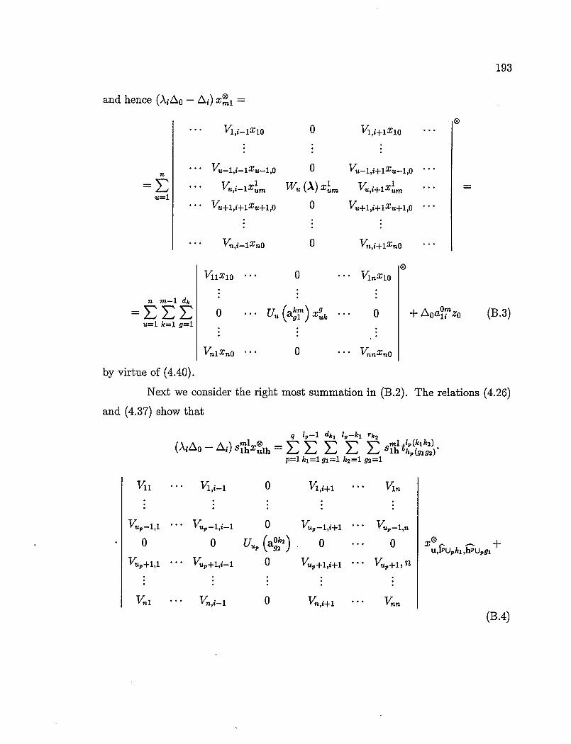
193
and hence (A 0 - z) x 1 =
t= l
n rn-i 4
=:: u=1 k=1 g=1
v1,i—ixio 0
V_i,_ix_i,o 0
V,i_iX Wu Zurn
V+i,+ix+i,o 0
vn,i—lxno
V11x10
0
0 V7x10
0 Uk 0
0 ... V0 xo
+ /0 OM a z0 (B.3)
by virtue of (4.40).
Next we consider the right most summation in (B.2). The relations (4.26)
and (4.37) show that
V11
MI 0 q i,i 4 l-ki rk2 mltlp(klk2)
OiAO - L) Sihxulh = E E > E E 81h hp(g192) p=1k1=lgi=1 k2=1 g21
v1,i.._1 0 Vi,+i •.. V1.
V,_1,1 V9_17 _1 0 VL,_i,fl
0 0 Uup (a 2) 0 •.. 0
vuP +i,i V+i,_i 0 V+i,+i vup+i,
vni Vn,i_i 0 V,1+i vnn
Xe - - + u,1PUkj ,hPug1
(B.4)

194
0 V1,+1
0 V, +1
yin
VlL _1,fl
0
(B.5)
Here we use the symbols i, Iii' and uI' to denote omission of the component with the index p in multiindices 1, h and u respectively. The symbols P U,, k1 and U,, g
indicate the replacement of the component 1, in 1 with k1 and the replacement of
the component h,, in li with g1 respectively. For 1 E m,q we write L = EL 1i and
Lp = The symbol L,, is well defined also for
For q = 2 the sum of terms (B.5) over u E 22, 1 E 'm,2 and h E xi equals
2
E .m(1112) EV1(h1h2)
UEQ2 lE'm,2 hEx1 P 1
V11 ... 0
O1\ 0 U (ah)
V 1 •.. 0 Vnn
Xø,
In the following calculation we use the relation (4.37) and the definitions of the sets
of multiindices. Note that EIE m2 = E J' E 12=11 = EI E 2. Then the above
expression is equal to
rn—i d,1
uEQ2 l=l hi=i
V11 ... 0
lim\ 0 •.. u 2 (ah1l) 0
Vni... 0
0 'tz ,11h1

lGWm,q WZX1 lEm-1,q-1 hPEX1
In the summation E1E m _I,q EL
that have L <k'. Thus
195
rn-i d12
+2>2E UE≤2 12=1 h2=i
V11 ... 0 •••V1,
12rn\ 0 •.. U", (a 21, 0
vni."
n n m-1 di
tL1i1L2.1,U2Ul 1=1 h=i
V11 ...
0 ... V nn
0
0 -
XU2 ,12h2 -
lrn\ 0 U 2 (ahi) 0
vni ... 0
Now we add the expressions (B.3) and the above one. The sum is
n rn-i d1
IL=1 l=i h=i
V11
V12
vni
Vi,i_i Ui (at) vi,i+i •.. V1 v2,1_i U2 (at) v2,+i •.. V2 n
vn,_i (IM a)
= E E 1oalm h1ix + /oa?rzo.
0
1=1 h=i
From the definition of the sets of multiindices it follows that
m-Lp d,
:= I-- -- l=i h,=i
a value k = k' appears exactly for those 1 E 'm—i,q
rn-i rn-i
(B.8) lE''m-i,q k=L k=q lE'k,q
Applying relation (B.7), Corollary 1.24, (i) and relation (B.8), respectively, it follows
that lk1 rk2
E rnl .l(k1k2) = 1En,qhEX1kii91i k2=1 92=1 Sih t h (gigs)
(B.9)

196
rn-L-1 dk1 m-L-ki rk2 m-L d1,,
= E l"E'i m i,q i IEX k1=1 gj=1 k2=i 92=1 1=ki+k2 h=i
lv
MI 1(/c,k2) - Sihth(9192) -
rn-L rk2 rn-k2 4 3 k31 .m(k2k3)
= E > S9 h 1 (9293) -
lEm-i,q hEX1 k2=i 921 k3=L 931
rn-i 4 3 rn-k3 rk2 k31 .rn(k2k3)
= E > s9 1(gg,) k3=P93=ilEk3,9 hEX1 k2=1 921
In the step (B.1O) of the above calculation we wrote l, instead of k1 and hp
of gi. Next we sum the terms (B.4) over 1 E 'm,q and h E X1. From the result of the
previous calculation it follows that the sum is equal to
rn-i dk3 rn-k3 r2 k31 .rn(k2k3)
S9 'i(gg)
k3=p931 iEk3q hEX1 k2 1 921
V11 ... 0 yin
U(a 2) ... 0
vni... 0
Xu ,l,h.
Here we write l, instead of k1 and 1i instead of g1 as in (B.10). Using the relation
(4.37) it follows that the above sum is equal to
rn-i dk3
k3=p931 iEk3,q hEX1
k31 S9 h
V11 ... 0 •••V1,
k3 0 0 u,, (a j) ...
Vnl ...
Xu ,l,h. (B.12)
Similarly to when we showed that (B.9) equals (B.11) we now show, using
Corollary 1.24 and relation (B.8), that for any index p E q (q ≥ 3),
m-1 4 3
Mi k31v -
ih = S- h P1(93hp) - lE q hEX1 lEm,q hEx1 k3L 93=1
rn-i 4 3 rn-k3 "lp
= k3 1P tm (3lp) -
k3=L 931 1p1 h=i S i(93h) -
l'E'vn_i,q_i hPEXj-

197
rn-i dk3 - k3 rip
= 8k31P > .m(k31,) g3 —h Vi(93h)
k3=q93r1 hl'EX1 1,,=l h,,=i
We use this equality to show that the sum over 1 E 1 ,,,,q and h E xi for q ≥ 3 of the terms (B.5) is equal to
rn-i dk3 k3 rip
E 1(g3h) k3=qg3=ij I1PEXr
rn-i dk3
V11 ... 0
0 u (ar") •.. 0
k31 = k3=q93=i IEk3,q-1 hEX1
V11 ... 0
k3rn\ 0 U (a3 )
uP,IP ,hP
Vnn
(B.13)
Next the sum of the expressions (B.13) over q = 3, 4,. . . , min {m, n} and u E fq is
min{m,n} rn-i 43 k31 E >
q=3 UE q k3=q931 lEk3,q...i hEX1
vu ... 0
k3 0 UtL (a) ... 0
Vni... 0 ...Vnn
= uP,1,h
min{rn,n}-i n rn—i 4 3
=
q=2 UE q v=i,vuk3=qg3i tEk3,q_1 hEx1

198
V11... 0
o •.. Uv(ak3m\ •.. 0 g31 ) 0 Xu1h.
Vni... 0
If we reverse the order of summation over q and k3 we have
min{m,n} rn—i rn—i min{k3,n} min{m,n}—i rn—i rn—i min{k3,n-1j
LL=LL and E E = E E q=2 k3=q k3=2 q=2 q=2 k3=q k3=2 q=2
(B.14)
From (13.12), (B.14) and the last relation it follows that the sum of terms (B.4) for
q ≥ 2 and terms (B.5) for q ≥ 3 over u E q, 1 E q,m and h E Xi is
rn—i 43 min{k3,n} q
EL L LLs k3=2g3=1 q=2 uEqP=ilEk3,q hEx1
rn—i dk3 min{k3,n-1j
V11 ... 0
0 •.. Up (ar) 0
vni ... 0
L ELEL k3=293=1 q=2 UEflq Vl,VUIEk3,q hEX1
V11 ... 0
0 U(a) •.. 0
Vni... 0
rn—i 43 min{k31n}
...Vnn
k31 S9 h
0 Xu1h -
=EE E LEE k3=2 93=1 q=2 UE≥qlEk3,qhEX1
V11 vi,_i Ui (ar) v1,+1 V1 V2,_1 U2 (ar) v2,+1
vi v,_i u (ar) v,1+1
k31 Sg3 h•
yin
V2
Vnn
0 Xu1h -
0 'u,1,h

199
rn—i dk3 min{k3,n} k3m 0
sIog3h a9311xlh. k3=2g3=1 q=2 lEk,q hEX1
(B.15)
Then it follows from the equality (B.2) and the calculations that followed it that
(Az0 - z is equal to the sum of the expressions (B.6) and (B.15), and thus
rn—i 4 rn—i dk min{k,n}
= I oaglix km + Loazo + > soagli4
k=i g=i k=2 g=i q=2 lEk,q hEX1
rn—i d1 (Xk mn{k,n} \ km g+ ghlhli ski x +zoazo=
k=1 g=i kq=2 l€cI k,q hExi
rn—i d1 = /0 km OM az + Aoa li
k=i g=1
0

200
Index
A decomposable tensor, 8
admissible set, 23 E
array
commutative, 9 eigenspace
reduced commutative, 12 of a commutative array, 10
arrays of a multiparameter system, 71
similar commutative, 9 eigenvalue
ascent completely derogatory, of a multi-
of an eigenvalue, 127 parameter system, 160
associated system nonderogatory, 14
of a multiparameter system, 62 nonderogatory of a multiparameter
system, 78
C nonderogatory, of a multiparameter
change of basis system, 70
admissible, 11 of a commutative array, 10
commutative array, 9 of a multiparameter system, 68
reduced, 12 semisimple, 130
commutative arrays, 9 simple, 31
similar, 9 simple of a multiparameter system,
cross-section 79
column, 9, 12 eigenvector, 71
row, 9, 12 of a commutative array, 10
D I
decomposability set, 63 invariant, 94

201
J determinantal, 61
Jordan chain induced, 8
of a matrix, 2
of a matrix polynomial, 118 pair of matrices
maximal, 120 equivalent, 92
K R Kronecker basis, 96
regularity conditions, 32 Kronecker canonical form, 93-94
representation by a multiparameter Kronecker chain, 96
system, 67 Kronecker product, 75
representation by tensor products, 51
M dimension, 53
matching conditions, 32 minimal dimension, 53
matrix root subspace
blockwise connected, 54 of a commutative array, 10
connected, 53 of a multiparameter system, 71
self-adjoint, 9 root vector, 71
symmetric, 9 for a commutative array, 10
multiparameter system, 60
diagonal, 60 scalar product, 8
elliptic, 132 on a tensor product space, 8
nonsingular, 62 set
right-definite, 130 decomposability, 63
self-adjoint, 129 set of invariants, 94
upper-triagonal, 60 of the kernel kerL, 104
weakly-elliptic, 131 a-shift of a Kronecker chain, 97
o spectrum
operator of a commutative array, 10
Lo-self-adjoint, 130 of a multiparameter system, 68

202
structure triple, 24
subspace
marked invariant, 106
symmetrization
of the array A°', 133
system
associated of a multiparameter sys-
tem, 62
multiparameter (see also multipa-
rameter system), 60
T
tensor
decomposable, 8
tensor product space, 8
transformation
induced linear, 8
U
upper Toeplitz form, 15


