Combining Markov Switching and Smooth Transition in Modeling Volatility: A Fuzzy Regime MEM

Combining Markov Switching and SmoothTransition in Modeling Volatility:

A Fuzzy Regime MEM

Giampiero M. GalloDipartimento di Statistica, Informatica, Applicazioni “G. Parenti”, Universita di Firenze

Via G. B. Morgagni, 59 - 50134 Firenze, Italy ([email protected])

Edoardo OtrantoDipartimento di Economia and CRENoS,

Universita di Messina, Piazza Pugliatti, 1 - 98122 Messina, Italy ([email protected])

Abstract

Volatility in financial markets alternates persistent turmoil and quiet periods.Modelling realized volatility time series requires a specification in which these sub-periods are adequately represented. Changes in regimes is a solution, but the questionof whether transition between periods is abrupt or smooth remains open. We providea new class of models with a set of parameters subject to abrupt changes in regimeand another set subject to smooth transition changes. These models capture the pos-sibility that regimes may overlap with one another (fuzzy). The empirical applicationis carried out on the volatility of four US indices.

Keywords: Volatility modeling, Volatility forecasting, Multiplicative Error Model,Markov Switching, Smooth Transition

1

1 IntroductionA recent strand of financial econometrics literature underlines as the profile of the realizedvolatility of financial time series is subject to frequent changes, which can assume theform of an abrupt change of regime, a smooth transition toward a different regime, anisolated jump, etc. Several recent studies develop models capturing all these features orconcentrating on just some of them. For example, Gallo and Otranto (2015) extend thefamily of Asymmetric Multiplicative Error Models (AMEM) of Engle (2002) and Engleand Gallo (2006) to include Markovian changes in regime (abrupt changes) and smoothtransitions to other regimes (gradual changes) with two separate models, called MarkovSwitching (MS)–AMEM and Smooth Transition (ST)– AMEM respectively. Andersenet al. (2007) provide the specification extensions related to jumps by inserting in the HARmodel of Corsi (2009) an explicative variable depending on the comparison between therealized volatility and the realized bi-power variation of the time series, whereas Caporinet al. (2014b) add, in the same HAR model, a volatility jump term following a compoundPoisson process. A similar extension was adopted by Caporin et al. (2014a) to includejumps in the MEM.

The correct detection of the several kinds of change is a crucial task in the analy-sis of the forecasting performance of the models. A typical result is the trade–off ex-isting between the in–sample and out–of–sample performance; in particular, Gallo andOtranto (2015), analyzing the realized kernel volatility (Barndorff-Nielsen et al., 2008)of the S&P500 index with several alternative models belonging to the AMEM and HARclasses, notice a better in–sample fitting of the MS–AMEM and a superior out–of–sampleperformance of the ST–AMEM. Of course, since they were obtained on just one series,the generalization of these results is one of the goals of this paper. Moreover, it is ap-pealing to seek for a model characterized by good performances in both the in–sampleand out–of–sample perspective, giving it an intermediate position between MS–AMEMand ST–AMEM. Our suggestion is to provide a new model which contains both kinds ofdynamics, the MS and the ST, involving the possibility to capture both the abrupt and thegradual changes in the series.

This idea is developed by considering the coefficients linked to the level of the volatil-ity subject to discrete changes (represented by different regimes or states) and the coeffi-cients representing the dependence on the past as continuously time–varying, by using asmooth transition function depending on a forcing variable known one period in advanceand related to the series analyzed. This specification provides a range of possible valuesof the local average volatility within each regime which may be overlapping, losing theclassical definition of regime linked to well separate states. This is consistent with therealistic cases in which some periods can not be cleared assigned to a certain regime.For this reason we define this class of models the Fuzzy Regime AMEM with n states(FR(n)–AMEM).1

We will verify the in–sample and out–of–sample performance of this new class ofmodels applying them to four different realized volatility series and comparing them with

1This model has some similarities with the Flexible MS model proposed by Otranto (2015), providingthe possibility to have time–varying coefficients within each regime, but not the possibility of overlappingstates.

2

the MS– and ST–AMEMs of Gallo and Otranto (2015) to verify if they are able to capturethe better in–sample characteristics of the first and the out–of–sample ones of the latter.Moreover, we will estimate also the classical AMEM and HAR as useful benchmarks.

The paper is organized as follows: in the next section we will describe the FR(n)–AMEM, with a particular focus on the simple 2-state case to illustrate the nature of thefuzzy regimes. Section 3 is devoted to the empirical application of the model. We first de-vote some special attention to the comparison of the information derived from the FR(2)model with those derived from MS(3) and ST models for the S&P500. We then extendthe number of models and the number of US realized kernel volatility time series includ-ing next to the S&P500, also the Russell 2000, the Dow Jones 30, and the Nasdaq 100.In– and out–of–sample performances are evaluated on the basis of single loss functionsand a synthesis thereof to evaluate contemporaneously the in–sample and out–of–sampleperformance. Some final remarks conclude the paper.

2 Combining Switching Regimes and Smooth TransitionsThe Multiplicative Error Model (MEM) has shown to have many desirable properties forthe analysis of the realized volatility. Among the reasons that enable its success we citethe direct representation of the levels of volatility without (log) transformations and thepossibility to extend it to include asymmetric effects (Engle and Gallo, 2006), Markovianor smooth transition dynamics (Gallo and Otranto, 2015), presence of jumps (Caporinet al., 2014b). The model we propose is a combination of the MS–AMEM and the ST–AMEM proposed by Gallo and Otranto (2015).

Let yt the realized volatility of a certain index at time t (t = 1, . . . , T ), µt,st a latentfactor representing its conditional mean, st a discrete latent variable ranging in [1, . . . , n],representing the regime at time t, εt a random disturbance and Dt a dummy variablewhich is 1 when the return of the index at time t is negative. The MS(n)–AMEM, wheren indicates the number of regimes, is given by:

yt = µt,stεt, εt|st ∼ Gamma(ast , 1/ast) for each t,

µt,st = ω +∑n

i=1 kiIst + αstyt−1 + βstµt−1,st−1 + γstDt−1yt−1

(2.1)

The first equation follows the typical MEM structure suggested by Engle (2002), obtainedas the product of two positive unobservable factors; as in Engle and Gallo (2006), theGamma distribution of the disturbances depends only on the scale parameter, which in(2.1) changes with the regime (ast), so that its mean is equal to 1 and its variance equal to1/ast . The second equation represents the dynamics of the mean, which follows a sort ofGARCH(1,1)–type dynamics, with the intercept ω+

∑ni=1 kiIst (where Ist is the indicator

of the state; k1 = 0, ki >= 0 for i > 1), which increases with the state st. The dynamicsof the latent state variable st is driven by a Markov chain, such that:

Pr(st = j|st−1 = i, st−2, . . . ) = Pr(st = j|st−1 = i) = pij. (2.2)

We hypothesize that the volatility levels increase with the regime st.

3

Gallo and Otranto (2015) define also the ST–AMEM as:

yt = µtεt, εt ∼ Gamma(a, 1/a) for each t

µt = ω + αtyt−1 + βtµt−1 + γtDt−1yt−1

(2.3)

The coefficients αt, βt, γt are smooth transition parameters,2 which follow a simple lineardynamics depending on a smooth function 0 ≤ gt ≤ 1:

αt = α0 + α1gtβt = β0 − β1gtγt = γ0 + γ1gtgt = (1 + exp(−δ(xt − c)))−1.

(2.4)

where xt is a forcing variable driving the smooth movements, generally linked to thevolatility movements. Imposing the nonnegativity of the coefficients α0, α1, β0, β1, γ0,γ1, the effect on the time-varying coefficients αt, βt, γt, increasing the smooth functiongt, is an increase of the coefficients αt and γt, expressing the effect of the last volatilitylevel, and a decrease of βt, which, in turn, contributes to a decrease in the persistenceeffect. Notice that in (2.3) the coefficient a of the Gamma distribution is not time–varyingbecause the levels of the volatility are assumed not subject to discrete jumps, but to con-tinuous changes; in practice the smooth transition changes of the level of volatility capturealso the possible different spread and the model can fit the data with a constant variance.

The FR(n)–AMEM combines the characteristics of models (2.1) and (2.3) and it isdefined as:

yt = µt,stεt, εt|st ∼ Gamma(a, 1/a) for each t,

µt,st = ω +∑n

i=1 kiIst + αtyt−1 + βtµt−1,st−1 + γtDt−1yt−1

(2.5)

As in the ST–AMEM, the Gamma distribution of the disturbances depends only on theconstant parameter a, whereas the second equation represents the new specification of thedynamics of the mean, which is composed by one switching and three smooth transitioncoefficients. The switching coefficient is the intercept and the coefficients αt, βt, γt aresmooth transition parameters, following the (2.4) specification. In our applications wewill consider the lagged VIX (Whaley, 1993) as forcing variable, but other choices arepossible.

Models MS(n)–AMEM and ST–AMEM are not nested in model (2.5). In fact for theMS–AMEM we hypothesize that αt = αst , βt = βst , γt = γst , which do not depend on gt,so that c and δ are nuisance parameters. The ST–AMEM is not nested in the FR–AMEMbecause it considers a constant intercept or an intercept depending on gt. When all thecoefficients are constant we obtain the simple AMEM of Engle and Gallo (2006).

The peculiarity of the FR(n)–AMEM is that the n regimes cannot be clearly separated,but the same observation could be assigned to a regime or another one, depending on thevalue of the smooth transition function gt. To better understand this characteristic, let

2In Gallo and Otranto (2015) γt was constant.

4

us consider the local average volatility (LAV hereafter) of the series yt, conditional onthe regime and the value of gt, under the usual stationarity hypothesis; this indicatorcorresponds to the unconditional volatility when all the coefficients are constant (as in theAMEM case). For the sake of simplicity let us consider the 2-state case, but the results areeasily extended to the general n-state model. Let ut,st,gt = E(µst,t|st, st−1, gt) the LAV attime t; it is derived from the second equation of (2.5) and is given by:

ut,st,gt = ω + k2I2 + (αt + βt + γt/2)ut−1,st−1,gt−1 (2.6)

Adding the constraint (α1 + γ1/2) ≥ β1, ut,st,gt will not decrease when gt increasesand will not decrease with the regime (ut,2,gt ≥ ut,1,gt because k2 ≥ 0). Also, whenst = st−1 and gt = gt−1, equation (2.6) can be written in a manner similar to the classicalunconditional volatility expression:

ut,st,gt =ω + k2I2

1− αt − βt − γt/2(2.7)

This implies that the minimum (maximum) of ut,st,gt is reached in correspondence ofboth gt and gt−1 equal to 0 (1). As a consequence, we can detect a global minimum andmaximum of the LAV and its range for each regime; calling ulst and uhst the lower andhigher extremes of the LAV in regime st, we have:

ul1 = min(ut,1,gt) = E(µt|st = 1, st−1 = 1, gt = 0) = ω1−α0−β0−γ0/2

uh2 = max(ut,2,gt) = E(µt|st = 2, st−1 = 2, gt = 1) = ω+k21−α0−α1−β0+β1−(γ0+γ1)/2

uh1 = max(ut,1,gt) = E(µt|st = 1, st−1 = 2, gt = 1) = ω + (α0 + α1 + β0 − β1 + γ0+γ12

)uh2

ul2 = min(ut,2,gt) = E(µt|st = 2, st−1 = 1, gt = 0) = ω + k2 + (α0 + β0 + γ02

)ul1(2.8)

The two ranges of the local average volatilities in different regimes may overlap, provid-ing a sort of fuzzy regime. In practice model (2.5) provides an inference on the regime aseach MS model, but the levels of the LAV are not clearly separated among regimes. Inother words, if uh1 > ul2, then the set [ul2;u

h1 ] is the overlapping area and the local average

volatilities can be classified (borrowing the set theory terminology, see Zadeh (1965)) inthe following way:

• crisp zone 1: local average volatilities ranging in [ul1;ul2];

• fuzzy zone: local average volatilities ranging in [ul2;uh1 ];

• crisp zone 2: local average volatilities ranging in [uh1 ;uh2 ];

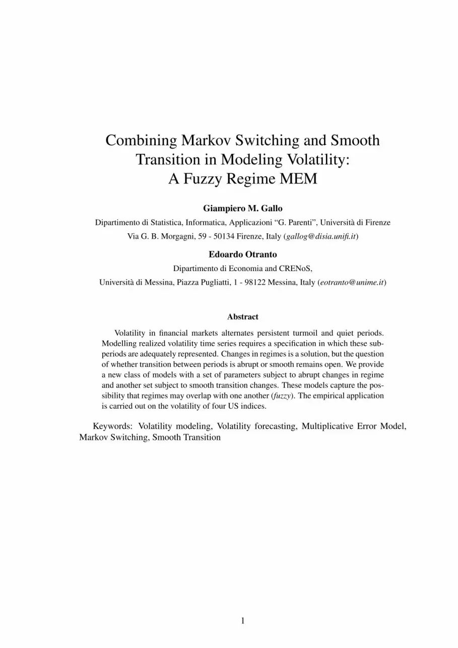
In Figure 1 we illustrate a graphical example to better interpret the fuzzy and crispzones; we consider a simple FR(2)–AMEM with βt = γt = 0); the other coefficients areω = 1, k2 = 3, α0 = 0.5, α1 = 0.4. The Figure shows the behavior of the LAV in the tworegimes in correspondence of gt. The two curves do not intersect but, in the fuzzy zone(gray area), they can assume the same value in correspondence of two different values of

5

gt; in other words a certain level of the unconditional volatility can be reached in state 1in correspondence of a certain gt or in state 2 in correspondence of a lower gt. In practicein the fuzzy zone the assignment of an observation to regime 1 or 2 depends on the valueof gt.

The extension to the n−state case is simple; for the state j, the range of the LAV isgiven by:

ulj = ω +∑j

i=1 ki + (α0 + β0 + γ0/2)ul1

uhj = ω +∑j

i=1 ki + (α0 + α1 + β0 − β1 + γ0/2 + γ1/2)uhn

(2.9)

From (2.9), it is evident that the differences between the lowest (highest) LAV of twostates is due exclusively to the changes in the intercept, so it is likely that the fuzzy zonesare very large with respect to the crisp zones. This fact could imply some difficulty inthe interpretation of regimes when the number of states is more than two, since severalregimes will have overlapping areas. What we want to stress is that we gain in termsof flexibility of the model and goodness of fit, as empirically shown in what followsespecially by the FR(3)–AMEM. Nonetheless, we can discuss some features of the FR(2)–AMEM model to provide some graphical illustration of the mechanisms behind this newapproach.

For reference purposes, let us introduce a corresponding formula for the MS–AMEM,given by:

ut,st = ω +∑n

i=1 kiIst + (αst + βst + γst/2)ut−1,st−1 if st 6= st−1

ut,st =ω+

∑ni=1 kiIst

1−αst−βst−γst/2if st = st−1

(2.10)

whereas the one for the ST–AMEM is:

ut,gt = ω + (αt + βt + γt/2)ut−1,gt−1 (2.11)

We can use the strong relationship between the regime and gt to assign the observa-tions to a crisp or a fuzzy zone. Let us consider again the two-state case (the extensionto a generic n−state case is trivial but notationally cumbersome); the conditional mean(second equation of (2.5) is:

µst,t = ω+k2I(st)+α0yt−1+β0µst−1,t−1+γ0Dt−1yt−1+gt(α1yt−1−β1µst−1,t−1+γ1Dt−1yt−1)

If the observation at time t falls in a fuzzy zone, then there will exist a value of gt (call itg∗t ) such that:

g∗t =µst,t − ω − k2(1− Ist)− α0yt−1 − β0µst−1,t−1 − γ0Dt−1yt−1

α1yt−1 − β1µst−1,t−1 + γ1Dt−1yt−1

and 0 ≤ g∗t ≤ 1.If g∗t < 0 or g∗t > 1, it is a not admissible value and the observation at time t falls in a

crisp zone.

6

3 Empirical Analysis

3.1 The Data and the ModelsWe apply the FR(n)–AMEM, with n = 2 and 3, to four realized kernel volatility seriesof the main indices of the US markets: S&P500, Russell 2000, Dow Jones 30, Nasdaq100. The forcing variable adopted for the smooth transition function is the lagged VIX.The realized kernel volatility is an estimator of the integrated volatility of a diffusion pro-cess, proposed by Barndorff-Nielsen et al. (2008), possessing the important property ofrobustness to market microstructure noise. The data relative to the series analyzed in thiswork are taken from the Oxford-Man Institute Realized Library version 0.2 (Heber et al.,2009), and are annualized, i.e. we consider the square root of the realized kernel variancemultiplied by 100

√252. We cover the period 2 January 2004–5 May 2015 with daily

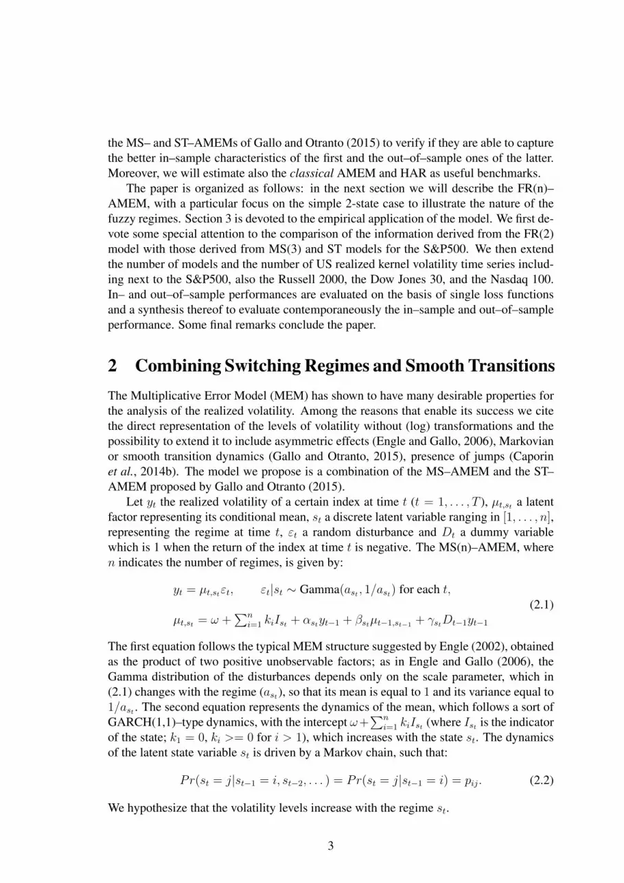
observations, using the data until 31 December 2013 for the in–sample evaluation andthe rest for the out–of–sample case. In Figure 2 the four series are depicted. They showsimilar behavior with common highest peaks, in particular the bursts of volatility startingin September 2008. The out–of–sample period is characterized by frequent movementswith no high peaks.

In addition to the FR(2)–AMEM and the FR(3)–AMEM we have estimated a MS(3)–AMEM and a ST–AMEM, following the specification given in Gallo and Otranto (2015).Moreover, we have considered two simple benchmark models as AMEM and HAR:

• AMEM:yt = µtεt, εt ∼ Gamma(a, 1/a) for each t,

µt = ω + αyt−1 + βµt−1 + γDt−1yt−1,

• HAR:yt = µtεt, εt ∼ Gamma(a, 1/a) for each t

µt = ω + αDyt−1 + αW y(5)t−1 + αM y

(22)t−1 ,

where the three independent variables of the second equation express past volatili-ties aggregated at daily, weekly and monthly frequency respectively.

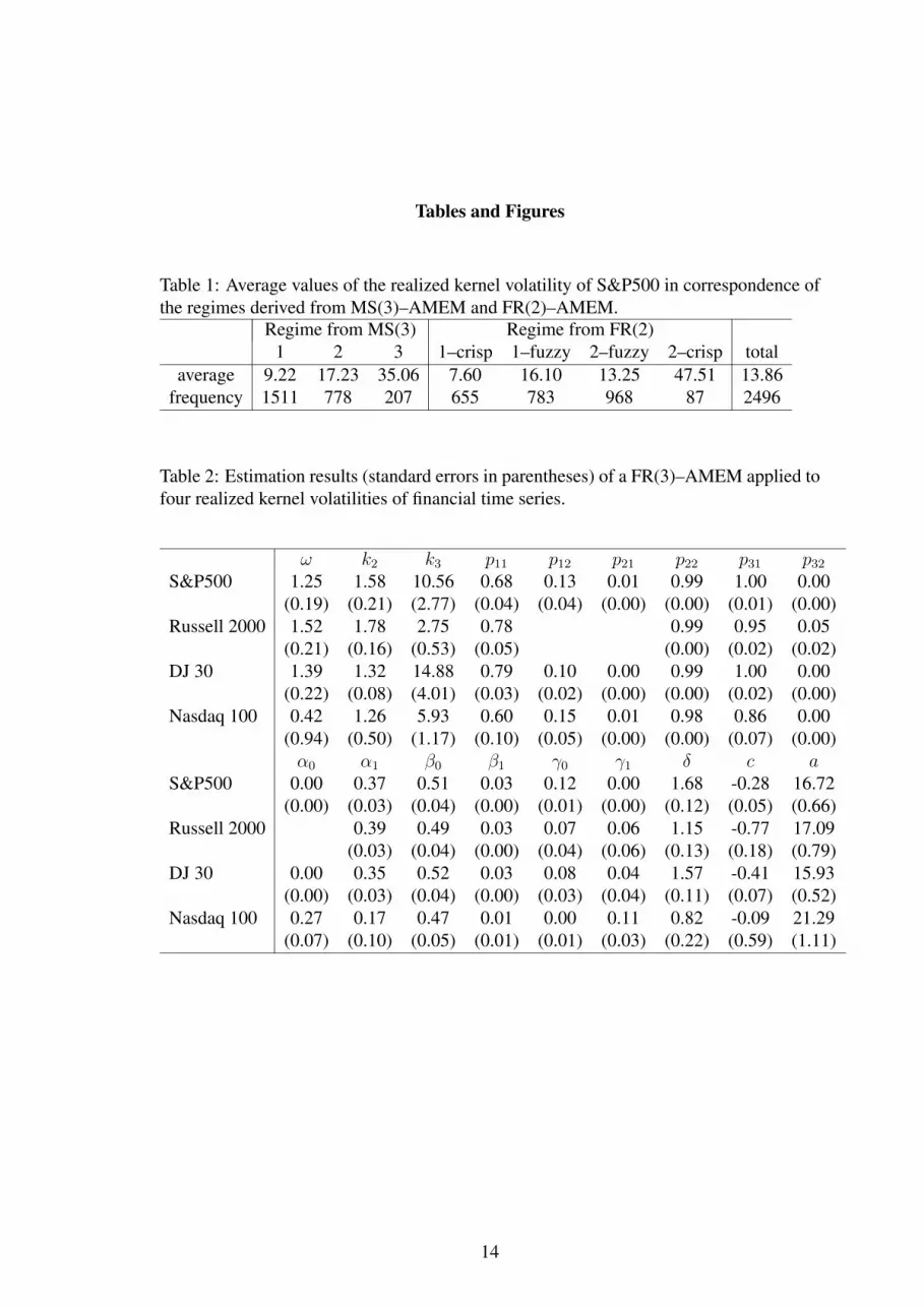
In Table 2 we show the estimation results for the four indices using the FR(3)–AMEM,that, as we will see, shows in general the best performance. All the indices are charac-terized from a strong persistence in state 2 and the probability to switch to state 1 at timet, when st−1 = 3, near to 1. For the Russell index we set the parameters p12, p21 and α0

equal to zero to get convergence.In Table 3 we show the extreme values of the LAV for the ST, FR(2) and FR(3) models

and the LAV of each state of MS(3) (expressed by the second equation in (2.10), which isthe most frequent case, as showed in the first panel of Figure 3). It is interesting to noticeas the highest values of the ST–AMEM are very low if compared to the highest peaks ofthe realized volatility. Also the presence of a third regime in the FR model provides thepossibility to identify very high peaks, excluding the Russell case, where the maximumvalue of the LAV in the third regime is equal to the LAV of the third regime of the static

7

MS(3) model. Of course these extreme values are theoretical, depending, in practice, onthe value of gt in the sample adopted.

3.2 Interpretation of Fuzzy RegimesIn order to gain deeper insights on the features of the FR–AMEM (in particular for theinterpretation of the regimes), contrasting its results with those derived from a suitableMS–AMEM and a ST–AMEM. For the sake of illustration, we keep on considering a2-state FR model, with two crisp and one fuzzy zone; the natural comparison is madein terms of a 3-state MS model, because the fuzzy zone of a FR(2)–AMEM could beconsidered as an alternative to the second regime of a MS(3)–AMEM. In what follows,the inference on the Markovian regimes is obtained from the smoothed probabilities ineach model, calculated over the full span, assigning the time t to the regime with thehighest smoothed probability at that time.

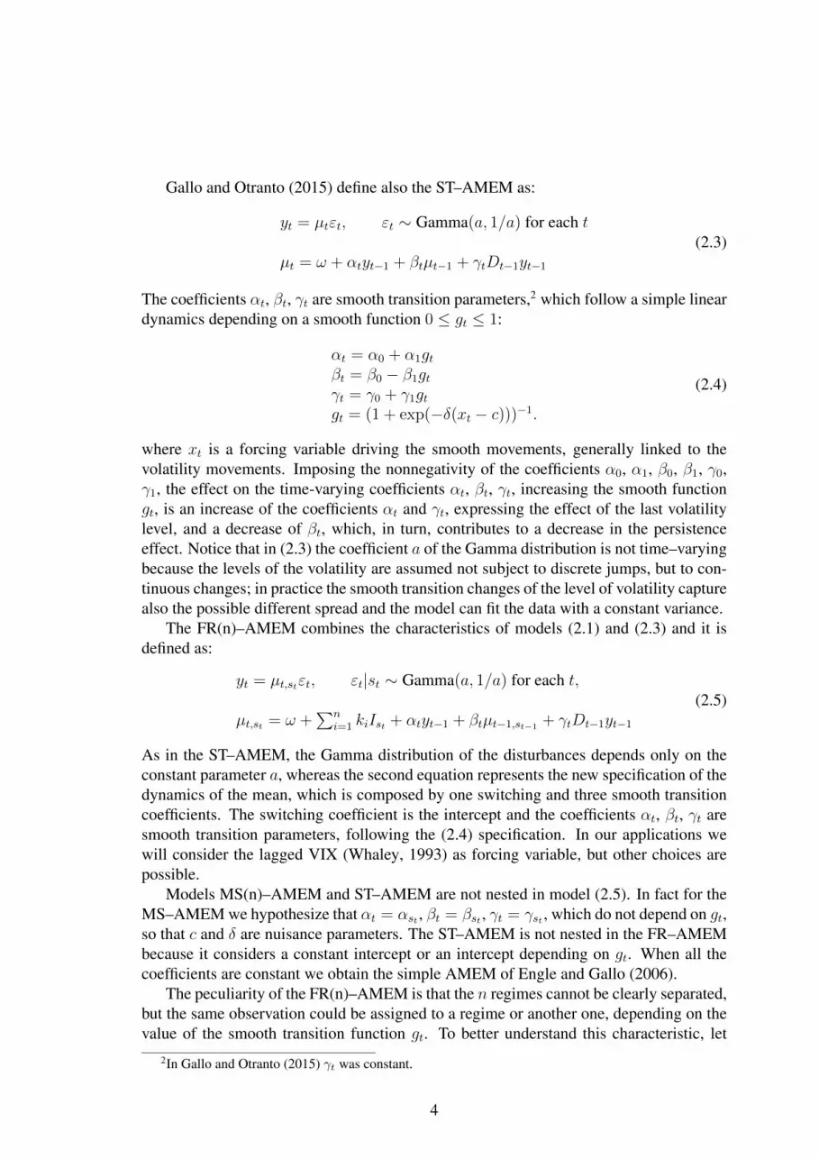
In Figure 3 we show the time series profile of the local average volatilities derived forthe three models, starting from the MS(3)–AMEM (expression (2.10) in the top panel),then the ST–AMEM (expression (2.11) in the middle panel) and then the FR(2)–AMEM(expression (2.6 in the bottom panel). In all three panels we overlap the values of thelocal average volatilities to the realized volatility series. For all models, we confirm thedifficulty highlighted by Gallo and Otranto (2015) to capture the burst of volatility ofOctober 2008. For the MS(3)–AMEM, it is clear that its LAV is subject to abrupt anddiscrete changes, (usually between three constant levels): while, on the one hand, thisallows for a clear identification of which regime each observation is attributed to, on theother, it presents the inconvenient feature that fairly different values of realized volatilityare associated with the same level of LAV. This is apparent from the first period in whichwe have a prolonged constant level of LAV, but it is even more striking for the thirdregime, where the LAV is often very high relative to the corresponding observed volatilityvalue. The ST–AMEM and FR(2)–AMEM show a similar dynamics of local averagevolatilities relative to one another, but the latter better follows the profile of the realizedvolatility, especially for its highest values (the maximum level of the LAV in the STmodel is equal to 32.3 points versus a maximum of 41.7 in the FR case). In practice,the FR model has the same desirable features as the ST model in terms of flexibility, butexploits the MS properties to better identify the frequent jumps and abrupt changes.

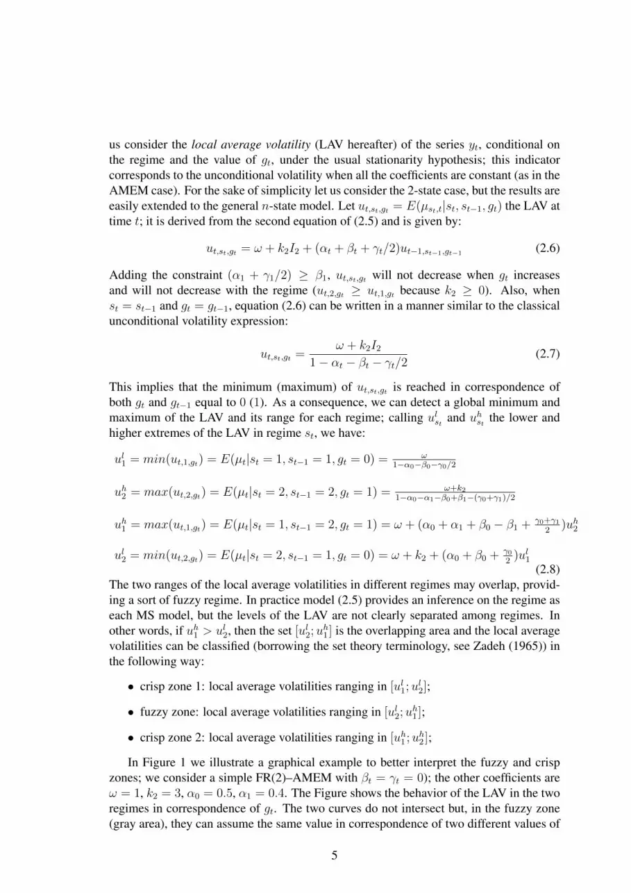
In Figure 4 we reconstruct the distributions of the realized kernel volatilities for theMS and the FR models, highlighting the regimes identified on the basis of the inferenceon the states. The different attribution of observations to regimes across models is moreevident for lower values, while the highest values are uniformly assigned to the highestregime. In reference to the characterization of fuzzy regimes, we can notice that theyare typical for volatility values under 40%. Looking at Table 1, the average value of thevolatility when the observation falls in regime 2, but in a fuzzy zone, is lower than theaverage of the fuzzy zone in regime 1; this result is coherent with Figure 1, where we sawthat the grey area is common to the lowest values of regime 2 and the highest values ofregime 1. From the same table, let us notice that the regime 2–crisp within the FR modelcaptures just the highest peaks: on average, this regime includes fewer observations andhas a higher average value (by more than 12%) than the third regime within the MS model.

8

By and large, the regime 2–fuzzy in the FR model matches the highest peaks of regime1 in the MS(3) model, whereas observations in the regime 1–fuzzy fall into the secondregime of MS(3). This regularity is confirmed by comparing Figure 5, where we showthe inference about the regimes within the FR(2) model, with the first graph of Figure 3,where derive the inference about the regimes within the MS(3) model.

In Figure 5 we distinguish between fuzzy (dotted blue) and crisp (black continuous)classification within either regime. Notice that the volatility values belonging to theregime 1–crisp are very small, isolating the periods of very low volatility, whereas theregime 2–crisp corresponds only to the highest episodes. The observations in the fuzzyarea are obviously in–between cases: we can notice that the regime 1–fuzzy generallycaptures cases in which there is a smooth reduction in volatility whereas regime 2–fuzzygenerally corresponds to a smooth increase in volatility. Typically we reach regime 2–crisp by passing through regime 2–fuzzy (a burst from a volatility already increasing),while the downward evolution from regime 2–crisp is characterized by a change to regime1 entering its fuzzy zone. For ease of reference, we report in Table 4 the reconstruction ofturbulences occurring in the US and European markets which characterize the dates as-signed to regime 2–crisp. Reassuringly, we find all major related events, from Bear Sterns,to Lehman Brothers to the US Budget crisis and the evolution of the Greek debt crisis withthe inception of uncertainty about the solidity of the Euro institutional arrangements.

3.3 Comments on Other Models and Other IndicesThe inference on the regime is quite similar across the four indices. In Table 5 we showa classification of the dates, indicating the percentage of cases where a) the volatilitiesof the four indices at time t are all assigned to the same state, b) just three indices to thesame state, c) two indices to the same state and two to another one (but the same), d) twoindices to one state and the other two to two other separate states,3 using FR(3)–AMEM,FR(2)–AMEM and MS(3)–AMEM. For a large part of the observations we assign threeor four indices contemporaneously to the same state (cases a) and b)): in particular, morethan 88% using the MS(3)–AMEM, more than 81% using FR(2)–AMEM and more than94% using FR(3)–AMEM. The latter shows more than 61% of agreement of the indiceswithin the same regime (case a)).

The comparison among the six models (HAR, AMEM, ST–AMEM, MS(3)–AMEM,FR(2)–AMEM, FR(3)–AMEM) is conducted in terms of residual autocorrelation andMean Squared Errors (MSE) and Mean Absolute Errors (MAE) both for the in–sampleand out–of–sample cases. In Table 6 we show the p-values of the Ljung–Box statisticsfor each model and each index in correspondence of several lags. It is evident the pres-ence of residual correlation in the HAR model (a result coherent with (Gallo and Otranto,2015)), whereas the MEM family seems able to satisfy the hypothesis of uncorrelated-ness, with some exceptions. In particular we notice a disappointing performance of theMS(3)–AMEM for the Russell 2000 and a general improvement of the test statistics forthe FR model passing from 2 to 3 regimes.

We find interesting the models performance in terms of fitting and forecasting. As

3In the FR(2)–AMEM, the last case is not possible.

9

in Gallo and Otranto (2015), we have considered 1 and 10 steps ahead out–of–sampleforecasts, evaluating 336 observations corresponding to the most recent period (2014 andsome of 2015). For the out–of–sample forecasts we have used the model estimated in–sample, fixing the estimated parameters for the full out–of–sample period. In Table 7we show the loss functions for each index: in general, we confirm the result that theMS(3)–AMEM performs better than ST–AMEM in–sample and the opposite is true out–of–sample. One interesting feature of the FR models is their nature of striking a compro-mise between the two, as they reach a satisfactory performance across in– and out–of–sample, since they are almost always the best or the second best model.

To decide what model performs globally better in in– and out–of–sample terms, it isconvenient to evaluate the indices in relative terms, considering their relative performancewith respect to the HAR model adopted as a benchmark model. Each relative variation ofthe loss function l of model M is given by:

vM =lM − lHARlHAR

,

with generally an expected negative sign (an improvement relative to HAR). To synthesizeresults, a global loss function GM for model M may be derived as weighted average ofthe resulting six loss functions (MSE and MAE, in– and 1– and 10–steps ahead out–of–sample):

GM =∑l

wlvM ,∑l

wl = 1 (3.1)

We consider four possible global loss functions, differing by the set of weights used. Wechoose

1. uniform: each wl equal to 1/6;

2. oos oriented: the weights of the in–sample loss functions equal to 0.1 and theweights of the out–of–sample loss functions equal to 0.2;

3. oos short term (st) oriented: the weights of the 1–step ahead out–of–sample lossfunctions equal to 0.3 and the others equal to 0.1;

4. oos long term (lt) oriented: the weights of the 10–step ahead out–of–sample lossfunctions equal to 0.3 and the others equal to 0.1.

The performance in terms of global functions is better, the moreGM decreases away fromthe value GM = 0 (which marks the same performance as the HAR model).

In Table 8 we show the evaluation derived from the four alternative global loss func-tions (3.1). For the S&P500 index we notice a better behavior of the FR models consider-ing the uniform loss function; when the out–of–sample performance has more importancein the evaluation, the good behavior of the ST–AMEM predominates, but FR(2)–AMEMwins in the short term horizon; also FR(3)–AMEM is always the second best (the best inthe uniform case). For the Russell index the MS(3)–AMEM seems to have the best per-formance, but, recalling the results in Table 6, it suffers from a clear presence of autocor-relation in its residuals; again FR(3)–AMEM is always the second best and outperforms

10

MS(3)–AMEM in the short term forecasting. The DJ and Nasdaq indices clearly favorthe FR(3)–AMEM, which is the best model with respect to all the global loss functions,excluding the long term forecasting case of DJ, where it closely loses to ST–AMEM (witha difference, which is less than 0.002).

4 ConclusionsThe existence of waves of turbulence ensuing from events affecting the national and globaleconomies, has characterized the behavior of volatility in financial markets, posing a se-rious challenge to econometric modeling of the corresponding time series. The mainfeature that one can notice in the corresponding graphs is that the average level of volatil-ity changes through time at low frequencies, with short term dynamics around such levelsmarked by slow mean reversion (persistence).

In this paper, we have elaborated on a large stream of literature that extends the studyof volatility in a GARCH framework, by introducing Markov switching features to thespecification for the return conditional variance and, alternatively, Smooth Transitionacross different average levels; see, for example, Maheu and McCurdy (2002), Maheuand McCurdy (2007), Maheu and McCurdy (2011), McAleer and Medeiros (2008). Inparticular we have concentrated on Multiplicative Error Models and their MS and STextensions studied by Gallo and Otranto (2015) by introducing a new class of modelsthat combines features of both. The specification allows for a characterization of theobservations in which while maintaining assignment to regimes, within each regime weidentify observations belonging to a sharp characterization of the regime (called crisp)and observations assigned to another range, called fuzzy, seen as a sort of intermediatecase between regimes. From the empirical results, and for the case of two regimes, weinterpret the regime 1–crisp as a regime of low volatility, the regime 2–crisp as a regimecorresponding to major turmoil events. The fuzzy regimes are characterized by a slowincrease in volatility (and hence a slow transition from low to high volatility, regime 1–fuzzy), respectively, by a slow decrease in volatility (and hence a slow transition fromhigh to low volatility, regime 2–fuzzy).

The analysis was carried out on four major US indices which represent various degreesof market depth, capitalization and liquidity: we chose to specify models for the realizedkernel volatility measures which can be seen as the best available realized measures ofvolatility (with robustness to jumps and market microstructure noise). We had severalvariants of the suggested models estimated, changing the number of regimes consideredin the MS component, and keeping the Corsi (2009) HAR as a benchmark reference asin other studies. The estimation results were evaluated both in– and out–of–sample witha number of loss functions, then conveniently summarized in relative terms with respectto the benchmark and then aggregated in a global loss function with alternative choicesof weights to adhere to different goals a model could be geared to. The general result isthat the introduction of the fuzzy area allows for a convenient tradeoff between in–sampleperformance where MS models perform the best and out–of–sample, where the ST modelcomes out first, in line with Hansen and Timmerman (2015).

The fuzzy regime models also seem to capture the explosion in volatility following the

11

bankruptcy of Lehman Brothers in Sep.–Oct. 2008, in the two regime case, we are capableof interpreting each observation assigned to the regime 2–crisp in terms of major eventswhich affected the US markets with the evolution of the subprime mortgage crisis in2008 and then the US Budget and the uncertainty surrounding the Euro Area institutionalarrangements in 2011.

ReferencesAndersen, T. G., Bollerslev, T., and Diebold, F. X. (2007). Roughing it up: Including

jump components in the measurement, modeling and forecasting of return volatility.Review of Economics and Statistics, 89, 701–720.

Barndorff-Nielsen, O. E., Hansen, P. R., Lunde, A., and Shephard, N. (2008). Designingrealised kernels to measure the ex-post variation of equity prices in the presence ofnoise. Econometrica, 76, 1481–1536.

Caporin, M., Rossi, E., and Santucci De Magistris, P. (2014a). Chasing volatility: apersistent multiplicative error model with jumps. Technical report.

Caporin, M., Rossi, E., and Santucci De Magistris, P. (2014b). Volatility jumps and theireconomic determinants. Journal of Financial Econometrics, forthcoming.

Corsi, F. (2009). A simple approximate long-memory model of realized volatility. Journalof Financial Econometrics, 7, 174–196.

Engle, R. F. (2002). New frontiers for ARCH models. Journal of Applied Econometrics,17, 425–446.

Engle, R. F. and Gallo, G. M. (2006). A multiple indicators model for volatility usingintra-daily data. Journal of Econometrics, 131, 3–27.

Gallo, G. M. and Otranto, E. (2015). Forecasting realized volatility with changing averagevolatility levels. International Journal of Forecasting, 31, 620–634.

Hansen, P. R. and Timmerman, A. (2015). Discussion of “comparing predictive accuracy,twenty years later” by francis x. diebold. Journal of Business and Economic Statistics,33, 17–21.

Heber, G., Lunde, A., Shephard, N., and Sheppard, K. (2009). Omi’s realised library,version 0.1. Technical report, Oxford-Man Institute, University of Oxford.

Maheu, J. M. and McCurdy, T. H. (2002). Nonlinear features of realized fx volatility.Review of Economics and Statistics, 84(4), 668–681.

Maheu, J. M. and McCurdy, T. H. (2007). Components of market risk and return. Journalof Financial Econometrics, 5(4), 560–590.

Maheu, J. M. and McCurdy, T. H. (2011). Do high-frequency measures of volatilityimprove forecasts of return distributions? Journal of Econometrics, 160, 69–76.

12

McAleer, M. and Medeiros, M. (2008). A multiple regime smooth transition heteroge-neous autoregressive model for long memory and asymmetries. Journal of Economet-rics, 147, 104–119.

Otranto, E. (2015). Adding flexibility to markov switching models. Technical report,CRENoS Working Paper 2015/09.

Whaley, R. E. (1993). Derivatives on market volatility: Hedging tools long overdue.Journal of Derivatives, 1, 71–84.

Zadeh, L. (1965). Fuzzy sets. Information and Control, 8, 338–353.

13

Tables and Figures

Table 1: Average values of the realized kernel volatility of S&P500 in correspondence ofthe regimes derived from MS(3)–AMEM and FR(2)–AMEM.

Regime from MS(3) Regime from FR(2)1 2 3 1–crisp 1–fuzzy 2–fuzzy 2–crisp total

average 9.22 17.23 35.06 7.60 16.10 13.25 47.51 13.86frequency 1511 778 207 655 783 968 87 2496

Table 2: Estimation results (standard errors in parentheses) of a FR(3)–AMEM applied tofour realized kernel volatilities of financial time series.

ω k2 k3 p11 p12 p21 p22 p31 p32S&P500 1.25 1.58 10.56 0.68 0.13 0.01 0.99 1.00 0.00

(0.19) (0.21) (2.77) (0.04) (0.04) (0.00) (0.00) (0.01) (0.00)Russell 2000 1.52 1.78 2.75 0.78 0.99 0.95 0.05

(0.21) (0.16) (0.53) (0.05) (0.00) (0.02) (0.02)DJ 30 1.39 1.32 14.88 0.79 0.10 0.00 0.99 1.00 0.00

(0.22) (0.08) (4.01) (0.03) (0.02) (0.00) (0.00) (0.02) (0.00)Nasdaq 100 0.42 1.26 5.93 0.60 0.15 0.01 0.98 0.86 0.00

(0.94) (0.50) (1.17) (0.10) (0.05) (0.00) (0.00) (0.07) (0.00)α0 α1 β0 β1 γ0 γ1 δ c a

S&P500 0.00 0.37 0.51 0.03 0.12 0.00 1.68 -0.28 16.72(0.00) (0.03) (0.04) (0.00) (0.01) (0.00) (0.12) (0.05) (0.66)

Russell 2000 0.39 0.49 0.03 0.07 0.06 1.15 -0.77 17.09(0.03) (0.04) (0.00) (0.04) (0.06) (0.13) (0.18) (0.79)

DJ 30 0.00 0.35 0.52 0.03 0.08 0.04 1.57 -0.41 15.93(0.00) (0.03) (0.04) (0.00) (0.03) (0.04) (0.11) (0.07) (0.52)

Nasdaq 100 0.27 0.17 0.47 0.01 0.00 0.11 0.82 -0.09 21.29(0.07) (0.10) (0.05) (0.01) (0.01) (0.03) (0.22) (0.59) (1.11)

14

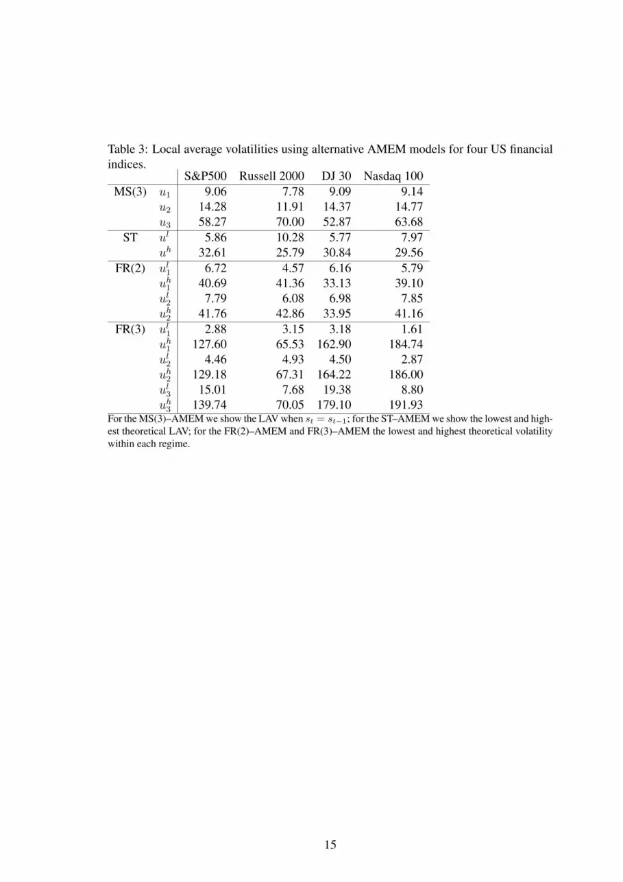
Table 3: Local average volatilities using alternative AMEM models for four US financialindices.

S&P500 Russell 2000 DJ 30 Nasdaq 100MS(3) u1 9.06 7.78 9.09 9.14

u2 14.28 11.91 14.37 14.77u3 58.27 70.00 52.87 63.68

ST ul 5.86 10.28 5.77 7.97uh 32.61 25.79 30.84 29.56

FR(2) ul1 6.72 4.57 6.16 5.79uh1 40.69 41.36 33.13 39.10ul2 7.79 6.08 6.98 7.85uh2 41.76 42.86 33.95 41.16

FR(3) ul1 2.88 3.15 3.18 1.61uh1 127.60 65.53 162.90 184.74ul2 4.46 4.93 4.50 2.87uh2 129.18 67.31 164.22 186.00ul3 15.01 7.68 19.38 8.80uh3 139.74 70.05 179.10 191.93

For the MS(3)–AMEM we show the LAV when st = st−1; for the ST–AMEM we show the lowest and high-est theoretical LAV; for the FR(2)–AMEM and FR(3)–AMEM the lowest and highest theoretical volatilitywithin each regime.

15

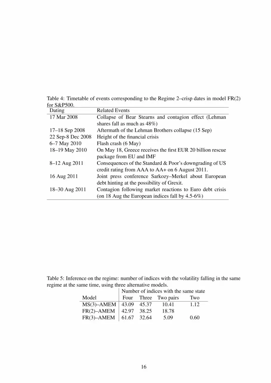
Table 4: Timetable of events corresponding to the Regime 2–crisp dates in model FR(2)for S&P500.Dating Related Events17 Mar 2008 Collapse of Bear Stearns and contagion effect (Lehman

shares fall as much as 48%)17–18 Sep 2008 Aftermath of the Lehman Brothers collapse (15 Sep)22 Sep-8 Dec 2008 Height of the financial crisis6–7 May 2010 Flash crash (6 May)18–19 May 2010 On May 18, Greece receives the first EUR 20 billion rescue

package from EU and IMF8–12 Aug 2011 Consequences of the Standard & Poor’s downgrading of US

credit rating from AAA to AA+ on 6 August 2011.16 Aug 2011 Joint press conference Sarkozy–Merkel about European

debt hinting at the possibility of Grexit.18–30 Aug 2011 Contagion following market reactions to Euro debt crisis

(on 18 Aug the European indices fall by 4.5-6%)

Table 5: Inference on the regime: number of indices with the volatility falling in the sameregime at the same time, using three alternative models.

Number of indices with the same stateModel Four Three Two pairs TwoMS(3)–AMEM 43.09 45.37 10.41 1.12FR(2)–AMEM 42.97 38.25 18.78FR(3)–AMEM 61.67 32.64 5.09 0.60

16

Table 6: P-values of the Ljung–Box statistics to test for autocorrelation at several lags:residuals and squared residuals from several models estimated on four US indices. Thebold (resp. italics) numbers indicate no autocorrelation at 5% (resp. 1%) significancelevel.

residuals squared residualsS&P500

LB(1) LB(5) LB(10) LB(20) LB(1) LB(5) LB(10) LB(20)HAR 0.009 0.000 0.000 0.000 0.000 0.000 0.000 0.000AMEM 0.227 0.486 0.153 0.000 0.585 0.604 0.172 0.001ST–AMEM 0.457 0.515 0.056 0.002 0.339 0.495 0.061 0.011MS(3)–AMEM 0.833 0.142 0.060 0.001 0.149 0.028 0.009 0.000FR(2)–AMEM 0.003 0.020 0.045 0.022 0.004 0.034 0.078 0.057FR(3)–AMEM 0.348 0.353 0.013 0.000 0.146 0.473 0.031 0.006

Russell 2000LB(1) LB(5) LB(10) LB(20) LB(1) LB(5) LB(10) LB(20)

HAR 0.011 0.000 0.000 0.000 0.000 0.000 0.000 0.000AMEM 0.140 0.227 0.052 0.004 0.551 0.211 0.228 0.004ST–AMEM 0.759 0.548 0.043 0.001 0.558 0.268 0.199 0.007MS(3)–AMEM 0.000 0.000 0.000 0.000 0.000 0.000 0.000 0.000FR(2)–AMEM 0.063 0.236 0.028 0.000 0.036 0.234 0.107 0.008FR(3)–AMEM 0.101 0.428 0.048 0.001 0.090 0.343 0.082 0.006

DJ 30LB(1) LB(5) LB(10) LB(20) LB(1) LB(5) LB(10) LB(20)


Nasdaq 100LB(1) LB(5) LB(10) LB(20) LB(1) LB(5) LB(10) LB(20)


17

Table 7: In–sample and 1-step and 10-steps out–of–sample performance of several modelsfor four US indices, calculated in terms of MSE and MAE. The bold numbers indicate thebest performance, the italic numbers the second best.

In–Sample Out–of–SampleS&P500

MSE MAE MSE 1 MAE 1 MSE 10 MAE 10HAR 27.563 3.102 7.564 2.131 111.530 7.928AMEM 25.925 2.989 7.048 2.072 119.236 9.228ST–AMEM 24.567 2.935 6.720 2.044 83.002 7.010MS(3)–AMEM 19.926 2.615 7.644 2.134 104.646 7.967FR(2)–AMEM 23.277 2.773 6.606 2.018 91.004 7.212FR(3)–AMEM 19.419 2.654 6.933 2.079 89.012 7.364

Russell 2000MSE MAE MSE 1 MAE 1 MSE 10 MAE 10

HAR 28.008 3.333 8.176 2.280 90.730 7.324AMEM 26.147 3.242 8.654 2.370 117.202 9.278ST–AMEM 25.234 3.220 7.775 2.234 84.656 7.628MS(3)–AMEM 19.537 2.776 8.274 2.243 77.379 6.650FR(2)–AMEM 23.880 3.114 7.537 2.174 100.098 7.911FR(3)–AMEM 22.666 2.903 7.485 2.168 85.728 7.413

DJ 30MSE MAE MSE 1 MAE 1 MSE 10 MAE 10


Nasdaq 100MSE MAE MSE 1 MAE 1 MSE 10 MAE 10


18

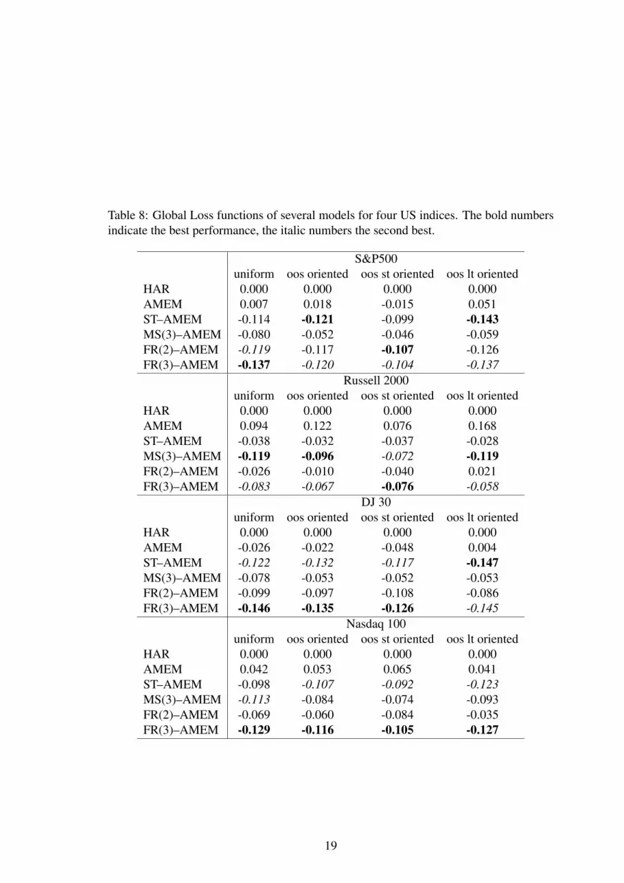
Table 8: Global Loss functions of several models for four US indices. The bold numbersindicate the best performance, the italic numbers the second best.

S&P500uniform oos oriented oos st oriented oos lt oriented

HAR 0.000 0.000 0.000 0.000AMEM 0.007 0.018 -0.015 0.051ST–AMEM -0.114 -0.121 -0.099 -0.143MS(3)–AMEM -0.080 -0.052 -0.046 -0.059FR(2)–AMEM -0.119 -0.117 -0.107 -0.126FR(3)–AMEM -0.137 -0.120 -0.104 -0.137

Russell 2000uniform oos oriented oos st oriented oos lt oriented

HAR 0.000 0.000 0.000 0.000AMEM 0.094 0.122 0.076 0.168ST–AMEM -0.038 -0.032 -0.037 -0.028MS(3)–AMEM -0.119 -0.096 -0.072 -0.119FR(2)–AMEM -0.026 -0.010 -0.040 0.021FR(3)–AMEM -0.083 -0.067 -0.076 -0.058

DJ 30uniform oos oriented oos st oriented oos lt oriented

HAR 0.000 0.000 0.000 0.000AMEM -0.026 -0.022 -0.048 0.004ST–AMEM -0.122 -0.132 -0.117 -0.147MS(3)–AMEM -0.078 -0.053 -0.052 -0.053FR(2)–AMEM -0.099 -0.097 -0.108 -0.086FR(3)–AMEM -0.146 -0.135 -0.126 -0.145

Nasdaq 100uniform oos oriented oos st oriented oos lt oriented

HAR 0.000 0.000 0.000 0.000AMEM 0.042 0.053 0.065 0.041ST–AMEM -0.098 -0.107 -0.092 -0.123MS(3)–AMEM -0.113 -0.084 -0.074 -0.093FR(2)–AMEM -0.069 -0.060 -0.084 -0.035FR(3)–AMEM -0.129 -0.116 -0.105 -0.127

19

Figure 1: Theoretical behavior of the LAV in regime 1 (lower curve) and regime 2 (uppercurve) in correspondence of the smooth transition function gt. The gray area representsthe fuzzy zone. Parameter values: ω = 1, k2 = 3, α0 = 0.5, α1 = 0.4, β0 = 0, β1 = 0,γ0 = 0, γ1 = 0.

20

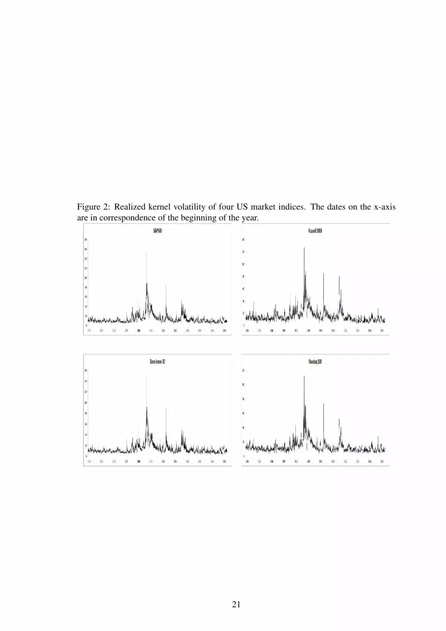
Figure 2: Realized kernel volatility of four US market indices. The dates on the x-axisare in correspondence of the beginning of the year.

21

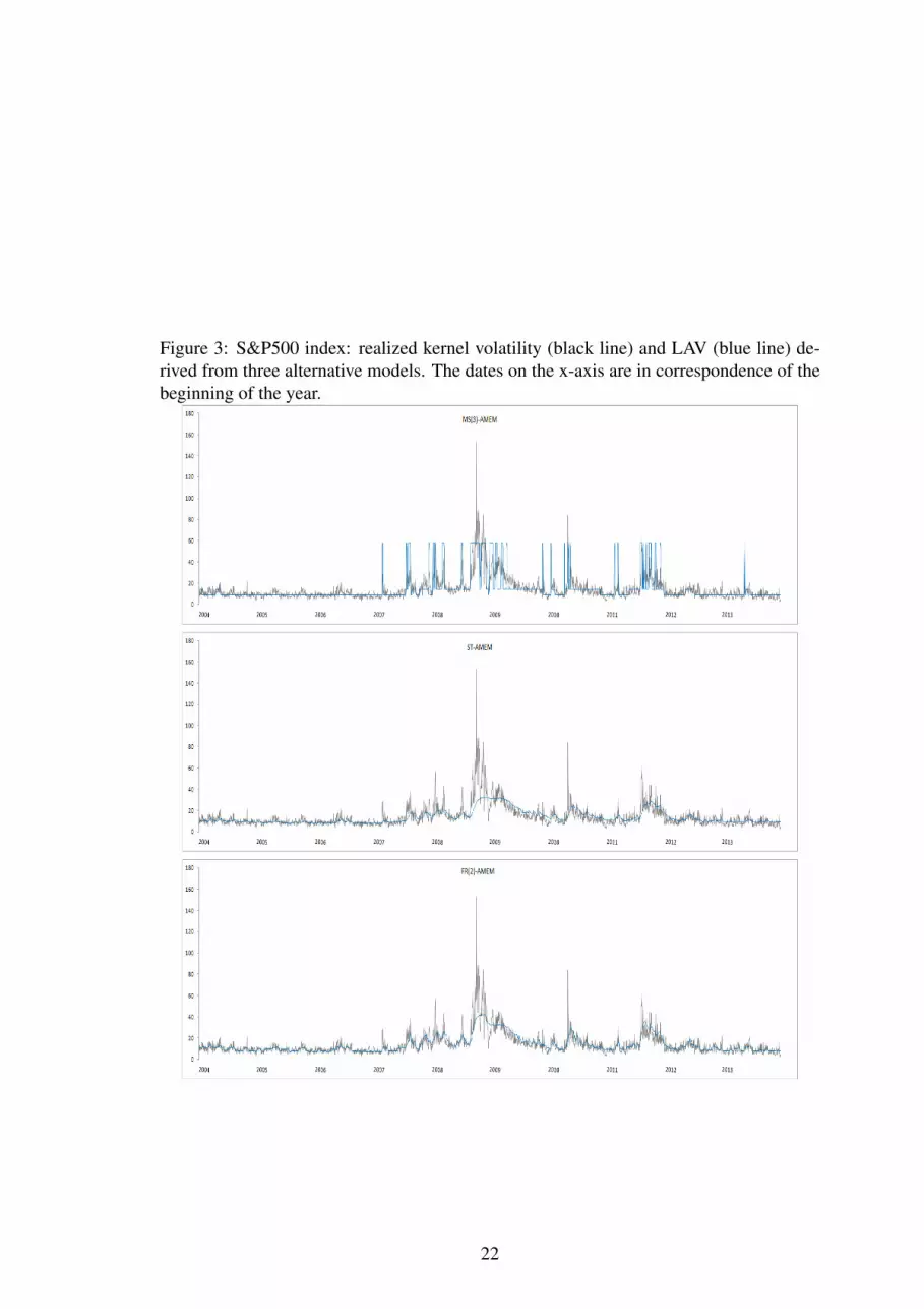
Figure 3: S&P500 index: realized kernel volatility (black line) and LAV (blue line) de-rived from three alternative models. The dates on the x-axis are in correspondence of thebeginning of the year.

22

Figure 4: S&P500 index: Distribution of the realized volatility in terms of regimes derivedfrom the MS(3)–AMEM and the FR(2)–AMEM.

23

Figure 5: S&P500 index: realized kernel volatility and inference on the regime (rightaxis), distinguishing fuzzy regimes (blue dotted line) and crisp regimes (black continu-ous line); the results are derived from a FR(2)–AMEM. The dates on the x-axis are incorrespondence of the beginning of the year.

24

Documents

Combining Markov Switching and Smooth Transition in Modeling Volatility: A Fuzzy Regime MEM