Embed Size (px)
Citation preview
arX
iv:0
911.
2171
v3 [
mat
h.O
C]
3 A
ug 2
010
Combinatorial Characterizations
of K-matricesa
Jan Foniokbc
Komei Fukudabde
Lorenz Klausbf
August 4, 2010
We present a number of combinatorial characterizations of K-matrices.This extends a theorem of Fiedler and Ptak on linear-algebraic character-izations of K-matrices to the setting of oriented matroids. Our proof iselementary and simplifies the original proof substantially by exploiting theduality of oriented matroids. As an application, we show that a simpleprincipal pivot method applied to the linear complementarity problems withK-matrices converges very quickly, by a purely combinatorial argument.
Key words: P-matrix, K-matrix, oriented matroid, linear complementarity2010 MSC: 15B48, 52C40, 90C33
1 Introduction
A matrix M ∈ Rn×n is a P-matrix if all its principal minors (determinants of principalsubmatrices) are positive; it is a Z-matrix if all its off-diagonal elements are non-positive;and it is a K-matrix if it is both a P-matrix and a Z-matrix.
Z- and K-matrices often occur in a wide variety of areas such as input–output produc-tion and growth models in economics, finite difference methods for partial differentialequations, Markov processes in probability and statistics, and linear complementarityproblems in operations research [2].
In 1962, Fiedler and Ptak [9] listed thirteen equivalent conditions for a Z-matrix tobe a K-matrix. Some of them concern the sign structure of vectors:
a
This research was partially supported by the project ‘A Fresh Look at the Complexity of Pivoting inLinear Complementarity’ no. 200021-124752 / 1 of the Swiss National Science Foundation.
b
ETH Zurich, Institute for Operations Research, 8092 Zurich, Switzerlandc
ETH Zurich, Institute of Theoretical Computer Science, 8092 Zurich, Switzerlande
1
Theorem 1.1 (Fiedler–Ptak [9]). Let M be a Z-matrix. Then the following conditionsare equivalent:(a) There exists a vector x ≥ 0 such that Mx > 0;(b) there exists a vector x > 0 such that Mx > 0;(c) the inverse M−1 exists and M−1 ≥ 0;(d) for each vector x 6= 0 there exists an index k such that xkyk > 0 for y = Mx;(e) all principal minors of M are positive (that is, M is a P-matrix, and thus a
K-matrix).
Our interest in K-matrices originates in the linear complementarity problem (LCP),which is for a given matrix M ∈ Rn×n and a given vector q ∈ Rn to find two vectors wand z in Rn so that
w −Mz = q,
w, z ≥ 0,
wTz = 0.
(1)
In general, the problem to decide whether a LCP has a solution is NP-complete [6, 15].If the matrix M is a P-matrix, however, a unique solution to the LCP always exists [24].Nevertheless, no polynomial-time algorithm to find it is known, nor are hardness resultsfor this intriguing class of LCPs. It is unlikely to be NP-hard, because that would implythat NP = co-NP [18]. Recognizing whether a matrix is a P-matrix is co-NP-complete [8].For some recent results, see also [20].
If the matrix M is a Z-matrix, a polynomial-time (pivoting) algorithm exists [5] (seealso [23, sect. 8.1]) that finds the solution or concludes that no solution exists. Interest-ingly, LCPs over this simple class of matrices have many practical applications (pricingof American options, portfolio selection problems, resource allocation problems).
A frequently considered class of algorithms to solve LCPs is the class of simple principalpivoting methods (see Section 6 or [7, Sect. 4.2]). We speak about a class of algorithmsbecause the concrete algorithm depends on a chosen pivot rule. It has recently beenproved in [11] that a simple principal pivoting method with any pivot rule takes at mosta number of pivot steps linear in n to solve a LCP with a K-matrix M .
The study of pivoting methods and pivot rules has led to the devising of combinatorialabstractions of LCPs. One such abstraction is unique-sink orientations of cubes [25]; theone we are concerned with here is one of oriented matroids.
Oriented matroids were pioneered by Bland and Las Vergnas [4] and Folkman andLawrence [10]. Todd [26] and Morris [19] gave a combinatorial generalization of LCPsby formulating the complementarity problem of oriented matroids (OMCP). Morris andTodd [21] studied properties of matroids extending LCPs with symmetric and positivedefinite matrices. Todd [26] proposed a generalization of Lemke’s method [16] to solvethe OMCP. Later Klafszky and Terlaky [14] and Fukuda and Terlaky [12] proposed ageneralized criss-cross method; in [12] it is used for a constructive proof of a dualitytheorem for OMCPs in sufficient matroids (and hence also for LCPs with sufficientmatrices). Hereby we revive their approach.
In this paper, we present a combinatorial generalization (Theorem 5.4) of the Fiedler–Ptak Theorem 1.1. To this end, we devise oriented-matroid counterparts of the con-
2
ditions (a)–(d). If the oriented matroid in question is realizable as the sign pattern ofthe null space of a matrix, then our conditions are equivalent to the conditions on therealizing matrix. In general, however, our theorem is stronger because it applies also tononrealizable oriented matroids.
As a by-product, our proof yields a new, purely combinatorial proof of Theorem 1.1.Rather than on algebraic properties, it relies heavily on oriented matroid duality.
We then use our characterization theorem to show that an OMCP on an n-dimensionalK-matroid (that is, a matroid satisfying the equivalent conditions of Theorem 5.4) issolved by any pivoting method in at most 2n pivot steps. This implies the result of [11]mentioned above that any simple principal pivoting method is fast for K-matrix LCPs.
2 Oriented matroids
The theory of oriented matroids provides a natural concept which not only generalizescombinatorial properties of many geometric configurations but presents itself in manyother areas as well, such as topology and theoretical chemistry.
2.1 Definitions and basic properties
Here we state the definitions and basic properties of oriented matroids that we need inour exposition. For more on oriented matroids consult, for instance, the book [3].
Let E be a finite set of size n. A sign vector on E is a vector X in {+1, 0,−1}E.Instead of +1, we write just +; instead of −1, we write just −. We define X− ={e ∈ E : Xe = −}, X⊖ = {e ∈ E : Xe = − or Xe = 0}, and the sets X0, X⊕ and X+
analogously. For any subset F of E we write XF ≥ 0 if F ⊆ X⊕, and XF ≤ 0 ifF ⊆ X⊖; furthermore X ≥ 0 if XE ≥ 0 and X ≤ 0 if XE ≤ 0. The support of a signvector X is X = X+∪X−. The opposite of X is the sign vector −X with (−X)+ = X−,(−X)− = X+ and (−X)0 = X0. The composition of two sign vectors X and Y is givenby
(X ◦ Y )e =
{
Xe if Xe 6= 0,
Ye otherwise.
The product X · Y of two sign vectors is the sign vector given by
(X · Y )e =
0 if Xe = 0 or Ye = 0,
+ if Xe = Ye and Xe 6= 0,
− otherwise.
Definition 2.1. An oriented matroid on E is a pair M = (E,V), where V is a set ofsign vectors on E satisfying the following axioms:(V1) 0 ∈ V.(V2) If X ∈ V, then −X ∈ V.(V3) If X,Y ∈ V, then X ◦ Y ∈ V.
3
(V4) If X,Y ∈ V and e ∈ X+ ∩ Y −, then there exists Z ∈ V with Z+ ⊆ X+ ∪ Y +,Z− ⊆ X− ∪ Y −, Ze = 0, and (X \ Y ) ∪ (Y \X) ∪ (X+ ∩ Y +) ∪ (X− ∪ Y −) ⊆ Z.
The axioms (V1) up to (V4) are called vector axioms; (V4) is the vector eliminationaxiom. We say that the sign vector Z is the result of a vector elimination of X and Yat element e.
An important example is a matroid whose vectors are the sign vectors of elements ofa vector subspace of Rn. If A is an r × n real matrix, define
V = {sgn x : x ∈ Rn and Ax = 0}, (2)
where sgnx = (sgn x1, . . . , sgnxn). Then V is the vector set of an oriented matroid onthe set E = {1, 2, . . . , n}. In this case we speak of realizable oriented matroids.
A circuit of M is a nonzero vector C ∈ V such that there is no nonzero vector X ∈ Vsatisfying X ⊂ C.
Proposition 2.2. Let M = (E,V) be a matroid and let C be the collection of all itscircuits. Then:(C1) 0 6∈ C.(C2) If C ∈ C, then −C ∈ C.(C3) For all C,D ∈ C, if C ⊆ D, then C = D or C = −D.(C4) If C,D ∈ C, C 6= −D and e ∈ C+ ∩ D−, then there is a Z ∈ C with Z+ ⊆
(C+ ∪D+) \ {e} and Z− ⊆ (C− ∪D−) \ {e}.(C5) If C,D ∈ C, e ∈ C+ ∩D− and f ∈ (C+ \D−) ∪ (C− \D+), then there is a Z ∈ C
with Z+ ⊆ (C+ ∪D+) \ {e}, Z− ⊆ (C− ∪D−) \ {e} and Zf 6= 0.(C6) For every vector X ∈ V there exist circuits C1, C2, . . . , Ck ∈ C such that X =
C1 ◦ C2 ◦ · · · ◦ Ck and Cie · C
je ≥ 0 for all indices i, j and all e ∈ X.
Moreover, if a set C of sign vectors on E satisfies (C1)–(C4), then it is the set of allcircuits of a unique matroid; this matroid’s vectors are then all finite compositions ofcircuits from C.
The property (C4) is called weak circuit elimination; (C5) is called strong circuitelimination. In (C6) we speak about a conformal decomposition of a vector into circuits.
A basis of an oriented matroid M is an inclusion-maximal set B ⊆ E for which thereis no circuit C with C ⊆ B. Every basis B has the same size, called the rank of M.
Proposition 2.3. Let B be a basis of an oriented matroid M. For every e in E \ Bthere is a unique circuit C(B, e) such that C(B, e) ⊆ B ∪ {e} and C(B, e)e = +.
Such a circuit C(B, e) is called the fundamental circuit of e with respect to B.
Two sign vectors X and Y are orthogonal if the set {Xe · Ye : e ∈ E} either equals {0}or contains both + and −. We then write X ⊥ Y .
Proposition 2.4. For every oriented matroid M = (E,V) of rank n there is a uniqueoriented matroid M∗ = (E,V∗) of rank |E| − n given by
V∗ ={
Y ⊆ {−, 0,+}E : X ⊥ Y for every X ∈ V}
.
4
This M∗ is called the dual of M. Note that (M∗)∗ = M. The circuits of M∗ arecalled the cocircuits of M and the vectors of M∗ are called the covectors of M. Thecovectors of a realizable matroid given by (2) are sign vectors of the elements of the rowspace of the matrix A.
We conclude this short overview by introducing the concept of matroid minors andextensions. For any F ⊆ E, the vector X \ F denotes the subvector (Xe : e ∈ E \ F )of X. Then let
V \ F = {X \ F : X ∈ V and Xf = 0 for all f ∈ F}
be the deletion andV/F = {X \ F : X ∈ V}
the contraction of the vectors in V by the elements of F . It is easy to check that thepairs M\ F = (E \ F,V \ F ) and M/F = (E \ F,V/F ) are oriented matroids. For anydisjoint F,G ⊆ E we call the oriented matroid (M\ F )/G a minor of M.
Note that M\{e, e′} = (M\ {e}) \ {e′}, M/{e, e′} = (M/{e})/{e′} and (M\ {e})/{e′} = (M/{e′}) \ {e}, and so deletions and contractions can be performed element byelement in any order, with the same result.
Definition 2.5. A matroid M = (E∪{q} , V) with q 6∈ E is a one-point extension of Mif M \ {q} = M and there is a vector X of M with Xq 6= 0.
2.2 Complementarity in oriented matroids
In the rest of the paper, we are considering oriented matroids endowed with a specialstructure. The set of elements E2n is a 2n-element set with a fixed partition E2n = S∪Tinto two n-element sets and a mapping e 7→ e from E2n to E2n which is an involution(that is, e = e for every e ∈ E2n) and for every e ∈ S we have e ∈ T . Note that thismapping constitutes a bijection between S and T .
The element e is called the complement of e. For a subset F of E2n let F = {e : e ∈ F}.A subset F of E2n is called complementary if F ∩ F = ∅.
The matroids we are working with are of the kind M = (E2n,V), where the setS ⊆ E2n is a basis of M. In addition, we study their one-point extensions M = (E2n, V),where E2n = E2n ∪ {q} for some element q /∈ E2n. Sometimes we make the canonicalchoice E2n = {1, . . . , 2n} with S = {1, . . . , n} where the complement of an i ∈ S is theelement i+ n.
Definition 2.6. The oriented matroid complementarity problem (OMCP) is to find avector X of an oriented matroid M so that
X ∈ V, (3a)
X ≥ 0, Xq = +, (3b)
Xe ·Xe = 0 for every e ∈ E2n, (3c)
or to report that no such vector exists.
5
A vector X which satisfies (3b) is called feasible, one which satisfies (3c) is calledcomplementary. Note that a vector is complementary if and only if its support is acomplementary set. If an X ∈ V satisfies (3b) and (3c), then X is a solution to theOMCP(M).
Now we show how LCPs are special cases of OMCPs. Finding a solution to theLCP (1) is equivalent to finding an element x of
V ={
x ∈ R2n+1 :[
In −M −q]
x = 0}
such thatx ≥ 0, x2n+1 = 1,
xi · xi+n = 0 for every i ∈ [n] .(4)
We set V = {sgnx : x ∈ V } and consider the OMCP for the matroid M = (E2n, V).Clearly, if the OMCP has no solution, then V contains no vector x satisfying (4). If onthe other hand there is a solution X satisfying (3a)–(3c), then the solution to the LCPcan be obtained by solving the system of linear equations
[
In −M −q]
x = 0,
xi = 0 whenever Xi = 0,
x2n+1 = 1.
This correspondence motivates the following definition.
Definition 2.7. An oriented matroid M = (E2n,V) is LCP-realizable if there is a matrixM ∈ Rn×n such that
V ={
sgnx : x ∈ R2n and[
In −M]
x = 0}
.
The matrix M is then a realization matrix of M. This is a little nonstandard, becauseusually the matrix A from (2) is called a realization matrix. The columns of In areindexed by the elements of S ⊂ E2n, and the columns of −M are indexed by the elementsof T ⊂ E2n so that if the kth column of In is indexed by e, then the kth column of −Mis indexed by e.
The extension M = (E2n, V) is LCP-realizable if there is a matrix M ∈ Rn×n and avector q ∈ Rn such that
V ={
sgnx : x ∈ R2n+1 and[
In −M −q]
x = 0}
.
To study the algorithmic complexity of OMCPs, we must specify how the matroid Mis made available to the algorithm. We will assume that it is given by an oracle which, fora basis B of M and a nonbasic element e ∈ E2n \B, outputs the unique (fundamental)circuit C of M with support C ⊆ B ∪ {e} such that Xe = +.
In the LCP-realizable case such an oracle can be implemented in polynomial time;in fact, it consists in solving a system of O(n) linear equations in 2n + 1 variables.
6
Thus, in the RAM model, the oracle can be implemented so that it performs arithmeticoperations whose number is bounded by a polynomial in n. Hence our goal is to developan algorithm that solves an OMCP using a number of queries to the oracle that ispolynomial in n.
Such an algorithm for the OMCP would obviously provide a strongly polynomialalgorithm for the LCP. Since the LCP is NP-hard in general, the existence of such analgorithm is unlikely. In Section 6 we do, nevertheless, prove the existence of such analgorithm for a special class of oriented matroids: K-matroids.
3 P-matroids
In this and the following sections, we investigate what properties of oriented matroidscharacterize oriented matroids realizable by special classes of matrices. We start withP-matrices; recall that a P-matrix is a matrix whose principal minors are all positive.
Several conditions are equivalent to the positivity of principal minors:
Theorem 3.1. For a matrix M ∈ Rn×n, the following are equivalent:(a) All principal minors of M are positive (i.e., M is a P-matrix);(b) there is no nonzero vector x such that xkyk ≤ 0 for all i = 1, 2, . . . , n, where
y = Mx;(c) the LCP (1) with the matrix M and any right-hand side q has exactly one solution.
The equivalence of (a) and (b) is due to Fiedler and Ptak [9]. The equivalence of (a)and (c) was proved independently by Samelson, Thrall and Wesler [24], Ingleton [13],and Murty [22].
The following notions and our definition of a P-matroid are motivated by the condi-tion (b) in Theorem 3.1. It is much easier to express in the oriented-matroid languagethan (a).
A sign vector X ∈ {−, 0,+}E2n is sign-reversing (s.r.) if Xe ·Xe ≤ 0 for every e ∈ S.If in addition X = E2n, the vector is totally sign-reversing (t.s.r.). Analogously, an Xis sign-preserving (s.p.) if Xe ·Xe ≥ 0 for every e, and totally sign-preserving (t.s.p.) ifX = E2n as well.
Definition 3.2 (Todd [26]). An oriented matroid M on E2n is a P-matroid if it has nosign-reversing circuit.
Note that a P-matroid contains no nonzero sign-reversing vectors, because every vectoris the composition of some circuits and composing non-s.r. circuits yields non-s.r. vectors.Hence, using Theorem 3.1, we immediately get:
Proposition 3.3.
(i) If M is LCP-realizable and there exists a realization matrix M that is a P-matrix,then M is a P-matroid.
(ii) If M is an LCP-realizable P-matroid, then every realization matrix M is a P-matrix.
7
P-matroids were extensively studied by Todd [26]. He lists eight equivalent conditionsfor a matroid to be a P-matroid. We recall three of them (conditions (a), (a*) and (c)below) and add two new ones.
Theorem 3.4. For an oriented matroid M on E2n, the following conditions are equiv-alent:(a) M has no s.r. circuit;
(a*) M has no s.p. cocircuit;(b) every t.s.p. X is a vector of M;
(b*) every t.s.r. Y is a covector of M;(c) every one-point extension M of M to E2n contains exactly one complementary
circuit C such that C ≥ 0 and Cq = +.
Proof. The equivalence of the conditions (a), (a*) and (c) was shown by Todd [26].Morris [19] proved that (a) implies (b). We show the equivalence of (a) with (b*). Theequivalence of (a*) with (b) is proved analogously.
First we prove that (a) implies (b*). Since no circuit of M is s.r., there is for everycircuit C an element e such that Ce · Ce = +. It follows that every t.s.r. sign vector Yis orthogonal to every circuit, hence Y is a covector.
For the opposite direction, suppose that there is a s.r. circuit C. If so, then anyt.s.r. vector Y for which Y + ⊆ C+ and Y − ⊆ C− is not orthogonal to C, which is acontradiction with (b*).
The condition (b) of this theorem has a translation for realization matrices of P-ma-troids, that is, for P-matrices:
Corollary 3.5. A matrix M ∈ Rn×n is a P-matrix if and only if for every σ ∈ {−1,+1}n
there exists a vector x ∈ Rn such that for y = Mx and for each i ∈ {1, 2, . . . , n} we have
σixi > 0,
σiyi > 0.
Todd [26] also gives an oriented-matroid analogue of the “positive principal minors”condition. Stating it would require some more explanations; later in this article we needa weaker property of P-matroids, though, which corresponds to the fact that all principalminors of a P-matrix are nonzero.
Lemma 3.6 (Todd [26]). For a P-matroid M every complementary subset B ⊆ E2n ofcardinality n is a basis.
Remark. In addition, every such complementary B is also a cobasis, i.e., it is a basisof the dual matroid M∗.
Next we consider principal pivot transforms (see [27, 28]) of P-matrices. The fact thatevery principal pivot transform of a P-matrix is again a P-matrix [29] is well-known.The proof is not very difficult but it uses involved properties of the Schur complement.In the setting of oriented matroids the equivalent is much simpler. First let us defineprincipal pivot transforms of oriented matroids.
8
Definition 3.7. Let F ⊆ E2n be a complementary set. The principal pivot transformof a sign vector X with respect to F is the sign vector C given by
Ce =
{
Ce if e /∈ F,
Ce if e ∈ F.
The principal pivot transform of a matroid M with respect to F is the matroid whosecircuits (vectors) are the principal pivot transforms of the circuits (vectors) of M.
It is easy to see that, in the LCP-realizable case, principal pivot transforms of amatroid correspond to matroids realized by corresponding principal pivot transforms ofthe realization matrix. Thus the following proposition implies the analogous theoremfor P-matrices.
Proposition 3.8. Every principal pivot transform of a P-matroid is a P-matroid.
Proof. The principal pivot transform of a circuit C is sign-reversing if and only if C issign-reversing.
4 Z-matroids
The second class of matrices we examine are Z-matrices; the corresponding matroidgeneralizations are Z-matroids. Recall that a Z-matrix is a matrix whose every off-diagonal element is non-positive. The definition of Z-matroids was first proposed in [17].
Definition 4.1. A matroid M on E2n is a Z-matroid if for every circuit C of M wehave:
If CT ≥ 0, then
Ce = + for all e ∈ S with Ce = +.(5)
Remark. In the definition of Z-matroid we could replace all occurrences of the word“circuit” with the word “vector”. Indeed, in a conformal decomposition of a vectorviolating (5), there would always be a circuit violating (5) as well.
It makes perfect sense to define Z-matroids in this way. We show that in LCP-realizable cases, any realization matrix M is a Z-matrix.
Proposition 4.2.
(i) If M is LCP-realizable and there exists a realization matrix M that is a Z-matrix,then M is a Z-matroid.
(ii) If M is an LCP-realizable Z-matroid, then every realization matrix M is a Z-matrix.
Proof. We fix E2n = {1, . . . , 2n} with S = {1, . . . , n} where the complement of an i ∈ Sis the element i+ n.
9
(i) Let ei denote the ith unit vector and mj the jth column of the matrix M . Thesign pattern of the Z-matrix M implies that there is no linear combination of the form
ei +
n∑
j=1
j 6=i
xjej −2n∑
j=n+1
xjmj = 0,
where xj ≥ 0 for every j > n and xi+n = 0, because the ith row of the left-hand sideis strictly positive. Hence there is no vector X ∈ V for which XT ≥ 0, Xi = + butXi+n = 0 for some i ∈ S.
(ii) Proof by contradiction. Assume that for an LCP-realizable Z-matroid M (whereS is a basis), there is a realization matrix M that is not a Z-matrix, that is, there is anoff-diagonal mij > 0. If so, there is a vector X with Xj+n = + and XT\{j+n} = 0, butXi = +. ThisX violates the Z-matroid property (5) since alsoXi+n = 0, a contradiction.Thus no positive mij can exist and M has to be a Z-matrix.
Another option is to characterize a Z-matroid with respect to the dual matroid M∗.
Proposition 4.3. An oriented matroid M on E2n is a Z-matroid if and only if for everycocircuit D of M we have:
If DS ≤ 0, then
De = − for all e ∈ T with De = +.(6)
Proof. First we prove the “only if” direction. Suppose that there is a cocircuit D whichdoes not satisfy (6). Accordingly DS ≤ 0 and there is e ∈ T such that De = +, butDe = 0. But note that the fundamental circuit C := C(S, e) and D are not orthogonalbecause the Z-matroid property (5) implies that CS\{e} ≤ 0. Hence no such D can exist.
For the “if” direction suppose that there is a circuit C for which CT ≥ 0 and Ce = +,but Ce = 0 for some e ∈ S. This circuit C and the fundamental cocircuit D := D(T, e)are not orthogonal since by assumption (6) holds forD and of course−D, henceDT\{e} ≥0.
In the proofs in the following section we often make use of fundamental circuits. Herewe observe that all fundamental circuits with respect to the basis S follow the same signpattern.
Lemma 4.4. Let M be a Z-matroid. Let e ∈ T and let C = C(S, e) be the fundamentalcircuit of e with respect to the basis S. Then
Ce = +,
CT\{e} = 0,
CS\{e} ≤ 0.
Proof. The first and the second equality follow directly from the definition of a funda-mental circuit. Thus CT ≥ 0. Hence the third property follows from the Z-matroidproperty (5).
10
5 K-matroids
Definition 5.1. A matroid M on E2n is a K-matroid if it is a P-matroid and a Z-matroid.
Combining Proposition 3.3 and Proposition 4.2 we immediately get:
Proposition 5.2.
(i) If M is LCP-realizable and there exists a realization matrix M that is a K-matrix,then M is a K-matroid.
(ii) If M is an LCP-realizable K-matroid, then every realization matrix M is a K-matrix.
An oriented matroid minor M \ F/F where F is a complementary subset of E2n iscalled a principal minor of M.
Lemma 5.3. Let M be a K-matroid. Then every principal minor M \ F/F is a K-matroid.
Proof. It was shown by Todd [26] that every principal minor of a P-matroid is a P-matroid. Thus, it is enough to show that such a minor is a Z-matroid, and for this, sincedeletions and contractions can be carried out element by element in any order, it sufficesto consider the case that F is a singleton.
First, we prove that if e ∈ T , then M \ {e} / {e} is a Z-matroid. Such a principalminor consists of all circuits C \ {e, e}, where C is a circuit of M and Ce = 0. Sinceevery circuit of M satisfies the Z-matroid characterization (5), such a circuit C \ {e, e}trivially satisfies it too.
Secondly, let e ∈ S. Here we apply a case distinction. If Ce = +, then (C \{e, e})T ≥ 0if and only if CT ≥ 0. As a direct consequence, C \ {e, e} satisfies (5) because C does.If Ce = −, we can show that there is another element f ∈ T such that Cf = − too,that is, (C \ {e, e})T 6≥ 0 and thus the Z-matroid property (5) is obviously satisfied.Assume for the sake of contradiction that there is no such f ∈ T . The strong circuitelimination (C5) of C and the fundamental circuit C(S, e) at e then yields a circuit C ′
with C ′T ≥ 0, C ′
e = 0 and C ′e = +. Since e ∈ S, such a C ′ would violate the Z-matroid
definition, a contradiction.
Our main result, the combinatorial generalization of the Fiedler–Ptak Theorem 1.1 isthe following.
Theorem 5.4. For a Z-matroid M (with vectors V, covectors V∗, circuits C and cocir-cuits D), the following statements are equivalent:
(a) ∃X ∈ V : XT ≥ 0 and XS > 0; (a*) ∃Y ∈ V∗ : YS ≤ 0 and YT > 0;(b) ∃X ∈ V : X > 0; (b*) ∃Y ∈ V∗ : YS < 0 and YT > 0;(c) ∀C ∈ C: CS ≥ 0 =⇒ CT ≥ 0; (c*) ∀D ∈ D: DT ≥ 0 =⇒ DS ≤ 0;(d) there is no s.r. circuit C ∈ C (d*) there is no s.p. cocircuit D ∈ D.
(that is, M is a P-matroid);
11
In order to use duality in the proof of this theorem, let us first define the reflection ofa matroid M = (E2n,V) to be the matroid ℜ(M) = (E2n,ℜ(V)), where ℜ(V) = {ℜ(X) :X ∈ V} with
(
ℜ(X))
e=
{
Xe if e ∈ S,
−Xe if e ∈ T .
Observe that ℜ(
ℜ(M))
= M because of (V2), and that ℜ(M∗) = ℜ(M)∗; thus
ℜ(
ℜ(M∗)∗)
= M. (7)
Proof of Theorem 5.4.
(a) =⇒ (b): Let X be as in (a). Since XT ≥ 0, the Z-matroid property (5) impliesthat if Xe = + for an e ∈ S, then Xe = +. Thus XT > 0.
(b) =⇒ (c): Let X be the all-plus vector as in (b). Suppose that there is a circuitC ∈ C not satisfying (c), that is, CS ≥ 0 but Ce = − for some element e in T .Starting with Y 0 = C, we apply a sequence of vector eliminations (V4) to getvectors Y i. We eliminate Y i−1 and X at any element e where Y i−1
e = −. For aresulting vector Y i it holds that (Y i)− ⊂ (Y i−1)−. Thus, at some point (Y k)− = ∅while Y k
e = 0 and Y ke = + where e ∈ T is the element eliminated in step k−1. This
vector Y k does not satisfy the Z-matroid property (5), which is a contradiction.
(c) =⇒ (d): Suppose that there is a s.r. circuit C ∈ C, that is, Ce · Ce ≤ 0 for everye ∈ S. Let C0 = C. We apply consecutive circuit eliminations (C4). To get Ci, weeliminate Ci−1 with any fundamental circuit C := C(S, e) at position e ∈ T whereCi−1e = −. By Lemma 4.4 we have CS\{e} ≤ 0.
After finitely many eliminations we end up with a circuit Ck for which CkT ≥ 0.
Now we claim that CkS ≤ 0: Indeed, if e ∈ S such that Ck
e = +, then Ce = +,and thus Ce ≤ 0 because C is sign-reversing. Since we never eliminate at e, allfundamental circuits C used in the eliminations satisfy Ce ≤ 0 as noted above.Hence Ck
e ≤ 0. If on the other hand Cke = 0, then Ck
e ≤ 0 by (5).
Moreover, since S is a basis, Ck * S, and so there exists e ∈ T with Cke = +.
Therefore −Ck violates property (c), a contradiction.
(d) =⇒ (a*): Because of (d), for every circuit C there is an e ∈ S such that Ce ·Ce = +.The sign vector Y where YS < 0 and YT > 0 is orthogonal to every circuit C,because the sign of Ye · Ce is opposite to the sign of Ye · Ce. Hence such a Y is acovector.
To finish the proof, notice that a matroid M satisfies (a*) if and only if the reflectionof its dual ℜ(M∗) satisfies (a); analogously for (b*) and (b), (c*) and (c), and (d*)and (d). Thus if M satisfies (a*), then ℜ(M∗) satisfies (a), hence also (b), and so(using (7)) M satisfies (b*). The missing implications (b*) =⇒ (c*), (c*) =⇒ (d*),and (d*) =⇒ (a) are proved analogously.
12
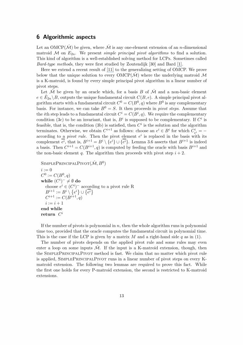
6 Algorithmic aspects
Let an OMCP(M) be given, where M is any one-element extension of an n-dimensionalmatroid M on E2n. We present simple principal pivot algorithms to find a solution.This kind of algorithm is a well-established solving method for LCPs. Sometimes calledBard-type methods, they were first studied by Zoutendijk [30] and Bard [1].
Here we extend a recent result of [11] to the generalizing setting of OMCP. We provebelow that the unique solution to every OMCP(M) where the underlying matroid Mis a K-matroid, is found by every simple principal pivot algorithm in a linear number ofpivot steps.
Let M be given by an oracle which, for a basis B of M and a non-basic elemente ∈ E2n\B, outputs the unique fundamental circuit C(B, e). A simple principal pivot al-gorithm starts with a fundamental circuit C0 = C(B0, q) whereB0 is any complementarybasis. For instance, we can take B0 = S. It then proceeds in pivot steps. Assume thatthe ith step leads to a fundamental circuit Ci = C(Bi, q). We require the complementarycondition (3c) to be an invariant, that is, Bi is supposed to be complementary. If Ci isfeasible, that is, the condition (3b) is satisfied, then Ci is the solution and the algorithmterminates. Otherwise, we obtain Ci+1 as follows: choose an ei ∈ Bi for which Ci
ei= −
according to a pivot rule. Then the pivot element ei is replaced in the basis with itscomplement ei, that is, Bi+1 = Bi \ {ei} ∪ {ei}. Lemma 3.6 asserts that Bi+1 is indeeda basis. Then Ci+1 = C(Bi+1, q) is computed by feeding the oracle with basis Bi+1 andthe non-basic element q. The algorithm then proceeds with pivot step i+ 2.
SimplePrincipalPivot(M, B0)
i := 0C0 := C(B0, q)while (Ci)− 6= ∅ do
choose ei ∈ (Ci)− according to a pivot rule RBi+1 := Bi \
{
ei}
∪{
ei}
Ci+1 := C(Bi+1, q)i := i+ 1
end while
return Ci
If the number of pivots is polynomial in n, then the whole algorithm runs in polynomialtime too, provided that the oracle computes the fundamental circuit in polynomial time.This is the case if the LCP is given by a matrix M and a right-hand side q as in (1).
The number of pivots depends on the applied pivot rule and some rules may evenenter a loop on some inputs M. If the input is a K-matroid extension, though, thenthe SimplePrincipalPivot method is fast. We claim that no matter which pivot ruleis applied, SimplePrincipalPivot runs in a linear number of pivot steps on every K-matroid extension. The following two lemmas are required to prove this fact. Whilethe first one holds for every P-matroid extension, the second is restricted to K-matroidextensions.
13
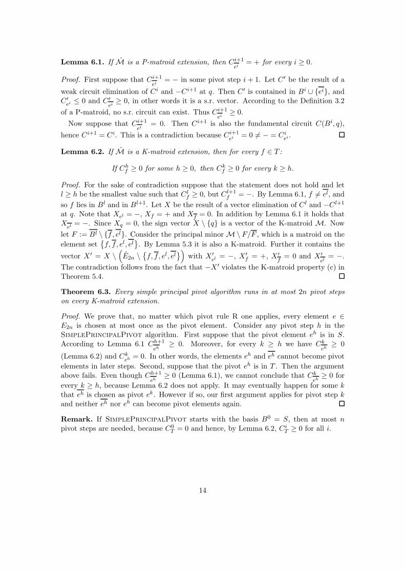
Lemma 6.1. If M is a P-matroid extension, then Ci+1
ei= + for every i ≥ 0.
Proof. First suppose that Ci+1
ei= − in some pivot step i + 1. Let C ′ be the result of a
weak circuit elimination of Ci and −Ci+1 at q. Then C ′ is contained in Bi ∪ {ei}, andC ′ei
≤ 0 and C ′ei
≥ 0, in other words it is a s.r. vector. According to the Definition 3.2
of a P-matroid, no s.r. circuit can exist. Thus Ci+1
ei≥ 0.
Now suppose that Ci+1
ei= 0. Then Ci+1 is also the fundamental circuit C(Bi, q),
hence Ci+1 = Ci. This is a contradiction because Ci+1
ei= 0 6= − = Ci
ei.
Lemma 6.2. If M is a K-matroid extension, then for every f ∈ T :
If Chf ≥ 0 for some h ≥ 0, then Ck
f ≥ 0 for every k ≥ h.
Proof. For the sake of contradiction suppose that the statement does not hold and letl ≥ h be the smallest value such that C l
f ≥ 0, but C l+1
f = −. By Lemma 6.1, f 6= el, and
so f lies in Bl and in Bl+1. Let X be the result of a vector elimination of C l and −C l+1
at q. Note that Xel = −, Xf = + and Xf = 0. In addition by Lemma 6.1 it holds thatX
el= −. Since Xq = 0, the sign vector X \ {q} is a vector of the K-matroid M. Now
let F := Bl \ {f , el}. Consider the principal minor M\ F/F , which is a matroid on the
element set{
f, f, el, el}
. By Lemma 5.3 it is also a K-matroid. Further it contains the
vector X ′ = X \(
E2n \{
f, f, el, el}
)
with X ′el
= −, X ′f = +, X ′
f= 0 and X ′
el= −.
The contradiction follows from the fact that −X ′ violates the K-matroid property (c) inTheorem 5.4.
Theorem 6.3. Every simple principal pivot algorithm runs in at most 2n pivot stepson every K-matroid extension.
Proof. We prove that, no matter which pivot rule R one applies, every element e ∈E2n is chosen at most once as the pivot element. Consider any pivot step h in theSimplePrincipalPivot algorithm. First suppose that the pivot element eh is in S.According to Lemma 6.1 Ch+1
eh≥ 0. Moreover, for every k ≥ h we have Ck
eh≥ 0
(Lemma 6.2) and Ckeh
= 0. In other words, the elements eh and eh cannot become pivot
elements in later steps. Second, suppose that the pivot eh is in T . Then the argumentabove fails. Even though Ch+1
eh≥ 0 (Lemma 6.1), we cannot conclude that Ck
eh≥ 0 for
every k ≥ h, because Lemma 6.2 does not apply. It may eventually happen for some kthat eh is chosen as pivot ek. However if so, our first argument applies for pivot step kand neither eh nor eh can become pivot elements again.
Remark. If SimplePrincipalPivot starts with the basis B0 = S, then at most npivot steps are needed, because C0
T = 0 and hence, by Lemma 6.2, CiT ≥ 0 for all i.
14
7 Extension to principal pivot closures
So far, we have considered a matroid M on a complementary set E2n where the maximalcomplementary set S is fixed from the beginning. In the following, S′ is an arbitrarycomplementary subset of size n and T ′ = {e : e ∈ S′}.
Definition 7.1. A matroid M on E2n is a Z*-matroid if there is a complementary setS′ ⊆ E2n of cardinality n such that for T ′ = {e : e ∈ S′} and every circuit C of M wehave:
If CT ′ ≥ 0, then
Ce = + for all e ∈ S′ with Ce = +.
Analogously M is a K*-matroid if it is a P-matroid and a Z*-matroid. Note that theclass of Z*- and K*-matroids are the closures, under all principal pivot transforms, of Z-and K-matroids, respectively. Moreover, Proposition 4.3, Lemma 5.3 up to Theorem 6.3have equivalent counterparts for these closure classes, obtained by substituting S by S′
and accordingly T by T ′ in the original statements. Hence we get the following.
Corollary 7.2. Every simple principal pivot algorithm finds the solution to OMCP(M),where M is a K*-matroid extension, in at most 2n pivot steps.
The reader might wonder why we introduced Z-matroids and K-matroids at all anddid not start off with their principal pivot closures. One good reason for our approachis to point out the correspondence of LCP-realizable Z-matroids and their matrix coun-terparts, see Proposition 4.2. With respect to this, the main problem is that a principalpivot transform of a Z-matroid or a K-matroid is in general not a Z-matroid, a K-matroidrespectively. However every principal pivot algorithm is still able to solve an LCP(M, q)where M is a principal pivot transform of a K-matrix in a linear number of pivot steps.
References
[1] Yonathan Bard. An eclectic approach to nonlinear programming. In Optimization(Proc. Sem., Austral. Nat. Univ., Canberra, 1971), pages 116–128, St. Lucia, 1972.Univ. Queensland Press.
[2] Abraham Berman and Robert J. Plemmons. Nonnegative matrices in the mathe-matical sciences. Academic Press, 1979.
[3] Anders Bjorner, Michel Las Vergnas, Bernd Sturmfels, Neil White, and Gunter M.Ziegler. Oriented Matroids, volume 46 of Encyclopedia of mathematics and its ap-plications. Cambridge University Press, second edition, 1999.
[4] Robert G. Bland and Michel Las Vergnas. Orientability of matroids. J. Combin.Theory, Ser. B, 24:94–123, 1978.
15
[5] Ramaswamy Chandrasekaran. A special case of the complementary pivot problem.Opsearch, 7:263–268, 1970.
[6] Sung-Jin Chung. NP-completeness of the linear complementarity problem. J. Op-tim. Theory Appl., 60(3):393–399, 1989.
[7] Richard W. Cottle, Jong-Shi Pang, and Richard E. Stone. The Linear Comple-mentarity Problem. Computer science and scientific computing. Academic Press,1992.
[8] Gregory E. Coxson. The P-matrix problem is co-NP-complete. Math. Programming,Ser. A, 64(2):173–178, 1994.
[9] Miroslav Fiedler and Vlastimil Ptak. On matrices with non-positive off-diagonalelements and positive principal minors. Czechoslovak Math. J., 12 (87):382–400,1962.
[10] Jon Folkman and Jim Lawrence. Oriented matroids. J. Combin. Theory, Ser. B,25:199–236, 1978.
[11] Jan Foniok, Komei Fukuda, Bernd Gartner, and Hans-Jakob Luthi. Pivoting inlinear complementarity: Two polynomial-time cases. Discrete Comput. Geom.,42(2):187–205, 2009.
[12] Komei Fukuda and Tamas Terlaky. Linear complementarity and oriented matroids.J. Oper. Res. Soc. Japan, 35(1):45–61, 1992.
[13] Aubrey William Ingleton. A problem in linear inequalities. Proc. London Math.Soc. (3), 16:519–536, 1966.
[14] Emil Klafszky and Tamas Terlaky. Some generalizations of the criss-cross method forthe linear complementarity problem of oriented matroids. Combinatorica, 9(2):189–198, 1989.
[15] Masakazu Kojima, Nimrod Megiddo, Toshihito Noma, and Akiko Yoshise. A unifiedapproach to interior point algorithms for linear complementarity problems, volume538 of Lecture Notes in Computer Science. Springer-Verlag, Berlin, 1991.
[16] Carlton E. Lemke. Bimatrix equilibrium points and mathematical programming.Management Sci., 11:681–689, 1964/1965.
[17] Carlton E. Lemke and Hans-Jakob Luthi. Classes of matroids and complementarity.30 pages manuscript, February 1986.
[18] Nimrod Megiddo. A note on the complexity of P-matrix LCP and computing anequilibrium. RJ 6439, IBM Research, Almaden Research Center, 650 Harry Road,San Jose, California, 1988.
16
[19] Walter D. Morris, Jr. Oriented Matroids and the Linear Complementarity Problem.PhD thesis, Cornell University, Ithaca, 1986.
[20] Walter D. Morris, Jr. and Makoto Namiki. Good hidden P-matrix sandwiches.Linear Algebra Appl., 426(2–3):325–341, 2007.
[21] Walter D. Morris, Jr. and Michael J. Todd. Symmetry and positive definiteness inoriented matroids. European J. Combin., 9(2):121–129, 1988.
[22] Katta G. Murty. On the number of solutions to the complementarity problem andspanning properties of complementary cones. Linear Algebra and Appl., 5:65–108,1972.
[23] Katta G. Murty. Linear Complementarity, Linear and Nonlinear Programming,volume 3 of Sigma Series in Applied Mathematics. Heldermann, Berlin, 1988.
[24] Hans Samelson, Robert M. Thrall, and Oscar Wesler. A partition theorem forEuclidean n-space. Proc. Amer. Math. Soc., 9:805–807, 1958.
[25] Alan Stickney and Layne Watson. Digraph models of Bard-type algorithms for thelinear complementarity problem. Math. Oper. Res., 3(4):322–333, 1978.
[26] Michael J. Todd. Complementarity in oriented matroids. SIAM J. Alg. Disc. Meth.,5:467–485, 1984.
[27] Michael J. Tsatsomeros. Principal pivot transforms: Properties and applications.Linear Algebra Appl., 307(1–3):151–165, 2000.
[28] Albert W. Tucker. A combinatorial equivalence of matrices. In Richard Bellman andMarshall Hall, Jr., editors, Proc. Sympos. Appl. Math., volume 10, pages 129–140.American Mathematical Society, 1960.
[29] Albert W. Tucker. Principal pivotal transforms of square matrices. 1963 SpringMeeting of SIAM, Menlo Park, California, 1963. Abstract in SIAM Review, vol. 5,p. 305.
[30] Guus Zoutendijk. Methods of feasible directions: A study in linear and non-linearprogramming. Elsevier Publishing Co., Amsterdam, 1960.
17


