Embed Size (px)
Citation preview
arX
iv:1
201.
1010
v2 [
astr
o-ph
.CO
] 1
4 M
ar 2
012
CMB lensing and primordial squeezed non-Gaussianity
Ruth Pearson,1 Antony Lewis,1, ∗ and Donough Regan1
1Department of Physics & Astronomy, University of Sussex, Brighton BN1 9QH, UK
(Dated: March 15, 2012)
Squeezed primordial non-Gaussianity can strongly constrain early-universe physics, but it canonly be observed on the CMB after it has been gravitationally lensed. We give a new simple non-perturbative prescription for accurately calculating the effect of lensing on any squeezed primordialbispectrum shape, and test it with simulations. We give the generalization to polarization bispectra,and discuss the effect of lensing on the trispectrum. We explain why neglecting the lensing smooth-ing effect does not significantly bias estimators of local primordial non-Gaussianity, even thoughthe change in shape can be & 10%. We also show how τNL trispectrum estimators can be wellapproximated by much simpler CMB temperature modulation estimators, and hence that there ispotentially a ∼ 10–30% bias due to very large-scale lensing modes, depending on the range of mod-ulation scales included. Including dipole sky modulations can halve the τNL error bar if kinematiceffects can be subtracted using known properties of the CMB temperature dipole. Lensing effects onthe gNL trispectrum are small compared to the error bar. In appendices we give the general resultfor lensing of any primordial bispectrum, and show how any full-sky squeezed bispectrum can bedecomposed into orthogonal modes of distinct angular dependence.
I. INTRODUCTION
A squeezed bispectrum or trispectrum produced by local primordial non-Gaussianity is observable in the CMB,and if observed would give a powerful way to rule out simple single-field inflation models and strongly constraingeneral properties of inflation. The local non-Gaussianity produced in the CMB can be thought of as a modulationof small-scale perturbations by large-scale modes, so over a large overdensity there will be more (or less) small-scalepower than over an underdensity, depending on the sign of the non-Gaussianity. However if we observe the small-scale modes they will be gravitationally lensed, so in the squeezed limit we expect to see a modulation of the lensed
small-scale power spectrum due to large-scale modes. This may be important because lensing smooths out acousticstructures, changing the detailed shape of the bispectrum and trispectrum. Previous work Ref. [1] has shown thatfor the temperature bispectrum due only to local primordial non-Gaussianity, the bias due to this change in shape isvery small. However since the shape is changed, accounting for lensing might be important to correctly identify theform of the non-Gaussianity; for example a different shape which is orthogonal to the unlensed bispectrum will notgenerally be orthogonal to the lensed bispectrum. In this paper we give new simple approximations for the effect oflensing on the squeezed CMB temperature and polarization bispectra which allow the effects to be calculated easily.We test these approximations against simulations, and quantify the importance of the lensing at different levels ofprimordial non-Gaussianity.
Previous work has investigated the lensing bispectrum in detail, its potential bias on local non-Gaussianity estima-tors, and its impact on the variance of the primordial non-Gaussianity estimators [1–4]. The bispectrum producedby lensing turns out to be significant, corresponding to a projection of fNL ∼ 9 onto the local shape, and should bedetectable by Planck. However the effect is easily modelled and subtracted since the detailed shape of the lensingbispectrum is actually very different from the local shape [4]. Here we address the different issue of how lensing affectsany other primordial bispectrum that we might want to observe, and assess whether the change due to lensing isimportant.
We then extend to trispectrum estimators, and estimate the bias on local τNL and gNL trispectrum shape due tolensing. We show how this can be calculated easily using simple approximations for the CMB trispectra, and thenalso discuss the effect of lensing on any primordial local trispectrum. The lensing trispectrum is large, and can bedetected at high significance with Planck, but we shall see that its distinctive shape and scale dependence is verydifferent from local primordial non-Gaussianity. We show that although the projection of the lensing shape onto thelocal primordial shapes gives a signal that is much larger than would be expected in most inflationary models, it isstill only a small-fraction of the expected observational error bar.
∗URL: http://cosmologist.info
2
Aside from the detailed analysis of the lensing effects, we also give a few results of more general interest. Inparticular we give simple analytic forms for the CMB bispectra and trispectra that are quite accurate in the highlysqueezed limit, and show how general squeezed CMB bispectra can be decomposed into modes of distinct angulardependence. We also demonstrate that τNL can be modelled very accurately as an angular modulation of the small-scale CMB temperature power, and hence can be estimated quickly and nearly optimally using statistical anisotropyestimators. This also clearly shows the importance of the dipole component of the modulation, and how it must becarefully distinguished from the kinematic dipolar modulation.
II. LENSED SQUEEZED BISPECTRA
Lensing deflection angles are only a few arcminutes, though coherent on degree scales. As such, lensing only hasa large effect on relatively small scales. Local bispectra depend on three wave numbers l1, l2, l3 (we restrict tol1 ≤ l2 ≤ l3 for convenience), and most of the signal is in squeezed triangles with l1 ≪ l2, l3. It is therefore a good
approximation in many cases to take the largest-scale mode to be unlensed: T (l1) ≈ T (l1). This approximation greatlysimplifies many calculations with very little loss of accuracy, and also makes a non-perturbative analysis tractable,as shown for the CMB lensing bispectra in Ref. [4]. For the moment we only consider temperature bispectra in theflat-sky approximation, and hence wish to calculate
〈T (l1)T (l2)T (l3)〉 ≈ 〈T (l1)T (l2)T (l3)〉 =1
2πbl1l2l3δ(l1 + l2 + l3), (1)
where bl1l2l3 is the reduced lensed bispectrum. The approximation was previously called the linear (unlensed) short-leg approximation. In Appendix A we give the general result for any shape, and show that the result for the lensedtemperature bispectrum obtained from the linear short-leg approximation is correct to quadratic order in a squeezedexpansion.
We can now proceed to calculate the lensed bispectra, following the methods and notation used for calculating thelensed CMB power spectra via lensed correlation functions in Ref. [5], with
T (l) =
∫
d2x
2πT (x + α)e−il·x (2)
where a tilde denotes the lensed field and α is the lensing deflection angle. Hence in the unlensed short-leg approxi-mation
〈T (l1)T (l2)T (l3)〉 =
∫
d2x2
2π
d2x3
2π
d2l′22π
d2l′32π
〈T (l1)T (l′2)T (l′3)e−il2·x2e−il3·x3eil
′
2·(x2+α2)eil
′
3·(x3+α3)〉. (3)
The correlation between T (l1) and the lensing potentials gives rise to the lensing bispectrum. We are not interestedin this term here, and so only keep remaining terms where α can be taken to be uncorrelated to T . Hence
〈T (l1)T (l2)T (l3)〉 =1
(2π)2
∫
d2x2
2π
d2x3
2π
d2l′22π
bl1l′2l′3eix2·(l
′
2−l2)eix3·(l
′
3−l3)〈eil
′
2·α2eil
′
3·α3〉 (4)
where l′3 = −l1− l
′2 and αi ≡ α(xi). From statistical homogeneity (isotropy on the sky) the expectation value is only
a function of r ≡ x2 − x3, so integrating out x2 + x3 we obtain
〈T (l1)T (l2)T (l3)〉 =1
(2π)δ(l1 + l2 + l3)
∫
d2r
2π
d2l′22π
bl1l′2l′3eir·(l′
2−l2)〈eil
′
2·α2eil
′
3·α3〉. (5)
This is very similar in form to what is required for lensing of the temperature power spectrum [5–7]. Let’s definel′ ≡ (l′2 − l
′3)/2 = l
′2 + l1/2 and l ≡ (l2 − l3)/2 = l2 + l1/2 to encode the wavevectors of the small-scale modes, so that
l′2 · α2 + l
′3 ·α3 = l
′ · (α2 −α3) −l1
2· (α2 + α3). (6)
Then neglecting non-Gaussianity of the lensing potentials,
bl1l2l3 =
∫
d2r
2π
d2l′
2πbl1l′2l′3e
ir·(l′−l) exp
(
−1
2
⟨
[
l′ · (α2 −α3) −
l1
2· (α2 + α3)
]2⟩)
(7)
=
∫
d2r
2π
d2l′
2πbl1l′2l′3e
ir·(l′−l) exp
(
−1
2
[
l′2(
σ2(r) + cos 2φl′rCgl,2(r))
+l214
(Cgl(0) + Cgl(r) − cos 2φl1rCgl,2(r))
])
,
3
where σ2(r32) ≡ 〈(α3 −α2)2〉/2, and Cgl,2(r), Cgl(r) are defined as in Ref. [5] (sec. 4.2).For squeezed shapes the second term in the exponential O(l21Cgl(0)) is very small (same order as things we’ve
already neglected by using the unlensed short-leg approximation) and hence
bl1l2l3 ≈
∫
d2r
2π
d2l′
2πbl1l′2l′3e
ir·(l′−l) exp
(
−l′2
2[σ2(r) + cos 2φl′rCgl,2(r)]
)
. (8)
If bl1l′2l′3 were a function only of l1 and |l′|, this could be evaluated trivially using exactly the same form as the resultfor lensing of the power spectrum.
More generally we can parameterize the bispectrum in terms of l1, l ≡ |l3 − l2|/2, φll1 instead of l1, l2, l3, where φll1is the angle between l and l1. We can then expand the angular dependence of the bispectrum as
bl1l2l3 =∑
m
bml1l emiφll1 (9)
(see Ref. [8] for further discussion). From rotational invariance m should be even, and for parity-invariant fields thedependence on φl1l is only via |φl1l|, so we can equivalently write
bl1l2l3 =∑
m
bml1l cos (mφll1) (10)
where m is even and m ≥ 0.Using the expansion of Eq. (9) in Eq. (8), the angular integrals can then be done giving the lensed bispectrum
moments in terms of integrals of modified and unmodified Bessel functions:
bml1l ≈
∫
rdrJm(lr)
∫
dl′l′bml1l′e−l′2σ2(r)/2
∑
n
In[l′2Cgl,2(r)/2]J2n+m(l′r). (11)
This shows that lensing, which is on average a statistically isotropic process, does not mix the angular dependenceof the squeezed bispectra: the lensed bispectrum bml1l depends only the unlensed bispectrum with the same m. For
isotropic primordial bispectra in the squeezed limit the angular average b0l1l is expected to dominate over other modes(unless the large-scale modes generate local anisotropy), so to that approximation one would be applying powerspectrum lensing to angle-averaged bispectrum slices b0l1l for each l1. Lensing of the b2l1l moments is mathematically
identical to power spectrum lensing of the CTEl power spectrum.On the flat sky the Fisher correlation between two different bispectra is usually defined (for small signals) by [9]
F (b, b′) =1
2π2
∫
l1dl1
∫
dl22bl1l2l3b
′l1l2l3
6Cl1Cl2Cl3, (12)
which is zero if the bispectra are orthogonal. If the bispectra are both squeezed we can expand in terms of angulardependence, and obtain
F (b, b′) =1
π
∫
l1dl1
∫
ldl∑
m
bml1lb′m∗l1l
6Cl1C2l
(
1 + O(l21/l2))
. (13)
As might be expected bispectrum components with m 6= m′ are orthogonal in the squeezed limit. Since lensingdoes not change the angular dependence, this will remain true after lensing. If the correlation is defined without thepower spectra in the denominator (or equivalently for constant white-noise power spectra, or using the bispectrum ofwhitened fields) this remains true for all triangles.
A. Local non-Gaussianity
The case of most immediate interest is when the primordial non-Gaussianity is of local (scalar) form, parameterizedby fNL. In this form of non-Gaussianity small-scale modes are modulated by the large-scale scalar modes. In thesqueezed limit, since the modulation is scalar, the modulation is expected to be isotropic, i.e. m = 0. Specifically thebispectrum is given by
b(k1, k2, k3) = 23
5fNL[P (k1)P (k2) + P (k1)P (k3) + P (k2)P (k3)]
= 43
5fNLP (k1)P (k)
[
1 +
(
k1k
)29 + 15 cos(2φ)
16+ . . .
]
, (14)
4
500 1000 1500 2000−16
−14
−12
−10
−8
−6
−4
−2
0
2x 10
4
l
l4bm l 1
l/(
µK
)3
l1 = 30
500 1000 1500 2000−4000
−3000
−2000
−1000
0
1000
2000
l
l4bm l 1
l/(
µK
)3
l1 = 275
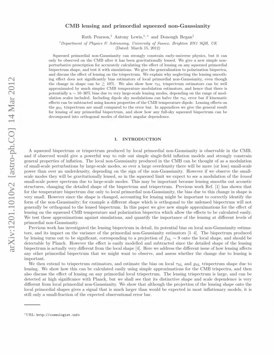
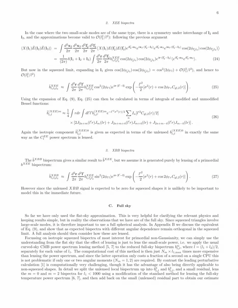
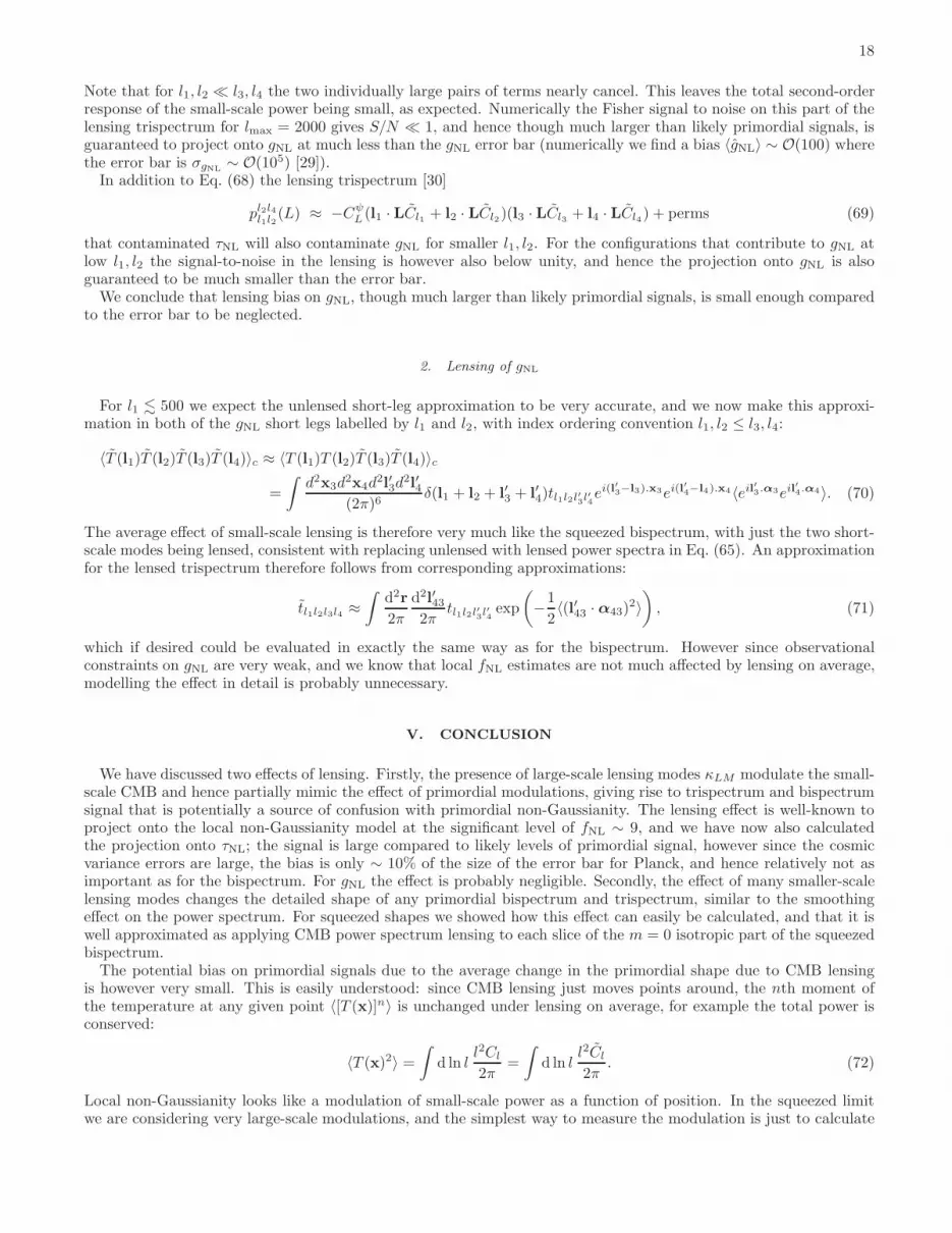
FIG. 1: The temperature CMB bispectrum from local non-Gaussianity (fNL = 1) with l1 = 30 (left) and l1 = 275 (right),projected into the isotropic component (solid lines), m = 2 quadrupole (green) and m = 4 (cyan) octopole parts. Thick linesare lensed using the approximation described in the text, thin lines show the unlensed bispectrum. The anisotropic componentsare small on super-horizon scales, and on smaller scales are relatively smooth so lensing has little effect. The definition of theangular components on the full sky is given in Appendix B.
where in the second line we expanded in k1/k for a scale-invariant spectrum, φ is the angle between the long andthe short-scale modes, and k ≡ (k3 − k2)/2. Thus in the squeezed limit there is no m dependence as expected, withleading corrections of O((k1/k)2) coming from the effect of gradients in the modulation.
Evolution until last scattering will modify this for observations of the CMB. However for l1 corresponding to scalesthat are super-horizon at recombination (l1 ≪ 100), the corresponding perturbation can be taken to be constantacross the last-scattering surface. The small-scale temperature is then modulated by 1 + (6fNL/5)ζ∗ (see moredetailed discussion below in Sec. IV A 1), and hence the local model bispectrum is
〈T (l1)T (l2)T (l3)〉 ≈ CTζ∗l1
⟨
δ
δζ∗(l1)∗(T (l2)T (l3))
⟩
(15)
=1
2πδ(l1 + l2 + l3)
6
5fNLC
Tζ∗l1
(Cl2 + Cl3), (16)
where ζ∗ is the primordial curvature perturbation at last scattering, ζ∗(n) = ζ(n, r∗) and r∗ is the distance to last-scattering1. We can see immediately that on the lensed sky, where the lenses are taken to be uncorrelated to theζ∗, the same result is obtained simply replacing Cl with the lensed Cl, and hence it should be no surprise that localbispectrum lensing is well modelled by power spectrum lensing. (Note that this low l1 limit is particularly interestingbecause non-linear evolution effects are under control analytically and known to be small [10].)
When l1 is larger the situation is more complicated since the modulation can no longer be approximated as beingconstant through last scattering. However the local bispectrum shape is still squeezed, so we can expect that our fullresult of Eq. (11) will accurately describe the effect of lensing where only the lowest angular bispectrum moments arerequired. Numerically, using the fully-sky analogue of the angular decomposition described in the appendix, we findthat the full sky temperature local bispectrum (calculated with camb) projected into only its isotropic part is ∼ 96%correlated to the full result (lmax = 2000, no noise), and 99% correlated if both the m = 0 and m = 2 (isotropic andquadrupolar) moments are retained. The quadrupolar moments are more important for larger (sub-horizon) l1 & 200.This is because the triangles with a given l have small-scale modes with transfer functions involving l2 and l3 that
1 Note that CTζ∗l
= βl(r∗) with βl(r) defined in Eq. (C2)

5
vary by ±l1/2 depending on φ, the angle between l1 and l; for l1 comparable to or larger than the separation of theacoustic peaks there is a significant variation in these transfer functions, giving a significant m 6= 0 component to thesqueezed CMB bispectrum for larger l1. See Fig. 1.
The unlensed short-leg approximation is expected to be quite accurate since almost all the signal to noise inlocal non-Gaussianity is at l1 . 500 for Planck sensitivity, where lensing effects are still small. We check theseapproximations numerically below by comparison with full-sky simulations.
B. Polarization
To consider polarization bispectra in the flat-sky approximation we need the lensed E and B modes given by thepolarization analogue of Eq. (2). Taking the unlensed B modes to be zero, it follows from the definitions given in [5]that:
E(l) =
∫
d2x
2π
d2l′
2πE(l′)eil
′·αeix(l′−l) cos 2φl′l (17)
B(l) =
∫
d2x
2π
d2l′
2πE(l′)eil
′·αeix(l′−l) sin 2φl′l , (18)
and φl′l is the angle between l′ and l. We can then use the lensed E and B modes to calculate the polarization
bispectra combinations in the unlensed short-leg approximation as before:
〈X(l1)Y (l2)Z(l3)〉 ≈ 〈X(l1)Y (l2)Z(l3)〉 =1
2πbXY Zl1l2l3δ(l1 + l2 + l3), (19)
where X , Y and Z can be any of T , E and B. For parity invariance fields bTEB = bEEB = 0.
1. XTE bispectra
Following the same steps as for the temperature case, the first combination gives
〈X(l1)T (l2)E(l3)〉 =
∫
d2x2
2π
d2x3
2π
d2l′22π
d2l′32π
〈X(l1)T (l′2)E(l′3)e−il2·x2eil′
2·(x2+α2)eil
′
3·α3eix3·(l
′
3−l3) cos(2φl′
3l3)〉. (20)
Keeping terms where α is uncorrelated to T and E, and writing the expectation value as a function of r ≡ x2 − x3
we have
〈X(l1)T (l2)E(l3)〉 =1
(2π)δ(l1 + l2 + l3)
∫
d2r
2π
d2l′22π
bXTEl1l′2l′
3
cos(2φl′3l3)eir·(l
′
2−l2)〈eil
′
2·α2eil
′
3·α3〉 (21)
where l3′ = −l1 − l′2. In the squeezed limit, expanding around l1 gives cos(2φl′
3l3) ≈ cos(2φl′l) + O(l1/l). Hence
neglecting non-Gaussianity of lensing potentials and very small terms for squeezed shapes we have
bXTEl1l2l3 ≈
∫
d2r
2π
d2l′
2πbXTEl1l′2l
′
3
cos(2φl′l)eir·(l′−l) exp
(
−l′2
2[σ2(r) + cos 2φl′rCgl,2(r)]
)
. (22)
Using the expansion of Eq. (9), the angular integrals can be done as in the temperature case, giving a result in termsof modified and unmodified Bessel functions:
b(XTE)ml1l
≈1
2
∫
rdr
∫
dl′l′b(XTE)ml1l′
e−l′2σ2(r)/2
∑
n
In[l′2Cgl,2(r)/2]
× [J2n+m+2(l′r)Jm+2(lr) + J2n+m−2(l′r)Jm−2(lr)] .
(23)
For the isotropic component b(XTE)0l1l
the two terms give equal contributions, and the result is then mathematically
the same as the result of the lensed CTEl power spectrum in terms of the unlensed spectrum (see e.g. Ref. [5]). Notehowever that in general m does not have to be even in the case of the XTE bispectrum, since there is no symmetrybetween the two small-scale modes. Nonetheless we can expect the main lensing effect to be described in terms of themonopole component, at least for low l1.
6
2. XEE bispectra
In the case where the two small-scale modes are of the same type, there is a symmetry under interchange of l2 andl3, and the approximations become valid to O(l21/l
2): following the previous argument
〈X(l1)E(l2)E(l3)〉 =
∫
d2x2
2π
d2x3
2π
d2l′22π
d2l′32π
⟨
X(l1)E(l′2)E(l′3)eil′
2·α2eix2·(l
′
2−l2)eil
′
3·α3eix3·(l
′
3−l3) cos(2φl′
3l3) cos(2φl′
2l2)⟩
=1
(2π)δ(l1 + l2 + l3)
∫
d2r
2π
d2l′22π
bXEEl1l′2l′
3
cos(2φl′3l3) cos(2φl′
2l2)eir·(l
′
2−l2)〈eil
′
2·α2eil
′
3·α3〉. (24)
But now in the squeezed limit, expanding in l1 gives cos(2φl′3l3) cos(2φl′
2l2) = cos2(2φl′l) + O(l21/l
2), and hence to
O(l21/l2)
bXEEl1l2l3 ≈
∫
d2r
2π
d2l′
2πbXEEl1l′2l
′
3
cos2(2φl′l)eir·(l′−l) exp
(
−l′2
2[σ2(r) + cos 2φl′rCgl,2(r)]
)
. (25)
Using the expansion of Eq. (9), Eq. (25) can then be calculated in terms of integrals of modified and unmodifiedBessel functions:
b(XEE)ml1l
≈1
4
∫
rdr
∫
dl′l′b(XEE)ml1l′
e−l′2σ2(r)/2
∑
n
In[l′2Cgl,2(r)/2]
× [2J2n+m(l′r)Jm(lr) + J2n+m+4(l′r)Jm+4(lr) + J2n+m−4(l′r)Jm−4(lr)] .
(26)
Again the isotropic component b(XEE)0l1l
is given as expected in terms of the unlensed b(XEE)0l1l
in exactly the same
way as the CEEl power spectrum is lensed.
3. XBB bispectra
The bXBB bispectrum gives a similar result to bXEE, but we assume it is generated purely by lensing of a primordialbXEE bispectrum:
bXBBl1l2l3 ≈
∫
d2r
2π
d2l′
2πbXEEl1l′2l
′
3
sin2(2φl′l)eir·(l′−l) exp
(
−l′2
2[σ2(r) + cos 2φl′rCgl,2(r)]
)
. (27)
However since the unlensed XBB signal is expected to be zero for squeezed shapes it is unlikely to be important tomodel this in the immediate future.
C. Full sky
So far we have only used the flat-sky approximation. This is very helpful for clarifying the relevant physics andkeeping results simple, but in reality the observations that we have are of the full sky. Since squeezed triangles involvelarge-scale modes, it is therefore important to use a full spherical analysis. In Appendix B we discuss the equivalentof Eq. (9), and show that as expected bispectra with different angular dependence remain orthogonal in the squeezedlimit. A full analysis should then consider how these are lensed.
Focussing on isotropic squeezed bispectra of most interest for primordial non-Gaussianity, we can simply use theunderstanding from the flat sky that the effect of lensing is just to lens the small-scale power, i.e. we apply the usualcurved-sky CMB power spectrum lensing method [5, 7] to the reduced full-sky bispectrum bml1l, where l = (l1 + l2)/2,separately for each value of l1. The computational cost of this method is then just Nm× l1,max times more expensivethan lensing the power spectrum, and since the latter operation only costs a fraction of a second on a single CPU thisis not problematic if only one or two angular moments (Nm = 1, 2) are required. By contrast the leading perturbativecalculation [1] is computationally very challenging, though it has the advantage of also being directly applicable tonon-squeezed shapes. In detail we split the unlensed local bispectrum up into b0l1l and b2l1l, and a small residual, lensthe m = 0 and m = 2 bispectra for l1 < 1000 using a modification of the standard method for lensing the full-skytemperature power spectrum [6, 7], and then add back on the small (unlensed) residual part to obtain our estimate
7
of the full lensed bispectrum. Our approximations are not valid for l1 ≫ 500, and the high l1 angular momentsbecome expensive to calculate, however most of the signal is at lower l1, so we only apply the lensing for l1 < 1000and approximate the (very small) contributions from higher l1 as being unlensed. It turns out that the m = 2 part ofthe bispectrum is rather smooth and not effected much by lensing, so lensing only the m = 0 component is usuallysufficient (Fig. 1).
Using our simple prescription for lensing the local non-Gaussianity we can then easily calculate various useful resultsto quantify the importance of lensing. Consider first noise-free temperature data to lmax = 2000. We find that thelensed local bispectrum is correlated at the > 0.999 level with the unlensed bispectrum, with the correction δb tothe bispectrum due to lensing only biasing estimators based on the unlensed shape by ∼ 0.007fNL (Ref. [1] havepreviously shown the bias is very small). This confirms that the correction due to lensing is almost orthogonal to theoriginal shape, which should not be surprising since lensing preserves total power (see discussion below). The changein shape due to lensing δb is detectable at one sigma for fNL ∼ 93. Including polarization data δb would be detectablefrom lensing of the isotropic component alone for fNL ∼ 22, but the bias remains small, ∼ 0.01fNL. For Planck noisethe current fNL limit is enough to rule out any chance of detecting the effect of lensing and we confirm the bias isnegligible.
III. COMPARISON WITH SIMULATIONS
To test our new approximation we compared it with simulations. We generated 480 full-sky Healpix [11] maps atlmax = 2500, nside = 2048 with fNL = 100 following the method of Ref. [1]. The unlensed input power spectra weretaken from camb [12]. The lensing potential power spectrum was then used to simulate uncorrelated lensing deflectionangle maps, and the unlensed maps were then lensed using LensPix [13, 14]. An estimator for the bispectrum in eachfull-sky noise-free realization is
Bijkl1l2l3 =∑
m1,m2,m3
(
l1 l2 l3m1 m2 m3
)
ail1m1ajl2m2
akl3m3, (28)
where i labels T , E or B, and we can relate to the reduced bispectrum bl1l2l3 defined using:
Bl1l2l3 =
√
(2l1 + 1)(2l2 + 1)(2l3 + 1)
4π
(
l1 l2 l30 0 0
)
bl1l2l3 . (29)
To reduce the variance and therefore the number of simulations needed to average over, we follow Ref. [1] by subtractinga term that averages to give zero bispectrum, but removes much of the realization-dependent variance. We also tookadvantage of symmetries to reduce the number of sums, using:
B′l1l2l3 =
l2∑
m2=0
l3∑
m3=−l3
(2 − δ0m2)
(
l1 l2 l3m1 m2 m3
)
ℜ [al1m1al2m2
al3m3− al1m1
al2m2al3m3
] (30)
where m1 = −m2 −m3, and alm and alm are the lensed spherical harmonic coefficients from maps generated usingthe same random seeds but with fNL 6= 0 and fNL = 0 respectively. Since we were running multiple simulations,and computational cost is nearly dominated by calculation of the 3j symbol, for each set of l,m we calculated theslice contributions from as many simulations as we could hold in memory. To avoid confusion with a lensing-induced
bispectrum, the lensing potential is generated with CTψl = CEψl = 0, so that the subtracted term involving a giveszero bispectrum on average. To test our bispectrum estimation method we compared unlensed simulated bispectraslices to the theory unlensed reduced bispectra generated by camb, with good agreement.
As a first check on polarization bispectra, we used the publicly-available simulated non-Gaussian polarization mapsfrom Ref. [15], which have a maximum multipole of 1024.
1. Simulation results
For the pure temperature bispectrum bTTTl1l2l3simulations were run up to a maximum multipole of 2000. (Although the
full-sky Healpix [11] maps were lmax = 2500, the lensing process requires a few hundred more multipoles than the scaleyou want to resolve.) The first acoustic peak of the CMB temperature power spectrum at l ∼ 200 corresponds to thescale which has just had time to maximally compress or expand by the time of recombination. Therefore a bispectrumwith l1 = 10 corresponds to very large super-horizon modulations in the small-scale power; this modulation is roughly
8
0 200 400 600 800 1000 1200 1400 1600 1800 2000
−0.1
−0.05
0
0.05
0.1
0.15
l
∆b10
,l,l+
10
b10
,l,l+
10
simulationstheory
0 200 400 600 800 1000 1200 1400 1600 1800 2000
−0.1
−0.05
0
0.05
0.1
0.15
l
∆b10
,l,l
b10
,l,l
simulationstheory
FIG. 2: The fractional change due to lensing in the reduced bispectrum slices bTTT10,l,l+10 and bTTT
10,l,l. The red shows the simulated
result averaged over 480 realizations. The bTTT10,l,l slice is somewhat noisier than the bTTT
10,l,l+10 slice (see discussion in text). Theblack line is the theoretical approximation of this paper, which agrees well with the simulations to within sample variance.
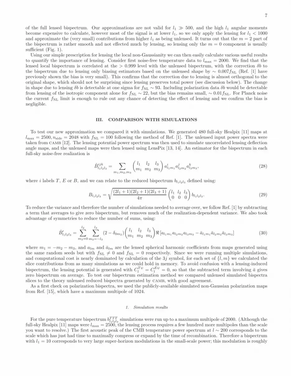
constant through the surface of last scattering (the approximation of Eq. 16). However a bispectrum with l1 = 200 willgive a modulation in small-scale power that varies significantly through the thickness of the last-scattering surface.We have tested our lensing approximation for both the case of constant and non-constant modulation by simulatingbispectra with both l1 = 10 and l1 = 200.
Because of the closure condition, a bispectrum with equal small scale modes (l2 = l3) looks like an isosceles triangle,where the large scale mode is roughly orthogonal to the short scale modes. For l3 = l1 + l2 (eg. b10,l,l+10), the closurecondition demands that the triangle you draw has zero area and all the modes are aligned (parallel). We test ifour lensing approximation holds for both orientations of modes by calculating bispectrum slices for both cases wherepossible. Since there is a significant quadrupolar m = 2 part of the bispectrum for l1 = 200, the slices for the differentmode orientations are quite different, and our simulations test that the decomposition of the bispectrum into modes,and lensing just the monopole part, works consistently. For l1 = 10 the bispectrum is nearly isotropic, so the slicesare very similar.
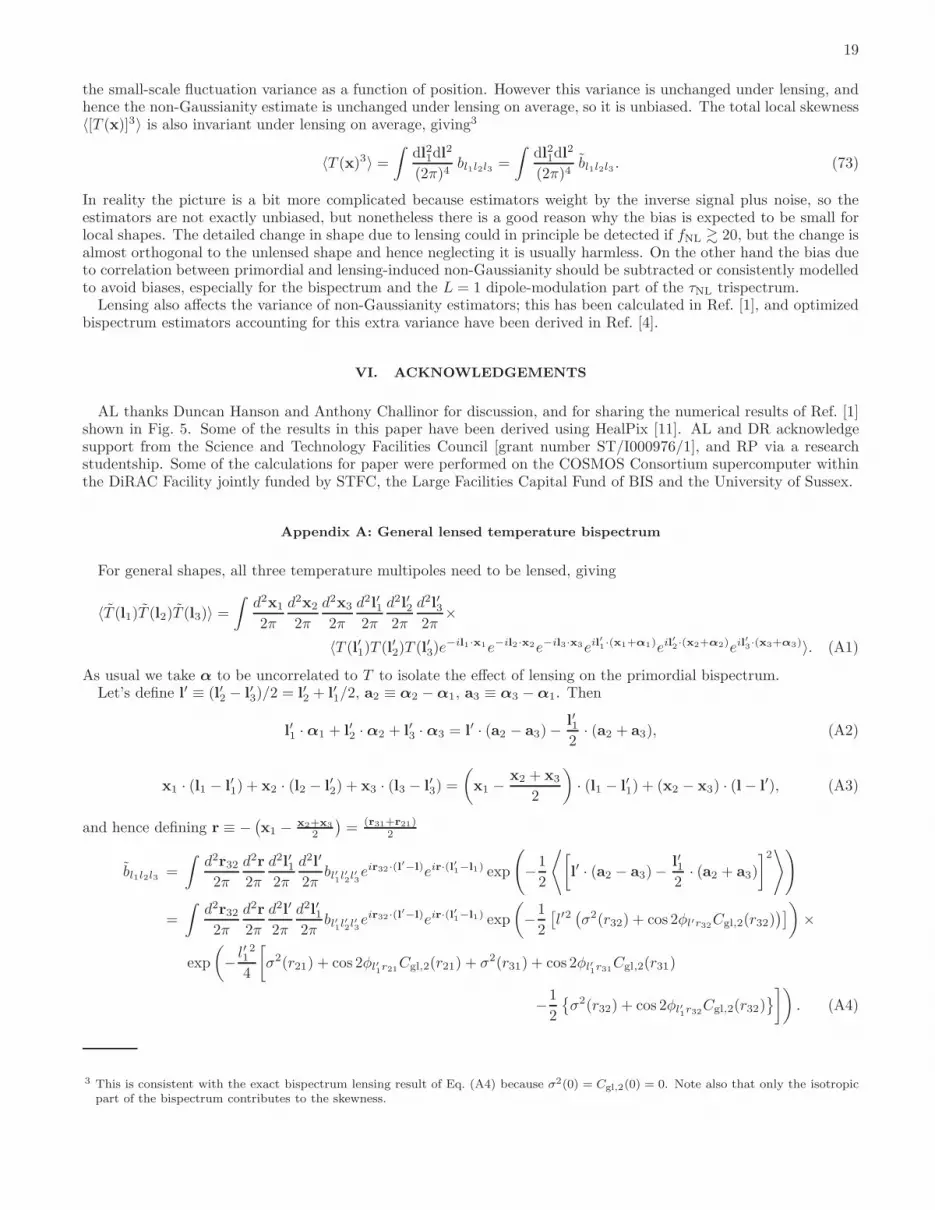
Fig. 2 shows the fractional change due to lensing for the reduced bispectrum slices bTTT10,l,l+10 and bTTT10,l,l, averaged over480 simulated maps. In these plots the simulated fractional change has been normalized to remove variance from thelarge scale l1 modes: since l1 = 10 is a super-horizon mode, its modulation is roughly constant across last scattering
and the bispectrum is roughly proportional to CTζ∗l1(Eq. 16). Both slices agree very well with the simulations, but
the bTTT10,l,l slice has more sampling noise as discussed further below.
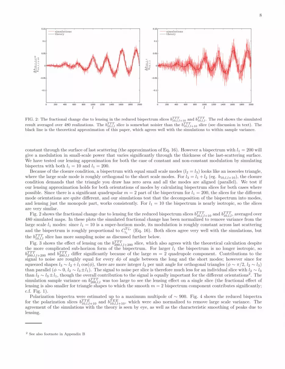
Fig. 3 shows the effect of lensing on the bTTT200,l,l+200 slice, which also agrees with the theoretical calculation despitethe more complicated sub-horizon form of the bispectrum. For larger l1 the bispectrum is no longer isotropic, sobTTT200,l,l+200 and bTTT200,l,l differ significantly because of the large m = 2 quadrupole component. Contributions to thesignal to noise are roughly equal for every dφ of angle between the long and the short modes; however since forsqueezed shapes l3 ∼ l2 + l1 cos(φ), there are more integer l3 per unit angle for orthogonal triangles (φ ∼ π/2, l2 ∼ l3)than parallel (φ ∼ 0, l2 ∼ l3± l1). The signal to noise per slice is therefore much less for an individual slice with l2 ∼ l3than l2 ∼ l3± l1, though the overall contribution to the signal is equally important for the different orientations2. Thesimulation sample variance on bTTT200,l,l was too large to see the lensing effect on a single slice (the fractional effect oflensing is also smaller for triangle shapes to which the smooth m = 2 bispectrum component contributes significantly;c.f. Fig. 1).
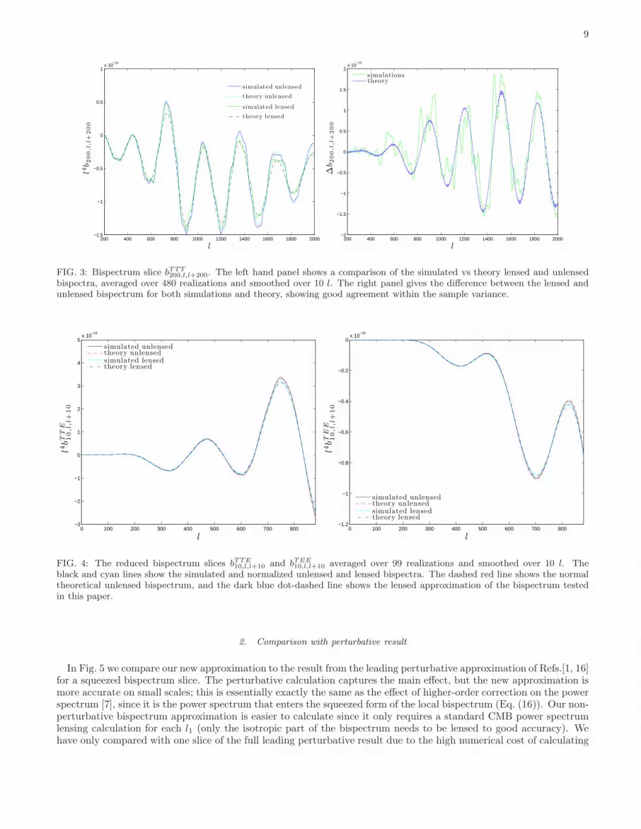
Polarization bispectra were estimated up to a maximum multipole of ∼ 900. Fig. 4 shows the reduced bispectrafor the polarization slices bTTE10,l,l+10 and bTEE10,l,l+10, which were also normalized to remove large scale variance. Theagreement of the simulations with the theory is seen by eye, as well as the characteristic smoothing of peaks due tolensing.
2 See also footnote in Appendix B
9
200 400 600 800 1000 1200 1400 1600 1800 2000−1.5
−1
−0.5
0
0.5
1x 10
−14
l
l4b 2
00
,l,l
+200
simulated unlensed
theory unlensed
simulated lensed
theory lensed
200 400 600 800 1000 1200 1400 1600 1800 2000−2
−1.5
−1
−0.5
0
0.5
1
1.5
2x 10
−15
l
∆b 2
00
,l,l
+200
simulationstheory
FIG. 3: Bispectrum slice bTTT200,l,l+200. The left hand panel shows a comparison of the simulated vs theory lensed and unlensed
bispectra, averaged over 480 realizations and smoothed over 10 l. The right panel gives the difference between the lensed andunlensed bispectrum for both simulations and theory, showing good agreement within the sample variance.
0 100 200 300 400 500 600 700 800−3
−2
−1
0
1
2
3
4
5x 10
−15
l
l4bT
TE
10
,l,l
+10
simulated unlensedtheory unlensedsimulated lensedtheory lensed
0 100 200 300 400 500 600 700 800−1.2
−1
−0.8
−0.6
−0.4
−0.2
0x 10
−15
l
l4bT
EE
10
,l,l
+10
simulated unlensedtheory unlensedsimulated lensedtheory lensed
FIG. 4: The reduced bispectrum slices bTTE10,l,l+10 and bTEE
10,l,l+10 averaged over 99 realizations and smoothed over 10 l. Theblack and cyan lines show the simulated and normalized unlensed and lensed bispectra. The dashed red line shows the normaltheoretical unlensed bispectrum, and the dark blue dot-dashed line shows the lensed approximation of the bispectrum testedin this paper.
2. Comparison with perturbative result
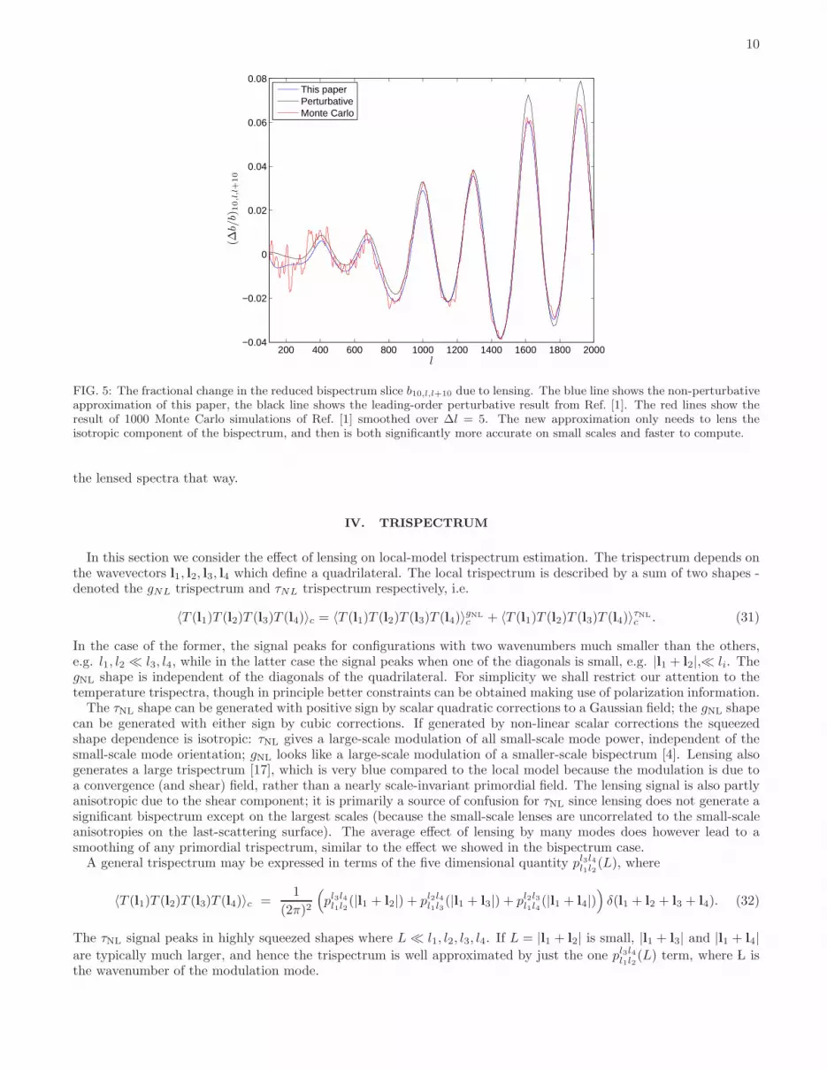
In Fig. 5 we compare our new approximation to the result from the leading perturbative approximation of Refs.[1, 16]for a squeezed bispectrum slice. The perturbative calculation captures the main effect, but the new approximation ismore accurate on small scales; this is essentially exactly the same as the effect of higher-order correction on the powerspectrum [7], since it is the power spectrum that enters the squeezed form of the local bispectrum (Eq. (16)). Our non-perturbative bispectrum approximation is easier to calculate since it only requires a standard CMB power spectrumlensing calculation for each l1 (only the isotropic part of the bispectrum needs to be lensed to good accuracy). Wehave only compared with one slice of the full leading perturbative result due to the high numerical cost of calculating
10
200 400 600 800 1000 1200 1400 1600 1800 2000−0.04
−0.02
0
0.02
0.04
0.06
0.08
l
(∆b/
b)10,l
,l+
10
This paperPerturbativeMonte Carlo
FIG. 5: The fractional change in the reduced bispectrum slice b10,l,l+10 due to lensing. The blue line shows the non-perturbativeapproximation of this paper, the black line shows the leading-order perturbative result from Ref. [1]. The red lines show theresult of 1000 Monte Carlo simulations of Ref. [1] smoothed over ∆l = 5. The new approximation only needs to lens theisotropic component of the bispectrum, and then is both significantly more accurate on small scales and faster to compute.
the lensed spectra that way.
IV. TRISPECTRUM
In this section we consider the effect of lensing on local-model trispectrum estimation. The trispectrum depends onthe wavevectors l1, l2, l3, l4 which define a quadrilateral. The local trispectrum is described by a sum of two shapes -denoted the gNL trispectrum and τNL trispectrum respectively, i.e.
〈T (l1)T (l2)T (l3)T (l4)〉c = 〈T (l1)T (l2)T (l3)T (l4)〉gNL
c + 〈T (l1)T (l2)T (l3)T (l4)〉τNL
c . (31)
In the case of the former, the signal peaks for configurations with two wavenumbers much smaller than the others,e.g. l1, l2 ≪ l3, l4, while in the latter case the signal peaks when one of the diagonals is small, e.g. |l1 + l2|,≪ li. ThegNL shape is independent of the diagonals of the quadrilateral. For simplicity we shall restrict our attention to thetemperature trispectra, though in principle better constraints can be obtained making use of polarization information.
The τNL shape can be generated with positive sign by scalar quadratic corrections to a Gaussian field; the gNL shapecan be generated with either sign by cubic corrections. If generated by non-linear scalar corrections the squeezedshape dependence is isotropic: τNL gives a large-scale modulation of all small-scale mode power, independent of thesmall-scale mode orientation; gNL looks like a large-scale modulation of a smaller-scale bispectrum [4]. Lensing alsogenerates a large trispectrum [17], which is very blue compared to the local model because the modulation is due toa convergence (and shear) field, rather than a nearly scale-invariant primordial field. The lensing signal is also partlyanisotropic due to the shear component; it is primarily a source of confusion for τNL since lensing does not generate asignificant bispectrum except on the largest scales (because the small-scale lenses are uncorrelated to the small-scaleanisotropies on the last-scattering surface). The average effect of lensing by many modes does however lead to asmoothing of any primordial trispectrum, similar to the effect we showed in the bispectrum case.
A general trispectrum may be expressed in terms of the five dimensional quantity pl3l4l1l2(L), where
〈T (l1)T (l2)T (l3)T (l4)〉c =1
(2π)2
(
pl3l4l1l2(|l1 + l2|) + pl2l4l1l3
(|l1 + l3|) + pl2l3l1l4(|l1 + l4|)
)
δ(l1 + l2 + l3 + l4). (32)
The τNL signal peaks in highly squeezed shapes where L ≪ l1, l2, l3, l4. If L = |l1 + l2| is small, |l1 + l3| and |l1 + l4|
are typically much larger, and hence the trispectrum is well approximated by just the one pl3l4l1l2(L) term, where L is
the wavenumber of the modulation mode.
11
The gNL shape is independent of the diagonals L of the quadrilaterals and may be expressed in terms of a fourdimensional quantity tl1l2l3l4 as
〈T (l1)T (l2)T (l3)T (l4)〉gNL
c =1
(2π)2tl1l2l3l4δ(l1 + l2 + l3 + l4). (33)
This equation may be written in the same form as Eq. (32) by identifying tl1l2l3l4 = pl3l4l1l2+ pl2l4l1l3
+ pl2l3l1l4with pl3l4l1l2
=
pl2l4l1l3= pl2l3l1l4
= tl1l2l3l4/3.
A. τNL Trispectrum
The τNL shape is most easily understood as measuring the power in large-scale modulations of small-scale power;we will show how τNL can easily be estimated very accurately (and nearly optimally) by making use of modulationestimators. These estimators reconstruct the modulation field on the CMB for each L ≡ l1 + l2, and the trispectrumis then measured by the modulation power spectrum for each value of L. Using this approach the bias due to lensingand the effect of lensing on the estimators is very easily calculated, and is essentially equivalent to using an accurateapproximation for the full trispectrum. For completeness we will then relate to a more direct full calculation. Sincethe τNL trispectrum involves nearly full-sky modulation scales, in this section we will do a spherical analysis.
1. Modulation estimators for τNL
A trispectrum of τNL form is generated by a primordial modulation of the fluctuations, where the modulationis not necessarily correlated to the large-scale Gaussian fields. For example if the small-scale Gaussian curvatureperturbation ζ0 is modulated by another field φ so that
ζ(x) = ζ0(x)[1 + φ(x)] (34)
where φ(x) is a small large-scale modulating field. The large-scale modes of φ can be measured by measuring themodulation it induces in the small-scale ζ power spectrum. If φ has a nearly scale-invariant spectrum, the nearly-white cosmic variance noise on the reconstruction dominates on small-scales, so only the very largest modes can bereconstructed (e.g. Ref. [18] find almost all the signal in the CMB is at modulation multipoles l < 10; see Fig. 6below). So a constraint on φ is going to be limited to only very large-scale variations, in which case the scale of thevariation is very large compared to the width of the last-scattering surface; i.e. in any particular direction a large-scale modulating field will modulate all perturbations through the last-scattering surface by approximately the sameamount. A large-scale power modulation therefore translates directly into a large-scale modulation of the small-scaleCMB temperature:
T (n) ≈ Tg(n)[1 + φ(n, r∗)], (35)
where Tg are the usual small-scale Gaussian CMB temperature anisotropies and r∗ is the radial distance to the last-scattering surface. This is not quite right for the large-scale temperature due to e.g. the ISW effect, but there arerelatively few large-scale modes and they have almost none of the signal to noise in the power modulation, so thiserror is harmless. But using this rather good approximation we can easily quantify the trispectrum as a function ofmodulation scale by using the power spectrum of the modulation,
τNL(L) ≡CφL
Cζ⋆L. (36)
Here were normalized conventionally relative to Cζ⋆L , the power spectrum of the primordial curvature perturbationat recombination (which we assume is known theoretically, but in practice cannot easily be measured at the relevantscale). For a scale-invariant primordial spectrum, Pζ = As the angular (not CMB!) power spectrum is simply
L(L+ 1)Cζ⋆L2π
= As. (37)
Note that τNL ∼ 500 corresponds to an O(10−3) modulation. In Appendix (C) we relate this to what you get applyingequivalent approximations to the full form of the τNL trispectrum.
12
In the simplest local non-Gaussianity model with ζ(x) = ζ0(x) + 35fNL(ζ0(x)2 −〈ζ20 〉), we can split ζ0 into long and
short modes ζl and ζs, then as far as observations of large-scale modulations are concerned we have
ζ = ζs(1 +3
5fNL[2ζl + ζs]) + ζl(1 +
3
5fNLζl) −
3
5fNL〈ζ
20 〉
≈ ζl + ζs
(
1 +6fNL
5ζl
)
. (38)
The modulation model for the small-scale modes is then φ = 6fNL
5 ζl, and hence τNL(L) = (6fNL/5)2 is scale-invariant.Any additional modulation field that is uncorrelated to ζ0 will not change the bispectrum but will increase τNL(L),hence in general τNL(L) ≥ (6fNL/5)2.
Regarding the modulation field as fixed, the small-scale fields being modulated are Gaussian so we can write downa Gaussian likelihood function. We can then try to find the modulation field that maximizes this Gaussian likelihood,giving an estimator for the modulation field. The technical details of how to do this are described in more detail inRef. [19], with the result that there is a quadratic maximum likelihood estimator for the large-scale modulation fieldφ given by:
φ = F−1[
hφ − 〈hφ〉
]
(39)
where h is a quadratic function of the filtered data that can be calculated quickly in real space:
hφLM =1
2
∑
l1m2,l2m2
δ〈Tl1m1T ∗l2m2
〉
δφ∗LM
∣
∣
∣
∣
∣
∣
φ=0
=
∫
dΩY ∗LM
[
∑
l1m1
Θl1m1Yl1m1
] [
∑
l2m2
Cl2Θl2m2Yl2m2
]
. (40)
Here Θ = cov−1T is the observed CMB sky after inverse-variance filtering (which accounts for sky cuts and inhomo-
geneous noise), and Cl2 is the lensed Cl (since the covariance in the lensed sky involves the lensed power spectra, andwe neglect the effect of lensing modes correlated to φLM ). The normalization F is given by the Fisher matrix. In thesimple full-sky case with isotropic noise this is
Flm,l′m′ = δll′δmm′
∑
l1,l2
(2l1 + 1)(2l2 + 1)
8π
(
l l1 l20 0 0
)2(Cl1 + Cl2)2
Ctotl1Ctotl2
, (41)
and the estimator noise is NL = F−1LL. Here Ctot
l1is the lensed spectrum plus any (isotropic) noise. For low L and
high lmax the reconstruction noise is very nearly constant (white, because each small patch of sky gives a nearly-uncorrelated but noisy estimate of the small-scale power). We can then define an estimator of the modulation powerspectrum
CφL =1
2L+ 1
∑
M
|φLM |2 −N(0)L , (42)
where N(0)L = 〈|φLM |2〉0 is a noise bias for zero signal (the same as NL in the full-sky case). Additional “N (1)”
(O(Cφ)) biases from cross-terms are expected to be small, and in any case vanish in the case of zero signal and hencewould not give a spurious detection. On the cut sky pseudo-Cl estimators can be used [19, 20].
For each value of the modulation scale L, Eq. (42) gives a separate estimator for τNL. In the ideal case we can
combine them by inverse variance weighting with var(CφL) = 2N2L/(2L+ 1), giving the combined estimator
τNL ≡
∑
L var[τNL(L)]−1τNL(L)∑
L var[τNL(L)]−1= σ2
τNL
∑
L
(2L+ 1)Cζ∗L2NL
CφL (43)
where (σ2τNL
)−1 =∑
L(2L+ 1)/(2NL[Cζ⋆L ]2). Using the approximations CζL ∝ (L(L+ 1))−1, and the constancy of thewhite reconstruction noise NL, we have
τNL ≈ L2min
∞∑
L=Lmin
2L+ 1
L2(L+ 1)2CφLCζ⋆L
. (44)
13
If there is a scale-invariant signal so CφL ∝ CζL, we see that as expected the contributions fall rapidly ∝ 1/L3, asexpected when measuring a scale-invariant signal that has large white noise. The total variance is
var(τNL) ≈2L2
minN2L
(2πAs)2. (45)
Note that if the L = 1 dipolar modulation is excluded so that Lmin = 2, the τNL variance becomes four times largerthan if the dipole is included. We have 95% of the signal at L ≤ 4, justifying the squeezed approximations used,and hence confirming that they should be good to percent-level accuracy. Assuming the only non-Gaussian signalis τNL, for a noise-free temperature-only experiment to lmax = 2000 Eq. (45) gives στNL
∼ 150 (in good agreementwith [18] given parameter dependence; note that errors in [20] are a factor of two larger because they exclude the
dipole); for Planck στNL∼ 300. Using numerical values for CζL gives somewhat more accurate results for non-scale
invariant spectra, with στNL=(∑
L var[τNL(L)]−1)−1/2
≈ 134 for noise-free data to lmax = 2000, and στNL∼ 200–300
for Planck depending on assumptions.The approximation here essentially re-writes the τNL estimators of Ref. [20] by analytically approximating the radial
integrals, resulting in the CMB temperature power anisotropy estimators of Ref. [19]. The approximation consists oftaking the recombination visibility as a delta-function compared to the modulation scale of interest, combined withneglect of small cross terms that complicate the relationship between the modulation power spectra and trispectrum(see Ref. [21, 22] for an extensive discussion in the context of CMB lensing where the latter corrections are moreimportant on small scales). In exchange for these approximations we find estimators that are simple to interpret, fastto evaluate, can incorporate full inverse-variance weighting for optimality with real data, and allow other complicatingeffects such as lensing to be easily understood and modelled.
The approximate estimator described here accounts for the average effect of small-scale lensing modes in a verysimple way, since the only effect is to change the map filter functions so that they involve lensed rather than unlensedpower spectra. This is consistent with the expression of the lensed trispectrum given in Appendix C, which onlyinvolves power spectra in an equivalent approximation: the large-scale primordial modulation modes cause a modu-lation in the fully non-linear observed small-scale power. The effect of the modulation on the lensing potential can beneglected since it only leads to an O(10−3) correction to the already-small lensing effect.
2. Lensing bias
The above analysis has assumed the only anisotropy was due to primordial modulation. There will also be lensinganisotropy due to large-scale lensing modes (and, for L = 1, Doppler modulation and angular abberation, as discussedfurther below). However as discussed in detail in Ref. [23] it is straightforward to account for multiple sources ofanisotropy if required, or suboptimally by including lensing in the simulations that are used to subtract noise biases.Here we simply estimate the impact of large-scale lensing modes on a τNL estimator: i.e. if we neglect lensing, atwhat level is the simplest τNL estimator biased?
Writing the quadratic estimator in harmonic space
hφlm =1
2
∑
l1,m1,l2,m2
√
(2l+ 1)(2l1 + 1)(2l2 + 1)
4π
(
l l1 l20 0 0
)(
l l1 l2m m1 m2
)
(Cl1 + Cl2)Θ∗l1m1
Θ∗l2m2
(46)
we can simply calculate the expectation due to other forms of anisotropy such as lensing. Averaging over small-scaleGaussian lensing and temperature modes (lm) 6= (l1m1) for fixed convergence κl1m1
we have [4, 24]
∑
m2m3
(
l1 l2 l3m1 m2 m3
)
〈Tl2m2Tl3m3
〉(lm) 6=(l1m1) ≈∑
m2m3
(
l1 l2 l3m1 m2 m3
)
⟨
δ
δκ∗l1m1
(
Tl2m2Tl3m3
)
⟩
κ∗l1m1
≈1
(2l1 + 1)
√
(2l1 + 1)(2l2 + 1)(2l3 + 1)
4π
(
l1 l2 l30 0 0
)
Kl1l2l3κ∗l1m1
, (47)
where we defined
Kl1l2l3 ≡ (Cl2 + Cl3) + (Cl2 − Cl3)
[
l2(l2 + 1) − l3(l3 + 1)
l1(l1 + 1)
]
. (48)
14
5 10 15 20 25 30 35 4010
−1
100
101
102
103
104
105
L
Contribution to S/N for τ
NL
Lensing bias contribution∝ 1/L3
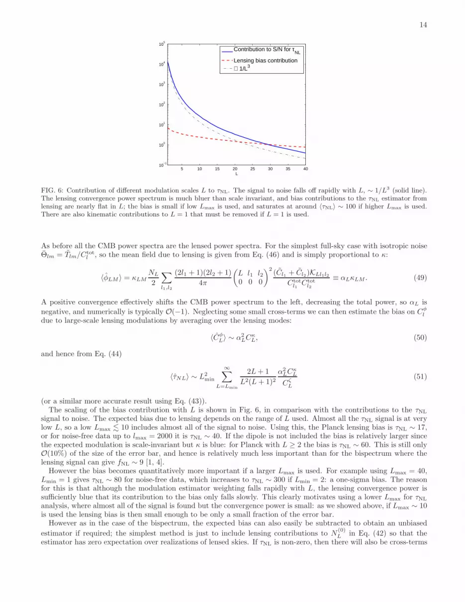
FIG. 6: Contribution of different modulation scales L to τNL. The signal to noise falls off rapidly with L, ∼ 1/L3 (solid line).The lensing convergence power spectrum is much bluer than scale invariant, and bias contributions to the τNL estimator fromlensing are nearly flat in L; the bias is small if low Lmax is used, and saturates at around 〈τNL〉 ∼ 100 if higher Lmax is used.There are also kinematic contributions to L = 1 that must be removed if L = 1 is used.
As before all the CMB power spectra are the lensed power spectra. For the simplest full-sky case with isotropic noiseΘlm = Tlm/C
totl , so the mean field due to lensing is given from Eq. (46) and is simply proportional to κ:
〈φLM 〉 = κLMNL2
∑
l1,l2
(2l1 + 1)(2l2 + 1)
4π
(
L l1 l20 0 0
)2(Cl1 + Cl2)KLl1l2
Ctotl1Ctotl2
≡ αLκLM . (49)
A positive convergence effectively shifts the CMB power spectrum to the left, decreasing the total power, so αL is
negative, and numerically is typically O(−1). Neglecting some small cross-terms we can then estimate the bias on Cφldue to large-scale lensing modulations by averaging over the lensing modes:
〈CφL〉 ∼ α2LC
κL, (50)
and hence from Eq. (44)
〈τNL〉 ∼ L2min
∞∑
L=Lmin
2L+ 1
L2(L + 1)2α2LC
κL
CζL(51)
(or a similar more accurate result using Eq. (43)).The scaling of the bias contribution with L is shown in Fig. 6, in comparison with the contributions to the τNL
signal to noise. The expected bias due to lensing depends on the range of L used. Almost all the τNL signal is at verylow L, so a low Lmax . 10 includes almost all of the signal to noise. Using this, the Planck lensing bias is τNL ∼ 17,or for noise-free data up to lmax = 2000 it is τNL ∼ 40. If the dipole is not included the bias is relatively larger sincethe expected modulation is scale-invariant but κ is blue: for Planck with L ≥ 2 the bias is τNL ∼ 60. This is still onlyO(10%) of the size of the error bar, and hence is relatively much less important than for the bispectrum where thelensing signal can give fNL ∼ 9 [1, 4].
However the bias becomes quantitatively more important if a larger Lmax is used. For example using Lmax = 40,Lmin = 1 gives τNL ∼ 80 for noise-free data, which increases to τNL ∼ 300 if Lmin = 2: a one-sigma bias. The reasonfor this is that although the modulation estimator weighting falls rapidly with L, the lensing convergence power issufficiently blue that its contribution to the bias only falls slowly. This clearly motivates using a lower Lmax for τNL
analysis, where almost all of the signal is found but the convergence power is small: as we showed above, if Lmax ∼ 10is used the lensing bias is then small enough to be only a small fraction of the error bar.
However as in the case of the bispectrum, the expected bias can also easily be subtracted to obtain an unbiased
estimator if required; the simplest method is just to include lensing contributions to N(0)L in Eq. (42) so that the
estimator has zero expectation over realizations of lensed skies. If τNL is non-zero, then there will also be cross-terms
15
from universe-sized modes generating correlated low multipole signals in both the lensing potential and the primordialmodulation.
The Doppler dipole due to the earth’s motion is ∼ 10−3, and induces aberration and CMB temperature modulationat this level [25–27]. If data are used to constrain τNL using the dipole modulation (which shrinks the error barby a factor of two relative to starting at L = 2), the dipole-induced signal must be subtracted since its modulationreconstruction has signal-to-noise larger than one at Planck resolution. However we know the direction of the kinematicdipole in the CMB temperature, and hence both the magnitude and direction of the modulation that is expected; itcan therefore be directly subtracted from the reconstructed dipole modulation field, and as long as this can be doneto O(10%) accuracy it should not be an obstacle to also detecting a primordial τNL that is detectable in the absenceof kinematic effects. If the dipole is not used, the dominant primordial signal is then in the quadrupole, which maybe susceptible to observational artefacts due to the quadrupolar dependence of Planck scan strategy, for example dueto gain variations. Even in the absence of unexpectedly large primordial signals, tests for modulations can be a usefulprobe of instrumental systematics.
3. Lensing bias from simulations and full τNL estimators
To check consistency of the various approximations, we implement the trispectrum estimator as described in Ref. [28]and estimate the lensing bias from simulations. The estimator was tested using 300 Gaussian maps, which were thenlensed using LensPix as before.
The averaged full-sky estimator with isotropic noise is given by
〈E〉 =1
8F
∑
limi
∑
LM
pl1l2l3l4(L)(−1)MGl1l2Lm1m2−M
Gl3l4Lm3m4M
Ctotl1Ctotl2Ctotl3Ctotl4
[
〈al1m1al2m2
al3m3al4m4
〉 − 〈al1m1al2m2
〉〈al3m3al4m4
〉
− 〈al1m1al4m4
〉〈al2m2al3m3
〉 − 〈al1m1al3m3
〉〈al2m2al4m4
〉
]
, (52)
where the angular brackets 〈. . . 〉 refer to averaging over the simulations and the Gaunt integral is given by Gl1l2l3m1m2m3=
∫
dnYl1m1Yl2m2
Yl3m3. The denominator is given by the Fisher matrix,
F =1
8
∑
liL
P l1l2l3l4(L)
Ctotl1Ctotl2Ctotl3Ctotl4
(P l1l2l3l4(L)
2L+ 1+∑
L′
(−1)l2+l3
l1 l2 Ll4 l3 L′
P l1l3l2l4(L′) +
∑
L′
(−1)L+L′
l1 l2 Ll3 l4 L′
P l1l4l3l2(L′)
)
,
(53)
where . . . refer to the Wigner 6j symbols, and P l1l2l3l4(L) = pl1l2l3l4
(L)hl1l2Lhl3l4L, with hl1l2L ≡√
(2l1+1)(2l2+1)(2L+1)4π
(
l1 l2 L0 0 0
)
. In the case of the local model τNL trispectrum (given by (C1)), the squeezed shape
dependence means that only P l1l2l3l4(L) contributes significantly, and F may be efficiently and accurately calculated
using [18],
F =1
8
∑
liL
pl1l2l3l4(L)2h2l1l2Lh
2l3l4L
Ctotl1Ctotl2Ctotl3Ctotl4
. (54)
The optimal signal to noise of the trispectrum is given by F , and the corresponding variance of τNL is given by itsinverse. For lmax = 2000 the error bar is given by σ(τNL) = 129, where the sum over L has been calculated for1 ≤ L ≤ 100. We checked that the sum has converged to within ∼ 2% of its final value by L = 5 and to within ∼ 0.5%
by L = 10. Furthermore, the replacement of FL(r1, r2) by FL(r∗, r∗) = Cζ∗L , as described in Appendix C results inlittle loss of accuracy, with the variance in τNL agreeing with the previous estimate to within O(1%). Calculating thefull trispectrum of Eq. (C1) however involves doing radial integrals, and the numerical error involved can be largerthan the theoretical approximations made in the previous sections. The direct calculation of σ(τNL) = 129 agreesquite well with the previous modulation-estimator value of σ(τNL) = 134, with a small portion of the difference beingmade up by O(1%) theoretical approximations, and few percent numerical errors.
Using FL(r1, r2) ∼ FL(r∗, r∗), the estimator for the amplitude of the local τNL model reads
τNL =1
2F
∑
L
FL(r∗, r∗)[
∑
M
|(A ∗B)LM |2 −∑
l1l2
h2l1l2L2Ctot
l1Ctotl2
AB(l1, l2)2]
, (55)
16
where
(A ∗B)LM =
∫
dnY ∗LM (n)
∫
drr2A(r, n)B(r, n), (56)
A(r, n) =∑
l1m1
αl1(r)al1m1Yl1m1
(n)
Ctotl1
, (57)
B(r, n) =∑
l1m1
βl1(r)al1m1Yl1m1
(n)
Ctotl1
, (58)
AB(l1, l2) =
∫
drr2 (αl1(r)βl2 (r) + αl2(r)βl1(r)) , (59)
and where Ctotl1
= Cl1 for unlensed Gaussian maps, but is replaced by the lensed angular power spectrum for thelensed Gaussian maps (plus noise if applicable). Using the further accurate approximation of Eq. (C5), Eq. (55) isconsistent with the previous modulation estimator of Eq. (43) for the low L of interest. In fact we have verified thatuse of this approximation in the estimator recovers the same variance and bias to O(1 − 2%).
The variance and mean of the estimator has been calculated over 300 Gaussian simulations giving a sampling biasof 3, and a one sigma error of 130. This error bar agrees quite well with the expected variance of 129.
Applying the estimator up to Lmax = 10 to the lensed maps reveals a bias of 49 and a slightly enlarged varianceof 141. Hence, application of the equation (52) verifies that large-scale lensing modes may introduce a small bias onτNL estimators of O(30%) the size of the error bar for noise-free data out to lmax = 2000. Extending the summationto Lmax = 100 increases the bias to 107, confirming the expectation that the bias would become quantitatively largerdue to the blue spectrum of the lensing convergence. A realistic analysis on the lensed sky can restrict to a muchlower value of Lmax to keep the bias small, with very little loss of τNL signal.
We conclude that the modulation estimator is fully consistent with a more brute-force τNL estimator, and in factthat the rather accurate theoretical approximations (. 1%) involved are likely to be more accurate than numericalerrors involved in the full estimator (which involves performing numerical radial integrals). Both are accurate towithin a small fraction of the error bar, but the modulation estimator is significantly faster to calculate and makes itmuch simpler to calculate complications such as lensing bias.
4. Lensing of the τNL trispectrum
We have shown how to easily account for the main effects of lensing when estimating τNL, and quantified the biasdue to overlap between the τNL and lensing trispectrum shapes. Here we briefly consider how this is consistent withthe direct result for lensing of a primordial τNL trispectrum.
The lensed τNL trispectrum is defined by
〈T (l1)T (l2)T (l3)T (l4)〉c =1
(2π)2
(
pl3l4l1l2(|l1 + l2|) + pl2l4l1l3
(|l1 + l3|) + pl2l3l1l4(|l1 + l4|)
)
δ(l1 + l2 + l3 + l4). (60)
In terms of the unlensed trispectrum we have
〈T (l1)T (l2)T (l3)T (l4)〉c =
∫
Π4i=1
(
d2xid2l′i
(2π)2
)
δ(∑
i
l′i)
1
(2π)2
[
pl′3l′4
l′1l′2
(|l′1 + l′2|) + (2 perms)
]
× ei(l′
1−l1).x1ei(l
′
2−l2).x2ei(l
′
3−l3).x3ei(l
′
4−l4).x4〈eil
′
1.α1eil
′
2.α2eil
′
3.α3eil
′
4.α4〉. (61)
Using statistical homogeneity we may assume that the expectation value is independent of∑
i xi. Defining l43 ≡(l4 − l3)/2, l21 ≡ (l2 − l1)/2, L ≡ l1 + l2, r ≡ (x1 + x2 − x3 − x4)/2 this allows us to write
pl3l4l1l2(L) =
∫
d2r12d2r34d
2rd2l′21d
2l′43d
2L′
(2π)6pl′3l′4
l′1l′2
(L′)eir21.(l′
21−l21)eir43.(l
′
43−l43)eir.(L
′−L)
× 〈eil′
21.α21eil
′
43.α43ei
12L
′·(α1+α2−α3−α4)〉, (62)
where we assumed a squeezed shape, L′, L≪ li, l′i and so only kept pl3l4l1l2
(L). Also for squeezed shapes we can neglect
the L′ term in the exponential (as for the bispectrum), and we have
〈eil′
21.α21eil
′
43.α43〉 = exp
(
−1
2〈(l′21.α21)2〉
)
exp(
−1
2〈(l′43.α43)2〉
)
exp(
− 〈(l′21.α21)(l′43.α43)〉)
. (63)
17
The first two terms are exactly the terms that appear in bispectrum lensing (c.f. Eq. (7)), and hence are wellapproximated by power spectrum lensing of the small-scale power at wavenumbers l21 and l43. The last term is anadditional effect coming from the fact that the lenses acting on different pairs of small-scale modes are correlated (allsmall-scale modes see the same lensing potential realization). It depends on r, and hence in principle gives rise tocouplings between L 6= L
′; however we are interested in very low L, corresponding to a scale much larger than thearcminute lensing deflections, so we can expect L ≈ L
′ to a good approximation for all trispectrum components ofinterest. This is consistent because the difference in deflection angles at x1,x2 and x3,x4 will only be very weaklycorrelated for large r separation of the pairs of points, so the third term in Eq. (63) can be neglected.
This allows us to find the following estimate for the lensed τNL trispectrum,
pl3l4l1l2(L) ≈
∫
d2r21d2r43d
2l′21d
2l′43
(2π)4pl′3l′4
l′1l′2
(L)eir21.(l′
21−l21)eir43.(l
′
43−l43)
× exp(
−1
2〈(l′21.α21)2〉
)
exp(
−1
2〈(l′43.α43)2〉
)
, (64)
where the expectation values can be calculated exactly as for power spectrum and bispectrum lensing. Since thetrispectrum is well approximated as involving only the CMB power spectrum on the small-scale modes (see Ap-pendix C), this is consistent with lensing simply replacing the unlensed power spectra by the lensed spectra.
B. gNL trispectrum
The gNL trispectrum can be generated by local cubic corrections to a Gaussian field. It essentially measures thecorrelation of a small-scale local fNL with the large-scale field. Since local fNL itself has all the signal in squeezedshapes, this means that the signal in gNL is dominated by shapes with l1, l2 ≪ l3, l4, though unlike in the τNL
trispectrum the signal is not all in l1 ∼ 1. For simplicity we will use the flat-sky approximation here.We can approximate the primordial gNL signal by taking the large-scale curvature modes with wavenumbers l1 and
l2 to be constant through last scattering. For a primordial curvature perturbation ζ = ζ0 + gNLζ30 the contribution to
the trispectrum in this regime is then determined by
〈T (l1)T (l2)T (l3)T (l4)〉c ≈ CTζ∗l1CTζ∗l2
⟨
δ
δζ∗(l2)∗δ
δζ∗(l1)∗(T (l3)T (l4))
⟩
≈6
(2π)2gNLC
Tζ∗l1
CTζ∗l2(Cl3 + Cl4)δ(l1 + l2 + l3 + l4), (65)
where ζ∗ is the primordial curvature perturbation at last scattering. This is a good approximation for l1, l2 ≪ 100,but breaks down for the contributions where l2 & 100 where the finite thickness of last-scattering becomes important.However it is sufficient for ballpark estimates of the signal to noise and bias.
1. Lensing bias
With l1, l2 ≤ l3, l4, the gNL-type trispectrum due to lensing is of the form
〈T (l1)T (l2)T (l3)T (l4)〉c ≈ CTψl1 CTψl2
⟨
δ
δψ(l1)∗δψ(l2)∗
(
T (l3)T (l4))
⟩
, (66)
where ψ is the lensing potential that gives the deflection angle α = ∇ψ. Using
δ
δψ(l)∗ei·l
′·(x+α) =1
2πl · l′eil
′·(x+α)e−il·x (67)
and evaluating to leading order we have
〈T (l1)T (l2)T (l3)T (l4)〉c ≈1
(2π)2CTψl1 CTψl2
[
l1 · l4 l2 · l4Cl4 + l1 · l3 l2 · l3Cl3
− l1 · (l1 + l3)l2 · (l1 + l3)C|l1+l3| − l1 · (l1 + l4)l2 · (l1 + l4)C|l1+l4|
]
δ(l1 + l2 + l3 + l4). (68)
18
Note that for l1, l2 ≪ l3, l4 the two individually large pairs of terms nearly cancel. This leaves the total second-orderresponse of the small-scale power being small, as expected. Numerically the Fisher signal to noise on this part of thelensing trispectrum for lmax = 2000 gives S/N ≪ 1, and hence though much larger than likely primordial signals, isguaranteed to project onto gNL at much less than the gNL error bar (numerically we find a bias 〈gNL〉 ∼ O(100) wherethe error bar is σgNL
∼ O(105) [29]).In addition to Eq. (68) the lensing trispectrum [30]
pl2l4l1l2(L) ≈ −CψL (l1 · LCl1 + l2 · LCl2)(l3 · LCl3 + l4 · LCl4) + perms (69)
that contaminated τNL will also contaminate gNL for smaller l1, l2. For the configurations that contribute to gNL atlow l1, l2 the signal-to-noise in the lensing is however also below unity, and hence the projection onto gNL is alsoguaranteed to be much smaller than the error bar.
We conclude that lensing bias on gNL, though much larger than likely primordial signals, is small enough comparedto the error bar to be neglected.
2. Lensing of gNL
For l1 . 500 we expect the unlensed short-leg approximation to be very accurate, and we now make this approxi-mation in both of the gNL short legs labelled by l1 and l2, with index ordering convention l1, l2 ≤ l3, l4:
〈T (l1)T (l2)T (l3)T (l4)〉c ≈ 〈T (l1)T (l2)T (l3)T (l4)〉c
=
∫
d2x3d2x4d
2l′3d
2l′4
(2π)6δ(l1 + l2 + l
′3 + l
′4)tl1l2l′3l′4e
i(l′3−l3).x3ei(l
′
4−l4).x4〈eil
′
3.α3eil
′
4.α4〉. (70)
The average effect of small-scale lensing is therefore very much like the squeezed bispectrum, with just the two short-scale modes being lensed, consistent with replacing unlensed with lensed power spectra in Eq. (65). An approximationfor the lensed trispectrum therefore follows from corresponding approximations:
tl1l2l3l4 ≈
∫
d2r
2π
d2l′43
2πtl1l2l′3l′4 exp
(
−1
2〈(l′43 · α43)2〉
)
, (71)
which if desired could be evaluated in exactly the same way as for the bispectrum. However since observationalconstraints on gNL are very weak, and we know that local fNL estimates are not much affected by lensing on average,modelling the effect in detail is probably unnecessary.
V. CONCLUSION
We have discussed two effects of lensing. Firstly, the presence of large-scale lensing modes κLM modulate the small-scale CMB and hence partially mimic the effect of primordial modulations, giving rise to trispectrum and bispectrumsignal that is potentially a source of confusion with primordial non-Gaussianity. The lensing effect is well-known toproject onto the local non-Gaussianity model at the significant level of fNL ∼ 9, and we have now also calculatedthe projection onto τNL; the signal is large compared to likely levels of primordial signal, however since the cosmicvariance errors are large, the bias is only ∼ 10% of the size of the error bar for Planck, and hence relatively not asimportant as for the bispectrum. For gNL the effect is probably negligible. Secondly, the effect of many smaller-scalelensing modes changes the detailed shape of any primordial bispectrum and trispectrum, similar to the smoothingeffect on the power spectrum. For squeezed shapes we showed how this effect can easily be calculated, and that it iswell approximated as applying CMB power spectrum lensing to each slice of the m = 0 isotropic part of the squeezedbispectrum.
The potential bias on primordial signals due to the average change in the primordial shape due to CMB lensingis however very small. This is easily understood: since CMB lensing just moves points around, the nth moment ofthe temperature at any given point 〈[T (x)]n〉 is unchanged under lensing on average, for example the total power isconserved:
〈T (x)2〉 =
∫
d ln ll2Cl2π
=
∫
d ln ll2Cl2π
. (72)
Local non-Gaussianity looks like a modulation of small-scale power as a function of position. In the squeezed limitwe are considering very large-scale modulations, and the simplest way to measure the modulation is just to calculate
19
the small-scale fluctuation variance as a function of position. However this variance is unchanged under lensing, andhence the non-Gaussianity estimate is unchanged under lensing on average, so it is unbiased. The total local skewness〈[T (x)]3〉 is also invariant under lensing on average, giving3
〈T (x)3〉 =
∫
dl21dl2
(2π)4bl1l2l3 =
∫
dl21dl2
(2π)4bl1l2l3 . (73)
In reality the picture is a bit more complicated because estimators weight by the inverse signal plus noise, so theestimators are not exactly unbiased, but nonetheless there is a good reason why the bias is expected to be small forlocal shapes. The detailed change in shape due to lensing could in principle be detected if fNL & 20, but the change isalmost orthogonal to the unlensed shape and hence neglecting it is usually harmless. On the other hand the bias dueto correlation between primordial and lensing-induced non-Gaussianity should be subtracted or consistently modelledto avoid biases, especially for the bispectrum and the L = 1 dipole-modulation part of the τNL trispectrum.
Lensing also affects the variance of non-Gaussianity estimators; this has been calculated in Ref. [1], and optimizedbispectrum estimators accounting for this extra variance have been derived in Ref. [4].
VI. ACKNOWLEDGEMENTS
AL thanks Duncan Hanson and Anthony Challinor for discussion, and for sharing the numerical results of Ref. [1]shown in Fig. 5. Some of the results in this paper have been derived using HealPix [11]. AL and DR acknowledgesupport from the Science and Technology Facilities Council [grant number ST/I000976/1], and RP via a researchstudentship. Some of the calculations for paper were performed on the COSMOS Consortium supercomputer withinthe DiRAC Facility jointly funded by STFC, the Large Facilities Capital Fund of BIS and the University of Sussex.
Appendix A: General lensed temperature bispectrum
For general shapes, all three temperature multipoles need to be lensed, giving
〈T (l1)T (l2)T (l3)〉 =
∫
d2x1
2π
d2x2
2π
d2x3
2π
d2l′12π
d2l′22π
d2l′32π
×
〈T (l′1)T (l′2)T (l′3)e−il1·x1e−il2·x2e−il3·x3eil
′
1·(x1+α1)eil
′
2·(x2+α2)eil
′
3·(x3+α3)〉. (A1)
As usual we take α to be uncorrelated to T to isolate the effect of lensing on the primordial bispectrum.Let’s define l
′ ≡ (l′2 − l′3)/2 = l
′2 + l
′1/2, a2 ≡ α2 −α1, a3 ≡ α3 −α1. Then
l′1 ·α1 + l
′2 ·α2 + l
′3 · α3 = l
′ · (a2 − a3) −l′1
2· (a2 + a3), (A2)
x1 · (l1 − l′1) + x2 · (l2 − l
′2) + x3 · (l3 − l
′3) =
(
x1 −x2 + x3
2
)
· (l1 − l′1) + (x2 − x3) · (l− l
′), (A3)
and hence defining r ≡ −(
x1 −x2+x3
2
)
= (r31+r21)2
bl1l2l3 =
∫
d2r322π
d2r
2π
d2l′12π
d2l′
2πbl′
1l′2l′3eir32·(l
′−l)eir·(l′
1−l1) exp
(
−1
2
⟨
[
l′ · (a2 − a3) −
l′1
2· (a2 + a3)
]2⟩)
=
∫
d2r322π
d2r
2π
d2l′
2π
d2l′12π
bl′1l′2l′3eir32·(l
′−l)eir·(l′
1−l1) exp
(
−1
2
[
l′2(
σ2(r32) + cos 2φl′r32Cgl,2(r32))]
)
×
exp
(
−l′1
2
4
[
σ2(r21) + cos 2φl′1r21Cgl,2(r21) + σ2(r31) + cos 2φl′
1r31Cgl,2(r31)
−1
2
σ2(r32) + cos 2φl′1r32Cgl,2(r32)
])
. (A4)
3 This is consistent with the exact bispectrum lensing result of Eq. (A4) because σ2(0) = Cgl,2(0) = 0. Note also that only the isotropicpart of the bispectrum contributes to the skewness.
20
This gives the general result of lensing of the bispectrum. For squeezed bispectra, to O(l21/l2) we can easily recover
the result Eq. (8) from the unlensed short-leg approximation since
bl1l2l3 ≈
∫
d2r322π
d2r
2π
d2l′
2π
d2l′12π
bl′1l′2l′3eir32·(l
′−l)eir·(l′
1−l1) exp
(
−1
2
[
l′2(
σ2(r32) + cos 2φl′r32Cgl,2(r32))]
)
=
∫
d2r322π
d2l′
2πbl1l′2l′3e
ir32·(l′−l) exp
(
−1
2
[
l′2(
σ2(r32) + cos 2φl′r32Cgl,2(r32))]
)
(A5)
Appendix B: Angular decomposition of squeezed triangles on the full sky
On the flat sky a bispectrum triangle can be parameterized in terms of the wavenumbers of the large-scale andshort-scale modes, and the angle between them. On the full sky we can change from l1, l2, l3 to l1, L ≡ (l2 + l3)/2, andM ≡ l3 − l2, where |M | ≤ l1. For l1 even, L is an integer, corresponding to being able to divide the long wavenumberin two, and M is even; for odd l1, L is half-integer and M is only odd. On the full sky the reduced bispectrum isdefined by
b(l1, L,M) = bl1l2l3 =
√
4π
(2l1 + 1)(2l2 + 1)(2l3 + 1)
(
l1 l2 l30 0 0
)−1
Bl1l2l3 , (B1)
where we note that this change of variable is related to the Regge symmetries [31, 32] of the 3j symbols since(
l1 l2 l30 0 0
)
=
(
l1 L LM −M/2 −M/2
)
. (B2)
Using l1, L,M we can replace sums over wavenumbers using
∑
l1l2l3
=∑
l1
∑
L
l1∑
M=−l1
(B3)
and
(2l1 + 1)(2l2 + 1)(2l3 + 1) = (2l1 + 1)[(2L+ 1)2 −M2]. (B4)
For squeezed triangles l1 ≪ L, |M | ≪ L, and to O(l21/L2) corrections in the flat sky limit4 M = l1 cos(φll1 ).
The Fisher matrix gives the expected error on a bispectrum estimate, and the overlap function F (B,B′) quantifiesthe bias when a bispectrum B is estimated and a different bispectrum shape B′ is present. For squeezed triangles(with l1 ≪ 200, corresponding to the spacing of the acoustic peaks), Cl2Cl3 = C2
L +O(l21/L2), so the overlap function
is given by
F (B,B′) =1
6
∑
l1l2l3
Bl1l2l3B′l1l2l3
Cl1Cl2Cl3≈
1
6
∑
l1L
(2l1 + 1)(2L+ 1)2
Cl1C2L
∑
M
(
l1 L LM −M/2 −M/2
)2
b(l1, L,M)b(l1, L,M)′. (B5)
The 3j term factorizes into terms involving M only through a combination of l1 and M
(
l1 l2 l30 0 0
)2
=
(
l1 L LM −M/2 −M/2
)2
=(2L− l1)!
(2L+ l1 + 1)!
(
([L+ l1]/2)!
([L− l1]/2)!
)2(
(l1 −M)!(l1 +M)!
(([l1 −M ]/2)!([l1 + M ]/2)!)2
)
, (B6)
so we can define polynomials Pm(M) in M that depend only on M and l1 such that
∑
M
(
l1 L LM −M/2 −M/2
)2
Pm(M)Pm′(M) ∝ δmm′ (B7)
4 More generally one can define cosφ ≡ 2M/(2l1 + 1); as one approaches the flat-sky limit the angular dependence of the 3j symbol
ensures that∑
M
(
l1 l2 l30 0 0
)2
[. . . ] ∝∫
dφ[. . . ]; i.e. roughly that
(
l1 l2 l30 0 0
)2
∝ 1/ sin(φ) so that the weight per M mode is much
larger for sinφ ∼ 0 (i.e. |M | ∼ l1) than for M ∼ 0, reflecting the fact that there are more triangles with integer sides for near-isoscelesthan near-flat squeezed shapes at fixed L.

21
for i, j ≤ l1. Expanding the bispectrum in terms of Pm, this relation ensures that bispectra with different m compo-nents are orthogonal to O(l21/L
2) (Eq. (B5) gives zero). Explicitly we can define P0 ≡ 1 and
l21P2(M) ≡ 2M2 − l1(l1 + 1) l41P4(M) ≡ 8M4 − 8(l1 − 1)(l1 + 2)M2 + l1(l1 + 1)(l1 + 3)(l1 − 2), . . . (B8)
where the l1 factors on the LHS are for convenience so that in the flat sky limit Pm(M) = cos(mφ). Thus we definethe angular moments of the bispectrum on the full sky by
bml1L ≡
∑
M
(
l1 L LM −M/2 −M/2
)2
Pm(M)bl1l2l3
∑
M
(
l1 L LM −M/2 −M/2
)2
Pm(M)2
(B9)
(if desired the normalization can be calculated analytically).As an example of an explicitly anisotropic bispectrum, the full-sky temperature lensing reduced bispectrum can be
expanded in the squeezed limit (where most of the signal is) as
bl1l2l3 =1
2[l1(l1 + 1) + l2(l2 + 1) − l3(l3 + 1)]CTψl1 Cl2 + perms. (B10)
≈ CTψl11
2
[
l1(l1 + 1)(Cl2 + Cl3) −M(2L+ 1)(Cl2 − Cl3)]
(B11)
≈ CTψl1
(
l1(l1 + 1)CL +1
2M2(2L+ 1)
dCLdL
)
(B12)
≈1
2l1(l1 + 1)CTψl1
(
[
2M2
l1(l1 + 1)− 1
]
dCLd ln(2L+ 1)
+1
L(L+ 1)
d[L(L+ 1)CL]
d ln(2L+ 1)
)
, (B13)
and hence has P0(M) and P2(M) components, corresponding to the scalar and quadrupolar angular dependenceexpected from magnification and shear. Local non-Gaussianity also gives significant |m| ≥ 2 components on scaleswhere l1 is sub-horizon at recombination (see Fig. 1).
Appendix C: Squeezed approximation for τNL CMB trispectrum
Here we approximate the full expression for τNL and relate to the modulation estimator (c.f. Ref. [33]). Theunlensed τNL reduced trispectrum is [28, 33]
pl1l2l3l4(L) = τNL
∫
dr1dr2r21r
22FL(r1, r2) [αl1(r1)βl2(r1) + βl1(r1)αl2(r1)] [αl3(r2)βl4(r2) + βl3(r2)αl4(r2)] (C1)
where
αl(r) ≡ 4π
∫
d ln kjl(kr)k3∆l(k)
2π2
βl(r) ≡ 4π
∫
d ln kjl(kr)∆l(k)Pζ(k) (C2)
and
FL(r1, r2) ≡ 4π
∫
d ln kPζ(k)jL(kr1)jL(kr2). (C3)
We are interested in very low L where all the signal to noise is, so that L≪ l1, l2, l3, l4. For small scales αl(r) and βl(r)are sharply peaked at recombination, but FL(r1, r2) varies only very slowly on the scale of the large-scale modulationmodes. Therefore
pl1l2l3l4(L) ≈ τNLFL(r∗, r∗)
∫
dr1r21 [αl1(r1)βl2(r1) + βl1(r1)αl2(r1)]
∫
dr2r22 [αl3(r2)βl4(r2) + βl3(r2)αl4(r2)] . (C4)
22
Note that FL(r∗, r∗) = Cζ∗L , i.e. the angular power spectrum of the primordial curvature perturbations at recombina-tion. Also since L is very small, much smaller than the scale of variation of the Cl, l1 ≈ l2 and so we have
∫
r2dr [αl1(r)βl2 (r) + βl1(r)αl2 (r)] ∼ Cl1 + Cl2 . (C5)
This is exact for l1 = l2, and accurate to sub-percent level for |l1 − l2| < 10 that is relevant for τNL. Hence
pl1l2l3l4(L) ≈ τNLFL(r∗, r∗)(Cl1 + Cl2)(Cl3 + Cl4) ≈ τNLC
ζ∗L (Cl1 + Cl2)(Cl3 + Cl4). (C6)
This agrees with the approximation and definition of Eqs. (36) (35) in the main text. For L = 1 the relevant scalescontrolling the approximations are the thickness of the last-scattering surface (∼ 100Mpc) and the distance to thelast-scattering surface r∗ ∼ 14000Mpc, and hence approximations are expected to be accurate at the percent levelfor high l1, l2, l3, l4 (≫ 100). The approximate effect of lensing is also clear: the small-scale temperature modescontribute to the trispectrum via their power spectrum, and averaging over small-scale lensing modes simply changesthe unlensed power spectra to the lensed power spectra.
[1] D. Hanson, K. M. Smith, A. Challinor, and M. Liguori, Phys. Rev. D80, 083004 (2009), 0905.4732.[2] K. M. Smith and M. Zaldarriaga, Mon.Not.Roy.Astron.Soc. 417, 2 (2011), astro-ph/0612571.[3] P. Serra and A. Cooray, Phys. Rev. D77, 107305 (2008), 0801.3276.[4] A. Lewis, A. Challinor, and D. Hanson, JCAP 1103, 018 (2011), 1101.2234.[5] A. Lewis and A. Challinor, Phys. Rept. 429, 1 (2006), astro-ph/0601594.[6] U. Seljak, Astrophys. J. 463, 1 (1996), astro-ph/9505109.[7] A. Challinor and A. Lewis, Phys. Rev. D71, 103010 (2005), astro-ph/0502425.[8] A. Lewis, JCAP 1110, 026 (2011), 1107.5431.[9] W. Hu, Phys. Rev. D62, 043007 (2000), astro-ph/0001303.
[10] P. Creminelli, C. Pitrou, and F. Vernizzi, JCAP 1111, 025 (2011), 1109.1822.[11] K. M. Gorski et al., Astrophys. J. 622, 759 (2005), astro-ph/0409513.[12] A. Lewis and S. Bridle, Phys. Rev. D66, 103511 (2002), astro-ph/0205436.[13] A. Lewis, Phys. Rev. D71, 083008 (2005), astro-ph/0502469.[14] S. Hamimeche and A. Lewis, Phys. Rev. D77, 103013 (2008), arXiv:0801.0554 [astro-ph].[15] F. Elsner and B. D. Wandelt, Astrophys.J.Suppl. 184, 264 (2009), 0909.0009.[16] A. Cooray, D. Sarkar, and P. Serra, Phys. Rev. D77, 123006 (2008), 0803.4194.[17] W. Hu, Phys. Rev. D64, 083005 (2001), astro-ph/0105117.[18] N. Kogo and E. Komatsu, Phys. Rev. D73, 083007 (2006), astro-ph/0602099.[19] D. Hanson and A. Lewis, Phys. Rev. D80, 063004 (2009), 0908.0963.[20] J. Smidt, A. Amblard, C. T. Byrnes, A. Cooray, A. Heavens, et al., Phys.Rev. D81, 123007 (2010), 1004.1409.[21] M. Kesden, A. Cooray, and M. Kamionkowski, Phys. Rev. D67, 123507 (2003), astro-ph/0302536.[22] D. Hanson, A. Challinor, G. Efstathiou, and P. Bielewicz, Phys. Rev. D83, 043005 (2011), 1008.4403.[23] D. Hanson, A. Lewis, and A. Challinor, Phys. Rev. D81, 103003 (2010), 1003.0198.[24] T. Okamoto and W. Hu, Phys. Rev. D67, 083002 (2003), astro-ph/0301031.[25] A. Challinor and F. van Leeuwen, Phys. Rev. D65, 103001 (2002), astro-ph/0112457.[26] A. Kosowsky and T. Kahniashvili, Phys. Rev. Lett. 106, 191301 (2011), 1007.4539.[27] L. Amendola et al., JCAP 1107, 027 (2011), 1008.1183.[28] D. M. Regan, E. P. S. Shellard, and J. R. Fergusson, Phys. Rev. D82, 023520 (2010), 1004.2915.[29] J. R. Fergusson, D. M. Regan, and E. P. S. Shellard (2010), 1012.6039.[30] M. Zaldarriaga, Phys. Rev. D62, 063510 (2000), astro-ph/9910498.[31] A. M. Bincer, J. Math. Phys 11, 1835 (1970).[32] D. A. Varshalovich, A. N. Moskalev, and V. K. Khersonskii, Quantum Theory of Angular Momentum (Word Scientific,
Singapore, 1988), ISBN 9971509962.[33] T. Okamoto and W. Hu, Phys. Rev. D66, 063008 (2002), astro-ph/0206155.


