Cluster correlations in redshift space

arX

iv:a

stro

-ph/

0104

313v

2 1

7 D

ec 2

001

Mon. Not. R. Astron. Soc. 000, 000–000 (0000) Printed 20 May 2011 (MN LATEX style file v1.4)

Cluster correlations in redshift space

N. D. Padilla1 and C. M. Baugh2

1.IATE, Observatorio Astronomico de Cordoba, Laprida 854, 5000, Cordoba, Argentina

2.Department of Physics, Science Laboratories, South Road, Durham DH1 3LE

20 May 2011

ABSTRACT

We test an analytic model for the two-point correlations of galaxy clusters in redshiftspace using the Hubble Volume N-body simulations. The correlation function of clus-ters shows no enhancement along the line of sight, due to the lack of any virialisedstructures in the cluster distribution. However, the distortion of the clustering patterndue to coherent bulk motions is clearly visible. The distribution of cluster peculiarmotions is well described by a Gaussian, except in the extreme high velocity tails.The simulations produce a small but significant number of clusters with large peculiarmotions. The form of the redshift space power spectrum is strongly influenced by er-rors in measured cluster redshifts in extant surveys. When these errors are taken intoaccount, the model reproduces the power spectrum recovered from the simulation toan accuracy of 15% or better over a decade in wavenumber. We compare our analyticpredictions with the power spectrum measured from the APM cluster redshift survey.The cluster power spectrum constrains the amplitude of density fluctuations, as mea-sured by the linear rms variance in spheres of radius 8h

−1Mpc, denoted by σ8. Whencombined with the constraints on σ8 and the density parameter Ω derived from the lo-cal abundance of clusters, we find a best fitting cold dark matter model with σ8 ≈ 1.25and Ω ≈ 0.2, for a power spectrum shape that matches that measured for galaxies.However, for the best fitting value of Ω and given the value of Hubble’s constant fromrecent measurements, the assumed shape of the power spectrum is incompatible withthe most readily motivated predictions from the cold dark matter paradigm.

Key words: methods: statistical - methods: numerical - large-scale structure ofUniverse - galaxies: clusters: general

1 INTRODUCTION

Rich clusters of galaxies are unique tracers of the large scalestructure of the Universe. This is due to a number of rea-sons. First, clusters are the most massive virialised systemsin place at any given epoch, occupying a special place at thehead of the structure hierarchy. Second, although rich clus-ters are rare objects they are also bright, containing manyluminous galaxies and emitting copious amounts of X-rays.Third, a cosmologically interesting volume of the universecan be surveyed much more rapidly using clusters than withgalaxies, as a result of the huge difference in the numberof redshifts that are required to be taken. Finally, the keyreason for the utility of clusters is that it is far easier to in-terpret the observed properties of the cluster distribution inthe context of theoretical models than is the case for galax-ies.

There are three main statistical properties of the clusterdistribution that have been used to place constraints upon

the parameters of structure formation models. The first ofthese is the local abundance of rich clusters, which, as a con-sequence of their rarity, is extremely sensitive to the ampli-tude of density fluctuations on a scale that encloses the massof a typical rich cluster before collapse (White, Efstathiou& Frenk 1993). The rate at which the abundance of clustersevolves with redshift further constrains the mass density ofthe universe (Eke, Cole, Frenk & Henry 1998; Blanchardet al. 1998). The second test is the distribution of clusterpeculiar motions, which depends on the value of the massdensity parameter Ω, for models with similar mass fluctu-ation amplitudes (Croft & Efstathiou 1994b; Bahcall, Cen& Gramann 1994). Lastly, the spatial correlations of clus-ters constrain both the shape and amplitude of the powerspectrum of the underlying dark matter (Mo, Jing & White1996).

The latter of these, the clustering of clusters, is by farthe best studied and, at the same time, the most controver-sial. The first measurements of the spatial two-point correla-

c© 0000 RAS

http://arxiv.org/abs/astro-ph/0104313v2

2 N. D. Padilla & C. M. Baugh

tion function of Abell clusters demonstrated a much strongerclustering amplitude than that found for galaxies (Bahcall &Soneira 1983; Klypin & Kopylov 1983). Moreover, the clus-tering amplitude was found to increase significantly as thecluster number density decreased (Bahcall & West 1992).However, the exact correlation amplitude of clusters remainsthe subject of intense debate (Efstathiou et al. 1992; Milleret al. 1999). The early redshift surveys drawn from the Abellcatalogue showed a significant enhancement of the clusteringsignal along the line of sight (Bahcall & Soneira 1983; Post-man, Huchra & Geller 1992). Bahcall, Soneira & Burgett(1986) found that the clustering in the line of sight directionis consistent with a “velocity broadening” of 2000kms−1,which they interpreted as arising from a combination of pe-culiar motions and geometrical distortions of superclusters.

Confronted by these results, several authors have ar-gued that the Abell catalogue is afflicted by the superposi-tion of clusters and that the clustering signal along the line ofsight is artificial (Sutherland 1988; Sutherland & Efstathiou1991; see also Lucey 1983). This prompted the construc-tion of more objectively defined cluster catalogues drawnfrom machine-scanned survey plates with better calibratedphotometry (APM: Dalton et al. 1992, 1994, 1997; Cosmos:Lumsden et al. 1992). The typical radius used to define clus-ters in the machine based catalogues is significantly smallerthan that used by Abell, reducing the enhancement of clus-ter richness by projection effects. The clustering signal foundin these more recent cluster redshift surveys does not displaylarge enhancements along the line of sight; furthermore, thetrend of increasing correlation amplitude with decreasingspace density of clusters is weaker than that found for Abellclusters (Croft et al. 1997). A similar dependence of corre-lation length on cluster space density is found for the X-rayBright Abell Cluster Sample, which is much less susceptibleto line of sight projection effects than the optically selectedAbell catalogue (Abadi, Lambas & Muriel 1998, Borganiet al. 1999). This result was recently confirmed using theREFLEX survey in a work by Collins et al. (2000), whofound that there is no significant dependence of the clus-tering amplitud on the limiting flux, or equivalently on thespace density of galaxy clusters.

Miller et al. (1999) counter these objections by point-ing out that the early redshift surveys of Abell clusters con-tained large fractions of low richness clusters (Abell rich-ness class R = 0), that were not intended to form completesamples for use in statistical analyses. Furthermore, manycluster positions were determined by a single galaxy red-shift. Miller et al. (1999) present the clustering analysis ofa new redshift survey of Abell clusters with richness R ≥ 1,and with the majority of cluster positions determined us-ing several galaxy redshifts. The clustering signal along theline of sight is greatly reduced in the new redshift surveyscompared with the Bahcall & Soneira (1983) results, andis comparable to the amount of distortion of the clusteringpattern found for APM clusters (see Fig 5 of Miller et al.1999). The anisotropy is further reduced after the orienta-tion of two superclusters that are elongated along the line ofsight is changed. Peacock & West (1992) also found that re-stricting attention to higher richness Abell clusters removedthe strong radial anisotropy seen in the clustering measuredin the earlier surveys.

It is clearly important to establish exactly what influ-

ence peculiar motions have on the inferred spatial distri-bution of rich clusters. In most previous theoretical stud-ies, redshift space distortions have either been ignored ortreated in a very approximate fashion. Quite often, redshiftspace distortions are modelled by simply assuming a boostto the clustering signal measured in real space, as predictedby Kaiser (1987). This effect arises from coherent flows onlarge scales where linear perturbation theory is applicable.However, if the peculiar motions of clusters are significant,then a damping of the clustering signal is expected on smallscales. The transition between these two extreme types ofbehaviour needs to be modelled.

Computer simulations of structure formation throughthe gravitational amplification of small primordial fluctua-tions have been used extensively to model the spatial dis-tribution of clusters (e.g. White et al. 1987; Bahcall & Cen1992; Croft & Efstathiou 1994a; Watanabe, Matsubara &Suto 1994; Eke et al. 1996a). These early studies do notreach a consensus on the predicted clustering of clusters incold dark matter cosmologies. Part of the reason for this dis-crepancy is due differences in the way in which clusters areidentified in the simulations (Eke et al. 1996a). A furtherissue is the relatively small simulation volumes used and thesmall numbers of clusters analysed.

Recently, it has become possible to simulate much largervolumes than were used in these earlier studies, with suffi-cient resolution to allow the reliable extraction of massivedark matter haloes that can be identified as rich clusters(Governato et al. 1999; Colberg et al. 2000). In this paper, weanalyse the redshift space clustering of massive dark matterhaloes in the Hubble Volume simulations, the largest cosmo-logical simulations to date, which are described in Section2.1. This extends the comparison carried out by Colberg etal. (2000), who measured clustering in real space and com-pared the results with the predictions of analytic models.We outline the analytic model that we employ to predictclustering in redshift space in Sections 2.2 and 2.4. The dis-tribution of cluster peculiar velocities in the simulations, animportant ingredient of the analytic model for redshift spaceclustering, is analysed in Section 2.3. The predictions of theanalytic model are confronted with measurements of clus-tering in the APM Cluster redshift survey in Section 3. Wecompare to cluster power spectrum data directly rather thanto estimates of the correlation length. This avoids uncertain-ties introduced by the method used to derive a correlationlength from the data. Moreover, the cluster power spectrumon large scales has the same shape as the power spectrum ofthe dark matter, as demonstrated in real space by Colberget al. (2000), and, as we show in Section 2.4, is also the caseunder certain conditions in redshift space. We discuss ourresults and the constraints on cosmological parameters fromthe power spectrum of clusters in Section 4.

2 THEORETICAL PREDICTIONS FOR THE

CLUSTER POWER SPECTRUM

2.1 N-body simulations

We compare analytic predictions of the statistical proper-ties of cluster samples with measurements made from theVirgo Consortium’s “Hubble Volume” simulations. The sim-ulations follow the evolution of Cold Dark Matter density

c© 0000 RAS, MNRAS 000, 000–000

Cluster correlations in redshift space 3

fluctuations in two cosmologies: τCDM (with cosmologi-cal parameters Ω = 1, a power spectrum shape definedby Γ = 0.21, following the parameterisation given by Efs-tathiou, Bond & White (1992), and a rms linear varianceon a scale of 8h−1Mpc of σ8 = 0.6) and ΛCDM (withΩ0 = 0.3, a cosmological constant Λ0c

2/(3H20 ) = 0.7, a

power spectrum described by an effective shape parameter ofΓ = 0.17 and σ8 = 0.9). The huge volume of the simulations(8h−3Gpc3 for τCDM and 27h−3Gpc3 for ΛCDM) and thelarge number of particles employed (109) allow cluster statis-tics to be studied with unprecedented accuracy (Colberg etal. 2000; Jenkins et al. 2001). Dark matter haloes are iden-tified using a friends-of-friends algorithm with a standardlinking length (see Jenkins et al. 2001). The halo peculiarvelocity is the peculiar motion of the centre of mass.

2.2 Clustering in real space

In this section we review the formalism employed to modelthe power spectrum of clusters using positions measured inreal space, i.e. ignoring any distortion to the power spectrumarising from the peculiar motions of clusters. For furtherdetails, we refer the reader to the more complete discussionsof this framework given, for example, by Mo & White (1996),Mo, Jing & White (1996), Borgani et al. (1997), Colberget al (2000) and Moscardini et al (2000). Moscardini et al.(2000) also consider the evolution of clustering along theobserver’s past light cone, an effect that we shall ignore forthe relatively shallow observational sample studied in thispaper.

Throughout this paper, we consider cluster samples thatare defined by a characteristic spatial separation, dc, orequivalently, by a space density n, where dc = 1/n1/3. Sucha sample is constructed by first ranking the clusters in orderof mass, and then, starting from the most massive cluster, in-cluding progressively less massive clusters until the requiredspace density is achieved.

We assume that on large scales, the real space powerspectrum of the cluster sample, Pc(k), can be related to thepower spectrum of the underlying dark matter distribution,P (k), by an effective bias factor, beff , that is independent ofscale:

Pc(k) = b2effP (k). (1)

Colberg et al (2000) use the Hubble Volume N-body sim-ulations to demonstrate that this is an excellent approxi-mation over a decade in wavenumber, 0.01hMpc−1 < k <0.1hMpc−1. The task of computing the real space powerspectrum of clusters can therefore be broken down into twosteps: (i) The calculation of the appropriate power spectrumof the dark matter distribution, P (k), taking into accountnon-linear evolution of density fluctuations. (ii) The compu-tation of the linear bias factor, beff , for clusters of a givenabundance.

The first stage in the calculation is carried out using theprescription for transforming a linear theory power spectruminto a non-linear power spectrum described by Peacock &Dodds (1996). The transformation depends upon the cos-mological parameters Ω and Λ, and upon the epoch or nor-malisation of the linear theory power spectrum. The formulagiven by Peacock & Dodds agrees well with the non-linearevolution found in N-body simulations (Jenkins et al. 1998).

The effective bias is computed by taking a weightedaverage of the bias, b(M), for haloes of mass M over thecluster sample under consideration

beff =

∫ ∞Mlim

b(M) dn(M)dM

dM∫ ∞

Mlim

dn(M)dM

dM, (2)

where Mlim is the lower mass limit that defines the sampleand dn/dM is the space density of halos in the mass inter-val M to M + δM (e.g. Mo & White 1996; Governato etal. 1999). We adopt the analytic form for the mass functionof dark matter haloes proposed by Sheth, Mo & Tormen(2001 - hereafter SMT). These authors put forward a mod-ification to the theory of Press & Schechter (1974) in whichthe collapse of dark matter haloes is followed using an ellip-soidal rather than spherical model. The SMT mass functionagrees well with the results of N-body simulations, althoughthe most significant improvements over Press-Schechter the-ory are realised for lower mass haloes than we consider inthis paper (SMT; Jenkins et al. 2001). Following the the-ory developed by Mo & White (1996), SMT also derive anexpression for the bias factor of dark matter haloes (theirequation 8) which we adopt in our calculations.

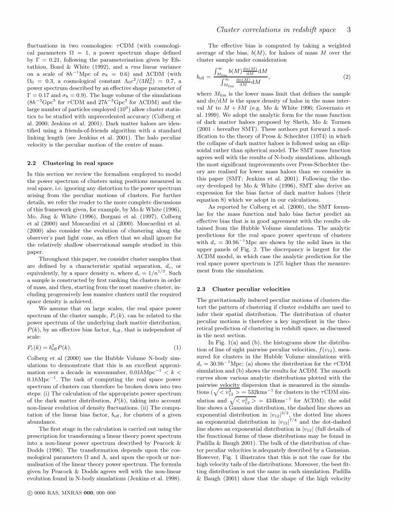
As reported by Colberg et al. (2000), the SMT formu-lae for the mass function and halo bias factor predict aneffective bias that is in good agreement with the results ob-tained from the Hubble Volume simulations. The analyticpredictions for the real space power spectrum of clusterswith dc = 30.9h−1Mpc are shown by the solid lines in theupper panels of Fig. 2. The discrepancy is largest for theΛCDM model, in which case the analytic prediction for thereal space power spectrum is 12% higher than the measure-ment from the simulation.

2.3 Cluster peculiar velocities

The gravitationally induced peculiar motions of clusters dis-tort the pattern of clustering if cluster redshifts are used toinfer their spatial distribution. The distribution of clusterpeculiar motions is therefore a key ingredient in the theo-retical prediction of clustering in redshift space, as discussedin the next section.

In Fig. 1(a) and (b), the histograms show the distribu-tion of line of sight pairwise peculiar velocities, f(v12), mea-sured for clusters in the Hubble Volume simulations withdc = 30.9h−1Mpc; (a) shows the distribution for the τCDMsimulation and (b) shows the results for ΛCDM. The smoothcurves show various analytic distributions plotted with thepairwise velocity dispersion that is measured in the simula-tions (

√

< v212 > = 532kms−1 for clusters in the τCDM sim-

ulation and√

< v212 > = 434kms−1 for ΛCDM); the solid

line shows a Gaussian distribution, the dashed line shows anexponential distribution in |v12|3/2, the dotted line showsan exponential distribution in |v12|7/4 and the dot-dashedline shows an exponential distribution in |v12| (full details ofthe functional forms of these distributions may be found inPadilla & Baugh 2001). The bulk of the distribution of clus-ter peculiar velocities is adequately described by a Gaussian.However, Fig. 1 illustrates that this is not the case for thehigh velocity tails of the distributions. Moreover, the best fit-ting distribution is not the same in each simulation. Padilla& Baugh (2001) show that the shape of the high velocity

c© 0000 RAS, MNRAS 000, 000–000


Figure 1. The histograms show the distribution of line of sight pairwise peculiar velocities of clusters with dc = 30.9h−1Mpc in theHubble Volume simulations: (a) shows the results for τCDM and (b) for ΛCDM, as indicated in the legend. The lower panels show thedistributions when a single cluster rms redshift error of δv = 500kms−1 is included. The smooth curves show theoretical distributionsplotted with the same variance in pairwise peculiar velocity that is measured from the simulations. In (a) and (b), solid lines showa Gaussian distribution, dashed lines show an exponential distribution in |v12|3/2, dotted lines are for an exponential distribution in|v12|7/4, and the dot-dashed lines show an exponential distribution in |v12|. In the lower panels, the variance includes the redshift errordescribed above, added in quadrature to the variance measured in the simulation. In (c) and (d) only the Gaussian distribution is plotted.

tail depends upon the degree of non-linear evolution of thedensity fluctuations. The distribution of peculiar velocitiesis therefore of interest in itself, being sensitive to the cos-mological parameters Ω and σ8, and to the power spectrumof density fluctuations (Croft & Efstathiou 1994b). Theseissues are explored in more detail using the Hubble Vol-ume simulations and other N-body simulations by Padilla& Baugh (2001).

The histograms in the lower panels of Fig. 1 show thedistribution of peculiar velocities after incorporating a singlecluster rms redshift measurement error of δv ≈ 500kms−1,appropriate for the Abell and APM cluster redshift sur-veys (Efstathiou et al. 1992). The resulting distributions aremuch broader and closer to Gaussian, as shown by the cor-

responding solid lines; in these cases the variance is given bythe sum in quadrature of the variance measured in the simu-lation and the rms redshift error stated above. The redshifterror dominates over the variance expected for gravitation-ally induced peculiar velocities for the models that we con-sider in this paper. We therefore make the approximationin subsequent calculations when comparing to APM datathat the variance in the pairwise peculiar velocity, includingerrors, is fixed at

√

< v212 > ∼ 850kms−1, regardless of the

model being studied. This in turn implies a single particlerms peculiar velocity of σ =

√

< v212 >/

√2 ≈ 600kms−1.

2.4 Clustering in redshift space - power spectrum

c© 0000 RAS, MNRAS 000, 000–000


2.4.1 Analytic model

The distortion of the power spectrum measured in redshiftspace generally displays two forms. On large scales, the am-plitude of the power spectrum is boosted due to coherentinflows into overdense regions and outflows from underdensevolumes (Kaiser 1987). On small scales, randomised motionswithin virialised structures cause a damping of power (e.g.Peacock 1999). Simple models have been developed that de-scribe the transition between this large and small scale be-haviour (Peacock & Dodds 1994, Cole, Fisher & Weinberg1995). These schemes have been shown to work reasonablywell for dark matter in N-body simulations (Cole, Fisher &Weinberg 1995; Hoyle et al. 1999). In this section we testwhether such models provide an accurate description of theredshift space power spectrum of clusters of galaxies; this isnecessary as we do not expect to find virialised structuresin the cluster distribution.

For scales that are still evolving according to linear per-turbation theory, the power spectrum in redshift space isgiven by

P sc (k, µ) = Pc(k)

(

1 + βµ2)2

, (3)

where Pc is the cluster power spectrum in real space, asdefined by equation 1, P s

c (k) is the cluster power spectrumin redshift space, β = f(Ω)/beff (f(Ω) is the logarithmicderivative of the fluctuation growth rate) and µ is the cosineof the angle between the wavevector k and the line of sight(Kaiser 1987; see also the discussion of this result in Cole,Fisher & Weinberg 1994).

Heuristic schemes have been put forward that extendthis model for the redshift space power spectrum down tosmall scales to include the effects of a random velocity dis-persion, under the assumption that the velocities are uncor-related with the density field:

P sc (k, µ) = Pc(k)

(

1 + βµ2)2

D(kµσv). (4)

For the case of a Gaussian distributed velocity dispersion,

D(kµσv) = exp(−k2µ2σ2v/2), (5)

whilst for an exponential distribution (Ballinger, Peacock &Heavens 1996),

D(kµσv) =1

1 + (kµσv)2 /2. (6)

The spherically averaged form of equation 4 for a Gaussianvelocity dispersion is given by Peacock & Dodds (1994):

P scl(k) = G(β, y)Pcl(k), (7)

where the function G(β, y) is given by

G(β, y) =√

π8

erf(y)

y5 [3β2 + 4βy2 + 4y4]

− exp(−y2)

4y4 [β2(3 + 2y2) + 4βy2], (8)

where β = f(Ω)/beff and y = kσv/(100kms−1Mpc−1). Er-rors in the determination of the cluster redshifts can be in-corporated into this model by adding the redshift error inquadrature to the rms peculiar velocity to redefine σv. Onthe scales that we consider, there is effectively no differencein the distortion to the power spectrum when a Gaussianor exponential distribution of velocity dispersion is adopted(see Fig. 3 of Ballinger, Heavens & Peacock 1996).

2.4.2 Comparison with simulation results

The analytic prediction for the spherically averaged clusterpower spectrum in redshift space is compared to the mea-surements from the Hubble Volume simulations in Fig. 2.In the simulations, the clustering pattern in redshift spaceis obtained by displacing clusters along the x-axis by anamount δx = vx/H0, where vx is the x-component of a clus-ter’s peculiar motion. The power spectrum of clusters in theHubble Volume simulation is computed using the techniquedescribed in detail by Jenkins et al. (1998), and is equiva-lent to employing a very high resolution grid to perform theFast Fourier Transform (FFT). Therefore, the scheme usedto assign clusters to the FFT grid does not influence therecovered power spectrum.

The lower panels in Fig. 2 show the ratio of the red-shift space to real space power spectrum as a function ofwavenumber. The dashed lines show the outcome of divid-ing the analytic prediction for the real space spectrum intothe prediction for the redshift space power spectrum, calcu-lated including the effects of cluster redshift errors. At smallwavenumbers (large scales) the ratios are in excellent agree-ment with the expectations from equation 3, which, usingthe approximation f(Ω) ≈ Ω0.6 predicts a ratio of 1.22 forclusters in τCDM and 1.15 in the ΛCDM simulation. Notethe latter value changes by less than 1% if the weak influenceof a non-zero cosmological constant on f(Ω) is taken intoaccount (Lahav et al. 1991). At high wavenumbers (smallscales) we find that there is no damping of the power spec-trum measured in redshift space when redshift errors areignored. The analytic model reproduces the boost in poweron large scales but predicts too much damping in the poweron small scales. If an error is included in the cluster redshifts,then the model predicts the same form of distortion foundin the simulations. The upper panels of Fig. 2 show thatin this case, the analytic model for the redshift space powerspectrum agrees with the simulation results to 15% or betterover the wavenumber range −2 < log(k/hMpc−1) < −1.

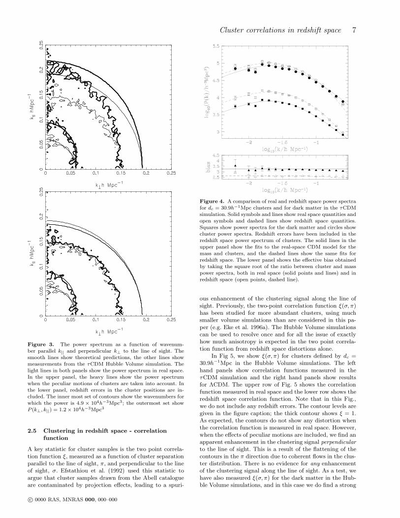
Further insight into the form of the distortion of the red-shift space power spectrum caused by cluster motions canbe obtained by plotting the power spectrum as a function ofwavenumber perpendicular (k⊥) and parallel (k||) to the line

of sight, P (k⊥, k||), where k =√

k2⊥ + k2

|| and µ = k||/k. We

plot P (k⊥, k||) for dc = 30.9h−1Mpc clusters in the τCDMHubble Volume simulation in Fig. 3. The smooth lines showanalytic predictions. The light solid lines show the real spacepower spectrum. In the upper panel, the heavy solid linesshow the redshift space power spectrum. In the lower panelthe heavy lines show the power spectrum in redshift spaceincluding the effects of redshift errors in the determination ofcluster positions. Two contour levels are plotted; the inner-most sets of contours show P (k⊥, k||) = 4.9 × 104h−3Mpc3

and the outermost set show P (k⊥, k||) = 1.2×104h−3Mpc3.On large scales, the analytic predictions are in excellentagreement with the measurements from the simulations, inreal space and in redshift space. In redshift space, the poweris enhanced on large scales in the k|| direction, displacingthe contour of fixed power to higher wavenumbers. On in-termediate scales, the distortion of the power spectrum isextremely sensitive to how well cluster redshifts are mea-sured. The magnitude of the error estimated in the redshifts

c© 0000 RAS, MNRAS 000, 000–000


Figure 2. The upper two panels show the real and redshift space power spectra for clusters with dc = 30.9h−1Mpc; the left panelsshow the results for τCDM and the right panels show results for ΛCDM. The lines show analytic predictions and the symbols showmeasurements made directly from the simulations. Real space quantities are shown by solid lines and squares. The redshift space powerspectrum measured in the simulations is shown by the circles. The dashed lines and triangles show the redshift space power spectrumafter incorporating a redshift error into the determination of cluster positions. The lower panels show the ratio between redshift spaceand real space power spectra as a function of wavenumber. Again, points show the ratio for the measurements in the simulation. Thecircles show the ratio when only peculiar motions are considered, the triangles show the ratio when redshift errors are also included.The dashed line shows the analytic prediction of the ratio, when cluster redshift errors are included and should be compared with thetriangles. The error bars are set by the number of modes per bin in wavenumber in the simulation.

of APM and Abell survey clusters dominates over the distor-tion due to the peculiar motions of the clusters. Therefore,on these scales, the boost in power given by equation 3 is apoor description of the power spectrum. Qualitatively, theanalytic model reproduces the form of the redshift space dis-tortion measured in the simulation. However, due to a smalldiscrepancy on intermediate scales between the predictedreal space power spectrum and the measurement from thesimulation (of around 10% in the amplitude of P (k)), thecontours do not coincide on this plot.

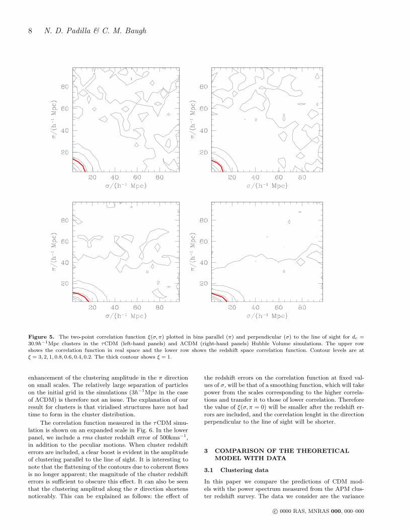
Finally, we compare the shapes of the redshift spacepower spectrum of clusters and dark matter in the τCDM

Hubble Volume simulation in Fig 4. The results for clustersinclude errors in the cluster redshift determination, as dis-cussed above. This plot illustrates that the redshift spacepower spectrum predicted by the model is in very goodagreement with that measured for the dark matter. The ef-fective bias measured in redshift space, as deduced by takingthe ratio of cluster and mass power spectra in redshift space,is somewhat lower than the bias measured in real space.However, the bias measured in redshift space is still inde-pendent of scale. A measurement of the cluster power spec-trum on large scales in redshift space would therefore yieldthe shape of the mass power spectrum in redshift space.

c© 0000 RAS, MNRAS 000, 000–000


Figure 3. The power spectrum as a function of wavenum-ber parallel k|| and perpendicular k⊥ to the line of sight. Thesmooth lines show theoretical predictions, the other lines showmeasurements from the τCDM Hubble Volume simulation. Thelight lines in both panels show the power spectrum in real space.In the upper panel, the heavy lines show the power spectrumwhen the peculiar motions of clusters are taken into account. Inthe lower panel, redshift errors in the cluster positions are in-cluded. The inner most set of contours show the wavenumbers forwhich the power is 4.9 × 104h−3Mpc3; the outermost set showP (k⊥, k||) = 1.2 × 104h−3Mpc3

2.5 Clustering in redshift space - correlation

function

A key statistic for cluster samples is the two point correla-tion function ξ, measured as a function of cluster separationparallel to the line of sight, π, and perpendicular to the lineof sight, σ. Efstathiou et al. (1992) used this statistic toargue that cluster samples drawn from the Abell catalogueare contaminated by projection effects, leading to a spuri-

Figure 4. A comparison of real and redshift space power spectrafor dc = 30.9h−1Mpc clusters and for dark matter in the τCDMsimulation. Solid symbols and lines show real space quantities andopen symbols and dashed lines show redshift space quantities.Squares show power spectra for the dark matter and circles showcluster power spectra. Redshift errors have been included in theredshift space power spectrum of clusters. The solid lines in theupper panel show the fits to the real-space CDM model for themass and clusters, and the dashed lines show the same fits forredshift space. The lower panel shows the effective bias obtainedby taking the square root of the ratio between cluster and masspower spectra, both in real space (solid points and lines) and inredshift space (open points, dashed line).

ous enhancement of the clustering signal along the line ofsight. Previously, the two-point correlation function ξ(σ, π)has been studied for more abundant clusters, using muchsmaller volume simulations than are considered in this pa-per (e.g. Eke et al. 1996a). The Hubble Volume simulationscan be used to resolve once and for all the issue of exactlyhow much anisotropy is expected in the two point correla-tion function from redshift space distortions alone.

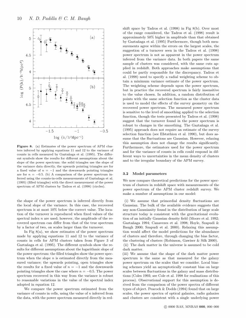
In Fig 5, we show ξ(σ, π) for clusters defined by dc =30.9h−1Mpc in the Hubble Volume simulations. The lefthand panels show correlation functions measured in theτCDM simulation and the right hand panels show resultsfor ΛCDM. The upper row of Fig. 5 shows the correlationfunction measured in real space and the lower row shows theredshift space correlation function. Note that in this Fig.,we do not include any redshift errors. The contour levels aregiven in the figure caption; the thick contour shows ξ = 1.As expected, the contours do not show any distortion whenthe correlation function is measured in real space. However,when the effects of peculiar motions are included, we find anapparent enhancement in the clustering signal perpendicular

to the line of sight. This is a result of the flattening of thecontours in the π direction due to coherent flows in the clus-ter distribution. There is no evidence for any enhancementof the clustering signal along the line of sight. As a test, wehave also measured ξ(σ, π) for the dark matter in the Hub-ble Volume simulations, and in this case we do find a strong

c© 0000 RAS, MNRAS 000, 000–000


Figure 5. The two-point correlation function ξ(σ, π) plotted in bins parallel (π) and perpendicular (σ) to the line of sight for dc =30.9h−1Mpc clusters in the τCDM (left-hand panels) and ΛCDM (right-hand panels) Hubble Volume simulations. The upper rowshows the correlation function in real space and the lower row shows the redshift space correlation function. Contour levels are atξ = 3, 2, 1, 0.8, 0.6, 0.4, 0.2. The thick contour shows ξ = 1.

enhancement of the clustering amplitude in the π directionon small scales. The relatively large separation of particleson the initial grid in the simulations (3h−1Mpc in the caseof ΛCDM) is therefore not an issue. The explanation of ourresult for clusters is that virialised structures have not hadtime to form in the cluster distribution.

The correlation function measured in the τCDM simu-lation is shown on an expanded scale in Fig. 6. In the lowerpanel, we include a rms cluster redshift error of 500kms−1,in addition to the peculiar motions. When cluster redshifterrors are included, a clear boost is evident in the amplitudeof clustering parallel to the line of sight. It is interesting tonote that the flattening of the contours due to coherent flowsis no longer apparent; the magnitude of the cluster redshifterrors is sufficient to obscure this effect. It can also be seenthat the clustering amplitud along the σ direction shortensnoticeably. This can be explained as follows: the effect of

the redshift errors on the correlation function at fixed val-ues of σ, will be that of a smoothing function, which will takepower from the scales corresponding to the higher correla-tions and transfer it to those of lower correlation. Thereforethe value of ξ(σ, π = 0) will be smaller after the redshift er-rors are included, and the correlation lenght in the directionperpendicular to the line of sight will be shorter.

3 COMPARISON OF THE THEORETICAL

MODEL WITH DATA

3.1 Clustering data

In this paper we compare the predictions of CDM mod-els with the power spectrum measured from the APM clus-ter redshift survey. The data we consider are the variance

c© 0000 RAS, MNRAS 000, 000–000


Figure 6. The two-point correlation function measured in red-shift space for clusters in the τCDM simulation. The same contourlevels used in Fig. 5 are plotted, with the thick contours showingξ = 1. In panel (a), gravitationally induced peculiar motions areconsidered. In (b), a rms cluster redshift error of 500kms−1 isalso included.

of counts in cells measured by Gaztanaga, Croft & Dalton(1995) and the power spectrum measured by Tadros, Ef-stathiou & Dalton (1998). Both measurements were madeusing sample B of the APM cluster redshift survey, as de-fined by Dalton et al. (1994).

Before confronting the model predictions with thesedata, we first compare the two measurements with one an-other. The variance of counts in cells is given by an integralover the power spectrum multiplied by the Fourier trans-form of the window used to smooth the density field (e.g.Peacock 1999)

σ2(R) =1

2π2

∫ ∞

0

dkk2P (k)W 2(kR). (9)

For a spherical top hat smoothing window of radius R,

W (kR) =3

(kR)3(sin(kR) − kR cos(kR)) . (10)

Figure 7. Testing the recovery of the power spectrum fromthe variance. The solid line shows a linear theory CDM powerspectrum with σ8 = 1 and Γ = 0.5. The points show the powerspectra recovered by applying equations 11 and 12 to the variance

computed from the linear theory power spectrum (as given byequation 9). The different symbols denote the results obtainedfor different assumptions about the slope of the power spectrum.

The integral is reasonably sharply peaked around a charac-teristic wavenumber for a particular smoothing scale. There-fore, we make the approximation that the variance measuredin a sphere of radius R can be related to the power spectrumat a specified wavenumber (see Peacock 1991 who gives theresult for a Gaussian smoothing window):

σ2(R) = ∆2(keff), (11)

where ∆2(k) = k3P (k)/2π2. If we consider power law spec-tra, P (k) ∝ kn, then the effective wavenumber is definedas:

keff =1

R[9I(n)]1/(n+3) , (12)

Here n is the logarithmic slope of the power spectrum atkeff , and the function I(n) is defined by (see also Gaztanaga1995):

I(n) =

∫ ∞

0

dxxn−4 (sin x − x cos x)2 . (13)

We demonstrate the accuracy of this transformation in Fig.7. The points show the power spectra recovered by applyingequations 11, 12 and 13 to the variance computed by inte-grating over the power spectrum shown by the solid line,which is our input spectrum (using equation 9). The differ-ent symbol types delineate the results obtained when dif-ferent assumptions are made about the shape of the powerspectrum. The most accurate answers are obtained when

c© 0000 RAS, MNRAS 000, 000–000


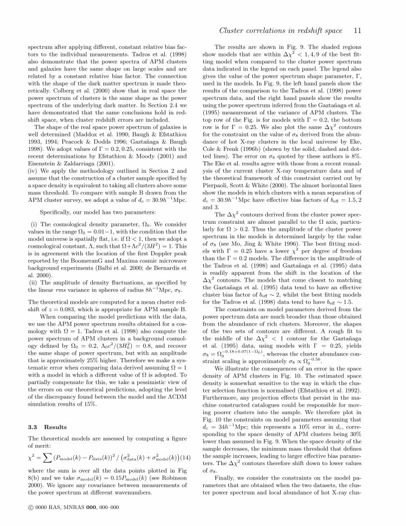
Figure 8. (a) Estimates of the power spectrum of APM clus-ters inferred by applying equations 11 and 12 to the variance ofcounts in cells measured by Gaztanaga et al. (1995). The differ-ent symbols show the results for different assumptions about the

slope of the power spectrum: the solid triangles use the slope ofthe variance data directly, the upwards pointing triangles are fora fixed value of n = −1 and the downwards pointing trianglesare for n = −0.5. (b) A comparison of the power spectrum in-ferred using the counts-in-cells measurements of Gaztanaga et al.(1995) (filled triangles) with the direct measurement of the powerspectrum of APM clusters by Tadros et al. (1998) (circles).

the shape of the power spectrum is inferred directly fromthe local slope of the variance. In this case, the recoveredspectrum is at most 10% below the correct value. The loca-tion of the turnover is reproduced when fixed values of thespectral index n are used; however, the amplitude of the re-covered spectrum can differ from that of the true spectrumby a factor of two, on scales larger than the turnover.

In Fig 8(a), we show estimates of the power spectrummade by applying equations 11 and 12 to the variance ofcounts in cells for APM clusters taken from Figure 3 ofGaztanaga et al. (1995). The different symbols show the re-sults for different assumptions about the logarithmic slope ofthe power spectrum: the filled triangles show the power spec-trum when the slope n is estimated directly from the mea-sured variance; the upwards pointing, open triangles showthe results for a fixed value of n = −1 and the downwardspointing triangles show the case where n = −0.5. The powerspectrum recovered in this way from the variance is robustto reasonable variations in the value of the spectral indexadopted in equation 12.

We compare the power spectrum estimated from thevariance of counts in cells, using the value of n inferred fromthe data, with the power spectrum measured directly in red-

shift space by Tadros et al. (1998) in Fig 8(b). Over mostof the range considered, the Tadros et al. (1998) result isapproximately 50% higher in amplitude than that obtainedby Gaztanaga et al. (1995) Furthermore, though both mea-surements agree within the errors on the largest scales, thesuggestion of a turnover seen in the Tadros et al. (1998)power spectrum is not as apparent in the power spectruminferred from the variance data. In both papers the samesample of clusters was considered, with the same cuts ap-plied in redshift. Both approaches make assumptions thatcould be partly responsible for the discrepancy. Tadros etal. (1998) need to specify a radial weighting scheme to ob-tain a minimum variance estimate of the power spectrum.The weighting scheme depends upon the power spectrum,but in practice the recovered spectrum is fairly insensitiveto the value chosen. In addition, a random distribution ofpoints with the same selection function as the cluster datais used to model the effects of the survey geometry on therecovered power spectrum. The measured power spectrumis sensitive to the level of smoothing applied to the selectionfunction, though the tests presented by Tadros et al. (1998)suggest that the turnover found in the power spectrum isrobust to changes in the smoothing. The Gaztanaga et al.(1995) approach does not require an estimate of the surveyselection function (see Efstathiou et al. 1990), but does as-sume that the fluctuations are Gaussian. However, relaxingthis assumption does not change the results significantly.Furthermore, the estimators used for the power spectrumand for the variance of counts in cells could respond in dif-ferent ways to uncertainties in the mean density of clustersand to the irregular boundary of the APM survey.

3.2 Model parameters

We now compare theoretical predictions for the power spec-trum of clusters in redshift space with measurements of thepower spectrum of the APM cluster redshift survey. Wemake a number of assumptions in our model:

(i) We assume that primordial density fluctuations areGaussian. The bulk of the available evidence suggests thatany non-Gaussianity found in the distribution of large scalestructure today is consistent with the gravitational evolu-tion of an initially Gaussian density field (Moore et al. 1992;Gaztanaga 1994; Canavezes et al. 1998; Hoyle, Szapudi &Baugh 2000; Szapudi et al. 2000). Relaxing this assump-tion would affect the model predictions for the abundanceof clusters and therefore, through changing the bias factor,the clustering of clusters (Robinson, Gawiser & Silk 2000).(ii) The dark matter in the universe is assumed to be colddark matter.(iii) We assume that the shape of the dark matter powerspectrum is the same as that measured for the galaxypower spectrum on the scales that we consider. Local bias-ing schemes yield an asymptotically constant bias on largescales between fluctuations in the galaxy and mass distribu-tions (Coles 1993; see Cole et al. 1998 for realisations of thisprocess). Observational support for this assumption is de-rived from the comparison of the power spectra of differenttypes of object. Peacock & Dodds (1994) found that on largescales, the power spectra of optical galaxies, radio galaxiesand clusters are consistent with a single underlying power

c© 0000 RAS, MNRAS 000, 000–000


spectrum after applying different, constant relative bias fac-tors to the individual measurements. Tadros et al. (1998)also demonstrate that the power spectra of APM clustersand galaxies have the same shape on large scales and arerelated by a constant relative bias factor. The connectionwith the shape of the dark matter spectrum is made theo-retically. Colberg et al. (2000) show that in real space thepower spectrum of clusters is the same shape as the powerspectrum of the underlying dark matter. In Section 2.4 wehave demonstrated that the same conclusions hold in red-shift space, when cluster redshift errors are included.

The shape of the real space power spectrum of galaxies iswell determined (Maddox et al. 1990; Baugh & Efstathiou1993, 1994; Peacock & Dodds 1996; Gaztanaga & Baugh1998). We adopt values of Γ = 0.2, 0.25, consistent with therecent determinations by Efstathiou & Moody (2001) andEisenstein & Zaldarriaga (2001).(iv) We apply the methodology outlined in Section 2 andassume that the construction of a cluster sample specified bya space density is equivalent to taking all clusters above somemass threshold. To compare with sample B drawn from theAPM cluster survey, we adopt a value of dc = 30.9h−1Mpc.

Specifically, our model has two parameters:

(i) The cosmological density parameter, Ω0. We considervalues in the range Ω0 = 0.01−1, with the condition that themodel universe is spatially flat, i.e. if Ω < 1, then we adopt acosmological constant, Λ, such that Ω+Λc2/(3H2) = 1. Thisis in agreement with the location of the first Doppler peakreported by the BoomeranG and Maxima cosmic microwavebackground experiments (Balbi et al. 2000; de Bernardis etal. 2000).(ii) The amplitude of density fluctuations, as specified bythe linear rms variance in spheres of radius 8h−1Mpc, σ8.

The theoretical models are computed for a mean cluster red-shift of z = 0.083, which is appropriate for APM sample B.

When comparing the model predictions with the data,we use the APM power spectrum results obtained for a cos-mology with Ω = 1. Tadros et al. (1998) also compute thepower spectrum of APM clusters in a background cosmol-ogy defined by Ω0 = 0.2, Λ0c

2/(3H20 ) = 0.8, and recover

the same shape of power spectrum, but with an amplitudethat is approximately 25% higher. Therefore we make a sys-tematic error when comparing data derived assuming Ω = 1with a model in which a different value of Ω is adopted. Topartially compensate for this, we take a pessimistic view ofthe errors on our theoretical predictions, adopting the levelof the discrepancy found between the model and the ΛCDMsimulation results of 15%.

3.3 Results

The theoretical models are assessed by computing a figureof merit:

χ2 =∑

(Pmodel(k) − Pdata(k))2 /(

σ2data(k) + σ2

model(k))

(14)

where the sum is over all the data points plotted in Fig8(b) and we take σmodel(k) = 0.15Pmodel(k) (see Robinson2000). We ignore any covariance between measurements ofthe power spectrum at different wavenumbers.

The results are shown in Fig. 9. The shaded regionsshow models that are within ∆χ2 < 1, 4, 9 of the best fit-ting model when compared to the cluster power spectrumdata indicated in the legend on each panel. The legend alsogives the value of the power spectrum shape parameter, Γ,used in the models. In Fig. 9, the left hand panels show theresults of the comparison to the Tadros et al. (1998) powerspectrum data, and the right hand panels show the resultsusing the power spectrum inferred from the Gaztanaga et al.(1995) measurement of the variance of APM clusters. Thetop row of the Fig. is for models with Γ = 0.2, the bottomrow is for Γ = 0.25. We also plot the same ∆χ2 contoursfor the constraint on the value of σ8 derived from the abun-dance of hot X-ray clusters in the local universe by Eke,Cole & Frenk (1996b) (shown by the solid, dashed and dot-ted lines). The error on σ8 quoted by these authors is 8%.The Eke et al. results agree with those from a recent reanal-ysis of the current cluster X-ray temperature data and ofthe theoretical framework of this constraint carried out byPierpaoli, Scott & White (2000). The almost horizontal linesshow the models in which clusters with a mean separation ofdc = 30.9h−1Mpc have effective bias factors of beff = 1.5, 2and 3.

The ∆χ2 contours derived from the cluster power spec-trum constraint are almost parallel to the Ω axis, particu-larly for Ω > 0.2. Thus the amplitude of the cluster powerspectrum in the models is determined largely by the valueof σ8 (see Mo, Jing & White 1996). The best fitting mod-els with Γ = 0.25 have a lower χ2 per degree of freedomthan the Γ = 0.2 models. The difference in the amplitude ofthe Tadros et al. (1998) and Gaztanaga et al. (1995) datais readily apparent from the shift in the location of the∆χ2 contours. The models that come closest to matchingthe Gaztanaga et al. (1995) data tend to have an effectivecluster bias factor of beff ∼ 2, whilst the best fitting modelsfor the Tadros et al. (1998) data tend to have beff ∼ 1.5.

The constraints on model parameters derived from thepower spectrum data are much broader than those obtainedfrom the abundance of rich clusters. Moreover, the shapesof the two sets of contours are different. A rough fit tothe middle of the ∆χ2 < 1 contour for the Gaztanagaet al. (1995) data, using models with Γ = 0.25, yields

σ8 = Ω−0.18+0.07(1−Ω0)0 , whereas the cluster abundance con-

straint scaling is approximately σ8 ∝ Ω−0.560 .

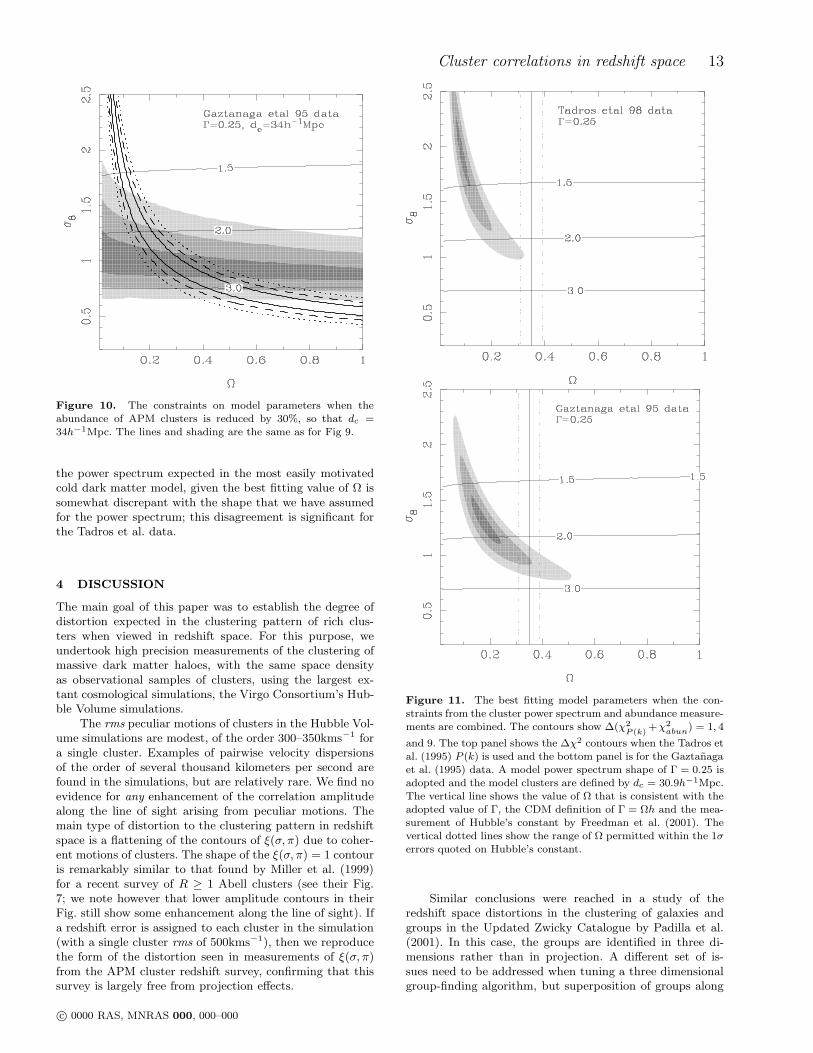
We illustrate the consequences of an error in the spacedensity of APM clusters in Fig. 10. The estimated spacedensity is somewhat sensitive to the way in which the clus-ter selection function is normalised (Efstathiou et al. 1992).Furthermore, any projection effects that persist in the ma-chine constructed catalogues could be responsible for mov-ing poorer clusters into the sample. We therefore plot inFig. 10 the constraints on model parameters assuming thatdc = 34h−1Mpc; this represents a 10% error in dc, corre-sponding to the space density of APM clusters being 30%lower than assumed in Fig. 9. When the space density of thesample decreases, the minimum mass threshold that definesthe sample increases, leading to larger effective bias parame-ters. The ∆χ2 contours therefore shift down to lower valuesof σ8.

Finally, we consider the constraints on the model pa-rameters that are obtained when the two datasets, the clus-ter power spectrum and local abundance of hot X-ray clus-

c© 0000 RAS, MNRAS 000, 000–000


Figure 9. The constraints on the model parameters σ8 and Ω0 from APM cluster power spectrum data. The shaded regions showcontours of ∆χ2 = 1, 4 and 9. The almost horizontal lines show parameter combinations for which the effective cluster bias is beff = 1.5, 2and 3. The left hand panels show the outcome of comparing the models to the Tadros et al. (1998) power spectrum data, the right handpanels are obtained using the power spectrum inferred from the Gaztanaga et al. (1995) variance of counts in cells. The upper row is formodels with Γ = 0.2, the lower row for Γ = 0.25. The lines show ∆χ2 contours for the constraint on σ8 and Ω0 from the local abundanceof hot X-ray clusters and are reproduced in each panel (Eke, Cole & Frenk 1996b).

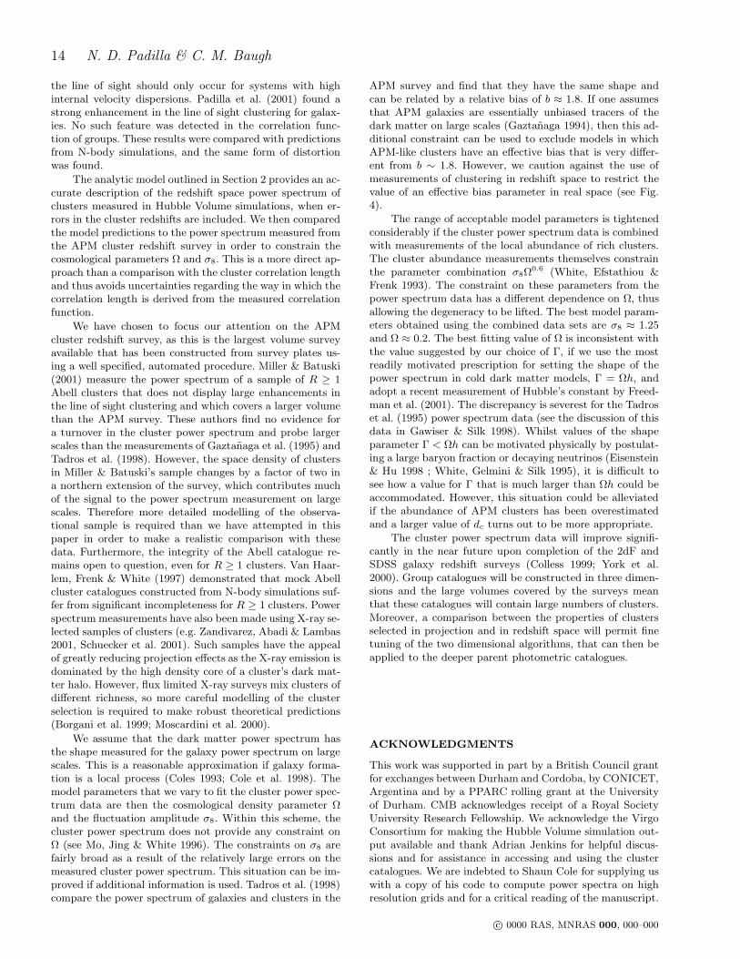
ters, are combined. In Fig. 11, we plot the ∆χ2 contoursafter adding the χ2 values from comparing the model to thepower spectrum data and to the observed cluster abundance.This operation assumes that the two datasets are indepen-dent. Due to the smaller errors, the cluster abundance con-straint has the largest influence on the resulting χ2 contours.The vertical line on each panel shows the value of Ω that isconsistent with the chosen Γ, given the recent determina-

tion of Hubble’s constant as H0 = 72 ± 8kms−1Mpc−1 byFreedman et al. (2001), and assuming that Γ = Ωh, whereH0 = 100hkms−1Mpc−1. The dotted lines indicate the rangeof values of Ω allowed following this prescription when the1σ errors on Hubble’s constant are taken into account. Thecombined dataset favours low values of Ω, with σ8 = 1–1.5for the Gaztanaga et al. measurement and σ8 = 1.6–2.3 forthe Tadros et al. power spectrum. In both cases, the shape of

c© 0000 RAS, MNRAS 000, 000–000


Figure 10. The constraints on model parameters when theabundance of APM clusters is reduced by 30%, so that dc =34h−1Mpc. The lines and shading are the same as for Fig 9.

the power spectrum expected in the most easily motivatedcold dark matter model, given the best fitting value of Ω issomewhat discrepant with the shape that we have assumedfor the power spectrum; this disagreement is significant forthe Tadros et al. data.

4 DISCUSSION

The main goal of this paper was to establish the degree ofdistortion expected in the clustering pattern of rich clus-ters when viewed in redshift space. For this purpose, weundertook high precision measurements of the clustering ofmassive dark matter haloes, with the same space densityas observational samples of clusters, using the largest ex-tant cosmological simulations, the Virgo Consortium’s Hub-ble Volume simulations.

The rms peculiar motions of clusters in the Hubble Vol-ume simulations are modest, of the order 300–350kms−1 fora single cluster. Examples of pairwise velocity dispersionsof the order of several thousand kilometers per second arefound in the simulations, but are relatively rare. We find noevidence for any enhancement of the correlation amplitudealong the line of sight arising from peculiar motions. Themain type of distortion to the clustering pattern in redshiftspace is a flattening of the contours of ξ(σ, π) due to coher-ent motions of clusters. The shape of the ξ(σ, π) = 1 contouris remarkably similar to that found by Miller et al. (1999)for a recent survey of R ≥ 1 Abell clusters (see their Fig.7; we note however that lower amplitude contours in theirFig. still show some enhancement along the line of sight). Ifa redshift error is assigned to each cluster in the simulation(with a single cluster rms of 500kms−1), then we reproducethe form of the distortion seen in measurements of ξ(σ, π)from the APM cluster redshift survey, confirming that thissurvey is largely free from projection effects.

Figure 11. The best fitting model parameters when the con-straints from the cluster power spectrum and abundance measure-ments are combined. The contours show ∆(χ2

P (k)+χ2

abun) = 1, 4

and 9. The top panel shows the ∆χ2 contours when the Tadros etal. (1995) P (k) is used and the bottom panel is for the Gaztanagaet al. (1995) data. A model power spectrum shape of Γ = 0.25 isadopted and the model clusters are defined by dc = 30.9h−1Mpc.The vertical line shows the value of Ω that is consistent with theadopted value of Γ, the CDM definition of Γ = Ωh and the mea-surement of Hubble’s constant by Freedman et al. (2001). Thevertical dotted lines show the range of Ω permitted within the 1σ

errors quoted on Hubble’s constant.

Similar conclusions were reached in a study of theredshift space distortions in the clustering of galaxies andgroups in the Updated Zwicky Catalogue by Padilla et al.(2001). In this case, the groups are identified in three di-mensions rather than in projection. A different set of is-sues need to be addressed when tuning a three dimensionalgroup-finding algorithm, but superposition of groups along

c© 0000 RAS, MNRAS 000, 000–000


the line of sight should only occur for systems with highinternal velocity dispersions. Padilla et al. (2001) found astrong enhancement in the line of sight clustering for galax-ies. No such feature was detected in the correlation func-tion of groups. These results were compared with predictionsfrom N-body simulations, and the same form of distortionwas found.

The analytic model outlined in Section 2 provides an ac-curate description of the redshift space power spectrum ofclusters measured in Hubble Volume simulations, when er-rors in the cluster redshifts are included. We then comparedthe model predictions to the power spectrum measured fromthe APM cluster redshift survey in order to constrain thecosmological parameters Ω and σ8. This is a more direct ap-proach than a comparison with the cluster correlation lengthand thus avoids uncertainties regarding the way in which thecorrelation length is derived from the measured correlationfunction.

We have chosen to focus our attention on the APMcluster redshift survey, as this is the largest volume surveyavailable that has been constructed from survey plates us-ing a well specified, automated procedure. Miller & Batuski(2001) measure the power spectrum of a sample of R ≥ 1Abell clusters that does not display large enhancements inthe line of sight clustering and which covers a larger volumethan the APM survey. These authors find no evidence fora turnover in the cluster power spectrum and probe largerscales than the measurements of Gaztanaga et al. (1995) andTadros et al. (1998). However, the space density of clustersin Miller & Batuski’s sample changes by a factor of two ina northern extension of the survey, which contributes muchof the signal to the power spectrum measurement on largescales. Therefore more detailed modelling of the observa-tional sample is required than we have attempted in thispaper in order to make a realistic comparison with thesedata. Furthermore, the integrity of the Abell catalogue re-mains open to question, even for R ≥ 1 clusters. Van Haar-lem, Frenk & White (1997) demonstrated that mock Abellcluster catalogues constructed from N-body simulations suf-fer from significant incompleteness for R ≥ 1 clusters. Powerspectrum measurements have also been made using X-ray se-lected samples of clusters (e.g. Zandivarez, Abadi & Lambas2001, Schuecker et al. 2001). Such samples have the appealof greatly reducing projection effects as the X-ray emission isdominated by the high density core of a cluster’s dark mat-ter halo. However, flux limited X-ray surveys mix clusters ofdifferent richness, so more careful modelling of the clusterselection is required to make robust theoretical predictions(Borgani et al. 1999; Moscardini et al. 2000).

We assume that the dark matter power spectrum hasthe shape measured for the galaxy power spectrum on largescales. This is a reasonable approximation if galaxy forma-tion is a local process (Coles 1993; Cole et al. 1998). Themodel parameters that we vary to fit the cluster power spec-trum data are then the cosmological density parameter Ωand the fluctuation amplitude σ8. Within this scheme, thecluster power spectrum does not provide any constraint onΩ (see Mo, Jing & White 1996). The constraints on σ8 arefairly broad as a result of the relatively large errors on themeasured cluster power spectrum. This situation can be im-proved if additional information is used. Tadros et al. (1998)compare the power spectrum of galaxies and clusters in the

APM survey and find that they have the same shape andcan be related by a relative bias of b ≈ 1.8. If one assumesthat APM galaxies are essentially unbiased tracers of thedark matter on large scales (Gaztanaga 1994), then this ad-ditional constraint can be used to exclude models in whichAPM-like clusters have an effective bias that is very differ-ent from b ∼ 1.8. However, we caution against the use ofmeasurements of clustering in redshift space to restrict thevalue of an effective bias parameter in real space (see Fig.4).

The range of acceptable model parameters is tightenedconsiderably if the cluster power spectrum data is combinedwith measurements of the local abundance of rich clusters.The cluster abundance measurements themselves constrainthe parameter combination σ8Ω

0.6 (White, Efstathiou &Frenk 1993). The constraint on these parameters from thepower spectrum data has a different dependence on Ω, thusallowing the degeneracy to be lifted. The best model param-eters obtained using the combined data sets are σ8 ≈ 1.25and Ω ≈ 0.2. The best fitting value of Ω is inconsistent withthe value suggested by our choice of Γ, if we use the mostreadily motivated prescription for setting the shape of thepower spectrum in cold dark matter models, Γ = Ωh, andadopt a recent measurement of Hubble’s constant by Freed-man et al. (2001). The discrepancy is severest for the Tadroset al. (1995) power spectrum data (see the discussion of thisdata in Gawiser & Silk 1998). Whilst values of the shapeparameter Γ < Ωh can be motivated physically by postulat-ing a large baryon fraction or decaying neutrinos (Eisenstein& Hu 1998 ; White, Gelmini & Silk 1995), it is difficult tosee how a value for Γ that is much larger than Ωh could beaccommodated. However, this situation could be alleviatedif the abundance of APM clusters has been overestimatedand a larger value of dc turns out to be more appropriate.

The cluster power spectrum data will improve signifi-cantly in the near future upon completion of the 2dF andSDSS galaxy redshift surveys (Colless 1999; York et al.2000). Group catalogues will be constructed in three dimen-sions and the large volumes covered by the surveys meanthat these catalogues will contain large numbers of clusters.Moreover, a comparison between the properties of clustersselected in projection and in redshift space will permit finetuning of the two dimensional algorithms, that can then beapplied to the deeper parent photometric catalogues.

ACKNOWLEDGMENTS

This work was supported in part by a British Council grantfor exchanges between Durham and Cordoba, by CONICET,Argentina and by a PPARC rolling grant at the Universityof Durham. CMB acknowledges receipt of a Royal SocietyUniversity Research Fellowship. We acknowledge the VirgoConsortium for making the Hubble Volume simulation out-put available and thank Adrian Jenkins for helpful discus-sions and for assistance in accessing and using the clustercatalogues. We are indebted to Shaun Cole for supplying uswith a copy of his code to compute power spectra on highresolution grids and for a critical reading of the manuscript.

c© 0000 RAS, MNRAS 000, 000–000


REFERENCES

Abadi, M.G., Lambas, D.G., Muriel, H., 1998, ApJ, 507, 526.

Bahcall, N.A., Cen, R.Y., 1992, ApJ, 398, L81.

Bahcall, N.A., Cen, R.Y., Gramann, M., 1994, ApJ, 430, L13.

Bahcall, N.A., Soneira, R.M., 1983, ApJ, 270, 20.

Bahcall, N.A., Soneira, R.M., Burgett, W.S., 1986, ApJ, 311, 15.

Bahcall, N.A., West, M.J., 1992, ApJ, 392, 419.

Balbi, A., et al. , 2000, ApJ, 545, L1.

Ballinger, W.E., Peacock, J.A., Heavens, A.F., 1996, MNRAS,282, 877.

Baugh, C.M., Efstathiou, G., 1993, MNRAS, 265, 145.

Baugh, C.M., Efstathiou, G., 1994, MNRAS, 267, 323.

Baugh, C.M., Gaztanaga, E. & Efstathiou, G., 1995, MNRAS,274, 1049

Blanchard, A., Bartlett, J.G., 1998, Astron. & Astroph., 332, L49.

Borgani, S., Moscardini, L., Plionis, M., Gorski, K.M., Holtzman,J., Klypin, A., Primack, J.R., Smith, C.C., Stompor, R., 1997,New Astronomy, 1, 321.

Borgani, S., Plionis, M., Kolokotronis, V., 1999, MNRAS, 305,866.

Canavezes, A., et al. , 1998, MNRAS, 297, 777.

Colberg, J.M., et al. , 2000, MNRAS, 319, 209.

Cole, S., Fisher, K.B., Weinberg, D.H., 1994, MNRAS, 267, 785.

Cole, S., Fisher, K.B., Weinberg, D.H., 1995, MNRAS, 275, 515.

Cole, S., Hatton, S.J., Weinberg, D.H., Frenk, C.S., 1998, MN-RAS, 300, 945.

Coles, P., 1993, MNRAS, 262, 1065.

Colless, M., 1999, Phil. Trans. Roy. Soc. A., 357., 105.

Collins, C.A., Guzzo, L., Boehringer, H., Schuecker, P, Chincar-ini, G., Cruddace, R., De Grandi, S, MacGillivray, H.T., Neu-mann, D.M., Schindler, S., Shaver, P., Voges, W., 2000, astro-ph/0008245.

Croft, R.A.C., Efstathiou, G., 1994a, MNRAS, 267, 390.

Croft, R.A.C., Efstathiou, G., 1994b, MNRAS, 268, L23.

Croft, R.A.C., Dalton, G.B., Efstathiou, G., Sutherland, W.J.,Maddox, S.J., 1997, MNRAS, 291, 305.

Dalton, G.B., Efstathiou, G., Maddox, S.J., Sutherland, W.J.,1992, ApJ, 390, L1.

Dalton, G.B., Efstathiou, G., Maddox, S.J., Sutherland, W.J.,1994, MNRAS, 269, 151.

Dalton, G.B., Maddox, S.J., Sutherland, W.J., Efstathiou, G.,1997, MNRAS, 289, 263.

de Bernardis, P., et al. , 2000, Nature, 404, 955.

Efstathiou, G., Bond, J.R., White, S.D.M., 1992, MNRAS, 258,1P.

Efstathiou, G., Dalton, G.B., Sutherland, W.J., Maddox, S.J.,1992, MNRAS, 257, 125.

Efstathiou, G., Kaiser, N., Saunders, W., Lawrence, A., Rowan-Robinson, M., Ellis, R.S., Frenk, C.S., 1990, MNRAS, 247,10P.

Efstathiou, G., Moody, S.J., 2001, MNRAS submitted, astro-ph/0010478.

Eisenstein, D., Hu, W., 1998, ApJ, 496, 605.

Eisenstein, D., Zaldarriaga, M., 2001, ApJ, 546, 2.

Eke, V.R., Cole, S., Frenk, C.S., 1996b, MNRAS, 282, 263.

Eke, V.R., Cole, S., Frenk, C.S., Navarro, J.F., 1996a, MNRAS,281, 703.

Eke, V.R., Cole, S., Frenk, C.S., Henry, J.P., 1998, MNRAS, 298,1145.

Freedman, W.L., et al. , 2001, ApJ, in press, astro-ph/0012376

Gawiser, E., Silk, J., 1998, Science, 280, 1405.

Gaztanaga, E., 1994, MNRAS, 268, 913.

Gaztanaga, E., Baugh, C.M., 1998, MNRAS, 294, 229.

Gaztanaga, E., Croft, R.A.C., Dalton, G.B., 1995, MNRAS, 276,336.

Governato, F., Babul, A., Quinn, T., Tozzi, P., Baugh, C.M.,Katz, N., Lake, G., 1999, MNRAS, 307, 949.

Hoyle, F., Baugh, C. M., Shanks, T., Ratcliffe, A., 1999, MNRAS,

309, 659.Hoyle, F., Szapudi, I., Baugh, C. M., 2000, MNRAS, 317, L51.Jenkins, A., Frenk, C.S., Pearce, F.R., Thomas, P.A., Colberg,

J.M., White, S.D.M., Couchman, H.M.P., Peacock, J.A., Ef-stathiou, G., Nelson, A.H., 1998, ApJ, 499, 20.

Jenkins, A., Frenk, C.S., White, S.D.M., Colberg, J.M., Cole, S.,Evrard, A.E., Couchman, H.M.P., Yoshida, N., 2001, MN-RAS, 321, 372.

Klypin, A.A., Kopylov, A.I., 1983, Soviet Astron. Lett., 9, 41.Lahav, O., Lilje, P.B., Primack, J.R., Rees, M.J., 1991, MNRAS,

251, 128.Lucey, J. R., 1983, MNRAS, 204, 33.Lumsden, S.L., Nichol, R.C., Collins, C.A., Guzzo, L., 1992, MN-

RAS, 258, 1.Kaiser, N., 1987, MNRAS, 227, 1.Maddox, S.J., Efstathiou, G., Sutherland, W.J., Loveday, J., 1990,

MNRAS, 242, 43P.Miller, C.J., Batuski, D.J., Slingend, K.A., Hill, J.M., 1999, ApJ,

523, 492.Miller, C.J., Batuski, D.J., 2001, ApJ, in press, astro-ph/0002295.Mo, H.J., White, S.D.M., 1996, MNRAS, 282, 347.Mo, H.J., Jing, Y.P., White, S.D.M., 1996, MNRAS, 282, 1096.Moore, B., Frenk, C.S., Weinberg, D.H., Saunders, W., Lawrence,

A., Ellis, R.S., Kaiser, N., Efstathiou, G., Rowan-Robinson,M., 1992, MNRAS, 256, 477.

Moscardini, L., Matarrese, S., Lucchin, E., Rosati, P., 2000, MN-RAS, 316, 283.

Padilla, N.D., Baugh, C.M., 2001, in preparation.Padilla, N.D., Merchan, M.E., Valotto, C.A., Lambas, D.G.,

Maia, M.A.G., 2001, ApJ, in press, astro-ph/0102372.Peacock, J. A., 1991, MNRAS, 253, P1.Peacock, J. A., 1999, Cosmological Physics, Cambridge.Peacock, J. A. & Dodds, S. J., 1994, MNRAS, 267, 1020.Peacock, J. A. & Dodds, S. J., 1996, MNRAS, 280, L19.Peacock, J. A. & West, M.J., 1992, MNRAS, 259, 494.Pierpaoli, E., Scott, D., White, M., 2000, Mod. Phys. Lett. A.,

15, 1357.Postman, M., Huchra, J.P., Geller, M.J., 1992, ApJ, 384, 404.Press, W.H., Schechter, P., 1974, ApJ., 187, 425.Robinson, J., 2000, astro-ph/0004023.Robinson, J., Gawiser, E., Silk, J., 2000, ApJ, 532, 1.Schuecker, P., et al. , 2001, Astron & Astroph., 368, 86.Sheth, R.K., Mo, H.J., Tormen, G., 2001, MNRAS, 323, 1Sutherland, W., 1988, MNRAS, 234, 159.Sutherland, W.J., Efstathiou, G., 1991, MNRAS, 248, 159.Szapudi, I., Branchini, E., Frenk, C.S., Maddox, S., Saunders, W.,

2000, MNRAS, 318, L45.Tadros, H., Efstathiou, G., Dalton, G., 1998, MNRAS, 296, 995.van Haarlem, M.P., Frenk, C.S., White, S.D.M., 1997, 287, 817.Watanabe, T., Matsubara, T., Suto, Y., 1994, ApJ, 432, 17.White, M., Gelmini, G., Silk, J., 1995, Phys. Rev. D., 51, 2669.White, S.D.M., Efstathiou, G., Frenk, C.S., 1993, MNRAS, 262,

1023.White, S.D.M., Frenk, C.S., Davis, M., Efstathiou, G., 1987, ApJ,

313, 505.York, D.G., et al. , 2000, AJ, 120, 1579.Zandivarez, A., Abadi, M.G., Lambas, D.G., 2001, MNRAS, in

press, astro-ph/0103378.

c© 0000 RAS, MNRAS 000, 000–000

http://arxiv.org/abs/astro-ph/0008245









Documents

Cluster correlations in redshift space