Embed Size (px)
Citation preview
University of Calgary
PRISM: University of Calgary's Digital Repository
Graduate Studies The Vault: Electronic Theses and Dissertations
2019-06-12
Cluster analysis of correlated non-Gaussian
continuous data via finite mixtures of Gaussian
copula distributions
Burak, Katherine L.
Burak, K. L. (2019). Cluster analysis of correlated non-Gaussian continuous data via finite
mixtures of Gaussian copula distributions (Unpublished master's thesis). University of Calgary,
Calgary, AB.
http://hdl.handle.net/1880/110497
master thesis
University of Calgary graduate students retain copyright ownership and moral rights for their
thesis. You may use this material in any way that is permitted by the Copyright Act or through
licensing that has been assigned to the document. For uses that are not allowable under
copyright legislation or licensing, you are required to seek permission.
Downloaded from PRISM: https://prism.ucalgary.ca

UNIVERSITY OF CALGARY
Cluster analysis of correlated non-Gaussian continuous data via finite mixtures of Gaussian
copula distributions
by
Katherine L. Burak
A THESIS
SUBMITTED TO THE FACULTY OF GRADUATE STUDIES
IN PARTIAL FULFILLMENT OF THE REQUIREMENTS FOR THE
DEGREE OF MASTER OF SCIENCE
GRADUATE PROGRAM IN MATHEMATICS AND STATISTICS
CALGARY, ALBERTA
JUNE, 2019
c© Katherine L. Burak 2019
Abstract
Model-based cluster analysis in non-Gaussian settings is not straightforward due to a lack of
standard models for non-Gaussian data. In this thesis, we adopt the class of Gaussian cop-
ula distributions (GCDs) to develop a flexible model-based clustering methodology that can
accommodate a variety of correlated, non-Gaussian continuous data, where variables may
have different marginal distributions and come from different parametric families. Unlike
conventional model-based approaches that rely on the assumption of conditional indepen-
dence, GCDs model conditional dependence among the disparate variables using the matrix
of so-called normal correlations. We outline a hybrid approach to cluster analysis that com-
bines the method of inference functions for margins (IFM) and the parameter-expanded
EM (PX-EM) algorithm. We then report simulation results to investigate the performance
of our methodology. Finally, we highlight the applications of this research by applying this
methodology to a dataset regarding the purchases made by clients of a wholesale distributor.
ii

Acknowledgements
I would like to express my gratitude to my supervisor, Dr. A.R. de Leon, for his guidance
throughout this entire process. I am very grateful for the extensive knowledge and leadership
he has provided me during my master’s degree.
I would also like to thank my co-supervisor, Dr. J. Wu, and Drs. X. Lu and K. Kopciuk
for acting as my committee members and providing valuable feedback on my thesis.
Finally, I would like to thank my parents for their endless support; without them, this
truly would not have been possible.
iii
Table of Contents
Abstract ii
Acknowledgements iii
Table of Contents iv
List of Figures and Illustrations vi
List of Tables vii
1 Introduction 11.1 Joint models for non-Gaussian continuous data . . . . . . . . . . . . . . . . . 1
1.1.1 Gaussian copula distributions . . . . . . . . . . . . . . . . . . . . . . 31.2 Cluster analysis . . . . . . . . . . . . . . . . . . . . . . . . . . . . . . . . . . 51.3 EM algorithm . . . . . . . . . . . . . . . . . . . . . . . . . . . . . . . . . . . 7
1.3.1 PX-EM algorithm . . . . . . . . . . . . . . . . . . . . . . . . . . . . . 91.4 Inference functions for margins . . . . . . . . . . . . . . . . . . . . . . . . . 101.5 Overview of thesis . . . . . . . . . . . . . . . . . . . . . . . . . . . . . . . . . 11
2 Model-based clustering with Gaussian copula distributions 122.1 Finite mixtures of GCDs . . . . . . . . . . . . . . . . . . . . . . . . . . . . . 122.2 PXEM-IFM algorithm . . . . . . . . . . . . . . . . . . . . . . . . . . . . . . 142.3 Discussion . . . . . . . . . . . . . . . . . . . . . . . . . . . . . . . . . . . . . 18
3 Simulations 193.1 Simulation design . . . . . . . . . . . . . . . . . . . . . . . . . . . . . . . . . 19
3.1.1 Parameter settings . . . . . . . . . . . . . . . . . . . . . . . . . . . . 203.2 Model selection criterion . . . . . . . . . . . . . . . . . . . . . . . . . . . . . 23
3.2.1 Bayesian information criterion . . . . . . . . . . . . . . . . . . . . . . 233.2.2 Clustering indices . . . . . . . . . . . . . . . . . . . . . . . . . . . . . 243.2.3 Relative bias . . . . . . . . . . . . . . . . . . . . . . . . . . . . . . . 26
3.3 Results . . . . . . . . . . . . . . . . . . . . . . . . . . . . . . . . . . . . . . . 263.3.1 Simulation 1 . . . . . . . . . . . . . . . . . . . . . . . . . . . . . . . . 263.3.2 Simulation 2 . . . . . . . . . . . . . . . . . . . . . . . . . . . . . . . . 283.3.3 Simulation 3 . . . . . . . . . . . . . . . . . . . . . . . . . . . . . . . . 303.3.4 Discussion . . . . . . . . . . . . . . . . . . . . . . . . . . . . . . . . . 33
iv

4 Application 354.1 Overview of dataset . . . . . . . . . . . . . . . . . . . . . . . . . . . . . . . . 354.2 Results . . . . . . . . . . . . . . . . . . . . . . . . . . . . . . . . . . . . . . . 374.3 Discussion . . . . . . . . . . . . . . . . . . . . . . . . . . . . . . . . . . . . . 38
5 Conclusion 425.1 Summary . . . . . . . . . . . . . . . . . . . . . . . . . . . . . . . . . . . . . 425.2 Future work . . . . . . . . . . . . . . . . . . . . . . . . . . . . . . . . . . . . 43
Bibliography 44
v

List of Figures and Illustrations
3.1 Plot of true clusters (K = 3, high separation) . . . . . . . . . . . . . . . . . 203.2 Plot of true clusters (K = 2, moderate separation) . . . . . . . . . . . . . . . 213.3 Plot of true clusters (K = 3, mild separation) . . . . . . . . . . . . . . . . . 223.4 Plot of clusters obtained via GCD (K = 3, high separation) . . . . . . . . . 273.5 Plot of clusters obtained via GCD (K = 2, moderate separation) . . . . . . . 293.6 Plot of clusters obtained via GCD (K = 3, mild separation) . . . . . . . . . 32
4.1 Histograms of continuous variables (wholesale dataset) . . . . . . . . . . . . 394.2 Plot of clusters obtained via GCD (wholesale dataset) . . . . . . . . . . . . . 404.3 Plot of data coloured by channel variable (wholesale dataset) . . . . . . . . . 41
vi

List of Tables
3.1 Parameter settings (K = 3, high separation) . . . . . . . . . . . . . . . . . . 203.2 Parameter settings (K = 2, moderate separation) . . . . . . . . . . . . . . . 213.3 Parameter settings (K = 3, mild separation) . . . . . . . . . . . . . . . . . . 223.4 Average parameter estimates and relative bias after R = 100 repeats (K = 3,
high separation) . . . . . . . . . . . . . . . . . . . . . . . . . . . . . . . . . . 263.5 Number of components, BIC, Rand index, Jaccard index and Fowlkes-Mallows
index (K = 3, high separation) . . . . . . . . . . . . . . . . . . . . . . . . . 273.6 Number of components, BIC, Rand index, Jaccard index and Fowlkes-Mallows
index assuming conditional independence (K = 3, high separation) . . . . . . 283.7 Average parameter estimates and relative bias after R = 100 repeats (K = 2,
moderate separation) . . . . . . . . . . . . . . . . . . . . . . . . . . . . . . . 283.8 Number of components, BIC, Rand index, Jaccard index and Fowlkes-Mallows
index (K = 2, moderate separation) . . . . . . . . . . . . . . . . . . . . . . . 293.9 Number of components, BIC, Rand index, Jaccard index and Fowlkes-Mallows
index assuming conditional independence (K = 2, moderate separation) . . . 303.10 Average parameter estimates and relative bias after R = 50 repeats (K = 3,
mild separation) . . . . . . . . . . . . . . . . . . . . . . . . . . . . . . . . . . 313.11 Number of components, BIC, Rand index, Jaccard index and Fowlkes-Mallows
index (K = 3, mild separation) . . . . . . . . . . . . . . . . . . . . . . . . . 313.12 Number of components, BIC, Rand index, Jaccard index and Fowlkes-Mallows
index assuming conditional independence (K = 3, mild separation) . . . . . 32
4.1 Number of components and BIC (wholesale dataset) . . . . . . . . . . . . . . 374.2 Component parameter estimates (wholesale dataset) . . . . . . . . . . . . . . 374.3 Number of components and BIC assuming componentwise conditional inde-
pendence between variables (wholesale dataset) . . . . . . . . . . . . . . . . 37
vii

Chapter 1
Introduction
Non-Gaussian continuous data pertains to data comprised of a mixture of continuous dis-
parate variables with a variety of marginal distributions. Such data is ubiquitous in many
disciplines such as medicine and health care, genetics, marketing and finance. Although
non-Gaussian data commonly arises, there are a lack of standard models for data of this
nature and some current techniques assume conditional independence between the variables,
which can be problematic with regards to the data analysis. In this chapter, we review the
literature on current techniques for the analysis of non-Gaussian continuous data, as well as
introduce copula models as a flexible model for such data. We introduce the Expectation-
Maximization (EM) algorithm with applications in cluster analysis. Additionally, we outline
the methodology behind the parameter-expanded EM algorithm, a variant of the EM al-
gorithm, and inference functions for margins. Furthermore, we provide an overview of this
thesis and its objectives.
1.1 Joint models for non-Gaussian continuous data
In order to analyze multivariate data, we must first specify a joint distribution of the data.
However, in practice, this can be difficult to construct, especially if the variables have different
marginal distributions. Some current techniques, such as generalized linear mixed models
1
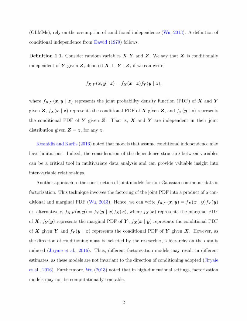
(GLMMs), rely on the assumption of conditional independence (Wu, 2013). A definition of
conditional independence from Dawid (1979) follows.
Definition 1.1. Consider random variables X,Y and Z. We say that X is conditionally
independent of Y given Z, denoted X ⊥⊥ Y | Z, if we can write
fX,Y (x,y | z) = fX(x | z)fY (y | z),
where fX,Y (x,y | z) represents the joint probability density function (PDF) of X and Y
given Z, fX(x | z) represents the conditional PDF of X given Z, and fY (y | z) represents
the conditional PDF of Y given Z. That is, X and Y are independent in their joint
distribution given Z = z, for any z.
Kosmidis and Karlis (2016) noted that models that assume conditional independence may
have limitations. Indeed, the consideration of the dependence structure between variables
can be a critical tool in multivariate data analysis and can provide valuable insight into
inter-variable relationships.
Another approach to the construction of joint models for non-Gaussian continuous data is
factorization. This technique involves the factoring of the joint PDF into a product of a con-
ditional and marginal PDF (Wu, 2013). Hence, we can write fX,Y (x,y) = fX(x | y)fY (y)
or, alternatively, fX,Y (x,y) = fY (y | x)fX(x), where fX(x) represents the marginal PDF
of X, fY (y) represents the marginal PDF of Y , fX(x | y) represents the conditional PDF
of X given Y and fY (y | x) represents the conditional PDF of Y given X. However, as
the direction of conditioning must be selected by the researcher, a hierarchy on the data is
induced (Jiryaie et al., 2016). Thus, different factorization models may result in different
estimates, as these models are not invariant to the direction of conditioning adopted (Jiryaie
et al., 2016). Furthermore, Wu (2013) noted that in high-dimensional settings, factorization
models may not be computationally tractable.
2
1.1.1 Gaussian copula distributions
Copula models are a flexible alternative to jointly model non-Gaussian continuous data.
As illustrated by Ren (2016), the objective is to specify the joint distribution of the data
by transforming the disparate variables into uniform variables via the probability integral
transform (PIT), and then using a copula to ‘glue’ together the margins (Jiryaie et al., 2016).
This section follows the work presented in Jiryaie et al. (2016) and Ren (2016).
LetX = (X1, ..., XP )> be a vector of continuous variables with corresponding cumulative
distribution functions (CDFs) FX1(X1), . . . , FXP(XP ). Recall that, via the PIT, FXj
(Xj) =
Uj ∼ uniform[0, 1], ∀j ∈ 1, . . . , P . Hence, as defined by Ren (2016), we can specify the P -
dimensional joint distribution function FX(x) = FX1,...,XP(x1, . . . , xP ) via the P -dimensional
copula C(u1, . . . , uP ) as
FX(x) = FU (u) = C(u1, . . . , uP ), (1.1)
where uj = FXj(xj) is a realization of Uj, j = 1, . . . , P . Thus, we can construct the joint
distribution of X1, ..., XP from their respective marginal distributions and the joint CDF
of U1, ..., UP , FU (u) = FU1,...,UP(u1, . . . , uP ), which we call a copula. Therefore, a copula is
simply the joint CDF of, possibly dependent, identically distributed uniform[0, 1] random
variables (Ren, 2016). Jiryaie et al. (2016) states that copulas allow great flexibility in mixed
data analysis as the margins do not need to come from the same parametric family. A formal
definition by Nelsen (2006) is provided below.
Definition 1.2. Let I = [0, 1] and IP = [0, 1]P , the P -dimensional unit hyperrectangle. A
P-dimensional copula is a function C(·) from IP to I with the following properties:
1. For every u in IP , C(u) = 0 if at least one coordinate of u is 0, and if all coordinates of
u are 1 except uj, then C(u) = uj.
3

2. For every hyperrectangle [a, b] = [a1, b1] × · · · × [aP , bP ], such that 0 ≤ aj ≤ bj ≤ 1, for
all j = 1, . . . , P ,
VC([a, b]) ≥ 0,
where VC([a, b]) is the volume of [a, b]. That is, C(u) is P -increasing.
Thus, we can construct a joint model for disparate continuous variables with a variety
of marginal distributions that need not be from the same parametric family. The copula is
a powerful and flexible tool in constructing joint multivariate distributions that do not rely
on limiting distributional assumptions.
Choosing an appropriate copula to join together the variable’s marginal distributions is
contingent upon the sufficiency of the copula’s dependence parameter to represent the data’s
dependency structure (Jiryaie et al., 2016). The Gaussian copula is a popular choice due to
its attractive mathematical properties. Given continuous variables X1 ∼ FX1(x1), . . . , XP ∼
FXP(xP ) with joint distribution function FX1,...,XP
(x1, . . . , xP ), the P -dimensional Gaussian
copula distribution (GCD) is defined as
FX(x; Θ,R) = ΦP (Φ−1(u1), . . . ,Φ−1(uP ); R), (1.2)
where Φ−1(u) is the standard normal quantile function, ΦP (u1, . . . , uP ; R) is the P -
dimensional Gaussian CDF with mean vector 0 and correlation matrix R, u1, . . . , uP are re-
alizations of their respective PITs U1 = FX1(X1;θ1) ∼ uniform[0, 1], . . . , UP = FXP(XP ;θP )
∼ uniform[0, 1], Θ = (θ>1 , . . . ,θ>P )>, and R is the correlation matrix of normal scores
Q1 = Φ−1(U1) ∼ N(0, 1), . . . , QP = Φ−1(UP ) ∼ N(0, 1). Here, θj can be a vector or a
scalar depending on the parameter of FXj(xj); for example, if X1 ∼ Gamma(α, β) and
X2 ∼ Exponential(λ), Θ = (θ>1 , θ2)>, where θ1 = (α, β)> and θ2 is simply the scalar λ. The
PDF fX(x; Θ,R) corresponding to the GCD defined in (1.2) is given by
4
fX(xi; Θ,R) =φP (qi1, . . . , qiP ; 0,R)∏P
j=1 φ(qij)
P∏j=1
fXj(xij;θj), (1.3)
where φ(qij) is the standard Gaussian PDF, φP (qi1, . . . , qiP ; 0,R) is the P -dimensional Gaus-
sian PDF with mean vector 0 and correlation matrix R, qij = Φ−1(uij) = Φ−1(FXj(xij;θj)),
and fXj(xij;θj) is the marginal PDF of Xij.
GCDs are a useful and flexible tool in the analysis of non-Gaussian data as they describe
dependence between variables in a similar fashion as Gaussian distributions (Jiryaie et al.,
2016).
1.2 Cluster analysis
Cluster analysis is the process of identifying meaningful groups in data. The main objective of
cluster analysis is to determine the underlying structure of the data without having any prior
information on what this structure might be. Typically, cluster analysis is either performed
via a distance-based or model-based approach. However, over the last ten years, the use of
mixture models for cluster analysis has dramatically increased (Andrews and McNicholas,
2012). A random vector X is from a parametric finite mixture distribution if, for all X = x,
we can write the PDF of X as
f(x; Θ,π) =K∑k=1
πkfk(x;θk), (1.4)
where π = (π1, . . . , πK)>, πk > 0 is the kth mixing proportion such that∑K
k=1 πk = 1,
fk(x;θk) is the PDF of the kth component, and Θ = (θ>1 , . . . ,θ>K)>, where θk = (θ>k1, . . . ,
θ>kP )> is the vector of parameters for component k = 1, . . . , K (Franczak, 2014). Typi-
cally, component densities are chosen to be of the same type (McNicholas, 2016); that is,
fk(x;θk) = f(x;θk) for all k = 1, ..., K. Historically, the multivariate Gaussian has been a
popular choice for the component densities due to its mathematical tractability and flexibil-
5
ity (Franczak, 2014). However, such approaches may not be suitable when we are concerned
with the analysis of non-Gaussian data, which can be comprised of a mixture of possibly
a large number of disparate variables with a variety of marginal distributions. Unlike con-
ventional model-based approaches that rely on the assumption of conditional independence,
GCDs model conditional dependence for each component among the disparate variables us-
ing the matrix of so-called normal correlations. Thus, we introduce a mixture of GCDs
as a flexible clustering methodology for the non-Gaussian continuous data. The PDF of a
mixture of GCDs is given by
f(xi; Θ,R1, . . . ,RK ,π) =K∑k=1
πkfk(xi;θk,Rk), (1.5)
where
fk(xi;θk,Rk) =φP (qik; 0,Rk)∏P
j=1 φ(qikj)
P∏j=1
fXj(xij;θkj) (1.6)
is the PDF of the kth component, πk is the kth mixing proportion, qik = (qik1, . . . , qikP )> =
(Φ−1(FX1(xi1;θk1)), . . . ,Φ−1(FXP
(xiP ;θkP )))>, and Rk is the correlation matrix of normal
scores for the kth component (Ren, 2016). The log-likelihood `(Θ,R1, . . . ,RK ,π) for a finite
mixture of GCDs is then
n∑i=1
K∑k=1
log πkφP (qik; 0,Rk)−n∑
i=1
K∑k=1
P∑j=1
(log φ(qikj)− log fXj(xij;θkj)). (1.7)
It should be noted that, if marginal parameters Θ are known, say, Θ = Θ0 = (θ>01, . . . ,θ>0K)>,
the log-likelihood in (1.7) will simply reduce to the profile log-likelihood `prof(R1, . . . ,RK ,π)
= `(Θ0,R1, . . . ,RK ,π) for R1, . . . ,RK and π given by
`prof(R1, . . . ,RK ,π) =n∑
i=1
K∑k=1
log πkφP (q0ik; 0,Rk), (1.8)
where q0ik = (q0ik1, . . . , q0ikP )> = (Φ−1(FX1(xi1;θ0k1), . . . ,Φ−1(FXP
(xiP ;θ0kP ))>, such that
6
θ0k = (θ>0k1, . . . ,θ>0kP )> is a vector of the known marginal parameters for each component.
For more information regarding model-based clustering of data using copulas, see Kosmidis
and Karlis (2016).
1.3 EM algorithm
The Expectation-Maximization (EM) algorithm is a technique used to obtain parameter
estimates via maximum likelihood estimation when there is missing or incomplete data
(Dempster et al., 1977). As highlighted in Ren (2016), the theory behind the EM algo-
rithm was first formally condensed by Dempster et al. (1977). In this section, we refer to
the EM algorithm in the context of cluster analysis illustrated in Franczak (2014). The EM
algorithm is an iterative procedure that alternates between an expectation step (E-step) and
a maximization step (M-step) until some convergence criterion is reached. The algorithm
utilizes the complete-data, where complete-data refers to the combination of the unobserved
or ‘missing’ data together with the observed data. In the E-step, we calculate the conditional
expectation of the complete-data log-likelihood given the observed data, and in the M-step
we maximize the complete-data log-likelihood with respect to our model parameters.
In the cluster analysis setting, we may not have incomplete data in the traditional sense.
However, since the cluster membership of each observation is unobserved, we can treat
this as ‘missing’ data and apply the EM algorithm in this setting. The complete-data is
comprised of our observed data, the observations xi, and our unobserved data, the cluster
memberships. Denote the complete-data likelihood as Lcomp(Θ), where Θ is the vector of
parameters. For example, let the conditional distribution of Xi, given that it belongs to
component k, be NP (µk,Σk), for k = 1, ..., K. The complete-data likelihood Lcomp(Θ) =
Lcomp(µ1, ...,µK ,Σ1, ...,ΣK , π1, . . . , πK) =∏n
i=1
∏Kk=1 (πkφP (xi;µk,Σk))zik is given by
n∏i=1
K∏k=1
{πk
(2π)P/2|Σk|1/2exp
(− 1
2(xi − µk)>Σ−1k (xi − µk)
)}zik
, (1.9)
7
where zik is a cluster membership indicator variable where
zik =
1, if xi belongs to cluster k
0, otherwise.
The complete-data log-likelihood `comp(Θ) = logLcomp(Θ) is then
K∑k=1
nk log πk −nP
2log 2π − 1
2
K∑k=1
nk|Σk| −1
2
n∑i=1
K∑k=1
zik(xi − µk)>Σ−1k (xi − µk), (1.10)
where nk =∑n
i=1 zik. The EM algorithm for a Gaussian mixture is detailed below.
E-step: Given the current estimate of the model parameters Θ(t) at iteration t, t = 0, 1, . . .,
calculate the conditional expectation
z(t+1)ik = E [Zik | xi] = P (Zik = 1 | xi) =
π(t)k φP (xi; µ
(t)k , Σ
(t)k )∑K
k′=1 π(t)k′ φP (xi; µ
(t)k′ , Σ
(t)k′ )
. (1.11)
M-step: Maximize E[`(t+1)comp(Θ) | x1, . . . ,xn], where `
(t+1)comp(Θ) is the complete-data log-
likelihood at the (t + 1)th iteration, with respect to the model parameters to obtain the
following MLEs:
π(t+1)k =
1
nn(t+1)k , (1.12)
µ(t+1)k =
1
n(t+1)k
n∑i=1
z(t+1)ik xi, (1.13)
Σ(t+1)k =
1
n(t+1)k
n∑i=1
zik(xi − µ(t+1)k )(xi − µ(t+1)
k )>. (1.14)
The algorithm iterates until some convergence criterion is reached, for example,
|Lcomp(Θ)(t+1) − Lcomp(Θ)(t)| < ε, (1.15)
8

where ε = 0.001, say.
The EM algorithm is indeed a useful tool for cluster analysis. However, if initial parame-
ters are chosen poorly, the EM algorithm may have slow convergence rates or, in some cases,
even nonconvergence (McLachlan and Krishnan, 2008). Moreover, as asserted by Everitt
et al. (2011), the use of finite mixture models can yield multiple maxima and, consquently,
may result in the EM algorithm converging to suboptimal MLEs.
1.3.1 PX-EM algorithm
In multivariate data analysis, researchers are often interested in estimating the correlation
between variables. In the context of GCDs, we aim to estimate the correlation matrix R
between normal scores, which must be positive definite (i.e., R > 0) and whose elements
are constrainted to lie in the interval [−1, 1] (Ren, 2016). When the parameter space is
constrained, issues of computational tractability and convergence may arise, particularly in
high-dimensional settings (Ren, 2016).
Liu et al. (1998) were the first to develop the methodology behind the parameter-
expanded EM (PX-EM) algorithm, which allows for improved convergence rates. Adopting
the parameter expansion technique, Xu and Craig (2010) proposed expanding the covariance
matrix Σ as
Σ = V1/2RV1/2, (1.16)
where V = diag(Σ) and R is the corresponding correlation matrix. We can then recover R
as
R = V−1/2ΣV−1/2. (1.17)
The PX-EM algorithm maintains the stability of the ordinary EM algorithm, but with
faster convergence rates (Liu et al., 1998). The parameter expansion technique provides us
9
with a more computationally efficient method to obtain an estimate of the matrix of normal
correlations.
1.4 Inference functions for margins
This section follows from the work done on inference functions for margins by Joe and
Xu (1996). When there are many parameters in a model, the estimation of all of these
parameters simultaneously can be difficult computationally. This is why the estimation
method of inference functions for margins (IFM) for multivariate models was introduced.
Their approach associates each model parameter with a lower-dimensional margin, which
allows parameters to be estimated from their corresponding marginal distribution.
As noted by Joe and Xu (1996), “the estimation method applies to models in which
the univariate margins are separated from the dependence structure,” which is the case for
GCDs. The IFM method is outlined below.
For example, let X = (X1, . . . , XP )> be a vector of continuous random variables with
respective marginal parameters Θ = (θ>1 , . . . ,θ>P )>. Consider the joint log-likelihood
`(Θ,R) =n∑
i=1
log fX(xi; Θ,R), (1.18)
where R is the dependence parameter, and the jth marginal log-likelihood
`j(θj) =n∑
i=1
log fXj(xij;θj), j = 1, . . . , P. (1.19)
Step 1: Maximize the univariate marginal log-likelihoods `j(θj) separately to obtain estimates
Θ = (θ>1 , . . . , θ>P )>.
Step 2: Maximize the joint log-likelihood evaluated at the marginal estimates calculated in
Step 1, `(Θ,R), over R to obtain the estimate R.
10
This methodology is advantageous as the optimization of several models with fewer pa-
rameters is more computationally efficient than the optimization of one model with many
parameters (Joe and Xu, 1996).
1.5 Overview of thesis
In this thesis, we demonstrate a clustering methodology that is a combination of IFM (Joe
and Xu, 1996) and the PX-EM algorithm (Liu et al., 1998) for GCDs. We outline a unified
model-based approach to clustering non-Gaussian continuous data based on flexible Gaussian
copula-based models for the joint distribution of the disparate variables.
In Chapter 2, we introduce a hybrid approach to clustering non-Gaussian continuous
data via GCDs that combines the methodologies of IFM and the PX-EM algorithm.
In Chapter 3, simulations are conducted to evaluate the performance of GCDs in a variety
of settings.
In Chapter 4, we apply our methodology to a real dataset that contains information
about the purchases by clients of a wholesale distributor.
In Chapter 5, we conclude the thesis by discussing our results and highlighting the
strengths and weaknesses of the GCD in clustering non-Gaussian continuous data, as well
as suggesting future areas of research in this field.
11
Chapter 2
Model-based clustering with Gaussian
copula distributions
In this chapter, we outline model-based cluster analysis of non-Gaussian continuous data
modelled according to a finite mixture of GCDs. In the estimation of the parameters of the
finite mixture model, we adopt a hybrid approach that combines IFM (Joe and Xu, 1996)
with the PX-EM algorithm (Liu et al., 1998) for computational efficiency.
2.1 Finite mixtures of GCDs
Let X1, . . . ,Xn be a random sample from a finite mixture of K GCDs, with common PDF
f(xi; Θ,R1, . . . ,RK ,π) given in equation (1.5), and with common PDF fk(xi;θk,Rk) for
component k = 1, . . . , K, given by the PDF of the GCD in equation (1.6). Note that
fk(xi;θk,Rk) is the conditional PDF of Xi = (Xi1, . . . , XiP )>, given that Xi belongs to
component k = 1, ..., K. Here, Θ contains all the marginal parameters θk = (θ>k1, . . . ,θ>kP )>,
for k = 1, . . . , K.
A natural question that arises from adopting a finite mixture of GCDs is that of identifi-
ability. Label switching is a common problem in cluster analysis, and having the component
labels switched on different iterations of the EM algorithm may be problematic with regards
12
to the estimates we obtain (Everitt et al., 2011). Not only do we need to ensure that our
mixture of GCDs is identifiable, but also that the finite mixture for each continuous vari-
able is identifiable. Everitt et al. (2011) suggest that imposing identifiability constraints on
certain model parameters can help overcome the problem of label switching and allow us to
meaningfully interpret the components. Thus, we impose identifiability constraints on the
marginal parameters of the disparate continuous variables to address this issue. For exam-
ple, for a mixture of K univariate Gaussian components, we can impose the identifiability
constraint µ1 < µ2 < · · · < µK (Everitt et al., 2011) on the mean vector µ = (µ1, . . . , µK)>
containing the means of the Gaussian components.
To construct the complete-data likelihood Lcomp(Θ,R1, . . . ,RK ,π), let
zik =
1, if xi belongs to cluster k
0, otherwise
,
so that the complete-data log-likelihood `comp(Θ,R1, . . . ,RK ,π) = logLcomp(Θ,R1, . . . ,
RK ,π) becomes
`comp(Θ,R1, . . . ,RK ,π) =n∑
i=1
K∑k=1
zik log πk +n∑
i=1
K∑k=1
zik log φP (qik;θk,Rk)
−n∑
i=1
K∑k=1
P∑j=1
zik(log φ(qikj)− log fXj
(xij;θkj)). (2.1)
For computational efficiency, we estimate the marginal parameter Θ by IFM, and upon
replacing Θ with its IFM estimate in (2.1), note that `comp(Θ,R1, . . . ,RK ,π) reduces to the
usual log-likelihood of a finite mixture of P -dimensional Gaussian distributions for the normal
scores Qik = (Qik1, . . . , QikP )>, where Qikj = Φ−1(Uikj), such that Uikj = FXj(Xij;θkj) ∼
uniform[0, 1] is the (conditional) PIT, with FXj(xij;θkj) being the (conditional) marginal
CDF of Xij for component k. Here, we assume that FXj(xij;θkj) belongs to the same
parametric family for all k, for simplicity, with only the parameters θkj different across the
13
K components.
We can then easily estimate the component-specific normal correlation matrix Rk via
the conventional EM algorithm for Gaussian mixture models. As Rk is a correlation ma-
trix, we adopt parameter expansion to transform Rk into a conventional covariance matrix.
In addition, to simplify the M-step, we modify the PX-EM algorithm by adopting IFM
and replacing the maximization of the conditional expectation of the complete-data log-
likelihood function, given the observed data, with separate maximizations of the complete-
data marginal log-likelihood functions to estimate the marginal parameters. Note that in
the case of Gaussian mixture models, the M-step does not require actually maximizing the
expectation of the complete-data log-likelihood function because the parameter updates are
all in closed-form; this is because the complete-data log-likelihood function is linear in the
so-called complete-data sufficient statistics, and the updates are all functions of just these
sufficient statistics. However, for a finite mixture of GCDs, the normal scores, which trans-
form the complete-data into standard normal random variables, are not linear functions of
the complete-data, and, therefore, the M-step of the PX-EM algorithm will entail numeri-
cally maximizing the complete-data log-likelihood function. Thus, the nice computational
simplicity of the PX-EM algorithm in the case of Gaussian mixture models is lost in the case
of mixtures of GCDs, necessitating the modification we adopted via the IFM. We outline
this hybrid PXEM-IFM algorithm in what follows.
2.2 PXEM-IFM algorithm
This section follows the work of Ren (2016). In the case of a finite mixture of GCDs, due to
the fact that the elements of Rk are constrained to lie in the interval [−1, 1], this calculation
may not be computationally tractable and there may be issues with convergence. Thus, we
adopt the parameter expansion technique to obtain the estimate of Rk, for k = 1, . . . , K.
We have that normal scores Qikiid∼ NP (0,Rk), and, given an estimate Θ is available (e.g.,
14
via IFM), we treat this as the true value of Θ. Using parameter expansion, define Wik =
(Wik1, . . . ,WikP )> = {diag(Σk)}1/2Qik = (√σk11Qik1, . . . ,
√σkPPQikP )> and it follows that
Wikiid∼ NP (0,Σk = {diag(Σk)}1/2Rk{diag(Σk)}1/2), (2.2)
where diag(Σk) = diag(σk11, . . . , σkPP ) is the P×P diagonal matrix of the diagonal elements
σk11, . . . , σkPP of Σk.
As we already have the estimate Θ of Θ, we need only estimate R1, . . . ,RK and π. The
complete-data profile log-likelihood `comp-prof(R1, . . . ,RK ,π) = `comp(Θ,R1, . . . ,RK ,π)
for R1, . . . ,RK and π is then
`comp-prof(R1, . . . ,RK ,π) =n∏
i=1
K∏k=1
{πk
(2π)p/2|Rk|1/2exp
(− 1
2q>ikR
−1k qik
)}zik
. (2.3)
After applying parameter expansion, the complete-data profile log-likelihood
`comp-prof(Σ1, . . . ,ΣK ,π) for Σ1, . . . ,ΣK and π is then
`comp-prof(Σ1, . . . ,ΣK ,π) =n∏
i=1
K∏k=1
{πk
(2π)p/2|Σk|1/2exp
(− 1
2w>ikΣ
−1k wik
)}zik
. (2.4)
In (2.3) and (2.4), wik = (wik1, . . . , wikP )> = diag(Σk)1/2qik and qik = (qik1, . . . , qikP )>
are the respective realizations of Wik and Qik. We outline the PXEM-IFM algorithm below.
• Initialization: Initialize cluster membership indicator z(0)ik by performing k-means clus-
tering on the data using the kmeans function in R. Also, let the initial estimates be π(0)k ,
θ(0)k and Σ
(0)k (i.e., R
(0)k ), which are calculated based on the initial cluster memberships
obtained from z(0)ik .
• E-step: Given current estimates π(t)k , θ
(t)k and Σ
(t)k (i.e., R
(t)k ), calculate q
(t+1)ikj , z
(t+1)ik and
w(t+1)ik as follows:
15
z(t+1)ik =
π(t)k f
(t)k (xi; Θ, R
(t)1 , . . . , R
(t)K )∑K
k′=1 π(t)k′ f
(t)k′ (xi; Θ, R
(t)1 , . . . , R
(t)K )
, (2.5)
q(t+1)ikj = Φ−1(FXj
(xij; θ(t)kj )), (2.6)
w(t+1)ik = {diag
(Σ
(t)k
)}1/2q(t+1)
ik . (2.7)
The observation xi is then assigned to component k if
z(t+1)ik = max
k′=1,...,Kz(t+1)ik′ . (2.8)
• M-step: Denote the number of observations assigned to component k at iteration t + 1
by n(t+1)k =
∑ni=1 z
(t+1)ik . The updated estimates π
(t+1)k , Σ
(t+1)k and R
(t+1)k are given by
π(t+1)k =
1
nn(t+1)k , (2.9)
Σ(t+1)k =
1
n(t+1)k
n∑i=1
z(t+1)ik
(w
(t+1)ik − 1
n(t+1)k
n∑i=1
z(t+1)ik w
(t+1)ik
)
×
(w
(t+1)ik − 1
n(t+1)k
n∑i=1
z(t+1)ik w
(t+1)ik
)>, (2.10)
R(t+1)k = {diag(Σ
(t+1)k )}−1/2Σ(t+1)
k {diag(Σ(t+1)k )}−1/2. (2.11)
For the update θ(t+1)kj , we adopt the IFM, which especially suits GCDs since the univariate
margins fXj(xij;θkj) do not depend on the correlation matrix Rk, for each component k
16
(Joe and Xu, 1996). If the marginal MLE θ(t+1)kj of θkj exists as a closed-form solution of
the marginal likelihood equation for component k, we use it to update the corresponding
marginal parameters; for example, if the marginal distribution of Xj for component k is
Gaussian with mean µkj, the updated estimate for µkj at iteration t+ 1 is simply
µ(t+1)kj =
1
n(t+1)k
n∑i=1
z(t+1)ik xij.
If there is no closed-form solution to the marginal likelihood equations, we can construct
estimating equations based on the moments of Qikj|zik = 1 ∼ N(0, 1) to obtain the updated
estimates θ(t+1)kj . For example, if θkj is scalar, then we can estimate θkj as the solution of the
unbiased estimating equation
q(t+1)kj =
1
n(t+1)k
n∑i=1
z(t+1)ik q
(t+1)ikj = 0. (2.12)
Note that (2.12) is unbiased because E(Qkj | z1k, . . . , znk) = E(Qikj | z1k, . . . , znk) = 0,
where Qkj = 1nk
∑ni=1 zikQikj; this follows from the fact that Qikj|z1k, . . . , znk ∼ N(0, 1). If
θkj = (θkj1, θkj2)>, then we add another unbiased estimating equation given by
1
n(t+1)k − 1
n∑i=1
z(t+1)ik (q
(t+1)ikj − q(t+1)
kj )2 − 1 = 0. (2.13)
As E(
1nk−1
∑ni=1 zik(Qikj −Qkj)
2∣∣∣ z1k, . . . , znk) = 1, since Qikj|z1k, . . . , znk ∼ N(0, 1), the
estimating equation (2.13) is unbiased. Using the divisor nk is also possible, provided nk is
large enough; otherwise, (2.13) is only asymptotically unbiased.
We can use as many moments of Qikj as there are parameters in θkj to construct estimat-
ing equations for θkj. We can then use the multiroot function in the rootSolve package
(Soetaert, 2015) to solve the estimating equations, such as those in (2.12) and (2.13). Note
that solving the estimating equations in (2.12) and (2.13) is easier than maximizing the
conditional expectations of the marginal complete-data log-likelihood functions given the
17
observed data.
The algorithm continues iterating between the E- and M-steps until the following con-
vergence criterion is reached
||Θ(t+1) −Θ(t)|| < ε, (2.14)
where ε = 0.001. In this scenario, we consider parameter convergence instead of log-likelihood
convergence because our estimates are obtained based on a “pseudo-log-likelihood” and not
on the full likelihood based on the observed data x1, . . . ,xn; consequently, the parameter
estimates we obtain from the PXEM-IFM algorithm are not technically MLEs. However,
as detailed in Ren (2016) and Joe and Xu (1996), although these estimates may not be as
efficient as their respective MLEs, they exhibit the same nice asymptotic properties (e.g.,
asymptotic unbiasedness, asymptotic normality) that MLEs do.
2.3 Discussion
In this chapter, we discussed our proposed methodology for model-based clustering with
GCDs. Using GCDs provides us with a flexible way to model the joint distribution of
disparate continuous variables, since we can model the variables’ marginal distributions
independently, while still accounting for the data’s dependence structure via the Gaussian
copula. The use of IFM in combination with the PX-EM algorithm increases computational
efficiency and mitigates potential issues with convergence.
In the next chapter, we provide simulation results to assess the performance of GCDs in
clustering non-Gaussian continuous data.
18

Chapter 3
Simulations
In this chapter, a variety of simulation studies are carried out to evaluate the performance
of GCDs in clustering non-Gaussian continuous data.
3.1 Simulation design
In this simulation study, we consider disparate, continuous variables X1, . . . , XP and we aim
to determine the performance of GCDs in clustering these data. Moreover, we investigate
the impact that assuming componentwise conditional independence between variables has on
our results. When simulating the data, we consider such factors as the degree of separation
between components, number of components, number of variables, marginal distribution of
variables, correlation between variables and sample size. Note that the components in each
simulation have equal mixing proportions; that is, for K clusters, π1 = . . . = πK .
The BIC is used to select the optimal number of clusters, and we measure the clustering
accuracy using a variety of clustering indicies, both of which are discussed in Section 3.2.
Additionally, we compute the relative bias of our parameter estimates, which is also defined
in Section 3.2.
19
3.1.1 Parameter settings
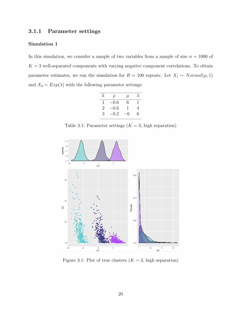
Simulation 1
In this simulation, we consider a sample of two variables from a sample of size n = 1000 of
K = 3 well-separated components with varying negative component correlations. To obtain
parameter estimates, we run the simulation for R = 100 repeats. Let X1 ∼ Normal(µ, 1)
and X2 ∼ Exp(λ) with the following parameter settings:
k ρ µ λ
1 −0.6 6 12 −0.6 1 43 −0.2 −6 6
Table 3.1: Parameter settings (K = 3, high separation)
Figure 3.1: Plot of true clusters (K = 3, high separation)
20
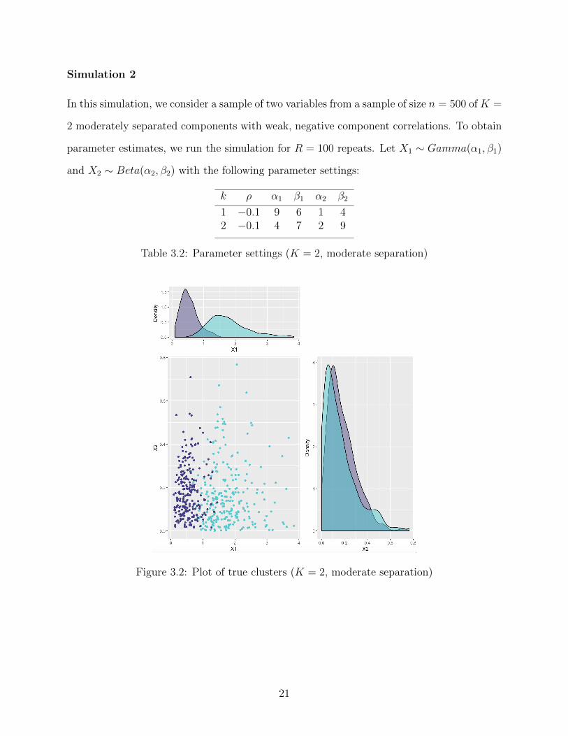
Simulation 2
In this simulation, we consider a sample of two variables from a sample of size n = 500 of K =
2 moderately separated components with weak, negative component correlations. To obtain
parameter estimates, we run the simulation for R = 100 repeats. Let X1 ∼ Gamma(α1, β1)
and X2 ∼ Beta(α2, β2) with the following parameter settings:
k ρ α1 β1 α2 β2
1 −0.1 9 6 1 42 −0.1 4 7 2 9
Table 3.2: Parameter settings (K = 2, moderate separation)
Figure 3.2: Plot of true clusters (K = 2, moderate separation)
21

Simulation 3
In this simulation, we consider a sample of three variables from a sample size of n = 1000 of
K = 3 mildly separated components with moderately strong, positve component correlations.
To obtain parameter estimates, we run the simulation for R = 50 repeats. Let X1 ∼
Gamma(α1, β1), X2 ∼ Normal(µ, 1) and X3 ∼ Beta(α3, β3) with the following parameter
settings:
k ρ12 ρ13 ρ23 α1 β1 µ α3 β3
1 0.5 0.5 0.5 8 4 0 10 12 0.5 0.5 0.5 5 8 −3 5 33 0.5 0.5 0.5 1 1 −2 7 5
Table 3.3: Parameter settings (K = 3, mild separation)
Figure 3.3: Plot of true clusters (K = 3, mild separation)
22

3.2 Model selection criterion
3.2.1 Bayesian information criterion
In cluster analysis, one challenge researchers face is the selection of the optimal number of
clusters given the data. This can be difficult in practice, especially when the clusters are
highly latent. Schwarz (1978) was one of the first to introduce the concept of model selection
using a Bayesian approach. The Bayesian Information Criterion (BIC) is widely used and,
as asserted by Franczak (2014), is shown to have advantageous asymptotic properties. The
BIC is defined as
BIC = −2`(x; Θ) + q log(n), (3.1)
where `(x; Θ) is the maximized log-likelihood, Θ is the MLE of Θ, q is the number of free
parameters and n is the sample size (Franczak, 2014). Thus, we select the optimal number of
components based on the model which minimizes the BIC. The BIC can be more conservative
than other model selection criterion as it penalizes both the number of free parameters in
the model as well as the sample size.
In this thesis, we use the BIC to identify the optimal number of clusters in the data. For
P variables and a mixture of K components, the number of free parameters, q, is calcualted
as
q = m+ (K − 1) +KP (P − 1)
2, (3.2)
where m is the number of marginal parameters needed to be estimated, (K−1) accounts for
the estimation of the mixing proportions, πk, and KP (P − 1)/2 accounts for the estimation
of K correlation matrices. Although the BIC is a popular means for model selection, the
number of components it selects may not necessarily be optimal (McNicholas, 2016), and a
deep comprehension of the subject matter is also highly valuable when choosing the number
23

of clusters.
3.2.2 Clustering indices
In order to assess the performance of GCDs in clustering data, we use a variety of clustering
indices to measure the similarity between groups (Desgraupes, 2017). In this section, we
outline three popular clustering indices: the Rand index, the Jaccard index and the Fowlkes-
Mallows index. These clustering indices lie in the interval [0, 1], where indices close to 1
indicate strong agreement of clustering and indices close to 0 indicate poor agreement of
clustering. Definitions obtained from Desgraupes (2017) and Ruan (2015) follow.
Let P1 represent partition 1 and P2 represent partition 2. For a pair of points, there are
four possibilities:
• the two points belong to the same cluster, according to both P1 and P2
• the two points belong to the same cluster according to P1, but not P2
• the two points belong to the same cluster according to P2, but not P1
• the two points do not belong to the same cluster, according to both P1 and P2
Denote A,B,C, and D the number of points belonging to each of the four categories,
respectively. We measure the similarity of the true cluster and computed cluster by counting
the number of pairs of points that are in A,B,C and D. Let n be the number of observations
and nt be the total number of pairs of points. Hence, we have
nt = A+B + C +D =n(n− 1)
2. (3.3)
Rand index
The Rand index is defined as
24

R =A+D
nt
, (3.4)
which measures the agreement of clustering by the proportion of pairs of points that belong
to the same cluster or do not belong to the same cluster, according to both P1 and P2.
Jaccard index
The Jaccard index is defined as
J =A
A+B + C, (3.5)
which measures the agreement of clustering by the proportion of pairs of points that belong
to the same cluster, according to both P1 and P2, relative to the number of pairs of points
that belong to the same cluster in at least one of the partitions.
Fowlkes-Mallows index
The Fowlkes-Mallows index is defined as
FM =A√
(A+B)(A+ C), (3.6)
which measures the agreement of clustering by the geometric mean of the proportion of
pairs of points that belong to the same cluster, according to both P1 and P2, relative to the
number of pairs of points that belong to the same cluster in at least one of the partitions.
In this chapter, we use these three clustering indices to measure the GCDs accuracy of
clustering. The adjustedRand function in the clues package (Chang et al., 2016) is used to
calculate these indices.
25
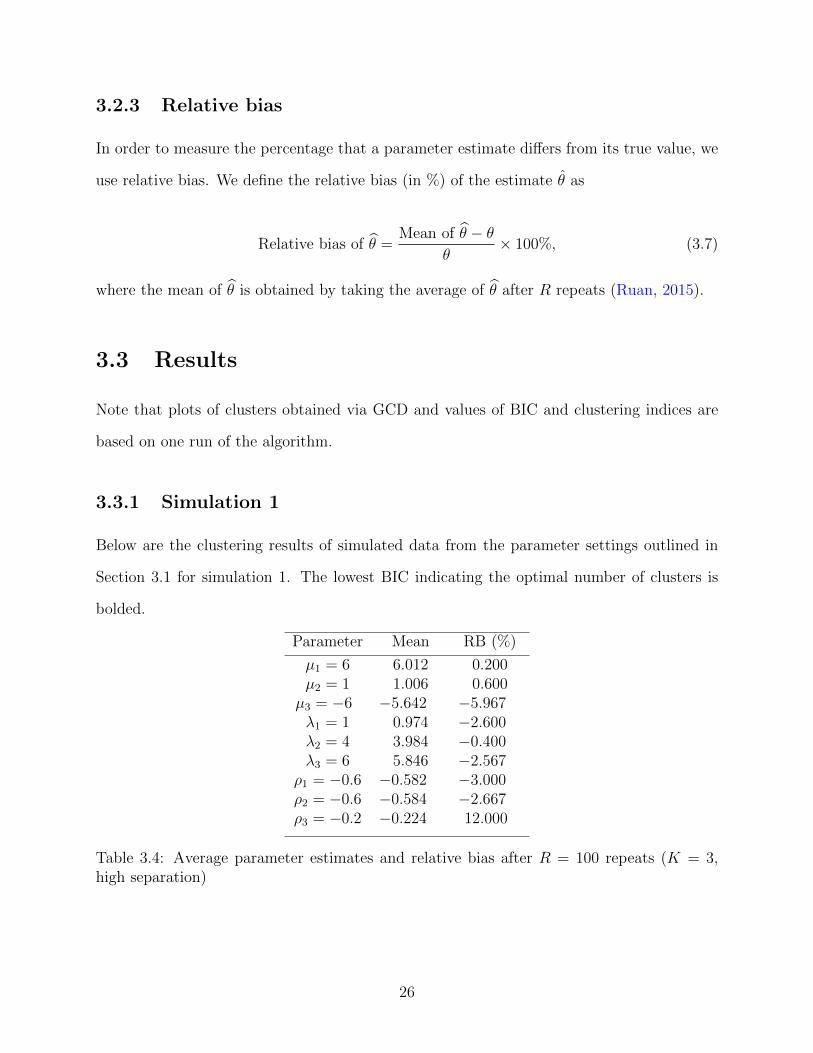
3.2.3 Relative bias
In order to measure the percentage that a parameter estimate differs from its true value, we
use relative bias. We define the relative bias (in %) of the estimate θ as
Relative bias of θ =Mean of θ − θ
θ× 100%, (3.7)
where the mean of θ is obtained by taking the average of θ after R repeats (Ruan, 2015).
3.3 Results
Note that plots of clusters obtained via GCD and values of BIC and clustering indices are
based on one run of the algorithm.
3.3.1 Simulation 1
Below are the clustering results of simulated data from the parameter settings outlined in
Section 3.1 for simulation 1. The lowest BIC indicating the optimal number of clusters is
bolded.
Parameter Mean RB (%)
µ1 = 6 6.012 0.200µ2 = 1 1.006 0.600µ3 = −6 −5.642 −5.967λ1 = 1 0.974 −2.600λ2 = 4 3.984 −0.400λ3 = 6 5.846 −2.567
ρ1 = −0.6 −0.582 −3.000ρ2 = −0.6 −0.584 −2.667ρ3 = −0.2 −0.224 12.000
Table 3.4: Average parameter estimates and relative bias after R = 100 repeats (K = 3,high separation)
26
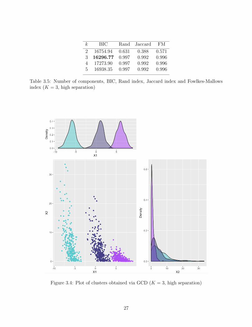
k BIC Rand Jaccard FM
2 16754.94 0.631 0.388 0.5713 16296.77 0.997 0.992 0.9964 17273.90 0.997 0.992 0.9965 16938.35 0.997 0.992 0.996
Table 3.5: Number of components, BIC, Rand index, Jaccard index and Fowlkes-Mallowsindex (K = 3, high separation)
Figure 3.4: Plot of clusters obtained via GCD (K = 3, high separation)
27
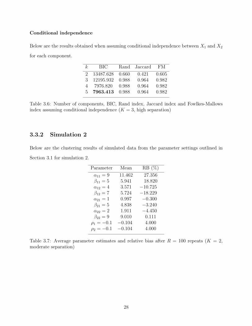
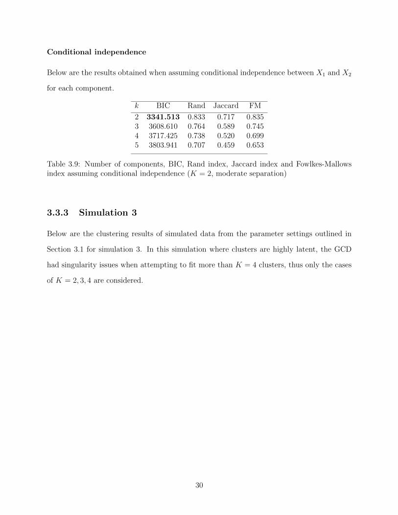
Conditional independence
Below are the results obtained when assuming conditional independence between X1 and X2
for each component.
k BIC Rand Jaccard FM
2 13487.628 0.660 0.421 0.6053 12195.932 0.988 0.964 0.9824 7976.820 0.988 0.964 0.9825 7963.413 0.988 0.964 0.982
Table 3.6: Number of components, BIC, Rand index, Jaccard index and Fowlkes-Mallowsindex assuming conditional independence (K = 3, high separation)
3.3.2 Simulation 2
Below are the clustering results of simulated data from the parameter settings outlined in
Section 3.1 for simulation 2.
Parameter Mean RB (%)
α11 = 9 11.462 27.356β11 = 5 5.941 18.820α12 = 4 3.571 −10.725β12 = 7 5.724 −18.229α21 = 1 0.997 −0.300β21 = 5 4.838 −3.240α22 = 2 1.911 −4.450β22 = 9 9.010 0.111ρ1 = −0.1 −0.104 4.000ρ2 = −0.1 −0.104 4.000
Table 3.7: Average parameter estimates and relative bias after R = 100 repeats (K = 2,moderate separation)
28
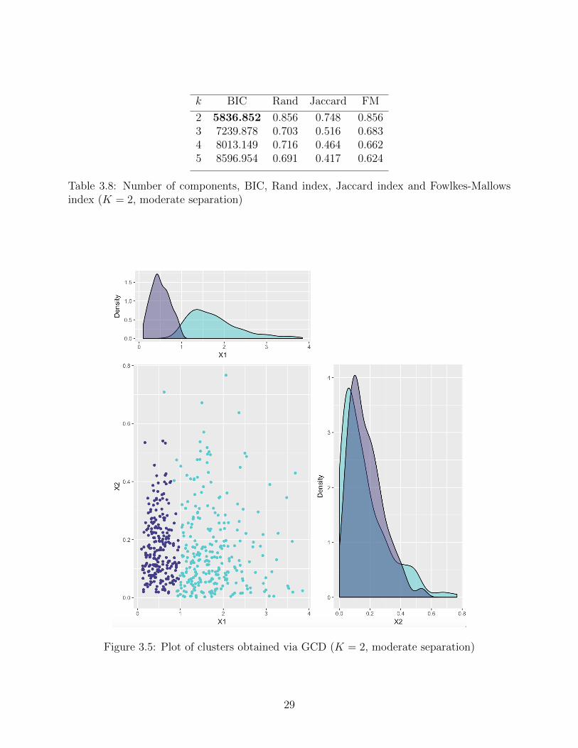
k BIC Rand Jaccard FM
2 5836.852 0.856 0.748 0.8563 7239.878 0.703 0.516 0.6834 8013.149 0.716 0.464 0.6625 8596.954 0.691 0.417 0.624
Table 3.8: Number of components, BIC, Rand index, Jaccard index and Fowlkes-Mallowsindex (K = 2, moderate separation)
Figure 3.5: Plot of clusters obtained via GCD (K = 2, moderate separation)
29
Conditional independence
Below are the results obtained when assuming conditional independence between X1 and X2
for each component.
k BIC Rand Jaccard FM
2 3341.513 0.833 0.717 0.8353 3608.610 0.764 0.589 0.7454 3717.425 0.738 0.520 0.6995 3803.941 0.707 0.459 0.653
Table 3.9: Number of components, BIC, Rand index, Jaccard index and Fowlkes-Mallowsindex assuming conditional independence (K = 2, moderate separation)
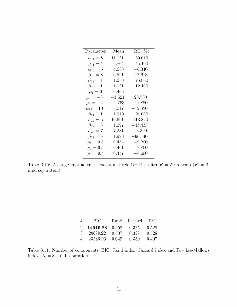
3.3.3 Simulation 3
Below are the clustering results of simulated data from the parameter settings outlined in
Section 3.1 for simulation 3. In this simulation where clusters are highly latent, the GCD
had singularity issues when attempting to fit more than K = 4 clusters, thus only the cases
of K = 2, 3, 4 are considered.
30
Parameter Mean RB (%)
α11 = 8 11.121 39.013β11 = 4 5.804 45.100α12 = 5 4.683 −6.340β12 = 8 6.591 −17.613α13 = 1 1.258 25.800β13 = 1 1.121 12.100µ1 = 0 0.406 −µ2 = −3 −3.621 20.700µ3 = −2 −1.763 −11.850α31 = 10 8.017 −19.830β31 = 1 1.910 91.000α32 = 5 10.691 113.820β32 = 3 1.697 −43.433α33 = 7 7.231 3.300β33 = 5 1.993 −60.140ρ1 = 0.5 0.454 −9.200ρ2 = 0.5 0.461 −7.800ρ3 = 0.5 0.457 −8.600
Table 3.10: Average parameter estimates and relative bias after R = 50 repeats (K = 3,mild separation)
k BIC Rand Jaccard FM
2 14910.88 0.459 0.325 0.5293 20688.22 0.537 0.338 0.5284 23236.26 0.649 0.330 0.497
Table 3.11: Number of components, BIC, Rand index, Jaccard index and Fowlkes-Mallowsindex (K = 3, mild separation)
31
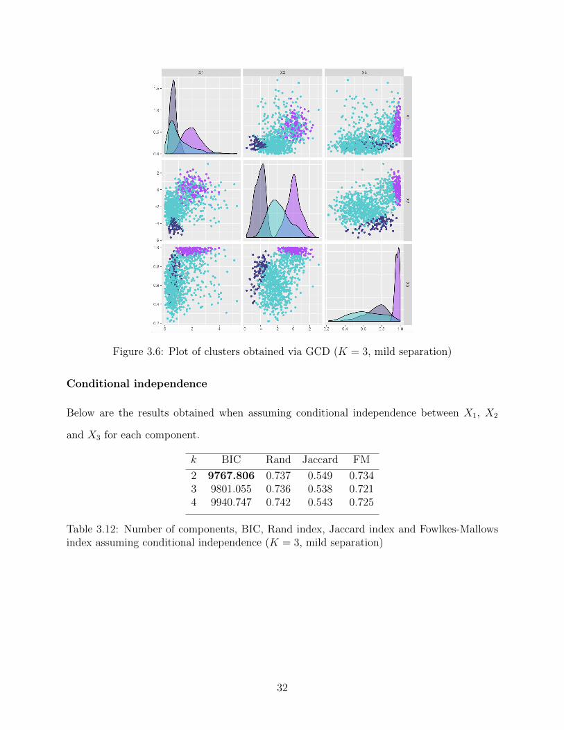
Figure 3.6: Plot of clusters obtained via GCD (K = 3, mild separation)
Conditional independence
Below are the results obtained when assuming conditional independence between X1, X2
and X3 for each component.
k BIC Rand Jaccard FM
2 9767.806 0.737 0.549 0.7343 9801.055 0.736 0.538 0.7214 9940.747 0.742 0.543 0.725
Table 3.12: Number of components, BIC, Rand index, Jaccard index and Fowlkes-Mallowsindex assuming conditional independence (K = 3, mild separation)
32
3.3.4 Discussion
In the case of K = 3 well-separated components, the GCD performs well and correctly
identifies the number of clusters. Clustering indices close to 1 reflect nearly perfect agreement
of clusters. The GCD is able to identify a maximum of K = 3 clusters, which is why the
clustering indices for the cases of K = 4 and K = 5 clusters are the same as K = 3, as
there were 0 observations assigned to the fourth and fifth component. After R = 100 repeats,
parameter estimates are close to their true values with relatively low bias. Additionally, under
the assumption of componentwise conditional independence, the GCD incorrectly selects the
number of clusters and has slightly lower clustering indices for K = 3 components.
For K = 2 moderately separated components, based on the BIC, the GCD correctly
selects the number of components. As expected, clustering indices are lower than the case
of well-separated components, but are still relatively close to 1. When assuming componen-
twise conditional independence, the GCD is able to identify the correct number of clusters.
However, in this case, clustering indices are slightly lower than when we take into account
the dependence between variables. After R = 100 repeats, parameter estimates are still
reasonably close to their true values, although with typically higher relative biases. Also,
since closed-form solutions for the MLEs of the marginal parameters do not exist, the use of
the multiroot function is more computationally intensive and is sometimes sensitive to the
initial values selected.
When considering the case of K = 3 components with mild separation, the GCD mis-
specifies the number of clusters and has much lower clustering indices than when there is
greater compenent separation. As a result of the mild component separation, parameter
estimates generally have higher bias and, due to computational tractability and efficiency,
we only consider R = 50 repeats. The high component latency also results in more singu-
larity issues and, in combination with the use of the multiroot function, results in much
slower calculations. Assuming conditional independence, we also have an incorrect selection
of components, but with higher clustering indices than when we do not make this assump-
33

tion. These results may be attributed to the fact that high component latency can lead to
an increased difficulty in identifying clusters and, consequently, their parameter estimates.
Overall, the GCD performs well in identifying the underlying structure of the data,
including parameter estimation and assigning cluster memberships. The GCD struggles
as the separation between clusters decreases, as this overlap makes it more challenging to
identify the true components, which is to be expected. From the simulation study, one may
also reasonably conclude that ignoring the componentwise dependence between variables
may yield misleading results.
In the next chapter, we apply this methodology to a dataset to further assess its perfor-
mance.
34
Chapter 4
Application
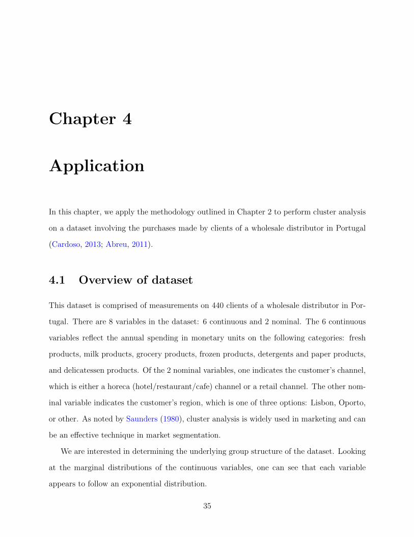
In this chapter, we apply the methodology outlined in Chapter 2 to perform cluster analysis
on a dataset involving the purchases made by clients of a wholesale distributor in Portugal
(Cardoso, 2013; Abreu, 2011).
4.1 Overview of dataset
This dataset is comprised of measurements on 440 clients of a wholesale distributor in Por-
tugal. There are 8 variables in the dataset: 6 continuous and 2 nominal. The 6 continuous
variables reflect the annual spending in monetary units on the following categories: fresh
products, milk products, grocery products, frozen products, detergents and paper products,
and delicatessen products. Of the 2 nominal variables, one indicates the customer’s channel,
which is either a horeca (hotel/restaurant/cafe) channel or a retail channel. The other nom-
inal variable indicates the customer’s region, which is one of three options: Lisbon, Oporto,
or other. As noted by Saunders (1980), cluster analysis is widely used in marketing and can
be an effective technique in market segmentation.
We are interested in determining the underlying group structure of the dataset. Looking
at the marginal distributions of the continuous variables, one can see that each variable
appears to follow an exponential distribution.
35
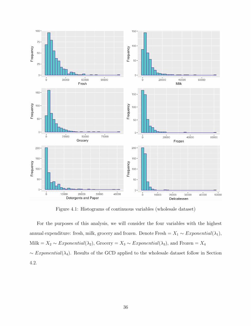
Figure 4.1: Histograms of continuous variables (wholesale dataset)
For the purposes of this analysis, we will consider the four variables with the highest
annual expenditure: fresh, milk, grocery and frozen. Denote Fresh = X1 ∼ Exponential(λ1),
Milk = X2 ∼ Exponential(λ2), Grocery = X3 ∼ Exponential(λ3), and Frozen = X4
∼ Exponential(λ4). Results of the GCD applied to the wholesale dataset follow in Section
4.2.
36
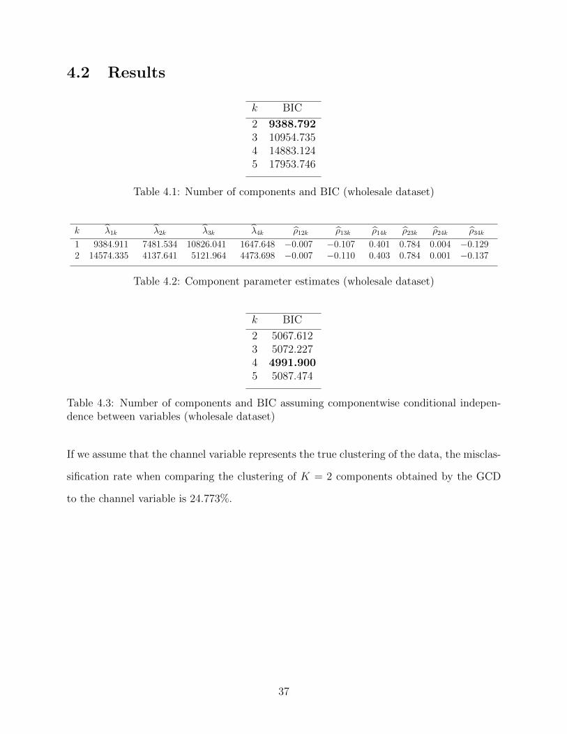
4.2 Results
k BIC
2 9388.7923 10954.7354 14883.1245 17953.746
Table 4.1: Number of components and BIC (wholesale dataset)
k λ1k λ2k λ3k λ4k ρ12k ρ13k ρ14k ρ23k ρ24k ρ34k
1 9384.911 7481.534 10826.041 1647.648 −0.007 −0.107 0.401 0.784 0.004 −0.1292 14574.335 4137.641 5121.964 4473.698 −0.007 −0.110 0.403 0.784 0.001 −0.137
Table 4.2: Component parameter estimates (wholesale dataset)
k BIC
2 5067.6123 5072.2274 4991.9005 5087.474
Table 4.3: Number of components and BIC assuming componentwise conditional indepen-dence between variables (wholesale dataset)
If we assume that the channel variable represents the true clustering of the data, the misclas-
sification rate when comparing the clustering of K = 2 components obtained by the GCD
to the channel variable is 24.773%.
37
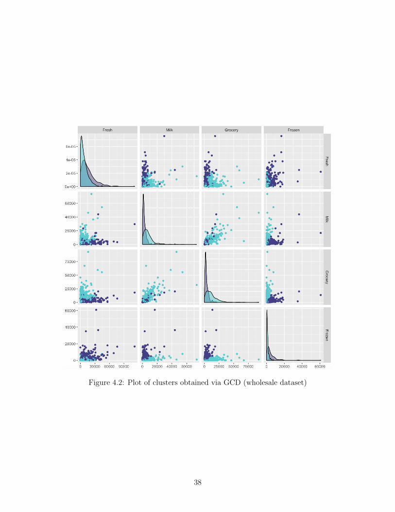
Figure 4.2: Plot of clusters obtained via GCD (wholesale dataset)
38
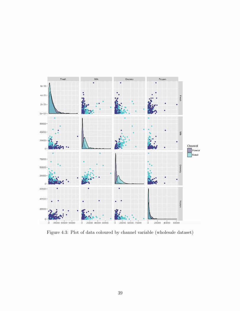
Figure 4.3: Plot of data coloured by channel variable (wholesale dataset)
39

4.3 Discussion
The GCD selects K = 2 as the optimal number of clusters, which agrees with the fact that
there are two types of customer channels. Comparing the clusters obtained via the GCD
with the grouping from the channel variable, the GCD performs well in identifying the group
structure of the data with a relatively low misclassification rate considering the latency of
the clusters.
Furthermore, when assuming componentwise conditional independence between the vari-
ables, the GCD selects K = 4 components as the optimal number of clusters, which do
not have a straightforward explanation in the context of this data. This demonstrates the
potential issues that may arise when the dependence structure of the data is ignored.
40
Chapter 5
Conclusion
In this chapter, we summarize the thesis and provide a discussion of its results, as well as
consider possible related future work.
5.1 Summary
This thesis explores the use of a hybrid approach to cluster analysis of correlated non-
Gaussian continuous data via GCDs. GCDs provide us with a flexible way to model the
joint distribution of a variety of non-Gaussian continuous data, while not relying on the
assumption of conditional independence between variables.
We adopt a methodology that combines the approaches of IFM and the PX-EM algo-
rithm. The use of IFM enables us to maximize marginal parameter estimates separately,
while still maximizing the correlation between normal scores jointly (Joe and Xu, 1996).
This increases the computational efficiency of the algorithm and still allows us to account
for the relationship between variables. Having a constrained parameter space poses addi-
tional challenges for parameter estimation, but adopting the PX-EM algorithm allows us to
overcome these convergence issues, while preserving the desirable properties of the ordinary
EM algorithm (Liu et al., 1998).
Simulations were performed to evaluate the performance of GCDs in clustering disparate
41
continuous data. From these simulations, we can see that, overall, the GCD performs well
in identifying components and obtaining parameter estimates. Furthermore, these simula-
tions highlight the potential issues that may arise when assuming conditional independence
between variables. When closed-form expressions for MLEs of marginal parameters are not
available, the use of the multiroot function may decrease the computational efficiency of
the algorithm. Also, this function is dependent on initial values, and poor selection of these
initial values may lead to slower convergence rates or even non-convergence. As expected,
when component latency is increased, the GCD does not perform as well. Ultimately, GCDs
appear to be a useful tool in the cluster analysis of non-Gaussian continuous data.
To demonstrate the potential applications of our methodology, we apply the GCD to a
dataset on the client’s of a wholesale distributor. The GCD identifies K = 2 clusters from
the data that could correspond to the customer channel variable. Comparing the clustering
we obtain to the grouping from the channel variable, the GCD does well in identifying the
underlying structure of the data. Moreover, when assuming conditional independence, the
GCD selects K = 4 clusters, which does not have an obvious interpretation for this dataset.
5.2 Future work
A natural extension of this work would be to consider the case of mixed data; that is, data
comprised of both continuous and discrete variables. Extending our methodology to the
mixed data setting could be useful in a variety of statistical settings. See Jiryaie et al.
(2016) for a comprehensive review of GCDs for mixed data.
One could also consider the use of a different copula with which to join together the
margins. For example, one could adopt a class of t copulas. As noted by Demarta and McNeil
(2007), a t copula may be able to capture more heterogeneity and extreme observations in
the data. There are a variety of copulas one could select, depending on the nature of the
data and how one wishes to model the dependence between variables.
42
Bibliography
Abreu, N. (2011). Analise do perfil do cliente Recheio e desenvolvimento de um sistema
promocional. Mestrado em Marketing, ISCTE-IUL, Lisbon.
Andrews, J. L. and McNicholas, P. D. (2012). Model-based clustering, classification, and dis-
criminant analysis via mixtures of multivariate t-distributions. Statistics and Computing,
22(5):1021–1029.
Cardoso, M. (2013). Wholesale customers data set. http://archive.ics.uci.edu/ml/
datasets/Wholesale+customers#.
Chang, F., Qiu, W., Carey, V., Zamar, R., Lazarus, R., and Wang, X. (2016). Package
‘clues’. https://cran.r-project.org/web/packages/clues/clues.pdf.
Dawid, A. (1979). Conditional independence in statistical theory. Journal of the Royal
Statistical Society. Series B (Methodological), 41(1):1–31.
Demarta, S. and McNeil, A. (2007). The t copula and related copulas. International Statis-
tical Review, 73(1):111–129.
Dempster, A., Laird, N., and Rubin, D. (1977). Maximum likelihood from incomplete data
via the EM algorithm. Journal of the Royal Statistical Society. Series B (Methodological),
39(1):1–38.
Desgraupes, B. (2017). Clustering indices. University Paris Ouest, Lab Modal’X.
43
Everitt, B., Landau, S., Leese, M., and Stahl, D. (2011). Cluster Analysis. Wiley, 5th ed.
Franczak, B. (2014). Mixtures of shifted asymmetric Laplace distributions. Doctoral Thesis,
University of Guelph.
Jiryaie, F., Withanage, N., Wu, B., and de Leon, A. (2016). Gaussian copula distributions
for mixed data, with application in discrimination. Journal of Statistical Computation and
Simulation, 86(9):1643–1659.
Joe, H. and Xu, J. (1996). The estimation method of inference functions for margins for
multivariate models. UBC Faculty Research and Publications.
Kosmidis, I. and Karlis, D. (2016). Model-based clustering using copulas with applications.
Statistics and Computing, 26(5):1079–1099.
Liu, C., Rubin, D., and Wu, Y. (1998). Parameter expansion to accelerate EM: the PX-EM
algorithm. Biometrika, 85(4):755–770.
McLachlan, G. and Krishnan, T. (2008). The EM Algorithm and Extensions. Wiley, 2nd ed.
McNicholas, P. (2016). Model-based clustering. Journal of Classification, 33(3):331–373.
Nelsen, R. (2006). An Introduction to Copulas. Springer.
Ren, M. (2016). Likelihood analysis of Gaussian copula distributions for mixed data via a
parameter-expanded Monte Carlo EM (PX-MCEM) algorithm. Master’s Thesis, Univer-
sity of Calgary.
Ruan, J. (2015). Cluster analysis of gene expression profiles via flexible count models for
RNA-seq data. Master’s Thesis, University of Calgary.
Saunders, J. (1980). Cluster analysis for market segmentation. European Journal of Mar-
keting, 14(7):422–435.
44

Schwarz, G. (1978). Estimating the dimension of a model. The Annals of Statistics, 6(2):461–
464.
Soetaert, K. (2015). Package ‘rootSolve’. https://cran.r-project.org/web/packages/
rootSolve/vignettes/rootSolve.pdf.
Wu, B. (2013). Contributions to copula modeling of mixed discrete-continuous outcomes.
Doctoral Thesis, University of Calgary.
Xu, H. and Craig, B. (2010). Likelihood analysis of multivariate probit models using a
parameter expanded MCEM algorithm. Technometrics, 52(3):340–348.
45


