Closed form stiffness matrices and error estimators for plane hierarchic triangular elements

INTERNATIONAL JOURNAL FOR NUMERICAL METHODS IN ENGINEERING, VOL. 31, 879-894 (1991)

CLOSED FORM STIFFNESS MATRICES AND ERROR ESTIMATORS FOR PLANE HIERARCHIC TRIANGULAR

ELEMENTS

KENT L. LAWRENCE,' RAIN v. NAMBIAR' AND BRAD BERGMANN:

Department of Mechanical Engineering, University of Texas at Arlington, Arlington TX 76019, U.S.A.

SUMMARY Closed form expressions for the stiffness matrix and a simple error estimator and error indicator are derived for plane straight sided triangular finite elements in elasticity problems. The calculation of the error estimator is performed on an element by element basis, and is found to be very accurate and efficient. In general, the solutions for benchmark problems using the error indicators for selective refinement of the regions show accelerated convergence when compared to the convergence rate of solutions using uniform mesh refinement. Evaluation of the stiffness matrices and error estimators using explicit formulations is found to be several times faster than numerical integration.

INTRODUCTION

Closed form representations of element stiffness matrices may be preferred if they offer significant improvements in computational efficiency and accuracy when compared with other procedures. Efficient element formulation is particularly important in adaptive problems where many meshes may be generated and solved in the course of a specific problem solution. Triangular elements have a complete polynomial basis and therefore offer certain advantages over quadrilateral elements which employ incomplete polynomials. Zienkiewicz et a!.,' Cook' and Dow and Byrd3 have discussed the inherent difficulty presented by the incomplete polynomials used in quadrilateral elements. Triangular elements also play an important role in adaptive finite element analysis and Shephard'.' has observed that triangles may be better suited for use with general purpose mesh generation schemes than quadrilateral elements. In addition, the advantages to be gained from using the hierarchic formulation are well known and have been discussed in by Zienkiewicz et aL9 and Szabo et a!.''

The above observations suggest the need for a family of more efficient triangular elements employing the hierarchic formulation. Tinawi" and Subramaniam and Base'* have demon- strated the use of closed form integration in the formulation of the stiffness matrix for non- hierarchic triangular elements. The work presented here demonstrates that stiffness matrices and error estimators for hierarchic straight edged triangular elements can also be obtained in closed form.

The estimation of the error in finite element stress analysis is often accomplished by using the fact that a uniform h-version or p-version mesh will eventually converge to the exact solution at a

* Professor Graduate Research Assistant

0029-598 1/91/050879-16$08.00 0 1991 by John Wiley & Sons, Ltd.

Received 14 November 1989 Revised 15 June 1990

880 K. L. LAWRENCE. R. V. NAMBIAR AND 8. BERGMANN

uniform logarithmic rate as the number of degrees of freedom is increased. This procedure requires three solutions that lie in the asymptotic range. An estimate of the ‘true’ solution can then be found.13*14 This method suffers from the fact that a uniform mesh reduction (or p-level increase) is assumed, but if this assumption is correct the convergence is usually very slow; however, if the assumption is not correct the estimate will naturally be poor.

The rates of convergence of the h- and the p-method have been established by Babuska and Szabo.” Babuska and Dorr16 showed that faster convergence could be obtained using an h-p method that uses an a priori analysis to optimally refine the mesh. Early efforts at error estimation and adaptive mesh refinement were made using the strain energy of the element as an indicator. Szabo and Dunavant” have shown that the element strain energy is a poor error indicator for selecting elements whose p-level is to be increased in order to obtain rapid convergence. The error inherent in the finite element solution has two parts;18 the first part is proportional to the error in the second derivatives of the displacement within the element and is attributed to the fact that the solution satisfies the continuity equation only in an integral sense and not at every point in the domain. The second, and usually the more dominant part of the error for low p-level elements, is caused by discontinuities in the first derivatives of the displacement at the boundaries of the element, since only displacement continuity is enforced across inter-element boundaries. A number of error indicators have been proposed that include the contributions of both these sources of error.

Babuska and Rhienboldt” suggested the use of norms based on the residual forces over the domain. Kelly20~2’ and Kelly and Isles22 proposed the partitioning of a set of fictitious residual ‘error forces’ between the elements followed by a complementary analysis to solve for the error, and have shown that an upper bound for the error in strain energy could be obtained. The difficulty with the methods that include the residual has been the fact that they are very complex, and as a result, the calculation Qf the indicator involves a very large numerical computation effort.

Zienkiewicz and Z ~ U ~ ~ proposed a simple and computationally efficient error estimator in the energy norm by obtaining a smoothed solution that is a better approximation of the stress distribution than the stress distribution obtained from the finite element solution. The difference between these solutions is used to obtain an estimate of the error. Zienkiewicz and Z ~ U ~ ~ have also employed this method successfully for the analysis of the plate bending problem and a similar approach has been used by Jirousek and Venkate~h.’~ Byrd26 has implemented this method in the development of several similar indicators for which the improved solution is obtained by employing various local smoothing assumptions. The closed form error estimator and error indicator presented here are based on the method that employs local nodal stress averaging as used by Byrd.

THE ELEMENT FORMULATION

The area or natural co-ordinates L , , L, and L3 of any point inside a triangle are related by2’

L , + L , + L3 = 1 ( 2 ) In the assumed displacement formulation of the stiffness matrices, the displacement (u, u ) at any point within the element is given in terms of the nodal displacement vectors 6u and 6v by

CLOSED FORM STIFFNESS MATRICES 881

where N is the shape function in terms of the area co-ordinates. The three node CST element, for example, has a shape function

N = C L , L, L31 (4) where each term in N corresponds to the displacement of a triangle vertex. The hierarchic LST element belonging to the hierarchic family of triangular elements described by Babuska et aL2* has a shape function given by

N = [ L , L2 L3 2LiL2 2L2L3 2LSL1] (5 )

Using (2) to eliminate L 3 , the shape functions may be written as functions of L , and L, alone in the form

N = STQ (6) where Q is a square matrix of order r that contains constant coefficient terms. P e a n ~ ~ ~ has shown that the r entries of the vector S are of the form LTL; and together form a linearly independent set that spans the space of polynomials of order p , where

r = (P + 2)(P + 1) /2 (7)

S=[1 L , L , L: L , L , L ; ] (8)

The vector S for the LST element is

The expression for the strain E is given by

1 0 0 0 au au au av

0 1 1 0 (9)

The global co-ordinates of any point in the element are given in terms of the element area co- ordinates by

CX Y I = C L i L2 L3I [ ;; ;;I (10)

We use (2) to represent L3 in terms of L , and L , and, upon differentiation, we get the inverse of the Jacobian

Y 2 3 Y31 1 where x i j = xi - xj, and J is the determinant of the Jacobian, which is twice the area of the triangle, and is given by

= x 1 3 Y 2 3 - x 3 2 Y 3 1

The derivatives of the displacements in global and local co-ordinates are related by

[ au au a~ a , ] = - [r 0 1 g

ax ay ax ay o r _ - - - -

882

where

K. L. LAWRENCE, R. V. NAMBIAR AND B. BERGMANN

We differentiate the expressions for u and u in (3) to get

L J

where R is a matrix of derivatives of the shape functions,

where

Thus, the strain can be written as

E = PR[ E]

The strain energy U is given by

where D is the elasticity matrix. Substituting for E using (15) and changing the variables of integration to natural co-ordinates, we get

u = jol jol-"' gTPTDPgtJdLldL2

where t is the thickness of the element. Substituting for g using (13) and setting G = P'DP, we get

1 U = -[6uT 2 6vT] [K] [t]

where [K] is the element stiffness matrix, and for an element of uniform thickness,

[K] = t J 1; { I - L z RTGRdL,dL,

Note that G is a square matrix of order 4, which depends only on the triangle geometry and the material constants, and is independent of the order of the element, and R is a matrix of polynomials in L , and L,. Substituting for R using (14) and integrating using the formula

p ! q! LI;L4,dLldL -

- ( p + q + 2)!

CLOSED FORM STIFFNESS MATRICES

we obtain the stiffness matrix in the form

xx XY [ K 1 = t J [ XYT

where

where -01, B and V are matrices of constants

d' = Q T d * Q

LB = QTLB*Q

%? = QT%?*Q

and

883

(22)

The matrices d*, B* and %* are calculated using (21) since the matrix S and its derivatives contain only polynomials in L, and L,.

here

( i , - j,)( in - j,)( i, + in - j , - j , - 2)! (j, + j , ) ! ( i n - j d !

a?:,, = -

a;,, =

%?;,n = ~~

( i m - j m ) j n ( i m + i n - j m - j n - l ) ! ( j , , , + j , - l ) ! ( i n - j n Y

j , j , ( i , + in - j , - j , ) ! ( j , + j , - 2 ) ! ( i n - j A !

irn(irn - 1 ) . m = + J m + 1 2

Thus, using (22)-(26), we can obtain the stiffness matrix in closed form.

884 K. L. LAWRENCE. R. V. NAMBIAR AND B. BERGMANN

THE ERROR ESTIMATOR

Since the finite element procedure is based on minimizing the total potential energy, an error estimate in the energy norm is the most natural one to use. The error in the energy norm for an element is

I r _.__

where e, is the error in the calculated stress and C is the material compliance matrix. If the stress distribution from a finite element method solution is examined, it will be seen that a node shared by two elements will usually have two different stress values. This is because, although displacement continuity is guaranteed across inter-element boundaries, strain continuity is not enforced. It is then reasonable to assume that in problems involving a single material, the actual stress at the node would lie somewhere between the values calculated from each element; so an improved estimate of the stress distribution can be obtained by finding a smoothed stress solution c*. An approximation for the error in the stress is obtained from the difference between this improved solution and the finite element solution by

e u = o * - 6 (28) where C is the stress distribution obtained directly from the finite element solution. Zienkiewicz and ZhuZ3 have shown that the smoothed solution cr* is in fact a more accurate representation of the stress distribution than 6. The mathematical analysis of this estimator is provided in Reference 30. The solution, however, requires the inversion of a large, problem dependent matrix whose order is the same as the number of degrees in the problem and accomplished by using an efficient iterative scheme. Byrd26 has shown for benchmark problems that indicators that use averaged nodal stresses (NAl), so that smoothing is done on a local basis, are comparable in accuracy to the globally smoothed Zienkiewicz-Zhu error indicator.

Byrd observed that an improved solution that is smoothed on a local basis can also be obtained by averaging the stresses at each node, using nodal stresses calculated for each element associated with the node. The stress are interpolated over the element rather than globally using the element shape function N,

G * = 0 N 0 ii* [: : t ] where the averaged nodal stress is given by

a:

c :y

ii* = [ and is calculated by simple averaging of the stress in each element associated with a given node. For example, in the case of the CST element, this is equivalent to interpolating a linear stress distribution over the element using the averaged stresses. In case of higher order elements, it is not necessary to use the same shape functions that were used to calculate the stiffness matrix for interpolating the stresses. Care must be taken, however, if the mid-side and internal shape functions chosen do not correspond to nodal displacements, as is the case in hierarchic elements.


The appropriate function of the derivatives of the smoothed stresses will then have to be calculated at the internal and mid-side nodes.

The element error estimator is thus obtained from (27),

l l e i ~ ~ 2 = 6 ( . . - i ) T C ( ~ * - i ) d Q (31)

and expanding,

11 ei 11 = ja a* Ca* dQ - 2 In a*T Cij dQ + ja iT C i dQ (32)

The first term and last terms are twice the strain energy as calculated from the smoothed stress solution and from the finite element method solution, and the middle term corresponds to the coupling between the two stress distributions. All three terms may be obtained in closed form for plane triangular elements. The finite element method solution stress distribution is obtained from

i = D & (33) The first term can be written in the form

c, ,w c,,w c,3w c l l w c12w c 1 3 w

c31w c32w c33w

and the second term can be written as

a * T

where

(34)

(35)

The matrices W, X and Y are easily calculated using (21) since the shape matrix N and its derivatives contain only polynomials in L , and L,. The matrices W, X and Y are calculated in advance and stored in the program code. The last term in (32) is obtained from the stiffness matrix and nodal displacements and is twice the energy of the finite element solution,

Thus the error in the energy norm for each element can be calculated readily in closed form using expressions (34), (35) and (37). The energy norm for the entire finite element model is obtained by

II 6 II = C II Gi I I (38)


and error in energy norm from

II e II ' = 1 II ei II

11412 = I I i 1 I 2 + Ilel12

The corrected energy norm is

and the error estimator is calculated from

II e II q = - II u II

The calculation of an element refinement ratio also follows Zienkiewicz and Z ~ U . ' ~ If a maximum permissible error fraction f i is specified for the solution, a mean permissible error for an element can be calculated from

where rn is the number of elements. The refinement ratio ti is obtained for each element,

All elements for which t i > 1 must be subdivided to the extent specified by the magnitude of t i and the analysis repeated. If the actual error 11 e I( for the solution for benchmark problems can be calculated, an estimate of the effectivity of the indicator 0 can be obtained comparing the predicted error in the solution to the actual error achieved,

RESULTS

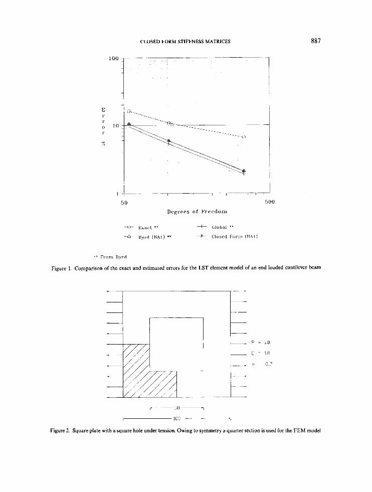
The closed form stiffness matrix and error estimator expressions discussed above have been employed to solve several evaluation problems and the results are given below. Figure 1 compares Byrd's results26 found from a series of uniform mesh models for an end loaded cantilever beam with length to breadth ratio of 10.0 with the error estimates calculated using the closed form expressions for the hierarchic LST element. Byrd has suggested that the error is always underestimated, and the calculated estimates bear this out. Zienkiewicz and Z ~ U ~ ~ suggested multiplying by empirical factors of 1.3 for CST elements and 1.4 for LST elements, so as to obtain a more accurate estimate of the error. These empirical factors were not found to improve the error estimates consistently for the locally smoothed method.

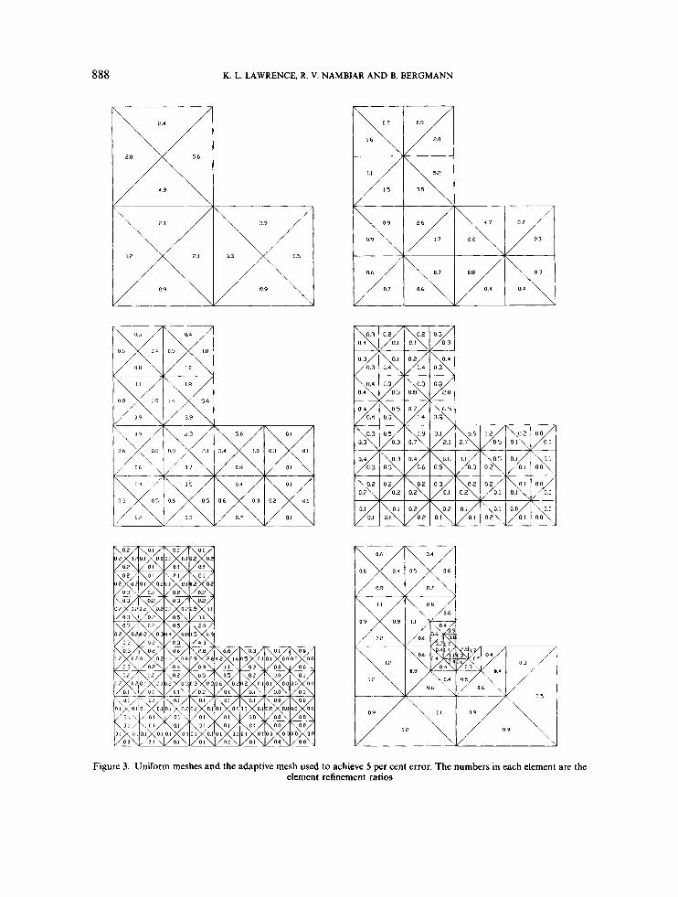
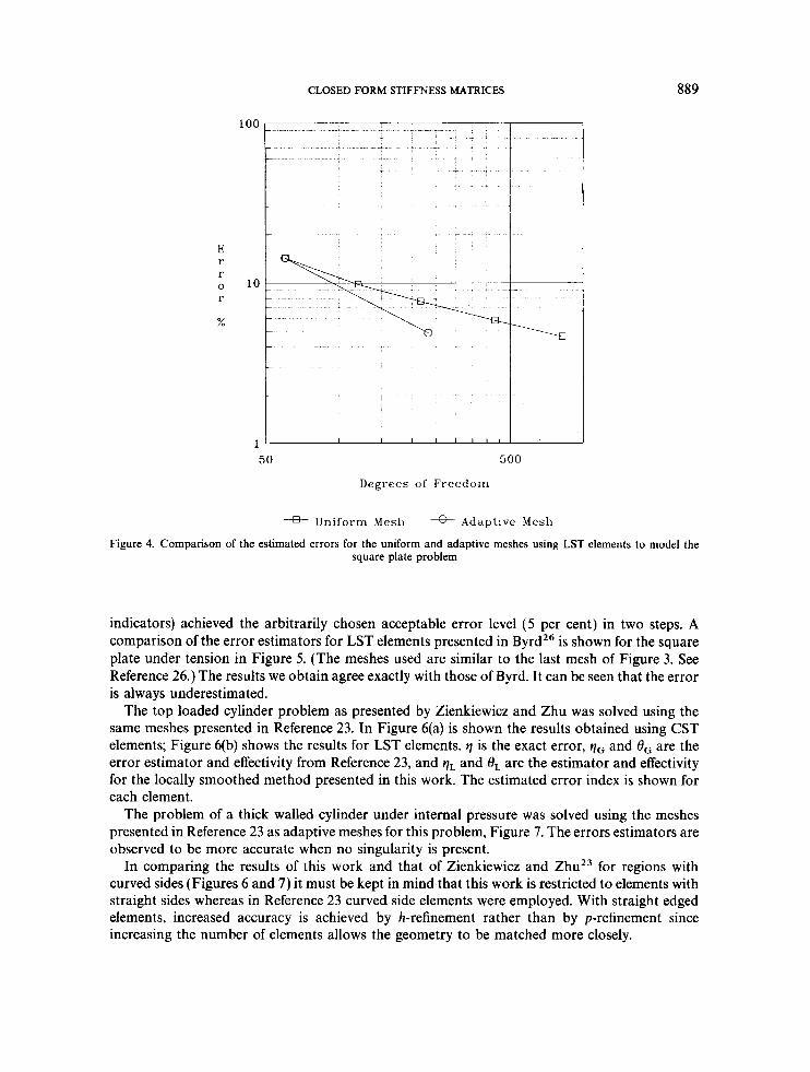
The problem of a square plate with a square hole is shown in Figure 2. A singularity occurs at the re-entrant corner. Figure 3 shows a series of meshes obtained by uniform element size reduction along with the adaptive mesh obtained using the error indicators of the coarsest uniform mesh. The numbers within each element is ti the refinement ratio. The LST model solution error is shown in Figure 4 as a function of the number of degrees of freedom for the meshes considered. This indicates that the solution converges faster when the mesh refinement is done adaptively using the error indicator rather than using uniform mesh refinement. In the case shown, the adaptive remeshing (including the empirical multiplying factor of 1-4 for the error


1 ____ 1 - 1 - I - - - - r - 7 1 1

500 c 50

Degrees of Freedom

* * I+om Uyrd

Figure 1. Comparison of the exact and estimated errors for the LST element model of an end loaded cantilever beam

50 -,

100

Figure 2. Square plate with a square hole under tension. Owing to symmetry a quarter section is used for the FEM model

888 K. L. LAWRENCE, R . V. NAMBIAR A N D B. BERGMANN

Figure 3. Uniform meshes and the adaptive mesh used to achieve 5 per cent error. The numbers in each element are the element refinement ratios


l o o r

10

1 50 500

Degrees of Freedoin

-ff Uniform Mesh ++ Adaptive Mesh

Figure 4. Comparison of the estimated errors for the uniform and adaptive meshes using LST elements to model the square plate problem

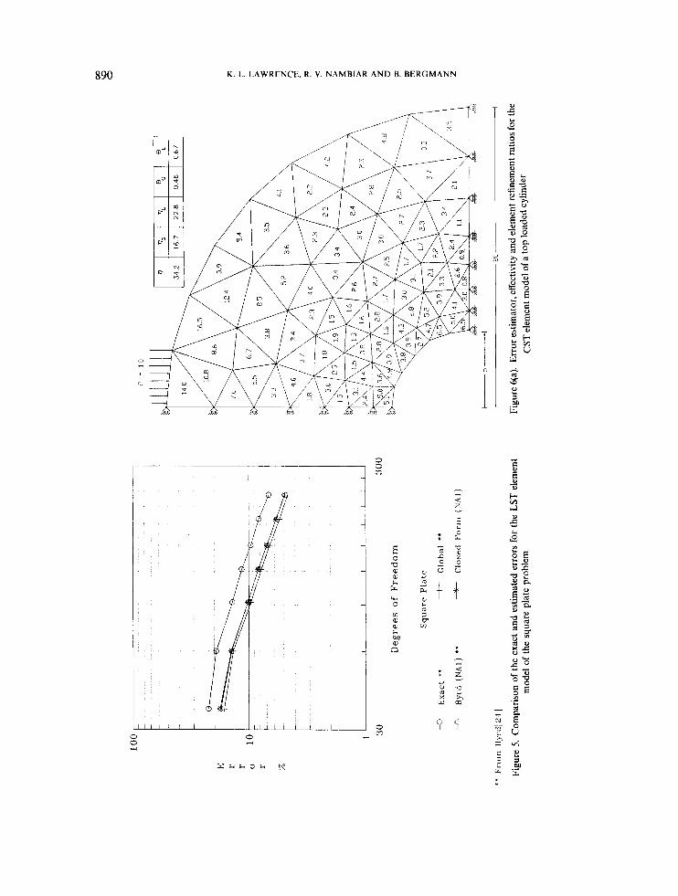
indicators) achieved the arbitrarily chosen acceptable error level (5 per cent) in two steps. A comparison of the error estimators for LST elements presented in ByrdZ6 is shown for the square plate under tension in Figure 5. (The meshes used are similar to the last mesh of Figure 3. See Reference 26.) The results we obtain agree exactly with those of Byrd. It can be seen that the error is always underestimated.

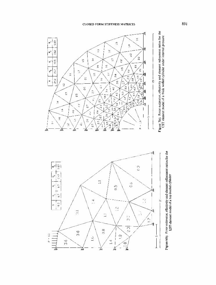
The top loaded cylinder problem as presented by Zienkiewicz and Zhu was solved using the same meshes presented in Reference 23. In Figure 6(a) is shown the results obtained using CST elements; Figure 6(b) shows the results for LST elements. q is the exact error, q, and 8, are the error estimator and effectivity from Reference 23, and qL and OL are the estimator and effectivity for the locally smoothed method presented in this work. The estimated error index is shown for each element.

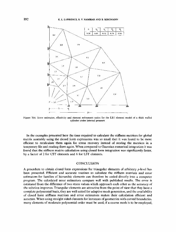
The problem of a thick walled cylinder under internal pressure was solved using the meshes presented in Reference 23 as adaptive meshes for this problem, Figure 7. The errors estimators are observed to be more accurate when no singularity is present.

In comparing the results of this work and that of Zienkiewicz and Z ~ U ~ ~ for regions with curved sides (Figures 6 and 7) it must be kept in mind that this work is restricted to elements with straight sides whereas in Reference 23 curved side elements were employed. With straight edged elements, increased accuracy is achieved by h-refinement rather than by p-refinement since increasing the number of elements allows the geometry to be matched more closely.

loo

i

10

t I

I I

I I

Il

l

1'

30

300

Deg

rees

of

Fre

edo

m

Sq

uar

e P

late

Ex

act

**

Glo

bal

**

*

~y

~d

(N

AI)

**

+++ C

lose

d F

orm

(N

AI)

P =

1.0

P r r

** F

rom

Hyr

d[24

]

Figu

re 5

. C

ompa

rison

of

the

exac

t and

est

imat

ed e

rror

s fo

r th

e LS

T el

emen

t m

odel

of

the

squa

re p

late

pro

blem

+5+

20 -

Figu

re 6

(a).

Err

or e

stim

ator

, eff

ectiv

ity an

d el

emen

t ref

inem

ent r

atio

s for

the

CST

elem

ent m

odel

of a

top

load

ed c

ylin

der


1 5 1 r 20 -

Figure 7(b). Error estimator, effectivity and element refinement ratios for the LST element model of a thick walled cylinder under internal pressure

In the examples presented here the time required to calculate the stiffness matrices for global matrix assembly using the closed form expressions was so small that it was found to be more efficient to recalculate them again for stress recovery instead of storing the matrices in a temporary file and reading them again. When compared to Gaussian numerical integration it was found that the stiffness matrix calculation using closed form integration was significantly faster, by a factor of 2 for CST elements and 6 for LST elements.

CONCLUSION

A procedure to obtain closed form expressions for triangular elements of arbitrary p-level has been presented. Efficient and accurate routines to calculate the stiffness matrices and error estimates for families of hierarchic elements can therefore be coded directly into a computer program. The calculated error estimators compare well with published results. The error is estimated from the difference of two stress values which approach each other as the accuracy of the solution improves. Triangular elements are attractive from the point of view that they have a complete polynomial basis, they are well suited for adaptive mesh generation, and the availability of closed form stiffness matrices and error estimators makes their calculation efficient and accurate. When using straight sided elements for instances of geometries with curved boundaries, many elements of moderate polynomial order must be used; if a coarse mesh is to be employed,


1 5 1 r 20 -

Figure 7(b). Error estimator, effectivity and element refinement ratios for the LST element model of a thick walled cylinder under internal pressure

In the examples presented here the time required to calculate the stiffness matrices for global matrix assembly using the closed form expressions was so small that it was found to be more efficient to recalculate them again for stress recovery instead of storing the matrices in a temporary file and reading them again. When compared to Gaussian numerical integration it was found that the stiffness matrix calculation using closed form integration was significantly faster, by a factor of 2 for CST elements and 6 for LST elements.

CONCLUSION

A procedure to obtain closed form expressions for triangular elements of arbitrary p-level has been presented. Efficient and accurate routines to calculate the stiffness matrices and error estimates for families of hierarchic elements can therefore be coded directly into a computer program. The calculated error estimators compare well with published results. The error is estimated from the difference of two stress values which approach each other as the accuracy of the solution improves. Triangular elements are attractive from the point of view that they have a complete polynomial basis, they are well suited for adaptive mesh generation, and the availability of closed form stiffness matrices and error estimators makes their calculation efficient and accurate. When using straight sided elements for instances of geometries with curved boundaries, many elements of moderate polynomial order must be used; if a coarse mesh is to be employed,


curved sided elements of high polynomial order must be developed separately by numerical integration, for use at the curved boundaries.

ACKNOWLEDGEMENT

The authors wish to thank the reviewers for their helpful comments.

REFERENCES

I . 0. C. Zienkiewicz, R. L. Taylor and J. M. Too, ‘Reduced integration techniques in general analysis of plates and

2. R. D. Cook, ‘Avoidance of parasitic shear in plane element’, J . Struct. Diu. ASCE, 1239-1253 (1975). 3. J. 0. Dow and D. E. Byrd, ‘The identification and elimination of artificial stiffening errors in finite elements’, Int . j.

4. J. Peraire, M. Vahdati, K. Morgan and 0. C. Zienkiewicz, ‘Adaptive remeshing for compressible flow computations’,

5. 0. C. Zienkiewicz, J. Z. Zhu and N. G. Gong, ‘Effective adaptive h-p procedures for practical engineering analysis’,

6. P. Roberti and M. A. Melkanoff, ‘Self-adaptive stress analysis based on stress convergence’, Int. j . numer. methods eng.,

7. M. S. Shephard, ‘Adaptive finite element analysis and C A D , in 1. Babuska et al. (eds.), Accuracy Estimates and

8. M. S. Shephard, ‘Approaches to automatic generation and control of finite element meshes’, Appl. Mech. Reu., 41,

9. 0. C. Zienkiewicz, J. P. de S. R. Gago and D. W. Kelly, ‘The hierarchical concept in finite element analysis’, Comp.

10. B. A. Szabo, P. K. Basu and D. A. Dunavant, ‘Quality control in finite element analysis’, Proc. Int. Con5 on Computing

1 1 . R. A. Tinawi, ‘Anisotropic tapered elements using displacement models’, Int. j. numer. methods eng., 4,475-489 (1972). 12. G. Subramanian and C. J. Bose, ‘Convenient generation of stiffness matrices for the family of plane triangular

13. B. A. Szabo, ‘Estimation and control of error based on p-convergence’, Chapter 3 in I. Babuska el al. (eds.), Accuracy

14. B. A. Szabo, ‘Estimation and control of error based on p-convergence’, Report No. Wu/CCM-84/1, Washington

15. I. Babuska and B. A. Szabo, ‘On the rates of convergence of the finite element method’, Int. j . numer. methods eng., 18,

16. I. Babuska and M. Dorr, ‘Error estimates for the combined h- and p- version of the finite element method, Int. j . numer. methods eng., 37, 257-277 (1981).

17. B. A. Szabo and D. A. Dunavant, ‘A posteriori error indicators for the p-version of the finite element method’, Int. j . numm. methods eng., 19, 1851-1870 (1983).

18. D. W. Kelly, J. P. de Gago J. R., 0. C. Zienkiewicz and 1. Babuska, ‘A-posteriori and adaptive processes in the finite element method: Part I-Error analysis’, In t . j. numer. methods eng., 19, 1593-1619 (1983).

19. 1. Babuska and W. C. Rheinboldt, ‘A-posteriori error estimates for the finite element method‘, Int. j. numer. methods eng., 11, 1597-1615 (1978).

20. D. W. Kelly, ‘The self-equilibration of residuals and complementary a posteriori error estimates in the finite element method, Int. j . numer. methods eng., 20, 1491-1506 (1984).

21. D. W. Kelly, ‘The self-equilibration of residuals and “upper bound error estimates in the finite element method’, in I. Babuska et al. (eds.), Accuracy Estimates and Adaptiue Rejnements in Finite Element Computations, Wiley, New York,

22. D. W. Kelly and J. D. Isles, ‘A procedure for a-posteriorierror andysis for the finite element method which contains a

23. 0. C. Zienkiewicz and J. Z. Zhu, ‘A simple error estimator and adaptive procedure for practical engineering analysis’,

24. 0. C. Zienkiewicz and J. Z. Zhu, ‘Error estimates and adaptive refinement for plate bending problems’, Int. j . numer.

25. J. Jirousek and A. Venkatesh, ‘A simple stress error estimator for hybrid-Trefftz p-version elements’, Int. j . numer.

26. D. E. Byrd, ‘Identification and elimination of errors in finite element analysis’, Doctoral Dissertation, University of

shells’, Int. j . numer. methods eng., 3, 275-290 (1971).

numer. methods eng., 26, 743-762 (1988).

J . Comp. Phys., 72, 449-466 (1987).

Int. j . numer. methods eng., 24, 337-357 (1989).

24, 1973-1992 (1987).

Adaptiue Rejnements in Finite Elenietit Coniputations, Wiley, New York, 1986.

169-185 (1988).

Struct., 16, 53-65 (1981).

in Civil Engineering, New York, May, 1981, pp. 15-26.

elements’, Comp. Struct., 15, 85-89 (1982).

Estimates and Adaptive Rejnement in Finite Element Computations, Wiley, 1986, New York, pp. 61-73.

University, St. Louis, Missouri, 1984.

323-341 (1982).

1986, pp. 129-146.

bounding measure’, Comp. Struct., 31, No. I, 63-71, 1989.

Int . j . numer. methods eng., 24, 337-357 (1987).

methods eng., 28, 2839-2853 (1989).

methods eng., 28,211-236 (1989).

Colorado. 1988.

894 K . L. LAWRENCE, R. V. NAMBIAR AND B. BERGMANN

27. 0. C. Zienkiewin and R. L. Taylor, The Finite Element Method, 4th edn, McGraw-Hill, London, 1989. 28. 1. Babuska, I. N. Katz and B. A. Szabo, ‘Hierarchic families for the p-version of the finite element method’, in R.

Vichnevetsky and R. S. Stapleman (eds.), Advances in Computer Methods for Partial Differential Equations, IMACS, Dept. of Computer Science, Rutgers University, New Brunswick, NJ, USA, 1979, pp. 278-286.

29. A. Peano, ‘Hierarchies of conforming finite elements for plane elasticity and plate bending’, Comp. Math. Applic., 2,

30. M. Ainsworth, J. Z. Zhu, A. W. Craig and 0. C. Zienkiewicz, ‘Analysis of the Zienkiewicz-Zhu a-posteriori error

31. M. E. Lawson and M. Gellert, ‘Some criteria for numerically integrated matrices and quadrature formulas for

21 1-224 (1976).

estimator in the finite element method, Int. j . numer. methods eng., 28, 2161-2174 (1989).

triangles’, Int. j. numer. methods eng., 28, 2161-2174 (1989).

Documents

Closed form stiffness matrices and error estimators for plane hierarchic triangular elements