Higher-order triangular and tetrahedral finite ... - CiteSeerX

Journal of Engineering Mathematics35: 405–426, 1999.© 1999Kluwer Academic Publishers. Printed in the Netherlands.

Higher-order triangular and tetrahedral finite elements with masslumping for solving the wave equation

M. J. S. CHIN-JOE-KONG1, W. A. MULDER2∗ and M. VAN VELDHUIZEN1

1Vrije Universiteit, Faculty of Mathematics and Computer Sciences, Amsterdam, The Netherlands2Shell International Exploration and Production B.V., Postbus 60, 2280 AB Rijswijk, The Netherlandse-mail: [email protected]

Received 3 December 1997; accepted in revised form 28 October 1998

Abstract. The higher-order finite-element scheme with mass lumping for triangles and tetrahedra is an efficientmethod for solving the wave equation. A number of lower-order elements have already been found. Here the searchfor elements of higher order is continued.

Elements are constructed in a systematic manner. The nodes are chosen in a symmetric way. Integration rulesmust be exact up to a certain degree to maintain an overall accuracy that is the same as without mass lumping.First, for given integration degrees, consistent rule structures are derived for which integration formulas are likelyto exist. Then, as each rule structure corresponds to a potential element of certain order, the position of elementnodes and the integration weights can be found by solving the related system of nonlinear equations.

With this systematic approach, a number of new sixth-order triangular elements and a new fourth-ordertetrahedral element have been found.

Key words: finite elements, mass lumping, numerical quadrature, wave equation, acoustics, seismics.

1. Introduction

Computers are becoming sufficiently powerful for direct simulation of wave propagationthrough a portion of the earth or another type of solid. The finite-difference method (FDM)is a popular numerical technique because it is relatively easy to implement and allows forstraightforward parallelisation. It is, however, difficult to model rugged topography and irreg-ular boundaries on regular cartesian grids with higher-order finite differences. Also, the FDMbecomes less accurate near abrupt changes in the velocity model.

Finite elements for triangles and tetrahedra are better suited to model rugged topographyand sharp contrasts in velocity models, because element boundaries can be fitted to the modelboundaries and to sharp interfaces in the model. The finite-element method (FEM) in its ori-ginal form requires the solution of a large sparse linear system of equations, which makes themethod costly. This cost can be avoided by mass lumping, a technique that replaces the largelinear system by a diagonal matrix. New elements must be constructed to maintain sufficientnumerical accuracy after mass lumping [1].

One question is whether or not the superior accuracy of the FEM allows for a reduction ofthe number of degrees of freedom that is large enough to balance its higher cost. Higher-orderfinite elements with mass lumping can be used for solving the wave equation. This aproachwas used for two-dimensional triangulatioins in [2–5]. In [5] it was shown that the sameapproach can be extended to tetrahedra. It was also shown by a comparison on a simple two-

∗ Author for correspondence.

199029.tex; 6/05/1999; 13:07; p.1VS O§(edited) (WEB2C) INTERPRINT Art. ENGI737 (engikap:engifam) v.1.1

406 M. J. S. Chin-Joe-Kong et al.

dimensional reflection problem that the higher-order FEM is more efficient than the FDM.A comparison between finite-element schemes of various orders revealed that the higher-order approximations are more efficient than the lower orders. This motivates the search forelements of still higher order.

So far, elements up to fifth order for triangles and third order for tetrahedra have beenfound (in one space dimension, the Gauss–Lobatto points will provide suitable mass-lumpedelements [6]). Here we continue the search for higher-order elements in a systematic manner,using the theory on consistency conditions for symmetric integration rules [7–9]. Mass lump-ing without loss of accuracy is equivalent to numerical integration with certain weights onthe element nodes. The numerical integration is accurate to a certain order if all polynomialsup to a given degree are integrated exactly. This leads to a system of equations that is linearin the integration weights and polynomial in the parameters describing the node positions.Because this nonlinear system is, in general, difficult to solve, it helps to have conditionsthat guarantee the existence of a solution. The consistency conditions ensure that there is asufficient number of nodes and node parameters to integrate the polynomials exactly and thatthe number of equations does not exceed the number of unknowns. Although the conditionsare neither necessary nor sufficient for general nonlinear systems, this approach turned out tobe fruitful for the present problem.

In Section 2 some basic aspects of the FEM and the idea of mass lumping are brieflyreviewed. Section 3 describes symmetric integration rules for the triangle and tetrahedron.Following the theory on consistency conditions, see [7–9] optimal rule structures are derivedfor which integration rules are likely to exist. The conditions are given explicitly for two andthree dimensions in Appendix A. Section 4 describes the actual construction of finite elements.The search is limited to elements with polynomial basis functions that have a restriction tothe edges of degreeM. The vertices are required to be included as nodes, as areM − 1symmetrically arranged nodes on the edges. The polynomials may be of higher degree in theinterior. For tetrahedra, the polynomials should be uniquely defined on the faces, that is, thenumber of degrees of freedom should match the number of nodes. This includes the aboverequirements on the edges.

Section 5 compares the computational efficiency of a newly found sixth-order triangu-lar element to that of lower orders, in order to see if the added complexity is more thanbalanced by the improved accuracy. Numerical experiments are performed for a simple two-dimensional seismic reflection problem. A comparison between various temporal orders isincluded as well.

A seismic application for a hilly area is presented in Section 6. The main results of thispaper are summarised in Section 7.

2. Some aspects of the FEM

Consider the wave equation inn = 2 and 3 dimensions

1

c(x)2∂2u(t, x)∂t2

= 1u(t, x) + f (t, x), (1)

on a domain� ⊂ Rn with initial conditionsu(0, x) = (∂u/∂t)(0, x) = 0 and, for simplicity,homogeneous Dirichlet boundary conditions. The weak form of this equation is given by∫

�

1

c(x)2∂2u(t, x)∂t2

v(x)d�

199029.tex; 6/05/1999; 13:07; p.2

Higher-order finite elements for the wave equation407

= −∫�

∇u(t, x) .∇v(x)d� +∫�

f (t, x)v(x)d� (2)

for all test functionsv ∈H 10 (�).

A finite-element discretisation is obtained by subdividing the domain� into a finite num-ber of regionsTj , j = 1, . . . , N , in each of which a number of nodes is chosen. For each nodex(i) in Tj a shape functionφji is defined as a polynomial satisfying the following:

– φji takes the value 1 atx(i) and vanishes in all the other nodes inTj :φji (x(k)) = δik,– φji has a prescribed behaviour on each subregion, depending on the number of nodes,– the shape functions are continuous across neighbouring elements.

The finite-element spaceV h ⊂ H 10 (�) is defined as a linear span of basic functions.

Elements ofV h are called trial functions. The finite-element approximation is a function ofV h

satisfying (2) and is said to be conforming if it is continuous across the element boundaries.The finite-element semi-discretisation of (2) is of the following form

Mh ∂2uh(t)

∂t2+ Rhuh(t) = Fh, (3)

whereMh andRh are the mass and stiffness matrix, respectively, andFh is the discretisation ofthe source term. A finite-difference scheme can be used for the time-discretisation. A second-order scheme is

Mh un+1 − 2un + un−1

(1t)2+ Rhun = Fh. (4)

Higher orders in time can also be used (see [2–5, 10]). The solution of (4) forun+1 requires theinverse of the mass matrix, which is large and sparse. Inversion of such a matrix requires a sub-stantial computational effort. Following [1–4], the cost involved is avoided by the applicationof mass lumping: the mass matrix is replaced by a diagonal matrix.

In two-dimensions, the element mass matrix corresponding to the triangleTj is given by

1

c2j

Jjmj , m

j

kl =∫

Tφj

k (tj (ξ, η))φ

j

l (tj (ξ, η))dξ dη, (5)

whereT is the standard triangle with vertices(0,0), (1,0), (0,1) andJj = (x2 − x1)(y3 −y1) − (x3 − x1)(y2 − y1) is the Jacobian oftj , a linear transformation which mapsT ontoTj . When applying a numerical integration rule with abscissaeξi andηi and weightswi, weobtain an approximate element mass matrix, given by

mj

kl =n∑i=1

wiφj

k (tj (ξi, ηi))φ

j

l (tj (ξi, ηi)). (6)

By construction, the nodes of the integration rule are the nodes of the element, hence

φj

k (tj (ξi, ηi)) = δki and φ

j

l (tj (ξi, ηi)) = δli .

It follows that

mj

kl = δklwk,

199029.tex; 6/05/1999; 13:07; p.3


showing that the approximate element mass matrix is diagonal with diagonal elements equalto the integration weights.

A necessary condition for mass lumping is that the integration weights do not vanish.Another condition involves the stability of the temporal discretisation (4), which leads to

06 M−1R 6 Const. (7)

HereM is the lumped mass matrix andR the stiffness matrix obtained by exact evaluation.The upper bound can be derived as follows. Thez-transform in time can be expressed asun = znu0. Let q be an eigenvalue ofM−1R. We obtain the equationz− 2+ z−1 = −(1t)2qfrom (3) by ignoring the source termFh. This equation has two roots with|z| = 1 for 0 6q 6 4/(1t)2, implying stability (and conservation of energy) if the eigenvalues all lie in thisrange. Eigenvalues outside this range will lead to instability(|z| > 1).

As R is positive semi-definite, (7) is satisfied for nonnegativeM . Because all elements ofM should be nonzero,M must be positive definite; in other words, the integration weightsmust be strictly positive.

The mass-lumped finite elements should obey the following requirements:

(i) conformity,(ii) symmetric arrangement of nodes,

(iii) positive integration weights,(iv) same order of accuracy as elements without mass lumping.

To obtain conformity, the search is restricted to elements that include the vertices as nodes.Also, the restriction of the shape functions to the edges should define a unique polynomial ofdegreeM > 1. Among the integration rules that allow us to obey all these requirements, theones with the fewest nodes are of interest for practical applications.

Note that some of the requirements may be relaxed: nonconforming elements of nonsym-metric choices of nodes may be of practical interest. These options have not been consideredso far.

3. Integration-rule structures

The construction of integration rules of given degree starts with a choice of nodes in thestandard element, a so-called rule structure. The requirement that the integration rules beexact for polynomial shape functions up to a certain degree leads to a system of equations thatis linear in the integration weights and nonlinear (polynomial) in the parameters that describethe positions of the nodes. For low degrees, the system can be solved manually. A symbolicalgebra package may provide answers for somewhat higher degrees, but, in general, a brute-force numerical approach appears to be the only option for higher-degree elements. In thatcase, it helps if the solvability of the system can be determineda priori.

With the approach of [7–9], rule structures can be selected for which integration rulesare likely to exist. The requirement is that the number of linearly independent equations inthe nonlinear system does not exceed the number of unknowns. This should also hold forsubsystems that contain only a subset of the unknowns and are obtained by taking linear com-binations of the equations. These requirements result in a set of inequalities that are referredto as consistency conditions. Although these conditions are necessary and sufficient for linearindependence of the system, they are neither necessary nor sufficient for the existence and/or

199029.tex; 6/05/1999; 13:07; p.4


uniqueness of solutions of the nonlinear system. However, they still provide a starting pointfor a systematic search.

The system of equations is derived from the requirement that all polynomials up to acertain degree should be integrated exactly. The symmetric arrangement of nodes allows for areduction of the number of polynomials that have to be considered. This implies a reductionof the number of equations, as is reviewed in Section 3.1.

We obtain the first consistency condition by requiring that the total number of unknownsshould be less than or equal to the total number of equations. The latter equals the dimensionof the space of the reduced set of polynomials. Next, subsystems should be taken into account.These exist because some of the polynomials are integrated to zero by the quadrature rule oncertain classes of nodes. This leads to the consideration of null spaces and provides addi-tional inequalities. The resulting inequalities for a given degree of the integration are calledconsistency conditions (Section 3.2).

The next step is the solution of the set inequalities, which is an integer optimisation prob-lem. Here this problem has been approached by simple enumeration. The result is a long listof rule structures (choice of nodes). Each rule structure corresponds to a nonlinear system ofweights and node parameters, which still has to be solved (Section 4).

As already mentioned, the consistency conditions make it likely that a solution exists.Nonlinearities, however, may cause problems: consistent systems may fail to have solutions,and inconsistent systems may still have solutions due to peculiar degeneracies of the nonlinearterms. Nevertheless, this approach has allowed us to reproduce all known elements and a fewnew ones.

3.1. SIMPLICIALLY SYMMETRIC QUADRATURE FORMULAS

Then-dimensional simplexSn is defined by

Sn ={

x∈Rn |06 xi 6 1, i = 1, . . . , n,n∑i=1

xi 6 1

}.

Two pointsx = (x1, . . . , xn) andy = (y1, . . . , yn) in Sn are said to be simplicially symmetricif x = (x1, . . . , xn,1−∑i xi) can be obtained fromy = (y1, . . . , yn,1−∑i yi) by permuta-tion of the coordinates ofy. This is an equivalence relation, and in any equivalence class thereare at most(n+ 1)! points.

Simplicially symmetric quadrature formulas, all of whose evaluation points lie in then-simplex, assign the same weight tox = (x1, . . . , xn)∈ Sn as they do to all points simpliciallysymmetric tox. A basic simplex ruleJ (α), with α ∈ Sn, is defined as a functional

J (α)f =∑α∼α

f (α), (8)

the sum being over all points simplicially symmetric toα. A simplicially symmetric quadra-ture formulaQ for Sn is a weighted sum of basic rules

Q(f ) =N∑i=1

wiJ (α(i))f, (9)

whereα(i) = (α(i)1 , . . . , α(i)n ).

199029.tex; 6/05/1999; 13:07; p.5


Table 1. Basic integration rules for the triangle.

Class[n] Rule v[n][1] J (0,0) 3 vertices

[2] J ( 12 ,0) 3 midpoints of edges

[1, 1] J (α,0) 6 interior points of edges

[3] J ( 13 ,

13 ) 1 centre of triangle

[2, 1] J (α, α) 3 interior points[1, 1, 1] J (α, β) 6 interior points

Table 2. Basic integration rules for the tetrahedron.

Class[n] Rule v[n][1] J (0,0,0) 4 vertices

[2] J ( 12 ,0,0) 6 midpoints of edges

[1, 1] J (α,0,0) 12 interior points of edges

[3] J ( 13 ,

13 ,0) 4 centres of faces

[2, 1] J (α, α,0) 12 interior points of faces[1, 1, 1] J (α, β,0) 24 interior points of faces

[4] J ( 14 ,

14 ,

14 ) 1 centre of tetrahedron

[3, 1] J (α, α, α) 4 interior points

[2, 2] J (α, α, 12 − α) 6 interior points

[2, 1, 1] J (α, α, β) 12 interior points[1, 1, 1, 1] J (α, β, γ ) 24 interior points

Let x = (x1, . . . , xn)∈ Sn andxn+1 = 1−∑ni=1 xi . If (x1, . . . xn, xn+1) hasr nonvanishing

coordinates of whichk are distinct, 06 k 6 r 6 n+ 1, and thej th nonvanishing coordinateappearsnj times,j = 1, . . . , k, andn1 + · · · + nk = r, then the basic ruleJ (x) is said to beof class[n1, . . . , nk], abbreviated as[n], and it uses

v[n] = (n+ 1)!n1!n2! . . . nk!(n+ 1− r)! (10)

function evaluations.In two dimensions, with the constraint

∑3i=1 αi = 1, there are 6 different classes of basic

rules, see Table 1. The symmetry points of(α, α) lie on a median line through the centre andone vertex. The symmetry points of(α, β) lie between the edges and the median lines.

In three-dimensions, with the constraint∑4

i=1 αi = 1, there are 11 different classes ofbasic rules, see Table 2. The symmetry points(α, α,0) lie on the median lines of the faces andthe points(α, β,0) lie between these median lines and the edges. In class [3, 1] each point lieson a median line through the centre of the tetrahedron and one vertex. In classes [2, 2] and[2, 1, 1] each point lies on a median plane through the centre and two vertices. Points in class[1, 1, 1, 1], not lying on any median lines or planes, have arbitrary positions in the tetrahedron.

An integration ruleQ is of polynomial degreed if it integrates all polynomials up to degreed exactly

Q(f ) = I (f ), ∀f ∈Pd, (11)

whereI (f )is the exact integral. Such an equation forf ∈Pd will be referred to as a momentequation. Not all polynomials inPd have to be considered, but only the subsetPnd defined bythe linear span of the monomials

xi11 x

i22 . . . x

inn (1− x1 · · · − xn)in+1,

i1 = i2 > i3 > · · · > in+1 > 0,n+1∑j=1

ij 6 d.

The following theorem is stated in [9] and will be used to construct the integration rules.

THEOREM 1.Let Q be a simplicially symmetric integration rule. ThenQ is a degreedapproximation to the integral over then-simplesSn if and only if

Q(f ) =∫Sn

f dx for all f ∈Pnd . (12)

199029.tex; 6/05/1999; 13:07; p.6


3.2. CONSISTENCY CONDITIONS

Preferred integration rules are those with as few integration points as possible and with asymmetric arrangement of modes. Additional requirements such as positive weights and con-formity will be described in Section 4. Before the idea of consistency conditions is reviewed,some notation is introduced. Each symmetric integration formulaQ has a structure, specifiedby rule structure parameters

K[n] = number of basic rules of class[n] in Q.

A basic rule of class[n] = [n1, . . . , nk] on then-simplex hask parameters associated with it:one integration weight andk − 1 parametersαj , j = 1, . . . , k − 1; the parameterαk is thenequal to 1−∑k−1

j=1 αj . The number of parameters in the basic rule of class[n] is denoted byk[n].

To assure that an integration rule can be of a given degreed, the numbers of basic rules ofeach type must satisfy certain consistency conditions. The basic requirement is that the numberof equations produced by (12) does not exceed the number of unknowns. This translates intothe condition that∑

all [n]k[n]K[n] > dimPnd .

Other trivial conditions are those that state that rules on nodes that do not have any parametersother than the integration weight, occur at most once. For the two-dimensional case, thisimplies thatK[1] 6 1, K[2] 6 1, andK[3] 6 1; in the three-dimensional case, there isan additional conditionK[4] 6 1.

Other consistency conditions for the rule structures are required because there may ex-ist linear combinations of the equations defined by (12) in which some of the node para-meters disappear. In these sub-systems, the number of equation may actually exceed the num-ber of unknowns, which violates the basic requirement. To prevent this situation, additionalinequalities of the form∑

[n]k[n]K[n] > Nd (13)

are required. To obtain acompleteset of consistency conditions, the null spaces of the basicrules have to be taken into account. The right-hand sideNd in (13) indicates the dimension ofan intersection of those null spaces.

The null space of rules of class[n] in Pnd is the set of polynomials inPnd which areintegrated to zero by all rulesJ of class[n], and is denoted by

Mnd [n] = span{p ∈ Pnd | Jp = 0 ∀J ∈ [n]}.

If Nd is the dimension of an intersection of null spaces of, say classes[ni1], . . . , [nij ], then thesum in (13) is taken over all classes[n] but [ni1], . . . , [nij ].

The determination of null spaces and corresponding inequalities is described in detail in[7]. Here the idea is only illustrated by an example. Consider the spaceP 2

3 = span{1, xy,xy(1− x − y)}. Then it can easily be seen that

M23[1] = span{xy, xy(1− x − y)}, M2

3[2] = span{xy − 112, xy(1− x − y)}.

199029.tex; 6/05/1999; 13:07; p.7


The intersection of these null spaces is obviously one-dimensional, namelyp = xy(1−x−y).This polynomial is also integrated to zero by the basic rule on nodes of class [1, 1],i.e.,p ∈ M2

3[1, 1] . The corresponding consistency condition is given by

K[3] + 2K[2,1] + 3K[1,1,1] > 1.

This means that there should be at least one moment equation for which this polynomialp isnot integrated to zero.

The resulting consistency conditions can be expressed as a set of linear inequalities of theform

AK 6 −r(d),

whereK is the vector of rule structure parameters, using the same order as followed in Tables 1and 2, soK1 = K[1], K2 = K[2], K3 = K[1,1], etc. The matrixA containing the numbersk[n], and the column vectorr(d) of null space dimensions are given in Appendix A. The nullspace dimensionsr(d) are tabulated up to degreed = 14 for the 2-simplex and up to degreed = 12 for the 3-simplex. In [7] the null space dimensions for the 2-simplex are given byformulas for any degreed and for the 3-simplex they are tabulated up to degree 20.

The number of evaluation points in a particular integration rule is denoted byF [K ], whichis a linear function of theK[n]:F [K ] =

∑[n]v[n]K[n],

the sum being over all distinct classes[n]. For an efficient numerical scheme, it is desirable tohaveF as small as possible. The absolute minimum for a given degree may, however, lead tonegative or zero weights; suboptimal solutions therefore need to be considered as well. Also,there may be multiple solutions for givenF .

The general problem of finding an optimal integration-rule structure can be formulated asthe integer programming problem

Minimise Fi[K ] subject to

K ∈ {K | AK 6 −r(d), Fi[K ] > Fi−1 + 1}i = 1,2,3, . . . .

The minimisation process may be started withF0 = −1. The first absolute minimumF1

is obtained fork1 different structuresK denoted byK = K11,K12, . . . ,K1k1. The secondsuboptimal minimumF2 satisfyingF2 > F1+1 is obtained fork2 different structures denotedby K = K21,K22, . . . ,K2k2, etc. In this way all successively weaker minima may be deter-mined. In [9] the optimal rule structures and minima are listed up to the third minimumor the triangle, and in [8] they are listed up to the fifth minimum for the tetrahedron. Tofind rule structures that satisfy the conformity requirements and positivity of weights, theminimisation process had to be carried out to further minima. The minimisation problem hasbeen tackled by simple enumeration, which took a considerable amount of computer time butwas readily implemented inMathematica.

Table 3.1 on page 416 in [7] contains some errors due to roundoff, which resulted in someincorrect rule structures listed in [8], see [11]. Table 4 in Appendix A is part of a correctedversion of Table 3.1 in [7], provided by the author.

199029.tex; 6/05/1999; 13:07; p.8


4. Construction of finite elements

Given the rule structures presented in the previous section, the next task is the set up andsolve the corresponding nonlinear system of equations. In addition, some of the requirementslisted at the end of Section 2, namely conformity and positivity of the integration weight,still have to be imposed. The conformity requirement provides additional constraints on thechoice of polynomial basis functions, and hence on the consistency conditions. Positivity ofthe integration weights is checked after a nonlinear system has been solved.

4.1. TWO DIMENSIONS

The restriction of anMth degree polynomial to an edge of the triangle can be considered astheMth degree polynomial in a single variable on a finite interval, and is uniquely definedby M + 1 nodes on the edge, shared by the two triangles which meet at that edge. Here,the vertices of the triangle will be included as nodes. The nodal values elsewhere on thetriangle have no effect on the continuity of the polynomial along the edge. Thus, to satisfythe continuity requirement, there should beM + 1 nodes on each edge. This corresponds to3M nodes on the boundary of the element: 3 vertices andM − 1 nodes in the interior ofeach edge. This leaves12(M + 1)(M + 2) − 3− 3(M − 1) = 1

2(M − 2)(M − 1) nodes forthe interior of the triangle. A symmetric arrangement for the nodes is chosen, as describedin Section 3. If for a certain arrangement of the nodes the weights are zero or negative, thenadditional nodes are inserted into the interior of the triangle. This increases the degree of theinterpolating polynomials toMf . Continuity can be maintained by requiring the restriction ofthese polynomials on the edges to be of degreeM. This subspace ofPMf

is given by

PMf= {p ∈PMf

|p|Ek ∈PM},whereEk, (k = 1,2,3) are the edges of a triangle. This space can also be expressed as

PMf= PM ⊕ PMf−3 ∗ [b],

whereb = xy(1− x − y) is the so-called bubble function, which vanishes on the boundary ofthe triangle. The number of nodes that uniquely defines a polynomial in this space is

3+ 3(M − 1)+ 12(Mf − 2)(Mf − 1). (14)

The rule structure parameters can be expressed in terms ofM andMf as follows:

– number of nodes on the edges

3K[1] + 3K[2] + 6K[1,1] = 3M, (15)

– number of nodes in the interior of the triangle

K[3] + 3K[2,1] + 6K[1,1,1] = 12(Mf − 2)(Mf − 1), (16)

whereMf > M > 1.

199029.tex; 6/05/1999; 13:07; p.9


4.2. THREE DIMENSIONS

The restriction of anMth degree polynomial in three dimensions to one of the faces of atetrahedron results in anMth degree polynomial in two variables, and is uniquely defined by12(M + 1)(M + 2) nodes on the face, shared by two tetrahedra. Again, the vertices of thetetrahedron are included among the nodes. As in two dimensions the continuity requirementis satisfied if each face contains1

2(M +1)(M + 2) nodes. The polynomial is uniquely definedon the edges if there areM+1 nodes on each edge: 4 vertices andM −1 nodes in the interiorof each. Therefore the total number of nodes on the boundary of the tetrahedron must equalB = 4+ 6(M − 1) + 4 · 1

2(M − 2)(M − 1). This leaves16(M + 3)(M + 2)(M + 1) − B =

16(M − 3)(M − 2)(M − 1) nodes for the interior of the tetrahedral volume. If for a certainarrangement of the nodes the weights are zero or negative then extra nodes are added to thetetrahedron. They can be inserted in the interior of the faces or the interior of the tetrahedron.Extra nodes on the faces increase the degree of the interpolating polynomial toMf , having arestriction of degreeM to the edges. Extra nodes in the interior of the tetrahedron increase thedegree of the polynomial toMi, which must have a restriction of degreeMf on the faces anda restriction of degreeM on the edges in order to maintain continuity. The new polynomialspace is

PMi= {p ∈PMi

|p|Fj ∈PMf, p|Ek ∈PM},

whereFj , (j = 1, . . . ,4), are the faces andEk, (k = 1, . . . ,6), the edges of a tetrahedron.This space can also be expressed as

PMi= PM ⊕ PMf−3 ∗ [b] ⊕ PMi−4 ∗ [b],

whereb = xyz(1− x − y − z) is the bubble function, which vanishes on the boundary of thetetrahedron. The number of nodes that uniquely define a polynomial in this space is

4+ 6(M − 1)+ 4 · 12(Mf − 2)(Mf − 1)+ 1

6(Mi − 3)(Mi − 2)(Mi − 1). (17)

As for the triangle the three-dimensional rule structure parameters should satisfy additionalconditions

– number of nodes on the edges

4K[1] + 6K[2] + 12K[1,1] = 4+ 6(M − 1), (18)

– number of nodes in the interior of the faces

4K[3] + 12K[2,1] + 24K[1,1,1] = 2(Mf − 2)(Mf − 1), (19)

– number of nodes in the interior of the tetrahedron:

K[4] + 4K[3,1] + 6K[2,2] + 12K[2,1,1] + 24K[1,1,1,1]= 1

6(Mi − 3)(Mi − 2)(Mi − 1), (20)

whereMi > Mf > M > 1.

199029.tex; 6/05/1999; 13:07; p.10


Figure 1. Example of a FEM grid for a simple reflection problem. The top layer has a velocity of 1·5 km/s, thebottom of 3·0 km/s. The source is marked by a dot, the receivers by crosses.

For a given integration degree the number of nodes is minimised subject to the consistencyconditions, and the conformity conditions (15–16) for two dimensions and (18–20) for threedimensions, whereM, Mf andMi should be integer valued. Next, all optimal structures thatresult in the same minimum are determined. To find the following weaker minima, the processis repeated under the additional condition that the minimum is larger than the previous one,see Appendix A. In Appendix B the optimal rule structures for the triangle are tabulated upto degree 11, and for the tetrahedron, up to degree 8. Structures for whichM is much smallerthanMf orMf is much smaller thanMi are not tabulated.

The next step consists of fitting the moment equations (11) to obtain sufficiently accurateintegration rules. In our case the rule should be of degreeq = M+Mf −2, in two dimensions,andq = M+Mi−2, in three dimensions, for given values ofM,Mf andMi to obtain the sameorder of accuracy as without mass lumping, seee.g.[12, 13]. The systems were solved usingMathematica, and the more complicated ones were solved numerically using the HYBRDroutine of the MINPACK library.

Following this approach all known and a number of new elements have been found, seeAppendix C. In two dimensions elements up to sixth order(M = 5) have been found, withthe ones of sixth order being new. Three-dimensional elements have been found up to fourthorder(M = 3), with the one of fourth order being new. The lower-order elements can also befound in [4, 5].

5. Efficiency of triangular elements

A comparison between finite differences and higher-order finite elements has been carried outin [5] for a simple reflection problem. It was shown that the finite-difference method is lessefficient than the finite-element method, despite the added complexity of the latter. The mainreason is that the high-order finite-difference method loses its accuracy near sharp interfacesin the velocity model. Finite elements with edges that fit the interface maintain their accuracy.

Among the elements of various order, it turned out that higher-order elements are moreefficient than the lower-order ones, at least up to fifth order. Here we extend the results of [5]by including the new sixth-order element(M = 5). The main questions are: which temporalerror is the most efficient for a given spatial error, and which spatial error is the most efficient?

199029.tex; 6/05/1999; 13:07; p.11


FEM 5,2FEM 5,4FEM 5,6

103

104

105

106

10−7

10−6

10−5

10−4

10−3

10−2

10−1

number of unknowns n

max

. err

or

FEM 5,2

FEM 5,4

FEM 5,6

100

101

102

103

104

10−7

10−6

10−5

10−4

10−3

10−2

10−1

cpu time t (sec)

max

. err

or

Figure 2. Errors for the FEM (6th order in space) as a function of the number of degrees of freedom (left) andcpu-time (right) using a 2nd, 4th, and 6th order time-stepping scheme.

Figure 3. Comparison of various orders.

Figure 1 shows the simple two-dimensional reflection problem and a finite-element gridthat follows the sharp interface. The size of the domain is 1000× 1000 m2. The grid densityhas been scaled to the velocityc(x), which is 1·5 km/s in the upper and 3·0 km/s in the lowerpart. The source termf (x) is set of zero; instead, the computation is initialised with the exactsolution of a point source att0 = 0·1 s, at which time the direct wave has not yet reachedthe interface,i.e., u(t0x) andut(t0x) are given as the exact response of a point source firingaroundt = 0 with a given wavelet. The traces (receiver data) have been recorded at thepositions marked by crosses in Figure 1. For simplicity, zero Dirichlet boundary conditions

Figure 4. Comparison of various orders with 2nd-order time-stepping.

199029.tex; 6/05/1999; 13:07; p.12


Figure 5. Triangulated subsurface velocity model.

Figure 6. Initial shot (left) and snapshots at 0·5 seconds (right).

have been used and the computation has been stopped before reflections off the boundariesreached the receivers.

We have compared the numerical solution to the exact solution for this simple problem,using trace data between 0·102 and 0·300 seconds at 2 ms intervals.

Figure 2 shows the maximum error as a function of the number of degrees of freedomand cpu-time, respectively. The computations were carried out on an IBM RS/6000 3AT witha program written in C, using double precision arithmetic. The time-stepping scheme is thesame as in [10]. Here second, fourth, and sixth order in time are considered. The time-step1t was chosen somewhat arbitrarily such that1t

√n ∼ 0·022, which honoured the stability

limit; heren is the number of unknowns.

199029.tex; 6/05/1999; 13:07; p.13


Figure 7. Snapshots at 1·0 (left) and 1·5 seconds (right).

From the left panel of Figure 2 it can be deduced from the slope of the line through themeasured points that the scheme behaves as a sixth-order scheme for the larger errors. Forsmaller errors, the temporal error of the second-order time-stepping scheme starts to showup. For the fourth- and sixth-order time-stepping scheme, the errors are practically the same,showing that in those cases the spatial error dominates. Because the sixth-order time-steppingscheme involves about 1·5 times more operations than the fourth-order scheme, it appearsas the less efficient one in the right panel of Figure 2. For larger values of the error, thesecond-order time-stepping scheme is more efficient.

Next, a comparison among various orders(M = 1, . . . 5) was made. For each order, thetime-stepping scheme was chosen that appears to be the most efficient at the level of a max-imum error around 10−5 (for the present problem, 1 percent accuracy corresponds to an errorbetween 10−4 and 10−3). The results are summarised in Figure 3. The results for second-ordertime-stepping are displayed in Figure 4. These figures show that for moderate accuracy(10−4

or somewhat larger), fourth-order in space and second-order in time is attractive. For highaccuracy, sixth-order in space and fourth-order in time becomes the more efficient scheme.

This still leaves the question open, whether or not it pays to go to schemes of still higherspatial order. Note that efficiency is here discussed on the basis of cpu-time. If the size ofavailable memory is a bottleneck – which it may be for realistic three-dimensional computa-tions – higher order schemes can provide the same accuracy as lower order schemes but withless storage requirements.

6. Seismic example

A practical example of a seismic shot in a hilly area is shown in Figure 5. The width is6 km, the depth 5 km, and the highest surface point is 550 m. Computations were carried outwith a fourth-order scheme, both in space and time. The background velocity model is drawnin grey; lighter shades correspond to higher velocities. The velocity ranges from 1700 km/snear the surface to 4000 km/s at larger depths, and are constant or slowly varying inside thevarious geological layers. The firing of the initial shot and snapshots at later times are shownin Figures 6 and 7.

199029.tex; 6/05/1999; 13:07; p.14


7. Conclusions

A systematic approach for the construction of mass-lumped triangular and tetrahedral ele-ments for solving the wave equation has been presented. The search has been restricted toelements that fulfill the following requirements: (i) conformity, (ii) symmetric arrangement ofnodes, (iii) positive integration weights, (iv) same order of accuracy as elements without masslumping. Using the theory of consistency conditions, we reproduced all known lower-orderelements. A new sixth-order triangular element and a new fourth-order tetrahedral elementhave been found.

The computational efficiency of the new sixth-order triangular element has been tested byconsideration of a simple two-dimensional seismic reflection problem. For this problem, itproved to be more efficient (with fourth-order time-stepping) than the lower-order elementsif high accuracy is desired. For moderate accuracy, fourth-order in space and second-order intime appears to be sufficient, at least for the simple short-time reflection problem consideredhere. The question remains if elements of still higher accuracy will be even more efficientwhen high accuracy is a requirement.

The efficiency of the mass-lumped tetrahedral elements is unknown, both in comparisonto the finite-difference method, and in comparison to standard tetrahedral elements of higherorder. In the last case, the use of fast iterative sparse-matrix solvers may produce a schemethat competes with the rather complex mass-lumped elements.

The use of the consistency conditions helped in the search for new elements, but the con-ditions are no guarantee for existence and uniqueness. Other elements may exist that do notobey these conditions, although this is expected to be unlikely. Even when the consistencyconditions are applied to select promising candidate nonlinear systems, the actual solution ofthese systems remains difficult and has only been accomplished for some of the candidateslisted in Appendix B.

Other outstanding problems are the choice of absorbing boundary conditions and the ex-tension to acoustic and elastic equations.

Appendix

A. Integer programming problem

A.1. TWO DIMENSIONS

The function to be minimised is

Fi [K ] = 3K[1] + 3K[2] + 6K[1,1] +K[3] + 3K[2,1] + 6K[1,1,1] (21)

subject to

AK 6 −r (d), Fi [K ] > Fi−1 + 1, i = 1,2,3 . . . , F0 = −1,

3K[1] + 3K[2] + 6K[1,1] = 3M, K[3] + 3K[2,1] + 6K[1,1,1] = 12(Mf − 2)(Mf − 1),

199029.tex; 6/05/1999; 13:07; p.15


Table 3. The columns below show each value ofd (the degree of the integration rule) represents the vectorr(d)(containing the dimensions of null space intersections in two dimensions).

Degreed of integration rule

1 2 3 4 5 6 7 8 9 10 11 12 13 14

−1 −1 −1 −1 −1 −1 −1 −1 −1 −1 −1 −1 −1 −1

−1 −1 −1 −1 −1 −1 −1 −1 −1 −1 −1 −1 −1 −1

−1 −1 −1 −1 −1 −1 −1 −1 −1 −1 −1 −1 −1 −1

1 2 3 4 5 7 8 10 12 14 16 19 21 24

0 0 1 1 2 3 4 5 7 8 10 12 14 16

0 0 0 0 0 1 1 2 3 4 5 7 8 10

0 0 0 0 0 0 0 0 1 1 2 3 4 5

where

A =

1 0 0 0 0 0

0 1 0 0 0 0

0 0 0 1 0 0

−1 −1 −2 −1 −2 −3

0 0 0 −1 −2 −3

0 0 −2 0 0 −3

0 0 0 0 0 −3

, (22)

andr (d) is a column vector given in Table 3.

A.2. THREE DIMENSIONS

The function to be minimised is

Fi [K ] = 4K[1] + 6K[2] + 12K[1,1] + 4K[3] + 12K[2,1] + 24K[1,1,1]+K[4] + 4K[3,1] + 6K[2,2] + 12K[2,1,1] + 24K[1,1,1,1] (23)

subject to

AK 6 −r (d), Fi [K ] > Fi−1 + 1, i = 1,2,3 . . . , F0 = −1,

4K[1] + 6K[2] + 12K[1,1] = 4+ 6(M − 1),

4K[3] + 12K[2,1] + 24K[1,1,1] = 2(Mf − 2)(Mf − 1),

K[4] + 4K[3,1] + 6K[2,2] + 12K[2,1,1] + 24K[1,1,1,1] = 16(Mi − 3)(Mi − 2)(Mi − 1),

199029.tex; 6/05/1999; 13:07; p.16


where

A =

1 0 0 0 0 0 0 0 0 0 00 1 0 0 0 0 0 0 0 0 00 0 0 1 0 0 0 0 0 0 00 0 0 0 0 0 1 0 0 0 0−1 −1 −2 −1 −2 −3 −1 −2 −2 −3 −4

0 0 0 −1 −2 −3 −1 −2 −2 −3 −40 0 −2 0 0 −3 −1 −2 −2 −3 −40 0 0 0 0 0 −1 −2 −2 −3 −40 −1 −2 0 −2 −3 0 0 −2 −3 −4−1 0 −2 −1 −2 −3 0 −2 0 −3 −4

0 0 0 0 0 −3 0 0 0 0 −40 0 0 0 0 −3 −1 −2 −2 −3 −40 0 0 0 −2 −3 0 0 −2 −3 −40 0 0 −1 −2 −3 0 −2 0 −3 −40 0 −2 0 0 −3 0 0 −2 −3 −40 0 −2 0 0 −3 0 −2 0 −3 −40 0 0 0 0 0 0 0 −2 −3 −40 0 0 0 0 0 0 −2 0 −3 −40 0 0 0 0 0 0 0 0 0 −40 0 −2 0 −2 −3 0 0 0 −3 −40 0 0 0 0 −3 0 0 −2 −3 −40 0 0 0 0 −3 0 −2 0 −3 −40 0 0 0 −2 −3 0 0 0 −3 −40 0 −2 0 0 −3 0 0 0 −3 −40 0 0 0 0 0 0 0 0 −3 −40 0 0 0 0 −3 0 0 0 −3 −4

, (24)

andr (d) is a column vector given in Table 4.

B. Rule structures

In this appendix the consistent rule structures that were obtained from the minimisation problem inAppendix A are tabulated. The two-dimensional structures are tabulated up to degree 11 in Table 5;they are described by 11 integers

d,N,K1, . . . ,K6,M,Mf , q,

and the three-dimensional structures are tabulated up to degree 8 in Table 6, described by 17 integers

d,N,K1, . . . ,K11,M,Mf ,Mi, q,

where

– d = actual degree of the integration rule,– N = number of nodes,– Ki = structure parameter,– M,Mf ,Mi = degrees of interpolating polynomials (see Section 4),– q = required degree of the integration rue(q 6 d).

199029.tex; 6/05/1999; 13:07; p.17


Table 4. The columns below each value ofd (the degree of the integration rule) represents the vectorr(d)(containing the dimensions of null space intersections in three dimensions).

Degreed of integration rule

1 2 3 4 5 6 7 8 9 10 11 12

−1 −1 −1 −1 −1 −1 −1 −1 −1 −1 −1 −1

−1 −1 −1 −1 −1 −1 −1 −1 −1 −1 −1 −1

−1 −1 −1 −1 −1 −1 −1 −1 −1 −1 −1 −1

−1 −1 −1 −1 −1 −1 −1 −1 −1 −1 −1 −1

1 2 3 5 6 9 11 15 18 23 27 34

0 0 1 2 3 5 7 10 13 17 21 27

0 0 0 1 1 3 4 7 9 13 16 22

0 0 0 1 1 2 3 5 6 9 11 15

0 0 0 1 1 3 4 7 9 13 16 22

0 0 1 2 3 5 7 10 13 17 21 27

0 0 0 0 0 0 0 0 0 0 0 0

0 0 0 1 1 2 3 5 7 10 13 18

0 0 0 0 0 1 2 4 6 9 12 17

0 0 0 0 1 2 4 6 9 12 16 21

0 0 0 0 0 0 0 2 3 6 8 13

0 0 0 0 0 1 2 4 6 9 12 17

0 0 0 0 0 0 0 1 1 3 4 7

0 0 0 0 0 0 1 2 3 5 7 10

0 0 0 0 0 0 0 0 0 0 0 0

0 0 0 0 0 1 2 4 6 9 12 17

0 0 0 0 0 0 0 1 2 4 6 10

0 0 0 0 0 0 1 2 4 6 9 13

0 0 0 0 0 0 1 2 4 6 9 13

0 0 0 0 0 0 0 1 2 1 6 10

0 0 0 0 0 0 0 0 0 1 2 4

0 0 0 0 0 0 0 0 1 2 4 7

For some structures additional information is given in the last column. Structures for which there is asolution with positive weights are indicated byxpw, wherex denotes the number of solutions that hasbeen found. Structures for which there is a solution with one or more negative weights are indicated byxnw. If there is at least one zero weight, this is indicated byxzw. An asterisk∗ means that the solutionis given in Appendix C. If no indication is given at all, it means we have not been able to find a solutionbut one still might exist.

C. Results

For each element the nodes are listed in one table (See Tables 7–25). On each line one node is given,followed by the number of symmetric nodes, the corresponding weight and parameter(s).

199029.tex; 6/05/1999; 13:07; p.18


Table 5. Two-dimensional structures of degrees 1 to 11.

d N K1 K2 K3 K4 K5 K6 M Mf q

1 3 1 0 0 0 0 0 1 1 0 l pw∗2 6 1 1 0 0 0 0 2 2 2 1 zw3 7 1 1 0 1 0 0 2 3 3 1 pw∗4 9 1 1 0 0 1 0 2 4 4 1 pw4 10 1 0 1 1 0 0 3 3 4 1 nw5 12 1 1 0 0 0 1 2 5 55 12 1 1 0 0 2 0 2 5 55 12 1 0 1 0 1 0 3 4 5 1 pw∗6 15 1 0 1 0 2 0 3 5 67 18 1 1 1 0 2 0 4 5 7 1 pw∗7 19 1 0 1 1 1 1 3 6 77 19 1 0 1 1 3 0 3 6 78 19 1 0 1 1 3 0 3 6 78 22 1 1 1 1 1 1 4 6 8 1 nw8 22 1 1 1 1 3 0 4 6 88 24 1 0 1 0 1 2 3 7 8 3 pw8 24 1 0 1 0 3 1 3 7 88 24 1 0 1 0 5 0 3 7 89 24 1 0 1 0 3 1 3 7 89 27 1 1 1 0 1 2 4 7 9 1 pw∗9 27 1 1 1 0 3 1 4 7 9 3 pw

10 30 1 0 2 0 3 1 5 7 10 1 pw∗10 33 1 1 1 0 1 3 4 8 10 3 pw10 33 1 1 1 0 3 2 4 8 1010 33 1 1 1 0 5 1 4 8 1011 33 1 1 1 0 3 2 4 8 1011 33 1 1 1 0 5 1 4 8 1011 36 1 0 2 0 1 3 5 8 11 2 pw∗11 36 1 0 2 0 3 2 5 8 11 6 pw∗11 36 1 0 2 0 5 1 5 8 11

Table 6. Three-dimensional structures of degrees 1 to 8.

d N K1 K2 K3 K4 K5 K6 K7 K8 K9 K10 K11 M Mf Mi q

1 4 1 0 0 0 0 0 0 0 0 0 0 1 1 1 0 1 pw∗2 10 1 1 0 0 0 0 0 0 0 0 0 2 2 2 2 1 nw3 14 1 1 0 1 0 0 0 0 0 0 0 2 3 3 3 1 zw4 23 1 1 0 0 1 0 1 0 0 0 0 2 4 4 4 1 pw∗5 26 1 1 0 0 1 0 0 1 0 0 0 2 4 5 55 29 1 0 1 0 1 0 1 0 0 0 0 3 4 4 55 38 1 1 0 0 0 1 0 1 0 0 0 2 5 5 55 38 1 1 0 0 2 0 0 1 0 0 0 2 5 5 56 44 1 1 0 0 0 1 0 1 1 0 0 2 5 6 66 44 1 1 0 0 2 0 0 1 1 0 0 2 5 6 66 44 1 0 1 0 2 0 0 1 0 0 0 3 5 5 67 42 1 1 0 0 1 0 0 2 0 1 0 2 4 7 77 42 1 1 0 0 1 0 0 2 2 0 0 2 4 7 77 50 1 0 1 0 2 0 0 1 1 0 0 3 5 6 7 2 pw∗, 1 nw∗7 66 1 0 1 1 1 1 0 1 1 0 0 3 6 6 77 66 1 0 1 1 3 0 0 1 1 0 0 3 6 6 78 60 1 0 1 0 2 0 0 2 2 0 0 3 5 7 88 76 1 0 1 1 1 1 0 2 0 1 0 3 6 7 88 76 1 0 1 1 1 1 0 2 2 0 0 3 6 7 88 76 1 0 1 1 3 0 0 2 0 1 0 3 6 7 88 76 1 0 1 1 3 0 0 2 2 0 0 3 6 7 8

199029.tex; 6/05/1999; 13:07; p.19


C.1. REVIEW OF KNOWN ELEMENTS

Table 7. The standard second-order triangular

element(M = Mf = d = 1).

Nodes Weights Parameters

(0, 0) 3 16 —

Table 8. A third-order triangular element

(M = 2, Mf = 3, d = 3).


(0,0) 3 140 —

(12, 0) 3 1

15 —

(13,

13) 1 9

40 —

Table 9. A fourth-order triangular element(M = 3,

Mf = 4, d = 5).


(0,0) 3 190 −

√7

720 —

(α,0) 6 7720+

√7

18012 −

√441−84(7−√7)

42

(β, β) 3 49360− 7

√7

72013(1− 1√

7)

Table 10. A fifth-order triangular element with

18 nodes forK = (1,1, 1,0, 2,0)(M = 4,

Mf = 5, d = 7).


(0,0) 3 1315 —

(12,0) 3 4

315 —

(α,0) 6 3280

12(1− 1√

3)

(β1, β1) 3 1632520+ 47

√7

88205+√7

18

(β2, β2) 3 1632520− 47

√7

88205−√7

18

Table 11. A fifth-order triangular element with 27 nodes forK = (1,1, 1,0, 1,2)(M = 4,

Mf = 7, d = 9).


(0, 0) 3 0·7425845258035245E-03 —

(12, 0) 3 0·5228925775971095E-03 —

(α,0) 6 0·5780744536385346E-02 0·1044413784858067E-00

(β, β) 3 0·3143086701106134E-01 0·1124612712776796E-00

(γ1, δ1) 6 0·2670516378072029E-01 0·3964634972921077E-01

0·3373407414205641E-00

(γ2, δ2) 6 0·3449925295899670E-01 0·1868572380229495E-00

0·3156575833835992E-00

Table 12. The standard second-order tetrahedral

element(M = Mf = Mi = d = 1).


(0,0, 0) 4 124 —

Table 13. A third-order tetrahedral element(M = 2,

Mf = Mi = d = 4).


(0, 0,0) 4 13−3√

1310080 —

(12,0,0) 6 4−√13

315 —

(α, α,0) 12 29+17√

1310080

7−√1318

(14,

14,

14) 1 16

315 —

199029.tex; 6/05/1999; 13:07; p.20


C.2. NEW TRIANGULAR ELEMENTS

Table 14. A sixth-order triangular element with 30 nodes(M = 5, Mf = 7,d = 10).


(0,0) 3 0·7094239706792450E-03 —(α1,0) 6 0·6190565003676629E-02 0·3632980741536860E-00(α2,0) 6 0·3480578640489211E-02 0·1322645816327140E-00(β1, β1) 3 0·3453043037728279E-01 0·4578368380791611E-00(β2, β2) 3 0·4590123763076286E-01 0·2568591072619591E-00(β3, β3) 3 0·1162613545961757E-01 0·5752768441141011E-01(γ1, δ1) 6 0·2727857596999626E-01 0·7819258362551702E-01

0·2210012187598900E-00

Table 15. A sixth-order triangular element with 36 nodes forK = (1,0,2,0,3,2) (M = 5, Mf = 8, d = 11).



0·2115723052694821E-00(γ2, δ2) 6 0·2296293229758128E-01 0·5850352547280820E-00

0·1437555396489239E-00

Table 16. A second sixth-order triangular element of the same type.



0·3686932305165343E-00(γ2, δ2) 6 0·1859309797217277E-01 0·7474371355107266E-00

0·1845656598467499E-00

Table 17. A third sixth-order triangular element of the same type.



0·6549274992240129E-01(γ2, δ2) 6 0·2215666570601087E-01 0·1482693720952231E-00

0·2753149271480059E-00

Table 18. A fourth sixth-order triangular element of the same type.



0·2129399133002941E-00(γ2, δ2) 6 0·2145229339387155E-01 0·5668085553115408E-00

0·1535990892761941E-00

Table 19. A fifth sixth-order triangular element of the same type.



0·2240733927557592E-00(γ2, δ2) 6 0·1422952009340166E-01 0·4365216866929358E-00

0·4976858328596177E-00

Table 20. A sixth sixth-order triangular element of the same type.



0·1360625094869939E-00(γ2, δ2) 6 0·1444783423083112E-01 0·1360625094869939E-00

0·5194908177061736E-01

Table 21. A sixth-order triangular element with 36 nodes forK = (1,0,2,0,1,3) (M = 5, Mf = 8, d = 11).


(0,0) 3 0·1203429728164228E-03 —(α1,0) 6 0·5648070482775567E-02 0·3022257440499967E-01(α2,0) 6 0·1434742885973307E-02 0·4292407100635661E-01(β, β) 3 0·2450497451803485E-01 0·4762621668242898E-00(γ1, δ1) 3 0·2591187746397450E-01 0·2030717695662224E-00

0·4673667678466049E-00(γ2, δ2) 3 0·1112690810816592E-01 0·3635255445202758E-01

0·1150656775801793E-00(γ3, δ3) 6 0·2689907564701840E-01 0·2381461891158076E-00

0·9531342890758771E-01

Table 22. A second sixth-order triangular element of the same type.


(0,0) 3 0·7892941754415492E-03 —(α1,0) 6 0·2438106746957435E-02 0·1484823026200776E-00

(α2,0) 6 0·5477346210172896E-02 0·3388501069491062E-00

(β, β) 3 0·2656035113426609E-01 0·4701249674269392E-00

(γ1, δ1) 3 0·2721390945227405E-01 0·2246917714197549E-000·8454313312796995E-01

(γ2, δ2) 3 0·7684436539507441E-02 0·8481558435195644E-01

0·3631639883870029E-01(γ3, δ3) 6 0·2684471172956770E-01 0·3148364616424038E-00

0·4785704481357608E-00

199029.tex; 6/05/1999; 13:07; p.21


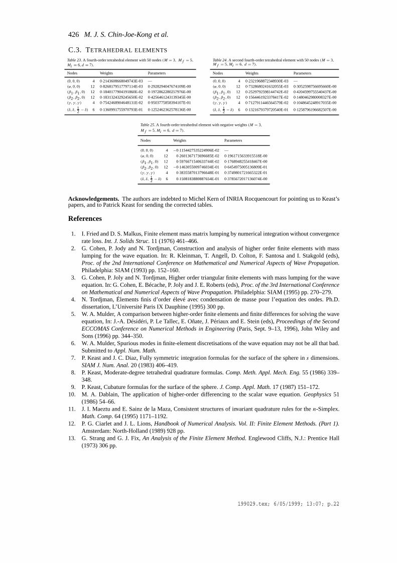
C.3. TETRAHEDRAL ELEMENTS

Table 23. A fourth-order tetrahedral element with 50 nodes(M = 3, Mf = 5,Mi = 6, d = 7).


(0,0,0) 4 0·2143608668049743E-03 —(α,0,0) 12 0·8268179517797114E-03 0·2928294047674109E-00(β1, β1,0) 12 0·1840177904191860E-02 0·1972862280257976E-00(β2, β2,0) 12 0·1831324329245650E-02 0·4256461243139345E-00(γ, γ, γ ) 4 0·7542468904648131E-02 0·9503775858394107E-01

(δ, δ, 12 − δ) 6 0·1360991755970793E-01 0·1252462362578136E-00

Table 24. A second fourth-order tetrahedral element with 50 nodes(M = 3,Mf = 5,Mi = 6, d = 7).


(0,0,0) 4 0·2321968872348930E-03 —(α,0,0) 12 0·7328680241632055E-03 0·3052598756695660E-00(β1, β1,0) 12 0·2529792598144742E-02 0·4204599755540437E-00(β2, β2,0) 12 0·1564461923378417E-02 0·1480462980008327E-00(γ, γ, γ ) 4 0·7127911446564579E-02 0·1048645248917035E-00

(δ, δ, 12 − δ) 6 0·1321679379720540E-01 0·1258796196682507E-00

Table 25. A fourth-order tetrahedral element with negative weights(M = 3,Mf = 5,Mi = 6, d = 7).


(0,0,0) 4 −0·1154427535224906E-02 —

(α,0,0) 12 0·2601367173696685E-02 0·1961715633915518E-00

(β1, β1,0) 12 0·5976671540633744E-02 0·1768948255418467E-00(β2, β2,0) 12 −0·1463055009746034E-01 0·6454975005136809E-01

(γ, γ, γ ) 4 0·3835587013796648E-01 0·3749801721665322E-01

(δ, δ, 12 − δ) 6 0·1508183880887654E-01 0·3785672017136074E-00

Acknowledgements.The authors are indebted to Michel Kern of INRIA Rocquencourt for pointing us to Keast’spapers, and to Patrick Keast for sending the corrected tables.

References

1. I. Fried and D. S. Malkus, Finite element mass matrix lumping by numerical integration without convergencerate loss.Int. J. Solids Struc.11 (1976) 461–466.

2. G. Cohen, P. Jody and N. Tordjman, Construction and analysis of higher order finite elements with masslumping for the wave equation. In: R. Kleinman, T. Angell, D. Colton, F. Santosa and I. Stakgold (eds),Proc. of the 2nd International Conference on Mathematical and Numerical Aspects of Wave Propagation.Philadelphia: SIAM (1993) pp. 152–160.

3. G. Cohen, P. Joly and N. Tordjman, Higher order triangular finite elements with mass lumping for the waveequation. In: G. Cohen, E. Bécache, P. Joly and J. E. Roberts (eds),Proc. of the 3rd International Conferenceon Mathematical and Numerical Aspects of Wave Propagation. Philadelphia: SIAM (1995) pp. 270–279.

4. N. Tordjman, Élements finis d’order élevé avec condensation de masse pour l’equation des ondes. Ph.D.dissertation, L’Université Paris IX Dauphine (1995) 300 pp.

5. W. A. Mulder, A comparison between higher-order finite elements and finite differences for solving the waveequation, In: J.-A. Désidéri, P. Le Tallec, E. Oñate, J. Périaux and E. Stein (eds),Proceedings of the SecondECCOMAS Conference on Numerical Methods in Engineering(Paris, Sept. 9–13, 1996), John Wiley andSons (1996) pp. 344–350.

6. W. A. Mulder, Spurious modes in finite-element discretisations of the wave equation may not be all that bad.Submitted toAppl. Num. Math.

7. P. Keast and J. C. Diaz, Fully symmetric integration formulas for the surface of the sphere ins dimensions.SIAM J. Num. Anal.20 (1983) 406–419.

8. P. Keast, Moderate-degree tetrahedral quadrature formulas.Comp. Meth. Appl. Mech. Eng.55 (1986) 339–348.

9. P. Keast, Cubature formulas for the surface of the sphere.J. Comp. Appl. Math.17 (1987) 151–172.10. M. A. Dablain, The application of higher-order differencing to the scalar wave equation.Geophysics51

(1986) 54–66.11. J. I. Maeztu and E. Sainz de la Maza, Consistent structures of invariant quadrature rules for then-Simplex.

Math. Comp. 64 (1995) 1171–1192.12. P. G. Ciarlet and J. L. Lions,Handbook of Numerical Analysis. Vol. II: Finite Element Methods. (Part 1).

Amsterdam: North-Holland (1989) 928 pp.13. G. Strang and G. J. Fix,An Analysis of the Finite Element Method. Englewood Cliffs, N.J.: Prentice Hall

(1973) 306 pp.

199029.tex; 6/05/1999; 13:07; p.22

Documents

Higher-order triangular and tetrahedral finite ... - CiteSeerX