Citation: Li, Yusheng, Shang, Yilun and Yang, Yiting (2017) Clustering coefficients of large networks. Information Sciences, 382. pp. 350-358. ISSN 0020-0255

Published by: Elsevier

URL: http://dx.doi.org/10.1016/j.ins.2016.12.027 <http://dx.doi.org/10.1016/j.ins.2016.12.027>

This version was downloaded from Northumbria Research Link: http://nrl.northumbria.ac.uk/36450/

Northumbria University has developed Northumbria Research Link (NRL) to enable users to access the University’s research output. Copyright ©  and moral rights for items on NRL are retained by the individual author(s) and/or other copyright owners. Single copies of full items can be reproduced, displayed or performed, and given to third parties in any format or medium for personal research or study, educational, or not-for-profit purposes without prior permission or charge, provided the authors, title and full bibliographic details are given, as well as a hyperlink and/or URL to the original metadata page. The content must not be changed in any way. Full items must not be sold commercially in any format or medium without formal permission of the copyright holder. The full policy is available online: http://nrl.northumbria.ac.uk/policies.html

This document may differ from the final, published version of the research and has been made available online in accordance with publisher policies. To read and/or cite from the published version of the research, please visit the publisher’s website (a subscription may be required.)

brought to you by COREView metadata, citation and similar papers at core.ac.uk

provided by Northumbria Research Link

Clustering coefficients of large networks∗

Yusheng Li, Yilun Shang†, Yiting YangDepartment of Mathematics, Tongji University

Shanghai 200092, China

Abstract

Let G be a network with n nodes and eigenvalues λ1 ≥ λ2 ≥ · · · ≥ λn. Then G iscalled an (n, d, λ)-network if it is d-regular and λ = max{|λ2|, |λ3|, . . . , |λn|}. It is shownthat if G is an (n, d, λ)-network and λ = O(

√d), the average clustering coefficient c(G) of G

satisfies c(G) ∼ d/n for large d. We show that this description also holds for strongly regulargraphs and Erdos-Renyi graphs. Although most real-world networks are not theoreticallyconstructed, we find that, interestingly, many of them have c(G) close to d/n, and manyclose to 1 − µ2(n−d−1)

d(d−1), where d is the average degree of G, and µ2 is the average of the

numbers of common neighbors over all non-adjacent pairs of nodes.

Key Words: Clustering coefficient; theoretic graph; real-world network

1 Introduction

Complex systems from various fields, such as physics, biology, and sociology, can be sys-tematically analyzed using their network representation. A network (also known as a graph)is composed of vertices (or nodes) and edges, where vertices represent the constitutes in thesystem and edges represent the relationships between these constitutes. Mathematically, wedefine G = (V,E) as a simple graph with vertex set V and edge set E ⊆ V × V . Denote byN(v) = {u ∈ V : uv ∈ E} the neighborhood of a vertex v, dv the degree of v, and ev = e(N(v))the number of edges in the subgraph of G induced by N(v), respectively.

An important measure of network topology, called clustering coefficient, assesses the triangu-lar pattern as well as the connectivity in a vertex’s neighborhood: a vertex has a high clusteringcoefficient if its neighbors tend to be directly connected with each other. The clustering coeffi-cient cv of a vertex v can be calculated as

cv =

{0, if dv = 0,ev

(dv2 ) , if dv ≥ 2.

∗Research supported by the National Natural Science Foundation of China under Grants No. 11331003,No. 11101360, No. 11505127, the Shanghai Pujiang Program under Grant No. 15PJ1408300, and OutstandingYoung Scholar Foundation of Tongji University under Grants No. 2013KJ031, No. 2014KJ036.

†Correspondence: shyl@tongji.edu.cn

1

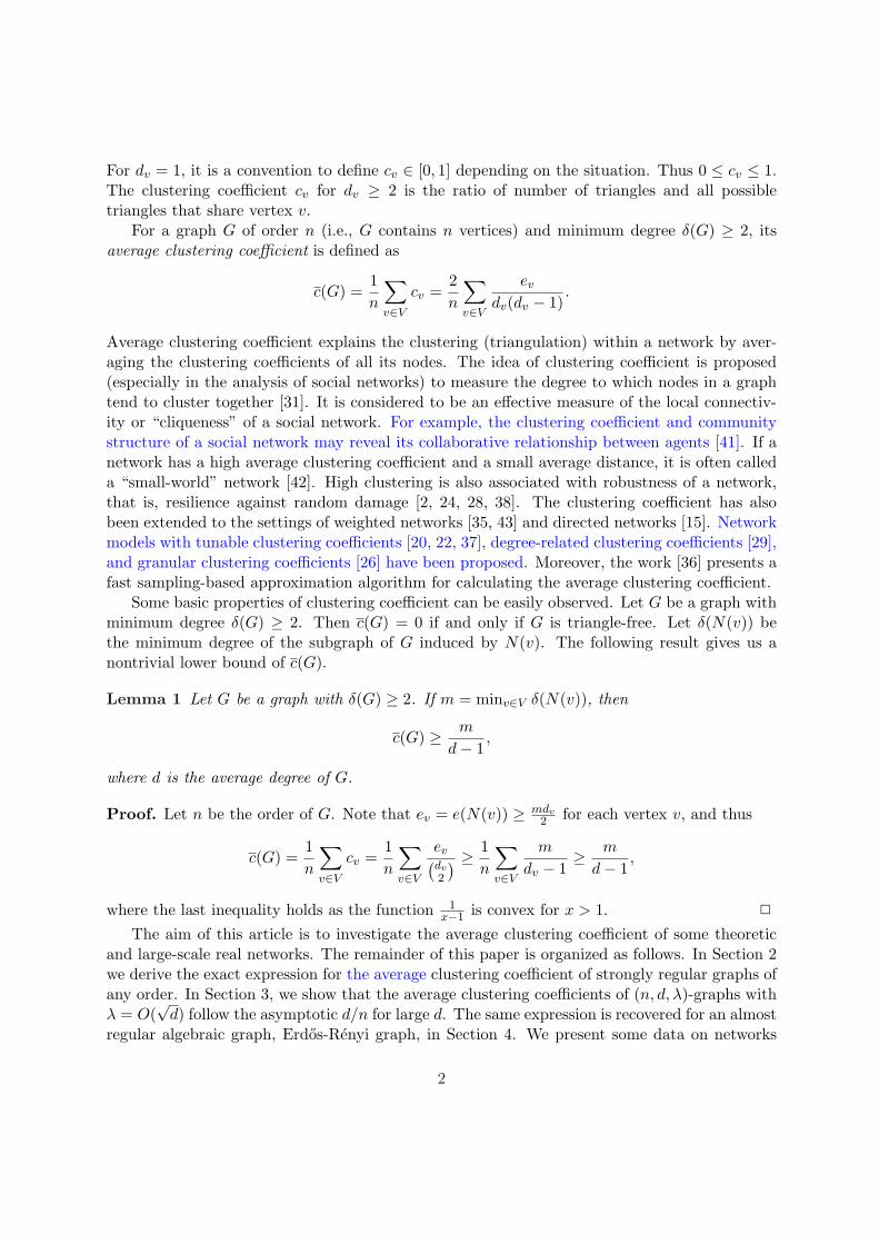
For dv = 1, it is a convention to define cv ∈ [0, 1] depending on the situation. Thus 0 ≤ cv ≤ 1.The clustering coefficient cv for dv ≥ 2 is the ratio of number of triangles and all possibletriangles that share vertex v.

For a graph G of order n (i.e., G contains n vertices) and minimum degree δ(G) ≥ 2, itsaverage clustering coefficient is defined as

c(G) =1n

∑v∈V

cv =2n

∑v∈V

ev

dv(dv − 1).

Average clustering coefficient explains the clustering (triangulation) within a network by aver-aging the clustering coefficients of all its nodes. The idea of clustering coefficient is proposed(especially in the analysis of social networks) to measure the degree to which nodes in a graphtend to cluster together [31]. It is considered to be an effective measure of the local connectiv-ity or “cliqueness” of a social network. For example, the clustering coefficient and communitystructure of a social network may reveal its collaborative relationship between agents [41]. If anetwork has a high average clustering coefficient and a small average distance, it is often calleda “small-world” network [42]. High clustering is also associated with robustness of a network,that is, resilience against random damage [2, 24, 28, 38]. The clustering coefficient has alsobeen extended to the settings of weighted networks [35, 43] and directed networks [15]. Networkmodels with tunable clustering coefficients [20, 22, 37], degree-related clustering coefficients [29],and granular clustering coefficients [26] have been proposed. Moreover, the work [36] presents afast sampling-based approximation algorithm for calculating the average clustering coefficient.

Some basic properties of clustering coefficient can be easily observed. Let G be a graph withminimum degree δ(G) ≥ 2. Then c(G) = 0 if and only if G is triangle-free. Let δ(N(v)) bethe minimum degree of the subgraph of G induced by N(v). The following result gives us anontrivial lower bound of c(G).

Lemma 1 Let G be a graph with δ(G) ≥ 2. If m = minv∈V δ(N(v)), then

c(G) ≥ m

d − 1,

where d is the average degree of G.

Proof. Let n be the order of G. Note that ev = e(N(v)) ≥ mdv2 for each vertex v, and thus

c(G) =1n

∑v∈V

cv =1n

∑v∈V

ev(dv

2

) ≥ 1n

∑v∈V

m

dv − 1≥ m

d − 1,

where the last inequality holds as the function 1x−1 is convex for x > 1. 2

The aim of this article is to investigate the average clustering coefficient of some theoreticand large-scale real networks. The remainder of this paper is organized as follows. In Section 2we derive the exact expression for the average clustering coefficient of strongly regular graphs ofany order. In Section 3, we show that the average clustering coefficients of (n, d, λ)-graphs withλ = O(

√d) follow the asymptotic d/n for large d. The same expression is recovered for an almost

regular algebraic graph, Erdos-Renyi graph, in Section 4. We present some data on networks

2

taken from real-world applications in Section 5. Interestingly, the average clustering coefficientof the Florentine families graph is shown to be close to the corresponding estimate obtainedfor strongly regular graphs (Theorem 1). Our finding highlights the fact that the asymptoticd/n is not only a characteristic of random graphs and some theoretic graphs, but also observedin various real systems distinct from small-world networks. Finally, the paper is concluded inSection 6.

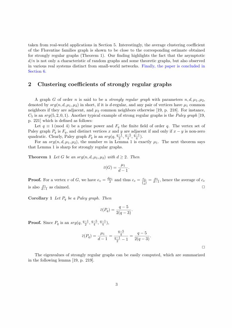
2 Clustering coefficients of strongly regular graphs

A graph G of order n is said to be a strongly regular graph with parameters n, d, µ1, µ2,denoted by srg(n, d, µ1, µ2) in short, if it is d-regular, and any pair of vertices have µ1 commonneighbors if they are adjacent, and µ2 common neighbors otherwise [19, p. 218]. For instance,C5 is an srg(5, 2, 0, 1). Another typical example of strong regular graphs is the Paley graph [19,p. 221] which is defined as follows:

Let q ≡ 1 (mod 4) be a prime power and Fq the finite field of order q. The vertex set ofPaley graph Pq is Fq, and distinct vertices x and y are adjacent if and only if x − y is non-zeroquadratic. Clearly, Paley graph Pq is an srg(q, q−1

2 , q−54 , q−1

4 ).For an srg(n, d, µ1, µ2), the number m in Lemma 1 is exactly µ1. The next theorem says

that Lemma 1 is sharp for strongly regular graphs.

Theorem 1 Let G be an srg(n, d, µ1, µ2) with d ≥ 2. Then

c(G) =µ1

d − 1.

Proof. For a vertex v of G, we have ev = dµ1

2 and thus cv = ev

(d2)

= µ1

d−1 , hence the average of cv

is also µ1

d−1 as claimed. 2

Corollary 1 Let Pq be a Paley graph. Then

c(Pq) =q − 5

2(q − 3).

Proof. Since Pq is an srg(q, q−12 , q−5

4 , q−14 ),

c(Pq) =µ1

d − 1=

q−54

q−12 − 1

=q − 5

2(q − 3).

2

The eigenvalues of strongly regular graphs can be easily computed, which are summarizedin the following lemma [19, p. 219].

3

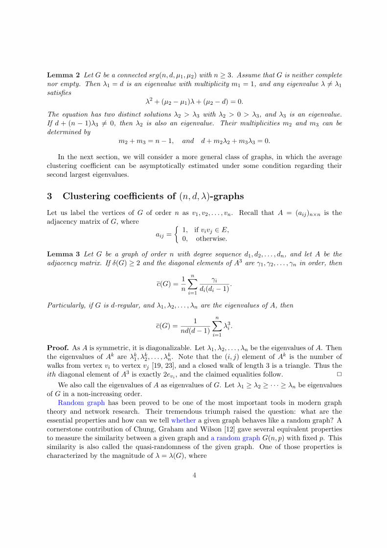
Lemma 2 Let G be a connected srg(n, d, µ1, µ2) with n ≥ 3. Assume that G is neither completenor empty. Then λ1 = d is an eigenvalue with multiplicity m1 = 1, and any eigenvalue λ 6= λ1

satisfiesλ2 + (µ2 − µ1)λ + (µ2 − d) = 0.

The equation has two distinct solutions λ2 > λ3 with λ2 > 0 > λ3, and λ3 is an eigenvalue.If d + (n − 1)λ3 6= 0, then λ2 is also an eigenvalue. Their multiplicities m2 and m3 can bedetermined by

m2 + m3 = n − 1, and d + m2λ2 + m3λ3 = 0.

In the next section, we will consider a more general class of graphs, in which the averageclustering coefficient can be asymptotically estimated under some condition regarding theirsecond largest eigenvalues.

3 Clustering coefficients of (n, d, λ)-graphs

Let us label the vertices of G of order n as v1, v2, . . . , vn. Recall that A = (aij)n×n is theadjacency matrix of G, where

aij ={

1, if vivj ∈ E,0, otherwise.

Lemma 3 Let G be a graph of order n with degree sequence d1, d2, . . . , dn, and let A be theadjacency matrix. If δ(G) ≥ 2 and the diagonal elements of A3 are γ1, γ2, . . . , γn in order, then

c(G) =1n

n∑i=1

γi

di(di − 1).

Particularly, if G is d-regular, and λ1, λ2, . . . , λn are the eigenvalues of A, then

c(G) =1

nd(d − 1)

n∑i=1

λ3i .

Proof. As A is symmetric, it is diagonalizable. Let λ1, λ2, . . . , λn be the eigenvalues of A. Thenthe eigenvalues of Ak are λk

1, λk2, . . . , λ

kn. Note that the (i, j) element of Ak is the number of

walks from vertex vi to vertex vj [19, 23], and a closed walk of length 3 is a triangle. Thus theith diagonal element of A3 is exactly 2evi , and the claimed equalities follow. 2

We also call the eigenvalues of A as eigenvalues of G. Let λ1 ≥ λ2 ≥ · · · ≥ λn be eigenvaluesof G in a non-increasing order.

Random graph has been proved to be one of the most important tools in modern graphtheory and network research. Their tremendous triumph raised the question: what are theessential properties and how can we tell whether a given graph behaves like a random graph? Acornerstone contribution of Chung, Graham and Wilson [12] gave several equivalent propertiesto measure the similarity between a given graph and a random graph G(n, p) with fixed p. Thissimilarity is also called the quasi-randomness of the given graph. One of those properties ischaracterized by the magnitude of λ = λ(G), where

4

λ = λ(G) = max{|λi| : 2 ≤ i ≤ n}.

As called by Alon, see [4], a graph G is an (n, d, λ)-graph if G is d-regular with n vertices andλ = λ(G). Note that a d-regular connected graph satisfies that λ1 = d. For sparse graphswith edge density p = o(1), Chung and Graham [11] also gave some equivalent properties forquasi-randomness under certain conditions. One of the properties is that λ1 ∼ pn and λ = o(λ1).

For an (n, d, λ)-graph, the spectral gap between d and λ is a measure for its quasi-randomproperty. The smaller the value of λ compared to d, the closer is the edge distribution to theideal uniform distribution (i.e., it becomes a random graph). A natural question in order is“how small can λ be?”

Lemma 4 Let G be an (n, d, λ)-graph and let ε > 0. If d ≤ (1 − ε)n, then

λ ≥√

εd.

Proof. Let A be the adjacency matrix of G. Then

nd = 2e(G) = tr(A2) =n∑

i=1

λ2i

≤ d2 + (n − 1)λ2 ≤ (1 − ε)nd + nλ2,

which concludes the proof. 2

Based on this estimate, we may say, not precisely, that an (n, d, λ)-graph with λ = O(√

d)has good quasi-randomness. Generally, this is a weak condition as most random graphs are suchgraphs, see [7]. Moreover, Lemma 2 suggests that for an srg(n, d, µ1, µ2), when |µ1−µ2| is smallcompared to d, λ is close to

√d and G has good quasi-randomness.

It is known that, for any fixed d ≥ 4, a random d-regular graph G of order n has λ =(2 + o(1))

√d − 1 and for any fixed ε > 0, the probability

Pr((1 − ε)

d − 1n

≤ c(G) ≤ (1 + ε)d − 1

n

)→ 1

as n → ∞ [8, 17]. The following theorem gives an analogous estimate of average clusteringcoefficient for (n, d, λ)-graph with λ = O(

√d).

Theorem 2 Let G be an (n, d, λ)-graph. If λ = O(√

d) as d → ∞, then

c(G) ∼ d

n.

Proof. Let n be the order of G whose eigenvalues are λ1 ≥ λ2 ≥ · · · ≥ λn. Since G is d-regular,we have λ1 = d. From Lemma 3 we obtain

c(G) =1

nd(d − 1)

(d3 +

n∑i=2

λ3i

).

5

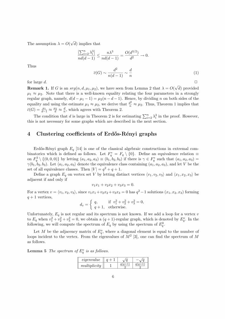
The assumption λ = O(√

d) implies that∣∣∑ni=2 λ3

i

∣∣nd(d − 1)

≤ nλ3

nd(d − 1)=

O(d3/2)d2

→ 0.

Thus

c(G) ∼ d2

n(d − 1)∼ d

n(1)

for large d. 2

Remark 1. If G is an srg(n, d, µ1, µ2), we have seen from Lemma 2 that λ = O(√

d) providedµ1 ≈ µ2. Note that there is a well-known equality relating the four parameters in a stronglyregular graph, namely, d(d− µ1 − 1) = µ2(n− d− 1). Hence, by dividing n on both sides of theequality and using the estimate µ1 ≈ µ2, we derive that d2

n ≈ µ2. Thus, Theorem 1 implies thatc(G) = µ1

d−1 ≈ µ2

d ≈ dn , which agrees with Theorem 2.

The condition that d is large in Theorem 2 is for estimating∑n

i=2 λ3i in the proof. However,

this is not necessary for some graphs which are described in the next section.

4 Clustering coefficients of Erdos-Renyi graphs

Erdos-Renyi graph Eq [14] is one of the classical algebraic constructions in extremal com-binatorics which is defined as follows. Let F ∗

q = Fq \ {0}. Define an equivalence relation ≡on F 3

q \ {(0, 0, 0)} by letting (a1, a2, a3) ≡ (b1, b2, b3) if there is γ ∈ F ∗q such that (a1, a2, a3) =

γ(b1, b2, b3). Let 〈a1, a2, a3〉 denote the equivalence class containing (a1, a2, a3), and let V be theset of all equivalence classes. Then |V | = q2 + q + 1.

Define a graph Eq on vertex set V by letting distinct vertices 〈v1, v2, v3〉 and 〈x1, x2, x3〉 beadjacent if and only if

v1x1 + v2x2 + v3x3 = 0.

For a vertex v = 〈v1, v2, v3〉, since v1x1 +v2x2 +v3x3 = 0 has q2−1 solutions (x1, x2, x3) formingq + 1 vertices,

dv ={

q, if v21 + v2

2 + v23 = 0,

q + 1, otherwise.

Unfortunately, Eq is not regular and its spectrum is not known. If we add a loop for a vertex vto Eq when v2

1 + v22 + v2

3 = 0, we obtain a (q + 1)-regular graph, which is denoted by Eoq . In the

following, we will compute the spectrum of Eq by using the spectrum of E0q .

Let M be the adjacency matrix of Eoq , where a diagonal element is equal to the number of

loops incident to the vertex. From the eigenvalues of M2 [3], one can find the spectrum of Mas follows.

Lemma 5 The spectrum of Eoq is as follows.

eigenvalue q + 1√

q −√q

multiplicity 1 q(q+1)2

q(q+1)2

6

Return to the simple graph Eq with maximum degree ∆(Eq) = q + 1 and minimum degreeδ(Eq) = q. Let A be the adjacency matrix of Eq and λ1 ≥ λ2 ≥ · · · ≥ λn the eigenvalues of A,where n = q2 + q + 1. We shall estimate these {λi}n

i=1 by the following result, see [23, p. 181].

Lemma 6 Let A and B be real symmetric matrices of order n. Let the eigenvalues λi(A) of A,λi(B) of B and λi(A + B) of A + B are labeled in non-increasing order, respectively. Then, foreach 1 ≤ i ≤ n,

λi(A) + λ1(B) ≥ λi(A + B) ≥ λi(A) + λn(B).

Corollary 2 Let G be a simple graph of order n with ∆ = ∆(G) and δ = δ(G). Let G′ be agraph obtained from G by attaching each vertex v with ∆−dv loops. Suppose that G and G′ haveeigenvalues λ1 ≥ λ2 ≥ · · · ≥ λn and λ′

1 ≥ λ′2 ≥ · · · ≥ λ′

n, respectively. Then, for each 1 ≤ i ≤ n,

λi + ∆ − δ ≥ λ′i ≥ λi.

Proof. It is easy to see that A(G′) = A(G) + D, where D is a diagonal matrix whose diagonalelements are ∆−dv for each vertex v. Since λ1(D) = ∆−δ and λn(D) = 0, the assertion followsfrom Lemma 6. 2

Lemma 7 Let λ1 ≥ λ2 ≥ · · · ≥ λn be eigenvalues of Eq, where n = q2 + q + 1. Then theseeigenvalues can be bounded as follows.

eigenvalue λ1 λi; λi > 0, i ≥ 2 λi; λi < 0bounds q ≤ λ1 ≤ q + 1

√q ≤ λi ≤

√q + 1 −√

q ≤ λi ≤ −√q + 1

Although Eq is not regular, c(Eq) is still close to d/n, where n = q2 + q + 1 and d is theaverage degree of Eq.

Theorem 3 Let q be a prime power and let Eq be the Erdos-Renyi graph. Then Eq has n =q2 + q + 1 vertices and its average degree d satisfies q < d < q + 1, and c(Eq) ∼ d

n ∼ 1q for large

q.

Proof. It is easy to see that except the largest λ1, the number of other positive eigenvalues isq(q + 1)/2 and the number of negative eigenvalues is also q(q + 1)/2. So we can estimate

∑i λ

3i

from above as∑i

λ3i ≤ (q + 1)3 +

q(q + 1)2

(√

q + 1) − q(q + 1)2

(√

q − 1) = (q + 1)3 + q(q + 1),

and thus by Lemma 3 we have

c(Eq) ≤(q + 1)3 + q(q + 1)(q2 + q + 1)q(q − 1)

∼ 1q,

and the desired lower bound can be obtained similarly. 2

7

5 Clustering coefficients of some real networks

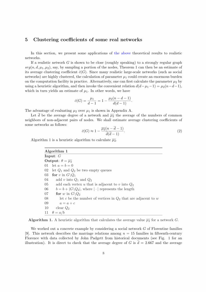
In this section, we present some applications of the above theoretical results to realisticnetworks.

If a realistic network G is shown to be close (roughly speaking) to a strongly regular graphsrg(n, d, µ1, µ2), say, by sampling a portion of the nodes, Theorem 1 can then be an estimate ofits average clustering coefficient c(G). Since many realistic large-scale networks (such as socialnetworks) are highly clustered, the calculation of parameter µ1 could create an enormous burdenon the computation facility in practice. Alternatively, one can first calculate the parameter µ2 byusing a heuristic algorithm, and then invoke the convenient relation d(d−µ1−1) = µ2(n−d−1),which in turn yields an estimate of µ1. In other words, we have

c(G) =µ1

d − 1= 1 − µ2(n − d − 1)

d(d − 1).

The advantage of evaluating µ2 over µ1 is shown in Appendix A.Let d be the average degree of a network and µ2 the average of the numbers of common

neighbors of non-adjacent pairs of nodes. We shall estimate average clustering coefficients ofsome networks as follows:

c(G) ≈ 1 − µ2(n − d − 1)d(d − 1)

. (2)

Algorithm 1 is a heuristic algorithm to calculate µ2.

Algorithm 1Input: GOutput: θ = µ2

01 let a = b = 002 let Q1 and Q2 be two empty queues03 for v in G\Q1

04 add v into Q1 and Q2

05 add each vertex u that is adjacent to v into Q2

06 b = b + |G\Q2|, where | · | represents the length07 for w in G\Q2

08 let c be the number of vertices in Q2 that are adjacent to w09 a = a + c10 clear Q2

11 θ = a/b

Algorithm 1. A heuristic algorithm that calculates the average value µ2 for a network G.

We worked out a concrete example by considering a social network G of Florentine families[9]. This network describes the marriage relations among n = 15 families in fifteenth-centuryFlorence with data collected by John Padgett from historical documents (see Fig. 1 for anillustration). It is direct to check that the average degree of G is d = 2.667 and the average

8

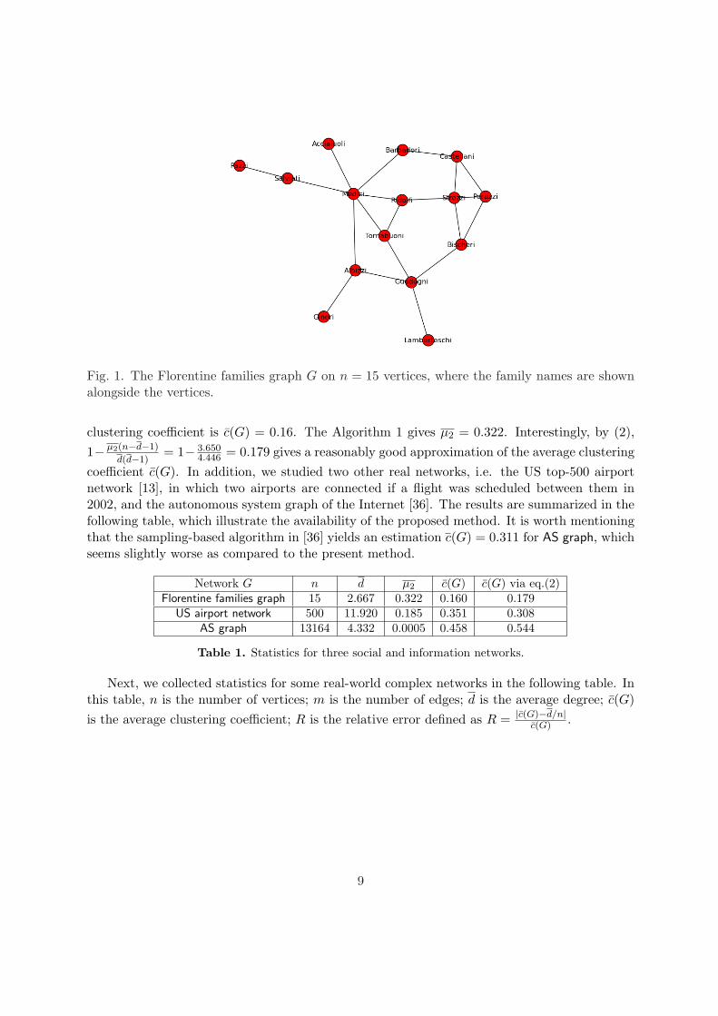
Fig. 1. The Florentine families graph G on n = 15 vertices, where the family names are shownalongside the vertices.

clustering coefficient is c(G) = 0.16. The Algorithm 1 gives µ2 = 0.322. Interestingly, by (2),1− µ2(n−d−1)

d(d−1)= 1− 3.650

4.446 = 0.179 gives a reasonably good approximation of the average clusteringcoefficient c(G). In addition, we studied two other real networks, i.e. the US top-500 airportnetwork [13], in which two airports are connected if a flight was scheduled between them in2002, and the autonomous system graph of the Internet [36]. The results are summarized in thefollowing table, which illustrate the availability of the proposed method. It is worth mentioningthat the sampling-based algorithm in [36] yields an estimation c(G) = 0.311 for AS graph, whichseems slightly worse as compared to the present method.

Network G n d µ2 c(G) c(G) via eq.(2)Florentine families graph 15 2.667 0.322 0.160 0.179

US airport network 500 11.920 0.185 0.351 0.308AS graph 13164 4.332 0.0005 0.458 0.544

Table 1. Statistics for three social and information networks.

Next, we collected statistics for some real-world complex networks in the following table. Inthis table, n is the number of vertices; m is the number of edges; d is the average degree; c(G)is the average clustering coefficient; R is the relative error defined as R = |c(G)−d/n|

c(G) .

9

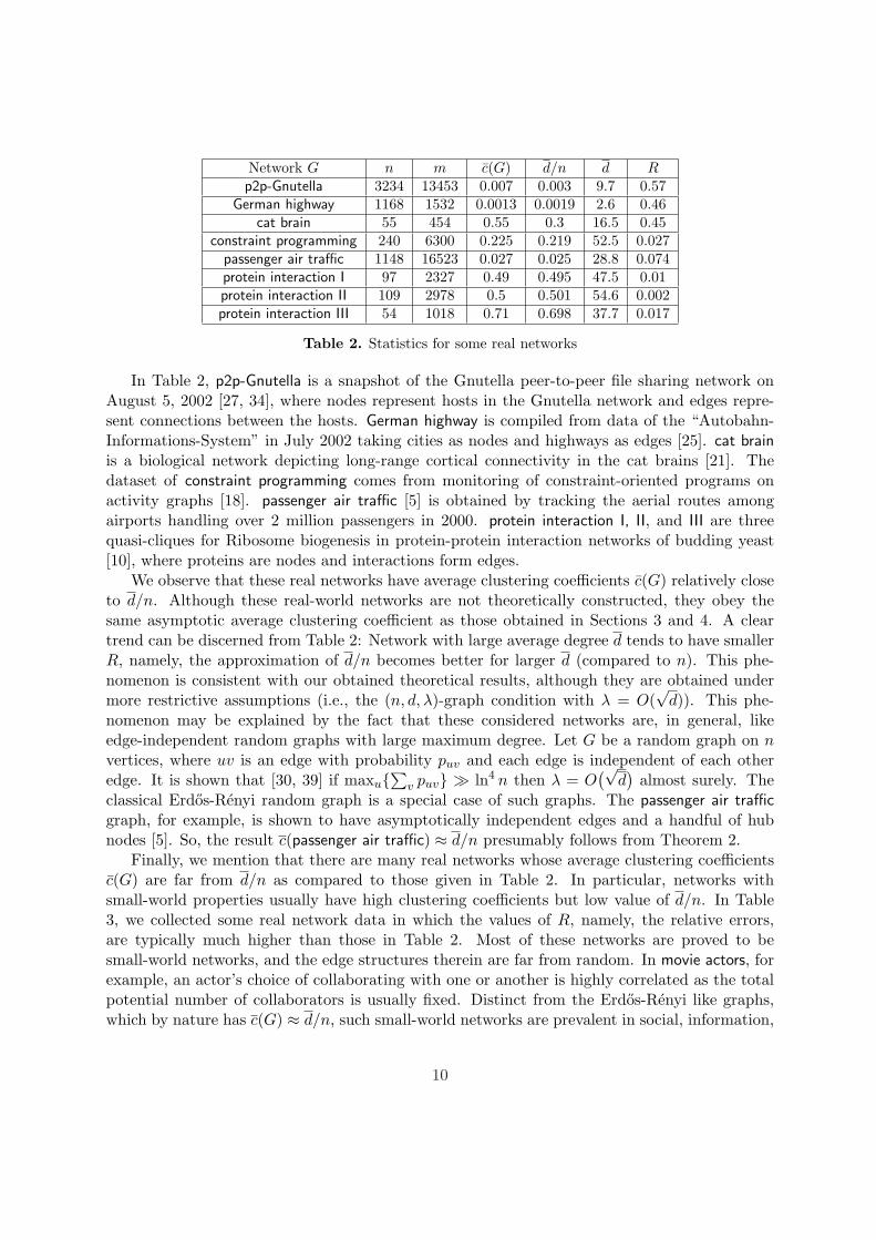
Network G n m c(G) d/n d Rp2p-Gnutella 3234 13453 0.007 0.003 9.7 0.57

German highway 1168 1532 0.0013 0.0019 2.6 0.46cat brain 55 454 0.55 0.3 16.5 0.45

constraint programming 240 6300 0.225 0.219 52.5 0.027passenger air traffic 1148 16523 0.027 0.025 28.8 0.074protein interaction I 97 2327 0.49 0.495 47.5 0.01protein interaction II 109 2978 0.5 0.501 54.6 0.002protein interaction III 54 1018 0.71 0.698 37.7 0.017

Table 2. Statistics for some real networks

In Table 2, p2p-Gnutella is a snapshot of the Gnutella peer-to-peer file sharing network onAugust 5, 2002 [27, 34], where nodes represent hosts in the Gnutella network and edges repre-sent connections between the hosts. German highway is compiled from data of the “Autobahn-Informations-System” in July 2002 taking cities as nodes and highways as edges [25]. cat brainis a biological network depicting long-range cortical connectivity in the cat brains [21]. Thedataset of constraint programming comes from monitoring of constraint-oriented programs onactivity graphs [18]. passenger air traffic [5] is obtained by tracking the aerial routes amongairports handling over 2 million passengers in 2000. protein interaction I, II, and III are threequasi-cliques for Ribosome biogenesis in protein-protein interaction networks of budding yeast[10], where proteins are nodes and interactions form edges.

We observe that these real networks have average clustering coefficients c(G) relatively closeto d/n. Although these real-world networks are not theoretically constructed, they obey thesame asymptotic average clustering coefficient as those obtained in Sections 3 and 4. A cleartrend can be discerned from Table 2: Network with large average degree d tends to have smallerR, namely, the approximation of d/n becomes better for larger d (compared to n). This phe-nomenon is consistent with our obtained theoretical results, although they are obtained undermore restrictive assumptions (i.e., the (n, d, λ)-graph condition with λ = O(

√d)). This phe-

nomenon may be explained by the fact that these considered networks are, in general, likeedge-independent random graphs with large maximum degree. Let G be a random graph on nvertices, where uv is an edge with probability puv and each edge is independent of each otheredge. It is shown that [30, 39] if maxu{

∑v puv} À ln4 n then λ = O

(√d)

almost surely. Theclassical Erdos-Renyi random graph is a special case of such graphs. The passenger air trafficgraph, for example, is shown to have asymptotically independent edges and a handful of hubnodes [5]. So, the result c(passenger air traffic) ≈ d/n presumably follows from Theorem 2.

Finally, we mention that there are many real networks whose average clustering coefficientsc(G) are far from d/n as compared to those given in Table 2. In particular, networks withsmall-world properties usually have high clustering coefficients but low value of d/n. In Table3, we collected some real network data in which the values of R, namely, the relative errors,are typically much higher than those in Table 2. Most of these networks are proved to besmall-world networks, and the edge structures therein are far from random. In movie actors, forexample, an actor’s choice of collaborating with one or another is highly correlated as the totalpotential number of collaborators is usually fixed. Distinct from the Erdos-Renyi like graphs,which by nature has c(G) ≈ d/n, such small-world networks are prevalent in social, information,

10

and biological systems. Much effort on the study of clustering coefficients has been devoted tosuch networks with small-world phenomenon [31].

Network G n m c(G) d/n d RWWW [1] 153127 2695801 0.1078 0.00023 35.21 0.998

movie actors [42] 225226 6869393 0.79 0.00027 61 0.999SPIRES co-authorship [32] 56627 4898236 0.726 0.003 173 0.996Neurosci. co-authorship [6] 209293 1203435 0.76 0.000005 11.5 0.999

E. coli substrate [16] 282 1036 0.32 0.026 7.35 0.919E. coli reaction [16] 315 4475 0.59 0.09 28.3 0.847

C. Elegans [42] 282 1974 0.28 0.05 14 0.821

Table 3. Statistics for some real small-world networks, where the value R is typically very high.

6 Conclusion

In this paper, we have shown analytically that the average clustering coefficient c(G) of an(n, d, λ)-network G with λ = O(

√d) satisfies c(G) ∼ d/n for large d. This asymptotic expression

also holds for strongly regular graphs and Erdos-Renyi graphs. In addition to the above theoreticgraphs, we present numerical results based on real network data.

Our key finding, that a range of networks possess the asymptotic average clustering coefficientd/n, where d is the empirical average degree of the network in question, as opposed to the small-world networks, suggests a new category of Erdos-Renyi like networks, which we hope couldshed some lights on the network clustering phenomenon and stimulate further research effortson the related topics.

Appendix A

For a graph G = (V,E), let M1 =∑

uv∈E |{w ∈ V : w ∈ N(u) ∩ N(v)}| be the total number ofcommon neighbors of adjacent vertices. Similarly, let M2 =

∑uv 6∈E |{w ∈ V : w ∈ N(u)∩N(v)}|

be the total number of common neighbors of non-adjacent vertices. Apparently, the complexityof computing µi is proportional to Mi (i = 1, 2). In Fig. 2 we show an illustrating examplefor a moderately clustered network, where M1 = 2M2, meaning that using (2) could halve thecomputational burden.

We show in Fig. 3 the ratio M2/M1 for general random networks created by the clusteredrandom graph model following [33]. This model is basically the configuration random graphdecorated by two sequences, i.e., ti, the number of triangles in which the i-th vertex participates,and si, the number of single edges attached to the i-th vertex, other than those belonging to thetriangles. We observe from Fig. 3 that 0 < M2/M1 < 0.8 for networks of all orders considered,suggesting that our use of (2) could effectively reduce the computational burden for clusterednetworks.

11

Fig. 2. Left: a network with 5 vertices. Right: the associated table consisting of the numbersof common neighbors of each pair of vertices, where blue numbers indicate adjacent pairs ofvertices while red numbers indicate non-adjacent pairs. Hence, M1 = 12 and M2 = 6.

0 100 200 300 400 5000

0.2

0.4

0.6

0.8

1

M2/M

1

n

Fig. 3. The ratio M2/M1 versus n, the number of vertices, for clustered random graphs withti, si ∈ {1, 2, · · · , 5} uniformly at random. Each data point is based upon averaging over asample of 30 independent realizations.

Acknowledgement

The authors are very thankful to the editor and anonymous reviewers for their valuable commentsand constructive suggestions that greatly help them improve the presentation of the manuscript.

References

[1] L. A. Adamic and B. A. Huberman, Growth dynamics of the World Wide Web, Nature,401 (1999), 131.

[2] S. Agreste, S. Catanese, P. D. Meo, E. Ferrara, G. Fiumara, Network structure and resilienceof Mafia syndicates, Inf. Sci., 351 (2016), 30-47.

[3] M. Aigner and G. Ziegler, Proofs from THE BOOK (3rd ed.), Springer, 2004.

12

[4] N. Alon and J. Spencer, The Probabilistic Method, 3rd ed., Wiley-Interscience, New York,2008.

[5] M. Amiel, G. Melancon, and C. Rozenblat. Reseaux multi-niveaux : l’exemple des echangesaeriens mondiaux de passagers. M@ppemonde, 79 (2005), 05302.

[6] A.-L. Barabasi, H. Jeonga, Z. Neda, E. Ravasz, A. Schubert, and T. Vicsek, Evolution ofthe social network of scientific collaborations, Physica A, 311 (2002), 590-614.

[7] B. Bollobas, Random Graphs (2nd ed.), Cambridge University Press, London-New York,2001.

[8] B. Bollobas and O. Riordan, Mathematical results on scale-free random graphs, in Handbookof Graphs and Networks: From the Genome to the Internet (eds. S. Bornholdt and H. G.Schuster), pp. 1-34, Wiley-VCH, Berlin, 2002.

[9] R. L. Breiger and P. E. Pattison, Cumulated social roles: the duality of persons and theiralgebras, Social Networks, 8 (1986), 215-256.

[10] D. Bu, Y. Zhao, L. Cai, H. Xue, X. Zhu, H. Lu, J. Zhang, S. Sun, L. Ling, N. Zhang, G.Li, and R. Chen, Topological structure analysis of the protein-protein interaction networkin budding yeast, Nucleic Acids Research, 31 (2003), 2443-2450.

[11] F. R. Chung and R. Graham, Sparse quasi-random graphs, Combinatoria, 22 (2002), 217-244.

[12] F. R. Chung, R. Graham, and R. Wilson, Quasi-random graphs, Combinatoria, 9 (1989),345-362.

[13] V. Colizza, R. Pastor-Satorras, and A. Vespignani, Reaction-diffusion processes andmetapopulation models in heterogeneous networks, Nature Physics, 3 (2007), 276-282.

[14] P. Erdos, and A. Reyi, On a problem in theory of graphs, Publ. Math. Inst. Hungar. acad.Sci., 7A (1962), 623-641.

[15] G. Fagiolo, Clustering in complex directed networks, Phys. Rev. E, 76 (2007), 026107.

[16] D. A. Fell and A. Wagner, The small world of metabolism, Nat. Biotechnol, 18 (2000),1121-1122.

[17] J. Friedman, A proof of Alon’s second eigenvalue conjecture and related problems, Mem.Amer. Math. Soc., 195 (2008), #910.

[18] M. Ghoniem, Outils de visualisation et d’aide a la mise au point de programmes aveccontraintes. Phd, Universite de Nantes, 2005.

[19] C. Godsil and G. Royle, Algebraic Graph Theory, Springer, 2001.

[20] L. S. Heath, N. Parikh, Generating random graphs with tunable clustering coefficients,Physica A, 390 (2011), 4577-4587.

13

[21] C. Hilgetag, G. A. P. C. Burns, M. A. O’Neill, J. W. Scannell, and M. P. Young, Anatomicalconnectivity defines the organization of clusters of cortical areas in the macaque monkeyand the cat, Philos. Trans. R. Soc. London, Ser. B, 355 (2000), 91-110.

[22] P. Holme and B. J. Kim, Growing scale-free networks with tunable clustering, Phys. Rev.E, 65 (2002), 026107.

[23] R. Horn and C. Johnson, Matrix Analysis, Cambridge University Press, London, 1986.

[24] S. Iyer, T. Killingback, B. Sundaram, and Z. Wang, Attack robustness and centrality ofcomplex networks, PLoS One, 8 (2013), e59613.

[25] M. Kaiser and C. C. Hilgetag, Spatial growth of real-world networks, Phys. Rev. E, 69(2004), 036103.

[26] S. Kundu, S. K. Pal, FGSN: fuzzy granular social networks - model and applications, Inf.Sci., 314 (2015), 100-117.

[27] J. Leskovec, J. Kleinberg, and C. Faloutsos, Graph evolution: densification and shrinkingdiameters, ACM Transactions on Knowledge Discovery from Data, 1 (2007), 2.

[28] M. Li and C. O’Riordan, The effect of clustering coefficient and node degree on the robust-ness of cooperation, 2013 IEEE Congress on Evolutionary Computation, Cancun, 2013,2833-2839.

[29] Y. Liu, C. Zhao, X. Wang, Q. Huang, X. Zhang, D. Yi, The degree-related clusteringcoefficient and its application to link prediction, Physica A, 454 (2016), 24-33.

[30] L. Lu and X. Peng, Spectra of edge-independent random graphs, Electron. J. Combin., 20(2013), #P27.

[31] M. E. J. Newman, Networks: An Introduction, Oxford University Press, New York, 2010.

[32] M. E. J. Newman, Scientific collaboration networks. I. Network construction and funda-mental results, Phys. Rev. E, 64 (2001), 016131.

[33] M. E. J. Newman, Random graphs with clustering, Phys. Rev. E, 103 (2009), 058701.

[34] M. Ripeanu, I. Foster, and A. Iamnitchi, Mapping the Gnutella network: properties of large-scale peer-to-peer systems and implications for system design, IEEE Internet ComputingJournal, 6 (2002), 50-57.

[35] J. Saramaki, M. Kivela, J.-P. Onnela, K. Kaski, and J. Kertesz, Generalizations of theclustering coefficient to weighted complex networks, Phys. Rev. E, 75 (2007), 027105.

[36] T. Schank and D. Wagner, Approximating clustering coefficient and transitivity, J. GraphAlgor. Appl., 9 (2005), 265-275.

[37] Y. Shang, Distinct clusterings and characteristic path lengths in dynamic small-world net-works with identical limit degree distribution, J. Stat. Phys., 149 (2012), 505-518.

14

[38] Y. Shang, Unveiling robustness and heterogeneity through percolation triggered by random-link breakdown, Phys. Rev. E, 90 (2014) 032820.

[39] Y. Shang, Bounding extremal degrees of edge-independent random graphs using relativeentropy, Entropy, 18 (2016), #53.

[40] T. Szabo, On the spectrum of projective norm-graphs, Inform. Process. Lett., 86 (2003),71-74.

[41] S. Wang, L. Huang, C.-H. Hsu, F. Yang, Collaboration reputation for trustworthy Webservice selection in social networks, J. Comput. Syst. Sci., 82 (2016), 130-143.

[42] D. J. Watts and S. Strogatz, Collective dynamics of “small-world” networks, Nature, 393(1998), 440-442.

[43] B. Zhang and S. Horvath, A general framework for weighted gene co-expression networkanalysis, Stat. Appl. Genet. Mol. Biol., 4 (2005), 17.

15