Circularity error evaluation

Circularity error evaluationtheory and algorithm

M. Wang, S. Hossein Cheraghi*, Abu S.M. MasudDepartment of Industrial and Manufacturing Engineering, Wichita State University, Wichita, KS, 67260-0035, USA

Received 5 October 1998; accepted 13 January 1999

Abstract

Many procedures for the evaluation of circularity error based on different criteria have been developed. The procedures that are basedon the minimum radial separation criterion are either too complex or lack an algorithmic approach to find optimal solution. This paperpresents an optimization-based technique to find the value of circularity error based on the minimum radial separation criterion. The problemis formulated as a nonlinear optimization problem. Based on the developed necessary and sufficient conditions a generalized nonlinearoptimization procedure is presented. The performance of the developed procedure is analyzed for different size problems generated usinga simulation program. Results indicate that the procedure is accurate and very efficient in solving large size real life problems. © 1999Elsevier Science Inc. All rights reserved.

Keywords:Circularity; Minimum radial separation; Optimization

1. Introduction

Accurate measurement of the circularity error is verycritical because most mechanical parts comprise circularelements (internal and external). For a feature other than asphere, as defined by the ASME Y14.5M-1994 standards onGeometric Dimensioning and Tolerancing (GD&T), circu-larity is a condition of a surface where all points of thesurface intersected by any plane perpendicular to an axis areequidistant from that axis. Circularity tolerance specifies atolerance zone bounded by two concentric circles withinwhich each circular element of the surface must lie [1].

Measurement techniques for circularity error can be di-vided into two general methods: theintrinsic datummethodand the extrinsic datummethod. In the intrinsic datummethod, points on the surface of the part are used as adatum. The most commonly used intrinsic techniques arediametrical measurements, V-block measurements, andbench center measurements. With diametrical measurementtechnique, a simple measurement device, such as a micro-meter, an air gauge, or a bore gauge, is used, and thediameter of a part is measured at several cross sections.

With the V-block technique, the part is rotated inside aV-block, and a dial indicator is used to check the circularityerror. With the bench center technique, the part is rotatedbetween two accurate centers, and the error is measuredusing a dial indicator.

In the extrinsic method, an external member is used asthe datum reference. There are four common measuringtechniques under this category: least-square circle (LSC),maximum inscribed circle (MIC), minimum circumscribedcircle (MCC), and minimum radial separation (MRS) circle.With the LSC method, a circle is fitted to the profile usingthe least-square method. The center of that circle is used tofit the smallest circumscribed and the largest inscribed cir-cles to the profile. The radial difference between these twocircles is used as a measure of circularity error. With theMIC method, the center of the largest circle that can becontained inside the profile without including any part of theprofile is found. That center is then used to find the smallestcircle that contains the profile. The radial distance betweenthe two circles provides the circularity error. With the MCCmethod, the smallest circle that contains the profile is firstfound. The center of that circle is then used to find thelargest inscribed circle. The radial difference between thesetwo circles is the circularity error. With the MRS method,two concentric circles with minimum radial separation arefound that contain the profile. The radial difference between

* Corresponding author. Tel.:1316-978-3425; fax:1316-978-3742.E-mail address:[email protected] (H. Cheraghi)

Precision Engineering 23 (1999) 164–176

0141-6359/99/$ – see front matter © 1999 Elsevier Science Inc. All rights reserved.PII: S0141-6359(99)00006-9

these two circles provides the value for the circularity error.Of the techniques mentioned above, only the MRS methodcomplies with the ASME Y14.5-1994 standards on GD&T.

Mathematical procedures exist that can efficiently findthe LSC, MIC, and MCC for calculating the circularityerror. The techniques based on the MRS method are eithercomplex or lack an algorithmic approach to find the optimalsolution. This paper presents the underlying theory and analgorithm for the evaluation of circularity error based on theMRS criterion. An infinitesimal analysis method is used toanalyze the characteristics of the circularity function in theneighborhood of local optimal solutions. Based on thisanalysis, the necessary and sufficient conditions for theoptimal solution is derived. These conditions are based onsound mathematical optimization and computational geom-etry concepts. Utilizing the developed necessary and suffi-cient conditions, a generalized nonlinear optimization pro-cedure is developed and presented. Analysis of resultsobtained from a simulation program indicates that the so-lution procedure performs very efficiently in finding accu-rate solutions to different size problems.

The rest of the paper is organized as follows. In section2, state-of-the-art literature in this area is reviewed. Insection 3, the problem formulation is presented, and math-ematical basis for the development of solution procedures isprovided. The solution procedure is also given in this sec-tion. Performance of the procedure is analyzed in section 4.The paper terminates with concluding remarks in section 5.

2. Literature Review

The following notation is used in this paper:

Y D, the region containing the datapoint setP 5{ P1, P2, . . . , Pn};

Y n, number of datapoints in setP;Y I , a set of indices representing points,I 5 { i ui 5

1, . . . , n};Y ( xi, yi), coordinates of pointPi (i 5 1, . . . , n);

andY ( x, y), center of two concentric circles defining the

tolerance zone.

Least-square method is the most popular method forevaluating circularity error. This method has been widelyused in coordinate measuring machines (CMMs), because itprovides a closed form solution. The least-square approachcan be formulated as follows.

Minx,y,r

Oi50

n

~Î~ x 2 xi!2 1 ~ y 2 yi!

2 2 r !2,

@~ xi, yi! [ P and i [ I

Kim and Kim [2] proposed a modified least-squaremethod. Their procedure retains the classical least-square’s

property that the mean value of error is zero. It also mini-mizes the total variance of the errors.

According to the recommendation of ANSI B89.3.2 stan-dards, minimum circumscribed circle (MCC) can be used toevaluate circularity error. The MCC problem is defined bythe following formulation:

Minx,y

Maxi

Î~ x 2 xi!2 1 ~ y 2 yi!

2

Elzinga and Hearn [3] developed an efficient method tosolve the above model. The computation time isO(n log n).

Maximum inscribed circle method is recommended byANSI B89.3.1 standards and can be used to evaluate circu-larity error. The mathematical formation of MIC can bestated as follows.

Maxx,y

Mini

Î~ x 2 xi!2 1 ~ y 2 yi!

2

An algorithm was proposed by Touissant [4] to solve theabove formulation. The computation time in the worst caseis O(n log n).

These solution methods are generally computationallyfast and provide a good approximate solution to the circu-larity evaluation problem. However, they are not based onthe ASME Y14.5M standards.

Fukuda [5] used the limaçon approximation of a circlerepresentation for modeling the MRS problem. Chetwynd[6] also used limaçon approximation for the circle andformulated the circularity problem as a linear programmingproblem. The algorithm is guaranteed to converge. Becauselinear approximation has been used, the solution could bevery close to the optimal solution but optimality is notguaranteed.

Shunmugam [7] proposed a generalized algorithm toevaluate form errors. The algorithm is simple and guaran-tees optimal results for his developed model. Because li-macon approximation is used to represent the circle, thesolution may not be optimal for the original problem.

Chang and Lin [8] used a Monte Carlo simulationmethod to evaluate circularity error. They also discussed therelationship between the minimum sufficient set and therelative measurement error based on the Monte Carlo sim-ulation result.

Lin et al. [9] formulated the problem as a nonlinearconstrained optimization problem and used sequential qua-dratic programming (SQP) algorithm to solve it. They alsocompared the results of these three algorithms: least-squaremethod algorithm, minimax algorithm, and average mini-max algorithm.

Based on the MRS criterion, the circularity evaluationproblem has been formulated as the following uncon-strained nonlinear programming problem by Murthy [10].

Min~ x,y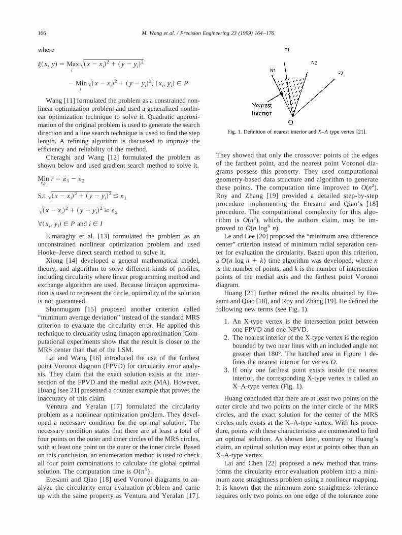![D

j~ x, y!

165M. Wang et al. / Precision Engineering 23 (1999) 164–176

where

j~ x, y! 5 Maxi

Î~ x 2 xi!2 1 ~ y 2 yi!

2

2 Mini

Î~ x 2 xi!2 1 ~ y 2 yi!

2, ~ xi, yi! [ P

Wang [11] formulated the problem as a constrained non-linear optimization problem and used a generalized nonlin-ear optimization technique to solve it. Quadratic approxi-mation of the original problem is used to generate the searchdirection and a line search technique is used to find the steplength. A refining algorithm is discussed to improve theefficiency and reliability of the method.

Cheraghi and Wang [12] formulated the problem asshown below and used gradient search method to solve it.

Minx,y

r 5 «1 2 «2

S.t.Î~ x 2 xi!2 1 ~ y 2 yi!

2 # «1

Î~ x 2 xi!2 1 ~ y 2 yi!

2 $ «2

@~ xi, yi! [ P and i [ I

Elmaraghy et al. [13] formulated the problem as anunconstrained nonlinear optimization problem and usedHooke–Jeeve direct search method to solve it.

Xiong [14] developed a general mathematical model,theory, and algorithm to solve different kinds of profiles,including circularity where linear programming method andexchange algorithm are used. Because limaçon approxima-tion is used to represent the circle, optimality of the solutionis not guaranteed.

Shunmugam [15] proposed another criterion called“minimum average deviation” instead of the standard MRScriterion to evaluate the circularity error. He applied thistechnique to circularity using limaçon approximation. Com-putational experiments show that the result is closer to theMRS center than that of the LSM.

Lai and Wang [16] introduced the use of the farthestpoint Voronoi diagram (FPVD) for circularity error analy-sis. They claim that the exact solution exists at the inter-section of the FPVD and the medial axis (MA). However,Huang [see 21] presented a counter example that proves theinaccuracy of this claim.

Ventura and Yeralan [17] formulated the circularityproblem as a nonlinear optimization problem. They devel-oped a necessary condition for the optimal solution. Thenecessary condition states that there are at least a total offour points on the outer and inner circles of the MRS circles,with at least one point on the outer or the inner circle. Basedon this conclusion, an enumeration method is used to checkall four point combinations to calculate the global optimalsolution. The computation time isO(n5).

Etesami and Qiao [18] used Voronoi diagrams to an-alyze the circularity error evaluation problem and cameup with the same property as Ventura and Yeralan [17].

They showed that only the crossover points of the edgesof the farthest point, and the nearest point Voronoi dia-grams possess this property. They used computationalgeometry-based data structure and algorithm to generatethese points. The computation time improved toO(n2).Roy and Zhang [19] provided a detailed step-by-stepprocedure implementing the Etesami and Qiao’s [18]procedure. The computational complexity for this algo-rithm is O(n2), which, the authors claim, may be im-proved toO(n log6 n).

Le and Lee [20] proposed the “minimum area differencecenter” criterion instead of minimum radial separation cen-ter for evaluation the circularity. Based upon this criterion,a O(n log n 1 k) time algorithm was developed, wherenis the number of points, andk is the number of intersectionpoints of the medial axis and the farthest point Voronoidiagram.

Huang [21] further refined the results obtained by Ete-sami and Qiao [18], and Roy and Zhang [19]. He defined thefollowing new terms (see Fig. 1).

1. An X-type vertex is the intersection point betweenone FPVD and one NPVD.

2. The nearest interior of the X-type vertex is the regionbounded by two near lines with an included angle notgreater than 180°. The hatched area in Figure 1 de-fines the nearest interior for vertexO.

3. If only one farthest point exists inside the nearestinterior, the corresponding X-type vertex is called anX–A-type vertex (Fig. 1).

Huang concluded that there are at least two points on theouter circle and two points on the inner circle of the MRScircles, and the exact solution for the center of the MRScircles only exists at the X–A-type vertex. With his proce-dure, points with these characteristics are enumerated to findan optimal solution. As shown later, contrary to Huang’sclaim, an optimal solution may exist at points other than anX–A-type vertex.

Lai and Chen [22] proposed a new method that trans-forms the circularity error evaluation problem into a mini-mum zone straightness problem using a nonlinear mapping.It is known that the minimum zone straightness tolerancerequires only two points on one edge of the tolerance zone

Fig. 1. Definition of nearest interior andX–A type vertex [21].

166 M. Wang et al. / Precision Engineering 23 (1999) 164–176

and one point on the other edge. This property contradictsHuang’s result [21] that there must exist at least two pointson the outer circle and two points on the inner circle of theMRS circles. Therefore, the Lai and Chen’s method doesnot guarantee optimal solution.

3. Mathematical Characterization and a SolutionAlgorithm

As defined previously, the circularity error evaluationproblem can be formulated as:

(M1)

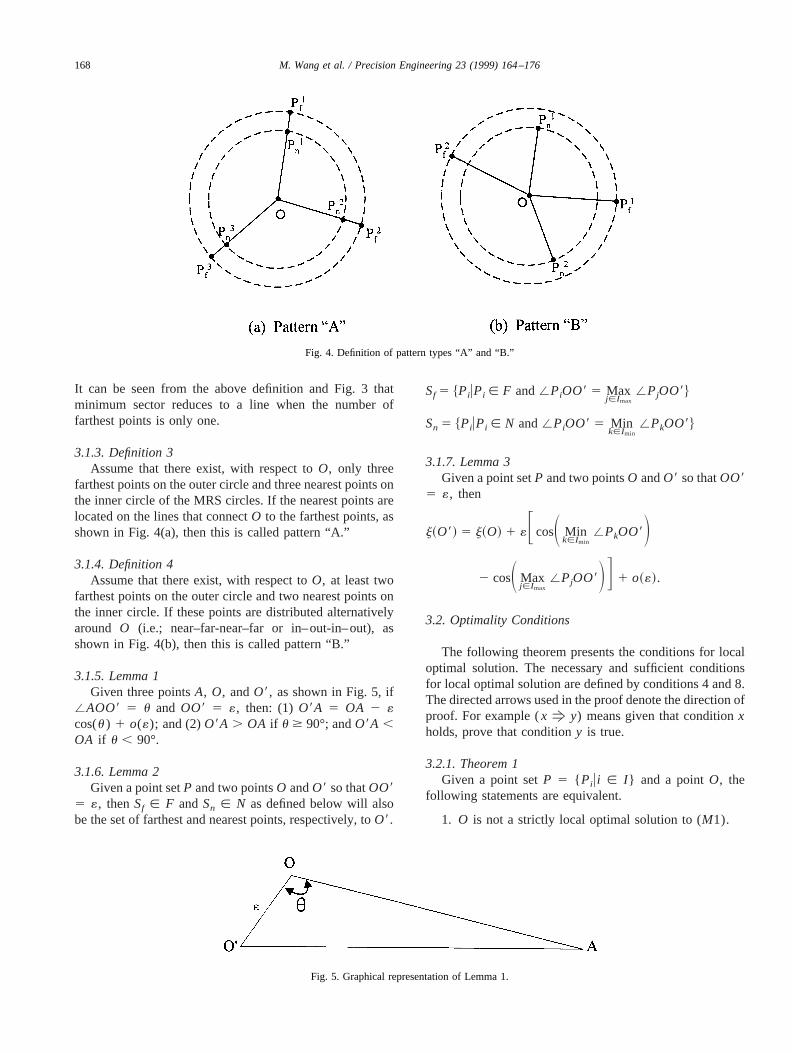
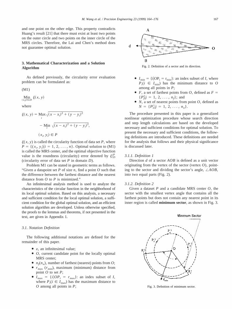
Min~ x,y![D

j~ x, y!

where

j~ x, y! 5 Maxi

Î~ x 2 xi!2 1 ~ y 2 yi!

2

2 Mini

Î~ x 2 xi!2 1 ~ y 2 yi!

2,

~ xi, yi! [ P

j( x, y) is called the circularity function of data setP, whereP 5 {( xi, yi)ui 5 1, 2, . . . ,n}. Optimal solution to (M1)is called the MRS center, and the optimal objective functionvalue is the roundness (circularity) error denoted byjuD

P

(circularity error of data setP in domainD).Problem M1 can be stated in geometric terms as follows.

“Given a datapoint setP of sizen, find a pointO such thatthe difference between the farthest distance and the nearestdistance fromO to P is minimized.”

An infinitesimal analysis method is used to analyze thecharacteristics of the circular function in the neighborhood ofits local optimal solution. Based on this analysis, a necessaryand sufficient condition for the local optimal solution, a suffi-cient condition for the global optimal solution, and an efficientsolution algorithm are developed. Unless otherwise specified,the proofs to the lemmas and theorems, if not presented in thetext, are given in Appendix 1.

3.1. Notation Definition

The following additional notations are defined for theremainder of this paper.

Y «, an infinitesimal value;Y O, current candidate point for the locally optimal

MRS center;Y nf(nn), number of farthest (nearest) points fromO;Y rmax (rmin), maximum (minimum) distance from

point O to setP;Y Imax 5 { i uOPi 5 rmax}: an index subset ofI ,

wherePi(i [ Imax) has the maximum distance toO among all points inP;

Y Imin 5 {i uOPi 5 rmin}: an index subset ofI , wherePi(i [ Imin) has the minimum distance toOamong all points inP;

Y F, a set of farthest points fromO, defined asF 5{ Pf

i uj 5 1, 2, . . . , nf}; andY N, a set of nearest points from pointO, defined as

N 5 { Pnj uj 5 1, 2, . . . , nn}.

The procedure presented in this paper is a generalizednonlinear optimization procedure whose search directionand step length calculations are based on the developednecessary and sufficient conditions for optimal solution. Topresent the necessary and sufficient conditions, the follow-ing definitions are introduced. These definitions are neededfor the analysis that follows and their physical significanceis discussed later.

3.1.1. Definition 1Direction d of a sectorAOB is defined as a unit vector

originating from the vertex of the sector (vertexO), point-ing to the sector and dividing the sector’s angle,/AOB,into two equal parts (Fig. 2).

3.1.2. Definition 2Given a datasetP and a candidate MRS centerO, the

sector with the smallest vertex angle that contains all thefarthest points but does not contain any nearest point in itsinner region is calledminimum sector, as shown in Fig. 3.

Fig. 2. Definition of a sector and its direction.

Fig. 3. Definition of minimum sector.


It can be seen from the above definition and Fig. 3 thatminimum sector reduces to a line when the number offarthest points is only one.

3.1.3. Definition 3Assume that there exist, with respect toO, only three

farthest points on the outer circle and three nearest points onthe inner circle of the MRS circles. If the nearest points arelocated on the lines that connectO to the farthest points, asshown in Fig. 4(a), then this is called pattern “A.”

3.1.4. Definition 4Assume that there exist, with respect toO, at least two

farthest points on the outer circle and two nearest points onthe inner circle. If these points are distributed alternativelyaround O (i.e.; near–far-near–far or in–out-in–out), asshown in Fig. 4(b), then this is called pattern “B.”

3.1.5. Lemma 1Given three pointsA, O, andO9, as shown in Fig. 5, if

/AOO9 5 u and OO9 5 «, then: (1)O9A 5 OA 2 «cos(u ) 1 o(«); and (2)O9A . OA if u $ 90°; andO9A ,OA if u , 90°.

3.1.6. Lemma 2Given a point setP and two pointsO andO9 so thatOO9

5 «, thenSf [ F andSn [ N as defined below will alsobe the set of farthest and nearest points, respectively, toO9.

Sf 5 $PiuPi [ F and/PiOO9 5 Maxj[Imax

/PjOO9%

Sn 5 $PiuPi [ N and/PiOO9 5 Mink[Imin

/PkOO9%

3.1.7. Lemma 3Given a point setP and two pointsO andO9 so thatOO9

5 «, then

j~O9! 5 j~O! 1 «F cosS Mink[Imin

/PkOO9D2 cosS Max

j[Imax/PjOO9DG 1 o~«!.

3.2. Optimality Conditions

The following theorem presents the conditions for localoptimal solution. The necessary and sufficient conditionsfor local optimal solution are defined by conditions 4 and 8.The directed arrows used in the proof denote the direction ofproof. For example (x f y) means given that conditionxholds, prove that conditiony is true.

3.2.1. Theorem 1Given a point setP 5 { Pi ui [ I } and a pointO, the

following statements are equivalent.

1. O is not a strictly local optimal solution to (M1).

Fig. 4. Definition of pattern types “A” and “B.”

Fig. 5. Graphical representation of Lemma 1.


2. There exists a feasible direction at pointO.3. Given any direction d, Maxj[Imax

(OPj∧d) #

Mink[Imin(OPk

∧d).4. There exists a sector that contains all the farthest

points with no nearest point in its inner region.5. Set

C 5 HxU OPj

iOPjiz x $

OPk

iOPkiz x,

x 5 ~x1, x2! [ R2, x Þ ~0, 0!, j [ Imaxand k [ IminJis not an empty set and contains all the feasibledirections.

6. The direction of the sector that contains all the far-thest points with no nearest point in its inner region isa feasible direction.

7. There exists a direction of the minimum sector.8. There does not exist a distribution of a subset of

farthest and nearest points showing patterns “A” or“B.”

3.2.2. Proof

1 f 2. BecauseO is not a strictly local optimal solution,there exists a feasible direction.

2 f 3. Assume that condition 3 does not hold, thenthere exists a direction vectord so that Maxj[Imax

(OPj∧d) . Mink[Imin

(OPk∧d). Select a pointO9 in

the direction ofd with an infinitesimal distance« fromO. Then from Lemma 3:

j~O9! 5 j~O! 1 « z F cos~ Mink[Imin

/PkOO9!

2 cosS Maxj[Imax

/PjOO9DG 1 o~«! . j~O!

So d is not a feasible direction, and condition 3 holds.

3 f 4. Because Maxj[Imax(OPj

∧d) # Mink[Imin

(OPk∧d), then a sector withO as its vertex,d as its

direction, and 2* Maxj[Imax(OPj∧d) as its vertex

angle, can be constructed, which contains all the far-thest points with no nearest point in its inner region.

4 f 5. Statement 5 is a mathematical representation of 4.5 f 6. Let d represent the direction of the sector that

contains all the farthest points with no nearest point inits inner region, then Maxj[Imax

(OPj∧d) # Mink[Imin

(OPk∧d). Thus

Maxj[Imax

S OPj

iOPji∧dD # Min

k[IminS OPk

iOPki∧dD ,

which meansOPj

iOPjiz d

$OPk

iOPkiz d for j [ Imax andk [ Imin

So d [ C and is a feasible direction.

6 f 7. Because the direction of the sector that containsall the farthest points with no nearest point in its innerregion is a feasible direction, then there exists a direc-tion of the minimum sector.

7 f 1. Because a feasible direction exists, thenO is nota strictly local optimal solution.

Conditions 4 and 8 are the necessary and sufficient con-ditions for local optimal solution.4 f 8. It can be observed from Fig 4 that, when there

exists a distribution of a subset of farthest points andnearest points showing pattern “A” or “B,” there doesnot exist a sector that contains all the farthest pointswith no nearest point in its inner region.

8 f 4. The following three cases are considered.

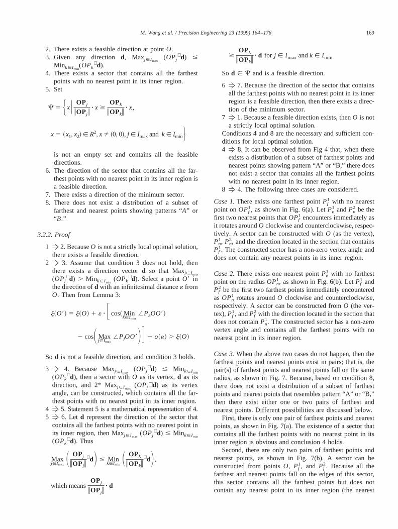
Case 1.There exists one farthest pointPf1 with no nearest

point onOPf1, as shown in Fig. 6(a). LetPn

1 andPn2 be the

first two nearest points thatOPf1 encounters immediately as

it rotates aroundO clockwise and counterclockwise, respec-tively. A sector can be constructed withO (as the vertex),Pn

1, Pn2, and the direction located in the section that contains

Pf1. The constructed sector has a non-zero vertex angle and

does not contain any nearest points in its inner region.

Case 2.There exists one nearest pointPn1 with no farthest

point on the radiusOPn1, as shown in Fig. 6(b). LetPf

1 andPf

2 be the first two farthest points immediately encounteredasOPn

1 rotates aroundO clockwise and counterclockwise,respectively. A sector can be constructed fromO (the ver-tex),Pf

1, andPf2 with the direction located in the section that

does not containPn1. The constructed sector has a non-zero

vertex angle and contains all the farthest points with nonearest point in its inner region.

Case 3.When the above two cases do not happen, then thefarthest points and nearest points exist in pairs; that is, thepair(s) of farthest points and nearest points fall on the sameradius, as shown in Fig. 7. Because, based on condition 8,there does not exist a distribution of a subset of farthestpoints and nearest points that resembles pattern “A” or “B,”then there exist either one or two pairs of farthest andnearest points. Different possibilities are discussed below.

First, there is only one pair of farthest points and nearestpoints, as shown in Fig. 7(a). The existence of a sector thatcontains all the farthest points with no nearest point in itsinner region is obvious and conclusion 4 holds.

Second, there are only two pairs of farthest points andnearest points, as shown in Fig. 7(b). A sector can beconstructed from pointsO, Pf

1, and Pf2. Because all the

farthest and nearest points fall on the edges of this sector,this sector contains all the farthest points but does notcontain any nearest point in its inner region (the nearest


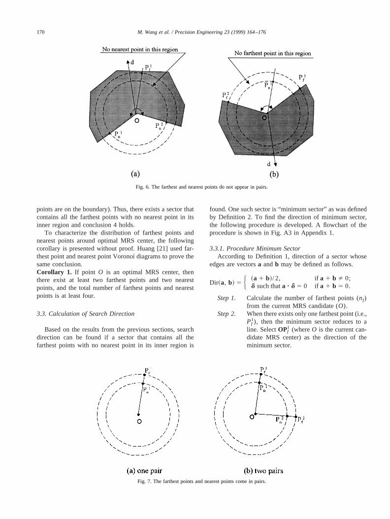
points are on the boundary). Thus, there exists a sector thatcontains all the farthest points with no nearest point in itsinner region and conclusion 4 holds.

To characterize the distribution of farthest points andnearest points around optimal MRS center, the followingcorollary is presented without proof. Huang [21] used far-thest point and nearest point Voronoi diagrams to prove thesame conclusion.Corollary 1. If point O is an optimal MRS center, thenthere exist at least two farthest points and two nearestpoints, and the total number of farthest points and nearestpoints is at least four.

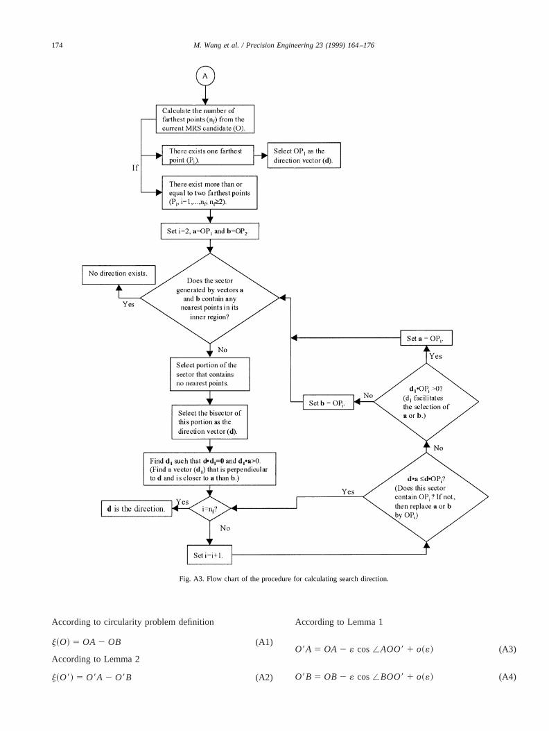
3.3. Calculation of Search Direction

Based on the results from the previous sections, searchdirection can be found if a sector that contains all thefarthest points with no nearest point in its inner region is

found. One such sector is “minimum sector” as was definedby Definition 2. To find the direction of minimum sector,the following procedure is developed. A flowchart of theprocedure is shown in Fig. A3 in Appendix 1.

3.3.1. Procedure Minimum SectorAccording to Definition 1, direction of a sector whose

edges are vectorsa andb may be defined as follows.

Dir~a, b! 5 H ~a 1 b!/ 2, if a 1 b Þ 0;d such thata ? d 5 0 if a 1 b 5 0.

Step 1. Calculate the number of farthest points (nf)from the current MRS candidate (O).

Step 2. When there exists only one farthest point (i.e.,Pf

1), then the minimum sector reduces to aline. SelectOPf

1 (whereO is the current can-didate MRS center) as the direction of theminimum sector.

Fig. 6. The farthest and nearest points do not appear in pairs.

Fig. 7. The farthest points and nearest points come in pairs.


Step 3. When there are only two farthest points (i.e.,Pf

1, Pf2), then letd 5 Dir(OPf

1, OPf2).

If (dzOPf1) $ Maxk[Imin

(dzOPk), thend isthe direction of the minimum sector.

Else if (dzOPf1) , Mink[Imin (dzOPk), then

(2d) is the direction of the minimum sector.Else there does not exist a direction of the

minimum sector.Step 4. When there exist more than two farthest

points (OPfi, i 5 1, . . . ,nf, nf . 2), leta 5

OPf1 andb 5 OPf

2. Set i 5 2.a. Use Step 3 to findd. If d does not exist,

then there does not exist a direction of theminimum sector; otherwise, find a direc-tion d1 such thatdzd1 5 0 andd1za . 0.

b. If i 5 nf output the direction, elsei 5i 1 1.

c. If (dza) # (dzOPfi), then go to b; other-

wise, continue.d. If (d1zOPf

i) . 0, then seta 5 OPfi; else

setb 5 OPfi. With the two new vectors

go to a.

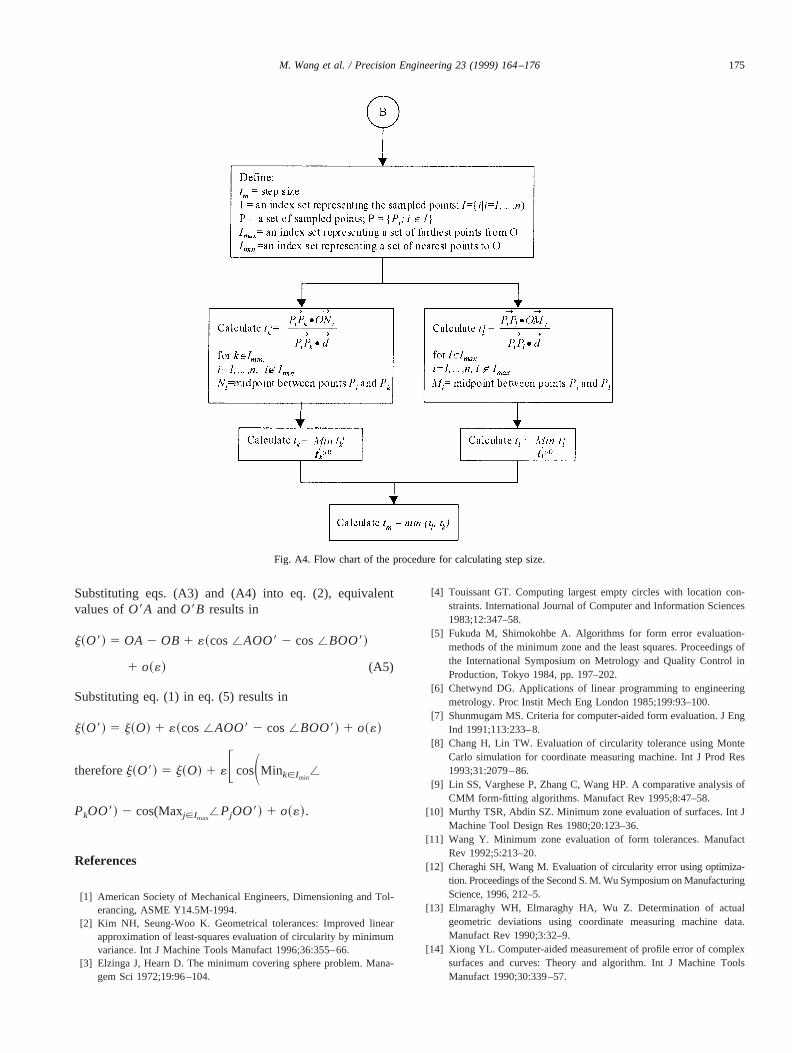
3.4. Step Length Calculation

To calculate step length, the following theorem is pre-sented.

3.4.1. Theorem 2Given a point setP, a good direction (unit vector)d, and

point O, the objective function value in (M1) will improveuntil either a new farthest point or a new nearest point isencountered. The step lengthtm is equal to the distance fromO to the new candidate MRS center,O9, where the first newfarthest point or nearest point is encountered. This can becalculated bytm 5 min{ tn, tf}, where tn represents thelength fromO to O9 where the first new nearest point isencountered. Also,tf defines the length fromO to O9, wherethe first new farthest point is encountered.

tn 5 Mintni .0

tni , wheretn

i 5PiPn ? ONi

PiPn ? d,

Ni is the middle point betweenPi andPn

tf 5 Mintfi.0

tfi, wheretf

i 5PiPf ? OM i

PiPf ? d,

Mi is the middle point betweenPi andPf.

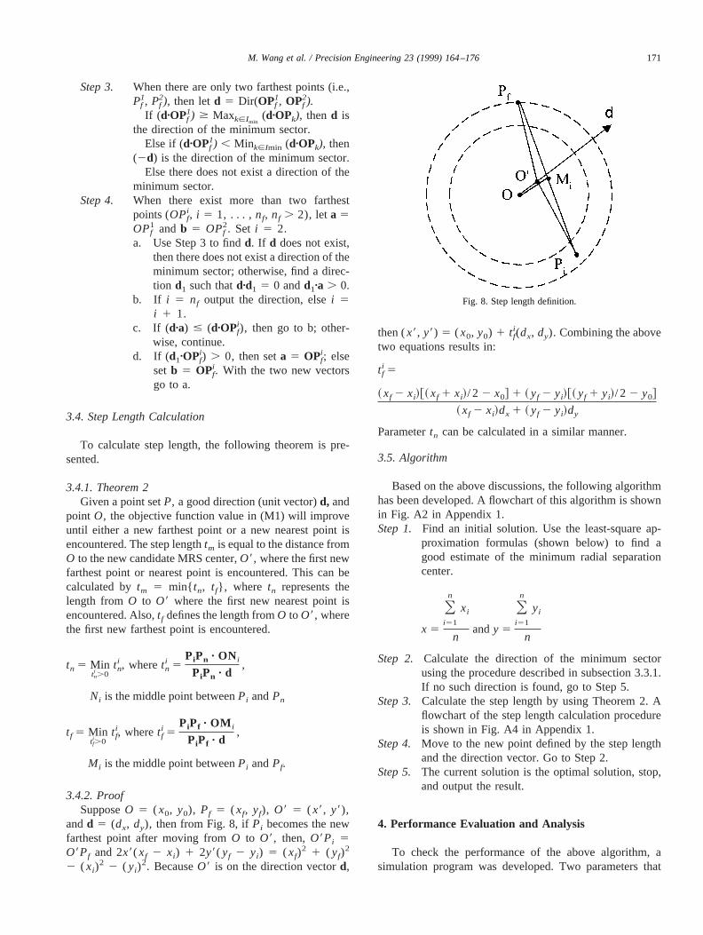
3.4.2. ProofSupposeO 5 ( x0, y0), Pf 5 ( xf, yf), O9 5 ( x9, y9),

andd 5 (dx, dy), then from Fig. 8, ifPi becomes the newfarthest point after moving fromO to O9, then, O9Pi 5O9Pf and 2x9( xf 2 xi) 1 2y9( yf 2 yi) 5 ( xf)

2 1 ( yf)2

2 ( xi)2 2 ( yi)

2. BecauseO9 is on the direction vectord,

then (x9, y9) 5 ( x0, y0) 1 tfi(dx, dy). Combining the above

two equations results in:

tfi 5

~ xf 2 xi!@~ xf 1 xi!/ 2 2 x0# 1 ~ yf 2 yi!@~ yf 1 yi!/ 2 2 y0#

~ xf 2 xi!dx 1 ~ yf 2 yi!dy

Parametertn can be calculated in a similar manner.

3.5. Algorithm

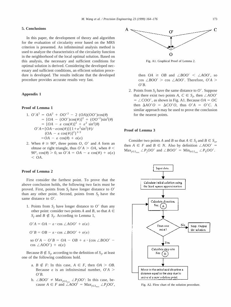
Based on the above discussions, the following algorithmhas been developed. A flowchart of this algorithm is shownin Fig. A2 in Appendix 1.Step 1. Find an initial solution. Use the least-square ap-

proximation formulas (shown below) to find agood estimate of the minimum radial separationcenter.

x 5

Oi51

n

xi

nandy 5

Oi51

n

yi

n

Step 2. Calculate the direction of the minimum sectorusing the procedure described in subsection 3.3.1.If no such direction is found, go to Step 5.

Step 3. Calculate the step length by using Theorem 2. Aflowchart of the step length calculation procedureis shown in Fig. A4 in Appendix 1.

Step 4. Move to the new point defined by the step lengthand the direction vector. Go to Step 2.

Step 5. The current solution is the optimal solution, stop,and output the result.

4. Performance Evaluation and Analysis

To check the performance of the above algorithm, asimulation program was developed. Two parameters that

Fig. 8. Step length definition.


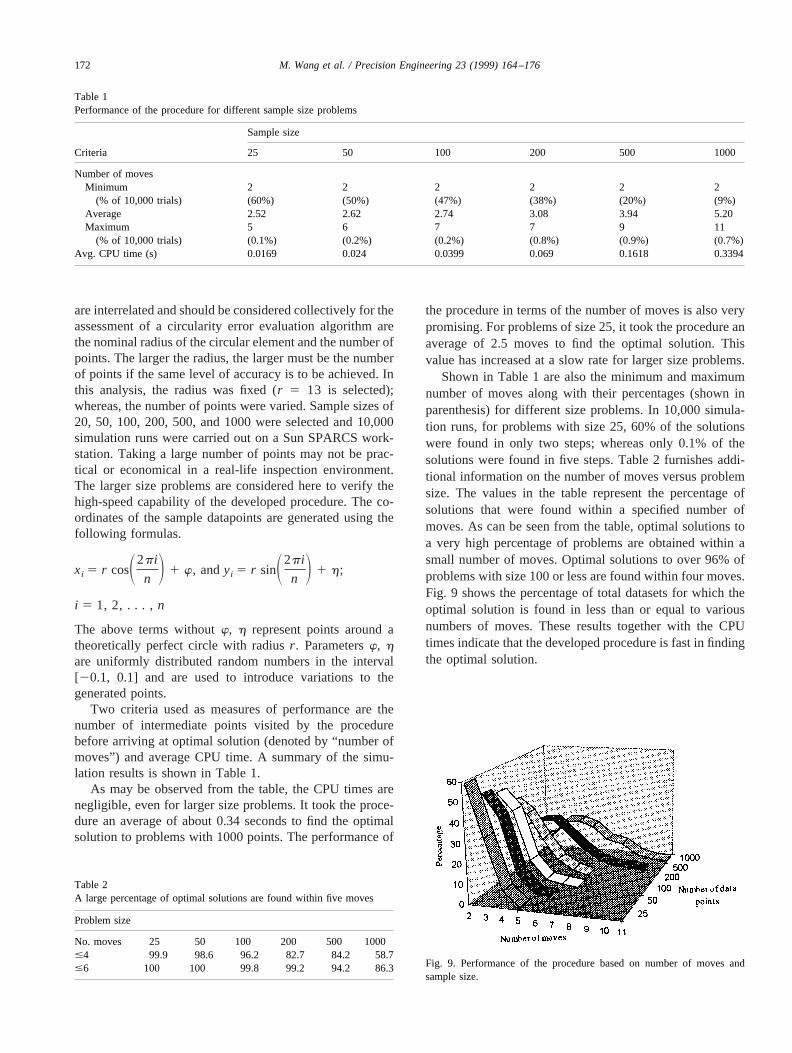
are interrelated and should be considered collectively for theassessment of a circularity error evaluation algorithm arethe nominal radius of the circular element and the number ofpoints. The larger the radius, the larger must be the numberof points if the same level of accuracy is to be achieved. Inthis analysis, the radius was fixed (r 5 13 is selected);whereas, the number of points were varied. Sample sizes of20, 50, 100, 200, 500, and 1000 were selected and 10,000simulation runs were carried out on a Sun SPARCS work-station. Taking a large number of points may not be prac-tical or economical in a real-life inspection environment.The larger size problems are considered here to verify thehigh-speed capability of the developed procedure. The co-ordinates of the sample datapoints are generated using thefollowing formulas.

xi 5 r cosS2pi

n D 1 w, andyi 5 r sinS2pi

n D 1 h;

i 5 1, 2, . . . ,n

The above terms withoutw, h represent points around atheoretically perfect circle with radiusr . Parametersw, hare uniformly distributed random numbers in the interval[20.1, 0.1] and are used to introduce variations to thegenerated points.

Two criteria used as measures of performance are thenumber of intermediate points visited by the procedurebefore arriving at optimal solution (denoted by “number ofmoves”) and average CPU time. A summary of the simu-lation results is shown in Table 1.

As may be observed from the table, the CPU times arenegligible, even for larger size problems. It took the proce-dure an average of about 0.34 seconds to find the optimalsolution to problems with 1000 points. The performance of

the procedure in terms of the number of moves is also verypromising. For problems of size 25, it took the procedure anaverage of 2.5 moves to find the optimal solution. Thisvalue has increased at a slow rate for larger size problems.

Shown in Table 1 are also the minimum and maximumnumber of moves along with their percentages (shown inparenthesis) for different size problems. In 10,000 simula-tion runs, for problems with size 25, 60% of the solutionswere found in only two steps; whereas only 0.1% of thesolutions were found in five steps. Table 2 furnishes addi-tional information on the number of moves versus problemsize. The values in the table represent the percentage ofsolutions that were found within a specified number ofmoves. As can be seen from the table, optimal solutions toa very high percentage of problems are obtained within asmall number of moves. Optimal solutions to over 96% ofproblems with size 100 or less are found within four moves.Fig. 9 shows the percentage of total datasets for which theoptimal solution is found in less than or equal to variousnumbers of moves. These results together with the CPUtimes indicate that the developed procedure is fast in findingthe optimal solution.

Fig. 9. Performance of the procedure based on number of moves andsample size.

Table 1Performance of the procedure for different sample size problems

Criteria

Sample size

25 50 100 200 500 1000

Number of movesMinimum 2 2 2 2 2 2

(% of 10,000 trials) (60%) (50%) (47%) (38%) (20%) (9%)Average 2.52 2.62 2.74 3.08 3.94 5.20Maximum 5 6 7 7 9 11

(% of 10,000 trials) (0.1%) (0.2%) (0.2%) (0.8%) (0.9%) (0.7%)Avg. CPU time (s) 0.0169 0.024 0.0399 0.069 0.1618 0.3394

Table 2A large percentage of optimal solutions are found within five moves

Problem size

No. moves 25 50 100 200 500 1000#4 99.9 98.6 96.2 82.7 84.2 58.7#6 100 100 99.8 99.2 94.2 86.3


5. Conclusions

In this paper, the development of theory and algorithmfor the evaluation of circularity error based on the MRScriterion is presented. An infinitesimal analysis method isused to analyze the characteristics of the circularity functionin the neighborhood of the local optimal solution. Based onthis analysis, the necessary and sufficient conditions foroptimal solution is derived. Considering the developed nec-essary and sufficient conditions, an efficient solution proce-dure is developed. The results indicate that the developedprocedure provides accurate results very fast.

Appendix 1

Proof of Lemma 1

1. O9A2 5 OA2 1 OO92 2 2 (OA)(OO9)cos(u)5 [OA 2 (OO9)cos(u )]2 1 (OO92)sin2(u)5 [OA 2 « cos(u )]2 1 «2 sin2(u)

O9A5[OA2«cos(u )]{1 1«2sin2(u )/(OA 2 « cos(u )]2} 1/ 2

5OA 2 « cos(u) 1 o(«)

2. Whenu $ 90°, three pointsO, O9 and A form anobtuse or right triangle, thusO9A . OA, whenu ,90°, cos(u) . 0, soO9A 5 OA 2 « cos(u ) 1 o(«), OA.

Proof of Lemma 2

First consider the farthest point. To prove that theabove conclusion holds, the following two facts must beproved. First, points fromSf have longer distance toO9than any other point. Second, points fromSf have thesame distance toO9.

1. Points fromSf have longer distance toO9 than anyother point: consider two pointsA andB, so thatA [Sf andB [y Sf. According to Lemma 1,

O9A 5 OA 2 « z cos/AOO9 1 o~«!

O9B 5 OB 2 « z cos/BOO9 1 o~«!

so O9A 2 O9B 5 OA 2 OB 1 « z (cos/BOO9 2cos /AOO9) 1 o(«)

BecauseB [y Sf, according to the definition ofSf, at leastone of the following conditions hold.

a. B [y F: In this case,A [ F, then OA . OB.Because« is an infinitesimal number,O9A .O9B.

b. /BOO9 Þ Maxj[Imax/PjOO9: In this case, be-

causeA [ F and /AOO9 5 Maxj[Imax/PjOO9,

then OA $ OB and /BOO9 , /AOO9, socos /BOO9 . cos /AOO9. Therefore,O9A .O9B.

2. Points fromSf have the same distance toO9. Supposethat there exist two pointsA, C [ Sf, then/AOO95 /COO9, as shown in Fig. A1. BecauseOA 5 OCthen DAO9O 5 DCO9O, thus O9A 5 O9C. Asimilar approach may be used to prove the conclusionfor the nearest points.

Proof of Lemma 3

Consider two pointsA andB so thatA [ Sf andB [ Sn,then A [ F and B [ N. Also by definition/AOO9 5Maxj[Imax

/PjOO9 and /BOO9 5 Mink[Imin/PkOO9.

Fig. A1. Graphical Proof of Lemma 2.

Fig. A2. Flow chart of the solution procedure.


According to circularity problem definition

j~O! 5 OA 2 OB (A1)

According to Lemma 2

j~O9! 5 O9A 2 O9B (A2)

According to Lemma 1

O9A 5 OA 2 « cos/AOO9 1 o~«! (A3)

O9B 5 OB 2 « cos/BOO9 1 o~«! (A4)

Fig. A3. Flow chart of the procedure for calculating search direction.


Substituting eqs. (A3) and (A4) into eq. (2), equivalentvalues ofO9A andO9B results in

j~O9! 5 OA 2 OB 1 «~cos/AOO9 2 cos/BOO9!

1 o~«! (A5)

Substituting eq. (1) in eq. (5) results in

j~O9! 5 j~O! 1 «~cos/AOO9 2 cos/BOO9! 1 o~«!

thereforej~O9! 5 j~O! 1 «F cosSMink[Imin/

PkOO9! 2 cos(Maxj[Imax/PjOO9! 1 o~«!.

References

[1] American Society of Mechanical Engineers, Dimensioning and Tol-erancing, ASME Y14.5M-1994.

[2] Kim NH, Seung-Woo K. Geometrical tolerances: Improved linearapproximation of least-squares evaluation of circularity by minimumvariance. Int J Machine Tools Manufact 1996;36:355–66.

[3] Elzinga J, Hearn D. The minimum covering sphere problem. Mana-gem Sci 1972;19:96–104.

[4] Touissant GT. Computing largest empty circles with location con-straints. International Journal of Computer and Information Sciences1983;12:347–58.

[5] Fukuda M, Shimokohbe A. Algorithms for form error evaluation-methods of the minimum zone and the least squares. Proceedings ofthe International Symposium on Metrology and Quality Control inProduction, Tokyo 1984, pp. 197–202.

[6] Chetwynd DG. Applications of linear programming to engineeringmetrology. Proc Instit Mech Eng London 1985;199:93–100.

[7] Shunmugam MS. Criteria for computer-aided form evaluation. J EngInd 1991;113:233–8.

[8] Chang H, Lin TW. Evaluation of circularity tolerance using MonteCarlo simulation for coordinate measuring machine. Int J Prod Res1993;31:2079–86.

[9] Lin SS, Varghese P, Zhang C, Wang HP. A comparative analysis ofCMM form-fitting algorithms. Manufact Rev 1995;8:47–58.

[10] Murthy TSR, Abdin SZ. Minimum zone evaluation of surfaces. Int JMachine Tool Design Res 1980;20:123–36.

[11] Wang Y. Minimum zone evaluation of form tolerances. ManufactRev 1992;5:213–20.

[12] Cheraghi SH, Wang M. Evaluation of circularity error using optimiza-tion. Proceedings of the Second S. M. Wu Symposium on ManufacturingScience, 1996, 212–5.

[13] Elmaraghy WH, Elmaraghy HA, Wu Z. Determination of actualgeometric deviations using coordinate measuring machine data.Manufact Rev 1990;3:32–9.

[14] Xiong YL. Computer-aided measurement of profile error of complexsurfaces and curves: Theory and algorithm. Int J Machine ToolsManufact 1990;30:339–57.

Fig. A4. Flow chart of the procedure for calculating step size.


[15] Shunmugam MS. New approach for evaluating form errors of engi-neering surfaces. Computer-Aided Design 1987;19:368–74.

[16] Lai Kewai, Wang J. A computational geometry approach to geomet-ric tolerancing. 16th North American Manufacturing Research Con-ference, University of Illinois, 1988, 376–9.

[17] Ventura JA, Yeralan S. The minimax center estimation problem forautomated roundness inspection. Euro J Op Res 1989;41:64–72.

[18] Etesami Faryar, Hong Q. Analysis of two-dimensional measure-ment data for automated inspection. J Manufact Syst 1990;9:21–34.

[19] Roy U, Zhang X. Establishment of a pair of concentric circles withthe minimum radial separation for assessing roundness error. Com-puter-Aided Design 1992;24:161–8.

[20] Le VB, Lee DT. Out-of-roundness problem revisited. IEEE Trans PattAnaly Machine Intelligence. 1991;13:217–23.

[21] Huang J. Evaluation of form and profile error in the measurement ofdiscrete parts. Ph.D. Diss, The Pennsylvania State University, Uni-versity Park, PA, 1994.

[22] Lai J, Chen I. Minimum zone evaluation of circles and cylinders. IntJ of Machine Tools and Manufacture 1996;36:435–51.


Documents

Circularity error evaluation