Christiansen Grammar for Some P Systems

Christiansen Grammar for Some P Systems

Alfonso Ortega de la Puente, Rafael Nunez Hervas,Marina de la Cruz Echeandıa, Manuel Alfonseca

Escuela Politecnica SuperiorDepartamento de Ingenierıa InformaticaUniversidad Autonoma de MadridCtra. de Colmenar km 15, 28049 Madrid, SpainE-mail: {alfonso.ortega, r.nunnez, marina.cruz, Manuel.Alfonseca}@uam.es

Summary. The main goal of this work is to formally describe P systems. This is anecessary step to subsequently apply Christiansen grammar evolution (an evolutionarytool developed by the authors) for automatic designing of P systems. Their complexstructure suggests us two decisions: to restrict our study to a subset of P systems thatease the representation while keeping a suitable complexity and to select a powerfulenough formal tool. Our work is restricted to a kind of P system that can simulate anylogical function by means of delay symbols and two mobile catalysts. Like in generalP systems, some components of these “logical” P systems depend on other components(for example, the number of axioms and regions and the set of possible indexes for thesymbols in their rules depend on the membrane structure). So, a formal representationable to handle context dependent constructions is needed. Our work uses Christiansengrammars to describe P systems.

1 Introduction

1.1 P systems

P Systems [7] are a kind of parallel and distributed computation model inspiredby the way in which cells process chemical compounds, energy and information.They can be briefly described as a collection of regions whose external membraneis called skin.

Each region in the model has four main components: a membrane that isolatesit from the rest of the P system, several symbols that are contained by it, produc-tion rules that describe the way in which these symbols can change and a set ofmembranes also contained by it.

The structure of the symbols contained by a membrane is called a multiset. Amultiset is a set in which multiple copies of each symbol are allowed. At each mo-ment, every region applies all its applicable production rules as much as possible.

230 A. Ortega de la Puente et al.

An order relationship, called priority ([8, 9]) can be used to solve the collisionsbetween rules applicable at the same moment in the same region.

Symbols can move across the membranes. That is, after applying a rule in aregion, some of its symbols can exit from the region or enter one of its directlyincluded regions.

Each kind of P system has a way to communicate the result of its computations.In this paper, a given region among those in the P system, called the output region,is used for this purpose.

Formal definition

P systems can be formally defined as follows.A P system of degree m ≥ 1 is the (2m + 4)-fold:

Π = (O, K, µ, ω0, . . ., ωm−1, (R0, ρ0), . . ., (Rm−1, ρm−1), io),

where:

• O is an alphabet. Its elements are called objects.• K ⊆ O is a distinguished subset of O, called the set of catalysts. These symbols

remain unchanged when they appear in a rule.• µ is a membrane structure with m membranes (usually labelled from 0 to

m− 1),• ωi, 0 ≤ i < m, specifies the initial multiset of the ith region.• Ri, 0 ≤ i < m, is the finite set of evolution rules for the ith region.• ρi is a partial order relation over Ri (the priority relation). Each evolution rule

joins two multisets of symbols. Subscripts {here, out, inj} are used to signalthe motion of the symbols across the membranes; here means no movement,out specifies that the symbol exits its region, and inj means that the symbolgoes into the jth region. This region must belong to the current membrane.Catalysts appear at most once in the left hand side of a rule and once in theright hand side. Catalysts can also be subscripted.

• io is the name of the output membrane. If io = −1, then the output is collectedfrom the environment.

1.2 P systems to compute logical functions

Reference [1] describes several ways in which P systems can simulate logical cir-cuits. They follow two steps: simulating a complete set of logical operands (suchas and, or, not) and designing a way to combine logical functions. One of theseapproaches simulates the basic logical operands by means of P systems with binaryalphabets ({0, 1}) extended by two mobile catalysts and some delay symbols. Thisis the approach used in this paper. Reference [1] contains a detailed descriptionand examples of the way in which this kind of P systems simulates any logicalfunction.

Christiansen Grammar for Some P Systems 231

1.3 Christiansen grammars

Christiansen grammars are an adaptable extension of attribute grammars in whichthe first attribute associated to every symbol is a Christiansen grammar. Likeattribute grammars, they have an ,universal computation power.

The first attribute of each non-terminal symbol contains the rules applicableto the corresponding symbol. Attributes are computed while the grammar is beingused, so it is possible to change the grammar on the fly.

This paper follows the same formal notation for Christiansen grammars [10],which uses, respectively, the symbols ↓ and ↑ before the name of inherited andsynthesized attributes.

2 Motivation

One of our main topics of interest is the formal specification of complex systemsthat makes it possible to apply formal tools to their design, or study some oftheir properties. Our research group has successfully applied this approach toother formal computational devices (L systems, cellular automata [5, 6, 2, 3])and proposed a new evolutionary automatic programming algorithm (Christiansengrammar evolution or CGE [4]) as a powerful tool to design complex systems tosolve specific tasks.

CGE wholly describes the candidate solutions, with Christiansen grammars,both syntactically and semantically, and hence, improves the performance of otherapproaches, because CGE reduces the search space by excluding non-promisingindividuals with syntactic or semantic errors.

P systems are abstract devices with a complex structure, because some of theircomponents depends on others (for example: the number of axioms and regionsand the set of proper suffixes to the right hand side of their evolution rules dependson the membrane structure µ). This dependence makes it difficult to use genetictechniques to search P systems because, in this circumstance, genetic operatorsusually produce a great number of incorrect individuals (both syntactically andsemantically).

This paper describes a first step to formally tackle the design of P systems.The next step will be to apply Christiansen grammar evolution to the design of Psystems.

As previously described, there are several ways of designing P systems to sim-ulate logic circuits. Each of these possibilities imposes some restrictions on P sys-tems, because it is not necessary to use the whole power of P systems to solve thisproblem.

This work is focused only on the formal description of these P systems. Itneither proposes any new technique to simulate logical functions nor improves thecomplexity of the approaches described in [1]. Our final goal is to test CGE fordesigning of P systems to solve the same task (to simulate any logical function)


and to compare both solutions. The evaluation of the results will be used in orderto propose a methodology to automatically design P systems.

3 Christiansen grammar for P systems that compute logicalfunctions

3.1 Informal description

A Christiansen grammar for P systems that compute logical functions must solvethe following situations:

• Every symbol of the alphabet (O), including catalysts, must be available to theset of rules of each region. So, the Christiansen grammar must have as manyattributes as needed to take this information into account.

• µ contains both the degree and the structure in the regions of the P system.The rules in the Christiansen grammar describing each region records thesedata by means of the attributes degree and daughters. The latter is a list of theregions that directly belong to it.

• Once a region is added to the system, the Christiansen grammar must add newsymbols to represent its axiom (w) and its rule set (Rnumber of region).

• An axiom is a multiset of symbols taken from O. Each evolution rule joins twomultisets. There are some constructions dependent on the context that dealwith the occurrence of catalysts:– A catalyst appears only once in a multiset. So, the semantic actions of the

rules in the Christiansen grammar that specify that a catalyst can belongto a multiset, must remove this possibility once the catalyst is derived.

– If a catalyst appears in the left hand side of a rule, it must also appearonce in the right hand side. So, the actions of the rules that describe aproduction rule of a region must force the occurrence of a catalyst to theright hand side only when it belongs to the left hand side. As stated in theprevious paragraph, our Christiansen grammar must forbid that a catalystappears more than once in a multiset.

• This paper handles multisets as strings. The order of the symbols in the stringsis not relevant: two strings that differ only in the order of their symbols areconsidered to be the same multiset.

3.2 Formal description

The Christiansen grammar proposed in this paper can be represented by thederivation rules formally described below.

1. ΠB{ ↓ g} → V { ↓ g, ↑ gV }C{ ↓ gV , ↑ gC}C ′{ ↓ gC , ↑ gC′}M{ ↓ gC′ , ↑ gM,}W{ ↓ gM}R{ ↓ gM}o{ ↓ gM},

where:


• ΠB stands for the whole P system.• V is the alphabet of the P system excluding the catalysts. It is convenient to

this paper that catalysts are considered apart from the rest of the alphabet. So,V will stand, throughout this work, for the alphabet excluding the catalysts.V changes the initial Christiansen grammar to record its symbols. The hardestwork deals with the delay symbols. The new grammar is synthesized by theattribute ↑ gV .

• C is the first catalyst and inherits from its left brother the current grammar(↓ gV ). When this catalyst is used, ↓ gV must be modified. The result is assignedas the synthesized value of ↑ gC .

• C ′ is the second catalyst. ↑ gC′ plays the same role as ↑ gC in the previoussymbol.

• M stands for the membrane structure.• W represents the axioms of the regions and inherits the changes from M .• R represents the rule sets of the regions. It is important to notice that R inherits

the current grammar from M rather than W because changes needed by eachaxiom are local to the axiom.

• o is the output region. It only needs to know the structure of M .

2. V { ↓ g, ↑ gV ∪ {SV { ↓ g} → 0|1}} → 01Sd{ ↓ g ↑ gV }.As previously described, P systems that compute logical functions are binary.

So{0, 1} ⊆ V.

In addition, several symbols (x′, x′′, . . . ) are used to synchronize the propaga-tion of data between different regions. They will be called delay symbols throughoutthis paper.

V contains 0, 1 and the delay symbols (represented by the non-terminal symbolSd).

Other components of the P system will access the symbols that belong to Vby means of the new non-terminal symbol SV .

Delay symbols are strings that begin with x followed by any amount (including0) of symbols “′”. Xd represents each delay symbol and Id its corresponding stringof “′”s, which is stored in its second attribute. Xd adds to the current grammar anew rule whose left hand side is Sd, providing further access to the derived delaysymbol.

3. Sd{ ↓ g, ↑ g} → λ,Sd{ ↓ g, ↑ gS} → Xd{ ↓ g ↑ gx}Sd{ ↓ gx ↑ gS},Xd{ ↓ g, ↑ g ∪ {SV { ↓ g} → x.string}} → xId{ ↓ g ↑ string},Id{ ↓ g, ↑ λ} → λ,Id{ ↓ g, ↑′ .string} →′ Id{ ↓ g, ↑ string},

4. C{ ↓ g, ↑ g ∪ {SC{ ↓ g, ↑ g} → c}} → c,C ′{ ↓ g, ↑ g ∪ {SC’{ ↓ g, ↑ g} → c′}} → c′,


where SC and SC′ are two new non-terminal symbols that represent respectivelythe catalysts c and c′. This P system uses at most two catalysts. Notice that unlikeSV , SC needs two attributes, because controlling the number of occurrences of eachcatalyst is a task that depends on the context. This task is accomplished by meansof the second attribute, and will be fully described further.

5. M{ ↓ g, ↑ gµ} → (µ{ ↓ g, ↑ gµ, ↓ degree = 0, ↑ degreeµ, ↑ daughters, ↓completed = yes}).M is a symbol to ensure that membrane structure is always contained in the

skin. µ, that appears in the right hand side of the following rule, is the mem-brane structure. Its last five attributes are used to keep the main changes neededby our Christiansen grammar. They will be described in detail in the followingparagraphs. The resulting grammar is the value synthesized for attribute ↑ gµ.

Notice that M does not modify the value synthesized by µ for its second at-tribute.

The membrane structure (µ) is a string of balanced parenthesis. µ is a maincomponent of ΠB since it determines its structure and the number of axioms andthe sets of rules needed. So the semantic actions of its rules make the biggestchanges to the grammar.

The following additional rules are involved in these changes:

6. w{ ↓ g, ↑ g} → λ,w{ ↓ g, ↑ g} → SV { ↓ g}w{ ↓ g},w{ ↓ g, ↑ gw} → SC{ ↓ g, ↑ gC =↓ g − {w → SCw}}w{ ↓ gC , ↑ gw},w{ ↓ g, ↑ gw} → SC’{ ↓ g, ↑ gC’ =↓ g − {w → SC’w}}w{ ↓ gC’, ↑ gw}.Each axiom is a string of symbols that belong to V (including λ). Catalysts are

also allowed but they can appear only once. This condition is accomplished in thesemantic actions of the third and fourth rule, that respectively remove w → SCwand w → SC′w from the grammar.

7. W{ ↓ g, ↑ g} → λ,R{ ↓ g, ↑ g} → λ.

Each time a new region is derived, a new axiom and a new region are respec-tively added to W and R. These new axioms and regions are concatenated to theright hand sides of their rules. So they are initially set to λ.

8. o{ ↓ g, ↑ g} → −1.

Each time a new region is derived, a new possible output region is added too. These new rules are added to the initial one, that represents the environment(−1).

9. Let j be degreeµ2 + 1(0).

µ{ ↓ g, ↑ gµ, ↓ degree, ↑ degreeµ2 + 1(0), ↑ daughtersµ1. ↑ degreeµ2, ↓ completed}→ µ1{ ↓ g, ↑ gµ1, ↓ degree, ↑ degreeµ1, ↑ daughtersµ1,↓ completed=no}


(µ2{ ↓ gµ1, ↑ gµ2, ↓ degreeµ1, ↑ degreeµ2,↑ daughters(↑ ), ↓ completed=yes}){if ↓ completed(5) equals to no, then ↑ gµ= ↑ gelse↑ gµ =↓ gµ2 ∪

{/∗These actions describe the region ↑ degreeµ2 whose daughters arecontained in ↑daughtersµ1.degreeµ2 ∗ /

W{ ↓ g} → right(W )(1).w{ ↓ g, ↑ }(2),o{ ↓ gR} → j,R{ ↓ g, ↑ g}→ right(R).Rj{ ↓ g, ↓ (production number)0, ↑ pn, },Rj{ ↓ g, ↓ pn, ↑ pn} → λ,Rj{ ↓ g, ↓ pn, ↑ pn2} → pj↓pn{ ↓ gp, ↓ pn + 1}R2

j{ ↓ g(3), ↓ pn + 1, ↑ pn2}{ Let k =↓ pn

and (6){r} = {pij,k → λ, pij,k → SCI’,j,k, pij,k → SCI,j,k,

pij,k → SCI,j,kSCI’,j,k, pij,k → SCI,j,kS

CI’,j,k}↓ gp =↓ g ∪ {

pj,k{ ↓ g, ↓ pn} → pdj,k{ ↓ g, ↑ gpd} → pij,k{ ↓ gpd, ↑ gpi},pdj,k{ ↓ g, ↑ g} → Sv{ ↓ g},pdj,k{ ↓ g, ↑ g} → Sv{ ↓ g}pdj,k{ ↓ g, ↑ g},pdj,k{ ↓ g, ↑ gpd} → SC{ ↓ g, ↑ gC =↓ g

− {pdj,k → SCpdj,k, pdj,k → SC}}pdj,k{ ↓ gC , ↑ gpd1}

{ ↑ gpd =↑ gpd1−{r}∪{pij,k{ ↓ g, ↑ g} → SCI,j,k{ ↓ g, ↑ g}.right(r)}}pdj,k{ ↓ g, ↑ gpd} → SC’{ ↓ g, ↑ gC’ =↓ g −

{pdj,k → SC’pdj,k, pdj,k → SC’}}pdj,k{ ↓ g

C’, ↑ gpd1}{ ↑ gpd =↑ gpd1−{r}∪{pij,k{ ↓ g, ↑ g} → S

CI’,j,k{ ↓ g ↑ g}.right(r)}}pdj,k{ ↓ g, ↑ gpd} → SC{ ↓ g, ↑ gC =↓ g

− {pdj,k → SCpdj,k, pdj,k → SC}}{ ↑ gpd =↑ gC −{r}∪{pij,k{ ↓ g, ↑ g} → SCI,j,k{ ↓ g, ↑ g}.right(r)}}

pdj,k{ ↓ g, ↑ gpd} → SC’{ ↓ g, ↑ g

C’ =↓ g− {pdj,k → SC’pdj,k, pdj,k → SC’}}

{ ↑ gpd =↑ gC’−{r}∪{pij,k{ ↓ g, ↑ g} → SCI’,j,k{ ↓ g, ↑ g}.right(r)}}SCI,j,k{ ↓ g, ↑ g} → ct : t ∈ {out, λ, inr, , r ∈↑ daughtersµ1.j}SCI’,j,k{ ↓ g, ↑ g} → c′t : t ∈ {out, λ, inr, , r ∈↑ daughtersµ1.j}pij,k{ ↓ g, ↑ g} → λ,pij,k{ ↓ g, ↑ gi} → s{ ↓ g}pij,k{ ↓ g, ↑ gi}s ∈ SV ∪{sd : s ∈ SV ∧d ∈ {out}∪{in.j : j ∈(4)↑ daughtersµ1.j}}}

}}

Most work is done when the regions are closed.


(a) The last five attributes of µ handles two properties of the membrane struc-ture:

• The degree or number of regions in the P system: the second and third at-tributes are used for this purpose. ↓degree inherits the current number of regionsthat initially equals 0, and the first rule (the one that closes each region) syn-thesizes the updated value (↑degreeµ2 +1), which is one more than the numberof regions accumulated by µ1 and µ2. This same value (↑degreeµ2 + 1) is thenumber of the current region and is used to identify it.

• The inclusion relationship between regions is contained in the penul-timate attribute (daughters), the list of the numbers of the regions directlyincluded by the just closed region. Notice that no deeper level is taken intoaccount, and notice too that to get the daughters of µ, it suffices to stick thenumber of the current region–1 to the daughters of µ1.

(b) New axioms and regions are added to the right hand sides of their corre-sponding rules (those whose left hand sides are respectively W and R).

(c) All the axioms can be described in the same way (w), but the rule set ofeach region depends on the structure of the region: the symbols to the right handsides of the rules can have as index the number of any of the regions that theydirectly include. So, a different non-terminal symbol (Rnum region) and a differentset of rules are used for each region.

(d) Not all the occurrences of µ must describe a region. One must do it onlywhen a region is really completed. The last attribute of µ (completed) takes intoaccount this circumstance. If the value of this attribute is no the grammar inheritedby µ remains unchanged. The reader can verify that, even if it closes a new regionby deriving the first rule, the first µ to the right hand side of the first rule cannotdescribe any region. Only the last µ really completes a region.

(e) Several conventions are used to simplify writing the preceding rules:

• j will be used rather than degreeµ2 + 1 to represent the number of the currentregion.

• All the attributes not used in their rules will be called . For example, ratherthan

µ2{ ↓ gµ1, ↑ gµ, ↓ degreeµ1, ↑ degreeµ2, ↑ daughters, ↓ completed}we will write

µ2{ ↓ gµ1, ↑ gµ, ↓ degreeµ1, ↑ degreeµ2, ↑ , ↓ completed},since the penultimate attribute of µ2 is not used in the rule. ↑daughters is notreally needed to compute the daughters of its father (the symbol µ at the lefthand side). The daughters of µ are only the regions that it includes at the firstlevel.


Additional notes

• (0)Notice that the number of the region described by these semantic actions isj = degreeµ2+1, which is the same as the degree synthesized; however, the valuesynthesized for daughters is daughtersµ1.degreeµ2 (so degreeµ2 = j − 1). It isvery important to “delay” the “propagation upwards” because the degree mustbe increased, to identify and describe the just closed region, after computingits list of daughters.

• (1)right(S), where S is a non-terminal symbol, is a function that returns theright hand side of the rule (there is at most one) in the grammar whose leftsymbol is S, or λ if there is no such rule.

• (2)The grammar synthesized by each axiom is not used, the key in this processis to keep the initial grammar independent of each axiom.

• (3) Changes made to the grammar by a production rule are local to the rule. Sopj↓pn and R2

j have the same grammar ↓ g as the value of their first attribute.• (4)“j ∈↑daughters” represents the set of symbols in the ↑daughters string.• (5) In these semantic actions, completed stands for the corresponding attribute

of the symbol µ at the left hand side, although the same name is used in theright hand side to simplify the notation.

• (6) Notice that, by construction, the set { pij,k → λ, pij,k → SCI’,j,k, pij,k →

SCI,j,k, pij,k → SCI,j,kSCI’,j,k, pij,k → SCI,j,kS

CI’,j,k } has only one element,and hence the expression {r} = {pij,k → λ, pij,k → SCI’,j,k, pij,k → SCI,j,k,pij,k → SCI,j,kS

CI’,j,k, pij,k → SCI,j,kSCI’,j,k} is correct.

10. µ{ ↓ g, ↑ gµ, ↓ degree, ↑ degree ↑ daughters = λ, ↓ completed} → λ{ if ↓completed equals to no then ↑ gµ= ↑ g

elseLet be j = degree

↑ gµ = {/*These actions describe the region ↑ degree that has nodaughters */W{ ↓ g} → right(W ).w{ ↓ g, ↑ }(5),

R{ ↓ g, ↑ g}→ right(R).Rj{ ↓ g, ↓ (production number) 0, ↑ pn, },Rj{ ↓ g, ↓ pn, ↑ pn} → λ,Rj{ ↓ g, ↓ pn, ↑ pn2} → pj↓pn{ ↓ gp, ↓ pn + 1}R2

j{ ↓ g, ↓ pn + 1, ↑ pn2}{Letk =↓ pnand{r} = {pij,k → λ, pij,k → S

CI’,j,k, pij,k → SCI,j,k,

pij,k → SCI,j,kSCI’,j,k, pij,k → SCI,j,kSCI’,j,k}↓ gp =↓ g ∪ {

pj,k{ ↓ g, ↓ pn} → pdj,k{ ↓ g, ↑ gpd} → pij,k{ ↓ gpd, ↑ gpi},pdj,k{ ↓ g, ↑ g} → Sv{ ↓ g},pdj,k{ ↓ g, ↑ g} → Sv{ ↓ g}pdj,k{ ↓ g, ↑ g},pdj,k{ ↓ g, ↑ gpd} → SC{ ↓ g, ↑ gC =↓ g

− {pdj,k → SCpdj,k, pdj,k → SC}}


pdj,k{ ↓ gC , ↑ gpd1}{ ↑ gpd =↑ gpd1−{r}∪{pij,k{ ↓ g, ↑ g} → SCI,j,k{ ↓ g, ↑ g}.right(r)}}

pdj,k{ ↓ g, ↑ gpd} → SC’{ ↓ g, ↑ gC’ =↓ g −{pdj,k → S

C’pdj,k, pdj,k → SC’}}

pdj,k{ ↓ gC’, ↑ gpd1}

{ ↑ gpd =↑ gpd1−{r}∪{pij,k{ ↓ g, ↑ g} → SCI’j,k{ ↓ g, ↑ g}.right(r)}}

pdj,k{ ↓ g, ↑ gpd} → SC{ ↓ g, ↑ gC =↓ g− {pdj,k → SCpdj,k, pdj,k → SC}}

{ ↑ gpd =↑ gC−{r}∪{pij,k{ ↓ g, ↑ g} → SCI,j,k{ ↓ g, ↑ g}.right(r)}}pdj,k{ ↓ g, ↑ gpd} → SC’{ ↓ g, ↑ gC’ =↓ g

− {pdj,k → SC’pdj,k, pdj,k → SC’}}{ ↑ gpd =↑ g

C’−{r}∪{pij,k{ ↓ g, ↑ g} → SCI’,j,k{ ↓ g, ↑ g}.right(r)}}

SCI,j,k{ ↓ g, ↑ g} → ct : t ∈ {out, λ}SCI’,j,k{ ↓ g, ↑ g} → c′t : t ∈ {out, λ}pij,k{ ↓ g, ↑ g} → λ,pij,k{ ↓ g, ↑ gi} → s{ ↓ g}pij,k{ ↓ g, ↑ gi}

, , s ∈ SV ∪ {sd : s ∈ SV ∧ d ∈ {out}}o{ ↓ gR} → j}

}}

Notice that the semantic actions of this rule are very similar to the previousone. This rule describes an empty region (↑ daughters = λ), so its symbols canonly remain in the region (without any index) or exit from it (by using out as theindex).

3.3 Example

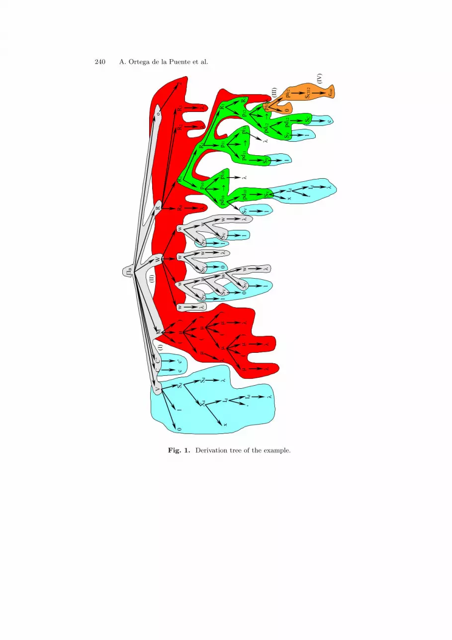
Figure 1 shows a derivation tree for the P systemΠB = (V = {0, 1, x′}, C = {c, c′}, µ = ((()0()1)2)3, ω0 = λ, ω1 = 101, ω2 =

0, ω3 = 11,

(R0 = ∅, ρ0 = ∅),(R1 = {

p10 = 1x′ → λ,p11 = 1 → λ,

p12 = 1c → cout0}

, ρ1 = {p10 ≥ p11 ≥ p12}),(R2 = ∅, ρ2 = ∅),(R3 = ∅, ρ3 = ∅),

io = 2).

Some information will not be explicitly represented:


• The correspondence between axioms and regions will be deduced from theirpositions: so, the jth axiom will belong to the region Rj−1 (notice that theindex of the regions is zero based).

• The order relationship for the rules of a region is determined by their appear-ance order.

The derivation process will be briefly described. The tree in Figure 1 shows thederivation tree of this P system. Different colors are used to remark some circum-stances that help to understand how our Christiansen grammar works:

• Color gray highlights the information that is known from the beginning of theprocess (the structures of ΠB , and the axioms). Hence, these derivation rulesbelong to the initial grammar.

• Color blue indicates the information that depends on the derived alphabet(specially the subset of delay symbols). The rules that describe non-terminalsymbols SV , Sd, SC and SC’ are added to the grammar after deriving the sym-bols V , C and C ′.

• M (the membrane structure) is the main component of the P system becauseit determines the number of regions (the degree) and their structure. So, it ismandatory to finish the derivation of M before adding to the grammar thederivation rules that describe the number of axioms and regions and the basicstructure of each region as a set of production rules. Color red designates thisdependence.

• Each region records the number of its rules. Each rule is described by threenon-terminal symbols (one for its left hand side, one for its right hand sideand another one for the complete rule) that are identified by two indices j, k(corresponding to the kth rule of the jth region). So, it is impossible to add thederivation rules for these three non-terminals after deriving the region itself.Color green highlights this situation.

• Finally, the structure to the right hand side of the rules depends on the left handside because of the catalysts. So, the description of the right hand sides in thegrammar can be modified after deriving the left hand sides. This dependenceis emphasized with color orange.

We will highlight the most significant steps in the derivation of this example:

• (I) After specifying the complete alphabet.• (II) After processing the membrane structure.• (III) After describing R1 (except pi1,2 the right hand side of its last rule p1,2).• (IV) After finishing the P system.

The first rule applied is

1. ΠB{↓ g} → V {↓ g, ↑ gV }C{ ↓ gV , ↑ gC}C ′{ ↓ gC , ↑ gC’}

M{ ↓ gC’, ↑ gM}W{ ↓ gM}R{ ↓ gM}o{ ↓ gM}.V inherits its first attribute from ΠB .When the rule


PB

VC

m

WR

o

c0

1S

d

Sd

Xd I d

x

I d‘

l

mm

()

mm

()

lm

m(

)

l

ll

l

ww

w

wS

Vw

SV

wS

V

wS

Vw

SV

wS

V

1

0

01

1l

1l

2R

1R

3 lR

1p

10

R1

p11

R1

p12

pi 1

0pd

10

pi 1

1pd

11

pi 1

2pd

12

l

SV 1

SV 1

pd

12

1

c

l

C’

c'

l®

®

®l

R2 l

pd

10

SV

I d‘

l

I dx

()

M

R0

l

w l

SV

SC

pi 1

20

SC

I12

c out

(I)

(II)

(III

)

(IV

)

Fig. 1. Derivation tree of the example.


2. V {↓ g, ↑ gV ∪ {SV { ↓ g} → 0|1}} → 01Sd{↓ g ↑ gV }is applied, Sd inherits the value of its first attribute from V . Sd must synthesizeits second attribute before V can add the rules SV { ↓ g} → 0|1 to it.

Figure 2 graphically shows the evaluation of ↑ gV and its modification by thesemantic actions of the previous rule. Red arrows are used to highlight synthesis,while blue arrows represent inheritance. The modifications to the current grammarare shown between brackets.

Sd

SdXd

Idx

Id‘

l

l

l

‘

x‘ {SV{¯g}®x’} {SV{¯g}®x.string}

{SV{¯g}®x’}

V

0 1

{SV{¯g}®0|1|x’}

‘.l=’

Fig. 2. Derivation tree after applying the rule number 2.

At this moment the rule

1. ΠB{↓ g} → V {↓ g, ↑ gV}C{↓ g

V, ↑ gC}C ′{ ↓ gC , ↑ gC’}

M{ ↓ gC’, ↑ gM}W{ ↓ gM}R{ ↓ gµ}o{ ↓ gµ}

can be revisited, because symbol V has finished the evaluation of its attributes andC can inherit the value of its first attribute from V . Figure 3 graphically showsthe computation of the attributes while applying the rules

4. C{ ↓ g, ↑ g ∪ {SC{ ↓ g, ↑ g} → c}} → cC ′{ ↓ g, ↑ g ∪ {S

C’{ ↓ g, ↑ g} → c′}} → c′.

After finishing the evaluation of the attributes of C ′, the remaining substringto the right hand side of the first rule can be processed.

1. ΠB{↓ g, ↑ gR} → V {↓ g, ↑ gV}C{↓ g

V, ↑ g

C}C ′{↓ g

C, ↑ g

C′} (0)

M{↓ gC′

, ↑ gM}W{ ↓ gM}R{ ↓ gM}o{ ↓ gM}.


V C

c

C’

c'

{SV{¯g}®0|1|x’} {SV{¯g}®0|1|x.’,

SC{¯g, g}®c }

{SV{¯g}®0|1|x.’,

SC{¯g, g}®c,

SC’{¯g, g}®c’ }

Fig. 3. Derivation tree after applying the rule number 4.

The non-terminal M inherits the value of its first attribute from C ′.The only rule applicable to M is

5. M{↓ g =↓ gC′

, ↑ gM =↑ gµ} → (µ{ ↓ g, ↑ gµ,↓ degree = 0, ↑ degreeµ, ↑daughters,↓ completed = yes}).Notice that M only inherits its first attribute. M will synthesize its last at-

tribute after processing µ.The next step will determine the structure of the P system and make the major

changes to the grammar. Figure 4 graphically shows the result of the process.Once µ is fully derived, we can continue with M . Its second attribute does not

modify the second one for the symbol µ to the right hand side.

M{↓ g, ↑ gµ= (d)} → (µ{↓ g, ↑ g

µ= (d), ↓0, ↑ degree

µ2+1 = 3,

↑ daughtersµ1

.degreeµ2

=2, ↓completed=yes}).Now it is possible to process W (the axioms of the regions of ΠB), which is the

next symbol in expression (0), that inherits (d) from M has its initial grammar.Expression (0′) updates the attributes of µ and W . Notice that R and o can alsoevaluate their initial grammars to (d).

ΠB{↓ g, ↑ gR} → V{↓ g, ↑ gV } C{↓gV , ↑gC} C’{↓gC , ↑gC′}M{↓gC′ , ↑gµ=(d)}(0’)W{↑gµ=(d)} R{↑gµ=(d), ↑gR}o{↑ gµ=(d)}

Grammar (d) has only one rule applicable to W

7. W{↓g=(d)}→ {↓g=(d),↑ }w{↓g=(d),↑ }w{↓g=(d),↑ }w{↓g=(d),↑ }

No change is made to the initial grammar. The reader can verify in the initialderivation tree that each axiom is derived by means of pure context free mecha-nisms.

At this point, we process symbol R.Grammar (d) has only a rule applicable to R.

R{↓g=(d) }→ R0{↓g=(d),↓0, ↑ pn }


m

m m( )

m

m m( )

ll

l

{SV{¯g}®0|1|x.’,

SC{¯g, g}®c,

SC’{¯g, g}®c’},

(d),

0, 3,

2, yes{SV{¯g}®0|1|x.’,

SC{¯g, g}®c,

SC’{¯g, g}®c’ }

{SV{¯g}®0|1|x.’,

SC{¯g, g}®c,

SC’{¯g, g}®c’ },

0, 0,

l, no

{SV{¯g}®0|1|x.’,

SC{¯g, g}®c,

SC’{¯g, g}®c’ }

(c),

0, 2,

0.1, yes

{SV{¯g}®0|1|x’,

SC{¯g, g}®c,

SC’{¯g, g}®c’ }

{SV{¯g}®0|1|x’,

SC{¯g, g}®c,

SC’{¯g, g}®c’ },

0, 0,

l, no

{SV{¯g}®0|1|x.’,

SC{¯g, g}®c,

SC’{¯g, g}®c’ }

(a),

0,1,

0, no

{SV{¯g}®0|1|x’,

SC{¯g, g}®c,

SC’{¯g, g}®c’ }

(a),

0, 0,

l, yes

m( )

l

(c)

(d)(a),

(b),

1,1,

l,yes

(a)

M

( )

{SV{¯g}®0|1|x’,

SC{¯g, g}®c,

SC’{¯g, g}®c’ },

-

(b)

(c)={ SV{¯g}®0|1|x’, SC{¯g, g}®c, SC’{¯g, g}®c’,

W{¯g}®w{¯g, _ }w{¯g, _ }, o{¯gR}®-1|0|1|2

R{¯g,g}®R0{¯g, _ ,¯0, pn } R1{¯g, _ ,¯0, pn } R2{¯g, _ ,¯0, pn },

R0{¯g, g, ¯pn, pn}®l,

R0{¯g, _,¯pn, pn2}®p0¯pn{¯gp,¯pn+1}R02{¯g, gR, ¯pn+1, pn2}{···}

R1{¯g, g, ¯pn, pn}®l,


R2{¯g, g, ¯pn, pn}®l,


}

(d)= { SV{¯g}®0|1|x’, SC{¯g, g}®c, SC’{¯g, g}®c’,

W{¯g}®w{¯g, _ }w{¯g, _ } w{¯g, _ } w{¯g, _ }, o{¯gR}®-1|0|1|2|3

R{¯g }®R0{¯g, ¯0,pn }R1{¯g, ¯0, pn }

R2{¯g, ¯0,pn }R3{¯g, ¯0, pn },

R0{¯g, ¯pn, pn}®l,

R0{¯g, ¯pn, pn2}®p0¯pn{¯gp,¯pn+1}R02{¯g, ¯pn+1, pn2}{···}

R1{¯g, ¯pn, pn}®l,


R2{¯g, ¯pn, pn}®l,


R3{¯g, ¯pn, pn}®l,


}

Fig. 4. Derivation tree after processing µ.


R1{↓g=(d), ↓0, ↑ pn }R2{↓g=(d), ↓0, ↑ pn }R3{↓g=(d), ↓0, ↑ pn }

It is worth noticing that each region does not depend on the other regions. Theyinherit the initial grammar from R and use 0 as the initial number of productionrules.

The last eight rules in grammar (d)describe R0, R1, R2 and R3 as sets of 0 ormore production rules. Each production rule has two indices that identify it (jand k). So pj,k is the kth rule for the jth region.

Grammar (d), however, does not describe each production rule. The semanticactions of the following rules modify and complete (d):

R0{ ↓ g, ↓ pn, ↑ pn2} → p0↓pn{ ↓ gp, ↓ pn + 1}R20{ ↓ g, ↓ pn + 1, ↑ pn2}{ · · · }




The following paragraphs explain this process.Three of the four regions (R0, R2 and R3) are empty. The subtree in figure 5

corresponds to region R1.Rule R1{ ↓ g, ↓ pn, ↑ pn2} → p1↓pn{ ↓ gp, ↓ pn+1}R2

1{ ↓ g, ↓ pn+1, ↑ pn2}{···}is initially applied to symbol R1{↓ g = (d), ↓ 0, ↑ pn }. Expression (g) shows thissituation.

R1{↓g=(d), ↓0,↑ pn2} →(g)p10{↓gp=(e),↓pn+1=0+1=1}R2

1{↓g=(d), ↓ pn + 1 = 0 + 1 = 1,↑ pn2}{ Let {r} = {pi1,0 → λ, pi1,0 → S

CI’,1,0, pi1,0 → SCI,1,0,

pi1,0 → SCI,1,0SCI′,1,0, pi1,0 → SCI,1,0SCI′,1,0 }↓gp=(e)=(d) ∪ {

p1,0{↓g, ↓pn}→pd1,0 {↓g, ↑gpd} →pi1,0 {↓gpd, ↑gpi},pd1,0 {↓g, ↑g}→Sv{↓g},pd1,0 {↓g, ↑g}→Sv{↓g}pd1,0 {↓g, ↑g},pd1,0 {↓g,↑gpd}→SC{↓g,↑gC=↓g

-{pd1,0 →SCpd1,0,pd1,0 →SC}}pd1,0 {↓gC, ↑gpd1}

{↑gpd=↑gpd1-{r}∪{pi1,0{↓g,↑g}→SCI,1,0{↓g↑g}.right(r)}}pd1,0 {↓g, ↑gpd}→SC {↓g,↑gC′=↓g-

{pd1,0 →SC′pd1,0, pd1,0 →SC′}}pd1,0 {↓gC′, ↑gpd1}

{↑gpd=↑gpd1-{r}∪{pi1,0{↓g,↑g}→SCI′,1,0{↓g↑g}.right(r)}}pd1,0 {↓g, ↑gpd}→ SC{↓g,↑gC=↓g

-{ pd1,0 →SCpd1,0, pd1,0 →SC}}{↑gpd=↑gC-{r}∪{pi1,0{↓g,↑g}→SCI,1,0{↓g↑g}.right(r)}}


R1

R1p10

R1p11

R1p12

pi10pd10

pi11pd11

pd12 l

SV

1 SV

1 SV pd12

1 SV

c

l

®

®

®l

pd10

SV

Id‘

l

Idx

pi12

pi120

SCI12

cout

Fig. 5. Subtree of region R1.

pd1,0 {↓g, ↑gpd}→ SC′{↓g,↑gC′=↓g-{ pd1,0 →SC′pd1,0, pd1,0 →SC′}}

{↑gpd=↑gC′-{r}∪{pi1,0{↓g,↑g}→SCI′,1,0{↓g↑g}.right(r)}}SCI,1,0 {↓g, ↑g}→ct:t∈{out, λ }SCI′,1,0 {↓g, ↑g}→c’ t:t∈{out, λ }pi1,0 {↓g, ↑g}→ λ,pi1,0 {↓g, ↑g i }→s{↓g} pi1,0 {↓g, ↑g i }, s∈SV ∪{sd: s∈SV ∧ d∈{out}}}

}Notice that these semantic actions have two main purposes: to compute the

number of production rules of the region to be used as the second index of thecorresponding non terminal symbols (pjk) and to complete the grammar with thedefinition of pdj,k and pij,k that represent respectively the left and right hand sidesof the production rules.

Figure 6 shows the derivation tree before modifying the grammar to force thecatalyst to appear in the right hand side of p1,2.

Figure 7 shows the grammars (i) and (h).


R1

R1p10

R1p11

R1p12

pi10pd10

pi11pd11

pi12pd12 l

SV

1 SV

1 SV pd12

1 SC

c

l

®

®

®l

pd10

SV

Id‘

l

Idx

(d),

_, 0, -

(e),

1

(d),

_, 1, -

(e),

(e)

(e),

(e)

(f),

2

(d),

_, 2, -

(g),

(i)

(g),

(h)

(g),

(i)

(i),

-

pi120

SCI12

cout

Fig. 6. Derivation tree before processing pi1,2.

Notice that (i), that becomes the initial grammar for pi1,2, has replaced

pi1,2{ ↓ g, ↑ g} → λ

bypi1,2{ ↓ g, ↑ gi} → SCI,1,2{ ↓ g, ↑ g}.

Given that pi1,2{ ↓ g, ↑ g} → λ was the only way to finish the process of thenon-terminal pi1,2 (its other rules are recursive), (i) ensures that SCI,1,2 appearsexactly once in the last derivation associated to pi1,2, and hence (after finishingpi1,2 the complete process of rule p1,2 also finishes) it is unnecessary to modify thegrammar to force that non-terminal SCI,1,2does not appear again.

The last rule applied to derive the output region (o → 2) is one of the possi-bilities included by (i) and finishes the derivation of the example.

4 Conclusions and future research

This paper uses Christiansen grammars to formally describe an interesting kindof P systems, those that simulate logical functions by means of delay symbols andtwo mobile catalysts. In this way, our work suggests a formal description of P


(h)={ SV{¯g}®0|1|x’, SC{¯g, g}®c, SC’{¯g, g}®c’,

W{¯g}®w{¯g, _ }w{¯g, _ } w{¯g, _ } w{¯g, _ }, o{¯gR}®-1|0|1|2|3

R{¯g }®R0{¯g, ¯0,pn }R1{¯g, ¯0, pn }

R2{¯g, ¯0,pn }R3{¯g, ¯0, pn },

R0{¯g, ¯pn, pn}®l,


R1{¯g, ¯pn, pn}®l,

R1{¯g, ¯pn, pn2}®p1¯pn{¯gp,¯pn+1}R12{¯g, ¯pn+1, pn2}

p 1,2 {¯g, ¯pn}®pd1,2 {¯g, gpd} ®pi1,2 {¯gpd, gpi},

pd 1,2 {¯g, g}®Sv{¯g},

pd 1,2 {¯g, g}®Sv{¯g}pd1,2 {¯g, g},

pd 1,2 {¯g, gpd}®SC’ {¯g,gC’=¯g-{pd1,2 ®SC’pd1,2, pd1,2 ®SC’}}pd1,2 {¯gC’, gpd1}{···}

pd 1,2 {¯g, gpd}® SC’{¯g,gC’=¯g-{ pd1,2 ®SC’pd1,2, pd1,2 ®SC’}}{···}

S CI,1,2 {¯g, g}®ct:tÎ{out, l }

S CI’,1,2 {¯g, g}®c’t:tÎ{out, l }

pi 1,2 {¯g, g}® l,

pi1,2 {¯g, gi }®s{¯g} pi1,2 {¯g, gi },, sÎSVÈ{sd: sÎSVÙ dÎ{out}}

R2{¯g, ¯pn, pn}®l,


R3{¯g, ¯pn, pn}®l,


}

(i)={ SV{¯g}®0|1|x’, SC{¯g, g}®c, SC’{¯g, g}®c’,

W{¯g}®w{¯g, _ }w{¯g, _ } w{¯g, _ } w{¯g, _ }, o{¯gR}®-1|0|1|2|3

R{¯g }®R0{¯g, ¯0,pn }R1{¯g, ¯0, pn }

R2{¯g, ¯0,pn }R3{¯g, ¯0, pn },

R0{¯g, ¯pn, pn}®l,


R1{¯g, ¯pn, pn}®l,

R1{¯g, ¯pn, pn2}®p1¯pn{¯gp,¯pn+1}R12{¯g, ¯pn+1, pn2}

p 1,2 {¯g, ¯pn}®pd1,2 {¯g, gpd} ®pi1,2 {¯gpd, gpi},

pd 1,2 {¯g, g}®Sv{¯g},

pd 1,2 {¯g, g}®Sv{¯g}pd1,2 {¯g, g},

pd 1,2 {¯g, gpd}®SC’ {¯g,gC’=¯g-{pd1,2 ®SC’pd1,2, pd1,2 ®SC’}}pd1,2 {¯gC’, gpd1}{···}

pd 1,2 {¯g, gpd}® SC’{¯g,gC’=¯g-{ pd1,2 ®SC’pd1,2, pd1,2 ®SC’}}{···}

S CI,1,2 {¯g, g}®ct:tÎ{out, l }

S CI’,1,2 {¯g, g}®c’t:tÎ{out, l }

pi1,2{¯g,gi}®SCI,1,2{¯g,g},

pi 1,2 {¯g, gi }®s{¯g} pi1,2 {¯g, gi },, sÎSVÈ{sd: sÎSVÙ dÎ{out}}

R2{¯g, ¯pn, pn}®l,


R3{¯g, ¯pn, pn}®l,


}

Fig. 7. Grammars of Figure 6.


systems constructions. In fact, it seems possible to use the techniques proposedin this work to translate the hierarchy of the components of any P system intoChristiansen grammar mechanisms.

Our future work will extend this paper in the following lines:

• This proposal will be used in the automatic design of P systems that simulatelogical functions by means of CGE (Christiansen grammar evolution).

• Christiansen grammars (and CGE) will be applied to other types of P systems,even to P systems without restrictions.

References

1. R. Ceterchi, D. Sburlan: Simulating Boolean circuits with P systems. MembraneComputing, International Workshop, WMC 2003. Tarragona, Spain, July, 17-22,2003, Revised Papers, LNCS 2933, Springer-Verlag, Berlin, 2004, 104–122.

2. A.L.A. Dalhoum, A. Ortega, M. Alfonseca: Cellular automata equivalent to PD0Lsystems. Proc. of International Arab Conference on Information Technology (ACIT2003), December 20-23, 2003, Alexandria, Egypt, 819–825.

3. A.L.A. Dalhoum, A. Ortega, M. Alfonseca: Cellular automata equivalent to D0Lsystems. 3rd WSEAS International Conference on Systems Theory and ScientificComputation, Special Session on Cellular Automata and Applications, November 15-17, 2003, Rodas, Greece.

4. A. Ortega, M. Cruz Echeandıa, M. Alfonseca: Christiansen grammar evolution:Grammatical evolution with semantic. Submitted, 2004.

5. A. Ortega, A.L.A. Dalhoum, M. Alfonseca: Grammatical evolution to design fractalcurves with a given dimension. IBM Jr. of Res. and Dev. (SCI JCR 2.560), 47, 4(2003), 483–493.

6. A. Ortega, A.L.A. Dalhoum, M. Alfonseca: Cellular automata equivalent to DILSystems. Proc. of 5th Middle East Symposium on Simulation and Modelling (MESM2003), Eurosim, January 5-7, 2004, Sharjah, United Arabic Emirates, 120–124.

7. Gh. Paun: Computing with membranes. An introduction. Bulletin of the EATCS, 68(February 1999), 139–152.

8. Gh. Paun: Computing with membranes. Journal of Computer and Systems Sciences,61, 1 (2000), 108–143.

9. Gh. Paun: Computing with membranes: Attacking NP-complete problems. Uncon-ventional models of Computation, UMC’2K, Bruxelles, 2000, 94–115.

10. J.N. Shutt: Recursive Adaptable Grammars. A thesis submitted to the Faculty of theWorcester Polytechnic Institute in partial fulfilment of the requirements for the de-gree of Master of Science in Computer Science. August 10, 1993 (enmended December16, 2003).

Documents

Christiansen Grammar for Some P Systems