Embed Size (px)
Citation preview
Chemistry Climate Model Simulations of Polar
Stratospheric Ozone
by
Matthias Brakebusch
M.Sc., Leibniz Universitat Hannover, 2007
M.Sc., University of Colorado at Boulder, 2011
A thesis submitted to the
Faculty of the Graduate School of the
University of Colorado in partial fulfillment
of the requirements for the degree of
Doctor of Philosophy
Department of Atmospheric and Oceanic Sciences
2013
This thesis entitled:Chemistry Climate Model Simulations of Polar Stratospheric Ozone
written by Matthias Brakebuschhas been approved for the Department of Atmospheric and Oceanic Sciences
Prof. Cora E. Randall
Dr. V. Lynn Harvey
Date
The final copy of this thesis has been examined by the signatories, and we find that both thecontent and the form meet acceptable presentation standards of scholarly work in the above
mentioned discipline.

iii
Brakebusch, Matthias (Ph.D., Atmospheric Science)
Chemistry Climate Model Simulations of Polar Stratospheric Ozone
Thesis directed by Prof. Cora E. Randall
Stratospheric ozone (O3) plays a crucial role in protecting organisms on Earth from lethal
shortwave solar radiation. Because it is radiatively active, O3 also determines the temperature
structure of the stratosphere, so its distribution affects the circulation. For these reasons, under-
standing polar stratospheric O3 has been a high priority of the scientific community for decades. Of
primary interest in recent years is explaining and predicting variations in O3 in a changing climate.
Stratospheric O3 distributions are affected by both chemistry and transport, which in turn are
controlled by temperature, circulation, and dynamics. Hence, investigations of polar stratospheric
O3 require the separation of these intertwined processes, and an understanding of the relevant
feedbacks. Investigations of these processes require global observations as well as coupled chem-
istry climate model simulations. This thesis focuses on chemical O3 loss due to halogen and odd
nitrogen (NOX) catalytic cycles, and utilizes satellite measurements from several instruments and
the Specified Dynamics Whole Atmosphere Community Climate Model (SD-WACCM).
The science questions are: (1) Is SD-WACCM a tool sophisticated enough for quantitative O3
evolution investigations? (2) How much O3 loss can be accurately attributed to the stratospheric
O3 loss processes induced by halogens, energetic particle precipitation, and NOX individually? (3)
Why is the observed O3 in the Arctic 2010/2011 winter exceptionally low, despite high dynamical
variability, which is usually associated with less O3 loss?
The questions are addressed by: (1) iteratively evaluating and improving SD-WACCM simula-
tions of the Arctic 2004/2005 winter through comparisons with satellite observations; (2) comparing
multiple experimental SD-WACCM simulations of the Antarctic 2005 winter omitting individual
O3 loss processes to a reference simulation; (3) testing a hypothesis by means of a comprehensive
model simulation of the Arctic 2010/11 winter season.

iv
Conclusions of this thesis are: (1) SD-WACCM is a useful tool to quantify polar stratospheric
O3 evolution after including several model improvements; (2) 74% of total column O3 loss can be
attributed robustly to halogen chemistry preceded by heterogeneous chemistry; (3) severe O3 loss
in Arctic 2010/11 results in part from enhanced chlorine activation due to the high dynamical
variability.
The work of this thesis improved SD-WACCM and adds an unprecedented evaluation re-
garding O3 variability and O3 loss in the stratosphere. Exact quantification of individual O3 loss
processes became possible even for extreme seasons. Hence this thesis enables analyses of polar
stratospheric winter seasons on a level of detail that was not possible before.
v
Acknowledgements
I gratefully acknowledge my advisor Cora Randall. In addition to financial support, she made
this thesis possible through numerous meetings, discussions, suggestions, language corrections, and
personal advice. Many thanks also go to my committee members, who were always available for
discussions and suggestions. In particular I thank Doug Kinnison who took me on the long and
winding road through the modeling world. From a distance, Michelle Santee and Gloria Manney
were a tremendous help with their invaluable feedback on my work.
Everyone in the middle atmosphere group was available for discussions, chat, and coffee which
made the work on my PhD project quite a bit more interactive. I thank Bodil Karlsson in particular
for bringing a new perspective into my view and planting a seed called Stockholm. I especially have
to express my gratitude to Laura Holt as a group member but mostly as a friend and for sharing
thoughts on many levels.
For clearing my mind in my spare time I’d like to thank Sam Stevenson and Steve Davis,
especially for dragging me along into the beauty of Colorado. For reminding me of the Gemutlichkeit
”back home” and being wonderful friends I’m grateful to Simone Stahringer and Jochen Wendel.
Although far away, thank you to Benjamin Ruprecht who is always there for listening, thinking
along, second opinions, and whole new insights.
I’m grateful for my understanding and loving family who all of a sudden saw me around
Christmas time only. Above all I express my gratitude to my partner Susanne Benze who was
always on my side during the sunniest and darkest moments of this entire journey; and who taught
me to always look forward to our next joint chapter.

vi
Contents
Chapter
1 Introduction 1
2 Polar Stratospheric Ozone 6
2.1 Polar Stratospheric Dynamics . . . . . . . . . . . . . . . . . . . . . . . . . . . . . . . 9
2.1.1 Brewer Dobson Circulation . . . . . . . . . . . . . . . . . . . . . . . . . . . . 9
2.1.2 Polar Vortex . . . . . . . . . . . . . . . . . . . . . . . . . . . . . . . . . . . . 11
2.1.3 Hemispheric Differences (Dynamics) . . . . . . . . . . . . . . . . . . . . . . . 13
2.2 Polar Stratospheric Chemistry . . . . . . . . . . . . . . . . . . . . . . . . . . . . . . 14
2.2.1 Photochemistry . . . . . . . . . . . . . . . . . . . . . . . . . . . . . . . . . . . 15
2.2.2 Gas-Phase Catalytic Chemistry . . . . . . . . . . . . . . . . . . . . . . . . . . 17
2.2.3 Polar Stratospheric Clouds . . . . . . . . . . . . . . . . . . . . . . . . . . . . 23
2.2.4 Energetic Particle Precipitation . . . . . . . . . . . . . . . . . . . . . . . . . . 27
2.2.5 Hemispheric Differences (Chemistry) . . . . . . . . . . . . . . . . . . . . . . . 29
2.3 Investigation of Polar Stratospheric Ozone . . . . . . . . . . . . . . . . . . . . . . . . 29
2.4 Science Questions . . . . . . . . . . . . . . . . . . . . . . . . . . . . . . . . . . . . . . 32
3 SD-WACCM simulations of the Arctic winter 2004/05 36
3.1 Evaluation of Whole Atmosphere Community Climate Model simulations of ozone
during Arctic winter 2004-2005 . . . . . . . . . . . . . . . . . . . . . . . . . . . . . . 37
3.1.1 Introduction . . . . . . . . . . . . . . . . . . . . . . . . . . . . . . . . . . . . 38

vii
3.1.2 Method . . . . . . . . . . . . . . . . . . . . . . . . . . . . . . . . . . . . . . . 40
3.1.3 Model/Measurement Comparisons . . . . . . . . . . . . . . . . . . . . . . . . 46
3.1.4 Discussion . . . . . . . . . . . . . . . . . . . . . . . . . . . . . . . . . . . . . . 60
3.1.5 Summary and Conclusions . . . . . . . . . . . . . . . . . . . . . . . . . . . . . 67
4 SD-WACCM simulations of the Antarctic winter 2005 70
4.1 Introduction . . . . . . . . . . . . . . . . . . . . . . . . . . . . . . . . . . . . . . . . . 71
4.2 Method . . . . . . . . . . . . . . . . . . . . . . . . . . . . . . . . . . . . . . . . . . . 73
4.3 Evaluation Results . . . . . . . . . . . . . . . . . . . . . . . . . . . . . . . . . . . . . 75
4.3.1 Temperature . . . . . . . . . . . . . . . . . . . . . . . . . . . . . . . . . . . . 76
4.3.2 Ozone . . . . . . . . . . . . . . . . . . . . . . . . . . . . . . . . . . . . . . . . 78
4.3.3 Transport . . . . . . . . . . . . . . . . . . . . . . . . . . . . . . . . . . . . . . 78
4.3.4 Halogen Chemistry . . . . . . . . . . . . . . . . . . . . . . . . . . . . . . . . . 79
4.3.5 PSC Formation . . . . . . . . . . . . . . . . . . . . . . . . . . . . . . . . . . . 79
4.3.6 Upper Atmosphere . . . . . . . . . . . . . . . . . . . . . . . . . . . . . . . . . 82
4.4 Ozone Loss Attribution Results . . . . . . . . . . . . . . . . . . . . . . . . . . . . . . 83
4.4.1 Dynamical Feedback . . . . . . . . . . . . . . . . . . . . . . . . . . . . . . . . 84
4.4.2 Ozone Loss Attribution . . . . . . . . . . . . . . . . . . . . . . . . . . . . . . 85
4.5 Conclusions . . . . . . . . . . . . . . . . . . . . . . . . . . . . . . . . . . . . . . . . . 88
5 SD-WACCM simulations of the Arctic winter 2010/11 90
5.1 Introduction . . . . . . . . . . . . . . . . . . . . . . . . . . . . . . . . . . . . . . . . . 90
5.2 Hypothesis . . . . . . . . . . . . . . . . . . . . . . . . . . . . . . . . . . . . . . . . . 91
5.3 Method . . . . . . . . . . . . . . . . . . . . . . . . . . . . . . . . . . . . . . . . . . . 93
5.4 Evaluation Results . . . . . . . . . . . . . . . . . . . . . . . . . . . . . . . . . . . . . 94
5.4.1 Temperature . . . . . . . . . . . . . . . . . . . . . . . . . . . . . . . . . . . . 94
5.4.2 Ozone . . . . . . . . . . . . . . . . . . . . . . . . . . . . . . . . . . . . . . . . 96
5.4.3 Transport . . . . . . . . . . . . . . . . . . . . . . . . . . . . . . . . . . . . . . 96
viii
5.4.4 Halogen Chemistry . . . . . . . . . . . . . . . . . . . . . . . . . . . . . . . . . 97
5.4.5 PSC Formation . . . . . . . . . . . . . . . . . . . . . . . . . . . . . . . . . . . 98
5.5 Partitioning results . . . . . . . . . . . . . . . . . . . . . . . . . . . . . . . . . . . . . 98
6 Conclusions and Outlook 101
6.1 Conclusions . . . . . . . . . . . . . . . . . . . . . . . . . . . . . . . . . . . . . . . . . 101
6.2 Contributions . . . . . . . . . . . . . . . . . . . . . . . . . . . . . . . . . . . . . . . . 103
6.2.1 Technical contributions . . . . . . . . . . . . . . . . . . . . . . . . . . . . . . 103
6.2.2 Contributions to science . . . . . . . . . . . . . . . . . . . . . . . . . . . . . . 104
6.3 Future Plans . . . . . . . . . . . . . . . . . . . . . . . . . . . . . . . . . . . . . . . . 108
6.3.1 Additional analysis for the NH 2010/11 study . . . . . . . . . . . . . . . . . . 108
6.3.2 Identified but unresolved model deficiencies . . . . . . . . . . . . . . . . . . . 108
6.3.3 Experiment about hypothetical extreme SPEs . . . . . . . . . . . . . . . . . . 109
Bibliography 111
Appendix
A Gridding Method 123
B Initialization Method 125
C Averaging Method 127
D Satellite History File 129
E Workflow 131
List of Acronyms 132
List of Chemical Species 136
ix
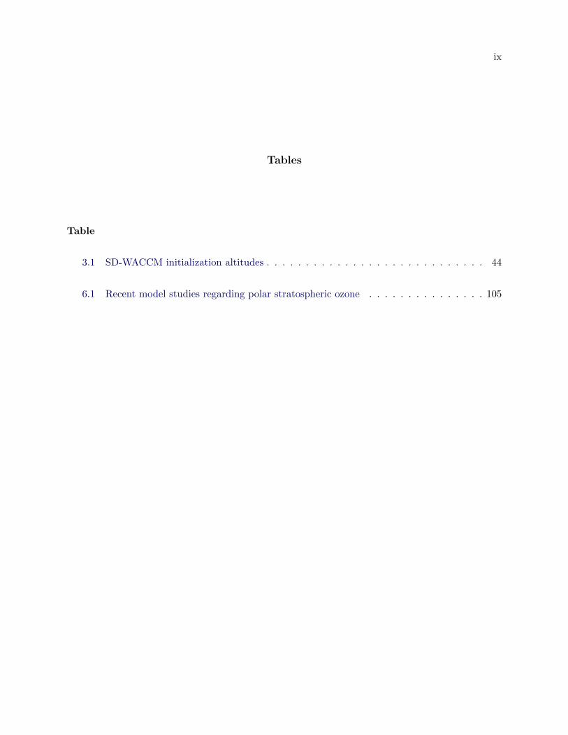
Tables
Table
3.1 SD-WACCM initialization altitudes . . . . . . . . . . . . . . . . . . . . . . . . . . . . 44
6.1 Recent model studies regarding polar stratospheric ozone . . . . . . . . . . . . . . . 105
x
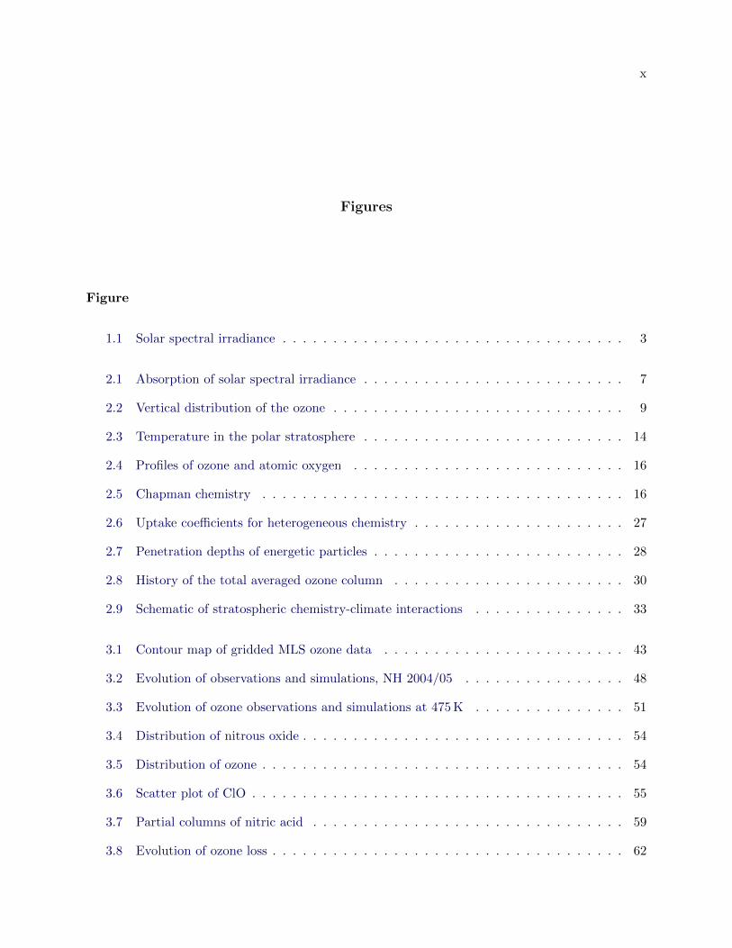
Figures
Figure
1.1 Solar spectral irradiance . . . . . . . . . . . . . . . . . . . . . . . . . . . . . . . . . . 3
2.1 Absorption of solar spectral irradiance . . . . . . . . . . . . . . . . . . . . . . . . . . 7
2.2 Vertical distribution of the ozone . . . . . . . . . . . . . . . . . . . . . . . . . . . . . 9
2.3 Temperature in the polar stratosphere . . . . . . . . . . . . . . . . . . . . . . . . . . 14
2.4 Profiles of ozone and atomic oxygen . . . . . . . . . . . . . . . . . . . . . . . . . . . 16
2.5 Chapman chemistry . . . . . . . . . . . . . . . . . . . . . . . . . . . . . . . . . . . . 16
2.6 Uptake coefficients for heterogeneous chemistry . . . . . . . . . . . . . . . . . . . . . 27
2.7 Penetration depths of energetic particles . . . . . . . . . . . . . . . . . . . . . . . . . 28
2.8 History of the total averaged ozone column . . . . . . . . . . . . . . . . . . . . . . . 30
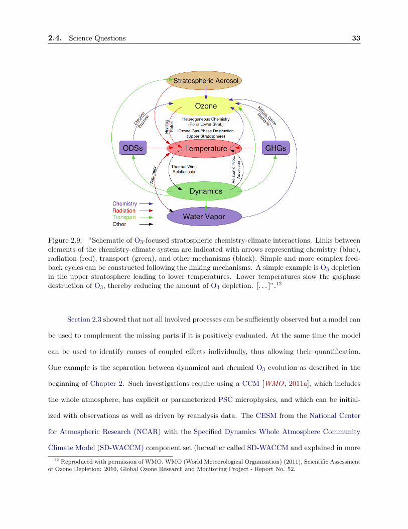
2.9 Schematic of stratospheric chemistry-climate interactions . . . . . . . . . . . . . . . 33
3.1 Contour map of gridded MLS ozone data . . . . . . . . . . . . . . . . . . . . . . . . 43
3.2 Evolution of observations and simulations, NH 2004/05 . . . . . . . . . . . . . . . . 48
3.3 Evolution of ozone observations and simulations at 475 K . . . . . . . . . . . . . . . 51
3.4 Distribution of nitrous oxide . . . . . . . . . . . . . . . . . . . . . . . . . . . . . . . . 54
3.5 Distribution of ozone . . . . . . . . . . . . . . . . . . . . . . . . . . . . . . . . . . . . 54
3.6 Scatter plot of ClO . . . . . . . . . . . . . . . . . . . . . . . . . . . . . . . . . . . . . 55
3.7 Partial columns of nitric acid . . . . . . . . . . . . . . . . . . . . . . . . . . . . . . . 59
3.8 Evolution of ozone loss . . . . . . . . . . . . . . . . . . . . . . . . . . . . . . . . . . . 62
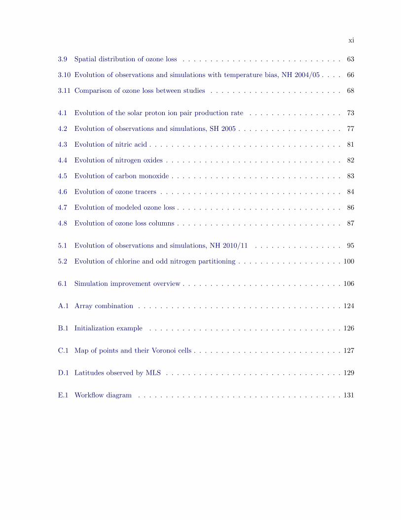
xi
3.9 Spatial distribution of ozone loss . . . . . . . . . . . . . . . . . . . . . . . . . . . . . 63
3.10 Evolution of observations and simulations with temperature bias, NH 2004/05 . . . . 66
3.11 Comparison of ozone loss between studies . . . . . . . . . . . . . . . . . . . . . . . . 68
4.1 Evolution of the solar proton ion pair production rate . . . . . . . . . . . . . . . . . 73
4.2 Evolution of observations and simulations, SH 2005 . . . . . . . . . . . . . . . . . . . 77
4.3 Evolution of nitric acid . . . . . . . . . . . . . . . . . . . . . . . . . . . . . . . . . . . 81
4.4 Evolution of nitrogen oxides . . . . . . . . . . . . . . . . . . . . . . . . . . . . . . . . 82
4.5 Evolution of carbon monoxide . . . . . . . . . . . . . . . . . . . . . . . . . . . . . . . 83
4.6 Evolution of ozone tracers . . . . . . . . . . . . . . . . . . . . . . . . . . . . . . . . . 84
4.7 Evolution of modeled ozone loss . . . . . . . . . . . . . . . . . . . . . . . . . . . . . . 86
4.8 Evolution of ozone loss columns . . . . . . . . . . . . . . . . . . . . . . . . . . . . . . 87
5.1 Evolution of observations and simulations, NH 2010/11 . . . . . . . . . . . . . . . . 95
5.2 Evolution of chlorine and odd nitrogen partitioning . . . . . . . . . . . . . . . . . . . 100
6.1 Simulation improvement overview . . . . . . . . . . . . . . . . . . . . . . . . . . . . . 106
A.1 Array combination . . . . . . . . . . . . . . . . . . . . . . . . . . . . . . . . . . . . . 124
B.1 Initialization example . . . . . . . . . . . . . . . . . . . . . . . . . . . . . . . . . . . 126
C.1 Map of points and their Voronoi cells . . . . . . . . . . . . . . . . . . . . . . . . . . . 127
D.1 Latitudes observed by MLS . . . . . . . . . . . . . . . . . . . . . . . . . . . . . . . . 129
E.1 Workflow diagram . . . . . . . . . . . . . . . . . . . . . . . . . . . . . . . . . . . . . 131

Chapter 1
Introduction
Polar stratospheric ozone (O3) research is a complex and highly interesting subject. Its sig-
nificance is based on O3’s role to protect organisms on Earth from lethal solar radiation. At the
same time O3 is a radiatively active gas that controls the temperature structure of the strato-
sphere. While remarkable advances in the understanding of polar stratospheric O3 were made
during the last decades, the projection of future O3 remains challenging [Charlton-Perez et al.,
2010; SPARC CCMVal , 2010; WMO , 2011a]. The difficulties in simulating polar stratospheric O3
are identified as numerous feedback processes in which O3 directly or indirectly participates. In
order to improve capabilities to simulate O3, in-depth model evaluations are required. The sub-
sequent quantification of individual feedback processes then enables their evaluation. Only if O3,
related species, and all feedback processes are implemented correctly, the projection of future O3
gains robustness.
In this thesis, the performance of Community Earth System Model (CESM)/Whole Atmo-
sphere Community Climate Model (WACCM), a representative state-of-the-art chemistry climate
model (CCM), is evaluated and improved with respect to O3 and related processes. In this chap-
ter, the significance of this topic is described in detail and unanswered questions are summarized.
Chapter 2 gives an overview of the most important dynamical and chemical processes affecting
ozone. At the end of Chapter 2, science questions addressed in this thesis are posed. In Chapter 3,
Chapter 4, and Chapter 5 the results necessary to answer these science questions are presented.
Chapter 6 formulates conclusions and identifies the contribution of this thesis to science. Future
2
plans are described in an outlook at the end of Chapter 6.
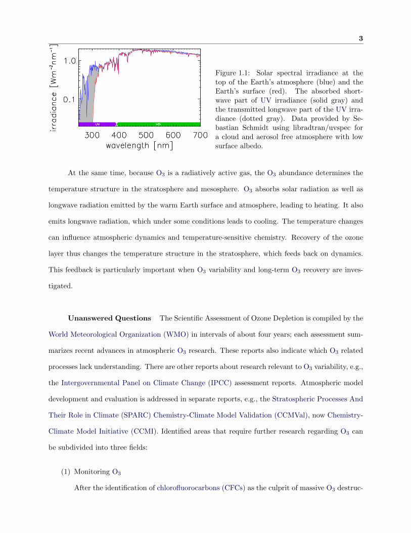
Significance The Sun is the most important energy source for the Earth’s atmosphere.
Most of this energy is transported through space by electromagnetic radiation with a spectrum
close to a Planck distribution corresponding to the solar temperature 1 . In the Earth’s atmosphere
this radiation is absorbed, reflected, and scattered by atmospheric gases and aerosols. Absorption
of electromagnetic radiation can lead to ionization and photodissociation, depending on the wave-
length of the radiation and the absorbing molecule. These processes cause particular wavelengths
to be extinguished before they reach the Earth’s surface.
Of the wavelengths reaching the Earth’s surface, the most harmful ones for life on Earth are
in the ultra violet (UV) regime and shorter since photons of that energy level can dissociate organic
molecules. For example, plants show inhibited growth, exposed human skin exhibits an erythemal
response [Leaf , 1993], and deoxyribonucleic acid (DNA) is dissociated. Reparation functions in the
skin can produce recombination errors in the DNA molecule which can result in skin cancer [Abarca
and Casiccia, 2002; van Dijk et al., 2013]. Organisms on the Earth’s surface and in the troposphere
are largely protected from this high energy radiation since molecular nitrogen (N2), molecular
oxygen (O2), and O3 are strong absorbers in the UV and shorter wavelength regime. While the
abundance of N2 and O2 throughout the atmosphere by far exceeds densities necessary to prevent
most of the harmful part of the solar radiation to reach the Earth’s surface (see Chapter 2), the
attenuation of UV wavelengths by O3 (see Figure 1.1) is more variable. This makes O3 one of the
most crucial atmospheric constituents for life on Earth. As an example, a 10% decrease in the
ozone column leads to an increase in DNA-damaging radiation at the surface of 22% [Newman,
2010].
1 The temperature referred to here is the temperature of the Sun’s photosphere which is around 5800 K.
3
Figure 1.1: Solar spectral irradiance at thetop of the Earth’s atmosphere (blue) and theEarth’s surface (red). The absorbed short-wave part of UV irradiance (solid gray) andthe transmitted longwave part of the UV irra-diance (dotted gray). Data provided by Se-bastian Schmidt using libradtran/uvspec fora cloud and aerosol free atmosphere with lowsurface albedo.
At the same time, because O3 is a radiatively active gas, the O3 abundance determines the
temperature structure in the stratosphere and mesosphere. O3 absorbs solar radiation as well as
longwave radiation emitted by the warm Earth surface and atmosphere, leading to heating. It also
emits longwave radiation, which under some conditions leads to cooling. The temperature changes
can influence atmospheric dynamics and temperature-sensitive chemistry. Recovery of the ozone
layer thus changes the temperature structure in the stratosphere, which feeds back on dynamics.
This feedback is particularly important when O3 variability and long-term O3 recovery are inves-
tigated.
Unanswered Questions The Scientific Assessment of Ozone Depletion is compiled by the
World Meteorological Organization (WMO) in intervals of about four years; each assessment sum-
marizes recent advances in atmospheric O3 research. These reports also indicate which O3 related
processes lack understanding. There are other reports about research relevant to O3 variability, e.g.,
the Intergovernmental Panel on Climate Change (IPCC) assessment reports. Atmospheric model
development and evaluation is addressed in separate reports, e.g., the Stratospheric Processes And
Their Role in Climate (SPARC) Chemistry-Climate Model Validation (CCMVal), now Chemistry-
Climate Model Initiative (CCMI). Identified areas that require further research regarding O3 can
be subdivided into three fields:
(1) Monitoring O3
After the identification of chlorofluorocarbons (CFCs) as the culprit of massive O3 destruc-
4
tion, the emission of CFCs and subsequent replacements were regulated by the Montreal
Protocol in 1987 and subsequent amendments. Questions of whether the regulations from
the Montreal Protocol and its amendments are effective [van Dijk et al., 2013, e.g.,] and
are being realized remain valid and require the close monitoring of interannual O3 varia-
tions.2 Diagnostic model simulations can evaluate our current understanding of past O3
loss seasons.
(2) Influence of climate change on O3
Estimating the long-term evolution of O3 requires consideration of climate change in ad-
dition to the decreasing anthropogenic chlorine (Cl) loading of the stratosphere. Climate
change in the stratosphere is largely due to cooling by anthropogenic carbon dioxide (CO2)
[Clough and Iacono, 1995], which substantially affects dynamics, chemistry and micro-
physics. The diagnosis of climate effects is complicated by the long time scale needed to
detect even small trends in, e.g., temperature, compared to the length of available obser-
vational records. Here models including the whole atmosphere can be used to compensate
for the insufficient observational records.
(3) Feedback of O3 recovery on climate
O3, CFCs, and CFC-replacements are radiatively active gases and thus contribute to climate
change. While O3 recovery mitigates CO2-induced cooling of the stratosphere by increased
absorption of solar shortwave radiation, O3 acts like other greenhouse gases (GHGs) in
the longwave regime. Decreases in stratospheric temperatures result in increases in the
large-scale atmospheric circulation, which masks chemical O3 loss [WMO , 2011a]. At the
same time the radiative forcing effects of the long-term reductions in CFCs and CFC-
replacements compensate for a small part of the CO2-induced cooling [WMO , 2011b]. As
for the previous point, model simulations can support observations by adding temporal and
spatial coverage of the temperature and GHG distributions.
2 One example of the ongoing monitoring effort is National Aeronautics and Space Administration (NASA)’sOzone hole watch at the Goddard Space Flight center
5
All of these three fields benefit strongly from the application of state of the art Earth System
Models (ESMs). Models represent our current understanding of atmospheric processes as well as our
ability to implement our understanding correctly. For instance, the big picture of processes affecting
stratospheric O3, explained in Chapter 2, is at least qualitatively understood [WMO , 2011a]. The
quantitative diagnosis, however, requires a precise implementation of the processes involving O3
and related species. The most significant driver behind this requirement is that climate change
occurs gradually, and thus investigations require long time series with high accuracy to draw robust
conclusions. Current model evaluation efforts (e.g., SPARC CCMI) indicate that comparisons of
stratospheric O3 simulations still show a range of results from different models [SPARC CCMVal
[2010], Figure 6.36; Charlton-Perez et al. [2010]], complicating long-term trend analyses. WMO
suggests that interactions between the middle atmosphere and the ocean are a possible source of the
variability in the results, but these interactions are currently not realized in atmospheric models.
The ultimate goal of further model development is the improvement of prognostic capabilities. In
order to gain the necessary robustness for prognostic simulations, hindcast capabilities based on
diagnostic simulations have to be improved first.
This chapter motivates the tasks model evaluation and subsequent model improvements using
diagnostic simulations. These tasks describe the first central part of this thesis. The impact of
individual processes is quantified which is the second central part of this work. Both parts are
tested for robustness by an additional case study.
Chapter 2
Polar Stratospheric Ozone
Contents
2.1 Polar Stratospheric Dynamics . . . . . . . . . . . . . . . . . . . . . . . . . . 9
2.1.1 Brewer Dobson Circulation . . . . . . . . . . . . . . . . . . . . . . . . . . 9
2.1.2 Polar Vortex . . . . . . . . . . . . . . . . . . . . . . . . . . . . . . . . . . . 11
2.1.3 Hemispheric Differences (Dynamics) . . . . . . . . . . . . . . . . . . . . 13
2.2 Polar Stratospheric Chemistry . . . . . . . . . . . . . . . . . . . . . . . . . 14
2.2.1 Photochemistry . . . . . . . . . . . . . . . . . . . . . . . . . . . . . . . . . 15
2.2.2 Gas-Phase Catalytic Chemistry . . . . . . . . . . . . . . . . . . . . . . . 17
2.2.3 Polar Stratospheric Clouds . . . . . . . . . . . . . . . . . . . . . . . . . . 23
2.2.4 Energetic Particle Precipitation . . . . . . . . . . . . . . . . . . . . . . . 27
2.2.5 Hemispheric Differences (Chemistry) . . . . . . . . . . . . . . . . . . . . 29
2.3 Investigation of Polar Stratospheric Ozone . . . . . . . . . . . . . . . . . . 29
2.4 Science Questions . . . . . . . . . . . . . . . . . . . . . . . . . . . . . . . . . 32
O3 is a molecule consisting of three oxygen atoms. The average bond order in the molecule is
1.5, which makes the O3 molecule very reactive as an oxidant. O3 has spectral absorption features
in the UV (Hartley band at 200 nm - 300 nm and Huggins band at 310 nm - 350 nm), visible (VIS)
(Chappuis band at 410 nm - 750 nm), and near infrared (NIR) (≈ 9.5µm) (see Figure 2.1). In the
atmosphere O3 appears as a trace gas with a total abundance of 7×10⁻⁶ % and highest concentra-
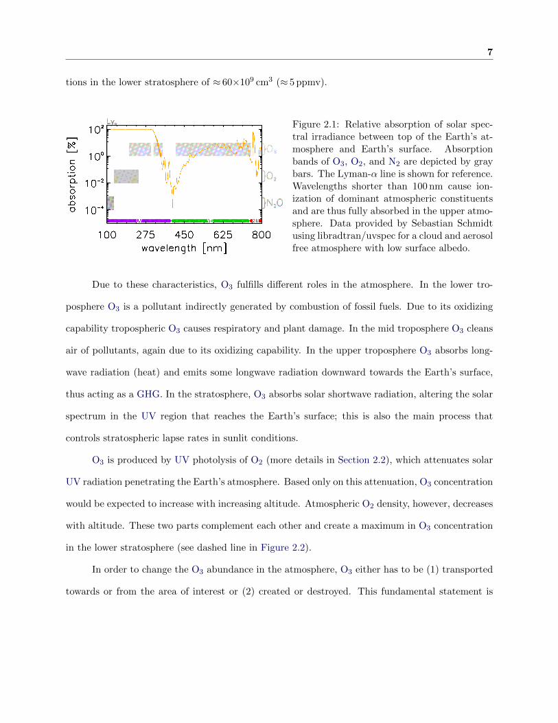
7
tions in the lower stratosphere of ≈ 60×109 cm3 (≈ 5 ppmv).
Figure 2.1: Relative absorption of solar spec-tral irradiance between top of the Earth’s at-mosphere and Earth’s surface. Absorptionbands of O3, O2, and N2 are depicted by graybars. The Lyman-α line is shown for reference.Wavelengths shorter than 100 nm cause ion-ization of dominant atmospheric constituentsand are thus fully absorbed in the upper atmo-sphere. Data provided by Sebastian Schmidtusing libradtran/uvspec for a cloud and aerosolfree atmosphere with low surface albedo.
Due to these characteristics, O3 fulfills different roles in the atmosphere. In the lower tro-
posphere O3 is a pollutant indirectly generated by combustion of fossil fuels. Due to its oxidizing
capability tropospheric O3 causes respiratory and plant damage. In the mid troposphere O3 cleans
air of pollutants, again due to its oxidizing capability. In the upper troposphere O3 absorbs long-
wave radiation (heat) and emits some longwave radiation downward towards the Earth’s surface,
thus acting as a GHG. In the stratosphere, O3 absorbs solar shortwave radiation, altering the solar
spectrum in the UV region that reaches the Earth’s surface; this is also the main process that
controls stratospheric lapse rates in sunlit conditions.
O3 is produced by UV photolysis of O2 (more details in Section 2.2), which attenuates solar
UV radiation penetrating the Earth’s atmosphere. Based only on this attenuation, O3 concentration
would be expected to increase with increasing altitude. Atmospheric O2 density, however, decreases
with altitude. These two parts complement each other and create a maximum in O3 concentration
in the lower stratosphere (see dashed line in Figure 2.2).
In order to change the O3 abundance in the atmosphere, O3 either has to be (1) transported
towards or from the area of interest or (2) created or destroyed. This fundamental statement is
8
described by the continuity equation:
d[O3]
dt=
∂[O3]
∂t+ v · ∇[O3]︸ ︷︷ ︸(1)
+ S︸︷︷︸(2)
(2.1)
where [O3] is the concentration of O3, v is the wind vector, and S represents chemical
sources and sinks of O3. The first two terms on the right (1) represent the transport of O3,
which is controlled by atmospheric dynamics (see Section 2.1). The third term on the right (2)
represents the creation or destruction of O3 (source/sink), which is controlled by atmospheric
chemistry (see Section 2.2). When investigating and quantifying O3 loss the distinction between
these two contributors to O3 change is crucial since they can mimic or mask each other. At the same
time, observations of O3 can only provide the total change in O3 with time, e.g., comparing the two
curves in Figure 2.2. The distinction between dynamics and chemistry requires either observations
that are taken by in-situ Lagrangian instruments (e.g., balloons) or meteorological observations of
transport parameters (e.g., winds). This challenge must be addressed by any study investigating
atmospheric O3 loss; the approach taken here is explained in Chapter 3 [Brakebusch et al., 2013].
The dramatic decrease of the O3 layer shown in Figure 2.2 is known as the O3 hole and
occurs during spring time in the polar regions. The O3 hole is defined as the area in which the total
column abundance of O3 is less than 220 Dobson Units (DU). In order to understand the formation,
evolution, hemispheric differences, interannual variability, and impact of severe O3 loss events, all
involved processes must be explained. As described before, these processes can be categorized
as dynamical and chemical processes. In the next two sections the relevant polar stratospheric
dynamical mechanisms are characterized, followed by a description of the most important polar
stratospheric chemical processes. This chapter then concludes with a compilation of requirements
for investigating polar stratospheric O3 and, based on that, develops remaining science questions
that are answered in the subsequent chapters.

2.1. Polar Stratospheric Dynamics 9
Figure 2.2: ”Vertical distribution of the ozonepartial pressure (nbar) observed at Halley BayStation on August 15, 1987 (high values), andOctober 15, 1987 (low values), respectively.(Farman, personal communication, 1987)”.1
2.1 Polar Stratospheric Dynamics
As described in Chapter 2, O3 abundances are in part controlled by transport. Thus at-
mospheric dynamics are essential to explain the distribution of O3. In the following paragraphs
the main dynamical features affecting O3 in the winter polar region, the Brewer Dobson circu-
lation (BDC) and the polar vortex, are described; the section concludes with an explanation of
hemispheric differences.
2.1.1 Brewer Dobson Circulation
Strongest O3 production occurs in the equatorial stratosphere due to maximized solar insola-
tion, while highest O3 abundances are observed in the polar lower stratosphere [WMO , 2003]. This
1 Reproduced from WMO (World Meteorological Organization) (1990), Report of the International Ozone TrendsPanel: 1988, Global Ozone Research and Monitoring Project, Report No. 18.
2.1. Polar Stratospheric Dynamics 10
apparent contradiction was first explained by Brewer [1949] and Dobson [1956], who proposed a
tropical convective motion into the stratosphere followed by advection towards the winter pole and
subsequent adiabatic descent at high latitudes. This circulation pattern is known as the BDC. The
meridional gradient in solar insolation caused by the difference in mean solar zenith angle (SZA) be-
tween the equator and the winter polar region results in a meridional temperature gradient near the
Earth’s surface and thus a meridional pressure gradient. This pressure gradient creates a meridional
tropospheric wind that is deflected by the Coriolis force. Once geostrophic balance is established,
this wind is purely westerly at about mid-latitudes. Flow over large topographic features stretches
and compresses the vertical extent of the flow (a thermal forcing due to land-sea contrast is also
possible). In order to preserve potential vorticity (PV) this deformation is balanced by a change
in relative vorticity, which results in a horizontally oscillating planetary wave (PW) also called a
Rossby wave. Charney and Drazin [1961] showed that PWs have an easterly phase velocity and
that they can propagate upward only if the background mean wind speed is westerly. While on
average this background mean wind in the troposphere is westerly the entire year, the stratospheric
mean winds change direction semiannually [Reed , 1966]. In the stratosphere the summer pole is
heated due to solar UV absorption by O3 while the winter pole is radiatively cooled, resulting in
a temperature gradient spanning both hemispheres. Thus the geostrophic balance creates an east-
erly flow in the stratospheric summer hemisphere and a westerly flow in the stratospheric winter
hemisphere, called the stratospheric polar night jet (PNJ). Thus PWs cannot propagate into the
stratosphere in the summer hemisphere. Charney and Drazin [1961] also showed that even if the
stratospheric winds are westerly, the phase speed of the PW must not exceed a critical value in
order to allow upward propagation. This critical wind speed depends on the wavelength of the PW,
effectively filtering higher wavenumbers. In fact only PWs with wavenumbers 1-3 are observed in
the stratosphere. A stable PW is only maintained when non-linear components can be neglected.
Since the amplitude of PWs increases with altitude, non-linear effects2 increase in magnitude as
2 Conservation of PV is given when the wave motion can be described with the quasi-geostrophic PV equation whichis a linearized equation [Holton, 2004]. When PV is conserved, any deformation of material contours is reversible.If the amplitude becomes larger, non-linear terms are not negligible anymore and the flow cannot be approximated
2.1. Polar Stratospheric Dynamics 11
well and the PW becomes unstable [Holton, 2004]. When the PW breaks its easterly phase speed
results in an easterly momentum deposition, which slows or even reverses the zonal mean flow.
Since the meridional component of the Coriolis force is proportional to the zonal wind speed, a
poleward motion is induced when the geostrophic balance is reestablished. The breaking of PWs
thus results in a net poleward movement, which is the driver of the BDC. This convergence of air
masses in the polar region causes downward transport to preserve mass continuity. Downward mo-
tion then subsequently leads to adiabatic compression, thereby heating the winter stratosphere to
temperatures above the radiative equilibrium temperature calculated by diabatic radiative cooling
alone.
2.1.2 Polar Vortex
The stratospheric PNJ forms a strong cyclone that is present in the stratosphere and some-
times extends into the mesosphere. This cyclone is commonly referred to as the polar vortex. The
distinct feature of the polar vortex is that it represents a barrier to horizontal transport. It can
be shown that under the assumption of horizontal transport being purely adiabatic and the PNJ
being purely geostrophic that PV is conserved for air parcels in the PNJ and that the meridional
gradient of PV is very steep across the PNJ [e.g., Brasseur and Solomon, 2005]. Thus PV is a
restoring force for air parcels in the PNJ while it has a repulsive effect on air parcels with higher
or lower PV. For practical purposes a PV threshold can be used to define the edge of the polar
vortex. When the previously discussed PWs break due to the PNJ, they deposit westward angular
momentum, which slows the zonal wind speed of the PNJ. In order to conserve PV of the flow,
the PNJ is deformed and locally gains meridional wind components [e.g., Shepherd , 2000]. The
net poleward motion described in Section 2.1.1 causes increased descent after breaking PWs due
to mass conservation. This increased descent leads to adiabatic warming; such events are called
sudden stratospheric warming (SSW)s [Matsuno, 1971]. These warmings are classified into three
with the quasi-geostrophic PV equation. In that case PV is not conserved which results into irreversible deformationof material contours, also called wave-breaking.

2.1. Polar Stratospheric Dynamics 12
categories: (1) minor warming3 , (2) major warming4 , and (3) final warming5 [McInturff , 1978;
Andrews et al., 1987]. Observations show that the polar vortex is deformed and displaced from
the pole when PWs with wavenumber 1 break and the vortex is split into two cyclones when PWs
with wavenumber 2 break [Shepherd , 2000]. The disturbance of PV due to wave breaking is usually
accompanied by horizontal mixing or intrusion and extrusion of filaments. If the PW-breaking is
too strong for the weak late season westerly PNJ, the winds are permanently reversed until the
next winter season and air masses inside and outside the polar vortex are not isolated from each
other anymore. This PW-breaking event is called final warming. In addition to the large-scale
PWs that oscillate in a horizontal plane due to the restoring Coriolis force, another type of wave
exists that oscillates in a vertical plane due to gravity as the restoring force. Hence these waves are
called gravity wave (GW)s. Similar to PWs, the initial creation of GWs can be due to tropospheric
flow over topography; but other sharp boundaries such as convection or frontal processes give rise
to GWs as well [Fritts and Alexander , 2003]. GWs can have phase speeds that are westward or
eastward and their wavelength of 10 km - 1000 km is much shorter than that of PWs. Also they
are more frequent but carry less energy than PWs. The polar, upward propagation of GWs is also
affected by the PNJ, which filters GWs that have phase speeds that are slower than but in the same
direction as the PNJ [Andrews et al., 1987]. Deposition of angular momentum from filtered GWs
into the PNJ is small compared to PW breaking and can cause not more than a small amount of
mixing across the polar vortex edge. Aside from the filtering, the reason for GW-breaking is their
growth in amplitude as they propagate vertically. At a critical level the amplitude becomes too
large to be convectively stable; this usually occurs in the mesosphere. Breaking GWs in the meso-
sphere are connected to descent in the upper atmosphere [Andrews et al., 1987] and thus become
important for the stratosphere due to transport of, e.g., reactive nitrogen species generated in the
upper atmosphere by energetic particle precipitation (EPP) (see Section 2.2.4).
3 Minor warmings are defined as a reversal of the zonal mean temperature gradient without a reversal of the zonalmean zonal wind to easterly direction.
4 Major warmings are defined as a zonal mean temperature increase at ≥10 hPa poleward from 60◦ latitude andreversal of the zonal mean zonal wind to easterly.
5 The final warming is defined as a reversal of the mean zonal wind to easterly direction without recovery.
2.1. Polar Stratospheric Dynamics 13
2.1.3 Hemispheric Differences (Dynamics)
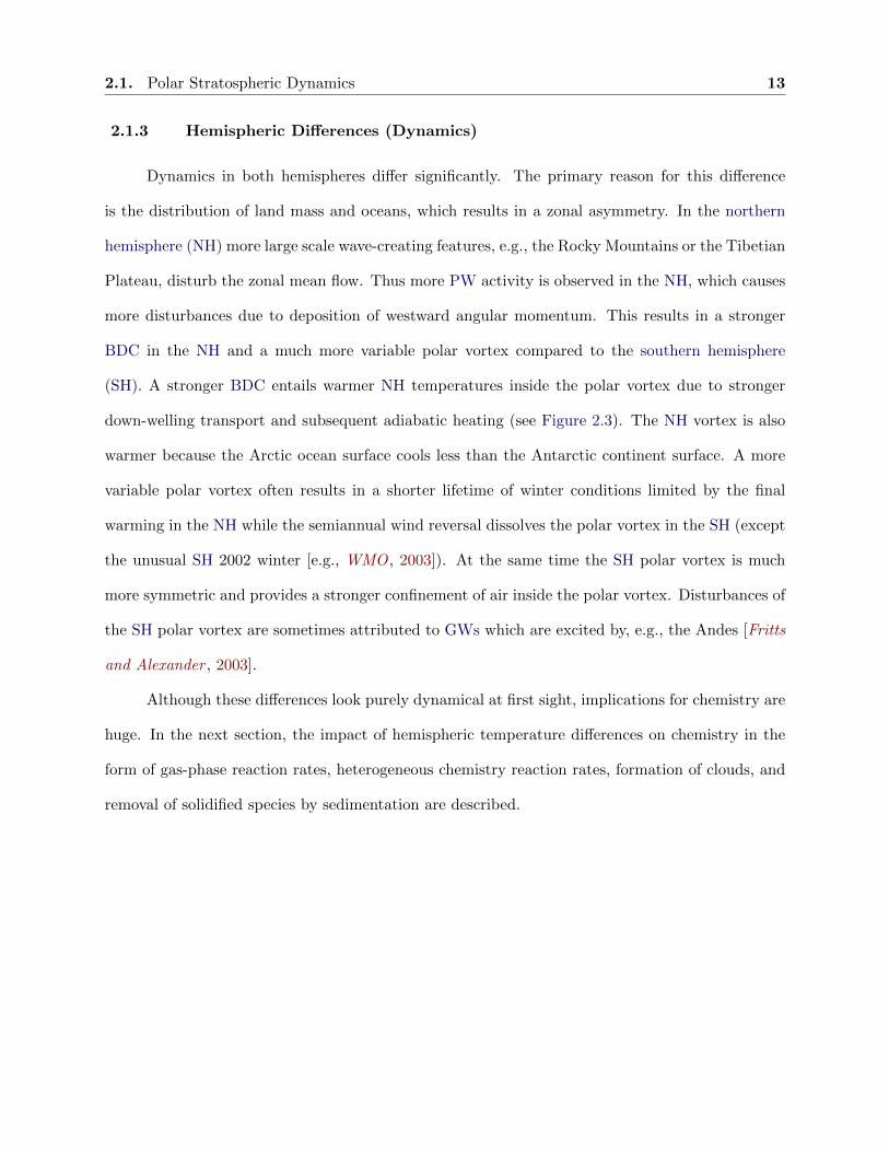
Dynamics in both hemispheres differ significantly. The primary reason for this difference
is the distribution of land mass and oceans, which results in a zonal asymmetry. In the northern
hemisphere (NH) more large scale wave-creating features, e.g., the Rocky Mountains or the Tibetian
Plateau, disturb the zonal mean flow. Thus more PW activity is observed in the NH, which causes
more disturbances due to deposition of westward angular momentum. This results in a stronger
BDC in the NH and a much more variable polar vortex compared to the southern hemisphere
(SH). A stronger BDC entails warmer NH temperatures inside the polar vortex due to stronger
down-welling transport and subsequent adiabatic heating (see Figure 2.3). The NH vortex is also
warmer because the Arctic ocean surface cools less than the Antarctic continent surface. A more
variable polar vortex often results in a shorter lifetime of winter conditions limited by the final
warming in the NH while the semiannual wind reversal dissolves the polar vortex in the SH (except
the unusual SH 2002 winter [e.g., WMO , 2003]). At the same time the SH polar vortex is much
more symmetric and provides a stronger confinement of air inside the polar vortex. Disturbances of
the SH polar vortex are sometimes attributed to GWs which are excited by, e.g., the Andes [Fritts
and Alexander , 2003].
Although these differences look purely dynamical at first sight, implications for chemistry are
huge. In the next section, the impact of hemispheric temperature differences on chemistry in the
form of gas-phase reaction rates, heterogeneous chemistry reaction rates, formation of clouds, and
removal of solidified species by sedimentation are described.

2.2. Polar Stratospheric Chemistry 14
Figure 2.3: Evolution of minimum temperature in the polar stratosphere. While the Arctic tem-peratures are warmer, also the variability in the Arctic is larger than in the Antarctic.6
2.2 Polar Stratospheric Chemistry
Sources and sinks of O3 in the Earth’s atmosphere are determined by photochemistry (Sec-
tion 2.2.1) and gas-phase chemistry (Section 2.2.2). The latter is in part preceded by heterogeneous
chemistry (Section 2.2.3) that mostly occurs on polar stratospheric cloud (PSC) surfaces in low-
temperature polar winter conditions. In this section, all of these types of chemistry are explained.
EPP, which is a highly variable source of reactive nitrogen oxide (NOX), is introduced as well
(Section 2.2.4). This section concludes with the description of hemispheric differences in polar
stratospheric chemistry (Section 2.2.5).
6 Reproduced from WMO (World Meteorological Organization) (2011), Twenty Questions and Answers Aboutthe Ozone Layer: 2010 Update, D. W. Fahey and Hegglin, M. I. (Coordinating Lead Authors), Scientific Assessmentof Ozone Depletion: 2010.

2.2. Polar Stratospheric Chemistry 15
2.2.1 Photochemistry
The formation of O3 is preceded by the photolysis of O2, which forms atomic oxygen (O)
(Reaction 2.2). In an exothermal three body reaction O and O2 then combine to form O3 (Reac-
tion 2.3). Because fast photolysis of O3 also forms O (Reaction 2.4), O and O3 are interchanged
rapidly. Also, O and O3 can recombine (Reaction 2.5) to form O2.
O2 + hνJO2−→ O + O [λ ≤ 242.4nm] (2.2)
O + O2 + MkO2−→ O3 + M [exothermal] (2.3)
O3 + hνJO3−→ O2 + O [200nm ≤ λ ≤ 350nm] (2.4)
O + O3
kO3−→ O2 + O2 (2.5)
Here, the letters J and k are the reaction rate constants and M represents a third body nec-
essary for momentum and energy deposition; thus M can be any atmospheric constituent. Strato-
spheric reactions requiring a third body depend highly on atmospheric density, making them more
likely in the lower stratosphere. Because of the rapid interchange between O3 and O, they are often
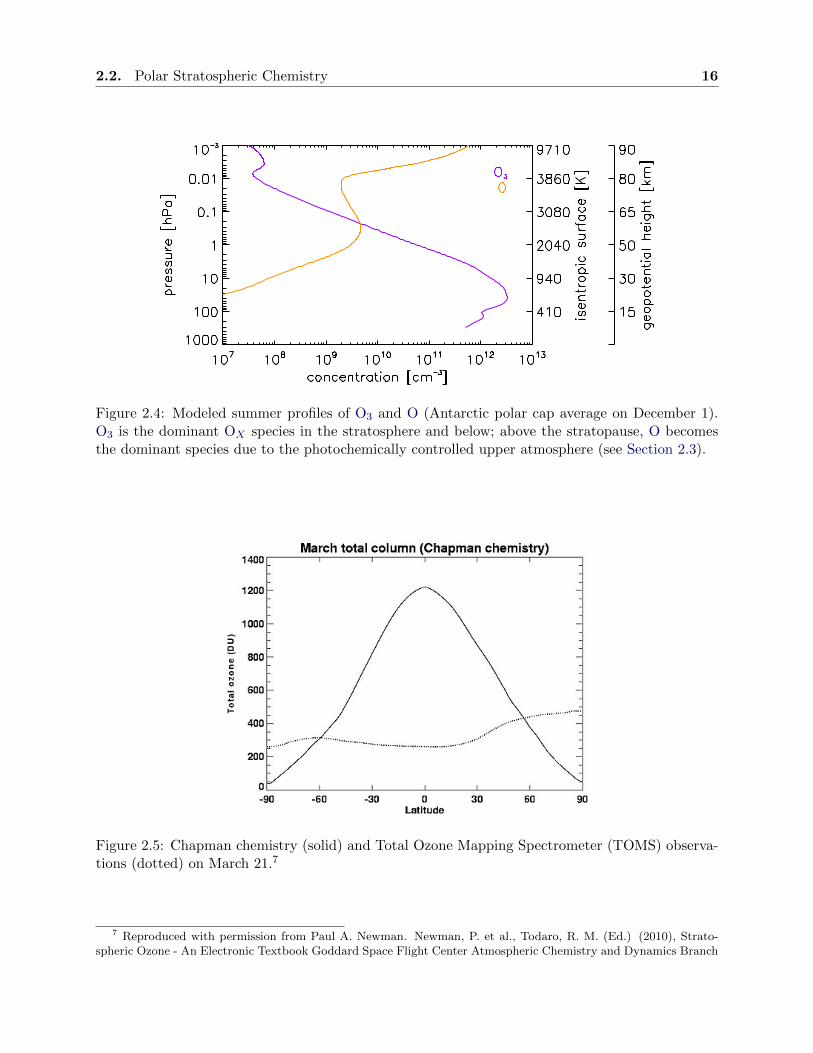
treated together as the odd oxygen (OX) family (Figure 2.4).
Note that Reaction 2.3 and Reaction 2.4 do not change the concentration of OX ([Ox]) but
have to be considered nevertheless since reaction Reaction 2.5 equally depends on O and O3. Thus
the source term in the continuity equation is given as
∂[Ox]
∂t= 2JO2 [O2]−
2kO3JO3 [O3]2
kO2M[O2]. (2.6)
The OX chemistry described above was found by Chapman [1930] and it applies to a sta-
tionary atmosphere with oxygen-only chemistry. Global observations show, however, that column
densities of equatorial O3 are overestimated and O3 in the polar region is underestimated, if only
Chapman chemistry is considered (see Figure 2.5). Gas-phase catalytic chemistry as well as the
BDC must be taken into account in order to describe the real O3 distribution.
2.2. Polar Stratospheric Chemistry 16
Figure 2.4: Modeled summer profiles of O3 and O (Antarctic polar cap average on December 1).O3 is the dominant OX species in the stratosphere and below; above the stratopause, O becomesthe dominant species due to the photochemically controlled upper atmosphere (see Section 2.3).
Figure 2.5: Chapman chemistry (solid) and Total Ozone Mapping Spectrometer (TOMS) observa-tions (dotted) on March 21.7
7 Reproduced with permission from Paul A. Newman. Newman, P. et al., Todaro, R. M. (Ed.) (2010), Strato-spheric Ozone - An Electronic Textbook Goddard Space Flight Center Atmospheric Chemistry and Dynamics Branch

2.2. Polar Stratospheric Chemistry 17
2.2.2 Gas-Phase Catalytic Chemistry
In addition to Chapman’s pure-oxygen chemistry described above, the equilibrium amount
of O3 is controlled by catalytic reactions with a catalyst X according to the general scheme:
O3 + X −→ XO + O2 (2.7)
XO + O −→ X + O2 (2.8)
net : O3 + O −→ 2O2. (2.9)
Species that can most efficiently fulfill the role of catalyst X are hydroxyl radical (OH), nitro-
gen oxide (NO), and inorganic halogens. The following section summarizes gas-phase destruction
of O3 for these catalysts, their atmospheric abundance and relevance. The section will conclude
with coupling reactions between catalysts.
Reactive Odd Hydrogen The O3 chemistry related to odd hydrogen (HOX), which
consists of atomic hydrogen (H), OH, and peroxyl radical (HO2), was first investigated by Bates
and Nicolet [1950]. The dominant sources of polar HOX in the middle and upper stratosphere are
the oxidation of water vapor (H2O) and methane (CH4) transported from the tropical troposphere
via the BDC:
OH + CH4 −→ H2O + CH3 (2.10)
H2O + O(1D) −→ 2OH. (2.11)
Since the second step requires singlet D oxygen (O(1D)), OH is primarily formed in the upper
stratosphere where OX is dominated by O(1D) due to UV photolysis. This dependence on UV
radiation also causes a strong diurnal variation, with HOX abundances being highest around local
noon. Although H2O is abundant in the troposphere, transport of H2O from the the troposphere
into the stratosphere is limited because of the low tropopause temperature [Kley et al., 1982;
(Code 916).
2.2. Polar Stratospheric Chemistry 18
Jackson et al., 1998; Salby et al., 2003]. HOX is also created sporadically in the stratosphere by
precipitating solar protons or relativistic electrons (see Section 2.2.4). Additional anthropogenic
sources of OX in the stratosphere are indirectly present in the form of additional CH4 production
by livestock farming and growing swamps caused by melting of tundra regions. The sink for
HOX in the stratosphere is the sedimentation of the reservoir species H2O, nitric acid (HNO3),
and peroxynitric acid (HNO4). Depending on altitude several catalytic O3 destruction cycles are
possible. In the upper stratosphere the following two cycles are possible due to the abundance of
O:
OH + O3 −→ HO2 + O2 (2.12)
HO2 + O −→ OH + O2 (2.13)
net : O3 + O −→ 2O2, (2.14)
H + O2 + M −→ HO2 + M (2.15)
HO2 + O −→ OH + O2 (2.16)
OH + O −→ H + O2 (2.17)
net : 2O −→ O2. (2.18)
The following cycle is possible throughout the stratosphere:
OH + O3 −→ HO2 + O2 (2.19)
HO2 + O3 −→ OH + 2O2 (2.20)
net : 2O3 −→ 3O2. (2.21)
Since the lifetime of HOX is short compared to other catalysts that destroy O3, the relevance
for long-term O3 loss is low [Brasseur and Solomon, 2005]. However, because of the short lifetime,

2.2. Polar Stratospheric Chemistry 19
HOX is a good indicator of energetic particle precipitation into the stratosphere, since this creates
a transient increase in HOX (see Section 2.2.4).
Reactive Odd Nitrogen Crutzen [1970] found that NOX , which consists of NO and NO2
in the stratosphere, has a significant impact on O3 destruction. NOX in the stratosphere originates
primarily from nitrous oxide (N2O) via the following reactions:
N2O + hν −→ NO + N(4S) [λ ≤ 200 nm] (2.22)
N(4S) + O2 −→ NO + O (2.23)
N2O + O(1D) −→ 2NO. (2.24)
The stratospheric source of N2O is transport from the troposphere via the BDC, where N2O
naturally comes from soils in the tropical forest and the oceans. This source is anthropogenically
enhanced by soil cultivation using common fertilizers and biomass burning [WMO , 1995]. Since
the production of NOX from N2O depends on UV radiation and the abundance of O(1D), NOX is
primarily created in the upper stratosphere. Another stratospheric NOX source is NOX produced in
the mesosphere by EPP that subsequently descends into the polar stratosphere (see Section 2.2.4).
The primary O3 destruction due to NOX is described by the following catalytic cycle
NO + O3 −→ NO2 + O2 (2.25)
NO2 + O −→ NO + O2 (2.26)
net : O3 + O −→ 2O2. (2.27)
Many chemical reactions compete with this cycle, notably the deposition of NOX into the
night time reservoir nitrogen pentoxide (N2O5) via
NO2 + O3 −→ NO3 + O2 (2.28)
NO3 + NO2 + M −→ N2O5 + M, (2.29)
2.2. Polar Stratospheric Chemistry 20
and the release from the reservoir via
N2O5 + hν −→ NO3 + NO2 [λ ≤ 380 nm] (2.30)
NO3 + hν −→ NO2 + O [λ ≤ 620 nm]. (2.31)
The above reactions result in a strong diurnal variation of the nitrogen partitioning. NOX also
interferes with other O3 destroying catalysts, typically forming reservoir species like peroxinitric
acid (HO2NO2), HNO3, chlorine nirate (ClONO2), and bromine nirate (BrONO2). If NOX is
incorporated into the HNO3 reservoir, it can permanently be removed from the stratosphere. This
occurs via the formation of HNO3-containing PSCs, followed by sedimentation of the PSCs (see
Section 2.2.3). The formation of PSCs, however, can amplify chlorine chemistry (see Section 2.2.3).
Thus nitrogen species, summarized as total reactive odd nitrogen (NOY ), fulfill several roles in
the picture of polar stratospheric O3 loss both destroying O3 and reducing O3 loss by forming the
ClONO2 reservoir which effectively reduces total reactive chlorine (ClOX) (see Section 2.2.3).
Inorganic Halogens Although the list of primordial halogens includes fluorine (F), Cl,
bromine (Br), and iodine (I), only Cl and Br are of importance for stratospheric O3 loss. This is
due to the rapid irreversible formation of hydrogen fluoride (HF), which does not participate in O3
chemistry [Stolarski and Rundel , 1975]. I is more efficient in destroying O3 than Cl and Br due to a
higher fraction of I being in reactive forms; but nevertheless the I abundance in the stratosphere is
negligible [Wennberg et al., 1997; Pundt et al., 1998; Cox et al., 1999]. Since Cl and Br participate
in very similar chemical reactions [e.g., Yung et al., 1980; Poulet et al., 1992] both are summarized
in this section. A natural source of halogens in the stratosphere is the convection of the insoluble
methyl chloride (CH3Cl) and methyl bromide (CH3Br), which are photolyzed in the upper strato-
sphere. The halogen abundance, however, is dramatically altered by the vast use of CFCs. These
stable molecules were invented in the late 19th century and have no natural occurrence. Around
1928 CFCs were recognized as non-toxic and non-reactive replacements for refrigerants, solvents,
aerosol propellants, and fire retardants [e.g., Sneader , 2005]. Shortly after, CFCs were produced

2.2. Polar Stratospheric Chemistry 21
on commercial scales and after about 1960 their atmospheric abundance increased dramatically
[Lovelock , 1971; Walker et al., 2000]. Once CFCs are transported to the upper stratosphere they
are photolyzed, producing Cl and Br radicals. Thus the halogen abundance in the stratosphere was
increased by ≈ 500 % of the natural abundance by the mid-1990s. Molina and Rowland [1974] as
well as Stolarski and Cicerone [1974] investigated the dramatic O3 destruction potential of CFCs.
After Farman et al. [1985] reported dramatic decreases in Antarctic O3 due to chlorine chemistry
(see Figure 2.2), CFCs were soon confirmed as the primary source of polar stratospheric Cl leading
to the substantial O3 loss. In an unprecedented international collaboration the Montreal Protocol
was signed in 1987 regulating the phase-out of CFCs; subsequent amendments regulate the phase-
out of the less harmful immediate replacements. Nowadays, substances like R-410A8 are used as
refrigerants that have no O3 depletion potential. Molina and Rowland [1974] proposed that the
following catalytic cycle is responsible for Cl-induced catalytic O3 destruction:
Cl + O3 −→ ClO + O2 (2.32)
ClO + O −→ Cl + O2 (2.33)
net : O3 + O −→ 2O2. (2.34)
Since this cycle requires the abundance of O it can only happen in the upper stratosphere and
thus cannot sufficiently explain the O3 loss observed. Accordingly, Molina and Molina [1987] pro-
posed the termolecular self-reaction of chlorine monoxide (ClO) to replace Reaction 2.33, followed
by photolysis and further reaction of the products:
2ClO + M −→ ClOOCl + M (2.35)
ClOOCl + hν −→ ClOO + Cl [200 nm ≤ λ ≤ 420 nm] (2.36)
ClOO + M −→ Cl + O2 + M. (2.37)
8 R-410A is a difluoromethane (CH2F2) and pentafluoroethane (CHF2CF3) mix.
2.2. Polar Stratospheric Chemistry 22
Note that this cycle does not require O, and thus considering this cycle increases reaction
rates for Cl-induced O3 loss in the lower stratosphere. Also McElroy et al. [1986] and Tung et al.
[1986] proposed a Cl/Br coupled reaction scheme to replace Reaction 2.33:
ClO + BrO −→ BrCl + O2 (2.38)
BrCl + hν −→ Br + Cl. (2.39)
The cycles here strongly depend on ClO and bromine monoxide (BrO) abundances and can
only explain the observed O3 depletion if the release of Cl and Br from the reservoir species
hydrogen chloride (HCl), ClONO2, hydrogen bromide (HBr), and BrONO2 does not occur by
photolysis alone. This finding marked the onset of research investigating the activation of Cl and
Br via heterogeneous chemistry on PSC surfaces during polar night [Crutzen and Arnold , 1986;
McElroy et al., 1986; Solomon et al., 1986].
Gas-Phase Coupling Reactions The catalysts and corresponding reservoir species par-
ticipate in chemical reactions that couple HOX , NOX , ClOX and reactive bromine (BrOX) species.
Aside from the ClO/BrO cycle (Reaction 2.38 and Reaction 2.39) presented in the previous para-
graph, those coupling reactions often hamper the O3 loss cycles and/or result in production of
reservoir species. For instance, essential coupling reactions between ClOX and NOX are
ClO + NO −→ Cl + NO2 (2.40)
ClO + NO2 + M −→ ClONO2 + M (2.41)
ClONO2 + hν −→ Cl + NO3 (2.42)
NO3 + hν −→ NO2 + O. (2.43)
While the Reaction 2.40 is beneficial for the Cl-induced O3 loss cycle by reforming Cl without
requiring O, it reduces the reaction rate of NO-induced O3 loss (Reaction 2.25). Reaction 2.41 slows
both Cl-induced and NO-induced O3 loss by forming the reservoir ClONO2. Since ClONO2 needs to
2.2. Polar Stratospheric Chemistry 23
be photolyzed (Reaction 2.42) in order to provide Cl and nitrogen dioxide (NO2) (after subsequent
photolysis of nitrate radical (NO3)), O3 loss is slowed down during night time periods.
This section illustrates that the three major catalysts Cl, Br, and NO cannot be considered
separately from each other. Thus it is pointed out that in order to understand O3 loss cycles all
processes have to be considered simultaneously. In particular, the simultaneous presence of NOX
and ClOX results in formation of the ClONO2 reservoir, reducing the lifetime and abundance of
ClOX and NOX , and thus hampering O3 destruction cycles.
2.2.3 Polar Stratospheric Clouds
In Section 2.2.2, heterogeneous chemistry on PSC surfaces was pointed out as a crucial process
for activation of halogens from their reservoir species. Counter-intuitively, low abundances of NO2
before and during O3 loss periods were observed [Noxon et al., 1978; Fahey et al., 1989] when PSCs
were present. Condensation nuclei for PSCs originate from sulfate emission in the troposphere.
Dominant natural sources are the oceans, volcanic eruptions, and biomass burning [Bates et al.,
1992]. These sources are by far exceeded by anthropogenic sources primarily due to the combustion
of coal. Although most of the sulfates are removed in the troposphere via dry and wet deposition
[Brasseur and Solomon, 2005], they can reach the tropical stratosphere in the form of the stable
carbonyl sulfide (COS) molecule [Crutzen, 1976]. Volcanic eruptions are capable of direct sulfur (S)
deposition into the stratosphere and thus represent a sporadic source of stratospheric COS [IPCC ,
2007]. In the stratosphere COS gets photolyzed and ultimately forms sulfuric acid (H2SO4) via the
chain:

2.2. Polar Stratospheric Chemistry 24
COS + hν −→ CO + S (2.44)
S + O2 −→ SO + O (2.45)
SO + O2 −→ SO2 + O (2.46)
SO2 + OH + M −→ HSO3 + M (2.47)
HSO3 + O2 −→ HO2 + SO3 (2.48)
SO3 + H2O −→ H2SO4. (2.49)
Of the species in this chain, sulfur monoxide (SO), hydrogen sulfite (HSO−3 ), and H2SO4
are soluble in ambient H2O and form sulfate aerosols that provide surface area density (SAD) for
heterogeneous chemistry. Sinks for stratospheric sulfate aerosols (SSAs) are downwelling transport
and sedimentation with subsequent wet deposition [Turco et al., 1982]. SSAs with radii greater
than 0.1µm accumulate several kilometers above the tropopause, forming the stratospheric aerosol
layer [Junge et al., 1961; Junge and Manson, 1961].
The saturation vapor pressure for ambient H2O decreases when stratospheric temperature
declines during the polar night. Thus SSAs take up more H2O by condensational growth, forming
a binary solution of H2SO4/H2O. At temperatures below ≈200 K all H2SO4 is assumed to be part
of this binary solution. Since the H2O uptake continues below ≈200 K the mass fraction of H2SO4
decreases.
At temperatures from≈193 K to≈191 K the saturation vapor pressure for HNO3 is sufficiently
low that the binary aerosol particles described previously gradually change to a binary composition
of H2SO4/HNO3/H2O, with the H2SO4 fraction becoming very small. In this transition region
particles are called supercooled ternary solution (STS) [Lowe and MacKenzie, 2008]. The STS
particles (or Type Ib) are liquid, have typical radii of 0.5µm, and are too small to sediment [Toon
et al., 1990]. In addition to providing SAD via uptake of HNO3, STS particles also take up gas-
phase HCl and HBr, making them unavailable for halogen activation [Carslaw et al., 1995]. The
temperature regime in which STS particles exist occurs regularly in average and cold Arctic winters

2.2. Polar Stratospheric Chemistry 25
and thus STS particles are the dominant source of SAD in the NH.
In addition to liquid PSC particles, solid particles containing HNO3 are also important for
O3 loss. The temperature threshold for the formation of these solid PSC particles is as high as
≈195 K in the lower stratosphere [Hanson and Mauersberger , 1988]. Observations show, however,
that in addition to low temperatures, supersaturation is needed for these particles to nucleate [Dye
et al., 1990, 1992]. These particles consist of nitric acid trihydrate (NAT) or Type Ia) [e.g., Fahey
et al., 1989; Toon et al., 1990; Voigt et al., 2000]. Although NAT particle radii are typically between
1µm and 5µm, particles with larger radii of 10µm to 20µm also exist [Fahey et al., 2001]. Large
particles can sediment out of the stratosphere, with rates on the order of 60 m/h for particles with
radii of 14µm, removing HNO3 in a process known as denitrification [e.g., Toon et al., 1986]. This
occurs more often in the SH due to hemispheric temperature differences (see Section 2.1.3 and
Section 2.2.5).
The second type of solid PSC particles, which is primarily made of ice, is formed when the
temperature drops below ≈188 K. These ice particles were proposed by Steele et al. [1983] and
confirmed with observations by Poole and McCormick [1988] and Fahey et al. [1990] for the SH
and by Carslaw et al. [1998a,b] for the NH. Ice particles are also known as Type II. Radii of ice
particles range from ≈1µm to 30µm; sedimentation rates are about 100 m/h for a particle radius
of 20µm [e.g., Brasseur and Solomon, 2005]. The sedimentation causes dehydration of the lower
stratosphere [Kelly et al., 1989] and appears commonly in the SH, but is very unusual for the NH
due to higher temperatures there.
The magnitude of O3 loss can only be explained when Cl from both reservoir species HCl
and ClONO2 is made available in reactive form. Gas-phase reactions and O2 photolysis alone
cannot reproduce observed O3 loss during polar night conditions. Solomon et al. [1986] proposed
heterogeneous chemistry reactions on the surface of PSCs that produce molecular chlorine (Cl2)
and suppress the formation of NO2 [Toon et al., 1986]:
ClONO2 + HCl −→ HNO3 + Cl2 (2.50)

2.2. Polar Stratospheric Chemistry 26
Subsequent photolysis of Cl2 produces Cl which participates in O3 destruction reactions.
Over time more heterogeneous reactions on PSC surfaces were confirmed [Solomon, 1999, and
references therein]:
N2O5 + H2O −→ 2HNO3 (2.51)
ClONO2 + H2O −→ HNO3 + HOCl (2.52)
HCl + HOCl −→ H2O + Cl2 (2.53)
BrONO2 + HCl −→ HNO3 + BrCl (2.54)
BrONO2 + H2O −→ HNO3 + HOBr (2.55)
HCl + HOBr −→ H2O + BrCl. (2.56)
Note that these reactions do not produce ClOX directly but require subsequent photolysis
of Cl2 or bromine chloride (BrCl). Also, all NOY produced is in the form of stable HNO3, thus
concentrations of ClONO2 and BrONO2 are substantially reduced. In summary, PSCs play two
essential roles in large scale polar stratospheric O3 destruction: they provide SAD for heterogeneous
chemistry and at the same time denitrify and dehydrate the atmosphere as described earlier.
Heterogeneous chemistry is extremely sensitive to small temperature variations. This is re-
flected by the strong dependence of the uptake coefficient on temperature [Carslaw et al., 1997].
This causes even small temperature changes to result in dramatic changes in heterogeneous chem-
istry reaction rate coefficients. The uptake coefficient γ is defined as the ratio of the number of
collisions on a surface that lead to a reaction to the total number of collisions on a surface; thus the
uptake coefficient represents a reaction probability which can also be expressed in values between
0 % and 100 %. Figure 2.6 shows the temperature dependence of uptake coefficients for the major
heterogeneous reactions ClONO2 + HCl (Reaction 2.50), ClONO2 + H2O (Reaction 2.52), and
HCl + hypochlorous acid (HOCl) (Reaction 2.53) on STS particles [Lowe and MacKenzie, 2008].
Figure 2.6 illustrates that the reaction probability of the dominant ClONO2 + HCl reac-
tion (2.50) on STS increases from ≈ 0.1 % at 200 K to ≈ 100 % at 192 K. The resulting rate for

2.2. Polar Stratospheric Chemistry 27
heterogeneous production of Cl2 is described as
d[Cl2]
dt=v
4[ClONO2][HCl]SAD(T)γ(T ) (2.57)
with v describing the mean molecular velocity [e.g., Moore, 1962]. For typical lower strato-
spheric conditions Reaction 2.50 leads to a change in reaction rate from 2 × 10⁻⁷ mol/s at 198 K
to 1 × 10⁻³ mol/s at 190 K [e.g., Wegner , 2012]. This example illustrates that for investigations
of heterogeneous chemistry in the lower stratosphere the accurate knowledge of temperature is a
crucial requirement.
Figure 2.6: ”Reactive uptake coefficients asa function of temperature for heterogeneousreactions occurring in liquid sulphuric acidaerosols. Reaction ClONO2 + H2O is repre-sented by the green line, ClONO2 + HCl bythe blue line, and HOCl + HCl by the redline. The uptake coefficients are calculated us-ing the parameterization of Shi et al. [2001],which takes into account the couplings of thesereactions.”9
2.2.4 Energetic Particle Precipitation
While the dominant source of NOX in the stratosphere is the oxidation of N2O (see Sec-
tion 2.2.2), EPP represents an additional source of NOX . Precipitating electrons and protons
cause ionization and dissociation reactions that lead to NO production at different altitudes de-
pending on the energy of the precipitating particle [Thorne, 1980]. Crutzen et al. [1975] showed
that production of NOX due to solar proton precipitation can be on the order of the production
via oxidation of N2O and is thus not negligible. In addition to the solar emission of low energy
9 Reproduced with permission from Elsevier. Lowe, D. and A. R. MacKenzie (2008), Polar stratospheric cloudmicrophysics and chemistry, J. Atmos. Terr. Phy., 70, 13-40, doi:10.1016/j.jastp.2007.09.011. Copyright [2008]Elsevier.

2.2. Polar Stratospheric Chemistry 28
(auroral) electrons that occurs all the time, additional particles are emitted during solar flares and
solar coronal mass ejections with unpredictable occurrence, intensity, and energy. Guided by the
Earth’s magnetic field lines, energetic particles (EPs) enter the Earth’s atmosphere primarily in
the polar regions. The penetration depth into the Earth’s atmosphere is determined by the EPs’
kinetic energy spectrum [e.g., Jackman, 1991] (see Figure 2.7).
Figure 2.7: Maximum penetration depths intothe Earth’s atmosphere for electrons (blue)and solar protons (red). Subsequent descentinto the stratosphere is shown in gray. OnlyEPs with high energy can produce NOX di-rectly in the stratosphere where it participatesin O3 loss reactions; NOX created by lowerenergy EPP reaches the atmosphere after sub-sequent descent.
Electrons with energies smaller than ≈30 keV and protons with energies smaller than ≈1 MeV
reach the thermosphere only, electrons with energies from ≈30 keV to ≈300 keV and protons with
energies from ≈1 MeV to ≈30 MeV reach the mesosphere, and electrons with energies greater than
≈300 keV and protons with energies greater than ≈30 MeV reach the stratosphere and below. While
these are direct penetration depths, secondary electrons produced by the initial ionization are also
involved in subsequent reactions. There are two pathways for NOX created by EPP to reach the
stratosphere: NOX can be created immediately in the stratosphere (direct effect) via ionization
and dissociation of N2 and O2 [Rusch et al., 1981], or it can be produced above the stratosphere
and then descend into the stratosphere (indirect effect) [Randall et al., 2006]. Characteristic for the
indirect effect is that there is a time lag between the actual EPP event and the EPP-NOX reaching
the stratosphere [Solomon et al., 1982].
2.3. Investigation of Polar Stratospheric Ozone 29
2.2.5 Hemispheric Differences (Chemistry)
As described in Section 2.1.3, because of hemispheric differences in dynamics, specifically PW
activity, the SH has a colder and more stable, longer-lasting polar vortex. This has big implications
for chemistry and microphysics. Compared to the NH, the SH polar vortex is usually positioned
more symmetrically over the pole, with fewer excursions to the sunlit mid-latitudes. This suppresses
photochemistry inside the polar vortex and reduces mixing between air masses inside and outside
the vortex [Brasseur and Solomon, 2005]. The most important implication of the longer and colder
SH vortex season is more O3 loss, which creates the Antarctic O3 hole (see Figure 2.2). Specifically,
the colder vortex leads to more PSCs, increasing the removal of HNO3 from the lower stratosphere
by PSC sedimentation. By denitrifying the lower stratosphere, this hampers Cl deactivation via
Reaction 2.41. Less efficient Cl deactivation and the longer-lasting vortex combine to prolong O3
loss in the SH relative to the NH. NOX generated by EPP can affect this situation since additional
NOX can react with Cl to form the ClONO2 reservoir (see Section 2.2.2). The stronger BDC in
the NH compared to the SH leads to a higher abundance of O3 in the NH than in the SH, as shown
in Figure 2.8; the same figure also illustrates higher variability in O3 loss in the NH compared to
the SH due to PW activity.
2.3 Investigation of Polar Stratospheric Ozone
The previous sections illustrated that in order to investigate stratospheric O3, dynamical
transport and chemical processes must be included in the analysis. In this section requirements for
observations and model simulations are explained. The first paragraph summarizes requirements
for the lower stratosphere. The second paragraph does the same for the upper stratosphere. The
third paragraph describes the necessity to include the Cl partitioning in the analysis, explains why
this is problematic, and how model simulations can assist in the analysis. The fourth paragraph
summarizes model requirements to correctly simulate NOY and related processes.
10 Reproduced from WMO (World Meteorological Organization) (2011), Twenty Questions and Answers Aboutthe Ozone Layer: 2010 Update, D. W. Fahey and Hegglin, M. I. (Coordinating Lead Authors), Scientific Assessmentof Ozone Depletion: 2010.

2.3. Investigation of Polar Stratospheric Ozone 30
Figure 2.8: ”History of the total averaged O3 column from pre-CFC conditions through present.While there are exceptions, the Antarctic O3 column is consistently lower than the Arctic O3
column. The yellow area shows total O3 loss due to chemical destruction and natural variation,e.g., dynamics.”10.
For the investigation of O3 changes in the polar lower stratosphere (from the tropopause to
700 K / 17 hPa / 28 km), the partitioning of inorganic chlorine (ClY ), inorganic bromine (BrY ), and
NOY is of primary concern for gas-phase chemistry, while the formation of PSCs and thus the uptake
of HNO3 and H2O is essential for heterogeneous halogen activation. Since the halogen activation
is very sensitive to small temperature changes as shown in Section 2.2.3, observing and simulating
the correct temperature is crucial. At the same time, the removal of gas-phase NOY due to PSC
formation suppresses gas-phase chemistry involving NOY . Thus the amount of HNO3 uptake into
PSCs and the resulting SAD must be simulated sufficiently well. Total NOY might be increased
in the lower stratosphere by strong EPP indirect effects, hence including EPP can be important
even for the lower stratosphere. In order to include dynamical features like the BDC, PWs, polar
vortex, and mixing across the polar vortex edge, chemical tracers are essential and are ideally
supported by wind measurements. A good example for a lower stratospheric tracer is N2O due to
its lifetime exceeding the duration of dynamical processes [Loewenstein et al., 1990]. In addition,
2.3. Investigation of Polar Stratospheric Ozone 31
observations and simulation of these tracers and all other species investigated must be available
with a spatial coverage of at least the polar cap as well as profile information from the tropopause
to the mid-stratosphere and higher. Before heterogeneous chemistry followed by photodissociation
of Cl2 occurs, the chemical lifetime of O3 exceeds its dynamical lifetime and thus O3 is a tracer in
early winter. However, the chemical lifetime of lower stratospheric O3 is dramatically reduced in
late winter. A quantification of chemical polar O3 variability thus requires the distinction between
dynamical and chemical contributions to O3 changes as described in Chapter 2.
From ≈ 25 km - 45 km O3 loss is determined primarily by catalytic NOX reactions [Brasseur
and Solomon, 2005], as described in Section 2.2.2. Since the upper stratosphere is exposed to
shorter wavelength radiation than the lower stratosphere, and for a longer period of time, O3
in the upper stratosphere is controlled by photochemistry to a greater extent than in the lower
stratosphere. The chemical lifetime of O3 in the upper stratosphere in early winter is only a few
days, compared to a year in the lower stratosphere [e.g., Brasseur and Solomon, 2005]. Especially
during solar maximum, the UV irradiance oscillates with a ≈27 day period11 [Dessler et al., 1998]
with shortest wavelengths varying strongest (e.g., ≈8 % at 200 nm). This results in a variation of
the O3 abundance (see Reaction 2.4) on the order of 1 - 2 %. Another solar influence is represented
by the previously introduced EPP producing HOX and NOX in the upper stratosphere. The O3
equilibrium established due to existing NOX can be disturbed due to EPP events, potentially
causing substantial O3 loss.
Fulfilling the previously explained observational requirements, is further complicated by the
fact that a few species are difficult or even impossible to observe. For instance, investigating the
ClY partitioning ideally requires the observation of Cl, ClO, Cl2, hypochlorite dimer (ClOOCl),
chlorine dioxide (OClO), HOCl, ClONO2, HCl, and BrCl. When not all necessary species of the
ClY family are observed, a common approach is to focus on the members of the ClY family that
make up the largest fraction and consider the rest as a quantifiable error. But even that approach
11 Because UV is high around sun spots which appear in clusters preferably on one side of the sun, UV is elevatedwhen the sunspots face the Earth. Since the sun has a rotation period of ≈27 days, the UV irradiance oscillates withthat frequency as well.

2.4. Science Questions 32
creates strong demands on observations in spatial, vertical, and temporal coverage. For example,
the ClOX family comprised of Cl, ClO, and ClOOCl is subject to a strong diurnal variation. In
order to investigate the complete picture of ClOX a full temporal coverage or the simultaneous
observation of all local times must be available. Intrinsically no single instrument can provide this
information, but atmospheric Eulerian models provide these ”atmospheric snapshots” of all ClY
species by default. Hence, spatially and temporally comprehensive information about complete ClY
partitionind can only be provided by a Eulerian model.
A model, which is evaluated to produce realistic output, can complement the observations
by adding spatial and temporal coverage as well as providing estimates for species that are not
observed. For this purpose not only O3 must be positively evaluated but related species and
dynamics must prove to be valid as well. This is required in order to confidently infer O3 loss
since it is not observed directly like other trace gases. The most prominent species involved in
O3 chemistry were introduced in the previous sections. Each related species is part of chemical,
dynamical, and/or microphysical processes. For instance, HNO3 is influenced by dynamics through
transport of the gas-phase and sedimentation of the solid-phase, by chemistry through gas-phase
reactions and EPP-NOX supply, and by microphysics through PSC formation and evaporation.
Thus HNO3 as a single species must be sufficiently well simulated in all three process categories.
Hence the positive evaluation of a model prior to its scientific use becomes a crucial part of a
successful analysis.
2.4 Science Questions
The previous sections showed that the evolution of O3 is a complex field since it is influenced
by dynamics of the whole atmosphere, altitude and latitude dependent gas-phase chemistry, PSC
microphysics, and solar variability in form of EPP events and UV irradiance. In return the at-
mosphere is influenced by the evolution of O3 through heating the atmosphere by UV absorption
which feeds back on dynamics. The recent WMO report illustrates this entangled situation using
a simplified picture including feedback processes (see Figure 2.9).
2.4. Science Questions 33
Figure 2.9: ”Schematic of O3-focused stratospheric chemistry-climate interactions. Links betweenelements of the chemistry-climate system are indicated with arrows representing chemistry (blue),radiation (red), transport (green), and other mechanisms (black). Simple and more complex feed-back cycles can be constructed following the linking mechanisms. A simple example is O3 depletionin the upper stratosphere leading to lower temperatures. Lower temperatures slow the gasphasedestruction of O3, thereby reducing the amount of O3 depletion. [. . . ]”.12
Section 2.3 showed that not all involved processes can be sufficiently observed but a model can
be used to complement the missing parts if it is positively evaluated. At the same time the model
can be used to identify causes of coupled effects individually, thus allowing their quantification.
One example is the separation between dynamical and chemical O3 evolution as described in the
beginning of Chapter 2. Such investigations require using a CCM [WMO , 2011a], which includes
the whole atmosphere, has explicit or parameterized PSC microphysics, and which can be initial-
ized with observations as well as driven by reanalysis data. The CESM from the National Center
for Atmospheric Research (NCAR) with the Specified Dynamics Whole Atmosphere Community
Climate Model (SD-WACCM) component set (hereafter called SD-WACCM and explained in more
12 Reproduced with permission of WMO. WMO (World Meteorological Organization) (2011), Scientific Assessmentof Ozone Depletion: 2010, Global Ozone Research and Monitoring Project - Report No. 52.

2.4. Science Questions 34
detail in [Kinnison et al., 2013] and Chapter 3) fulfills these requirements. The development of an
analysis to evaluate SD-WACCM regarding O3 evolution answers the first science question:
1. Is SD-WACCM a tool sophisticated enough for quantitative O3 evolution investigations?
An answer to this question needs to be provided for both hemispheres individually because of
the differences explained in Section 2.1.3 and Section 2.2.5. This evaluation effort entails improve-
ments to the model which are further tested and refined during subsequent analyses. Once the
model is positively evaluated, O3 evolution of past winter seasons can be attributed to individual
processes described in the previous sections. Since O3 loss is an inferred quantity, the following
second question can only be answered with confidence using the evaluated model:
2. How much O3 loss can be accurately attributed to the stratospheric O3 loss processes induced by
halogens, EPP, and NOX individually?
The study needed to answer this question requires experimental model simulations excluding indi-
vidual causes for O3 loss compared to a comprehensive reference simulation. The confidence gained
by the first two studies is not necessarily valid in uncommon conditions, thus special test cases are
investigated that represent extreme perturbations of the average conditions. One test case, due
to natural variability, is the unusually prolonged NH 2010/11 season. In this particular season
unprecedented O3 loss was observed [Manney et al., 2011], which raises the next science question
attributing the underlying processes of the extreme O3 loss:
3. Why is the observed O3 in the NH 2010/2011 winter exceptionally low, despite high dynam-
ical variability, which is usually associated with less O3 loss?
The short-term scientific gain in answering these questions is an evaluation of our understand-
2.4. Science Questions 35
ing of various atmospheric processes as well as our ability to implement our understanding in state
of the art ESMs. The long-term scientific gain is the ability to model our atmosphere more accu-
rately and thus provide more robust prognostic simulations along the lines ”(. . . ) from a phase of
discovery to one of understanding, and finally to one of comprehensive modeling and prediction.”
[Shepherd , 2000].
Chapter 3
SD-WACCM simulations of the Arctic winter 2004/05
Contents
3.1 Evaluation of Whole Atmosphere Community Climate Model simulations
of ozone during Arctic winter 2004-2005 . . . . . . . . . . . . . . . . . . . . 37
3.1.1 Introduction . . . . . . . . . . . . . . . . . . . . . . . . . . . . . . . . . . . 38
3.1.2 Method . . . . . . . . . . . . . . . . . . . . . . . . . . . . . . . . . . . . . . 40
3.1.3 Model/Measurement Comparisons . . . . . . . . . . . . . . . . . . . . . 46
3.1.4 Discussion . . . . . . . . . . . . . . . . . . . . . . . . . . . . . . . . . . . . 60
3.1.5 Summary and Conclusions . . . . . . . . . . . . . . . . . . . . . . . . . . 67
In order to answer the first science question raised in the previous section a comprehensive
model evaluation is developed and performed. The Arctic winter season 2004/05 is chosen since
this winter is exceptionally cold, which challenges the implementation of PSC formation in the
model. Recent studies have shown that cold Arctic winters are getting even colder [Rex et al.,
2004, 2006; WMO , 2011a] and O3 loss is getting larger [Manney et al., 2011; Sinnhuber et al., 2011]
even though Cl loading of the stratosphere is getting smaller. Hence, accurate simulations of Arctic
O3 chemistry are important. This study evaluates SD-WACCM simulations of the 2004/05 Arctic
winter, and in particular addresses the impact of small temperature variations. Due to the work
on this project, the PSC parameterization in SD-WACCM was greatly improved.
The analysis concludes with the finding that SD-WACCM is an appropriate model for O3
loss studies, but that correctly simulating temperature is crucial. The questions left open by this

3.1. Evaluation of Whole Atmosphere Community Climate Model simulations of ozone duringArctic winter 2004-2005 37
study are about the model’s validity in the SH and the attribution of total O3 loss to individual
causes. In the next chapter these points are investigated in depth.
3.1 Evaluation of Whole Atmosphere Community Climate Model simulations
of ozone during Arctic winter 2004-20051
M. Brakebusch1, C. E. Randall1, D. E. Kinnison2, S. Tilmes2, M. L. Santee3, and G. L. Manney3,4,5
1Department of Atmospheric and Oceanic Sciences and Laboratory for Atmospheric and Space Physics,
University of Colorado at Boulder, Boulder, Colorado, USA.
2Atmospheric Chemistry Division, National Center for Atmospheric Research, Boulder, Colorado, USA.
3Jet Propulsion Laboratory, California Institute of Technology, Pasadena, California, USA.
4also at New Mexico Institute of Mining and Technology, Socorro, New Mexico, USA.
5now at NorthWest Research Associates, Socorro, New Mexico, USA.
The work presented here evaluates polar stratospheric O3 simulations from the WACCM for
the Arctic winter of 2004-2005. We use the Specified Dynamics version of WACCM (SD-WACCM),
in which temperatures and winds are nudged to meteorological assimilation analysis results. Model
simulations of O3 and related constituents generally compare well to observations from the Earth
Observing System (EOS) Microwave Limb Sounder (MLS). At most times, modeled O3 agrees
with MLS data to within ≈ 10 %. However, a systematic high bias in O3 in the model of ≈ 18 %
is found in the lowermost stratosphere in March. We attribute most of this O3 bias to too little
heterogeneous processing of halogens late in the winter. We suggest that the model under-predicts
ClONO2 early in the winter, which leads to less heterogeneous processing and too little activated
chlorine. Model HCl could also be overestimated due to an underestimation of HCl uptake into STS
particles. In late winter, the model overestimates gas-phase HNO3, and thus NOY , which leads
1 Reproduced with permission from John Wiley and Sons. Brakebusch, M., C. E. Randall, D. E. Kinnison, S.Tilmes, M. L. Santee, and G. L. Manney (2013), Evaluation of Whole Atmosphere Community Climate Model sim-ulations of ozone during Arctic winter 2004-2005, J. Geophys. Res.-Atmos., 118, 2673-2688, doi:10.1002/jgrd.50226.Copyright [2013] John Wiley and Sons.
3.1. Evaluation of WACCM ozone NH 2004/05 38
to an over-prediction of ClONO2 (under-prediction of activated chlorine). A sensitivity study, in
which temperatures for heterogeneous chemistry reactions were reduced by 1.5 K, shows significant
improvement of modeled O3. Chemical O3 loss is inferred from the MLS observations using the
pseudo-passive subtraction approach. The inferred O3 loss using this method is in agreement with
or less than previous independent results for the Arctic winter of 2004-2005, reaching 1.0 ppmv on
average and up to 1.6 ppmv locally in the polar vortex.
3.1.1 Introduction
Understanding the recovery of polar stratospheric O3 is important because O3 shields the
Earth’s surface from harmful solar radiation and is itself a radiatively active gas. It is expected
that the recovery of polar stratospheric O3 will be influenced by, and influence, global climate
change [e.g., WMO , 2011a; Akiyoshi et al., 2010]. To reliably predict future O3 variations, it is
important to understand the dynamical and chemical processes relevant to O3 loss. Although in
general the mechanisms behind polar stratospheric O3 loss are well understood [e.g., Solomon,
1999; Brasseur and Solomon, 2005], there are still differences in the chemistry modules of state-of-
the-art chemistry climate models, differences in the parameterizations and approximations applied,
and differences in the dynamical description of the vortex that can lead to significant discrepancies
in the representation of polar O3 loss [SPARC CCMVal , 2010, chapter 6]. The overall goal of
this study is to assess WACCM [SPARC CCMVal , 2010, chapter 2.4.16 and references therein]
simulations of polar stratospheric O3 by comparing WACCM results to observations from the EOS
MLS (hereafter called MLS) onboard NASA’s Aura satellite. The NH winter of 2004-2005 is chosen
for the model/measurement comparisons since this winter was one of the coldest in recent years, and
it has been investigated by numerous authors, as described later in this section [Jin et al., 2006a;
Manney et al., 2006; Rex et al., 2006; von Hobe et al., 2006; Feng et al., 2007a; Grooß and Muller ,
2007; Singleton et al., 2007; Tsvetkova et al., 2007; El Amraoui et al., 2008; Jackson and Orsolini ,
2008; Rosevall et al., 2008; Santee et al., 2008; Feng et al., 2011]. This winter thus provides a good
test case for evaluating WACCM.
3.1. Evaluation of WACCM ozone NH 2004/05 39
The meteorology of the 2004-2005 Arctic winter is described in detail by Manney et al. [2006]
and is briefly summarized here. The Arctic winter 2004-2005 was colder than average, but the polar
vortex was quite variable in shape and location. The vortex was disturbed by warmings in late
December, late January, and February. These caused mixing events across the vortex edge that
led to variations in trace gases. Descent was the dominant transport process until late January,
when chemical O3 loss became significant. Throughout February and persisting until the early
final warming around 10 March, transport was dominated by mixing events inside the polar vortex
and across the polar vortex edge. Intrusions of extra-vortex air into the vortex were evident as the
vortex began to break up. More details of the meteorology will be discussed in Section 3.1.3.3.
Chemistry relevant to O3 loss during the 2004-2005 Arctic winter is described in detail by
Santee et al. [2008]. With large areas of the polar vortex being cold enough for PSCs for signifi-
cant periods of time, substantial growth of PSC particles and subsequent denitrification occurred
[Kleinbohl et al., 2005; Dibb et al., 2006; Jin et al., 2006b]. PSCs consisting of STS particles and
NAT particles were observed [Blum et al., 2006], and ice particles were inferred from water vapor
observations [Jimenez et al., 2006]. The onset of Cl activation was found in MLS observations in
late December/early January, with highest ClO enhancements at 490 K after 10 January. Reactive
Cl peaked in late January and early February, with 80-90 % of total Cl activated.
Quantifying chemical O3 loss requires identifying the separate contributions of transport and
chemistry to observed O3 changes. Chemical O3 loss in the Arctic 2004-2005 winter has been
quantified using several different techniques. Manney et al. [2006] estimated the loss using the
polar vortex average descent technique [Hoppel et al., 2002], which was also used by El Amraoui
et al. [2008]. In the vortex average descent technique, differences between the observations and a
simulated descended O3 profile in the polar vortex represent chemical O3 loss. A similar approach,
in which diabatic descent was estimated from a radiation model, was used by Tsvetkova et al.
[2007] to quantify O3 loss. Rex et al. [2006] used a Lagrangian approach where air parcels were
probed along their trajectory by O3 sondes, and changes in the O3 mixing ratios were attributed
to chemical O3 loss [e.g., Rex et al., 1999]. Tracer correlation techniques [Michelsen et al., 1998;
3.1. Evaluation of WACCM ozone NH 2004/05 40
Proffitt et al., 1992] take advantage of the fact that O3 chemistry will perturb the relationship
between N2O and O3 that is established when both act as tracers [e.g., Tilmes et al., 2004]. This
method was also used by von Hobe et al. [2006] to estimate chemical O3 loss in the Arctic 2004-2005
polar vortex. Rosevall et al. [2008] used a modified tracer correlation method to derive chemical O3
loss. They also calculated O3 loss applying the passive subtraction technique [originally developed
by Manney et al. [1995]], which is also used here and is described in Section 3.1.4.1. Jackson
and Orsolini [2008], Grooß and Muller [2007], and Singleton et al. [2007] also applied the passive
subtraction method. Jin et al. [2006a] used a variety of techniques: tracer correlation, artificial
tracer correlation [Esler and Waugh, 2002], vortex average profile descent [Manney et al., 2006],
and correlations between potential PSC volume and chemical O3 loss [Rex et al., 2004]. Results of
these studies are listed in Section 3.1.5 along with a comparison to findings from this study.
Section 3.1.2 describes the observations from MLS and the simulations from WACCM used for
this study. In Section 3.1.3, we compare WACCM simulations of temperature, polar stratospheric
O3 and related constituents to observations from MLS for the 2004-2005 winter. We quantify
chemical O3 loss using the passive subtraction method in Section 3.1.4. Also shown in Section 3.1.4
is a temperature sensitivity study for modeled heterogeneous chemistry. Section 3.1.5 summarizes
the results, compares findings to previous studies, and provides conclusions.
3.1.2 Method
The CESM version 1.0.3 WACCM component set is a coupled chemistry climate model
developed at the NCAR, originally based on the software framework of the Community Atmo-
sphere Model (CAM) [Collins et al., 2006]. The WACCM chemistry module is taken from the
Model for OZone And Related chemical Tracers (MOZART) [Brasseur et al., 1998; Hauglustaine
et al., 1998; Horowitz et al., 2003; Kinnison et al., 2007; Emmons et al., 2010] but is extended
to include 122 species [Lamarque et al., 2012]. The upper atmosphere module is taken from the
Thermosphere-Ionosphere-Mesosphere Electrodynamics General Circulation Model (TIME-GCM)
[Roble and Ridley , 1987]. The specified dynamics version of WACCM, SD-WACCM, is a modified
3.1. Evaluation of WACCM ozone NH 2004/05 41
version of WACCM in which the meteorology is constrained to match observations to within a
user-defined tolerance [Lamarque et al., 2012; Kunz et al., 2011]. Thus, whereas WACCM is a free-
running general circulation model, SD-WACCM is nudged every 30 min time step with horizontal
winds, temperatures, and surface pressure from a meteorological assimilation analysis to prevent
divergence from real dynamical conditions. Additionally, SD-WACCM is forced with surface wind
stress and sensible as well as latent surface heat flux.
The simulations described below use SD-WACCM with a horizontal resolution of 1.9◦ × 2.5◦
(latitude × longitude) and a vertical hybrid sigma-pressure coordinate with 88 levels that range in
resolution from about 0.5 to 4 km and cover an altitude range from the surface to about 145 km.
Vertical resolution in the lower stratosphere, the region of primary interest here, is ≈ 1 km. Winds,
temperature, surface pressure, surface wind stress, and heat fluxes used here are from the Goddard
Earth Observing System 5 (GEOS5) analysis [Rienecker , 2008]. This analysis product has a 6 h
time resolution, which is interpolated by the model to the finer 30 min time resolution required.
The nudging coefficient is 0.01, i.e., the winds, temperature, and surface pressure are defined by
a linear combination of 1 % from GEOS5 and 99 % from the model. This nudging scheme is used
below 50 km, while above 60 km the model is fully interactive; at altitudes from 50 to 60 km a
linear transition occurs from 1 % to 0 % nudging. Although the nudging coefficient seems small
in magnitude, it is compounded at each time step. Thus after an initial spin-up time period (see
below), the SD-WACCM winds and temperatures are very similar to GEOS5 and require only
a small amount of nudging to remain so. More specifically, the mean differences (SD-WACCM
minus GEOS5 ± one standard deviation (σ) over the winter) are -0.16±0.77 K for temperature,
-0.08±1.83 m/s for zonal wind, and -0.01±1.9 m/s for meridional wind. Vertical transport is
derived by SD-WACCM following a transport scheme developed by Lin and Rood [1996] and Lin
[2004]. GWs are parameterized [Richter et al., 2010] while PWs are resolved. In the model,
wind stress and heat fluxes are forced (not nudged) to exactly match GEOS5. SD-WACCM can
therefore simulate the atmosphere up to about the stratopause with specific dynamics representing
a particular season, enabling direct comparison to tropospheric and stratospheric observations. In
3.1. Evaluation of WACCM ozone NH 2004/05 42
contrast, a climatological WACCM simulation will be representative of an average season, but will
not replicate crucial characteristics of a specific season.
The SD-WACCM simulations employed here correspond to the time period from 1 December
2004 to 31 March 2005. For these simulations the model had a spin-up time from 1980 to the
end of 2003 in fully interactive mode, i.e., free-running WACCM, without specified dynamics, was
used for the initial spin-up. On 1 January 2004, the model was switched to SD-WACCM; the
11-month period from January to December 2004 was a sufficient spin-up time for the nudging, as
mentioned above. In order to evaluate SD-WACCM via comparison of modeled to observed species,
initial conditions in the model are set equal to the observations used for comparison (MLS in this
case, as explained below). This is necessary in order to accurately interpret deviations between
the model results and observations. Thus, within the accuracy and precision of the observations,
these deviations can be attributed to the model. At the same time the simulations can only be
compared to data from the instrument used for the initialization since biases between instruments
exist. For a model simulation without this initialization (not shown), the same conclusions were
drawn qualitatively but a quantification of model/instrument differences was not possible. The
initialization date chosen in this study is 1 December 2004, which is before the first halogen-
catalyzed lower stratospheric O3 loss occurs. Because MLS provides near global observations, it
is used for the initialization, as described in more detail below. This allows for initialization of
gas-phase O3, N2O, HNO3, HCl, and H2O.
In addition to data from other instruments, well-validated limb emission data since August
2004 are available from the MLS instrument [Livesey , 2011], with nearly global coverage and a
vertical resolution of 3-10 km, which varies with constituent and altitude. For this study we use
version 3.3 Level 2 data. For the vertical range of interest for this study, 17-100 hPa, accuracy
(precision) is on the order of ±0.1 ppbv to ±0.05 ppbv (±0.1 ppbv) for ClO, ±4 % to ±8 % (±6 %
to ±15 %) for H2O, 0.1 ppbv to 0.2 ppbv (0.2 ppbv to 0.3 ppbv) for HCl, ±0.5 ppbv to ±2 ppbv
(±0.7 ppbv) for HNO3, 13 ppbv to 70 ppbv (13 ppbv to 24 ppbv) for N2O, 0.05 ppmv to 0.25 ppmv
(0.04 ppmv to 0.1 ppmv) for O3, and -2 K to +1 K (±0.6 to ±0.8 K) for T [Livesey , 2011]. The

3.1. Evaluation of WACCM ozone NH 2004/05 43
low bias correction suggested by Livesey [2011] for MLS ClO version 3.3 was applied to all ClO
observations used in this study. For the NH lower stratosphere polar vortex region, the bias
correction is on the order of 7-160 pptv and strongly depends on latitude and pressure.
For model initialization, a regularly gridded form of the MLS Level 2 data is required. The
grid for one day of MLS observations is created by applying to the observations, separately for each
pressure level, a spatial Delaunay Triangulation [Knuth, 1992, and references therein]. Spatial
noise is reduced by applying a distance-weighted smoothing. As an example, Figure 3.1 shows one
day of NH MLS O3 measurements on the 100 hPa pressure level (potential temperature ≈ 420 K,
or ≈ 16 km), depicted as symbols that are color-coded according to the observed O3 volume mixing
ratio. The color contours show the same data after gridding to a regular 1.9◦ × 2.5◦ field. The
largest interpolations occur between 30◦N and 30◦S, where zonal distances in the MLS sampling
are ≈ 14◦. Data gaps at latitudes poleward of 82◦ are filled by interpolating across the poles. Near-
global coverage of MLS observations on any level is required to create the above described gridded
product. Data for the lowest and highest retrieved levels of MLS observations may not fulfill this
criterion; hence the altitude range for each species used for the gridded product may be reduced
from the published valid range.
Figure 3.1: Contour map of gridded MLS O3
data at 100 hPa on 1 December 2004. Coloreddots represent MLS measurements from whichthe gridded data was produced (see text).
By default WACCM is initialized with all atmospheric constituents from a previously com-

3.1. Evaluation of WACCM ozone NH 2004/05 44
pleted climatological simulation. For the initialization in this study, each profile of H2O, HCl,
HNO3, N2O, and O3 from the default initialization is replaced globally with the gridded MLS
data described above, within the altitude range over which both the MLS data and the gridding
procedure are valid. At the upper and lower altitude limits of this range, the profiles smoothly
transition back to the climatological WACCM profiles. Table 3.1 lists the altitude ranges for each
constituent over which the different initializations are used. For example, the initialization profiles
of O3 are equal to MLS O3 between 101 hPa and 2.95 hPa, and to the 1 December WACCM profiles
at pressure levels greater than 164 hPa or smaller than 0.91 hPa. Between 164 hPa and 101 hPa
(2.95 hPa and 0.91 hPa), a linear transition is made across two (four) pressure levels. When this
technique was applied to HCl, it introduced unrealistic structure in the HCl profiles at altitudes
above 0.91 hPa; thus for HCl only, WACCM mixing ratios at altitudes above 0.91 hPa are scaled
to MLS mixing ratios in the transition region. For pressure levels greater than 44 hPa, the slope
of the N2O volume mixing ratio profile with respect to altitude steepens sharply, which causes the
initialization of N2O to become particularly sensitive to the number of transition levels. Thus for
pressure levels greater than 44 hPa, N2O is initialized with the climatological WACCM profiles.
SD-WACCM MLS SD-WACCM
O3 ≥164 hPa 101-2.95 hPa ≤0.91 hPa(≤350 K) (400-1350 K) (≥2000 K)
N2O ≥101 hPa 43.9-2.95 hPa ≤0.91 hPa(≤400 K) (550-1350 K) (≥2000 K)
H2O ≥164 hPa 101-0.06 hPa ≤0.015 hPa(≤350 K) (400-3550 K) (≥5050 K)
HNO3 ≥101 hPa 61.5-12.5 hPa ≤4.56 hPa(≤400 K) (475-825 K) (≥1150 K)
HCl ≥101 hPa 61.5-2.95 hPa ≤0.91 hPa(≤400 K) (475-1350 K) (≥2000 K)
Table 3.1: SD-WACCM initialization altitudes.
In order to improve WACCM’s capability to accurately simulate polar O3 and related con-

3.1. Evaluation of WACCM ozone NH 2004/05 45
stituents, several modifications to the representation of heterogeneous chemistry were included. In
this paragraph, we describe the default WACCM without improvements first and then introduce
the modifications. In its standard configuration, the WACCM heterogeneous module is based on
an equilibrium approach and the observed sulfate surface area density of a volcanically clean at-
mosphere is used [Kinnison et al., 2007]. In the equilibrium approach, the total available HNO3 is
partitioned between STS and NAT particles based on temperature and composition factors. This
approach allows NAT to form at ≈ 195 K, several degrees warmer than the temperature at which
STS becomes important in taking up HNO3. Therefore, in early winter, NAT particles are the
primary HNO3 containing particles and subsequent denitrification rapidly occurs. Based on obser-
vational evidence, this approach was modified for the current work [Wegner, T., D. E. Kinnison,
R. R. Garcia, S. Madronich, S. Solomon, and M. von Hobe (2013), Polar Stratospheric Clouds in
SD-WACCM4, manuscript in preparation, hereafter called Wegner et al., 2013a]. In the new ap-
proach, the partitioning of total available HNO3 is forced to not exceed 80 % uptake into STS and
20 % into NAT. Further, the NAT particle density is reduced to 10−3 cm−3, which again is based
on observational evidence [Pitts et al., 2009]. These two modifications have greatly improved the
absolute and temporal agreement of model gas-phase HNO3 as observed by MLS [Wegner et al.,
2013a]. In terms of chlorine activation, heterogeneous chemistry reactions on STS particles have
been found to be the dominant source of reactive chlorine [Wegner et al., 2012; Drdla and Muller ,
2012]. A third modification, HCl condensation into STS, has also been added. This parameter-
ization is based on laboratory measurements and is highly dependent on temperature and H2O
vapor abundance [Lowe and MacKenzie, 2008]. This process allows gas-phase HCl to be absorbed
into the particle. The soluble HCl will only be activated if there is enough ClONO2, HOCl, or
hypobromous acid (HOBr) available to heterogeneously react [Wegner, T.,D. E.Kinnison, R. R.
Garcia, S. Madronich, S. Solomon, and M. von Hobe (2013), Chlorine Partitioning in the Antarctic
Stratosphere: Implications of HCl uptake into STS, manuscript in preparation, hereafter called
Wegner et al., 2013b].
In addition, the total inorganic bromine abundance in the model was increased globally on

3.1. Evaluation of WACCM ozone NH 2004/05 46
1 December 2004 by a factor of 1.5 (from ≈ 16 pptv to ≈ 24 pptv). This increase in total inorganic
bromine was applied as a surrogate to represent very short-lived (VSL) organic bromine species
not included in the WACCM chemical mechanism. See Salawitch et al. [2010], WMO [2011a],
and Tilmes et al. [2012] for more details on VSL halogen abundances in the atmosphere. The
photolysis approach used in WACCM is based on a lookup table described by Kinnison et al.
[2007] and evaluated by SPARC CCMVal [2010].
3.1.3 Model/Measurement Comparisons
This section shows comparisons between SD-WACCM simulations and measurements of tem-
perature, O3, and chemical constituents that serve as diagnostics of transport and chemistry. The
area of interest is the lower polar stratosphere, i.e., the potential temperature range from 400 K
(≈ 18 km or ≈ 100 hPa) to 700 K (≈ 28 km or ≈ 17 hPa). For the comparisons, SD-WACCM is sam-
pled at MLS observation positions and times, within the model accuracy, which is ±1.25◦ longitude,
±0.9◦ latitude, and ±15 min, i.e. the closest profile is chosen and no interpolation is done. Subse-
quently, all SD-WACCM profiles of any species shown in this study are modified by applying the
averaging kernels from the MLS retrieval as described in detail by Livesey [2011]. All observations
inside the polar vortex are averaged to a single, daily profile unless stated otherwise. The polar
vortex is defined by scaled potential vorticity (sPV) [Dunkerton and Delisi , 1986] values greater
than 1.4×10⁻⁴s−1. In contrast to Ertel’s PV, sPV does not depend on altitude but retains all
spatial variations as well as conservation properties. Thus a single threshold as a polar vortex
edge criterion can be applied for the entire altitude range in this study. Because of the relatively
dense MLS measurement sampling at high latitudes, the polar vortex is well sampled equatorward
of 82◦N. That is, the MLS measurement locations generally range from the inner vortex core out
to the edge and beyond. Therefore, averaging observations or model output at MLS observation
positions within the vortex is typically representative of an average full range of conditions in the
polar vortex. For polar map projection figures, observations and simulations from that particular
day are gridded in the same way as described for the model initialization.
3.1. Evaluation of WACCM ozone NH 2004/05 47
Comparison results are summarized in Figure 3.2. A 7-day weighted running average is ap-
plied in each panel to cover temporal gaps in the MLS observations. The statistical significance of
the model/measurement comparisons is defined by the Wilcoxon signed-rank test [Wilcoxon, 1945;
Wilks, 2006] using the distributions of values within the polar vortex from SD-WACCM and MLS
for each day and isentropic surface individually. Thus, the statistical significance indicates whether
mean differences between the model and measurements are significant relative to variability within
the vortex. The Wilcoxon signed-rank test was chosen here since the underlying distributions
tested negative for normality; thus Student’s t-test does not apply [Dowdy et al., 2004]. Differences
between SD-WACCM and MLS that are statistically insignificant with a confidence of 95 % are
shaded in column 3 of Figure 3.2.
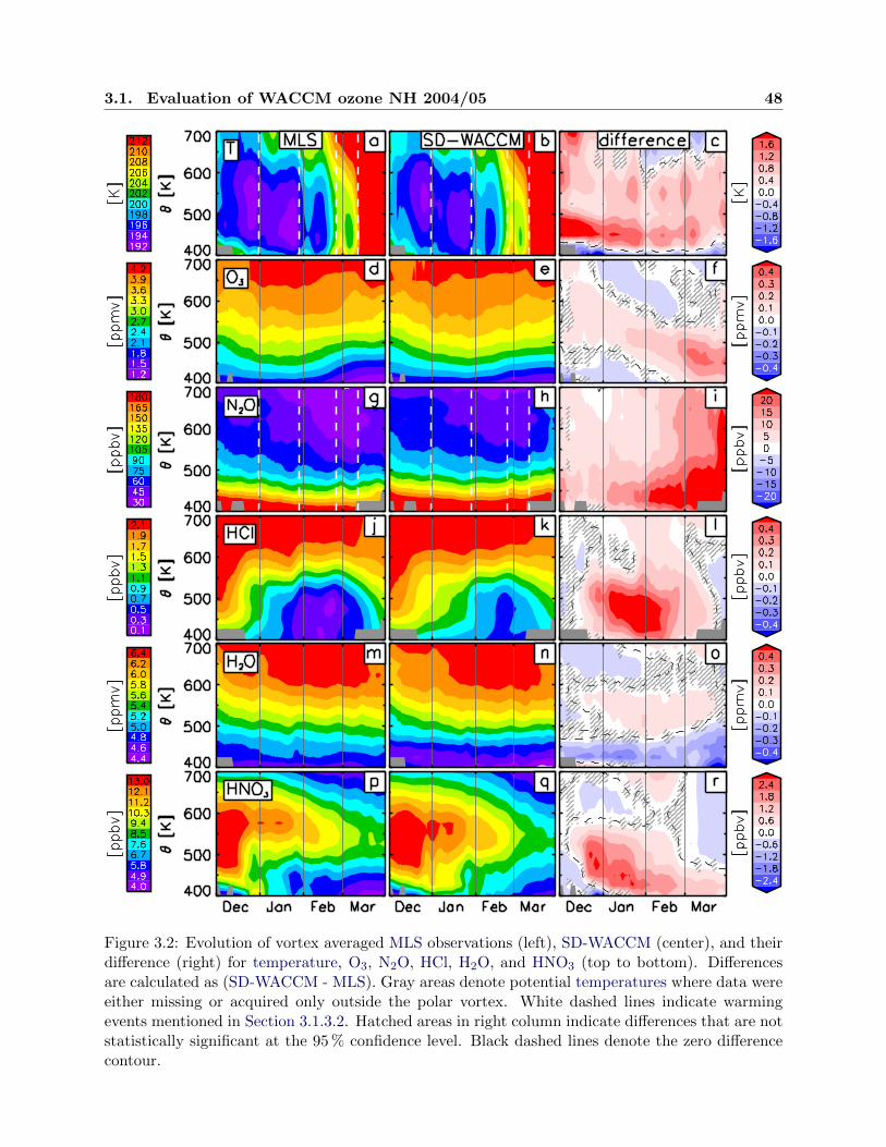
3.1. Evaluation of WACCM ozone NH 2004/05 48
Figure 3.2: Evolution of vortex averaged MLS observations (left), SD-WACCM (center), and theirdifference (right) for temperature, O3, N2O, HCl, H2O, and HNO3 (top to bottom). Differencesare calculated as (SD-WACCM - MLS). Gray areas denote potential temperatures where data wereeither missing or acquired only outside the polar vortex. White dashed lines indicate warmingevents mentioned in Section 3.1.3.2. Hatched areas in right column indicate differences that are notstatistically significant at the 95 % confidence level. Black dashed lines denote the zero differencecontour.
3.1. Evaluation of WACCM ozone NH 2004/05 49
3.1.3.1 Temperature
SD-WACCM is nudged with GEOS5 temperatures, so lower stratospheric SD-WACCM tem-
peratures differ from GEOS5 temperatures only insignificantly (not shown). MLS temperatures are
shown in Figure 3.2a, SD-WACCM (equivalently, GEOS5) temperatures are shown in Figure 3.2b,
and the differences between the two are shown in Figure 3.2c. Morphologically the temperatures
are quite similar, and differences are usually less than ±2 K. At polar latitudes and between 100 hPa
and 17 hPa, the validation of MLS version 3.3 temperature shows differences (GEOS5 minus MLS)
of -0.5±0.3 K to +1.5±0.6 K [Livesey , 2011; Schwartz et al., 2008]. Although small, the impact
of these temperature differences on heterogeneous chemistry is significant; this is discussed in Sec-
tion 3.1.4.2. Here the evolution of simulated and observed temperature is discussed in the context
of dynamics only. PW activity causes deceleration of the zonal wind and thus a warming below
the forcing region [Shepherd , 2000]. Such temperature increases are evident throughout the entire
potential temperature range of 400-700 K in late December through early January, late January, in
the second half of February through early March, and during the final warming around 10 March.
All of these warmings are equally pronounced in the observations and SD-WACCM. The largest
statistically significant temperature differences occur in December and January below the 500 K
isentropic surface, with SD-WACCM overestimating temperatures by up to 3 K relative to MLS. In
general GEOS5 and thus SD-WACCM temperatures are higher than MLS temperatures, a point
that is further discussed in Section 3.1.4.2.
3.1.3.2 Ozone
The evolution of NH polar vortex O3 during the winter of 2004-2005 from MLS and SD-
WACCM is shown in Figure 3.2d and Figure 3.2e. The overall morphology of O3 as simulated by
SD-WACCM is in good agreement with that observed by MLS. Figure 3.2f shows that differences
never exceed 0.35 ppmv; this corresponds to differences that are generally less than 15 %. Small
(mostly statistically insignificant) differences on day 1 of the simulation are caused in part by an
3.1. Evaluation of WACCM ozone NH 2004/05 50
inexact match between the actual MLS data and the gridded product used to initialize SD-WACCM.
The inexact match on day 1 is due to the 7-day running average as well as the spatial smoothing
explained in Section 3.1.2.
Figure 3.3 illustrates the O3 variability within the vortex in more detail for the 475 K po-
tential temperature level. Here the solid red (black) curve represents vortex mean SD-WACCM
(MLS) O3 mixing ratios during the 2004-2005 winter; shaded areas show the vortex mean ±1σ.On
any given day the number of MLS profiles averaged is between ≈ 100 and ≈ 500. The standard
deviation shown in Figure 3 reflects spatial variations inside the polar vortex. The model and
measurements both show increasing O3 mixing ratios until late January, followed by decreases
throughout February and early March. SD-WACCM mixing ratios begin to diverge from MLS
mixing ratios in late January, with differences reaching about 0.35 ppmv (≈ 13 %) by mid March.
Part of this deviation is caused by the small high bias of ≈ 0.1 ppmv seen in Figure 2f above 500 K
in early December, which descends throughout the season. We attribute the December high bias to
a deficiency in the initialization procedure for O3. The remainder of the difference between MLS
and SD-WACCM seen in Figure 2f in March below 500 K is attributed to errors in chemistry as
explained in section 3.4. The model shows considerably less variation inside the vortex than MLS,
as indicated by the narrower shaded area in the model in Figure 3; but the 1s distribution in the
model strongly overlaps the 1s distribution in the observations until early March. Based on the un-
derlying distributions producing the averages, the Wilcoxon signedrank test shows that differences
between vortex-averaged MLS and SD-WACCM O3 mixing ratios are statistically significant after
late January. Thus, Figures 2d-2f and 3 indicate that SD-WACCM in general overestimates O3
during the Arctic 2004-2005 winter in the primary O3 loss region inside the polar vortex below ≈ 525
K. To investigate the reasons behind this overestimate, diagnostics of transport and chemistry are
evaluated in the following sections.
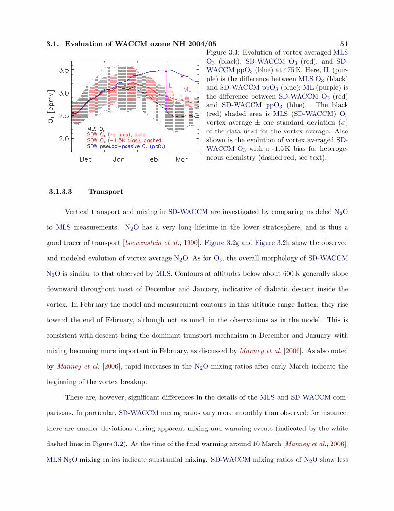
3.1. Evaluation of WACCM ozone NH 2004/05 51Figure 3.3: Evolution of vortex averaged MLSO3 (black), SD-WACCM O3 (red), and SD-WACCM ppO3 (blue) at 475 K. Here, IL (pur-ple) is the difference between MLS O3 (black)and SD-WACCM ppO3 (blue); ML (purple) isthe difference between SD-WACCM O3 (red)and SD-WACCM ppO3 (blue). The black(red) shaded area is MLS (SD-WACCM) O3
vortex average ± one standard deviation (σ)of the data used for the vortex average. Alsoshown is the evolution of vortex averaged SD-WACCM O3 with a -1.5 K bias for heteroge-neous chemistry (dashed red, see text).
3.1.3.3 Transport
Vertical transport and mixing in SD-WACCM are investigated by comparing modeled N2O
to MLS measurements. N2O has a very long lifetime in the lower stratosphere, and is thus a
good tracer of transport [Loewenstein et al., 1990]. Figure 3.2g and Figure 3.2h show the observed
and modeled evolution of vortex average N2O. As for O3, the overall morphology of SD-WACCM
N2O is similar to that observed by MLS. Contours at altitudes below about 600 K generally slope
downward throughout most of December and January, indicative of diabatic descent inside the
vortex. In February the model and measurement contours in this altitude range flatten; they rise
toward the end of February, although not as much in the observations as in the model. This is
consistent with descent being the dominant transport mechanism in December and January, with
mixing becoming more important in February, as discussed by Manney et al. [2006]. As also noted
by Manney et al. [2006], rapid increases in the N2O mixing ratios after early March indicate the
beginning of the vortex breakup.
There are, however, significant differences in the details of the MLS and SD-WACCM com-
parisons. In particular, SD-WACCM mixing ratios vary more smoothly than observed; for instance,
there are smaller deviations during apparent mixing and warming events (indicated by the white
dashed lines in Figure 3.2). At the time of the final warming around 10 March [Manney et al., 2006],
MLS N2O mixing ratios indicate substantial mixing. SD-WACCM mixing ratios of N2O show less

3.1. Evaluation of WACCM ozone NH 2004/05 52
pronounced changes associated with the warming events. Throughout March modeled N2O mixing
ratios increase gradually and relatively smoothly. The final warming is captured appropriately in
the simulation, as expected since the meteorology is nudged to GEOS5 data.
Differences between MLS and SD-WACCM N2O are quantified in Figure 3.2i. On 1 December
differences are below about +10 % (SD-WACCM>MLS). Differences on this date reflect deficiencies
in the initialization. As shown in Table 3.1, SD-WACCM is not initialized with MLS data below
550 K, which explains the overestimate below 500 K. The overestimate at higher altitudes likely
results from discrepancies that arise from the initialization procedure. Because of these initial
disagreements, differences between MLS and SD-WACCM N2O mixing ratios are interpreted here
in a relative sense, focusing on their temporal evolution, not absolute values.
Figure 3.2i shows increasingly positive N2O differences (SD-WACCM>MLS) in late Febru-
ary and early March in particular. Over the course of the season descent is gradually replaced by
isentropic mixing as the dominant transport process [Manney et al., 2006] and thus becomes less
important for controlling constituent distributions. The most likely explanation for these positive
differences, therefore, is errors in the SD-WACCM specification of isentropic mixing. At the alti-
tudes shown here, N2O mixing ratios are lower inside the vortex than outside. Thus an overestimate
of N2O mixing ratios inside the vortex would be consistent with too much SD-WACCM mixing
across the vortex edge.
That SD-WACCM overestimates mixing across the vortex edge is supported by Figure 3.4,
which shows N2O profiles versus equivalent latitude in the descent-dominated early season (5 De-
cember, first column), in the mixingdominated late season (10 March, third column), and in between
(20 January, second column). Equivalent analyses are shown for MLS (top row) and SD-WACCM
(bottom row). Changes in N2O that occurred in the first half of the season are shown by the
differences plotted in Figure 3.4d (Figure 3.4i) for MLS (SD-WACCM). These differences indicate
strong descent, as shown by a decrease in volume mixing ratio inside the polar vortex. The in-
crease outside the polar vortex is caused by extra-vortex advection or mixing (see below). The
N2O plots for MLS and SD-WACCM on 5 December and 20 January are very similar in character,
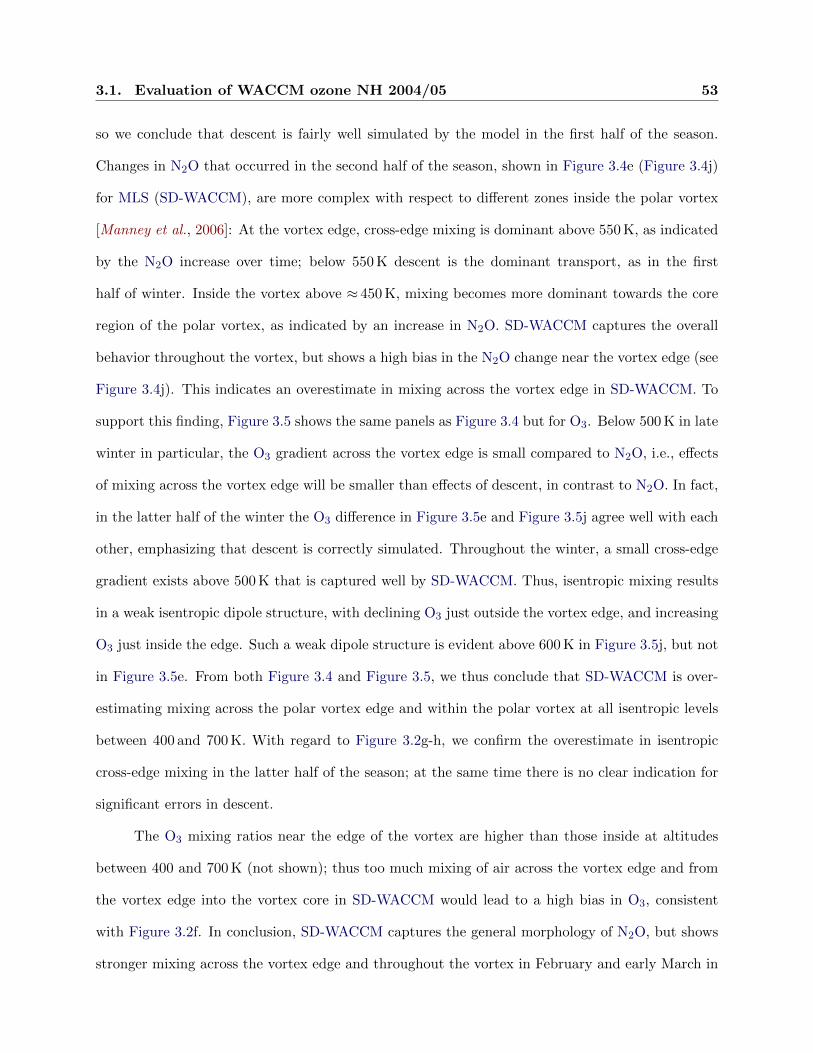
3.1. Evaluation of WACCM ozone NH 2004/05 53
so we conclude that descent is fairly well simulated by the model in the first half of the season.
Changes in N2O that occurred in the second half of the season, shown in Figure 3.4e (Figure 3.4j)
for MLS (SD-WACCM), are more complex with respect to different zones inside the polar vortex
[Manney et al., 2006]: At the vortex edge, cross-edge mixing is dominant above 550 K, as indicated
by the N2O increase over time; below 550 K descent is the dominant transport, as in the first
half of winter. Inside the vortex above ≈ 450 K, mixing becomes more dominant towards the core
region of the polar vortex, as indicated by an increase in N2O. SD-WACCM captures the overall
behavior throughout the vortex, but shows a high bias in the N2O change near the vortex edge (see
Figure 3.4j). This indicates an overestimate in mixing across the vortex edge in SD-WACCM. To
support this finding, Figure 3.5 shows the same panels as Figure 3.4 but for O3. Below 500 K in late
winter in particular, the O3 gradient across the vortex edge is small compared to N2O, i.e., effects
of mixing across the vortex edge will be smaller than effects of descent, in contrast to N2O. In fact,
in the latter half of the winter the O3 difference in Figure 3.5e and Figure 3.5j agree well with each
other, emphasizing that descent is correctly simulated. Throughout the winter, a small cross-edge
gradient exists above 500 K that is captured well by SD-WACCM. Thus, isentropic mixing results
in a weak isentropic dipole structure, with declining O3 just outside the vortex edge, and increasing
O3 just inside the edge. Such a weak dipole structure is evident above 600 K in Figure 3.5j, but not
in Figure 3.5e. From both Figure 3.4 and Figure 3.5, we thus conclude that SD-WACCM is over-
estimating mixing across the polar vortex edge and within the polar vortex at all isentropic levels
between 400 and 700 K. With regard to Figure 3.2g-h, we confirm the overestimate in isentropic
cross-edge mixing in the latter half of the season; at the same time there is no clear indication for
significant errors in descent.
The O3 mixing ratios near the edge of the vortex are higher than those inside at altitudes
between 400 and 700 K (not shown); thus too much mixing of air across the vortex edge and from
the vortex edge into the vortex core in SD-WACCM would lead to a high bias in O3, consistent
with Figure 3.2f. In conclusion, SD-WACCM captures the general morphology of N2O, but shows
stronger mixing across the vortex edge and throughout the vortex in February and early March in
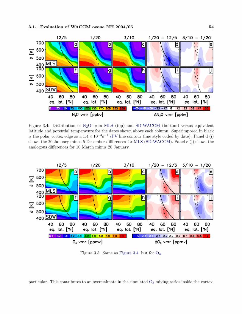
3.1. Evaluation of WACCM ozone NH 2004/05 54
Figure 3.4: Distribution of N2O from MLS (top) and SD-WACCM (bottom) versus equivalentlatitude and potential temperature for the dates shown above each column. Superimposed in blackis the polar vortex edge as a 1.4× 10⁻⁴s−1 sPV line contour (line style coded by date). Panel d (i)shows the 20 January minus 5 December differences for MLS (SD-WACCM). Panel e (j) shows theanalogous differences for 10 March minus 20 January.
Figure 3.5: Same as Figure 3.4, but for O3.
particular. This contributes to an overestimate in the simulated O3 mixing ratios inside the vortex.
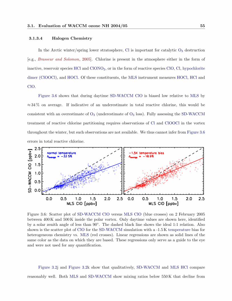
3.1. Evaluation of WACCM ozone NH 2004/05 55
3.1.3.4 Halogen Chemistry
In the Arctic winter/spring lower stratosphere, Cl is important for catalytic O3 destruction
[e.g., Brasseur and Solomon, 2005]. Chlorine is present in the atmosphere either in the form of
inactive, reservoir species HCl and ClONO2, or in the form of reactive species ClO, Cl, hypochlorite
dimer (ClOOCl), and HOCl. Of these constituents, the MLS instrument measures HOCl, HCl and
ClO.
Figure 3.6 shows that during daytime SD-WACCM ClO is biased low relative to MLS by
≈ 34 % on average. If indicative of an underestimate in total reactive chlorine, this would be
consistent with an overestimate of O3 (underestimate of O3 loss). Fully assessing the SD-WACCM
treatment of reactive chlorine partitioning requires observations of Cl and ClOOCl in the vortex
throughout the winter, but such observations are not available. We thus cannot infer from Figure 3.6
errors in total reactive chlorine.
Figure 3.6: Scatter plot of SD-WACCM ClO versus MLS ClO (blue crosses) on 2 February 2005between 400 K and 500 K inside the polar vortex. Only daytime values are shown here, identifiedby a solar zenith angle of less than 90◦. The dashed black line shows the ideal 1:1 relation. Alsoshown is the scatter plot of ClO for the SD-WACCM simulation with a -1.5 K temperature bias forheterogeneous chemistry vs. MLS (red crosses). Linear regressions are shown as solid lines of thesame color as the data on which they are based. These regressions only serve as a guide to the eyeand were not used for any quantification.
Figure 3.2j and Figure 3.2k show that qualitatively, SD-WACCM and MLS HCl compare
reasonably well. Both MLS and SD-WACCM show mixing ratios below 550 K that decline from
3.1. Evaluation of WACCM ozone NH 2004/05 56
December into February, and then increase throughout March. The decline is steeper in MLS
than in SD-WACCM, however, resulting in the high bias in SD-WACCM mixing ratios evident in
Figure 3.2l in December-February below about 550 K. As an example, at 450 K MLS shows a decline
in HCl of ≈ 94 %, whereas SD-WACCM shows a decline of ≈ 69 %. By late February, therefore,
HCl mixing ratios at 450 K in SD-WACCM are higher than those measured by MLS by more than
50 %. We attribute the overestimate below 550 K to errors in chemistry, as described in the next
two paragraphs.
The overall decline that is observed in HCl from January to February is caused primarily
by heterogeneous processing of HCl. Based on observations from both MLS and the Atmospheric
Chemistry Experiment Fourier Transform Spectrometer (ACE-FTS), [Santee et al., 2008] found
that before the onset of Cl activation, HCl at 490 K in the 2004-2005 Arctic winter vortex repre-
sented ≈ 75 % of ClY . Heterogeneous processing led to a decline in HCl so that by late January it
represented only ≈ 10 % of ClY . That HCl in SD-WACCM declines less than in the observations
is thus consistent with too little heterogeneous processing in SD-WACCM, which would lead to an
underestimate of Cl activation. This might explain part of the overestimate in O3 that is evident
in Figure 3.2f, since an underestimate of Cl activation would lead to less chemical loss.
A possible factor contributing to the overestimate of HCl by SD-WACCM is an error in Cl
reservoir partitioning. Studies have shown that the ClONO2 abundance entering winter is rapidly
converted to active chlorine by heterogeneous reactions on STS (and to a lesser extent NAT) by the
reactions of ClONO2 with HCl and H2O [Portmann et al., 1996]. Once the pre-winter ClONO2 is
depleted, additional HCl will not be significantly depleted until later in the winter, when photolytic
processes reform ClONO2. In this work, prewinter ClONO2 is not initialized with observations due
to scarcity of data on 1 December 2004. There is some indication that the model ClONO2 is biased
low (≈ 0.2-0.4 ppbv) in early winter, below 500 K, relative to ACE-FTS observations (not shown).
However, the scarcity of ClONO2 data limits this conclusion. The possible low bias in model
ClONO2 is not yet understood, but is most likely related to the uncertainty in the ClONO2 gas-
phase reaction kinetics, along with possible errors in transport that may lead to an underestimate
3.1. Evaluation of WACCM ozone NH 2004/05 57
of prewinter abundances of inorganic chlorine and inorganic nitrogen. All other things being equal,
such an underestimate will lead to too little chlorine activation, and thus too much O3 (too little
O3 loss), consistent with the results in Figure 3.2.
As mentioned previously, this version of SD-WACCM includes a parameterization of HCl
solubility in STS [Lowe and MacKenzie [2008]; Wegner et al., 2013b]. This parameterization is
highly dependent on the local water vapor abundance and temperature. Wegner et al. [2013b] have
shown that a temperature sensitivity of ±1 K centered at 188 K, with a H2O abundance of 4.5 ppmv,
will change the fraction of HCl in the solution phase to the gas-phase from 25 % (-1 K) to 0 % (+1 K).
In addition, assuming the atmospheric temperature is 188 K, the sensitivity of a ±0.5 ppmv H2O
abundance centered at 4.5 ppmv will change this same fraction from 20 % (+0.5 ppmv) to 0 % (-
0.5 ppmv). Therefore, a high bias in temperature or a low bias in H2O vapor will shift the HCl
equilibrium from the solution to the gas-phase, thus contributing to the overestimate of modeled
HCl. Modeled HCl condensation in this winter does not exceed a polar vortex average of 6 pptv in
late January below 500 K (not shown), which corresponds to a maximum of ≈ 0.5 % of total HCl
in the condensed phase.
3.1.3.5 PSC Formation
The ratio between inactive and reactive Cl is determined in part by the PSC surface area,
since heterogeneous chemistry on the surfaces of primarily STS particles converts inactive Cl to the
photoreactive intermediate Cl2; per convention, we refer to this process as heterogeneous chlorine
activation. Subsequent photolysis of Cl2 then provides Cl for the catalytic O3 destruction cycles
[Solomon, 1999]. PSC particles in general are formed by uptake of H2O and HNO3, which can lead
to permanent dehydration and denitrification if the PSC particles freeze and grow large enough to
sediment. Errors in simulating H2O or HNO3 can thus indicate errors in simulating the PSC SAD,
which would then lead to errors in Cl activation and O3 loss if SAD was the rate limiting property.
Thus, comparisons of MLS and SD-WACCM H2O and HNO3 can be useful for probing errors in
the simulated partitioning between reservoir and active Cl.
3.1. Evaluation of WACCM ozone NH 2004/05 58
Gas-phase H2O from MLS and SD-WACCM, shown in Figure 3.2m-o, compare well; but
there is a small (<7 %) low bias in the model below 475 K and a small (<3 %) high bias above
475 K in December through February. It is possible that the low bias indicates that SD-WACCM
slightly overestimates the uptake of H2O by PSCs. A transient decrease in gas-phase H2O in late
January below 550 K indicates the very brief period with water ice formation described by [Jimenez
et al., 2006], as well as the intrusion of extra-vortex air described by Schoeberl et al. [2006]. The
overall morphology of SD-WACCM gas-phase HNO3 is qualitatively similar to that of MLS, as
shown in Figure 3.2p-r. Quantitatively, however, these comparisons are less favorable than the
H2O comparisons. Below 550 K, SD-WACCM exhibits a high bias in December through February,
with short-term differences up to +30 %. In late January and mid February below ≈ 500 K, both
SD-WACCM and MLS show transient decreases in HNO3 separated by a brief increase, but the
variations are less pronounced in SD-WACCM. The low HNO3 mixing ratios at these times and
altitudes likely represent pulses of increased heterogeneous processing in which gas-phase HNO3 is
taken up by PSCs. These pulses coincide with low temperatures shown in Figure 3.2a-b.
Figure 3.7 shows MLS and SD-WACCM partial columns of gas-phase HNO3 from 400 K
to 700 K. Also shown is the partial column of SD-WACCM condensedphase HNO3 and the MLS
temperature at 550 K. In contrast to Figure 3.2, Figure 3.7 shows column densities, which are
vertically integrated quantities. The lower isentropic levels of Figure 3.2 are weighted more heavily
than higher levels because the atmospheric density decreases with altitude. Therefore some of the
SD-WACCM minus MLS differences that are apparent in Figure 3.2 are not evident in Figure 3.7.
Partial columns of HNO3 are discussed here as opposed to volume mixing ratios in order to show the
total transient exchange between the gas phase and the condensed phase in the lower stratosphere.
This exchange is largely controlled by temperature inside the vortex, but the resulting profiles of
gas- and condensed-phase HNO3 inside the vortex are also determined by the amount of descent.
Therefore, comparisons of mixing ratios and temperatures on individual isentropic levels do not
necessarily provide a self-consistent explanation of physical and chemical processes. For instance,
after PSCs are formed by gas-phase HNO3 uptake, they will descend. This means that atmospheric

3.1. Evaluation of WACCM ozone NH 2004/05 59
temperatures at a lower isentropic level are not necessarily well correlated with condensed-phase
HNO3 that originated at higher altitudes. A similar argument can be made for gas-phase HNO3
because of evaporation of PSCs due to higher temperature at lower levels. Thus, Figure 3.7 adds
to the information that can in part be inferred from Figure 3.2 by showing partial columns rather
than individual isentropic levels. The time series of gas-phase HNO3 partial columns (Figure 3.7)
for SD-WACCM and MLS show very similar relative variations. However, the absolute difference
is consistent with the model’s overestimate of gas-phase HNO3 after mid December that is shown
in Figure 3.2r. The late January and mid February episodic decreases in the partial column of gas-
phase HNO3 are accompanied by increases in condensed phase HNO3 in SD-WACCM and decreases
in temperature, suggesting that those transient declines in gas-phase HNO3 were indeed caused by
PSC uptake. Similarly, the strong anti-correlation from mid December through late February
between SD-WACCM condensed- phase HNO3 and gas-phase HNO3 from both SD-WACCM and
MLS suggests that many of the observed, short-term fluctuations in HNO3 were caused by ongoing
exchanges between the gas and condensed phases.
Figure 3.7: Partial columns (400-700 K) of po-lar vortex averaged gas-phase HNO3 from MLS(black) and SD-WACCM (blue). Also shownis modeled condensed-phase HNO3 (red) andtotal HNO3 (green). Note that the sum ofthe condensed phase HNO3 and the gas phaseHNO3 is exactly the total HNO3. MLS tem-perature at 550 K is superimposed (dashedpurple) following the right ordinate. Alsoshown is SD-WACCM gas-phase HNO3 witha -1.5 K temperature bias for heterogeneouschemistry (gray). A 7-day running average isapplied to all data shown.
Also shown in Figure 3.7 is the total (sum of gas-phase and condensed-phase) HNO3 simulated
by SD-WACCM. The simulated total HNO3 declines gradually by ≈ 40 % throughout January
and February, leveling off in March. This apparent loss of HNO3 is due to diabatic descent and
sedimentation of NAT particles to isentropic levels below 400 K, which is evident from Figure 3.2q
3.1. Evaluation of WACCM ozone NH 2004/05 60
especially in late December through January. Transport from higher altitudes will also decrease
the HNO3 partial column, but not enough to account for the apparent loss shown in Figure 3.7.
Also, isentropic mixing across the vortex edge reduces gas-phase HNO3 inside the vortex because
mixing ratios outside are generally lower between 400 K and 700 K (not shown). There is very
little signature in the total HNO3 of the transient pulse discussed above, while it is noticeable in
the individual condensed-phase and gas-phase time series. This is further confirmation that the
observed, short-term HNO3 variations are simply indicative of an exchange of material between
the gas and condensed phases. By the end of February, SD-WACCM indicates that no more
condensed-phase HNO3 is present; it is likewise reasonable to assume that at this time the MLS
observations of gas-phase HNO3 are about equal to total HNO3 especially since the polar vortex
average temperature is warm enough for most of the condensed-phase HNO3 to evaporate. The
model was initialized with MLS HNO3, yet the total HNO3 is higher in SD-WACCM than in MLS
in March. This reflects a small (<10 %) underestimate by SD-WACCM of HNO3 removal from the
400 K to 700 K vortex region. With the observations shown, however, it is not possible to quantify
errors in the simulated uptake of HNO3 by PSCs, in the estimation of PSC sedimentation, or in
transport/mixing.
3.1.4 Discussion
The differences between SD-WACCM and MLS described in the previous section clearly
have implications for quantifying chemical O3 loss, as mentioned above. This section shows O3
loss calculations based on the pseudo-passive subtraction technique [Singleton et al., 2005]. For
the temperature regime observed in the 2004-2005 Arctic vortex, reaction rates for the reaction of
ClONO2 and HCl on aerosol surfaces are especially sensitive to small temperature variations [e.g.,
Lowe and MacKenzie, 2008]. Hence, this section also discusses the temperature sensitivity of the
O3 loss simulations.
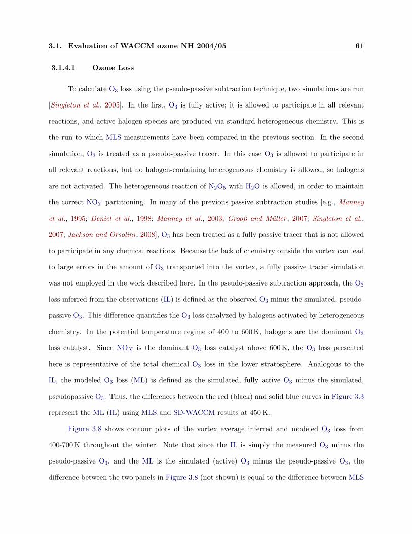
3.1. Evaluation of WACCM ozone NH 2004/05 61
3.1.4.1 Ozone Loss
To calculate O3 loss using the pseudo-passive subtraction technique, two simulations are run
[Singleton et al., 2005]. In the first, O3 is fully active; it is allowed to participate in all relevant
reactions, and active halogen species are produced via standard heterogeneous chemistry. This is
the run to which MLS measurements have been compared in the previous section. In the second
simulation, O3 is treated as a pseudo-passive tracer. In this case O3 is allowed to participate in
all relevant reactions, but no halogen-containing heterogeneous chemistry is allowed, so halogens
are not activated. The heterogeneous reaction of N2O5 with H2O is allowed, in order to maintain
the correct NOY partitioning. In many of the previous passive subtraction studies [e.g., Manney
et al., 1995; Deniel et al., 1998; Manney et al., 2003; Grooß and Muller , 2007; Singleton et al.,
2007; Jackson and Orsolini , 2008], O3 has been treated as a fully passive tracer that is not allowed
to participate in any chemical reactions. Because the lack of chemistry outside the vortex can lead
to large errors in the amount of O3 transported into the vortex, a fully passive tracer simulation
was not employed in the work described here. In the pseudo-passive subtraction approach, the O3
loss inferred from the observations (IL) is defined as the observed O3 minus the simulated, pseudo-
passive O3. This difference quantifies the O3 loss catalyzed by halogens activated by heterogeneous
chemistry. In the potential temperature regime of 400 to 600 K, halogens are the dominant O3
loss catalyst. Since NOX is the dominant O3 loss catalyst above 600 K, the O3 loss presented
here is representative of the total chemical O3 loss in the lower stratosphere. Analogous to the
IL, the modeled O3 loss (ML) is defined as the simulated, fully active O3 minus the simulated,
pseudopassive O3. Thus, the differences between the red (black) and solid blue curves in Figure 3.3
represent the ML (IL) using MLS and SD-WACCM results at 450 K.
Figure 3.8 shows contour plots of the vortex average inferred and modeled O3 loss from
400-700 K throughout the winter. Note that since the IL is simply the measured O3 minus the
pseudo-passive O3, and the ML is the simulated (active) O3 minus the pseudo-passive O3, the
difference between the two panels in Figure 3.8 (not shown) is equal to the difference between MLS
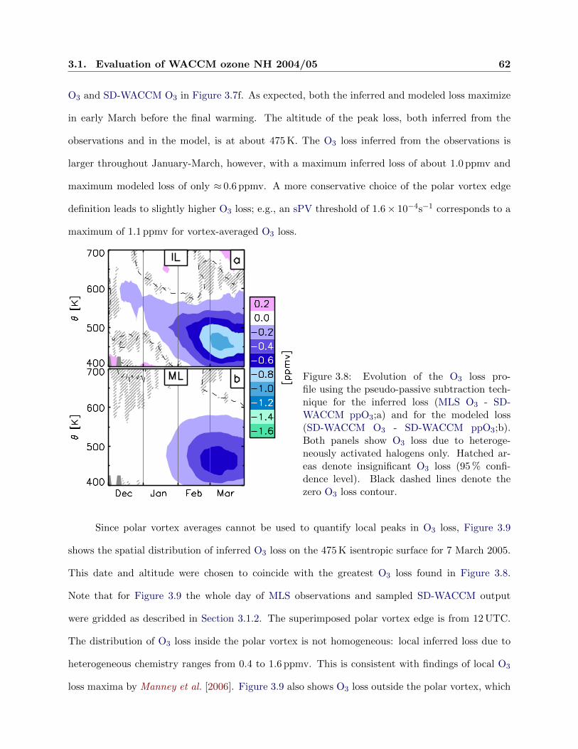
3.1. Evaluation of WACCM ozone NH 2004/05 62
O3 and SD-WACCM O3 in Figure 3.7f. As expected, both the inferred and modeled loss maximize
in early March before the final warming. The altitude of the peak loss, both inferred from the
observations and in the model, is at about 475 K. The O3 loss inferred from the observations is
larger throughout January-March, however, with a maximum inferred loss of about 1.0 ppmv and
maximum modeled loss of only ≈ 0.6 ppmv. A more conservative choice of the polar vortex edge
definition leads to slightly higher O3 loss; e.g., an sPV threshold of 1.6× 10⁻⁴s−1 corresponds to a
maximum of 1.1 ppmv for vortex-averaged O3 loss.
Figure 3.8: Evolution of the O3 loss pro-file using the pseudo-passive subtraction tech-nique for the inferred loss (MLS O3 - SD-WACCM ppO3;a) and for the modeled loss(SD-WACCM O3 - SD-WACCM ppO3;b).Both panels show O3 loss due to heteroge-neously activated halogens only. Hatched ar-eas denote insignificant O3 loss (95 % confi-dence level). Black dashed lines denote thezero O3 loss contour.
Since polar vortex averages cannot be used to quantify local peaks in O3 loss, Figure 3.9
shows the spatial distribution of inferred O3 loss on the 475 K isentropic surface for 7 March 2005.
This date and altitude were chosen to coincide with the greatest O3 loss found in Figure 3.8.
Note that for Figure 3.9 the whole day of MLS observations and sampled SD-WACCM output
were gridded as described in Section 3.1.2. The superimposed polar vortex edge is from 12 UTC.
The distribution of O3 loss inside the polar vortex is not homogeneous: local inferred loss due to
heterogeneous chemistry ranges from 0.4 to 1.6 ppmv. This is consistent with findings of local O3
loss maxima by Manney et al. [2006]. Figure 3.9 also shows O3 loss outside the polar vortex, which
3.1. Evaluation of WACCM ozone NH 2004/05 63
likely arises from mixing across the polar vortex edge: an air parcel can experience O3 loss inside
the polar vortex and then be transported outside the polar vortex. Another possibility, in which
an air parcel containing Cl2 or activated Cl is transported outside the polar vortex, where O3 loss
then occurs, is rather unlikely due to efficient Cl deactivation outside the polar vortex [Douglass
et al., 1991; Lee et al., 2002].
Figure 3.9: Spatial distribution of inferred O3 loss (MLS O3 - SD-WACCM ppO3; left) and modeledO3 loss (SD-WACCM O3 - SD-WACCM ppO3; right) at 475 K on 7 March 2005. The white/blackdashed contour denotes the polar vortex edge as defined by an sPV threshold of 1.4×10⁻⁴s−1. Thered contour line denotes the polar vortex edge using a 1.6× 10⁻⁴s−1 sPV threshold.
As explained above, the most likely factors contributing to the differences between the inferred
and modeled O3 loss are too much mixing across the vortex edge and from the edge into the vortex
core later in the winter, as well as too little halogen activation. In the absence of chemical O3 loss,
lower stratospheric O3 mixing ratios outside the vortex would be lower than inside in late winter
because of more descent inside the vortex. Too much mixing will therefore cause the simulated
pseudo-passive O3 in the lower stratospheric vortex to be underestimated; thus subtracting it from
the observations will result in too little IL. Even though our mixing errors contribute a negative
bias to the simulated O3 in the lower stratosphere late in the winter, the simulated, fully active

3.1. Evaluation of WACCM ozone NH 2004/05 64
O3 mixing ratios are clearly too high (e.g., Figure 3.2f). Thus we conclude that even if mixing
were simulated accurately, the HCl comparisons in late February suggest that SD-WACCM would
underestimate chemical loss because of too little halogen activation. Indeed, the mixing errors are
masking some of the halogen activation error that leads to too little simulated chemical loss.
3.1.4.2 Temperature Sensitivity
Temperatures inside the polar vortex drop sufficiently low for STS and NAT particle for-
mation in the second half of December and January [Lowe and MacKenzie, 2008]. In addition,
localized temperatures are sometimes sufficiently low for small scale water ice particle formation
[Jimenez et al., 2006; Lowe and MacKenzie, 2008]. The temperature differences between MLS
and SD-WACCM that are shown in Figure 3.2c are significant in the context of PSC formation
probabilities and heterogeneous reaction rates. Thus in order to quantify the sensitivity of the O3
loss calculations to temperature variability and possible temperature errors, we repeated the full
chemistry O3 simulation with a temperature bias of -1.5 K for the uptake reaction coefficients for all
STS reactions [Lowe and MacKenzie, 2008; Shi et al., 2001]. Also affected by the temperature bias
is the parameterization of SAD formed by STS and NAT particles, as well as the HCl solubility.
The choice of -1.5 K as a temperature modification for the heterogeneous chemistry in WACCM is
justified by the discrepancies between MLS and SD-WACCM/GEOS5 temperature as discussed in
Section 3.1.3.1 and shown in Figure 3.2c at ≈ 450 K. The temperature modification also falls in the
range of known biases in MLS temperature of -2 to +1 K for isentropic levels between 400 and 700 K
with a precision of ±0.6 to ±0.8 K [Livesey , 2011]. In order to keep modeled dynamics consistent,
the temperature bias is not applied in general but only to reaction coefficients and parameterizations
in the heterogeneous chemistry module, as well as the HCl solubility in SD-WACCM.
Figure 3.10 shows the same comparison as done in Figure 3.2 but applying a -1.5 K tem-
perature bias to heterogeneous processing only. Figure 3.10b-c show this modified temperature.
Observed and modeled O3 agree to within 0.2 ppmv. In addition, the initial high O3 bias that
descends throughout the season, as explained in Section 3.1.3.2, remains at a nearly constant value
3.1. Evaluation of WACCM ozone NH 2004/05 65
of ≈ 0.1 ppmv. Figure 3.4 shows that an overestimate in mixing across the vortex edge does not
significantly increase O3 inside the polar vortex below 500 K, since the cross-edge O3 gradient in
late winter is small. As a tracer N2O is not significantly changed by the temperature bias. In
general, more HCl is heterogeneously processed with the -1.5 K bias, as can be seen from the fact
that the SD-WACCM minus MLS differences are smaller (less positive) with the -1.5 K bias. This
is also supported by an increase in ClO (Figure 3.6, right), improving the averaged underestimate
by SD-WACCM from ≈ 34 % without the temperature bias to ≈ 19 % with the temperature bias.
Modeled HCl condensation with the temperature bias does not exceed a polar vortex average of
32 pptv in late January below 500 K (not shown), which corresponds to a maximum of ≈ 3.5 %
of total HCl in the condensed phase. But the late onset of heterogeneous processing, likely due
to the ClONO2 discrepancy and/or too little condensation of HCl as suggested in Section 3.1.3.4,
is still evident. Note that below 500 K, applying the -1.5 K bias brought the simulated and ob-
served HCl into better agreement. There is a ≤0.35 ppmv low bias in SD-WACCM H2O relative
to MLS (Figure 3.10o) in the region where there is a remaining high bias in HCl (Figure 3.2 and
Figure 3.10), i.e., H2O mixing ratios are independent of the temperature bias. This coupled with
the uncertainty in the laboratory data [Wegner et al., 2013b] used in the parameterization of HCl
condensation could help explain the model high bias in HCl below 500 K. Above 500 K, however,
the simulated HCl is now significantly too low. This makes sense since the temperature bias was
chosen based on the 450 K level as described previously. Figure 3.10 and Figure 3.7 show improve-
ment of modeled gas-phase HNO3, especially from mid January to the end of the season. From the
improvement of the above-described related diagnostics, we conclude that with the temperature
bias the heterogeneous processing is represented more realistically in the model.
Figure 3.3 shows the effect of a 1.5 K temperature decrease on O3 (dashed, red curve). The
1.5 K negative bias improves the agreement with observations from MLS (black curve) in February
and March. When the temperature bias is applied, the maximum of the polar vortex averaged
ML changes from 0.6 ppmv (shown in Figure 3.8b) to 1.0 ppmv (can be inferred from Figure 3.3,
7 March), which matches the IL. We conclude, therefore, that the parameterization of PSC mi-

3.1. Evaluation of WACCM ozone NH 2004/05 66
Figure 3.10: Same as Figure 3.2, but for SD-WACCM simulation using a -1.5 K temperature biasfor heterogeneous chemistry reactions (see text).
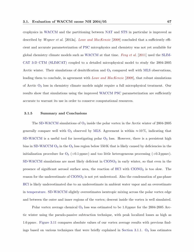
3.1. Evaluation of WACCM ozone NH 2004/05 67
crophysics in WACCM and the partitioning between NAT and STS in particular is improved as
described by Wegner et al. [2013a]. Lowe and MacKenzie [2008] concluded that a sufficiently effi-
cient and accurate parameterization of PSC microphysics and chemistry was not yet available for
global chemistry climate models such as WACCM at that time. Feng et al. [2011] used the SLIM-
CAT 3-D CTM (SLIMCAT) coupled to a detailed microphysical model to study the 2004-2005
Arctic winter. Their simulations of denitrification and O3 compared well with MLS observations,
leading them to conclude, in agreement with Lowe and MacKenzie [2008], that robust simulations
of Arctic O3 loss in chemistry climate models might require a full microphysical treatment. Our
results show that simulations using the improved WACCM PSC parameterization are sufficiently
accurate to warrant its use in order to conserve computational resources.
3.1.5 Summary and Conclusions
The SD-WACCM simulations of O3 inside the polar vortex in the Arctic winter of 2004-2005
generally compare well with O3 observed by MLS. Agreement is within ≈ 10 %, indicating that
SD-WACCM is a useful tool for investigating polar O3 loss. However, there is a persistent high
bias in SD-WACCM O3 in the O3 loss region below 550 K that is likely caused by deficiencies in the
initialization procedure for O3 (+0.1 ppmv) and too little heterogeneous processing (+0.3 ppmv).
SD-WACCM simulations are most likely deficient in ClONO2 in early winter, so that even in the
presence of significant aerosol surface area, the reaction of HCl with ClONO2 is too slow. The
reason for the underestimate of ClONO2 is not yet understood. Also the condensation of gas-phase
HCl is likely underestimated due to an underestimate in ambient water vapor and an overestimate
in temperature. SD-WACCM slightly overestimates isentropic mixing across the polar vortex edge
and between the outer and inner regions of the vortex; descent inside the vortex is well simulated.
Polar vortex average chemical O3 loss was estimated to be 1.0 ppmv for the 2004-2005 Arc-
tic winter using the pseudo-passive subtraction technique, with peak localized losses as high as
1.6 ppmv. Figure 3.11 compares absolute values of our vortex average results with previous find-
ings based on various techniques that were briefly explained in Section 3.1.1. O3 loss estimates
3.1. Evaluation of WACCM ozone NH 2004/05 68
presented here are on the low end of the range of previous results. Vortex edge definitions used in
the studies shown in Figure 3.11, however, were more conservative and thus emphasize O3 loss in
the vortex core more than in this study. A more conservative vortex edge definition is shown in
Figure 3.9 as the red line and corresponding vortex averaged O3 loss results are depicted by the
red profile in Figure 3.11.
Figure 3.11: Comparison of our inferred (modeled) O3 loss results (absolute values) shown assolid (dotted) line, using sPV thresholds of 1.4 × 10⁻⁴s−1 (black) and 1.6 × 10⁻⁴s−1 (red) as thevortex edge definition, with previous research listed in Section 3.1.1: Manney et al. [2006] (M06);Jin et al. [2006a] (J06); Rex et al. [2006] (R06); von Hobe et al. [2006] (H06); Feng et al. [2007a](F07); Grooß and Muller [2007] (G07); Singleton et al. [2007] (S07); Tsvetkova et al. [2007] (T07);El Amraoui et al. [2008] (E08); Jackson and Orsolini [2008] (J08); Rosevall et al. [2008] (R08); andFeng et al. [2011] (F11). Horizontal and vertical lines show the O3 loss range and the altitude rangeover which it was quantified. Blue and green colors as well as linestyles and symbols were chosenfor better legibility and do not have any further meaning. Also shown are standard deviations ofinferred O3 loss results using an sPV threshold of 1.4× 10⁻⁴s−1 (gray).
The temperature sensitivity study in Section 3.1.4.2 shows that the modeled evolution of O3
agrees better with observations when a temperature bias of -1.5 K is imposed on heterogeneous
chemistry reactions and SAD formation. In this case, only the high bias in SD-WACCM O3 of
≈ 0.1 ppmv that is attributed to the initialization procedure remains. Imposing such a temperature
bias, however, does not resolve the late onset of HCl depletion, which is likely due to a ClONO2
deficiency and/or an underestimate of HCl condensation. In order to investigate the ClONO2

3.1. Evaluation of WACCM ozone NH 2004/05 69
deficiency, an in-depth analysis as presented here is planned for several winter seasons in which a
better temporal coverage of ClONO2 observations is available. Such an analysis also evaluates the
interannual variability simulated by WACCM that could not be investigated in this study. Further
work is required to more accurately simulate both isentropic mixing across the vortex edge as well
as heterogeneous chemistry in WACCM.
In conclusion, we have shown through comprehensive model-measurement comparisons that
SD-WACCM reliably simulates most O3 related processes in the Arctic winter of 2004-2005, but
questions remain regarding processes involving chlorine chemistry. Since models differ in, e.g., their
parameterizations of various processes, the results of this study cannot be extrapolated in order
to draw general conclusions about other CCMs and chemical transport models (CTMs). Thus
similar in-depth analyses and model/measurement comparisons or model inter-comparisons, e.g.,
the SPARCs CCMVals Report [SPARC CCMVal , 2010], are necessary to assess other individual
CCMs and CTMs.
Acknowledgments We thank C.S. Singleton for helpful discussions. M.B. and C.E.R.
were funded by JPL/NASA grant 1350080 and NSF award AGS 1135432. The SD-WACCM simu-
lations were carried out at NCAR. NCAR is sponsored by the National Science Foundation. Work
at the Jet Propulsion Laboratory, California Institute of Technology, was done under contract with
the National Aeronautics and Space Administration.

Chapter 4
SD-WACCM simulations of the Antarctic winter 2005
Contents
4.1 Introduction . . . . . . . . . . . . . . . . . . . . . . . . . . . . . . . . . . . . 71
4.2 Method . . . . . . . . . . . . . . . . . . . . . . . . . . . . . . . . . . . . . . . 73
4.3 Evaluation Results . . . . . . . . . . . . . . . . . . . . . . . . . . . . . . . . 75
4.3.1 Temperature . . . . . . . . . . . . . . . . . . . . . . . . . . . . . . . . . . . 76
4.3.2 Ozone . . . . . . . . . . . . . . . . . . . . . . . . . . . . . . . . . . . . . . . 78
4.3.3 Transport . . . . . . . . . . . . . . . . . . . . . . . . . . . . . . . . . . . . 78
4.3.4 Halogen Chemistry . . . . . . . . . . . . . . . . . . . . . . . . . . . . . . . 79
4.3.5 PSC Formation . . . . . . . . . . . . . . . . . . . . . . . . . . . . . . . . . 79
4.3.6 Upper Atmosphere . . . . . . . . . . . . . . . . . . . . . . . . . . . . . . . 82
4.4 Ozone Loss Attribution Results . . . . . . . . . . . . . . . . . . . . . . . . . 83
4.4.1 Dynamical Feedback . . . . . . . . . . . . . . . . . . . . . . . . . . . . . . 84
4.4.2 Ozone Loss Attribution . . . . . . . . . . . . . . . . . . . . . . . . . . . . 85
4.5 Conclusions . . . . . . . . . . . . . . . . . . . . . . . . . . . . . . . . . . . . 88
One of the goals of this study is to attribute separately O3 loss caused by halogens and O3
loss caused by NOX . The main source of stratospheric NOX is oxidation of N2O transported from
the troposphere. But in the middle and upper stratosphere in the polar winter, EPP can also
contribute significantly to NOX [Randall et al., 1998, 2001, 2007]. The largest observed influx of
NOX from EPP to the SH stratosphere occurred in 2000 after the 14 July ”Bastille Day” solar
4.1. Introduction 71
proton event (SPE) [Randall et al., 2001, 2007]. Thus for this investigation we quantify not only
total O3 loss caused by NOX , but also separately quantify O3 loss caused by NOX created by solar
proton (SP) during the SH winter of 2005. Only SPEs that occur during the winter (May-Aug) are
expected to have large effects; since only small or moderate SPEs occurred during these months
in 2005, one would not expect NOX from SPEs to contribute substantially to O3 loss during the
SH 2005 season. It is possible that NOX from precipitating electrons, during the SPEs and/or at
other times during the winter, contributed to the O3 loss observed that winter/spring, but this is
not quantified in this investigation.
A secondary goal of this study is to quantify dynamical feedbacks from O3 experienced by
the experiment simulations: all experiment simulations are done with reduced chemistry, i.e., O3 is
expected to be higher in the experiment simulations compared to the reference simulation resulting
in potential feedback on O3 loss reactions.
4.1 Introduction
Chemical loss of polar stratospheric O3 during the winter seasons is caused by several different
processes. The two most dominant processes are catalytic destruction by halogens and NOX .
Accurately quantifying contributions to O3 loss from these different processes is necessary in order to
understand how stratospheric O3 will evolve under changing atmospheric conditions. For instance,
decreases in stratospheric halogen loading are expected to lead to decreases in halogen-induced
O3 loss [WMO , 2011a]. At the same time, increases in anthropogenic CO2 emissions will cool the
stratosphere [Clough and Iacono, 1995; WMO , 2011a]. This will lead to changes in reaction rates
and circulation that might either increase or decrease O3 loss rates, depending on the particular
process involved.
This chapter describes an investigation of the SH winter of 2005 in which the contributions
to observed changes in stratospheric O3 from individual processes are quantified. The SH 2005
winter is an interesting one in that there were several moderately strong SPEs. Total O3 loss
and halogen-induced O3 loss due to heterogeneous chemistry are quantified, the O3 loss due to all
4.1. Introduction 72
NOX is inferred, and the O3 loss due to NOX created by the SPEs in this winter is quantified.
This study also provides an analysis of dynamical feedback in experiment simulations that have
changed chemistry. The investigation uses CESM/WACCM for a reference simulation matching
observations and two experiment simulations with modified chemistry: the reference simulation
includes full chemistry, in the first experiment simulation heterogeneous chemistry is switched off
as done in Chapter 3 [Brakebusch et al., 2013], and in the second experiment simulation no SPEs
are included. As explained in Section 2.3, O3 loss in the lower stratosphere is dominated by loss
due to halogens, and O3 loss in the upper stratosphere is dominated by catalytic reactions with
NOX . Contributions to the total column O3 loss above the stratosphere are small in an absolute
sense. Hereafter O3 loss quantified as the difference between total O3 loss and halogen-induced O3
loss is thus assumed to be O3 loss due to total NOX . While this is a reasonable assumption, other
O3 loss processes, e.g., HOX -induced O3 loss, are part of what is here called total NOX induced
O3 loss and are not explicitly quantified.
The SH polar vortex generally forms in March and April, and is well established by May. It
often shrinks in September, and is well defined only in the lower half of the stratosphere (i.e., below
≈ 1000 K) in October. In the SH 2005 season, robust conclusions about the upper stratosphere in
October become difficult due to shrinking of the polar vortex and in November robust conclusions
are possible only in the lower stratosphere.
During the SH 2005 winter several SPEs with medium to strong ionization impact occurred
(see Figure 4.1). The strongest SPE occurred in September, and increased NO production all the
way down to the stratopause. However, this NOX was not observed to descend into the middle
stratosphere where it might have contributed significantly to O3 loss [Randall et al., 2007]. EPP
earlier in the winter from other SPEs and other geomagnetic activity produced upper atmospheric
NOX that subsequently descended and reached the stratosphere in June through August. The
total amount of EPP-NOX that descended into the stratosphere in the SH winter of 2005 was
about average for the years 1992-2005 [Randall et al., 2007].
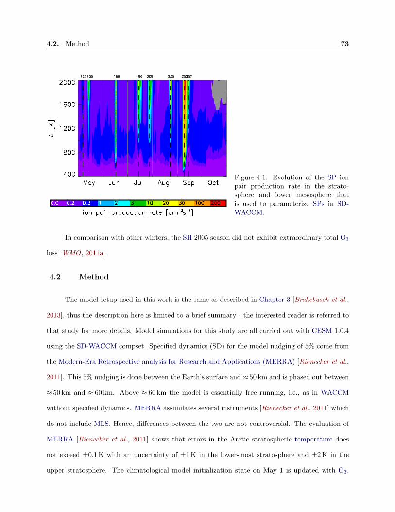
4.2. Method 73
Figure 4.1: Evolution of the SP ionpair production rate in the strato-sphere and lower mesosphere thatis used to parameterize SPs in SD-WACCM.
In comparison with other winters, the SH 2005 season did not exhibit extraordinary total O3
loss [WMO , 2011a].
4.2 Method
The model setup used in this work is the same as described in Chapter 3 [Brakebusch et al.,
2013], thus the description here is limited to a brief summary - the interested reader is referred to
that study for more details. Model simulations for this study are all carried out with CESM 1.0.4
using the SD-WACCM compset. Specified dynamics (SD) for the model nudging of 5% come from
the Modern-Era Retrospective analysis for Research and Applications (MERRA) [Rienecker et al.,
2011]. This 5% nudging is done between the Earth’s surface and ≈ 50 km and is phased out between
≈ 50 km and ≈ 60 km. Above ≈ 60 km the model is essentially free running, i.e., as in WACCM
without specified dynamics. MERRA assimilates several instruments [Rienecker et al., 2011] which
do not include MLS. Hence, differences between the two are not controversial. The evaluation of
MERRA [Rienecker et al., 2011] shows that errors in the Arctic stratospheric temperature does
not exceed ±0.1 K with an uncertainty of ±1 K in the lower-most stratosphere and ±2 K in the
upper stratosphere. The climatological model initialization state on May 1 is updated with O3,
4.2. Method 74
N2O, HCl, H2O, and HNO3 from the EOS MLS (hereafter called MLS) instrument as well as
ClONO2 from the Michelson Interferometer for Passive Atmospheric Sounding (MIPAS) in order
to exactly represent the SH 2005 season. A temperature bias of -1.5 K for heterogeneous chemistry,
SAD calculation, and HCl condensation on STS particles is incorporated in the model to balance
overestimates in MERRA temperature (see Chapter 3 [Brakebusch et al., 2013] and discussion of
Figure 4.2 in Section 4.3 for details). All model output shown in this study is sampled in space
and time to geolocations observed by MLS, unless otherwise noted.
In addition to a reference simulation with full chemistry, two experiment simulations are
carried out. In the first experiment all heterogeneous chemistry is switched off1 . Thus ClOX is
not created and all Cl stays in its reservoir species HCl and ClONO2 (the same is true for Br).
The O3 species in the first experiment simulation is called ppO3. Comparing ppO3 to O3 from the
reference simulation yields a quantification of chemical O3 loss due to halogens that were activated
via heterogeneous chemistry. In the second experiment the ion pair production rate of SPEs is
set to zero. For this simulation low energy (auroral) electrons are not modified; note also that no
medium- or higher energy electrons (i.e., characteristic energy greater than ≈ 30keV) were included
in any of the simulations. The comparison of O3 from this experiment to O3 from the reference
simulation yields a quantification of O3 loss due to additional NOX created by SPs.
In each of the three simulations an ozone tracer (O3TRAC) is included. On the first day (May
1) the O3TRAC is set equal to O3. After May 1 the O3 species and O3TRAC coexist, but O3TRAC
is not involved in any chemistry. It is necessary to have the O3TRAC in addition to the fully active
O3 since the latter provides realistic feedback to the atmosphere (mostly heating by O3 photolysis)
that affects transport of O3TRAC. In order to check whether there is any feedback from the reduced
O3 destruction seen in the pseudo-passive simulation, the O3TRAC species from both the reference
and the experiment are compared. If the differences between O3 tracers are negligible, this indicates
that differences between O3 species from the reference and experimental simulations are truly due to
chemistry only. Using SD-WACCM suppresses unrealistic feedback since temperature changes due
1 Except the reaction N2O5 + H2O −→ 2HNO3 in order to maintain the NOY partitioning

4.3. Evaluation Results 75
to more O3 in the pseudo-passive simulation are compensated by the temperature nudging. Thus
dynamical feedback is reduced in a SD-WACCM experiment simulation. A similar explanation
holds for the second experiment simulation regarding NOX related chemistry.
In this study the subtraction method [Manney et al., 1995] is used to isolate specific aspects
of atmospheric chemistry. The basic concept is to compare a species from a reference model or
observation to an experiment or ”test” simulation in which the parameter of interest is perturbed.
For instance, if chemistry is disabled in the test simulation, the subtraction method allows one to
distinguish between effects of transport (i.e., advection) and chemistry (i.e., chemical creation and
destruction of a species). This technique is then called the passive subtraction method [Manney
et al., 1995]. There are, however, three sources of uncertainties for this method: 1) dynamics in the
model have to be accurate so that differences between the simulated tracer and the reference can be
attributed to chemistry only [e.g., Singleton, 2006]; 2) both the reference species and the modeled
species must start with the same ”atmosphere”; i.e., the model needs to be initialized properly [e.g.,
Singleton et al., 2005]; 3) feedbacks in an experiment simulation influence the species of interest in
an unrealistic way since the experiment involves, e.g., omission of parts of chemistry, and is thus
unrealistic itself; here dynamical as well as chemical feedbacks are possible. All three disadvantages
are addressed in this study: the simulations are nudged with reanalysis data, the model is initialized
with species from the observed atmosphere, and the O3TRAC comparison provides a solution for
dynamical feedbacks. The third concern about passive subtraction methods is not relevant for total
O3 loss since it is calculated as ”O3 minus O3TRAC”, both from the same simulation.
4.3 Evaluation Results
In this Section the evolution of polar vortex averages in the lower stratosphere from MLS
and from the SD-WACCM reference simulation are compared using Figure 4.2.
4.3. Evaluation Results 76
4.3.1 Temperature
From late May through September, the polar vortex average temperature is sufficiently low
(≈ 195K) for PSC type I formation at most altitudes. The polar vortex is coldest in late July with
temperatures below the nominal PSC type II formation threshold of 187 K. Since SD-WACCM
temperature is nudged with MERRA temperature, essentially MERRA temperature is seen in
Figure 4.2b. The nudging covers the entire vertical range shown here. The nudging temperature is
higher than MLS observations.
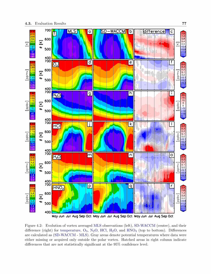
4.3. Evaluation Results 77
Figure 4.2: Evolution of vortex averaged MLS observations (left), SD-WACCM (center), and theirdifference (right) for temperature, O3, N2O, HCl, H2O, and HNO3 (top to bottom). Differencesare calculated as (SD-WACCM - MLS). Gray areas denote potential temperatures where data wereeither missing or acquired only outside the polar vortex. Hatched areas in right column indicatedifferences that are not statistically significant at the 95% confidence level.
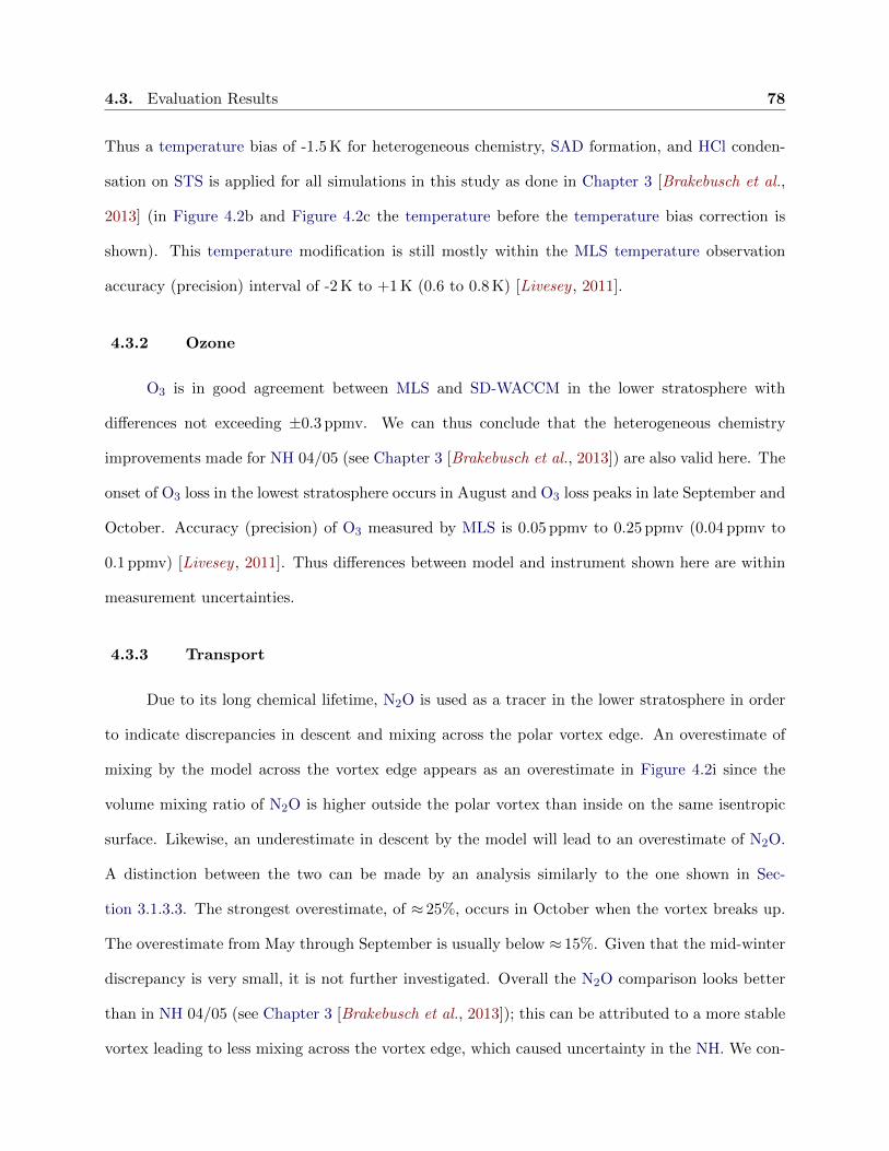
4.3. Evaluation Results 78
Thus a temperature bias of -1.5 K for heterogeneous chemistry, SAD formation, and HCl conden-
sation on STS is applied for all simulations in this study as done in Chapter 3 [Brakebusch et al.,
2013] (in Figure 4.2b and Figure 4.2c the temperature before the temperature bias correction is
shown). This temperature modification is still mostly within the MLS temperature observation
accuracy (precision) interval of -2 K to +1 K (0.6 to 0.8 K) [Livesey , 2011].
4.3.2 Ozone
O3 is in good agreement between MLS and SD-WACCM in the lower stratosphere with
differences not exceeding ±0.3 ppmv. We can thus conclude that the heterogeneous chemistry
improvements made for NH 04/05 (see Chapter 3 [Brakebusch et al., 2013]) are also valid here. The
onset of O3 loss in the lowest stratosphere occurs in August and O3 loss peaks in late September and
October. Accuracy (precision) of O3 measured by MLS is 0.05 ppmv to 0.25 ppmv (0.04 ppmv to
0.1 ppmv) [Livesey , 2011]. Thus differences between model and instrument shown here are within
measurement uncertainties.
4.3.3 Transport
Due to its long chemical lifetime, N2O is used as a tracer in the lower stratosphere in order
to indicate discrepancies in descent and mixing across the polar vortex edge. An overestimate of
mixing by the model across the vortex edge appears as an overestimate in Figure 4.2i since the
volume mixing ratio of N2O is higher outside the polar vortex than inside on the same isentropic
surface. Likewise, an underestimate in descent by the model will lead to an overestimate of N2O.
A distinction between the two can be made by an analysis similarly to the one shown in Sec-
tion 3.1.3.3. The strongest overestimate, of ≈ 25%, occurs in October when the vortex breaks up.
The overestimate from May through September is usually below ≈ 15%. Given that the mid-winter
discrepancy is very small, it is not further investigated. Overall the N2O comparison looks better
than in NH 04/05 (see Chapter 3 [Brakebusch et al., 2013]); this can be attributed to a more stable
vortex leading to less mixing across the vortex edge, which caused uncertainty in the NH. We con-
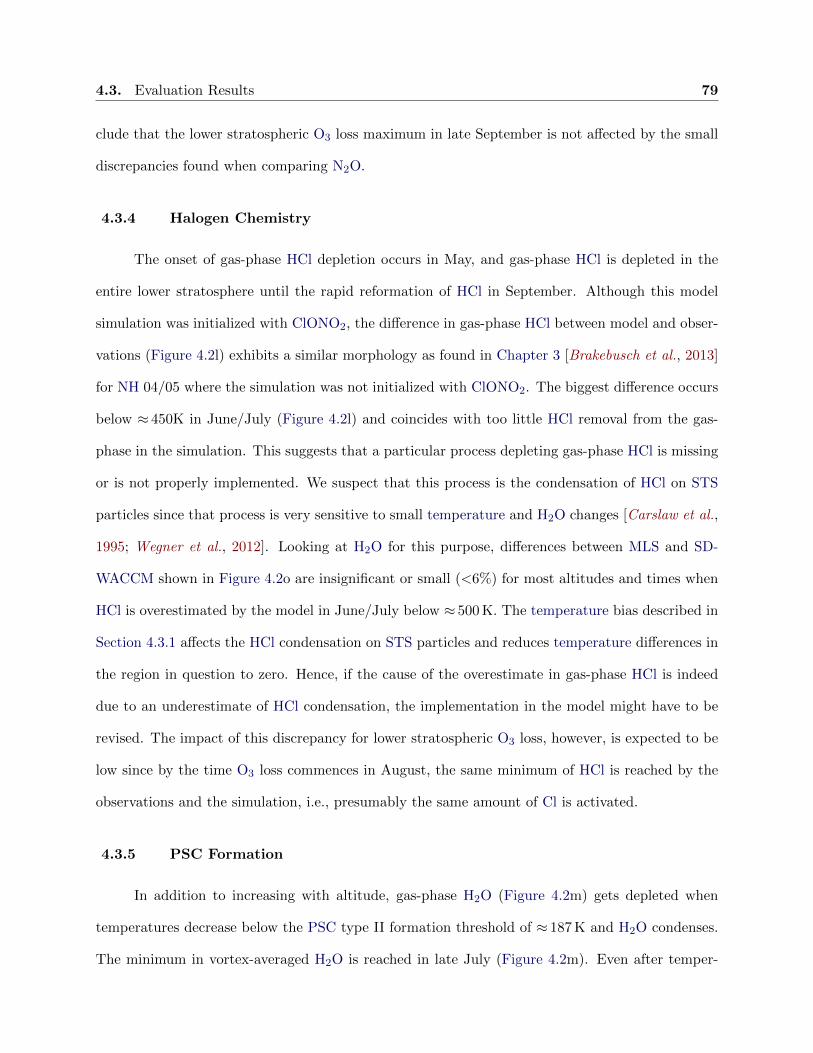
4.3. Evaluation Results 79
clude that the lower stratospheric O3 loss maximum in late September is not affected by the small
discrepancies found when comparing N2O.
4.3.4 Halogen Chemistry
The onset of gas-phase HCl depletion occurs in May, and gas-phase HCl is depleted in the
entire lower stratosphere until the rapid reformation of HCl in September. Although this model
simulation was initialized with ClONO2, the difference in gas-phase HCl between model and obser-
vations (Figure 4.2l) exhibits a similar morphology as found in Chapter 3 [Brakebusch et al., 2013]
for NH 04/05 where the simulation was not initialized with ClONO2. The biggest difference occurs
below ≈ 450K in June/July (Figure 4.2l) and coincides with too little HCl removal from the gas-
phase in the simulation. This suggests that a particular process depleting gas-phase HCl is missing
or is not properly implemented. We suspect that this process is the condensation of HCl on STS
particles since that process is very sensitive to small temperature and H2O changes [Carslaw et al.,
1995; Wegner et al., 2012]. Looking at H2O for this purpose, differences between MLS and SD-
WACCM shown in Figure 4.2o are insignificant or small (<6%) for most altitudes and times when
HCl is overestimated by the model in June/July below ≈ 500 K. The temperature bias described in
Section 4.3.1 affects the HCl condensation on STS particles and reduces temperature differences in
the region in question to zero. Hence, if the cause of the overestimate in gas-phase HCl is indeed
due to an underestimate of HCl condensation, the implementation in the model might have to be
revised. The impact of this discrepancy for lower stratospheric O3 loss, however, is expected to be
low since by the time O3 loss commences in August, the same minimum of HCl is reached by the
observations and the simulation, i.e., presumably the same amount of Cl is activated.
4.3.5 PSC Formation
In addition to increasing with altitude, gas-phase H2O (Figure 4.2m) gets depleted when
temperatures decrease below the PSC type II formation threshold of ≈ 187 K and H2O condenses.
The minimum in vortex-averaged H2O is reached in late July (Figure 4.2m). Even after temper-

4.3. Evaluation Results 80
atures increase to levels high enough for PSC evaporation, H2O remains depleted. SD-WACCM
captures the gas-phase H2O evolution well until September below 500 K (Figure 4.2n); differences
are mostly <10%. After September, H2O below ≈ 500 K is overestimated in the model simulation
by at least 1 ppmv (>25%). This could indicate that too little dehydration via sedimentation of ice
particles occurred during July/August in SD-WACCM, or that there is an error in transport that
masks the sedimentation. The latter is currently investigated at NCAR [personal communication
with Doug Kinnison].
HNO3 is removed from the gas-phase by formation of type I PSCs. When the polar vortex
breaks down, the increasing temperatures evaporate the PSCs if they were not removed from the
stratosphere earlier via sedimentation. The latter is common in the SH due to prolonged cold
temperatures below the type I PSC formation threshold of ≈195 K. The observations (Figure 4.2p)
show a substantial decrease of about 10 ppbv during the season and no immediate recovery of
the gas-phase after the polar vortex gets sufficiently warm for evaporation of PSCs in October
(see Figure 4.2a). We can thus assume substantial denitrification due to sedimentation of PSC
particles. Although the simulation was initialized with HNO3 observations from MLS, significant
model/instrument differences are found in early May. By June, these differences become insignifi-
cant below 550 K and are not exceeding -14% above 550 K. Thus, for the purpose of PSC formation,
these differences are not considered important. Aside from this initial discrepancy, the simulation
(Figure 4.2q) agrees well with the observations throughout the season, but shows a pulse of HNO3
depletion in July and August that is not present in the observations. Since in the simulation HNO3
is restored to the gas-phase in late August below 500 K (Figure 4.2q), even though temperatures
are likely too cold for PSC evaporation, we doubt that the underlying reason for this discrep-
ancy is related to denitrification. The apparent denitrification in July/August is investigated using
Figure 4.3.
Figure 4.3 shows how the spatial distribution across the polar vortex edge evolves over the
course of the season. In the vortex core, i.e., poleward of the −2.0× 10⁻⁴s−1 sPV contour (dashed
line in Figure 4.3), gas-phase HNO3 is completely taken up into PSCs during June. In the outermost

4.3. Evaluation Results 81
Figure 4.3: Evolution of gas-phase HNO3 at 475 K between 40◦ and 90◦ equivalent latitude. Thetop edges of the panels represent the center of the polar vortex. Black lines denote sPV values−2.0 × 10⁻⁴s−1 (dashed) and −1.4 × 10⁻⁴s−1 (solid). The difference contour plot (right) is thedifference between the SD-WACCM (center) and MLS (left) plot.
part of the polar vortex, i.e., between −2.0 × 10⁻⁴s−1 and −1.4 × 10⁻⁴s−1 sPV, gas-phase HNO3
remains as high as before the onset of the denitrification in the polar vortex core as can be seen by
the volume mixing ratio (VMR)s throughout the polar vortex area in May.
Looking back at Figure 4.2p and Figure 4.2q, the vertical structure of gas-phase HNO3 seems
to have descended less in June through August in the model than in the observations as indicated by
the instrument/model difference in the maximum of the HNO3 profile in late July and August. This
is also confirmed by the model slightly overestimating N2O. Given the rather negligible differences
between simulation and observation of gas-phase HNO3 in the polar vortex core (see right panel
of Figure 4.3), we infer that condensed-phase HNO3 is simulated well in the vortex core. We can
thus conclude that condensed-phase HNO3 is not overestimated in the simulation and that the
subsequent denitrification is simulated properly. The latter is confirmed by the small gas-phase
HNO3 differences between model and instrument in September and October (Figure 4.2r). We
thus conclude that despite the low polar vortex average of gas-phase HNO3 the correct amount of
HNO3 is taken up to form PSCs.

4.3. Evaluation Results 82
4.3.6 Upper Atmosphere
In the upper atmosphere, i.e., above ≈ 2500 K (≈55 km), NO2 volume mixing ratios become
very small (not shown). While the morphology of observed NOX is resembled in the simulations,
absolute differences between model and instrument are large above ≈ 4200 K (see difference panel
of Figure 4.4).
Figure 4.4: Evolution of observed (left) and modeled (center) middle and upper atmospheric NOX
in the polar region (latitude < -50◦). The right panel shows the relative difference between observedand simulated NOX . Also shown is the SD-WACCM nudging boundary as a horizontal dashed lineas explained in Section 4.2). The vertical dashed lines indicate the strongest SPEs of this season(see text for details).
Observed NOX increases in June/July and September/October between≈ 2000 K and≈ 4000 K
are of particular importance for O3 related processes since these enhancements of NOX reach the
stratosphere. Without using further diagnostics, it remains unclear whether the underestimate
in June/July is due to insufficient production of NOX or insufficient descent of NOX . As for the
strong SPE in September, the additional NOX in the stratospheric region is overestimated by about
4 ppbv or ≈ 30% (difference panel in Figure 4.4). We can thus expect an overestimate of upper
stratospheric O3 loss in September/October (see O3 loss discussion later) but no effect on chlorine
deactivation, i.e., formation of ClONO2, since the descending air mass with high NOX does not
reach the lower stratosphere.
Since carbon monoxide (CO) is a good tracer for upper atmospheric transport, it is used here
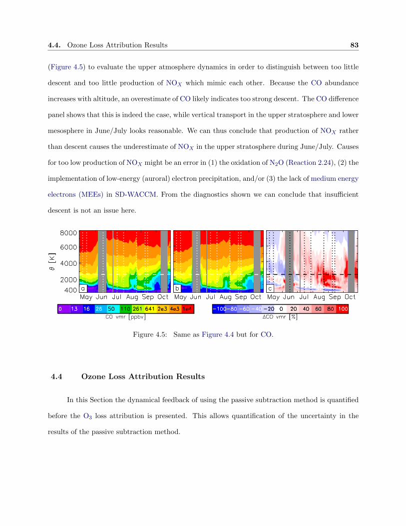
4.4. Ozone Loss Attribution Results 83
(Figure 4.5) to evaluate the upper atmosphere dynamics in order to distinguish between too little
descent and too little production of NOX which mimic each other. Because the CO abundance
increases with altitude, an overestimate of CO likely indicates too strong descent. The CO difference
panel shows that this is indeed the case, while vertical transport in the upper stratosphere and lower
mesosphere in June/July looks reasonable. We can thus conclude that production of NOX rather
than descent causes the underestimate of NOX in the upper stratosphere during June/July. Causes
for too low production of NOX might be an error in (1) the oxidation of N2O (Reaction 2.24), (2) the
implementation of low-energy (auroral) electron precipitation, and/or (3) the lack of medium energy
electrons (MEEs) in SD-WACCM. From the diagnostics shown we can conclude that insufficient
descent is not an issue here.
Figure 4.5: Same as Figure 4.4 but for CO.
4.4 Ozone Loss Attribution Results
In this Section the dynamical feedback of using the passive subtraction method is quantified
before the O3 loss attribution is presented. This allows quantification of the uncertainty in the
results of the passive subtraction method.
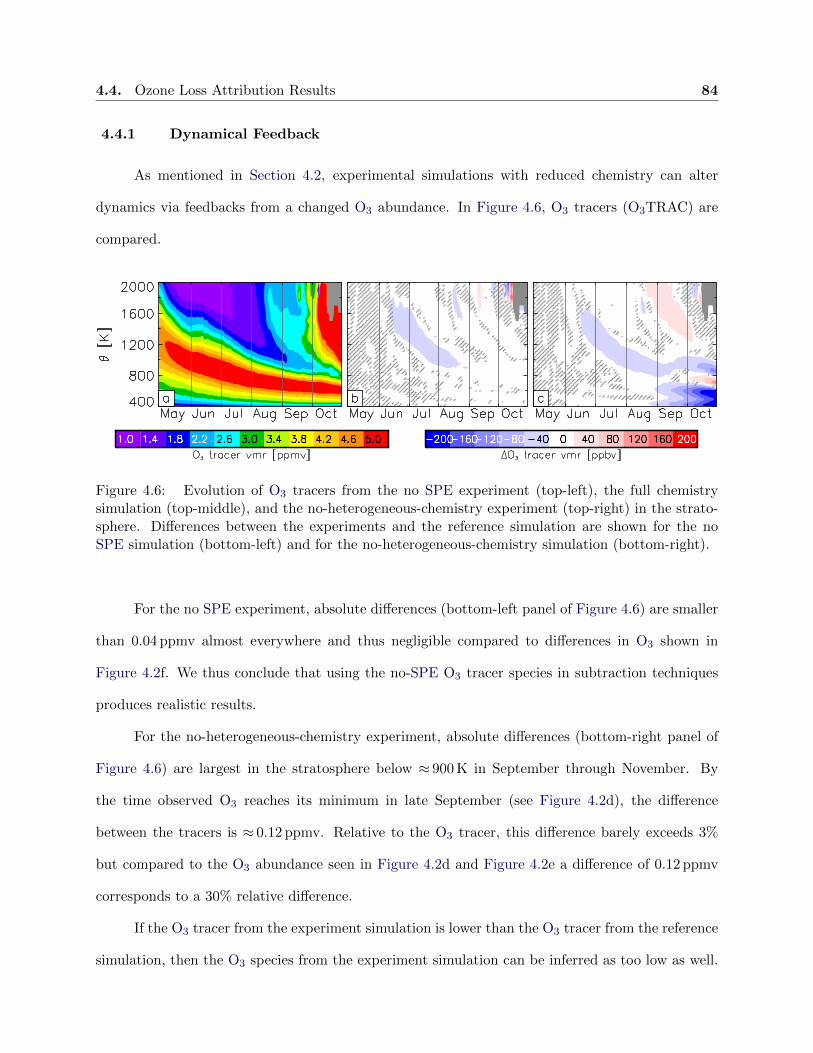
4.4. Ozone Loss Attribution Results 84
4.4.1 Dynamical Feedback
As mentioned in Section 4.2, experimental simulations with reduced chemistry can alter
dynamics via feedbacks from a changed O3 abundance. In Figure 4.6, O3 tracers (O3TRAC) are
compared.
Figure 4.6: Evolution of O3 tracers from the no SPE experiment (top-left), the full chemistrysimulation (top-middle), and the no-heterogeneous-chemistry experiment (top-right) in the strato-sphere. Differences between the experiments and the reference simulation are shown for the noSPE simulation (bottom-left) and for the no-heterogeneous-chemistry simulation (bottom-right).
For the no SPE experiment, absolute differences (bottom-left panel of Figure 4.6) are smaller
than 0.04 ppmv almost everywhere and thus negligible compared to differences in O3 shown in
Figure 4.2f. We thus conclude that using the no-SPE O3 tracer species in subtraction techniques
produces realistic results.
For the no-heterogeneous-chemistry experiment, absolute differences (bottom-right panel of
Figure 4.6) are largest in the stratosphere below ≈ 900 K in September through November. By
the time observed O3 reaches its minimum in late September (see Figure 4.2d), the difference
between the tracers is ≈ 0.12 ppmv. Relative to the O3 tracer, this difference barely exceeds 3%
but compared to the O3 abundance seen in Figure 4.2d and Figure 4.2e a difference of 0.12 ppmv
corresponds to a 30% relative difference.
If the O3 tracer from the experiment simulation is lower than the O3 tracer from the reference
simulation, then the O3 species from the experiment simulation can be inferred as too low as well.
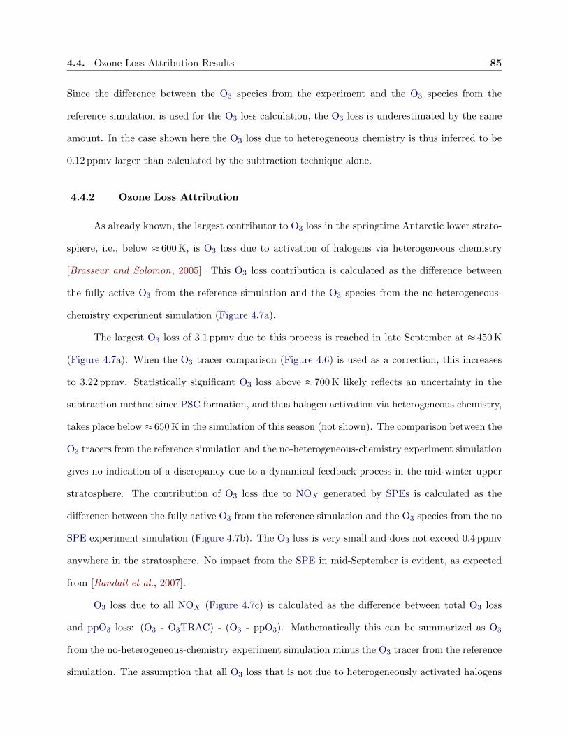
4.4. Ozone Loss Attribution Results 85
Since the difference between the O3 species from the experiment and the O3 species from the
reference simulation is used for the O3 loss calculation, the O3 loss is underestimated by the same
amount. In the case shown here the O3 loss due to heterogeneous chemistry is thus inferred to be
0.12 ppmv larger than calculated by the subtraction technique alone.
4.4.2 Ozone Loss Attribution
As already known, the largest contributor to O3 loss in the springtime Antarctic lower strato-
sphere, i.e., below ≈ 600 K, is O3 loss due to activation of halogens via heterogeneous chemistry
[Brasseur and Solomon, 2005]. This O3 loss contribution is calculated as the difference between
the fully active O3 from the reference simulation and the O3 species from the no-heterogeneous-
chemistry experiment simulation (Figure 4.7a).
The largest O3 loss of 3.1 ppmv due to this process is reached in late September at ≈ 450 K
(Figure 4.7a). When the O3 tracer comparison (Figure 4.6) is used as a correction, this increases
to 3.22 ppmv. Statistically significant O3 loss above ≈ 700 K likely reflects an uncertainty in the
subtraction method since PSC formation, and thus halogen activation via heterogeneous chemistry,
takes place below ≈ 650 K in the simulation of this season (not shown). The comparison between the
O3 tracers from the reference simulation and the no-heterogeneous-chemistry experiment simulation
gives no indication of a discrepancy due to a dynamical feedback process in the mid-winter upper
stratosphere. The contribution of O3 loss due to NOX generated by SPEs is calculated as the
difference between the fully active O3 from the reference simulation and the O3 species from the no
SPE experiment simulation (Figure 4.7b). The O3 loss is very small and does not exceed 0.4 ppmv
anywhere in the stratosphere. No impact from the SPE in mid-September is evident, as expected
from [Randall et al., 2007].
O3 loss due to all NOX (Figure 4.7c) is calculated as the difference between total O3 loss
and ppO3 loss: (O3 - O3TRAC) - (O3 - ppO3). Mathematically this can be summarized as O3
from the no-heterogeneous-chemistry experiment simulation minus the O3 tracer from the reference
simulation. The assumption that all O3 loss that is not due to heterogeneously activated halogens
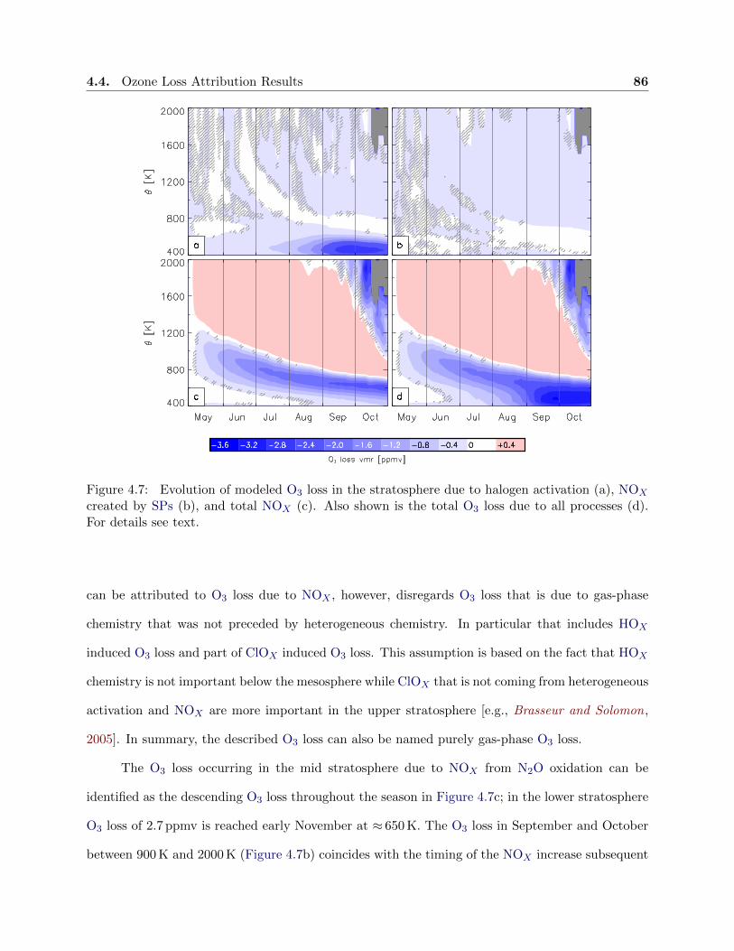
4.4. Ozone Loss Attribution Results 86
Figure 4.7: Evolution of modeled O3 loss in the stratosphere due to halogen activation (a), NOX
created by SPs (b), and total NOX (c). Also shown is the total O3 loss due to all processes (d).For details see text.
can be attributed to O3 loss due to NOX , however, disregards O3 loss that is due to gas-phase
chemistry that was not preceded by heterogeneous chemistry. In particular that includes HOX
induced O3 loss and part of ClOX induced O3 loss. This assumption is based on the fact that HOX
chemistry is not important below the mesosphere while ClOX that is not coming from heterogeneous
activation and NOX are more important in the upper stratosphere [e.g., Brasseur and Solomon,
2005]. In summary, the described O3 loss can also be named purely gas-phase O3 loss.
The O3 loss occurring in the mid stratosphere due to NOX from N2O oxidation can be
identified as the descending O3 loss throughout the season in Figure 4.7c; in the lower stratosphere
O3 loss of 2.7 ppmv is reached early November at ≈ 650 K. The O3 loss in September and October
between 900 K and 2000 K (Figure 4.7b) coincides with the timing of the NOX increase subsequent

4.4. Ozone Loss Attribution Results 87
to the strong SPE event in September (see Figure 4.1 and Figure 4.4), but this O3 loss cannot be
identified in the SPE induced O3 loss (Figure 4.7b). Thus non-SPE NOX is likely the reason for
the increased O3 loss seen here. O3 loss due to NOX from EPPs other than SP is not quantified.
Figure 4.7d combines all O3 loss processes described above and is calculated as the differ-
ence between O3 and O3 tracer, both from the reference simulation. Total O3 loss in the lower
stratosphere reaches 3.6 ppmv in late September at ≈ 480 K. For the UV absorption by O3, the
total number of O3 molecules along the path of the radiation through the atmosphere is important
rather than the volume mixing ratio at any given altitude. Thus the attribution of chemical O3 loss
to individual processes is investigated from a column density point of view in values of DU shown
in Figure 4.8. The inferred total O3 loss (MLS O3 minus reference O3TRAC) in the Antarctic 2005
season reaches a maximum of 158.4 DU in late September.
Figure 4.8: Evolution of inferred (black) andmodeled (green) total chemical O3 column lossbetween 400 K and 3000 K. Also shown are theO3 column losses due to heterogeneous chem-istry (blue), NOX generated by SPEs (red),and total NOX (purple).
Inferred total O3 loss agrees well with modeled total O3 loss of ≈157 DU; the timing of the
simulated O3 loss onset agrees with the observations. In June through August, total O3 loss shown
here is underestimated in the simulations by -5.0 DU± 2.3 DU which corresponds to the small
underestimate of simulated O3 below ≈ 500 K seen in Figure 4.2f. The O3 loss due to halogens
activated by heterogeneous chemistry is as high as 119.5 DU; and the O3 loss due to total NOX
reaches 37.8 DU. As expected from Figure 4.7, O3 loss due to SPE-induced NOX is very low and
only reaches a maximum of 0.47 DU. All maxima occur in late September. After early October
the upper stratospheric vortex breaks up, i.e., the upper part of the column is undefined, which
4.5. Conclusions 88
makes the calculation of the vortex O3 column impossible. In summary, ≈ 76% of the total O3 loss
is due to activated halogens, while the remaining ≈ 24% is caused by NOX from all sources. For
this winter, NOX from SPEs contributed only 0.3% of the total O3 loss (or 1.2% of the total NOX
induced O3 loss).
4.5 Conclusions
Investigating O3 and related species for the SH in this study complements the evaluation of
the NH carried out inChapter 3 [Brakebusch et al., 2013].
Agreement with MLS is in general similar to the results from Chapter 3 [Brakebusch et al.,
2013]: differences in O3 do not exceed ±0.3 ppmv, which is within the uncertainty of MLS obser-
vations; the indicator of descent and mixing, N2O, shows differences smaller than 15%; HCl shows
substantial differences of 0.75 ppbv but reaches the same minimum by the time of the O3 loss onset;
H2O shows agreement within 6% except a late winter model issue; modeled HNO3 underestimates
the observations, but is found to not interfere with the PSC formation; NOX shows too little pro-
duction in the upper atmosphere. We conclude that none of the differences between SD-WACCM
and MLS found in the evaluation have a significant impact for O3 loss investigations. The only
exception is the underestimate of NOX production by EPPs in the upper atmosphere since, via
subsequent descent into the stratosphere, O3 loss by NOX could be increased significantly. We
suggest that the incorporation of MEEs may fix this deficit.
The dynamical feedback from the modified chemistry in the experiment simulations is inves-
tigated: no significant dynamical feedback is found in the no-SPE simulation, but feedback in the
no-heterogeneous-chemistry simulation cannot be neglected. For the latter experiment, a correction
value of 0.12 ppmv is proposed in this winter. The model evaluation shown in Section 4.3 justifies
the O3 loss quantifications since they cannot be evaluated directly. The three O3 loss processes
are quantified: O3 loss due to halogen activation via heterogeneous chemistry is 76%, O3 loss due
to total NOX is 24%, and O3 loss due to NOX created by SPEs during this winter is 0.3%. It
is expected that model improvement, e.g., implementation of MEEs, will increase the total NOX
4.5. Conclusions 89
contribution relative to the halogen contribution. Hence the partitioning given here is valid for
a quiescent winter regarding EPP. Overall we conclude that even if the anthropogenic halogen
loading of the atmosphere reaches zero, at least 24% of the current chemical O3 loss will still occur.
Next to the attribution of glso3 loss processes in the particular SH 2005 winter, this study
contributes the experimental design for attribution studies. In addition an effective way to quantify
errors in dynamical feedback in experiment simulations is developed which addresses the question
raised in Section 2.4 about how to reliably investigate feedback processes.

Chapter 5
SD-WACCM simulations of the Arctic winter 2010/11
Contents
5.1 Introduction . . . . . . . . . . . . . . . . . . . . . . . . . . . . . . . . . . . . 90
5.2 Hypothesis . . . . . . . . . . . . . . . . . . . . . . . . . . . . . . . . . . . . . 91
5.3 Method . . . . . . . . . . . . . . . . . . . . . . . . . . . . . . . . . . . . . . . 93
5.4 Evaluation Results . . . . . . . . . . . . . . . . . . . . . . . . . . . . . . . . 94
5.4.1 Temperature . . . . . . . . . . . . . . . . . . . . . . . . . . . . . . . . . . . 94
5.4.2 Ozone . . . . . . . . . . . . . . . . . . . . . . . . . . . . . . . . . . . . . . . 96
5.4.3 Transport . . . . . . . . . . . . . . . . . . . . . . . . . . . . . . . . . . . . 96
5.4.4 Halogen Chemistry . . . . . . . . . . . . . . . . . . . . . . . . . . . . . . . 97
5.4.5 PSC Formation . . . . . . . . . . . . . . . . . . . . . . . . . . . . . . . . . 98
5.5 Partitioning results . . . . . . . . . . . . . . . . . . . . . . . . . . . . . . . . 98
In this Chapter the unusual Arctic winter of 2010/11 is investigated. Methods for a full study
are described in detail, and preliminary results are shown.
5.1 Introduction
In the Arctic winter season 2010/11 the largest NH O3 loss occurred since the observational
record began [Manney et al., 2011]. In addition to cold temperatures and a prolonged season,
unusual Cl partitioning was observed by, e.g., MLS and MIPAS: while ClONO2 is usually depleted
quickly due to heterogeneous chemistry shortly after the season onset, during the NH 2010/11 season

5.2. Hypothesis 91
ClONO2 was reformed, which commonly occurs only at the end of the season. Since ClONO2 is
usually the rate limiting factor for the reaction with HCl to form Cl2, it determines the amount
of Cl activation. In this winter, however, more than usual Cl activation was observed, possibly
indicating greater availability of ClONO2. The abundance of reactants, however, is not the only
factor influencing Cl activation; in particular temperature and the formation/evaporation of PSCs
play a huge role.
In this study we first evaluate SD-WACCM with MLS and MIPAS for the NH 2010/11 season
using the same approach shown in Chapter 3 [Brakebusch et al., 2013] and Chapter 4. Once the
model/instrument differences are quantified, we investigate the ClY and NOY partitioning using
SD-WACCM. The model complements the observations since the above mentioned instruments can
only provide an incomplete picture regarding species and sampling. This approach is explained in
more detail in Section 2.3. The main question we address in this study is why the observed O3 loss
is high, despite numerous minor warmings that are usually associated with strong isentropic mixing
events across the polar vortex edge, reducing O3 loss. This questions the general assumption that
more stable winter conditions, e.g., as observed in the SH, will lead to more chemical O3 loss.
5.2 Hypothesis
In this study we investigate the chemical interplay during the NH 2010/11 season. We
hypothesize that the large amount of O3 loss was fundamentally caused by transient displacements
of the polar vortex to lower, more sunlit latitudes. Through a complex mechanism, this resulted
in increased Cl activation due to the reformation of ClONO2 (see Section 2.4). The proposed
mechanism is listed below.
(1) The polar vortex is formed by Dec 1, and the temperature inside the polar vortex gets cold
enough to form PSCs in the second half of Dec. This coincides with a decrease in HCl,
indicating formation of Cl2 via Reaction 2.50; a decrease in ClONO2 is expected at the
same time. We can confirm this step by inferring PSC observations by interpreting HNO3
5.2. Hypothesis 92
and H2O observations from MLS, and by investigating the evolution of HCl observations
from MLS as well as ClONO2 observations from MIPAS.
(2) PW activity causes temperature increases in the region of the polar vortex and displaces
the polar vortex (see Section 2.1.2). These displacements to lower latitudes expose the
polar vortex to sunlight several times throughout the season. This step can be confirmed
by investigating the polar vortex temperature and polar vortex position, shape, and size.
All of these can be analyzed using MERRA temperature and derived PV.
(3) The temperature increases described in step 2 cause evaporation of previously formed PSCs;
thus gas-phase HNO3 is increased. Therefore the reaction rate of gas-phase HNO3 pho-
tolysis forming OH and NO2 (λ ≤ 310 nm) is increased when the polar vortex is exposed
to sunlight during a displacement from the pole. Observations of NO2 from MIPAS may
confirm this step; observations of OH from MLS are not available during the time range
investigated here.
(4) NO2 then reacts with previously activated ClO (see Reaction 2.32) and creates ClONO2.
While ClONO2 is reformed, HCl does not increase, which changes the relative partitioning
between the two. This step can be confirmed with ClO observations from MLS and MIPAS,
ClONO2 observations from MIPAS, and HCl observations from MLS.
(5) PSCs reform once the temperature becomes sufficiently low again. Thus gas-phase HNO3
condenses and SAD for heterogeneous chemistry is increased (see Equation 2.57). The
uptake of HNO3 observed by MLS serves as a proxy for PSC formation here.
(6) Subsequently ClONO2 created in step 4 reacts with the remaining HCl on newly formed
PSCs, which increases Cl2 (via Reaction 2.50). The decrease in ClONO2 and HCl can be
confirmed with observations from MIPAS and MLS.
(7) Exposure of the vortex to sunlight photolyzes Cl2 (λ ≤ 350 nm) formed in step 6, and the
O3 loss rate is increased due to Cl-induced catalytic O3 loss. Note that the ”recycled” Cl

5.3. Method 93
atom that was first taken up into ClONO2 (step 4) is reproduced and an additional Cl atom
was released from the HCl reservoir in step 6. Thus, the net result is double the amount
of activated Cl relative to the amount that was removed from the process in step 4. This
step can be confirmed by ClO observations from both MLS and MIPAS.
The net balance of the above described chain is the depletion of twice as many HCl molecules
as ClONO2 molecules. Since there are several minor warmings during this season, this chain of key
processes is expected to repeat several times. In this process the partitioning of ClY shifts from
reservoir Cl towards ClOX , which would not have been possible to the same extent without the
intermediate PSC evaporation/formation and the exposure to sunlight. Thus, if this hypothesis is
confirmed, the increased O3 loss can be partly attributed to the polar vortex variability. The pro-
longed season, however, also contributed to the increased total O3 loss that was observed [Manney
et al., 2011].
Although it is possible to confirm most steps with observations and reanalysis data, a model is
needed to create a representative polar vortex average and to fill in missing species, in particular Cl2.
The work described here uses the WACCM model run in specified dynamics mode (SD-WACCM).
Due to their sun-synchronous, polar orbits, MLS and MIPAS do not sample the polar NH region
at all local times. MLS samples local times from 3 am through 1 pm; MIPAS samples local times
from 10 am through 10 pm. To consistently explain processes in the polar vortex at any given
point in space and time, simultaneous values for all polar vortex constituents are required. This
requirement is fulfilled by using instantaneous or daily averaged output from SD-WACCM. The
simulation used here is first evaluated based on its sampled output (i.e., similar to the evaluation
described in Chapter 3).
5.3 Method
The model is set up in a manner similar to the study in Chapter 3 [Brakebusch et al., 2013].
The simulation is initialized with O3, N2O, H2O, HCl, and HNO3 observations from MLS, nudged
5.4. Evaluation Results 94
with horizontal winds and temperature from MERRA data, and sampled to geolocations from
MLS. Differences are the additional initialization of ClONO2 using MIPAS data (see Chapter 4)
and, in addition to using output sampled to instrument measurement locations, daily averaged
model output are used for the partitioning results.
In the first part, MLS and MIPAS are used to evaluate SD-WACCM with all improvements
made in Chapter 3 [Brakebusch et al., 2013] and Chapter 4. SD-WACCM is compared to MLS
temperature, O3, HCl, and HNO3 as well as to MIPAS ClONO2.
In the second part, the model is used to investigate each step in the hypothesized chain
of processes (see Section 5.2), since the model is independent of instrument sampling and data
availability.
5.4 Evaluation Results
In this Section the evolution of polar vortex averages in the lower stratosphere in MLS
observations is compared to the SD-WACCM reference simulation using Figure 5.1.
5.4.1 Temperature
Observations of polar vortex average temperature (Figure 5.1a) in the NH 2010/11 season
reach minimum values of 192 K. Over the course of the season, however, the low temperature
period is interrupted four times by minor warmings. The onsets (maxima) of the warmings are
early January (Jan 8), end of January (Feb 3), late February (Mar 4), and mid-March (Mar 23).
Figure 5.1b shows SD-WACCM temperature, which is very close to MERRA temperature
due to the nudging (see Chapter 3 [Brakebusch et al., 2013]). However, as described in Chapter 3
[Brakebusch et al., 2013] a temperature bias for heterogeneous chemistry, SAD formation, and HCl
condensation on STS particles is used in this simulation. This modified temperature is shown in
Figure 5.1b. Note that the temperature bias is only applied to part of the chemistry and not to
the entire simulation in order to preserve consistency between nudging temperature and nudging
wind fields.

5.4. Evaluation Results 95
Figure 5.1: Evolution of vortex averaged MLS observations (left), SD-WACCM (center), and theirdifference (right) for temperature, O3, N2O, HCl, H2O, and HNO3 (top to bottom). Differencesare calculated as (SD-WACCM - MLS). Gray areas denote potential temperatures where data wereeither missing or acquired only outside the polar vortex. Hatched areas in right column indicatedifferences that are not statistically significant at the 95% confidence level.
5.4. Evaluation Results 96
Differences between observed and adjusted MERRA temperatures are smallest at the 450 K
level since the temperature bias was chosen so that instrument/model differences at this isentropic
level are zero on seasonal average. The temperature on other isentropic levels is slightly under-
estimated in general due to the temperature bias, but the differences do not exceed -1.2 K where
heterogeneous chemistry is important (425 K - 650 K).
5.4.2 Ozone
The onset of polar vortex average O3 loss takes place in early February; largest O3 loss in the
lower stratosphere is reached by the end of March or early April. The entire period is not covered
by MLS observations due to a temporal data gap between Mar 26 and Apr 19. Assuming that the
largest O3 loss is reached right before the final warming, we can estimate the largest O3 loss to
occur on April 3 (not shown).
The model simulates O3 very well; differences between observations and model are smaller
than ±0.2 ppmv at all isentropic levels in the lower stratosphere until late March. It seems like O3 is
increasingly underestimated between 500 K and 600 K after mid-March, but an exact quantification
is not possible due to the data gap. Extrapolating the morphology of O3 discrepancies for the data
gap in the lowermost stratosphere below 475 K hints at near-zero differences between model and
instrument. Thus we assume that the O3 minimum is correctly simulated.
5.4.3 Transport
In the lower stratosphere, the chemical lifetime of N2O exceeds the timescale of dynamical
processes, so N2O can be used as an indicator of transport [e.g., Brakebusch et al., 2013]. De-
creasing VMRs along all isentropic surfaces until March indicate diabatic descent inside the vortex.
Compared to Figure 3.2 in Chapter 3 and Figure 4.2 in Chapter 4, the diabatic descent in the
NH 2010/11 season appears to be more similar to the SH 2005 season than to the NH 2004/05
season. This confirms the statement by [Manney et al., 2011] that polar dynamics in the NH
2010/11 season are more typical for an SH winter. Increasing VMRs in March and April are an

5.4. Evaluation Results 97
indication of isentropic mixing across the polar vortex edge, since N2O VMRs outside the polar
vortex are higher than inside (not shown). Small changes in the slope of the described contours
coincide with the minor warmings listed in Section 5.4.1. Compared to N2O in the NH 04/05 winter
(see Figure 3.2g-i in Chapter 3), the transient increases in N2O are small, i.e., we can assume that
only minor isentropic mixing with extra-vortex air masses due to the intermediate minor warmings
occurred in the NH 2010/11 season.
The simulation reproduces the morphology of the observations, with differences not exceeding
+16% below 600 K and 33% above 600 K in Dec and Jan. Starting in February, simulated N2O
VMRs gradually increase on isentropic levels below 600 K, overestimating the observations by up
to 40%. A similar behavior was found for the NH 2004/05 season (see Figure 3.2h in Chapter 3)
and the SH 2005 season (see Figure 4.2h in Chapter 4). There, the conclusion was drawn that SD-
WACCM might overestimate isentropic mixing across the polar vortex edge. Since all other species
in Figure 5.1 do not show systematic model/instrument differences beginning in late February
and throughout March, no severe impact on the investigation shown in Section 5.5 is expected.
Chemistry involving the ClY (and NOY ) family converts one family member to another and thus
the total abundance of the family is not changed. Therefore ClY and NOY are susceptible to
changes in dynamics rather than chemistry and can thus be interpreted as tracers. Changes in the
ClY and NOY VMRs in late February and March may thus be interpreted regarding the discrepancy
in mixing diagnosed here.
5.4.4 Halogen Chemistry
Lower stratospheric HCl is rapidly depleted in the second half of December and then reaches
its minimum in late February more gradually. Below 550 K, 92% to 96% of HCl is removed from the
gas-phase and is either activated, transformed into ClONO2, and/or condensed on STS particles.
Again, the highest isentropic level experiencing removal of HCl (≈700 K) is more typical for an
Antarctic season (e.g., Figure 4.2j in Chapter 4) than for an Arctic season (e.g., Figure 3.2j in
Chapter 3) as suggested by Manney et al. [2011]. Around the time of the final warming HCl
5.5. Partitioning results 98
increases and gas-phase VMRs return to pre-winter conditions by mid-April.
The simulation agrees well with the observations, with differences usually not exceeding
±0.2 ppmv. In comparison to the NH 2004/05 study shown in Chapter 3, the model/instrument
discrepancy in the HCl abundance below 500 K in January and February is significantly smaller.
This is attributed to the initialization with ClONO2, which is included for the NH 2010/11 season
but could not be done for the NH 2004/05 season due to availability of observations.
5.4.5 PSC Formation
The comparison of H2O and HNO3 between MLS and SD-WACCM shows differences very
similar to the findings in Chapter 3 [Brakebusch et al., 2013]. Thus the conclusion that SD-WACCM
compares well to MLS is considered to be valid here as well. The model/instrument agreement in
bulk uptake of H2O and HNO3 suggests that a reasonable amount of PSC formation is simulated.
Inferred from transient decreases of gas-phase HNO3, PSCs are assumed to be present in late
December / early January, in the second half of January, and throughout February. The fact that
the gas-phase HNO3 abundance does not return to early winter conditions after the final warming
indicates substantial denitrification. However, Figure 5.1p is inconclusive regarding the timing of
the denitrification that must occur during March until the final warming, i.e., no robust statement
can be made from Figure 5.1p about availability of SAD in March and early April.
5.5 Partitioning results
In this section the evolution of the partitioning of ClY and NOY is investigated in order to
confirm the individual steps of the hypothesis described in Section 5.2. For this purpose Figure 5.2
shows output from the SD-WACCM simulations at 475 K.
According to the simulation of condensed phase HNO3 (light green and cyan lines in middle
panel of Figure 5.2), PSCs are formed in the NH 2010/11 season for the first time in the second
half of December. This coincides with a rapid decrease in HCl and ClONO2 (orange and purple
lines in top panel of Figure 5.2) due to heterogeneous chemistry; only part of this uptake, however,
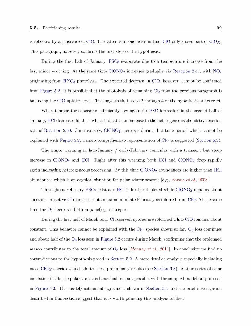
5.5. Partitioning results 99
is reflected by an increase of ClO. The latter is inconclusive in that ClO only shows part of ClOX .
This paragraph, however, confirms the first step of the hypothesis.
During the first half of January, PSCs evaporate due to a temperature increase from the
first minor warming. At the same time ClONO2 increases gradually via Reaction 2.41, with NO2
originating from HNO3 photolysis. The expected decrease in ClO, however, cannot be confirmed
from Figure 5.2. It is possible that the photolysis of remaining Cl2 from the previous paragraph is
balancing the ClO uptake here. This suggests that steps 2 through 4 of the hypothesis are correct.
When temperatures become sufficiently low again for PSC formation in the second half of
January, HCl decreases further, which indicates an increase in the heterogeneous chemistry reaction
rate of Reaction 2.50. Controversely, ClONO2 increases during that time period which cannot be
explained with Figure 5.2; a more comprehensive representation of ClY is suggested (Section 6.3).
The minor warming in late-January / early-February coincides with a transient but steep
increase in ClONO2 and HCl. Right after this warming both HCl and ClONO2 drop rapidly
again indicating heterogeneous processing. By this time ClONO2 abundances are higher than HCl
abundances which is an atypical situation for polar winter seasons [e.g., Santee et al., 2008].
Throughout February PSCs exist and HCl is further depleted while ClONO2 remains about
constant. Reactive Cl increases to its maximum in late February as inferred from ClO. At the same
time the O3 decrease (bottom panel) gets steeper.
During the first half of March both Cl reservoir species are reformed while ClO remains about
constant. This behavior cannot be explained with the ClY species shown so far. O3 loss continues
and about half of the O3 loss seen in Figure 5.2 occurs during March, confirming that the prolonged
season contributes to the total amount of O3 loss [Manney et al., 2011]. In conclusion we find no
contradictions to the hypothesis posed in Section 5.2. A more detailed analysis especially including
more ClOX species would add to these preliminary results (see Section 6.3). A time series of solar
insulation inside the polar vortex is beneficial but not possible with the sampled model output used
in Figure 5.2. The model/instrument agreement shown in Section 5.4 and the brief investigation
described in this section suggest that it is worth pursuing this analysis further.
5.5. Partitioning results 100
Figure 5.2: Evolution of polar vortex averaged ClY partitioning (top), NOY partitioning (middle),and O3, O3TRAC, as well as temperature (bottom) at 475 K. In the middle panel, the sum of allspecies appearing in the legend is approximately the same as NOY before the vortex breaks up. Inthe bottom panel, the difference between O3TRAC (gray) and O3 (black) is the total O3 loss at475 K.

Chapter 6
Conclusions and Outlook
Contents
6.1 Conclusions . . . . . . . . . . . . . . . . . . . . . . . . . . . . . . . . . . . . 101
6.2 Contributions . . . . . . . . . . . . . . . . . . . . . . . . . . . . . . . . . . . 103
6.2.1 Technical contributions . . . . . . . . . . . . . . . . . . . . . . . . . . . . 103
6.2.2 Contributions to science . . . . . . . . . . . . . . . . . . . . . . . . . . . . 104
6.3 Future Plans . . . . . . . . . . . . . . . . . . . . . . . . . . . . . . . . . . . . 108
6.3.1 Additional analysis for the NH 2010/11 study . . . . . . . . . . . . . . 108
6.3.2 Identified but unresolved model deficiencies . . . . . . . . . . . . . . . . 108
6.3.3 Experiment about hypothetical extreme SPEs . . . . . . . . . . . . . . 109
In this chapter the science questions posed in Section 2.4 are answered in the first section;
contributions to the scientific community are listed in the second section. The chapter concludes
with a third section about an outlook on future plans.
6.1 Conclusions
The studies shown in Chapters 3, 4, and 5 answer the science questions posed in Section 2.4.
This section provides these answers as well as embeds them in a greater scientific context.
(1) Is SD-WACCM a tool sophisticated enough for quantitative O3 evolution investigations?
In Chapter 3 [Brakebusch et al., 2013], SD-WACCM is thoroughly evaluated with re-
gard to the evolution of winter polar stratospheric O3. By means of a NH 2004/05 case

6.1. Conclusions 102
study, SD-WACCM is found to be a useful tool to quantify the O3 evolution; remaining
model/instrument discrepancies are identified and explained. The absolute comparison be-
tween observations and SD-WACCM output is mandatory to identify processes that need
improvement in the model. As a further conclusion, accurate temperature is found to be a
key requirement for simulating the effects of heterogeneous chemistry on PSC surfaces. An-
swering the above science question entailed several improvements in SD-WACCM which are
explained in detail in Chapter 3 [Brakebusch et al., 2013] and Section 6.2.2. SD-WACCM is
then used for the SH 2005 season (Chapter 4) and the NH 2010/11 season (Chapter 5) with
results of similar quality. Thus the conclusion that SD-WACCM is a useful tool to quantify
O3 evolution is confirmed. For the scientific community, improving SD-WACCM results
in a well evaluated CCM available for polar stratospheric O3 studies - now SD-WACCM
output of polar stratospheric O3 and related species can be used with confidence.
(2) What are the individual contributions of halogens, NOX from EPP, and NOX from N2O
to O3 loss in the polar vortex?
The SH 2005 season is used in Chapter 4 as a case study because of moderately strong SPE
activity. Separation of the individual processes contributing to O3 loss shows a partitioning
of ≈ 74 % column O3 loss due to halogen chemistry and ≈ 26 % O3 loss due to NOX , of which
< 1 % is due to SPEs. NOX enhancements in the observations that are not simulated are
likely due to the missing MEE implementation in SD-WACCM. For the scientific community
this study enables a quantification of future O3 loss in the mid to late 21st century when
the halogen burden of the stratosphere relaxes back to natural abundances. The method
applied in Chapter 4 can be extended to a quantification of NOX induced O3 loss in
simulations investigating climate change.
(3) Why is the observed O3 loss in the NH 2010/2011 winter so high, despite high dynamical
variability, which is usually associated with less O3 loss?
From the preliminary results shown in Chapter 5 it is inferred that the hypothesized chain
6.2. Contributions 103
of processes (see Section 5.2) is valid: it is suggested that severe O3 loss in the NH 2010/11
can in part be attributed to the atypical intermediate formation of ClONO2 and is not due
to the prolonged season alone. In Section 6.3 improvements to the analysis are described.
6.2 Contributions
Substantial contributions of both a technical and scientific nature are made by the presented
work . This section illustrates these two sets of contributions.
6.2.1 Technical contributions
In order to develop a sophisticated analysis, several technical improvements were necessary
first to streamline the analysis procedure.
As explained in [Brakebusch et al., 2013], a model initialization with data from the instrument
used for the model evaluation is necessary. The technical requirement for this initialization is to
create a gridded data product from the observations to match the model resolution. This procedure
is explained in Appendix A and the implementation is described in [Brakebusch et al., 2013].
In order to evaluate the model with any instrument, the model output must be sampled at
the geolocations, i.e., space and time, observed by the instrument. This is done by means of a
prescribed list of these geolocations, which is called a ”satellite history” file and was developed as
part of this work. This file may contain observed geolocations from several instruments to enable
multiple evaluations. The ”satellite history” file was constantly updated; the current version of the
file, including 37 instruments for the time range of 1970 through present day, contains more than
67 million observations and is also used for the SPARC Earth System Model Validation (ESMVal)
effort. More details about the creation of the satellite history file can be found in Appendix D.
Artificial model tracers were created for NOX , NOY , and O3. Without the latter the attri-
bution of O3 loss (Chapter 4) is not possible. The key characteristic of these tracers is that they
do not replace their chemical equivalent but instead coexist. Thus the simulated atmosphere may
still change the ”active” species and get feedback from the ”active” species; hence the atmosphere
6.2. Contributions 104
remains realistic. This also enables the quantification of feedback errors in experiment simulations
with, e.g., modified chemistry as done in Chapter 4.
Intermediate data products are created during the analysis introduced by [Brakebusch et al.,
2013]. For instance, one of these intermediates contains derived meteorological products, e.g.,
relative vorticity, PV, sPV, equivalent latitude, stream function, and velocity potential. These
quantities are prerequisites for polar vortex definitions and spatial polar coordinates. Use of these
derived meteorological products is not limited to the work shown here, but is applied for other
analyses, e.g., the Concordiasi campaign.
6.2.2 Contributions to science
The scientific interest in polar stratospheric O3 and related processes increased with the dis-
covery of the Antarctic O3 hole. Subsequent WMO reports about O3 depletion summarize advances
in our understanding since 1985. By now most of the processes related to polar stratospheric O3
are understood, thus advances in science became smaller over time. Although atmospheric mod-
els improved greatly over time, the implementation of some processes remains challenging. To
date, state-of-the-art CCMs have not yet achieved the capability to robustly and consistently pre-
dict temperature and O3 loss in the, especially Arctic, polar region for the whole century [e.g.,
Charlton-Perez et al., 2010]. Investigations of diagnostic simulations are thus used to contribute to
the identification, quantification, and improvements of missing details, which lead to the overarching
goal to achieve prediction capability.
This work contributes a sophisticated analysis for CCM simulations of polar stratospheric
O3 and related processes [Brakebusch et al., 2013] to the scientific community. Because of the
interlinked dynamics and chemistry shown in Chapter 2, a comprehensive analysis includes several
key species and in particular discusses temperature accuracy, which was found to be crucial by
[Brakebusch et al., 2013]. This is the first published model/instrument comparison to involve such
a comprehensive evaluation of CCM simulation capabilities of polar stratospheric O3 loss (see
Table 6.1).
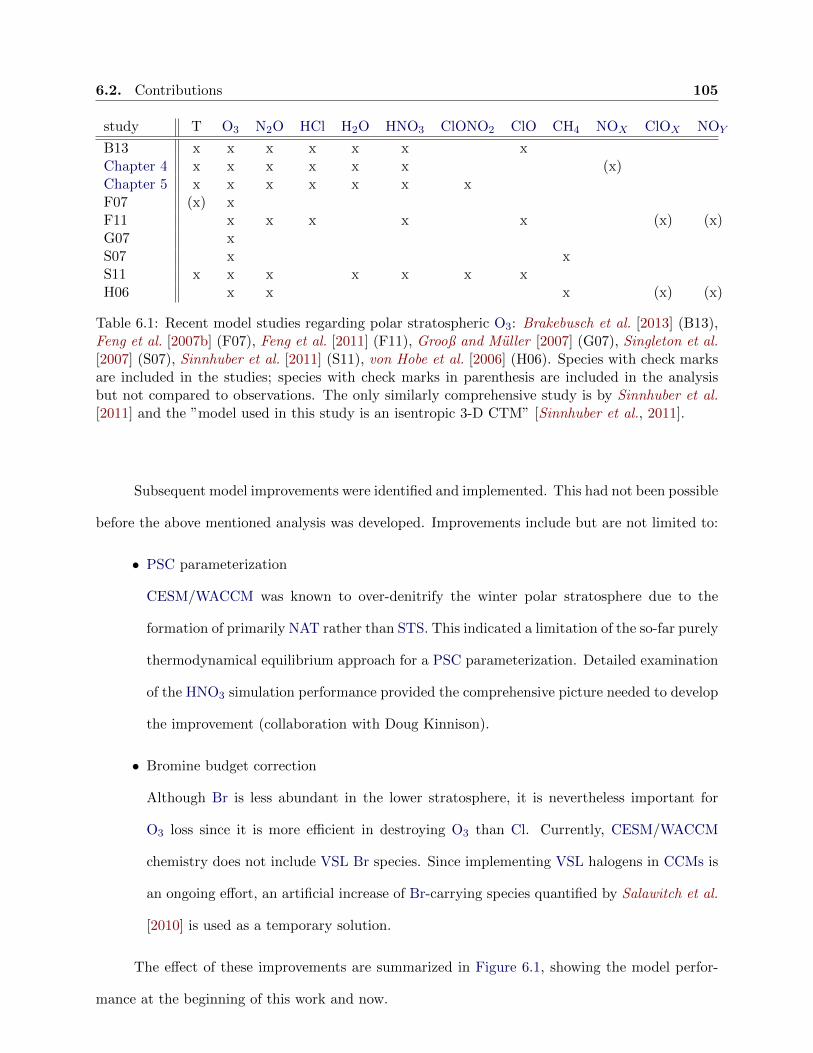
6.2. Contributions 105
study T O3 N2O HCl H2O HNO3 ClONO2 ClO CH4 NOX ClOX NOY
B13 x x x x x x xChapter 4 x x x x x x (x)Chapter 5 x x x x x x xF07 (x) xF11 x x x x x (x) (x)G07 xS07 x xS11 x x x x x x xH06 x x x (x) (x)
Table 6.1: Recent model studies regarding polar stratospheric O3: Brakebusch et al. [2013] (B13),Feng et al. [2007b] (F07), Feng et al. [2011] (F11), Grooß and Muller [2007] (G07), Singleton et al.[2007] (S07), Sinnhuber et al. [2011] (S11), von Hobe et al. [2006] (H06). Species with check marksare included in the studies; species with check marks in parenthesis are included in the analysisbut not compared to observations. The only similarly comprehensive study is by Sinnhuber et al.[2011] and the ”model used in this study is an isentropic 3-D CTM” [Sinnhuber et al., 2011].
Subsequent model improvements were identified and implemented. This had not been possible
before the above mentioned analysis was developed. Improvements include but are not limited to:
• PSC parameterization
CESM/WACCM was known to over-denitrify the winter polar stratosphere due to the
formation of primarily NAT rather than STS. This indicated a limitation of the so-far purely
thermodynamical equilibrium approach for a PSC parameterization. Detailed examination
of the HNO3 simulation performance provided the comprehensive picture needed to develop
the improvement (collaboration with Doug Kinnison).
• Bromine budget correction
Although Br is less abundant in the lower stratosphere, it is nevertheless important for
O3 loss since it is more efficient in destroying O3 than Cl. Currently, CESM/WACCM
chemistry does not include VSL Br species. Since implementing VSL halogens in CCMs is
an ongoing effort, an artificial increase of Br-carrying species quantified by Salawitch et al.
[2010] is used as a temporary solution.
The effect of these improvements are summarized in Figure 6.1, showing the model perfor-
mance at the beginning of this work and now.
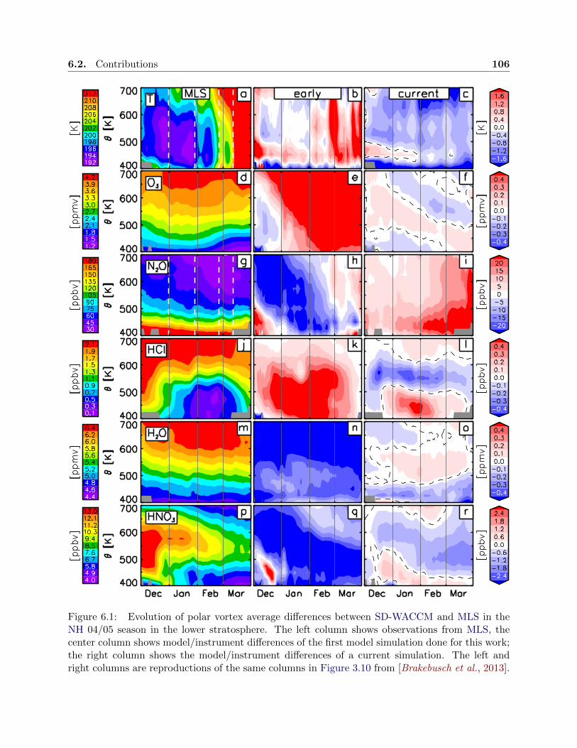
6.2. Contributions 106
Figure 6.1: Evolution of polar vortex average differences between SD-WACCM and MLS in theNH 04/05 season in the lower stratosphere. The left column shows observations from MLS, thecenter column shows model/instrument differences of the first model simulation done for this work;the right column shows the model/instrument differences of a current simulation. The left andright columns are reproductions of the same columns in Figure 3.10 from [Brakebusch et al., 2013].

6.2. Contributions 107
The study presented by [Brakebusch et al., 2013] was necessary to evaluate the previously
described improvements and thus built the foundation for the subsequent studies described in
Chapter 4 and Chapter 5.
The attribution of O3 loss to various processes (Chapter 4) requires simulations with modified
chemistry and the inclusion of O3 tracer species. As examples, simulations without heterogeneous
chemistry and without SPEs were run in order to quantify the individual impact on O3 loss. This
principle is widely used for other chemical questions already. In addition the O3 tracers can be
used to investigate dynamical feedback (Chapter 4) from the chemistry modifications. With the
confidence gained by the first study, both the modified chemistry and the O3 tracer can be trusted.
Thus, the subsequent study (Chapter 4) contributes useful tools needed to investigate attribution
and feedback questions.
As explained by [Brakebusch et al., 2013], the agreement between simulated and observed
gas-phase H2O and HNO3 is a first indication of whether PSC formation is simulated correctly.
The correct amount of uptake (release) from (to) gas-phase bulk material, however, is a necessary
but insufficient requirement for the simulation of PSCs. For instance, particle radii are impor-
tant for denitrification, and particle densities as well as size distribution determine the SAD. In
Chapter 5 the investigation of microphysical parameters used by the parameterization is pursued
via comparison to observations (Cloud-Aerosol Lidar and Infrared Pathfinder Satellite Observation
(CALIPSO)) and explicit microphysics (WACCM/Community Aerosol and Radiation Model for
Atmospheres (CARMA)). The PSC parameterization was evaluated and found to work well re-
garding uptake of H2O and HNO3 [see Brakebusch et al. [2013] and Chapter 4]. The performance
of the PSC parameterization regarding the microphysical parameters listed above is not yet quanti-
fied. Contributing both the evaluation of species uptake and microphysical parameters is expected
to support the development of explicit PSC microphysics.
6.3. Future Plans 108
6.3 Future Plans
In this section some of the still unresolved but necessary model improvements are briefly
described and plans for an experiment showing the theoretically largest possible impact of an
extreme SPE event are outlined.
6.3.1 Additional analysis for the NH 2010/11 study
In Chapter 5 the quality of the PSC parameterization in SD-WACCM is inferred by evaluation
of HNO3 and H2O. But from the quantification of HNO3 and H2O uptake alone the formation of
SAD cannot be calculated. The correct amount of SAD is important because it affects Cl activation
(see Reaction 2.57). In order to simulate SAD in SD-WACCM, a prescribed particle number density
for STS and NAT particles and a constant width of the particle size distribution is used in addition
to the uptake of HNO3 and H2O. The analysis in Chapter 5 will be improved when an evaluation
of the PSC parameterization is included because it supports the discussion of Cl activation.
Considering CALIPSO backscatter observations of PSCs enables an evaluation of the PSC
parameterization used by SD-WACCM. Backscatter from PSC particles can be calculated from the
simulation using the above mentioned parameters. Since the bulk uptake of HNO3 and H2O was
evaluated before (see Section 5.4), differences between simulated and observed backscatter can be
attributed to the calculation of particle size distribution and the number density assumed.
The scientific benefit of this additional analysis is that it provides the basis for further im-
provements of the PSC parameterization while still conserving computational resources compared
to explicit microphysics.
6.3.2 Identified but unresolved model deficiencies
One finding of Chapter 4 is that upper atmospheric NOX is not well simulated in WACCM.
The conclusion in this chapter was insufficient production of NOX by EPP. One reason for this
is that MEE are not represented in SD-WACCM. Another reason is insufficient descent. That is,
6.3. Future Plans 109
NOX created by EPP in the upper atmosphere must descend for stratospheric O3 loss to occur.
This requires a robust simulation of upper atmospheric descent. Smith et al. [2011] concludes that
simulated NOX descent in SD-WACCM might underestimate observations. Some studies suggest
that resolving GWs is a crucial part of improving simulated upper atmospheric circulation and thus
descent, but at the same time resolving this issue is expected to be difficult [e.g., Hamilton et al.,
1999; Shepherd , 2000].
One conclusion of [Brakebusch et al., 2013] was that O3 loss is very sensitive to small tem-
perature changes and that the exact temperature is one of the most crucial requirements for polar
stratospheric O3 simulations of high quality. For the temperature bias on heterogeneous chemistry,
SAD formation, and HCl condensation in CESM/WACCM, a constant value was used in [Brake-
busch et al., 2013], Chapter 4, and Chapter 5. This value represents a polar vortex average fit for
the whole season at one isentropic level only. A change of that bias over the course of the season
or a distinction between vortex core and the outermost vortex area was not made. In order to
reproduce observations better, the temperature bias needs to vary spatially and temporally. This,
however, requires temperature observations with higher accuracy.
6.3.3 Experiment about hypothetical extreme SPEs
In late October 2003, some of the strongest SPE events on record were observed. The ion
pair production rate exceeded the values shown in Chapter 4 by one order of magnitude. Solar
protons penetrated the Earth’s atmosphere down to the stratosphere, and a substantial increase
in NOX and decrease in O3 was observed [Seppala et al., 2004]. This event happened prior to
the onset of the NH polar winter period; increased levels of stratospheric NOX were not observed
anymore by the time the polar vortex formed in December [Funke et al., 2011; Friederich et al.,
2013]. SPEs are unpredictable and sporadic, i.e., this event could have occurred at a later time as
well. Three alternative times of this event are expected to result in completely different impacts
on O3 loss in the stratosphere. First, if the event happened early in the season, e.g., in December,
catalytic O3 loss via the NOX cycle (see Reaction 2.25) is expected in the upper stratosphere
6.3. Future Plans 110
since sunlight is not available for lower stratospheric NOX -induced O3 loss. Also, the formation of
HNO3 via the intermediate N2O5 could increase the HNO3 abundance and thus provide additional
”material” for PSC formation effectively increasing SAD. Secondly, if the event happened during
mid-season when Cl is already activated, the additional NOX may act to deactivate ClOX by the
formation of ClONO2. This then results in an increase of the heterogeneous chemistry reaction rate
of Reaction 2.50 if SAD is still available. Thus a net increase in Cl is expected followed by increased
O3 loss. Thirdly, if the event happened late in the season when SAD is not available anymore, the
formation of ClONO2 would result in the final deactivation of Cl, which greatly reduces O3 loss.
[Brakebusch et al., 2013] and Chapter 5 have shown that CESM/WACCM reproduces the Arctic
atmosphere realistically; and thus it can be expected to simulate the three potential situations
described above with the same quality.

Bibliography
Abarca, J. F., and C. Casiccia (2002), Skin cancer and ultraviolet-B radiation under the Antarcticozone hole: southern Chile, 1987-2000, Photodermatol Photo, 18, 294–302. [cited on page 2.]
Akiyoshi, H., Y. Yamashita, K. Sakamoto, L. B. Zhou, and T. Imamura (2010), Recovery ofstratospheric ozone in calculations by the Center for Climate System Research/National Institutefor Environmental Studies chemistry-climate model under the CCMVal-REF2 scenario and ano-climate-change run, J. Geophys. Res., 115, D19301, doi:10.1029/2009JD012683. [cited onpage 38.]
Andrews, D. G., J. R. Holton, and C. B. Leovy (1987), Middle Atmosphere Dynamics, Interna-tional Geophysics Series, vol. 40, 489 pp., Academic Press, 525 B Street, Suite 1900, San Diego,California 92101-4495. [cited on page 12.]
Bates, D. R., and M. Nicolet (1950), Atmospheric Hydrogen, Publ. Astron. Soc. Pacific, 62, 106.[cited on page 17.]
Bates, T. S., B. K. Lamb, A. Guenther, J. Dignon, and R. E. Stoiber (1992), Sulfur emissions to theatmosphere from natural sources, J. Atmos. Chem., 14 (1-4), 315–337, doi:10.1007/BF00115242.[cited on page 23.]
Blum, U., F. Khosrawi, G. Baumgarten, K. Stebel, R. Muller, and K. H. Fricke (2006), Simultaneouslidar observations of a polar stratospheric cloud on the east and west sides of the Scandinavianmountains and microphysical box model simulations, Ann. Geophys., 24, 3267–3277, doi:10.5194/angeo-24-3267-2006. [cited on page 39.]
Brakebusch, M., C. E. Randall, D. E. Kinnison, S. Tilmes, M. L. Santee, and G. L. Manney (2013),Evaluation of Whole Atmosphere Community Climate Model simulations of ozone during Arcticwinter 2004-2005, J. Geophys. Res.-Atmos., 118 (6), 2673–2688, doi:10.1002/jgrd.50226. [citedon pages 8, 72, 73, 74, 78, 79, 88, 91, 93, 94, 96, 98, 101, 102, 103, 104, 105, 106, 107, 109,110, 125 and 126.]
Brasseur, G., and S. Solomon (2005), Aeronomy of the Middle Atmosphere - Chemistry and Physicsof the Stratosphere and Mesosphere, Atmospheric and Oceanographic Sciences Library, vol. 32,3rd ed., 644 pp., Springer, P.O. Box 17, 3300 AA Dodrecht, The Netherlands, iSBN-10 1-4020-3284-6 (HB) ISBN-13 978-1-4020-3284-4 (HB) ISBN-10 1-4020-3824-0 (e-book) ISBN-13 978-1-4020-3824-1 (e-book). [cited on pages 11, 18, 23, 25, 29, 31, 38, 55, 85 and 86.]
Brasseur, G. P., D. A. Hauglustaine, S. Walters, P. J. Rasch, J. F. Muller, C. Granier, and X. X.Tie (1998), MOZART, a global chemical transport model for ozone and related chemical tracers1. Model description, J. Geophys. Res.-Atmos., 103 (D21), 28,265–28,289. [cited on page 40.]
Brewer, A. W. (1949), Evidence for a world circulation provided by the measurements of heliumand water vapour distribution in the stratosphere, Quart. J. Roy., 75 (326), 351–363, doi:10.1002/qj.49707532603. [cited on page 10.]
Carslaw, K. S., S. L. Clegg, and P. Brimblecombe (1995), A Thermodynamic Model of the SystemHCl-HNO3-H2SO4-H2O, Including Solubilities of HBr, from 200 to 328 K, J. Phys. Chem.,99 (29), 11,557–11,574, doi:10.1021/j100029a039. [cited on pages 24 and 79.]
Carslaw, K. S., T. Peter, and S. L. Clegg (1997), Modeling the composition of liquid stratosphericaerosols, Rev. Geophys., 35 (2), 125–154, doi:10.1029/97RG00078. [cited on page 26.]
Carslaw, K. S., et al. (1998a), Particle microphysics and chemistry in remotely observed moun-tain polar stratospheric clouds, J. Geophys. Res.-Atmos., 103 (D5), 5785–5796, doi:10.1029/97JD03626. [cited on page 25.]
Carslaw, K. S., et al. (1998b), Increased stratospheric ozone depletion due to mountain-inducedatmospheric waves, Nature, 391 (6668), 675–678, doi:10.1038/35589. [cited on page 25.]
Chapman, S. (1930), On ozone and atomic oxygen in the upper atmosphere, Philos. Mag., 10 (64),369–383, doi:10.1080/14786443009461588. [cited on page 15.]
Charlton-Perez, A. J., et al. (2010), The potential to narrow uncertainty in projections ofstratospheric ozone over the 21st century, Atmos. Chem. Phys., 10 (19), 9473–9486, doi:10.5194/acp-10-9473-2010. [cited on pages 1, 5 and 104.]
Charney, J. G., and P. G. Drazin (1961), Propagation of Planetary-Scale Disturbances from Lowerinto Upper Atmosphere, J. Geophys. Res., 66 (1), 83. [cited on page 10.]
Clough, S. A., and M. J. Iacono (1995), Line-By-Line Calculation Of Atmospheric Fluxes AndCooling Rates .2. Application To Carbon-Dioxide, Ozone, Methane, Nitrous-Oxide And TheHalocarbons, J. Geophys. Res.-Atmos., 100 (D8), 16,519–16,535, doi:10.1029/95JD01386. [citedon pages 4 and 71.]
Collins, W. D., et al. (2006), The Formulation and Atmospheric Simulation of the CommunityAtmosphere Model Version 3 (CAM3), J. Climate, 19, 2144–2161, doi:10.1175/JCLI3760.1. [citedon page 40.]
Cox, R. A., W. J. Bloss, R. L. Jones, and D. M. Rowley (1999), OIO and the atmospheric cycle ofiodine, Geophys. Res. Lett., 26 (13), 1857–1860, doi:10.1029/1999GL900439. [cited on page 20.]
Crutzen, P. J. (1970), The influence of nitrogen oxides on the atmospheric ozone content, QuarterlyJournal of the Royal Meteorological Society, 96 (408), 320–325, doi:10.1002/qj.49709640815. [citedon page 19.]
Crutzen, P. J. (1976), Possible Importance of CSO for Sulfate Layer of Stratosphere, Geophys. Res.Lett., 3 (2), 73–76, doi:10.1029/GL003i002p00073. [cited on page 23.]
112
Crutzen, P. J., and F. Arnold (1986), Nitric acid cloud formation in the cold Antarctic stratosphere:a major cause for the springtime ’ozone hole’, Nature, 324 (6098), 651–655. [cited on page 22.]
Crutzen, P. J., I. S. A. Isaksen, and G. C. Reid (1975), Solar Proton Events - StratosphericSources of Nitric-Oxide, Science, 189 (4201), 457–459, doi:10.1126/science.189.4201.457. [citedon page 27.]
Deniel, C., R. M. Bevilacqua, J. P. Pommereau, and F. Lefevre (1998), Arctic chemical ozonedepletion during the 1994-1995 winter deduced from POAMII satellite observations and theREPROBUS three-dimensional model, J. Geophys. Res., 103 (D15), 19,231–19,244, doi:10.1029/98JD01446. [cited on page 61.]
Dessler, A. E., M. D. Burrage, J. U. Grooss, J. R. Holton, J. L. Lean, S. T. Massie, M. R. Schoeberl,A. R. Douglass, and C. H. Jackman (1998), Selected science highlights from the first 5 years ofthe Upper Atmosphere Research Satellite (UARS) Program, Rev. Geophys., 36 (2), 183–210,doi:10.1029/97RG03549. [cited on page 31.]
Dibb, J. E., E. Scheuer, M. Avery, J. Plant, and G. Sachse (2006), In situ evidence for renitrificationin the Arctic lower stratosphere during the polar aura validation experiment (PAVE), Geophys.Res. Lett., 33, L12815, doi:10.1029/2006GL026243. [cited on page 39.]
Dobson, G. M. B. (1956), Origin and Distribution of the Polyatomic Molecules in the Atmosphere,Proc. Roy. Soc. London, 236 (1205), 187–193. [cited on page 10.]
Douglass, A. R., R. B. Rood, J. A. Kaye, R. S. Stolarski, D. J. Allen, and E. M. Larson (1991), Theinflulence of polar heterogeneous processes on reactive chlorine at middle latitudes: Three di-mensional model implications, Geophys. Res. Lett., 18(1), 25–28, doi:10.1029/90GL02601. [citedon page 63.]
Dowdy, S., S. Wearden, and D. Chilko (2004), Statistics for Research, 3 ed., Wiley, Hoboken, NewJersey, USA, iSBN: 978-0-471-26735-5. [cited on page 47.]
Drdla, K., and R. Muller (2012), Temperature thresholds for chlorine activation and ozone lossin the polar stratosphere, Ann. Geophys., 30 (7), 1055–1073, doi:10.5194/angeo-30-1055-2012.[cited on page 45.]
Dunkerton, T. J., and D. P. Delisi (1986), Evolution of Potential Vorticity in the Winter Strato-sphere of January-February 1979, J. Geophys. Res.-Atmos., 91 (D1), 1199–1208. [cited onpage 46.]
Dye, J. E., B. W. Gandrud, D. Baumgardner, K. R. Chan, G. V. Ferry, M. Loewenstein, K. K.Kelly, and J. C. Wilson (1990), Observed particle evolution in the polar stratospheric cloud ofJanuary 24, 1989, Geophys. Res. Lett., 17 (4), 413–416, doi:10.1029/GL017i004p00413. [cited onpage 25.]
Dye, J. E., D. Baumgardner, B. W. Gandrud, S. R. Kawa, K. K. Kelly, M. Loewenstein, G. V. Ferry,K. R. Chan, and B. L. Gary (1992), Particle size distributions in Arctic polar stratospheric clouds,growth and freezing of sulfuric acid droplets, and implications for cloud formation, J. Geophys.Res.-Atmos., 97 (D8), 8015–8034, doi:10.1029/91JD02740. [cited on page 25.]
113

El Amraoui, L., N. Semane, V.-H. Peuch, and M. L. Santee (2008), Investigation of dynamicalprocesses in the polar stratospheric vortex during the unusually cold winter 2004/2005, Geophys.Res. Lett., 35 (3), L03803, doi:10.1029/2007GL031251. [cited on pages 38, 39 and 68.]
Emmons, L. K., et al. (2010), Description and evaluation of the Model for Ozone and Relatedchemical Tracers, version 4 (MOZART-4), Geosci. Model Dev., 3 (1), 43–67. [cited on page 40.]
Esler, J. G., and D. W. Waugh (2002), A method for estimating the extent of denitrification ofArctic polar vortex air from tracer-tracer scatter plots, J. Geophys. Res.-Atmos., 107 (D13),doi:10.1029/2001JD001071. [cited on page 40.]
Fahey, D. W., K. K. Kelly, G. V. Ferry, L. R. Poole, J. C. Wilson, D. M. Murphy, M. Loewenstein,and K. R. Chan (1989), In situ measurements of total reactive nitrogen, total water, and aerosolin a polar stratospheric cloud in the Antarctic, J. Geophys. Res.-Atmos., 94 (D9), 11,299–11,315,doi:10.1029/JD094iD09p11299. [cited on pages 23 and 25.]
Fahey, D. W., K. K. Kelly, S. R. Kawa, A. F. Tuck, M. Loewenstein, K. R. Chan, and L. E. Heidt(1990), Observations of denitrification and dehydration in the winter polar stratospheres, Nature,344 (6264), 321–324, doi:10.1038/344321a0. [cited on page 25.]
Fahey, D. W., et al. (2001), The Detection of Large HNO3-Containing Particles in the Winter ArcticStratosphere, Science, 291 (5506), 1026–1031, doi:10.1126/science.1057265. [cited on page 25.]
Farman, J. C., B. G. Gardiner, and J. D. Shanklin (1985), Large Losses of Total Ozone in AntarcticaReveal Seasonal ClOx/NOx Interaction, Nature, 315 (6016), 207–210. [cited on page 21.]
Feng, W., M. P. Chipperfield, M. Dorf, K. Pfeilsticker, and P. Ricaud (2007a), Mid-latitude ozonechanges: studies with a 3-D CTM forced by ERA-40 analyses, Atmos. Chem. Phys., 7 (9), 2357–2369, doi:10.5194/acp-7-2357-2007. [cited on pages 38 and 68.]
Feng, W., M. P. Chipperfield, S. Davies, P. von der Gathen, E. Kyroe, C. M. Volk, A. Ulanovsky,and G. Belyaev (2007b), Large chemical ozone loss in 2004/2005 Arctic winter/spring, Geophys.Res. Lett., 34 (9), L09803, doi:10.1029/2006GL029098. [cited on page 105.]
Feng, W., M. P. Chipperfield, S. Davies, G. W. Mann, K. S. Carslaw, S. Dhomse, V. L. Harvey,C. E. Randall, and M. L. Santee (2011), Modelling the effect of denitrification on polar ozonedepletion for the Arctic winter 2004/2005, Atmos. Chem. Phys., 11, 6559–6573, doi:10.5194/acp-11-6559-2011. [cited on pages 38, 67, 68 and 105.]
Friederich, F., T. von Clarmann, B. Funke, H. Nieder, J. Orphal, M. Sinnhuber, G. P. Stiller, andJ. M. Wissing (2013), Lifetime and production rate of NOx in the upper stratosphere and lowermesosphere in the polar spring/summer after the solar proton event in October-November 2003,Atmos. Chem. Phys., 13 (5), 2531–2539, doi:10.5194/acp-13-2531-2013. [cited on page 109.]
Fritts, D. C., and M. J. Alexander (2003), Gravity wave dynamics and effects in the middle atmo-sphere, Rev. Geophys., 41 (1), doi:10.1029/2001RG000106. [cited on pages 12 and 13.]
Funke, B., et al. (2011), Composition changes after the ”Halloween” solar proton event: the HighEnergy Particle Precipitation in the Atmosphere (HEPPA) model versus MIPAS data intercom-parison study, Atmos. Chem. Phys., 11 (17), 9089–9139, doi:10.5194/acp-11-9089-2011. [cited onpage 109.]
114

Grooß, J.-U., and R. Muller (2007), Simulation of ozone loss in Arctic winter 2004/2005, Geophys.Res. Lett., 34 (5), L05804, doi:10.1029/2006GL028901. [cited on pages 38, 40, 61, 68 and 105.]
Hamilton, K., R. J. Wilson, and R. S. Hemler (1999), Middle atmosphere simulated with highvertical and horizontal resolution versions of a GCM: Improvements in the cold pole bias andgeneration of a QBO-like oscillation in the tropics, J. Atmos. Sci., 56 (22), 3829–3846. [cited onpage 109.]
Hanson, D., and K. Mauersberger (1988), Laboratory Studies of the Nitric-Acid Trihydrate - Impli-cations for the South Polar Stratosphere, Geophys. Res. Lett., 15 (8), 855–858. [cited on page 25.]
Hauglustaine, D. A., G. P. Brasseur, S. Walters, P. J. Rasch, J.-F. Muller, L. K. Emmons, andC. A. Carroll (1998), MOZART, a global chemical transport model for ozone and related chemicaltracers 2. Model results and evaluation, J. Geophys. Res.-Atmos., 103 (D21), 28,291–28,335, doi:10.1029/98JD02398. [cited on page 40.]
Holton, J. R. (2004), An Introduction to Dynamic Meteorology, vol. 88, 4th ed., 535 pp., AcademicPress, San Diego. [cited on pages 10 and 11.]
Hoppel, K., et al. (2002), POAM III observations of arctic ozone loss for the 1999/2000 winter, J.Geophys. Res.-Atmos., 107 (D20), doi:10.1029/2001JD000476. [cited on page 39.]
Horowitz, L. W., et al. (2003), A global simulation of tropospheric ozone and related tracers:Description and evaluation of MOZART, version 2, J. Geophys. Res.-Oc. Atm., 108 (D24), doi:10.1029/2002JD002853. [cited on page 40.]
IPCC (2007), Climate Change 2007: The Physical Science Basis, Working Group I Report, Cam-bridge University Press. [cited on page 23.]
Jackman, C. H. (1991), Effects of Energetic Particles on Minor Constituents of the Middle Atmo-sphere, J. Geomagn. Geoelectr., 43 (Suppl.)(2, S), 637–646, 7th Quadrennial Solar TerrestrialSymp / 27th Cospar Meeting, The Hague, Netherlands, Jul 25-30, 1990. [cited on page 28.]
Jackson, D. R., and Y. J. Orsolini (2008), Estimation of Arctic ozone loss in winter 2004/05 basedon assimilation of EOS MLS and SBUV/2 observations, Quart. J. Roy., 134 (636, Part A), 1833–1841, doi:10.1002/qj.316. [cited on pages 38, 40, 61 and 68.]
Jackson, D. R., S. J. Driscoll, E. J. Highwood, J. E. Harries, and J. M. Russell (1998), Troposphereto stratosphere transport at low latitudes as studies using HALOE observations of water vapour1992-1997, Quart. J. Roy., 124 (545), 169–192, doi:10.1002/qj.49712454508. [cited on page 18.]
Jimenez, C., H. C. Pumphrey, I. A. MacKenzie, G. L. Manney, M. L. Santee, M. J. Schwartz, R. S.Harwood, and J. W. Waters (2006), EOS MLS observations of dehydration in the 2004-2005 polarwinters, Geophys. Res. Lett., 33 (16), L16806, doi:10.1029/2006GL025926. [cited on pages 39, 58and 64.]
Jin, J. J., et al. (2006a), Severe Arctic ozone loss in the winter 2004/2005: observations from ACE-FTS, Geophys. Res. Lett., 33 (15), L15801, doi:10.1029/2006GL026752. [cited on pages 38, 40and 68.]
Jin, J. J., et al. (2006b), Denitrification in the Arctic winter 2004/2005: Observations from ACE-FTS, Geophys. Res. Lett., 33 (19), doi:10.1029/2006GL027687. [cited on page 39.]
115

Junge, C. E., and J. E. Manson (1961), Stratospheric aerosol studies, J. Geophys. Res., 66 (7),2163–2182, doi:10.1029/JZ066i007p02163. [cited on page 24.]
Junge, C. E., C. W. Chagnon, and J. E. Manson (1961), Stratospheric Aerosols, J. Meteorol., 18,81–108. [cited on page 24.]
Kelly, K. K., et al. (1989), Dehydration in the lower Antarctic stratosphere during late win-ter and early spring, 1987, J. Geophys. Res.-Atmos., 94 (D9), 11,317–11,357, doi:10.1029/JD094iD09p11317. [cited on page 25.]
Kinnison, D. E., et al. (2007), Sensitivity of chemical tracers to meteorological parameters inthe MOZART-3 chemical transport model, J. Geophys. Res.-Atmos., 112 (D20), doi:10.1029/2006JD007879. [cited on pages 40, 45 and 46.]
Kinnison, D. E., et al. (2013), Description and Evaluation of the Specified Dynamics version of theWhole Atmosphere Community Climate Model (SD-WACCM), Geosci. Model Dev., in prepara-tion. [cited on page 34.]
Kleinbohl, A., H. Bremer, H. Kullmann, J. Kuttippurath, E. V. Browell, T. Canty, R. J. Salaw-itch, G. C. Toon, and J. Notholt (2005), Denitrification in the Arctic mid-winter 2004/2005observed by airborne submillimeter radiometry, Geophys. Res. Lett., 32 (19), L19811, doi:10.1029/2005GL023408. [cited on page 39.]
Kley, D., A. L. Schmeltekopf, K. Kelly, R. H. Winkler, T. L. Thompson, and M. McFarland (1982),Transport of water through the tropical tropopause, Geophys. Res. Lett., 9 (6), 617–620, doi:10.1029/GL009i006p00617. [cited on page 17.]
Knuth, D. E. (1992), Axioms and Hulls, Springer-Verlag, Berlin/Heidelberg, Germany. [cited onpages 43 and 123.]
Kunz, A., L. L. Pan, P. Konopka, D. E. Kinnison, and S. Tilmes (2011), Chemical and dynamicaldiscontinuity at the extratropical tropopause based on START08 and WACCM analyses, J.Geophys. Res.-Atmos., 116, D24302, doi:10.1029/2011JD016686. [cited on page 41.]
Lamarque, J.-F., et al. (2012), CAM-chem: description and evaluation of interactive atmosphericchemistry in the Community Earth System Model, Geosci. Model Dev., 5 (2), 369–411, doi:10.5194/gmd-5-369-2012. [cited on pages 40 and 41.]
Leaf, A. (1993), Loss of Stratospheric Ozone and Health Effects of Increased Ultraviolet Radiation,Cambridge, MA: The MIT Press. [cited on page 2.]
Lee, A. M., R. L. Jones, I. Kilbane-Dawe, and J. A. Pyle (2002), Diagnosing ozone loss in the ex-tratropical lower stratosphere, J. Geophys. Res.-Atmos., 107 (D11), doi:10.1029/2001JD000538.[cited on page 63.]
Lin, S. J. (2004), A ”vertically Lagrangian” finite-volume dynamical core for global models, Mon.Weather Rev., 132 (10), 2293–2307, doi:10.1175/1520-0493(2004)132〈2293:AVLFDC〉2.0.CO;2.[cited on page 41.]
Lin, S. J., and R. B. Rood (1996), Multidimensional flux-form semi-Lagrangian transport schemes,Mon. Weather Rev., 124 (9), 2046–2070, doi:10.1175/1520-0493(1996)124〈2046:MFFSLT〉2.0.CO;2. [cited on page 41.]
116
Livesey, e. a., N. J. (2011), Earth Observing System (EOS) Aura Microwave Limb Sounder (MLS)Version 3.3 Level 2 data quality and description document, Tech. rep., Jet Propulsion Laboratory,California Institute of Technology, Pasadena, California. [cited on pages 42, 43, 46, 49, 64, 78and 123.]
Loewenstein, M., J. R. Podolske, K. R. Chan, and S. E. Strahan (1990), N2O as a dynamical tracerin the Arctic vortex, Geophys. Res. Lett., 17 (4), 477–480, doi:10.1029/GL017i004p00477. [citedon pages 30 and 51.]
Lovelock, J. E. (1971), Atmospheric Fluorine Compounds as Indicators of Air Movements, Nature,230 (5293), 379–379, doi:10.1038/230379a0. [cited on page 21.]
Lowe, D., and A. R. MacKenzie (2008), Polar stratospheric cloud microphysics and chemistry, J.Atmos. Terr. Phy., 70 (1), 13–40, doi:10.1016/j.jastp.2007.09.011. [cited on pages 24, 26, 45, 57,60, 64 and 67.]
Manney, G. L., L. Froidevaux, J. W. Waters, and R. W. Zurek (1995), Evolution Of MicrowaveLimb Sounder Ozone And The Polar Vortex During Winter, J. Geophys. Res.-Atmos., 100 (D2),2953–2972. [cited on pages 40, 61 and 75.]
Manney, G. L., J. L. Sabutis, S. Pawson, M. L. Santee, B. Naujokat, R. Swinbank, M. E. Gelman,and W. Ebisuzaki (2003), Lower stratospheric temperature differences between meteorologicalanalyses in two cold Arctic winters and their impact on polar processing studies, J. Geophys.Res.-Atmos., 108 (D5), doi:10.1029/2001JD001149. [cited on page 61.]
Manney, G. L., M. L. Santee, L. Froidevaux, K. Hoppel, N. J. Livesey, and J. W. Waters (2006),EOS MLS observations of ozone loss in the 2004-2005 Arctic winter, Geophys. Res. Lett., 33 (4),L04802, doi:10.1029/2005GL024494. [cited on pages 38, 39, 40, 51, 52, 53, 62 and 68.]
Manney, G. L., et al. (2011), Unprecedented Arctic ozone loss in 2011, Nature, 478 (7370), 469–475,doi:10.1038/nature10556. [cited on pages 34, 36, 90, 93, 96, 97 and 99.]
Matsuno, T. (1971), A Dynamical Model of the Stratospheric Sudden Warming, J. Atmos. Sci.,28 (8), 1479–1494, doi:10.1175/1520-0469(1971)028〈1479:ADMOTS〉2.0.CO;2. [cited on page 11.]
McElroy, M. B., R. J. Salawitch, S. C. Wofsy, and J. A. Logan (1986), Reductions of AntarcticOzone due to Synergistic Interactions of Chlorine and Bromine, Nature, 321 (6072), 759–762.[cited on page 22.]
McInturff, R. (1978), Stratospheric warmings: Synoptic, dynamic and general-circulation aspects,25 tech. rep. nasa-rp-1017, NASA Reference Publ., Washington, DC. [cited on page 12.]
Michelsen, H. A., G. L. Manney, M. R. Gunson, and R. Zander (1998), Correlations of stratosphericabundances of NOy , O3, N2O, and CH4 derived from ATMOS measurements, J. Geophys. Res.,103(D21), 28,347–28,359, doi:doi:10.1029/98JD02850. [cited on page 39.]
Molina, L. T., and M. J. Molina (1987), Production of Cl2O2 from the Self-Reaction of the ClORadical, Journal Of Physical Chemistry, 91 (2), 433–436. [cited on page 21.]
Molina, M. J., and F. S. Rowland (1974), Stratospheric Sink for Chlorofluoromethanes - ChlorineAtomic-Catalysed Destruction of Ozone, Nature, 249 (5460), 810–812. [cited on page 21.]
117
Moore, W. J. (1962), Physical Chemistry, 3rd ed., Prentice-Hall, Englewood Cliffs, NJ. [cited onpage 27.]
Newman, P. e. a. (2010), Stratospheric Ozone - An Electronic Textbook, Goddard Space FlightCenter Atmospheric Chemistry and Dynamics Branch (Code 916). [cited on page 2.]
Noxon, J. F., R. T. Norton, and W. R. Henderson (1978), Observations of Atmospheric NO3,Geophys. Res. Lett, 5, 675–678. [cited on page 23.]
Pitts, M. C., L. R. Poole, and L. W. Thomason (2009), CALIPSO polar stratospheric cloud obser-vations: second-generation detection algorithm and composition discrimination, Atmos. Chem.Phys., 9 (19), 7577–7589, doi:10.5194/acp-9-7577-2009. [cited on page 45.]
Poole, L. R., and M. P. McCormick (1988), Airborne lidar observations of Arctic polar stratosphericclouds: Indications of two distinct growth stages, Geophys. Res. Lett., 15 (1), 21–23, doi:10.1029/GL015i001p00021. [cited on page 25.]
Portmann, R. W., S. Solomon, R. R. Garcia, L. W. Thomason, L. R. Poole, and M. P. McCormick(1996), Role of aerosol variations in anthropogenic ozone depletion in the polar regions, J. Geo-phys. Res.-Atmos., 101 (D17), 22,991–23,006. [cited on page 56.]
Poulet, G., M. Pirre, F. Maguin, R. Ramaroson, and G. Le Bras (1992), Role of the BRO +HO2 reaction in the stratospheric chemistry of bromine, Geophys. Res. Lett., 19 (23), 2305–2308,doi:10.1029/92GL00781. [cited on page 20.]
Proffitt, M. H., S. Solomon, and M. Loewenstein (1992), Comparison of 2-D Model Simulationsof Ozone and Nitrous Oxide at High Latitudes With Stratospheric Measurements, J. Geophys.Res.-Atmos., 97 (D1), 939–944, doi:10.1029/91JD02756. [cited on page 40.]
Pundt, I., J.-P. Pommereau, C. Phillips, and E. Lateltin (1998), Upper Limit of Iodine Oxide inthe Lower Stratosphere, J. Atmos. Chem., 30 (1), 173–185, doi:10.1023/A:1006071612477. [citedon page 20.]
Randall, C., R. Bevilacqua, J. Lumpe, and K. Hoppel (2001), Validation of POAM III aerosols:Comparison to SAGE II and HALOE, J. Geophys. Res., 106 (D21), 27,525–27,536. [cited onpages 70 and 71.]
Randall, C. E., D. W. Rusch, R. M. Bevilacqua, K. W. Hoppel, and J. D. Lumpe (1998), PolarOzone and Aerosol Measurement (POAM) II stratospheric NO2, 1993-1996, J. Geophys. Res.-Oc.Atm., 103 (D21), 28,361–28,371, doi:10.1029/98JD02092. [cited on page 70.]
Randall, C. E., V. L. Harvey, C. S. Singleton, P. F. Bernath, C. D. Boone, and J. U. Kozyra (2006),Enhanced NOx in 2006 linked to strong upper stratospheric Arctic vortex, Geophys. Res. Lett.,33 (18), doi:10.1029/2006GL027160. [cited on page 28.]
Randall, C. E., V. L. Harvey, C. S. Singleton, S. M. Bailey, P. F. Bernath, M. Codrescu, H. Naka-jima, and J. M. Russell III (2007), Energetic particle precipitation effects on the Southern Hemi-sphere stratosphere in 1992-2005, J. Geophys. Res., 112 (D08308). [cited on pages 70, 71, 72and 85.]
Reed, R. J. (1966), Zonal wind behavior in the equatorial stratosphere and lower mesosphere, J.Geophys. Res.-Atmos., 71 (18), 4223–4233, doi:10.1029/JZ071i018p04223. [cited on page 10.]
118
Rex, M., et al. (1999), Chemical ozone loss in the Arctic winter 1994/95 as determined by theMatch technique, J. Atmos. Chem., 32 (1), 35–59. [cited on page 39.]
Rex, M., R. J. Salawitch, P. von der Gathen, N. R. P. Harris, M. P. Chipperfield, andB. Naujokat (2004), Arctic ozone loss and climate change, Geophys. Res. Lett., 31 (4), doi:10.1029/2003GL018844. [cited on pages 36 and 40.]
Rex, M., et al. (2006), Arctic winter 2005: Implications for stratospheric ozone loss and climatechange, Geophys. Res. Lett., 33 (23), L23808, doi:10.1029/2006GL026731. [cited on pages 36, 38,39 and 68.]
Richter, J. H., F. Sassi, and R. R. Garcia (2010), Toward a Physically Based Gravity Wave SourceParameterization in a General Circulation Model, J. Atmos. Sci., 67 (1), 136–156, doi:10.1175/2009JAS3112.1. [cited on page 41.]
Rienecker, e. a., M. M. (2008), The GEOS-5 data assimilation system - Documentation of versions5.0.1 and 5.1.0, Tech. Rep. Tech. Rep. NASA/TM-2007-104606, Vol. 27, NASA GSFC. [citedon page 41.]
Rienecker, M. M., et al. (2011), MERRA: NASA’s Modern-Era Retrospective Analysis for Researchand Applications, J. Climate, 24 (14), 3624–3648, doi:10.1175/JCLI-D-11-00015.1. [cited onpage 73.]
Roble, R. G., and E. C. Ridley (1987), An auroral model for the NCAR thermospheric general-circulation model (TGCM), Ann. Geophys., 5 (6), 369–382. [cited on page 40.]
Rosevall, J. D., D. P. Murtagh, J. Urban, W. Feng, P. Eriksson, and S. Brohede (2008), A study ofozone depletion in the 2004/2005 Arctic winter based on data from Odin/SMR and Aura/MLS, J.Geophys. Res., 113 (D13301), D13301, doi:10.1029/2007JD009560. [cited on pages 38, 40 and 68.]
Rusch, D. W., J.-C. Gerard, S. Solomon, P. J. Crutzen, and G. C. Reid (1981), The effect of particleprecipitation events on the neutral and ion chemistry of the middle atmosphere-I. Odd nitrogen, Planet. Space Sci., 29 (7), 767–774, doi:10.1016/0032-0633(81)90048-9. [cited on page 28.]
Salawitch, R. J., et al. (2010), A new interpretation of total column BrO during Arctic spring,Geophys. Res. Lett., 37, L21805, doi:10.1029/2010GL043798. [cited on pages 46 and 105.]
Salby, M., F. Sassi, P. Callaghan, W. Read, and H. Pumphrey (2003), Fluctuations of Cloud,Humidity, and Thermal Structure near the Tropical Tropopause, J. Climate, 16 (21), 3428–3446,doi:10.1175/1520-0442(2003)016〈3428:FOCHAT〉2.0.CO;2. [cited on page 18.]
Santee, M. L., et al. (2008), Validation of the Aura Microwave Limb Sounder ClO measurements,J. Geophys. Res.-Atmos., 113 (D15), D15S22, doi:10.1029/2007JD008762. [cited on pages 38, 39,56 and 99.]
Schoeberl, M. R., et al. (2006), Chemical observations of a polar vortex intrusion, J. Geophys.Res.-Atmos., 111 (D20), D20306, doi:10.1029/2006JD007134. [cited on page 58.]
Schwartz, M. J., et al. (2008), Validation of the aura microwave limb sounder temperature andgeopotential height measurements, J. Geophys. Res.-Atmos., 113 (D15), D15S11, doi:10.1029/2007JD008783. [cited on page 49.]
119
Seppala, A., P. T. Verronen, E. Kyrola, S. Hassinen, L. Backman, A. Hauchecorne, J. L. Bertaux,and D. Fussen (2004), Solar proton events of October-November 2003: Ozone depletion in theNorthern Hemisphere polar winter as seen by GOMOS/Envisat, Geophys. Res. Lett., 31 (19),L19107, doi:10.1029/2004GL021042. [cited on page 109.]
Shepherd, T. G. (2000), The middle atmosphere, J. Atmos. Sol.-Terr. Phy., 62 (17-18), 1587–1601,doi:10.1016/S1364-6826(00)00114-0. [cited on pages 11, 12, 35, 49 and 109.]
Shi, Q., J. T. Jayne, C. E. Kolb, D. R. Worsnop, and P. Davidovits (2001), Kinetic model forreaction of ClONO2 with H2O and HCl and HOCl with HCl in sulfuric acid solutions, J. Geophys.Res.-Atmos., 106 (D20), 24,259–24,274. [cited on pages 27 and 64.]
Singleton, C. S. (2006), Investigation of Arctic Ozone Loss using Solar Occultation and MicrowaveLimb Sounding Instruments, Ph.D. thesis, Graduate School of the University of Colorado. [citedon page 75.]
Singleton, C. S., et al. (2005), 2002-2003 Arctic ozone loss deduced from POAM III satellite ob-servations and the SLIMCAT chemical transport model, Atmos. Chem. Phys., 5, 597–609. [citedon pages 60, 61 and 75.]
Singleton, C. S., et al. (2007), Quantifying Arctic ozone loss during the 2004-2005 winter using satel-lite observations and a chemical transport model, J. Geophys. Res.-Atmos., 112 (D7), D07304,doi:10.1029/2006JD007463. [cited on pages 38, 40, 61, 68 and 105.]
Sinnhuber, B.-M., G. Stiller, R. Ruhnke, T. von Clarmann, S. Kellmann, and J. Aschmann (2011),Arctic winter 2010/2011 at the brink of an ozone hole, Geophys. Res. Lett., 38 (24), L24814,doi:10.1029/2011GL049784. [cited on pages 36 and 105.]
Smith, A. K., R. R. Garcia, D. R. Marsh, and J. H. Richter (2011), WACCM simulations of themean circulation and trace species transport in the winter mesosphere, J. Geophys. Res.-Atmos.,116 (D20), D20115, doi:10.1029/2011JD016083. [cited on page 109.]
Sneader, W. (2005), Systematic Medicine, chap. 8, pp. 74–87, 1st ed., John Wiley & Sons, Ltd,Chichester, UK., doi:10.1002/0470015535.ch8. [cited on page 20.]
Solomon, S. (1999), Stratospheric ozone depletion: A review of concepts and history, Rev. Geophys.,37 (3), 275–316. [cited on pages 26, 38 and 57.]
Solomon, S., P. J. Crutzen, and R. G. Roble (1982), Photochemical coupling between the thermo-sphere and the lower atmosphere: 1. Odd nitrogen from 50 to 120 km, J. Geophys. Res.-Oceans,87 (C9), 7206–7220, doi:10.1029/JC087iC09p07206. [cited on page 28.]
Solomon, S., R. R. Garcia, F. S. Rowland, and D. J. Wuebbles (1986), On the Depletion of AntarcticOzone, Nature, 321 (6072), 755–758. [cited on pages 22 and 25.]
SPARC CCMVal (2010), SPARC Report on the Evaluation of Chemistry-Climate Models, vol.WCRP-132, Report No. 5. [cited on pages 1, 5, 38, 46 and 69.]
Steele, H. M., P. Hamill, M. P. McCormick, and T. J. Swissler (1983), The Formation of PolarStratospheric Clouds, J. Atmos. Sci., 40 (8), 2055–2068, doi:10.1175/1520-0469(1983)040〈2055:TFOPSC〉2.0.CO;2. [cited on page 25.]
120
Stolarski, R. S., and R. J. Cicerone (1974), Stratospheric Chlorine: a Possible Sink for Ozone, Can.J. Chem., 52 (8), 1610–1615, doi:10.1139/v74-233. [cited on page 21.]
Stolarski, R. S., and R. D. Rundel (1975), Fluorine photochemistry in the stratosphere, Geophys.Res. Lett., 2 (10), 443–444, doi:10.1029/GL002i010p00443. [cited on page 20.]
Thorne, R. M. (1980), The importance of energetic particle precipitation on the chemical composi-tion of the middle atmosphere, Pure Appl, Geophys., 118 (1), 128–151, doi:10.1007/BF01586448.[cited on page 27.]
Tilmes, S., R. Muller, J. U. Grooß, and J. M. Russell III (2004), Ozone loss and chlorine activationin the Arctic winters 1991-2003 derived with the tracer-tracer correlations, Atmos. Chem. Phys.,4, 2181–2213. [cited on page 40.]
Tilmes, S., D. E. Kinnison, R. R. Garcia, R. Salawitch, T. Canty, J. Lee-Taylor, S. Madronich,and K. Chance (2012), Impact of very short-lived halogens on stratospheric ozone abundanceand UV radiation in a geo-engineered atmosphere, Atmos. Chem. Phys., 12 (22), 10,945–10,955,doi:10.5194/acp-12-10945-2012. [cited on page 46.]
Toon, O. B., P. Hamill, R. P. Turco, and J. Pinto (1986), Condensation of HNO3 and HCl inthe Winter Polar Stratospheres, Geophys. Res. Lett., 13 (12, Suppl. S), 1284–1287, doi:10.1029/GL013i012p01284. [cited on page 25.]
Toon, O. B., E. V. Browell, S. Kinne, and J. Jordan (1990), An analysis of lidar observations ofpolar stratospheric clouds, Geophys. Res. Lett., 17 (4), 393–396, doi:10.1029/GL017i004p00393.[cited on pages 24 and 25.]
Tsvetkova, N. D., V. A. Yushkov, A. N. Luk’yanov, V. M. Dorokhov, and H. Nakane (2007), Record-breaking chemical destruction of ozone in the arctic during the winter of 2004/2005, Izv. Atmos.Ocean Phy., 43 (5), 592–598, doi:10.1134/S0001433807050076. [cited on pages 38, 39 and 68.]
Tung, K. K., M. K. W. Ko, J. M. Rodriguez, and N. D. Sze (1986), Are Antarctic Ozone Variationsa Manifestation of Dynamics or Chemistry, Nature, 322 (6082), 811–814. [cited on page 22.]
Turco, R. P., R. C. Whitten, and O. B. Toon (1982), Stratospheric aerosols: Observation andtheory, Rev. Geophys., 20 (2), 233–279, doi:10.1029/RG020i002p00233. [cited on page 24.]
van Dijk, A., et al. (2013), Skin Cancer Risks Avoided by the Montreal Protocol - WorldwideModeling Integrating Coupled Climate-Chemistry Models with a Risk Model for UV, PhotochemPhotobiol, 89 (1), 234–246, doi:10.1111/j.1751-1097.2012.01223.x. [cited on pages 2 and 4.]
Voigt, C., et al. (2000), Nitric Acid Trihydrate (NAT) in Polar Stratospheric Clouds, Science,290 (5497), 1756–1758, doi:10.1126/science.290.5497.1756. [cited on page 25.]
von Hobe, M., et al. (2006), Severe ozone depletion in the cold Arctic winter 2004-05, Geophys.Res. Lett., 33 (17), doi:10.1029/2006GL026945. [cited on pages 38, 40, 68 and 105.]
Walker, S. J., R. F. Weiss, and P. K. Salameh (2000), Reconstructed histories of the annual meanatmospheric mole fractions for the halocarbons CFC-11 CFC-12, CFC-113, and carbon tetra-chloride, J. Geophys. Res.-Oceans, 105 (C6), 14,285–14,296, doi:10.1029/1999JC900273. [citedon page 21.]
121

Wegner, T. (2012), Chlorine Activation and Heterogeneous Chemistry in the Polar Stratosphere:Model Simulations, In-Situ- and Satellite Observations, Ph.D. thesis, Bergische Universitat Wup-pertal. [cited on page 27.]
Wegner, T., et al. (2012), Heterogeneous chlorine activation on stratospheric aerosols andclouds in the Arctic polar vortex, Atmos. Chem. Phys., 12 (22), 11,095–11,106, doi:10.5194/acp-12-11095-2012. [cited on pages 45 and 79.]
Wennberg, P. O., J. W. Brault, T. F. Hanisco, R. J. Salawitch, and G. H. Mount (1997), Theatmospheric column abundance of IO: Implications for stratospheric ozone, J. Geophys. Res.-Atmos., 102 (D7), 8887–8898, doi:10.1029/96JD03712. [cited on page 20.]
Wilcoxon, F. (1945), Individual Comparisons by Ranking Methods, Biometrics Bull, 1 (6), 80–83,doi:10.2307/3001968. [cited on page 47.]
Wilks, D. S. (2006), Statistical methods in the atmospheric sciences, International Geophysics Se-ries, vol. 91, 2nd ed., Academic Press, San Diego. [cited on page 47.]
WMO (1995), Scientific Assessment of Ozone Depletion: 1994, Global Ozone Research and Moni-toring Project - Report No. 37. [cited on page 19.]
WMO (2003), Scientific Assessment of Ozone Depletion: 2002, 498 pp. pp., Global Ozone Researchand Monitoring Project - Report No. 47, Geneva, Switzerland. [cited on pages 9 and 13.]
WMO (2011a), Scientific Assessment of Ozone Depletion: 2010, 516 pp. pp., Global Ozone Re-search and Monitoring Project - Report No. 52, Geneva, Switzerland. [cited on pages 1, 4, 5, 33,36, 38, 46, 71 and 73.]
WMO (2011b), Twenty Questions and Answers About the Ozone Layer: 2010 Update, Geneva,Switzerland, 72 pp. pp., Scientific Assessment of Ozone Depletion: 2010. [cited on page 4.]
Yung, Y. L., J. P. Pinto, R. T. Watson, and S. P. Sander (1980), Atmospheric Bromine andOzone Perturbations in the Lower Stratosphere, J. Atmos. Sci., 37 (2), 339–353, doi:10.1175/1520-0469(1980)037〈0339:ABAOPI〉2.0.CO;2. [cited on page 20.]
122
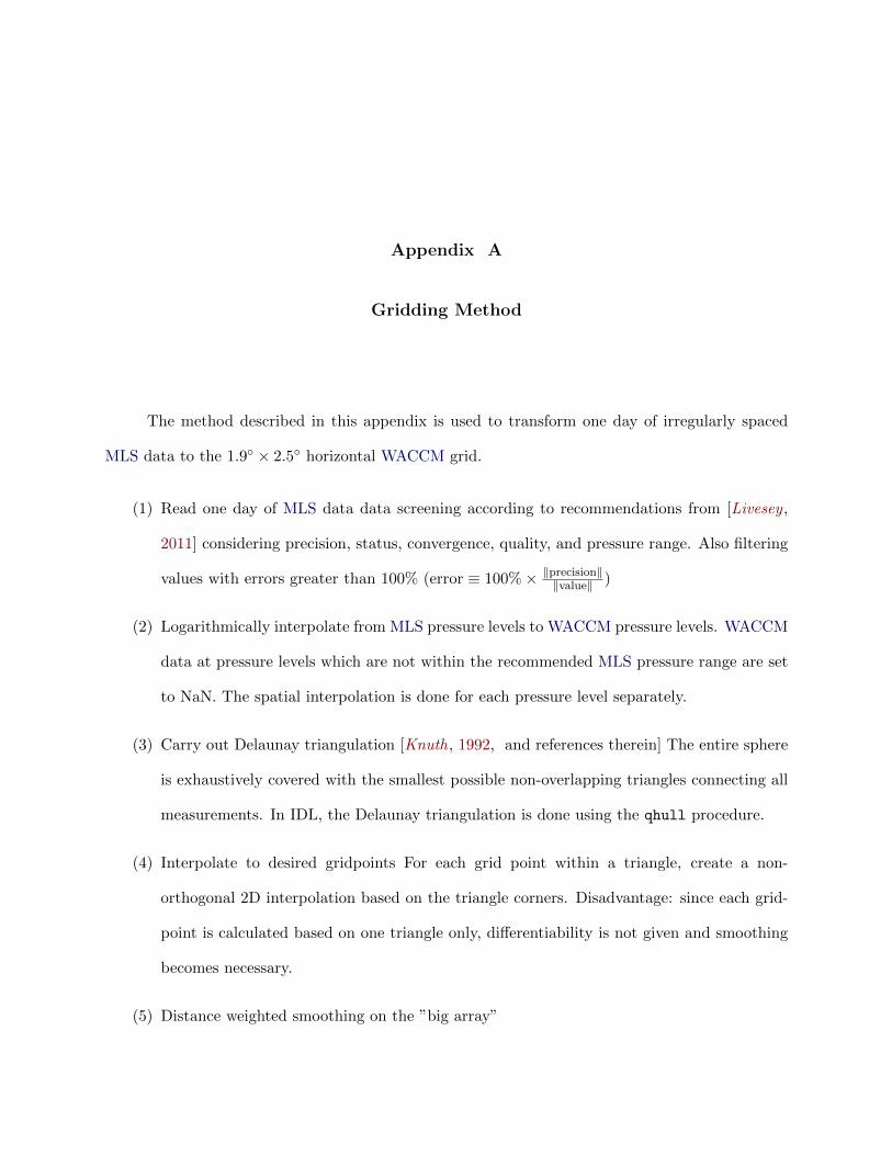
Appendix A
Gridding Method
The method described in this appendix is used to transform one day of irregularly spaced
MLS data to the 1.9◦ × 2.5◦ horizontal WACCM grid.
(1) Read one day of MLS data data screening according to recommendations from [Livesey ,
2011] considering precision, status, convergence, quality, and pressure range. Also filtering
values with errors greater than 100% (error ≡ 100%× ‖precision‖‖value‖ )
(2) Logarithmically interpolate from MLS pressure levels to WACCM pressure levels. WACCM
data at pressure levels which are not within the recommended MLS pressure range are set
to NaN. The spatial interpolation is done for each pressure level separately.
(3) Carry out Delaunay triangulation [Knuth, 1992, and references therein] The entire sphere
is exhaustively covered with the smallest possible non-overlapping triangles connecting all
measurements. In IDL, the Delaunay triangulation is done using the qhull procedure.
(4) Interpolate to desired gridpoints For each grid point within a triangle, create a non-
orthogonal 2D interpolation based on the triangle corners. Disadvantage: since each grid-
point is calculated based on one triangle only, differentiability is not given and smoothing
becomes necessary.
(5) Distance weighted smoothing on the ”big array”

(a) A ”big array” (Figure A.1) is an array combination of spatial geolocations that extends
the original spatial geolocations in all directions in order to avoid boundaries during
smoothing.
Figure A.1: Array combination in order to eliminate boundaries of the main data field (orange).Since the boundaries of the main data field are cyclic, copies of the main data field are appendedin ”zonal” direction (green) and in ”meridional” direction (blue) including a phase shift of 90◦W.For smoothing only the big array (red dashed) is used. After processing, the main array (orange)is extracted as the result.
(b) Create a kernel with the dimensions of 3 latitude gridpoints (which is a constant
length) and the equivalent length in longitudes (which is a length depending on lati-
tude).
(c) Fill the entire kernel with distance weights (e.g., inverse quadratic) around the center.
(d) Run convolution (smoothing) on red dashed field in Figure A.1: this removes artifacts
created by step 4.
(6) Save center array of the big array (orange field in Figure A.1) as the result.
124

Appendix B
Initialization Method
This appendix describes how the climatological initialization from WACCM is updated with
observations as described by Brakebusch et al. [2013].
(1) Choose date for initialization. For polar O3 loss investigations, the ideal initialization date
falls before the onset of O3 loss, but after the polar vortex is developed.
(2) Choose species to initialize. For initialization observations with representative polar cap
coverage are necessary. Initialization of species with diurnal variation is very difficult since
the observational coverage of one instrument at the time of initialization cannot cover the
entire polar cap. So for initialization of diurnally varying species, several instruments need
to be combined.
(3) Check availability of observations (global coverage within the day of initialization), find/create
initial condition model file from previous climatological run for subsequent initialization up-
date.
(4) Use gridding method to create distribution of profiles on WACCM grid (Appendix A)
(5) For each profile create a linear combination of observations and model: outside the valid
vertical range of the observations the linear combination consists of 100% climatological
data. Within the valid vertical range, the numbers of levels used for the transition depth
from 100% climatological data to 100% observation data back to 100% climatological data

depends on how similar the observations are to the model and how steep gradients are
at the transition regions. Figure B.1 shows the SD-WACCM, MLS, and initialization O3
profile on Dec 1, 2004 as used by Brakebusch et al. [2013]. Examples for this step can be
found in Table 3.1 in Chapter 3.
(6) Double check profiles if unphysical structure was introduced in the transition regions (e.g.,
local maxima). If necessary, adjust transition region depths.
(7) In the initial conditions file replace each species with the profiles just created (keep in mind
that the climatological initialization files from WACCM contain species in mass mixing
ratio and not volume mixing ratio).
Figure B.1: Example profile (Dec 1, 2004at 0◦E 90◦N) during initialization process:the original profile from the climatologicalWACCM initialization (blue), the observedprofile from MLS (red), and the updated ini-tialization profile (green). Here, O3 is takenfrom the climatological profile for pressure≥164 hPa, from MLS between 101-2.95 hPa,and from the climatological profile for pressure≤0.91 hPa.
126
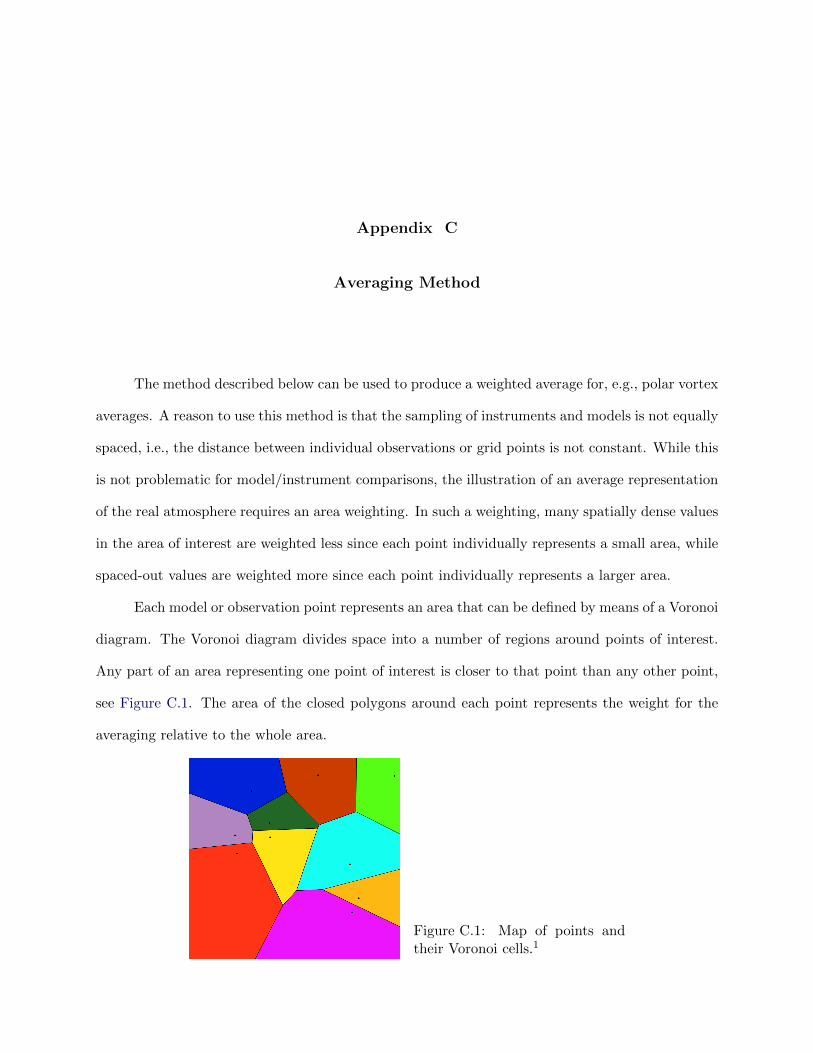
Appendix C
Averaging Method
The method described below can be used to produce a weighted average for, e.g., polar vortex
averages. A reason to use this method is that the sampling of instruments and models is not equally
spaced, i.e., the distance between individual observations or grid points is not constant. While this
is not problematic for model/instrument comparisons, the illustration of an average representation
of the real atmosphere requires an area weighting. In such a weighting, many spatially dense values
in the area of interest are weighted less since each point individually represents a small area, while
spaced-out values are weighted more since each point individually represents a larger area.
Each model or observation point represents an area that can be defined by means of a Voronoi
diagram. The Voronoi diagram divides space into a number of regions around points of interest.
Any part of an area representing one point of interest is closer to that point than any other point,
see Figure C.1. The area of the closed polygons around each point represents the weight for the
averaging relative to the whole area.
Figure C.1: Map of points andtheir Voronoi cells.1

When the appropriate averaging of a regular gridded model output (e.g., the standard 1.9◦×
2.5◦ WACCM grid) is of concern, a possible simplification is the multiplication of each grid point
with the cosine of its latitude since the meridional distance between each grid point is constant.
1 From http://commons.wikimedia.org/wiki/File:Voronoi diagram %2810 sites%29.svg, retrieved on2013/06/02.
128
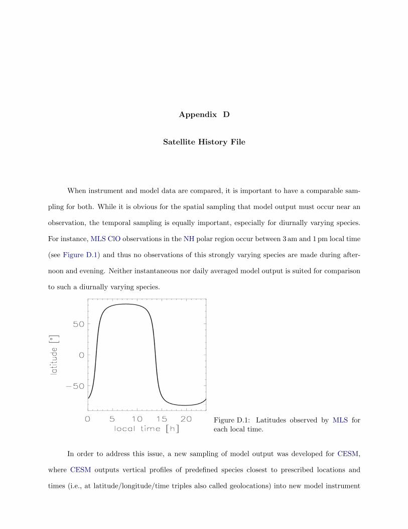
Appendix D
Satellite History File
When instrument and model data are compared, it is important to have a comparable sam-
pling for both. While it is obvious for the spatial sampling that model output must occur near an
observation, the temporal sampling is equally important, especially for diurnally varying species.
For instance, MLS ClO observations in the NH polar region occur between 3 am and 1 pm local time
(see Figure D.1) and thus no observations of this strongly varying species are made during after-
noon and evening. Neither instantaneous nor daily averaged model output is suited for comparison
to such a diurnally varying species.
Figure D.1: Latitudes observed by MLS foreach local time.
In order to address this issue, a new sampling of model output was developed for CESM,
where CESM outputs vertical profiles of predefined species closest to prescribed locations and
times (i.e., at latitude/longitude/time triples also called geolocations) into new model instrument

sampling output files. The resulting sampling error is less or equal to half the model grid size
and half the model time step. This form of sampled output comes at no significant increase in
computation time since the entire global field of each species is simulated at each time step anyway.
The list of geolocations provided to CESM is called satellite history file. This file contains
one-dimensional variables of at least latitude, longitude, and time from the observations of interest.
Any additional variable in the satellite history file, e.g., Julian day or SZA, is not considered for
model sampling but carried over into the sampled output files.
130

Appendix E
Workflow
Figure E.1: Workflow diagram for the work presented in Chapter 3, Chapter 4, and Chapter 5.Green boxes depict parts of the workflow that are provided by the scientific community, orangeboxes describe components of the workflow, and blue boxes indicate connections to the scientificcommunity.

List of Acronyms
ACE-FTS Atmospheric Chemistry Experiment Fourier
Transform Spectrometer
BDC Brewer Dobson circulation
CALIPSO Cloud-Aerosol Lidar and Infrared Pathfinder
Satellite Observation
CAM Community Atmosphere Model
CARMA Community Aerosol and Radiation Model
for Atmospheres
CCM chemistry climate model
CCMI Chemistry-Climate Model Initiative
CCMVal Chemistry-Climate Model Validation
CESM Community Earth System Model
CTM chemical transport model
DNA deoxyribonucleic acid
DU Dobson Units
EOS Earth Observing System
EP energetic particle
EPP energetic particle precipitation
ESM Earth System Model
ESMVal Earth System Model Validation
GEOS5 Goddard Earth Observing System 5
GHG greenhouse gas
GW gravity wave
IL inferred loss
IPCC Intergovernmental Panel on Climate Change
MEE medium energy electron
MERRA Modern-Era Retrospective analysis for
Research and Applications
MIPAS Michelson Interferometer for Passive
Atmospheric Sounding
ML modeled loss
MLS Microwave Limb Sounder
MOZART Model for OZone And Related chemical
Tracers
NASA National Aeronautics and Space
Administration
NCAR National Center for Atmospheric Research
NH northern hemisphere
NIR near infrared133
PNJ polar night jet
PSC polar stratospheric cloud
PV potential vorticity
PW planetary wave
SAD surface area density
SD-WACCM Specified Dynamics Whole Atmosphere
Community Climate Model
SH southern hemisphere
SLIMCAT SLIMCAT 3-D chemical transport model
SP solar proton
SPARC Stratospheric Processes And Their Role in
Climate
SPE solar proton event
sPV scaled potential vorticity
SSA stratospheric sulfate aerosol
SSW sudden stratospheric warming
STS supercooled ternary solution
SZA solar zenith angle
temperature temperature (T)
TIME-GCM Thermosphere-Ionosphere-Mesosphere
Electrodynamics General Circulation Model
UV ultra violet
134
VIS visible
VMR volume mixing ratio
VSL very short-lived
WACCM Whole Atmosphere Community Climate
Model
WMO World Meteorological Organization
135

List of Chemical Species
Br bromine
BrCl bromine chloride
BrO bromine monoxide
BrONO2 bromine nirate
BrOX reactive bromine
BrY inorganic bromine
CFC chlorofluorocarbon
CH3Br methyl bromide
CH3Cl methyl chloride
CH4 methane
Cl chlorine
Cl2 molecular chlorine
ClO chlorine monoxide
ClONO2 chlorine nirate
ClOOCl hypochlorite dimer (also Cl2O2)
ClOOCl hypochlorite dimer (also Cl2O2)
ClOX total reactive chlorine
ClY inorganic chlorine
CO carbon monoxide
CO2 carbon dioxide
COS carbonyl sulfide
F fluorine
H atomic hydrogen
H2O water vapor
HBr hydrogen bromide
HCl hydrogen chloride
HF hydrogen fluoride
HNO3 nitric acid
HNO4 peroxynitric acid
HO2 peroxyl radical
OH hydroxyl radical
HO2NO2 peroxinitric acid
HOBr hypobromous acid
HOCl hypochlorous acid
HOX odd hydrogen
HSO−3 hydrogen sulfite ion
I iodine
N2 molecular nitrogen
N2O nitrous oxide
N2O5 nitrogen pentoxide
NAT nitric acid trihydrate
NO nitrogen oxide137

NO2 nitrogen dioxide
NO3 nitrate radical
NOX nitrogen oxide, {NO+NO2}
NOY total reactive odd nitrogen {N + NO + NO2
+ NO3 + 2N2O5 + HO2NO2 + HNO3 +
ClONO2}
O atomic oxygen
O(1D) singlet D oxygen
O2 molecular oxygen
O3 ozone
O3TRAC ozone tracer
OClO chlorine dioxide
OX odd oxygen, {O+O3}
ppO3 pseudo-passive ozone
H2SO4 sulfuric acid
S sulfur
SO sulfur monoxide
sulfate sulfate ion, SO2−4
138


