Ensemble simulations of the decline and recovery of

stratospheric ozone

John Austin1 and R. John Wilson1

Received 24 November 2005; revised 27 March 2006; accepted 20 April 2006; published 30 August 2006.

[1] An ensemble of simulations of a coupled chemistry-climate model is completed for1960–2100. The simulations are divided into two periods, 1960–2005 and 1990–2100.The modeled total ozone amount decrease throughout the atmosphere from the 1960s untilabout 2000–2005, depending on latitude. The Antarctic ozone hole develops rapidly inthe model from about the late 1970s, in agreement with observations, but it does notdisappear until about 2065, about 15 years later than previous estimates. Spring averagedozone takes even longer to recover to 1980 values. Ozone amounts in the Antarctic aredetermined largely by halogen amounts. In contrast, in the Arctic, ozone recovers to 1980values about 25–35 years earlier, depending on the recovery criterion adopted. By the endof the 21st century, the climate change associated with greenhouse gas changes gives riseto a significant superrecovery of ozone in the Arctic but a less marked recovery in theAntarctic. For both polar regions, ensemble and interannual variability is greater in thefuture than in the past, and hence the timing of the full recovery of polar ozone is verysensitive to the definition of recovery. It is suggested that the range of recovery ratesbetween the hemispheres simulated in the model is related to the overall increase in thestrength of the Brewer-Dobson circulation, driven by increases in greenhouse gasconcentrations.

Citation: Austin, J., and R. J. Wilson (2006), Ensemble simulations of the decline and recovery of stratospheric ozone, J. Geophys.

Res., 111, D16314, doi:10.1029/2005JD006907.

1. Introduction

[2] The timing of future ozone recovery remains animportant topic [e.g., World Meteorological Organization(WMO)/United Nations Environment Programme (UNEP),2003; Newchurch et al., 2003; Steinbrecht et al., 2006; Yanget al., 2006; Miller et al., 2006], driven by scientificquestions such as: Will the Antarctic ozone hole recoverand if so when?, Is a similar hole likely to form over theArctic?, Will Arctic ozone decrease any further?, What arethe influences of ozone change on the troposphere?, Howis the Greenhouse effect influenced by future ozonerecovery? The questions have become increasingly sophis-ticated over the years and now demand the use of coupledchemistry-climate models for their answer. These modelshave all the problems associated with climate models suchas the need to have appropriate control runs and, to somedegree, the need to carry out ensemble simulations, toensure that model changes are a result of the changes inexternal parameters rather than internal model variability.[3] Many processes affect atmospheric ozone concentra-

tions. The direct chemical effect is via HOx, NOx, ClOx andBrOx reactions [e.g., Brasseur and Solomon, 1987]. Henceany process controlling the radical source molecules H2O,

N2O, chlorofuorocarbons (CFCs) and halons is important.Ozone chemistry is temperature-dependent, so changes inconcentrations of the well-mixed greenhouse gases (GHGs)are also significant, particularly CO2 in the stratosphere.Hereafter we refer to GHGs as implying just the well-mixedgreenhouse gases. Ozone itself and the source molecules aretransport-dependent and hence any process affecting trans-port and its future change [e.g., Butchart and Scaife, 2001;Butchart et al., 2006] is likely to play a role in slowing oraccelerating ozone depletion. Ozone is a radiatively activegas which tends to give rise to negative feedback. Forexample decreasing temperatures typically slows ozonecatalytic destruction cycles which increases ozone leadingto more solar heating. However, in the presence of polarstratospheric clouds (PSCs) reducing temperatures in thepresence of large halogen amounts leads to increased ozonedepletion [e.g. Austin et al., 1992]. There are also consid-erable uncertainties in the trends in water vapor [Randel etal., 2004] and models are typically unable to simulate thepast evolution in concentrations. As well as having animpact on ozone in the gas phase, via HOx catalyzeddestruction, the concentration of water vapor affects thedistribution of PSCs. It is perhaps not surprising that whenall these coupling processes have been included in models, awide range of results has been produced, particularly for thepolar regions where dynamical variability is large [WMO,2003, chapter 3; Austin et al., 2003].[4] In this work, results from a new model are presented

to address primarily the issue of ozone recovery. There are

JOURNAL OF GEOPHYSICAL RESEARCH, VOL. 111, D16314, doi:10.1029/2005JD006907, 2006ClickHere

for

FullArticle

1Geophysical Fluid Dynamics Laboratory, Princeton, New Jersey, USA.

Copyright 2006 by the American Geophysical Union.0148-0227/06/2005JD006907$09.00

D16314 1 of 16

many definitions of ozone recovery, concentrating forexample on the start of ozone recovery both using models[Austin et al., 2003] and observations [Newchurch et al.,2003; Reinsel et al., 2005; Yang et al., 2006; Miller etal., 2006]. A cautious approach [Weatherhead et al., 2000],takes recovery as being confirmed when a statisticallysignificant ozone increase has been observed. Their conclu-sion was that at least fifteen years of observations arerequired before the start of ozone recovery can be con-firmed. Caution concerning recovery has also beenexpressed by Steinbrecht et al. [2006], while Steinbrechtet al. [2004] point out the difficulty of identifying ozonerecovery in the context of solar variability.[5] In this work, we address ozone recovery from a

simpler point of view. The start of recovery is determinedas the date of ozone minimum in the time averaged resultsand the date of full recovery as the time averaged return to1980 total ozone amounts. Attributing ozone loss to halo-gens, built into some of the definitions of recovery, is hereconsidered important but different from the issue of recov-ery itself. Instead, 11-year running means are used to reducethe effects of the solar cycle and internal model variability.While some ozone depletion took place before 1980 [e.g.,

Solomon et al., 2005], as also shown in the model resultspresented here, it is a convenient definition of the start ofozone loss, as extensive stratospheric observations haveexisted only since the beginning of the satellite era.

2. Model Description and Simulations Completed

[6] The Geophysical Fluid Dynamics Laboratory (GFDL)Atmospheric Model with Transport and Chemistry (AM-TRAC), is described by Austin et al. [2006] and is acombination of the GFDL AM2 [Anderson et al., 2004]with chemistry from UMETRAC [Austin and Butchart,2003]. The AM2 has since been updated with finite volumeadvection and the chemistry has been improved principallyregarding the treatment of the long-lived tracers, as de-scribed in more detail by Austin et al. [2006]. The chemistrymodule is a comprehensive stratospheric scheme withsimplified tropospheric chemistry and is fully coupled tothe climate model. The photolysis rates are determined fromthe altitude, ozone column and solar zenith angle using aprecomputed look-up table. The table was constructed usingthe methods of Groves and Tuck [1980], but with updatedphotochemical data [Sander et al., 2003] in which the solarbeam is followed through the atmosphere, with explicitaccount taken of the geometry of the path length. Photolysisrates are calculated for solar zenith angles which exceed90�, but no allowance is made for refraction of the solarbeam.[7] The model resolution is 2� by 2.5� with 48 levels

from 0.0017 hPa to the ground. The vertical grid spacingdecreases steadily from the top of the atmosphere and in theupper stratosphere is about 4 km, decreasing to 1.5 km inthe lower stratosphere. The nonorographic gravity waveforcing scheme due to Alexander and Dunkerton [1999] isincluded in the model.[8] The model simulations are shown in Table 1. Both

time slice runs used sea surface temperatures and sea iceamounts (hereafter referred to jointly as SSTs) from a 1960to 2000 climatology. The GHG concentrations were set tothe values appropriate to the specific calendar year. A solar

Table 1. Brief Description of Model Simulations

Experiment Description Duration, years

SL1960 time slice 1960 conditions 30SL2000 time slice 2000 conditions 30TRANSA transient 1960–2005

initialized year 10 of SL196045

TRANSB transient 1960–2005initialized year 20 of SL1960

45

TRANSC transient 1960–2005initialized year 30 of SL1960

45

FUTURA transient 1990–2100initialized year 30 of TRANSA

110

FUTURB transient 1990–2100initialized year 30 of TRANSB

110

FUTURC transient 1990–2100initialized year 30 of TRANSC

110

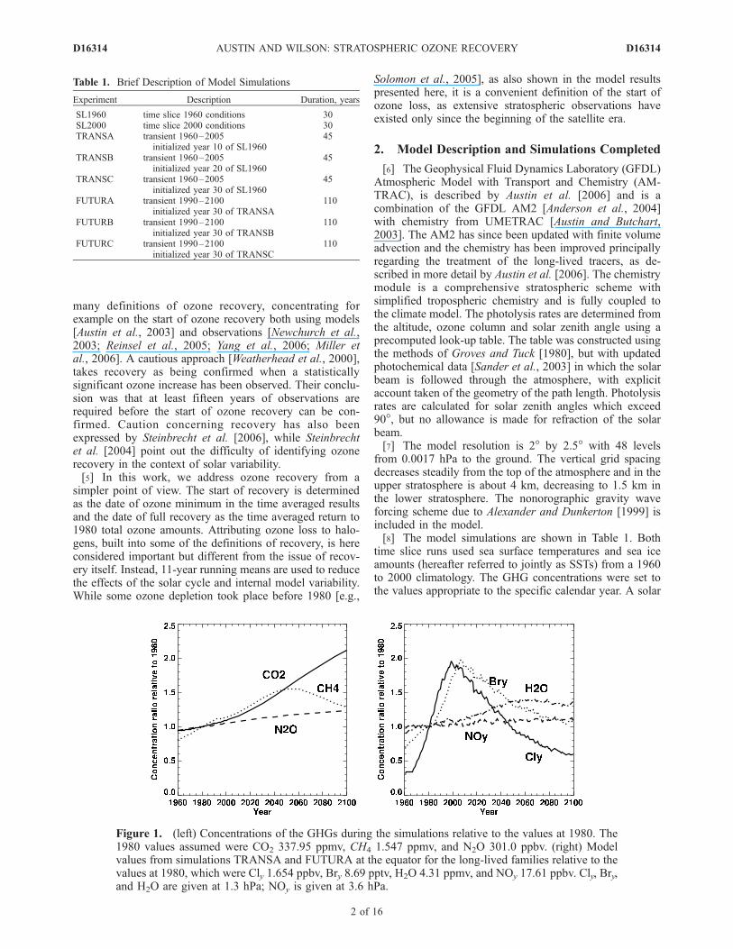
Figure 1. (left) Concentrations of the GHGs during the simulations relative to the values at 1980. The1980 values assumed were CO2 337.95 ppmv, CH4 1.547 ppmv, and N2O 301.0 ppbv. (right) Modelvalues from simulations TRANSA and FUTURA at the equator for the long-lived families relative to thevalues at 1980, which were Cly 1.654 ppbv, Bry 8.69 pptv, H2O 4.31 ppmv, and NOy 17.61 ppbv. Cly, Bry,and H2O are given at 1.3 hPa; NOy is given at 3.6 hPa.

D16314 AUSTIN AND WILSON: STRATOSPHERIC OZONE RECOVERY

2 of 16

D16314

cycle was not present in the forcing and aerosol amountswere set to background levels.[9] For the past runs, the model was forced with the same

time-dependent prescription of GHG and CFC concentra-tions, tropospheric and volcanic aerosols, and the solarcycle as from Delworth et al. [2006] and Knutson et al.

[2006]. Sea surface temperatures were obtained from theHurrell data set (J. Hurrell et al., personal communication,2005), extended to the beginning of the year 2005. For thefuture runs, the Intergovernmental Panel on Climate Change(IPCC) scenario A1B [IPCC, 2001, Appendix II] was usedfor the GHGs. The rate of change of active chlorine and

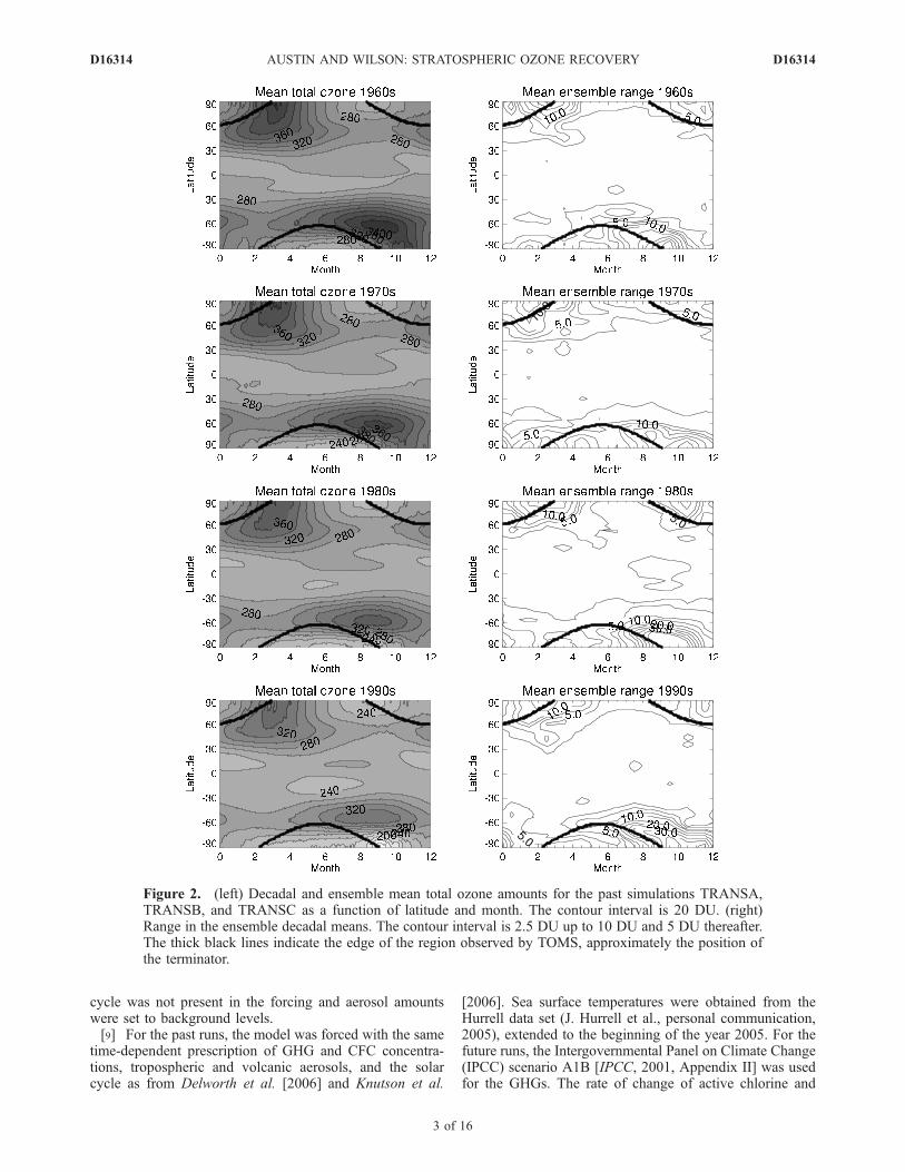
Figure 2. (left) Decadal and ensemble mean total ozone amounts for the past simulations TRANSA,TRANSB, and TRANSC as a function of latitude and month. The contour interval is 20 DU. (right)Range in the ensemble decadal means. The contour interval is 2.5 DU up to 10 DU and 5 DU thereafter.The thick black lines indicate the edge of the region observed by TOMS, approximately the position ofthe terminator.

D16314 AUSTIN AND WILSON: STRATOSPHERIC OZONE RECOVERY

3 of 16

D16314

bromine amounts in the model are computed using empir-ical functions of the destruction rates for each significantCFC and halon. CFC and halon concentrations were takenfrom WMO [2003, chapter 1, reference profile A1]. How-ever, because of model underprediction of age of air incomparison with measurements found in previous simula-tions of the model, it was found to be necessary to enhancethe effective destruction rates of the CFCs by 25% to obtainmore accurate Cly concentrations. The Bry values were notcorrected, since the age of air underprediction was foundnot to have a significant impact.[10] Volcanic aerosol amounts were taken as background

values and constant for the future. The optical depths wereaveraged from observations over the period 1996 to 1998and the results were smoothly joined to the data from 1997onward. This results in higher aerosol values than observedfor the period 1997 to 2005. At these concentrations, theinfluence of aerosol changes on the results is small but,arguably, the values are more representative of a postvolcanic atmosphere over the long term than, for example,the current very clean stratosphere. Sea surface temperaturesand sea ice amounts were taken from a coupled atmosphere-ocean model simulation of the same core climate model, butwith fewer vertical levels (simulation CM2.1 of Delworth etal. [2006]). A solar cycle was maintained into the future byrepeating the last 5 cycles for which detailed observations of10.7 cm radio flux are available.[11] The past runs were initialized from years 10, 20 and

30 of the 1960 time slice run. Unfortunately, because ofdifferent aerosol amounts and difference in the amount of

solar forcing, the past runs still needed a few years to spinup to their balanced state. The future runs were initializedfrom 1 January 1990 of the corresponding past run. Afifteen year overlap between the past and future runs was setup to test the impact of the switch in sea surface temper-atures from observation to model results. In most cases thishad no impact on the model results.

3. Greenhouse Gas Concentrations andLong-Lived Species

[12] The main long-lived species which affect ozone areshown in Figure 1. In Figure 1 (left) are shown the GHGsfor the troposphere, which were specified. In Figure 1(right), values are shown for long-lived chemical speciescomputed by the model near the equatorial stratopause. Allthe values have been scaled to the values for 1980 (seeFigure 1 caption for details). The CO2 and N2O amounts aretaken to increase steadily. Methane amounts are taken toincrease in the early part of the integration and are taken todecrease from about 2050. The methane amounts, togetherwith changes in the tropical tropopause temperature, giverise to the changes in water vapor amounts shown inFigure 1 (right). By 2060, water vapor amounts hadincreased by about 40% but did not decrease substantiallyin the final few decades despite lowering methane amounts.[13] The Cly and Bry concentrations at 1.3 hPa at

the equator are shown in Figure 1 (right) throughout the140-year simulation period. At this location, modeled Clypeaked at 3.3 ppbv in 1997 and Bry peaked at 17.2 pptv in2007. Return to 1980 values is projected to occur by about

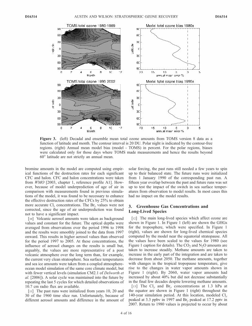
Figure 3. (left) Decadal and ensemble mean total ozone amounts from TOMS version 8 data as afunction of latitude and month. The contour interval is 20 DU. Polar night is indicated by the contour-freeregions. (right) Annual mean model bias (model - TOMS) in percent. For the polar regions, biaseswere calculated only for those days where TOMS made measurements and hence the results beyond60� latitude are not strictly an annual mean.

D16314 AUSTIN AND WILSON: STRATOSPHERIC OZONE RECOVERY

4 of 16

D16314

2050 for Cly but not before the end of the simulations forBry. The amount of NOy at 3.6 hPa at the equator, near themodel peak, increased only slightly during the simulations.

4. Past Simulations of Ozone

4.1. Decadal Variation in Total Ozone

[14] Figure 2 (left) shows the decadal averages of simu-lated total ozone averaged over all three ensemble members.Tropical ozone decreased throughout the period from about260 DU in the 1960s to below 240 DU by the 1990s. In theNorthern Hemisphere, maximum ozone occurred over theNorth Pole in spring time with a distinct minimum overthe Arctic during autumn. In the Southern Hemisphere, peakozone values occurred in middle to high latitudes, with theAntarctic ozone hole occurring in the 1980s and 1990s.Ozone decreased everywhere during the simulations.[15] Figure 2 (right) shows the range in the ensemble

members. Data from each of the simulations was averagedover decade and over days in the month before calculatingthe range. There was considerable daily variability necessi-tating the monthly averaging before calculating the range in

order to observe a clear signal. In the tropics and subtropics,the ensemble range is small, typically less than 2.5 DU. Therange is much larger in the polar regions and exceeds 30DUover the South Pole in the later decades. This demonstratesthe well-known behavior [e.g., WMO, 2003, chapter 3] thatlargest atmospheric variability and uncertainty occurs in thepolar regions.[16] Decadal averages from Total Ozone Mapping Spec-

trometer (TOMS) version 8 data [Wellemeyer et al., 2004;P. K. Bhartia and C. G. Wellemeyer, TOMS-V8 total O3algorithm, available at http://toms.gsfc.nasa.gov/version8/version8_update.html, document toms_atbd.pdf, 2005) andmodel biases are shown in Figure 3. The TOMS data,nominally for the 1990s, here includes also the years2000–2002 to compensate for the gaps in data coverageduring 1993 to 1996. The model seasonal variations(Figure 2) are in good agreement with TOMS, and hence,for clarity, Figure 3 (right) shows only the annual meanmodelbias. For both decades, the latitudinal variation of the bias isvery similar but with larger biases in the 1990s. In theSouthern Hemisphere, the results are in good agreement withobservations in both decades, with biases typically about 5%

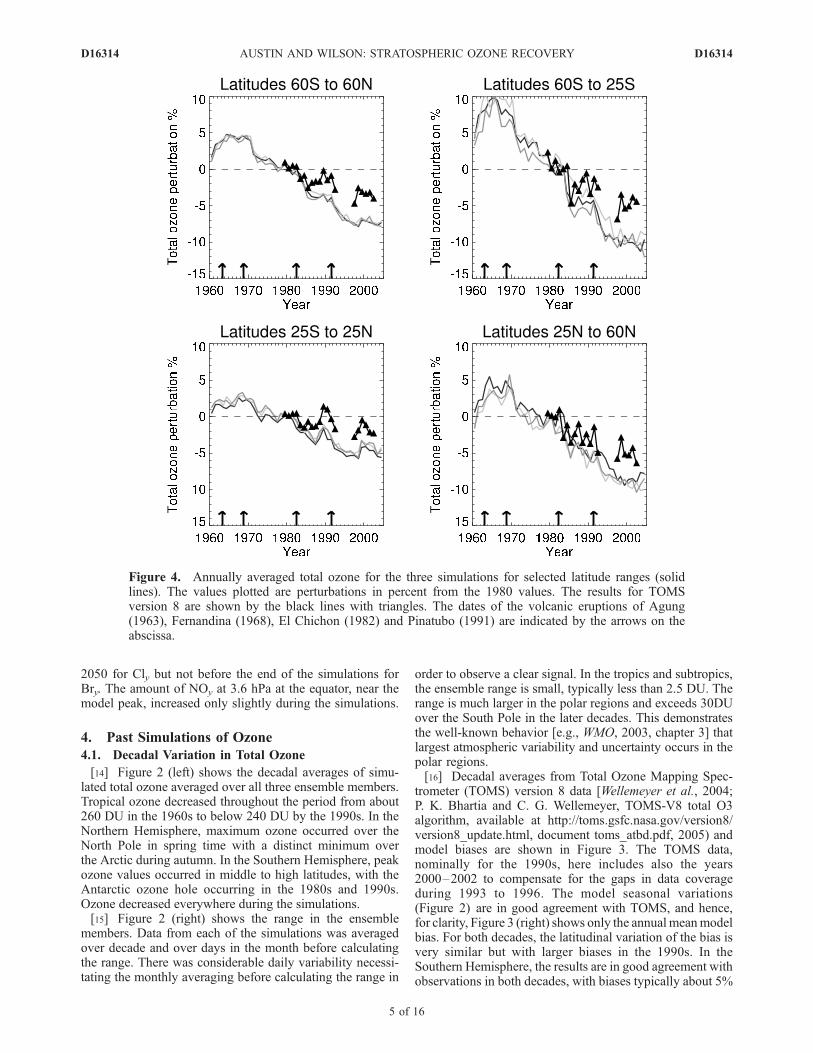
Figure 4. Annually averaged total ozone for the three simulations for selected latitude ranges (solidlines). The values plotted are perturbations in percent from the 1980 values. The results for TOMSversion 8 are shown by the black lines with triangles. The dates of the volcanic eruptions of Agung(1963), Fernandina (1968), El Chichon (1982) and Pinatubo (1991) are indicated by the arrows on theabscissa.

D16314 AUSTIN AND WILSON: STRATOSPHERIC OZONE RECOVERY

5 of 16

D16314

in magnitude. The model’s low bias increases steadily withlatitude toward the North Pole, where it reaches about 15%.

4.2. Regionally Averaged Total Ozone

[17] Area averaged ozone for tropical and midlatitudes isshown in Figure 4 in comparison with TOMS version 8 data.TOMS (version 7) and ground-based data show similartrends [Fioletov et al., 2002]. Over the period 1980–2000, the general pattern of the observations was repro-duced, but the simulated ozone decreased by about 2% perdecade globally relative to the observations. The impact ofthe eruptions of El Chichon and Mount Pinatubo areparticularly apparent in the observed tropical values, result-ing in a decrease of about 2% for El Chichon (May 1982)and more than 3% for Mount Pinatubo (June 1991), relativeto the preeruption date. The model reproduced these fea-tures, but they are partially obscured by the overall modeltrend. During the eruption of Agung (March 1963) andFernandina (November 1968), model ozone values in-creased in accordance with the study of Tie and Brasseur

[1995]. During the 1960s the impact of the heterogeneousreactions on the volcanic aerosol was to convert N2O5 toHNO3 which reduces catalytic ozone destruction by NOx.This mechanism is later superseded by halogen effects forwhich catalytic ozone destruction is increased by heteroge-neous reactions. In comparison, Dameris et al. [2005] andC. Bruhl et al. (personal communication, 2005), obtainresults which agree better with observations for the recentpast, and show a smaller ozone increase from the Agungeruption. In that case the stratospheric temperature increasefollowing the eruption was much larger than in AMTRACand any reduction in NOx catalyzed destruction was coun-terbalanced by increased HOx catalyzed destruction.[18] Ozone trends were computed for the period 1980 to

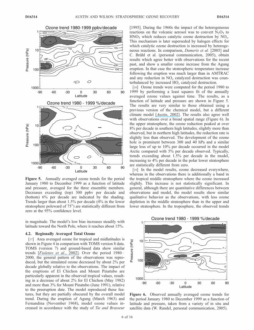
1999 by performing a least squares fit of the annuallyaveraged ozone values against time. The results, as afunction of latitude and pressure are shown in Figure 5.The results are very similar to those obtained using aprevious version of the chemical model, but a differentclimate model [Austin, 2002]. The results also agree wellwith observations over a broad spatial range (Figure 6). Inthe upper stratosphere, the ozone reduction peaked at over8% per decade in southern high latitudes, slightly more thanobserved, but in northern high latitudes, the reduction rate isslightly less than observed. The development of the ozonehole is prominent between 300 and 40 hPa and a similarlarge loss of up to 10% per decade occurred in the modelArctic compared with 5% per decade observed. Typically,trends exceeding about 1.5% per decade in the model,increasing to 4% per decade in the polar lower stratosphereare statistically different from zero.[19] In the model results, ozone decreased everywhere,

whereas in the observations there is additionally a band inthe tropical middle stratosphere where the ozone increasedslightly. This increase is not statistically significant. Ingeneral, although there are quantitative differences betweenobservations and model, the model results show similarqualitative behavior as the observations, with less ozonedepletion in the middle stratosphere than in the upper andlower stratosphere. In the troposphere, the observed trends

Figure 5. Annually averaged ozone trends for the periodJanuary 1980 to December 1999 as a function of latitudeand pressure, averaged for the three ensemble members.Decreases exceeding (top) 300 ppbv per decade and(bottom) 6% per decade are indicated by the shading.Trends larger than about 1.5% per decade (4% in the lowerstratosphere poleward of 75�) are statistically different fromzero at the 95% confidence level.

Figure 6. Observed annually averaged ozone trends forthe period January 1980 to December 1999 as a function oflatitude and pressure, taken from a variety of in situ andsatellite data (W. Randel, personal communication, 2005).

D16314 AUSTIN AND WILSON: STRATOSPHERIC OZONE RECOVERY

6 of 16

D16314

are not significantly different from zero, but simulatedozone decreased by several percent per decade. In the modelthe results are influenced by downward transport from theozone hole and increased HOx depletion arising fromincreased water vapor. The former could be due to numer-ical mixing, arising from the limited resolution in thevicinity of the tropopause. Increases in NOx would increaseozone in the troposphere and correct the model error, but inthe model simulations NOx has been kept constant there.

4.3. Vertical Profiles of Ozone

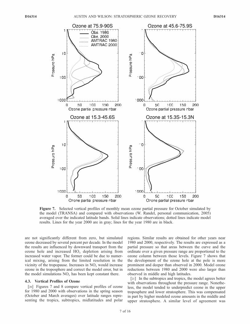
[20] Figures 7 and 8 compare vertical profiles of ozonefor 1980 and 2000 with observations in the spring season(October and March averages) over latitude ranges repre-senting the tropics, subtropics, midlatitudes and polar

regions. Similar results are obtained for other years near1980 and 2000, respectively. The results are expressed as apartial pressure so that areas between the curve and theordinate over a given pressure range are proportional to theozone column between those levels. Figure 7 shows thatthe development of the ozone hole at the pole is moreprominent and deeper than observed in 2000. Model ozonereductions between 1980 and 2000 were also larger thanobserved in middle and high latitudes.[21] In the subtropics and tropics, the model agrees better

with observations throughout the pressure range. Nonethe-less, the model tended to underpredict ozone in the uppertroposphere and lower stratosphere. This was compensatedin part by higher modeled ozone amounts in the middle andupper stratosphere. A similar level of agreement was

Figure 7. Selected vertical profiles of monthly mean ozone partial pressure for October simulated bythe model (TRANSA) and compared with observations (W. Randel, personal communication, 2005)averaged over the indicated latitude bands. Solid lines indicate observations; dotted lines indicate modelresults. Lines for the year 2000 are in gray; lines for the year 1980 are in black.

D16314 AUSTIN AND WILSON: STRATOSPHERIC OZONE RECOVERY

7 of 16

D16314

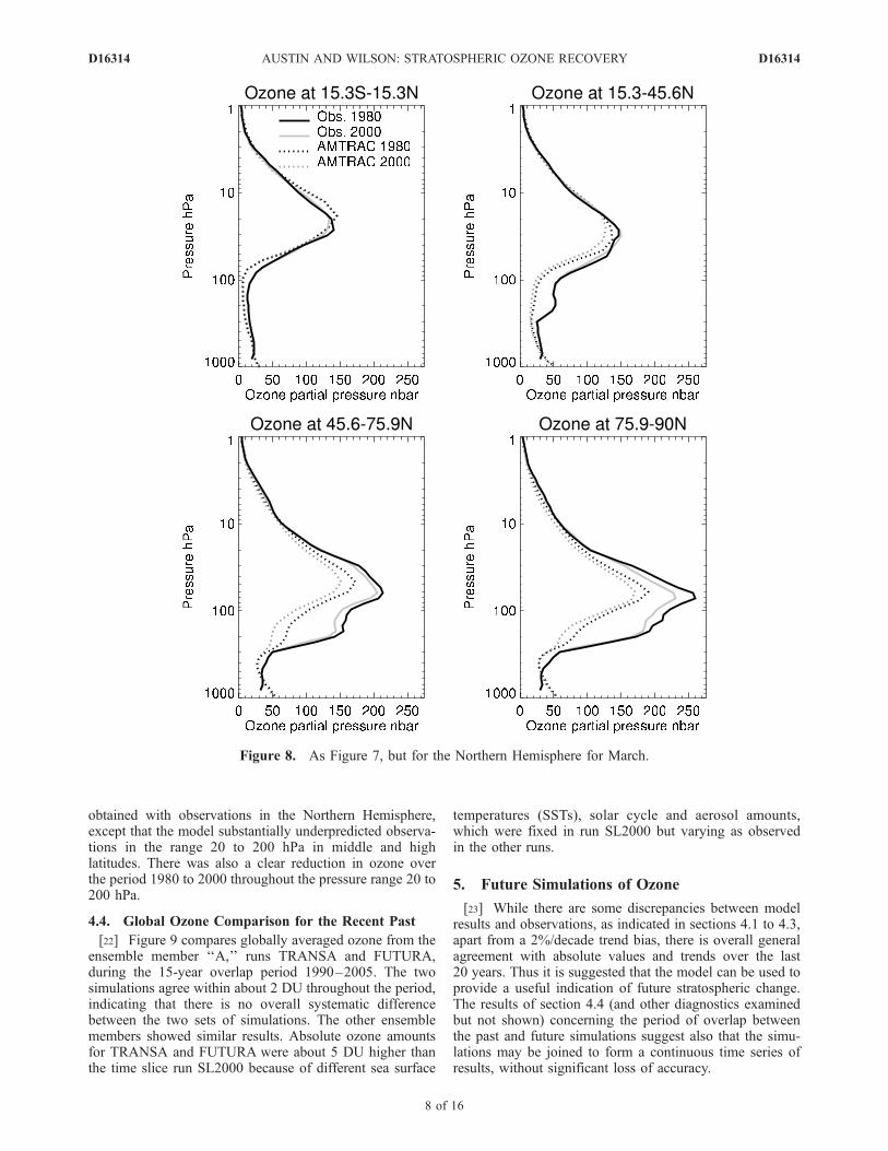
obtained with observations in the Northern Hemisphere,except that the model substantially underpredicted observa-tions in the range 20 to 200 hPa in middle and highlatitudes. There was also a clear reduction in ozone overthe period 1980 to 2000 throughout the pressure range 20 to200 hPa.

4.4. Global Ozone Comparison for the Recent Past

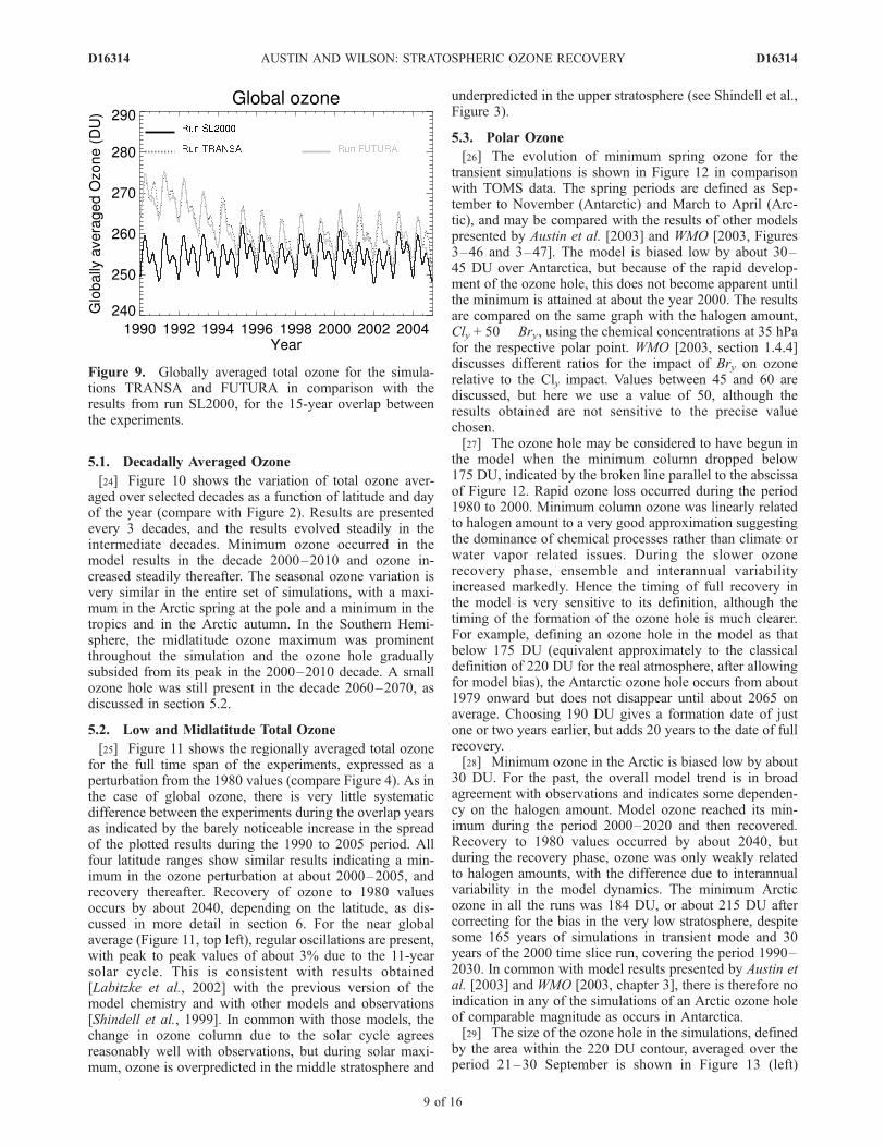
[22] Figure 9 compares globally averaged ozone from theensemble member ‘‘A,’’ runs TRANSA and FUTURA,during the 15-year overlap period 1990–2005. The twosimulations agree within about 2 DU throughout the period,indicating that there is no overall systematic differencebetween the two sets of simulations. The other ensemblemembers showed similar results. Absolute ozone amountsfor TRANSA and FUTURA were about 5 DU higher thanthe time slice run SL2000 because of different sea surface

temperatures (SSTs), solar cycle and aerosol amounts,which were fixed in run SL2000 but varying as observedin the other runs.

5. Future Simulations of Ozone

[23] While there are some discrepancies between modelresults and observations, as indicated in sections 4.1 to 4.3,apart from a 2%/decade trend bias, there is overall generalagreement with absolute values and trends over the last20 years. Thus it is suggested that the model can be used toprovide a useful indication of future stratospheric change.The results of section 4.4 (and other diagnostics examinedbut not shown) concerning the period of overlap betweenthe past and future simulations suggest also that the simu-lations may be joined to form a continuous time series ofresults, without significant loss of accuracy.

Figure 8. As Figure 7, but for the Northern Hemisphere for March.

D16314 AUSTIN AND WILSON: STRATOSPHERIC OZONE RECOVERY

8 of 16

D16314

5.1. Decadally Averaged Ozone

[24] Figure 10 shows the variation of total ozone aver-aged over selected decades as a function of latitude and dayof the year (compare with Figure 2). Results are presentedevery 3 decades, and the results evolved steadily in theintermediate decades. Minimum ozone occurred in themodel results in the decade 2000–2010 and ozone in-creased steadily thereafter. The seasonal ozone variation isvery similar in the entire set of simulations, with a maxi-mum in the Arctic spring at the pole and a minimum in thetropics and in the Arctic autumn. In the Southern Hemi-sphere, the midlatitude ozone maximum was prominentthroughout the simulation and the ozone hole graduallysubsided from its peak in the 2000–2010 decade. A smallozone hole was still present in the decade 2060–2070, asdiscussed in section 5.2.

5.2. Low and Midlatitude Total Ozone

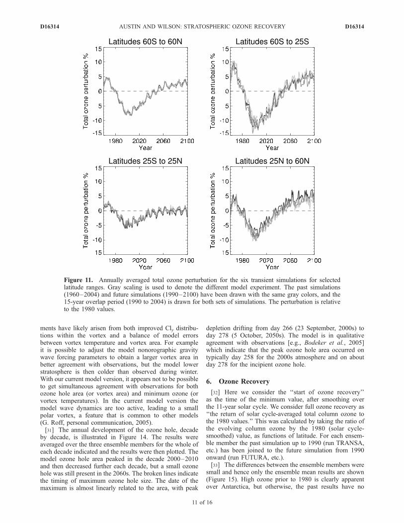
[25] Figure 11 shows the regionally averaged total ozonefor the full time span of the experiments, expressed as aperturbation from the 1980 values (compare Figure 4). As inthe case of global ozone, there is very little systematicdifference between the experiments during the overlap yearsas indicated by the barely noticeable increase in the spreadof the plotted results during the 1990 to 2005 period. Allfour latitude ranges show similar results indicating a min-imum in the ozone perturbation at about 2000–2005, andrecovery thereafter. Recovery of ozone to 1980 valuesoccurs by about 2040, depending on the latitude, as dis-cussed in more detail in section 6. For the near globalaverage (Figure 11, top left), regular oscillations are present,with peak to peak values of about 3% due to the 11-yearsolar cycle. This is consistent with results obtained[Labitzke et al., 2002] with the previous version of themodel chemistry and with other models and observations[Shindell et al., 1999]. In common with those models, thechange in ozone column due to the solar cycle agreesreasonably well with observations, but during solar maxi-mum, ozone is overpredicted in the middle stratosphere and

underpredicted in the upper stratosphere (see Shindell et al.,Figure 3).

5.3. Polar Ozone

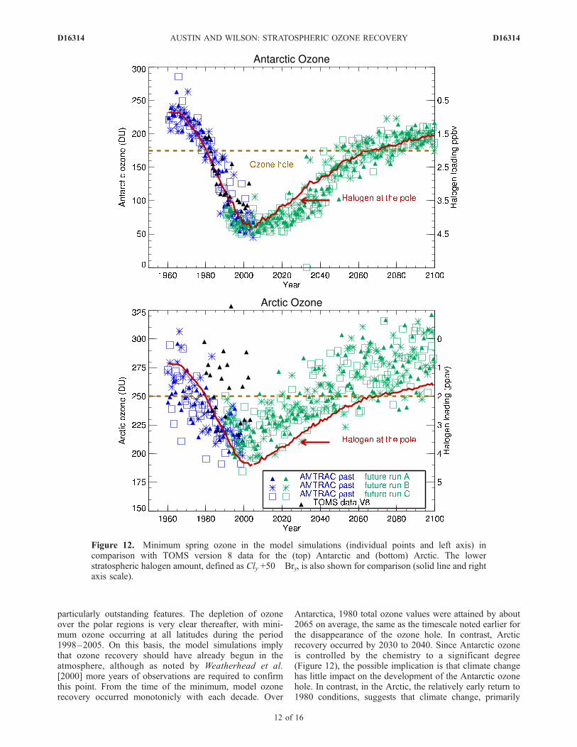
[26] The evolution of minimum spring ozone for thetransient simulations is shown in Figure 12 in comparisonwith TOMS data. The spring periods are defined as Sep-tember to November (Antarctic) and March to April (Arc-tic), and may be compared with the results of other modelspresented by Austin et al. [2003] and WMO [2003, Figures3–46 and 3–47]. The model is biased low by about 30–45 DU over Antarctica, but because of the rapid develop-ment of the ozone hole, this does not become apparent untilthe minimum is attained at about the year 2000. The resultsare compared on the same graph with the halogen amount,Cly + 50 � Bry, using the chemical concentrations at 35 hPafor the respective polar point. WMO [2003, section 1.4.4]discusses different ratios for the impact of Bry on ozonerelative to the Cly impact. Values between 45 and 60 arediscussed, but here we use a value of 50, although theresults obtained are not sensitive to the precise valuechosen.[27] The ozone hole may be considered to have begun in

the model when the minimum column dropped below175 DU, indicated by the broken line parallel to the abscissaof Figure 12. Rapid ozone loss occurred during the period1980 to 2000. Minimum column ozone was linearly relatedto halogen amount to a very good approximation suggestingthe dominance of chemical processes rather than climate orwater vapor related issues. During the slower ozonerecovery phase, ensemble and interannual variabilityincreased markedly. Hence the timing of full recovery inthe model is very sensitive to its definition, although thetiming of the formation of the ozone hole is much clearer.For example, defining an ozone hole in the model as thatbelow 175 DU (equivalent approximately to the classicaldefinition of 220 DU for the real atmosphere, after allowingfor model bias), the Antarctic ozone hole occurs from about1979 onward but does not disappear until about 2065 onaverage. Choosing 190 DU gives a formation date of justone or two years earlier, but adds 20 years to the date of fullrecovery.[28] Minimum ozone in the Arctic is biased low by about

30 DU. For the past, the overall model trend is in broadagreement with observations and indicates some dependen-cy on the halogen amount. Model ozone reached its min-imum during the period 2000–2020 and then recovered.Recovery to 1980 values occurred by about 2040, butduring the recovery phase, ozone was only weakly relatedto halogen amounts, with the difference due to interannualvariability in the model dynamics. The minimum Arcticozone in all the runs was 184 DU, or about 215 DU aftercorrecting for the bias in the very low stratosphere, despitesome 165 years of simulations in transient mode and 30years of the 2000 time slice run, covering the period 1990–2030. In common with model results presented by Austin etal. [2003] and WMO [2003, chapter 3], there is therefore noindication in any of the simulations of an Arctic ozone holeof comparable magnitude as occurs in Antarctica.[29] The size of the ozone hole in the simulations, defined

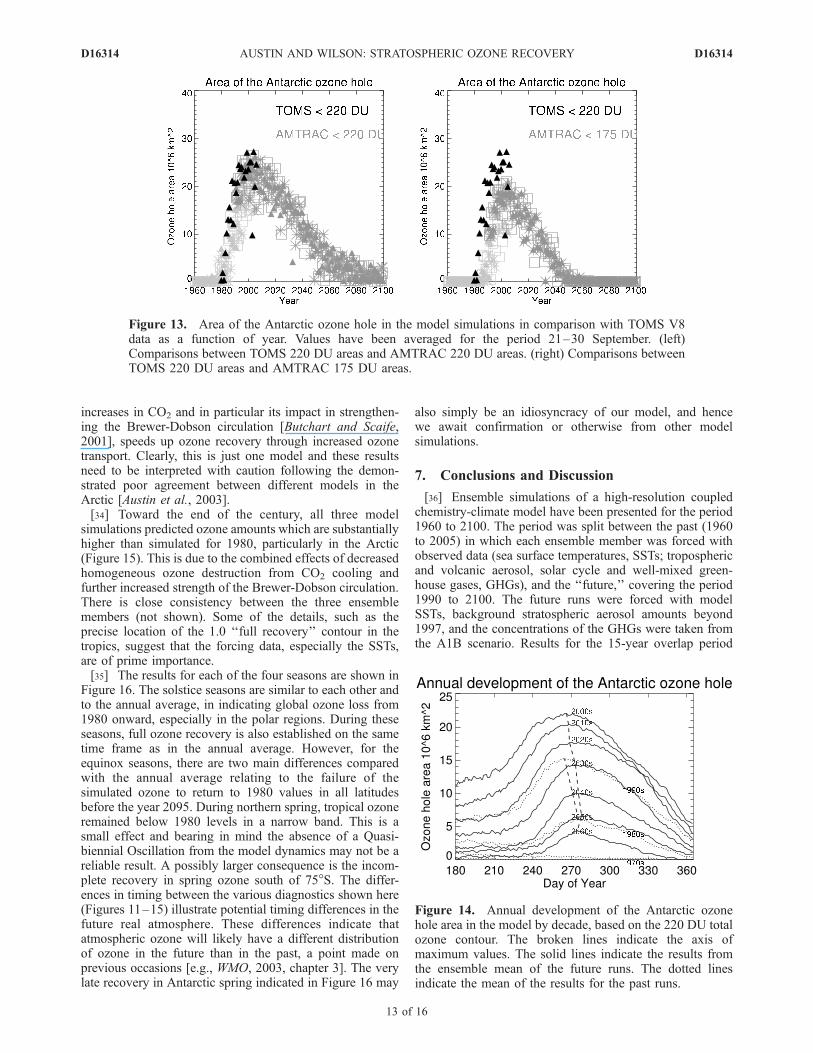
by the area within the 220 DU contour, averaged over theperiod 21–30 September is shown in Figure 13 (left)

Figure 9. Globally averaged total ozone for the simula-tions TRANSA and FUTURA in comparison with theresults from run SL2000, for the 15-year overlap betweenthe experiments.

D16314 AUSTIN AND WILSON: STRATOSPHERIC OZONE RECOVERY

9 of 16

D16314

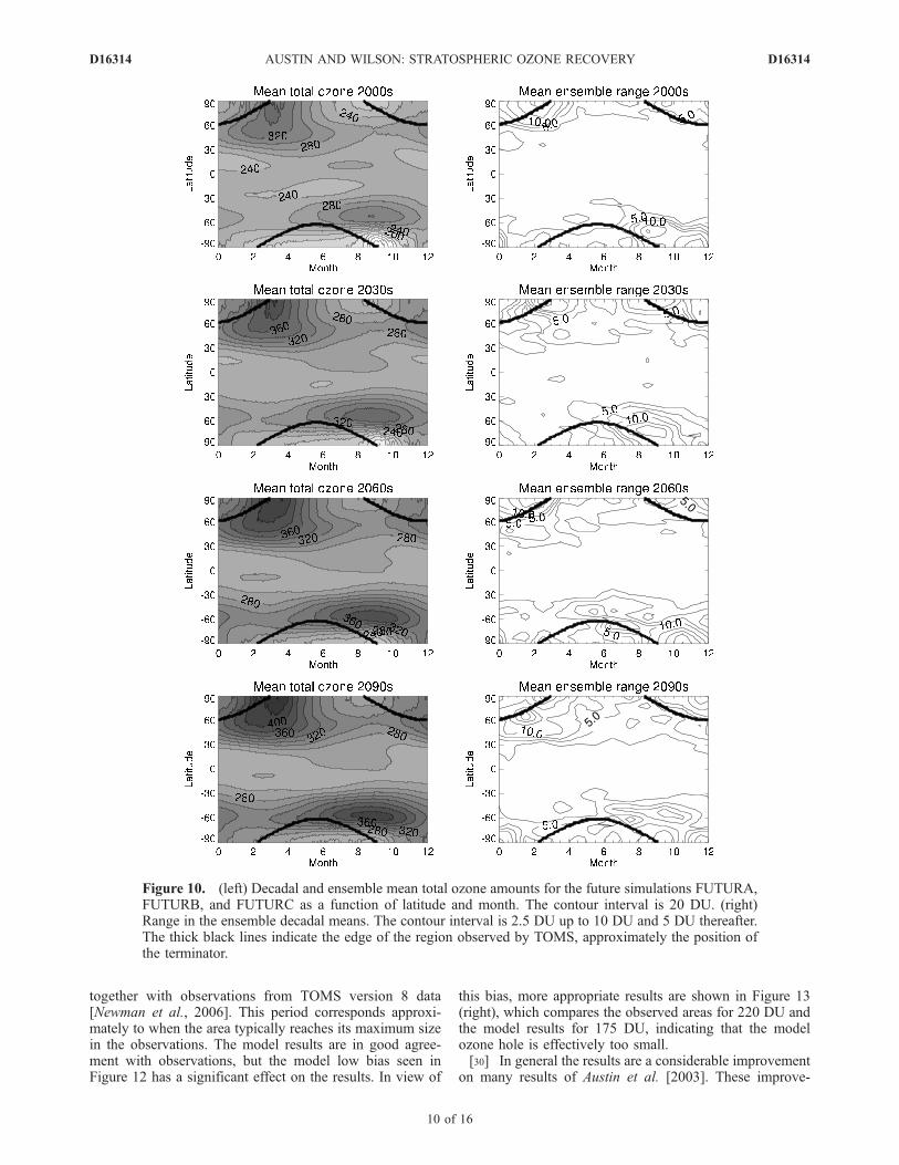
together with observations from TOMS version 8 data[Newman et al., 2006]. This period corresponds approxi-mately to when the area typically reaches its maximum sizein the observations. The model results are in good agree-ment with observations, but the model low bias seen inFigure 12 has a significant effect on the results. In view of

this bias, more appropriate results are shown in Figure 13(right), which compares the observed areas for 220 DU andthe model results for 175 DU, indicating that the modelozone hole is effectively too small.[30] In general the results are a considerable improvement

on many results of Austin et al. [2003]. These improve-

Figure 10. (left) Decadal and ensemble mean total ozone amounts for the future simulations FUTURA,FUTURB, and FUTURC as a function of latitude and month. The contour interval is 20 DU. (right)Range in the ensemble decadal means. The contour interval is 2.5 DU up to 10 DU and 5 DU thereafter.The thick black lines indicate the edge of the region observed by TOMS, approximately the position ofthe terminator.

D16314 AUSTIN AND WILSON: STRATOSPHERIC OZONE RECOVERY

10 of 16

D16314

ments have likely arisen from both improved Cly distribu-tions within the vortex and a balance of model errorsbetween vortex temperature and vortex area. For exampleit is possible to adjust the model nonorographic gravitywave forcing parameters to obtain a larger vortex area inbetter agreement with observations, but the model lowerstratosphere is then colder than observed during winter.With our current model version, it appears not to be possibleto get simultaneous agreement with observations for bothozone hole area (or vortex area) and minimum ozone (orvortex temperatures). In the current model version themodel wave dynamics are too active, leading to a smallpolar vortex, a feature that is common to other models(G. Roff, personal communication, 2005).[31] The annual development of the ozone hole, decade

by decade, is illustrated in Figure 14. The results wereaveraged over the three ensemble members for the whole ofeach decade indicated and the results were then plotted. Themodel ozone hole area peaked in the decade 2000–2010and then decreased further each decade, but a small ozonehole was still present in the 2060s. The broken lines indicatethe timing of maximum ozone hole size. The date of themaximum is almost linearly related to the area, with peak

depletion drifting from day 266 (23 September, 2000s) today 278 (5 October, 2050s). The model is in qualitativeagreement with observations [e.g., Bodeker et al., 2005]which indicate that the peak ozone hole area occurred ontypically day 258 for the 2000s atmosphere and on aboutday 278 for the incipient ozone hole.

6. Ozone Recovery

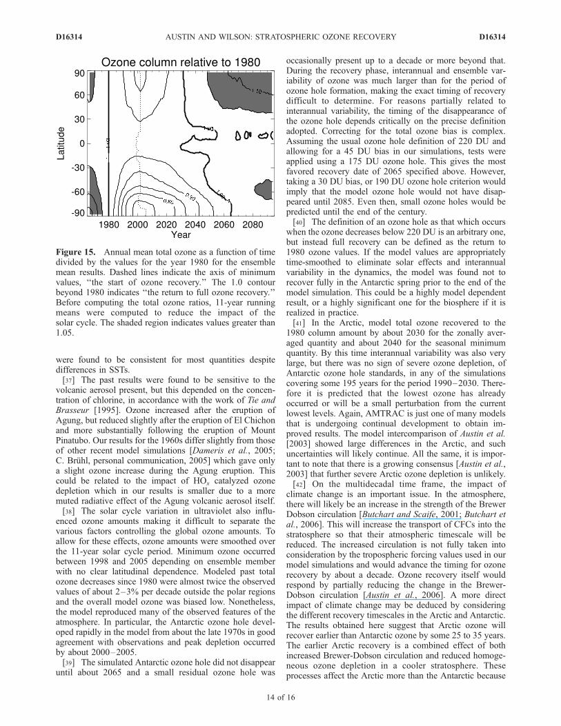
[32] Here we consider the ‘‘start of ozone recovery’’as the time of the minimum value, after smoothing overthe 11-year solar cycle. We consider full ozone recovery as‘‘the return of solar cycle-averaged total column ozone tothe 1980 values.’’ This was calculated by taking the ratio ofthe evolving column ozone by the 1980 (solar cycle-smoothed) value, as functions of latitude. For each ensem-ble member the past simulation up to 1990 (run TRANSA,etc.) has been joined to the future simulation from 1990onward (run FUTURA, etc.).[33] The differences between the ensemble members were

small and hence only the ensemble mean results are shown(Figure 15). High ozone prior to 1980 is clearly apparentover Antarctica, but otherwise, the past results have no

Figure 11. Annually averaged total ozone perturbation for the six transient simulations for selectedlatitude ranges. Gray scaling is used to denote the different model experiment. The past simulations(1960–2004) and future simulations (1990–2100) have been drawn with the same gray colors, and the15-year overlap period (1990 to 2004) is drawn for both sets of simulations. The perturbation is relativeto the 1980 values.

D16314 AUSTIN AND WILSON: STRATOSPHERIC OZONE RECOVERY

11 of 16

D16314

particularly outstanding features. The depletion of ozoneover the polar regions is very clear thereafter, with mini-mum ozone occurring at all latitudes during the period1998–2005. On this basis, the model simulations implythat ozone recovery should have already begun in theatmosphere, although as noted by Weatherhead et al.[2000] more years of observations are required to confirmthis point. From the time of the minimum, model ozonerecovery occurred monotonicly with each decade. Over

Antarctica, 1980 total ozone values were attained by about2065 on average, the same as the timescale noted earlier forthe disappearance of the ozone hole. In contrast, Arcticrecovery occurred by 2030 to 2040. Since Antarctic ozoneis controlled by the chemistry to a significant degree(Figure 12), the possible implication is that climate changehas little impact on the development of the Antarctic ozonehole. In contrast, in the Arctic, the relatively early return to1980 conditions, suggests that climate change, primarily

Figure 12. Minimum spring ozone in the model simulations (individual points and left axis) incomparison with TOMS version 8 data for the (top) Antarctic and (bottom) Arctic. The lowerstratospheric halogen amount, defined as Cly +50� Bry, is also shown for comparison (solid line and rightaxis scale).

D16314 AUSTIN AND WILSON: STRATOSPHERIC OZONE RECOVERY

12 of 16

D16314

increases in CO2 and in particular its impact in strengthen-ing the Brewer-Dobson circulation [Butchart and Scaife,2001], speeds up ozone recovery through increased ozonetransport. Clearly, this is just one model and these resultsneed to be interpreted with caution following the demon-strated poor agreement between different models in theArctic [Austin et al., 2003].[34] Toward the end of the century, all three model

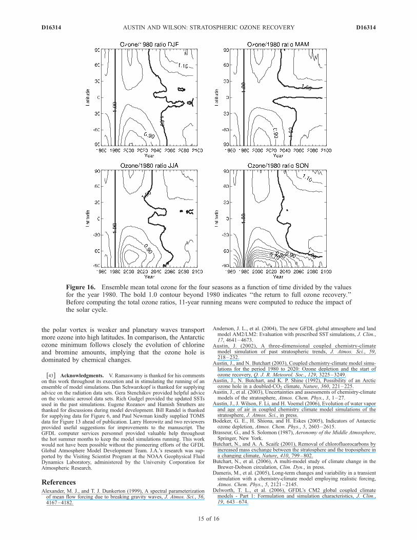
simulations predicted ozone amounts which are substantiallyhigher than simulated for 1980, particularly in the Arctic(Figure 15). This is due to the combined effects of decreasedhomogeneous ozone destruction from CO2 cooling andfurther increased strength of the Brewer-Dobson circulation.There is close consistency between the three ensemblemembers (not shown). Some of the details, such as theprecise location of the 1.0 ‘‘full recovery’’ contour in thetropics, suggest that the forcing data, especially the SSTs,are of prime importance.[35] The results for each of the four seasons are shown in

Figure 16. The solstice seasons are similar to each other andto the annual average, in indicating global ozone loss from1980 onward, especially in the polar regions. During theseseasons, full ozone recovery is also established on the sametime frame as in the annual average. However, for theequinox seasons, there are two main differences comparedwith the annual average relating to the failure of thesimulated ozone to return to 1980 values in all latitudesbefore the year 2095. During northern spring, tropical ozoneremained below 1980 levels in a narrow band. This is asmall effect and bearing in mind the absence of a Quasi-biennial Oscillation from the model dynamics may not be areliable result. A possibly larger consequence is the incom-plete recovery in spring ozone south of 75�S. The differ-ences in timing between the various diagnostics shown here(Figures 11–15) illustrate potential timing differences in thefuture real atmosphere. These differences indicate thatatmospheric ozone will likely have a different distributionof ozone in the future than in the past, a point made onprevious occasions [e.g., WMO, 2003, chapter 3]. The verylate recovery in Antarctic spring indicated in Figure 16 may

also simply be an idiosyncracy of our model, and hencewe await confirmation or otherwise from other modelsimulations.

7. Conclusions and Discussion

[36] Ensemble simulations of a high-resolution coupledchemistry-climate model have been presented for the period1960 to 2100. The period was split between the past (1960to 2005) in which each ensemble member was forced withobserved data (sea surface temperatures, SSTs; troposphericand volcanic aerosol, solar cycle and well-mixed green-house gases, GHGs), and the ‘‘future,’’ covering the period1990 to 2100. The future runs were forced with modelSSTs, background stratospheric aerosol amounts beyond1997, and the concentrations of the GHGs were taken fromthe A1B scenario. Results for the 15-year overlap period

Figure 13. Area of the Antarctic ozone hole in the model simulations in comparison with TOMS V8data as a function of year. Values have been averaged for the period 21–30 September. (left)Comparisons between TOMS 220 DU areas and AMTRAC 220 DU areas. (right) Comparisons betweenTOMS 220 DU areas and AMTRAC 175 DU areas.

Figure 14. Annual development of the Antarctic ozonehole area in the model by decade, based on the 220 DU totalozone contour. The broken lines indicate the axis ofmaximum values. The solid lines indicate the results fromthe ensemble mean of the future runs. The dotted linesindicate the mean of the results for the past runs.

D16314 AUSTIN AND WILSON: STRATOSPHERIC OZONE RECOVERY

13 of 16

D16314

were found to be consistent for most quantities despitedifferences in SSTs.[37] The past results were found to be sensitive to the

volcanic aerosol present, but this depended on the concen-tration of chlorine, in accordance with the work of Tie andBrasseur [1995]. Ozone increased after the eruption ofAgung, but reduced slightly after the eruption of El Chichonand more substantially following the eruption of MountPinatubo. Our results for the 1960s differ slightly from thoseof other recent model simulations [Dameris et al., 2005;C. Bruhl, personal communication, 2005] which gave onlya slight ozone increase during the Agung eruption. Thiscould be related to the impact of HOx catalyzed ozonedepletion which in our results is smaller due to a moremuted radiative effect of the Agung volcanic aerosol itself.[38] The solar cycle variation in ultraviolet also influ-

enced ozone amounts making it difficult to separate thevarious factors controlling the global ozone amounts. Toallow for these effects, ozone amounts were smoothed overthe 11-year solar cycle period. Minimum ozone occurredbetween 1998 and 2005 depending on ensemble memberwith no clear latitudinal dependence. Modeled past totalozone decreases since 1980 were almost twice the observedvalues of about 2–3% per decade outside the polar regionsand the overall model ozone was biased low. Nonetheless,the model reproduced many of the observed features of theatmosphere. In particular, the Antarctic ozone hole devel-oped rapidly in the model from about the late 1970s in goodagreement with observations and peak depletion occurredby about 2000–2005.[39] The simulated Antarctic ozone hole did not disappear

until about 2065 and a small residual ozone hole was

occasionally present up to a decade or more beyond that.During the recovery phase, interannual and ensemble var-iability of ozone was much larger than for the period ofozone hole formation, making the exact timing of recoverydifficult to determine. For reasons partially related tointerannual variability, the timing of the disappearance ofthe ozone hole depends critically on the precise definitionadopted. Correcting for the total ozone bias is complex.Assuming the usual ozone hole definition of 220 DU andallowing for a 45 DU bias in our simulations, tests wereapplied using a 175 DU ozone hole. This gives the mostfavored recovery date of 2065 specified above. However,taking a 30 DU bias, or 190 DU ozone hole criterion wouldimply that the model ozone hole would not have disap-peared until 2085. Even then, small ozone holes would bepredicted until the end of the century.[40] The definition of an ozone hole as that which occurs

when the ozone decreases below 220 DU is an arbitrary one,but instead full recovery can be defined as the return to1980 ozone values. If the model values are appropriatelytime-smoothed to eliminate solar effects and interannualvariability in the dynamics, the model was found not torecover fully in the Antarctic spring prior to the end of themodel simulation. This could be a highly model dependentresult, or a highly significant one for the biosphere if it isrealized in practice.[41] In the Arctic, model total ozone recovered to the

1980 column amount by about 2030 for the zonally aver-aged quantity and about 2040 for the seasonal minimumquantity. By this time interannual variability was also verylarge, but there was no sign of severe ozone depletion, ofAntarctic ozone hole standards, in any of the simulationscovering some 195 years for the period 1990–2030. There-fore it is predicted that the lowest ozone has alreadyoccurred or will be a small perturbation from the currentlowest levels. Again, AMTRAC is just one of many modelsthat is undergoing continual development to obtain im-proved results. The model intercomparison of Austin et al.[2003] showed large differences in the Arctic, and suchuncertainties will likely continue. All the same, it is impor-tant to note that there is a growing consensus [Austin et al.,2003] that further severe Arctic ozone depletion is unlikely.[42] On the multidecadal time frame, the impact of

climate change is an important issue. In the atmosphere,there will likely be an increase in the strength of the BrewerDobson circulation [Butchart and Scaife, 2001; Butchart etal., 2006]. This will increase the transport of CFCs into thestratosphere so that their atmospheric timescale will bereduced. The increased circulation is not fully taken intoconsideration by the tropospheric forcing values used in ourmodel simulations and would advance the timing for ozonerecovery by about a decade. Ozone recovery itself wouldrespond by partially reducing the change in the Brewer-Dobson circulation [Austin et al., 2006]. A more directimpact of climate change may be deduced by consideringthe different recovery timescales in the Arctic and Antarctic.The results obtained here suggest that Arctic ozone willrecover earlier than Antarctic ozone by some 25 to 35 years.The earlier Arctic recovery is a combined effect of bothincreased Brewer-Dobson circulation and reduced homoge-neous ozone depletion in a cooler stratosphere. Theseprocesses affect the Arctic more than the Antarctic because

Figure 15. Annual mean total ozone as a function of timedivided by the values for the year 1980 for the ensemblemean results. Dashed lines indicate the axis of minimumvalues, ‘‘the start of ozone recovery.’’ The 1.0 contourbeyond 1980 indicates ‘‘the return to full ozone recovery.’’Before computing the total ozone ratios, 11-year runningmeans were computed to reduce the impact of thesolar cycle. The shaded region indicates values greater than1.05.

D16314 AUSTIN AND WILSON: STRATOSPHERIC OZONE RECOVERY

14 of 16

D16314

the polar vortex is weaker and planetary waves transportmore ozone into high latitudes. In comparison, the Antarcticozone minimum follows closely the evolution of chlorineand bromine amounts, implying that the ozone hole isdominated by chemical changes.

[43] Acknowledgments. V. Ramaswamy is thanked for his commentson this work throughout its execution and in stimulating the running of anensemble of model simulations. Dan Schwarzkopf is thanked for supplyingadvice on the radiation data sets. Gera Stenchikov provided helpful adviceon the volcanic aerosol data sets. Rich Gudgel provided the updated SSTsused in the past simulations. Eugene Rozanov and Hamish Struthers arethanked for discussions during model development. Bill Randel is thankedfor supplying data for Figure 6, and Paul Newman kindly supplied TOMSdata for Figure 13 ahead of publication. Larry Horowitz and two reviewersprovided useful suggestions for improvements to the manuscript. TheGFDL computer services personnel provided valuable help throughoutthe hot summer months to keep the model simulations running. This workwould not have been possible without the pioneering efforts of the GFDLGlobal Atmosphere Model Development Team. J.A.’s research was sup-ported by the Visiting Scientist Program at the NOAA Geophysical FluidDynamics Laboratory, administered by the University Corporation forAtmospheric Research.

ReferencesAlexander, M. J., and T. J. Dunkerton (1999), A spectral parameterizationof mean flow forcing due to breaking gravity waves, J. Atmos. Sci., 56,4167–4182.

Anderson, J. L., et al. (2004), The new GFDL global atmosphere and landmodel AM2/LM2: Evaluation with prescribed SST simulations, J. Clim.,17, 4641–4673.

Austin, J. (2002), A three-dimensional coupled chemistry-climatemodel simulation of past stratospheric trends, J. Atmos. Sci., 59,218–232.

Austin, J., and N. Butchart (2003), Coupled chemistry-climate model simu-lations for the period 1980 to 2020: Ozone depletion and the start ofozone recovery, Q. J. R. Meteorol. Soc., 129, 3225–3249.

Austin, J., N. Butchart, and K. P. Shine (1992), Possibility of an Arcticozone hole in a doubled-CO2 climate, Nature, 360, 221–225.

Austin, J., et al. (2003), Uncertainties and assessments of chemistry-climatemodels of the stratosphere, Atmos. Chem. Phys., 3, 1–27.

Austin, J., J. Wilson, F. Li, and H. Voemel (2006), Evolution of water vaporand age of air in coupled chemistry climate model simulations of thestratosphere, J. Atmos. Sci., in press.

Bodeker, G. E., H. Shiona, and H. Eskes (2005), Indicators of Antarcticozone depletion, Atmos. Chem. Phys., 5, 2603–2615.

Brasseur, G., and S. Solomon (1987), Aeronomy of the Middle Atmosphere,Springer, New York.

Butchart, N., and A. A. Scaife (2001), Removal of chlorofluorocarbons byincreased mass exchange between the stratosphere and the troposphere ina changing climate, Nature, 410, 799–802.

Butchart, N., et al. (2006), A multi-model study of climate change in theBrewer-Dobson circulation, Clim. Dyn., in press.

Dameris, M., et al. (2005), Long-term changes and variability in a transientsimulation with a chemistry-climate model employing realistic forcing,Atmos. Chem. Phys., 5, 2121–2145.

Delworth, T. L., et al. (2006), GFDL’s CM2 global coupled climatemodels - Part 1: Formulation and simulation characteristics, J. Clim.,19, 643–674.

Figure 16. Ensemble mean total ozone for the four seasons as a function of time divided by the valuesfor the year 1980. The bold 1.0 contour beyond 1980 indicates ‘‘the return to full ozone recovery.’’Before computing the total ozone ratios, 11-year running means were computed to reduce the impact ofthe solar cycle.

D16314 AUSTIN AND WILSON: STRATOSPHERIC OZONE RECOVERY

15 of 16

D16314

Fioletov, V. E., G. E. Bodeker, A. J. Miller, R. D. McPeters, andR. Stolarski (2002), Global and zonal total ozone variations estimatedfrom ground-based and satellite measurements: 1964–2000, J. Geophys.Res., 107(D22), 4647, doi:10.1029/2001JD001350.

Groves, K. S., and A. F. Tuck (1980), Stratospheric O3-CO2 couplingin a photochemical-radiative column model. II With chlorine chemistry,Q. J. R. Meteorol. Soc., 106, 141–157.

Intergovernmental Panel on Climate Change (IPCC) (2001), ClimateChange 2001: The Scientific Basis. Third Assessment Report, edited byHoughton, J. T., et al., Cambridge Univ. Press, New York.

Knutson, T. R., T. L. Delworth, K. W. Dixon, I. M. Held, J. Lu,V. Ramaswamy, M. D. Schwarzkopf, G. Stenchikov, and R. J. Stouffer(2006), Assessment of twentieth-century regional surface temperaturetrends using the GFDL CM2 coupled models, J. Clim., 19, 1624–1651.

Labitzke, K., J. Austin, N. Butchart, J. Knight, J. Haigh, and V. Williams(2002), The global signal of the 11-year solar cycle in the stratosphere:Observations and model results, J. Atmos. Sol. Terr. Phys., 64, 203–210.

Miller, A. J., A. Cai, G. Tiao, and D. Wuebbles (2006), Examination ofozonesonde data for trends and trend changes including solar and arcticoscillation signals, J. Geophys. Res., 111, D13305, doi:10.1029/2005JD006684.

Newchurch, M. J., E. S. Yang, D. M. Cunnold, C. C. Reinsel, J. M.Zawodny, and J. M. Russell III (2003), Evidence for slowdown in strato-spheric ozone loss: First stage of ozone recovery, J. Geophys. Res.,108(D16), 4507, doi:10.1029/2003JD003471.

Newman, P. A., E. R. Nash, S. R. Kawa, S. A. Montzka, and S. M.Schauffler (2006), When will the Antarctic Ozone hole recover?, Geo-phys. Res. Lett., 33, L12814, doi:10.1029/2005GL025232.

Randel, W. J., F. Wu, S. J. Oltmans, K. Rosenlof, and G. E. Nedoluha(2004), Interannual changes of stratospheric water vapor and correlationswith tropical tropopause temperatures, J. Atmos. Sci., 61, 2133–2148.

Reinsel, G. C., A. J. Miller, E. C. Weatherhead, L. E. Flynn, R. M.Nagatani, G. C. Tiao, and D. J. Wuebbles (2005), Trend analysis oftotal ozone data for turnaround and dynamical contributions, J. Geo-phys. Res., 110, D16306, doi:10.1029/2004JD004662.

Sander, S. P., et al. (2003), Chemical kinetics and photochemical data foruse in atmospheric studies, Evaluation Number 14, JPL Publ., 02-25.

Shindell, D., D. Rind, N. Balachandran, J. Lean, and P. Lonergan (1999),Solar cycle variability, ozone and climate, Science, 284, 305–308.

Solomon, S., R. W. Portmann, T. Sasaki, D. J. Hofmann, and D. W. J.Thompson (2005), Four decades of ozonesonde measurementsover Antarctica, J. Geophys. Res., 110, D21311, doi:10.1029/2005JD005917.

Steinbrecht, W., H. Claude, and P. Winkler (2004), Enhanced upperstratospheric ozone: Sign of recovery or solar cycle effect?, J. Geophys.Res., 109, D02308, doi:10.1029/2003JD004284.

Steinbrecht, W., et al. (2006), Long-term evolution of upper stratosphericozone at selected stations of the Network for the Detection ofStratospheric Change (NDSC), J. Geophys. Res., 111, D10308,doi:10.1029/2005JD006454.

Tie, X., and G. Brasseur (1995), The response of stratospheric ozone tovolcanic eruptions: Sensitivity to atmospheric chlorine loading, Geophys.Res. Lett., 22, 3035–3038.

Weatherhead, E. C., et al. (2000), Detecting the recovery of total columnozone, J. Geophys. Res., 105, 22,201–22,210.

Wellemeyer, C. G., P. K. Bhartia, R. D. McPeters, S. L. Taylor, and C. Ahn(2004), A new release of data from the Total Ozone Mapping Spectro-meter (TOMS), SPARC Newsl. 22, pp. 37 – 38, SPARC Off., Serv.d’Aeron., Verrieres-le-Buisson, France.

World Meteorological Organization (WMO)/United Nations EnvironmentProgramme (UNEP) (2003), Scientific Assessment of Ozone Deple-tion: 2002, Rep. 47, Global Ozone Res. and Monit. Proj., Geneva,Switzerland.

Yang, E. S., M. Newchurch, D. Cunnold, R. J. Salawitch, M. P.McCormick, J. M. Russell III, J. Zadodny, and S. Oltmans (2006),Attribution of recovery in lower stratospheric ozone, J. Geophys.Res., doi:10.1029/2005JD006371, in press.

�����������������������J. Austin and R. J. Wilson, Geophysical Fluid Dynamics Laboratory,

Princeton, NJ 08542-0308, USA. (john.austin@noaa.gov)

D16314 AUSTIN AND WILSON: STRATOSPHERIC OZONE RECOVERY

16 of 16

D16314