Embed Size (px)
Citation preview

Characterizing Large Storage Systems: Error Behavior and PerformanceBenchmarks
by
Nisha Darshi Talagala
B.S. (Wayne State University) 1991M.S. (Wayne State University) 1992
A dissertation submitted in partial satisfaction of the
requirements for the degree of
Doctor of Philosophyin
Computer Science
in the
GRADUATE DIVISION
of the
UNIVERSITY OF CALIFORNIA, BERKELEY
Committee in Charge:
Professor David Patterson, ChairProfessor Randy Katz
Professor George Shanthikumar
Fall 1999
1
Abstract
Characterizing Large Storage Systems: Error Behavior and Performance Benchmarks
by
Nisha Darshi Talagala
Doctor of Philosophy in Computer Science
University of California, Berkeley
Professor David Patterson, Chair
This dissertation characterizes two causes of variability in a large storage system: soft
error behavior and disk drive heterogeneity. The first half of the dissertation focuses on
understanding the error behavior and component failure characteristics of a storage proto-
type. The prototype is a loosely coupled collection of Pentium machines; each machine
acts as a storage node, hosting disk drives via the SCSI interface. Examination of long
term system log data from this prototype reveals several interesting insights. In particular,
the study reveals that data disk drives are among the most reliable components in the stor-
age system and that soft errors tend to fall into a small number of well defined categories.
An in-depth study of hard failures reveals data to support the notion that failing devices
exhibit warning signs and investigates the effectiveness of failure prediction.
The second half of the dissertation, dealing with disk drive heterogeneity, focuses on a
new measurement technique to characterize disk drives. The technique, linearly increasing

2
strides, counteracts the rotational effect that makes disk drives difficult to measure. The
linearly increasing stride pattern interacts with the drive mechanism to create a latency vs.
stride size graph that exposes many low level disk details. This micro-benchmark extracts
a drive’s minimum time to access media, rotation time, sectors/track, head switch time,
cylinder switch time, number of platters, as well as several other pieces of information.
The dissertation describes the read and write versions of this micro-benchmark, named
Skippy, as well as analytical models explaining its behavior, results on modern SCSI and
IDE disk drives, techniques for automatically extracting parameter values from the graph-
ical output, and extensions.
-----------------------------------------------
Professor David Patterson
Dissertation Chair

iii
DEDICATION
To my parents, Rohana and Punya

iv
TABLE OF CONTENTS
CHAPTER 1. Chapter 1: Introduction ................................................................. 1
1.1. Thesis Goal................................................................................................. 21.2. Thesis Outline............................................................................................. 31.2.1. Characterizing Error Behavior ................................................................. 31.2.2. Characterizing Disk Drives...................................................................... 51.3. Thesis Contributions.................................................................................. 7
CHAPTER 2. The Storage System ........................................................................ 8
2.1. Introduction ................................................................................................ 82.2. Prototype Hardware.................................................................................... 92.3. Hardware Configuration........................................................................... 132.3.1. Node Design........................................................................................... 132.3.1.1. Performance Trade-offs of Varying the Disks/Host Ratio .................. 142.3.1.2. Problems with high Disk/Host Ratios ................................................. 162.3.2. Ethernet and Serial Interconnection....................................................... 172.3.3. Power Scheme........................................................................................ 192.3.4. Redundancy............................................................................................ 192.4. Application: A Web-Accessible Image Server ........................................ 192.4.1. Application Overview............................................................................ 192.4.2. File Format and User Interface .............................................................. 222.4.3. Disk Usage ............................................................................................. 232.5. Summary .................................................................................................. 24
CHAPTER 3. Characterizing Soft Failures and Error Behavior..................... 26
3.1. Introduction .............................................................................................. 263.2. Related Work............................................................................................ 273.3. Failure Statistics ....................................................................................... 283.4. Logs and Analysis Methodology.............................................................. 303.5. Results ...................................................................................................... 323.5.1. Error Types ............................................................................................ 333.5.2. Error Frequencies................................................................................... 373.5.3. Analysis of Reboots ............................................................................... 413.5.4. Correlations............................................................................................ 453.6. Discussion ................................................................................................ 473.7. Summary .................................................................................................. 49
CHAPTER 4. Characterizing Failures................................................................ 51
4.1. Introduction .............................................................................................. 514.2. Methodology ............................................................................................ 524.3. A Look At Failure Cases .......................................................................... 534.3.1. SCSI Cases............................................................................................. 53

v
4.3.2. Disk Drive Cases.................................................................................... 544.4. Effectiveness of Fault Prediction ............................................................. 554.4.1. The Dispersion Frame Technique.......................................................... 564.4.2. SCSI Cases............................................................................................. 584.4.3. Disk Drive Cases.................................................................................... 604.4.4. Discussion .............................................................................................. 624.5. Side Effects of Disk Drive Failures.......................................................... 644.6. Summary .................................................................................................. 65
CHAPTER 5. The Skippy Linear Stride Benchmark........................................ 66
5.1. Introduction .............................................................................................. 665.2. Background and Related Work ................................................................ 675.2.1. Disk Background ................................................................................... 685.2.2. Related Work ......................................................................................... 695.3. The Write Benchmark .............................................................................. 715.3.1. The Algorithm........................................................................................ 715.3.2. Graphical Result..................................................................................... 775.3.3. Extracting Parameters ............................................................................ 805.3.4. A Sample Result .................................................................................... 825.4. A Refined Analytical Model For Writes .................................................. 855.5. Write Measurements................................................................................. 875.5.1. SCSI Disk Drives ................................................................................... 885.5.2. Discussion .............................................................................................. 935.6. Read Benchmark ...................................................................................... 955.6.1. Expected Behavior ................................................................................. 965.6.2. Extracting parameters. ......................................................................... 1015.6.3. A Sample Result .................................................................................. 1025.7. Read Measurements ............................................................................... 1045.7.1. SCSI Disk Drives ................................................................................. 1045.7.2. IDE Disk Drives................................................................................... 1075.7.3. Discussion ............................................................................................ 1085.8. Summary ................................................................................................ 109
CHAPTER 6. Automatic Extraction ................................................................ 111
6.1. Introduction ............................................................................................ 1116.2. Approach ................................................................................................ 1126.3. Implementation Details .......................................................................... 1146.3.1. Phase I: Median Filter .......................................................................... 1146.3.2. Phase II: Identifying the line slope and transition points..................... 1156.3.3. Phase III: Identifying the head and cylinder switches ......................... 1176.3.4. Phase IV: Parameter calculation .......................................................... 1196.3.5. A Sample Result .................................................................................. 1196.4. Experiments............................................................................................ 1216.5. Optimizations ......................................................................................... 1226.5.1. Wider and Multiple Pass Filters........................................................... 123
vi
6.5.2. Using Alternative Cluster Algorithms ................................................. 1266.5.3. Using multiple extractions for accuracy checking............................... 1286.5.4. Combining the optimizations: A better algorithm ............................... 1296.6. Discussion .............................................................................................. 1296.7. Conclusion.............................................................................................. 131
CHAPTER 7. Extensions .................................................................................... 132
7.1. Introduction ............................................................................................ 1327.2. Extracting Global Disk Characteristics .................................................. 1337.2.1. Recording Zones .................................................................................. 1337.2.2. Seek Profile .......................................................................................... 1387.3. Extending the Skippy Technique ........................................................... 1417.3.1. Variable step size interval: Accuracy vs. Time Trade-off ................... 1427.3.2. Variable transfer size: Transfer Rate Measurement............................ 1447.3.3. The Backwards Read Benchmark........................................................ 1467.4. Other Issues ............................................................................................ 1477.4.1. Accuracy and Speed............................................................................. 1477.4.2. Cache Effects ....................................................................................... 1487.5. Summary ................................................................................................ 149
CHAPTER 8. Conclusion ................................................................................... 151
8.1. Summary ................................................................................................ 1518.1.1. Characterizing Soft Error Behavior ..................................................... 1518.1.2. Disk Drive Heterogeneity .................................................................... 1528.2. Future Directions.................................................................................... 1538.2.1. Understanding Error Behavior ............................................................. 1538.2.2. Understanding Disk Drive Heterogeneity........................................... 1548.3. Conclusion.............................................................................................. 155
vii
LIST OF TABLES
Table 2-1. Components Used in Storage Prototype.......................................... 10Table 2-2. Disk Enclosure Commands ............................................................. 12Table 3-1. Absolute Failures over 18 Months of Operation. ............................ 29Table 3-2. Sample Error Messages ................................................................... 34Table 3-3. Error Frequencies for 16 Machines over 6 Months ......................... 37Table 3-4. Total Number of Errors per Machine............................................... 40Table 3-5. Distribution of Restarts Across Machines ....................................... 43Table 3-6. Frequency of Each Type of Restart ................................................. 44Table 4-1. Summary: SCSI Failure Cases ........................................................ 54Table 4-2. Summary: Disk Drive Failure Cases ............................................... 55Table 4-3. DFT Prediction for SCSI Timeout Cases ........................................ 60Table 4-4. DFT Prediction for SCSI Parity Cases ............................................ 60Table 4-5. DFT Prediction for Disk Drive Cases.............................................. 61Table 4-6. Primary and Secondary Disk Error Messages ................................. 63Table 5-1. Parameters for Synthetic Disk Drive ............................................... 77Table 5-2. Description of the Disks in the Testbed........................................... 88Table 5-3. Extracted Parameters for SCSI Disk Drives .................................... 92Table 5-4. Parameters Extracted from Read Benchmark................................ 106Table 6-1. Percentage Errors of Manual and Automatic Extraction............... 120Table 7-1. SSE for Linear and Quadratic Fits to Zoned Results..................... 138
viii
LIST OF FIGURES
Figure 2-1. Storage Node Architecture............................................................... 14Figure 2-2. Performance Trade-Offs of Varying the Disks/Host Ratio .............. 15Figure 2-3. Interconnection and Power Topologies............................................ 18Figure 2-4. Image Server Operation ................................................................... 20Figure 2-5. GridPix Viewer ................................................................................ 23Figure 3-1. A Sample Line from Syslog Showing a SCSI TimeOut .................. 31Figure 3-2. Distribution of Errors by Machine over a Six Month Period........... 40Figure 3-3. Restarts and Their Causes................................................................ 43Figure 3-4. Network Errors over Time ............................................................... 46Figure 3-5. Other Errors over Time. ................................................................... 47Figure 3-6. Time Distribution of Restarts........................................................... 48Figure 4-1. Graphical Illustration of the Dispersion Frame Technique.............. 58Figure 4-2. Side Effects of Disk Failure ............................................................. 65Figure 5-1. Disk Drive Basics............................................................................. 68Figure 5-2. Pseudocode for the Write Version of Skippy. .................................. 71Figure 5-3. Sequence of Events for Two 1 Sector Writes .................................. 74Figure 5-4. Expected Skippy Result ................................................................... 78Figure 5-5. Illustrations of Behavior in Skippy Result....................................... 79Figure 5-6. Skippy Write Result for IBM UltraStar XP disk drive .................... 84Figure 5-7. Refined Model Result for Synthetic Disk ........................................ 87Figure 5-8. Skippy Write Result for 5400 RPM Seagate Hawk......................... 89Figure 5-9. Skippy Write Result for 7200 RPM Seagate Barracuda.................. 90Figure 5-10. Skippy Write Result for 7200 RPM Micropolis Drive .................... 91Figure 5-11. Skippy Write Result for 10000 RPM IBM 9ZX.............................. 91Figure 5-12. Skippy Write Result for 5400 RPM IBM IDE Drive....................... 93Figure 5-13. Skippy Write Result for 5400 RPM Quantum Fireball IDE Drive.. 94Figure 5-14. Read Model Result........................................................................... 99Figure 5-15. Illustrations of Request Behavior................................................... 100Figure 5-16. Other Possible Read Results .......................................................... 101Figure 5-17. Read Result for IBM UltraStar XP ................................................ 103Figure 5-18. Read Results for SCSI Disk Drives ............................................... 105Figure 5-19. Read Results for IDE Disk Drives ................................................. 108Figure 6-1. Classifications of Graph Regions................................................... 112Figure 6-2. Examples of Median Filters ........................................................... 115Figure 6-3. Median Filtered Graph................................................................... 116Figure 6-4. Removing the Linearly Increasing Offset ...................................... 118Figure 6-5. Extraction Accuracy....................................................................... 122Figure 6-6. Using Wider Filters and Multiple Passes ....................................... 125
ix
Figure 6-7. Using An Optimized Clustering Algorithm................................... 128Figure 6-8. Relative Errors of Optimized Algorithm ....................................... 130Figure 7-1. Pseudocode for Zoned Benchmark ................................................ 134Figure 7-2. Zoned Result on IBM UltraStar XP............................................... 134Figure 7-3. Zoned Results for SCSI Disk Drives ............................................. 136Figure 7-4. Linear and Quadratic Curve Fits for UltraStar XP Zoned Result .. 137Figure 7-5. Seek Measurement Algorithms...................................................... 140Figure 7-6. Seeker Result for Seagate Barracuda Drive ................................... 141Figure 7-7. Seeker Results for SCSI Disk Drives............................................. 142Figure 7-8. Effect of Increasing Step Interval Size .......................................... 144Figure 7-9. Effects of Increasing Transfer Size ................................................ 145Figure 7-10. Pseudocode for Backwards Read Benchmark ............................... 147Figure 7-11. Backwards Read Result for IBM UltraStar XP Drive ................... 147

x
ACKNOWLEDGEMENTS
Many people have helped and guided me through my time at Berkeley. The foremost of
these people is my advisor David Patterson. I am extremely lucky to have been able to
work with him. Dave helped me focus the direction of my research, while allowing me
the freedom to pursue my interests. His advising has been a great combination of technical
guidance, encouragement, and general good advice on all professional matters.
I would also like to thank my other readers, Randy Katz and George Shanthikumar, for
their advice during both my qualifying exam and dissertation. Randy Katz has always
been an inspiring influence, and has given me very good advice whenever I have inter-
acted with him. I was also fortunate to take a great course in Stochastic Processes from
George Shanthikumar.
I also owe thanks to Terry Lessard-Smith, Bob Miller, and Kathryn Crabtree, who have
saved me on many occasions in everything from registration matters to equipment.
Many thanks also to my fellow office mates in 477 Soda Hall, Remzi Arpaci-Dusseau and
Satoshi Asami. I have learned a great deal through working with each of them, and I’d
like to thank them for insightful comments, many fun discussions, and in all a friendly,
and memorable office environment. Thanks also to my other friends, in particular,
Sumudi, Rachel, and Manosha, who have been there for me throughout.
My husband, Amit, has been an essential background figure in this dissertation. In addi-
tion to giving me technical feedback and advice, he has been incredibly patient and given
me much emotional support and encouragement throughout my final years at Berkeley.
I owe a great debt to my parents. They instilled in me the importance of learning; they
have devoted their energy and made numerous personal sacrifices to enable me to study
in the United States. This dissertation would not have been possible without them.

xi
This research was funded by DARPA Grant N00600-93-K-2481, donations of equipment
from IBM and Intel, and the California State Micro Program.

1
1 Chapter 1: Introduction
The past decade has seen several fundamental changes in the field of I/O and storage sys-
tems. One of these changes was the invention of Redundant Arrays of Inexpensive Disks
(RAID) in 1988. The RAID work fueled a new class of disk-based storage systems con-
taining multiple disk drives with built in data redundancy. These innovations made it pos-
sible to construct large, multiple disk storage systems to serve I/O limited applications such
as video service. In 1999, eleven years later, RAID is a ten billion dollar industry, with
more than 50 companies making RAID-based subsystems. Storage systems research
during this time has also developed ways to improve the performance of RAID arrays, as
well as storage system designs for improving reliability.
However, modern applications, especially those derived from the web, require storage
infrastructures that are much larger than a simple disk-tape hierarchy containing a single
RAID system backed up by a single tape robot. Although stand-alone storage systems
range in capacity from hundreds of gigabytes to a few terabytes, large commercial instal-
lations contain terabytes to petabytes of data. This data is contained many storage arrays
on different hosts, many interconnected via switched networks. One of the largest unsolved

2
problems for such installations is not simply performance or reliability, but manageability.
Studies show that management of storage costs between twice to twelve times the cost of
the storage itself. Although management has traditionally been the task of system admin-
istrators, modern storage installations, with storage in thousands of disk drives, are far too
complex for human management.
Automated storage management is a large umbrella, covering everything from mainte-
nance, error reporting and diagnostics, to performance tuning. Solving these problems
requires that the storage system be adaptive, reacting correctly to the widely varying states
that the system will experience during its lifetime. A large part of an adaptive solution is
understanding and reacting to storage system variability. Even with a fixed architecture
and configuration, a storage system experiences considerable variability during its life-
time. This variability can result from a number of factors, including failures, component
and software upgrades, and so on.
1.1. Thesis Goal
The goal of this thesis is to assist the development of automated storage management by
characterizing storage system variability. In particular, the study focuses on two factors
that contribute to storage system variability, unexpected errors and heterogeneity in disk
drives.
(i) Error Behavior: Although much work has been done on designing storage systems to
tolerate failures of any component and combinations of components, not much work has

3
been done to characterize error behavior. Failures, however, are not binary events. Storage
systems exhibit a range of soft and hard errors, some leading to failure and some not. These
errors constantly change the state of the system, affecting both its performance and avail-
ability.
(ii) Disk Heterogeneity: Although a large system may be shipped with identical disk
drives, the disks in the infrastructure become more and more heterogeneous over time.
There are several reasons for this. First, as drives fail, they will be replaced by newer drives
that are considerably different. Second, the drive market evolves fast; a new disk appears
every nine to twelve months. Third, even if the drive mechanics remain unchanged, firm-
ware revisions appear every three to six months. Finally, a large installation is constantly
incrementing its storage by adding new subsystems. As a result, at any time, the installation
will contain many generations of disk drives, often from different manufacturers, and
hence will result in a heterogeneous system with disks of varying capacity and perfor-
mance.
1.2. Thesis Outline
This thesis characterizes the above two causes of storage system variability in the follow-
ing ways.
1.2.1. Characterizing Error Behavior
The first half of the thesis, chapters 2 through 4, deals with error behavior in a large storage
system. A terabyte capacity storage system prototype is described; the prototype contains
4
disks and supporting hardware such as SCSI controllers, network controllers and so forth.
The soft error and failure behavior of this prototype are then characterized, using system
logs and maintenance records gathered over six months of operation. The results reveal the
common types of errors that occur, the correlations between errors, and their effects on the
operating system and applications. The study also examines the events leading up to com-
ponent failure, as well as the distinction between transient errors and errors leading to fail-
ure.
Chapter 2 describes the storage system architecture used in this study. The prototype,
built by the Tertiary Disk group of the Network of Workstations (NOW) project, is a 3.2
TB system built from commodity hardware. The prototype contains 396 disks hosted by
20 PC and interconnected by a switched ethernet network. The application for this
storage system is a web server for high resolution art images. The collection, by far the
largest in the world, contains over 80,000 images and is available to users 24 hours a
day, 7 days a week at http://www.thinker.org/.
Chapter 3 describes the soft error behavior of the prototype. Six months of system logs
from the nodes of the prototype are analyzed to determine the types of errors that occur.
The analysis reveals some interesting insights. The data disks drives were among the most
reliable components in the system. Even though they were the most numerous component,
they experienced the lowest failure rate. Also, the study finds that all the errors observed
in six months can divided into eleven categories, comprising disk errors, network errors
and SCSI errors. The data supports the notion that disk and SCSI failures are predictable,
and suggests that partially failed SCSI devices can severely degrade performance.
5
Chapter 4 deals with failures in more detail. The chapter examines failure cases of disk
drives and SCSI hardware. Each case shows a noticeable increase in error messages before
replacement. The chapter also evaluates the effectiveness of a failure detection algorithm
developed by other researchers. The evaluation reveals that the algorithm tend to be over-
zealous, often reporting failures where none exist: transient errors can be labeled as failures
by such an algorithm. However, the type of message can be used to detect which events are
actually hardware failures and which are not.
1.2.2. Characterizing Disk Drives
The second half of the dissertation, chapters 5 through 7, presents a novel method for
extracting critical parameters from modern disk drives. The technique uses small disk
accesses, arranged in linearly increasing strides. The linearly increasing stride pattern
interacts with the disk mechanism in such a way that the resulting latency vs. stride size
graph explicitly illustrates many disk parameters. This micro-benchmark extracts a drive’s
minimum time to access media, rotational latency, sectors/track, head switch time, cylin-
der switch time, and the number of platters.
Chapter 5 describes the write and read versions of the basic linear stride micro-benchmark,
namedSkippy. The expected behavior of each version of the benchmark is described using
an analytical model. The analytical model verifies the technique and illustrates how drive
parameters can be extracted from the result graph. Measured results are presented on a
series of modern SCSI and IDE disk drives. The results show that the write version of the
benchmark is effective in extracting all the expected parameters, in all cases to within 3%
6
of values gathered from manufacturer specifications. The read version extracts the same
parameters with similar accuracy, and also provides some insight into how the drive han-
dles read ahead.
Chapter 6 describes an technique for automatically extracting the required parameters from
the result graph. This method is useful since it makes it possible for a higher level software
infrastructure, such as an adaptive storage system, to make use of theSkippy extraction
technique. The chapter describes the automated extraction tool and tests it on the results
from chapter 5. In most cases, the automatically extracted values are within 10% of their
manually extracted counterparts.
Chapter 7 presents extensions to the basicSkippy technique. Two additional algorithms,
Zoned andSeeker are presented.Zoned uses a bandwidth measurement to capture details
of the drive’s recording zones.Seeker shows how the linear stride technique can be used
to measure seek times. In addition, the chapter also presents howSkippy can be extended
by changing the transfer size and the stride size increment. With a larger transfer size,
Skippy can be used to measure the drive’s transfer rate. With larger stride size increments,
the same parameters can be extracted with fewer strides and in less time. Finally, the chap-
ter presents a read backwards stride micro-benchmark that retains the advantages of reads
without encountering read ahead effects.
7
1.3. Thesis Contributions
This dissertation makes the following contributions:
(i) Presents the first public, in-depth, analysis of soft error data from a terabyte-sized stor-
age system. The insights provided by this analysis are useful for any designer of a reliable
storage system.
(ii) Presents an in depth look at how devices fail. This type of data, again, is very hard to
come by, and is useful in the design of reliable storage systems. Evaluates the effectiveness
of failure prediction algorithms on large scale storage systems.
(iii) Presents a novel technique for extracting low level disk drive parameters using a
simple measurement that requires no a prior knowledge of the disk drive being measured.
This technique is also a good match to the rotational nature of the disk, a feature that makes
many other micro-benchmarks unsuitable for disk drives.
(iv) Presents extracted parameter values and performance data for a range of modern SCSI
and IDE disk drives. This data, and the measurement technique that generated it, and the
way the data is presented, are useful to the research community for parametrizing simula-
tors and understanding modern disk drives from a new perspective.

8
2 The Storage System
2.1. Introduction
This chapter describes the storage system prototype used in this thesis. The prototype, built
by the Tertiary Disk group of the Network of Workstations (NOW) project, is a 3.2 TB
system built from commodity hardware. The prototype contains 368 disks hosted by 20
PCs that are interconnected by a switched ethernet network. The main application for this
system is a web server for high resolution art images. The collection, by far the largest in
the world, contains over 80,000 images and is available to users 24 hours a day, 7 days a
week at http://www.thinker.org/.
Commodity storage systems, like the TD prototype, have several advantages over custom
designed disk arrays. For one thing, the cost/megabyte of disk arrays increases with capac-
ity and, in most cases, is higher than the cost/megabyte of the underlying disks. Disk array
costs are high because they contain custom designed hardware. In 1999, disks cost as little
as 5 cents per megabyte, close to the cost of tape libraries [Grochowski96, IDEMA97].
Although disk prices are falling by 50% every year, the cost/megabyte of disk arrays is not
falling as quickly. Secondly, performance of disk arrays is limited by the bandwidth of the
link to the host machine. Finally, incremental expansion in a disk array is possible only

9
until all available disk slots are filled. For these reasons, a commodity storage system made
up of relatively independent nodes is a plausible alternative to custom designed disk array.
The node-based design makes adding disks and nodes easier. The cost/megabyte of the
system stays relatively constant even as the capacity grows. The nodes also provide multi-
ple connections to the outside world, improving performance and availability. The proto-
type proves by example that storage systems using commodity hardware can be built for a
small extra cost over the underlying disks and provides a basis for the studies on error
behavior that make up the first part of the thesis.
This chapter covers the prototype’s architecture and application. This information is useful
as perspective for the chapters that follow. Section 2.2 describes the prototype hardware in
detail. The next section covers the hardware configuration, designs of nodes, interconnec-
tions and power scheme. Section 2.4 describes the application, including data layout and
user activity. Finally section 2.5 concludes with a summary.
2.2. Prototype Hardware
Table 2-1 describes the components used in the prototype. All components are the state of
the art as of 1996, when work on the prototype first began. The twenty PCs that host the
storage are interconnected using a switched Ethernet network. In addition, there is a sepa-
rate serial network that is use for management, connecting PCs, disk enclosures and UPS
units. Each PC has four PCI expansion slots on the motherboard (most PCs available at the
time of this writing contain three or four PC expansion slots). The PCI slots contain two
10
twin-channel Fast-Wide SCSI adapters and an Ethernet card. Power and cooling for the
disks is provided by disk enclosures. All the enclosures, host machines, and network com-
ponents are housed in a series of racks. Power to the system is supplied through Uninter-
uptible Power Supply (UPS) units.
The Pentium Pro machines were chosen over other alternatives (such as SPARCStation-5s
and UltraSPARCs) because PCs are naturally well equipped for hosting disks. The main
system bus, PCI, has a peak bandwidth of 132 MB/s, compared to 90 MB/s for the Sbus,
which was the main alternative available at the time. PCs also have more expansion slots
than either the SPARCStation 5 or the UltraSPARC: three or four compared to two in each
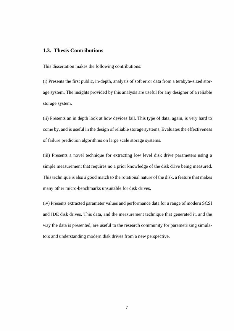
Component typeNumber Used inPrototype Description
Host machines 20 Pentium Pro 200 MHz, 96 MB main memory, 1GB SCSI hard drive, PCI bus, 4 PCI expansionslots, 3 ISA slots.
SCSI Disks 368 IBM Ultrastar XP, 8 GB, 7200 RPM, SCSI
IDE Disks 20 Seagate ST32140A 2GB 5400RPM IDE
SCSI Controllers 40 Adaptec 3940 Twin Channel UW SCSI
Disk Enclosures 48 Sigma Trimm Model SA-H381, Dual powersupplies. Each enclosure holds 7-8 disks.
Uninteruptible Power Supplies 6 Powerware Prestige 6000 Units
Ethernet Controller 20 3Com Fast Etherlink PCI 10/100 BASE-TAdapters
Ethernet Hub 2
Serial Port Hub 2 Bay Networks 5000 Hub
Other equipment - Miscellaneous Cables (SCSI, Ethernet, Serial),SCSI Terminators
Table 2-1. Components Used in Storage Prototype
The main components are the disks, SCSI controllers, host machines, disk enclosures, net-work hardware and uninteruptible power supplies. This table gives the model numbers andother information for each main components.
11
of the alternative machines. In addition, PCs were the most cost effective of the three
choices. The PC model used in the prototype was not preferred over the other PC models
for any reason. They were used because they were part of a donation by Intel.
Fast-Wide SCSI was chosen because it was the highest performance disk interconnect
available at the time. Serial interconnects with higher bandwidth, 40-100MB/s compared
to 20 MB/s for SCSI, had been introduced. However, disks and controllers using these
interfaces were not yet widely available. Twin-channel SCSI adapters were used because
each PC could host more SCSI strings with twin channel adapters than with single channel
adapters; each PCI expansion slot can host two SCSI strings instead of one. Performance
measurements comparing single and twin channel SCSI controllers revealed no noticeable
performance losses when using twin channel controllers.
Power and cooling for the disks is provided by the disk enclosures. Each enclosure hosts
up to seven disks. All enclosures are connected through a serial port hub. This way, any
enclosure can be accessed remotely, and the status of all enclosures can be monitored from
a remote location. The serial port interface supports a small set of commands; Table 2-2
lists the commands supported by our enclosures. The commands return the status of the
enclosure (power supplies, disks an so on) and control the LEDs above each disk slot.
When a disk needs to be replaced, the enclosure can be programmed to turn the LED above
the failed disk to red, making it easier for the disk to be identified. The enclosures are the
only components that are not strictly commodity. The serial port interface and other fea-
tures, like dual power supplies, were included because they make maintenance and moni-
toring easier. The additional features make the enclosures a special order item, and not

12
strictly commodity. However, standard disk enclosure models are also available by com-
panies like Sigma/Trimm.
The Uninteruptible Power Supplies provide 10 minutes of backup power to the nodes. This
feature is useful both for surviving short power glitches and for allowing time for safe shut-
down on power failure. The UPS units also provide a serial interface that can be polled to
detect power failure events.
Command Name Command DescriptionCommandCharacters Result/Return
Hello Start of communications Ctrl-A Acknowledgment by chassis
Inquiry Request for identification Ctrl-E Acknowledgment followed by the enclo-sure model number and firmware revision.
Status Request for status S Acknowledgment followed by 8 data bytesof status information
Change Drive LEDs Change the status of anLED to indicate faileddrives
D, 1 data byte Acknowledgment from chassis, the LEDof the specified drive is changed in color(red to green or vice versa)
I/O control Control the mute-buttoncapture latch (can be usedto detect when an operatoris standing by)
I, 1 data byte Acknowledgment from chassis
SCSI Bus Reset Assert/Release the SCSIbus reset line
R, 1 data byte Acknowledgment from chassis; therequested reset/release action takes place
N/A Misunderstood charactersequences
All other charactercombinations
Negative acknowledgment from chassis
Table 2-2. Disk Enclosure Commands
These commands are used to communicate with the disk enclosure over a serial port. Moredetails are available in [Sigma97]; the encoding of the status bytes and the data bytes isdescribed there. The mute button is a special button on the enclosure that stops the alarmfrom sounding. The mute button capture latch catches all mute button presses and is usedto detect an operator standing by an enclosure.

13
2.3. Hardware Configuration
This section describes the hardware configuration of the storage system, beginning with a
description of the storage node architecture and ending with a discussion of the intercon-
nection and power schemes.
2.3.1. Node Design
The prototype has two types of nodes, which from now on will be called light nodes and
heavy nodes. The prototype has sixteen light nodes and four heavy nodes. Each light node
contains 16 disks on 2 SCSI strings while each heavy node has 28 disks on 2 SCSI strings.
There are cost and performance trade-offs in changing the disks/host ratio, as well as addi-
tional problems with large numbers of disks. The light nodes have a higher cost and better
performance than the heavy nodes. As the disks/host ratio is increased, the cost/megabyte
of the node becomes closer to the cost/megabyte of the disks, making the heavy nodes
more cost-effective.
Figure 2-1 shows the internal hardware architecture of a storage node. For clarity, the
figure shows only one SCSI string. In the heavy nodes, the 14 disks on each string are
housed in two disk enclosures of 7 disks each; in the light nodes, each SCSI string has 8
disks housed in a single enclosure. Disks plug directly into the enclosure’s backplane,
which contains the SCSI bus, a design that reduces the SCSI cable length within the disk
enclosure. The SCSI bus is made up of the SCSI cable, starting at the SCSI controller and
ending as the enclosure backplane. Each enclosure is powered by two power supplies and
cooled with a single fan. Each machine also contains a single Ethernet card and a cable
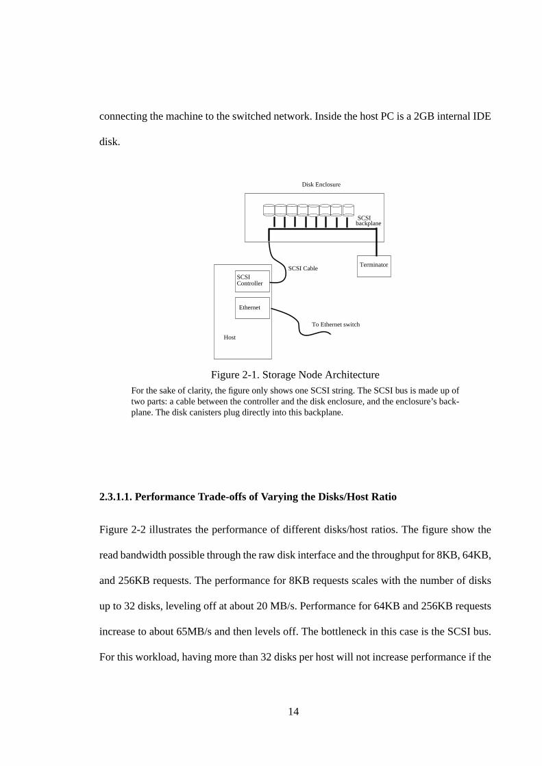
14
connecting the machine to the switched network. Inside the host PC is a 2GB internal IDE
disk.
2.3.1.1. Performance Trade-offs of Varying the Disks/Host Ratio
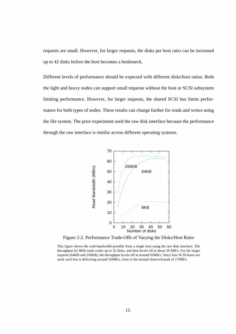
Figure 2-2 illustrates the performance of different disks/host ratios. The figure show the
read bandwidth possible through the raw disk interface and the throughput for 8KB, 64KB,
and 256KB requests. The performance for 8KB requests scales with the number of disks
up to 32 disks, leveling off at about 20 MB/s. Performance for 64KB and 256KB requests
increase to about 65MB/s and then levels off. The bottleneck in this case is the SCSI bus.
For this workload, having more than 32 disks per host will not increase performance if the
Figure 2-1. Storage Node ArchitectureFor the sake of clarity, the figure only shows one SCSI string. The SCSI bus is made up oftwo parts: a cable between the controller and the disk enclosure, and the enclosure’s back-plane. The disk canisters plug directly into this backplane.
Disk Enclosure
ControllerSCSI
Ethernet
Host
Terminator
SCSIbackplane
SCSI Cable
To Ethernet switch
15
requests are small. However, for larger requests, the disks per host ratio can be increased
up to 42 disks before the host becomes a bottleneck.
Different levels of performance should be expected with different disks/host ratios. Both
the light and heavy nodes can support small requests without the host or SCSI subsystem
limiting performance. However, for larger requests, the shared SCSI bus limits perfor-
mance for both types of nodes. These results can change further for reads and writes using
the file system. The prior experiment used the raw disk interface because the performance
through the raw interface is similar across different operating systems.
Figure 2-2. Performance Trade-Offs of Varying the Disks/Host Ratio
This figure shows the read bandwidth possible from a single host using the raw disk interface. Thethroughput for 8KB reads scales up to 32 disks, and then levels off at about 20 MB/s. For the largerrequests (64KB and 256KB), the throughput levels off at around 65MB/s. Since four SCSI buses areused, each bus is delivering around 16MB/s, close to the normal observed peak of 17MB/s.
0
10
20
30
40
50
60
70
0 10 20 30 40 50 60
Rea
d B
andw
idth
(M
B/s
)
Number of disks
8KB
64KB256KB
16
2.3.1.2. Problems with high Disk/Host Ratios
Since PCs are not normally required to support such a large number of disks, unexpected
problems may crop up when the disk/host ratio becomes larger. A few problems that we
encountered are listed below:
(i) Operating system and firmware bugs: Since most PC operating systems were not
designed to host large numbers of disks, increasing the disks/host ratio can expose undis-
covered problems in operating system and disk controller software. While developing our
prototype, we ran across several such problems. Windows NT, for instance, supports only
31 disks through its Disk Administrator GUI. Versions of Solaris x86 that we experi-
mented with had problems with more than 7 disks on a SCSI string. We also discovered an
Adaptec firmware bug that did not allow 15 disks on both strings of a twin channel SCSI
adapter. More details on these issues are available in [Talagala96].
(ii) SCSI Limits: Since the maximum length of a Fast-Wide SCSI string is about 9 feet, if
a SCSI string is longer, time-outs and other problems can occur. If the string is not properly
terminated, these problems can happen with shorter buses as well. We were able to keep
the string length short inside an enclosure by having the SCSI bus on the enclosure back-
plane. If the SCSI bus is not on the enclosure backplane, cabling between disks inside the
enclosure can add to the total string length. Differential SCSI allows longer cable lengths
(up to almost 80 feet), making string length less of a problem. Serial interconnects will also
allow very long strings [Schwarderer96].

17
(iii) Host Machine Limits: Most PCs have at most four PCI slots, placing a limit on the
number of disks that can be connected to it. In this case PCI-PCI bridges can be used to
extend the host PCI bus.
Because of such problems, we were not able to reliably connect more than 56 disks to a
single node. As the prior section indicated, increasing the disks/host ratio beyond this limit
also makes the host and SCSI subsystem a performance bottleneck.
2.3.2. Ethernet and Serial Interconnection
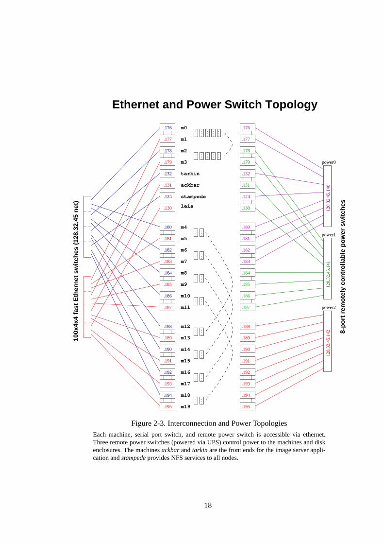
All nodes are connected via 100Mbit Switched Ethernet. Figure 2-3 shows the Ethernet
and Power Switch topology for the prototype. The subnet contains two Ethernet switch
hubs. The host machines are named m0-m19; each machine has its own ethernet address.
The heavy nodes are m0-m3 and the light nodes are m4-m19. The subnet contains four
additional machines. Two of these machines provide NFS, home directories, and naming
services for the storage cluster. The last two machines, namely ackbar and tarkin, are front
ends for the image server application. Their use is discussed further in section 2.4. Finally,
each remotely controlled power switch also occupies an ethernet address.
In addition to Ethernet, all machines are also connected via serial lines that provide an
alternative way to access the machines for easier management. For simplicity, all serial
connections are routed through a single serial port concentrator. This concentrator has four
24 port serial terminal servers, each with its own ethernet connection. This single hub is a
possible point of failure; however this is not much of a problem since the serial lines are
intended only for monitoring and management, not for data transfer. The disk enclosures
and UPS (Uninteruptible Power Supply) Units are also interconnected with serial lines.
18
Figure 2-3. Interconnection and Power TopologiesEach machine, serial port switch, and remote power switch is accessible via ethernet.Three remote power switches (powered via UPS) control power to the machines and diskenclosures. The machines ackbar and tarkin are the front ends for the image server appli-cation and stampede provides NFS services to all nodes.
Ethernet and Power Switch Topology
m7
m8
m9
m10
m11
m12
m13
m14
m15
m16
m17
m18
m19
m1
m2
m3
tarkin
ackbar
stampede
leia
m4
m5
m6
.179
.131
.130
.176
.132
.124
.180
.182
.195
.193
.191
.189
.194
.192
.190
.188
.177
.181
.183
.178
.184
.185
.186
.187
128.
32.4
5.14
112
8.32
.45.
140
128.
32.4
5.14
2
power1
power2
power0
8-p
ort
rem
ote
ly c
on
tro
llab
le p
ow
er s
wit
ches
m0.176
.177
.178
.179
.132
.131
.124
.130
.180
.181
.182
.183
.184
.185
.187
.188
.189
.190
.191
.192
.193
.194
.195
100x
4x4
fast
Eth
ern
et s
wit
ches
(12
8.32
.45
net
)
.186

19
2.3.3. Power Scheme
Figure 2-3 also shows how power is routed to the cluster. Each disk enclosure contains two
power supplies. In addition, power protection is provided for the entire cluster via the six
UPS units. The power scheme is completed by the remotely controllable power switches
that enable automatic hard resets of each machine.
2.3.4. Redundancy
The data served by the image server is mirrored across the nodes. The dotted lines in figure
2-3 identify pairs of mirror nodes. As the figure shows, the configuration strives to provide
independent network paths and power paths to node in a mirrored pair.
2.4. Application: A Web-Accessible Image Server
The storage cluster hosts a web-accessible image server. This service, called The Zoom
Project, has been available to users since March 1st 1998. This site, a collaborative effort
between UC Berkeley and the Fine Arts Museums of San Francisco, provides a database
of over 80,000 high resolution images of art work. Each image is available at resolutions
of up to 3072x2048 pixels. It is by far the largest on-line art collection in the world.
2.4.1. Application Overview
Figure 2-4 shows how the site works. The front end, at http://www.thinker.org/, is hosted
by the Fine Arts Museum. Each image is searchable by title, artist, time period, and other
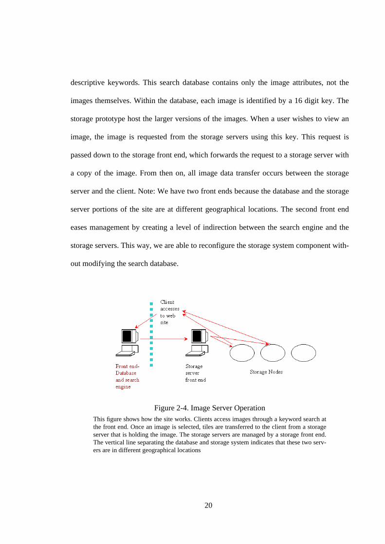
20
descriptive keywords. This search database contains only the image attributes, not the
images themselves. Within the database, each image is identified by a 16 digit key. The
storage prototype host the larger versions of the images. When a user wishes to view an
image, the image is requested from the storage servers using this key. This request is
passed down to the storage front end, which forwards the request to a storage server with
a copy of the image. From then on, all image data transfer occurs between the storage
server and the client. Note: We have two front ends because the database and the storage
server portions of the site are at different geographical locations. The second front end
eases management by creating a level of indirection between the search engine and the
storage servers. This way, we are able to reconfigure the storage system component with-
out modifying the search database.
Figure 2-4. Image Server OperationThis figure shows how the site works. Clients access images through a keyword search atthe front end. Once an image is selected, tiles are transferred to the client from a storageserver that is holding the image. The storage servers are managed by a storage front end.The vertical line separating the database and storage system indicates that these two serv-ers are in different geographical locations

21
The storage front end is implemented by the machines tarkin.cs and ackbar.cs that back
each other up using IP aliasing. All requests are directed to the canonical address
gpx.cs.berkeley.edu. When tarkin.cs is up and running, it handles all requests to this
address. tarkin.cs is constantly monitored by ackbar.cs. If tarkin.cs goes down, then sec-
ondary takes over by assuming the gpx.cs.berkeley.edu address. Once tarkin.cs comes back
up, ackbar.cs gives up the gpx address. The front ends maintain a directory of image IDs
and storage servers. In addition, the front ends periodically monitor the storage servers and
maintains lists of non-responding servers. When a storage server goes down, all image
requests are forward to the server with the mirror copy of the image.The requests are for-
warded from the front ends to the storage servers using HTTP-redirect. Each host in the
prototype serves its local images using the Apache Web Server.
Unlike prior file-service based storage systems architectures, this failover design does not
attempt to mask failures for client connections that are already in progress. This decision
reflects the design principle that for this type of web-based application, Fix-By-Reload is
the necessary level of availability. Studies have shown that the when internet users expe-
rience slowdowns, the problem is far more likely to be the connection to the web server
than the server itself [Manley97]. Since the user’s only means of access is through a slow
and unreliable link, they are capable of retrying requests that time-out or fail. Therefore,
for users coming over the web, the only availability requirement that the system must
meet is to recover within enough time to satisfy the request retry. In particular, it is not
necessary to mask all failures at the site. In many cases, no matter how reliable the web
server, the internet will generate failures that are visible to the user. Prior work on smart
clients has shown that it is possible for the client browser to do fault tolerance by switch-

22
ing between several sites that are offering the same service [Yoshikawa97]. This idea can
also be used to build an automatic retry mechanism into the browser so that the user does
not even have to click reload when a failure occurs.
Once the user specifies a screen size, a 12.5% resolution version of the image appears
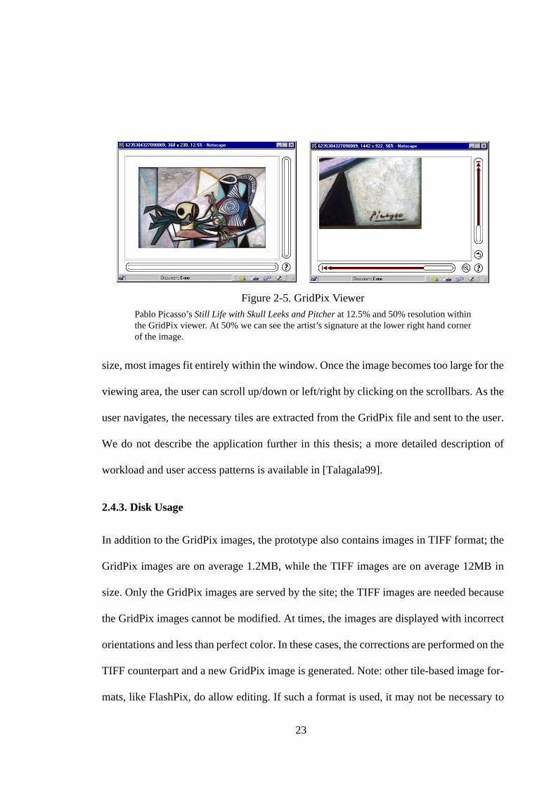
inside a zoom window. Figure 2-5 shows Picasso’s Still Life with Skull, Leeks and Pitcher
in zoom windows at 12.5% and 50% resolutions. We can see the Picasso signature by
zooming into a corner of the painting. Once the image becomes too large to fit in the win-
dow, scrollbars appear. Users can zoom in up to 1600% resolution, 16 times the art work’s
full size.
2.4.2. File Format and User Interface
The images are stored in a tiled format called GridPix [Asami98], similar in concept to the
FlashPix standard [Kodak97]. Both formats have the notions of tile-based images and mul-
tiple image resolutions within a single file. The difference is that GridPix is a simpler
format designed only for storing tiled images, while FlashPix is a more generalized format
designed with many different uses in mind. A GridPix file contains a header structure, an
index of offsets, and a sequence of JPEG encoded image tiles in resolutions from 12.5% to
100%. Tiles for resolutions higher than 100% are generated on the fly from the 100% res-
olution tiles. The GridPix file format and associated software is discussed in more detail in
[Asami98].
The viewer is implemented by two CGI programs; one creates the graphical viewer and the
second retrieves each tile. The viewer places the tiles adjacent to each other in the HTML
page to create the full image. All images are initially displayed at 12.5% resolution. At this
23
size, most images fit entirely within the window. Once the image becomes too large for the
viewing area, the user can scroll up/down or left/right by clicking on the scrollbars. As the
user navigates, the necessary tiles are extracted from the GridPix file and sent to the user.
We do not describe the application further in this thesis; a more detailed description of
workload and user access patterns is available in [Talagala99].
2.4.3. Disk Usage
In addition to the GridPix images, the prototype also contains images in TIFF format; the
GridPix images are on average 1.2MB, while the TIFF images are on average 12MB in
size. Only the GridPix images are served by the site; the TIFF images are needed because
the GridPix images cannot be modified. At times, the images are displayed with incorrect
orientations and less than perfect color. In these cases, the corrections are performed on the
TIFF counterpart and a new GridPix image is generated. Note: other tile-based image for-
mats, like FlashPix, do allow editing. If such a format is used, it may not be necessary to
Figure 2-5. GridPix ViewerPablo Picasso’s Still Life with Skull Leeks and Pitcher at 12.5% and 50% resolution withinthe GridPix viewer. At 50% we can see the artist’s signature at the lower right hand cornerof the image.
24
keep other formats around. However, in our experience, a large and constantly evolving
image database will contain images in several formats.
Each disk is divided into three key partitions. The first is a 32KB partition that contains
start-up scripts for each disk. These scripts are to identify the disk at boot time; they are
described in more detail in [Asami99]. The second partition is 1GB and is used for various
experiments. The third partition occupies the bulk of the disk, 7GB, and is used for image
storage. On each storage server, the third partition of all the disks are organized as a striped
disk array using the CCD (Concatenated Disk Driver) pseudo device driver. The GridPix
image files are stored on a BSD Fast-File System (BSD FFS) on this striped disk array
[BSD96].
The 2GB internal drive contains the operating system and swap area for each node. In addi-
tion, each node mounts shared NFS filesystems from the infrastructure servers. These file
systems contain software tools and home directories for the system’s users.
2.5. Summary
This chapter described the storage system prototype and its application. The prototype con-
sists of a group of relatively independent nodes interconnected by a switched network.
Directed by a front end, the nodes collectively form a web-accessible image database for
the high resolution art images of the Fine Arts Museums of San Francisco. The prototype
is used to study the soft error behavior in a large storage system; these studies are described

25
in the next two chapters. In addition, the prototype’s disks are used in the studies on disk
performance variability in chapters 5 and 6.
26
3 Characterizing Soft Failures and
Error Behavior
3.1. Introduction
This chapter presents data on the soft failure characteristics of the prototype. We analyze
system error logs from the storage system described in Chapter 2. We describe the soft
error behavior of disks and SCSI components, the effects of component failures on the
operating system of the host machine, and the effects of network failures. We also corre-
lation between soft errors on different storage nodes.
The analysis leads to some interesting insights. We found that the SCSI disk drives were
among the most reliable components in the system. Even though they were the most
numerous component, they experienced the lowest failure rate. Also, we found that all the
errors observed in six months can divided into eleven categories, comprising disk errors,
network errors and SCSI errors. We also gained insight into the types of error messages
reported by devices in various conditions, and the effects of these events on the operating
system. Our data supports the notion that disk and SCSI failures are predictable, and sug-
27
gests that partially failed SCSI devices can severely degrade performance. Finally, we
observed the disastrous effects of single points of failure in our system.
The rest of the chapter is organized as follows. Section 3.2 outlines related work. Section
3.3 describes the statistics on absolute failures for the prototype over 18 months of opera-
tion. Absolute (or hard) failures are cases where the component was replaced. These sta-
tistics provide a useful perspective for the study on soft errors that makes up the rest of the
chapter. Section 3.4 describes the logs used to gather soft error information. Section 3.5
describes the results obtained from studying these logs. Section 3.6 discusses the results
and their implications. Finally Section 3. 7 concludes with a summary.
3.2. Related Work
There has been little data available on the reliability of storage system components. An ear-
lier study [Tsao83] suggested that system error logs can be used to study and predict
system failures. This work focused on filtering noise and gathering useful information
from a system log. The authors introduced the “tuple concept”; they defined a tuple as a
group of error records or entries that represent a specific failure symptom. A tuple contains
the earliest recorded time of the error, the spanning time, an entry count, and other related
information. The work described a Tuple Forming Algorithm, to group individual entries
into Tuples, and a Tuple Matching Algorithm to group tuples representing the same failure
symptom. The study did not attempt to characterize the failure behavior of devices, and
was not specifically targeted at storage systems. Follow up work characterized the distri-
28
butions of various types of errors and developed techniques to predict disk failures [Lin90].
In this study, the system was instrumented to collect very detailed information on error
behavior [Lin90]. The DFT algorithm, a failure prediction algorithm developed in this
work, is used in the next chapter as part of a study of device failures.
A second study associated with the RAID effort [Gibson88] [Shulze89] presented factory
data on disk drive failure rates. This study focused on determining the distribution of disk
drive lifetimes. The authors found that disk drive lifetimes can be adequately characterized
by an exponential distribution. A third study, an analysis of availability of Tandem systems
was presented in [Gray90]. This work found that software errors are an increasing part of
customer reported failures in the highly available systems sold by Tandem.
Most recently, disk companies have collaborated on the S.M.A.R.T (Self, Monitoring,
Analysis and Reporting Technology) standard [SMART99]. SMART enabled drives mon-
itoring a set of drive attributes that are likely to degrade over time. The drive notifies the
host machine if failure is imminent.
3.3. Failure Statistics
We begin with statistics on absolute hardware failures for eighteen months of the proto-
type’s operation (from March 1997 to August 1998). Table 3-1 shows the number of com-
ponents that failed within this one and a half year time frame. For each type of component,
the table shows the number in the entire system, the number that failed, and the percentage
failure rate. Since our prototype has different numbers of each component, we cannot

29
directly compare the failure rates. However, we can make some qualitative observations
about the reliability of each component.
Our first observation is that, of all the components that failed, the data disks are the most
reliable. Even though there are more data disks in the system than any other component,
their percentage failure rate is the lowest of all components. The enclosures that house
these disks, however, are among the least reliable in the system. The disk enclosures have
two entries in the table because they had two types of failure, power supply problems and
SCSI bus backplane integrity failures. The enclosure backplane has a high failure rate
while the enclosure power supplies are relatively more reliable. Also, since each enclosure
Component Total in System
Total Failed(AbsoluteFailures) % Failed
SCSI Controller 44 1 2.3%
SCSI Cable 39 1 2.6%
SCSI Disk 368 7 1.9%
IDE Disk 24 6 25.0%
Disk Enclosure 48 13 28.3%
Enclosure Power 92 3 3.26%
Ethernet Controller 20 1 5.0%
Ethernet Switch 2 1 50.0%
Ethernet Cable 42 1 2.3%
Total Failures 34
Table 3-1. Absolute Failures over 18 Months of Operation.
For each type of component, the table shows the total number used in the system, thenumber that failed, and the percentage failure rate. Note that this is the failure rate over 18months (it can be used to estimate the annual failure rate). Disk enclosures have twoentries in the table because they experienced two types of problems, backplane integrityfailure and power supply failure. Since each enclosure had two power supplies, a powersupply failure did not affect availability. As the table shows, the SCSI data disks areamong the most reliable components, while the IDE drives and SCSI disk enclosures areamong the least reliable. Note that this table does not show the same number of compo-nents as Table 2-1 since it lists the total number of components used over the 18 monthtime frame.
30
has two power supplies, a power supply failure does not incapacitate the enclosure. The
IDE internal disks are also one of the least reliable components in the system, with a 25%
failure rate. The unreliability of the IDE disks could be related to their operating environ-
ment. While the SCSI drives are in enclosures specially designed for good cooling and
reduced vibration, the IDE drives are in regular PC chassis. Overall, the system experi-
enced 34 absolute failures in eighteen months, or nearly two absolute failures every month.
We note that Table 3-1 only lists components that failed over eighteen months (Table 2-1
lists all hardware components in the prototype). Some components had no failures at all in
this time frame. These components include the PC internals other than the disk (the moth-
erboard, power supply, memory modules, etc.), serial hardware, UPS units an so on.
3.4. Logs and Analysis Methodology
The operating system reports error messages, boot messages, and other status messages to
the internal system log. The kernel, system daemons, and user processes can contribute to
this log using the syslog and logger utilities [FreeBSD97]. These logs are located at /var/
log/messages in our configuration of FreeBSD 2.2. We studied these logs to gather
information about soft failure behavior.
We began by filtering out messages that reported status and login information. To this end,
we removed all messages from sshd (secure shell logins), sudo messages, other login mes-
sages, and all boot messages. This preprocessing reduced the size of the logs between 30%

31
and 50%. The messages that remained were primarily from the OS kernel and network dae-
mons.
Figure 3-1 shows a sample error message from a system log that is reporting a timeout on
the SCSI bus. This log line has seven pieces of information. The first three fields contain
the date and time. The fourth field is the machine name, in this case m2. The fifth field lists
the source of the message; in this case the operating system kernel is reporting the error.
The sixth field specifies the device on which the timeout occurred. The first two subfields
of the sixth field specify the disk number and SCSI bus number within the system; in this
case, the error is on the disk da1 that is attached to SCSI bus ahc0. The remainder of the
message describes the error; the value of the SCSI Control Block is 0x85, and the device
timed out while in the idle phase of the SCSI protocol.
We use the following terms in the rest of the chapter to describe the analysis results:
Error Message: An error message is a single line in a log file, as in Figure 3-1.
Error Instance: An error instance is a related group, or tuple, of error messages. The
notion of error tuples has been described in detail in [Tsao83]. We used a very
Figure 3-1. A Sample Line from Syslog Showing a SCSI TimeOut
Feb 6 08:09:21 m2 /kernel: (da1:ahc0:0:1:0): SCB 0x85 - timed out while
idle, LASTPHASE == 0x1, SCSISIGI == 0x0
32
simple grouping scheme; error messages from the same error category that were
within 10 seconds of each other were considered to be a single error instance.
Error Category: By manually examining the logs, we identified eleven categories
of errors. For example, the message above fell into the category “SCSI Timeout”.
These categories are described in detail in Section 3.5.1. We separated the mes-
sages from each category by searching for keywords in each message.
Error Frequency: An error frequency is the number of error instances over some
predefined time period. Section 3.5.2 presents results on error frequencies.
Absolute Failure: An absolute or hard failure occurs when a component is replaced.
An absolute failure is usually preceded by many error instances reported in the log.
Absolute failures are explored in more depth in Chapter 4.
3.5. Results
In this section we present the results of the system log analysis. Section 3.5.1 lists and
defines all the error categories, the types of error messages that we encountered in the logs.
These definitions are used in the remainder of Section 3.5. Sections 3.5.2-3.5.4 report
results on six months of log data for 16 of the 20 machines in the prototype. We were not
able to include four nodes in the study because they did not have six months worth of log
data. The storage nodes are labeled 1 through 16; nodes 1 through 4 have 28 disks each,
and all other nodes have 16 disks each. Section 3.5.2 describes the frequencies of each error
33
category, within and across machines. The effects of these errors, in particular their rela-
tionship to machine restarts, is discussed in Section 3.5.3. Section 3.5.4 discusses the cor-
relation between errors.
At this point it is useful to say something about the load levels on each machine. Intuition
tells us that there is a relationship between a machine’s load level and the number of
reported errors on it. By consulting with system administrators and users, we learned that,
during the six month period, the machines that received the most load were 1,3 and 8-12.
Machines 13-16 had very little load during this time.
3.5.1. Error Types
We now define all the error categories that we observed in the logs. Table 3-2 lists a sample
message for each type of error that we include in this study. While some errors appear as
one line in the log, others appear as multiple lines. Definitions of each error category fol-
low.
1. Data Disk Errors
Recall that the data disks are SCSI drives. An error from a data disk usually has
three lines. The first line reports the command that caused the error. The second
line reports the type of error and the third contains additional information about
the error. The messages in the second and third line are defined in the SCSI spec-
ification [SCSI2]. Although the spec defines many error conditions, we only men-
tion those that actually appeared in the logs.
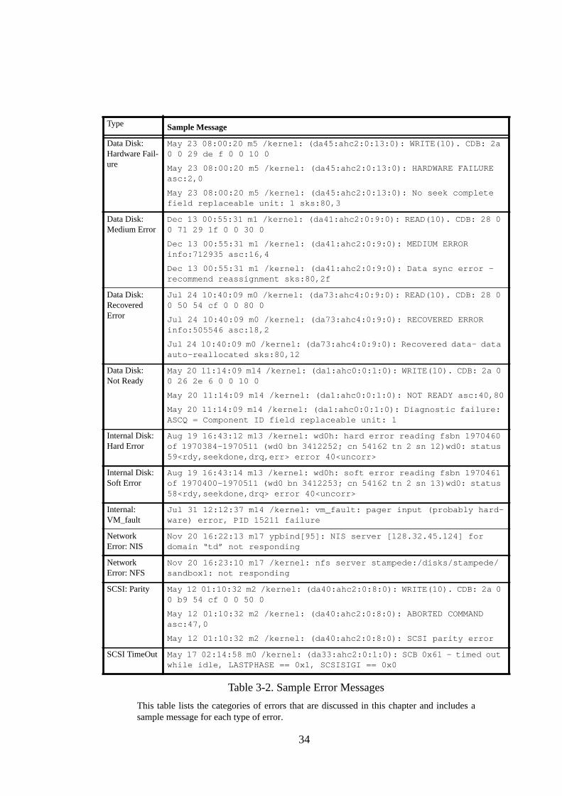
34
Type Sample Message
Data Disk:Hardware Fail-ure
May 23 08:00:20 m5 /kernel: (da45:ahc2:0:13:0): WRITE(10). CDB: 2a0 0 29 de f 0 0 10 0
May 23 08:00:20 m5 /kernel: (da45:ahc2:0:13:0): HARDWARE FAILUREasc:2,0
May 23 08:00:20 m5 /kernel: (da45:ahc2:0:13:0): No seek completefield replaceable unit: 1 sks:80,3
Data Disk:Medium Error
Dec 13 00:55:31 m1 /kernel: (da41:ahc2:0:9:0): READ(10). CDB: 28 00 71 29 1f 0 0 30 0
Dec 13 00:55:31 m1 /kernel: (da41:ahc2:0:9:0): MEDIUM ERRORinfo:712935 asc:16,4
Dec 13 00:55:31 m1 /kernel: (da41:ahc2:0:9:0): Data sync error -recommend reassignment sks:80,2f
Data Disk:RecoveredError
Jul 24 10:40:09 m0 /kernel: (da73:ahc4:0:9:0): READ(10). CDB: 28 00 50 54 cf 0 0 80 0
Jul 24 10:40:09 m0 /kernel: (da73:ahc4:0:9:0): RECOVERED ERRORinfo:505546 asc:18,2
Jul 24 10:40:09 m0 /kernel: (da73:ahc4:0:9:0): Recovered data- dataauto-reallocated sks:80,12
Data Disk:Not Ready
May 20 11:14:09 m14 /kernel: (da1:ahc0:0:1:0): WRITE(10). CDB: 2a 00 26 2e 6 0 0 10 0
May 20 11:14:09 m14 /kernel: (da1:ahc0:0:1:0): NOT READY asc:40,80
May 20 11:14:09 m14 /kernel: (da1:ahc0:0:1:0): Diagnostic failure:ASCQ = Component ID field replaceable unit: 1
Internal Disk:Hard Error
Aug 19 16:43:12 m13 /kernel: wd0h: hard error reading fsbn 1970460of 1970384-1970511 (wd0 bn 3412252; cn 54162 tn 2 sn 12)wd0: status59<rdy,seekdone,drq,err> error 40<uncorr>
Internal Disk:Soft Error
Aug 19 16:43:14 m13 /kernel: wd0h: soft error reading fsbn 1970461of 1970400-1970511 (wd0 bn 3412253; cn 54162 tn 2 sn 13)wd0: status58<rdy,seekdone,drq> error 40<uncorr>
Internal:VM_fault
Jul 31 12:12:37 m14 /kernel: vm_fault: pager input (probably hard-ware) error, PID 15211 failure
NetworkError: NIS
Nov 20 16:22:13 m17 ypbind[95]: NIS server [128.32.45.124] fordomain “td” not responding
NetworkError: NFS
Nov 20 16:23:10 m17 /kernel: nfs server stampede:/disks/stampede/sandbox1: not responding
SCSI: Parity May 12 01:10:32 m2 /kernel: (da40:ahc2:0:8:0): WRITE(10). CDB: 2a 00 b9 54 cf 0 0 50 0
May 12 01:10:32 m2 /kernel: (da40:ahc2:0:8:0): ABORTED COMMANDasc:47,0
May 12 01:10:32 m2 /kernel: (da40:ahc2:0:8:0): SCSI parity error
SCSI TimeOut May 17 02:14:58 m0 /kernel: (da33:ahc2:0:1:0): SCB 0x61 - timed outwhile idle, LASTPHASE == 0x1, SCSISIGI == 0x0
Table 3-2. Sample Error Messages
This table lists the categories of errors that are discussed in this chapter and includes asample message for each type of error.
35
The Hardware Failure message indicates that the command terminated (unsuc-
cessfully) due to a non-recoverable hardware failure. The first and third lines
describe the type of failure that occurred.
The Medium Error indicates that the operation was unsuccessful due to a flaw in
the medium. In this case, the third line recommends that some sectors be re-
assigned. The line between Hardware Failures and Medium Errors is blurry; it is
possible for a drive to report a flaw in the medium as a Hardware Failure [SCSI2].
A Recovered Error indicates that the last command completed with the help of
some error recovery at the target. This happens, for instance, if a bad sector is dis-
covered. Drives handle bad sectors by dynamically re-assigning the affected
sector to an available spare sector [Worthington95, Schwarderer96]. The table
shows such an instance. If more than one recoverable error occurs within a single
request, the drive chooses which error to report. Finally, A Not Ready message
means that the drive is unprepared to serve requests.
2. Internal Disk Errors
The internal disks are IDE Drives. The logs contained two types of errors for IDE
drives: soft errors and hard errors. Unlike the SCSI disk errors, these messages are
operating system specific. By examining the operating system source code, we
learned that soft errors were operations that encountered some form of error but
recovered, while hard errors were operations that were not successful after the
maximum number of retries. The request information is buried within the error
36
message; for instance, the hard error message listed in Table 3-2 occurred while
the drive was trying to read block number 1970460.
3. Internal vm_fault
This error message appears when the OS kernel attempts to read a page into vir-
tual memory for a process. The error indicates that the read needed to satisfy the
page fault did not complete successfully. This error usually causes the affected
process to terminate abnormally.
4. Network Errors
Our system reported two types of network errors, those related to the naming
(NIS) services and those related to network file system (NFS) services. These
errors were reported whenever the system was unable to contact one of these ser-
vices (i.e., the problem was not in the reporting machine).
5. SCSI Errors
The two SCSI errors are TimeOuts and Parity errors; both are self explanatory.
SCSI Timeouts can happen in any of the SCSI bus phases. In our analysis, we
don’t separate the SCSI Timeout errors by SCSI BUS phase. By inspecting the
OS source, we found that the SCSI driver usually responds to a SCSI timeout by
issuing a BUS RESET command. This operation aborts all outstanding com-
mands on the SCSI bus. The other type of SCSI error is Parity. As Table 3.2
shows, SCSI parity error messages appear as the cause of an aborted request.
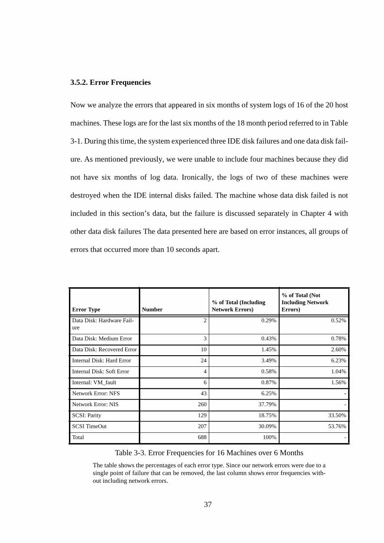
37
3.5.2. Error Frequencies
Now we analyze the errors that appeared in six months of system logs of 16 of the 20 host
machines. These logs are for the last six months of the 18 month period referred to in Table
3-1. During this time, the system experienced three IDE disk failures and one data disk fail-
ure. As mentioned previously, we were unable to include four machines because they did
not have six months of log data. Ironically, the logs of two of these machines were
destroyed when the IDE internal disks failed. The machine whose data disk failed is not
included in this section’s data, but the failure is discussed separately in Chapter 4 with
other data disk failures The data presented here are based on error instances, all groups of
errors that occurred more than 10 seconds apart.
Error Type Number% of Total (IncludingNetwork Errors)
% of Total (NotIncluding NetworkErrors)
Data Disk: Hardware Fail-ure
2 0.29% 0.52%
Data Disk: Medium Error 3 0.43% 0.78%
Data Disk: Recovered Error 10 1.45% 2.60%
Internal Disk: Hard Error 24 3.49% 6.23%
Internal Disk: Soft Error 4 0.58% 1.04%
Internal: VM_fault 6 0.87% 1.56%
Network Error: NFS 43 6.25% -
Network Error: NIS 260 37.79% -
SCSI: Parity 129 18.75% 33.50%
SCSI TimeOut 207 30.09% 53.76%
Total 688 100% -
Table 3-3. Error Frequencies for 16 Machines over 6 Months
The table shows the percentages of each error type. Since our network errors were due to asingle point of failure that can be removed, the last column shows error frequencies with-out including network errors.
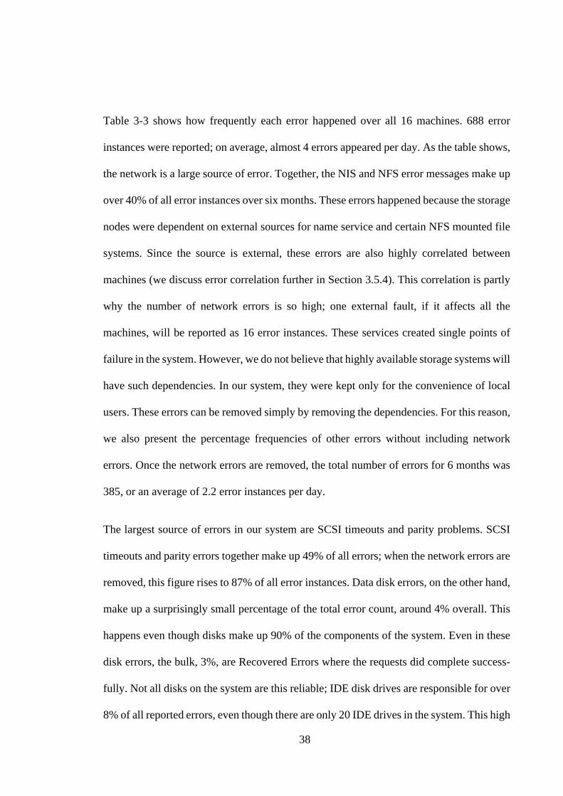
38
Table 3-3 shows how frequently each error happened over all 16 machines. 688 error
instances were reported; on average, almost 4 errors appeared per day. As the table shows,
the network is a large source of error. Together, the NIS and NFS error messages make up
over 40% of all error instances over six months. These errors happened because the storage
nodes were dependent on external sources for name service and certain NFS mounted file
systems. Since the source is external, these errors are also highly correlated between
machines (we discuss error correlation further in Section 3.5.4). This correlation is partly
why the number of network errors is so high; one external fault, if it affects all the
machines, will be reported as 16 error instances. These services created single points of
failure in the system. However, we do not believe that highly available storage systems will
have such dependencies. In our system, they were kept only for the convenience of local
users. These errors can be removed simply by removing the dependencies. For this reason,
we also present the percentage frequencies of other errors without including network
errors. Once the network errors are removed, the total number of errors for 6 months was
385, or an average of 2.2 error instances per day.
The largest source of errors in our system are SCSI timeouts and parity problems. SCSI
timeouts and parity errors together make up 49% of all errors; when the network errors are
removed, this figure rises to 87% of all error instances. Data disk errors, on the other hand,
make up a surprisingly small percentage of the total error count, around 4% overall. This
happens even though disks make up 90% of the components of the system. Even in these
disk errors, the bulk, 3%, are Recovered Errors where the requests did complete success-
fully. Not all disks on the system are this reliable; IDE disk drives are responsible for over
8% of all reported errors, even though there are only 20 IDE drives in the system. This high

39
count of IDE errors is partly due to a failed IDE disk in machine 8. For the most part, the
error percentages match the failure rates in Table 3-1; SCSI bus failures on enclosures and
IDE drive failures make up the bulk of the absolute failures on the system.
Next we break the error information down by machine. Figure 3-2 shows the categories of
errors that each machine experienced. Note that Figure 3-2 does not show the total number
of errors reported on each machine; that data is in the accompanying table, Table 3-4. Not
surprisingly, all machines had a share of network errors. Figure 3-2 shows that IDE disk
errors actually appeared on only 3 machines, machines 5, 8 and 13. Data disk errors also
appeared on 8 machines. The figure also shows that 11 of the 16 machines experienced
SCSI timeout errors.
Table 3-4 shows that the error frequencies vary widely between machines. Ten machines
reported between 10 to 30 error instances, while three of the machines reported over 90
errors in the same time frame. Machines 1, 3 and 7 reported the most errors. Figure 3 shows
that, in all three cases, the bulk of the messages were all in a single category; for machines
1 and 7 the category was SCSI timeout, while for machine 3 it was SCSI parity. This data
suggests an impending failure or other serious problem in each machine. We were able to
trace the parity errors in machine 3 to an enclosure replacement that happened later. There
were no SCSI component replacements in machines 1 and 7; this suggests that the problem
may have been a loose cable that was later fixed. The SCSI errors in machine 9 also led to
a later cable replacement. The only other component replacement that occurred during the
six months was the IDE drive on machine 8.
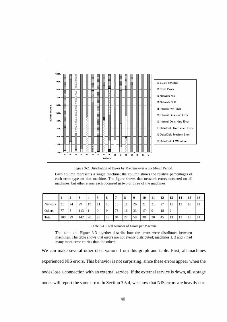
40
We can make several other observations from this graph and table. First, all machines
experienced NIS errors. This behavior is not surprising, since these errors appear when the
nodes lose a connection with an external service. If the external service is down, all storage
nodes will report the same error. In Section 3.5.4, we show that NIS errors are heavily cor-
Figure 3-2. Distribution of Errors by Machine over a Six Month Period.
Each column represents a single machine; the column shows the relative percentages ofeach error type on that machine. The figure shows that network errors occurred on allmachines, but other errors each occurred in two or three of the machines.
1 2 3 4 5 6 7 8 9 10 11 12 13 14 15 16
Network 31 24 29 19 11 10 18 11 26 21 21 27 11 12 18 14
Others 77 5 113 1 9 9 76 16 33 17 9 18 2 - - -
Total 108 29 142 20 20 19 94 27 59 38 30 45 13 12 18 14
Table 3-4. Total Number of Errors per Machine
This table and Figure 3-3 together describe how the errors were distributed betweenmachines. The table shows that errors are not evenly distributed; machines 1, 3 and 7 hadmany more error entries than the others.
41
related between machines. The other type of network error, NFS, does not occur on all
machines. This happened because not all machines were mounting the same NFS filesys-
tems at the same time. Second, 10 of the 16 machines reported SCSI timeouts. In this case,
the cause was not external; the SCSI subsystems of the machines are independent of each
other. Also, the number of SCSI timeouts is not correlated with the number of disks on a
node; node 7 has a large number of timeouts even though it only hosts 16 disks. Finally,
although Table 3-3 shows that SCSI parity errors have high frequency, Figure 3-2 shows
that almost all of these errors appeared on a single machine, caused by an enclosure failure.
Even though the number of potential problems on a system this large is virtually unlimited,
only ten different types of problems occurred over the six months. Another interesting
observation is that no type of error was limited to only one machine. SCSI, IDE disk and
other errors all occurred on at least two machines. This distribution suggests that even
though many combinations of errors can occur in theory on a storage system, there are a
small set of problems that can be expected to occur in a given architecture. We can also
conjecture that if an error happens once, it may happen again on a different machine.
3.5.3. Analysis of Reboots
The prior section looked at the errors that appeared in six months of system logs. The real
question is though, what are the consequences of these errors? To address this question, we
looked at restarts of nodes in the prototype. For each restart that occurred, we checked the
prior 24 hours of the system log for any errors that could be related to the shutdown. We

42
used these errors to guess the reason for the restart. After studying the causes of restarts,
we classified the restarts into the following four categories:
Cold Boot: A Cold Boot is a reboot that occurred without an explicit shutdown or
reboot command. All reboots or shutdown commands leave an entry in the system
log. When no such entry is present, we assume that the machine was power cycled,
either intentionally or because of a power outage. Normally, a machine will not be
power cycled unless all attempts to login via network or serial port have failed.
Reboot: A reboot is a restart of a machine with a prior reboot or shutdown com-
mand.
Within Maintenance Reboot: This is a reboot that happened within 3 hours of a prior
reboot. In this case, we assume that both reboots are part of the same maintenance
session.
For Schedulable Maintenance: If an explicit shutdown occurs without any error
messages within the prior 24 hours, we assume that the shutdown was for a planned
maintenance activity, such as a hardware replacement or upgrade. We call this cat-
egory Schedulable because we assume that the shutdown could have been moved
to another time.
Table 3-5 shows the number of times that each machine was restarted, and Figure 3-3
shows the percentages of restarts from each category for each machine. This data does not
include Within-Maintenance Reboots, since we consider them to have happened while the
node was down. Overall, we found that all machines were restarted at least twice in the six
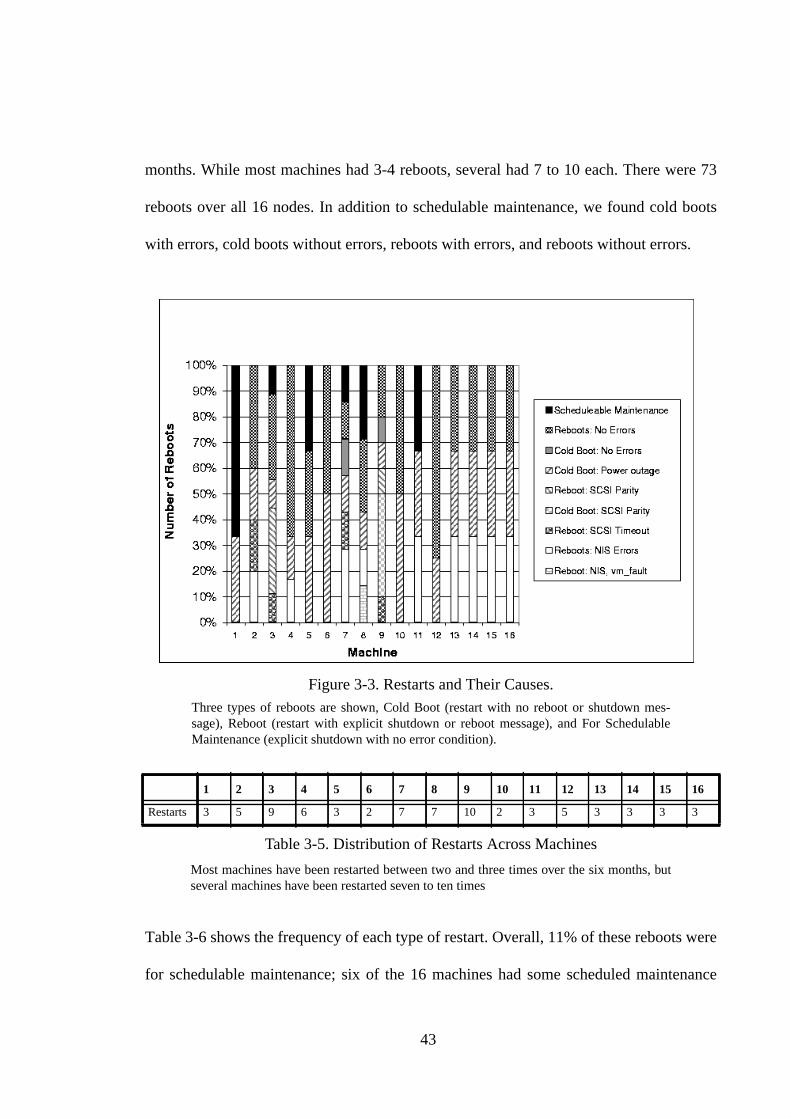
43
months. While most machines had 3-4 reboots, several had 7 to 10 each. There were 73
reboots over all 16 nodes. In addition to schedulable maintenance, we found cold boots
with errors, cold boots without errors, reboots with errors, and reboots without errors.
Table 3-6 shows the frequency of each type of restart. Overall, 11% of these reboots were
for schedulable maintenance; six of the 16 machines had some scheduled maintenance
Figure 3-3. Restarts and Their Causes.Three types of reboots are shown, Cold Boot (restart with no reboot or shutdown mes-sage), Reboot (restart with explicit shutdown or reboot message), and For SchedulableMaintenance (explicit shutdown with no error condition).
1 2 3 4 5 6 7 8 9 10 11 12 13 14 15 16
Restarts 3 5 9 6 3 2 7 7 10 2 3 5 3 3 3 3
Table 3-5. Distribution of Restarts Across Machines
Most machines have been restarted between two and three times over the six months, butseveral machines have been restarted seven to ten times

44
done on them. A single power outage accounts for 22% of all restarts. Another 33% were
explicit reboots with no errors in the log; these reboots could have been for software main-
tenance. It is very unlikely that a machine was explicitly rebooted for no good reason, how-
ever, we cannot tell from the system logs whether a software upgrade took place. All
machines were rebooted without errors. Two machines also received cold boots with no
error messages. Finally, the remaining 32% of restarts happened due to errors.
We found only three types of error instances that preceded reboots or cold boots; they were
SCSI Timeout, SCSI parity, and NIS errors. Two machines were restarted for SCSI parity
problems; one of these is machine 3 that had the failed disk enclosure. Four machines were
restarted for SCSI timeout problems. By far, the main cause of reboots and cold boots was
NIS errors. All the machines but one were restarted because of network problems. The
reason could be that network errors are more fatal to an OS than SCSI errors. While the
effects of SCSI errors can be limited to the processes that are reading or writing to the
affected drives, the network errors affect all communication between the machine and the
outside world.
Restart Type Number % of Total
Schedulable Maintenance 8 11.0%
Reboot: No Errors 24 32.9%
Reboot: Errors 19 26.0%
Cold Boot: No Errors 2 2.7%
Cold Boot: Errors 4 5.5%
Power Outage 16 21.9%
Table 3-6. Frequency of Each Type of Restart
The table lists breaks the Reboot and Cold Boot categories into two subcategories, thosewith errors and without errors. A Reboot with errors is an instance where the log datashowed errors before the explicit reboot. A Cold Boot with errors is a case where the logdata showed a restart, without an explicit reboot, and errors appeared before the restartoccurred. As such, a Cold Boot without errors is a very unlikely occurrence.

45
One interesting point is that no machine restarts happened because of data disk or IDE disk
errors. Even though there were hard errors on the three of the 16 system disks, these errors
did not cause the operating system to crash. The OS survived hard errors on the internal
disk because all of the errors occurred on a user partition that occupied around 80% of the
drive.
3.5.4. Correlations
Sections 3.5.2 and 3.5.3 described aggregate data on types of errors and causes of reboots.
In this section we examine the time correlation between errors, within and between
machines.
Figures 3-4 and 3-5 show the time distribution of errors. The X axis is time and the Y axis
shows the identification numbers of each machine. The errors for each machine over time
appear on a single horizontal line. A vertical line indicates correlation of errors between
machines. Figure 3-4 only shows NFS and NIS errors, while Figure 3-5 shows all other
errors. It is clear from Figure 3-4 that network errors are correlated between machines. This
data reiterates the need to remove all single points of failure from a highly available storage
system. The bulk of the errors are NIS errors. When NFS errors occur, they also seem to
be correlated with NIS errors.
Figure 3-5 shows all other forms of errors. In this case there is no reason to expect errors
on different machines to be correlated; each node is relatively independent of all other
nodes. However, the figure shows that even though there is no direct correlation between
SCSI errors (no single source), it is possible to have several SCSI errors across different
machines at the same time. For example, near August 13, 1998, several machines experi-
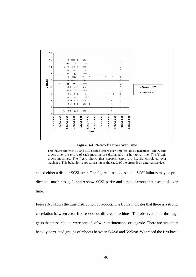
46
enced either a disk or SCSI error. The figure also suggests that SCSI failures may be pre-
dictable; machines 1, 3, and 9 show SCSI parity and timeout errors that escalated over
time.
Figure 3-6 shows the time distribution of reboots. The figure indicates that there is a strong
correlation between error-free reboots on different machines. This observation further sug-
gests that these reboots were part of software maintenance or upgrade. There are two other
heavily correlated groups of reboots between 5/5/98 and 5/25/98. We traced the first back
Figure 3-4. Network Errors over TimeThis figure shows NFS and NIS related errors over time for all 16 machines. The X axisshows time; the errors of each machine are displayed on a horizontal line. The Y axisshows machines. The figure shows that network errors are heavily correlated overmachines. This behavior is not surprising as the cause of the errors is an external service.
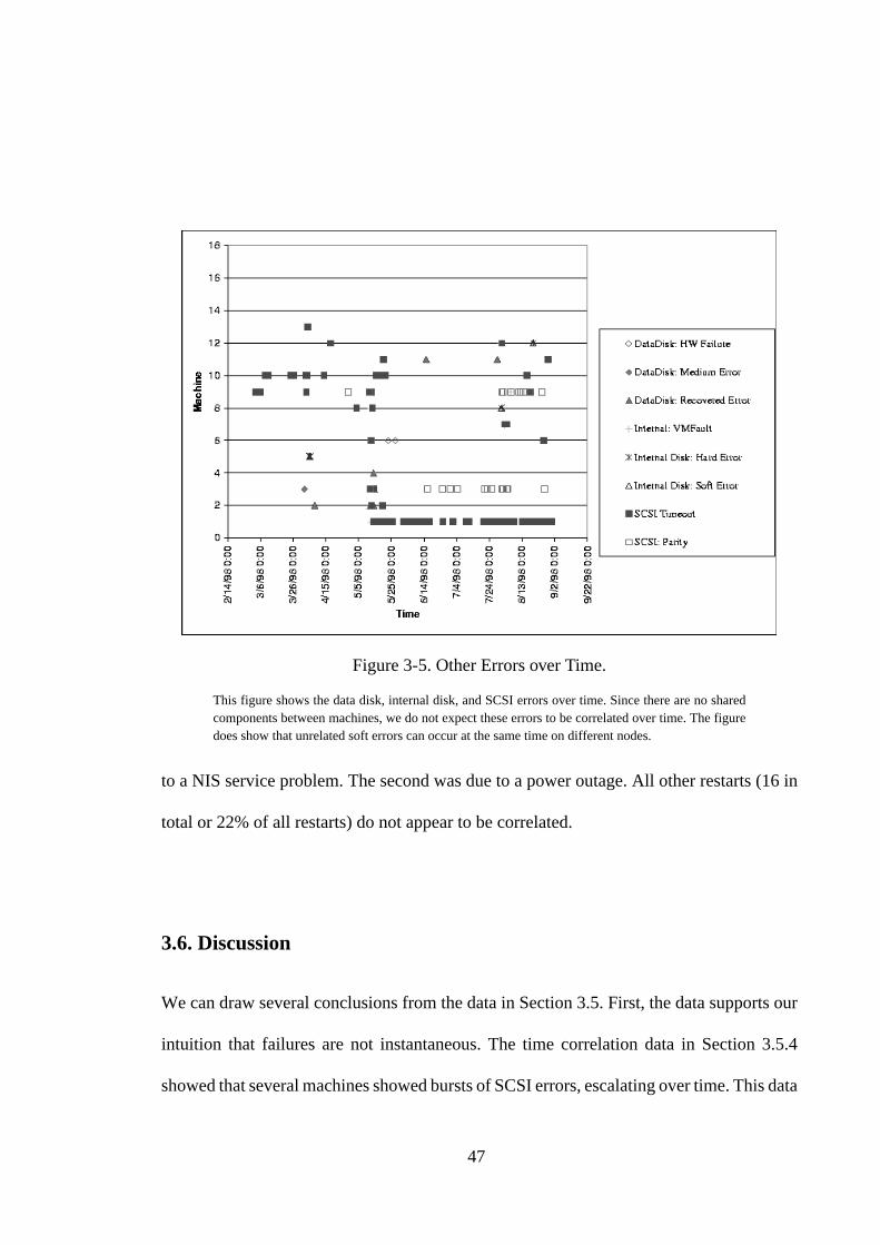
47
to a NIS service problem. The second was due to a power outage. All other restarts (16 in
total or 22% of all restarts) do not appear to be correlated.
3.6. Discussion
We can draw several conclusions from the data in Section 3.5. First, the data supports our
intuition that failures are not instantaneous. The time correlation data in Section 3.5.4
showed that several machines showed bursts of SCSI errors, escalating over time. This data
Figure 3-5. Other Errors over Time.
This figure shows the data disk, internal disk, and SCSI errors over time. Since there are no sharedcomponents between machines, we do not expect these errors to be correlated over time. The figuredoes show that unrelated soft errors can occur at the same time on different nodes.
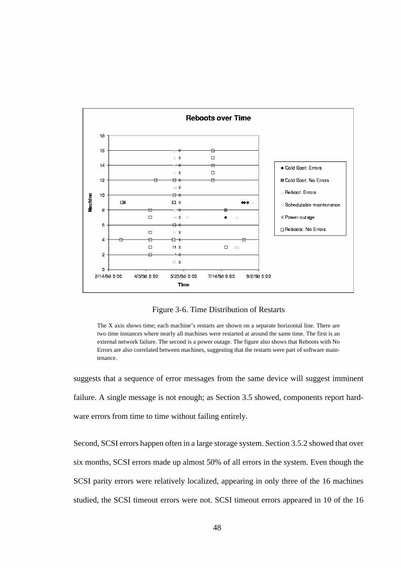
48
suggests that a sequence of error messages from the same device will suggest imminent
failure. A single message is not enough; as Section 3.5 showed, components report hard-
ware errors from time to time without failing entirely.
Second, SCSI errors happen often in a large storage system. Section 3.5.2 showed that over
six months, SCSI errors made up almost 50% of all errors in the system. Even though the
SCSI parity errors were relatively localized, appearing in only three of the 16 machines
studied, the SCSI timeout errors were not. SCSI timeout errors appeared in 10 of the 16
Figure 3-6. Time Distribution of Restarts
The X axis shows time; each machine’s restarts are shown on a separate horizontal line. There aretwo time instances where nearly all machines were restarted at around the same time. The first is anexternal network failure. The second is a power outage. The figure also shows that Reboots with NoErrors are also correlated between machines, suggesting that the restarts were part of software main-tenance.
49
machines. These timeouts affect system performance for two reasons. First, a timeout typ-
ically indicates that devices that wish to use the bus are not able to use it, delaying requests.
Second, as the SCSI controller regains control by issuing a BUS RESET, a timeout can
cause the controller to abort all active requests on the bus. When there a large number of
disks on the bus and each disk has several tagged commands outstanding, a SCSI timeout
can severely degrade performance. The data also suggests that failures of SCSI compo-
nents are predictable. Disks already provide some warning that failure is imminent; the
data in Sections 3.5.2 and 3.5.4 suggest that SCSI failures may also be predictable. Since
many disks are dependent on a single SCSI bus, it would be very useful to predict the fail-
ures of SCSI buses. It may also be possible to avoid the degraded performance that occurs
before a SCSI bus has an absolute failure.
Third, the data also shows that data disks are among the most reliable components in the
system. Section 3.3 showed that data disks had the lowest percentage failure rate of all
components that failed in one year. This data suggests that work in the literature that has
focused on disk reliability [Burkhard93, Ng94] do not adequately reflect the reliability
challenges of real systems.
3.7. Summary
This chapter presented an analysis of hardware errors in a large storage system. We show
results from six months of system logs on 16 machines, absolute failure data for the entire
prototype for eighteen months, and four case studies of disk drive failures. The data
50
showed that data drives are among the most reliable components in the system, while SCSI
components generated a considerable number of errors. The data shows that no failure hap-
pens instantly, and that there are performance consequences when operating with degraded
components.
The data also supported the idea that it is possible to predict the failure of both disk drives
and SCSI components. The next chapter explores this idea in more depth. In particular, we
analyze error streams that occur before SCSI and disk drive failures to determine the long
term characteristics of failure events. Chapter 4 also explores the effectiveness of predic-
tion techniques to detect and remove failing components before they can degrade the
system performance and availability.
51
4 Characterizing Failures
4.1. Introduction
This chapter explores the failure behavior of devices in depth. In particular, we attempt to
understand what outward signs accompany the failure of disks and SCSI systems. We
present cases of device failure; for each case we ask the following questions: what mes-
sages appear before failure?, can these messages be used to predict failure?, how do the
messages compare in type to what appears without a failure? and finally, can all this infor-
mation be used to determine the best cause for action when a failure occurs? We also
present some evidence of the side effects of failures.
Section 4.2 defines different types of failure events. The terms defined are used in the dis-
cussions of failures in the rest of the chapter. The remainder of the chapter focuses on
understanding the nature of SCSI and disk drive failures. To do this, we begin by present-
ing each failure case for which system logs are available. For each case, we determine the
type of messages that were reported and whether those messages increased in intensity
over time. The next section, section 4.4, determines whether these failures are predictable
by applying a failure prediction algorithm. Section 4.5 presents empirical data on the side
effects of disk drive failure and section 4.6 concludes with a summary.

52
4.2. Methodology
Before we explore the nature of failures, we must define exactly what is meant by a failure.
The literature uses various terms to define failure events, transient, intermittent and per-
manent faults. Transient faults, as the name implies, are errors that appear and disappear
with no action needed. Intermittent faults tend to reoccur over time. Transient and inter-
mittent faults differ in that intermittent faults can be removed by replacing hardware, while
transient faults cannot. Once the hardware is replaced, the fault is labeled permanent
[Lin90]. The decision to replace hardware is subjective, and is usually made by a system
administrator when a component’s error behavior exceeds some tolerance level. In this the-
sis, such faults are also called absolute or hard failures.
Chapter 3 used the system logs gathered from the prototype to determine the nature of soft
failures. This chapter uses the same logs to study the nature of absolute (or hard) failures.
As Figure 3-1 in Chapter 3 showed, each error message identifies the device or subsystem
that is reporting the error. Using this information, we can separate the log data into per-
device error streams. Studying the error streams of failing devices and comparing them
with error streams of other devices reveals the nature of failures.
In addition to the types of failure outlined above, we define an extra category of errors,
Required Human Intervention. The error data presented so far showed that recurring errors
are far more common than hardware replacement. In quite a few cases, a problem that gen-
erated a series of recurring errors was solved by a hard or soft system reset. This type of
problem is not transient, since the errors do not disappear with no intervention, and cannot
be termed permanent or absolute since no hardware is replaced. We define such problems

53
as requiring human intervention. The system logs show cases where humans intervened.
In particular, if the host machine was manually shutdown or rebooted several times before
the error stream stopped, we assume human intervention.
4.3. A Look At Failure Cases
This section takes a more in-depth look at the failure cases of SCSI and disk drive compo-
nents. SCSI failures deserve an in-depth look because the soft error data presented in Chap-
ter 3 revealed that SCSI errors made up the largest percentage of all errors experienced by
the system. Also it would be particularly useful to predict SCSI bus failures since they
affect many disk drives. It is important to understand data disk failures since the data disks
are the most numerous and the most important part of any storage system.
We present each failure case in turn and describe both the types of messages that preceded
the failure event, and the duration of messages.
4.3.1. SCSI Cases
There were three SCSI bus failure cases for which system log data was available; Table 4-
1 summarizes the cases. For each case, the table shows the types of messages that occurred,
the number of messages and the duration of messages. As the table shows, all three SCSI
failures displayed Parity error messages. Two of the three cases displayed Timeout mes-
sages as well. The first and third case displayed considerably more messages than the
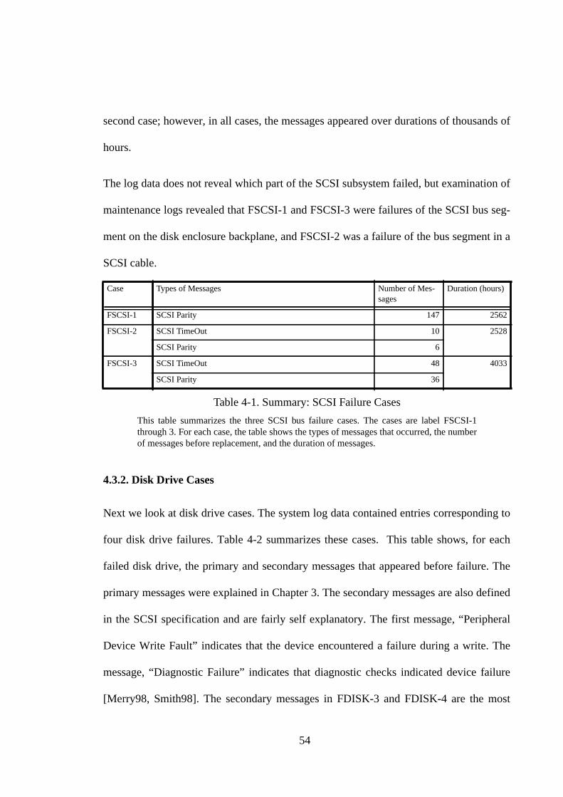
54
second case; however, in all cases, the messages appeared over durations of thousands of
hours.
The log data does not reveal which part of the SCSI subsystem failed, but examination of
maintenance logs revealed that FSCSI-1 and FSCSI-3 were failures of the SCSI bus seg-
ment on the disk enclosure backplane, and FSCSI-2 was a failure of the bus segment in a
SCSI cable.
4.3.2. Disk Drive Cases
Next we look at disk drive cases. The system log data contained entries corresponding to
four disk drive failures. Table 4-2 summarizes these cases. This table shows, for each
failed disk drive, the primary and secondary messages that appeared before failure. The
primary messages were explained in Chapter 3. The secondary messages are also defined
in the SCSI specification and are fairly self explanatory. The first message, “Peripheral
Device Write Fault” indicates that the device encountered a failure during a write. The
message, “Diagnostic Failure” indicates that diagnostic checks indicated device failure
[Merry98, Smith98]. The secondary messages in FDISK-3 and FDISK-4 are the most
Case Types of Messages Number of Mes-sages
Duration (hours)
FSCSI-1 SCSI Parity 147 2562
FSCSI-2 SCSI TimeOut 10 2528
SCSI Parity 6
FSCSI-3 SCSI TimeOut 48 4033
SCSI Parity 36
Table 4-1. Summary: SCSI Failure Cases
This table summarizes the three SCSI bus failure cases. The cases are label FSCSI-1through 3. For each case, the table shows the types of messages that occurred, the numberof messages before replacement, and the duration of messages.
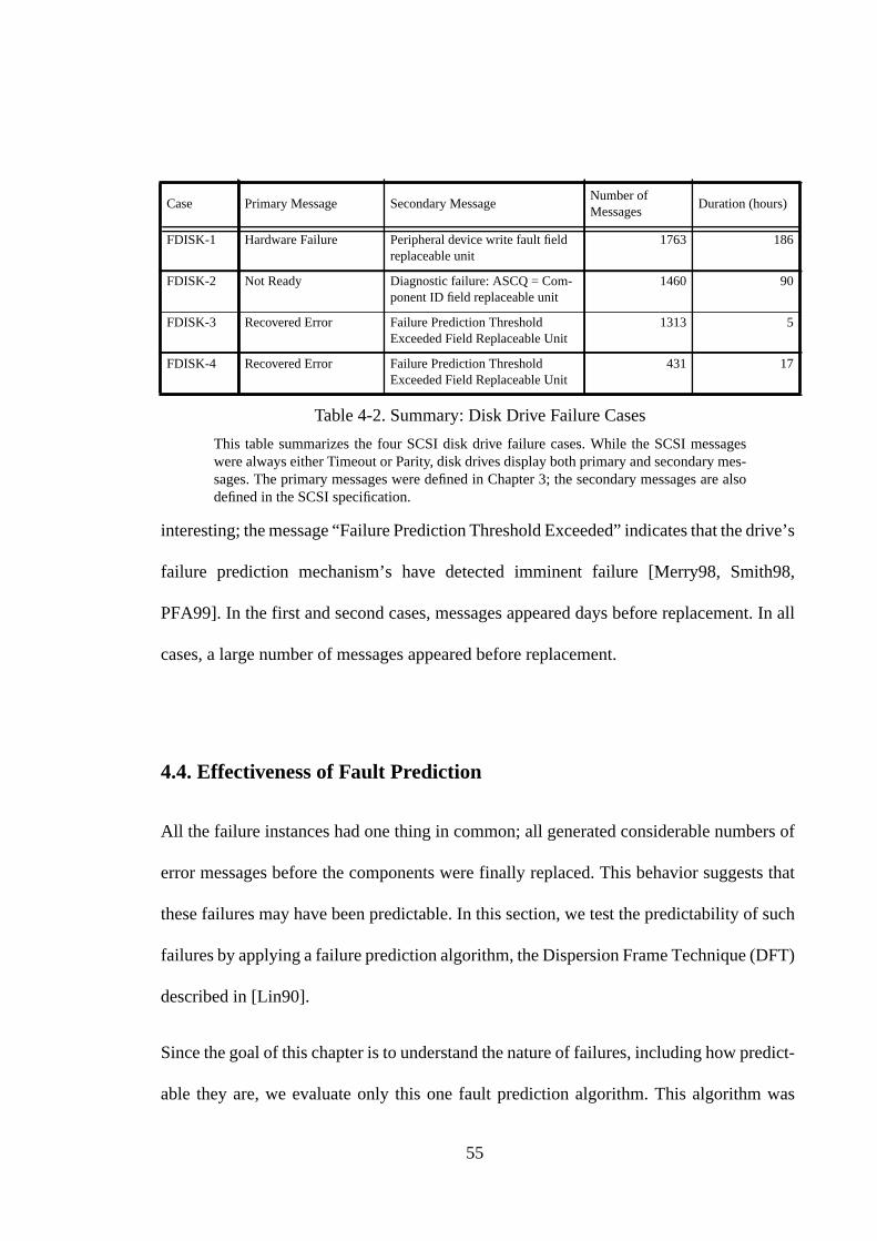
55
interesting; the message “Failure Prediction Threshold Exceeded” indicates that the drive’s
failure prediction mechanism’s have detected imminent failure [Merry98, Smith98,
PFA99]. In the first and second cases, messages appeared days before replacement. In all
cases, a large number of messages appeared before replacement.
4.4. Effectiveness of Fault Prediction
All the failure instances had one thing in common; all generated considerable numbers of
error messages before the components were finally replaced. This behavior suggests that
these failures may have been predictable. In this section, we test the predictability of such
failures by applying a failure prediction algorithm, the Dispersion Frame Technique (DFT)
described in [Lin90].
Since the goal of this chapter is to understand the nature of failures, including how predict-
able they are, we evaluate only this one fault prediction algorithm. This algorithm was
Case Primary Message Secondary MessageNumber ofMessages
Duration (hours)
FDISK-1 Hardware Failure Peripheral device write fault fieldreplaceable unit
1763 186
FDISK-2 Not Ready Diagnostic failure: ASCQ = Com-ponent ID field replaceable unit
1460 90
FDISK-3 Recovered Error Failure Prediction ThresholdExceeded Field Replaceable Unit
1313 5
FDISK-4 Recovered Error Failure Prediction ThresholdExceeded Field Replaceable Unit
431 17
Table 4-2. Summary: Disk Drive Failure Cases
This table summarizes the four SCSI disk drive failure cases. While the SCSI messageswere always either Timeout or Parity, disk drives display both primary and secondary mes-sages. The primary messages were defined in Chapter 3; the secondary messages are alsodefined in the SCSI specification.
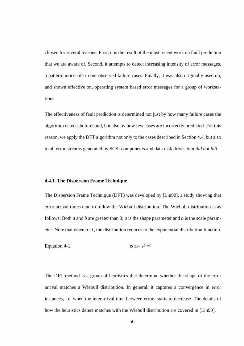
56
chosen for several reasons. First, it is the result of the most recent work on fault prediction
that we are aware of. Second, it attempts to detect increasing intensity of error messages,
a pattern noticeable in our observed failure cases. Finally, it was also originally used on,
and shown effective on, operating system based error messages for a group of worksta-
tions.
The effectiveness of fault prediction is determined not just by how many failure cases the
algorithm detects beforehand, but also by how few cases are incorrectly predicted. For this
reason, we apply the DFT algorithm not only to the cases described in Section 4.4, but also
to all error streams generated by SCSI components and data disk drivesthat did not fail.
4.4.1. The Dispersion Frame Technique
The Dispersion Frame Technique (DFT) was developed by [Lin90], a study showing that
error arrival times tend to follow the Wiebull distribution. The Wiebull distribution is as
follows: Botha andb are greater than 0;a is the shape parameter andb is the scale param-
eter. Note that whena=1, the distribution reduces to the exponential distribution function.
Equation 4-1.
The DFT method is a group of heuristics that determine whether the shape of the error
arrival matches a Wiebull distribution. In general, it captures a convergence in error
instances, i.e. when the interarrival time between errors starts to decrease. The details of
how the heuristics detect matches with the Wiebull distribution are covered in [Lin90].
R t( ) e bt–( )a=
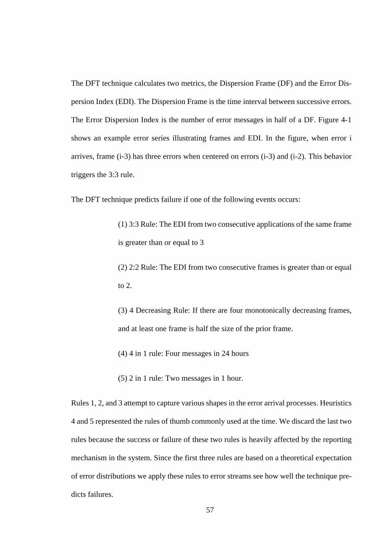
57
The DFT technique calculates two metrics, the Dispersion Frame (DF) and the Error Dis-
persion Index (EDI). The Dispersion Frame is the time interval between successive errors.
The Error Dispersion Index is the number of error messages in half of a DF. Figure 4-1
shows an example error series illustrating frames and EDI. In the figure, when error i
arrives, frame (i-3) has three errors when centered on errors (i-3) and (i-2). This behavior
triggers the 3:3 rule.
The DFT technique predicts failure if one of the following events occurs:
(1) 3:3 Rule: The EDI from two consecutive applications of the same frame
is greater than or equal to 3
(2) 2:2 Rule: The EDI from two consecutive frames is greater than or equal
to 2.
(3) 4 Decreasing Rule: If there are four monotonically decreasing frames,
and at least one frame is half the size of the prior frame.
(4) 4 in 1 rule: Four messages in 24 hours
(5) 2 in 1 rule: Two messages in 1 hour.
Rules 1, 2, and 3 attempt to capture various shapes in the error arrival processes. Heuristics
4 and 5 represented the rules of thumb commonly used at the time. We discard the last two
rules because the success or failure of these two rules is heavily affected by the reporting
mechanism in the system. Since the first three rules are based on a theoretical expectation
of error distributions we apply these rules to error streams see how well the technique pre-
dicts failures.
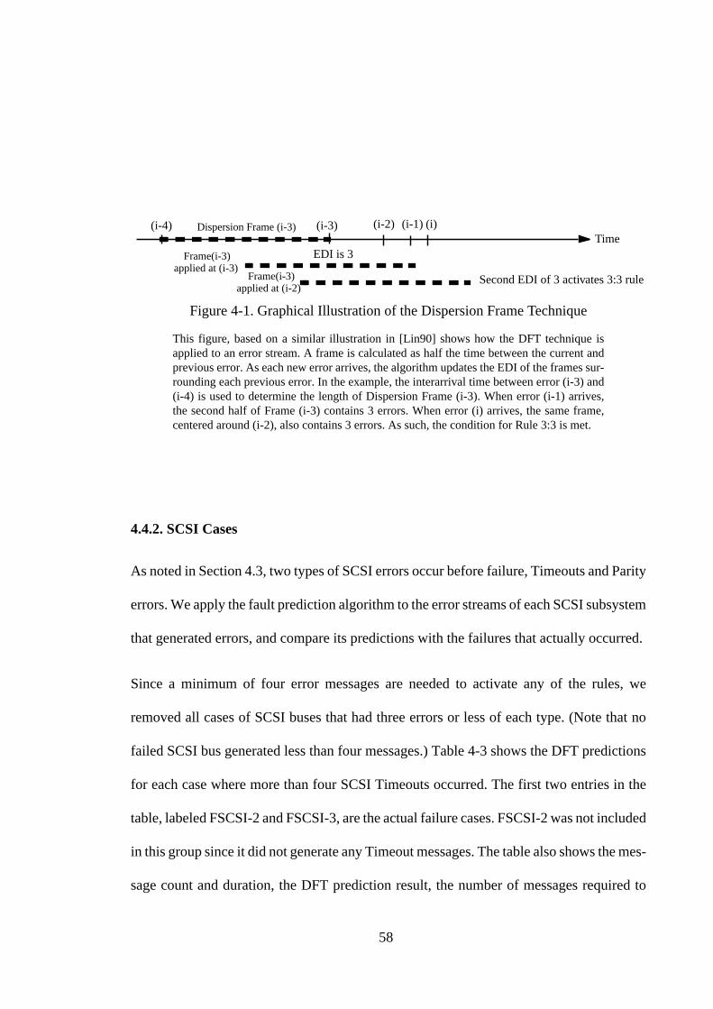
58
4.4.2. SCSI Cases
As noted in Section 4.3, two types of SCSI errors occur before failure, Timeouts and Parity
errors. We apply the fault prediction algorithm to the error streams of each SCSI subsystem
that generated errors, and compare its predictions with the failures that actually occurred.
Since a minimum of four error messages are needed to activate any of the rules, we
removed all cases of SCSI buses that had three errors or less of each type. (Note that no
failed SCSI bus generated less than four messages.) Table 4-3 shows the DFT predictions
for each case where more than four SCSI Timeouts occurred. The first two entries in the
table, labeled FSCSI-2 and FSCSI-3, are the actual failure cases. FSCSI-2 was not included
in this group since it did not generate any Timeout messages. The table also shows the mes-
sage count and duration, the DFT prediction result, the number of messages required to
Figure 4-1. Graphical Illustration of the Dispersion Frame Technique
This figure, based on a similar illustration in [Lin90] shows how the DFT technique isapplied to an error stream. A frame is calculated as half the time between the current andprevious error. As each new error arrives, the algorithm updates the EDI of the frames sur-rounding each previous error. In the example, the interarrival time between error (i-3) and(i-4) is used to determine the length of Dispersion Frame (i-3). When error (i-1) arrives,the second half of Frame (i-3) contains 3 errors. When error (i) arrives, the same frame,centered around (i-2), also contains 3 errors. As such, the condition for Rule 3:3 is met.
Time(i-4) (i-3) (i-2) (i-1) (i)
EDI is 3
Second EDI of 3 activates 3:3 rule
Frame(i-3)
Dispersion Frame (i-3)
applied at (i-3)Frame(i-3)
applied at (i-2)
59
generate a prediction, and the prediction time. The table also shows which cases required
human intervention.
The DFT algorithm predicted nine failures. For both cases where failure occurred, the algo-
rithm generated a positive prediction in one hour or less. However, the algorithm did have
a high false alarm rate; a positive prediction was given for seven cases where no failure
occurred. Further examination of maintenance data revealed that in one of the seven cases,
a component did fail around the time when the messages were generated; a disk drive
attached to the SCSI bus. This event was evidence that disk failures can extend to errors
on the SCSI bus. For the rest of the components, there was no replacement. It is certainly
possible that these components will fail sometime in the future, however, all information
to date suggests that the algorithm is over conservative.
Another way to estimate effectiveness is to compare the DFT failure predictions with
instances that Required Human Intervention. By this metric the DFT algorithm fares much
better. Of the six positive predictions where no component was replaced, the log data in
four cases showed evidence of human intervention.
Of all the SCSI buses, there were only three that reported parity errors; each reported more
than three messages and each was a failure case. Table 4-4 shows prediction effectiveness
when the Parity error streams are used. As the table shows, two of the three failures were
predicted by DFT. The algorithm did not predict the failure of FSCSI-2. This failure was
predicted, on the other hand, when the algorithm was applied to the Timeout message
stream.
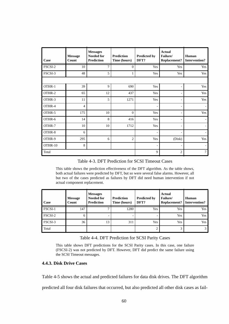
60
4.4.3. Disk Drive Cases
Table 4-5 shows the actual and predicted failures for data disk drives. The DFT algorithm
predicted all four disk failures that occurred, but also predicted all other disk cases as fail-
CaseMessageCount
MessagesNeeded forPrediction
PredictionTime (hours)
Predicted byDFT?
ActualFailure/Replacement?
HumanIntervention?
FSCSI-2 10 7 0 Yes Yes Yes
FSCSI-3 48 5 1 Yes Yes Yes
OTHR-1 39 9 690 Yes - Yes
OTHR-2 65 12 437 Yes - Yes
OTHR-3 11 5 1271 Yes - Yes
OTHR-4 4 - - -
OTHR-5 175 10 0 Yes - Yes
OTHR-6 14 8 416 Yes - -
OTHR-7 10 10 1712 Yes - -
OTHR-8 6 - - -
OTHR-9 295 6 2 Yes (Disk) Yes
OTHR-10 8 - - -
Total 9 2 7
Table 4-3. DFT Prediction for SCSI Timeout Cases
This table shows the prediction effectiveness of the DFT algorithm. As the table shows,both actual failures were predicted by DFT, but so were several false alarms. However, allbut two of the cases predicted as failures by DFT did need human intervention if notactual component replacement.
CaseMessageCount
MessagesNeeded forPrediction
PredictionTime (hours)
Predicted byDFT?
ActualFailure/Replacement?
HumanIntervention?
FSCSI-1 147 7 1280 Yes Yes Yes
FSCSI-2 6 - - - Yes Yes
FSCSI-3 36 13 311 Yes Yes Yes
Total 2 3 3
Table 4-4. DFT Prediction for SCSI Parity Cases
This table shows DFT predictions for the SCSI Parity cases. In this case, one failure(FSCSI-2) was not predicted by DFT. However, DFT did predict the same failure usingthe SCSI Timeout messages.
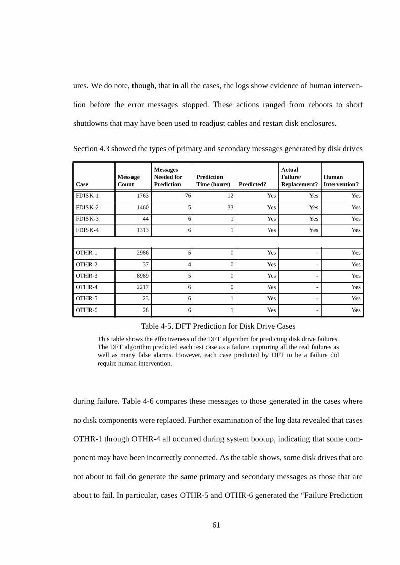
61
ures. We do note, though, that in all the cases, the logs show evidence of human interven-
tion before the error messages stopped. These actions ranged from reboots to short
shutdowns that may have been used to readjust cables and restart disk enclosures.
Section 4.3 showed the types of primary and secondary messages generated by disk drives
during failure. Table 4-6 compares these messages to those generated in the cases where
no disk components were replaced. Further examination of the log data revealed that cases
OTHR-1 through OTHR-4 all occurred during system bootup, indicating that some com-
ponent may have been incorrectly connected. As the table shows, some disk drives that are
not about to fail do generate the same primary and secondary messages as those that are
about to fail. In particular, cases OTHR-5 and OTHR-6 generated the “Failure Prediction
CaseMessageCount
MessagesNeeded forPrediction
PredictionTime (hours) Predicted?
ActualFailure/Replacement?
HumanIntervention?
FDISK-1 1763 76 12 Yes Yes Yes
FDISK-2 1460 5 33 Yes Yes Yes
FDISK-3 44 6 1 Yes Yes Yes
FDISK-4 1313 6 1 Yes Yes Yes
OTHR-1 2986 5 0 Yes - Yes
OTHR-2 37 4 0 Yes - Yes
OTHR-3 8989 5 0 Yes - Yes
OTHR-4 2217 6 0 Yes - Yes
OTHR-5 23 6 1 Yes - Yes
OTHR-6 28 6 1 Yes - Yes
Table 4-5. DFT Prediction for Disk Drive Cases
This table shows the effectiveness of the DFT algorithm for predicting disk drive failures.The DFT algorithm predicted each test case as a failure, capturing all the real failures aswell as many false alarms. However, each case predicted by DFT to be a failure didrequire human intervention.
62
Threshold Exceeded Message”. Further examination of these cases revealed that they were
side effects of the SCSI bus failure FSCSI-2.
4.4.4. Discussion
The close up look at each failure case revealed the following insights:
(i) In all the failure cases that were examined, the devices generated a considerable number
of soft error messages before absolute failure. These messages also tended to increase in
intensity over time. As a result, the DFT algorithm was able to detect all the failure cases
and issue a prediction well before the device was actually replaced.
(ii) Although DFT was good at predicting real failures, it also predicted failure in many
cases where the components were not replaced. These false alarms occurred because other
events also generate many error messages, with more messages as time goes by. Since the
DFT prediction scheme is based entirely on detecting an increasing intensity of error mes-
sages, the algorithm cannot differentiate between these false alarm conditions and actual
failures. However, each case predicted as a failure by DFT did require some form of human
intervention. Therefore, the DFT appears to do better as a detector of cases where human
intervention is needed, rather than a failure prediction algorithm.
(iii) The few SCSI failure cases available for analysis suggest that failing SCSI bus hard-
ware tends to generate both timeout and parity errors. All the false alarm cases generated
timeout errors but none generated parity errors. This observation matches intuition; a fail-
ing SCSI device is likely to have the types of integrity problems that generate parity errors.

63
This distinction may be useful to separate failure cases from the cases that only need
human intervention.
Graph Primary Message Secondary Message
FDISK-1 HARDWARE FAILURE Peripheral device write fault field replaceable unit
FDISK-2 NOT READY Diagnostic failure: ASCQ = Component ID fieldreplaceable unit
FDISK-3 RECOVERED ERROR Failure prediction threshold exceeded field replace-able unit
FDISK-4 RECOVERED ERROR Failure prediction threshold exceeded field replace-able unit
OTHR-1 NOT READY
HARDWARE FAILURE
Logical unit not ready, initializing command requiredInternal target failure field replaceable unit
OTHR-2 NOT READY
HARDWARE FAILURE
Logical unit not ready, initializing command requiredInternal target failure field replaceable unit
OTHR-3 NOT READY
HARDWARE FAILURE
Logical unit not ready, initializing command requiredInternal target failure field replaceable unit
OTHR-4 NOT READY
HARDWARE FAILURE
Logical unit not ready, initializing command requiredInternal target failure field replaceable unit
OTHR-5 RECOVERED ERROR
HARDWARE FAILURE
Failure prediction threshold exceeded field replace-able unit
Diagnostic failure: ASCQ = Component ID fieldreplaceable unit
OTHR-6 RECOVERED ERROR
HARDWARE FAILURE
Failure prediction threshold exceeded field replace-able unitDiagnostic failure: ASCQ = Component ID fieldreplaceable unit
Table 4-6. Primary and Secondary Disk Error Messages
This table compares the primary and secondary messages generated by disks in failureconditions to those generated by disks not in failure conditions. As the table shows, insome cases, drives that are not in failure conditions can generate the same types of mes-sages as those in failure conditions.However, note that these messages appeared on driveconnected to a SCSI bus that failed.
64
(iv) SCSI failures can masquerade as disk failures and vice versa. Table 4-3 shows a case
where a large number of SCSI timeout messages are generated by a failing disk. We exam-
ine this case further in the next section. Table 4-6 shows a case where a single SCSI failure
generated error streams on two disks on the bus.
4.5. Side Effects of Disk Drive Failures
Figure 4-2 shows disk error and SCSI timeout events in one disk failure case. This is the
case labeled FDISK-1 Table 4-2 and the SCSI case labeled OTHR-9 in Table 4-3. The
figure shows that the failing disk generated a large number of SCSI Timeouts. The other
disks on the bus also generated some timeouts. As the intensity of the disk error messages
increased, so did the intensity of the timeout messages.
In this case, the failing disk did interrupt (though it did not halt) the activities of other
devices on the bus. The BSD SCSI driver responds to a SCSI timeout condition by issuing
a BUS RESET command to regain control of the SCSI bus. The BUS RESET has the side
effect of aborting all outstanding commands on the BUS. These commands must be issued
again. Both the timeout and its resulting BUS RESET several handicap the performance of
all devices on the bus. The figure is evidence that it is possible for failing disks to hold on
to the interconnect, causing timeouts and resulting in resets to reclaim the bus.
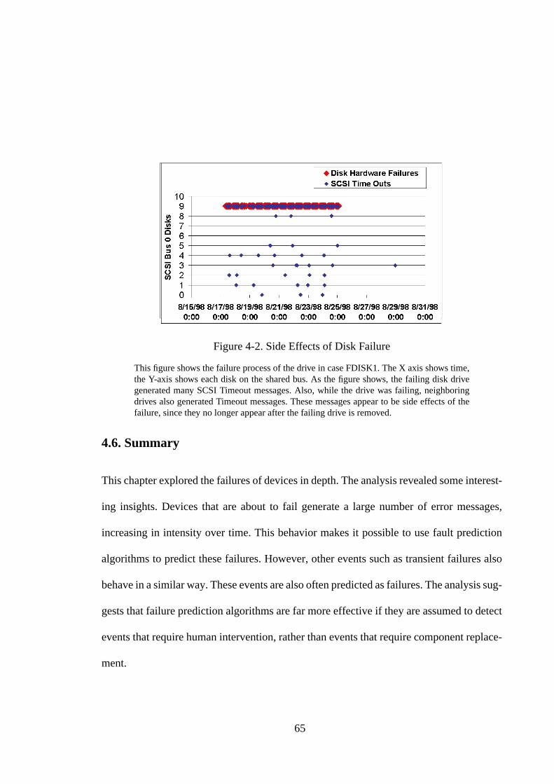
65
4.6. Summary
This chapter explored the failures of devices in depth. The analysis revealed some interest-
ing insights. Devices that are about to fail generate a large number of error messages,
increasing in intensity over time. This behavior makes it possible to use fault prediction
algorithms to predict these failures. However, other events such as transient failures also
behave in a similar way. These events are also often predicted as failures. The analysis sug-
gests that failure prediction algorithms are far more effective if they are assumed to detect
events that require human intervention, rather than events that require component replace-
ment.
Figure 4-2. Side Effects of Disk Failure
This figure shows the failure process of the drive in case FDISK1. The X axis shows time,the Y-axis shows each disk on the shared bus. As the figure shows, the failing disk drivegenerated many SCSI Timeout messages. Also, while the drive was failing, neighboringdrives also generated Timeout messages. These messages appear to be side effects of thefailure, since they no longer appear after the failing drive is removed.
66
5 The Skippy Linear Stride
Benchmark
5.1. Introduction
The past two chapters focused on soft error behavior of large scale storage systems. This
chapter, and the two that follow, describe the second portion of this dissertation, addressing
disk drive heterogeneity. The primary contribution towards this goal is the development of
a new technique for characterizing disk drives. This technique of linear strides, named
Skippy, is useful in that it is simple, it is an excellent match to the rotational latency of a
disk drive, it allows many parameters to be extracted with a simple, fast and portable exper-
iment, and in that it requires no prior information about the drive being measured. This
chapter presents the basic technique. The two following chapters describe techniques for
automatically extracting parameters from the Skippy graphical result and extensions of the
basic benchmark.
The Skippy experiment uses single sector reads and writes through the raw (character) disk
interface. The benchmark strides through the disk, increasing the step size between
accesses with each iteration. The resulting latency vs. step size curve has a distinctive saw-
67
tooth shape from which we extract the following parameters: sectors/track ratio, rotation
time, minimum time to access media, disk head positioning time, head switch time, cylin-
der switch time, and the number of recording surfaces.
The rest of the chapter is organized as follows. Section 5.2 covers background on disk
drives and related work on modern disk measurement. Section 5.3 describes the write
benchmark; we outline the algorithm and use an analytical model to illustrate the behavior
that we expect. This section also presents the graphical results for a synthetic disk and for
the IBM UltraStar XP SCSI drive described in Chapter 2. After comparing the synthetic
disk’s results to the IBM disk’s results, we refine our analytical model further in Section
5.4. Section 5.5 presents measurement data on other SCSI and IDE disk drives. Section 5.6
presents the read version of the benchmark and results on the synthetic and IBM disks. Sec-
tion 5.7 contains read results for the remaining disks and Section 5.8 summarizes the chap-
ter.
5.2. Background and Related Work
Before describing the benchmark, we provide some background on disk drives and define
the terms that are used in the rest of the paper. We only provide the disk background that
is necessary to understand the benchmark. References [Schwarderer96], [Worthington95]
and [Ruemmler91] describe disk internals in more detail. We also outline related work in
disk drive measurement.
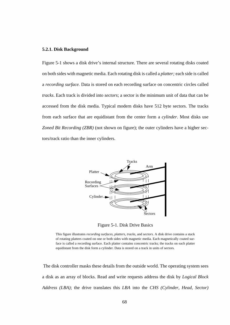
68
5.2.1. Disk Background
Figure 5-1 shows a disk drive’s internal structure. There are several rotating disks coated
on both sides with magnetic media. Each rotating disk is called a platter; each side is called
a recording surface. Data is stored on each recording surface on concentric circles called
tracks. Each track is divided into sectors; a sector is the minimum unit of data that can be
accessed from the disk media. Typical modern disks have 512 byte sectors. The tracks
from each surface that are equidistant from the center form a cylinder. Most disks use
Zoned Bit Recording (ZBR) (not shown on figure); the outer cylinders have a higher sec-
tors/track ratio than the inner cylinders.
The disk controller masks these details from the outside world. The operating system sees
a disk as an array of blocks. Read and write requests address the disk by Logical Block
Address (LBA); the drive translates this LBA into the CHS (Cylinder, Head, Sector)
Figure 5-1. Disk Drive Basics
This figure illustrates recording surfaces, platters, tracks, and sectors. A disk drive contains a stackof rotating platters coated on one or both sides with magnetic media. Each magnetically coated sur-face is called a recording surface. Each platter contains concentric tracks; the tracks on each platterequidistant from the disk form a cylinder. Data is stored on a track in units of sectors.
ArmPlatter
Cylinder
Tracks
RecordingSurfaces
Sectors

69
address. Logical block numbering starts with the outermost tracks and continues inward
with each successive cylinder. Therefore, the sector after the last of any given track is the
first of the next track in the same cylinder.
Each recording surface has its own read head and write head. The heads are ganged
together on the disk arm. The time to move the arm to the right track is called Seek Time
and the time for the required sector to rotate under the head is called Rotational Latency.
The time to transfer the data from the media is called Transfer Time. In modern disks, only
one head is active at any time. When an access spans two tracks, the disk must complete
the portion on the first track, switch heads, and continue on the second track. The sector
mappings on consecutive tracks are skewed to allow for this Head Switch time. Switching
heads requires a short repositioning time; the skew prevents a request that crosses track
boundaries from missing the next logical block and having to wait a full rotation. Similarly,
if an access spans two cylinders, the disk arm has to seek forward one cylinder. Consecu-
tive cylinders are skewed to allow for this Cylinder Switch Time.
5.2.2. Related Work
Saavedra [Saavedra92, Saavedra94] introduced a simple, yet powerful, mechanism to
extract performance characteristics from a multi-level memory hierarchy. The benchmark
repeatedly executes a loop of reading memory locations in a fixed size array at a given
stride. Surprisingly, almost all the characteristics of the memory hierarchy, including
number of caches, their capacity, associativity, block size, and access times, can be
extracted by changing the size of the array and the length of the stride. This technique,

70
unfortunately, cannot be applied directly to disk drives. The complex interaction between
mechanical and electronics functions makes the results much more unpredictable and dif-
ficult to decipher than the those that occur when the benchmark is run on a memory hier-
archy.
Ganger and Worthington [Worthington95] described partially automated tools for extract-
ing parameters from SCSI disk drives. They used a twofold approach, interrogative and
empirical extraction. Interrogative extraction uses a library of SCSI access functions to
read the disk’s Mode Pages. The mode pages describe disk parameters like the sectors/
track ratio, prefetch buffer size, and so on. The information extracted from the mode pages
is used to construct test vectors for the empirical extraction process. They measured the
minimum time between requests (MTBRC) of various kinds. By comparing the MTBRCs
of different test vectors, they calculate switching times and other parameters.
The main disadvantage of this approach is that the user needs to know about the SCSI sub-
system. In particular, the user must be able to send low level SCSI commands to the disks,
requiring in turn that each drive manufacturer support the required commands. If the disk
is not SCSI, but IDE, then the user would need access to low level IDE commands. Also,
each parameter requires a separate group of test vectors. The ideal benchmark would com-
bine the simplicity and elegance of the Saavedra solution to the accuracy of the Ganger and
Worthington approach.

71
5.3. The Write Benchmark
This section describes the write version of the Skippy benchmark. We present the algo-
rithm and use a simple analytical model to illustrate the behavior that we expect. We
parametrize this analytical model with a synthetic disk and show the expected graphical
result. Next, we present the results on an actual disk, the IBM Ultrastar XP. Finally, we
extract the IBM disk’s geometry and switching latencies from the result graph and compare
them to the manufacturer specified values.
5.3.1. The Algorithm
The benchmark does a sequence of single sector writes and seeks through the raw device
interface; Figure 5-2 shows the pseudocode. By using the raw device interface, we can
bypass file optimizations activities like caching, buffering, and read ahead. The benchmark
writes one sector to the disk, seeks and writes again. At each iteration, the seek distance (or
StepSize) increases by one.
Figure 5-2. Pseudocode for the Write Version of Skippy.
int i;open (raw disk device);for (i=0; i< Number of Measurements;i++){
Read start time lseek(raw device, i); write(1 sector)}close (raw device);
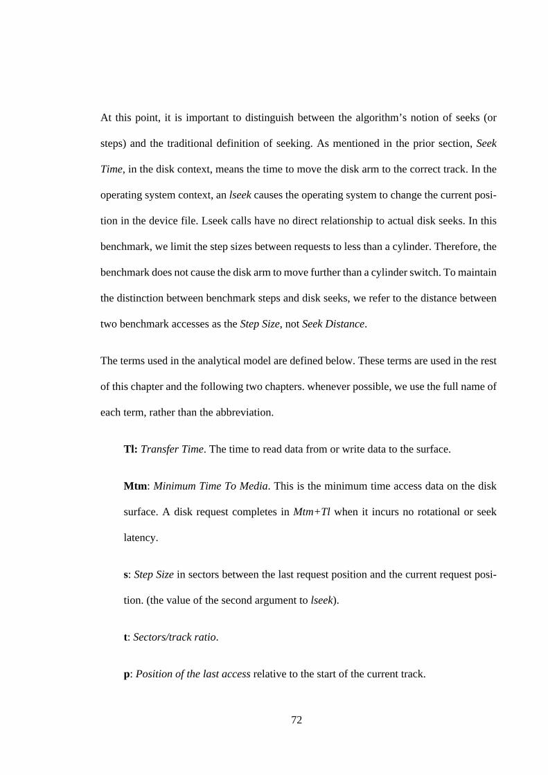
72
At this point, it is important to distinguish between the algorithm’s notion of seeks (or
steps) and the traditional definition of seeking. As mentioned in the prior section, Seek
Time, in the disk context, means the time to move the disk arm to the correct track. In the
operating system context, an lseek causes the operating system to change the current posi-
tion in the device file. Lseek calls have no direct relationship to actual disk seeks. In this
benchmark, we limit the step sizes between requests to less than a cylinder. Therefore, the
benchmark does not cause the disk arm to move further than a cylinder switch. To maintain
the distinction between benchmark steps and disk seeks, we refer to the distance between
two benchmark accesses as the Step Size, not Seek Distance.
The terms used in the analytical model are defined below. These terms are used in the rest
of this chapter and the following two chapters. whenever possible, we use the full name of
each term, rather than the abbreviation.
Tl: Transfer Time. The time to read data from or write data to the surface.
Mtm: Minimum Time To Media. This is the minimum time access data on the disk
surface. A disk request completes in Mtm+Tl when it incurs no rotational or seek
latency.
s: Step Size in sectors between the last request position and the current request posi-
tion. (the value of the second argument to lseek).
t: Sectors/track ratio.
p: Position of the last access relative to the start of the current track.

73
Rl: Time for one full rotation. We call this Full Rotation Time. Rotational Latency,
on the other hand, is the time that a given request spends waiting for the required
sector to rotate under the head. The Rotational Latency can vary anywhere between
zero and the Full Rotation Time.
Hsw: Head Switch Time.
Csw: Single Cylinder Switch Time
Stm: Number of sectors that the disk rotates in Minimum Time to Media. Equation
(1) defines Stm in terms of Mtm, t, and Rl, as
Equation 5-1.
Note that equation 5-1 assumes a linear relationship between the latency and the number
of sectors rotated. It is well known that seek time does not increase linearly with seek dis-
tance. However, as we stated earlier, the step sizes used do not generate any arm move-
ment; the delay is purely rotational. Since the disk rotates at a fixed speed, the delay
increases linearly with the number of sectors rotated.
Figure 5-3 shows the expected sequence of events for two single sector writes labeled W1
and W2. We assume that the step size between the writes is small enough that the two
requests will be on the same track. The figure shows five stages that each write goes
through; the disk rotates a few sectors between each stage. W1, starts at time W1Start. By
time W1atDisk, the OS and SCSI subsystem have processed the request and the command
has reached the disk. By time W1atSurface, the disk has positioned the head on the neces-
StmMinimumMediaTime SectorsPerTrack×
FullRotationTime-----------------------------------------------------------------------------------------------------------=
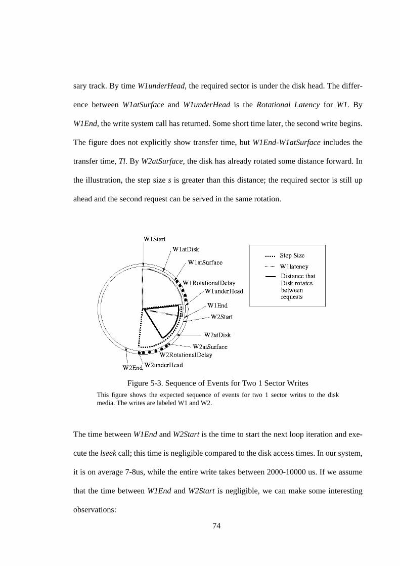
74
sary track. By time W1underHead, the required sector is under the disk head. The differ-
ence between W1atSurface and W1underHead is the Rotational Latency for W1. By
W1End, the write system call has returned. Some short time later, the second write begins.
The figure does not explicitly show transfer time, but W1End-W1atSurface includes the
transfer time, Tl. By W2atSurface, the disk has already rotated some distance forward. In
the illustration, the step size s is greater than this distance; the required sector is still up
ahead and the second request can be served in the same rotation.
The time between W1End and W2Start is the time to start the next loop iteration and exe-
cute the lseek call; this time is negligible compared to the disk access times. In our system,
it is on average 7-8us, while the entire write takes between 2000-10000 us. If we assume
that the time between W1End and W2Start is negligible, we can make some interesting
observations:
Figure 5-3. Sequence of Events for Two 1 Sector WritesThis figure shows the expected sequence of events for two 1 sector writes to the diskmedia. The writes are labeled W1 and W2.
75
(i) As the rotational delay approaches zero,W2End-W2Start becomesMinimumMedia-
Time+TransferTime.
(ii) When the rotational delay is eliminated,W2atSurface-W1atSurface is alsoMinimum-
MediaTime. Therefore, the disk rotates for approximatelyMtm time, or overStm sectors,
between any two requests. In other words, ifStepSize < Stm, W2 will need an extra rota-
tion. If StepSize>Stm, W2 can complete in the same rotation asW1.
Using the above logic, we can model the latency of the second write request. If the access
is on the same track as the prior access, (i.ep+StepSize < Sectors/Track), andStepSize >
Stm, the request can be satisfied in the current rotation and the latency is
Equation 5-2.
This latency is the minimum time to media plus the time to rotate the remaining sectors.
Substituting equation 5-1 into 5-2 gives us a simpler term for the latency:
Equation 5-3.
As the equation shows, the latency is a linear function of the step size. IfStepSize<Stm, the
request is satisfied in the next rotation, and the latency is given by equation (4):
Equation 5-4.
Equation 5-4 can also be simplified by substituting 5-1, giving equation 5-5:
LatencyStepSize Stm–( ) FullRotationTime×
SectorsPerTrack------------------------------------------------------------------------------------------------- MiminumMediaTime TransferTime+ +=
LatencyStepSize FullRotationTime×
SectorsPerTrack---------------------------------------------------------------------------- TransferTime+=
LatencySectorsPerTrack StepSize Stm–+( )
SectorsPerTrack---------------------------------------------------------------------------------------------- FullRotationTime× MinimumMediaTime TransferTime+ +=

76
Equation 5-5.
When StepSize<Stm, the latency is still linear in StepSize with the fixed vertical offset
equal to FullRotationTime. If the step puts the new request on a different track (p+StepSize
> Sectors/Track), then the request incurs an extra head switch delay. Since the tracks are
skewed, a head switch does not cause the disk to have to wait a full rotation. In this case,
the latencies can be calculated as in equations 5-6 and 5-7, When StepSize>Stm:
Equation 5-6.
When StepSize<Stm:
Equation 5-7.
The equations for a cylinder switch are similar, with CylinderSwitchTime in place of Head-
SwitchTime.
Note that all these equations assume that there are no long distance seeks going on. This
model and the benchmark are not intended to for step sizes that cause seeks greater than a
single cylinder. After that point, there is significant arm movement and the latency does
not scale linearly with step size.
LatencyStepSize FullRotationTime×
SectorsPerTrack---------------------------------------------------------------------------- FullRotationTime TransferTime+ +=
LatencyStepSize Stm–( ) FullRotationTime×
SectorsPerTrack------------------------------------------------------------------------------------------------- MinimumMediaTime HeadSwitch TransferTime+ + +=
LatencySectorsPerTrack StepSize Stm–+( )
SectorsPerTrack---------------------------------------------------------------------------------------------- Rl× MinimumMediaTime HeadSwitch TransferTime+ + +=

77
5.3.2. Graphical Result
Now we evaluate the above equations using a synthetic disk whose parameters are listed
in Table 5-1. The synthetic disk is 7200 RPM, with 15 recording surfaces containing 150
sectors per track. The minimum time to access media is 2.0 ms, and the head and cylinder
switch times are 0.7 ms and 2.1 ms respectively. Since the benchmark does not create long
distance seeks, we do not specify a seek profile.
Figure 5-4 shows the expected graphical result; the accompanying illustrations, Figures 5-
5(a-d), show what happens at points (1) through (4) in the graph. Each illustration shows
two writes; the second write shows the request pattern at the marked point in the graph.
Each track is shown as two concentric circles; the rotational delay for Write1 is marked on
the outer circle and the rotational delay for the Write2 is marked on the inner circle. The
illustrations do not show Transfer Time; since we are focusing on single sector accesses,
the transfer time is nearly negligible. We will discuss Transfer Time further when we
extract parameters in the next section and when we deal with larger transfer sizes in the
next chapter.
Parameter Value
Sectors/Track 150
Full Rotation Time 8333.33 us
Minimum Media Time 2000 us
Number of Heads 15
Head Switch Time 700.00 us
Cylinder Switch Time 2100.00 us
Table 5-1. Parameters for Synthetic Disk Drive
This table lists the parameters for a synthetic disk drive. These parameters are used in thissection and section 5.6 to illustrate the expected graphical results for the write and readversions of the benchmark.
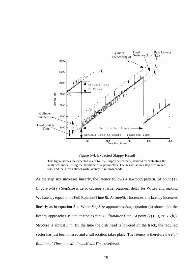
78
As the step size increases linearly, the latency follows a sawtooth pattern. At point (1),
(Figure 5-5(a)) StepSize is zero, causing a large rotational delay for Write2 and making
W2Latency equal to the Full Rotation Time Rl. As StepSize increases, the latency increases
linearly as in equation 5-4. When StepSize approaches Stm, equation (4) shows that the
latency approaches MinimumMediaTime+FullRotationTime. At point (2) (Figure 5.5(b)),
StepSize is almost Stm. By the time the disk head is lowered on the track, the required
sector has just been missed and a full rotation takes place. The latency is therefore the Full
Rotational Time plus MinimumMediaTime overhead.
Figure 5-4. Expected Skippy ResultThis figure shows the expected result for the Skippy benchmark, derived by evaluating theanalytical model using the synthetic disk parameters. The X axis shows step size in sec-tors, and the Y axis shows write latency in microseconds.
(1)
(2)
(3)
(4)
Minimum Time
To Media
Minimum Time to Media + Transfer Time
Sectors Per Track
CylinderSwitch Time
Head SwitchTime
CylinderSwitches (L4)
HeadSwitches (L3)
Base Latency(L2)
(L1)
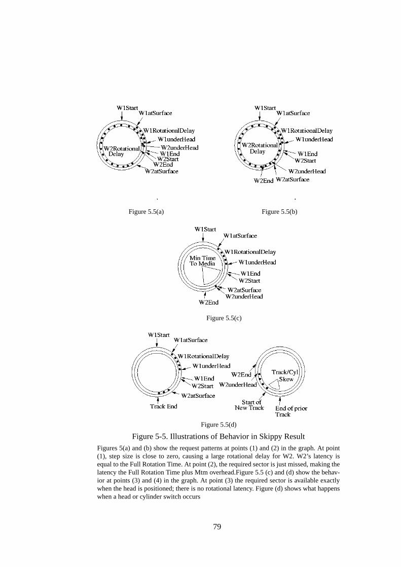
79
Figure 5-5. Illustrations of Behavior in Skippy ResultFigures 5(a) and (b) show the request patterns at points (1) and (2) in the graph. At point(1), step size is close to zero, causing a large rotational delay for W2. W2’s latency isequal to the Full Rotation Time. At point (2), the required sector is just missed, making thelatency the Full Rotation Time plus Mtm overhead.Figure 5.5 (c) and (d) show the behav-ior at points (3) and (4) in the graph. At point (3) the required sector is available exactlywhen the head is positioned; there is no rotational latency. Figure (d) shows what happenswhen a head or cylinder switch occurs
Figure 5.5(a) Figure 5.5(b)
Figure 5.5(c)
Figure 5.5(d)

80
A few steps later, we reach point (3) (Figure 5-5(c)), where StepSize is slightly larger than
Stm. In this case, the disk head is lowered just in time and there is no rotational latency.
The latency therefore becomes MinimumMediaTime. From then on, as StepSize increases,
the latency increases linearly as in equation 5-2. The graph has a sawtooth shape; the tran-
sition happens at StepSize=Stm.
The graph also shows a series of upward spikes that correspond to head and cylinder
switches. Point (4) (Figure (5-5(d)) illustrates a head switch. In this case, the rotational
latency is increased by HeadSwitchTime as specified by equation 5-6. The smaller spikes
correspond to head switches and the larger spikes correspond to cylinder switches.
5.3.3. Extracting Parameters
Figure 5-4 exposes many useful disk details. The X coordinate of point (3) is Stm and the
Y coordinate is MinimumMediaTime+TransferTime. Since the transfer time is very small
for a single sector, the Y coordinate of point (3) is a good estimate for MinimumMedia-
Time. Mtm is also the difference between the Y coordinates of points (1) and (2). FullRo-
tationTime Rl is the latency at step size 0 and the height of the transition at the
MinimumMediaTime point.
Using this information, we can calculate the number of sectors per track. Since we know
that the MinimumMediaTime point is reached when StepSize=Stm, we can reverse equation
5-1 to calculate the Sectors/Track ratio t:
Equation 5-8. SectorsPerTrackStm FullRotationTime×
MinimumMediaTime----------------------------------------------------------------=
81
Note that we can only calculate the sectors/track ratio for the region that was written. Most
modern disks employ Zone Bit Recording; outer cylinders have more sectors per track than
inner cylinders. To get the Sectors/Track ratio of other regions in the disk, we will need to
run the benchmark on those regions as well.
As StepSize increases, the latencies form three distinct lines with the same slope and dif-
ferent offsets. Figure 5-4 shows four lines labeled L1 through L4. L1 conforms to equation
5-4 and L2 conforms to equation 5-2. By taking the difference in offsets between these two
lines, we can calculate the rotation time. The slope of each line is FullRotationTime/Sec-
torsPerTrack. Once FullRotationTime is known, we can extract the Sectors/Track ratio
from the slope value.
Each point on L3 represents a head switch and the latencies conform to equation 5-6.
Hence, the vertical offset between the L3 and the L2 is HeadSwitchTime. Each point on L4
corresponds to a cylinder switch; the vertical offset between the third line and L2 is Cylin-
derSwitchTime.
Finally, while the step size is less than the number of sectors per track, we can get the
number of recording surfaces by counting the number of head switches between two cyl-
inder switches. We can also calculate the number of recording surfaces from the total step
distance between two cylinder switches. Since the benchmark moves forward with each
step, the distance between the sectors accessed at step sizes s1 and s2 is not simply s2-s1.
If we assume that the benchmark started by writing sector 0, the address of the sector writ-
ten at step size s1 is the sum of s1 iterations of the arithmetic progression starting at 0 with
increment 1. This sum is

82
Equation 5-9.
We can calculate the address of the sector written at step s2 in the same way. Taking the
difference between these two addresses gives us the actual step distance between the mea-
surements at step sizes s1 and s2. The total distance between the two accesses is
Equation 5-10.
Since we already know the number of sectors per track, the number of recording surfaces is
Equation 5-11.
As the step size gets larger, the number of steps between successive head and cylinder
switches decreases. As figure 5-4 shows, after StepSize is greater than SectorsPer-
Track+Stm, every step causes a head switch.
5.3.4. A Sample Result
The prior section showed how all the parameters in Table 5-1 can be extracted from Figure
5.4. Now we apply these techniques to the IBM UltraStar XP disk drive [UltraStar96].
From the manufacturer specifications we learn that this disk is 7200 RPM (8.33 ms rota-
tional latency), with 9 platters (18 recording surfaces) and 8 recording zones, the outermost
of which has 184 sectors per track. The head and cylinder switch times are 0.85 ms and
2.17 ms respectively.
s1 s1 1+( )×2
-------------------------------
StepDists2 s1–( )
2---------------------- 2s1 s2 s1–( )+( )×=
RecordingSurfaces StepDistSectorsPerTrack---------------------------------------------=
83
Figure 5-6 shows the result of running the benchmark on this disk; the figure is quite sim-
ilar to the model result in Figure 5-4. The result follows the behavior predicted by equa-
tions 5-1 through 5-6. Equation 5-7, however, does not completely explain the result of
head and cylinder switches while StepSize<Stm. In Figure 5-4, head switches always cause
upward latency spikes consistent with 5-7; figure 5-6 shows upward spikes for small Step-
Size and also some downward spikes as StepSize approaches Stm. This variation does not
affect our ability to extract the necessary parameters, but it does require a refinement of the
analytical model. We refine the model in Section 5-4; for now, we focus on extracting
parameters from Figure 5-6.
Following the parameter extraction techniques described earlier, we get the following mea-
sured values. FullRotationTime from the Y coordinate at point (1) is 8.39ms; the actual
latency is 8.33ms and the error is 0.73%. If we use the height of the sawtooth wave to esti-
mate Rl, we get 8.30ms. In this case, the error is 0.43%. Both techniques for estimating Rl
yield extremely accurate results.
The X coordinate value of point (3) is 47 and the Y coordinate value is 2.20ms. As equation
(2) states, the offset of L2 is the Transfer Time; this value is 0.06ms. Since we are writing
only 512 bytes, the transfer time is very small. By subtracting Transfer Time from the Y
coordinate value at point 3, we estimate MinimumMediaTime to be 2.1 ms. In fact, since
the transfer time is so small, its effect on the Mtm value is virtually indistinguishable from
measurement noise and the Y coordinate value is itself a good estimate of Mtm. On the
other hand, if we estimate Mtm as the difference between the Y values at points (1) and
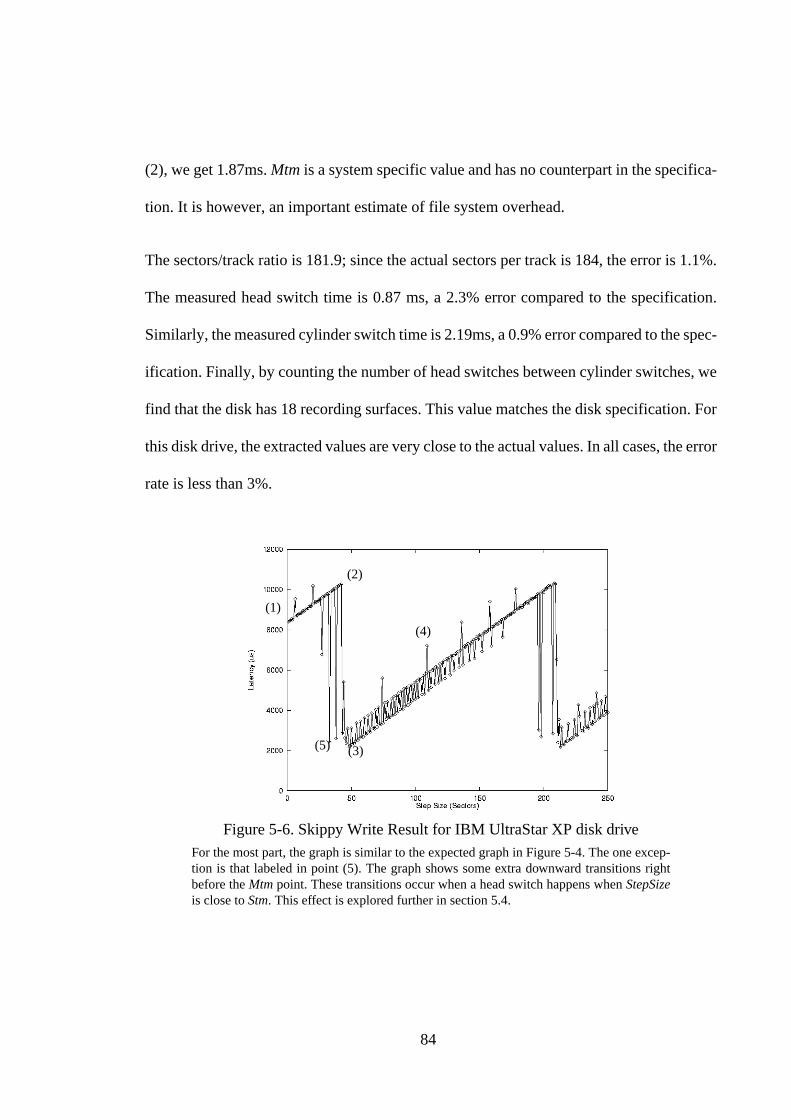
84
(2), we get 1.87ms. Mtm is a system specific value and has no counterpart in the specifica-
tion. It is however, an important estimate of file system overhead.
The sectors/track ratio is 181.9; since the actual sectors per track is 184, the error is 1.1%.
The measured head switch time is 0.87 ms, a 2.3% error compared to the specification.
Similarly, the measured cylinder switch time is 2.19ms, a 0.9% error compared to the spec-
ification. Finally, by counting the number of head switches between cylinder switches, we
find that the disk has 18 recording surfaces. This value matches the disk specification. For
this disk drive, the extracted values are very close to the actual values. In all cases, the error
rate is less than 3%.
Figure 5-6. Skippy Write Result for IBM UltraStar XP disk driveFor the most part, the graph is similar to the expected graph in Figure 5-4. The one excep-tion is that labeled in point (5). The graph shows some extra downward transitions rightbefore the Mtm point. These transitions occur when a head switch happens when StepSizeis close to Stm. This effect is explored further in section 5.4.
(1)
(2)
(3)
(4)
(5)

85
5.4. A Refined Analytical Model For Writes
Figure 5-6 showed that the simple model is inadequate for describing some parts of the
benchmark behavior. In particular, the graph shows some downward spikes in the region
StepSize<Stm that are not explained by equation 5-7. In this section, we present a refine-
ment to the initial model to explain these effects.
In Figure 5-6, the downward spikes near point (5) happen when a head switch occurs while
StepSize is close to Stm. In normal circumstances, when there is no head switch, the
mechanics of equation 5-4 apply; there is not enough time to position the head and service
the write in the same rotation as the prior write. When a head switch occurs, however, the
track skew gives the disk head slightly extra time, enabling the disk to service some writes
without waiting an extra rotation. These writes can complete with latencies close to Mtm.
Figure 5-6 shows that these downward spikes actually extend L3, the head switch line, to
the left of the Mtm point. This observation confirms our hypothesis that the spikes are
caused by head switches.
To refine the model, we need to break Mtm down into two parts:
Mov: The sum of operating system, SCSI and disk electronics overheads to process
the request.
Sov: The number of sectors the disk rotates in time Mov.
Mdp : The disk positioning time. This is the minimum time needed for the disk to
position the arm over the required track.

86
Mov is the minimum time between the disk’s completing the first request and receiving the
second request. Any request where StepSize<Sov is not serviceable within the current rota-
tion whether it includes a head switch or not. The gray area is when Sov <StepSize < Stm.
Equation 5-12 gives the write latency when Sov< Size < Stm, p+StepSize > Sectorsper-
Track and a head switch occurs:
Equation 5-12.
Once again, the latency when a cylinder switch occurs can be calculated by replacing
HeadSwitchTime in equation 5-8 with CylinderSwitchTime.
To evaluate the refined model, we need to add two parameters for the synthetic disk’s pro-
file in Table 5-1 We assume that Mov and Mdp are each 1.0 ms. Figure 5-7 shows the
refined model parametrized for the synthetic disk.; the refined model shows the downward
spikes as expected. We can use the step size at which the first downward spike occurred to
estimate the value of Mdp, and hence Mov. Therefore, we can get finer estimates of oper-
ating system/interconnect overheads as well as estimates of disk positioning time.
In Figure 5-6, the result for the IBM disk, the first downward spike happened at step size
33. The Mtm point was at step 47. Therefore, we can estimate Mdp as the time taken to
rotate 47-33, or 14 sectors. This time is 634 us. Since Mdp and Mov add to Mtm, Mov is
1565 us.
LatencyStepSize Sov–( ) FullRotationTime×
SectorsPerTrack------------------------------------------------------------------------------------------------- Mov HeadSwitchTime TransferTime+ + +=
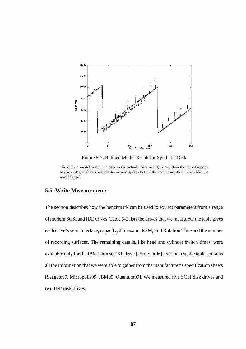
87
5.5. Write Measurements
The section describes how the benchmark can be used to extract parameters from a range
of modern SCSI and IDE drives. Table 5-2 lists the drives that we measured; the table gives
each drive’s year, interface, capacity, dimension, RPM, Full Rotation Time and the number
of recording surfaces. The remaining details, like head and cylinder switch times, were
available only for the IBM UltraStar XP drive [UltraStar96]. For the rest, the table contains
all the information that we were able to gather from the manufacturer’s specification sheets
[Seagate99, Micropolis99, IBM99, Quantum99]. We measured five SCSI disk drives and
two IDE disk drives.
Figure 5-7. Refined Model Result for Synthetic Disk
The refined model is much closer to the actual result in Figure 5-6 than the initial model.In particular, it shows several downward spikes before the main transition, much like thesample result.
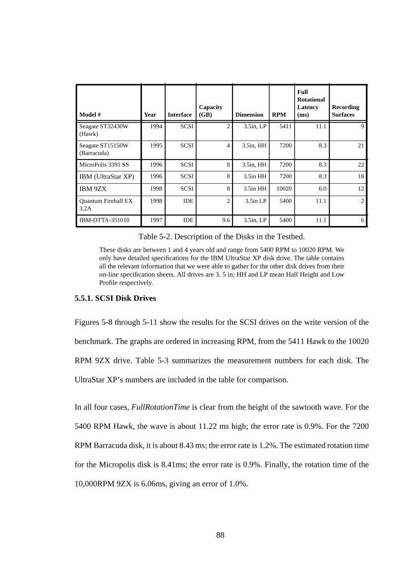
88
5.5.1. SCSI Disk Drives
Figures 5-8 through 5-11 show the results for the SCSI drives on the write version of the
benchmark. The graphs are ordered in increasing RPM, from the 5411 Hawk to the 10020
RPM 9ZX drive. Table 5-3 summarizes the measurement numbers for each disk. The
UltraStar XP’s numbers are included in the table for comparison.
In all four cases, FullRotationTime is clear from the height of the sawtooth wave. For the
5400 RPM Hawk, the wave is about 11.22 ms high; the error rate is 0.9%. For the 7200
RPM Barracuda disk, it is about 8.43 ms; the error rate is 1.2%. The estimated rotation time
for the Micropolis disk is 8.41ms; the error rate is 0.9%. Finally, the rotation time of the
10,000RPM 9ZX is 6.06ms, giving an error of 1.0%.
Model # Year InterfaceCapacity(GB) Dimension RPM
FullRotationalLatency(ms)
RecordingSurfaces
Seagate ST32430W(Hawk)
1994 SCSI 2 3.5in, LP 5411 11.1 9
Seagate ST15150W(Barracuda)
1995 SCSI 4 3.5in, HH 7200 8.3 21
MicroPolis 3391 SS 1996 SCSI 8 3.5in, HH 7200 8.3 22
IBM (UltraStar XP) 1996 SCSI 8 3.5in HH 7200 8.3 18
IBM 9ZX 1998 SCSI 8 3.5in HH 10020 6.0 12
Quantum Fireball EX3.2A
1998 IDE 2 3.5in LP 5400 11.1 2
IBM-DTTA-351010 1997 IDE 9.6 3.5in, LP 5400 11.1 6
Table 5-2. Description of the Disks in the Testbed.
These disks are between 1 and 4 years old and range from 5400 RPM to 10020 RPM. Weonly have detailed specifications for the IBM UltraStar XP disk drive. The table containsall the relevant information that we were able to gather for the other disk drives from theiron-line specification sheets. All drives are 3. 5 in; HH and LP mean Half Height and LowProfile respectively.
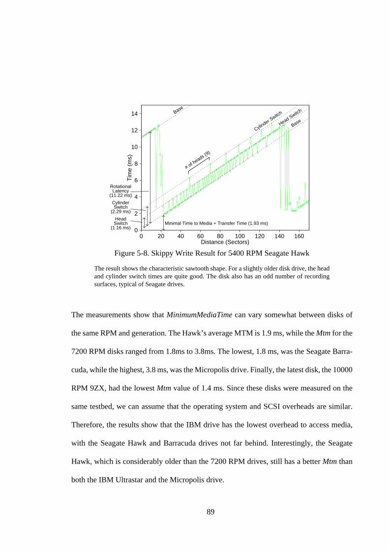
89
The measurements show that MinimumMediaTime can vary somewhat between disks of
the same RPM and generation. The Hawk’s average MTM is 1.9 ms, while the Mtm for the
7200 RPM disks ranged from 1.8ms to 3.8ms. The lowest, 1.8 ms, was the Seagate Barra-
cuda, while the highest, 3.8 ms, was the Micropolis drive. Finally, the latest disk, the 10000
RPM 9ZX, had the lowest Mtm value of 1.4 ms. Since these disks were measured on the
same testbed, we can assume that the operating system and SCSI overheads are similar.
Therefore, the results show that the IBM drive has the lowest overhead to access media,
with the Seagate Hawk and Barracuda drives not far behind. Interestingly, the Seagate
Hawk, which is considerably older than the 7200 RPM drives, still has a better Mtm than
both the IBM Ultrastar and the Micropolis drive.
Figure 5-8. Skippy Write Result for 5400 RPM Seagate Hawk
The result shows the characteristic sawtooth shape. For a slightly older disk drive, the headand cylinder switch times are quite good. The disk also has an odd number of recordingsurfaces, typical of Seagate drives.
0
2
4
6
8
10
12
14
0 20 40 60 80 100 120 140 160
Tim
e (m
s)
Distance (Sectors)
Base
Cylinder S
witch
Head Switch
Base
# of heads (
9)
Minimal Time to Media + Transfer Time (1.93 ms)
RotationalLatency
(11.22 ms)
CylinderSwitch
(2.29 ms)
HeadSwitch
(1.16 ms)

90
Since all of the measured drives employ Zone Bit Recording, we extract the Sectors/Track
ratio for the outermost zone of each drive. The Hawk has around 142 sectors per track, the
Barracuda about 123, the UltraStar 186, the Micropolis 201, and the 9ZX about 224.
Finally, we compare the head and cylinder switch times. As the graphs show, the Seagate
Barracuda drive has the lowest head and cylinder switch times. The Hawk’s cylinder
switch time is comparable to that of the UltraStar XP, even though the Hawk is an older
drive.
By counting the number of head switches between cylinder, we learn that the Hawk has 9
recording surfaces, the Barracuda has 21, the Micropolis has 22, and the 9ZX has 12. The
numbers for the Hawk, Barracuda and 9ZX match the specification data in Table 5-2.
Figure 5-9. Skippy Write Result for 7200 RPM Seagate Barracuda
Like the previous figure, the Barracuda result shows very good switching times and an oddnumber of recording surfaces, typical of Seagate disk drives.
0
2
4
6
8
10
12
0 20 40 60 80 100 120 140 160
Tim
e (m
s)
Distance (Sectors)
Base
Cylinder Switch
Head Switch
Base
# of heads (2
1)
Minimal Time to Media + Transfer Time (2.01 ms)
RotationalLatency
(8.43 ms)
CylinderSwitch
(1.32 ms)
HeadSwitch
(0.76 ms)
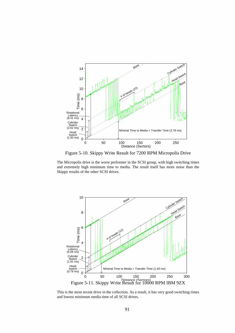
91
Figure 5-10. Skippy Write Result for 7200 RPM Micropolis Drive
The Micropolis drive is the worst performer in the SCSI group, with high switching timesand extremely high minimum time to media. The result itself has more noise than theSkippy results of the other SCSI drives.
Figure 5-11. Skippy Write Result for 10000 RPM IBM 9ZX
This is the most recent drive in the collection. As a result, it has very good switching timesand lowest minimum media time of all SCSI drives.
0
2
4
6
8
10
12
14
0 50 100 150 200 250
Tim
e (m
s)
Distance (Sectors)
Base
Cylinder Switch
Head Switch
Base
# of heads (22)
Minimal Time to Media + Transfer Time (3.78 ms)
RotationalLatency
(8.41 ms)
CylinderSwitch
(2.62 ms)
HeadSwitch
(1.50 ms)
0
2
4
6
8
10
0 50 100 150 200 250 300
Tim
e (m
s)
Distance (Sectors)
Base
BaseHead SwitchCylinder S
witch
# of heads (12)
Minimal Time to Media + Transfer Time (1.40 ms)
RotationalLatency
(6.06 ms)
CylinderSwitch
(1.91 ms)
HeadSwitch
(0.79 ms)
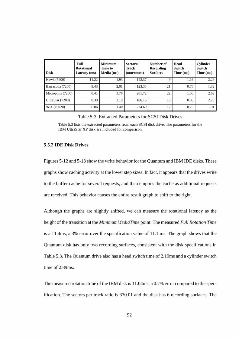
92
5.5.2 IDE Disk Drives
Figures 5-12 and 5-13 show the write behavior for the Quantum and IBM IDE disks. These
graphs show caching activity at the lower step sizes. In fact, it appears that the drives write
to the buffer cache for several requests, and then empties the cache as additional requests
are received. This behavior causes the entire result graph to shift to the right.
Although the graphs are slightly shifted, we can measure the rotational latency as the
height of the transition at the MinimumMediaTime point. The measured Full Rotation Time
is a 11.4ms, a 3% error over the specification value of 11.1 ms. The graph shows that the
Quantum disk has only two recording surfaces, consistent with the disk specifications in
Table 5.3. The Quantum drive also has a head switch time of 2.19ms and a cylinder switch
time of 2.89ms.
The measured rotation time of the IBM disk is 11.04ms, a 0.7% error compared to the spec-
ification. The sectors per track ratio is 330.01 and the disk has 6 recording surfaces. The
Disk
FullRotationalLatency (ms)
MinimumTime toMedia (ms)
Sectors/Track(outermost)
Number ofRecordingSurfaces
HeadSwitchTime (ms)
CylinderSwitchTime (ms)
Hawk (5400) 11.22 1.93 142.37 9 1.16 2.29
Barracuda (7200) 8.43 2.01 123.35 21 0.76 1.32
Micropolis (7200) 8.41 3.78 201.72 22 1.50 2.62
UltraStar (7200) 8.39 2.19 186.15 18 0.85 2.20
9ZX (10020) 6.06 1.40 224.69 12 0.79 1.91
Table 5-3. Extracted Parameters for SCSI Disk Drives
Table 5.3 lists the extracted parameters from each SCSI disk drive. The parameters for theIBM UltraStar XP disk are included for comparison.
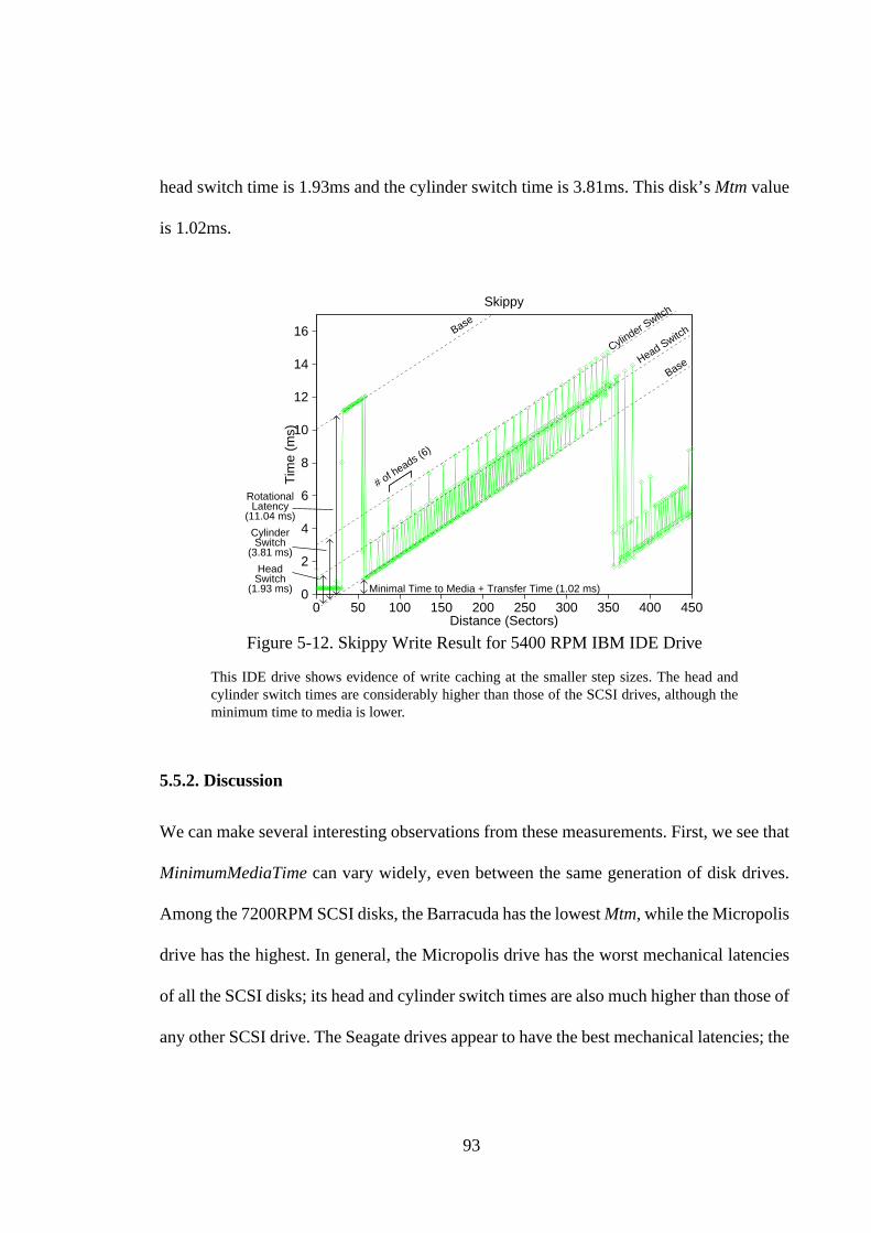
93
head switch time is 1.93ms and the cylinder switch time is 3.81ms. This disk’s Mtm value
is 1.02ms.
5.5.2. Discussion
We can make several interesting observations from these measurements. First, we see that
MinimumMediaTime can vary widely, even between the same generation of disk drives.
Among the 7200RPM SCSI disks, the Barracuda has the lowest Mtm, while the Micropolis
drive has the highest. In general, the Micropolis drive has the worst mechanical latencies
of all the SCSI disks; its head and cylinder switch times are also much higher than those of
any other SCSI drive. The Seagate drives appear to have the best mechanical latencies; the
Figure 5-12. Skippy Write Result for 5400 RPM IBM IDE Drive
This IDE drive shows evidence of write caching at the smaller step sizes. The head andcylinder switch times are considerably higher than those of the SCSI drives, although theminimum time to media is lower.
0
2
4
6
8
10
12
14
16
0 50 100 150 200 250 300 350 400 450
Tim
e (m
s)
Distance (Sectors)
Skippy
Base
Cylinder Switch
Head Switch
Base
# of heads (6
)
Minimal Time to Media + Transfer Time (1.02 ms)
RotationalLatency
(11.04 ms)
CylinderSwitch
(3.81 ms)
HeadSwitch
(1.93 ms)
94
Barracuda’s switching times are lower than the 9ZX, even though the 9ZX is a newer disk.
Even the 5400 Hawk’s switching times are comparable with the 7200RPM drives.
Second, the number of recording surfaces varies widely between disks. In general, the
number of recording surfaces increases with capacity and decreases over time. For
instance, the IBM 9ZX has the same capacity as the Barracuda and UltraStar, but has less
recording surfaces because it is a newer disk, most likely with a higher areal density. The
results also show that some disks have an odd number of recording surfaces. When we first
took these measurements, we were surprised to find an odd number of heads, since it
implies that one side of one of the platters is not used.
Figure 5-13. Skippy Write Result for 5400 RPM Quantum Fireball IDE Drive
Like the previous IDE drive, this result also shows evidence of write caching, higherswitch times, and lower minimum time to media.
0
2
4
6
8
10
12
14
0 50 100 150 200 250 300 350 400
Tim
e (m
s)
Distance (Sectors)
Skippy
Base
Cylinder Switch
Head Switch
Base
# of heads (2
)
Minimal Time to Media + Transfer Time (1.25 ms)
RotationalLatency
(11.40 ms)
CylinderSwitch
(2.89 ms)
HeadSwitch
(2.19 ms)
95
Finally, if we compare the SCSI and IDE disk results, we see that the IDE disks have a
much lower MinimumMediaTime than the SCSI disks. Both IDE disks also show buffering
activity at the smaller step sizes, something we did not see with any of the SCSI disks. The
switching times of the IDE disks are also considerably higher than the SCSI disks.
5.6. Read Benchmark
The prior sections explored the benchmark’s behavior when the accesses are single sector
writes. Now we look at what happens if reads are used instead. The main advantage of
using reads is that the benchmark can be run on a disk without damaging its contents. How-
ever, reads are more complicated than writes because many disks employ read ahead opti-
mizations. The disk maintains a prefetch buffer; after the current sector is read, the disk
reads the next few sectors into this buffer. If the request pattern is sequential, the next
desired sector could be in the prefetch buffer before the request arrives. Each disk manu-
facturer has its own algorithm for read ahead. As we will see in the next few sections, such
optimizations can make read results widely different between disks of different manufac-
turers.
In this section, we explore the read behavior by creating an analytical model and parame-
terizing it with our synthetic disk. This way, we illustrate how the graphs will look under
different read ahead policies. We also describe how to extract parameters from read graphs.
We round out this section by presenting the result for the IBM UltraStar XP disk.

96
5.6.1. Expected Behavior
We begin, as we did in section 5.3.1, by outlining the expected result of the benchmark.
Unlike the write experiment, where all requests are handled in the same way by the disk,
each request in the read benchmark falls into one of three distinct categories. A request’s
category defines what the disk needs to do to service the request and hence determines the
request latency. The three categories are:
(i) In Prefetch Buffer: In the time between when the prior request completed and the cur-
rent request arrived at the disk, the sector had been read into the prefetch buffer. In this
case, the disk’s task is very simple, return the sector from the prefetch buffer.
(ii) Immediately Ahead In Read Path: The required sector is not in the prefetch buffer but
is immediately ahead in the read path. The disk chooses to read all sectors between the cur-
rent sector and the requested sector. Hence, the disk does not have to reposition the head,
merely wait till the required sector rotates under the head.
(iii) Far From Read Path: In this case, the required sector is far away from the sector cur-
rently being read. The disk will stop the ongoing read process and reposition the head to
serve the new request.
Each disk’s will have a different read ahead algorithm. Therefore, the transitions between
the above three categories will occur at different step sizes in different disks. Where the
transitions occur determines the shape of the result curve. We use the following terms to
define the transition points in our initial model:

97
Mbuffer: Minimum time to read a sector’s worth of data that is in the read-ahead
buffer.
Sbuffer: Number of sectors read into the disk buffer in time Mbuffer. This is also
the number of sectors that the disk rotates in time Mbuffer.
Sreposition: The value of StepSize at which the transition between categories (ii)
and (iii) occurs.
For small values of StepSize, the required sector will already be in the prefetch buffer when
the request arrives. The latency for category (i) requests is Mbuffer. Since the disk can read
Sbuffer sectors between successive category (i) requests, the number of sectors in the
prefetch buffer increases by Sbuffer at each step. In other words, by step s, there are
SBuffer*s sectors in the prefetch buffer. The transition between categories (i) and (ii)
occurs when the required sector is not in the prefetch buffer. For the moment, we assume
that any sector read into the prefetch buffer us not replaced by incoming sectors before it
is read. Using equation 5-9 to specify the address read at step s, we can calculate that the
transition will happen when
Equation 5-13.
In other words, when the sector to be read is ahead at step s is ahead of all sectors read by
step StepSize.
While the request is in category (ii), the disk will chose to not to reposition the head and
will wait for the required sector to rotate under the head. Therefore the latency for requests
StepSize StepSize 1+( )×2
----------------------------------------------------------------- Sbuffer StepSize×≥

98
in category (ii) is given by the minimum overhead to access a sector without positioning
the head, plus whatever rotational delay is incurred by each request. This latency is given
by:
Equation 5-14.
Note that in this case, the time between successive requests is Mov, during which the disk
rotates Sov sectors.
The transition between categories (ii) and (iii) occurs when the required sector is far
enough away that disk chooses not to read all the sectors in between. Hence, the disk repo-
sitions the head near the requested sector. In different disks, this transition will take place
at different values of StepSize. The transition point could be related to the size of the
prefetch buffer in some disks. We define the step size where the transition occurs as Srepo-
sition. After this point, the read requests behave in much the same way as the write
requests. If StepSize>Stm, where Stm is the number of sectors that the disk rotates in Min-
imumMediaTime, then the request will complete in the same rotation. If StepSize<Stm,
then the request will need one extra rotation. As before, if there is a head or cylinder switch
in either a category (ii) or category (iii) request, the head/cylinder switch time is added to
the read latency.
We can now use this model to explore the types of result curves we are likely to see in var-
ious conditions. We use the synthetic model profile from Sections 5.3 and 5.4. We also
assume that Mbuffer is 0.5 ms. Figure 5-14 shows the graphical result for Sreposition=30.
The accompanying illustrations in Figures 5-15 (a-c) explain the behavior at points (1)
LatencyStepSize Sov–( ) FullRotationTime×
SectorsPerTrack------------------------------------------------------------------------------------------------- Mov TranferTime+ +=
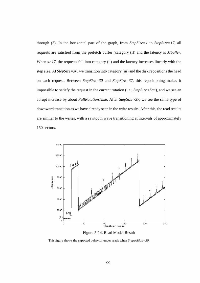
99
through (3). In the horizontal part of the graph, from StepSize=1 to StepSize=17, all
requests are satisfied from the prefetch buffer (category (i)) and the latency is Mbuffer.
When s>17, the requests fall into category (ii) and the latency increases linearly with the
step size. At StepSize=30, we transition into category (iii) and the disk repositions the head
on each request. Between StepSize=30 and StepSize=37, this repositioning makes it
impossible to satisfy the request in the current rotation (i.e., StepSize<Stm), and we see an
abrupt increase by about FullRotationTime. After StepSize>37, we see the same type of
downward transition as we have already seen in the write results. After this, the read results
are similar to the writes, with a sawtooth wave transitioning at intervals of approximately
150 sectors.
Figure 5-14. Read Model Result
This figure shows the expected behavior under reads when Sreposition=30.
(1)(2)
(3)

100
Since the read behavior is considerably more complex than the write behavior, this model
is particularly useful to show how the shape of the curve is likely to change with small dif-
ferences in the read ahead policy. Figures 5-16 (a) and (b) show the expected behavior for
Sreposition values 100 and 1000. In Figure 5-16 (a), by the time the disk decides to repo-
sition the head on each request, StepSize is already greater than Stm and none of the
requests incur an extra rotation. Therefore, the latency increases linearly with s the initial
downward transition takes place.
Figure 5-15. Illustrations of Request BehaviorFigure 5-15 (a) and (b) show the request behavior at points (1) and (2) in Figure 5.10.
Figure 5-15(a) Figure 5-15(b)
Figure 5-15(c)
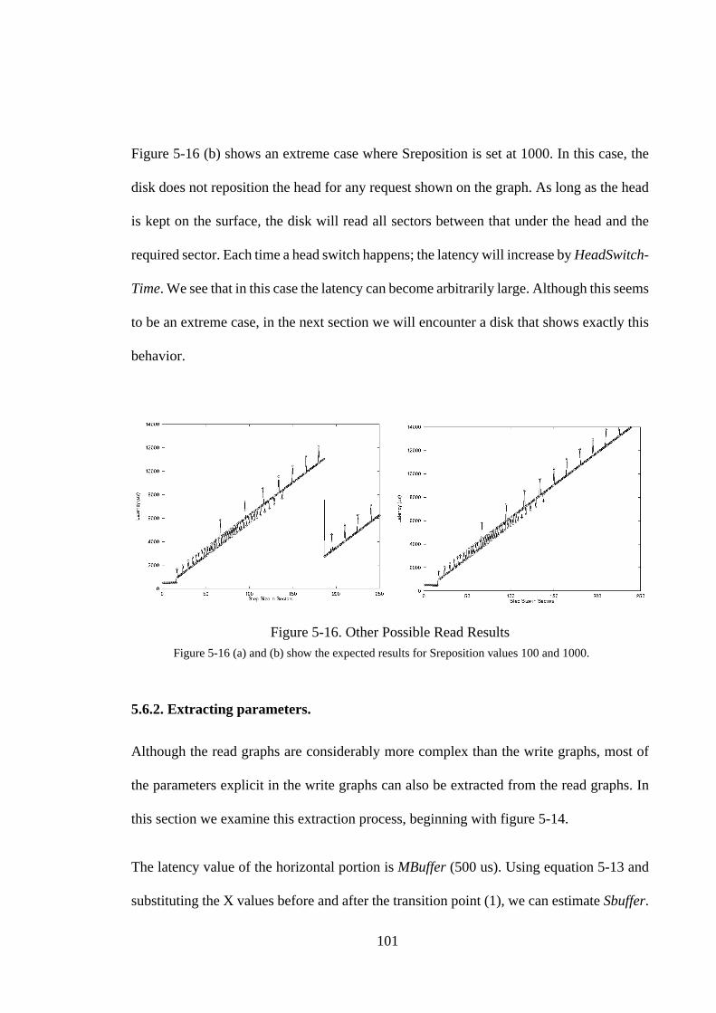
101
Figure 5-16 (b) shows an extreme case where Sreposition is set at 1000. In this case, the
disk does not reposition the head for any request shown on the graph. As long as the head
is kept on the surface, the disk will read all sectors between that under the head and the
required sector. Each time a head switch happens; the latency will increase by HeadSwitch-
Time. We see that in this case the latency can become arbitrarily large. Although this seems
to be an extreme case, in the next section we will encounter a disk that shows exactly this
behavior.
5.6.2. Extracting parameters.
Although the read graphs are considerably more complex than the write graphs, most of
the parameters explicit in the write graphs can also be extracted from the read graphs. In
this section we examine this extraction process, beginning with figure 5-14.
The latency value of the horizontal portion is MBuffer (500 us). Using equation 5-13 and
substituting the X values before and after the transition point (1), we can estimate Sbuffer.
Figure 5-16. Other Possible Read ResultsFigure 5-16 (a) and (b) show the expected results for Sreposition values 100 and 1000.

102
The height of the sawtooth wave is FullRotationTime. As in the write case, we can use the
slopes of the lines to find Sectors/Track. The head switch time, cylinder switch time, and
number of heads, are all determined in the same way as in the write graphs.
The main difference between graphs 5-14 and 5-15 (a) is that MinimumMediaTime is not
obvious in the early part of figure 5-15 (a). We can, however, determine both Mtm and
FullRotationTime from the sawtooth transition near StepSize=175. The height of the tran-
sition is still Rl; if a head switch has occurred, the Y coordinate at the bottom of the tran-
sition could be MinimumMediaTime+HeadSwitchTime+TransferTime. Since
HeadSwtchTime is known, we can estimate MinimumMediaTume as before. We can also
get MinimumMediaTime by subtracting FullRotationTime from the highest Y value in the
wave.
Finally, in the third graph, Figure 5-16(b), we have lost all the information embedded in
the transitions. We can still determine Mbuffer, HeadSwitchTime, CylinderSwitchTime and
the number of heads. However, without knowing FullRotationTime, we cannot find Sec-
tors/Track.
5.6.3. A Sample Result
Figure 5-17 shows the UltraStar XP’s result on the read benchmark. This result is similar
to Figure 5-14. Using the techniques outlined in the last section, we can extract the follow-
ing parameters:
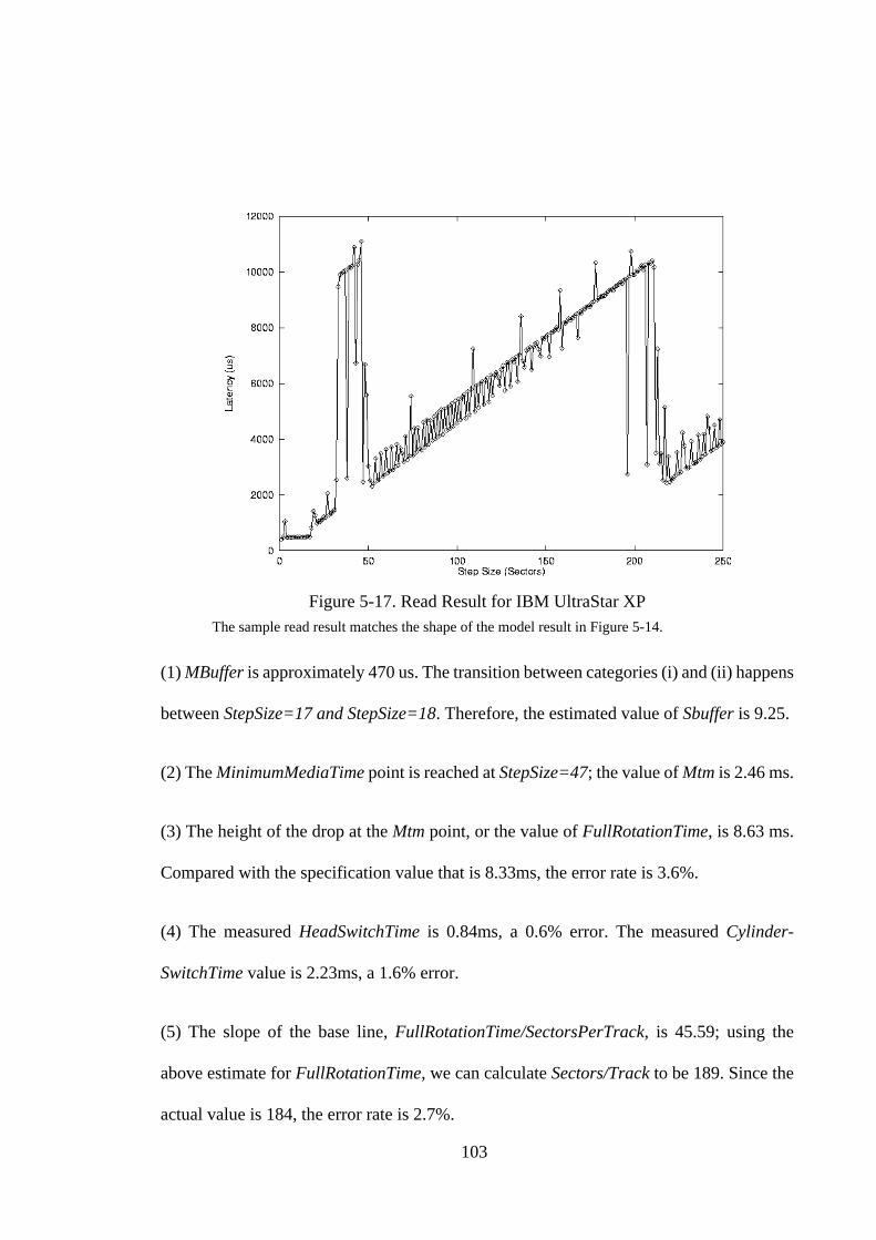
103
(1) MBuffer is approximately 470 us. The transition between categories (i) and (ii) happens
between StepSize=17 and StepSize=18. Therefore, the estimated value of Sbuffer is 9.25.
(2) The MinimumMediaTime point is reached at StepSize=47; the value of Mtm is 2.46 ms.
(3) The height of the drop at the Mtm point, or the value of FullRotationTime, is 8.63 ms.
Compared with the specification value that is 8.33ms, the error rate is 3.6%.
(4) The measured HeadSwitchTime is 0.84ms, a 0.6% error. The measured Cylinder-
SwitchTime value is 2.23ms, a 1.6% error.
(5) The slope of the base line, FullRotationTime/SectorsPerTrack, is 45.59; using the
above estimate for FullRotationTime, we can calculate Sectors/Track to be 189. Since the
actual value is 184, the error rate is 2.7%.
Figure 5-17. Read Result for IBM UltraStar XPThe sample read result matches the shape of the model result in Figure 5-14.

104
(6) Finally, counting the number of head switches between cylinder switches gives us 18,
the correct number of recording surfaces.
The parameters extracted from the read graph are also very accurate; the maximum error
rate is 3.6%. As expected, we see that there is a slight difference between the read Mini-
mumMediaTime value and the write MinimumMediaTime value.
5.7. Read Measurements
Now we examine the read results for the remaining disks in Table 5-2. Figures 5-18(a-d)
show the read results for the SCSI disks and figures 5-19(a and b) show the results for the
IDE disks. Figure 5-20 shows that each disk behaves quite differently. The X and Y scales
are the same for all graphs except 5-18(b), the Seagate Barracuda drive.
5.7.1. SCSI Disk Drives
Table 5-4 contains the parameters extracted from Figures 5-18(a-d). The UltraStar XP’s
parameters are also included for comparison. We begin with the Seagate Hawk. This drive
has the expected sawtooth behavior, the curve differs from its write counterpart at the
smaller step sizes where the read ahead activity comes into play. The Hawk’s read behavior
differs from the UltraStar XP in one important respect; Figure 5-18(a) does not show the
latency increase similar to that in point (3) of Figure 5-17. In the Hawk’s case, the transi-
tion between categories (i) and (ii) happens well past the MinimumMediaTime point, and
the read curve is similar to the model result in 5-16(a). We see that the transition between
categories (i) and (ii) happens between StepSize=18 and StepSize=19. Therefore, Sbuffer is
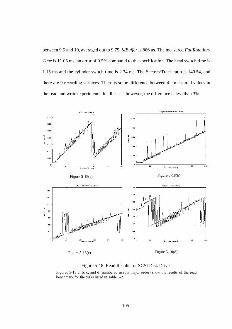
105
between 9.5 and 10, averaged out to 9.75. MBuffer is 866 us. The measured FullRotation-
Time is 11.05 ms, an error of 0.5% compared to the specification. The head switch time is
1.15 ms and the cylinder switch time is 2.34 ms. The Sectors/Track ratio is 140.54, and
there are 9 recording surfaces. There is some difference between the measured values in
the read and write experiments. In all cases, however, the difference is less than 3%.
Figure 5-18. Read Results for SCSI Disk DrivesFigures 5-18 a, b, c, and d (numbered in row major order) show the results of the readbenchmark for the disks listed in Table 5-2
Figure 5-18(a) Figure 5-18(b)
Figure 5-18(c) Figure 5-18(d)

106
The Seagate Barracuda’s result in Figure 5-18(b) is similar to model 5-16(b). Even though
Figure 5-16(b) illustrates an extreme case, we see that it can actually occur in disk drives.
Although Figure 5-16(b) shows only step sizes up to 250, we ran the experiment up to step
size 5000. The Barracuda chose to read all sectors between the current and the requested
sector. This causes the read latency to increase rapidly; even at step size 250, the latency
is already around 18 ms. The measured Mbuffer value is 970 us. The averaged Sbuffer
value is 12.75. The graph also shows occasional spikes caused by rotational misses. Even
though we could not extract FullRotationTime from Figure 5-18(b), we can find it from the
Barracuda result because of the rotational misses. The measured Rl value is 8.34 ms, a
0.1% error from the specification. The Sectors/Track ratio is 125. The head switch time is
0.73 ms. The graph does not show any noticeable cylinder switches, therefore we cannot
measure the cylinder switch time or the number of recording surfaces.
DiskMBuffer(ms)
FullRotationalLatency(ms)
MinimumTime toMedia (ms)
Sectors/Track(outermost)
NumberofRecordingSurfaces
HeadSwitchTime (ms)
CylinderSwitchTime (ms)
Hawk (5400) 0.87 11.05 2.11 140.54 9 1.15 2.34
Barracuda(7200)
0.97 8.34 - 125.04 21 0.73 -
Micropolis(7200)
- 8.40 3.19 206.66 22 1.31 2.97
UltraStar(7200)
0.47 8.44 2.46 182 18 0.84 2.23
9ZX (10020) 0.13 5.96 2.76 227.22 12 0.60 1.72
Table 5-4. Parameters Extracted from Read Benchmark
Table 5.4 lists the extracted parameters from each SCSI disk drive. The parameters for theIBM UltraStar XP disk are included for comparison. The MinimumMediaTime of theSeagate Barracuda cannot be determined because of its abnormal result.

107
Figure 5-18(c) shows that the 9ZX’s read behavior is similar to that of the UltraStar XP.
The MBuffer value is 130 us; the Sbuffer value averages out to 11.75. The measured rota-
tion time is 5.96 ms, a 1.7% error compared to the specification. The sectors/track ratio is
227, and the head and cylinder switch times are 0.6 ms and 1.7 ms respectively. The
number of recording surfaces is 12.
Finally, Figure 5-18(d) shows the read behavior of the Micropolis disk. This drive does not
seem to benefit from read ahead the way that the other drives do It’s read behavior is quite
similar to its write behavior. The measured rotation time is 8.40 ms, a 0.8% error compared
to the specification. The sectors/track ratio is 206.7, and the head and cylinder switch times
are 1.31 ms and 2.97 ms. The graph also shows that the disk has 22 recording surfaces.
5.7.2. IDE Disk Drives
Next we look at the read results for the IDE drives. Figure 5-19(a) shows the read result
for the IBM IDE drive; the graph is similar to model 5-16(a). MBuffer is 392 us and SBuffer
is 11.25. The measured FullRotationTime is 11020.15 us, a 0.8% error compared to the
specification. The measured values of HeadSwitchTime and CylinderSwitchTime are
1891.38 us and 3812.52 us respectively. The Sectors/Track ratio is 329.84 and the disk has
6 recording surfaces.
Figure 5-19(b) shows the result for the Quantum IDE drive; the graph matches the model
result in figure 5-14. The measured FullRotationTime is 11.35, a 2.3% error compared to
the specification. The Sectors/Track ratio is 360, and the head and cylinder switch times
are 2.14 ms and 2.84 ms respectively. The graph also shows that the disk has only two
recording surfaces.
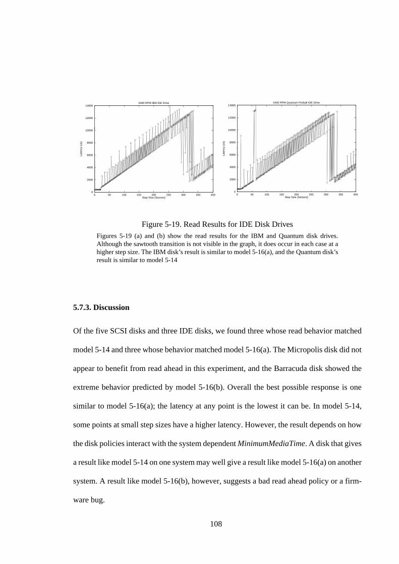
108
5.7.3. Discussion
Of the five SCSI disks and three IDE disks, we found three whose read behavior matched
model 5-14 and three whose behavior matched model 5-16(a). The Micropolis disk did not
appear to benefit from read ahead in this experiment, and the Barracuda disk showed the
extreme behavior predicted by model 5-16(b). Overall the best possible response is one
similar to model 5-16(a); the latency at any point is the lowest it can be. In model 5-14,
some points at small step sizes have a higher latency. However, the result depends on how
the disk policies interact with the system dependent MinimumMediaTime. A disk that gives
a result like model 5-14 on one system may well give a result like model 5-16(a) on another
system. A result like model 5-16(b), however, suggests a bad read ahead policy or a firm-
ware bug.
Figure 5-19. Read Results for IDE Disk DrivesFigures 5-19 (a) and (b) show the read results for the IBM and Quantum disk drives.Although the sawtooth transition is not visible in the graph, it does occur in each case at ahigher step size. The IBM disk’s result is similar to model 5-16(a), and the Quantum disk’sresult is similar to model 5-14
0
2000
4000
6000
8000
10000
12000
14000
0 50 100 150 200 250 300 350 400
Late
ncy
(us)
Step Size (Sectors)
5400 RPM IBM IDE Drive
0
2000
4000
6000
8000
10000
12000
14000
0 50 100 150 200 250 300 350 400
Late
ncy
(us)
Step Size (Sectors)
5400 RPM Quantum Fireball IDE Drive
109
Also, if we compare the SCSI and IDE disk results, we see that the IDE disks have lower
MBuffer values than almost all the SCSI disks. This is not surprising, as the IDE disks also
have much lower MinimumMediaTime values than the SCSI disks. The exception is the
SCSI 9ZX disk, which has a MBuffer of 130 us, a factor of two lower than all the other
disks.
5.8. Summary
Disks have always been difficult to measure because of the rotational effect. The rotational
latency can add anywhere from zero to the full rotation time to any latency measurement.
If we do not know what part of the latency is rotational, it is virtually impossible to deter-
mine other parameters like head switch time. This variability is why many benchmarks that
work on other parts of computer systems, like memory [Saavedra92, McVoy96[, do not
work well on disks. The linear stride technique actually takes advantage of the disk’s rota-
tional nature; the result curve shows very clearly what part of each measurement latency is
rotational. It is possible to extend this technique to filter out the rotational effect in all kinds
of disk measurements.
The Skippy benchmark strides across the disk, transferring one sector at a time and increas-
ing the step size with each step. The resulting latency curve has a sawtooth form; the lowest
points are the minimum latency to access drive media, and the highest points are when a
full rotational miss occurs. Instances of head and cylinder switches stand out clearly,
making it easy to determine switching times and the number of heads on the disk. This

110
single benchmark can extract all the disk geometry information and many useful mechan-
ical latencies.
We explored the benchmark behavior for writes and reads and presented results for seven
modern disk drives. We found that the write curves have the same shape for all disks, while
the read curves can have several shapes depending on the disk’s read ahead algorithms.
Nevertheless, we were able to extract parameters from all the write cases and all but one
of the read cases. The extracted parameters matched all the specification data we were able
to find, with less than 3% error. One of the benchmark’s strengths is that most parameters
can be measured in more than one way. Therefore, even if the shape of the curve changes
slightly between disks, we can still extract all the information we need.
In the next chapter, we explore extensions to the benchmark and presents a tool to automate
the parameter extraction process.
111
6 Automatic Extraction
6.1. Introduction
Chapter 5 described the Skippy algorithm for extracting disk geometry details and mechan-
ical latencies. The extracted information can be used by disk controllers, device drivers and
file system layers to create drive specific performance enhancements [Horst99]. Even
though the technique is simple and efficient, it cannot be incorporated into such a higher
level system without a mechanism to automatically extract the parameters from the graph-
ical result. This chapter describes such a mechanism.
The chapter is organized as follows. Section 6.2 describes the four phase approach used in
the extraction algorithm for write graphs. Section 6.3 describes each phase in detail and
illustrates the results on the IBM UltraStar XP disk drive. Once the technique has been
explained, we extract the parameters of the other SCSI disks in Section 6.4. Section 6.5
explores ways to improve the accuracy of the extracted results. Section 6.6 discusses these
results in more detail. Section 6.7 describes how the extraction techniques can be adapted
to read graphs and Section 6. 8 concludes with a summary. All through the chapter, the
SCSI disk results from Chapter 5 are used to test the extraction algorithms.
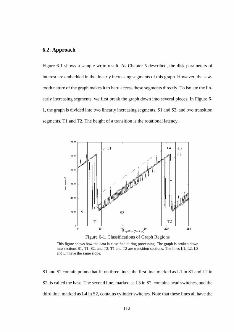
112
6.2. Approach
Figure 6-1 shows a sample write result. As Chapter 5 described, the disk parameters of
interest are embedded in the linearly increasing segments of this graph. However, the saw-
tooth nature of the graph makes it to hard access these segments directly. To isolate the lin-
early increasing segments, we first break the graph down into several pieces. In Figure 6-
1, the graph is divided into two linearly increasing segments, S1 and S2, and two transition
segments, T1 and T2. The height of a transition is the rotational latency.
S1 and S2 contain points that fit on three lines; the first line, marked as L1 in S1 and L2 in
S2, is called the base. The second line, marked as L3 in S2, contains head switches, and the
third line, marked as L4 in S2, contains cylinder switches. Note that these lines all have the
Figure 6-1. Classifications of Graph RegionsThis figure shows how the data is classified during processing. The graph is broken downinto sections S1, T1, S2, and T2. T1 and T2 are transition sections. The lines L1, L2, L3and L4 have the same slope.
T1 T2
S2S1
L1
L2
L3L4
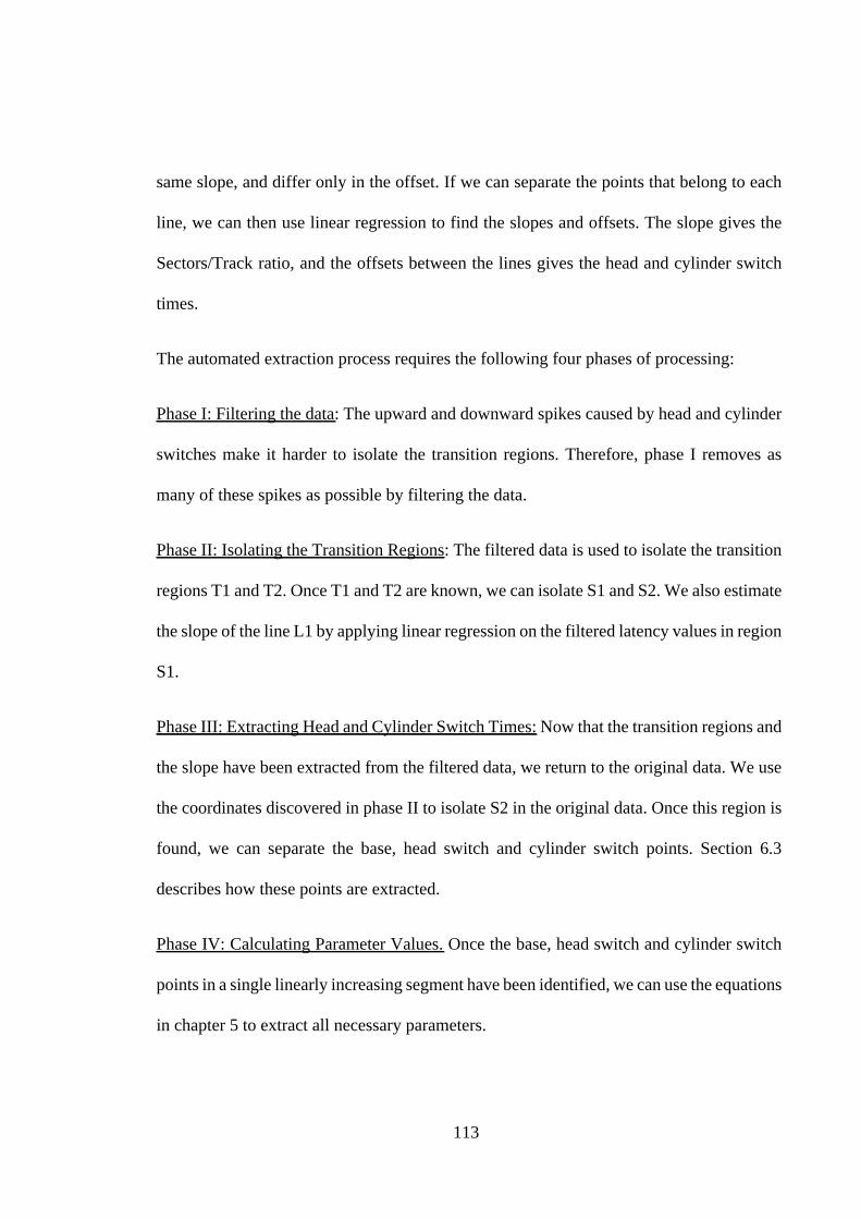
113
same slope, and differ only in the offset. If we can separate the points that belong to each
line, we can then use linear regression to find the slopes and offsets. The slope gives the
Sectors/Track ratio, and the offsets between the lines gives the head and cylinder switch
times.
The automated extraction process requires the following four phases of processing:
Phase I: Filtering the data: The upward and downward spikes caused by head and cylinder
switches make it harder to isolate the transition regions. Therefore, phase I removes as
many of these spikes as possible by filtering the data.
Phase II: Isolating the Transition Regions: The filtered data is used to isolate the transition
regions T1 and T2. Once T1 and T2 are known, we can isolate S1 and S2. We also estimate
the slope of the line L1 by applying linear regression on the filtered latency values in region
S1.
Phase III: Extracting Head and Cylinder Switch Times: Now that the transition regions and
the slope have been extracted from the filtered data, we return to the original data. We use
the coordinates discovered in phase II to isolate S2 in the original data. Once this region is
found, we can separate the base, head switch and cylinder switch points. Section 6.3
describes how these points are extracted.
Phase IV: Calculating Parameter Values. Once the base, head switch and cylinder switch
points in a single linearly increasing segment have been identified, we can use the equations
in chapter 5 to extract all necessary parameters.

114
6.3. Implementation Details
This section describes how each phase is implemented. Throughout the section, we use the
UltraStar XP’s graphical result to illustrate the processing steps. Some steps use techniques
borrowed from other fields, in particular the Artificial Intelligence and Statistics commu-
nities. Therefore, in each phase, we describe the techniques used, define any necessary
terms, and outline any trade-offs.
6.3.1. Phase I: Median Filter
The goal of phase I is to ease the detection of transition regions by removing as many spikes
as possible from the data. A median filter is very useful for this task, as it removes sudden
noise spikes without excessively distorting the surrounding data.
A median filter is a nonlinear filter commonly used in digital image processing to remove
noise from images [Davies88, Pitas90, Russ95]. In the digital processing context, a median
filter is a sliding window spatial filter that replaces each pixel with the median value of all
the pixels surrounding it. The advantage of the median filter is that it removes Gaussian
nose without affecting edges; a low pass filter, in contrast, will blur the image while reduc-
ing nose. Figure 6-2 shows a two dimensional median filter where the median is calculated
from the 3x3 grid surrounding the image. The number of points used to find the median is
the window size. In our context, we use a one dimensional version of the same idea. Figure
6-2 also shows a one dimensional filters with a window size of 5.

115
Figure 6-3 shows what happens when a median filter is applied to the benchmark result for
the IBM UltraStar XP drive. The original benchmark result is in Figure 6-1. The median
filter used here has window size 3; each latency value is replaced by the median of itself,
the value immediately before, and the value immediately after. We discuss the effects of
varying the window size later in the chapter. If we compare Figure 6-3 to Figure 6-1, we
can see that the graph in Figure 6-3 is considerably smoother for small step sizes. As long
as the step size is small, there are very few head and cylinder switches; once this region is
filtered, all those spikes are removed. The filter also causes the sawtooth transition to be
more clearly defined. At larger step sizes, there are too many head switches to be removed
by the median filter. However, we see that the filter smooths out the early part of the graph
and the first two transition regions quite well.
6.3.2. Phase II: Identifying the line slope and transition points
Now, we can use the filtered result to find the first two transition regions. Although the
median filter does a good job of removing noise spikes, we cannot guarantee that there will
be only one downward transition; therefore we identify transition regions in the graph. We
define a transition region to be when the latency drops from the prior value by over 30%.
Figure 6-2. Examples of Median FiltersThis figure shows a 3x3 window filter and a 5x1 median filter.
5 3 8
7 2 9
6 1 4
5→ 5 4 2 1 3 3→
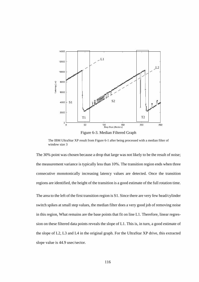
116
The 30% point was chosen because a drop that large was not likely to be the result of noise;
the measurement variance is typically less than 10%. The transition region ends when three
consecutive monotonically increasing latency values are detected. Once the transition
regions are identified, the height of the transition is a good estimate of the full rotation time.
The area to the left of the first transition region is S1. Since there are very few head/cylinder
switch spikes at small step values, the median filter does a very good job of removing noise
in this region, What remains are the base points that fit on line L1. Therefore, linear regres-
sion on these filtered data points reveals the slope of L1. This is, in turn, a good estimate of
the slope of L2, L3 and L4 in the original graph. For the UltraStar XP drive, this extracted
slope value is 44.9 usec/sector.
Figure 6-3. Median Filtered Graph
The IBM UltraStar XP result from Figure 6-1 after being processed with a median filter ofwindow size 3
S1
T1
S2
T2
L1
L2

117
6.3.3. Phase III: Identifying the head and cylinder switches
Next, we focus on the data segment between the two transition regions, region S2. We
cannot use this region in the filtered graph, however, since the median filter has removed
many cylinder and head switch points. Therefore, we analyze this region in the original
data. The median filtered data is used only to find the slope, the full rotation time, and the
transition regions.
Our goal is to classify each point in this region into one of three categories: base, head
switch, and cylinder switch. This is hard to do, however, because the latency values are lin-
early increasing. So we begin by removing the linearly increasing portion of the latency.
Since the full rotation time, Rl, is known, we can add it to each latency value in S2. This
causes the entire segment to move up, as in Figure 6-4(a). The base line in segment S2 now
becomes a continuation of line L1 from segment S1. Since we know the slope and offset of
line L1, we can subtract the linearly increasing segment from all points in region S2. Once
this is done, the data appears as in Figure 6-4(b); all the points in one category are now the
same height and the base, head switch and cylinder switch points are easily distinguishable.
Now that all the points from each category have roughly the same Y value, we can use a
clustering algorithm to separate the base, head switch and cylinder switch points. There is
a slight complication, however. Excess noise and unexpected rotational misses can create
points that don’t belong in any of the three categories. If these points are included in one of
the clusters, the outlying values will reduce the accuracy of the linear regression and the
extracted mechanical latency values.
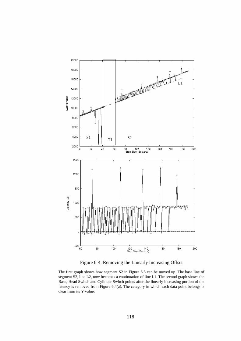
118
Figure 6-4. Removing the Linearly Increasing Offset
The first graph shows how segment S2 in Figure 6.3 can be moved up. The base line ofsegment S2, line L2, now becomes a continuation of line L1. The second graph shows theBase, Head Switch and Cylinder Switch points after the linearly increasing portion of thelatency is removed from Figure 6.4(a). The category in which each data point belongs isclear from its Y value.
S1T1 S2
L1

119
Our initial solution to this problem is as follows: the number of clusters is not set to three,
we impose only a minimum distance between clusters. This way, outlier points will form
clusters that will not be merged with the useful data points. Since we assume that there are
more useful data points than outliers, the three clusters with the most points will be the data
clusters. The key is choosing the right minimum distance so that head switch points and
cluster switch points are not merged into the same cluster. For the moment, we set the dis-
tance between clusters to 0.2 ms. Although this constant works well for the UltraStar XP
result, it is not a robust solution. Section 6.4 shows how well the constant works for other
cases and Section 6.5 explores more robust techniques.
6.3.4. Phase IV: Parameter calculation
Once the three clusters of points are identified, we can apply linear regression (using the
original latency values of each point), to calculate the head switch time HeadSwitchTime
and the cylinder switch time CylinderSwitchTime. Since we already know the slope Full-
RotationTime/SectorsPerTrack and we have an estimate of FullRotationTime, we can cal-
culate the Sectors/Track ratio. By counting the number of head switch data points between
each cylinder switch data point, we can calculate the number of recording surfaces.
6.3.5. A Sample Result
Table 6-1 shows the manufacturer specified parameters for the UltraStar XP drive, along
with the manually extracted and automatically extracted values.

120
The automatically extracted values are as follows. The full rotation time, measured as the
height of the transition, is 8.27 ms. Compared to the manufacturer’s specification, the error
is 0.7%. The sectors/track ratio is 184.18; the error is less than 0.1%. The head and cylinder
switch times are 0.87ms and 2.24ms respectively. The error rates here are 2.3% and 3.2%.
We see that the extracted values are very close to the actual values. In all cases, the error is
less than 5%. The table shows that the automatically extracted values differ slightly from
the manually extracted values. Occasionally, as in the Sectors/Track measurement, the
automatically extracted value is closer to the specified value than the manually extracted
value.
Parameter ManufacturerData
ManuallyExtractedValues
PercentageError (as com-pared to Man-ufacturerData)
AutomaticallyExtractedValues
PercentageError (as com-pared to Man-ufacturerData)
Sectors/Track 184 181.9 1.1% 184.2 0.1%
Full RotationTime
8.33 ms 8.30 ms 0.4% 8.27 ms 0.7%
MinimumMedia Time
- 2.19 ms - 2.34 ms -
Head SwitchTime
0.85 ms 0.87 ms 2.3% 0.87 ms 2.3%
CylinderSwitch Time
2.17 ms 2.19 ms 0.9% 2.24 ms 3.2%
Table 6-1. Percentage Errors of Manual and Automatic Extraction
The table shows, for each parameter, the manufacturer specified value, the value manuallyextracted using Skippy, and the value automatically extracted using Skippy. For all param-eters, both the automatically extracted and manually extracted values are close to the man-ufacturer value. The biggest disparity between manual and automatically extracted valuesoccurs in the MinimumMediaTime parameter. This disparity is larger because this value isdetermined using one or two points, and is as such more prone to error than the other val-ues.

121
6.4. Experiments
Next we apply this algorithm to the write results for the other SCSI disk drives presented
in Chapter 5. Figure 6-5 shows, for each SCSI disk, the absolute relative error between the
manually extracted values and those extracted by the algorithm. In all cases, the techniques
described in section 6.3 were used, with the same constant values (30% drop required to
determine transition in Phase II and 0.2 ms fixed distance between clusters in Phase III).
As the figure shows, in most cases the error rate is less than 5%. In general, the error rates
for the Minimum Time to Media are greater than the error rates for all other parameters. This
happens because the MinimumMediaTime value is approximated as part of the transition
detection process; the other parameter values are considerably more accurate since they are
extracted from a larger number of points.
The only disk whose extracted values show a marked inaccuracy is the Micropolis drive.
There are several reasons for this. First, as Figure 5.4 showed, the Micropolis disk result
has more noise than the other SCSI disks’ results. A single pass of a median filter does not
remove all noise spikes. As a result, the rotational latency value and the slope values are
less accurate. This inaccuracy affects all other results, since these quantities are used to cal-
culate SectorsPerTrack, HeadSwitchTime and CylinderSwitchTime. Second, the transition
region is considerably wider than in the other results, leading to a less accurate Minimum-
MediaTime measurement. Third, we discover that the clustering technique described in sec-
tion 6.3 does not work well for the Micropolis drives. The clustering process terminates
prematurely, since the constant separation distance of 0.2 ms is inappropriate for a result
with as much noise as the Micropolis result. Although the clusters containing base and head
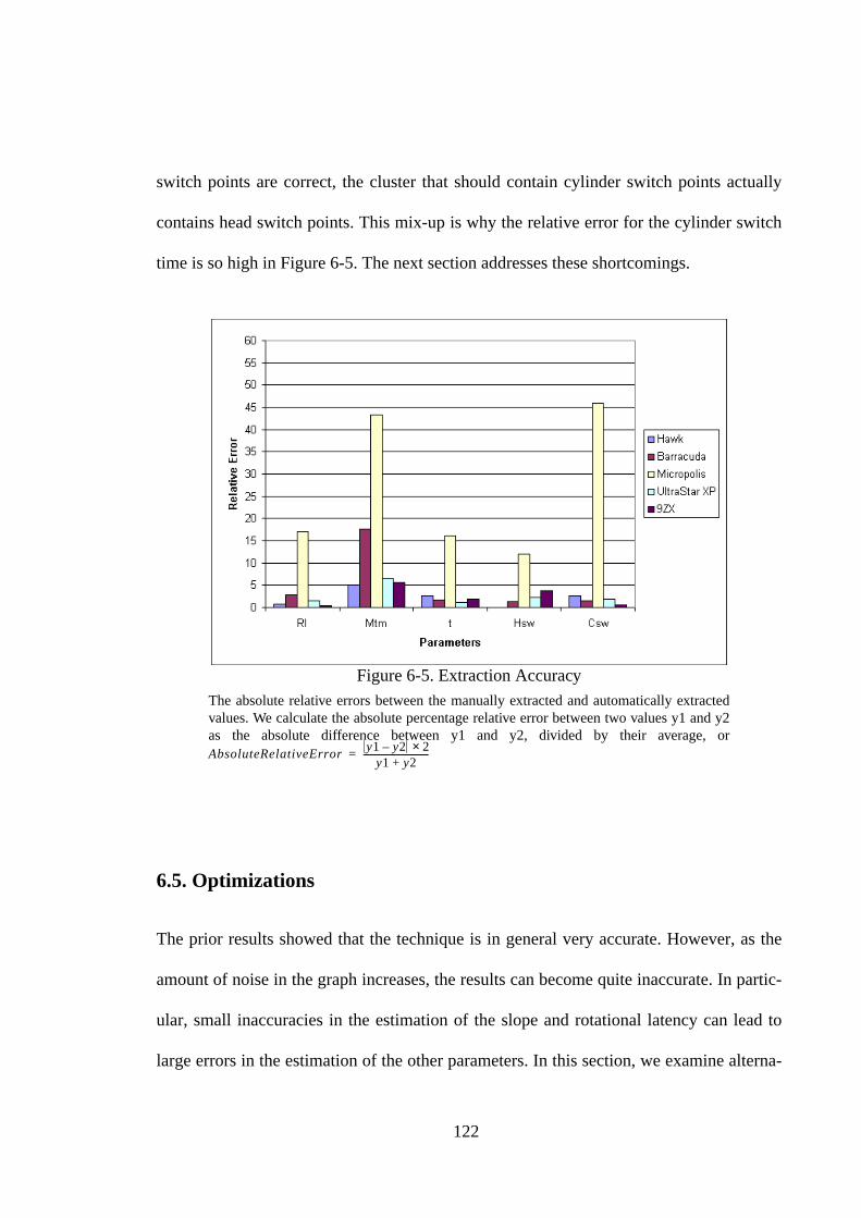
122
switch points are correct, the cluster that should contain cylinder switch points actually
contains head switch points. This mix-up is why the relative error for the cylinder switch
time is so high in Figure 6-5. The next section addresses these shortcomings.
6.5. Optimizations
The prior results showed that the technique is in general very accurate. However, as the
amount of noise in the graph increases, the results can become quite inaccurate. In partic-
ular, small inaccuracies in the estimation of the slope and rotational latency can lead to
large errors in the estimation of the other parameters. In this section, we examine alterna-
Figure 6-5. Extraction AccuracyThe absolute relative errors between the manually extracted and automatically extractedvalues. We calculate the absolute percentage relative error between two values y1 and y2as the absolute difference between y1 and y2, divided by their average, orAbsoluteRelativeError
y1 y2– 2×y1 y2+
------------------------------=

123
tives to the basic algorithm that deal with some of these problems. We explore the follow-
ing:
(i) Wider filters and multiple filter passes: The goal here is to reduce noise even fur-
ther by using filters with larger window sizes or using multiple passes of a filter.
The trade-off is that the data is further distorted.
(ii) Using an alternative clustering algorithm: The clustering algorithm used thus far
attempted to avoid outlier points by limiting the distance between clusters. Here we
explore alternative clustering algorithms.
(iii) Comparing multiple values of the same parameter for robustness checking: The
rotational latency and slope values are embedded in more than one place in the
graph. By comparing the values extracted from different points in the graph, we can
make some estimate of the accuracy of the extraction process.
We examine each optimization in turn, focusing on how the alternatives affect the extrac-
tion accuracy for the five disks mentioned in Section 6.4. Finally, we combine some of the
optimizations to create a better extraction algorithm.
6.5.1. Wider and Multiple Pass Filters
Figure 6-5 shows the extraction results when the data was filtered with one pass of a median
filter with window size 3. Here we examine four alternative filters: a size 5 filter, a size 7
filter, two passes of a size 3 filter, and three passes of a size 3 filter. Intuitively, a filter with
a smaller window distorts the data less than a filter with a larger window. At the same time,

124
a filter with a smaller window removes fewer spikes than a filter with a larger window.
Multiple passes of a smaller window filter will remove more spikes than a single pass,
while likely distorting the data less than a single pass of a filter with a larger window size.
Figure 6-6 shows the relative error rates for each parameter and each type of filter. In all
cases, the accuracy is calculated by comparing with the manually extracted value. In each
graph, the disks are labeled on the X-axis; each disk has a cluster of bars representing the
error rate with each filter. The filter’s are labeled on the legend, starting with the single
pass, size 3 filter, and ending with the single pass, size 7 filter.
In almost all the cases, we see that using multiple passes of the size 3 filter does not
increase the error. In the Micropolis case, where the errors are the highest and the data had
the most noise, the multiple passes give a noticeably improvement in the error rate. For
MinimumMediaTime, using two passes of the 3 filter reduces the error rate from over 40%
to around 25%. For FullRotationTime and Sectors/Track, the improvement is even greater.
The extra filtration does not help the accuracy of HeadSwitchTime and CylinderSwitch-
Time as much. This is not surprising; the head and cylinder switch times are affected more
by the clustering algorithm than the filtration process.
In most cases, using three passes of the 3 filter does not do damage, but also does not
improve the accuracy further. On the Micropolis result, the triple pass of 3 filter does cause
slightly higher error rates for FullRotationTime, SectorsPerTrack, HeadSwitchTime and
CylinderSwitchTime. It is still however, a great improvement from the single pass 3 filter.
The Barracuda is the only disk for which the three pass 3 filter seems to help; the error rates
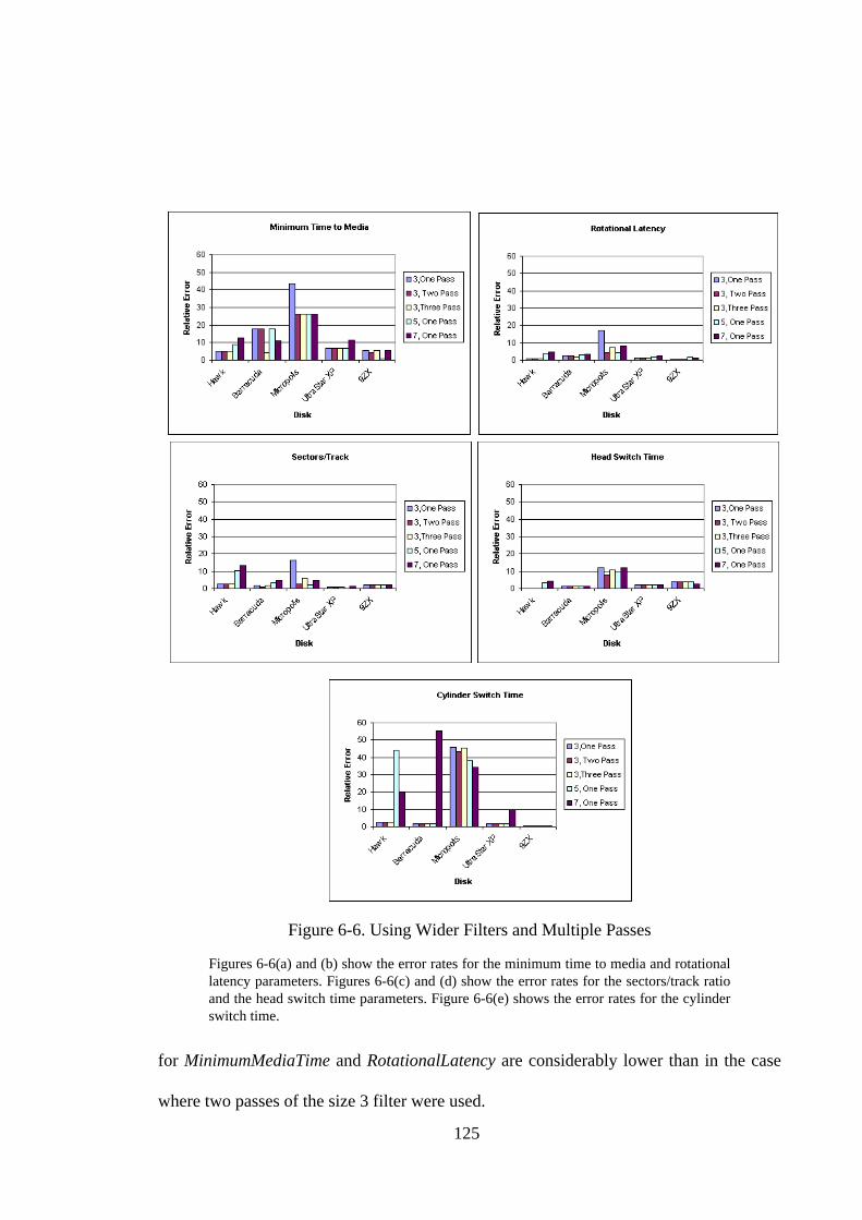
125
for MinimumMediaTime and RotationalLatency are considerably lower than in the case
where two passes of the size 3 filter were used.
Figure 6-6. Using Wider Filters and Multiple Passes
Figures 6-6(a) and (b) show the error rates for the minimum time to media and rotationallatency parameters. Figures 6-6(c) and (d) show the error rates for the sectors/track ratioand the head switch time parameters. Figure 6-6(e) shows the error rates for the cylinderswitch time.

126
The remaining two filters, the size 5 filter and size 7 filter, perform considerably worse
than the size 3 filters. In all cases but the Micropolis disk, these filters actually increase the
error rate. On the Micropolis, they do reduce the error compared to a single pass of the size
3 filter, but never do any better than two passes of the size 3 filter. Multiple passes of size
3 filters are less intrusive to the data than the size 5 and size 7 filters. Since the filter works
by replacing each value with the median of those around it, the size 5 and size 7 filters dis-
tort the data more than the size 3 filter. Our goal of removing point noise is better served
with multiple passes of the size 3 filter than with single passes of wider filters. Thus we
will use 2 passes of the size 3 filter as our baseline.
6.5.2. Using Alternative Cluster Algorithms
The clustering solution used so far in Phase III has been simple; points are grouped into
clusters until a minimum distance between clusters is reached. Although only three clusters
are expected, this technique stops noise points from joining the three clusters and affecting
the regression results. The distance between clusters was set to 0.2 ms; this value worked
well for all the graphs except the Micropolis disk. In that case, the algorithm stopped before
all the head switch points could be joined into one cluster. As a result, the points identified
by the algorithm to be cylinder switches were actually head switches. A better clustering
algorithm, one that does not require a fixed distance between clusters, is clearly needed.
While looking for a better clustering algorithm, we explored and rejected several alterna-
tives. We describe them briefly and explain why they did not work, but do not go into detail
with each. The unsuccessful alternatives are listed below:

127
(i) The first alternative was to force all points into three clusters and then remove
outliers from each cluster. This did not work because the values of the noise points
were so different from the data values that they tended to form clusters on their
own. As a result, the useful points were forced into a single cluster. The converse,
removing the outlier points before clustering, also does not work. If there are no
outliers, this process can remove cylinder switch data points.
(ii) The second alternative was to purposely place noise points that could attract
other noise points into clusters. Later, these noise clusters (identified by the artifi-
cial points), could be removed. Here we’re exploiting the fact that we can predict
the values of some outlier points. Given the structure of the graph, we expect some
outliers in the data with values of approximately plus and minus the rotational
latency. This technique worked well for some results. However, it is not robust
since it does not work when there are noise points with values far away from plus
and minus the rotational latency.
In the ideal case, the clustering should continue until most of the useful data is in the three
clusters, and stop before two of the useful clusters are merged into one. To effect this com-
promise, we used a hybrid technique. In the beginning, the clustering process proceeds
until the three largest clusters contain some predetermined percentage, p, of the data. After
this happens, we assume that each cluster has enough points that we can calculate its width
(the width is defined as the average plus or minus three times its variance). From this point
onwards, clusters are merged only when their widths overlap. The process stops once no
more clusters can be merged.

128
Figures 6-7(a) and (b) show the extracted head and cylinder switch times using this hybrid
optimization. Since the other parameters are extracted before the clustering phase, their
values do not change. Each figure shows the extraction accuracy for the original clustering
scheme and for the hybrid scheme for p=90% and p=95%. As the figures show, this tech-
nique does improve the accuracy of the extracted cylinder switch time for the Micropolis
disk. The accuracy of the head switch time is slightly worse on the Micropolis disk, but the
other disks’ results appear unaffected.
6.5.3. Using multiple extractions for accuracy checking
Because of the symmetric nature of the benchmark result, there are several ways to calcu-
late the FullRotationTime, and the slope FullRotationTime/SectorsPerTrack. In particular,
the latency value at step size 0 should be approximately FullRotationTime. The slope value
Figure 6-7. Using An Optimized Clustering Algorithm
Figures 6-7(a) and (b): Accuracy of head and cylinder switch values extracted using thenew cluster extraction algorithms. As the figures show, the new algorithm causes the headswitch error to increase slightly, but the cylinder switch error (for the Micropolis disk)improves dramatically.

129
is also available in more than one way. Once linear regression has been done on the base,
head switch, and cluster switch points, the slope values should be approximately equal, and
should also match the slope value extracted from the filtered graph. By comparing the
values of these parameters, we can obtain some assurance of the accuracy of the parameters
extracted by the algorithm.
6.5.4. Combining the optimizations: A better algorithm
This section combines the alternative filter and clustering options described above to create
a better extraction algorithm. The new algorithm uses two passes of a size 3 median filter
and the hybrid clustering algorithm described in section 6.5.2 with p=90%. Figure 6-8
shows the error rates of the resulting algorithm. If we compare these results to those of the
original extraction algorithm (in Figure 6-5), we see that the relative error rates of the opti-
mized algorithm are considerably lower. Except for the MinimumMediaTime values of the
Barracuda and Micropolis disk, and the CylinderSwitchTime value of the Micropolis disk,
the relative errors of all other parameters are less than 10%. In fact, the relative error of
most parameters is under 5%.
6.6. Discussion
Sections 6.4 and 6.5 show that an automated algorithm can successfully exact the critical
parameters embedded in the benchmark’s graphical result. In most cases, the automatically
extracted parameter values were within 5% of their manually extracted counterparts. The
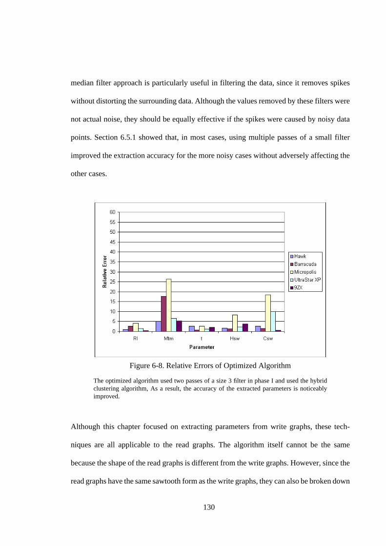
130
median filter approach is particularly useful in filtering the data, since it removes spikes
without distorting the surrounding data. Although the values removed by these filters were
not actual noise, they should be equally effective if the spikes were caused by noisy data
points. Section 6.5.1 showed that, in most cases, using multiple passes of a small filter
improved the extraction accuracy for the more noisy cases without adversely affecting the
other cases.
Although this chapter focused on extracting parameters from write graphs, these tech-
niques are all applicable to the read graphs. The algorithm itself cannot be the same
because the shape of the read graphs is different from the write graphs. However, since the
read graphs have the same sawtooth form as the write graphs, they can also be broken down
Figure 6-8. Relative Errors of Optimized Algorithm
The optimized algorithm used two passes of a size 3 filter in phase I and used the hybridclustering algorithm, As a result, the accuracy of the extracted parameters is noticeablyimproved.
131
into linearly increasing regions and transition regions. Since the head switch and cylinder
switch points are embedded in the linearly increasing segments of the read graphs, the tech-
niques described in section 6.3 and 6.5 should also work well for the read graphs.
6.7. Conclusion
This chapter outlined an algorithm for automatically extracting information embedded in
the graphical output of the Skippy benchmark. The algorithm was tested on the write
results of the five SCSI disks that were presented in Chapter 5. Several optimizations were
explored; combining the optimizations led to a new version of the extraction algorithm
whose results were in most cases within 5% of manual extraction.

132
7 Extensions
7.1. Introduction
The last two chapters presented the basic Skippy benchmark and a sample extraction tool.
The technique used single sector accesses, started with a step of 0, and increased the step
distance by one with each stride. This chapter describes extensions to this basic method.
The extensions take two forms. First, two algorithms are presented that, combined with
Skippy, extract a global picture of a disk drive by gathering information about recording
zones and seek behavior. The second part of the chapter describes how the Skippy tech-
nique can be extended by changing the step size interval and the transfer size. This section
also briefly introduces a backward stride technique that preserves the advantages of the
read Skippy technique while removing some disadvantages.
The chapter is organized as follows. Section 7.2 describes the two algorithms for collecting
zone and seek information and presents data for the disks described in Chapter 5. Section
7.3 describes how the basic technique can be extended with variable step size increments
and transfer sizes. Section 7.4 discusses related issues and Section 7.5 concludes with a
summary.

133
7.2. Extracting Global Disk Characteristics
The Skippy benchmark is local in nature; it provides a detailed picture of drive behavior
in a small area. Two global pieces that are missing are the drive’s recording zone charac-
teristics and its seek behavior. The recording zone characteristics describe how the Sectors/
Track ratio varies across different areas of the disk, and the seek behavior describes the
latencies associated with moving the disk arm.
7.2.1. Recording Zones
We begin with Zoned, a micro-benchmark designed to extract a bandwidth profile across
the different recording zones of the disk. The basic algorithm is depicted in Figure 7-1 and
is quite straight-forward. The algorithm reads each sector of the disk, in fixed size units.
The resulting graph of bandwidth vs. sector address shows the drive’s recording zones.
Note: it is possible to extract much the same information by sampling the bandwidth at var-
ious points in the disk drive. However, as the measurement results show, some disks are
very finely zoned: a full sweep is necessary to capture all the recording zones.
Figure 7-2 shows the algorithm’s result on the UltraStar XP disk drive. From the manufac-
turer specification, we learn that the disk has eight recording zones, with the Sectors/Track
ratio ranging from 184 at the outermost zone to 120 at the innermost zone. The graph
clearly shows the recording zones. Chapter 5 demonstrated how Skippy can extract Sec-
tors/Track in the local area where it is run. By running Skippy in each zone defined by
Figure 7-2, it is possible to extract Sectors/Track at each zone in the drive. Using this tech-
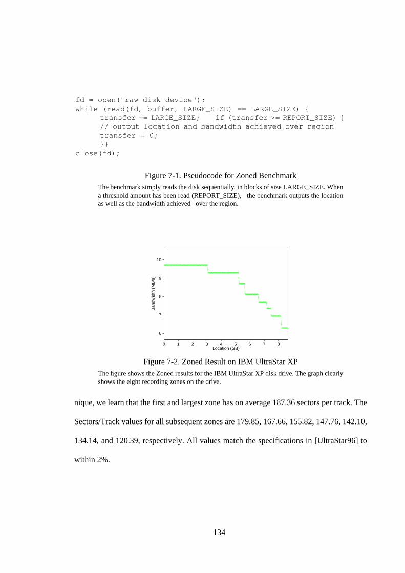
134
nique, we learn that the first and largest zone has on average 187.36 sectors per track. The
Sectors/Track values for all subsequent zones are 179.85, 167.66, 155.82, 147.76, 142.10,
134.14, and 120.39, respectively. All values match the specifications in [UltraStar96] to
within 2%.
Figure 7-1. Pseudocode for Zoned BenchmarkThe benchmark simply reads the disk sequentially, in blocks of size LARGE_SIZE. Whena threshold amount has been read (REPORT_SIZE), the benchmark outputs the locationas well as the bandwidth achieved over the region.
Figure 7-2. Zoned Result on IBM UltraStar XPThe figure shows the Zoned results for the IBM UltraStar XP disk drive. The graph clearlyshows the eight recording zones on the drive.
fd = open("raw disk device");while (read(fd, buffer, LARGE_SIZE) == LARGE_SIZE) {
transfer += LARGE_SIZE; if (transfer >= REPORT_SIZE) {// output location and bandwidth achieved over regiontransfer = 0;}}
close(fd);
6
7
8
9
10
0 1 2 3 4 5 6 7 8
Ban
dwid
th (
MB
/s)
Location (GB)

135
One also can observe the large difference in delivered bandwidth across the zones of the
drive. In the outermost zone, bandwidth is roughly 9.68 MB/s, whereas the inner tracks
deliver 6.29 MB/s, roughly a 54% increase from inner to outer tracks.
Figures 7-3(a) to 7-3(d) show the zoned results for the remaining SCSI disk drives. We can
make two general observations from these results. First, the Seagate drives are noticeably
more finely zoned than the IBM and Micropolis drives. Second, the overall difference
between outer-track and inner-track bandwidth ranges from 50% up to 80%. An anomaly
occurs with the Micropolis drive. The transfer rate at the outermost zones is lower than the
transfer rate in the next innermost zone. This anomaly is one of many oddities seen on the
Micropolis drive.
The most recent, comprehensive, discussion of disk drive zoning behavior was in
[VanMeter97], which observed that the relationship between transfer rate and disk position
was far better described with a linear function than a single value. After examining the zone
results, we see that the curve is actually closer to parabolic than linear. The quadratic shape
occurs partly because the outermost zone is often longer than the other zones. This feature
is particularly obvious in the IBM drives and occurs because an internal data rate limit is
reached and the drives cannot support a higher sectors per track ratio [Palmer99].
A quadratic function, of the form ax2 + b is a much better fit for the zone graph than the
linear function. In fact, by fitting both linear and quadratic functions to the data (using stan-
dard linear regression techniques), we learned that the quadratic function has between a
factor of 2 to a factor of 10 better error than the simple linear fit. The linear fit explored in
[VanMeter97] had an extra advantage in that it only required the highest and lowest band-
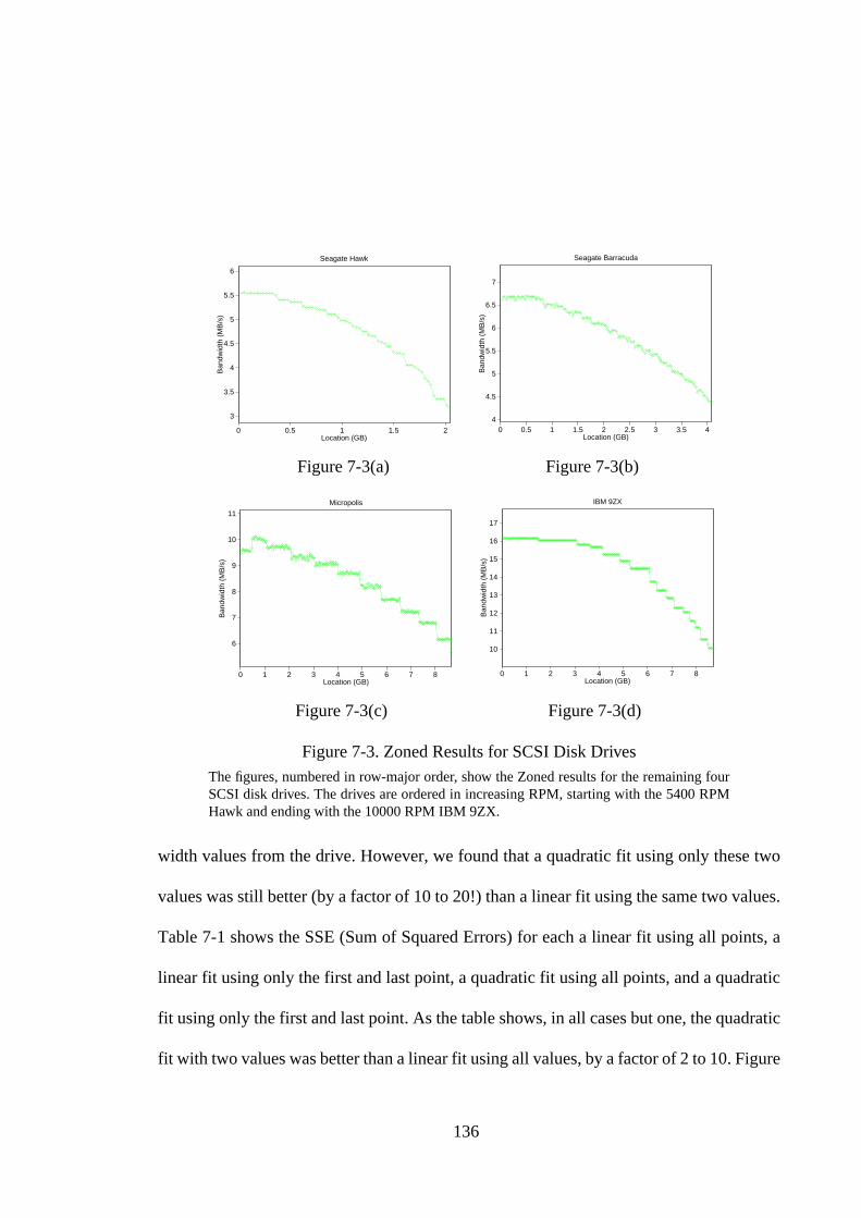
136
width values from the drive. However, we found that a quadratic fit using only these two
values was still better (by a factor of 10 to 20!) than a linear fit using the same two values.
Table 7-1 shows the SSE (Sum of Squared Errors) for each a linear fit using all points, a
linear fit using only the first and last point, a quadratic fit using all points, and a quadratic
fit using only the first and last point. As the table shows, in all cases but one, the quadratic
fit with two values was better than a linear fit using all values, by a factor of 2 to 10. Figure
Figure 7-3. Zoned Results for SCSI Disk DrivesThe figures, numbered in row-major order, show the Zoned results for the remaining fourSCSI disk drives. The drives are ordered in increasing RPM, starting with the 5400 RPMHawk and ending with the 10000 RPM IBM 9ZX.
Figure 7-3(a) Figure 7-3(b)
Figure 7-3(c) Figure 7-3(d)
3
3.5
4
4.5
5
5.5
6
0 0.5 1 1.5 2
Ban
dwid
th (
MB
/s)
Location (GB)
Seagate Hawk
4
4.5
5
5.5
6
6.5
7
0 0.5 1 1.5 2 2.5 3 3.5 4
Ban
dwid
th (
MB
/s)
Location (GB)
Seagate Barracuda
6
7
8
9
10
11
0 1 2 3 4 5 6 7 8
Ban
dwid
th (
MB
/s)
Location (GB)
Micropolis
10
11
12
13
14
15
16
17
0 1 2 3 4 5 6 7 8
Ban
dwid
th (
MB
/s)
Location (GB)
IBM 9ZX
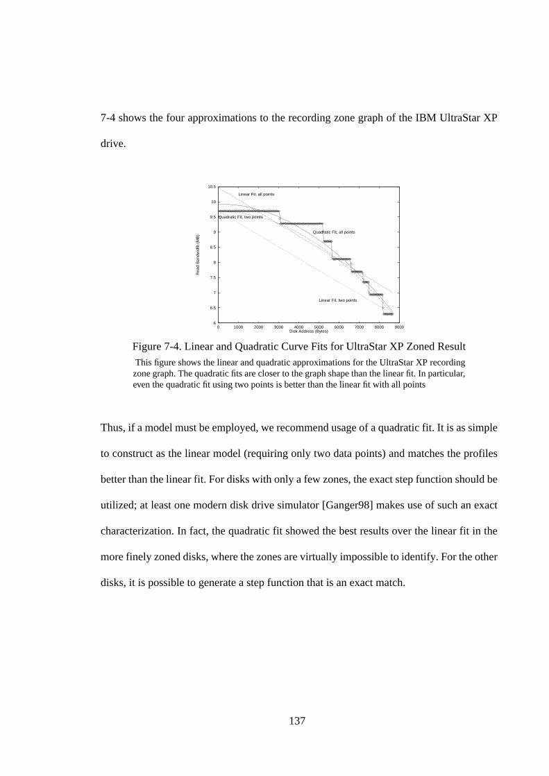
137
7-4 shows the four approximations to the recording zone graph of the IBM UltraStar XP
drive.
Thus, if a model must be employed, we recommend usage of a quadratic fit. It is as simple
to construct as the linear model (requiring only two data points) and matches the profiles
better than the linear fit. For disks with only a few zones, the exact step function should be
utilized; at least one modern disk drive simulator [Ganger98] makes use of such an exact
characterization. In fact, the quadratic fit showed the best results over the linear fit in the
more finely zoned disks, where the zones are virtually impossible to identify. For the other
disks, it is possible to generate a step function that is an exact match.
Figure 7-4. Linear and Quadratic Curve Fits for UltraStar XP Zoned Result This figure shows the linear and quadratic approximations for the UltraStar XP recordingzone graph. The quadratic fits are closer to the graph shape than the linear fit. In particular,even the quadratic fit using two points is better than the linear fit with all points
6
6.5
7
7.5
8
8.5
9
9.5
10
10.5
0 1000 2000 3000 4000 5000 6000 7000 8000 9000
Rea
d B
andw
idth
(M
B)
Disk Address (Bytes)
Linear Fit, all points
Linear Fit, two points
Quadratic Fit, all points
Quadratic Fit, two points

138
7.2.2. Seek Profile
The second global disk characteristic missing is the seek profile. Fortunately, seek delays
are based solely on the mechanical movements of the disk arm, and have been thoroughly
explored in several prior studies [Worthington95, Ruemmler91]. We limit our discussion
of seeks, therefore, to the following. First, we present a variant of Skippy that can be used
to make seek experiments easier by factoring out the rotational latency component of the
measured time. Second, we present seek curves as a function of sector distance, not cylin-
der distance.
Since Skippy is a local benchmark, it cannot be directly used to measure seek distances. If
the stride size is large, the benchmark will overrun the drive boundary before enough steps
are taken. Also, since the Sectors/Track ratio varies across different areas of the disk, the
striding technique is not useful when the strides cross a large portion of the disk surface.
However, we can utilize the technique to remove the rotational latency component of a
seek measurement.
Dri ve
SSE (Linear Fitusing all datapoints)
SSE(Linear Fitusing only twodata points)
SSE(QuadraticFit using alldata points)
SSE(QuadraticFit using twodata points)
Hawk 2.49 14.19 0.19 0.31
Barracuda 2.79 19.25 0.38 0.49
UltraStar XP 53.03 212.14 12.54 22.87
Micropolis 23.95 248.33 7.79 25.97
9ZX 156.88 795.05 30.72 99.67
Table 7-1. SSE for Linear and Quadratic Fits to Zoned Results
The table shows the Sum of Squared Errors for the linear and quadratic fits to the Zonedresults. The quadratic fit has less error, by between a factor of 2 to 10, than the linear fit inall cases. For all results but the Micropolis result, the quadratic fit using only two points isstill better, by factors of 2 to 10, than a linear fit using all data points.

139
Figure 7-5(a) describes an algorithm for measuring seek times. Between each of the mea-
surements, the algorithm writes to a fixed location at the beginning of the disk. This variant
allows the same disk space to be reused, and creates a similar (although not identical) saw-
tooth wave whose minimum value can be used to estimate the seek time if the rotational
latency is zero. By determining this minimum time for different seek distances, a seek pro-
file can be created.
The algorithm depicted in Figure 7-5 (a) uses write accesses. The second write in each iter-
ation can be replaced by a read, but the first write cannot. The reason is that the first write
is always to the same disk location. If it were replaced by a read, the read may be cached,
and the disk arm would not be moved to the starting location. Therefore, this algorithm
relies upon the drive not doing write caching.
A more robust algorithm, the Seeker algorithm, is described in Figure 7-5(b). In this case,
the disk accesses at each area of the disk are done with linear strides. This algorithm, in a
sense, is an interleave of two Skippy runs on different areas of the drive. This technique is
more robust since it works with reads as well as writes.
Figure 7-6 shows seek latency versus distance from sector 0 for the Seagate Barracuda. The
shape of the curve is slightly different from most seek curves seen in papers and textbooks,
since it is seek time versus sectors and not versus cylinders. Also note that the Minimal
Time to Media (Mtm) is included in the values reported; the true seek values can be
obtained by subtracting the Minimum Time to Media value derived by the Skippy bench-
mark.
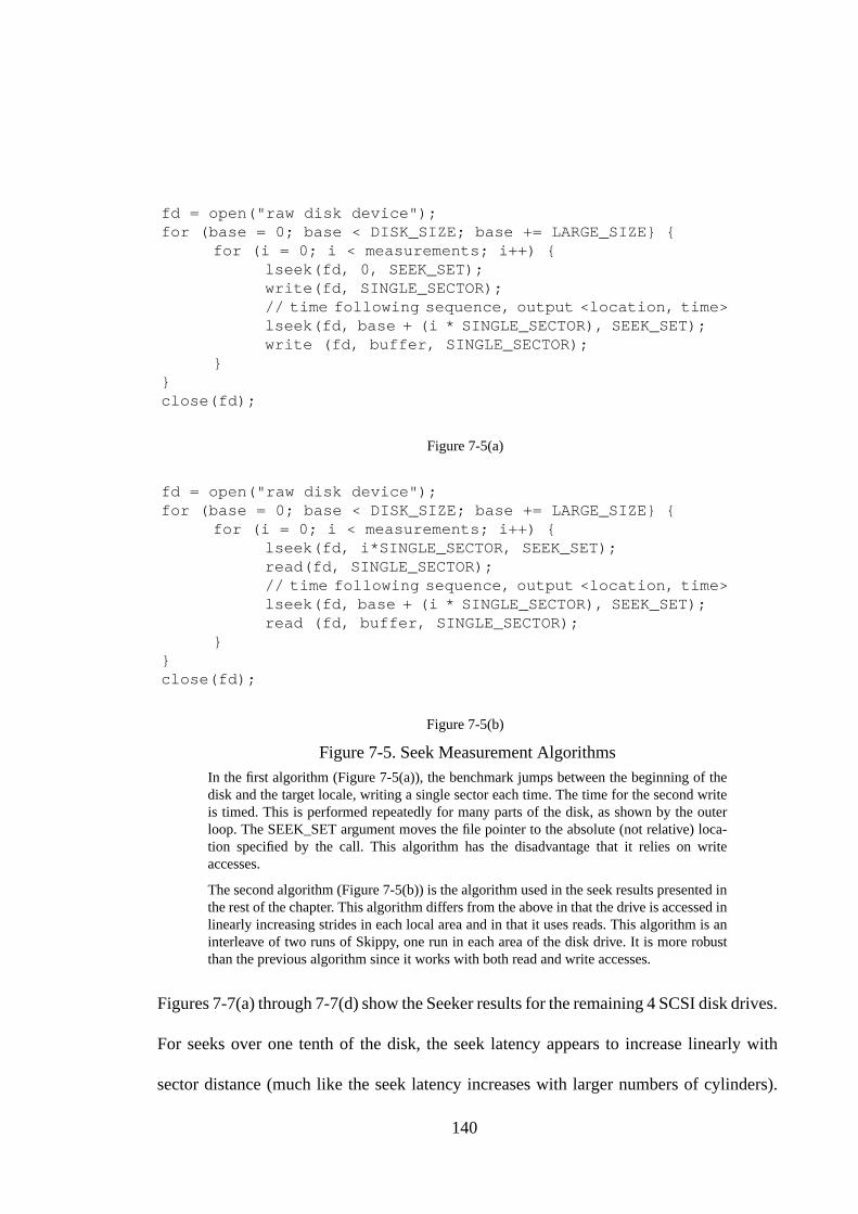
140
Figures 7-7(a) through 7-7(d) show the Seeker results for the remaining 4 SCSI disk drives.
For seeks over one tenth of the disk, the seek latency appears to increase linearly with
sector distance (much like the seek latency increases with larger numbers of cylinders).
Figure 7-5. Seek Measurement AlgorithmsIn the first algorithm (Figure 7-5(a)), the benchmark jumps between the beginning of thedisk and the target locale, writing a single sector each time. The time for the second writeis timed. This is performed repeatedly for many parts of the disk, as shown by the outerloop. The SEEK_SET argument moves the file pointer to the absolute (not relative) loca-tion specified by the call. This algorithm has the disadvantage that it relies on writeaccesses.
The second algorithm (Figure 7-5(b)) is the algorithm used in the seek results presented inthe rest of the chapter. This algorithm differs from the above in that the drive is accessed inlinearly increasing strides in each local area and in that it uses reads. This algorithm is aninterleave of two runs of Skippy, one run in each area of the disk drive. It is more robustthan the previous algorithm since it works with both read and write accesses.
fd = open("raw disk device");for (base = 0; base < DISK_SIZE; base += LARGE_SIZE} {
for (i = 0; i < measurements; i++) {lseek(fd, 0, SEEK_SET);write(fd, SINGLE_SECTOR);// time following sequence, output <location, time>lseek(fd, base + (i * SINGLE_SECTOR), SEEK_SET);write (fd, buffer, SINGLE_SECTOR);
}}close(fd);
Figure 7-5(a)
fd = open("raw disk device");for (base = 0; base < DISK_SIZE; base += LARGE_SIZE} {
for (i = 0; i < measurements; i++) {lseek(fd, i*SINGLE_SECTOR, SEEK_SET);read(fd, SINGLE_SECTOR);// time following sequence, output <location, time>lseek(fd, base + (i * SINGLE_SECTOR), SEEK_SET);read (fd, buffer, SINGLE_SECTOR);
}}close(fd);
Figure 7-5(b)

141
Close examination of the data reveals that, for seeks reaching the innermost zones, the
latency increase is higher than linear. This increase is most observable in the IBM 9ZX
seek result. The seek time increases more rapidly because the Sectors/Track ratio decreases
more rapidly in this area, requiring more arm movement for the same sector distance.
7.3. Extending the Skippy Technique
This section discusses how the Skippy technique can be extended by varying step size
intervals and transfer sizes. By increasing the step size interval, it is possible to extract all
the parameters extracted by the original technique in less time, using less disk area. The
trade-off, however, is that as the step size increment becomes larger, the result graph loses
detail. By increasing the transfer size, it is possible to measure the transfer rate of the drive.
Each extension is illustrated using the UltraStar XP disk drive.
Figure 7-6. Seeker Result for Seagate Barracuda Drive
0
2
4
6
8
10
12
14
16
18
0 0.5 1 1.5 2 2.5 3 3.5
See
k T
ime
(ms)
Distance (GB)
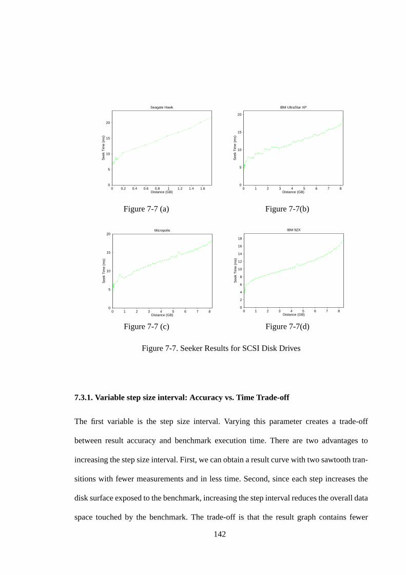
142
7.3.1. Variable step size interval: Accuracy vs. Time Trade-off
The first variable is the step size interval. Varying this parameter creates a trade-off
between result accuracy and benchmark execution time. There are two advantages to
increasing the step size interval. First, we can obtain a result curve with two sawtooth tran-
sitions with fewer measurements and in less time. Second, since each step increases the
disk surface exposed to the benchmark, increasing the step interval reduces the overall data
space touched by the benchmark. The trade-off is that the result graph contains fewer
Figure 7-7. Seeker Results for SCSI Disk Drives
Figure 7-7 (a) Figure 7-7(b)
Figure 7-7 (c) Figure 7-7(d)
0
5
10
15
20
0 0.2 0.4 0.6 0.8 1 1.2 1.4 1.6
See
k T
ime
(ms)
Distance (GB)
Seagate Hawk
0
5
10
15
20
0 1 2 3 4 5 6 7 8
See
k T
ime
(ms)
Distance (GB)
Micropolis
0
5
10
15
20
0 1 2 3 4 5 6 7 8
See
k T
ime
(ms)
Distance (GB)
IBM UltraStar XP
0
2
4
6
8
10
12
14
16
18
0 1 2 3 4 5 6 7 8
See
k T
ime
(ms)
Distance (GB)
IBM 9ZX

143
points, making the extracted values less accurate. Figures 7-8 (a) through (c) show the
benchmark’s write behavior for the IBM UltraStar XP disk, when the step size interval
varies from 1 to 3.
When the step size increment is 2 (Figure 7-8(b)), we see that some of the detail is lost, but
the graph retains all the important characteristics of Figure 7-8(a). Although there are fewer
points in this graph, there is enough information to extract all the necessary parameters. By
applying the automatic extraction technique, we get the following parameter values: the
Minimum Time To Media (Mtm) is 2.32ms, the FullRotationTime is 8.36ms, the Sectors/
Track ratio is 183.24, the head switch time is 8.70ms, and the cylinder switch time is 2.08
ms. Except for the cylinder switch time, all values are within 1% of their counterparts that
were extracted with step interval 1. The cylinder switch time value is within 7% of the orig-
inal; this value is less accurate because there are fewer points to contribute to the cylinder
switch time calculation. There are less head and cylinder switches overall, since the bench-
mark traverses less disk area. For this loss in accuracy, the gain is a reduced execution time.
While a single iteration with step size interval 1 took 1.57 seconds, an iteration with step
size interval 2 took 0.78 seconds.
If the step size interval is increased to 3, the graph deteriorates further. It is no longer pos-
sible to determine the cylinder switch time, since the benchmark does not travel across
more than one cylinder during a single sawtooth. Therefore, it does not make sense to
increase the step size interval beyond 2.
The main advantage to making the step size interval 2 is that the same parameters can be
extracted as in the original benchmark, while touching half the disk area. Since the original
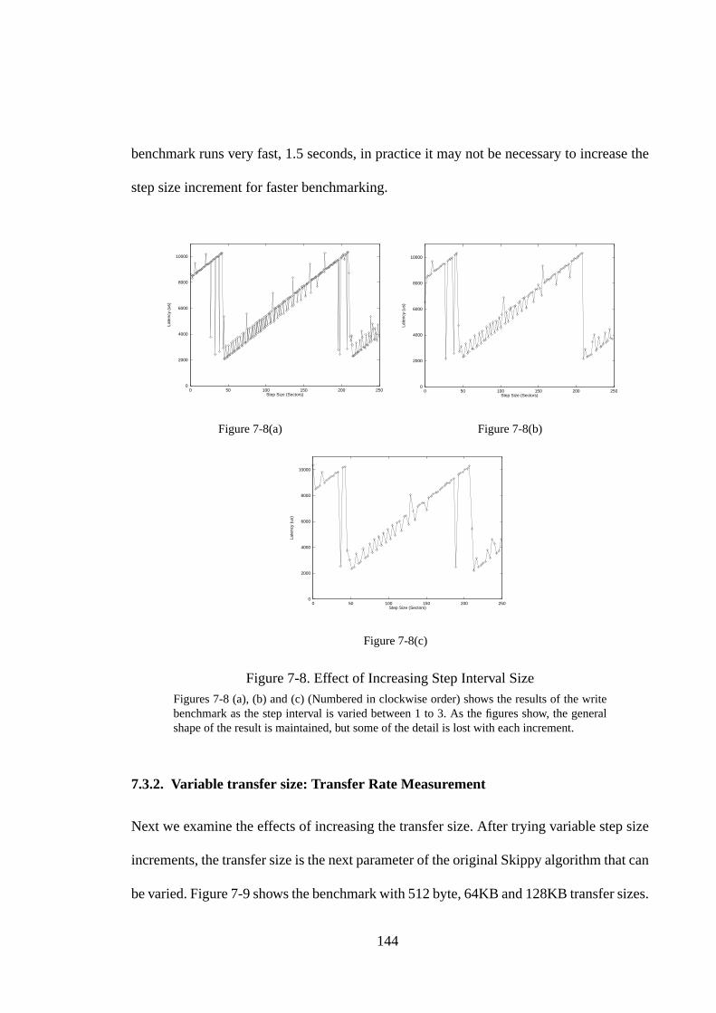
144
benchmark runs very fast, 1.5 seconds, in practice it may not be necessary to increase the
step size increment for faster benchmarking.
7.3.2. Variable transfer size: Transfer Rate Measurement
Next we examine the effects of increasing the transfer size. After trying variable step size
increments, the transfer size is the next parameter of the original Skippy algorithm that can
be varied. Figure 7-9 shows the benchmark with 512 byte, 64KB and 128KB transfer sizes.
Figure 7-8. Effect of Increasing Step Interval SizeFigures 7-8 (a), (b) and (c) (Numbered in clockwise order) shows the results of the writebenchmark as the step interval is varied between 1 to 3. As the figures show, the generalshape of the result is maintained, but some of the detail is lost with each increment.
0
2000
4000
6000
8000
10000
0 50 100 150 200 250
Late
ncy
(us)
Step Size (Sectors)
0
2000
4000
6000
8000
10000
0 50 100 150 200 250
Late
ncy
(us)
Step Size (Sectors)
0
2000
4000
6000
8000
10000
0 50 100 150 200 250
Late
ncy
(us)
Step Size (Sectors)
Figure 7-8(a) Figure 7-8(b)
Figure 7-8(c)
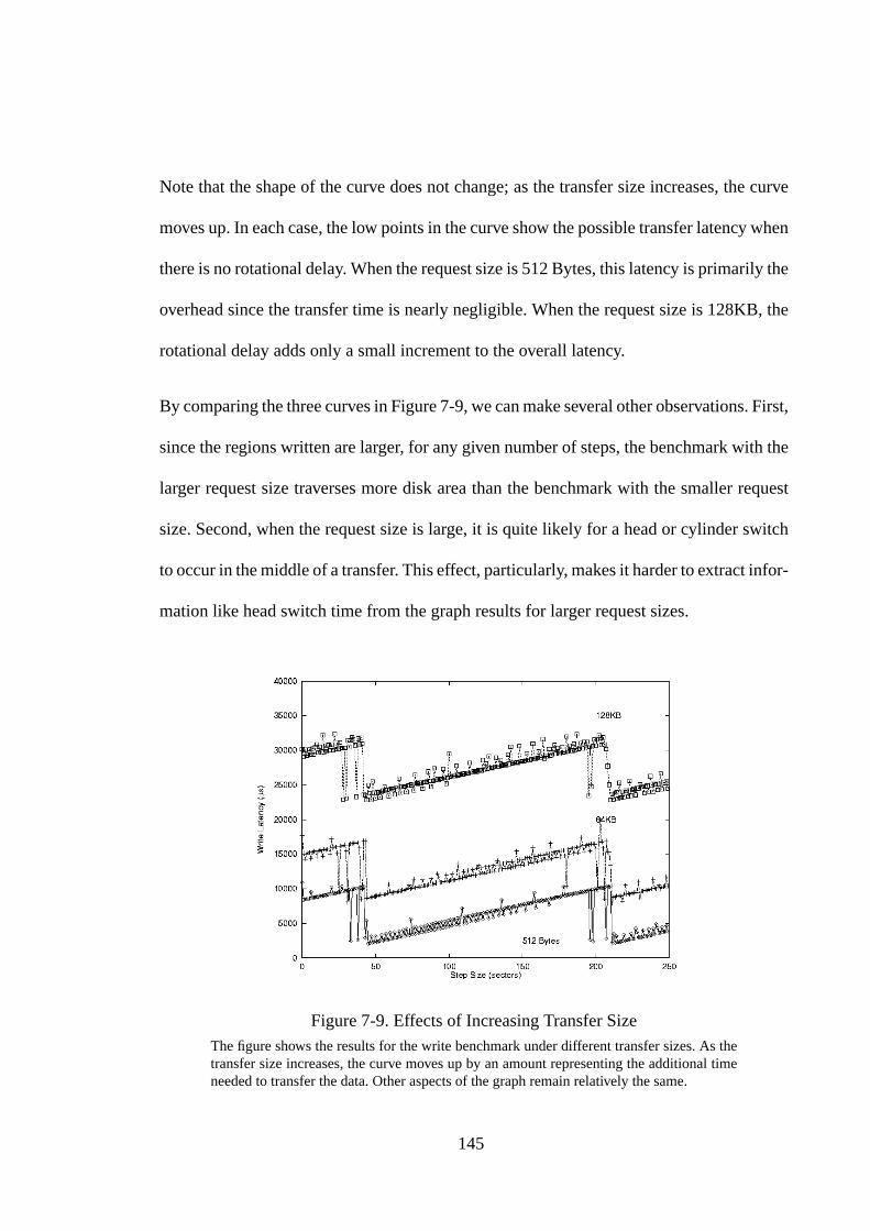
145
Note that the shape of the curve does not change; as the transfer size increases, the curve
moves up. In each case, the low points in the curve show the possible transfer latency when
there is no rotational delay. When the request size is 512 Bytes, this latency is primarily the
overhead since the transfer time is nearly negligible. When the request size is 128KB, the
rotational delay adds only a small increment to the overall latency.
By comparing the three curves in Figure 7-9, we can make several other observations. First,
since the regions written are larger, for any given number of steps, the benchmark with the
larger request size traverses more disk area than the benchmark with the smaller request
size. Second, when the request size is large, it is quite likely for a head or cylinder switch
to occur in the middle of a transfer. This effect, particularly, makes it harder to extract infor-
mation like head switch time from the graph results for larger request sizes.
Figure 7-9. Effects of Increasing Transfer SizeThe figure shows the results for the write benchmark under different transfer sizes. As thetransfer size increases, the curve moves up by an amount representing the additional timeneeded to transfer the data. Other aspects of the graph remain relatively the same.

146
These graphs are useful, primarily, for determining bandwidth. The request size divided by
the access latency gives the effective write bandwidth. Looking at the 128KB graph, we see
that when there is no rotational latency or head switch delay, access latency is approxi-
mately 23 ms, and the effective write bandwidth is approximately 5.57MB/s. In practice
however, a request will encounter some head switch delay and on average one half a full
rotational delay. When these effects are taken into account, the effective write bandwidth
becomes approximately 4.56MB/s. This value is close to the measured write bandwidth of
the disk, approximately 4.30MB/s.
7.3.3. The Backwards Read Benchmark
The final extension is the Backwards Read. Figure 7-10 shows the pseudocode for this
extension. Basically, the benchmark implements the Skippy technique in reverse, with read
accesses. Overall, the benchmark interacts with the drive mechanism in much the same
way that the forward benchmark does. At some point, the natural rotation between requests
matches the stride size, and the sawtooth transition occurs. The advantage of the backwards
read technique is that it maintains the advantages of read without the distortion of read
ahead. The backwards pattern is also less like regular access patterns, making it less sus-
ceptible to drive optimizations. Figure 7-11 shows the backwards read result on the IBM
UltraStar XP drive. The parameters extracted from this graph are also accurate, in all cases
within 4% of manufacturer specification.
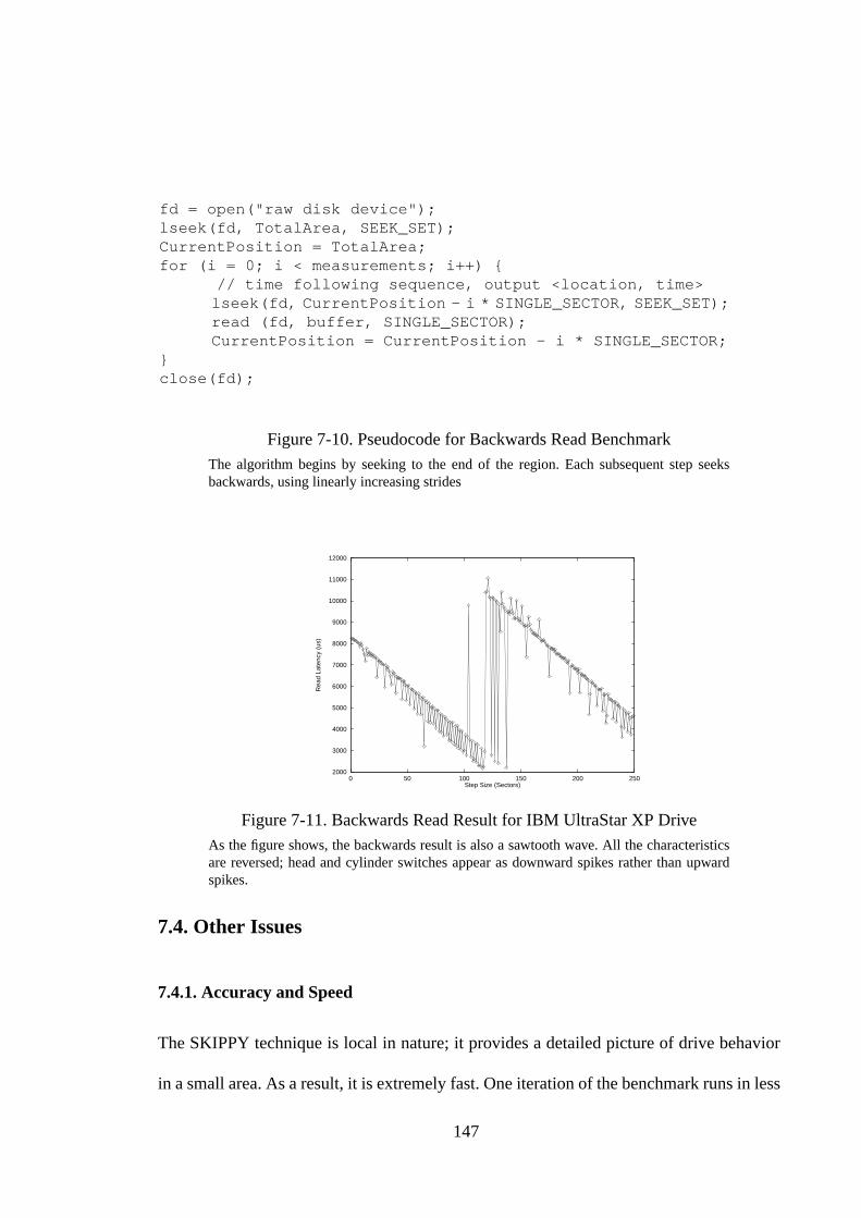
147
7.4. Other Issues
7.4.1. Accuracy and Speed
The SKIPPY technique is local in nature; it provides a detailed picture of drive behavior
in a small area. As a result, it is extremely fast. One iteration of the benchmark runs in less
Figure 7-10. Pseudocode for Backwards Read BenchmarkThe algorithm begins by seeking to the end of the region. Each subsequent step seeksbackwards, using linearly increasing strides
Figure 7-11. Backwards Read Result for IBM UltraStar XP DriveAs the figure shows, the backwards result is also a sawtooth wave. All the characteristicsare reversed; head and cylinder switches appear as downward spikes rather than upwardspikes.
fd = open("raw disk device");lseek(fd, TotalArea, SEEK_SET);CurrentPosition = TotalArea;for (i = 0; i < measurements; i++) {
// time following sequence, output <location, time>lseek(fd, CurrentPosition - i * SINGLE_SECTOR, SEEK_SET);read (fd, buffer, SINGLE_SECTOR);CurrentPosition = CurrentPosition - i * SINGLE_SECTOR;
}close(fd);
2000
3000
4000
5000
6000
7000
8000
9000
10000
11000
12000
0 50 100 150 200 250
Rea
d La
tenc
y (u
s)
Step Size (Sectors)
148
than a second on faster drives, such as 10000 RPM or 7200RPM, and in 2 to 3 seconds on
slower 5400 RPM drives. The accuracy of the extracted parameters is extremely good with
one iteration. Since it is good practice to perform multiple iterations, the data presented
here and in the last two chapters used 10 iterations of the benchmark. In practice, however,
there is no noticeable difference in accuracy between a measurement with 1 iteration or 10
iterations.
7.4.2. Cache Effects
Modern disks are capable of both read and write caching. In most SCSI disk drives that are
used in servers, write caching is disabled. Most IDE disk drives that are used in desktop
environments, write caching is enabled. When write caching is enabled, the write version
of SKIPPY does not work, since it is impossible to measure the latency of a write to disk
media. However, the read forward and read backwards versions do work on such disk
drives.
In the read cases, when Skippy uses forward strides, there is no need to flush the cache
between strides. Even between iterations, we did not find it necessary to flush the disk
buffer cache. By the time enough measurements are done in one iteration, the benchmark
has traversed about 20MB of disk area, so the data read during the first few accesses has
been flushed out of the cache.
The seek algorithms are far more sensitive to cache effects since they require the same disk
area to be repeatedly accessed. The first seek algorithm, presented in Figure 7-5(a) was
ineffective for this reason. The Seeker algorithm, presented in Figure 7-5(b), works despite
disk caching because it is essentially two runs of the Skippy benchmark. Within each local

149
area, the caching effects are the same as for a single run of Skippy. The backwards read
version can also be used in Seeker, resulting in yet a more robust seek algorithm.
7.5. Summary
This chapter described several extensions of the Skippy technique. The first half of the
chapter described Zoned and Seeker, two algorithms that can be used to extract global disk
drive characteristics. Zoned extracts the disk’s recording zones; the Sectors/Track ratio in
each zone can be found by running Skippy within the zone. Seeker measures the seek time
between two disk locations, using the linear stride technique to factor out the rotational
latency component. Automatic extraction would be useful for the Zoned result, to create a
table listing the starting and ending positions of each zone. The median filter technique is
also useful in this instance, for removing n oise. After the graph is filtered, it may be pos-
sible to isolate step transitions by determining gradient values within a small sliding win-
dow. We leave such an endeavor to future work.
The second half of the chapter described how Skippy can be used with different step size
increments and different transfer sizes. The advantage of increasing the step size increment
is that the same parameters can be extracted using less measurements, covering less disk
area, in less time. Experimentation showed that step increments of 2 are practical; the auto-
mated extraction algorithm can still extract the required parameters. Some accuracy is lost,
however, since there are fewer data points available. When the step size increment is raised
to 3, the resulting graph does not have enough information to extract all the required

150
parameters, although some values can still be extracted. When the transfer size is
increased, the result curve moves up. The base of the curve can be used to calculate the
drive’s transfer rate. The chapter also presented the Backwards Read technique that pre-
serves the advantages of reads and eliminates interaction with read ahead.
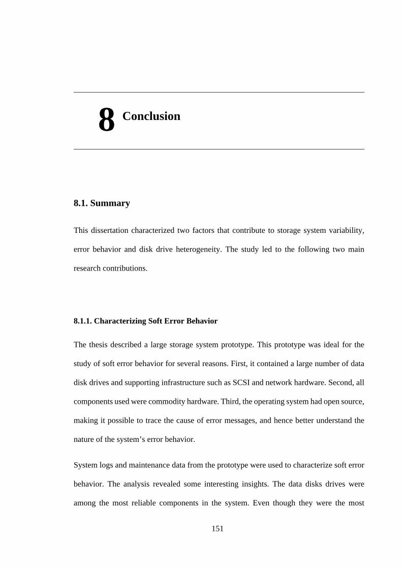
151
8 Conclusion
8.1. Summary
This dissertation characterized two factors that contribute to storage system variability,
error behavior and disk drive heterogeneity. The study led to the following two main
research contributions.
8.1.1. Characterizing Soft Error Behavior
The thesis described a large storage system prototype. This prototype was ideal for the
study of soft error behavior for several reasons. First, it contained a large number of data
disk drives and supporting infrastructure such as SCSI and network hardware. Second, all
components used were commodity hardware. Third, the operating system had open source,
making it possible to trace the cause of error messages, and hence better understand the
nature of the system’s error behavior.
System logs and maintenance data from the prototype were used to characterize soft error
behavior. The analysis revealed some interesting insights. The data disks drives were
among the most reliable components in the system. Even though they were the most
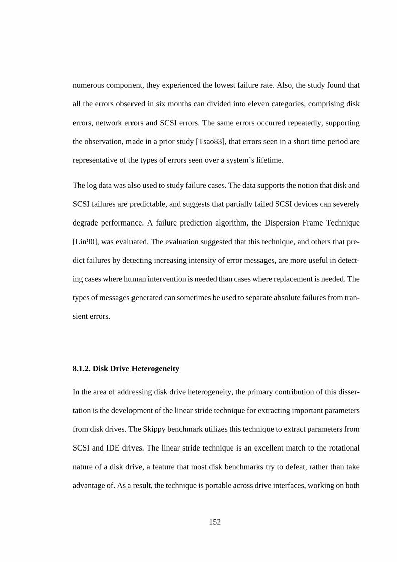
152
numerous component, they experienced the lowest failure rate. Also, the study found that
all the errors observed in six months can divided into eleven categories, comprising disk
errors, network errors and SCSI errors. The same errors occurred repeatedly, supporting
the observation, made in a prior study [Tsao83], that errors seen in a short time period are
representative of the types of errors seen over a system’s lifetime.
The log data was also used to study failure cases. The data supports the notion that disk and
SCSI failures are predictable, and suggests that partially failed SCSI devices can severely
degrade performance. A failure prediction algorithm, the Dispersion Frame Technique
[Lin90], was evaluated. The evaluation suggested that this technique, and others that pre-
dict failures by detecting increasing intensity of error messages, are more useful in detect-
ing cases where human intervention is needed than cases where replacement is needed. The
types of messages generated can sometimes be used to separate absolute failures from tran-
sient errors.
8.1.2. Disk Drive Heterogeneity
In the area of addressing disk drive heterogeneity, the primary contribution of this disser-
tation is the development of the linear stride technique for extracting important parameters
from disk drives. The Skippy benchmark utilizes this technique to extract parameters from
SCSI and IDE drives. The linear stride technique is an excellent match to the rotational
nature of a disk drive, a feature that most disk benchmarks try to defeat, rather than take
advantage of. As a result, the technique is portable across drive interfaces, working on both
153
SCSI and IDE drives, requires no prior knowledge of the drive’s internals, and delivers
extremely accurate results with a few seconds.
The thesis also describes an automated technique for extracting parameter values from the
graphical benchmark result. These techniques make it possible to use the linear stride tech-
nique, not merely as a stand-alone benchmark, but also has part of a larger adaptive storage
system. In such a system, the parameters of a new disk drive can be determined automati-
cally and used in disk specific optimizations or load balancing algorithms.
8.2. Future Directions
The results presented suggest future directions in both of the explored areas. The possible
future directions fall into two categories: ways to refine the characterization techniques,
and ways to make use of them in adaptive storage systems.
8.2.1. Understanding Error Behavior
In this dissertation, the analysis of soft error behavior was done by compiling statistics on
each type of observed error, understanding its cause by tracing the path of the error through
the operating system code, and by isolating failure cases and studying them in depth.
Although these techniques revealed many useful insights, there are several areas that
deserve further exploration:
154
(i) The logs provided empirical evidence that disk failures affect the performance of neigh-
boring disk drives. It would be useful to quantify the extent to which performance of neigh-
boring drives deteriorates. This data will help determine how to trade-off maintenance time
for system performance.
(ii) The logs showed evidence of correlations between events. For instance, network errors
were heavily correlated. It may be possible to apply data mining techniques to the system
log data to automatic detect interesting correlations.
(iii) The study of failure cases suggested that failure prediction algorithms are useful for
detecting cases where human intervention is required. The type of message can indicate
whether the failure is absolute or transient. A useful task for future work will be to deter-
mine how these two techniques can be combined in a failure detection and diagnostic sys-
tem.
8.2.2. Understanding Disk Drive Heterogeneity
This dissertation showed how linearly increasing strides can be used for extracting disk
drive parameters via operating system level measurements. This technique can be explored
further in the following ways:
(i) Chapter 7 presented initial work on the Backwards Read benchmark. This variant is
interesting because it retains the advantages of a read experiment without interference from
the drive’s read ahead mechanism. Further exploration of this variant would be useful.
155
(ii) Extending the linear stride technique to arrays of disk drives. Extracting critical param-
eters from disks in a striped array is also a useful exercise. A direction for future work
would be to see how these techniques could be extended to work over striped arrays, to
extract information about each disk in the array.
(iii) Finally, the ultimate goal would be to incorporate such a technique into an adaptive
storage system. This would require developing algorithms that can take advantage of the
underlying disk parameters to improve performance. Several such algorithms exist
[Horst99] [Worthington94]. Making use of them in an adaptive storage system is an inter-
esting direction for future research.
8.3. Conclusion
This thesis presented evidence variability in storage systems. The data showed that large
storage systems can display considerably variability, either from degraded behavior or
from device heterogeneity. An essential part of an adaptive storage solution will be to
understand and react correctly to such variability. The contributions of this dissertation
should assist such a task.
156
Bibliography
[Asami98] Asami, S. “GridPix: A Method for Presenting Large Image FilesOver the Internet”. http://now.cs.berkeley.edu/Td/Papers/.
[Asami99] Asami, S. Talagala, N. Patterson, D. “Design of a Self MaintainingStorage System”. In Proceedings of the 1999 IEEE Symposium onMass Storage Systems. pages 222-234. March 1999.
[Burkhard93] Burkhard, W. Menon, J. “Disk Array Storage System Reliability.”In Proceedings of the 23rd International Symposium on FaultTolerant Computing, June 1993.
[BSD96] McKusik, M.K. The Design and Implementation of the 4.4BSDOperating System. Addison-Wesley, 1996.
[Davies88] Davies, E.R. “On the Noise Suppression and Image EnhancementCharacteristics of the Median, Truncated Median, and ModeFilters.” In Pattern Recognition Letters. Vol 7. Pages 87-97, 1988.
[FreeBSD97] FreeBSD Library Functions Manual, Version 2.2
[Ganger98] Ganger, G. Worthington, B. Patt, Y. “The DiskSim SimulationEnvironment Version 1.0 Reference Manual”. Technical ReportCSE-TR-358-98. Department of Electrical Engineering andComputer Science, University of Michigan, February 1998.
[Gibson92] Gibson, G. Redundant Disk Arrays: Reliable, Parallel, SecondaryStorage. The MIT Press, Cambridge Massachusetts, 1992.
[Gray90] Gray, J. “A Census of Tandem System Availability Between 1985and 1990.” In IEEE Transactions on Reliability. Vol 39. No 4.October 1990.
[Grochowski96] Grochowski, E. Hoyt, R. “Trends in Modern Disk Drives”. IEEETransactions on Magnetics. vol.32, (no.3, pt.2) pages 1850-1854,May 1996.

157
[Horst99] Horst, B. MacDonald, J. Alessi, B. “Beyond RAID: AnArchitecture for Improving PC Fault Tolerance and Performance.”In Digest of Fast Abstracts, Proceedings of the 29th InternationalSymposium on Fault Tolerant Computing.
[IBM99] IBM Disk Drive Specifications, available at http://www.storage.ibm.com/.
[IDEMA97] Frank, B. “Rigid Disk Drive Price Trends.” IDEMA Insight. August1997.
[Kodak97] Flashpix White Paper. Kodak Corporation. http://www.kodak.com/country/US/en/digital/flashPix/.
[Lin90] Lin, T-T., Siewiorek, D. “Error Log Analysis: Statistical Modelingand Heuristic Trend Analysis.” In IEEE Transactions on Reliability.Vol 39. No 4. October 1990.
[Manley97] Manley, S., Seltzer, M. “Web Facts and Fantasy” In Proceedings ofthe 1997 USENIX Symposium on Internet Technologies andSystems, December 1997.
[McVoy96] McVoy, L. Staelin, C. “lmbench: Portable Tools for PerformanceAnalysis.” In Proceedings of the 1996 Winter USENIX Symposium.January 1996.
[Merry98] Merry, K. FreeBSD SCSI Group. Personal Communication.
[Ng94] Ng, S. Crosshatch Disk Array for Improved Reliability andPerformance. In Proceedings of the 21st International Symposiumon Computer Architecture. Pages 225-264. April 1994.
{Palmer99] Palmer, J. IBM Almaden Research. Personal Communication.
[PFA99] Predictive Failure Analysis. IBM Corporation. http://www.storage.ibm.com/storage/oem/tech/pfa.html.
[Pitas90] Pitas, I, Venetsanopoulos, A.N. Nonlinear Digital Filters:Principles and Applications. Kluwer academic publishers 1990.
[Quantum99] Quantum Disk Drive Specifications, available at http://www.quantum.com/.
[Ruemmler91] Ruemmler, C., Wilkes, J. An Introduction to Disk Drive Modeling.In IEEE Computer. March 1991.
[Russ95] Russ, J.C. The Image Processing Handbook, 2nd Edition. CRCPress 1995.
158
[Saavedra92] Saavedra-Barrera, R. CPU Performance Evaluation Using NarrowSpectrum Benchmarking. Ph.D Thesis, U.C. Berkeley, February1992.
[Saavedra94] Saavedra, R. Gaines, S. Carlton, M. “Characterizing thePerformance Space of Shared Memory Machines Using Micro-Benchmarks”, In Hot Interconnects 1994. August 1994.
[SCSI2] The SCSI-2 Interface Specification.
[Schwarderer96] Schwarderer, D., Wilson, D. Understanding I/O Subsystems.Adaptec Press, January 1996.
[Schulze88] Schulze, M.E. “Considerations in the Design of a RAID Prototype.”Technical Report UCB/CSD 88/448. Computer Science Division,University of California at Berkeley, 1988.
[Seagate99] Seagate Disk Drive Specifications, available at http://www.seagate.com.
[Sigma97] “SA-H381 Environmental Sensing CommunicationsSpecification.” Trimm Technologies, 1997.
[SMART99] “Self Monitoring, Analysis and Reporting Technology, FrequentlyAsked Questions.” Seagate Technology. http://www.seagate.com/support/disc/faq/smart.shtml
[Smith98] Smith, M. FreeBSD SCSI Group. Personal Communication.
[Talagala96] Talagala, N. Asami, S., Patterson, D. "A Comparison of PCOperating Systems for Storage Support." Technical Report UCB//CSD-98-1018. Computer Science Division, University ofCalifornia at Berkeley.
[Talagala99] Talagala, N. Asami, S., Patterson, D. "Usage Patterns of a WebBased Image Collection", In Proceedings of the 1999 IEEESymposium on Mass Storage Systems. March 1999.
[Tsao83] Tsao, M. “Trend Analysis and Fault Prediction.” PhD. Dissertation,Technical Report CMU-CS 83/130, Computer Science Division,Carnegie Mellon University, 1983.
[UltraStar96] “Ultrastar 2XP Hardware/Functional Specification: 4.55 GB and8.22 GB Models, 7200 RPM, Version 5.03.” Document NumberAS05-0087-45. IBM Storage Products Division. June 1996.
[VanMeter97] VanMeter, R. “Observing the effects of Multizone Disks.” InProceedings of the 1997 USENIX Conference, January 1997.
159
[Worthington94] Worthington, B.L., Ganger, G, Patt, Y. “Scheduling Algorithms ForModern Disk Drives.” In 1994 International Conference on theMeasurement and Modeling of Computer Systems. Pages 241-151.May 1994.
[Worthington95] Worthington, B.L., Ganger, G.R., Patt, Y.N., Wilkes, J. “On-lineExtraction of SCSI Disk Drive Parameters.” In 1995 JointInternational Conference on Measurement and Modeling ofComputer Systems.
[Yoshikawa97] Yoshikawa, C. Chun, B. Eastham, P. Vahdat, A. Anderson, T.Culler, D. “Using Smart Clients to Build Scalable Services”. InProceedings of the 1997 USENIX symposium.
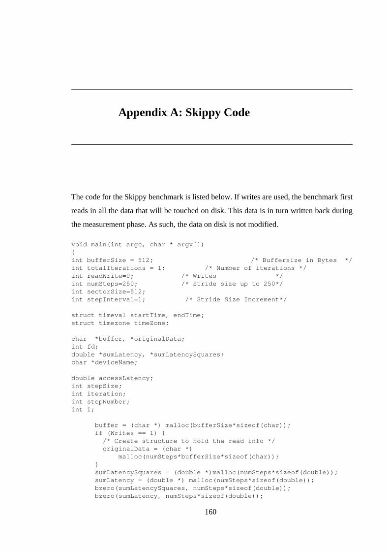
160
Appendix A: Skippy Code
The code for the Skippy benchmark is listed below. If writes are used, the benchmark first
reads in all the data that will be touched on disk. This data is in turn written back during
the measurement phase. As such, the data on disk is not modified.
void main(int argc, char * argv[]){int bufferSize = 512; /* Buffersize in Bytes */int totalIterations = 1; /* Number of iterations */int readWrite=0; /* Writes */int numSteps=250; /* Stride size up to 250*/int sectorSize=512;int stepInterval=1; /* Stride Size Increment*/
struct timeval startTime, endTime;struct timezone timeZone;
char *buffer, *originalData;int fd;double *sumLatency, *sumLatencySquares;char *deviceName;
double accessLatency;int stepSize;int iteration;int stepNumber;int i;
buffer = (char *) malloc(bufferSize*sizeof(char));if (Writes == 1) { /* Create structure to hold the read info */ originalData = (char *)
malloc(numSteps*bufferSize*sizeof(char));}sumLatencySquares = (double *)malloc(numSteps*sizeof(double));sumLatency = (double *) malloc(numSteps*sizeof(double));bzero(sumLatencySquares, numSteps*sizeof(double));bzero(sumLatency, numSteps*sizeof(double));
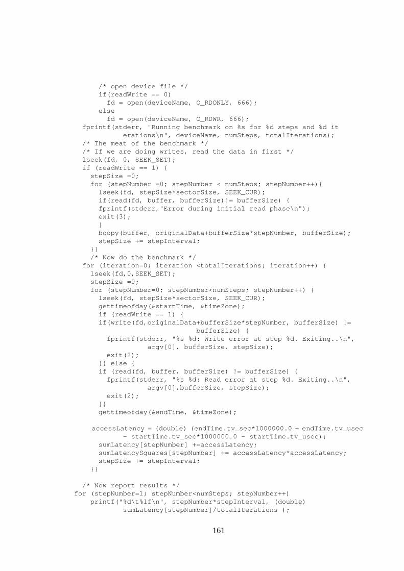
161
/* open device file */if(readWrite == 0) fd = open(deviceName, O_RDONLY, 666);else fd = open(deviceName, O_RDWR, 666);
fprintf(stderr, "Running benchmark on %s for %d steps and %d iterations\n", deviceName, numSteps, totalIterations);
/* The meat of the benchmark */ /* If we are doing writes, read the data in first */ lseek(fd, 0, SEEK_SET); if (readWrite == 1) { stepSize =0; for (stepNumber =0; stepNumber < numSteps; stepNumber++){ lseek(fd, stepSize*sectorSize, SEEK_CUR); if(read(fd, buffer, bufferSize)!= bufferSize) {
fprintf(stderr,"Error during initial read phase\n");exit(3);
} bcopy(buffer, originalData+bufferSize*stepNumber, bufferSize); stepSize += stepInterval; }} /* Now do the benchmark */ for (iteration=0; iteration <totalIterations; iteration++) { lseek(fd,0,SEEK_SET); stepSize =0; for (stepNumber=0; stepNumber<numSteps; stepNumber++) { lseek(fd, stepSize*sectorSize, SEEK_CUR); gettimeofday(&startTime, &timeZone); if (readWrite == 1) {
if(write(fd,originalData+bufferSize*stepNumber, bufferSize) !=bufferSize) {
fprintf(stderr, "%s %d: Write error at step %d. Exiting..\n",argv[0], bufferSize, stepSize);
exit(2);}} else {if (read(fd, buffer, bufferSize) != bufferSize) { fprintf(stderr, "%s %d: Read error at step %d. Exiting..\n",
argv[0],bufferSize, stepSize); exit(2);}}
gettimeofday(&endTime, &timeZone);
accessLatency = (double) (endTime.tv_sec*1000000.0 + endTime.tv_usec- startTime.tv_sec*1000000.0 - startTime.tv_usec);
sumLatency[stepNumber] +=accessLatency; sumLatencySquares[stepNumber] += accessLatency*accessLatency; stepSize += stepInterval; }}
/* Now report results */for (stepNumber=1; stepNumber<numSteps; stepNumber++) printf("%d\t%lf\n", stepNumber*stepInterval, (double)
sumLatency[stepNumber]/totalIterations );

162
/* Clean up and exit */close (fd);exit(0);}


