Characterization of Chimney Flue Gas Flows

Flow Rate Measurements with Averaging Pitot Probes

Janne Paavilainen

Ingår i rapportserier: Lic / Department of Civil and Environmental Engineering, Chalmers University of Technology Lic 2016:5, ISSN 1652-9146 ISSN 1401 - 7555 ISRN DU-SERC- -99- -SE May 2016

Högskolan Dalarna SE 791 88 Falun

Tel: +46 23 778000 www.du.se

Högskolan Dalarna SE 791 88 Falun

Tel: +46 23 778000 www.du.se

Licentiate Thesis

Janne Paavilainen

2016-05-03

Characterization of Chimney Flue Gas Flows Flow Rate Measurements with Averaging

Pitot Probes

ABSTRACT Performance testing methods of boilers in transient operating conditions (start, stop and combustion power modulation sequences) need the combustion rate quantified to allow for the emissions to be quantified. One way of quantifying the combustion rate of a boiler during transient operating conditions is by measuring the flue gas flow rate. The flow conditions in chimneys of single family house boilers pose a challenge however, mainly because of the low flow velocity. The main objectives of the work were to characterize the flow conditions in residential chimneys, to evaluate the use of the Pitot-static method and the averaging Pitot method, and to develop and test a calibration method for averaging Pitot probes for low 𝑅𝑅𝑅𝑅.

A literature survey and a theoretical study were performed to characterize the flow conditions in in single family house boiler chimneys. The flow velocities under normal boiler operating conditions are often below the requirements for the assumptions of non-viscous fluid justifying the use of the quadratic Bernoulli equation. A non-linear calibration coefficient is required to correct for these viscous effects in order to avoid significant measurement errors. The flow type in the studied conditions changes from laminar, across the transition regime, to fully turbulent flow, resulting in significant changes of the velocity profile during transient boiler operation. Due to geometrical settings occurring in practice measurements are often done in the hydrodynamic entrance region, where the velocity profiles are neither fully developed nor symmetrical. The predicted changes in velocity profiles are also confirmed experimentally in two chimneys.

Several requirements set in ISO 10780 and ISO 3966 for Pitot-static probes are either met questionably or not met at all, meaning that the methods cannot be used as such. The main issues are the low flow velocity, viscous effects, and velocity profiles that change significantly during normal boiler operation. The Pitot-static probe can be calibrated for low 𝑅𝑅𝑅𝑅, but is not reliable because of the changing velocity profiles.

The pressure averaging probe is a simple remedy to overcome the problems with asymmetric and changing velocity profiles, but still keeping low the irrecoverable pressure drop caused by the probe. However, commercial averaging probes are not calibrated for the characterized chimney conditions and the information available on the performance of averaging probes at low 𝑅𝑅𝑅𝑅 is scarce. A literature survey and a theoretical study were done to develop a method for calibrating pressure averaging probes for low 𝑅𝑅𝑅𝑅 flue gas flows in residential chimneys.

The experimental part consists of constructing a calibration rig, testing the performance of differential pressure transducers, and testing a prototype pressure averaging probe. The results show good correlation over a wide operation range, but the low 𝑅𝑅𝑅𝑅 characteristics of the probe could not be identified due to instability in the chosen pressure transducer, and temperature correlation for one of the probes while not for the other. The differential pressures produced are close to the performance limitations of readily available transducers and it should be possible to improve the method by focusing on finding or building a suitable pressure transducer. The performance of the averaging method can be improved further by optimizing the geometry of the probe. Another way of reducing the uncertainty would be to increase the probe size relative to the conduit diameter to produce a higher differential pressure, at the expense of increasing the irrecoverable pressure drop.

TABLE OF CONTENTS Abstract ................................................................................................................................................... 5 Table of Contents ................................................................................................................................... 7 1 Introduction ..................................................................................................................................... 1

1.1 Background ............................................................................................................................. 1 1.2 Aim and Scope ........................................................................................................................ 2 1.3 Method .................................................................................................................................... 3

2 The Pitot-Static Probe ..................................................................................................................... 5 2.1 Principle of operation ............................................................................................................. 5 2.2 Theory ...................................................................................................................................... 6 2.3 Calibration ............................................................................................................................... 7 2.4 Correction for Low Re – Stagnation Pressure Coefficient ................................................... 7

3 The Pitot-Static Method in Flue Gas Flow Rate Measurements ................................................ 10 3.1 ISO 10780 and ISO 3966 Requirements and Limitations ................................................ 10 3.2 Limitations in the Differential Pressure Measurement ...................................................... 12 3.3 Reported Issues .................................................................................................................... 12 3.4 Need for Development of Methods for Residential Boiler Chimney Conditions ............... 13

4 Chimney flow characteristics ....................................................................................................... 14 4.1 Residential Chimney Boundary Conditions ......................................................................... 14

4.1.1 Typical Boiler Installations ........................................................................................... 14 4.1.2 Physical and Combustion Data for Residential Boiler Operation .............................. 16 4.1.3 Chimney Diameters ...................................................................................................... 18 4.1.4 Characteristics of Boiler Operation ............................................................................. 19

4.2 Bulk Average Reynolds Number and Flow Type ................................................................. 21 4.2.1 The Reynolds Number .................................................................................................. 21 4.2.2 Critical Reynolds Number and Transition of Flow Type .............................................. 22 4.2.3 Reynolds Numbers and Flow Types in Residential Chimneys ................................... 22 4.2.4 Intermittency and Hysteresis of Flow Type Transition ................................................ 24

4.3 Flow Velocity Profiles ............................................................................................................ 25 4.3.1 Fully Developed Velocity Profiles ................................................................................. 25 4.3.2 Intermediate and Asymmetric Velocity Profiles .......................................................... 27 4.3.3 Hydrodynamic Entrance Region .................................................................................. 28 4.3.4 Single Point Velocity Measurement Methods ............................................................. 30 4.3.5 Measured Chimney Flow Velocity Profiles .................................................................. 31 4.3.6 Flow Conditioners ......................................................................................................... 34

4.4 Viscous Effects ..................................................................................................................... 34 4.4.1 Probe External Reynolds Number ................................................................................ 34 4.4.2 Probe Stagnation Pressure Port Reynolds Number ................................................... 36

4.5 Wall Proximity and Stem Blockage ...................................................................................... 37 4.6 Flue gas density .................................................................................................................... 38 4.7 Average flow temperature .................................................................................................... 38 4.8 Yaw angle .............................................................................................................................. 39 4.9 Vibrations .............................................................................................................................. 39 4.10 Turbulence ............................................................................................................................ 39 4.11 Differential Pressure ............................................................................................................ 40 4.12 Other considerations ............................................................................................................ 41

5 The Averaging Pitot Probe ............................................................................................................ 42 5.1 Principle of operation ........................................................................................................... 42 5.2 Theory .................................................................................................................................... 44

5.2.1 Definition of Reynolds Number for Cylinders .............................................................. 44 5.2.2 Pressure Coefficient And Its Distribution .................................................................... 45

5.3 Calibration ............................................................................................................................. 46 5.4 Correction for Low Re - Stagnation and Wake Pressure Coefficient ................................. 47

5.4.1 Stagnation Pressure Coefficient .................................................................................. 47 5.4.2 Wake Pressure Coefficient ........................................................................................... 48 5.4.3 Combined Stagnation and Wake Pressure Coefficient .............................................. 48

6 Prototype Averaging Pitot Probe .................................................................................................. 51 7 Differential Pressure Transducers ............................................................................................... 54

7.1 Background ........................................................................................................................... 54 7.2 Experimental Comparison of Pressure Transducers .......................................................... 54

7.2.1 Measurement Setup ..................................................................................................... 55 7.2.2 Resolution and Stability ............................................................................................... 55 7.2.3 Temperature Drift ......................................................................................................... 55 7.2.4 Hysteresis, Noise, Time constant ................................................................................ 56 7.2.5 Zero Level Adjustment - Automatic Zeroing ................................................................ 56 7.2.6 Other error sources ...................................................................................................... 57

8 Development of a Calibration Method ........................................................................................ 61 8.1 Experimental Equipment ...................................................................................................... 61 8.2 Calibration Theory................................................................................................................. 64

9 Testing of the Calibration Method ............................................................................................... 66 9.1 Data Sets .............................................................................................................................. 66 9.2 Quadratic Correlation ........................................................................................................... 70 9.3 Quadratic Correlation With Low Re Correction ................................................................... 73 9.4 Analysis of Inconsistent Results .......................................................................................... 73 9.5 Irrecoverable Pressure Drop Caused by the Probe ............................................................ 74

10 Discussion ..................................................................................................................................... 76 11 Conclusions ................................................................................................................................... 77

11.1 Chimney Flow Characteristics .............................................................................................. 77 11.2 Evaluation of the Pitot-static Method .................................................................................. 78 11.3 Evaluation of the Averaging Pitot Probe .............................................................................. 78 11.4 Differential Pressure Transducers ....................................................................................... 79 11.5 Development of a Calibration Method ................................................................................ 79

12 Future Work .................................................................................................................................. 81 12.1 Detailed Characteristics of Pressure Transducers ............................................................. 81 12.2 Detailed Characteristics of the Pressure Coefficients 𝑪𝑪𝑪𝑪𝑪𝑪 and 𝑪𝑪𝑪𝑪𝑪𝑪 .............................. 81 12.3 Optimization of Probe Cross Section ................................................................................... 81 12.4 Probe Response Dependency on the Fluid Flow Temperature ......................................... 82 12.5 Determining the Time Constant ........................................................................................... 82 12.6 Uncertainty Analysis ............................................................................................................. 82 12.7 Impact of Deposits ............................................................................................................... 82 12.8 Developing the Averaging Method Further for Field Measurements ................................ 83

13 Acknowledgments ........................................................................................................................ 84 14 Nomenclature ............................................................................................................................... 85 15 References .................................................................................................................................... 87

1

1 INTRODUCTION

1.1 BACKGROUND With the conversion from direct electrical and fossil fuel to bioenergy based heating systems there has been increasing interest in determining the efficiency, and characterizing and quantifying the emissions (e.g. carbon monoxide, hydrocarbons, nitric oxides, particles) of residential heating boilers (single- to multi-family house size), e.g. [1]–[3]. Arguments and evidence have been presented that the steady state testing methods of boilers, such as EN-303-5:2012 [4], do not represent the normal intermittent and transient operation (start, stop and combustion power modulation) of such boilers in real applications, e.g.[5]–[7]. Especially in the case of solid fuel boilers work has been done to develop methods for quantifying the efficiency and emissions on a yearly basis with a combination of transient simulations and boiler models validated by laboratory measurements [5], [8]–[11], with the further purpose of finding solutions to improve the systems.

For determining the combustion and flue gas flow rates a scale is normally used for measuring the solid fuel consumption of a burner. However, the amounts of fuel combusted during short transients are usually too small compared to the resolution and measurement errors of the scale to acquire data with reasonable uncertainty [8], [9].

When the fuel composition is known, the combustion rate can also be determined indirectly from the flue gas flow rate, combined with a flue gas composition analysis [5], [10], [12]. Such a method can also be used in field measurement studies where the use of a scale would be practically impossible. For both research and benchmark testing purposes it is thus beneficial to be able to do reliable continuous (i.e. logging data over longer periods) measurements of transient flue gas flow rates from single family house size heating boilers. However, the flow conditions in ducts and chimneys during normal boiler operation of these boilers are challenging from a measurement engineering point of view:

• The low flow velocities and geometrical conditions (flow disturbances) in the chimneys normally do not meet the requirements for Pitot-static probe measurements according to ISO 10780 and ISO 3966. Moreover, the standards do not readily provide methods for taking into account the various measurement error sources under these conditions.

• Methods causing higher irrecoverable pressure drops to the flow than the Pitot-static method would be significantly more accurate, but prevent realistic operation of the burner under natural draft conditions, and therefore cannot be used outside of laboratory environment.

• Clogging due to particulate deposits and condensation may cause measurement errors and thus the probe should be easy to clean frequently without disturbing the operation of the boiler and preserving the calibration of the probe.

A further problem with the Pitot-static method in low flow rates is the differential pressure measurement. Industrial standard pressure transducers are not calibrated for the range of differential pressures induced by a Pitot-static probe in residential chimney flows, which is in the same order of magnitude as the measurement uncertainties given by the manufacturers.

2

One way to improve the measurement uncertainty, without causing a high irrecoverable pressure drop, is by using an averaging Pitot-probe. The main advantages, compared to the Pitot-static method, are that skewed and changing velocity profiles are taken into account, and the differential pressure output is increased. These types of probes are commercially available since the 1960’s [13]. The problem, however, similarly to the Pitot-static method, is that the available probes are not calibrated for the low flow velocities present in residential chimneys, and the available information for adapting averaging method to these flow conditions is scarce.

It should be noted that the residential chimney conditions result in such low flow velocities, that they present a challenge in all the areas of theory, methodology, equipment, and practical handling of the equipment. The flow conditions are mainly identified by 𝑅𝑅𝑅𝑅𝐵𝐵𝐵𝐵𝐵𝐵 ≲ 10 000 (or 𝑣𝑣𝑅𝑅��� ≲3 m/s), with both varying flow rate and temperature. Fluid mechanical phenomena with such flow velocities have been studied both theoretically and experimentally in much detail during the last century, but are complex and difficult to generalize. In practice these problems are normally avoided by forcing the flow conditions to a state where the theory can be simplified and the uncertainties and limitations of the measurement equipment are of less concern. Therefore there is not much research done regarding developing practical Pitot-static or averaging methods and equipment specifically for low flow velocities in ducts or chimneys.

1.2 AIM AND SCOPE This work is a pre-study for developing a method for measuring the very low flow velocities present in residential boiler chimneys, without causing a high irrecoverable pressure drop to the flow. The need for this came during developing a test rig for comparative performance studies of single family house wood pellet boilers under transient conditions. The study is thus limited to chimneys for biomass boilers in single family houses, as the test rig was specifically developed for this.

The objective of this work was to:

• Characterize the chimney flow conditions of residential boilers for flow rate measurement methods based on differential pressure measurement.

• Evaluate the Pitot-static method in the characterized flow conditions. • Evaluate the averaging Pitot probe in the characterized flow conditions. • Develop a calibration method for the characterized flow conditions.

First the focus is on Pitot-static type probes as these are extensively studied, internationally standardized and widely used. Further, the focus is on the averaging Pitot probe, which is a further development of the Pitot-static method allowing for instantaneous sampling of the average velocity pressure over one or several diameters.

Other types of methods, such as orifice plates or venturi tubes, are not considered, as the main objective is to determine whether the Pitot-static method, or the averaging Pitot probe, are suitable for the task.

3

1.3 METHOD Characterization of the chimney flow conditions of residential boilers

A literature survey was done to summarize earlier work regarding Pitot-static measurement methods for fluid flows in closed conduits, with focus on low flow velocities. The area is widely researched and there is an extensive literature resource available. Thus to keep the reference list manageable, general summary type references are mostly preferred, and specialized sources regarding the topic of low flow velocities are referred to, where suitable.

Based on the literature survey theoretical studies were done, where the main purpose was to characterize the flow conditions in the specific case of residential boiler chimneys of single family houses. The results are presented and compared with literature in a manner that gives a general view to cover the wide operating ranges of various types of residential solid fuel boilers. The purpose is to evaluate the impact of predictable physical effects on flue gas flow rate measurements.

Flow velocity profile measurements in two laboratory test chimneys were performed and the results analyzed to confirm some of the phenomena found in the literature.

Evaluating the Pitot-static method in the characterized flow conditions

The limitations of the Pitot-static method are discussed in combination with the characterization of chimney flow conditions. The flow conditions are compared to the requirements set in the standards ISO 10780 and ISO 3966. The impact of the characteristic of each physical phenomenon and possible correction methods are discussed.

Evaluating the averaging Pitot method in the characterized flow conditions

The expected characteristics of the probes were studied theoretically based on literature to determine the needed correlations and corrections, with focus on modeling the characteristics with low 𝑅𝑅𝑅𝑅 flows.

Developing a calibration method for the characterized flow conditions

Two prototype averaging multi-port differential pressure probes for flue gas flow measurements in 80 mm and 100 mm internal diameter chimneys were constructed. The probes were designed specifically for laboratory measurements of flue gas flow rates from single family house heating boilers and stoves, but also considering the application to field measurement requirements of similar boilers

4

Three industrial standard differential pressure transducers were tested in the expected measurement range. Their performance and suitability were evaluated, with the purpose of finding a suitable candidate to be used in combination with the prototype averaging Pitot probe.

A calibration rig was developed and constructed to test the measurement method for the intended operating range regarding both flow and temperature. Focus was on developing a calibration rig where calibration reference uncertainty with the lowest expected flow rates is still within ±2 %.

Measurements were performed to determine the characteristics of the prototype probes, and the performance in combination with the chosen pressure transducer. Isotherm data sets with four temperature levels were acquired to derive the correlations and to evaluate eventual temperature dependency. Validation data sets with emulated inlet configuration changes and disturbances were acquired to evaluate their impact on uncertainty and repeatability.

5

2 THE PITOT-STATIC PROBE

Velocity pressure measurement with the Pitot-static probe is an established and standardized method. Probe constructions and flow velocity (or flow rate) measurement methods in closed conduits have been standardized in ISO 3699 [14] and ISO 10780 [15]. A comprehensive summary of the Pitot-static measurement method can be found in [16], which also the ISO 3699 uses as a reference.

This section summarizes the principle of operation, the basics of the theory, and the characteristics in low flow velocities.

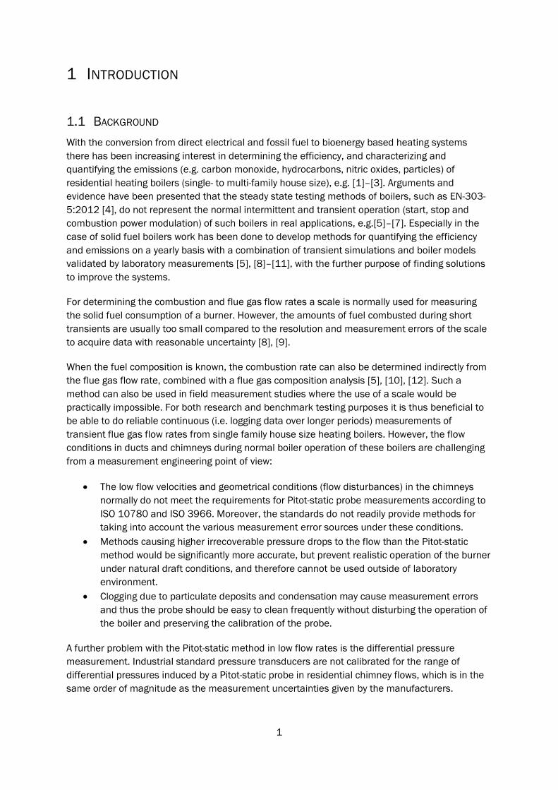
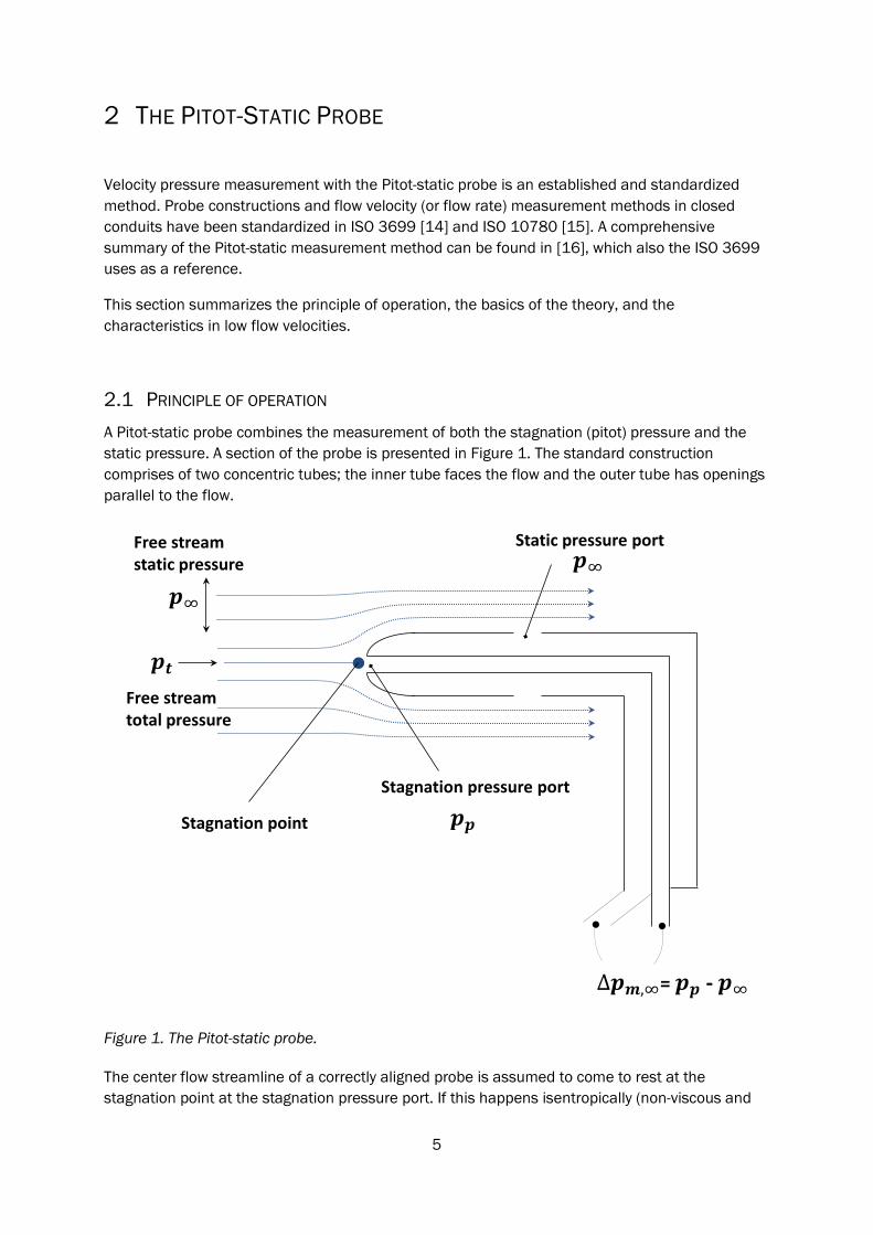
2.1 PRINCIPLE OF OPERATION A Pitot-static probe combines the measurement of both the stagnation (pitot) pressure and the static pressure. A section of the probe is presented in Figure 1. The standard construction comprises of two concentric tubes; the inner tube faces the flow and the outer tube has openings parallel to the flow.

Figure 1. The Pitot-static probe.

The center flow streamline of a correctly aligned probe is assumed to come to rest at the stagnation point at the stagnation pressure port. If this happens isentropically (non-viscous and

Stagnation pressure port

Static pressure port

= -

Free stream static pressure

Free stream total pressure

Stagnation point

6

incompressible fluid) the kinetic energy of the fluid is converted to pressure, namely velocity pressure. The total pressure (also called pitot pressure) at the stagnation point is thus the sum of the velocity pressure and the static pressure.

The streamlines of the fluid are parallel to the static pressure ports of a correctly aligned probe. Assuming a non-viscous fluid, no kinetic energy is converted to pressure and the openings are exposed only to the pressure perpendicular to the flow, i.e. the static pressure.

The gas volume of each tube is assumed to be at the same pressure as that of the fluid at the corresponding openings. The pressures of each volume can then be measured at the other end of the concentric tubes, either individually as 𝑝𝑝𝑝𝑝 and 𝑝𝑝∞, or as a differential pressure ∆𝑝𝑝𝑚𝑚,∞.

Various probe head shapes (e.g. ellipsoidal, hemispherical, cylindrical or tapered) have been developed and tested for different purposes and ISO 3699 gives recommendations for three types of heads.

In ISO 3699 the “stagnation pressure port” of Figure 1 is called “total pressure hole”, which can be misleading. With the conditions given in the standard the measured stagnation pressure is assumed to equal the total pressure. However, outside of the given 𝑅𝑅𝑅𝑅 and 𝑣𝑣 limits (see Table 2) this is not true, as will be described later. This report is considering flows below the given 𝑅𝑅𝑅𝑅 and 𝑣𝑣 limits and therefore the term “stagnation pressure port” is preferred to differentiate between the measured stagnation pressure and the (theoretical or true) total pressure.

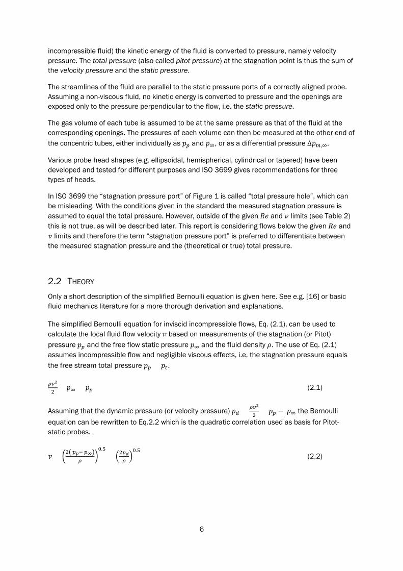
2.2 THEORY Only a short description of the simplified Bernoulli equation is given here. See e.g. [16] or basic fluid mechanics literature for a more thorough derivation and explanations.

The simplified Bernoulli equation for inviscid incompressible flows, Eq. (2.1), can be used to calculate the local fluid flow velocity 𝑣𝑣 based on measurements of the stagnation (or Pitot) pressure 𝑝𝑝𝑝𝑝 and the free flow static pressure 𝑝𝑝∞ and the fluid density 𝜌𝜌. The use of Eq. (2.1) assumes incompressible flow and negligible viscous effects, i.e. the stagnation pressure equals the free stream total pressure 𝑝𝑝𝑝𝑝 = 𝑝𝑝𝑡𝑡.

𝜌𝜌𝜌𝜌2

2+ 𝑝𝑝∞ = 𝑝𝑝𝑝𝑝 (2.1)

Assuming that the dynamic pressure (or velocity pressure) 𝑝𝑝𝑑𝑑 = 𝜌𝜌𝜌𝜌2

2= 𝑝𝑝𝑝𝑝 − 𝑝𝑝∞ the Bernoulli

equation can be rewritten to Eq.2.2 which is the quadratic correlation used as basis for Pitot-static probes.

𝑣𝑣 = �2� 𝑝𝑝𝑝𝑝− 𝑝𝑝∞�𝜌𝜌

�0.5

= �2𝑝𝑝𝑑𝑑𝜌𝜌�0.5

(2.2)

7

2.3 CALIBRATION For use with Pitot-static probes Eq. (2.2) is normally modified with an experimental calibration constant 𝐾𝐾 to correct the measured pressure difference ∆𝑝𝑝𝑚𝑚,∞ to the dynamic pressure 𝑝𝑝𝑑𝑑.

𝑣𝑣 ≈ 𝐾𝐾 �2∆𝑝𝑝𝑚𝑚,∞𝜌𝜌

�0.5

(2.3)

𝐾𝐾 is determined experimentally and for standard L-type Pitot-static probes 𝐾𝐾 ≈ 1.00 normally, when used within the requirements of the ISO 10780 or ISO 3966. It should be noted that 𝐾𝐾, as defined by ISO 10780, is linear and an average value for the calibration range, which must be within the requirements of the standard. Viscous effects with low flow rates thus cannot be taken into account for with this method and in such conditions the pressure coefficient presented in section 2.4 should be used instead.

2.4 CORRECTION FOR LOW RE – STAGNATION PRESSURE COEFFICIENT With low 𝑅𝑅𝑅𝑅 the assumption of inviscid and incompressible flow becomes gradually invalid resulting in that 𝑝𝑝𝑝𝑝 ≠ 𝑝𝑝𝑡𝑡. Correction factors for Pitot probes in low 𝑅𝑅𝑅𝑅𝑃𝑃𝑃𝑃𝑅𝑅 have been studied extensively, e.g. [17]–[20]. The characteristics of the stagnation pressure are normally studied and compared with the pressure coefficient 𝐶𝐶𝑝𝑝𝑝𝑝 defined by Eq. (2.4) describing the overestimation of the velocity pressure 𝑝𝑝𝑑𝑑 by the measured differential pressure ∆𝑝𝑝𝑚𝑚,∞.

𝐶𝐶𝑝𝑝𝑝𝑝 = 𝑝𝑝𝑝𝑝−𝑝𝑝∞12� 𝜌𝜌𝜌𝜌2

= ∆𝑝𝑝𝑚𝑚,∞𝑝𝑝𝑑𝑑

= 𝑓𝑓(𝑅𝑅𝑅𝑅𝑃𝑃𝑃𝑃𝑅𝑅) (2.4)

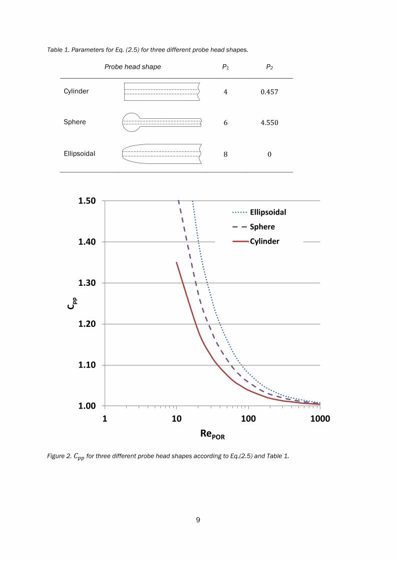
The correction for the viscous effects is shape dependent, and the various forms of the correction for different probe heads found in literature, e.g. [18], [21], [22], can be summarized with Eq. (2.5). The correction function approaches unity asymptotically with increasing 𝑅𝑅𝑅𝑅𝑃𝑃𝑃𝑃𝑅𝑅. 𝑃𝑃1 and 𝑃𝑃2 are shape dependent parameters and for some cases 𝑃𝑃2 = 0.

𝐶𝐶𝑝𝑝𝑝𝑝 = ∆𝑝𝑝𝑚𝑚,∞𝑝𝑝𝑑𝑑

= 1 + 𝑃𝑃1𝑅𝑅𝑅𝑅𝑃𝑃𝑃𝑃𝑃𝑃+𝑃𝑃2�𝑅𝑅𝑅𝑅𝑃𝑃𝑃𝑃𝑃𝑃

(2.5)

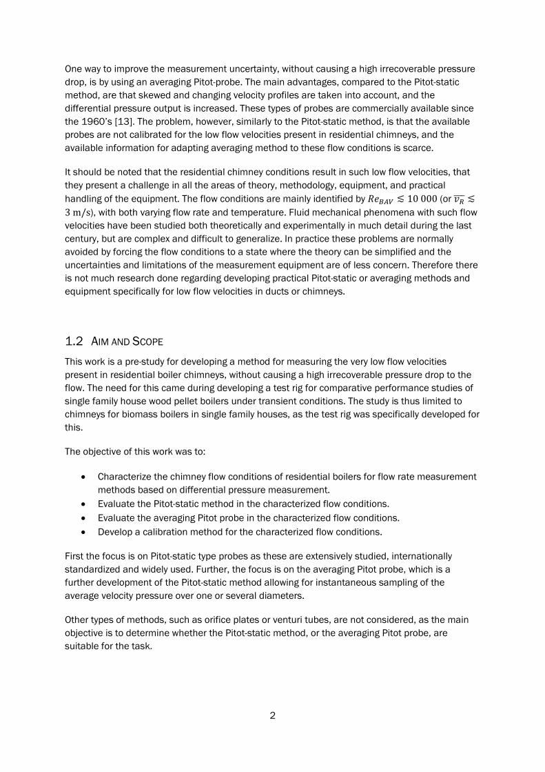
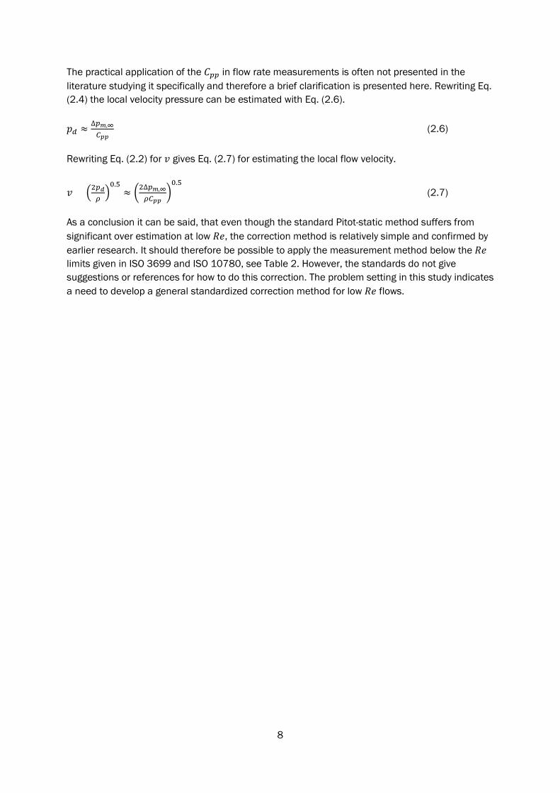
Example parameters for Eq. (2.5) for three different probe head shapes based on [21] are shown in Table 1 and the corresponding pressure coefficients in Figure 2. It can be seen that the correction quickly rises significantly for 𝑅𝑅𝑅𝑅𝑃𝑃𝑃𝑃𝑅𝑅 ≲ 150.

The pressure coefficients for different types of Pitot impact pressure probes are relatively constant for 𝑅𝑅𝑅𝑅𝑃𝑃𝑃𝑃𝑅𝑅 ≳ 500, as summarized in [21], but Pitot-static probes may suffer from changes already at higher 𝑅𝑅𝑅𝑅𝑃𝑃𝑃𝑃𝑅𝑅. The reported impact pressure coefficients slowly start to rise above unity already at 𝑅𝑅𝑅𝑅𝑃𝑃𝑃𝑃𝑅𝑅 ≈ 1000, but the really significant changes (over 2 % deviation) happen when 𝑅𝑅𝑅𝑅𝑃𝑃𝑃𝑃𝑅𝑅 ≲ 100.

The viscous effects are summarized and numerically studied more recently in [19] with the conclusion that the Bernoulli equation is prone to significant (over 2 %) error at 𝑅𝑅𝑅𝑅𝑃𝑃𝑃𝑃𝑅𝑅 < 45 and 𝑅𝑅𝑅𝑅𝑃𝑃𝑃𝑃𝑅𝑅 < 65 for hemispherical and blunt faced impact probe heads, respectively. These values are somewhat lower, but in agreement with the earlier mentioned 𝑅𝑅𝑅𝑅𝑃𝑃𝑃𝑃𝑅𝑅 ≲ 100 based on the summary in [21].

8

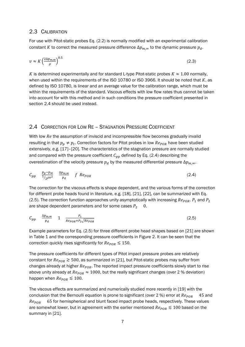
The practical application of the 𝐶𝐶𝑝𝑝𝑝𝑝 in flow rate measurements is often not presented in the literature studying it specifically and therefore a brief clarification is presented here. Rewriting Eq. (2.4) the local velocity pressure can be estimated with Eq. (2.6).

𝑝𝑝𝑑𝑑 ≈∆𝑝𝑝𝑚𝑚,∞𝐶𝐶𝑝𝑝𝑝𝑝

(2.6)

Rewriting Eq. (2.2) for 𝑣𝑣 gives Eq. (2.7) for estimating the local flow velocity.

𝑣𝑣 = �2𝑝𝑝𝑑𝑑𝜌𝜌�0.5

≈ �2∆𝑝𝑝𝑚𝑚,∞𝜌𝜌𝐶𝐶𝑝𝑝𝑝𝑝

�0.5

(2.7)

As a conclusion it can be said, that even though the standard Pitot-static method suffers from significant over estimation at low 𝑅𝑅𝑅𝑅, the correction method is relatively simple and confirmed by earlier research. It should therefore be possible to apply the measurement method below the 𝑅𝑅𝑅𝑅 limits given in ISO 3699 and ISO 10780, see Table 2. However, the standards do not give suggestions or references for how to do this correction. The problem setting in this study indicates a need to develop a general standardized correction method for low 𝑅𝑅𝑅𝑅 flows.

9

Table 1. Parameters for Eq. (2.5) for three different probe head shapes.

Probe head shape P1 P2

Cylinder

4 0.457

Sphere

6 4.550

Ellipsoidal

8 0

Figure 2. 𝐶𝐶𝑝𝑝𝑝𝑝 for three different probe head shapes according to Eq.(2.5) and Table 1.

1.00

1.10

1.20

1.30

1.40

1.50

1 10 100 1000

C pp

RePOR

Ellipsoidal

Sphere

Cylinder

10

3 THE PITOT-STATIC METHOD IN FLUE GAS FLOW RATE MEASUREMENTS

The ISO 10780 [15] and ISO 3966 [14] present standardized methods to determine the flow rate in a closed conduit using a Pitot-static probe. The average flow velocity of a cross section of the conduit is determined by traversing the Pitot-static probe through two or several diameters of the cross section. The measurement must be done during a steady state flow, i.e. the flow rate should not change significantly during the traversing.

The requirement of a steady state is obviously not possible to fulfill with processes for which the flow rate is changing faster than the traversing can be done. For continuous measurements of transient flue gas flows a single point velocity pressure measurement with a standard L-type (or S-type) Pitot-static probe is often done, assuming a certain velocity profile based on fluid mechanics or an initial traversing measurements [23], see section 4.3.4. This method is practically difficult to calibrate for the whole range of boiler operation as it would require long enough steady states at different combustion rates for the traversing measurements to be successful. Arbitrary steady states of sufficient durations are often prevented by both boiler system control algorithms and limitations of the heating load, which especially in field conditions often is the only available heat sink.

3.1 ISO 10780 AND ISO 3966 REQUIREMENTS AND LIMITATIONS

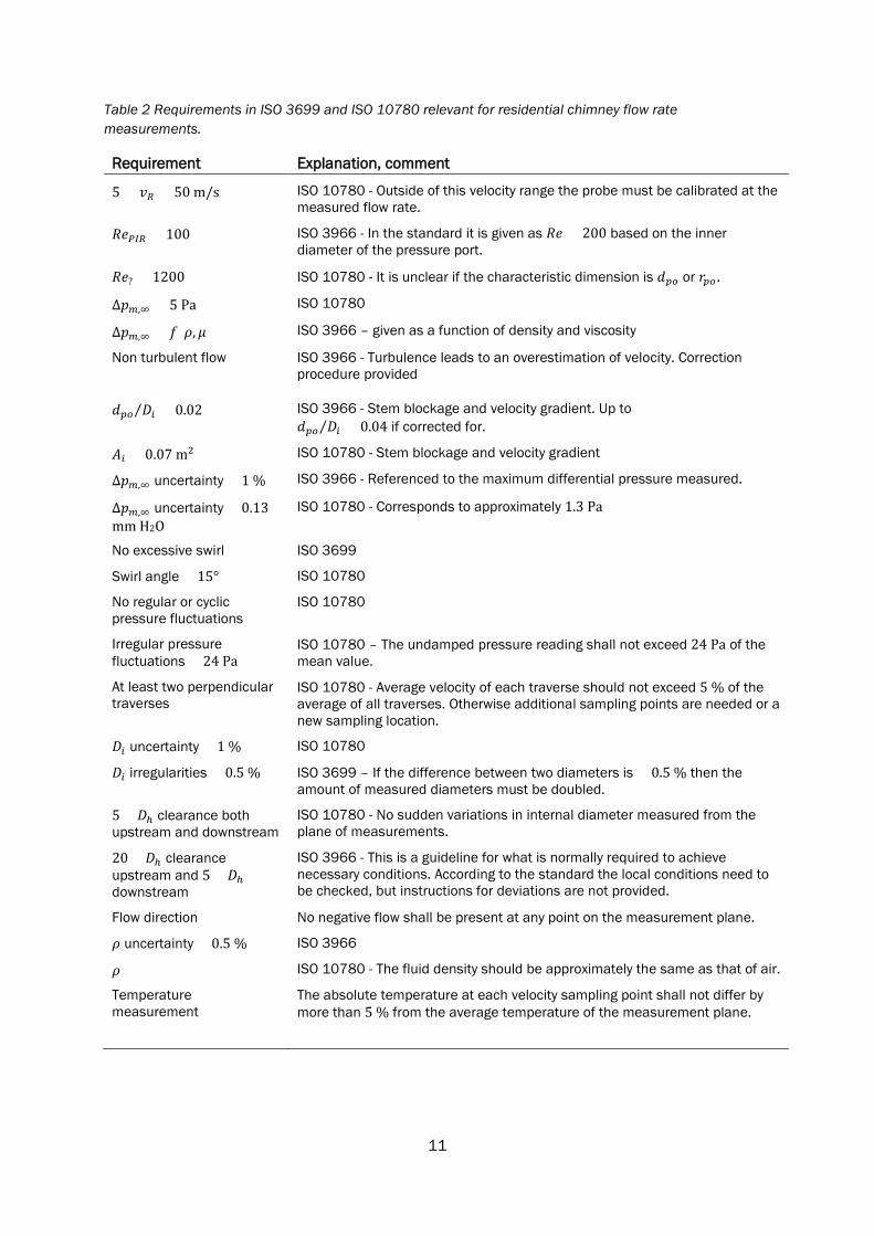
The ISO 10780 and ISO 3966 set a number of requirements on the Pitot-static method, mainly concerning the flow characteristics and geometry. The requirements relevant for SFH chimney flows are shown in Table 2. The requirements concerning high velocities are of no concern in residential chimneys, see Table 3.

Several of the assumptions (or requirements) regarding the use of the Pitot-static method in chimney flue gas flows become potentially invalid in some operational states of boilers, especially at low combustion rates. Robinson [24] summarizes the requirements set in ISO 10780 and ISO 3966, which are met questionably (or not met at all) in industrial chimney flows, arguing that a simple calibration coefficient is probably not sufficient to cover the wide range of operating conditions.

It should be pointed out that no standardized or recommended methods for correcting the measurement or estimating the uncertainty below the ISO 3966 and ISO 10780 requirements are readily provided by the standards and there are now easily applicable methods found in the literature.

11

Table 2 Requirements in ISO 3699 and ISO 10780 relevant for residential chimney flow rate measurements.

Requirement Explanation, comment

5 < 𝑣𝑣𝑅𝑅 < 50 m/s ISO 10780 - Outside of this velocity range the probe must be calibrated at the measured flow rate.

𝑅𝑅𝑅𝑅𝑃𝑃𝑃𝑃𝑅𝑅 > 100 ISO 3966 - In the standard it is given as 𝑅𝑅𝑅𝑅 > 200 based on the inner diameter of the pressure port.

𝑅𝑅𝑅𝑅? > 1200 ISO 10780 - It is unclear if the characteristic dimension is 𝑑𝑑𝑝𝑝𝑝𝑝 or 𝑟𝑟𝑝𝑝𝑝𝑝.

∆𝑝𝑝𝑚𝑚,∞ > 5 Pa ISO 10780

∆𝑝𝑝𝑚𝑚,∞ > 𝑓𝑓(𝜌𝜌, 𝜇𝜇) ISO 3966 – given as a function of density and viscosity

Non turbulent flow

ISO 3966 - Turbulence leads to an overestimation of velocity. Correction procedure provided

𝑑𝑑𝑝𝑝𝑝𝑝 𝐷𝐷𝑖𝑖⁄ < 0.02 ISO 3966 - Stem blockage and velocity gradient. Up to 𝑑𝑑𝑝𝑝𝑝𝑝 𝐷𝐷𝑖𝑖⁄ < 0.04 if corrected for.

𝐴𝐴𝑖𝑖 > 0.07 m2 ISO 10780 - Stem blockage and velocity gradient

∆𝑝𝑝𝑚𝑚,∞ uncertainty < 1 % ISO 3966 - Referenced to the maximum differential pressure measured.

∆𝑝𝑝𝑚𝑚,∞ uncertainty < 0.13 mm H2O

ISO 10780 - Corresponds to approximately 1.3 Pa

No excessive swirl ISO 3699

Swirl angle < 15° ISO 10780

No regular or cyclic pressure fluctuations

ISO 10780

Irregular pressure fluctuations < 24 Pa

ISO 10780 – The undamped pressure reading shall not exceed 24 Pa of the mean value.

At least two perpendicular traverses

ISO 10780 - Average velocity of each traverse should not exceed 5 % of the average of all traverses. Otherwise additional sampling points are needed or a new sampling location.

𝐷𝐷𝑖𝑖 uncertainty < 1 % ISO 10780

𝐷𝐷𝑖𝑖 irregularities < 0.5 % ISO 3699 – If the difference between two diameters is > 0.5 % then the amount of measured diameters must be doubled.

5 × 𝐷𝐷ℎ clearance both upstream and downstream

ISO 10780 - No sudden variations in internal diameter measured from the plane of measurements.

20 × 𝐷𝐷ℎ clearance upstream and 5 × 𝐷𝐷ℎ downstream

ISO 3966 - This is a guideline for what is normally required to achieve necessary conditions. According to the standard the local conditions need to be checked, but instructions for deviations are not provided.

Flow direction No negative flow shall be present at any point on the measurement plane.

𝜌𝜌 uncertainty < 0.5 % ISO 3966

𝜌𝜌 ISO 10780 - The fluid density should be approximately the same as that of air.

Temperature measurement

The absolute temperature at each velocity sampling point shall not differ by more than 5 % from the average temperature of the measurement plane.

12

3.2 LIMITATIONS IN THE DIFFERENTIAL PRESSURE MEASUREMENT A further complication regarding differential pressure based measurement methods at low flow velocities is the accuracy of the pressure measurement and the issue is briefly mentioned in [24]. A requirement in ISO 10780 is that the measured differential pressure must be greater than 5 Pa, which corresponds to approximately 3 m/s flow velocity, depending on the temperature (see e.g. Figure 15).

The differential pressures produced by Pitot-static probes in residential boiler chimney flue gas flows are in the order of a few Pa, mostly significantly under 5 Pa. Commercially available low differential pressure transducers are normally calibrated for a range of up to at least tens of Pa, e.g. 50 Pa or 100 Pa. This means that they are used below the lowest 10 % of their intended measurement range when used for chimney flow rate measurements with Pitot-static probes. Issues such as resolution, hysteresis and environmental error sources thus may become significant problems in the differential pressure measurement and should be evaluated.

Another requirement is the uncertainty level of the differential pressure measurement. In ISO 3699 a maximum of 1 % uncertainty referenced to the maximum differential pressure measured is allowed. In ISO 10780 an absolute level of up to ± 0.13 mm H2O, corresponding to ± 1.3Pa, is required. As an example, the national testing institute of Sweden (SP) can calibrate pressure points with an absolute uncertainty of ± 0.2 Pa. To fulfill the < 1 % uncertainty requirement the measured differential pressure would need to be at least 20 Pa with this calibration.

3.3 REPORTED ISSUES The Swedish Institute of Applied Environmental Research (ITM) does testing of accredited emissions monitoring organizations. ITM has reported the results of two tests where a number of organizations in field measurement conditions independently measured a flue gas flow from two industrial scale boilers (several MWth combustion power) with their preferred Pitot-static method (S or L probe) [25], [26]. The measurements are compared to a reference method showing that even when meeting the flow velocity requirements set in ISO 10780 [15] the results of the independent measurements varied ± 15 % from the reference flow rate. A similar test was done also in laboratory conditions with an impeller induced air flow (room temperature) at different flow velocities [27]. The results imply that even in controlled laboratory conditions, where all ISO 10780 requirements are met, ± 10 % deviations can be expected.

The UK National Physical Laboratory performed a questionnaire survey to the UK emissions monitoring community [24]. The results showed that a significant number of organizations were routinely performing measurements outside (namely below, because of low flow velocities) of the conditions given in ISO 10780, although the reference does not summarize how the organizations dealt with this.

The results of the survey on the UK measuring community imply that it is difficult to strictly apply the ISO standard methods for industrial scale boilers. The Swedish comparisons of independent Pitot-static measurements done in ideal measurement conditions imply uncertainties and repeatability which may not be satisfactory for benchmark testing and research purposes.

13

3.4 NEED FOR DEVELOPMENT OF METHODS FOR RESIDENTIAL BOILER CHIMNEY

CONDITIONS As a conclusion based on the above presented issues it can be said, that even though the Pitot-static method is a widely used and proven technique, in chimney flow conditions there is potential for relatively large measurement errors, which should either be calibrated for, or properly taken into account in the uncertainty analysis.

The survey and the tests presented in section 3.3 apply to industrial scale boilers. The flow velocities are normally lower for small residential boilers, based on which one could expect the problems similar, or more likely, worse. For residential boiler chimneys the flow conditions are probably always completely outside of the ISO 10780 [15] requirements, so the method and its stated uncertainties cannot be applied as such without an analysis of the conditions.

The ISO 10780 or ISO 3699, however, do not give methods or suggestions for how to perform measurements and analysis below the velocity or differential pressure limits given in the standard, which gives the objective for this study. A characterization of flow conditions in typical chimneys is needed so that a suitable measurement method can be chosen and developed.

14

4 CHIMNEY FLOW CHARACTERISTICS

4.1 RESIDENTIAL CHIMNEY BOUNDARY CONDITIONS In this section the typical conditions of residential boiler installations are presented, specifically regarding the flue gas flow in chimneys. It should be noted that strict boundaries are often difficult to define; there is a multitude of technical solutions for boilers and burners with corresponding manufacturer specifications, the systems are often retrofitted and therefore adapted to existing chimneys, different requirements of laboratory testing result in different test methods and rigs, etc. It should therefore be kept in mind that the conditions and boundaries given here are not strict, but are helpful as a reference point for analysis and discussion.

4.1.1 TYPICAL BOILER INSTALLATIONS

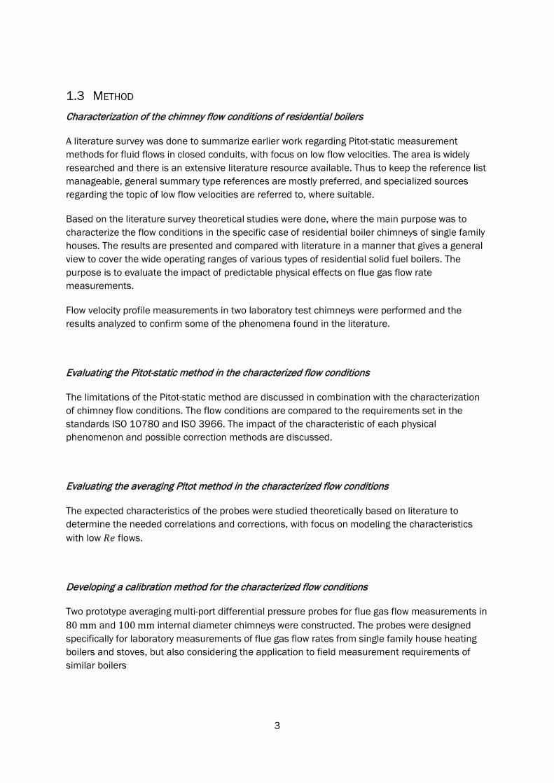
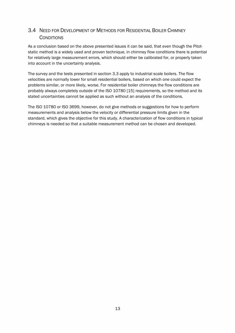
Figure 3 shows a simplified illustration of a solid fuel boiler or stove installed in a residential building. A boiler is typically situated in a boiler room and a stove e.g. in a living room.

Normally no measurements are done, other than necessary variables for the control functions and alarms. The user keeps track on system performance by functionality, fuel consumption and required maintenance work.

The flue gas exhaust of the boiler/stove is connected to a chimney. The chimney is often a brick construction and in the Nordic countries it is normally fitted with an inner tube of e.g. stainless steel, when an oil or pellet boiler is used.

The burner has a combustion air fan, but normally no flue gas fan is used if the draft induced by the chimney is sufficient, see section 4.1.3. The burner also may be integrated in the boiler or stove construction, which is most often the case with stoves.

Normally no flue gas cleaning systems (e.g. filters, cyclones, scrubbers) are installed. Currently there are no requirements for flue gas cleaning as the emissions are controlled by requirements on the boiler and burner performance instead.

Water mantled boilers/stoves are connected to the heating and domestic hot water production of the house, which are the heat load. Stoves are often without a water mantle, i.e. heat is transferred directly to the ambient via radiation and convection.

15

Figure 3. Illustration of a boiler or stove installed in a detached house.

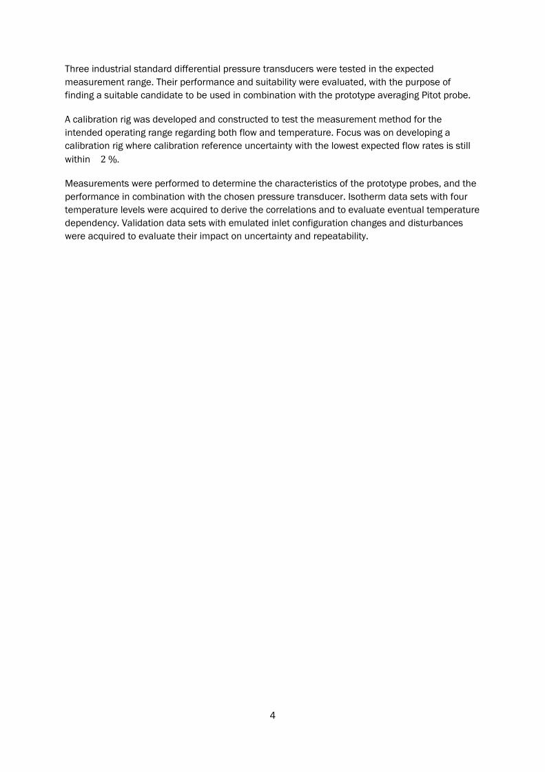
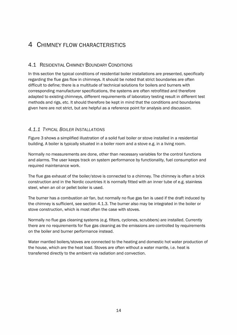
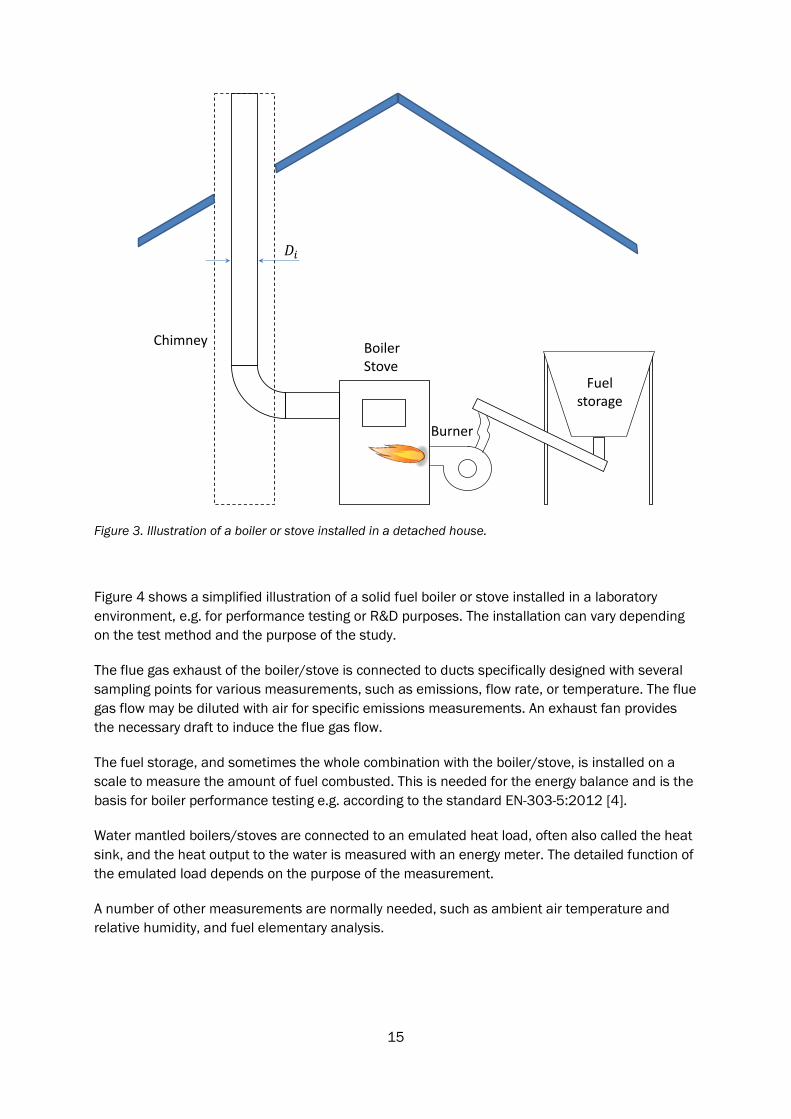
Figure 4 shows a simplified illustration of a solid fuel boiler or stove installed in a laboratory environment, e.g. for performance testing or R&D purposes. The installation can vary depending on the test method and the purpose of the study.

The flue gas exhaust of the boiler/stove is connected to ducts specifically designed with several sampling points for various measurements, such as emissions, flow rate, or temperature. The flue gas flow may be diluted with air for specific emissions measurements. An exhaust fan provides the necessary draft to induce the flue gas flow.

The fuel storage, and sometimes the whole combination with the boiler/stove, is installed on a scale to measure the amount of fuel combusted. This is needed for the energy balance and is the basis for boiler performance testing e.g. according to the standard EN-303-5:2012 [4].

Water mantled boilers/stoves are connected to an emulated heat load, often also called the heat sink, and the heat output to the water is measured with an energy meter. The detailed function of the emulated load depends on the purpose of the measurement.

A number of other measurements are normally needed, such as ambient air temperature and relative humidity, and fuel elementary analysis.

BoilerStove

Chimney

Burner

Fuel storage

16

Figure 4. Illustration of a boiler or stove connected to ducts in a laboratory environment.

4.1.2 PHYSICAL AND COMBUSTION DATA FOR RESIDENTIAL BOILER OPERATION

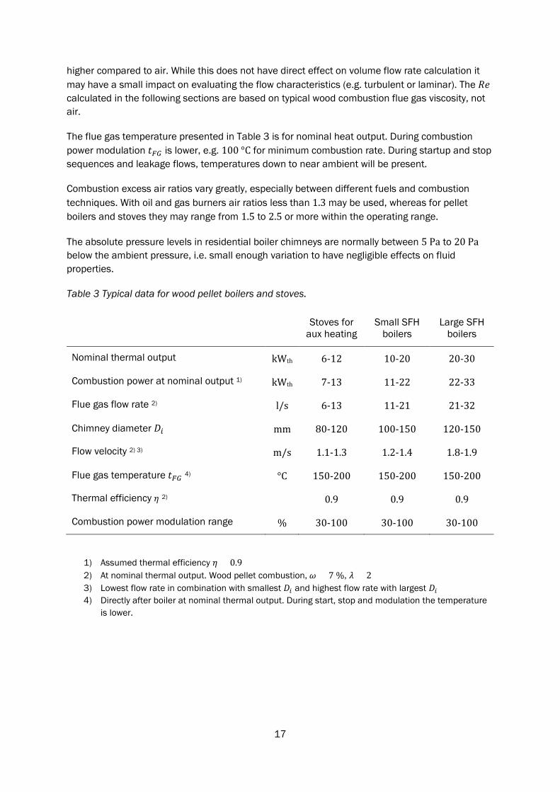
Key data for typical operating conditions of residential boilers are shown in table 3. Note that there is no generally standardized classification (stoves, small, large) of boilers. Table 3 thus represents what is a normally considered classification in the Nordic Countries and used in the discussions of this study.

The theoretical 𝑅𝑅𝑅𝑅𝐵𝐵𝐵𝐵𝐵𝐵 of flue gas flows in chimneys vary mostly dependent on fuel composition, combustion power and burner excess air setting (the three together defining the flue gas flow rate), chimney internal diameter, and the temperature of the flue gas entering the chimney.

The used fuel is normally wood (logs, chips or pellets), oil or gas. Other fuels are also used, e.g. the use of field crops pressed to pellets may be used, although not common. Flue gas from wood combustion is assumed throughout this study, although the properties of the other flue gases from other fuels mentioned are close enough for the conclusions to be generalized in most cases.

The kinematic viscosity of flue gas 50 °C < 𝑡𝑡𝐹𝐹𝐹𝐹 < 200 °C (from biomass combustion) is approximately 10 % to 15 % lower compared to air, and since it is the divider in Eq. (4.1) the effect is similar also on 𝑅𝑅𝑅𝑅, inversely, so that the 𝑅𝑅𝑅𝑅 in this temperature range are 10 % to 15 %

BoilerStove

Exhaust fan

Burner

Scale

DilutionEmissionsFlow rateTemperature

Fuel storage

Sampling for:

17

higher compared to air. While this does not have direct effect on volume flow rate calculation it may have a small impact on evaluating the flow characteristics (e.g. turbulent or laminar). The 𝑅𝑅𝑅𝑅 calculated in the following sections are based on typical wood combustion flue gas viscosity, not air.

The flue gas temperature presented in Table 3 is for nominal heat output. During combustion power modulation 𝑡𝑡𝐹𝐹𝐹𝐹 is lower, e.g. 100 °C for minimum combustion rate. During startup and stop sequences and leakage flows, temperatures down to near ambient will be present.

Combustion excess air ratios vary greatly, especially between different fuels and combustion techniques. With oil and gas burners air ratios less than 1.3 may be used, whereas for pellet boilers and stoves they may range from 1.5 to 2.5 or more within the operating range.

The absolute pressure levels in residential boiler chimneys are normally between 5 Pa to 20 Pa below the ambient pressure, i.e. small enough variation to have negligible effects on fluid properties.

Table 3 Typical data for wood pellet boilers and stoves.

Stoves for aux heating

Small SFH boilers

Large SFH boilers

Nominal thermal output kWth 6-12 10-20 20-30

Combustion power at nominal output 1) kWth 7-13 11-22 22-33

Flue gas flow rate 2) l/s 6-13 11-21 21-32

Chimney diameter 𝐷𝐷𝑖𝑖 mm 80-120 100-150 120-150

Flow velocity 2) 3) m/s 1.1-1.3 1.2-1.4 1.8-1.9

Flue gas temperature 𝑡𝑡𝐹𝐹𝐹𝐹 4) °C 150-200 150-200 150-200

Thermal efficiency 𝜂𝜂 2) 0.9 0.9 0.9

Combustion power modulation range % 30-100 30-100 30-100

1) Assumed thermal efficiency 𝜂𝜂 = 0.9 2) At nominal thermal output. Wood pellet combustion, 𝜔𝜔 = 7 %, 𝜆𝜆 = 2 3) Lowest flow rate in combination with smallest 𝐷𝐷𝑖𝑖 and highest flow rate with largest 𝐷𝐷𝑖𝑖 4) Directly after boiler at nominal thermal output. During start, stop and modulation the temperature

is lower.

18

4.1.3 CHIMNEY DIAMETERS

Chimney internal diameters 𝐷𝐷𝑖𝑖 vary and there are no strict rules for sizing. Chimney sizing depends on manufacturer recommendations and available height, with the goal of achieving an appropriate draft for the burner to function well. The 𝐷𝐷𝑖𝑖 presented in Table 3 are typical recommended values from wood pellet boiler and stove manufacturers.

The draft in such chimneys is usually in the order of -8 Pa to -15 Pa relative to ambient pressure, measured in the boiler combustion chamber. This sets limits to the irrecoverable pressure drop that additional disturbances, e.g. a measurement probe, can cause to the flue gas flow without significantly disturbing the operation of the burner, or causing flue gas to leak into the room where the boiler is situated. This limit of maximum irrecoverable pressure drop is difficult to quantify, as it depends on the burner, boiler, chimney sizing, and local conditions.

Pellet boilers and stoves are often retrofitted to an existing chimney of a specific dimension, which originally may have been serving an oil boiler or a wood log boiler/stove. The chimney can then be left without changes if the configuration works without problems, or fitted with an internal pipe of appropriate 𝐷𝐷𝑖𝑖 to improve the performance or to overcome problems (e.g. too strong draft or water vapor condensation). A flue gas fan needs to be fitted in the chimney if a sufficient 𝐷𝐷𝑖𝑖 for is not possible.

If the boiler is designed also for wood log combustion, in addition to a wood pellet burner, then 𝐷𝐷𝑖𝑖 = 150 mm is normally recommended. This is because of the higher momentary combustion power and flue gas flow of the wood log combustion process.

The laboratory chimney diameters chosen in this work were 𝐷𝐷𝑖𝑖 = 80 mm to 𝐷𝐷𝑖𝑖 = 100 mm, see section 6. These two values are used as examples throughout the study and will be referred to as D80 and D100.

The chosen 𝐷𝐷𝑖𝑖 for the test chimneys are in the lowest range compared to chimneys used in real conditions, in order to increase the flow velocity, i.e. increase the signal output and thus the accuracy of the flow rate measurement. It should therefore be kept in mind that the figures and conclusions presented in this work are somewhat optimistic for real field conditions, where 120 mm < 𝐷𝐷𝑖𝑖 < 150 mm chimneys are more common for boilers and 100 mm < 𝐷𝐷𝑖𝑖 < 120 mm for stoves. For comparison, the flue gas flow velocity (and measured velocity pressure) is roughly halved if the 𝐷𝐷𝑖𝑖 is increased from 100 mm to 150 mm.

19

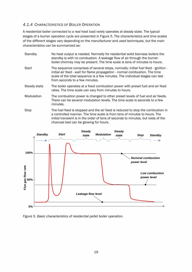
4.1.4 CHARACTERISTICS OF BOILER OPERATION

A residential boiler connected to a real heat load rarely operates at steady state. The typical stages of a burner operation cycle are presented in Figure 5. The characteristics and time scales of the different stages vary depending on the manufacturer and used techniques, but the main characteristics can be summarized as:

Standby No heat output is needed. Normally for residential solid biomass boilers the standby is with no combustion. A leakage flow of air through the burner-boiler-chimney may be present. The time scale is tens of minutes to hours.

Start The sequence comprises of several steps, normally: initial fuel feed - ignition - initial air feed - wait for flame propagation - normal combustion. The time scale of the total sequence is a few minutes. The individual stages can last from seconds to a few minutes.

Steady state The boiler operates at a fixed combustion power with preset fuel and air feed rates. The time scale can vary from minutes to hours.

Modulation The combustion power is changed to other preset levels of fuel and air feeds. There can be several modulation levels. The time scale is seconds to a few minutes.

Stop The fuel feed is stopped and the air feed is reduced to stop the combustion in a controlled manner. The time scale is from tens of minutes to hours. The initial transient is in the order of tens of seconds to minutes, but rests of the charcoal bed can be glowing for hours.

Figure 5. Basic characteristics of residential pellet boiler operation.

--

--

--

100%

50%

0%

Flue

gas

flow

rate

Nominal combustion power level

Leakage flow level

Start StopSteady state

Low combustion power level

ModulationSteady stateStandby Standby

20

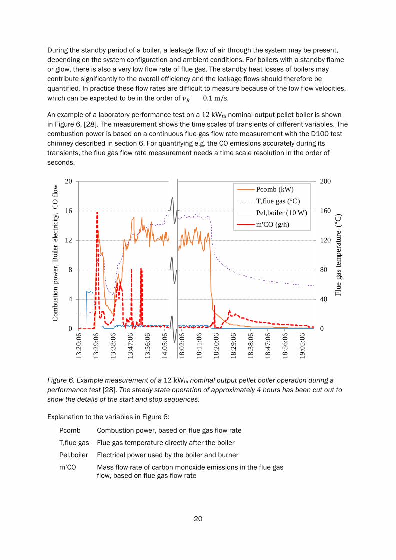
During the standby period of a boiler, a leakage flow of air through the system may be present, depending on the system configuration and ambient conditions. For boilers with a standby flame or glow, there is also a very low flow rate of flue gas. The standby heat losses of boilers may contribute significantly to the overall efficiency and the leakage flows should therefore be quantified. In practice these flow rates are difficult to measure because of the low flow velocities, which can be expected to be in the order of 𝑣𝑣𝑅𝑅��� < 0.1 m/s.

An example of a laboratory performance test on a 12 kWth nominal output pellet boiler is shown in Figure 6, [28]. The measurement shows the time scales of transients of different variables. The combustion power is based on a continuous flue gas flow rate measurement with the D100 test chimney described in section 6. For quantifying e.g. the CO emissions accurately during its transients, the flue gas flow rate measurement needs a time scale resolution in the order of seconds.

Figure 6. Example measurement of a 12 kWth nominal output pellet boiler operation during a performance test [28]. The steady state operation of approximately 4 hours has been cut out to show the details of the start and stop sequences.

Explanation to the variables in Figure 6:

Pcomb Combustion power, based on flue gas flow rate

T,flue gas Flue gas temperature directly after the boiler

Pel,boiler Electrical power used by the boiler and burner

m’CO Mass flow rate of carbon monoxide emissions in the flue gas flow, based on flue gas flow rate

0

40

80

120

160

200

0

4

8

12

16

20

13:2

0:06

13:2

9:06

13:3

8:06

13:4

7:06

13:5

6:06

14:0

5:06

18:0

2:06

18:1

1:06

18:2

0:06

18:2

9:06

18:3

8:06

18:4

7:06

18:5

6:06

19:0

5:06

Flue

gas

tem

pera

ture

(°C

)

Com

bust

ion

pow

er, B

oile

r el

ectri

city

, C

O fl

ow Pcomb (kW)T,flue gas (°C)Pel,boiler (10 W)m'CO (g/h)

21

4.2 BULK AVERAGE REYNOLDS NUMBER AND FLOW TYPE

4.2.1 THE REYNOLDS NUMBER Flow characteristics relevant to flow measurement methods are usually related to the dimensionless Reynolds number 𝑅𝑅𝑅𝑅, Eq. (4.1).

𝑅𝑅𝑅𝑅 = 𝜌𝜌𝑙𝑙𝐻𝐻𝜈𝜈

(4.1)

𝑅𝑅𝑅𝑅 is referenced to a characteristic (or hydraulic) length 𝑙𝑙𝐻𝐻, which in the case of pipes and cylinders is often the internal or external diameter. It should be noted that when discussing flow characteristics and flow measurements the 𝑅𝑅𝑅𝑅 can be defined in different ways:

For internal flows in e.g. ducts, 𝑅𝑅𝑅𝑅 is usually based on the average bulk flow velocity in the duct and the internal hydraulic diameter of the duct.

For an in-flow probe, e.g. a Pitot-static probe, in research results 𝑅𝑅𝑅𝑅 is usually based on its (outer) hydraulic radius and the local flow velocity, although the outer diameter is sometimes used.

For Pitot probes also a 𝑅𝑅𝑅𝑅 based on the probe impact pressure port diameter is used to check for possible viscous damping effects in the internal tube passages. In the available literature also the diameter is sometimes used.

For cylinders in cross flows 𝑅𝑅𝑅𝑅 is normally based on the outer diameter.

Other characteristic measures are also used, e.g. diameters or lengths instead of radii.

These definitions can easily cause confusion as the definition depends on the subject discussed, which can change even within the same sentence. Also adding to the difficulty of interpreting literature is mixing the use of radii with the engineering praxis of using diameters when e.g. pipe and bore hole dimensions are discussed. Already in the earliest work a misinterpretation of inner and outer diameters is pointed out as a reason for wrong conclusions [17]. Therefore, unless otherwise mentioned, the following subscripts will be used to differentiate the probe related external and internal 𝑅𝑅𝑅𝑅 from the duct bulk flow 𝑅𝑅𝑅𝑅:

BAV – Bulk Average Velocity – 𝑅𝑅𝑅𝑅𝐵𝐵𝐵𝐵𝐵𝐵 is based on the duct internal hydraulic diameter and average bulk flow velocity.

POR – Probe Outer Radius – 𝑅𝑅𝑅𝑅𝑃𝑃𝑃𝑃𝑅𝑅 is based on the probe outer radius and local flow velocity. Normally used for Pitot (static) probes.

PIR – Probe Internal Radius – 𝑅𝑅𝑅𝑅𝑃𝑃𝑃𝑃𝑅𝑅 is based on the impact pressure port radius and local flow velocity. Normally used for Pitot (static) probes. Note that ISO 3966 uses diameter, which deviates from praxis in literature.

POD – Probe Outer Diameter – 𝑅𝑅𝑅𝑅𝑃𝑃𝑃𝑃𝑃𝑃 is based on the outer probe diameter and local flow velocity. Specifically used for cylinders in cross flow. See section 5.2 for more detailed explanation.

22

4.2.2 CRITICAL REYNOLDS NUMBER AND TRANSITION OF FLOW TYPE

Starting with a laminar flow type, gradually increasing the flow rate the flow becomes unstable (labile) when the 𝑅𝑅𝑅𝑅𝐵𝐵𝐵𝐵𝐵𝐵 is greater than the critical Reynolds number 𝑅𝑅𝑅𝑅𝑐𝑐𝑐𝑐𝑖𝑖𝑡𝑡. An experimentally shown and generally accepted limit is 𝑅𝑅𝑅𝑅𝑐𝑐𝑐𝑐𝑖𝑖𝑡𝑡 = 2300, although a value of 𝑅𝑅𝑅𝑅𝑐𝑐𝑐𝑐𝑖𝑖𝑡𝑡 = 2000 is also sometimes used, e.g. [16], [29]–[31]. 𝑅𝑅𝑅𝑅𝑐𝑐𝑐𝑐𝑖𝑖𝑡𝑡 is actually not a fixed value, and depends on the upstream flow conditions, inlet configuration, pipe internal surface roughness, and whether the flow rate is increasing or decreasing [30], [31].

While it is reported that under special conditions laminar flows can occur far beyond 𝑅𝑅𝑅𝑅𝐵𝐵𝐵𝐵𝐵𝐵 >2300, there is a somewhat stricter lower limit of 𝑅𝑅𝑅𝑅𝑐𝑐𝑐𝑐𝑖𝑖𝑡𝑡 ≈ 2000, below which the flow can be said almost always to be laminar even with strong disturbances in the flow, because of predominant viscous forces quickly damping any disturbances [30], [31].

When 𝑅𝑅𝑅𝑅𝐵𝐵𝐵𝐵𝐵𝐵 > 𝑅𝑅𝑅𝑅𝑐𝑐𝑐𝑐𝑖𝑖𝑡𝑡 it indicates that even a small disturbance can change the flow from laminar to turbulent and thus a similar more fixed limit as the 𝑅𝑅𝑅𝑅𝑐𝑐𝑐𝑐𝑖𝑖𝑡𝑡 ≈ 2000 cannot be generalized for when the flow always could be said to be turbulent, as it is dependent on the various factors mentioned. Different values can be found in literature, ranging 3000 ≲ 𝑅𝑅𝑅𝑅𝑐𝑐𝑐𝑐𝑖𝑖𝑡𝑡 ≲ 10000, [29], [30], [32], [33], although these are usually laboratory results for smooth pipes with careful initial conditioning. For most practical engineering applications 2000 ≲ 𝑅𝑅𝑅𝑅𝑐𝑐𝑐𝑐𝑖𝑖𝑡𝑡 ≲ 4000 can be assumed [30]. This range, where the transition from laminar to turbulent flow is most likely to happen, is generally referred to as the transition regime (or e.g. transition zone, critical regime).

4.2.3 REYNOLDS NUMBERS AND FLOW TYPES IN RESIDENTIAL CHIMNEYS

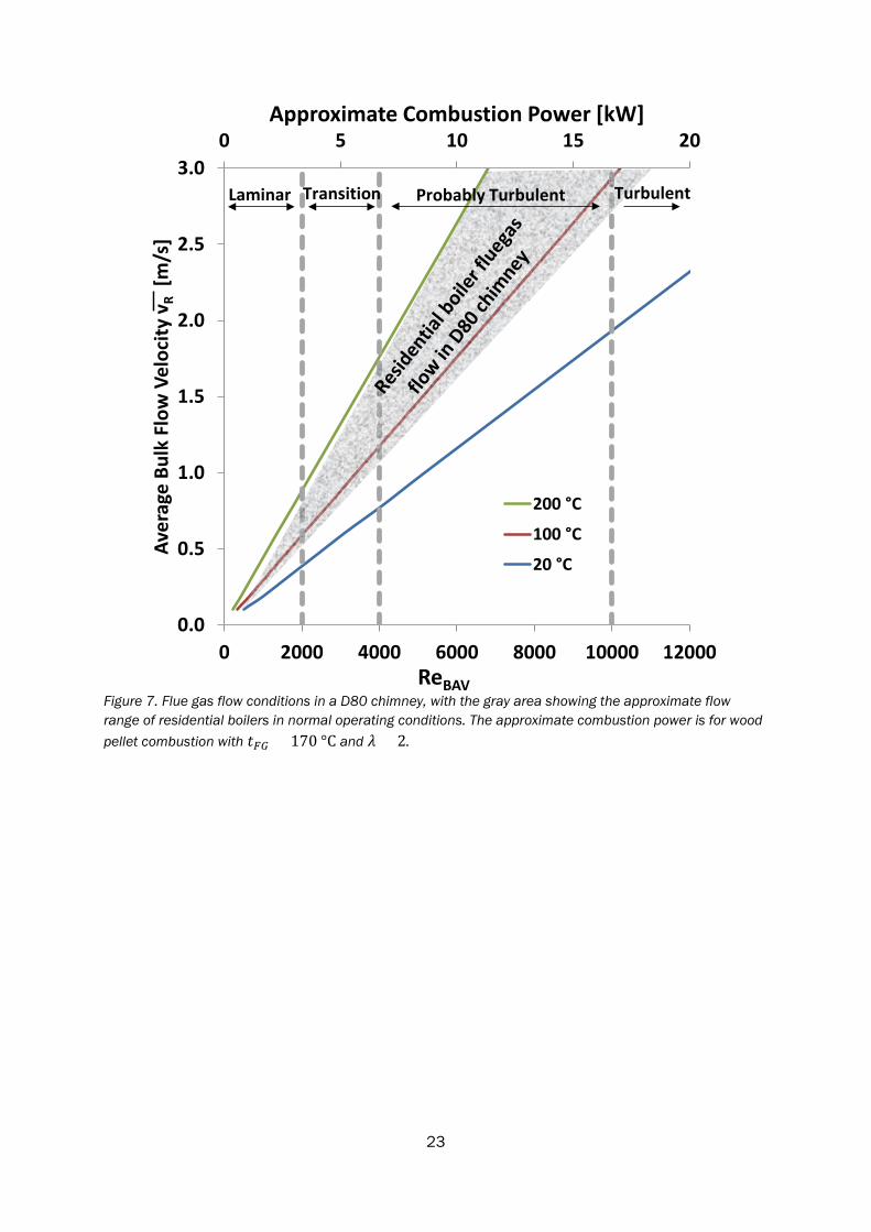
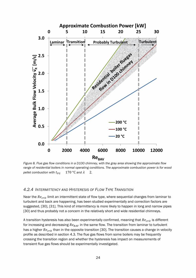
The flow characteristics of flue gas flows from wood pellet combustion in D80 and D100 chimneys are summarized in Figures 7 and 8.

The gray area shows approximately the flow range when the combustion rate is modulated from startup (which can be close to zero air leakage flow rate at room temperature) to full nominal combustion power (flue gas at around 100 °C to 200 °C). Boilers and burners of different types end up in various operational states depending on the combustion technique, fuel properties and burner settings, and thus the gray area also covers a wide range of temperatures and excess air ratios.

The values 𝑅𝑅𝑅𝑅𝑐𝑐𝑐𝑐𝑖𝑖𝑡𝑡 = 2000, 𝑅𝑅𝑅𝑅𝑐𝑐𝑐𝑐𝑖𝑖𝑡𝑡 = 4000 and 𝑅𝑅𝑅𝑅𝑐𝑐𝑐𝑐𝑖𝑖𝑡𝑡 = 10000 are also shown for giving an estimation of the flow characteristic, keeping in mind that for 𝑅𝑅𝑅𝑅𝐵𝐵𝐵𝐵𝐵𝐵 > 4000 the flow type is most likely turbulent in chimney conditions. It can be seen that the normal flue gas flow characteristics for these boilers range from laminar, over the transition regime, reaching into a regime, where one can be relatively certain of a fully developed turbulent flow, meaning that a measurement method need to take into account all these characteristics.

The results show that the calculated average flow velocities are consistently below the 5 m/s to 50 m/s validity range given in ISO 10780 [15]. It should be noted that in practice chimneys have larger diameters, i.e. lower flow velocities, than the chosen D80 and D100, see section 4.1.2.

23

Figure 7. Flue gas flow conditions in a D80 chimney, with the gray area showing the approximate flow range of residential boilers in normal operating conditions. The approximate combustion power is for wood pellet combustion with 𝑡𝑡𝐹𝐹𝐹𝐹 = 170 °C and 𝜆𝜆 = 2.

0 5 10 15 20

0.0

0.5

1.0

1.5

2.0

2.5

3.0

0 2000 4000 6000 8000 10000 12000

Approximate Combustion Power [kW]

Aver

age

Bulk

Flo

w V

eloc

ity v

R[m

/s]

ReBAV

200 °C

100 °C

20 °C

TransitionLaminar TurbulentProbably Turbulent

24

Figure 8. Flue gas flow conditions in a D100 chimney, with the gray area showing the approximate flow range of residential boilers in normal operating conditions. The approximate combustion power is for wood pellet combustion with 𝑡𝑡𝐹𝐹𝐹𝐹 = 170 °C and 𝜆𝜆 = 2.

4.2.4 INTERMITTENCY AND HYSTERESIS OF FLOW TYPE TRANSITION

Near the 𝑅𝑅𝑅𝑅𝑐𝑐𝑐𝑐𝑖𝑖𝑡𝑡 limit an intermittent state of flow type, where sequential changes from laminar to turbulent and back are happening, has been studied experimentally and correction factors are suggested, [30], [31]. This kind of intermittency is more likely to happen in long and narrow pipes [30] and thus probably not a concern in the relatively short and wide residential chimneys.

A transition hysteresis has also been experimentally confirmed, meaning that 𝑅𝑅𝑅𝑅𝑐𝑐𝑐𝑐𝑖𝑖𝑡𝑡 is different for increasing and decreasing 𝑅𝑅𝑅𝑅𝐵𝐵𝐵𝐵𝐵𝐵 in the same flow. The transition from laminar to turbulent has a higher 𝑅𝑅𝑅𝑅𝑐𝑐𝑐𝑐𝑖𝑖𝑡𝑡 than in the opposite transition [30]. The transition causes a change in velocity profile as described in section 4.3. The flue gas flows from some boilers may be frequently crossing the transition region and whether the hysteresis has impact on measurements of transient flue gas flows should be experimentally investigated.

0 5 10 15 20 25 30

0.0

0.5

1.0

1.5

2.0

2.5

3.0

0 2000 4000 6000 8000 10000 12000

Approximate Combustion Power [kW]Av

erag

e Bu

lk F

low

Vel

ocity

vR

[m/s

]

ReBAV

200 °C

100 °C

20 °C

TransitionLaminar TurbulentProbably Turbulent

25

4.3 FLOW VELOCITY PROFILES

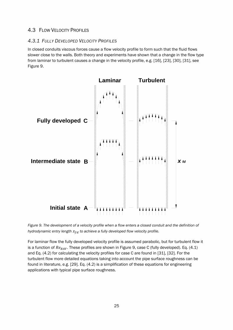
4.3.1 FULLY DEVELOPED VELOCITY PROFILES In closed conduits viscous forces cause a flow velocity profile to form such that the fluid flows slower close to the walls. Both theory and experiments have shown that a change in the flow type from laminar to turbulent causes a change in the velocity profile, e.g. [16], [23], [30], [31], see Figure 9.

Figure 9. The development of a velocity profile when a flow enters a closed conduit and the definition of hydrodynamic entry length 𝑥𝑥𝑓𝑓𝑑𝑑 to achieve a fully developed flow velocity profile.

For laminar flow the fully developed velocity profile is assumed parabolic, but for turbulent flow it is a function of 𝑅𝑅𝑅𝑅𝐵𝐵𝐵𝐵𝐵𝐵. These profiles are shown in Figure 9, case C (fully developed). Eq. (4.1) and Eq. (4.2) for calculating the velocity profiles for case C are found in [31], [32]. For the turbulent flow more detailed equations taking into account the pipe surface roughness can be found in literature, e.g. [29]. Eq. (4.2) is a simplification of these equations for engineering applications with typical pipe surface roughness.

x fd

TurbulentLaminar

Fully developed

Initial state

Intermediate state

A

B

C

26

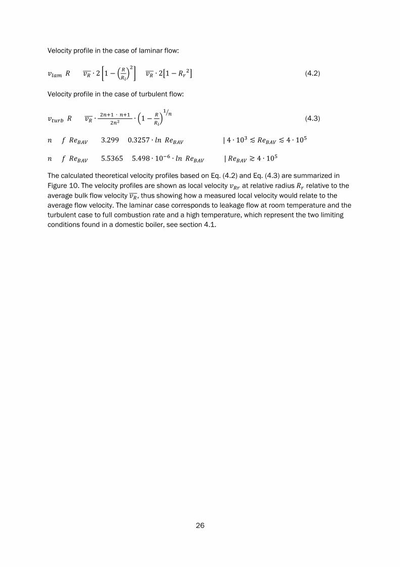
Velocity profile in the case of laminar flow:

𝑣𝑣𝑙𝑙𝑙𝑙𝑚𝑚(𝑅𝑅) = 𝑣𝑣𝑅𝑅��� ∙ 2 �1 − �𝑅𝑅𝑅𝑅𝑖𝑖�2� = 𝑣𝑣𝑅𝑅��� ∙ 2�1 − 𝑅𝑅𝑐𝑐2� (4.2)

Velocity profile in the case of turbulent flow:

𝑣𝑣𝑡𝑡𝑡𝑡𝑐𝑐𝑡𝑡(𝑅𝑅) = 𝑣𝑣𝑅𝑅��� ∙(2𝑛𝑛+1)∙(𝑛𝑛+1)

2𝑛𝑛2∙ �1 − 𝑅𝑅

𝑅𝑅𝑖𝑖�1 𝑛𝑛�

(4.3)

𝑛𝑛 = 𝑓𝑓(𝑅𝑅𝑅𝑅𝐵𝐵𝐵𝐵𝐵𝐵) = 3.299 + 0.3257 ∙ 𝑙𝑙𝑛𝑛(𝑅𝑅𝑅𝑅𝐵𝐵𝐵𝐵𝐵𝐵) | 4 ∙ 103 ≲ 𝑅𝑅𝑅𝑅𝐵𝐵𝐵𝐵𝐵𝐵 ≲ 4 ∙ 105

𝑛𝑛 = 𝑓𝑓(𝑅𝑅𝑅𝑅𝐵𝐵𝐵𝐵𝐵𝐵) = 5.5365 + 5.498 ∙ 10−6 ∙ 𝑙𝑙𝑛𝑛(𝑅𝑅𝑅𝑅𝐵𝐵𝐵𝐵𝐵𝐵) | 𝑅𝑅𝑅𝑅𝐵𝐵𝐵𝐵𝐵𝐵 ≳ 4 ∙ 105

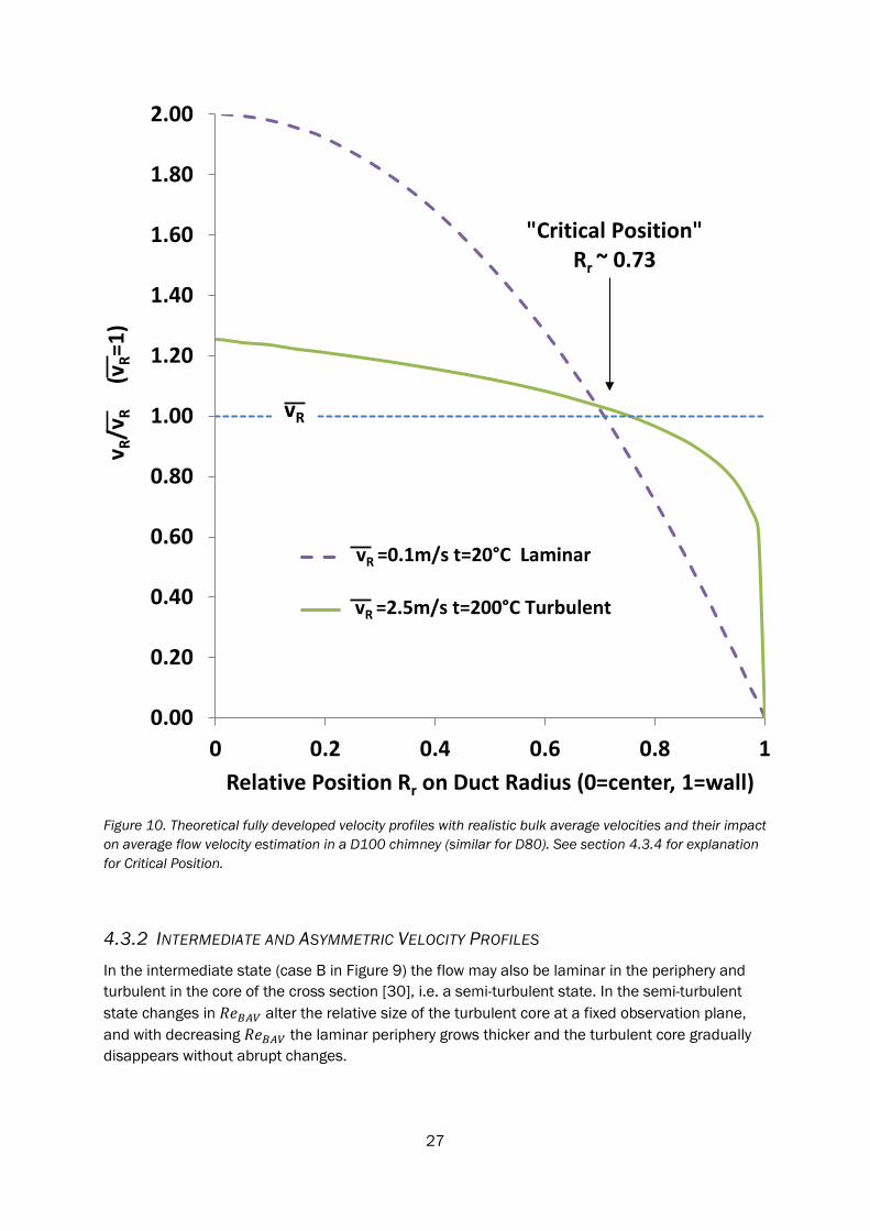
The calculated theoretical velocity profiles based on Eq. (4.2) and Eq. (4.3) are summarized in Figure 10. The velocity profiles are shown as local velocity 𝑣𝑣𝑅𝑅𝑐𝑐 at relative radius 𝑅𝑅𝑐𝑐 relative to the average bulk flow velocity 𝑣𝑣𝑅𝑅���, thus showing how a measured local velocity would relate to the average flow velocity. The laminar case corresponds to leakage flow at room temperature and the turbulent case to full combustion rate and a high temperature, which represent the two limiting conditions found in a domestic boiler, see section 4.1.

27

Figure 10. Theoretical fully developed velocity profiles with realistic bulk average velocities and their impact on average flow velocity estimation in a D100 chimney (similar for D80). See section 4.3.4 for explanation for Critical Position.

4.3.2 INTERMEDIATE AND ASYMMETRIC VELOCITY PROFILES

In the intermediate state (case B in Figure 9) the flow may also be laminar in the periphery and turbulent in the core of the cross section [30], i.e. a semi-turbulent state. In the semi-turbulent state changes in 𝑅𝑅𝑅𝑅𝐵𝐵𝐵𝐵𝐵𝐵 alter the relative size of the turbulent core at a fixed observation plane, and with decreasing 𝑅𝑅𝑅𝑅𝐵𝐵𝐵𝐵𝐵𝐵 the laminar periphery grows thicker and the turbulent core gradually disappears without abrupt changes.

0.00

0.20

0.40

0.60

0.80

1.00

1.20

1.40

1.60

1.80

2.00

0 0.2 0.4 0.6 0.8 1

v R/v

R

(v

R=1)

Relative Position Rr on Duct Radius (0=center, 1=wall)

"Critical Position"Rr ~ 0.73

vR

vR =0.1m/s t=20°C Laminar

vR =2.5m/s t=200°C Turbulent

28

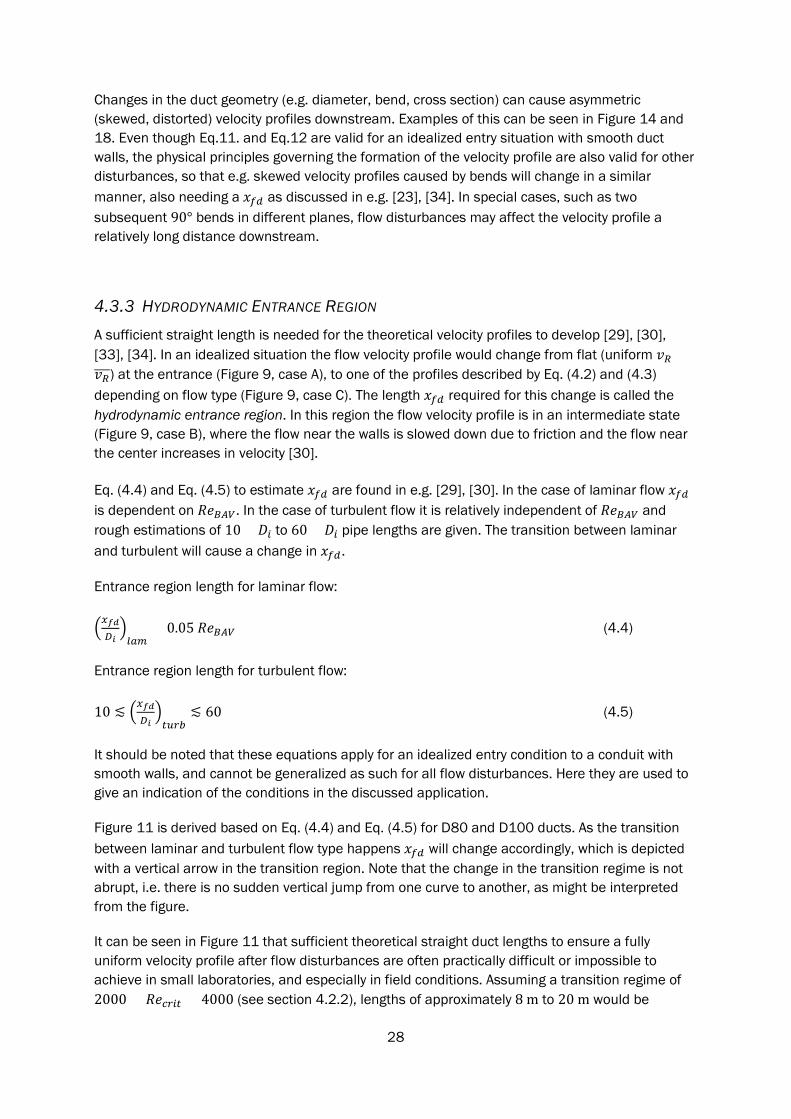
Changes in the duct geometry (e.g. diameter, bend, cross section) can cause asymmetric (skewed, distorted) velocity profiles downstream. Examples of this can be seen in Figure 14 and 18. Even though Eq.11. and Eq.12 are valid for an idealized entry situation with smooth duct walls, the physical principles governing the formation of the velocity profile are also valid for other disturbances, so that e.g. skewed velocity profiles caused by bends will change in a similar manner, also needing a 𝑥𝑥𝑓𝑓𝑑𝑑 as discussed in e.g. [23], [34]. In special cases, such as two subsequent 90° bends in different planes, flow disturbances may affect the velocity profile a relatively long distance downstream.

4.3.3 HYDRODYNAMIC ENTRANCE REGION A sufficient straight length is needed for the theoretical velocity profiles to develop [29], [30], [33], [34]. In an idealized situation the flow velocity profile would change from flat (uniform 𝑣𝑣𝑅𝑅 =𝑣𝑣𝑅𝑅���) at the entrance (Figure 9, case A), to one of the profiles described by Eq. (4.2) and (4.3) depending on flow type (Figure 9, case C). The length 𝑥𝑥𝑓𝑓𝑑𝑑 required for this change is called the hydrodynamic entrance region. In this region the flow velocity profile is in an intermediate state (Figure 9, case B), where the flow near the walls is slowed down due to friction and the flow near the center increases in velocity [30].

Eq. (4.4) and Eq. (4.5) to estimate 𝑥𝑥𝑓𝑓𝑑𝑑 are found in e.g. [29], [30]. In the case of laminar flow 𝑥𝑥𝑓𝑓𝑑𝑑 is dependent on 𝑅𝑅𝑅𝑅𝐵𝐵𝐵𝐵𝐵𝐵. In the case of turbulent flow it is relatively independent of 𝑅𝑅𝑅𝑅𝐵𝐵𝐵𝐵𝐵𝐵 and rough estimations of 10 × 𝐷𝐷𝑖𝑖 to 60 × 𝐷𝐷𝑖𝑖 pipe lengths are given. The transition between laminar and turbulent will cause a change in 𝑥𝑥𝑓𝑓𝑑𝑑.

Entrance region length for laminar flow:

�𝑥𝑥𝑓𝑓𝑑𝑑𝑃𝑃𝑖𝑖�𝑙𝑙𝑙𝑙𝑚𝑚

= 0.05 𝑅𝑅𝑅𝑅𝐵𝐵𝐵𝐵𝐵𝐵 (4.4)

Entrance region length for turbulent flow:

10 ≲ �𝑥𝑥𝑓𝑓𝑑𝑑𝑃𝑃𝑖𝑖�𝑡𝑡𝑡𝑡𝑐𝑐𝑡𝑡

≲ 60 (4.5)

It should be noted that these equations apply for an idealized entry condition to a conduit with smooth walls, and cannot be generalized as such for all flow disturbances. Here they are used to give an indication of the conditions in the discussed application.

Figure 11 is derived based on Eq. (4.4) and Eq. (4.5) for D80 and D100 ducts. As the transition between laminar and turbulent flow type happens 𝑥𝑥𝑓𝑓𝑑𝑑 will change accordingly, which is depicted with a vertical arrow in the transition region. Note that the change in the transition regime is not abrupt, i.e. there is no sudden vertical jump from one curve to another, as might be interpreted from the figure.

It can be seen in Figure 11 that sufficient theoretical straight duct lengths to ensure a fully uniform velocity profile after flow disturbances are often practically difficult or impossible to achieve in small laboratories, and especially in field conditions. Assuming a transition regime of 2000 < 𝑅𝑅𝑅𝑅𝑐𝑐𝑐𝑐𝑖𝑖𝑡𝑡 < 4000 (see section 4.2.2), lengths of approximately 8 m to 20 m would be

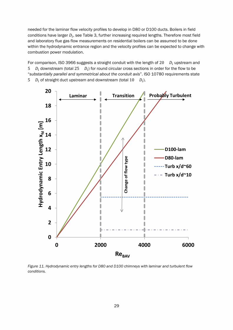
29

needed for the laminar flow velocity profiles to develop in D80 or D100 ducts. Boilers in field conditions have larger 𝐷𝐷𝑖𝑖, see Table 3, further increasing required lengths. Therefore most field and laboratory flue gas flow measurements on residential boilers can be assumed to be done within the hydrodynamic entrance region and the velocity profiles can be expected to change with combustion power modulation.

For comparison, ISO 3966 suggests a straight conduit with the length of 20 × 𝐷𝐷𝑖𝑖 upstream and 5 × 𝐷𝐷𝑖𝑖 downstream (total 25 × 𝐷𝐷𝑖𝑖) for round circular cross sections in order for the flow to be “substantially parallel and symmetrical about the conduit axis”. ISO 10780 requirements state 5 × 𝐷𝐷𝑖𝑖 of straight duct upstream and downstream (total 10 × 𝐷𝐷𝑖𝑖).

Figure 11. Hydrodynamic entry lengths for D80 and D100 chimneys with laminar and turbulent flow conditions.

0

2

4

6

8

10

12

14

16

18

20

0 2000 4000 6000

Hydr

odyn

amic

Ent

ry L

engt

h x f

d[m

]

ReBAV

D100-lam

D80-lam

Turb x/d~60

Turb x/d~10

Laminar Transition Probably Turbulent

Chan

ge o

f flo

w ty

pe

30

4.3.4 SINGLE POINT VELOCITY MEASUREMENT METHODS

The standards ISO 3966 and ISO 10780 use a traversing sampling method to take into account the actual flow velocity profile. There are also methods for determining the flow rate in a round duct with a single point measurement, two of which are briefly presented here. These approaches, however, are valid only for fully developed (axisymmetric) velocity profiles and would not be of practical help in cases of skewed velocity profiles or in the hydrodynamic entrance region, for which the velocity profiles may also be changing as a function of 𝑅𝑅𝑅𝑅𝐵𝐵𝐵𝐵𝐵𝐵 (exemplified experimentally in section 4.3.5).

Center point method

A method for measuring the flow rate with a single center (or arbitrary) point measurement would be to use the pipe factor, as described in [23]. The method is based on the fact that the velocity profile in fully developed flows is a function of pipe surface roughness and 𝑅𝑅𝑅𝑅𝐵𝐵𝐵𝐵𝐵𝐵 and can thus be predicted with the help of the Moody’s diagram. Eq. (4.2) and Eq. (4.3) are a simplification of this method. The method is limited to fully developed velocity profiles and the flow type must be known.

As an example, if a single point measurement is done at the center of the duct (see Figure 10), it is of most importance to be certain if the velocity is either turbulent or laminar, otherwise a significant over or under estimation by a factor of 2.00/1.25 ≈ 1.6 is possible.

The center point measurement is recommended for duct diameters relatively small compared to the probe, where positioning the probe closer to the wall (e.g. at the critical point as described next) would result in undesirable effects due to wall proximity [16], but the method is usable if there is no change in flow characteristic or if both the change and velocity profiles are always predictable.

Three quarter radius method

There is a method for partially taking into account the change in velocity profile using a single measurement point on the radius where the impact of the profile change is at minimum. A horizontal dashed line is drawn in Figure 10 at 𝑣𝑣𝑅𝑅𝑐𝑐 𝑣𝑣𝑅𝑅��� = 1⁄ representing the average bulk velocity. For either the turbulent or laminar case, where 𝑣𝑣𝑅𝑅𝑐𝑐 𝑣𝑣𝑅𝑅��� = 1⁄ (i.e. where 𝑣𝑣𝑅𝑅𝑐𝑐 curve crosses the horizontal dashed line) gives for each case the 𝑅𝑅𝑐𝑐 where a 𝑣𝑣𝑅𝑅 corresponding to the 𝑣𝑣𝑅𝑅��� can be measured. This 𝑅𝑅𝑐𝑐 is in some literature sources called the critical position, e.g. [16], [23], or three quarter radius, e.g. [14], [35].

In the case presented in Figure 10, the critical position for the laminar flow is at 𝑅𝑅𝑐𝑐 ≈ 0.71 and for turbulent at 𝑅𝑅𝑐𝑐 ≈ 0.75. A critical position for measuring the average bulk velocity taking into account both laminar and turbulent velocity profiles with minimal error would be 𝑅𝑅𝑐𝑐 ≈ 0.73, where theoretically the measurement would underestimate laminar 𝑣𝑣𝑅𝑅��� by 5 % and overestimate turbulent 𝑣𝑣𝑅𝑅��� by 3 %, approximately.

31

4.3.5 MEASURED CHIMNEY FLOW VELOCITY PROFILES

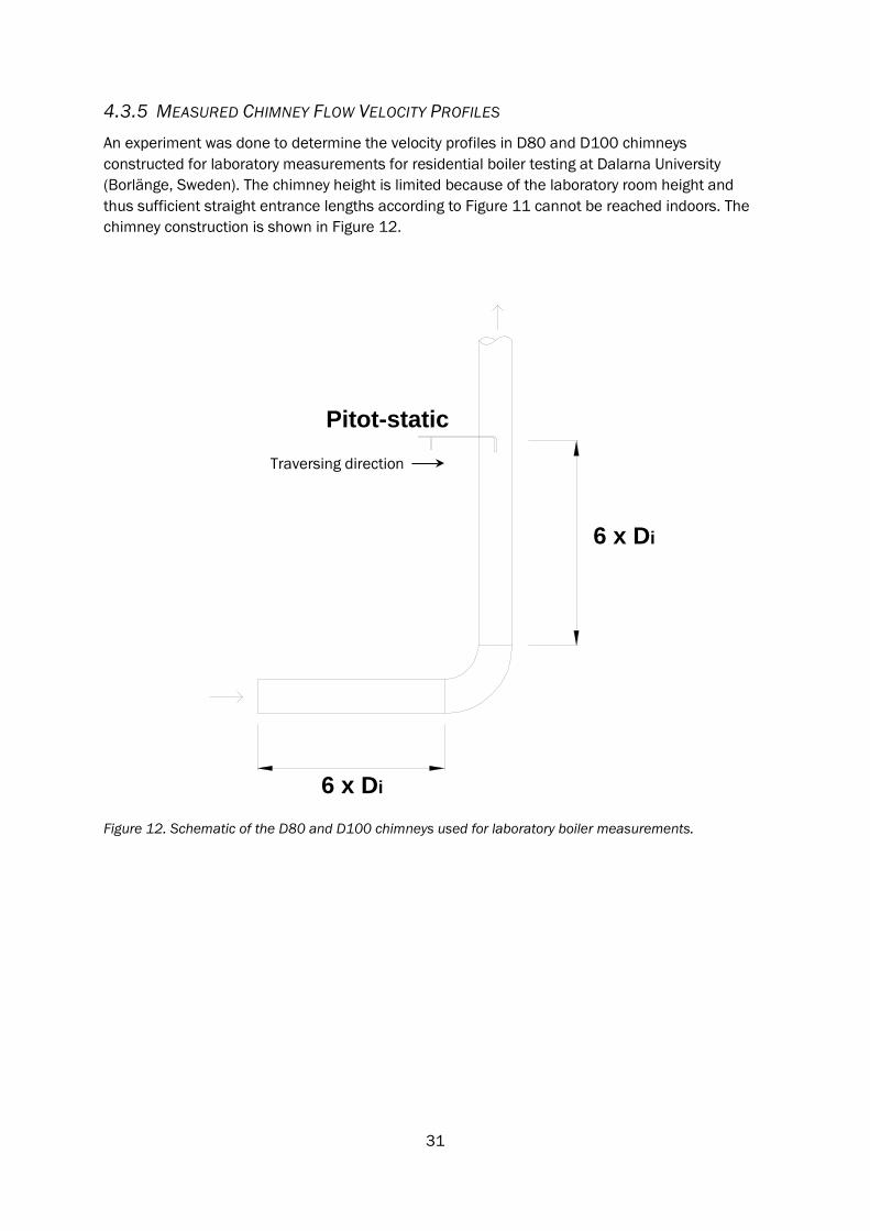
An experiment was done to determine the velocity profiles in D80 and D100 chimneys constructed for laboratory measurements for residential boiler testing at Dalarna University (Borlänge, Sweden). The chimney height is limited because of the laboratory room height and thus sufficient straight entrance lengths according to Figure 11 cannot be reached indoors. The chimney construction is shown in Figure 12.

Figure 12. Schematic of the D80 and D100 chimneys used for laboratory boiler measurements.

Pitot-static

6 x Di

p

6 x Di

Traversing direction

32

Measurement conditions:

• Air at room temperature was used. • The velocity profile measurement was done with a Pitot-static probe (standard 𝑑𝑑𝑝𝑝𝑝𝑝 =

4 mm L-type). Note that 𝑑𝑑𝑝𝑝𝑝𝑝 = 4 mm is actually larger than the ISO 3699 or ISO 10780 allow for these duct diameters as a smaller diameter probe was not available in the laboratory. This is not critical for the conclusions.

• The traversing was done through seven (D80) and ten (D100) sampling points on a single diameter of the duct cross section. The traversing direction is shown in figure 8.

• Each sample is an average of 3 minutes of steady state flow sampled with a 10 second sampling interval.

• A stand with a guiding rail was built for the probe to ensure minimal differences in probe alignment with the flow between the traverses. The reference flow rate was measured with a set of calibrated orifice plates, see section 8.1.

The measured velocity profiles are shown in Figures 13 and 14. The velocities at the wall (for 𝑅𝑅𝑐𝑐 = 1 and 𝑅𝑅𝑐𝑐 = −1) are assumed 0. The measurements were done at several 𝑅𝑅𝑅𝑅𝐵𝐵𝐵𝐵𝐵𝐵, but for clarity only the two extremes and an intermediate are shown in Figures 13 and 14. The observed velocity profile changes were gradual and consistent with literature [30].

Comparing the measured velocity profiles to Figures 9 and 10 it can be seen that in both chimneys the velocity profile changes from a turbulent type towards a laminar (parabolic) one, due to flow type change. It can also be seen that the velocity profile is skewed when turbulent, approaching symmetric when laminar, but does not reach a fully parabolic state with laminar flow, due to insufficient entrance length.

These measurements show that the theoretical velocity profile effects discussed in sections 4.3.1-4.3.3 are present in the duct, and should therefore be taken into account in chimney flue gas flow rate measurements.

As an example, in both the measured cases of Figures 13 and 14, there is approximately an 11 % difference between the turbulent and laminar average velocities using the center point velocity as a reference. This would contribute to the uncertainty of a continuous measurement with the often used center point method, see section 4.3.4.

Because the measurement was performed only at room temperature it should be noted that the viscosity is a function of temperature, and thus 𝑅𝑅𝑅𝑅𝐵𝐵𝐵𝐵𝐵𝐵 of flue gas varies also with temperature. Expected 𝑅𝑅𝑅𝑅𝐵𝐵𝐵𝐵𝐵𝐵 in chimneys for comparison can be found e.g. in Figure 7 and 8.

The results also give an indication that the ISO 10780 requirements of 5 × 𝐷𝐷𝑖𝑖 of straight duct upstream and downstream are not sufficient to achieve a symmetric velocity profile.

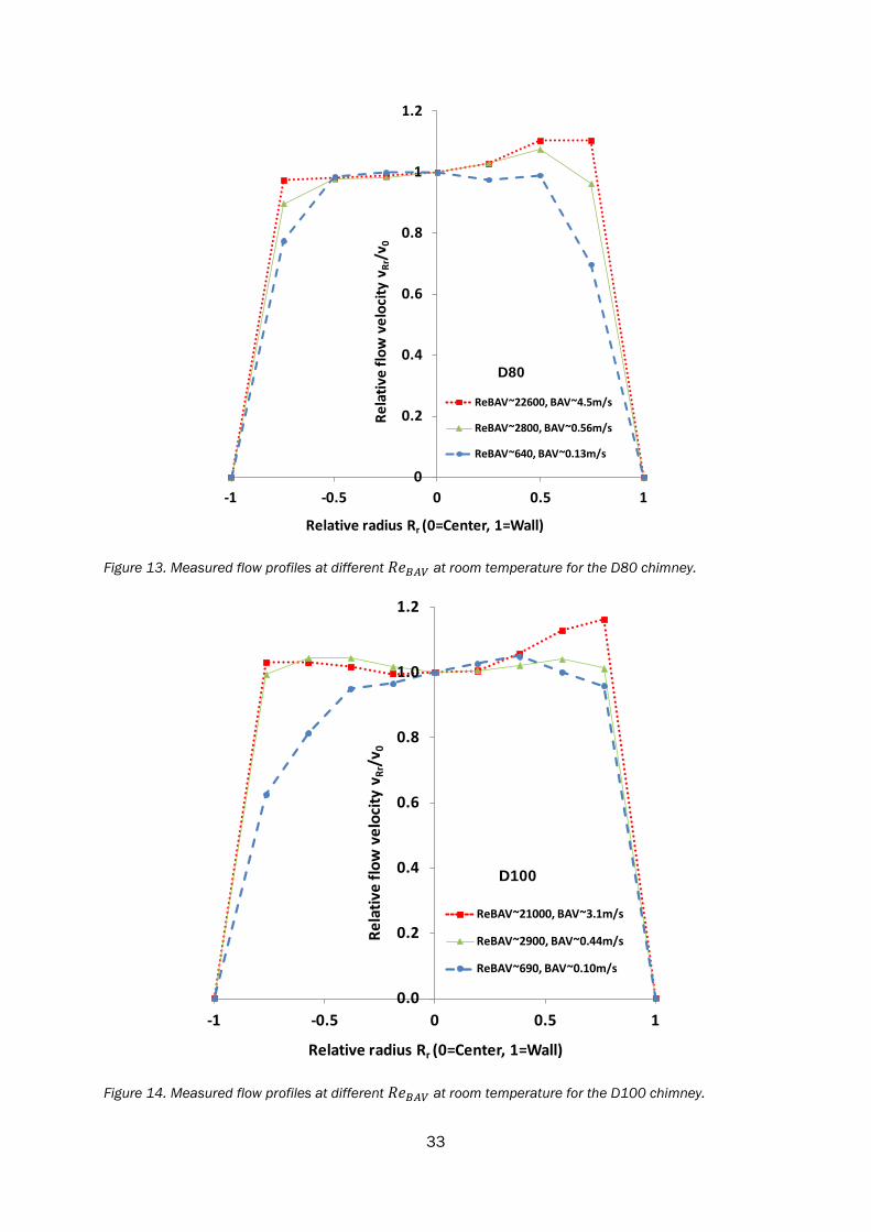
33

Figure 13. Measured flow profiles at different 𝑅𝑅𝑅𝑅𝐵𝐵𝐵𝐵𝐵𝐵 at room temperature for the D80 chimney.

Figure 14. Measured flow profiles at different 𝑅𝑅𝑅𝑅𝐵𝐵𝐵𝐵𝐵𝐵 at room temperature for the D100 chimney.

0

0.2

0.4

0.6

0.8

1

1.2

-1 -0.5 0 0.5 1

Rela

tive

flow

vel

ocity

vRr

/v0

Relative radius Rr (0=Center, 1=Wall)

ReBAV~22600, BAV~4.5m/s

ReBAV~2800, BAV~0.56m/s

ReBAV~640, BAV~0.13m/s

D80

0.0

0.2

0.4

0.6

0.8

1.0

1.2

-1 -0.5 0 0.5 1

Rela

tive

flow

vel

ocity

vRr

/v0

Relative radius Rr (0=Center, 1=Wall)

ReBAV~21000, BAV~3.1m/s

ReBAV~2900, BAV~0.44m/s

ReBAV~690, BAV~0.10m/s

D100

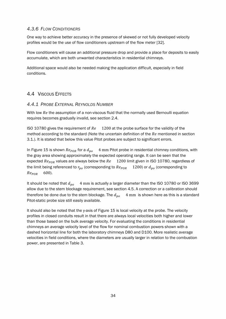
34

4.3.6 FLOW CONDITIONERS

One way to achieve better accuracy in the presence of skewed or not fully developed velocity profiles would be the use of flow conditioners upstream of the flow meter [32].

Flow conditioners will cause an additional pressure drop and provide a place for deposits to easily accumulate, which are both unwanted characteristics in residential chimneys.

Additional space would also be needed making the application difficult, especially in field conditions.

4.4 VISCOUS EFFECTS

4.4.1 PROBE EXTERNAL REYNOLDS NUMBER

With low 𝑅𝑅𝑅𝑅 the assumption of a non-viscous fluid that the normally used Bernoulli equation requires becomes gradually invalid, see section 2.4.

ISO 10780 gives the requirement of 𝑅𝑅𝑅𝑅 > 1200 at the probe surface for the validity of the method according to the standard (Note the uncertain definition of the 𝑅𝑅𝑅𝑅 mentioned in section 3.1.). It is stated that below this value Pitot probes are subject to significant errors.

In Figure 15 is shown 𝑅𝑅𝑅𝑅𝑃𝑃𝑃𝑃𝑅𝑅 for a 𝑑𝑑𝑝𝑝𝑝𝑝 = 4 mm Pitot probe in residential chimney conditions, with the gray area showing approximately the expected operating range. It can be seen that the expected 𝑅𝑅𝑅𝑅𝑃𝑃𝑃𝑃𝑅𝑅 values are always below the 𝑅𝑅𝑅𝑅 > 1200 limit given in ISO 10780, regardless of the limit being referenced to 𝑟𝑟𝑝𝑝𝑝𝑝 (corresponding to 𝑅𝑅𝑅𝑅𝑃𝑃𝑃𝑃𝑅𝑅 > 1200) or 𝑑𝑑𝑝𝑝𝑝𝑝 (corresponding to 𝑅𝑅𝑅𝑅𝑃𝑃𝑃𝑃𝑅𝑅 > 600).

It should be noted that 𝑑𝑑𝑝𝑝𝑝𝑝 = 4 mm is actually a larger diameter than the ISO 10780 or ISO 3699 allow due to the stem blockage requirement, see section 4.5. A correction or a calibration should therefore be done due to the stem blockage. The 𝑑𝑑𝑝𝑝𝑝𝑝 = 4 mm is shown here as this is a standard Pitot-static probe size still easily available.

It should also be noted that the y-axis of Figure 15 is local velocity at the probe. The velocity profiles in closed conduits result in that there are always local velocities both higher and lower than those based on the bulk average velocity. For evaluating the conditions in residential chimneys an average velocity level of the flow for nominal combustion powers shown with a dashed horizontal line for both the laboratory chimneys D80 and D100. More realistic average velocities in field conditions, where the diameters are usually larger in relation to the combustion power, are presented in Table 3.

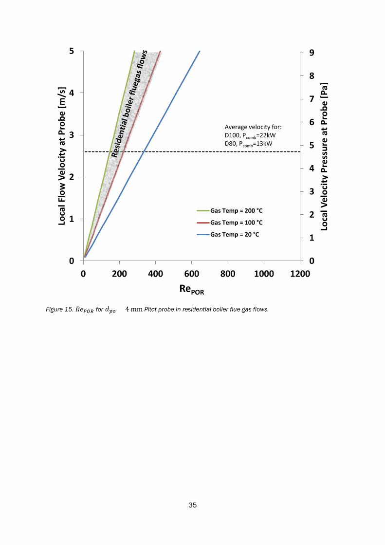
35

Figure 15. 𝑅𝑅𝑅𝑅𝑃𝑃𝑃𝑃𝑅𝑅 for 𝑑𝑑𝑝𝑝𝑝𝑝 = 4 mm Pitot probe in residential boiler flue gas flows.

0

1

2

3

4

5

6

7

8

9

0

1

2

3

4

5

0 200 400 600 800 1000 1200

Loca

l Vel

ocity

Pre

ssur

e at

Pro

be [P

a]

Loca

l Flo

w V

eloc

ity a

t Pro

be [m

/s]

RePOR

Gas Temp = 200 °C

Gas Temp = 100 °C

Gas Temp = 20 °C

Average velocity for:D100, Pcomb=22kWD80, Pcomb=13kW

36

4.4.2 PROBE STAGNATION PRESSURE PORT REYNOLDS NUMBER

There is also a requirement 𝑅𝑅𝑅𝑅𝑃𝑃𝑃𝑃𝑅𝑅 > 100 set in ISO 3966 (Note: In the reference the limit is 𝑅𝑅𝑅𝑅 >200 based on impact hole internal diameter, but the praxis to compare research results has mostly been radius.). The reason for this requirement is not explained in the standard, but based on the given literature reference [16] it is because at lower 𝑅𝑅𝑅𝑅𝑃𝑃𝑃𝑃𝑅𝑅 viscous effects in the pressure passages of the probe start causing both a measurement error similarly to the probe external conditions (see section 4.4.1), and significant time lag in the probe response [16], [22].

In Figure 16 is shown the 𝑅𝑅𝑅𝑅𝑃𝑃𝑃𝑃𝑅𝑅 for a 𝑑𝑑𝑝𝑝𝑖𝑖 = 1.6 mm (a normal size for a 𝑑𝑑𝑝𝑝𝑝𝑝 = 4 mm L-type Pitot-Static probe) impact pressure tube under chimney conditions, with the gray area showing approximately the expected operating range of a boiler. The calculated average values are below the given requirement 𝑅𝑅𝑅𝑅𝑃𝑃𝑃𝑃𝑅𝑅 > 100.

It should be noted that y-axis of Figure 16 is local velocity at the probe. The velocity profiles in closed conduits result in that there are always local velocities both higher and lower than those based on the bulk average velocity. For evaluating the conditions in residential chimneys an average velocity level of the flow for nominal combustion powers shown with a dashed horizontal line for both the laboratory chimneys D80 and D100. More realistic average velocities in field conditions, where the diameters are usually larger in relation to the combustion power, are presented in Table 3.

No detailed description of the time lag caused by viscosity was found in the available literature. A short description in [22] summarizes that the time constants are dependent on the diameters and lengths of the probe pressure passages and the displacement volume of the manometer and related connections, and are very short for down to 𝑑𝑑𝑝𝑝𝑝𝑝 = 3 mm probes, but for smaller probes in the order of tens of seconds to minutes. (It is actually not clearly stated in the reference whether used acronym o.d. refers to outer or orifice diameter, but judging based on praxis and references, e.g. [36], the acronym is normally used for the former.) The time constants of standard sized Pitot-static probes in low flow velocities are not discussed, however.

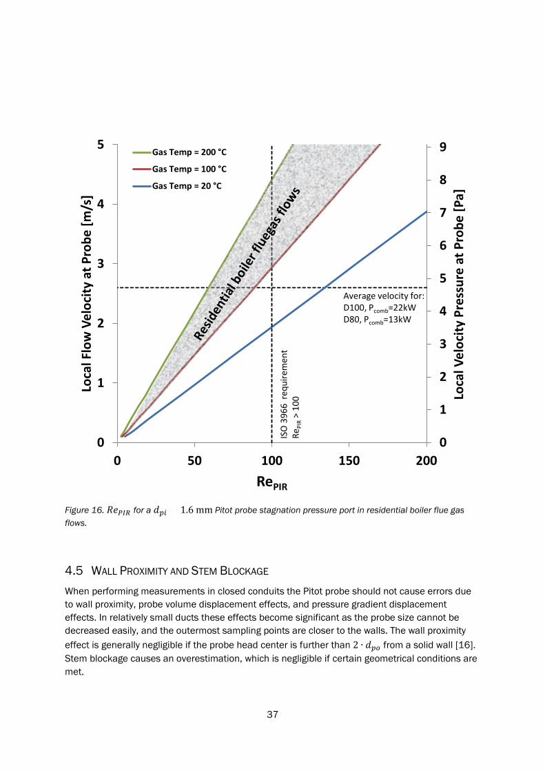
37

Figure 16. 𝑅𝑅𝑅𝑅𝑃𝑃𝑃𝑃𝑅𝑅 for a 𝑑𝑑𝑝𝑝𝑖𝑖 = 1.6 mm Pitot probe stagnation pressure port in residential boiler flue gas flows.

4.5 WALL PROXIMITY AND STEM BLOCKAGE When performing measurements in closed conduits the Pitot probe should not cause errors due to wall proximity, probe volume displacement effects, and pressure gradient displacement effects. In relatively small ducts these effects become significant as the probe size cannot be decreased easily, and the outermost sampling points are closer to the walls. The wall proximity effect is generally negligible if the probe head center is further than 2 ∙ 𝑑𝑑𝑝𝑝𝑝𝑝 from a solid wall [16]. Stem blockage causes an overestimation, which is negligible if certain geometrical conditions are met.

0

1

2

3

4

5

6

7

8

9

0

1

2

3

4

5

0 50 100 150 200Lo

cal V

eloc

ity P

ress

ure

at P

robe

[Pa]

Loca

l Flo

w V

eloc

ity a

t Pro

be [m

/s]

RePIR

Gas Temp = 200 °C

Gas Temp = 100 °C

Gas Temp = 20 °C

Average velocity for:D100, Pcomb=22kWD80, Pcomb=13kW

ISO

3966

req

uire

men

t Re

PIR

> 10

0

38

A dimensional limit of 𝑑𝑑𝑝𝑝𝑝𝑝 𝐷𝐷𝑖𝑖⁄ < 0.02 is set in ISO 3966, after which a correction should be done. ISO 3699 provides a correction method and a summary is given also in [21], [22]. In ISO 10780 this requirement has been translated to an internal cross sectional area limit of 𝐴𝐴𝑖𝑖 < 0.07 m2 of the duct for the method to be valid, giving a minimum of 𝐷𝐷𝑖𝑖 ≈ 300 mm for round ducts. This is in accordance with Ower stating that an 𝑑𝑑𝑝𝑝𝑝𝑝 = 8 mm Pitot probe should not be used in 𝐷𝐷𝑖𝑖 <300 mm ducts for traversing measurements [16].

Residential heating boiler and stove flue gas ducts and chimneys range normally from 80 < 𝐷𝐷𝑖𝑖 <150 mm, meaning that the ISO 10780 and ISO 3699 methods and uncertainties are not valid as such regarding these requirements.

As an example, if a 0.5 % maximum error of the differential pressure due to these effects is allowed, 𝑑𝑑𝑝𝑝𝑝𝑝 should not be greater than 1.6 mm for D80 and 2.0 mm for D100 chimneys. These probe sizes are not readily available, and thus more easily found standard size probes with 𝑑𝑑𝑝𝑝𝑝𝑝 =4 mm to 𝑑𝑑𝑝𝑝𝑝𝑝 = 8 mm would require either theoretical error correction or in situ calibration. Small diameters may also start suffering from significant time lag in their response times, see section 4.4.2, although this characteristic needs to be tested experimentally specifically for low 𝑅𝑅𝑅𝑅 flows.

4.6 FLUE GAS DENSITY The fluid density is used both in the Bernoulli equation and when converting between volume and mass flow rates. According to ISO 10780 and ISO 3699 a correction for density has to be done if the gas density is suspected to be significantly different to that of air. The flue gas composition is usually known and the density can easily be accounted for.

Especially with wet biomass with moisture contents greater than 20 % (wet basis) over +5 % differences in density compared to air may occur, depending also on the combustion excess air ratio. For wood pellets the moisture content is normally below 10 % (wet basis). With a moisture content of 7 % (wet basis) and 𝜆𝜆 = 2 the difference in density is +0.9 %.

4.7 AVERAGE FLOW TEMPERATURE The flue gas temperature during normal boiler operation can vary from 100 °C to 200 °C, see section 4.1. During startup and stop sequences and leakage flows, temperatures down to near ambient may be present, although the boiler water temperature normally sets the lower limit. For measurements of transient characteristics the mentioned temperature range can be present.

In the traversing method according to ISO 10780, the absolute temperature of each measurement point should not differ more than 5 % from the average absolute temperature in the measurement cross section. This translates to ±19 °C at 80 °C and ±24 °C at 200 °C average flue gas temperature, which corresponds to a ±2.5 % uncertainty in the determination of the flow rate in both cases.

In continuous measurements of transient flows, when traversing is not done, care must be taken to measure a representative average bulk temperature. Based on field and laboratory

39

measurement experience of the author, the local temperatures in a flue gas duct can vary significantly (in extreme cases tens of °C) over the cross section depending on various factors, such as distance from the boiler outlet, boiler construction, insulation of the duct, combustion power modulation rate, flow type, and vertical or horizontal alignment of the duct. A temperature profile may be preserved for relatively long distances even in vertical ducts if the flow is partially laminar, and similarly to the velocity profile, the temperature profile can also change dependent on the flow rate and type.

Thus for continuous measurements of transient flows a single point temperature measurement may not be sufficient, if a consistent representative bulk average temperature cannot be confirmed for the whole operating range. Vertical ducts should be preferred to prevent natural density stratification due to heat losses through the walls.

4.8 YAW ANGLE Misalignment of the Pitot probe with respect to the flow direction (yaw angle) causes measurement errors [14], [16], [21], for which static ports are more sensitive than total pressure ports. For a Pitot-static probe a maximum of ±5 % impact pressure deviation can be assumed within 30° yaw angle and less than +2 % if the yaw angle is kept under 5°. These error estimations are under normal measurement conditions and it is mentioned that the they are slightly dependent on the 𝑅𝑅𝑅𝑅𝑃𝑃𝑃𝑃𝑅𝑅 [14], but the sources do not specifically discuss the case of laminar flows, or cases where viscous effects may not be negligible.

A fixed stand with a locking system to fix the probe always in the same position is an easy and feasible solution for minimizing alignment errors in cases where the probe often needs to be taken out e.g. for cleaning.

4.9 VIBRATIONS Errors because of probe vibration [16] are unlikely to disturb measurements in residential chimney conditions. Fluid flow velocities are not high enough to induce vibrations to the probe and devices causing significant enough mechanical vibrations transferred via duct walls are unlikely.

4.10 TURBULENCE Turbulence may cause additional pressure difference sensed between the impact and static ports of the probe, i.e. it leads to overestimation of the velocity pressure. Ower [16] summarizes that the turbulence intensities in industrial applications will have negligible effects. Based on the correction method presented in ISO 3699 the overestimation is 0.5 % at most.

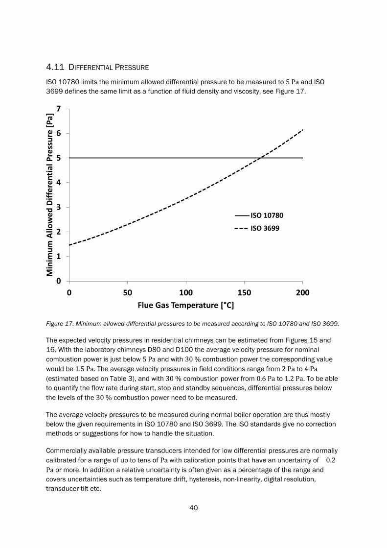
40

4.11 DIFFERENTIAL PRESSURE ISO 10780 limits the minimum allowed differential pressure to be measured to 5 Pa and ISO 3699 defines the same limit as a function of fluid density and viscosity, see Figure 17.

Figure 17. Minimum allowed differential pressures to be measured according to ISO 10780 and ISO 3699.

The expected velocity pressures in residential chimneys can be estimated from Figures 15 and 16. With the laboratory chimneys D80 and D100 the average velocity pressure for nominal combustion power is just below 5 Pa and with 30 % combustion power the corresponding value would be 1.5 Pa. The average velocity pressures in field conditions range from 2 Pa to 4 Pa (estimated based on Table 3), and with 30 % combustion power from 0.6 Pa to 1.2 Pa. To be able to quantify the flow rate during start, stop and standby sequences, differential pressures below the levels of the 30 % combustion power need to be measured.

The average velocity pressures to be measured during normal boiler operation are thus mostly below the given requirements in ISO 10780 and ISO 3699. The ISO standards give no correction methods or suggestions for how to handle the situation.

Commercially available pressure transducers intended for low differential pressures are normally calibrated for a range of up to tens of Pa with calibration points that have an uncertainty of ±0.2 Pa or more. In addition a relative uncertainty is often given as a percentage of the range and covers uncertainties such as temperature drift, hysteresis, non-linearity, digital resolution, transducer tilt etc.

0

1

2

3

4

5

6

7

0 50 100 150 200

Min

imum

Allo

wed

Diff

eren

tial P

ress

ure

[Pa]

Flue Gas Temperature [°C]

ISO 10780

ISO 3699

41

For example, a typical transducer with a range of 0 Pa to 30 Pa and an uncertainty of 2 % of the range cannot be trusted to give useful data below a resolution of 0.6 Pa according to the specifications and standard calibration. This is in the same order of magnitude as the differential pressures to be measured during minimum combustion power modulation.

Differential pressure transducers are also discussed in section 7.

4.12 OTHER CONSIDERATIONS Both the temperature range and chemical conditions in flue gases put requirements on the used sensor construction materials.

Flue gases from a boiler contain also particulate matter, soot and ash, which can easily clog the sensor. Condensing fluids, e.g. water and tar evaporated from the fuel, usually worsen the clogging. This sets requirements for being able to dismount, clean, and mount the probe often and quickly without causing a need for recalibration. Preferably the cleaning should also be possible during boiler operation.

Heat conductance from the probe to the ambient should be minimized by material choice and insulation on the outside to prevent water vapor condensation from the flue gas flow on to the probe surface and condensation in the connecting tubes.

Especially in field conditions the flow measurement method should not cause a significant irrecoverable pressure drop, as this would most likely prevent a natural chimney draft based boiler from operating normally. Even in laboratory conditions it is beneficial to be able to use a method which causes only a low irrecoverable pressure drop to the flow, both because of exhaust gas fan sizing and the possibility to emulate natural chimney draft conditions for a boiler.

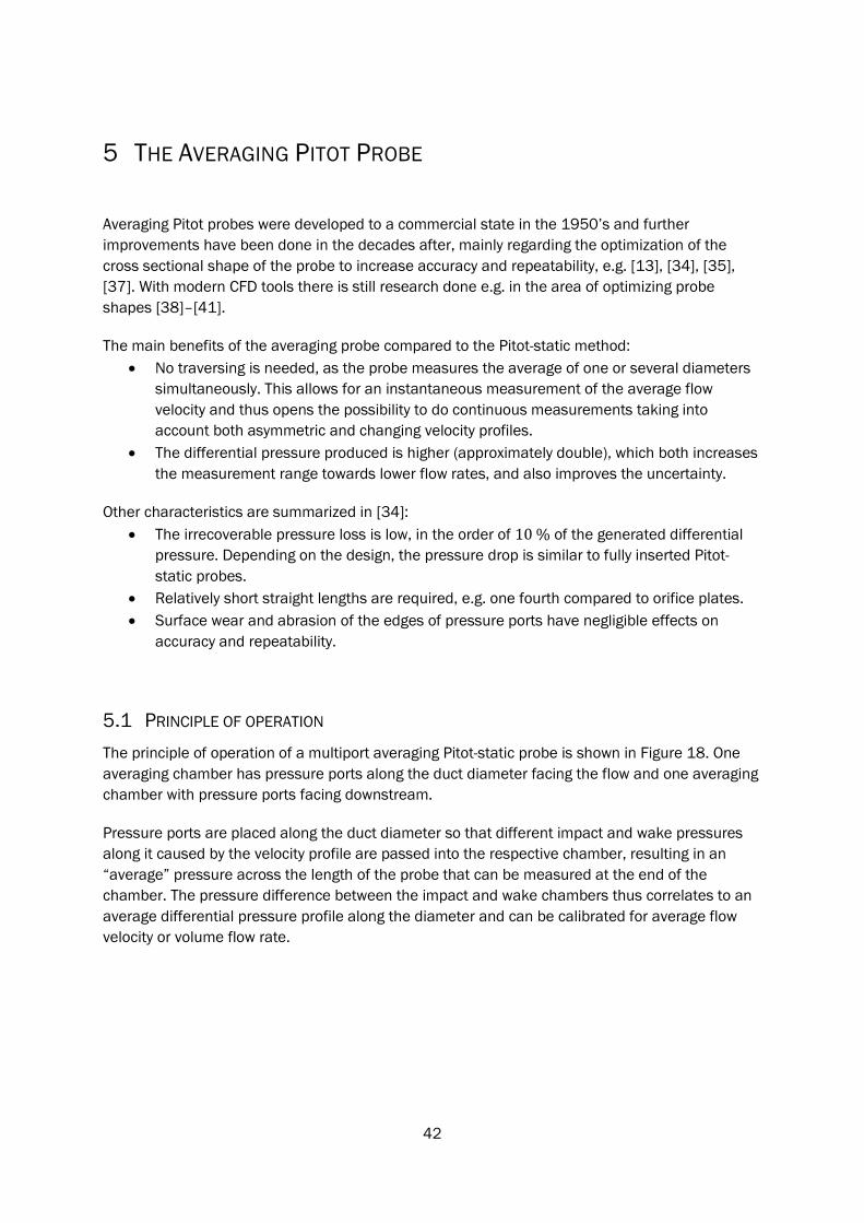
42

5 THE AVERAGING PITOT PROBE

Averaging Pitot probes were developed to a commercial state in the 1950’s and further improvements have been done in the decades after, mainly regarding the optimization of the cross sectional shape of the probe to increase accuracy and repeatability, e.g. [13], [34], [35], [37]. With modern CFD tools there is still research done e.g. in the area of optimizing probe shapes [38]–[41].

The main benefits of the averaging probe compared to the Pitot-static method: • No traversing is needed, as the probe measures the average of one or several diameters

simultaneously. This allows for an instantaneous measurement of the average flow velocity and thus opens the possibility to do continuous measurements taking into account both asymmetric and changing velocity profiles.

• The differential pressure produced is higher (approximately double), which both increases the measurement range towards lower flow rates, and also improves the uncertainty.

Other characteristics are summarized in [34]: • The irrecoverable pressure loss is low, in the order of 10 % of the generated differential

pressure. Depending on the design, the pressure drop is similar to fully inserted Pitot-static probes.

• Relatively short straight lengths are required, e.g. one fourth compared to orifice plates. • Surface wear and abrasion of the edges of pressure ports have negligible effects on

accuracy and repeatability.

5.1 PRINCIPLE OF OPERATION The principle of operation of a multiport averaging Pitot-static probe is shown in Figure 18. One averaging chamber has pressure ports along the duct diameter facing the flow and one averaging chamber with pressure ports facing downstream.

Pressure ports are placed along the duct diameter so that different impact and wake pressures along it caused by the velocity profile are passed into the respective chamber, resulting in an “average” pressure across the length of the probe that can be measured at the end of the chamber. The pressure difference between the impact and wake chambers thus correlates to an average differential pressure profile along the diameter and can be calibrated for average flow velocity or volume flow rate.

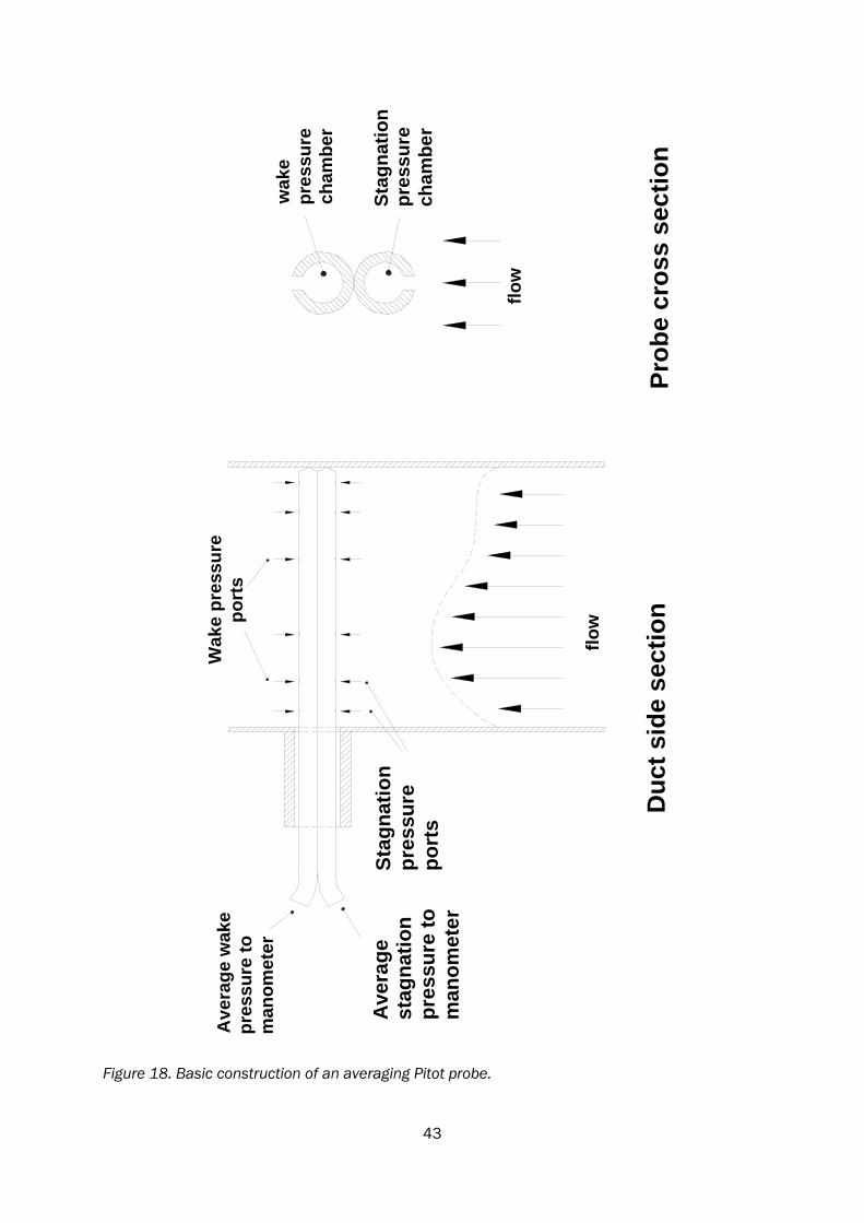
43

Figure 18. Basic construction of an averaging Pitot probe.

impa

ctpr

essu

rech

ambe

r

wak

epr

essu

rech

ambe

r

Prob

e cr

oss

sect

ion

flow

Impa

ctpr

essu

repo

rts

Wak

e pr

essu

repo

rts

Duc

t sid

e se

ctio

n

flow

Ave

rage

wak

epr

essu

re to

man

omet

er

Ave

rage

impa

ct

pres

sure

tom

anom

eter

Stag

natio

n pr

essu

re

port

s

Ave

rage

st

agna

tion

pres

sure

to

man

omet

er

Stag

natio

n pr

essu

re

cham

ber

44

Several probes can be used so that an average pressure across multiple diameters is measured simultaneously by the manometer, if asymmetric and/or changing velocity profiles are expected.

It should be noted that, depending on the design, the differential pressure produced is higher (normally approximately double) than that produced by e.g. a standard L-type Pitot-static probe. This is because the wake pressure is lower than the static pressure, see section 5.2.2. The wake pressure is dependent on the probe cross section and 𝑅𝑅𝑅𝑅𝑃𝑃𝑃𝑃𝑅𝑅, e.g. [13], [30]. The static pressure, measured e.g. at the conduit wall, could also be used instead of the wake pressure, probably resulting in a simpler correlation, but this would result in lower (approximately halved) differential pressures, e.g. [13], [35], [42]. Reducing the produced differential pressure would be a significant disadvantage because of pressure transducer limitations, specifically when optimizing low flow rate performance, see section 7.

The shape of the sensor cross section and the placement of the pressure ports can be optimized in various ways for a higher and more stable and/or linear differential pressure over the intended operating range, e.g. [13], [37]–[41]. E.g. a diamond shape with sharp edges, as opposed to a cylinder, will separate the flow boundary layers from the probe surface always at the same position, resulting in a more stable wake pressure characteristic over a wider range of 𝑅𝑅𝑅𝑅. This leads to a more predictable wake pressure, making both the correlations and the calibration process simpler.

5.2 THEORY Cylinders of varying cross sectional shapes in cross flows have been extensively studied, especially for military naval and aviation applications. Zdradkovich has done a comprehensive summary on the topic in two books [43], [44].

5.2.1 DEFINITION OF REYNOLDS NUMBER FOR CYLINDERS

For cylinders in cross flows the Reynolds number has traditionally been defined based on the cylinder outer diameter. This is pointed out as it differs from the praxis of using the radius in the case of Pitot probes (see section 2.2) and therefore the subscript POD is used.

The 𝑅𝑅𝑅𝑅𝑃𝑃𝑃𝑃𝑃𝑃 is based either on • local flow velocity, which is the case of theoretical and experimental work where a uniform

velocity is considered along the length of the cylinder (two dimensional theory). • the average flow velocity in a duct, which is the case of a probe in a duct.

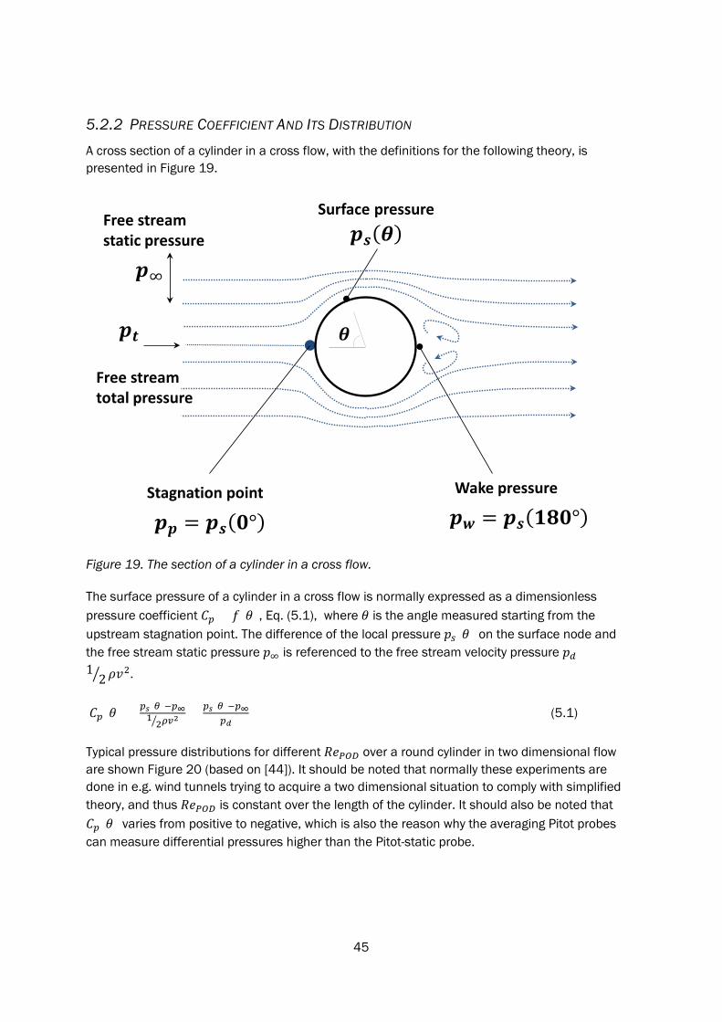
45

5.2.2 PRESSURE COEFFICIENT AND ITS DISTRIBUTION

A cross section of a cylinder in a cross flow, with the definitions for the following theory, is presented in Figure 19.

Figure 19. The section of a cylinder in a cross flow.

The surface pressure of a cylinder in a cross flow is normally expressed as a dimensionless pressure coefficient 𝐶𝐶𝑝𝑝 = 𝑓𝑓(𝜃𝜃), Eq. (5.1), where 𝜃𝜃 is the angle measured starting from the upstream stagnation point. The difference of the local pressure 𝑝𝑝𝑠𝑠(𝜃𝜃) on the surface node and the free stream static pressure 𝑝𝑝∞ is referenced to the free stream velocity pressure 𝑝𝑝𝑑𝑑 =1

2� 𝜌𝜌𝑣𝑣2.

𝐶𝐶𝑝𝑝(𝜃𝜃) = 𝑝𝑝𝑠𝑠(𝜃𝜃)−𝑝𝑝∞12� 𝜌𝜌𝜌𝜌2

= 𝑝𝑝𝑠𝑠(𝜃𝜃)−𝑝𝑝∞𝑝𝑝𝑑𝑑

(5.1)

Typical pressure distributions for different 𝑅𝑅𝑅𝑅𝑃𝑃𝑃𝑃𝑃𝑃 over a round cylinder in two dimensional flow are shown Figure 20 (based on [44]). It should be noted that normally these experiments are done in e.g. wind tunnels trying to acquire a two dimensional situation to comply with simplified theory, and thus 𝑅𝑅𝑅𝑅𝑃𝑃𝑃𝑃𝑃𝑃 is constant over the length of the cylinder. It should also be noted that 𝐶𝐶𝑝𝑝(𝜃𝜃) varies from positive to negative, which is also the reason why the averaging Pitot probes can measure differential pressures higher than the Pitot-static probe.

Free stream static pressure

Free stream total pressure

Stagnation point Wake pressure

Surface pressure

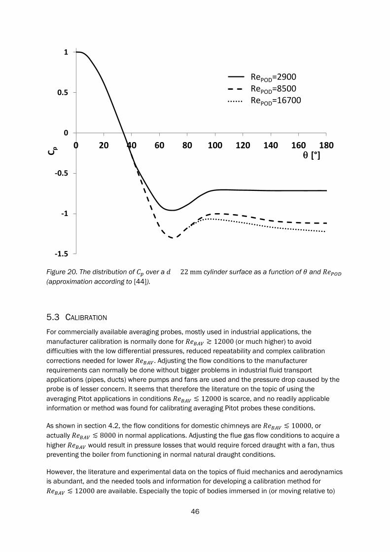
46

Figure 20. The distribution of 𝐶𝐶𝑝𝑝 over a 𝑑𝑑 = 22 mm cylinder surface as a function of 𝜃𝜃 and 𝑅𝑅𝑅𝑅𝑃𝑃𝑃𝑃𝑃𝑃 (approximation according to [44]).

5.3 CALIBRATION For commercially available averaging probes, mostly used in industrial applications, the manufacturer calibration is normally done for 𝑅𝑅𝑅𝑅𝐵𝐵𝐵𝐵𝐵𝐵 ≳ 12000 (or much higher) to avoid difficulties with the low differential pressures, reduced repeatability and complex calibration corrections needed for lower 𝑅𝑅𝑅𝑅𝐵𝐵𝐵𝐵𝐵𝐵. Adjusting the flow conditions to the manufacturer requirements can normally be done without bigger problems in industrial fluid transport applications (pipes, ducts) where pumps and fans are used and the pressure drop caused by the probe is of lesser concern. It seems that therefore the literature on the topic of using the averaging Pitot applications in conditions 𝑅𝑅𝑅𝑅𝐵𝐵𝐵𝐵𝐵𝐵 ≲ 12000 is scarce, and no readily applicable information or method was found for calibrating averaging Pitot probes these conditions.

As shown in section 4.2, the flow conditions for domestic chimneys are 𝑅𝑅𝑅𝑅𝐵𝐵𝐵𝐵𝐵𝐵 ≲ 10000, or actually 𝑅𝑅𝑅𝑅𝐵𝐵𝐵𝐵𝐵𝐵 ≲ 8000 in normal applications. Adjusting the flue gas flow conditions to acquire a higher 𝑅𝑅𝑅𝑅𝐵𝐵𝐵𝐵𝐵𝐵 would result in pressure losses that would require forced draught with a fan, thus preventing the boiler from functioning in normal natural draught conditions.

However, the literature and experimental data on the topics of fluid mechanics and aerodynamics is abundant, and the needed tools and information for developing a calibration method for 𝑅𝑅𝑅𝑅𝐵𝐵𝐵𝐵𝐵𝐵 ≲ 12000 are available. Especially the topic of bodies immersed in (or moving relative to)

-1.5

-1

-0.5

0

0.5

1

0 20 40 60 80 100 120 140 160 180

C p θ [°]

RePOD=2900RePOD=8500RePOD=16700

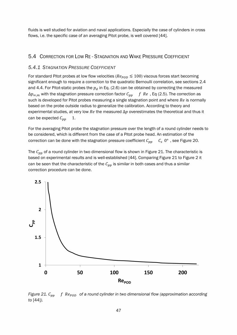
47

fluids is well studied for aviation and naval applications. Especially the case of cylinders in cross flows, i.e. the specific case of an averaging Pitot probe, is well covered [44].

5.4 CORRECTION FOR LOW RE - STAGNATION AND WAKE PRESSURE COEFFICIENT

5.4.1 STAGNATION PRESSURE COEFFICIENT

For standard Pitot probes at low flow velocities (𝑅𝑅𝑅𝑅𝑃𝑃𝑃𝑃𝑃𝑃 ≲ 100) viscous forces start becoming significant enough to require a correction to the quadratic Bernoulli correlation, see sections 2.4 and 4.4. For Pitot-static probes the 𝑝𝑝𝑑𝑑 in Eq. (2.6) can be obtained by correcting the measured ∆𝑝𝑝∞,𝑚𝑚 with the stagnation pressure correction factor 𝐶𝐶𝑝𝑝𝑝𝑝 = 𝑓𝑓(𝑅𝑅𝑅𝑅), Eq (2.5). The correction as such is developed for Pitot probes measuring a single stagnation point and where 𝑅𝑅𝑅𝑅 is normally based on the probe outside radius to generalize the calibration. According to theory and experimental studies, at very low 𝑅𝑅𝑅𝑅 the measured Δ𝑝𝑝 overestimates the theoretical and thus it can be expected 𝐶𝐶𝑝𝑝𝑝𝑝 > 1.

For the averaging Pitot probe the stagnation pressure over the length of a round cylinder needs to be considered, which is different from the case of a Pitot probe head. An estimation of the correction can be done with the stagnation pressure coefficient 𝐶𝐶𝑝𝑝𝑝𝑝 = 𝐶𝐶𝑠𝑠(0°), see Figure 20.

The 𝐶𝐶𝑝𝑝𝑝𝑝 of a round cylinder in two dimensional flow is shown in Figure 21. The characteristic is based on experimental results and is well-established [44]. Comparing Figure 21 to Figure 2 it can be seen that the characteristic of the 𝐶𝐶𝑝𝑝𝑝𝑝 is similar in both cases and thus a similar correction procedure can be done.

Figure 21. 𝐶𝐶𝑝𝑝𝑝𝑝 = 𝑓𝑓(𝑅𝑅𝑅𝑅𝑃𝑃𝑃𝑃𝑃𝑃) of a round cylinder in two dimensional flow (approximation according to [44]).

1

1.5

2

2.5

0 50 100 150 200

C pp

RePOD

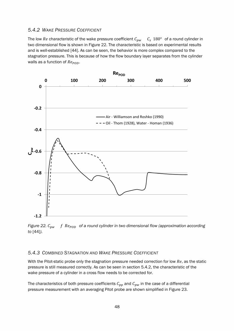
48

5.4.2 WAKE PRESSURE COEFFICIENT

The low 𝑅𝑅𝑅𝑅 characteristic of the wake pressure coefficient 𝐶𝐶𝑝𝑝𝑝𝑝 = 𝐶𝐶𝑠𝑠(180°) of a round cylinder in two dimensional flow is shown in Figure 22. The characteristic is based on experimental results and is well-established [44]. As can be seen, the behavior is more complex compared to the stagnation pressure. This is because of how the flow boundary layer separates from the cylinder walls as a function of 𝑅𝑅𝑅𝑅𝑃𝑃𝑃𝑃𝑃𝑃.

Figure 22. 𝐶𝐶𝑝𝑝𝑝𝑝 = 𝑓𝑓(𝑅𝑅𝑅𝑅𝑃𝑃𝑃𝑃𝑃𝑃) of a round cylinder in two dimensional flow (approximation according to [44]).

5.4.3 COMBINED STAGNATION AND WAKE PRESSURE COEFFICIENT

With the Pitot-static probe only the stagnation pressure needed correction for low 𝑅𝑅𝑅𝑅, as the static pressure is still measured correctly. As can be seen in section 5.4.2, the characteristic of the wake pressure of a cylinder in a cross flow needs to be corrected for.

The characteristics of both pressure coefficients 𝐶𝐶𝑝𝑝𝑝𝑝 and 𝐶𝐶𝑝𝑝𝑝𝑝 in the case of a differential pressure measurement with an averaging Pitot probe are shown simplified in Figure 23.

-1.2

-1

-0.8

-0.6

-0.4

-0.2

00 100 200 300 400 500

C pw

RePOD

Air - Williamson and Roshko (1990)Oil - Thom (1928), Water - Homan (1936)

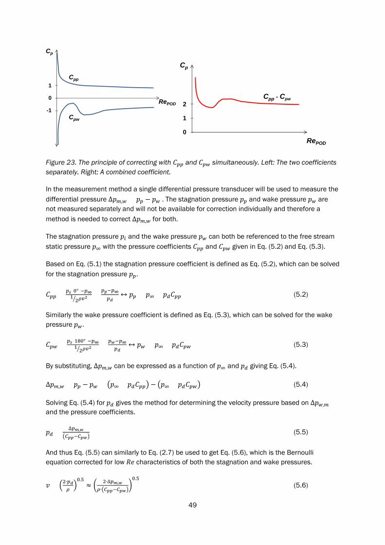
49

Figure 23. The principle of correcting with 𝐶𝐶𝑝𝑝𝑝𝑝 and 𝐶𝐶𝑝𝑝𝑝𝑝 simultaneously. Left: The two coefficients separately. Right: A combined coefficient.

In the measurement method a single differential pressure transducer will be used to measure the differential pressure ∆𝑝𝑝𝑚𝑚,𝑝𝑝 = 𝑝𝑝𝑝𝑝 − 𝑝𝑝𝑝𝑝 . The stagnation pressure 𝑝𝑝𝑝𝑝 and wake pressure 𝑝𝑝𝑝𝑝 are not measured separately and will not be available for correction individually and therefore a method is needed to correct ∆𝑝𝑝𝑚𝑚,𝑝𝑝 for both.

The stagnation pressure 𝑝𝑝𝑖𝑖 and the wake pressure 𝑝𝑝𝑝𝑝 can both be referenced to the free stream static pressure 𝑝𝑝∞ with the pressure coefficients 𝐶𝐶𝑝𝑝𝑝𝑝 and 𝐶𝐶𝑝𝑝𝑝𝑝 given in Eq. (5.2) and Eq. (5.3).

Based on Eq. (5.1) the stagnation pressure coefficient is defined as Eq. (5.2), which can be solved for the stagnation pressure 𝑝𝑝𝑝𝑝.

𝐶𝐶𝑝𝑝𝑝𝑝 = 𝑝𝑝𝑠𝑠(0°)−𝑝𝑝∞12� 𝜌𝜌𝜌𝜌2

= 𝑝𝑝𝑝𝑝−𝑝𝑝∞𝑝𝑝𝑑𝑑

↔ 𝑝𝑝𝑝𝑝 = 𝑝𝑝∞ + 𝑝𝑝𝑑𝑑𝐶𝐶𝑝𝑝𝑝𝑝 (5.2)

Similarly the wake pressure coefficient is defined as Eq. (5.3), which can be solved for the wake pressure 𝑝𝑝𝑝𝑝.

𝐶𝐶𝑝𝑝𝑝𝑝 = 𝑝𝑝𝑠𝑠(180°)−𝑝𝑝∞12� 𝜌𝜌𝜌𝜌2

= 𝑝𝑝𝑤𝑤−𝑝𝑝∞𝑝𝑝𝑑𝑑

↔ 𝑝𝑝𝑝𝑝 = 𝑝𝑝∞ + 𝑝𝑝𝑑𝑑𝐶𝐶𝑝𝑝𝑝𝑝 (5.3)

By substituting, ∆𝑝𝑝𝑚𝑚,𝑝𝑝 can be expressed as a function of 𝑝𝑝∞ and 𝑝𝑝𝑑𝑑 giving Eq. (5.4).

∆𝑝𝑝𝑚𝑚,𝑝𝑝 = 𝑝𝑝𝑝𝑝 − 𝑝𝑝𝑝𝑝 = �𝑝𝑝∞ + 𝑝𝑝𝑑𝑑𝐶𝐶𝑝𝑝𝑝𝑝� − �𝑝𝑝∞ + 𝑝𝑝𝑑𝑑𝐶𝐶𝑝𝑝𝑝𝑝� (5.4)

Solving Eq. (5.4) for 𝑝𝑝𝑑𝑑 gives the method for determining the velocity pressure based on ∆𝑝𝑝𝑝𝑝,𝑚𝑚 and the pressure coefficients.

𝑝𝑝𝑑𝑑 = ∆𝑝𝑝𝑚𝑚,𝑤𝑤�𝐶𝐶𝑝𝑝𝑝𝑝−𝐶𝐶𝑝𝑝𝑤𝑤�

(5.5)

And thus Eq. (5.5) can similarly to Eq. (2.7) be used to get Eq. (5.6), which is the Bernoulli equation corrected for low 𝑅𝑅𝑅𝑅 characteristics of both the stagnation and wake pressures.

𝑣𝑣 = �2∙𝑝𝑝𝑑𝑑𝜌𝜌�0.5

≈ � 2∙∆𝑝𝑝𝑚𝑚,𝑤𝑤𝜌𝜌∙�𝐶𝐶𝑝𝑝𝑝𝑝−𝐶𝐶𝑝𝑝𝑤𝑤�

�0.5

(5.6)

Cpp

Cpw

Cp

1

0

-1

--

--

--

RePODCpp - Cpw

Cp

2

1

0

--

--

--

RePOD

50

While 𝐶𝐶𝑝𝑝𝑝𝑝 and 𝐶𝐶𝑝𝑝𝑝𝑝 cannot be determined separately by a single differential pressure measurement, using Eq. (5.6) it should be possible to calibrate the probe by using a combined correction �𝐶𝐶𝑝𝑝𝑝𝑝 − 𝐶𝐶𝑝𝑝𝑝𝑝�, see also Figure 23, applied to the measured differential pressure ∆𝑝𝑝𝑚𝑚,𝑝𝑝.

As a conclusion it can be said, that similarly to the Pitot-static probe, a low 𝑅𝑅𝑅𝑅 correction should be possible to calibrate the averaging pitot probe for the flow velocities present in residential chimneys.

Note that for the averaging probe a 𝑅𝑅𝑅𝑅𝑃𝑃𝑃𝑃𝑃𝑃 based on the average flow velocity in the duct is needed, and thus in the following analysis there is the assumption that the average 𝑅𝑅𝑅𝑅𝑃𝑃𝑃𝑃𝑃𝑃 of a velocity profile in a duct results in corresponding average 𝐶𝐶𝑝𝑝𝑝𝑝 and 𝐶𝐶𝑝𝑝𝑝𝑝. The theoretically correct way would be to integrate 𝑅𝑅𝑅𝑅𝑃𝑃𝑃𝑃𝑃𝑃 over the length of the probe (i.e. the duct diameter) considering the velocity profile, see section 4.3. However, the velocity profile is not known and is also varying during the measurements, and thus a simpler approach is needed.

It should also be noted that Figures 21 and 22 probably do not apply as such for situations with close proximity to walls, as they are based on measurements without end plates, i.e. a cylinder with no obstructions attached to the ends. The literature implies that especially the behavior of the wake, and thus the characteristic of the 𝐶𝐶𝑝𝑝𝑝𝑝, will change with the presence of end plates [45].

51

6 PROTOTYPE AVERAGING PITOT PROBE

Two chimney-probe combinations were constructed, in this text denoted D80 and D100, with the inner diameters of the ducts 𝐷𝐷𝑖𝑖 = 80.5mm and 𝐷𝐷𝑖𝑖 = 104.5mm, respectively. Stainless steel pipe is used as duct material and the chimneys are insulated according to normal procedure with fire proof mineral/glass wool.

The probe and the chimney were constructed and calibrated as a combination (see Figure 29), i.e. the probes were not intended to be used in other ducts. A straight duct of approximately 6 ×𝐷𝐷𝑖𝑖 length, a 90° bend, followed by another 6 × 𝐷𝐷𝑖𝑖 of straight duct before the averaging pressure probe, are a fixed part of the chimney construction as an attempt to insure a somewhat similar velocity profile when different boilers are connected to it with a flexible duct of stainless steel in the laboratory.

For the prototype probes a very simple design was chosen using two parallel tubes, one as impact pressure chamber and the other as wake pressure chamber, see Figure 24 and 25. Two pipe connectors were attached to the duct wall in a 90° angle with respect to each other for inserting the probes for the two crossing diameters. The design was chosen because of the easy construction allowing adaptation to desired ducts and manufacturing in a local workshop, if changes would be necessary.

Each probe was made of two parallel copper tubes (outer diameter 𝑑𝑑𝑝𝑝𝑝𝑝 = 6mm, wall thickness 1.0 mm). Standard copper tube was chosen as material for the prototypes because of easy access to standard pipe parts and easy manufacturing with standard workshop equipment. Because of lower heat conductivity stainless steel would be a better material for a final product.

Impact pressure ports were drilled on the tube facing the flow and wake pressure ports on the tube facing downstream. The holes are of 2 mm diameter and were spaced according to the “log-linear” velocity area method (3 points per radius, without a center port) [14], [15], with the same spacing for both impact and wake pressures. Pressure port number, placing and size optimizations were left out of scope at this stage and thus there may be a possibility for further optimization for the intended application, see section 5.1.

The probe is equipped with a standard copper tube clamp ring connector, so that it can be attached to the duct connector thread. The construction is such that the probe can be removed for cleaning in a few seconds, also while the boiler is in operation, and the probe always locks to the same position when inserted so that the alignment with flow does not change.

To ensure a representative average bulk temperature three thermocouple sensors are used, Figure 24 and 25. The temperature sensors are placed close to the flow sensor, forming a triangle in the duct cross section. Each temperature is logged separately and averaged arithmetically afterwards in the data processing. The temperature sensors are placed 50mm downstream from the averaging pressure probe and a guiding fitting was made to the threaded duct connection so that the temperature sensors can be easily pulled out or changed.

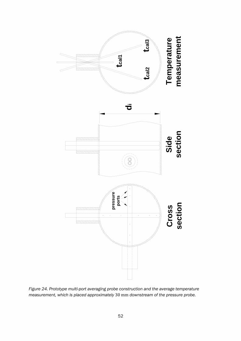
52

Figure 24. Prototype multi-port averaging probe construction and the average temperature measurement, which is placed approximately 30 mm downstream of the pressure probe.

Cro

ssse

ctio

nSi

dese

ctio

n

di

pres

sure

port

s

Tem

pera

ture

mea

sure

men

t

tcal1

tcal2

tcal3

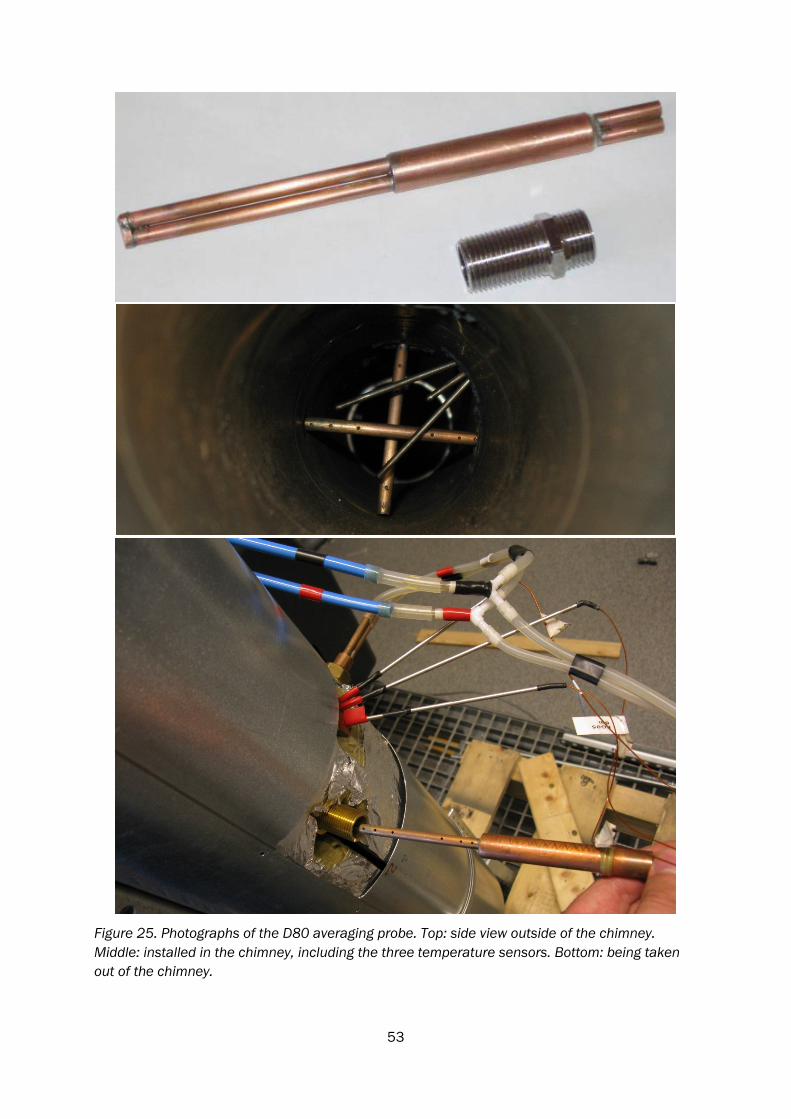
53

Figure 25. Photographs of the D80 averaging probe. Top: side view outside of the chimney. Middle: installed in the chimney, including the three temperature sensors. Bottom: being taken out of the chimney.

54

7 DIFFERENTIAL PRESSURE TRANSDUCERS

The low differential pressures generated in averaging and Pitot-static probes in the considered application present a difficult challenge of finding a transducer with acceptable performance. Some considerations regarding their performance are explored and the results of testing three different transducers are presented here.

7.1 BACKGROUND The aim was to use off-the-shelf industry standard pressure transducers. Such pressure transducers are not calibrated for measuring the low differential pressures in the application described here, see section 4.11. Even if the considered transducers can give a useable signal, the problem is that direct calibration for ∆𝑝𝑝𝑚𝑚 < 1 Pa is not readily available as the standard calibration in laboratories has an uncertainty of ±0.2 Pa.

However, as a flow measurement can be calibrated directly by correlating the output signal to a known flow rate, as described in section 8, the transducers can be still be used ignoring the calibration of the pressure reading. Care still has to be taken in the choice of the transducer so that the performance fits the needs of the application.

Pressure transducers based on both digital (DSP) and analogue (ASP) signal processing can be found on the market. In the DSP version the signal can be digitally processed various ways (re-scaling, averaging, unit conversions, corrections for ambient conditions, etc.) before it is converted and passed on as an industry standard electrical current or voltage signal. In the ASP version the signal is conditioned, amplified and converted to an industry standard signal. The most significant difference is that DSP requires analog to digital signal conversion (ADC) before DSP and digital to analog conversion (DAC) after. Due to the complex nature of differential pressures produced by gas flow measurements DSP is normally preferred over ASP because of the possibility for complex signal processing functions, but also has limitations regarding resolution, mainly in the ADC.

Care has to be taken in the choice of the transducer, as with DSP the range and resolution of the first ADC is crucial as the analog signal conditioning before it is normally fixed in the circuit design of a commercial product. How the measurement range is adapted to the ADC defines the absolute resolution of the measurement and thus the lowest flow rate that can be measured, and its uncertainty. The signal output (the DAC after the DSP) does not seem to be an issue, and in some devices it can also be re-scaled by the user

7.2 EXPERIMENTAL COMPARISON OF PRESSURE TRANSDUCERS Three different transducers, PT1, PT2 and PT3, were tested at low flow rates. PT1 is a late 90’s transducer with onboard DSP doing only averaging, range 0 Pa to 50 Pa. PT2 is a model manufactured in 2007, where the onboard DSP can be used for several signal processing functions, range 0 Pa to 100 Pa. PT3 is a simpler model from 2007, but specifically designed for

55

relatively low differential pressures and equipped with automatic zero level adjustment, range 0 Pa to 10 Pa.

A pressure transducer utilizing purely ASP was not found, although there seem to be OEM (Original Equipment Manufacturer) pressure gauges available. Using an OEM gauge would also require choosing (or designing and constructing) an appropriate amplification and conditioning circuit.

7.2.1 MEASUREMENT SETUP

The tests were performed with the D80 averaging pitot probe prototype described in section 6 and the calibration rig described in section 8.1. The purpose was to find out how the transducers perform in producing the output voltage signal 𝑈𝑈𝑐𝑐𝑙𝑙𝑙𝑙 in the intended operating range of the averaging Pitot probe. The tests were performed running the system at different constant flow rates logging with a 10 s sampling interval of the output signal of the parallel connected transducers.

Figures 26 through 28 show the results, the bottom figures are zoomed in on the dashed box in the upper figures. The y-axis scaling is different in each case because the signal outputs of the transducers differ. The spread of the samples in the y-axis direction during the steady states is due to transducer performance. The spread in the x-axis direction comes from the reference flow measurement and is due to the flow rate not being completely constant.

7.2.2 RESOLUTION AND STABILITY

PT2 and PT3 are clearly not suitable for the range 0 m/s to 0.4 m/s. PT2 has a kink in its response (at ~0.18 m/s), the cause of which could not be determined. PT3 shows the impact of automatic zero level adjustment (at ~0.2 m/s) where the signal is reset corresponding to a new zero differential pressure level. PT2 and PT3 show also insufficient ADC resolution for the range 0 m/s to 0.4 m/s, which can be seen as y-axis spread and graininess of the samples.

The y-axis spread of the samples with PT2 and PT3 can be due to unstable sensor or insufficient averaging time constant, but can also be the result of insufficient ADC resolution. From around 0.4 m/s onwards both PT2 and PT3 would have sufficient correlation to the flow rate for measurement. As PT1 gave apparently the best performance for low flow rates it was chosen for further testing.

7.2.3 TEMPERATURE DRIFT

The temperature drift of the signal output can be significant regarding the lowest flow rates. Some manufacturers have automatic corrections for the ambient temperature built in the electronics.

As an example, for PT1 the specified temperature drift is <0.5 % of the range per 10 °C corresponding to 0.025 Pa/°C. From Figure 15 in can be read that the average expected differential pressures are approximately 5 Pa for nominal and 1.5 Pa for 30 % combustion power.

56

For these differential pressures the temperature drift of 0.025 Pa/°C translates to an uncertainty of ±0.5 % and ±1.6 %, respectively, for a ±1 °C ambient temperature change.

The easiest remedy is to keep the ambient temperature of the device as constant as possible. Otherwise the temperature drift should be measured, modeled and corrected for. This, however, is a very time consuming procedure, as it requires the calibration curves to be done at several ambient temperatures and also a time constant should be determined for the stabilization. Measurements and modeling of the temperature drift was considered and tested, but was left out of scope for this work.

7.2.4 HYSTERESIS, NOISE, TIME CONSTANT

Hysteresis may appear in pressure transducers as slightly different results for rising and falling differential pressures. Another form of hysteresis is “sticky values”, where the signal output appears to change in steps, or not settle back to an initial value. These are often also time dependent and may thus be difficult to differentiate from the time constant of the averaging function, which is explained next.

The signal outputs of pressure measurements in gas flows are inherently relatively noisy, requiring both filtering and averaging. The averaging (also sometimes called damping) is done over a period of time in the order of milliseconds to tens of seconds, depending on the objective of the measurement. This averaging time is often called Time constant in manufacturer specification sheets.

It should be noted that the time constant of the averaging function is different from settling times due to hysteresis, viscous forces, and internal gas volumes of the membrane and the tube passages, see section 4.4.2. Each of these phenomena contribute to an overall time constant of the measurement.

Hysteresis, time constant and noise were left out of scope of this study as initial testing did not give apparent indications of these being an issue.

7.2.5 ZERO LEVEL ADJUSTMENT - AUTOMATIC ZEROING The signal output of a transducer at zero differential pressure is not constant. There is an offset, which is changing because the membrane and surrounding electronics are exposed to several ambient effects, mainly temperature. For the intended normal industrial applications of the transducers, these effects are usually negligible, but for the application discussed in this work they may be significant.

The zero differential pressure signal level should thus be checked and logged regularly. In this work an arrangement of 3-way valves was constructed to the pressure passages so that the transducer high and low pressure inlets can easily be exposed to the same pressure in a chamber protected from ambient air movement disturbances. Zero levels were normally logged as a steady state average of 3 minutes.

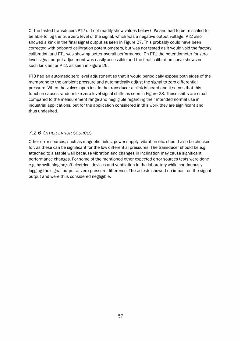
57

Of the tested transducers PT2 did not readily show values below 0 Pa and had to be re-scaled to be able to log the true zero level of the signal, which was a negative output voltage. PT2 also showed a kink in the final signal output as seen in Figure 27. This probably could have been corrected with onboard calibration potentiometers, but was not tested as it would void the factory calibration and PT1 was showing better overall performance. On PT1 the potentiometer for zero level signal output adjustment was easily accessible and the final calibration curve shows no such kink as for PT2, as seen in Figure 26.

PT3 had an automatic zero level adjustment so that it would periodically expose both sides of the membrane to the ambient pressure and automatically adjust the signal to zero differential pressure. When the valves open inside the transducer a click is heard and it seems that this function causes random-like zero level signal shifts as seen in Figure 28. These shifts are small compared to the measurement range and negligible regarding their intended normal use in industrial applications, but for the application considered in this work they are significant and thus undesired.

7.2.6 OTHER ERROR SOURCES

Other error sources, such as magnetic fields, power supply, vibration etc. should also be checked for, as these can be significant for the low differential pressures. The transducer should be e.g. attached to a stable wall because vibration and changes in inclination may cause significant performance changes. For some of the mentioned other expected error sources tests were done e.g. by switching on/off electrical devices and ventilation in the laboratory while continuously logging the signal output at zero pressure difference. These tests showed no impact on the signal output and were thus considered negligible.

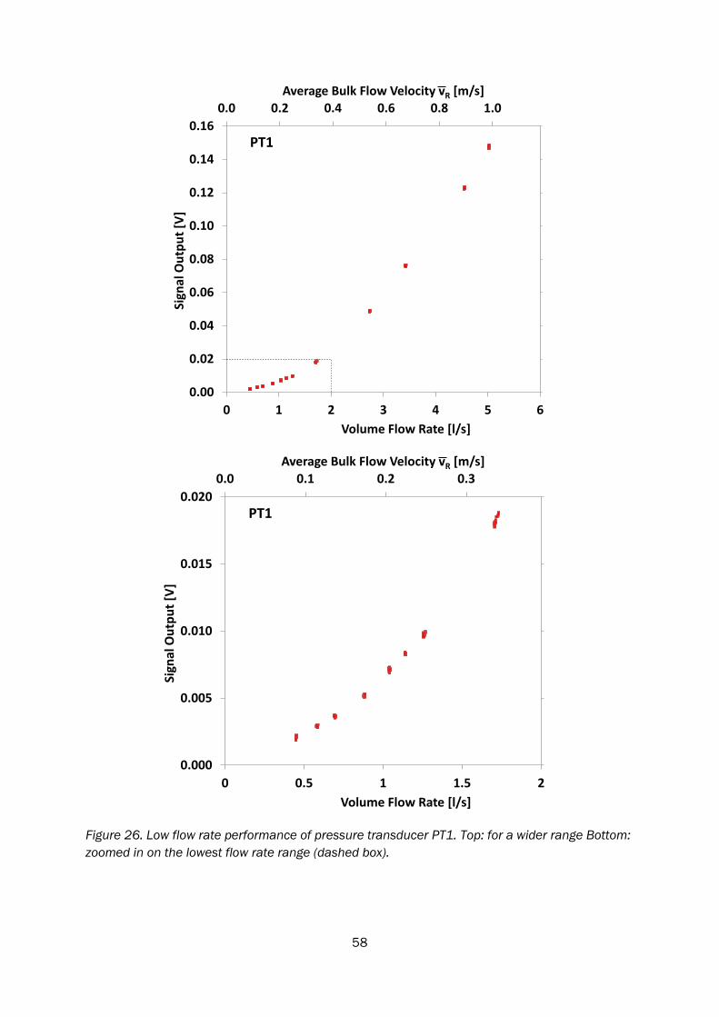
58

Figure 26. Low flow rate performance of pressure transducer PT1. Top: for a wider range Bottom: zoomed in on the lowest flow rate range (dashed box).

0.0 0.2 0.4 0.6 0.8 1.0

0.00

0.02

0.04

0.06

0.08

0.10

0.12

0.14

0.16

0 1 2 3 4 5 6

Average Bulk Flow Velocity vR [m/s]

Sign

al O

utpu

t [V]

Volume Flow Rate [l/s]

PT1

0.0 0.1 0.2 0.3

0.000

0.005

0.010

0.015

0.020

0 0.5 1 1.5 2

Average Bulk Flow Velocity vR [m/s]

Sign

al O

utpu

t [V]

Volume Flow Rate [l/s]

PT1

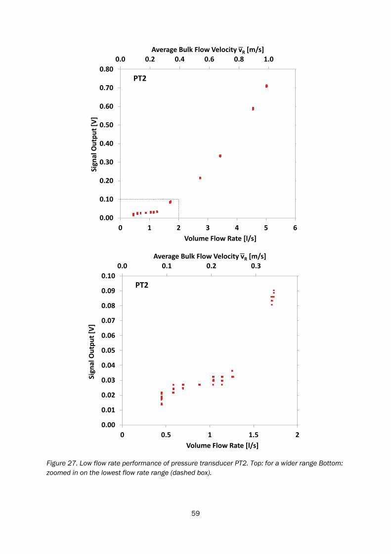
59

Figure 27. Low flow rate performance of pressure transducer PT2. Top: for a wider range Bottom: zoomed in on the lowest flow rate range (dashed box).

0.0 0.2 0.4 0.6 0.8 1.0

0.00

0.10

0.20

0.30

0.40

0.50

0.60

0.70

0.80

0 1 2 3 4 5 6

Average Bulk Flow Velocity vR [m/s]

Sign

al O

utpu

t [V]

Volume Flow Rate [l/s]

PT2

0.0 0.1 0.2 0.3

0.00

0.01

0.02

0.03

0.04

0.05

0.06

0.07

0.08

0.09

0.10

0 0.5 1 1.5 2

Average Bulk Flow Velocity vR [m/s]

Sign

al O

utpu

t [V]

Volume Flow Rate [l/s]

PT2

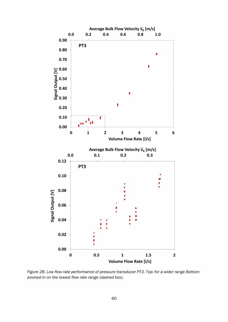
60

Figure 28. Low flow rate performance of pressure transducer PT3. Top: for a wider range Bottom: zoomed in on the lowest flow rate range (dashed box).

0.0 0.2 0.4 0.6 0.8 1.0

0.00

0.10

0.20

0.30

0.40

0.50

0.60

0.70

0.80

0.90

0 1 2 3 4 5 6

Average Bulk Flow Velocity vR [m/s]

Sign

al O

utpu

t [V]

Volume Flow Rate [l/s]

PT3

0.0 0.1 0.2 0.3

0.00

0.02

0.04

0.06

0.08

0.10

0.12

0 0.5 1 1.5 2

Average Bulk Flow Velocity vR [m/s]

Sign

al O

utpu

t [V]

Volume Flow Rate [l/s]

PT3

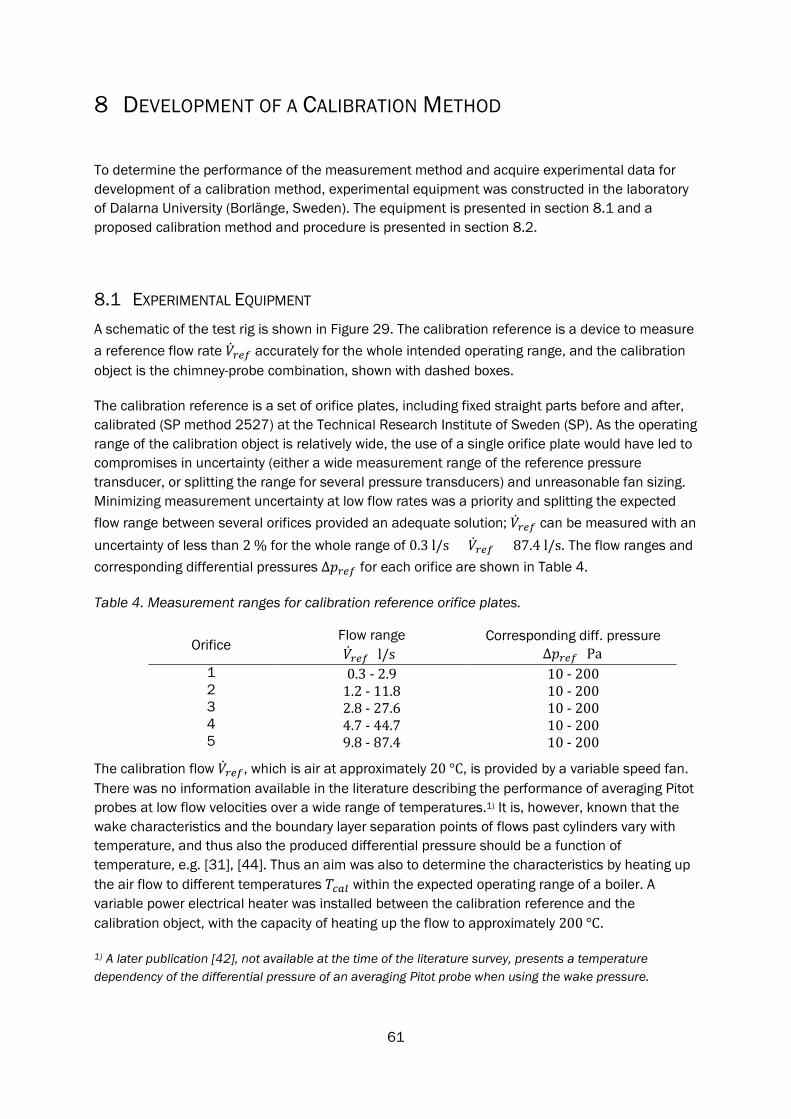
61

8 DEVELOPMENT OF A CALIBRATION METHOD

To determine the performance of the measurement method and acquire experimental data for development of a calibration method, experimental equipment was constructed in the laboratory of Dalarna University (Borlänge, Sweden). The equipment is presented in section 8.1 and a proposed calibration method and procedure is presented in section 8.2.

8.1 EXPERIMENTAL EQUIPMENT A schematic of the test rig is shown in Figure 29. The calibration reference is a device to measure a reference flow rate �̇�𝑉𝑐𝑐𝑅𝑅𝑓𝑓 accurately for the whole intended operating range, and the calibration object is the chimney-probe combination, shown with dashed boxes.

The calibration reference is a set of orifice plates, including fixed straight parts before and after, calibrated (SP method 2527) at the Technical Research Institute of Sweden (SP). As the operating range of the calibration object is relatively wide, the use of a single orifice plate would have led to compromises in uncertainty (either a wide measurement range of the reference pressure transducer, or splitting the range for several pressure transducers) and unreasonable fan sizing. Minimizing measurement uncertainty at low flow rates was a priority and splitting the expected flow range between several orifices provided an adequate solution; �̇�𝑉𝑐𝑐𝑅𝑅𝑓𝑓 can be measured with an uncertainty of less than 2 % for the whole range of 0.3 l/s < �̇�𝑉𝑐𝑐𝑅𝑅𝑓𝑓 < 87.4 l/s. The flow ranges and corresponding differential pressures ∆𝑝𝑝𝑐𝑐𝑅𝑅𝑓𝑓 for each orifice are shown in Table 4.

Table 4. Measurement ranges for calibration reference orifice plates.

Orifice Flow range �̇�𝑉𝑐𝑐𝑅𝑅𝑓𝑓 [l/s]

Corresponding diff. pressure ∆𝑝𝑝𝑐𝑐𝑅𝑅𝑓𝑓 [Pa]

1 0.3 - 2.9 10 - 200 2 1.2 - 11.8 10 - 200 3 2.8 - 27.6 10 - 200 4 4.7 - 44.7 10 - 200 5 9.8 - 87.4 10 - 200

The calibration flow �̇�𝑉𝑐𝑐𝑅𝑅𝑓𝑓, which is air at approximately 20 °C, is provided by a variable speed fan. There was no information available in the literature describing the performance of averaging Pitot probes at low flow velocities over a wide range of temperatures.1) It is, however, known that the wake characteristics and the boundary layer separation points of flows past cylinders vary with temperature, and thus also the produced differential pressure should be a function of temperature, e.g. [31], [44]. Thus an aim was also to determine the characteristics by heating up the air flow to different temperatures 𝑇𝑇𝑐𝑐𝑙𝑙𝑙𝑙 within the expected operating range of a boiler. A variable power electrical heater was installed between the calibration reference and the calibration object, with the capacity of heating up the flow to approximately 200 °C.

1) A later publication [42], not available at the time of the literature survey, presents a temperature dependency of the differential pressure of an averaging Pitot probe when using the wake pressure.

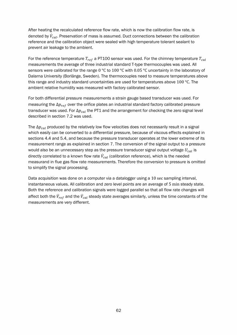
62

After heating the recalculated reference flow rate, which is now the calibration flow rate, is denoted by �̇�𝑉𝑐𝑐𝑙𝑙𝑙𝑙. Preservation of mass is assumed. Duct connections between the calibration reference and the calibration object were sealed with high temperature tolerant sealant to prevent air leakage to the ambient.

For the reference temperature 𝑇𝑇𝑐𝑐𝑅𝑅𝑓𝑓 a PT100 sensor was used. For the chimney temperature 𝑇𝑇𝑐𝑐𝑙𝑙𝑙𝑙 measurements the average of three industrial standard T-type thermocouples was used. All sensors were calibrated for the range 0 °C to 100 °C with 0.05 °C uncertainty in the laboratory of Dalarna University (Borlänge, Sweden). The thermocouples need to measure temperatures above this range and industry standard uncertainties are used for temperatures above 100 °C. The ambient relative humidity was measured with factory calibrated sensor.

For both differential pressure measurements a strain gauge based transducer was used. For measuring the ∆𝑝𝑝𝑐𝑐𝑅𝑅𝑓𝑓 over the orifice plates an industrial standard factory calibrated pressure transducer was used. For ∆𝑝𝑝𝑐𝑐𝑙𝑙𝑙𝑙 the PT1 and the arrangement for checking the zero signal level described in section 7.2 was used.

The ∆𝑝𝑝𝑐𝑐𝑙𝑙𝑙𝑙 produced by the relatively low flow velocities does not necessarily result in a signal which easily can be converted to a differential pressure, because of viscous effects explained in sections 4.4 and 5.4, and because the pressure transducer operates at the lower extreme of its measurement range as explained in section 7. The conversion of the signal output to a pressure would also be an unnecessary step as the pressure transducer signal output voltage 𝑈𝑈𝑐𝑐𝑙𝑙𝑙𝑙 is directly correlated to a known flow rate �̇�𝑉𝑐𝑐𝑙𝑙𝑙𝑙 (calibration reference), which is the needed measurand in flue gas flow rate measurements. Therefore the conversion to pressure is omitted to simplify the signal processing.

Data acquisition was done on a computer via a datalogger using a 10 sec sampling interval, instantaneous values. All calibration and zero level points are an average of 5 min steady state. Both the reference and calibration signals were logged parallel so that all flow rate changes will affect both the �̇�𝑉𝑐𝑐𝑅𝑅𝑓𝑓 and the �̇�𝑉𝑐𝑐𝑙𝑙𝑙𝑙 steady state averages similarly, unless the time constants of the measurements are very different.

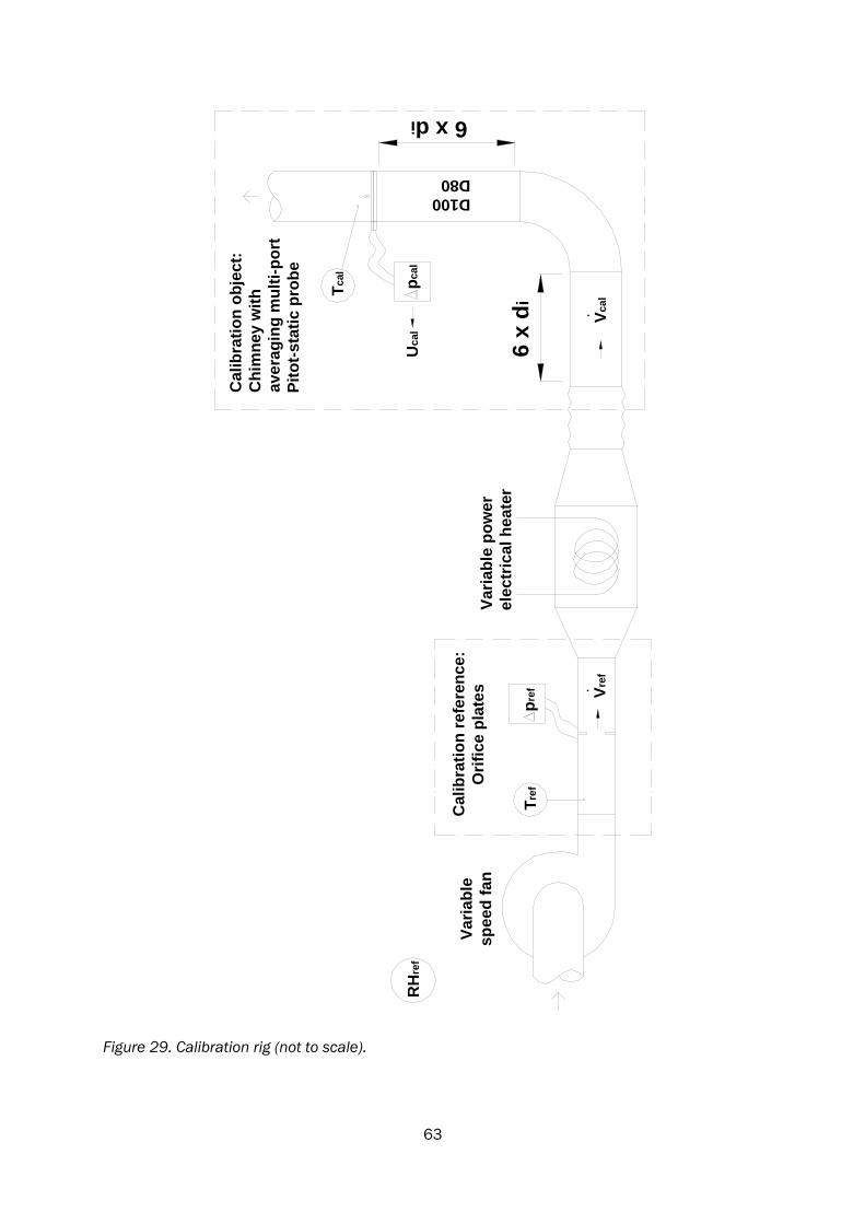
63

Figure 29. Calibration rig (not to scale).

Orif

ice

plat

es ra

nges

(Cal

ibra

ted

at S

P)

Varia

ble

spee

d fa

n

1. 0

.3-2

.9 l

/s =

10-

200

Pa2.

1.2

-11.

8 l/s

= 1

0-20

0 Pa

3. 2

.8-2

7.6

l/s =

10-

200

Pa4.

4.7

-44.

7 l/s

= 1

0-20

0 Pa

5. 9

.4-8

7.4

l/s =

10-

200

Pa

Cal

ibra

tion

refe

renc

e:O

rific

e pl

ates

Cal

ibra

tion

obje

ct:

Chi

mne

y w

ith

aver

agin

g m

ulti-

port

Pi

tot-s

tatic

pro

be

Varia

ble

pow

erel

ectr

ical

hea

ter

D100D80

pcal

6 x di

6 x

dipr

efTr

ef

Tcal

RH

ref

. Vref

. Vcal

Uca

l

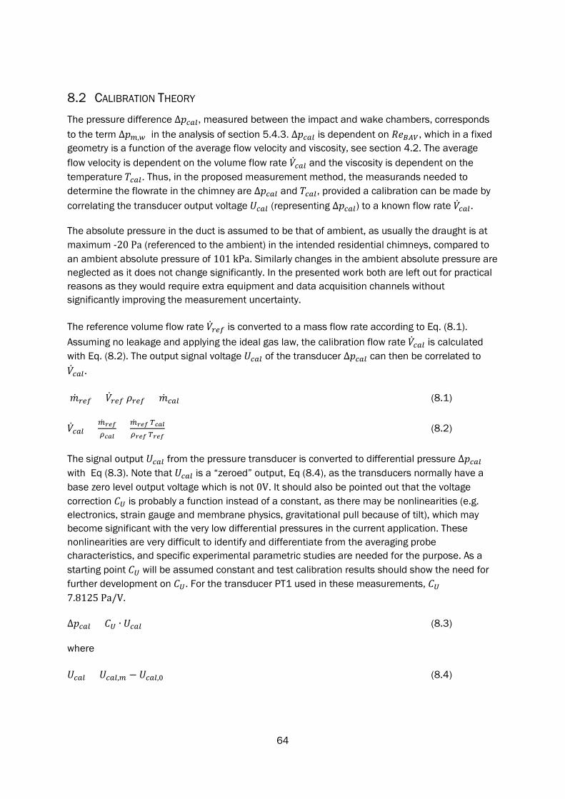
64

8.2 CALIBRATION THEORY The pressure difference ∆𝑝𝑝𝑐𝑐𝑙𝑙𝑙𝑙, measured between the impact and wake chambers, corresponds to the term ∆𝑝𝑝𝑚𝑚,𝑝𝑝 in the analysis of section 5.4.3. ∆𝑝𝑝𝑐𝑐𝑙𝑙𝑙𝑙 is dependent on 𝑅𝑅𝑅𝑅𝐵𝐵𝐵𝐵𝐵𝐵, which in a fixed geometry is a function of the average flow velocity and viscosity, see section 4.2. The average flow velocity is dependent on the volume flow rate �̇�𝑉𝑐𝑐𝑙𝑙𝑙𝑙 and the viscosity is dependent on the temperature 𝑇𝑇𝑐𝑐𝑙𝑙𝑙𝑙. Thus, in the proposed measurement method, the measurands needed to determine the flowrate in the chimney are ∆𝑝𝑝𝑐𝑐𝑙𝑙𝑙𝑙 and 𝑇𝑇𝑐𝑐𝑙𝑙𝑙𝑙, provided a calibration can be made by correlating the transducer output voltage 𝑈𝑈𝑐𝑐𝑙𝑙𝑙𝑙 (representing ∆𝑝𝑝𝑐𝑐𝑙𝑙𝑙𝑙) to a known flow rate �̇�𝑉𝑐𝑐𝑙𝑙𝑙𝑙.

The absolute pressure in the duct is assumed to be that of ambient, as usually the draught is at maximum -20 Pa (referenced to the ambient) in the intended residential chimneys, compared to an ambient absolute pressure of 101 kPa. Similarly changes in the ambient absolute pressure are neglected as it does not change significantly. In the presented work both are left out for practical reasons as they would require extra equipment and data acquisition channels without significantly improving the measurement uncertainty.

The reference volume flow rate �̇�𝑉𝑐𝑐𝑅𝑅𝑓𝑓 is converted to a mass flow rate according to Eq. (8.1). Assuming no leakage and applying the ideal gas law, the calibration flow rate �̇�𝑉𝑐𝑐𝑙𝑙𝑙𝑙 is calculated with Eq. (8.2). The output signal voltage 𝑈𝑈𝑐𝑐𝑙𝑙𝑙𝑙 of the transducer ∆𝑝𝑝𝑐𝑐𝑙𝑙𝑙𝑙 can then be correlated to �̇�𝑉𝑐𝑐𝑙𝑙𝑙𝑙.

�̇�𝑚𝑐𝑐𝑅𝑅𝑓𝑓 = �̇�𝑉𝑐𝑐𝑅𝑅𝑓𝑓 𝜌𝜌𝑐𝑐𝑅𝑅𝑓𝑓 = �̇�𝑚𝑐𝑐𝑙𝑙𝑙𝑙 (8.1)

�̇�𝑉𝑐𝑐𝑙𝑙𝑙𝑙 = �̇�𝑚𝑟𝑟𝑟𝑟𝑓𝑓

𝜌𝜌𝑐𝑐𝑐𝑐𝑐𝑐= �̇�𝑚𝑟𝑟𝑟𝑟𝑓𝑓 𝑇𝑇𝑐𝑐𝑐𝑐𝑐𝑐

𝜌𝜌𝑟𝑟𝑟𝑟𝑓𝑓 𝑇𝑇𝑟𝑟𝑟𝑟𝑓𝑓 (8.2)

The signal output 𝑈𝑈𝑐𝑐𝑙𝑙𝑙𝑙 from the pressure transducer is converted to differential pressure ∆𝑝𝑝𝑐𝑐𝑙𝑙𝑙𝑙 with Eq (8.3). Note that 𝑈𝑈𝑐𝑐𝑙𝑙𝑙𝑙 is a “zeroed” output, Eq (8.4), as the transducers normally have a base zero level output voltage which is not 0V. It should also be pointed out that the voltage correction 𝐶𝐶𝑈𝑈 is probably a function instead of a constant, as there may be nonlinearities (e.g. electronics, strain gauge and membrane physics, gravitational pull because of tilt), which may become significant with the very low differential pressures in the current application. These nonlinearities are very difficult to identify and differentiate from the averaging probe characteristics, and specific experimental parametric studies are needed for the purpose. As a starting point 𝐶𝐶𝑈𝑈 will be assumed constant and test calibration results should show the need for further development on 𝐶𝐶𝑈𝑈. For the transducer PT1 used in these measurements, 𝐶𝐶𝑈𝑈 =7.8125 Pa/V.

∆𝑝𝑝𝑐𝑐𝑙𝑙𝑙𝑙 = 𝐶𝐶𝑈𝑈 ∙ 𝑈𝑈𝑐𝑐𝑙𝑙𝑙𝑙 (8.3)

where

𝑈𝑈𝑐𝑐𝑙𝑙𝑙𝑙 = 𝑈𝑈𝑐𝑐𝑙𝑙𝑙𝑙,𝑚𝑚 − 𝑈𝑈𝑐𝑐𝑙𝑙𝑙𝑙,0 (8.4)

65

Applying Eq. (8.3) to Eq. (2.2) gives Eq. (8.5). This is Bernoulli equation that is not corrected for low 𝑅𝑅𝑅𝑅𝑃𝑃𝑃𝑃𝑃𝑃.

𝑣𝑣𝑐𝑐𝑙𝑙𝑙𝑙 = �2∙𝑝𝑝𝑑𝑑𝜌𝜌�0.5

= �2∙∆𝑝𝑝𝑐𝑐𝑐𝑐𝑐𝑐𝜌𝜌𝑐𝑐𝑐𝑐𝑐𝑐

�0.5

≈ �2 𝐶𝐶𝑈𝑈𝑈𝑈𝑐𝑐𝑐𝑐𝑐𝑐𝜌𝜌𝑐𝑐𝑐𝑐𝑐𝑐

�0.5

(8.5)

Applying Eq. (8.3) to Eq. (5.6) gives Eq. (8.6), which is the correlation correcting for low 𝑅𝑅𝑅𝑅𝑃𝑃𝑃𝑃𝑃𝑃.

𝑣𝑣𝑐𝑐𝑙𝑙𝑙𝑙 = �2 𝑝𝑝𝑑𝑑𝜌𝜌�0.5

= � 2 ∆𝑝𝑝𝑐𝑐𝑐𝑐𝑐𝑐𝜌𝜌𝑐𝑐𝑐𝑐𝑐𝑐 �𝐶𝐶𝑝𝑝𝑝𝑝−𝐶𝐶𝑝𝑝𝑤𝑤�

�0.5

≈ � 2 𝐶𝐶𝑈𝑈𝑈𝑈𝑐𝑐𝑐𝑐𝑐𝑐𝜌𝜌𝑐𝑐𝑐𝑐𝑐𝑐 �𝐶𝐶𝑝𝑝𝑝𝑝−𝐶𝐶𝑝𝑝𝑤𝑤�

�0.5

(8.6)

The volume flow rates corresponding to Eq. (8.5) and (8.6) are given by Eq. (8.7) and (8.8), respectively where 𝐴𝐴𝑃𝑃 is the duct cross sectional area.

�̇�𝑉𝑐𝑐𝑙𝑙𝑙𝑙′ ≈ 𝐴𝐴𝑃𝑃 �2 𝐶𝐶𝑈𝑈𝑈𝑈𝑐𝑐𝑐𝑐𝑐𝑐𝜌𝜌𝑐𝑐𝑐𝑐𝑐𝑐

�0.5

(8.7)

�̇�𝑉𝑐𝑐𝑙𝑙𝑙𝑙′ ≈ 𝐴𝐴𝑃𝑃 �2 𝐶𝐶𝑈𝑈 𝑈𝑈𝑐𝑐𝑐𝑐𝑐𝑐

𝜌𝜌𝑐𝑐𝑐𝑐𝑐𝑐 �𝐶𝐶𝑝𝑝𝑝𝑝−𝐶𝐶𝑝𝑝𝑤𝑤��0.5

(8.8)

Note that in Eq. (8.5) through (8.8), instead of lumped calibration coefficients, the constants 𝐶𝐶𝑈𝑈, 𝐴𝐴𝑃𝑃 and 20.5 are intentionally kept separate to be able to pedagogically differentiate between the correction factors and evaluate them separately.

66

9 TESTING OF THE CALIBRATION METHOD

A set of measurements were performed in the laboratory of Dalarna University (Borlänge, Sweden) during the years 2008-2010. The aim was to test the concept of using an averaging Pitot probe for measuring the low flow rates present in residential chimneys by experimentally confirming the theory presented in section 5 and the calibration procedure proposed in section 8.2.

9.1 DATA SETS After initial test measurements the data sets summarized in Tables 5 and 6 were used in this study.

The isotherm data sets were measured at different temperatures so that a temperature correction could later be studied, if needed. The 𝑇𝑇𝑐𝑐𝑙𝑙𝑙𝑙 for the isotherms chosen were ambient temperature (approximately 17 °C to 20 °C), 70 °C, 120 °C and 170 °C.

The rest of the data sets were performed to study the impact of various disturbances, e.g. changes in the inlet configuration and clogging after use in flue gas flows. Because of construction work the measurement equipment had to be moved to a new laboratory during the experiments and this is pointed out in Tables 5 and 6 as it turned out that the moving temporarily affected the equipment.

Because of both fire hazard and risk of damage to the calibration rig there was a limitation to the minimum flow rates that could be used with certain temperatures, and thus there are fewer points the higher the 𝑇𝑇𝑐𝑐𝑙𝑙𝑙𝑙 and the lower the �̇�𝑉𝑐𝑐𝑙𝑙𝑙𝑙. For a thorough analysis and calibration this is a deficiency, but regarding the intended application this is not crucial. The temperature of flue gas after the boiler correlates with the combustion power and low flue gas flow rates with high temperatures from a normal residential boiler are unlikely.

Figures 30 and 31 show the calibration data sets D80_7 through D80_10 and D100_7 through D100_10. These isotherms were specifically done to study the temperature dependency of the signal output and the correlations. The dashed curves and lines following the data points are curve fits to aid visualization of the isotherms. 𝑅𝑅𝑅𝑅𝐵𝐵𝐵𝐵𝐵𝐵 is shown for evaluation of the flow type in the duct and 𝑅𝑅𝑅𝑅𝑃𝑃𝑃𝑃𝑃𝑃 for evaluating the viscous forces affecting the measurement. It should be noted that 𝑅𝑅𝑅𝑅𝑃𝑃𝑃𝑃𝑃𝑃 is based on the average flow velocity along the probe length (duct diameter) and cannot directly be compared to values from literature, which are mostly based on measurements with a uniform velocity across the length of the cylinder.

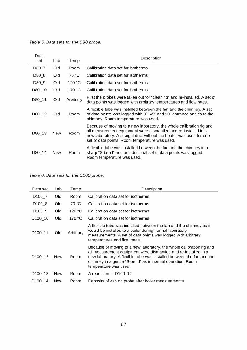
67

Table 5. Data sets for the D80 probe.

Data set Lab Temp Description

D80_7 Old Room Calibration data set for isotherms

D80_8 Old 70 °C Calibration data set for isotherms

D80_9 Old 120 °C Calibration data set for isotherms

D80_10 Old 170 °C Calibration data set for isotherms

D80_11 Old Arbitrary First the probes were taken out for “cleaning” and re-installed. A set of data points was logged with arbitrary temperatures and flow rates.

D80_12 Old Room A flexible tube was installed between the fan and the chimney. A set of data points was logged with 0º, 45º and 90º entrance angles to the chimney. Room temperature was used.

D80_13 New Room

Because of moving to a new laboratory, the whole calibration rig and all measurement equipment were dismantled and re-installed in a new laboratory. A straight duct without the heater was used for one set of data points. Room temperature was used.

D80_14 New Room A flexible tube was installed between the fan and the chimney in a sharp “S-bend” and an additional set of data points was logged. Room temperature was used.

Table 6. Data sets for the D100 probe.

Data set Lab Temp Description

D100_7 Old Room Calibration data set for isotherms

D100_8 Old 70 °C Calibration data set for isotherms

D100_9 Old 120 °C Calibration data set for isotherms

D100_10 Old 170 °C Calibration data set for isotherms

D100_11 Old Arbitrary

A flexible tube was installed between the fan and the chimney as it would be installed to a boiler during normal laboratory measurements. A set of data points was logged with arbitrary temperatures and flow rates.

D100_12 New Room

Because of moving to a new laboratory, the whole calibration rig and all measurement equipment were dismantled and re-installed in a new laboratory. A flexible tube was installed between the fan and the chimney in a gentle “S-bend” as in normal operation. Room temperature was used.

D100_13 New Room A repetition of D100_12

D100_14 New Room Deposits of ash on probe after boiler measurements

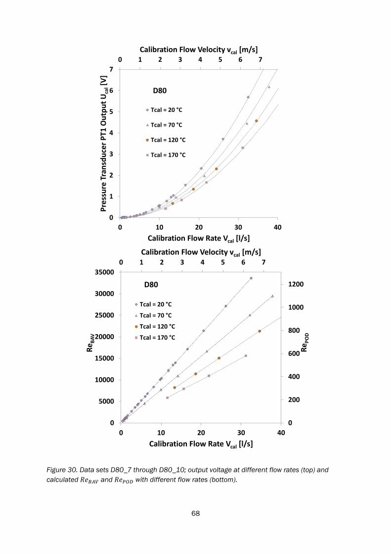
68

Figure 30. Data sets D80_7 through D80_10; output voltage at different flow rates (top) and calculated 𝑅𝑅𝑅𝑅𝐵𝐵𝐵𝐵𝐵𝐵 and 𝑅𝑅𝑅𝑅𝑃𝑃𝑃𝑃𝑃𝑃 with different flow rates (bottom).

0 1 2 3 4 5 6 7

0

1

2

3

4

5

6

7

0 10 20 30 40

Calibration Flow Velocity vcal [m/s]

Pres

sure

Tra

nsdu

cer P

T1 O

utpu

t Uca

l[V]

Calibration Flow Rate Vcal [l/s]

Tcal = 20 °C

Tcal = 70 °C

Tcal = 120 °C

Tcal = 170 °C

D80

0

200

400

600

800

1000

1200

0 1 2 3 4 5 6 7

0

5000

10000

15000

20000

25000

30000

35000

0 10 20 30 40

RePO

D

Calibration Flow Velocity vcal [m/s]

ReBA

V

Calibration Flow Rate Vcal [l/s]

Tcal = 20 °C

Tcal = 70 °C

Tcal = 120 °C

Tcal = 170 °C

D80

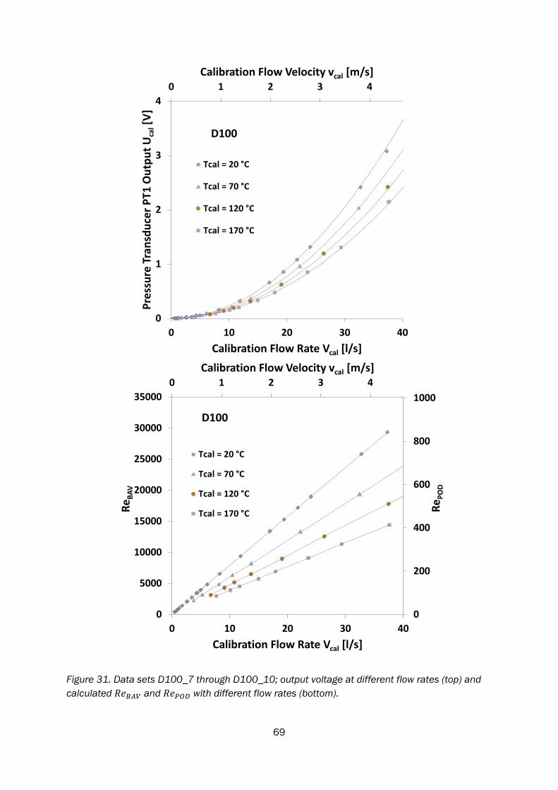
69

Figure 31. Data sets D100_7 through D100_10; output voltage at different flow rates (top) and calculated 𝑅𝑅𝑅𝑅𝐵𝐵𝐵𝐵𝐵𝐵 and 𝑅𝑅𝑅𝑅𝑃𝑃𝑃𝑃𝑃𝑃 with different flow rates (bottom).

0 1 2 3 4

0

1

2

3

4

0 10 20 30 40

Calibration Flow Velocity vcal [m/s]

Pres

sure

Tra

nsdu

cer P

T1 O

utpu

t Uca

l[V]

Calibration Flow Rate Vcal [l/s]

Tcal = 20 °C

Tcal = 70 °C

Tcal = 120 °C

Tcal = 170 °C

D100

0

200

400

600

800

10000 1 2 3 4

0

5000

10000

15000

20000

25000

30000

35000

0 10 20 30 40

RePO

D

Calibration Flow Velocity vcal [m/s]

ReBA

V

Calibration Flow Rate Vcal [l/s]

Tcal = 20 °C

Tcal = 70 °C

Tcal = 120 °C

Tcal = 170 °C

D100

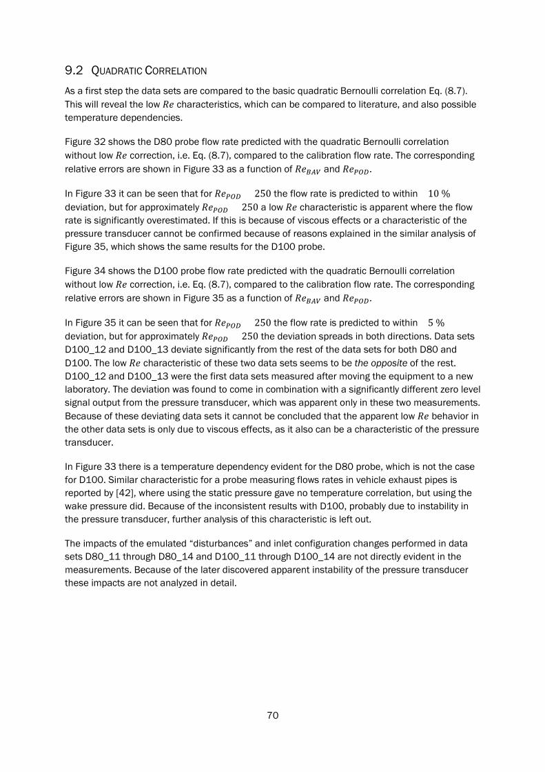
70

9.2 QUADRATIC CORRELATION As a first step the data sets are compared to the basic quadratic Bernoulli correlation Eq. (8.7). This will reveal the low 𝑅𝑅𝑅𝑅 characteristics, which can be compared to literature, and also possible temperature dependencies.

Figure 32 shows the D80 probe flow rate predicted with the quadratic Bernoulli correlation without low 𝑅𝑅𝑅𝑅 correction, i.e. Eq. (8.7), compared to the calibration flow rate. The corresponding relative errors are shown in Figure 33 as a function of 𝑅𝑅𝑅𝑅𝐵𝐵𝐵𝐵𝐵𝐵 and 𝑅𝑅𝑅𝑅𝑃𝑃𝑃𝑃𝑃𝑃.

In Figure 33 it can be seen that for 𝑅𝑅𝑅𝑅𝑃𝑃𝑃𝑃𝑃𝑃 > 250 the flow rate is predicted to within ±10 % deviation, but for approximately 𝑅𝑅𝑅𝑅𝑃𝑃𝑃𝑃𝑃𝑃 < 250 a low 𝑅𝑅𝑅𝑅 characteristic is apparent where the flow rate is significantly overestimated. If this is because of viscous effects or a characteristic of the pressure transducer cannot be confirmed because of reasons explained in the similar analysis of Figure 35, which shows the same results for the D100 probe.

Figure 34 shows the D100 probe flow rate predicted with the quadratic Bernoulli correlation without low 𝑅𝑅𝑅𝑅 correction, i.e. Eq. (8.7), compared to the calibration flow rate. The corresponding relative errors are shown in Figure 35 as a function of 𝑅𝑅𝑅𝑅𝐵𝐵𝐵𝐵𝐵𝐵 and 𝑅𝑅𝑅𝑅𝑃𝑃𝑃𝑃𝑃𝑃.

In Figure 35 it can be seen that for 𝑅𝑅𝑅𝑅𝑃𝑃𝑃𝑃𝑃𝑃 > 250 the flow rate is predicted to within ±5 % deviation, but for approximately 𝑅𝑅𝑅𝑅𝑃𝑃𝑃𝑃𝑃𝑃 < 250 the deviation spreads in both directions. Data sets D100_12 and D100_13 deviate significantly from the rest of the data sets for both D80 and D100. The low 𝑅𝑅𝑅𝑅 characteristic of these two data sets seems to be the opposite of the rest. D100_12 and D100_13 were the first data sets measured after moving the equipment to a new laboratory. The deviation was found to come in combination with a significantly different zero level signal output from the pressure transducer, which was apparent only in these two measurements. Because of these deviating data sets it cannot be concluded that the apparent low 𝑅𝑅𝑅𝑅 behavior in the other data sets is only due to viscous effects, as it also can be a characteristic of the pressure transducer.

In Figure 33 there is a temperature dependency evident for the D80 probe, which is not the case for D100. Similar characteristic for a probe measuring flows rates in vehicle exhaust pipes is reported by [42], where using the static pressure gave no temperature correlation, but using the wake pressure did. Because of the inconsistent results with D100, probably due to instability in the pressure transducer, further analysis of this characteristic is left out.

The impacts of the emulated “disturbances” and inlet configuration changes performed in data sets D80_11 through D80_14 and D100_11 through D100_14 are not directly evident in the measurements. Because of the later discovered apparent instability of the pressure transducer these impacts are not analyzed in detail.

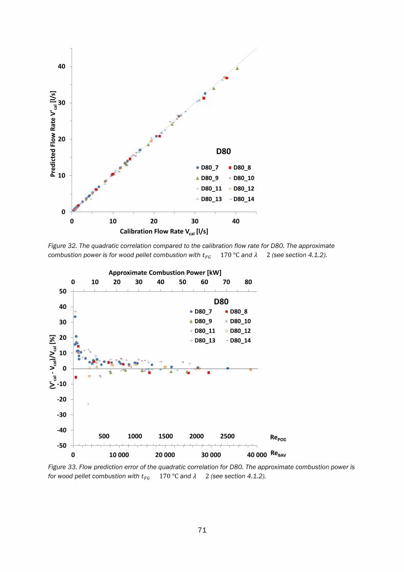
71

Figure 32. The quadratic correlation compared to the calibration flow rate for D80. The approximate combustion power is for wood pellet combustion with 𝑡𝑡𝐹𝐹𝐹𝐹 = 170 °C and 𝜆𝜆 = 2 (see section 4.1.2).

Figure 33. Flow prediction error of the quadratic correlation for D80. The approximate combustion power is for wood pellet combustion with 𝑡𝑡𝐹𝐹𝐹𝐹 = 170 °C and 𝜆𝜆 = 2 (see section 4.1.2).

0

10

20

30

40

0 10 20 30 40

Pred

icte

d Fl

ow R

ate

V'ca

l[l/

s]

Calibration Flow Rate Vcal [l/s]

D80_7 D80_8

D80_9 D80_10

D80_11 D80_12

D80_13 D80_14

D80

0 10 20 30 40 50 60 70 80

-50

-40

-30

-20

-10

0

10

20

30

40

50

0 10 000 20 000 30 000 40 000

Approximate Combustion Power [kW]

(V' ca

l-V c

al)/

V cal

[%]

ReBAV

D80_7 D80_8D80_9 D80_10D80_11 D80_12D80_13 D80_14

D80

500 1000 1500 2000 2500 RePOD

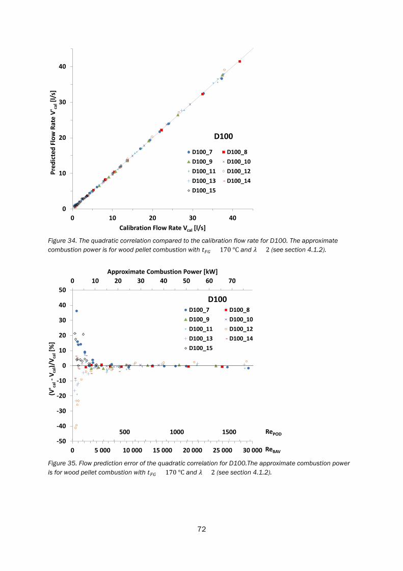
72

Figure 34. The quadratic correlation compared to the calibration flow rate for D100. The approximate combustion power is for wood pellet combustion with 𝑡𝑡𝐹𝐹𝐹𝐹 = 170 °C and 𝜆𝜆 = 2 (see section 4.1.2).

Figure 35. Flow prediction error of the quadratic correlation for D100.The approximate combustion power is for wood pellet combustion with 𝑡𝑡𝐹𝐹𝐹𝐹 = 170 °C and 𝜆𝜆 = 2 (see section 4.1.2).

0

10

20

30

40

0 10 20 30 40

Pred

icte

d Fl

ow R

ate

V'ca

l[l/

s]

Calibration Flow Rate Vcal [l/s]

D100_7 D100_8D100_9 D100_10D100_11 D100_12D100_13 D100_14D100_15

D100

0 10 20 30 40 50 60 70

-50

-40

-30

-20

-10

0

10

20

30

40

50

0 5 000 10 000 15 000 20 000 25 000 30 000

Approximate Combustion Power [kW]

(V' ca

l-V c

al)/

V cal

[%]

ReBAV

D100_7 D100_8D100_9 D100_10D100_11 D100_12D100_13 D100_14D100_15

D100

RePOD500 1000 1500

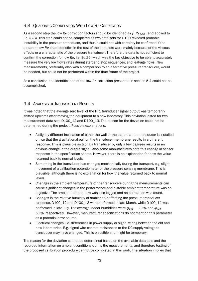
73

9.3 QUADRATIC CORRELATION WITH LOW RE CORRECTION As a second step the low 𝑅𝑅𝑅𝑅 correction factors should be identified as 𝑓𝑓(𝑅𝑅𝑅𝑅𝑃𝑃𝑃𝑃𝑃𝑃) and applied to Eq. (8.8). This step could not be completed as two data sets for D100 revealed probable instability in the pressure transducer, and thus it could not with certainty be confirmed if the apparent low 𝑅𝑅𝑅𝑅 characteristics in the rest of the data sets were mainly because of the viscous effects or a characteristic of the pressure transducer. Therefore the data is not sufficient to confirm the correction for low 𝑅𝑅𝑅𝑅, i.e. Eq.26, which was the key objective to be able to accurately measure the very low flows rates during start and stop sequences, and leakage flows. New measurements, preferably also with a comparison to an alternative pressure transducer, would be needed, but could not be performed within the time frame of the project.

As a conclusion, the identification of the low 𝑅𝑅𝑅𝑅 correction presented in section 5.4 could not be accomplished.

9.4 ANALYSIS OF INCONSISTENT RESULTS It was noted that the average zero level of the PT1 transducer signal output was temporarily shifted upwards after moving the equipment to a new laboratory. This deviation lasted for two measurement data sets D100_12 and D100_13. The reason for the deviation could not be determined during the project. Possible explanations:

• A slightly different inclination of either the wall or the plate that the transducer is installed on, so that the gravitational pull on the transducer membrane results in a different response. This is plausible as tilting a transducer by only a few degrees results in an obvious change in the output signal. Also some manufacturers note this change in sensor response in the specification sheets. However, there is no explanation for how the value returned back to normal levels.

• Something in the transducer has changed mechanically during the transport, e.g. slight movement of a calibration potentiometer or the pressure sensing membrane. This is plausible, although there is no explanation for how the value returned back to normal levels.

• Changes in the ambient temperature of the transducers during the measurements can cause significant changes in the performance and a stable ambient temperature was an objective. The ambient temperature was also logged and no correlation was found.

• Changes in the relative humidity of ambient air affecting the pressure transducer response. D100_12 and D100_13 were performed in late March, while D100_14 was performed in late July. The average indoor humidities were 𝜑𝜑𝑐𝑐𝑅𝑅𝑓𝑓 = 20 % and 𝜑𝜑𝑐𝑐𝑅𝑅𝑓𝑓 =60 %, respectively. However, manufacturer specifications do not mention this parameter as a potential error source.

• Electrical changes, i.e. differences in power supply or signal wiring between the old and new laboratories. E.g. signal wire contact resistances or the DC supply voltage to transducer may have changed. This is plausible and might be temporary.

The reason for the deviation cannot be determined based on the available data sets and the recorded information on ambient conditions during the measurements, and therefore testing of the proposed calibration procedure cannot be completed in this work. The situation implies that

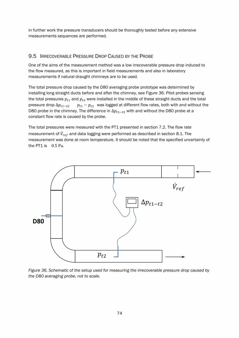
74

in further work the pressure transducers should be thoroughly tested before any extensive measurements sequences are performed.

9.5 IRRECOVERABLE PRESSURE DROP CAUSED BY THE PROBE One of the aims of the measurement method was a low irrecoverable pressure drop induced to the flow measured, as this is important in field measurements and also in laboratory measurements if natural draught chimneys are to be used.

The total pressure drop caused by the D80 averaging probe prototype was determined by installing long straight ducts before and after the chimney, see Figure 36. Pitot probes sensing the total pressures 𝑝𝑝𝑡𝑡1 and 𝑝𝑝𝑡𝑡2 were installed in the middle of these straight ducts and the total pressure drop ∆𝑝𝑝𝑡𝑡1−𝑡𝑡2 = (𝑝𝑝𝑡𝑡1 − 𝑝𝑝𝑡𝑡2) was logged at different flow rates, both with and without the D80 probe in the chimney. The difference in ∆𝑝𝑝𝑡𝑡1−𝑡𝑡2 with and without the D80 probe at a constant flow rate is caused by the probe.

The total pressures were measured with the PT1 presented in section 7.2. The flow rate measurement of �̇�𝑉𝑐𝑐𝑅𝑅𝑓𝑓 and data logging were performed as described in section 8.1. The measurement was done at room temperature. It should be noted that the specified uncertainty of the PT1 is ±0.5 Pa.

Figure 36. Schematic of the setup used for measuring the irrecoverable pressure drop caused by the D80 averaging probe, not to scale.

D80

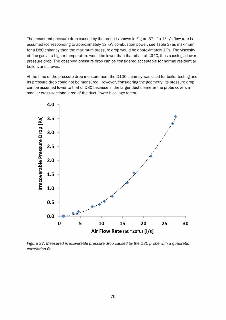
75

The measured pressure drop caused by the probe is shown in Figure 37. If a 13 l/s flow rate is assumed (corresponding to approximately 13 kW combustion power, see Table 3) as maximum for a D80 chimney then the maximum pressure drop would be approximately 1 Pa. The viscosity of flue gas at a higher temperature would be lower than that of air at 20 °C, thus causing a lower pressure drop. The observed pressure drop can be considered acceptable for normal residential boilers and stoves.

At the time of the pressure drop measurement the D100 chimney was used for boiler testing and its pressure drop could not be measured. However, considering the geometry, its pressure drop can be assumed lower to that of D80 because in the larger duct diameter the probe covers a smaller cross-sectional area of the duct (lower blockage factor).

Figure 37. Measured irrecoverable pressure drop caused by the D80 probe with a quadratic correlation fit.

0.0

0.5

1.0

1.5

2.0

2.5

3.0

3.5

4.0

0 5 10 15 20 25 30

Irrec

over

able

Pre

ssur

e D

rop

[Pa]

Air Flow Rate (at ~20°C) [l/s]

76

10 DISCUSSION

Based on the available literature, as described in section 5, the averaging probe shape can be optimized to give both a higher differential pressure output for the same flow rates, and an optimized wake pressure characteristic. Also commercial products with optimized shapes exist, of which one could have been calibrated for low flow rates. The construction used was chosen because of ease of manufacturing at a local workshop, and the possibility to adapt the probe to the desired duct size. Also, earlier research results in literature, regarding e.g. stagnation and wake pressures in low 𝑅𝑅𝑅𝑅 flows, are mostly for round cylinders in cross flows. Using arbitrary cross section shapes (e.g. wing or diamond), either commercial or self-made, would result in difficulties to compare the measurement results to previous research. Optimization of the probe geometry was therefore left out for future work.

More pressure transducers could have been tested to find one with better characteristics (noise, hysteresis, temperature drift etc.). After initial testing, however, a suitable candidate was found, and the problems with long term stability could not be foreseen until the equipment was moved. At this stage most of the data sets were already measured and the measurement sequences could not be repeated within the project.

A thorough uncertainty analysis of the averaging Pitot probe method is not presented. The reason for this is the apparent instability of the pressure transducer. The pressure transducer proved to be a critical component in the method and therefore any conclusions about uncertainty for 𝑅𝑅𝑅𝑅𝑃𝑃𝑃𝑃𝑃𝑃 < 250, approximately, cannot be confirmed until e.g. malfunction of the pressure transducer can be ruled out.

The flow characteristics from combustion (pulsating flow) may be different from a fan induced flow. Also, the measured individual sample points of the data sets are based on steady states, which rarely occur in practice. Further issues are the time constant and the averaging function of the pressure transducer and the possible time lag caused by viscous effects with low 𝑅𝑅𝑅𝑅 flows. Performance of the whole method during transient flows should be determined, and this can be tested e.g. with step changes in the flow rate. The aim of the current work, however, was to test the concept, i.e. whether the low 𝑅𝑅𝑅𝑅 flows present in residential chimneys can be calibrated for.

A comparison of different flow rate measurement methods is not done. There are other methods suitable for continuous measurements, such as orifice plates, venturi tubes, anemometers and particle image velocimetry. The purpose of this study is to evaluate the performance of the standardized Pitot-static method and the averaging Pitot method in low 𝑅𝑅𝑅𝑅 flows, which is needed to be able to do a comparison to other methods.

77

11 CONCLUSIONS

A literature survey and a theoretical study were performed to characterize residential chimney conditions for flue gas flow measurements. The focus is on Pitot-static probes to give sufficient basis for the development and calibration of a velocity pressure averaging probe suitable for continuous measurement of transient flows with the low flow velocities present in residential chimneys.

The pressure averaging probe is a simple remedy to overcome the problems with asymmetric and changing velocity profiles, which the Pitot-static method suffers from, but still keeping low the irrecoverable pressure drop caused by the probe. The experimental results imply that the low flow rate limit of the averaging measurement method depends on the performance of the differential pressure transducer, as the differential pressures produced with normal residential chimney diameters in combination with the chosen probe size are close to the performance limitations of readily available pressure transducers. The pressure transducer chosen in this study had instability, which sets the method performance limitation at and below partial combustion rates of approximately 30 % to 50 %, depending on boiler size and the allowed uncertainty. It should be possible to improve the performance of the method by focusing on finding or building a suitable pressure transducer.

The performance of the averaging method can further be improved by optimizing the geometry of the probe. Another way of improving the uncertainty would be increasing the probe size relative to the conduit diameter to produce a higher differential pressure, with the expense of increasing the irrecoverable pressure drop.

11.1 CHIMNEY FLOW CHARACTERISTICS The flow velocities in residential chimneys from a heating boiler under normal operating conditions are shown to be so low that they in some conditions result in voiding the assumptions of non-viscous fluid, which justify the use of the quadratic Bernoulli equation. A non-linear calibration coefficient as a function of 𝑅𝑅𝑅𝑅 is needed to avoid significant measurement errors due to viscous effects.

The range of 𝑅𝑅𝑅𝑅𝐵𝐵𝐵𝐵𝐵𝐵 < 10 000 during normal boiler operation results in the flow type changing from laminar, across the laminar to turbulent transition region, to fully turbulent flow. This results in significant changes of the velocity profile during continuous measurements of transient flows. In addition, the short duct lengths (after bends and changing duct shapes) used in practice are shown to result in that the measurements are done in the hydrodynamic entrance region, where the flow velocity profiles most likely are neither fully developed nor symmetrical.

Measurements with a realistic chimney setup were done for two internal diameters of 𝐷𝐷𝑖𝑖 =80.5mm and 𝐷𝐷𝑖𝑖 = 104.5mm. The results show that the velocity profiles are both changing significantly (laminar and turbulent characteristics) and are skewed because of bends in the ducts.

78

Single point continuous velocity pressure measurement methods (center point or three quarter radius) are prone to significant errors if the velocity profile is not consistent or predictable.

A measurement method insensitive to velocity profile changes is thus needed, if the flow velocity profile cannot otherwise be determined or predicted with reasonable accuracy for the whole measurement range.

Because of particulate matter and condensing fluids in the flue gas it is beneficial if the probe can be constructed so that it can easily be taken out for cleaning, and equipped with a locking mechanism to always ensure the same alignment in the duct without affecting the calibration.

The literature implies that there may be a significant time lag in the measurements of low flow rates due to viscous effects in the internal impact pressure passages of Pitot probes. The significance in the discussed application has not been studied experimentally in this work, but should be studied in the future.

Care should be taken with the temperature measurement, e.g. with averaging of several sensors, as significant temperature gradients may be present in flue gas ducts.

11.2 EVALUATION OF THE PITOT-STATIC METHOD It is shown that the flow conditions in residential chimneys do not meet the requirements set in ISO 10780 and ISO 3966 for Pitot-static probe measurements, and the methods and their uncertainties are not valid. The main issues are the low flow velocity 𝑣𝑣𝑅𝑅��� < 3 m/s, resulting in ∆𝑝𝑝𝑚𝑚,∞ < 5 Pa and 𝑅𝑅𝑅𝑅𝑃𝑃𝑃𝑃𝑅𝑅 < 600, and significantly changing velocity profiles. The same standards do not provide correction methods for conditions below the given limits for velocity, 𝑅𝑅𝑅𝑅 and differential pressure. In all such cases the measurement method should be calibrated specifically to the application and its whole operating range, and preferably in situ.

In laboratory conditions a carefully in-situ calibrated Pitot-static probe may still perform sufficiently well, with a carefully conditioned flow in combination with the correction method presented in section 2.4.

11.3 EVALUATION OF THE AVERAGING PITOT PROBE The principle of operation of an averaging Pitot probe is presented. The basic characteristics of the stagnation and wake pressures of cylinders in cross flows are studied. Based on these a theory (method) is presented for correcting an averaging pitot probe for low 𝑅𝑅𝑅𝑅 flows.

The literature implies that especially the behavior of the wake, and thus the characteristic of the 𝐶𝐶𝑝𝑝𝑝𝑝, will change with the presence of end plates, which may be a case similar to a closed conduit. The detailed study of this characteristic is left for future work.

79

11.4 DIFFERENTIAL PRESSURE TRANSDUCERS The measured differential pressures from Pitot-static probes in residential chimney flows are so low that the calibration and specified uncertainties of commercially available pressure transducers are not adequate for the purpose. The pressure transducers need to be calibrated specifically for the application, preferably in combination with the probe, and the significance of all different error sources should be investigated carefully.

The characteristics of three industrial standard pressure transducers were tested for suitability for very low differential pressure measurements with the averaging probe prototypes and the calibration rig. Two of the transducers were unsuitable for measuring average flow velocities below 0.4 m/s, which would be required for measuring the flue gas flowrate of a boiler operating at 30 % combustion power, or the low flow rates during start, stop and standby sequences.

The ambient temperature of pressure transducers need to be kept as constant as possible as the temperature drift of the output signal may be a significant error source.

The differential pressure measurement was found to be the weak link in the experimental setup of this work. The pressure transducer PT1 chosen based on initial testing showed long term instability during the measurements sequences, for which the reason could not be determined during the study.

The experience from this study implies that a new calibration needs to be done if the pressure transducer is moved to a new location. E.g. the tilt of the transducer needs to be carefully controlled to ascertain a similar characteristic of the response.

11.5 DEVELOPMENT AND TESTING OF A CALIBRATION METHOD A calibration theory and a method for an averaging Pitot probe are presented. The output signal of a pressure transducer, combined with a temperature measurement, is calibrated by a known flow rate.

A calibration rig with the possibility for variable flow and temperature was designed and constructed.

Two averaging multiport Pitot probe prototypes were designed and constructed. The construction is such that the probes are easy to unmount for cleaning, but still always locked in the same position in the duct.

Several data sets were acquired for both the D80 and D100 prototype probes. Isotherm data sets were measured for deriving the correlations and identifying the parameters. Validation data sets were measured with arbitrary temperatures, emulated varying inlet configurations and disturbances.

The characteristics of the prototypes were compared to a quadratic correlation (simplified Bernoulli’s theorem). Good agreement was found for 𝑅𝑅𝑅𝑅𝑃𝑃𝑃𝑃𝑃𝑃 > 250, which for the studied probes corresponds to 𝑅𝑅𝑅𝑅𝐵𝐵𝐵𝐵𝐵𝐵 > 4000.

80

For D80 the flow rate is predicted to within ±10 % deviation for 𝑅𝑅𝑅𝑅𝑃𝑃𝑃𝑃𝑃𝑃 > 250. For approximately 𝑅𝑅𝑅𝑅𝑃𝑃𝑃𝑃𝑃𝑃 < 250 a low 𝑅𝑅𝑅𝑅 characteristic is apparent where the flow rate is significantly overestimated.

For D100 the flow rate is predicted to within ±5 % deviation for 𝑅𝑅𝑅𝑅𝑃𝑃𝑃𝑃𝑃𝑃 > 250. For approximately 𝑅𝑅𝑅𝑅𝑃𝑃𝑃𝑃𝑃𝑃 < 250 the deviation appears to spread in both directions, instead of consistent overestimation as apparent for D80 and predicted by theory. This apparent characteristic is because two inconsistent data sets and can be tracked back to the moving of the equipment to a new laboratory, which implies instability in the pressure transducer.

A temperature dependency was observed in the D80 probe response, causing the apparently higher spread in the deviation from the quadratic correlation for 𝑅𝑅𝑅𝑅𝑃𝑃𝑃𝑃𝑃𝑃 > 250, compared to the D100. The reason was not further studied because the inconsistent data sets for the D100 probe suggest instability in the pressure transducer that would make conclusions questionable. Similar temperature dependence has been reported for an averaging Pitot probe in a vehicle exhaust pipe [42].

A correction for the low 𝑅𝑅𝑅𝑅𝑃𝑃𝑃𝑃𝑃𝑃 < 250 characteristic could not be made because of the combination of temperature dependency for the D80 probe and two inconsistent data sets for the D100 probe. There are not enough data sets to both explain the apparently different temperature characteristics of the two probes and to validate the low 𝑅𝑅𝑅𝑅 corrections.

The irrecoverable pressure drop caused by the probe was found to be <1 Pa, which is considered acceptable for field measurements and for emulating field conditions in a laboratory by letting the burner operate in realistic natural chimney draught conditions.

81

12 FUTURE WORK

The analysis and results presented leave several questions unanswered and open some new ones, which need to be studied to further develop the averaging Pitot probe measurement method for the low flow velocities present in residential chimneys.

12.1 DETAILED CHARACTERISTICS OF PRESSURE TRANSDUCERS The stability and repeatability of the pressure transducer was found to be a critical factor, and thus a more stable transducer is needed. More transducers need to be tested, studying also the possibility of modification of these transducers for better performance in the presented measurement method. Another possibility is to build a transducer based on OEM pressure sensors, adding amplification and filtering suitable for the purpose.

The impact of ambient factors (such as tilt, temperature and relative humidity) on the performance of the transducers needs to be tested in more detail. Especially the tilt seems to be a critical factor, and tests should be done to find out e.g. whether the transducer should be vertical or horizontal.

12.2 DETAILED CHARACTERISTICS OF THE PRESSURE COEFFICIENTS 𝑪𝑪𝑪𝑪𝑪𝑪 AND 𝑪𝑪𝑪𝑪𝑪𝑪

The characteristics of both 𝐶𝐶𝑝𝑝𝑝𝑝 = 𝑓𝑓(𝑅𝑅𝑅𝑅𝑃𝑃𝑃𝑃𝑃𝑃) and 𝐶𝐶𝑝𝑝𝑝𝑝 = 𝑓𝑓(𝑅𝑅𝑅𝑅𝑃𝑃𝑃𝑃𝑃𝑃) of the probe need to be determined in more detail for the case of nearby walls and non-uniform or changing velocity profiles. This can be done either experimentally or by CFD, or as a combination of both. An important characteristic to determine is the temperature dependency of 𝐶𝐶𝑝𝑝𝑝𝑝, which seems to be a characteristic of a small conduit diameter relative to the probe size, see also section 12.4.

12.3 OPTIMIZATION OF PROBE CROSS SECTION The current probe configuration of round cylinders was chosen because of ease of manufacturing in local workshops, and to be able to compare the results to earlier research.

The probe cross section can be optimized for giving maximum ∆𝑝𝑝𝑚𝑚,𝑝𝑝 while keeping 𝐶𝐶𝑝𝑝𝑝𝑝 = 𝑓𝑓(𝑅𝑅𝑅𝑅) as simple as possible. Extensive work has been done in the area, but most of the studies are for 𝑅𝑅𝑅𝑅𝐵𝐵𝐵𝐵𝐵𝐵 > 12000 and often for even much higher ranges. For these higher 𝑅𝑅𝑅𝑅 regimes the available literature is quite consistent on that sharp edges in the cross section (e.g. a diamond shape) result in the wake being always separated at the same points, thus giving a more predictable 𝐶𝐶𝑝𝑝𝑝𝑝 and better repeatability as some critical changes in the wake are avoided. A study is needed to determine whether this is also true for the laminar region, and to find out which probe cross sections give optimal characteristics for the purpose.

82

12.4 PROBE RESPONSE DEPENDENCY ON THE FLUID FLOW TEMPERATURE

The results for the D80 probe imply a temperature dependency of 𝐶𝐶𝑝𝑝𝑝𝑝, whereas the D100 do not. Also another reported case of temperature dependency for vehicle exhaust pipes was found in recent literature [42]. The temperature dependency with different duct diameters should therefore be studied further.

This is not critical for the calibration of an averaging probe as the detailed characteristics can be treated as a black-box model, but avoiding the calibration with varying temperature would make the calibration procedure much less time consuming and simplifying the calibration rig.

12.5 DETERMINING THE TIME CONSTANT The pressure transducers have a time constant (stabilization time), which needs to be determined so that suitability for measuring short transients can be estimated. The possible time lag caused by viscous effects with low 𝑅𝑅𝑅𝑅 flows may also be significant and needs to be determined experimentally as the available literature on the topic is scarce.

An estimation of the time constant can be done by comparing the transducer output stabilization time to the reference flow rate stabilization. Sudden changes in the reference flow rate can be used as a step test.

12.6 UNCERTAINTY ANALYSIS Due to problems with the equipment, a thorough uncertainty analysis of the method was not done in this study. Extensive tests to prove the long term stability and repeatability of the differential pressure measurement are needed before a calibration and validation can be done.

12.7 IMPACT OF DEPOSITS The impact of clogging was not tested thoroughly. As with the case of the uncertainty analysis, this testing should be done after a suitable differential pressure transducer is found.

83

12.8 DEVELOPING THE AVERAGING METHOD FURTHER FOR FIELD MEASUREMENTS One of the objectives was to develop a method which is applicable also to large scale field measurements of residential boilers in realistic conditions. These field measurements present several challenges:

• Ambient conditions for the pressure transducers may vary significantly. For the chosen transducer instability was an issue already in a controlled environment.

• The probe will most likely be mounted with very short straight settling lengths upstream and downstream. Although the averaging probe is developed with the specific intention to tackle these problems, the performance in extremely varying configurations needs to be validated better.

• Clogging of the probe will probably be more extensive than in laboratory conditions due to boilers operating in non-optimal settings and conditions. The effects of deposits and clogging need to be determined before applied to these conditions.

• Validation of the calibration in field conditions will be difficult and methods need to be developed for this.

84

13 ACKNOWLEDGMENTS This work was mainly performed at Solar Energy Research Center SERC at Dalarna University in Borlänge, Sweden. The people at SERC have always provided an inspiring and supportive ambience.

The research project has been supported by a Marie Curie Early Stage Research Training Fellowship of the European Community’s Sixth Framework Programme under contract number MEST-CT-2005-020498, project ‘Advanced solar heating and cooling for buildings – SOLNET’. The work was performed in collaboration with the project SWX-Energi, which was financed by the European Union, Swedish Energy Agency, Region Dalarna and Region Gävleborg.

I would like to thank my supervisors Chris Bales at Dalarna University and Jan-Olof Dalenbäck at Chalmers University for their support and patience during this lengthy work, which sidetracked off quite a bit from the original plan.

Special thanks go to my colleagues Kaung Myat Win and Tomas Persson at Dalarna University for their collaboration and support in the laboratory, and to Michel Haller at SPF Rapperswil for his collaboration.

Various guest researchers and students stayed at SERC during my time there and I definitely miss our research group (ir)regular ‘crisis meetings’ in the local pub and various dinners and bbq’s with many inspiring multi-cultural discussions.

85

14 NOMENCLATURE

𝐴𝐴𝑖𝑖 [𝑚𝑚2] Duct internal cross section area 𝑏𝑏 [𝑚𝑚] Length, distance between side walls 𝐶𝐶𝑝𝑝 [−] Pressure coefficient 𝐶𝐶𝑝𝑝𝑝𝑝 [−] Stagnation (total, impact, Pitot) pressure coefficient 𝐶𝐶𝑝𝑝𝑝𝑝 [−] Wake (base) pressure coefficient 𝑑𝑑 [𝑚𝑚] Diameter (cylinder) 𝑑𝑑𝑝𝑝𝑝𝑝 [𝑚𝑚] Probe outer diameter 𝑑𝑑𝑝𝑝𝑖𝑖 [𝑚𝑚] Probe impact hole diameter 𝐷𝐷𝑖𝑖 [𝑚𝑚] Duct internal diameter 𝐾𝐾 [−] Pitot-static probe calibration coefficient 𝑙𝑙 [𝑚𝑚] Length 𝑙𝑙𝐻𝐻 [𝑚𝑚] Hydraulic length, characteristic measure �̇�𝑚𝑐𝑐𝑙𝑙𝑙𝑙 [𝑘𝑘𝑘𝑘/𝑠𝑠] Mass flow rate (calibration object) �̇�𝑚𝑐𝑐𝑅𝑅𝑓𝑓 [𝑘𝑘𝑘𝑘/𝑠𝑠] Mass flow rate (calibration reference) 𝑛𝑛 [−] Velocity profile factor 𝑝𝑝 [𝑃𝑃𝑃𝑃] Pressure 𝑝𝑝𝑑𝑑 [𝑃𝑃𝑃𝑃] Dynamic pressure, velocity pressure 𝑝𝑝𝑝𝑝 [𝑃𝑃𝑃𝑃] Pitot pressure, stagnation pressure 𝑝𝑝𝑠𝑠 [𝑃𝑃𝑃𝑃] Local surface node pressure 𝑝𝑝𝑡𝑡 [𝑃𝑃𝑃𝑃] Free stream total pressure 𝑝𝑝𝑑𝑑 + 𝑝𝑝𝑠𝑠 𝑝𝑝∞ [𝑃𝑃𝑃𝑃] Free stream static pressure 𝑃𝑃1 [−] Shape dependent parameter 𝑃𝑃2 [−] Shape dependent parameter 𝑟𝑟𝑝𝑝𝑝𝑝 [𝑚𝑚] Probe outer radius 𝑟𝑟𝑝𝑝𝑖𝑖 [𝑚𝑚] Probe stagnation port radius 𝑅𝑅 [𝑚𝑚] Location on duct radius 𝑅𝑅𝑖𝑖 [𝑚𝑚] Duct internal radius 𝑅𝑅𝑐𝑐 [−] Relative location on duct radius 𝑅𝑅𝑅𝑅 [−] Reynolds number 𝑅𝑅𝑅𝑅𝐵𝐵𝐵𝐵𝐵𝐵 [−] 𝑅𝑅𝑅𝑅 based on 𝑣𝑣𝐵𝐵𝐵𝐵𝐵𝐵 and 𝐷𝐷𝑖𝑖 𝑅𝑅𝑅𝑅𝑃𝑃𝑃𝑃𝑃𝑃 [−] 𝑅𝑅𝑅𝑅 based on probe local 𝑣𝑣 and 𝑑𝑑𝑝𝑝𝑝𝑝 𝑅𝑅𝑅𝑅𝑃𝑃𝑃𝑃𝑅𝑅 [−] 𝑅𝑅𝑅𝑅 based on probe local 𝑣𝑣 and 𝑟𝑟𝑝𝑝𝑝𝑝 𝑅𝑅𝑅𝑅𝑃𝑃𝑃𝑃𝑅𝑅 [−] 𝑅𝑅𝑅𝑅 based on probe local 𝑣𝑣 and 𝑟𝑟𝑝𝑝𝑖𝑖 𝑅𝑅𝑅𝑅𝑐𝑐𝑐𝑐𝑖𝑖𝑡𝑡 [−] Critical 𝑅𝑅𝑅𝑅 (transition between laminar and turbulent flow types) 𝑡𝑡𝑐𝑐𝑙𝑙𝑙𝑙 [º𝐶𝐶] Fluid temperature (calibration object) 𝑇𝑇𝑐𝑐𝑙𝑙𝑙𝑙 [𝐾𝐾] Fluid temperature (calibration object) 𝑡𝑡𝐹𝐹𝐹𝐹 [º𝐶𝐶] Flue gas temperature 𝑡𝑡𝑐𝑐𝑅𝑅𝑓𝑓 [º𝐶𝐶] Fluid temperature (calibration reference) 𝑇𝑇𝑐𝑐𝑅𝑅𝑓𝑓 [𝐾𝐾] Fluid temperature (calibration reference)

86

𝑈𝑈𝐻𝐻 [𝑚𝑚] Characteristic hydrodynamic measure (e.g. radius, diameter or length) 𝑈𝑈𝑐𝑐𝑙𝑙𝑙𝑙,0 [𝑉𝑉] Pressure transducer (calibration object) output voltage at ∆𝑝𝑝𝑐𝑐𝑙𝑙𝑙𝑙 = 0 𝑈𝑈𝑐𝑐𝑙𝑙𝑙𝑙 [𝑉𝑉] “Zeroed” output voltage 𝑈𝑈𝑐𝑐𝑙𝑙𝑙𝑙 = 𝑈𝑈𝑐𝑐𝑙𝑙𝑙𝑙,𝑚𝑚 − 𝑈𝑈𝑐𝑐𝑙𝑙𝑙𝑙,0 (calibration object) 𝑈𝑈𝑐𝑐𝑙𝑙𝑙𝑙,𝑚𝑚 [𝑉𝑉] Pressure transducer (calibration object) output voltage, measured 𝑣𝑣 [𝑚𝑚 𝑠𝑠⁄ ] Fluid velocity 𝑣𝑣0 [𝑚𝑚 𝑠𝑠⁄ ] Fluid velocity at duct center axis 𝑣𝑣𝑐𝑐𝑙𝑙𝑙𝑙 [𝑚𝑚/𝑠𝑠] Fluid velocity (average velocity at calibration object) 𝑣𝑣𝑙𝑙𝑙𝑙𝑚𝑚 [𝑚𝑚 𝑠𝑠⁄ ] Local velocity in laminar flow case 𝑣𝑣𝑡𝑡𝑡𝑡𝑐𝑐𝑡𝑡 [𝑚𝑚 𝑠𝑠⁄ ] Local velocity in turbulent flow case 𝑣𝑣𝑅𝑅 [𝑚𝑚 𝑠𝑠⁄ ] Fluid velocity at 𝑅𝑅 𝑣𝑣𝑅𝑅��� [𝑚𝑚 𝑠𝑠⁄ ] Average fluid velocity over 𝑅𝑅 (average bulk velocity) 𝑣𝑣𝑅𝑅𝑐𝑐 [𝑚𝑚 𝑠𝑠⁄ ] Fluid velocity at 𝑅𝑅𝑐𝑐 �̇�𝑉𝑐𝑐𝑙𝑙𝑙𝑙 [𝑚𝑚3 𝑠𝑠⁄ ] Fluid volume flow rate (calibration object) �̇�𝑉𝑐𝑐𝑙𝑙𝑙𝑙′ [𝑚𝑚3 𝑠𝑠⁄ ] Fluid volume flow rate (calibration object, predicted) �̇�𝑉𝑐𝑐𝑅𝑅𝑓𝑓 [𝑚𝑚3 𝑠𝑠⁄ ] Fluid volume flow rate (calibration reference) 𝑥𝑥𝑓𝑓𝑑𝑑 [𝑚𝑚] Length to achieve fully developed flow velocity profile Greek symbols 𝜈𝜈 [𝑚𝑚2 𝑠𝑠⁄ ] Fluid kinematic viscosity 𝜆𝜆 [−] Combustion excess air ratio 𝜂𝜂 [−] Thermal efficiency 𝜔𝜔 [−] Moisture content of fuel (wet basis) 𝜌𝜌 [𝑘𝑘𝑘𝑘 𝑚𝑚3⁄ ] Fluid density 𝜌𝜌𝑐𝑐𝑙𝑙𝑙𝑙 [𝑘𝑘𝑘𝑘 𝑚𝑚3⁄ ] Fluid density (calibration object) 𝜌𝜌𝑐𝑐𝑅𝑅𝑓𝑓 [𝑘𝑘𝑘𝑘 𝑚𝑚3⁄ ] Fluid density (calibration reference) Δ𝑝𝑝 [𝑃𝑃𝑃𝑃] Differential pressure (velocity pressure) ∆𝑝𝑝𝑚𝑚 [𝑃𝑃𝑃𝑃] Differential pressure (measured) ∆𝑝𝑝𝑚𝑚,𝑝𝑝 [𝑃𝑃𝑃𝑃] Differential pressure (measured) referenced to the wake pressure ∆𝑝𝑝𝑚𝑚,∞ [𝑃𝑃𝑃𝑃] Differential pressure (measured) referenced to the static pressure ∆𝑝𝑝𝑐𝑐𝑙𝑙𝑙𝑙 [𝑃𝑃𝑃𝑃] Differential pressure (calibration object) ∆𝑝𝑝𝑐𝑐𝑅𝑅𝑓𝑓 [𝑃𝑃𝑃𝑃] Differential pressure (calibration reference) Acronyms 𝐷𝐷80 Chimney with 𝐷𝐷𝑖𝑖 = 80𝑚𝑚𝑚𝑚 𝐷𝐷100 Chimney with 𝐷𝐷𝑖𝑖 = 100𝑚𝑚𝑚𝑚

87

15 REFERENCES

[1] M. Olsson, “Residential biomass combustion - emissions of organic compounds to air from wood pellets and other new alternatives,” Chalmers University of Technology, 2006.

[2] C. Boman, “Particulate and Gaseous Emissions from Residential Biomass Combustion,” Umeå University, 2005.

[3] H. Hartmann, P. Rossman, P. Turowski, H. Link, and A. Marks, “Staubemissionen aus Holzfeuerungen - Einflussfaktoren und Bestimmungsmethoden,” 2006.

[4] “EN 303-5:2012: (E) - Heating Boilers - Part 5: Heating boilers for solid fuels, manually and automatically stoked, nominal heat output of up to 500 kW - Terminology, requirements, testing and marking,” Brussels, 2014.

[5] F. Fiedler, “Combined solar and pellet heating systems: Study of energy use and CO-emissions,” Mälardalen University, 2006.

[6] R. Kunde, F. Volz, M. Gaderer, and H. Spliethoff, “Felduntersuchungen an Holzpellet-Zentralheizkesseln,” Das Energie-Fachmagazin BWK, vol. 1, pp. 58–66, 2009.

[7] U. Petterson, H. Persson, and M. Johansson, “FBT-04/24 - Låglastkaraktäristik i små pelletsanläggningar,” Borås, 2004.

[8] M. Y. Haller, J. Paavilainen, L. Konersmann, R. Haberl, A. Dröscher, E. Frank, C. Bales, and W. Streicher, “A unified model for the simulation of oil, gas and biomass space heating boilers for energy estimating purposes. Part II: Parameterization and comparison with measurements,” J. Build. Perform. Simul., vol. 4, no. 1, pp. 19–36, 2011.

[9] M. Y. Haller, J. Paavilainen, L. Konersmann, R. Haberl, A. Dröscher, E. Frank, C. Bales, and W. Streicher, “A unified model for the simulation of oil, gas and biomass space heating boilers for energy estimating purposes. Part I: Model development,” J. Build. Perform. Simul., vol. 4, no. 1, pp. 1–18, 2011.

[10] T. Persson, “Combined solar and pellet heating systems for single-family houses  : -How to achieve decreased electricity usage, increased system efficiency and increased solar gains,” KTH - Royal Institute of Technology, 2006.

[11] S. Thiers, B. Aoun, and B. Peuportier, “Experimental characterization, modeling and simulation of a wood pellet micro-combined heat and power unit used as a heat source for a residential building,” Energy Build., vol. 42, no. 6, pp. 896–903, 2010.

[12] “EN 12952:2003 - Water-tube boilers and auxiliary installations - Part 15: Acceptance tests,” Brussels, 2003.

[13] C. Britton and D. Mesnard, “A Performance Summary of Round- and Diamond-Shaped Averaging Pitot-Type Primaries,” Meas. Control, vol. 15, no. 9, pp. 341–350, 1982.

[14] “ISO 3966:2008(E) - Measurement of fluid flow in closed conduits — Velocity area method using Pitot static tubes,” Geneve, 2008.

[15] “ISO 10780:1994 - Stationary source emissions - Measurement of velocity and volume flowrate of gas streams in ducts,” Geneve, 1994.

88

[16] E. Ower and R. C. Pankhurst, The measurement of air flow, 5th ed. Pergamon Press, 1977.

[17] F. A. MacMillan, “Viscous effects on Pitot tubes at low speeds,” J. R. Aero. Soc., vol. 58, pp. 837–839, 1954.

[18] C. W. Hurd, K. P. Chesky, and A. H. Shapiro, “Influence of viscous effects on impact tubes,” J. Appl. Mech., vol. 248, pp. 253–256, 1953.

[19] S. K. S. Boetcher and E. M. Sparrow, “Limitations of the standard Bernoulli equation method for evaluating Pitot/impact tube data,” Int. J. Heat Mass Transf., vol. 50, no. 3–4, pp. 782–788, 2007.

[20] W. G. S. Lester, “The Flow past a Pitot Tube at Low Reynolds Numbers,” 1960.

[21] R. L. Folsom, “Review of the Pitot Tube,” Trans. ASME, vol. 78, pp. 1447–1460, 1956.

[22] S. H. Chue, “Pressure probes for fluid measurement,” Prog. Aerosp. Sci., vol. 16, no. 2, pp. 147–223, 1975.

[23] D. W. Spitzer, Industrial flow measurement, 2nd ed. Research Triangle Park, NC: Instrument Society of America, 1990.

[24] R. A. Robinson, D. Butterfield, D. Curtis, and T. Thompson, “Problems with Pitots - Issues with flow measurement in stacks,” Int. Environ. Technol., no. June, pp. 1–3, 2004.

[25] G. Nyquist, “ITM-rapport 115, Flödesmätningar med pitotrör Provningsjämförelse 2002,” Stockholm, 2002.

[26] G. Nyquist, “ITM rapport 166, Provningsjämförelse 2007,” Stockholm, 2007.

[27] G. Nyquist, “ITM rapport 80, Flödesmätningar med pitotrör Provningsjämförelse 1999,” Stockholm, 1999.

[28] K. M. Win and T. Persson, “Emissions from residential wood pellet boilers and stove characterized into start-up, steady operation and stop emissions,” Energy Fuels, vol. 28, no. 4, pp. 2496–2505, 2014.

[29] F. P. Incropera and D. B. Dewitt, Fundamentals of heat and mass transfer, 4th ed. New York: Wiley, 1996.

[30] B. S. Massey, Mechanics of Fluids. London: Chapman & Hall, 1989.

[31] H. Schlichting and K. Gersten, Boundary-Layer Theory, 8th ed. Berlin Heidelberg: Springer-Verlag, 2000.

[32] D. W. Spitzer, Flow measurement - Practical guides for measurement and control. Research Triangle Park, NC: Instrument Society of America, 1991.

[33] W. Wagner, Wärmeübertragung, 2nd ed. Würzburg: Vogel, 1988.

[34] J. C. Taylor, “Flow measurement by self-averaging Pitot-tubes.,” MEAS. Control, vol. 20, no. 10 , Dec. 1987-Jan. 1988, pp. 145–147, 1988.

[35] W. Y. Ma, “The Averaging Pressure Tubes Flowmeter for the Measurement of the Rate of Airflow in Ventilating Ducts and for the Balancing of Airflow Circuits in Ventilating Systems,” JIHVE, vol. February, pp. 327–349, 1967.

[36] J. R. Cooke, “The Use of Quartz in the Manufacture of Small Diameter Pitot Tubes,” Bedford, 1955.

89

[37] J. L. Bouhy, “Evolution of the Pitot tube sensor,” J. A, vol. 32, no. 3, pp. 83–86, 1991.

[38] V. Seshadri, B. K. Gandhi, S. N. Singh, and R. K. Pandey, “Analysis of the effect of body shape on annubar factor using CFD,” Measurement, vol. 35, no. 1, pp. 25–32, 2004.

[39] B. Dobrowolski, M. Kabaciński, and J. Pospolita, “A mathematical model of the self-averaging Pitot tube,” Flow Meas. Instrum., vol. 16, no. 4, pp. 251–265, 2005.

[40] M. Kabacinski and J. Pospolita, “Numerical and experimental research on new cross-sections of averaging Pitot tubes,” Flow Meas. Instrum., vol. 19, no. 1, pp. 17–27, 2008.

[41] D. Węcel, T. Chmielniak, and J. Kotowicz, “Experimental and numerical investigations of the averaging Pitot tube and analysis of installation effects on the flow coefficient,” Flow Meas. Instrum., vol. 19, no. 5, pp. 301–306, 2008.

[42] D.-S. Oh and C.-H. Lee, “A comparative study of flow rate characteristics of an averaging Pitot tube type flow meter according to H parameters based on two kinds of differential pressure measured at the flow meter with varying air temperature,” J. Mech. Sci. Technol., vol. 25, no. 8, pp. 1961–1967, 2011.

[43] M. M. Zdravkovich, Flow Around Circular Cylinders Volume 2: Applications. New York: Oxford University Press, 2002.

[44] M. M. Zdravkovich, Flow Around Circular Cylinders Volume 1: Fundamentals. New York: Oxford University Press, 1997.

[45] C. Norberg, “An experimental investigation of the flow around a circular cylinder: influence of aspect ratio,” J. Fluid Mech., vol. 258, pp. 287–316, 1994.