Embed Size (px)
Citation preview
Chapter 5: Continuous Random Variables
McClave: Statistics, 11th ed. Chapter 5: Continuous Random Variables
2
Where We’ve Been Using probability rules to find the probability of discrete events
Examined probability models for discrete random variables
McClave: Statistics, 11th ed. Chapter 5: Continuous Random Variables
3
Where We’re Going Develop the notion of a probability distribution for a continuous random variable
Examine several important continuous random variables and their probability models
Introduce the normal probability distribution
5.1: Continuous Probability Distributions A continuous random variable can assume any numerical value within some interval or intervals.
The graph of the probability distribution is a smooth curve called a probability density function, frequency function or probability distribution.
4McClave: Statistics, 11th ed. Chapter 5: Continuous Random Variables
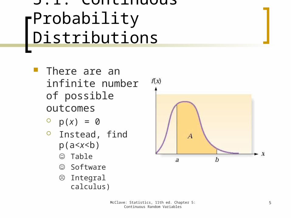
5.1: Continuous Probability Distributions There are an
infinite number of possible outcomes p(x) = 0 Instead, find
p(a<x<b) Table Software Integral
calculus)
5McClave: Statistics, 11th ed. Chapter 5: Continuous Random Variables
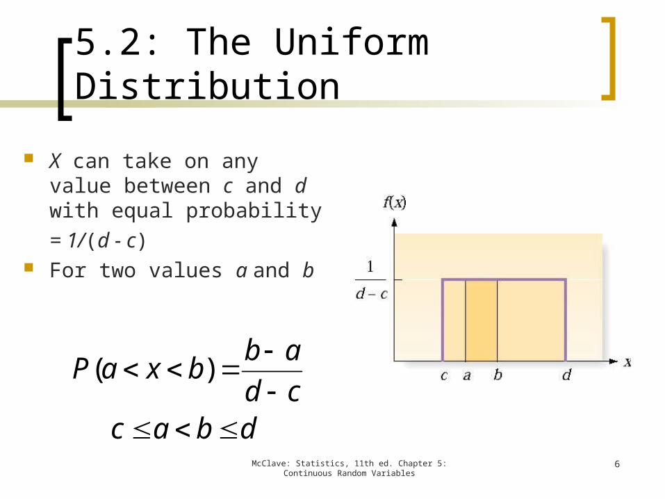
5.2: The Uniform Distribution
X can take on any value between c and d with equal probability= 1/(d - c)
For two values a and b
dbaccdabbxaP
)(
6McClave: Statistics, 11th ed. Chapter 5: Continuous Random Variables
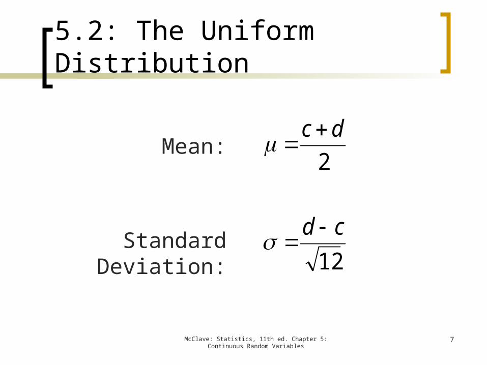
5.2: The Uniform Distribution
Mean:
Standard Deviation: 12
2
cd
dc
7McClave: Statistics, 11th ed. Chapter 5: Continuous Random Variables

5.2: The Uniform Distribution
Suppose a random variable x is distributed uniformly with
c = 5 and d = 25.What is P(10 x 18)?
McClave: Statistics, 11th ed. Chapter 5: Continuous Random Variables
8
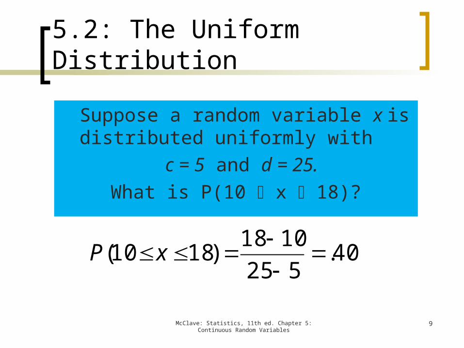
5.2: The Uniform Distribution
Suppose a random variable x is distributed uniformly with
c = 5 and d = 25.What is P(10 x 18)?
McClave: Statistics, 11th ed. Chapter 5: Continuous Random Variables
9
40.5251018)1810(
xP
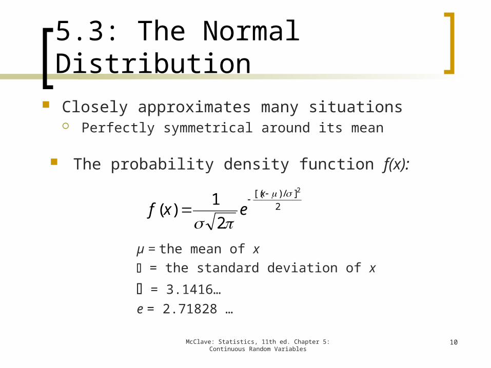
The probability density function f(x):
µ = the mean of x = the standard deviation of x = 3.1416…e = 2.71828 …
5.3: The Normal Distribution
Closely approximates many situations Perfectly symmetrical around its mean
2]/)[( 2
21)(
x
exf
10McClave: Statistics, 11th ed. Chapter 5: Continuous Random Variables
5.3: The Normal Distribution
22
21)(
z
ezf
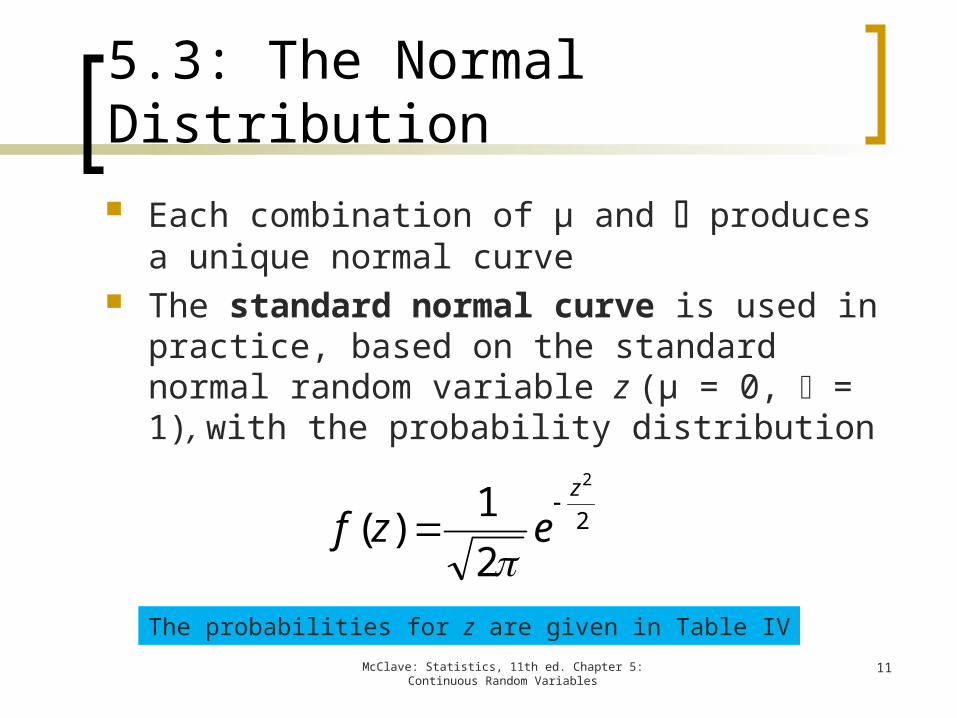
Each combination of µ and produces a unique normal curve
The standard normal curve is used in practice, based on the standard normal random variable z (µ = 0, = 1), with the probability distribution
The probabilities for z are given in Table IV11McClave: Statistics, 11th ed. Chapter 5:
Continuous Random Variables
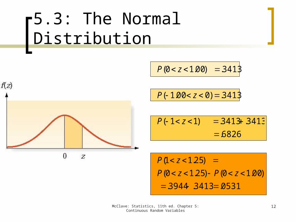
5.3: The Normal Distribution
0531.3413.3944.)00.10()25.10(
)25.11(
6826.3413.3413.)11(
3413.)000.1(
3413.)00.10(
zPzPzP
zP
zP
zP
12McClave: Statistics, 11th ed. Chapter 5: Continuous Random Variables
5.3: The Normal Distribution
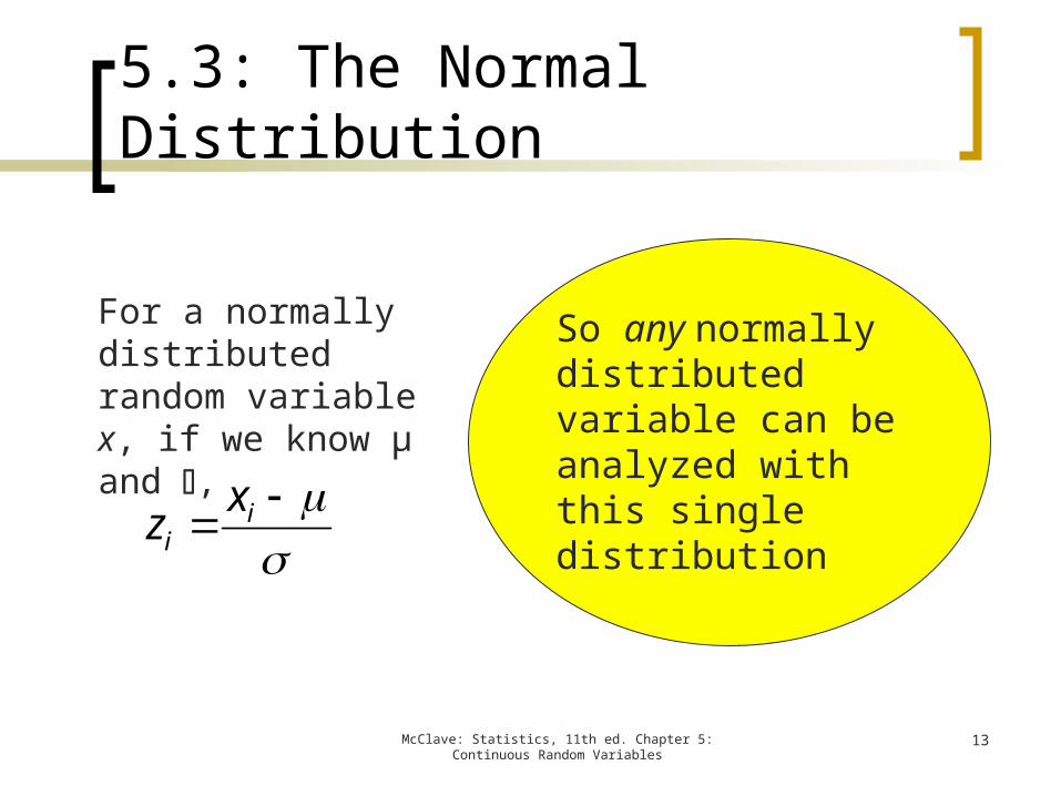
For a normally distributed random variable x, if we know µ and ,
ii
xz
13McClave: Statistics, 11th ed. Chapter 5: Continuous Random Variables
So any normally distributed variable can be analyzed with this single distribution
5.3: The Normal Distribution
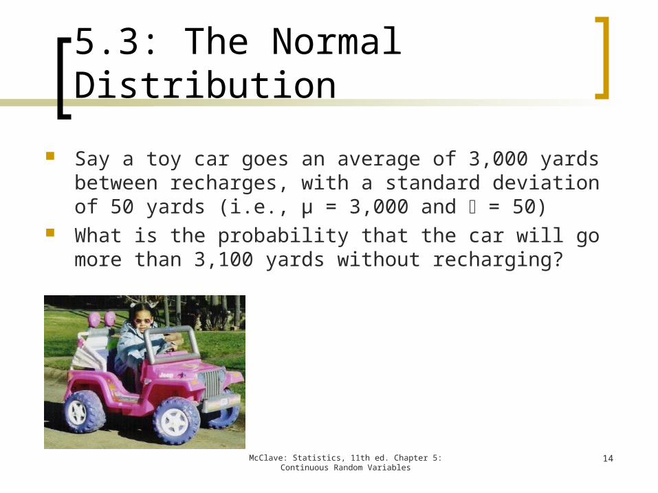
Say a toy car goes an average of 3,000 yards between recharges, with a standard deviation of 50 yards (i.e., µ = 3,000 and = 50)
What is the probability that the car will go more than 3,100 yards without recharging?
14McClave: Statistics, 11th ed. Chapter 5: Continuous Random Variables
5.3: The Normal Distribution
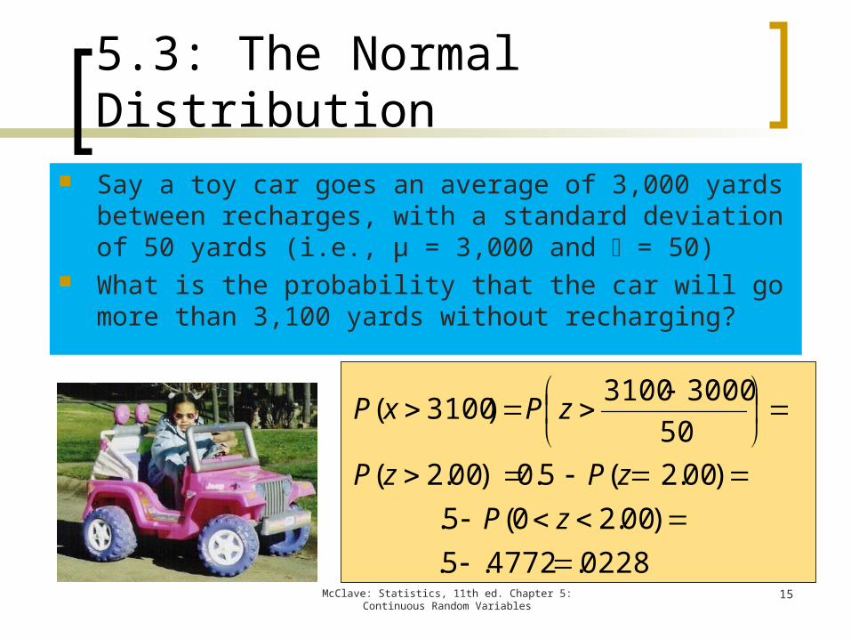
0228.4772.5.)00.20(5.
)00.2(5.0)00.2(5030003100)3100(
zPzPzP
zPxP
Say a toy car goes an average of 3,000 yards between recharges, with a standard deviation of 50 yards (i.e., µ = 3,000 and = 50)
What is the probability that the car will go more than 3,100 yards without recharging?
15McClave: Statistics, 11th ed. Chapter 5: Continuous Random Variables
5.3: The Normal Distribution
To find the probability for a normal random variable … Sketch the normal distribution Indicate x’s mean Convert the x variables into z values Put both sets of values on the sketch, z
below x Use Table IV to find the desired
probabilities
16McClave: Statistics, 11th ed. Chapter 5: Continuous Random Variables
5.4: Descriptive Methods for Assessing Normality
If the data are normal A histogram or stem-and-leaf display will look
like the normal curve The mean ± s, 2s and 3s will approximate the
empirical rule percentages The ratio of the interquartile range to the
standard deviation will be about 1.3 A normal probability plot , a scatterplot with the
ranked data on one axis and the expected z-scores from a standard normal distribution on the other axis, will produce close to a straight line
17McClave: Statistics, 11th ed. Chapter 5: Continuous Random Variables
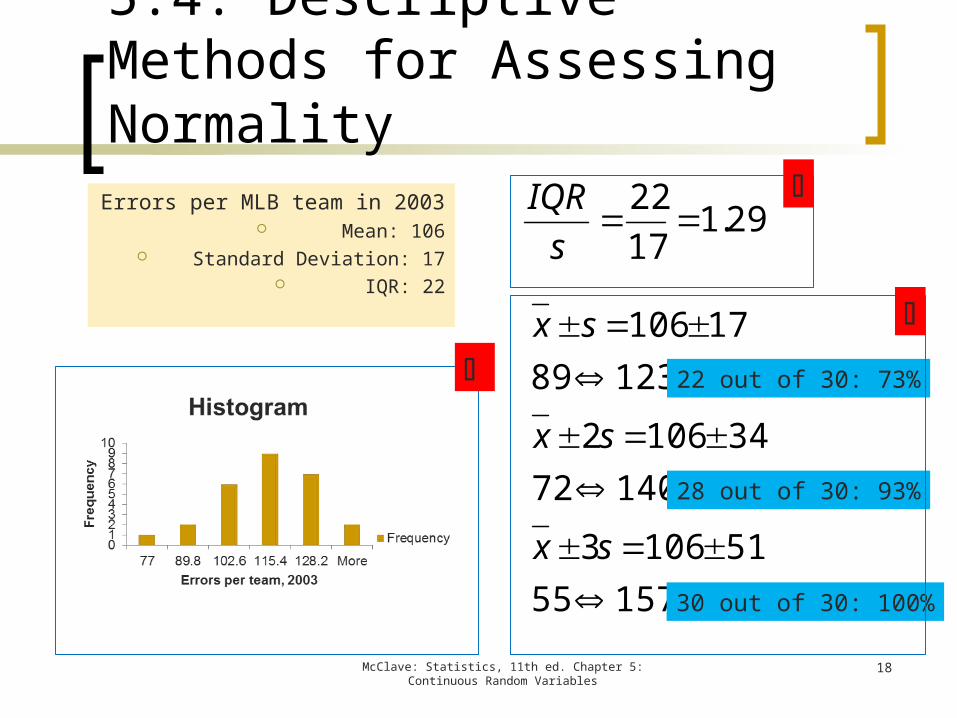
5.4: Descriptive Methods for Assessing NormalityErrors per MLB team in 2003
Mean: 106 Standard Deviation: 17
IQR: 22
29.11722
s
IQR
15755511063
14072341062
1238917106
sx
sx
sx22 out of 30: 73%
28 out of 30: 93%
30 out of 30: 100%
18McClave: Statistics, 11th ed. Chapter 5: Continuous Random Variables
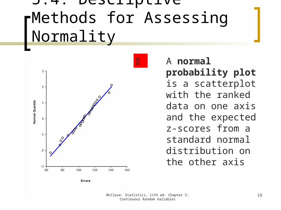
5.4: Descriptive Methods for Assessing Normality
A normal probability plot is a scatterplot with the ranked data on one axis and the expected z-scores from a standard normal distribution on the other axis
19McClave: Statistics, 11th ed. Chapter 5: Continuous Random Variables
5.5: Approximating a Binomial Distribution with the Normal Distribution
Discrete calculations may become very cumbersome
The normal distribution may be used to approximate discrete distributions The larger n is, and the closer p is
to .5, the better the approximation Since we need a range, not a value,
the correction for continuity must be used A number r becomes r+.5
20McClave: Statistics, 11th ed. Chapter 5: Continuous Random Variables
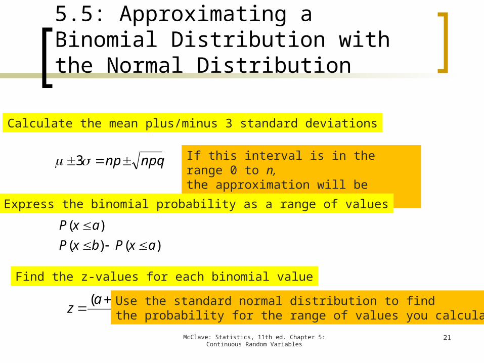
Calculate the mean plus/minus 3 standard deviations
npqnp 3 If this interval is in the range 0 to n, the approximation will be reasonably closeExpress the binomial probability as a range of values
)()()(
axPbxPaxP
Find the z-values for each binomial value
)5.(az Use the standard normal distribution to find
the probability for the range of values you calculated21McClave: Statistics, 11th ed. Chapter 5:
Continuous Random Variables
5.5: Approximating a Binomial Distribution with the Normal Distribution
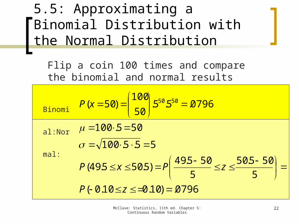
Flip a coin 100 times and compare the binomial and normal results
0796.)10.010.0(5505.50
5505.49)5.505.49(
55.5.100505.100
0796.5.5.50100)50( 5050
zP
zPxP
xP
22McClave: Statistics, 11th ed. Chapter 5: Continuous Random Variables
Binomi
al:Nor
mal:
5.5: Approximating a Binomial Distribution with the Normal Distribution
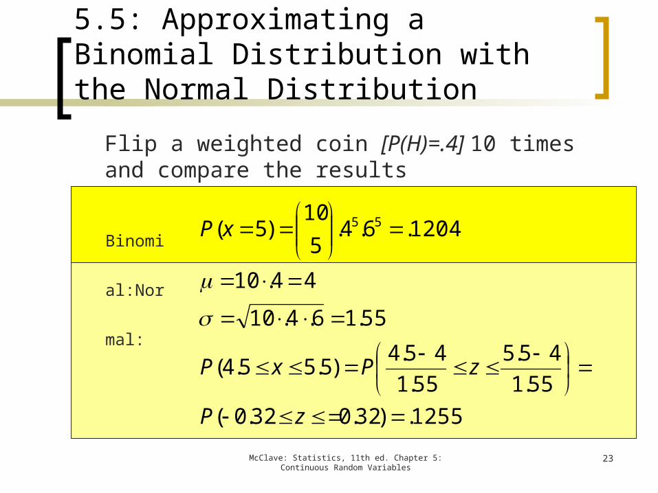
Flip a weighted coin [P(H)=.4] 10 times and compare the results
1255.)32.032.0(55.145.5
55.145.4)5.55.4(
55.16.4.1044.10
1204.6.4.510)5( 55
zP
zPxP
xP
23McClave: Statistics, 11th ed. Chapter 5: Continuous Random Variables
Binomi
al:Nor
mal:
5.5: Approximating a Binomial Distribution with the Normal Distribution
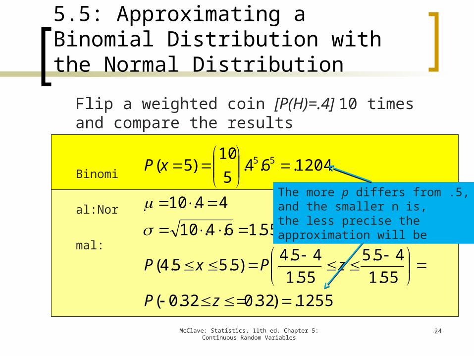
Flip a weighted coin [P(H)=.4] 10 times and compare the results
1255.)32.032.0(55.145.5
55.145.4)5.55.4(
55.16.4.1044.10
1204.6.4.510)5( 55
zP
zPxP
xP
24McClave: Statistics, 11th ed. Chapter 5: Continuous Random Variables
Binomi
al:Nor
mal:
5.5: Approximating a Binomial Distribution with the Normal Distribution
The more p differs from .5, and the smaller n is,the less precise the approximation will be
5.6: The Exponential Distribution
25McClave: Statistics, 11th ed. Chapter 5: Continuous Random Variables
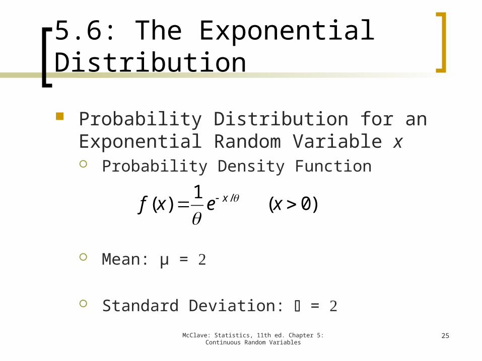
Probability Distribution for an Exponential Random Variable x Probability Density Function
Mean: µ =
Standard Deviation: =
)0(1)( / xexf x
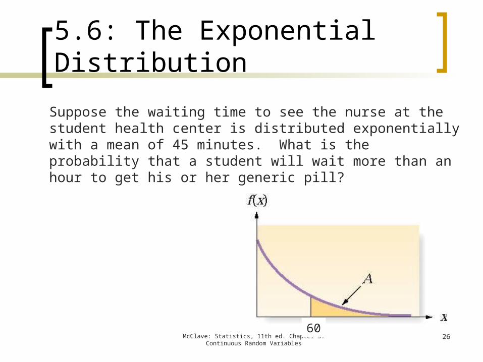
5.6: The Exponential DistributionSuppose the waiting time to see the nurse at the student health center is distributed exponentially with a mean of 45 minutes. What is the probability that a student will wait more than an hour to get his or her generic pill?
McClave: Statistics, 11th ed. Chapter 5: Continuous Random Variables
2660
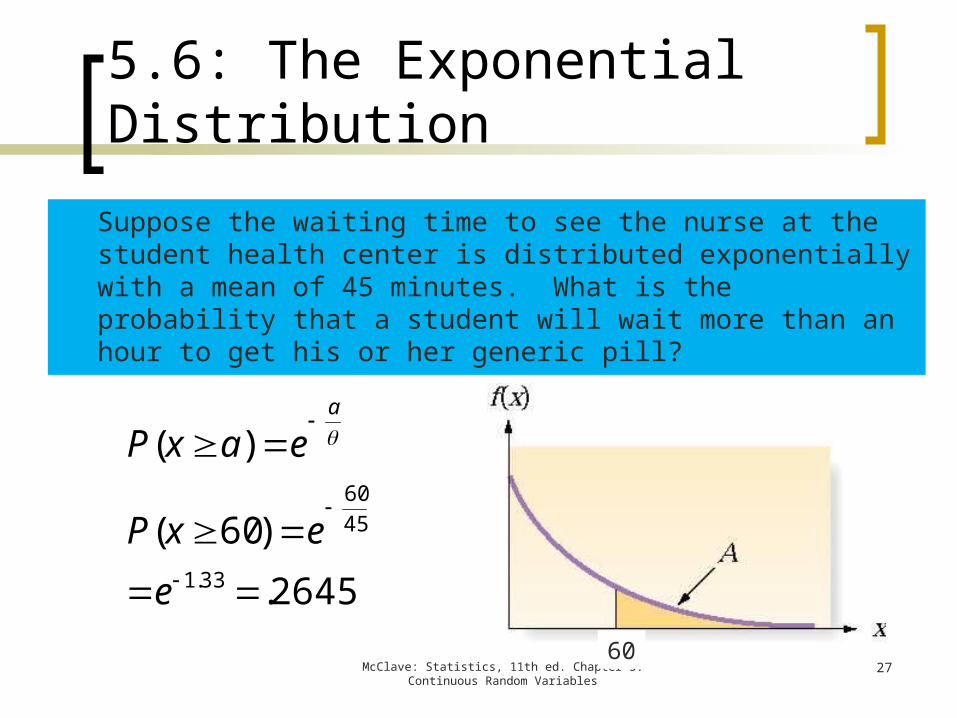
5.6: The Exponential DistributionSuppose the waiting time to see the nurse at the student health center is distributed exponentially with a mean of 45 minutes. What is the probability that a student will wait more than an hour to get his or her generic pill?
McClave: Statistics, 11th ed. Chapter 5: Continuous Random Variables
27
2645.)60(
)(
33.1
4560
eexP
eaxPa
60


