Embed Size (px)
Citation preview

Page No. 89
CHAPTER - 6
ANALYSIS
OF
INVENTORY
MANAGEMENT
This Chapter includes following . . . .1. Introduction of the Chapter2. Inventory Management3. Methods of Inventory Control4. Road map to comparative analysis of
Inventory Management5. Analysis of size of Inventories6. Analysis of Inventories to Current assets7. Analysis of Inventory Circulation8. Output of the chapter

Page No. 90
1. INTRODUCTION OF THE CHAPTERManagement of working capital consists management of all the components ofworking captial. This consists primarily of cash, marketable securities, accountsreceivable and inventory. The balances in these accounts is very crucial because
they are continuously fluctuating. This chapter deals with the issues relating tothe management of inventories.
Inventories occupy the most strategic position in the structure of working capital
of most business enterprises. Also, inventory as a current asset, differs fromother current assets. Because, in management of inventories, only financialmanagers are not involved but all the functional areas of management like
finance, marketing, production and purchasing are jointly involved. The job offinancial manager is to reconcile the conflicting view points of the variousfunctional areas regarding the appropriate level of inventories in order to fulfill
the overall objective of maximising the owner’s wealth.
Since, inventories constitute the largest component of current asset in mostbusiness enterprises, it becomes imperative to manage inventories efficiently
and effectively in order to avoid unnecessary investment. A firm neglecting themanagement of inventories will be jeoparding its long run profitability and mayfail ultimately. It is possible for a company to reduce its level of inventories to a
considerable degree without any adverse effect on production and sales, byusing simple inventory planning and control techniques.
Many of the people understand the word inventory, as a stock of goods, but the
generally accepted meaning of the word ‘goods’ in the accounting language, isthe stock of finished goods only. In a manufacturing organization, however, inaddition to the stock of finished goods, there will be stock of partly finished
goods, raw materials and stores. The collective name of these entire items is‘inventory’. The term invetory refers to the stockpile of production a firm is offeringfor sale and the components that make up the product.1 According to AS - 2,
issued by ICAI, inventories consists of the following.1. Held for sale in ordinary course of business (Finished goods).2. In the process of production of such sale
(Raw material and Work - in - progress)3. In the form of materials or supplies to be consumed in production process or
in rendering the services (Stores, Spares, Consumables etc.) 1
Bolten, SE, Managerial Finance, Houghto Miffin Co., Boston, 1976, P. 426

Page No. 91
Thus various forms of inventories for manufacturing concern are :
1. Raw Material :Raw materials are those basic inputs that are converted into finished productthrough the manufacturing process.
2. Work - in - process :WIP are the semi - manufactured products. They represent products thatneed some more work before they become finished product for sale.
3. Finished goods :Finished goods are those completely manufactured product which are readyfor sale. Stock of raw materials and WIP facilitate production, while stock
of finished goods is required for smooth marketing operations. Thus inventoriesserve as the link between the production and consumption of goods.
4. Supplies (Stores and spares) :Supplies include office and plant cleaning materials like soap, brooms, oil, fuel,light bulbs etc. these materials do not directly enter into the production, butare necessary for the production process. Usually, these supplies are small
part of the total inventories and do not involve significant investment.
So far our study is concerned, inventories comprises nearly 11% of GWC incase of BAL and 28% of GWC in case of HHML. The ideal proportion of
inventories in total current assets can be taken as 15 - 20 % for any manufacturingconcern. Considering this ideal figure, BAL is maintaining very low amount ofinventories while HHML is overstocked. Both the situations are not good for the
health of the organisation.
In this situation it becomes very important to evaluate the inventory managementof both the companies and compare them with each other. To fulfill this purpose,
relevant data of both the companies for the period of ten years from 2000 - 01 to2009 - 10 have been analysed and interpreted.The chapter presents data analysis sheets, certain graphical presentation,
whereever required and the interpretation of the such data analysis.

Page No. 92
2. INVENTORY MANAGEMENT2.1 MEANING
As discussed earlier, there are three types of inventories; Raw materials, Work- in - process and Finished goods. Raw materials are materials and components
that are inputs in making the final product. Work - in - process, also called stock- in - process, refers to goods in the intermediate stages of production. Finishedgoods consist of final products that are ready for sale. While manufacturing
firms generally hold all three types of inventories, distribution firms hold mostlyfinished goods. Inventories represent the second largest asset category formanufacturing companies. Next only to plant and equipment.1
Decisions relating to inventories are taken primarily by executives in productionpurchasing and marketing departments. Usually, raw-material policies areshaped by purchasing and production executives, work - in - process inventory
is influenced by the decisions of production executives, and finished goodsinventory policy is evolved by production and marketing executives. Yet asinventory management has important financial implications, the financial
manager has the responsibility to ensure that inventories are properly monitoredand controlled.1
Management of inventories involves two basic problems.(i) Maintaining a sufficiently large size of inventory for efficient and smooth
production and sales operations.(ii) Maintaining a minimum investment in inventories to minimise the direct -
indirect costs associated with holding inventories to maximise the profitability.Inventories should neither be excessive nor inadequate. If inventories are keptat a high level, higher interest and storage costs would be incurred. On the
other hand, a low level of inventories may result in frequent interruption in theproduction schedule resulting in underutilisation of capacity and lower sales. Itis, therefore, important that investment in inventories should be properly
controlled. The objectives of inventory management, are to a great extent, similarto the objectives of cash management. Inventory management covers a largenumber of problems including fixation of minimum and maximum level of
inventories, determination of size of the inventories to be carried, deciding aboutthe issues, receipts and inspection procedures, proper storage facilities,determining economic oreder quantity, keeping check over obsolescence and
ensuring control over movement of inventories. 1
Chandra Prasanna, “Fundamentals of Financial Management”,(Tata McGraw-Hill Publishing Company Limited, New Delhi,IIIrd ed. 1993) Pp. 21.1

Page No. 93
In short, inventory management should strike a balance between too much
inventory and too little inventory. The efficient management and effective controlof inventories help in achieving better operational results and reducinginvestment in working capital. It has a significant influence on the profitability of
a concern.2.2 IMPORTANCE
To a larger extent, the success or failure of a business depends upon its inventory
management performance. Proper management and control of inventory notonly solve the problems of liquidity but also increases the profitability. Inventoryestablishes link between production and sales. Every business undertaking
needs inventory in adequate quantity for efficient processing and in transithandling. Since inventory itself is an idle investment and involves holding cost,it is always desirable that investment in these assets should be kept at the
minimum possible level. Inventory should be available in proper quantity at alltimes, neither more nor less than what is required. The primary objective ofinventory management is to avoid too much and too little of inventory so that
uninterrupted production and sales with minimum holding costs and bettercustomer services may be possible.
2.3 OBJECTIVESThe aim of inventory management should be to avoid excessive and inadequatelevels of inventories. Efforts should be made to place an order at the right timewith the right sources to acquire the right quality items in right quantity at the
right place. In this sense, the objectives of inventory management can bedescribed as follows.1. Ensuring a continuous supply of materials to production department facilitating
uninterrupted production;2. Maintaining sufficient stock of raw material in the period of short supply;3. Maintaining sufficient stock of finished goods for smooth sales operations;
4. Minimising the carrying costs;5. Keeping investment in inventories at the optimum level.
3. METHODS OF INVENTORY CONTROLThe techinques of inventory management are very useful indetermining theoptimum level of inventory and finding the answers to the problems of economic
order quantity, the re - order point and safety stock. There are some techniquesor methods through which inventory management problems can be handled

Page No. 94
more effficiently and effectively. These methods give broad framework for
managing inventories. Few of them are discussed hereunder. 3.1 PERPETUAL INVENTORY CONTROL SYSTEM3.1.1 Meaning :
The perpetual inventory system is a method of recording stores balances at thetime of each receipt and issue, to facilitate regular checking and to obviateclosing down of work for stock taking. This system is primarily intended as an
aid to material control and in order to ensure accuracy of perpetual inventoryrecords, physical stocks be checked. Thus an essential feature of the perpetualinventory system is the continuous checking of stock.
3.1.2 Operation of perpetual Inventory System :The following is the operation of perpetual inventory system a. As and when materials are received or issued, the quantity is entered in the
bin card and balance is obtained.b. Stores received but not inspected are not mixed up with regular stocks.c. Every day physical stocks are taken for some items and the bin cards/ stores
ledger balances are compared with the physical stock and finally entered inStores Verification Report for adjustment in bin cards and stores ledger.
It may be mentioned that physical stock may be
a. Continuous or perpetual stock taking;b. Periodical stock taking at the end of say each month or each quarter; andc. annual stock taking.
Where records of materials receipt, issues and balances are kept under perpetualinventory system and physical stocks are taken under continuous or perpetualstock taking method one can get the maximum advantages out of the system.
Thus it is advisible that entries relating to receipt, issues and balances are tobe made under perpetual inventory system and a number of items should becounted and checked daily or at frequent intervals and compared with the bin
cards or stores ledger.3.1.3 Advantages :
The maintenance of satisfactory perpetual inventory records has the following
advantages:1. It obviates the need for the physical checking of all stocks at the year end.2. A detailed, reliable check on the stores is obtained.
3. It avoids the dislocation which arises when the stocks are checked at one time.4. Errors, irregularities and loss of stock are readily discovered and thus it helps
in preventing a recurrence in future.

Page No. 95
5. As the work is carried out systematically and without undue haste, the figures
are reliable and planning for production can be done accordingly.6. Actual stock can be compared with the authorized maximum and minimum
levels, thus keeping the stocks within the prescribed limits. The disadvantages
of excess stocks are avoided and capital tied up in stores materials cannotexceed the target.
7. It is possible to prepare monthly or quarterly profit and loss statements and
balance sheet without physical inventory being taken for all the items. :8. It helps in lodging insurance claims for loss on account of fire, theft etc.
3.1.4 Limitations :This system has some limitations too. Unless the Bin Card and Stores Ledgerare kept up to date, effective control cannot be exercised and the work ofcontinuous stocktaking is hampered. It is necessary that the balances shown
by Bin cards and Stores Ledger agree with the actual stock.3.2 FIXATION OF STOCK LEVELS3.2.1 Introduction :
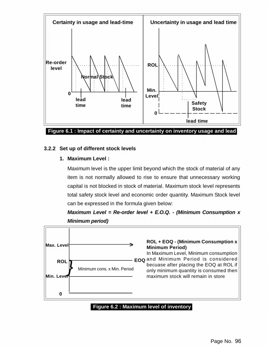
Various levels of stocks are fixed to see that no excess material is carried andsimultaneously there will not be any stockout problems. Fixation of stock levelsdepends upon two important factors,
1. Rate of consumption2. Lead-time (time-gap between placing an order and receiving the materials)
Even these two factors also behave in diferent manner depending upon thesituations. Hence these two factors should be viewed under two differentsituations, say : (a) Under certainty and
(b) Under uncertaintyRate of consumption and lead time can be understood under both the abovesituations with the help of the following figure 6.1
Page No. 96
0
Certainty in usage and lead-time Uncertainty in usage and lead time
Figure 6.1 : Impact of certainty and uncertainty on inventory usage and leadtime
3.2.2 Set up of different stock levels
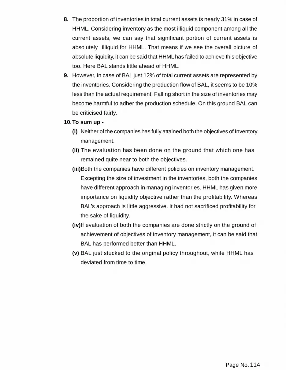
1. Maximum Level :
Maximum level is the upper limit beyond which the stock of material of anyitem is not normally allowed to rise to ensure that unnecessary working
capital is not blocked in stock of material. Maximum stock level representstotal safety stock level and economic order quantity. Maximum Stock levelcan be expressed in the formula given below:
Maximum Level = Re-order level + E.O.Q. - (Minimum Consumption xMinimum period)
Figure 6.2 : Maximum level of inventory
ROL + EOQ - (Minimum Consumption xMinimum Period)In Maximum Level, Minimum consumptionand Minimum Period is consideredbecuase after placing the EOQ at ROL ifonly minimum quantity is consumed thenmaximum stock will remain in store
EOQ} Minimum cons. x Min. Period
>Max. Level
Min. Level
ROL
Re-orderlevel
0leadtime
leadtime
Normal Stock
Min.Level
0
ROL
SafetyStock
lead time

Page No. 97
2. Minimum Level :
Minimum stock level is the lower limit below which the stock of material
of any item should not normally be allowed to fall. This level is also calledsafety stock or emergency stock level. The main object of establishingthis level is to protect against stock out problems, In fixation of minimum
stock level, average rate of consumption and the time required forreplenishment, i.e. lead time are given prime importance.Minimum level = Re-order level - (Normal consumption x Normal period)
Figure 6.3 : Minimum level of inventory
3. Re-Order level :
Re-order level is the level of stock when a new order for the purchase of
material should be placed. The storekeeper will inform the purchasedepartment for the purchase of fresh material when the stock of materialreaches at this level. This level is fixed between the minimum level and
maximum level of stock and the following formula is useful for this purpose.
Re-order level = Maximum Consumption x Maximum Period OR
Re-order level = Minimum stock + (Normal consumption x Normalperiod)
Figure 6.4 : Re - order level of inventory
Max. Level
Min. Level
0
ROLROL - Normal Consumption x Normal
PeriodIn minimum level normal conditions areconsidered i.e. under normal conditions,safety stock should not be used.
Normal cons. x NormalPeriod
Normal cons. x Safety stockperiod
Safety Stock Level
}>
Max. Level
Min. Level
ROLMaximum consumption x Maximum periodIn ROL Max. Cons. and Max. Period areconsidered so as to avoid stock out problems.
0
}>

Page No. 98
4. Danger level :
Danger level is fixed below the minimum level of stock of material and ifstock reaches below this level, urgent action for the fresh purchase ofmaterials should be taken to prevent stockout position.
Danger level= Normal Consumption x Maximum Period forEmergency Purchase
Figure 6.5 : Danger level of inventory5. Average stock :
Average stock = 1/2 (Minimum Level + Maximum Level)
3.3 ECONOMIC ORDERING QUANTITY (EOQ)3.3.1 Meaning
The size of an economic buying quantity or economic purchase lot depends onmany factors such as inventory holding costs and procuring costs. Carryingcosts include interest or cost of capital tied up; warehousing and handling costs;
deterioration; obsolescence; insurance and pilferage. Procuring or ordering costsare the costs of getting a material into the stores and are incurred each time anorder is placed for the purchase of the item. Such ordering costs include cost of
processing purchase orders, receiving and inspection cost and generaladministration overhead comprising salaries, stationery, rent etc. of the purchasedepartment. It may be observed that as the number of units per order is increased
(i.e. less number of purchase orders are issued) ordering costs are reduced butthe holding costs are increased as more units are to be kept in stores. With theinteraction of these two costs the economic ordering quantity will be determined
where the total cost will be minimum. This will happen where holding costs andordering costs are equal (that is at the point of intersection of these lines).
Max. Level
Min. Level
0
ROLNormal Cons. x Normal Period
Normal Stock
DangerLevel
Normal Consumption x Maximum time for emergency
Normal Cons. x Safety stock periodSafety Stock
Normal Cons. x EmergencyPeriod
>

Page No. 99
3.3.2 Assumptions of the modelEOQ model is based on the following assumptions :
(i) The firm knows with certainty the annual usage or demand of the particularitems of inventories.
(ii) The rate at which the firm uses the inventories or makes sales is constant
throughout the year.(ii) The orders for replenishment of inventory are placed exactly when inventories
reach the zero level.
The above assumptions may also be called as limitations of EOQ Model. Onaccount of these reasons, EOQ Model may sometimes give wrong estimateabout economic ordering quantity.
3.3.3 Graphic presentation
Size of Order (Units)
Figure 6.6 : EOQ

Page No. 100
3.3.4 Derrivation of the formula of EOQIf Annual Consumption : A unitsOrdering cost per order : Rs. O
Carrying cost per unit p.a. : Rs. CQuantity purchased at a time : Q unitsThen Total Ordering Cost = (No. of orders × Cost per order)
= A × O ........................... (1)Q
Total Carrying Cost = (Average inventory × Carrying cost per unit p.a.)
= Q × C ........................... (2)2
Total Inventory Cost = Total Ordering Cost + Total Carrying cost
TC = AO + QC [From (1) & (2)] Q 2
d (TC) = - AO + C ........................... (3) dQ Q2 2
For minimum --d (TC) = 0 dQ
- AO + C = 0 [From (3)] Q2 2
AO = C Q2 2
Q2 = 2AO C
Q = 2AO C
EOQ = 2AO C
3.4. ABC ANALYSIS3.4.1 Meaning
Generally, a firm has to maintain different types of materials. All of them are not
equal in value. Some of them are 'high value', some of them are of 'moderatevalue' and some of them are of 'low value'. It is often not possible for the

Page No. 101
management to exercise same degree of control over all items of materials.
Under ABC analysis, items of materials are controlled according to their 'values'or 'financial importance' classifying into 3 categories / groups.A Group - High Value items,
B Group - Moderate Value items andC Group - Low Value itemsThe high value items of materials are controlled more closely then the low value
items of materials.Past experience shows that :High value items of materials represent very low percentage of total number of
items of stock. Moderate value items of materials represent moderate percentageof total number of stock. Low value items of materials represent very highpercentage of total number of items of stock.
ABC analysis can be explained with the help of hypothetical example as follows% of Total % of Total Value
Group Value of Materials Number of Items of Consumption(Units) of Material
A High value / More Costly Items 10% 70% B Moderate value/ Less Costly items 20% 20%
C Low value / Least Costly items 70% 10%Total 100% 100%
The above table makes it clear that :1. 'A' category of items are small in quantity (10% of total units) but they account
for 'high in value' of total consumption of materials (70% of total consumptionof materials).
2. 'B' category of items are 'moderate in quantity' (20% of total units) and theyaccount for 'moderate in value' of total consumption of materials (20% oftotal consumption of materials).
3. 'C' category of items are 'large in quantity' (70% of total units) but they accountfor 'low in value' of total consumption of materials (10% of total consumptionof materials)
Management can exercise a very close control over 'A' category of items ofmaterials since greatest monetary advantage will come by controlling theseitems. Special attention should be given in estimating their requirements,
determining maximum level, minimum level, re-order level and danger levels.Similarly, other techniques of material control should also be applied to 'A'

Page No. 102
category of items. Since, 'A' category of items constitute the bulk of investmentof working capital fund, it would be worthwhile to bring them under close controland apply modern material control techniques. However, occasional or moderate
control over 'B' category of items of materials may be considered satisfactoryand the frequent purchases and issues of these items may be so planned as tokeep them at minimum level. A little more attention should be given towards this
group of items and their purchase should be taken at quarterly intervals.Regarding 'C' category of items of materials, control may be exercised in ageneral manner. The purchase of these items should be on annual basis or
once in six months or so. It is obvious that since 'C' category of items do nothave a high value, the total investment in such items will not be large.
3.4.2 Procedure for marking off A,B,C1. Determine the cost and usage of each material over a given period.2. Multiply unit cost by estimated usage to obtain net value.3. List all items with quantity and value and arrange them in descending value.
4. Accumulate value and add up number of items and calculate percentage ontotal inventory in value and in number.
5. Draw a curve of percentage items and percentage value.
6. Mark off from the curve the rational limits of A,B,C categories3.4.3 Chart showing ABC analysis
ABC ANALYSIS
Figure 6.7 : ABC analysis
0
10
20
30
40
50
60
70
80
10 30 100
10 A0
BC
PER
CEN
TAG
E O
F VA
LUE
OF
CO
NSU
MP
TIO
N
PERCENTAGE OF ITEMS OF THE STOCK Consumption Stock

Page No. 103
3.4.4 Advantages of ABC Analysis1. There is a closer control on costly items in which large amount of capital
has been invested.2. Clerical cost can be reduced by placing the order and stock can be maintained
at optimum level.3. It is possible to keep the minimum level of investment in material.4. Equal attention on all the items can be reduced. It helps to concentrate
on items according to the value of consumption.3.4.5 Limitations
In ABC analysis items are controlled according to their money value and not
according to the importance of the item in the production process. It maysometimes create difficulties. For example, an item of material may not be verycostly and hence it may have been put in category 'C'. However, the item may
be very important to the production process because of its scarcity. Such anitem as a matter of fact requires the at most attention of the management thoughit is not advisable to do so as per the system of ABC analysis. Hence, ABC
analysis should not be followed blindly.3.5. VITAL, ESSENTIAL AND DESIRABLE (V.E.D.) ANALYSIS :
This analysis is used generally for Spare-parts. The requirements and urgency
of spare parts and different from that raw materials. ABC analysis may not beproperly used for spare parts. The demand and urgency for spare parts dependsupon the performance of the plant and machinery. The spare parts are classified
into 3 categories / group :V Group - Vital,E Group - Essential and
D Group - DesirableV - Vital spare parts are must for smooth running of the concern and these
must be stored adequately. The non-availability of these spare parts at
the required time may cause stoppage of production. It may disturb theproduction process and even may stop the production process too. (Forexample : Gear Wire in Scooter)
E - Essential spare parts are necessary for smooth running of the concernand these must be stocked in adequate quantity. There should beadequate arrangement for replenishment of these parts at a short notice.
(For example : Break Wire in Scooter)

Page No. 104
D - Desirable items of spare parts do not cause any immediate loss of
production. If the lead-time of these spare parts is less, then stocking ofthese spare parts should be avoided. (For Example : Head Light inscooter)
The classification of items of spare parts is important from the point of view ofproduction. A wrong classification of any item of spare part may create seriousproblem for production process. The classification of spare part should be left
to the technical staff because they know the need, urgency and utility of thesespares.
3.6 JUST - IN - TIME INVENTORY CONTROL3.6.1 Meaning
The just-in-time inventory control system, originally developed by Taichi Oknoof Japan, simply implies that the firm should maintain a minimal level of inventory
and rely on suppliers to provide parts and components "Just-in-time" to meet itsassembly requirements. This may be contrasted with the traditional inventorymanagement system which calls for maintaining a healthy level of safety stock
to provide a reasonable protection against uncertainties of consumption andsupply. The traditional system may be referred to as a "just-in-case" system.
3.6.2 Elements of ProgrammeThe firm may establish a programme of inventory monitoring and controlconsisting of the following elements :
1. Exercise of vigilance against imbalances of raw materials and work-in-processwhich tends to limit the utility of stocks.
2. Vigorous efforts to expendite completion of unfinished production jobs to
get them into saleable condition.3. Active disposal of goods that are surplus, obsolete or unusable.4. Shortening of the production cycle.
5. Change in design to maximise the use of standard parts and components whichare available off-the shelf.
6. Strict adherence to production schedules.
7. Special pricing to dispose of unusually slow-motive items.8. Evening out of seasonal sales fluctuations to the extent possible.

Page No. 105
4. ROAD MAP TO COMPARATIVE ANALYSIS OF INVENTORY MANAGEMENTInventory management of any firm can be analysed in different ways keeping inview the basic objectives of inventory management discussed earlier.Considering the data available to me, I decided to evaluate the inventory
management of both the companies from the following angles, which, ultimately,becomes the road map to comparative analysis of management of inventory.1. Analysis of size of inventories over the years
2. Analysis of inventories to current assets3. Analysis of circulation of inventories
5. ANALYSIS OF SIZE OF INVENTORIES5.1 TABULAR PRESENTATION OF DATA
Table 6.1: Inventories balance of BAL & HHML (2000- 01 to 2009 - 10) (Rupees in Crore)
Year BAL HHML2000 - 01 253.43 198.54
2001 - 02 179.10 178.362002 - 03 207.98 200.922003 - 04 202.56 188.20
2004 - 05 224.17 204.262005 - 06 272.93 226.55
2006 - 07 309.70 275.582007 - 08 349.61 317.102008 - 09 338.84 326.83
2009 - 10 446.21 436.40Min 179.10 178.36Max 446.21 436.40
Avg 278.45 255.27S.D. 83.02 83.12C.V. 29.82 32.56
Source : Table 4.2 and Table 4.3

Page No. 106
5.2 GRAPHICAL PRESENTATION OF DATA
Figure 6.8 : Comparison of Inventory size of BAL & HHML (2000- 01 to 2009 - 10)5.3 DESCRIPTION OF ANALYSIS AND OBSERVATIONS
From the data sheet and figure given above, the following things are analysedand observed.1. The pattern and trend in the investment in inventories for BAL is smooth and
steadily rising. Lowest balance is seen in 2001 - 02 being Rs. 179.10 Cr. andthe highest being Rs. 446.21 Cr. in 2009 - 10. Average of 10 years isRs. 255.27 Cr. There is little movement considering S.D. Rs. 83.02 Cr. and
C.V. 29.02% over the period of 10 years. These figures suggest that investmentin inventories in BAL has continuous trend of rising upward, variations in thesize of inventories is also very low considering C.V. being just 29.02%
2. The pattern and trend in the investment in inventories for HHML is quite similarto that of BAL. Lowest balance is seen in 2001 - 02 being Rs. 178.36 Cr. andthe highest being Rs. 436.40 Cr. in 2009 - 10. Average of 10 years is Rs.
255.27 Cr. There is little movement considering S.D. Rs. 83.12 Cr. and C.V.32.56% over the period of 10 years.
3. If we compare both the companies, on the basis of average amount invested
in the inventories, it is greater in case of BAL compared to HHML. Also asthe C.V is low in BAL compard to HHML, it can be said that BAL’s investmentin inventories is more consistent than HHML. In short, BAL’s investment in
the inventories is consistently higher than that of in HHML.
0
50
100
150
200
250
300
350
400
450
500
2000 - 01
2001 - 02
2002 - 03
2003 - 04
2004 - 05
2005 - 06
2006 - 07
2007 - 08
2008 - 09
2009 - 10
BAL
HHML

Page No. 107
5.4 HYPOTHESIS TETINGFrom the above data it is also reflected that the highest and the lowest balancein the inventories of both the companies are fall in the same year. Also there
seems similar trend over the years so far size of the inventories is concerned.There seems little difference in the average investment in the inventories andfluctuations are also more or less similar. This situation leads us to conclude
that both the companies are on similar path so far the policy regardig size ofinventories is concerned. These results also compel us to test the equality ofboth the companies in this regard.
5.4.1 Null Hypothesis and Alternative HypothesisH0
1 : Size of inventory of BAL is not greater than that of HHMLH1
1 : Size of inventory of BAL is greater than that of HHML
H02 : There is no significant difference between variance in the level of
inventories between two comapanies BAL and HHMLH1
2 : There is significant difference between variance in the level of inventories
between two comapanies BAL and HHML5.4.2 Distribution applicable and the Type of the test
Since the first test is for comparison of average investment in inventories of
both the companies, and sample size is 10, t test will be applicable. Also it is notopen for both the sides, it is one tailed test.The second test is the test for difference or equality of two population variances,
therefore F distribution will be applicable. Also it is open for both the sides, it istwo tailed test.
5.4.3 Summary of useful data for the relevent testsCompany BAL HHMLSample size n1 = 10 n2 = 10Mean 1 = 278.45 2 = 255.27
S.D. s1 = 83.02 s2 = 83.12Variance s1
2 = 6892.32 s22 = 6908.93
5.4.4 Determination of certain values n1 s1
2 = 10 (83.02)2 = 7658.13 (Denominator factor)n1 - 1 10 - 1
n2 s22 = 10 (83.12)2 = 7676.59 (Numerator factor)
n2 - 1 10 - 1
( )
( )
( )
( )

Page No. 108
5.4.5 Table showing value of test statistic and degree of freedom
Test Statistic Degree of freedom Table Value Decision () (5% significance)
t = 0.562 18 1.735 H01 is accepted
F = 1.002 (9, 9) 3.1789 H02 is accepted
5.4.6 Interpretation of the test result1. Inventory size of both the companies is more or less equal. No company is
investing more or less than other, eventhough it looks so from the sample data collected.2. There is no significant difference in the variations of level of inventories
between two companies under study.3. Since the average investments in inventories are equal in both the companies,
as well as variations in the level of investment in the inventories over the years
is also the same, we cannot properly evaluate and compare both the companiesin regard of performance in the management of inventories, unless someother parameters are checked. To evaluate better performance between both
the companies, the scale of activities is required to be taken into consideration.
6. ANALYSIS OF INVENTORIES TO CURRENT ASSETS6.1 TABULAR PRESENTATION OF DATA Table 6.2: Inventories to current assets of BAL & HHML (2000- 01 to 2009 - 10)
Year BAL HHML2000 - 01 0.1229 0.5236
2001 - 02 0.0900 0.31702002 - 03 0.0965 0.42092003 - 04 0.0987 0.3693
2004 - 05 0.0866 0.36792005 - 06 0.0956 0.02822006 - 07 0.0811 0.3013
2007 - 08 0.2119 0.33662008 - 09 0.1457 0.31982009 - 10 0.1487 0.1510
Min 0.0811 0.0282Max 0.2119 0.5236Avg 0.1178 0.3136
S.D. 0.0409 0.1375C.V. 34.69 43.87
Source : Annual Reports of the companies under study for the different years

Page No. 109
6.2 GRAPHICAL PRESENTATION OF DATA
Figure 6.9: Inventories to current assets ratios of BAL & HHML (2000- 01 to 2009 - 10)
6.3 DESCRIPTION OF ANALYSIS AND OBSERVATIONSFrom the data sheet and figure given above, the following things are analysed
and observed.1. Both the companies have completely different pattern of inventories to current
assets ratio.
2. BAL’s inventories to current assets ratio is more or less uniform over the periodof ten years under the study, minimum being 0.0811 times in the year 2006- 07 while maximum being 0.2119 times in the year 2007 - 08. Thus, in these
two years (2006 - 07 & 2007 - 08) span the ratio has becom the most volatileotherwise it has remained almost same near to 0.1 times upto 2005 - 06. Andthenafter little increment is seen in the range of 0.1 times to 0.2 times, upto
the year 2009 - 103. HHML’s inventories to current assets ratio is very high initially in the year 2000
- 01 being 0.5236 times (maximum of last ten years under the study) and then
decreases continuously upto the year 2005 - 06 (except in 2002 - 03) being0.0282 times (minimum of last ten years under the study). Thenafter it showsa rising trend upto 2007 - 08 and then again it falls down continuously during
2008 - 09 and 2009 - 10. Hence, HHML is facing the problem of unstabilityso far the proportion of inventories in current assets is concerned.
0
0.1
0.2
0.3
0.4
0.5
0.6
2000 - 01
2001 - 02
2002 - 03
2003 - 04
2004 - 05
2005 - 06
2006 - 07
2007 - 08
2008 - 09
2009 - 10
BAL
HHML

Page No. 110
4. Average of inventories to current assets ratio is 0.1178 times for BAL whereas
it is 0.3136 times in case of HHML, which is almost 2.7 times higher thanthat of BAL.These figures suggest that higher proportion of current assetsis in the form of inventories in case of HHML comapred to BAL.
5. S.D. of inventories to current assets ratio is 0.0409 times and C.V. is 34.69%in case of BAL while the respective figures for HHML are 0.1375 times and43.87%. Higher C.V. suggests less uniformity and less consistency.
7. ANALYSIS OF CIRCULATION OF INVENTORIES7.1 INTRODUCTION
Considering the fact that the inventory is the most illiquid component among allthe current assets, HHML’s absolute liquidity is under question, because averageproportion of inventory component is very high in total current assets as we
have seen in previous analysis. At the same time, BAL’s situation is also neededto be evaluated further considering that very low proportion of current assets isrepresented by the inventories, which may become crucial for smooth functioning
of production and sales. For these purposes, we need to have analysis of flowof inventories in the organisation. Here, we need to analyse inventories inreference of activity scale. Such analysis would also be helpful in judgeing the
critical area where both the companies face the problem and which one isperforming better.
7.2 MEANING OF CIRCULATION OF INVENTORIESInventory Turnover Ratio shows the number of times the average inventorybalance of company is turned over during the year. The higher the turn over,
the less inventory balance required for any given level of sales and other thingbeing equal, implies greater efficiency. While a low turnover ratio suggests thata large inventory balance is required for a given volume of sales.
7.3 TABULAR PRESENTATION OF DATATable 6.3 : Inventory Turnover Ratio of BAL & HHML (2000- 01 to 2009 - 10)
Year BAL HHML2000 - 01 14.16 16.002001 - 02 23.03 25.072002 - 03 22.81 25.42
2003 - 04 26.75 35.892004 - 05 29.18 42.14

Page No. 111
2005 - 06 31.33 44.57
2006 - 07 34.25 41.922007 - 08 27.72 38.002008 - 09 26.71 41.44
2009 - 10 27.16 38.45Min 14.16 16.00Max 34.25 44.57
Avg 26.31 34.89S.D. 5.48 9.46C.V. 20.82 27.10
Source : Annual Reports of the companies under study for the different years
7.4 GRAPHICAL PRESENTATION OF DATA
Figure 6.10 : Circulation of inventories of BAL & HHML (2000- 01 to 2009 - 10)
7.5 DESCRIPTION OF ANALYSIS AND OBSERVATIONSFrom the data sheet and figure given above, the following things are analysedand observed.1. Both the companies have different flow of inventory circulation in quantum
but similarity in trend.
0
5
10
15
20
25
30
35
40
45
50
2000 -01
2001 -02
2002 -03
2003 -04
2004 -05
2005 -06
2006 -07
2007 -08
2008 -09
2009 -10
BAL
HHML

Page No. 112
2. BAL’s inventory turnover ratio is more or less uniform over the period of ten
years under the study, minimum being 14.16 times in the year 2000 - 01 whilemaximum being 34.25 times in the year 2006 - 07.
3. HHML’s inventory turnover ratio is highly fluctuating over the period of ten
years under the study, minimum being 16 times in the year 2000 - 01 whilemaximum being 44.57 times in the year 2005 - 06.
4. Average of inventory turnover ratio is 26.31 times for BAL whereas it is 34.89
times in case of HHML. These figures suggest that inventory circulation inBAL is slow compared to HHML. HHML can continue its functioning easilyeven with low inventory balance compared to BAL.
5. But seeing average inventory balance of both the companies, eventhough itseems that HHML is maintaining lower inventory balance compared to BAL,actually there is no significant difference between average investment blocked
in the inventories of both the companies, as suggested by the t test (conductedand presented in para. 5.4 of this chapter). This may be becasuse of the riskfactor that HHML is carrying. S.D. of inventory turnover ratio is 5.48 times
and C.V. is 20.82% in case of BAL while the respective figures for HHML are9.46 times and 27.10%. Higher C.V. suggests less uniformity and lessconsistency, resulting higher risk as well.
8. OUTPUT OF THE CHAPTERThe purpose of this chapter was to analyse the inventory management efficiency
of both the companies, in what manner both the companies are on similar trackand where they are different, in the regards of inventory management policy.Which company manages the issues relating to the inventory better should be
the final output of the chapter. The major output revealed from this chapter canbe summarised in the following manner.1. There are basically the two objectives of inventory management. One being
maintaining sufficient inventory balance, so that the production processshould not be held up. And second being, there should not be excessiveinvestment in the inventories, which can adversely affect the profitability of
the business. In short, the goal of inventory management is to maintainideal size of inventory, not too high and not too low, by achieving propertrade - off between profitability and liquidity.

Page No. 113
2. So far our analysis in this chapter is concerned, we have compared both the
companies on three grounds, namely...(1) Level or size of investment in inventories,(2) Proportion of inventory in total current assets and
(3) Inventory circulation flow in the organisation.3. If both the companies are evaluated on all these three parameters jointly,
the correct picture can be judged.
4. Since average inventory circulation is fast in case of HHML, it is havingprevillege of maintaining lower inventory and functioning smoothly resultinghigher profitability. But because of wide fluctuating circulation it could not
exploit the opportunity and had to maintained more or less the same amountof inventory as in case of BAL (which is being suggested by the result of ttest conducted in paragraph 5.4 discussed above.)
The reasons behind this can be judged as :(a) C.V. of ITO ratio for HHML is 27.10% where as it is just 20.82% for BAL.
Higher C.V. implies heavy fluctuations and more risk resulting less
consistency.(b) Because of inventory circulation was highly fluctuating in HHML, it could
not take chance of maintaining lower inventory over the years.
This results suggest inefficiency in the management of inventory on the partof HHML.
5. In short , it can be concluded that HHML has achieved the objective of liquiditybut sacrificed the objective of profitability. It could not achieve proper trade- off between two objectives.
6. So far the situation of BAL is concerned, average investment in inventory isRs. 278.45 Cr., average inventory turnover ratio is 26.31 times and averageof inventory to current assets ratio is approximately 0.12 times. These figures
jointly suggest that inventory circulation is slow compared to HHML. HenceBAL had to maintain more inventory balance to maintain its liquidity. Butsince it is not highly fluctuating because of lower C.V. in all the three ratios,
BAL could continue even with par investment in inventory as HHML,eventhough the situation was not that easy for it.
7. Here we can conclude that BAL has done well so far management of inventory
is concerned. It could utilise its resources better than HHML. BAL hasachieved the trade - off between liquidity and profitability nicely.
Page No. 114
8. The proportion of inventories in total current assets is nearly 31% in case of
HHML. Considering inventory as the most illiquid component among all thecurrent assets, we can say that significant portion of current assets isabsolutely illiquid for HHML. That means if we see the overall picture of
absolute liquidity, it can be said that HHML has failed to achieve this objectivetoo. Here BAL stands little ahead of HHML.
9. However, in case of BAL just 12% of total current assets are represented by
the inventories. Considering the production flow of BAL, it seems to be 10%less than the actual requirement. Falling short in the size of inventories maybecome harmful to adher the production schedule. On this ground BAL can
be criticised fairly.10.To sum up -
(i) Neither of the companies has fully attained both the objectives of Inventory
management.(ii) The evaluation has been done on the ground that which one has
remained quite near to both the objectives.
(iii)Both the companies have different policies on inventory management.Excepting the size of investment in the inventories, both the companieshave different approach in managing inventories. HHML has given more
importance on liquidity objective rather than the profitability. WhereasBAL’s approach is little aggressive. It had not sacrificed profitability forthe sake of liquidity.
(iv)If evaluation of both the companies are done strictly on the ground ofachievement of objectives of inventory management, it can be said thatBAL has performed better than HHML.
(v) BAL just stucked to the original policy throughout, while HHML hasdeviated from time to time.