Embed Size (px)
Citation preview
Ch02. The Simple Regression Model
Ping Yu
HKU Business SchoolThe University of Hong Kong
Ping Yu (HKU) SLR 1 / 78

Definition of the Simple Regression Model
Definition of the Simple Regression Model
Ping Yu (HKU) SLR 2 / 78
Definition of the Simple Regression Model
Definition of the Simple Regression Model
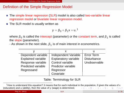
The simple linear regression (SLR) model is also called two-variable linearregression model or bivariate linear regression model.
The SLR model is usually written as
y = β 0+β 1x +u,1
where β 0 is called the intercept (parameter) or the constant term, and β 1 is calledthe slope (parameter).- As shown in the next slide, β 1 is of main interest in econometrics.
y x uDependent variable Independent Variable Error TermExplained variable Explanatory variable DisturbanceResponse variable Control variable UnobservablePredicted variable Predictor variableRegressand Regressor
Covariate
Table: Terminology for SLR
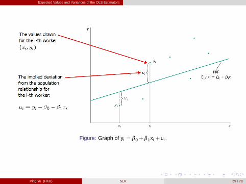
1How to understand this equation? It means that for each individual in the population, if given the values of x(education) and u (ability), then the value of y (wage) is determined.
Ping Yu (HKU) SLR 3 / 78
Definition of the Simple Regression Model
Interpretation of the SLR Model
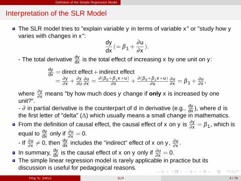
The SLR model tries to "explain variable y in terms of variable x" or "study how yvaries with changes in x":
dydx(= β 1+
∂u∂x).
- The total derivative dydx is the total effect of increasing x by one unit on y :
dydx = direct effect+ indirect effect
= ∂y∂x +
∂y∂u
∂u∂x =
∂ (β 0+β 1x+u)∂x +
∂ (β 0+β 1x+u)∂u
∂u∂x = β 1+
∂u∂x ,
where ∂y∂x means "by how much does y change if only x is increased by one
unit?".- ∂ in partial derivative is the counterpart of d in derivative (e.g., dy
dx ), where d isthe first letter of "delta" (∆) which usually means a small change in mathematics.
From the definition of causal effect, the causal effect of x on y is ∂y∂x = β 1, which is
equal to dydx only if ∂u
∂x = 0.
- If ∂u∂x 6= 0, then dy
dx includes the "indirect" effect of x on y , ∂u∂x .
In summary, dydx is the causal effect of x on y only if ∂u
∂x = 0.The simple linear regression model is rarely applicable in practice but itsdiscussion is useful for pedagogical reasons.
Ping Yu (HKU) SLR 4 / 78
Definition of the Simple Regression Model
Two SLR Examples
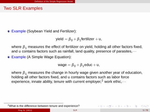
Example (Soybean Yield and Fertilizer):
yield = β 0+β 1fertilizer +u,
where β 1 measures the effect of fertilizer on yield, holding all other factors fixed,and u contains factors such as rainfall, land quality, presence of parasites,� � �Example (A Simple Wage Equation):
wage = β 0+β 1educ+u,
where β 1 measures the change in hourly wage given another year of education,holding all other factors fixed, and u contains factors such as labor forceexperience, innate ability, tenure with current employer,2 work ethic,� � �
2What is the difference between tenure and experience?Ping Yu (HKU) SLR 5 / 78
Definition of the Simple Regression Model
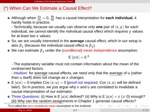
(*) When Can We Estimate a Causal Effect?
Although when ∂u∂x = 0, dy
dx has a causal interpretation for each individual , ithardly holds in practice.- Technically, because we usually can observe only one pair of (x ,y) for eachindividual, we cannot identify the individual causal effect which requires y valuesfor at least two x values.So, we are usually interested in the average causal effect, which in our setup isalso β 1 (because the individual causal effect is β 1).We can estimate β 1 under the (conditional) mean independence assumption:
E [ujx ] = 0.3
- The explanatory variable must not contain information about the mean of theunobserved factors.- Intuition: for average causal effects, we need only that the average of u (ratherthan u itself) does not change as x changes.E [ujx ] = 0 implies Cov (x ,u) = 0 [proof not required, Cov (x ,u) will be definedlater]. So in practice, we just argue why x and u are correlated to invalidate acausal interpretation of our estimator.Three Questions: (i) How is E [ujx ] defined? (ii) Why is E [ujx ] = c ( 6= 0) enough?(iii) Why can the random assignments in Chapter 1 generate causal effects?
3It is called the zero conditional mean assumption in the textbook.Ping Yu (HKU) SLR 6 / 78
Definition of the Simple Regression Model
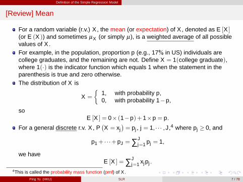
[Review] Mean
For a random variable (r.v.) X , the mean (or expectation) of X , denoted as E [X ](or E (X )) and sometimes µX (or simply µ), is a weighted average of all possiblevalues of X .For example, in the population, proportion p (e.g., 17% in US) individuals arecollege graduates, and the remaining are not. Define X = 1(college graduate),where 1(�) is the indicator function which equals 1 when the statement in theparenthesis is true and zero otherwise.The distribution of X is
X =�
1,0,
with probability p,with probability 1�p,
soE [X ] = 0� (1�p)+1�p = p.
For a general discrete r.v. X , P�X = xj
�= pj , j = 1, � � � ,J,4 where pj � 0, and
p1+ � � �+pJ =∑Jj=1 pj = 1,
we haveE [X ] =∑J
j=1 xjpj .
4This is called the probability mass function (pmf) of X .Ping Yu (HKU) SLR 7 / 78

Definition of the Simple Regression Model
continue
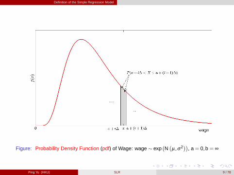
The mean of a continuous r.v. can be defined as an approximation of a discreter.v..
For a continuous r.v. taking values on (a,b), where a can be �∞ and b can be ∞,[figure here]
E [X ] �(b�a)/∆�1
∑i=0
�a+
�i+ 1
2
�∆�
P (a+ i∆ < X � a+(i+1)∆)5
�(b�a)/∆�1
∑i=0
�a+
�i+ 1
2
�∆�
f�
a+�
i+ 12
�∆�
∆ ∆!0�!R ba xf (x)dx .
∑ !R
, a+�
i+ 12
�∆! x , and ∆! dx
For example, if X � N�
µ,σ2�
, the normal distribution with mean µ and variance
σ2, then E [X ] = µ.
Two Useful Properties: (i) "the mean of the sum is the sum of the mean",
Eh∑n
i=1 Xi
i=∑n
i=1 E [Xi ] ; (Xi need not be independent)
(ii) for any constants a and b, E [a+bX ] = a+bE [X ].5 i = 0, a+ i∆ = a, and i = b�a
∆ �1, a+(i+1)∆ = a+ b�a∆ ∆ = b.
Ping Yu (HKU) SLR 8 / 78
Definition of the Simple Regression Model
Figure: Probability Density Function (pdf) of Wage: wage � exp�N�µ,σ2
��, a= 0,b = ∞
Ping Yu (HKU) SLR 9 / 78
Definition of the Simple Regression Model
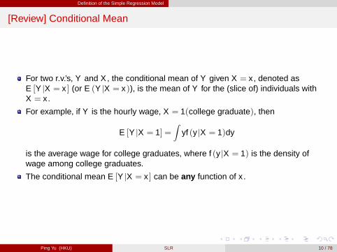
[Review] Conditional Mean
For two r.v.’s, Y and X , the conditional mean of Y given X = x , denoted asE [Y jX = x ] (or E (Y jX = x)), is the mean of Y for the (slice of) individuals withX = x .
For example, if Y is the hourly wage, X = 1(college graduate), then
E [Y jX = 1] =Z
yf (y jX = 1)dy
is the average wage for college graduates, where f (y jX = 1) is the density ofwage among college graduates.
The conditional mean E [Y jX = x ] can be any function of x .
Ping Yu (HKU) SLR 10 / 78
Definition of the Simple Regression Model
continue
One Useful Property: E [g(X )Y jX = x ] = g(x)E [Y jX = x ] for any function g(�),i.e., conditioning on X means X can be treated as a constant.- g(x) is similar to b in the second property of mean.
The two properties of mean can still apply to conditional mean:- (i) "the conditional mean of the sum is the sum of the conditional mean",
Eh∑n
i=1 Yi
���X = xi=∑n
i=1 E [Yi jX = x ] ;
- (ii) for any constants a and b, E [a+bY jX = x ] = a+bE [Y jX = x ].
Ping Yu (HKU) SLR 11 / 78
Definition of the Simple Regression Model
Conditional Mean Independence
Although E [ujx ] can be any function of x , conditional mean independencerestricts it to be the constant zero.
E [ujx ] = 0 means for whatever value x takes, the mean of u given the specific xvalue is zero.
The zero in E [ujx ] = 0 is just a normalization. If E [ujx ] = c 6= 0, then redefineu� = u�c, and β
�0 = β 0+ c. Now,
y = β 0+β 1x +u = (β 0+c)+β 1x +(u�c)� β�0+β 1x +u�,
where E [u�jx ] = E [u�cjx ] = E [ujx ]�c = c�c = 0, and � means "defined as".
So the key here is that E [ujx ] is a constant, not depending on x .- The constant must be E [u] because if the mean of u for each slice of x is c, themean of u for the entire population must be c.
Ping Yu (HKU) SLR 12 / 78
Definition of the Simple Regression Model
E [ujx ] = c and Causal Interpretation: Return to Schooling
Recall the wage equation
wage = β 0+β 1educ+u.
Suppose, for simplicity, educ = 1(college graduate), and u represents the innateability. Then, dwage
deduc should be replaced by E [wagejeduc = 1]�E [wagejeduc = 0].If
E [ujeduc = 1] = c = E [ujeduc = 0] ,
then
E [wagejeduc = 1]�E [wagejeduc = 0] (we can estimate)
= E [β 0+β 1educ+ujeduc = 1]�E [β 0+β 1educ+ujeduc = 0]
= (β 0+β 1)+E [ujeduc = 1]�β 0�E [ujeduc = 0]
= (β 0+β 1)�β 0 = β 1 (the target causal effect).
- Although u is not equal for each individual, averagely, its mean within each groupof education level is equal. This is what "all other relevant factors are balanced" inrandom assignment of x of Chapter 1 means. [If educ is independent of u, thenE [ujeduc] = E [u] = c for whatever value of educ.]The conditional mean independence assumption is unlikely to hold here becauseindividuals with more education will also be more intelligent on average.
Ping Yu (HKU) SLR 13 / 78
Definition of the Simple Regression Model
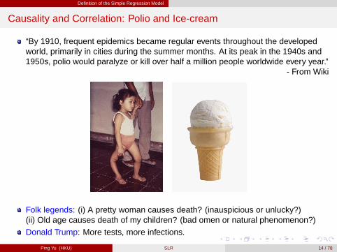
Causality and Correlation: Polio and Ice-cream
“By 1910, frequent epidemics became regular events throughout the developedworld, primarily in cities during the summer months. At its peak in the 1940s and1950s, polio would paralyze or kill over half a million people worldwide every year.”
- From Wiki
Folk legends: (i) A pretty woman causes death? (inauspicious or unlucky?)(ii) Old age causes death of my children? (bad omen or natural phenomenon?)
Donald Trump: More tests, more infections.
Ping Yu (HKU) SLR 14 / 78
Definition of the Simple Regression Model
Population Regression Function (PRF)
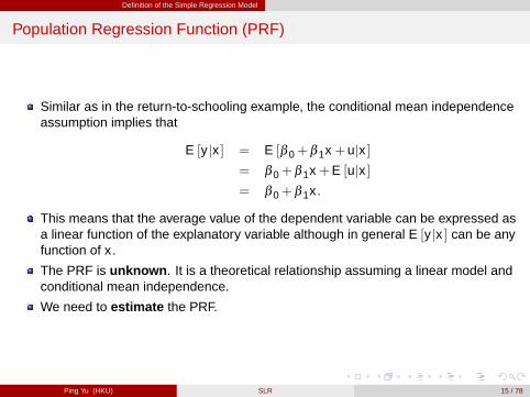
Similar as in the return-to-schooling example, the conditional mean independenceassumption implies that
E [y jx ] = E [β 0+β 1x +ujx ]= β 0+β 1x +E [ujx ]= β 0+β 1x .
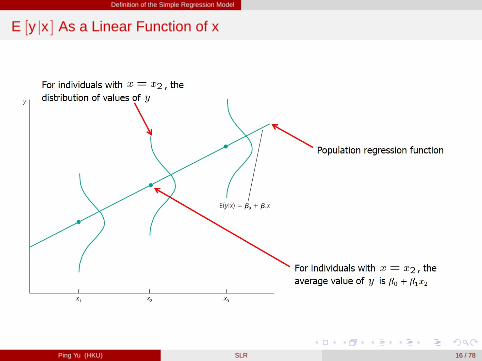
This means that the average value of the dependent variable can be expressed asa linear function of the explanatory variable although in general E [y jx ] can be anyfunction of x .
The PRF is unknown . It is a theoretical relationship assuming a linear model andconditional mean independence.
We need to estimate the PRF.
Ping Yu (HKU) SLR 15 / 78
Definition of the Simple Regression Model
E [y jx ] As a Linear Function of x
Ping Yu (HKU) SLR 16 / 78
Deriving the Ordinary Least Squares Estimates
Deriving the Ordinary Least Squares Estimates
Ping Yu (HKU) SLR 17 / 78
Deriving the Ordinary Least Squares Estimates
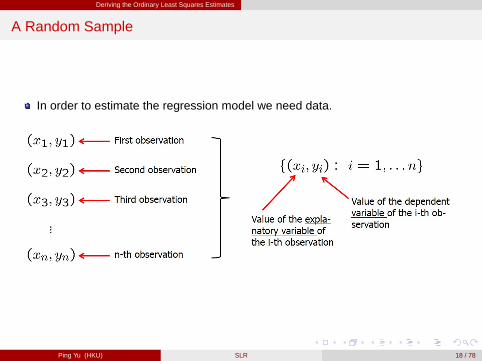
A Random Sample
In order to estimate the regression model we need data.
Ping Yu (HKU) SLR 18 / 78
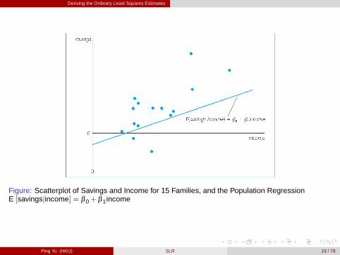
Deriving the Ordinary Least Squares Estimates
Figure: Scatterplot of Savings and Income for 15 Families, and the Population RegressionE [savingsjincome] = β 0+β 1income
Ping Yu (HKU) SLR 19 / 78
Deriving the Ordinary Least Squares Estimates
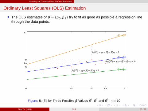
Ordinary Least Squares (OLS) Estimation
The OLS estimates of β = (β 0,β 1) try to fit as good as possible a regression linethrough the data points:
Figure: bui (β ) for Three Possible β Values β1,β 2 and β
3: n = 10
Ping Yu (HKU) SLR 20 / 78
Deriving the Ordinary Least Squares Estimates
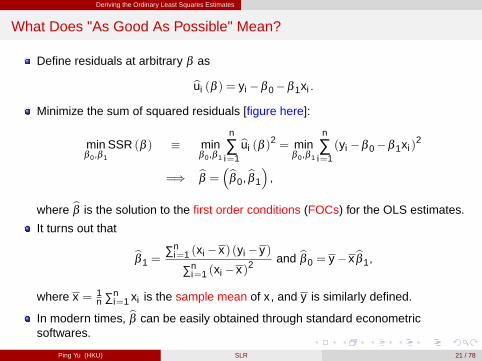
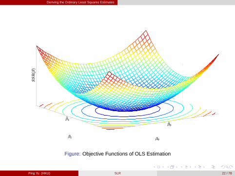
What Does "As Good As Possible" Mean?
Define residuals at arbitrary β as
bui (β ) = yi �β 0�β 1xi .
Minimize the sum of squared residuals [figure here]:
minβ 0,β 1
SSR (β ) � minβ 0,β 1
n
∑i=1
bui (β )2 = min
β 0,β 1
n
∑i=1(yi �β 0�β 1xi )
2
=) bβ = �bβ 0,bβ 1
�,
where bβ is the solution to the first order conditions (FOCs) for the OLS estimates.
It turns out that
bβ 1 =∑n
i=1 (xi �x) (yi �y)
∑ni=1 (xi �x)2
and bβ 0 = y �xbβ 1,
where x = 1n ∑n
i=1 xi is the sample mean of x , and y is similarly defined.
In modern times, bβ can be easily obtained through standard econometricsoftwares.
Ping Yu (HKU) SLR 21 / 78
Deriving the Ordinary Least Squares Estimates
Figure: Objective Functions of OLS Estimation
Ping Yu (HKU) SLR 22 / 78
Deriving the Ordinary Least Squares Estimates
Derivation of OLS Estimates
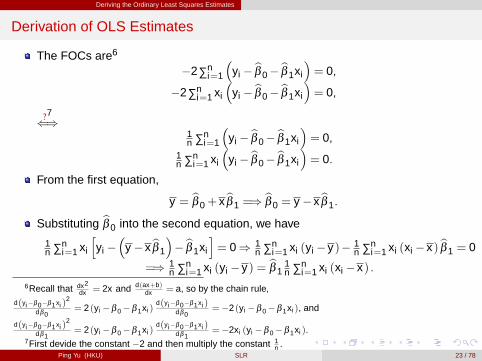
The FOCs are6
�2∑ni=1
�yi � bβ 0� bβ 1xi
�= 0,
�2∑ni=1 xi
�yi � bβ 0� bβ 1xi
�= 0,
?7()
1n ∑n
i=1
�yi � bβ 0� bβ 1xi
�= 0,
1n ∑n
i=1 xi
�yi � bβ 0� bβ 1xi
�= 0.
From the first equation,
y = bβ 0+ xbβ 1 =) bβ 0 = y �xbβ 1.
Substituting bβ 0 into the second equation, we have
1n ∑n
i=1 xi
hyi �
�y �xbβ 1
�� bβ 1xi
i= 0) 1
n ∑ni=1 xi (yi �y)� 1
n ∑ni=1 xi (xi �x) bβ 1 = 0
=) 1n ∑n
i=1 xi (yi �y) = bβ 11n ∑n
i=1 xi (xi �x) .6Recall that dx2
dx = 2x and d(ax+b)dx = a, so by the chain rule,
d(yi�β0�β1xi )2
dβ0= 2 (yi �β 0�β 1xi )
d(yi�β0�β1xi )dβ0
= �2 (yi �β 0�β 1xi ), and
d(yi�β0�β1xi )2
dβ1= 2 (yi �β 0�β 1xi )
d(yi�β0�β1xi )dβ1
= �2xi (yi �β 0�β 1xi ).7First devide the constant �2 and then multiply the constant 1
n .Ping Yu (HKU) SLR 23 / 78
Deriving the Ordinary Least Squares Estimates
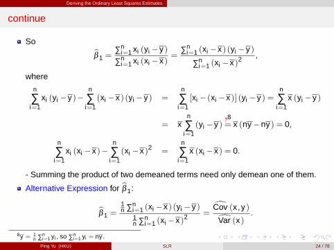
continue
So bβ 1 =∑n
i=1 xi (yi �y)
∑ni=1 xi (xi �x)
=∑n
i=1 (xi �x) (yi �y)
∑ni=1 (xi �x)2
,
where
n
∑i=1
xi (yi �y)�n
∑i=1(xi �x) (yi �y) =
n
∑i=1[xi � (xi �x)] (yi �y) =
n
∑i=1
x (yi �y)
= xn
∑i=1(yi �y)
?8= x (ny �ny) = 0,
n
∑i=1
xi (xi �x)�n
∑i=1(xi �x)2 =
n
∑i=1
x (xi �x) = 0.
- Summing the product of two demeaned terms need only demean one of them.
Alternative Expression for bβ 1:
bβ 1 =1n ∑n
i=1 (xi �x) (yi �y)1n ∑n
i=1 (xi �x)2=dCov (x ,y)dVar (x)
.
8y = 1n ∑n
i=1 yi , so ∑ni=1 yi = ny .
Ping Yu (HKU) SLR 24 / 78
Deriving the Ordinary Least Squares Estimates
[Review] Covariance and Variance
The population covariance between two r.v.’s X and Y , sometimes denoted asσXY , is defined as
Cov (X ,Y ) = E [(X �µX ) (Y �µY )] .
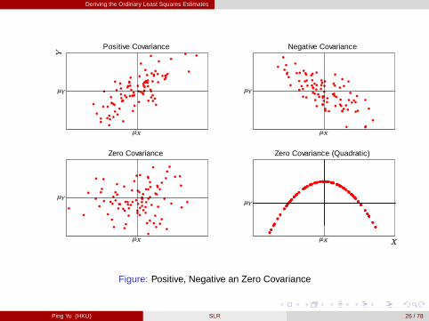
Intuition: [figure here]- If X > µX and Y > µY , then (X �µX ) (Y �µY )> 0, which is also true whenX < µX and Y < µY . While if X > µX and Y < µY , or vice versa, then(X �µX ) (Y �µY )< 0.- If σXY > 0, then, on average, when X is above/below its mean, Y is alsoabove/below its mean. If σXY < 0, then, on average, when X is above/below itsmean, Y is below/above its mean.
A positive covariance indicates that two r.v.’s move in the same direction, while anegative covariance indicates they move in opposite directions.
Ping Yu (HKU) SLR 25 / 78
Deriving the Ordinary Least Squares Estimates
Positive Covariance Negative Covariance
Zero Covariance Zero Covariance (Quadratic)
Figure: Positive, Negative an Zero Covariance
Ping Yu (HKU) SLR 26 / 78
Deriving the Ordinary Least Squares Estimates
continue
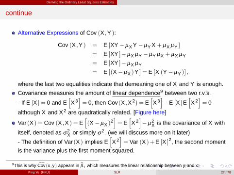
Alternative Expressions of Cov (X ,Y ):
Cov (X ,Y ) = E [XY �µX Y �µY X + µX µY ]
= E [XY ]�µX µY �µY µX + µX µY
= E [XY ]�µX µY
= E [(X �µX )Y ] = E [X (Y �µY )] ,
where the last two equalities indicate that demeaning one of X and Y is enough.
Covariance measures the amount of linear dependence9 between two r.v.’s.
- If E [X ] = 0 and EhX3i= 0, then Cov(X ,X2) = E
hX3i�E [X ]E
hX2i= 0
although X and X2 are quadratically related. [Figure here]
Var (X ) = Cov (X ,X ) = Eh(X �µX )
2i= E
hX2i�µ2
X is the covariance of X with
itself, denoted as σ2X or simply σ2. (we will discuss more on it later)
- The definition of Var (X ) implies EhX2i= Var (X )+E [X ]2, the second moment
is the variance plus the first moment squared.
9This is why dCov(x ,y) appears in bβ 1 which measures the linear relationship between y and x .Ping Yu (HKU) SLR 27 / 78
Deriving the Ordinary Least Squares Estimates
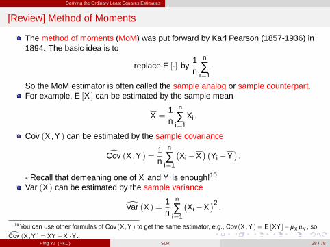
[Review] Method of Moments
The method of moments (MoM) was put forward by Karl Pearson (1857-1936) in1894. The basic idea is to
replace E [�] by1n
n
∑i=1�
So the MoM estimator is often called the sample analog or sample counterpart.For example, E [X ] can be estimated by the sample mean
X =1n
n
∑i=1
Xi .
Cov (X ,Y ) can be estimated by the sample covariance
dCov (X ,Y ) =1n
n
∑i=1
�Xi �X
��Yi �Y
�.
- Recall that demeaning one of X and Y is enough!10
Var (X ) can be estimated by the sample variance
dVar (X ) =1n
n
∑i=1
�Xi �X
�2.
10You can use other formulas of Cov(X ,Y ) to get the same estimator, e.g., Cov(X ,Y ) = E [XY ]�µX µY , sodCov (X ,Y ) = XY �X �Y .Ping Yu (HKU) SLR 28 / 78
Deriving the Ordinary Least Squares Estimates
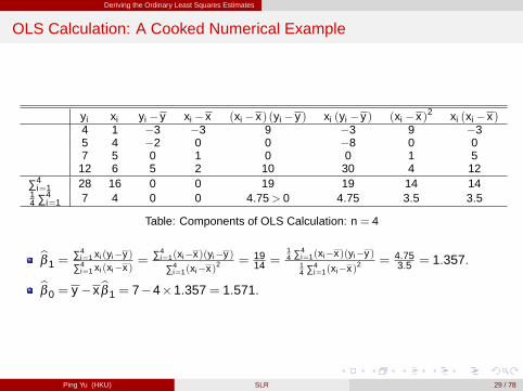
OLS Calculation: A Cooked Numerical Example
yi xi yi �y xi �x (xi �x) (yi �y) xi (yi �y) (xi �x)2 xi (xi �x)4 1 �3 �3 9 �3 9 �35 4 �2 0 0 �8 0 07 5 0 1 0 0 1 5
12 6 5 2 10 30 4 12∑4
i=1 28 16 0 0 19 19 14 1414 ∑4
i=1 7 4 0 0 4.75> 0 4.75 3.5 3.5
Table: Components of OLS Calculation: n = 4
bβ 1 =∑4
i=1 xi (yi�y)∑4
i=1 xi (xi�x)= ∑4
i=1(xi�x)(yi�y)
∑4i=1(xi�x)2
= 1914 =
14 ∑4
i=1(xi�x)(yi�y)14 ∑4
i=1(xi�x)2= 4.75
3.5 = 1.357.
bβ 0 = y �xbβ 1 = 7�4�1.357= 1.571.
Ping Yu (HKU) SLR 29 / 78
Deriving the Ordinary Least Squares Estimates
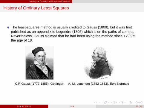
History of Ordinary Least Squares
The least-squares method is usually credited to Gauss (1809), but it was firstpublished as an appendix to Legendre (1805) which is on the paths of comets.Nevertheless, Gauss claimed that he had been using the method since 1795 atthe age of 18.
C.F. Gauss (1777-1855), Göttingen A.-M. Legendre (1752-1833), Éole Normale
Ping Yu (HKU) SLR 30 / 78
Deriving the Ordinary Least Squares Estimates
CEO Salary and Return on Equity
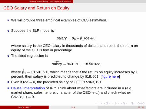
We will provide three empirical examples of OLS estimation.
Suppose the SLR model is
salary = β 0+β 1roe+u,
where salary is the CEO salary in thousands of dollars, and roe is the return onequity of the CEO’s firm in percentage.
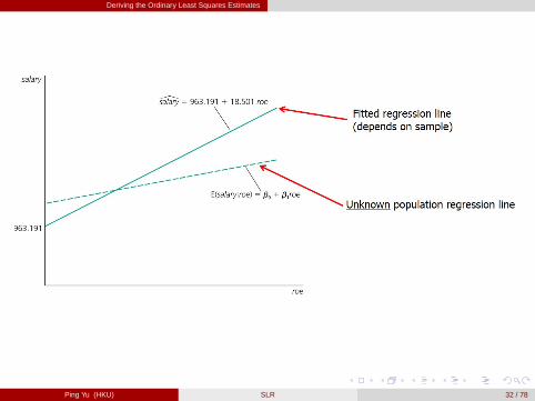
The fitted regression is
\salary = 963.191+18.501roe,
where bβ 1 = 18.501> 0, which means that if the return on equity increases by 1percent, then salary is predicted to change by $18,501. [figure here]
Even if roe = 0, the predicted salary of CEO is $963,191.
Causal Interpretation of bβ 1? Think about what factors are included in u (e.g.,market share, sales, tenure, character of the CEO, etc.) and check whetherCov (x ,u) = 0.
Ping Yu (HKU) SLR 31 / 78
Deriving the Ordinary Least Squares Estimates
Ping Yu (HKU) SLR 32 / 78
Deriving the Ordinary Least Squares Estimates
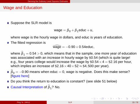
Wage and Education
Suppose the SLR model is
wage = β 0+β 1educ+u,
where wage is the hourly wage in dollars, and educ is years of education.
The fitted regression is\wage = �0.90+0.54educ,
where bβ 1 = 0.54> 0, which means that in the sample, one more year of educationwas associated with an increase in hourly wage by $0.54 (which is quite large!e.g., four years college would increase the wage by $0.54�4= $2.16 per hour,which implies an increase of $2.16�40�52� $4,500 per year).bβ 0 = �0.90 means when educ = 0, wage is negative. Does this make sense?[figure here]
Do you think the return to education is constant? (see slide 51 below)
Causal Interpretation of bβ 1? No.
Ping Yu (HKU) SLR 33 / 78
Deriving the Ordinary Least Squares Estimates
0 2 4 6 8 10 12 14 16 18
00.9
5
10
15
20
25
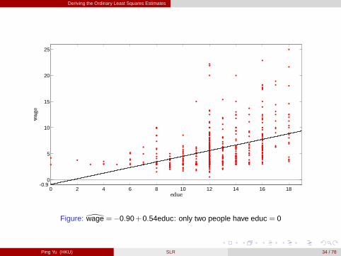
Figure: \wage = �0.90+0.54educ: only two people have educ = 0
Ping Yu (HKU) SLR 34 / 78
Deriving the Ordinary Least Squares Estimates
Voting Outcomes and Campaign Expenditures (Two Parties)
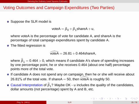
Suppose the SLR model is
voteA= β 0+β 1shareA+u,
where voteA is the percentage of vote for candidate A, and shareA is thepercentage of total campaign expenditures spent by candidate A.
The fitted regression is
\voteA= 26.81+0.464shareA,
where bβ 1 = 0.464> 0, which means if candidate A’s share of spending increasesby one percentage point, he or she receives 0.464 (about one half) percentagepoints more of the total vote.
If candidate A does not spend any on campaign, then he or she will receive about26.81% of the total vote. If shareA= 50, then \voteA is roughly 50.
Causal Interpretation of bβ 1? Maybe OK - u includes the quality of the candidates,dollar amounts (not percentage) spent by A and B, etc.
Ping Yu (HKU) SLR 35 / 78
Properties of OLS on Any Sample of Data
Properties of OLS on Any Sample of Data
Ping Yu (HKU) SLR 36 / 78
Properties of OLS on Any Sample of Data
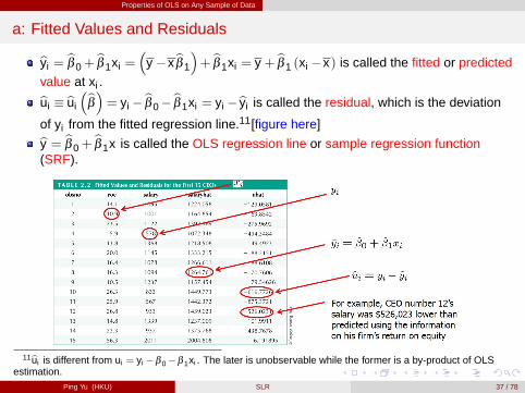
a: Fitted Values and Residuals
byi =bβ 0+
bβ 1xi =�
y �xbβ 1
�+ bβ 1xi = y + bβ 1 (xi �x) is called the fitted or predicted
value at xi .bui � bui
�bβ�= yi � bβ 0� bβ 1xi = yi �byi is called the residual, which is the deviation
of yi from the fitted regression line.11[figure here]by = bβ 0+bβ 1x is called the OLS regression line or sample regression function
(SRF).
11bui is different from ui = yi �β 0�β 1xi . The later is unobservable while the former is a by-product of OLSestimation.
Ping Yu (HKU) SLR 37 / 78
Properties of OLS on Any Sample of Data
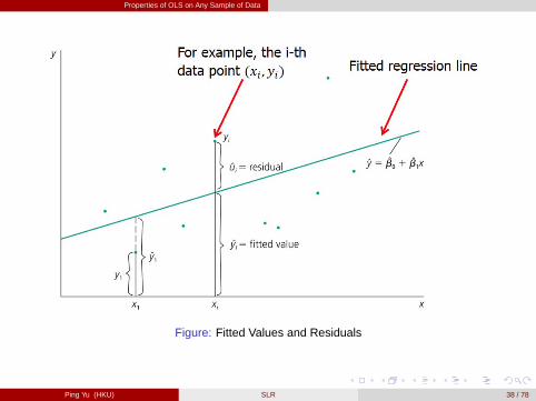
Figure: Fitted Values and Residuals
Ping Yu (HKU) SLR 38 / 78
Properties of OLS on Any Sample of Data
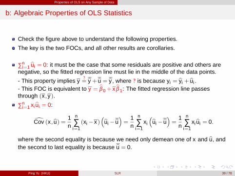
b: Algebraic Properties of OLS Statistics
Check the figure above to understand the following properties.
The key is the two FOCs, and all other results are corollaries.
∑ni=1 bui = 0: it must be the case that some residuals are positive and others are
negative, so the fitted regression line must lie in the middle of the data points.
- This property implies y?= by + bu = by , where ? is because yi = byi + bui .
- This FOC is equivalent to y = bβ 0+ xbβ 1: The fitted regression line passesthrough (x ,y).
∑ni=1 xibui = 0:
dCov (x ,bu) = 1n
n
∑i=1(xi �x)
�bui �bu�= 1n
n
∑i=1
xi
�bui �bu�= 1n
n
∑i=1
xibui = 0.
where the second equality is because we need only demean one of x and bu, andthe second to last equality is because bu = 0.
Ping Yu (HKU) SLR 39 / 78
Properties of OLS on Any Sample of Data
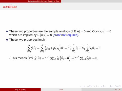
continue
These two properties are the sample analogs of E [u] = 0 and Cov (x ,u) = 0which are implied by E [ujx ] = 0 [proof not required].
These two properties imply
n
∑i=1
byibui =n
∑i=1
�bβ 0+bβ 1xi
�bui =bβ 0
n
∑i=1
bui +bβ 1
n
∑i=1
xibui = 0.
- This means dCov (by ,bu) = n�1 ∑ni=1 byi
�bui �bu�= n�1 ∑ni=1 byibui = 0.
Ping Yu (HKU) SLR 40 / 78
Properties of OLS on Any Sample of Data
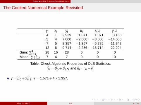
The Cooked Numerical Example Revisited
yi xi byi bui xibui byibui4 1 2.929 1.071 1.071 3.1385 4 7.000 �2.000 �8.000 �14.0007 5 8.357 �1.357 �6.785 �11.342
12 6 9.714 2.286 13.714 22.204Sum: ∑4
i=1 28 16 28 0 0 0Mean: 1
4 ∑4i=1 7 4 7 0 0 0
Table: Check Algebraic Properties of OLS Statistics:byi =bβ 0+
bβ 1xi and bui = yi �byi
y = bβ 0+ xbβ 1: 7= 1.571+4�1.357.
Ping Yu (HKU) SLR 41 / 78
Properties of OLS on Any Sample of Data
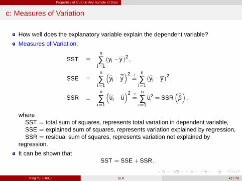
c: Measures of Variation
How well does the explanatory variable explain the dependent variable?
Measures of Variation:
SST �n
∑i=1(yi �y)2 ,
SSE �n
∑i=1
�byi �by�2 ?=
n
∑i=1(byi �y)2 ,
SSR �n
∑i=1
�bui �bu�2 ?=
n
∑i=1
bu2i = SSR
�bβ� ,where
SST = total sum of squares, represents total variation in dependent variable,SSE = explained sum of squares, represents variation explained by regression,SSR = residual sum of squares, represents variation not explained by
regression.
It can be shown thatSST = SSE +SSR.
Ping Yu (HKU) SLR 42 / 78
Properties of OLS on Any Sample of Data
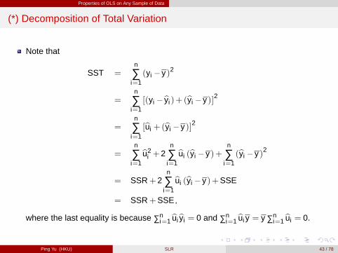
(*) Decomposition of Total Variation
Note that
SST =n
∑i=1(yi �y)2
=n
∑i=1[(yi �byi )+ (byi �y)]2
=n
∑i=1[bui +(byi �y)]2
=n
∑i=1
bu2i +2
n
∑i=1
bui (byi �y)+n
∑i=1(byi �y)2
= SSR+2n
∑i=1
bui (byi �y)+SSE
= SSR+SSE ,
where the last equality is because ∑ni=1 buibyi = 0 and ∑n
i=1 buiy = y ∑ni=1 bui = 0.
Ping Yu (HKU) SLR 43 / 78
Properties of OLS on Any Sample of Data
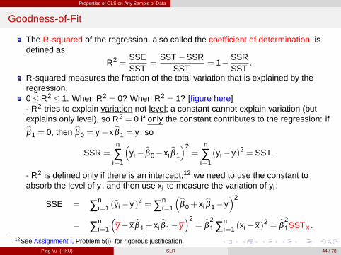
Goodness-of-Fit
The R-squared of the regression, also called the coefficient of determination, isdefined as
R2 =SSESST
=SST �SSR
SST= 1� SSR
SST.
R-squared measures the fraction of the total variation that is explained by theregression.0� R2 � 1. When R2 = 0? When R2 = 1? [figure here]- R2 tries to explain variation not level; a constant cannot explain variation (butexplains only level), so R2 = 0 if only the constant contributes to the regression: ifbβ 1 = 0, then bβ 0 = y �xbβ 1 = y , so
SSR =n
∑i=1
�yi � bβ 0�xi
bβ 1
�2=
n
∑i=1(yi �y)2 = SST .
- R2 is defined only if there is an intercept;12 we need to use the constant toabsorb the level of y , and then use xi to measure the variation of yi :
SSE = ∑ni=1 (byi �y)2 =∑n
i=1
�bβ 0+ xibβ 1�y
�2
= ∑ni=1
�y �xbβ 1+ xi
bβ 1�y�2= bβ 2
1 ∑ni=1 (xi �x)2 = bβ 2
1SST x .
12See Assignment I, Problem 5(i), for rigorous justification.Ping Yu (HKU) SLR 44 / 78
Properties of OLS on Any Sample of Data
0 0.2 0.4 0.6 0.8 12
1
0
2
3
4
0 0.2 0.4 0.6 0.8 11
1.1
1.2
1.3
1.4
1.5
1.6
1.7
1.8
1.9
2
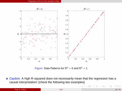
Figure: Data Patterns for R2 = 0 and R2 = 1
Caution: A high R-squared does not necessarily mean that the regression has acausal interpretation! [check the following two examples]
Ping Yu (HKU) SLR 45 / 78
Properties of OLS on Any Sample of Data
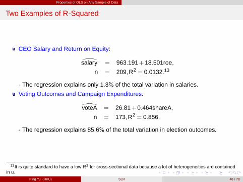
Two Examples of R-Squared
CEO Salary and Return on Equity:
\salary = 963.191+18.501roe,
n = 209,R2 = 0.0132.13
- The regression explains only 1.3% of the total variation in salaries.
Voting Outcomes and Campaign Expenditures:
\voteA = 26.81+0.464shareA,
n = 173,R2 = 0.856.
- The regression explains 85.6% of the total variation in election outcomes.
13It is quite standard to have a low R2 for cross-sectional data because a lot of heterogeneities are containedin u.
Ping Yu (HKU) SLR 46 / 78
Units of Measurement and Functional Form
Units of Measurement and Functional Form
Ping Yu (HKU) SLR 47 / 78
Units of Measurement and Functional Form
b: Incorporating Nonlinearities in Simple Regression
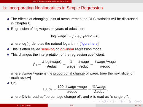
The effects of changing units of measurement on OLS statistics will be discussedin Chapter 6.
Regression of log wages on years of education:
log (wage) = β 0+β 1educ+u,
where log (�) denotes the natural logarithm. [figure here]
This is often called semi-log or log-linear regression model.
This changes the interpretation of the regression coefficient:
β 1 =∂ log (wage)
∂educ=
1wage
� ∂wage∂educ
=∂wage/wage
∂educ,
where ∂wage/wage is the proportional change of wage. [see the next slide formath review]
Or,
100β 1 =100 �∂wage/wage
∂educ=%∆wage
∆educ,
where %∆ is read as "percentage change of", and ∆ is read as "change of".
Ping Yu (HKU) SLR 48 / 78
Units of Measurement and Functional Form
[Review] Derivative of Logarithmic Functions
0 0.5 1 1.5 2 2.5 3 3.5 4 4.5 52
1.5
1
0.5
0
0.5
1
1.5
2
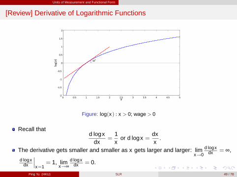
Figure: log(x) : x > 0; wage > 0
Recall thatd logx
dx=
1x
or d logx =dxx.
The derivative gets smaller and smaller as x gets larger and larger: limx!0
d logxdx = ∞,
d logxdx
���x=1
= 1, limx!∞
d logxdx = 0.
Ping Yu (HKU) SLR 49 / 78
Units of Measurement and Functional Form
A Log Wage Equation
The fitted regression line is
\log (wage) = 0.584+0.083educ,
n = 526,R2 = 0.186,
which implies\wage t e0.584+0.083educ .
The wage increases by 8.3% for every additional year of education (= return toeducation).
For example, if the current wage is $10 per hour (which implies that
educ = log(10)�0.5840.083 ), and suppose the education is increased by one year. Then
∆wage = exp�
0.584+0.083�
log(10)�0.5840.083
+1��
�10= 0.865t 0.83,
and∂wage/wage
∂educ=+$0.83/$10+1 year
= 0.083= 8.3%.
Ping Yu (HKU) SLR 50 / 78
Units of Measurement and Functional Form
0
1.793
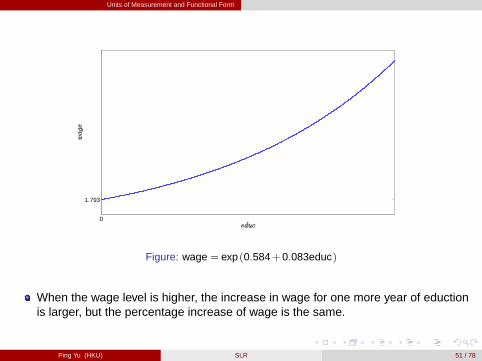
Figure: wage = exp (0.584+0.083educ)
When the wage level is higher, the increase in wage for one more year of eductionis larger, but the percentage increase of wage is the same.
Ping Yu (HKU) SLR 51 / 78
Units of Measurement and Functional Form
Constant Elasticity Model
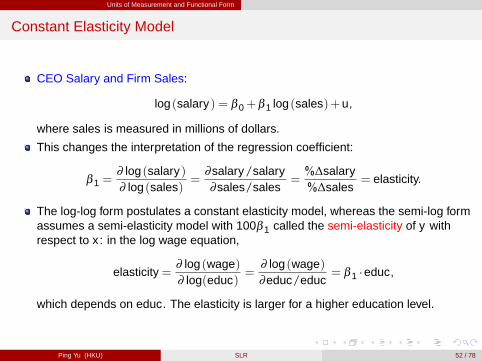
CEO Salary and Firm Sales:
log (salary) = β 0+β 1 log (sales)+u,
where sales is measured in millions of dollars.
This changes the interpretation of the regression coefficient:
β 1 =∂ log (salary)∂ log (sales)
=∂salary/salary∂sales/sales
=%∆salary%∆sales
= elasticity.
The log-log form postulates a constant elasticity model, whereas the semi-log formassumes a semi-elasticity model with 100β 1 called the semi-elasticity of y withrespect to x : in the log wage equation,
elasticity=∂ log (wage)∂ log(educ)
=∂ log (wage)∂educ/educ
= β 1 �educ,
which depends on educ. The elasticity is larger for a higher education level.
Ping Yu (HKU) SLR 52 / 78
Units of Measurement and Functional Form
CEO Salary and Firm Sales
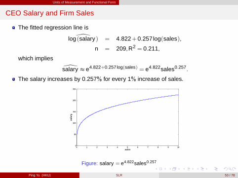
The fitted regression line is
\log (salary) = 4.822+0.257log(sales),
n = 209,R2 = 0.211,
which implies
\salary t e4.822+0.257log(sales) = e4.822sales0.257.
The salary increases by 0.257% for every 1% increase of sales.
0 1 2 3 4 5 6 7 8 9 100
50
100
150
200
250
Figure: salary = e4.822sales0.257
Ping Yu (HKU) SLR 53 / 78
Units of Measurement and Functional Form
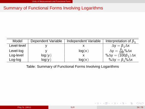
Summary of Functional Forms Involving Logarithms
Model Dependent Variable Independent Variable Interpretation of β 1Level-level y x ∆y = β 1∆x
Level-log y log(x) ∆y = β 1100%∆x
Log-level log (y) x %∆y = (100β 1)∆xLog-log log(y) log(x) %∆y = β 1%∆x
Table: Summary of Functional Forms Involving Logarithms
Ping Yu (HKU) SLR 54 / 78
Expected Values and Variances of the OLS Estimators
Expected Values and Variances of the OLS Estimators
Ping Yu (HKU) SLR 55 / 78
Expected Values and Variances of the OLS Estimators
Statistical Properties of OLS Estimators
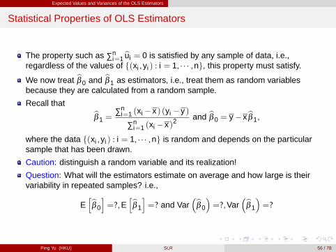
The property such as ∑ni=1 bui = 0 is satisfied by any sample of data, i.e.,
regardless of the values of f(xi ,yi ) : i = 1, � � � ,ng, this property must satisfy.
We now treat bβ 0 and bβ 1 as estimators, i.e., treat them as random variablesbecause they are calculated from a random sample.
Recall that bβ 1 =∑n
i=1 (xi �x) (yi �y)
∑ni=1 (xi �x)2
and bβ 0 = y �xbβ 1,
where the data f(xi ,yi ) : i = 1, � � � ,ng is random and depends on the particularsample that has been drawn.
Caution: distinguish a random variable and its realization!
Question: What will the estimators estimate on average and how large is theirvariability in repeated samples? i.e.,
Ehbβ 0
i=?,E
hbβ 1
i=? and Var
�bβ 0
�=?,Var
�bβ 1
�=?
Ping Yu (HKU) SLR 56 / 78
Expected Values and Variances of the OLS Estimators
Standard Assumptions for the SLR Model
Scientific approach requires assumptions! Science vs. Superstition
Assumption SLR.1 (Linear in Parameters):
y = β 0+β 1x +u.
- In the population, the relationship between y and x is linear.- The "linear" in linear regression means "linear in parameter", e.g.,y = β 0+β 1 log (x)+u is a linear regression.
Assumption SLR.2 (Random Sampling): The data f(xi ,yi ) : i = 1, � � � ,ng is arandom sample drawn from the population, i.e., each data point follows thepopulation equation,
yi = β 0+β 1xi +ui .
Ping Yu (HKU) SLR 57 / 78
Expected Values and Variances of the OLS Estimators
Discussion of Random Sampling: Wage and Education
The population consists, for example, of all workers of country A.
In the population, a linear relationship between wages (or log wages) and years ofeducation holds.
Draw completely randomly a worker from the population.
The wage and the years of education of the worker drawn are random becauseone does not know beforehand which worker is drawn.
Throw back worker into population and repeat random draw n times.
The wages and years of education of the sampled workers are used to estimatethe linear relationship between wages and education.
Ping Yu (HKU) SLR 58 / 78
Expected Values and Variances of the OLS Estimators
Figure: Graph of yi = β 0+β 1xi +ui .
Ping Yu (HKU) SLR 59 / 78
Expected Values and Variances of the OLS Estimators
continue
Assumption SLR.3 (Sample Variation in Explanatory Variable): ∑ni=1 (xi �x)2 > 0.
- The values of the explanatory variables are not all the same (otherwise it wouldbe impossible to study how much the dependent variable changes when theexplanatory variable changes one unit - β 1). [figure here]- Note that ∑n
i=1 (xi �x)2 is the demonimator of bβ 1. If ∑ni=1 (xi �x)2 = 0, then bβ 1 is
not defined.
Assumption SLR.4 (Zero Conditional Mean):
E [ui jxi ] = 0.
- The value of the explanatory variable must contain no information about themean of the unobserved factors.
Ping Yu (HKU) SLR 60 / 78
Expected Values and Variances of the OLS Estimators
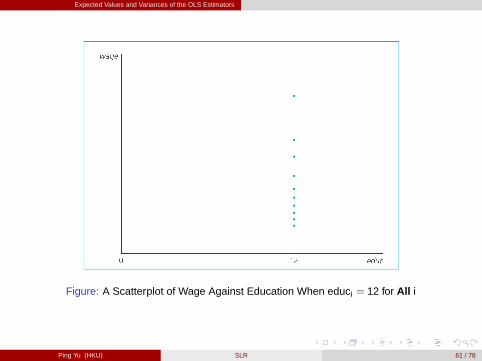
Figure: A Scatterplot of Wage Against Education When educi = 12 for All i
Ping Yu (HKU) SLR 61 / 78
Expected Values and Variances of the OLS Estimators
a: Unbiasedness of OLS
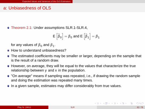
Theorem 2.1: Under assumptions SLR.1-SLR.4,
Ehbβ 0
i= β 0 and E
hbβ 1
i= β 1
for any values of β 0 and β 1.
How to understand unbiasedness?
The estimated coefficients may be smaller or larger, depending on the sample thatis the result of a random draw.
However, on average, they will be equal to the values that characterize the truerelationship between y and x in the population.
"On average" means if sampling was repeated, i.e., if drawing the random sampleand doing the estimation was repeated many times.
In a given sample, estimates may differ considerably from true values.
Ping Yu (HKU) SLR 62 / 78
Expected Values and Variances of the OLS Estimators
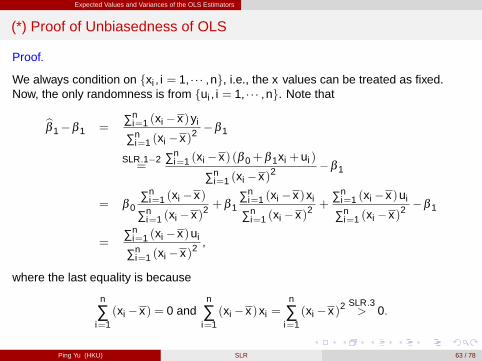
(*) Proof of Unbiasedness of OLS
Proof.
We always condition on fxi , i = 1, � � � ,ng, i.e., the x values can be treated as fixed.Now, the only randomness is from fui , i = 1, � � � ,ng. Note that
bβ 1�β 1 =∑n
i=1 (xi �x)yi
∑ni=1 (xi �x)2
�β 1
SLR.1�2=
∑ni=1 (xi �x) (β 0+β 1xi +ui )
∑ni=1 (xi �x)2
�β 1
= β 0∑n
i=1 (xi �x)
∑ni=1 (xi �x)2
+β 1∑n
i=1 (xi �x)xi
∑ni=1 (xi �x)2
+∑n
i=1 (xi �x)ui
∑ni=1 (xi �x)2
�β 1
=∑n
i=1 (xi �x)ui
∑ni=1 (xi �x)2
,
where the last equality is because
n
∑i=1(xi �x) = 0 and
n
∑i=1(xi �x)xi =
n
∑i=1(xi �x)2
SLR.3> 0.
Ping Yu (HKU) SLR 63 / 78
Expected Values and Variances of the OLS Estimators
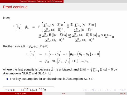
Proof continue
Now,
Ehbβ 1
i�β 1 = E
"∑n
i=1 (xi �x)ui
∑ni=1 (xi �x)2
#(ii)=
E�∑n
i=1 (xi �x)ui�
∑ni=1 (xi �x)2
(i)=
∑ni=1 E [(xi �x)ui ]
∑ni=1 (xi �x)2
(ii)=
∑ni=1 (xi �x)E [ui ]
∑ni=1 (xi �x)2
14 SLR.2�4= 0.
Further, since y = β 0+β 1x +u,
Ehbβ 0
i= E
hy �xbβ 1
i= E
hβ 0�
�bβ 1�β 1
�x +u
i= β 0�xE
hbβ 1�β 1
i+E [u] = β 0,
where the last equality is because bβ 1 is unbiased, and E [u] = 1n ∑n
i=1 E [ui ] = 0 byAssumptions SLR.2 and SLR.4. �
The key assumption for unbiasedness is Assumption SLR.4.
14E [ui jx1, � � � ,xn ]SLR.2= E [ui jxi ]
SLR.4= 0.
Ping Yu (HKU) SLR 64 / 78
Expected Values and Variances of the OLS Estimators
b: Variances of the OLS Estimators
Unbiasedness is not the only desirable property of the OLS estimator. [intuitionhere: gunfire][figure here]
Depending on the sample, the estimates will be nearer or farther away from thetrue population values.
How far can we expect our estimates to be away from the true population valueson average (= sampling variability)?
Sampling variability is measured by the estimator’s variances. [see the next slidesfor review of variance]
Ping Yu (HKU) SLR 65 / 78
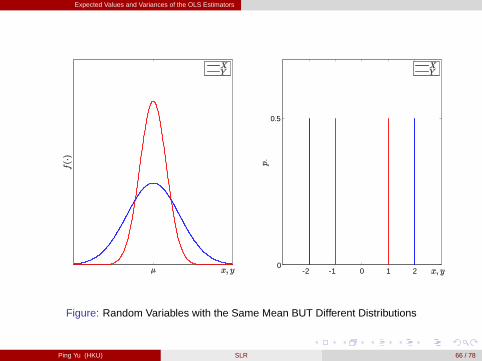
Expected Values and Variances of the OLS Estimators
2 1 0 1 20
0.5
Figure: Random Variables with the Same Mean BUT Different Distributions
Ping Yu (HKU) SLR 66 / 78
Expected Values and Variances of the OLS Estimators
[Review] Variance
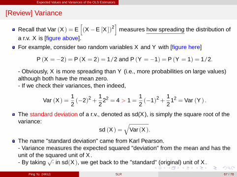
Recall that Var (X ) = Eh(X �E [X ])2
imeasures how spreading the distribution of
a r.v. X is [figure above].
For example, consider two random variables X and Y with [figure here]
P (X = �2) = P (X = 2) = 1/2 and P (Y = �1) = P (Y = 1) = 1/2.
- Obviously, X is more spreading than Y (i.e., more probabilities on large values)although both have the mean zero.- If we check their variances, then indeed,
Var (X ) =12(�2)2+
12
22 = 4 > 1=12(�1)2+
12
12 = Var (Y ) .
The standard deviation of a r.v., denoted as sd(X ), is simply the square root of thevariance:
sd (X ) =q
Var (X ).
The name "standard deviation" came from Karl Pearson.- Variance measures the expected squared "deviation" from the mean and has theunit of the squared unit of X .- By taking
p� in sd(X ), we get back to the "standard" (original) unit of X .
Ping Yu (HKU) SLR 67 / 78
Expected Values and Variances of the OLS Estimators
continue
If X = 1(college graduate), then Var (X ) = p (1�p)2+(1�p)(0�p)2 = p(1�p).[intuition here]
If X � N�
µ,σ2�
, then Var (X ) = σ2.
Two Useful Properties: (i) for independent r.v.’s, "the variance of the sum is thesum of the variances",
Var�∑n
i=1 Xi
�=∑n
i=1 Var (Xi ) ;
(ii) for any constants a and b, Var (a+bX ) = b2Var (X ).
- Var (a+bX ) = Eh(a+bX �a�bE [X ])2
i= b2E
h(X �E [X ])2
i= b2Var (X ) .
These two properties imply
Var (x) = Var
1n
n
∑i=1
xi
!(ii)=
1n2 Var
n
∑i=1
xi
!SLR.2+(i)=
1n2
n
∑i=1
Var (xi )SLR.2=
nVar (x)n2 =
Var (x)n
,
which decreases with n and increases with Var (x).
Ping Yu (HKU) SLR 68 / 78
Expected Values and Variances of the OLS Estimators
[Review] Conditional Variance
As the conditional mean, the conditional variance of Y given X = x , denoted asVar (Y jX = x), is the variance of Y for the (slice of) individuals with X = x .Rigorously,
Var (Y jX = x) = Eh(Y �E [Y jX = x ])2 jX = x
i.
Apply the second property of variance to the conditional variance to have
Var (yi jxi ) = Var (yi �β 0�β 1xi jxi ) = Var (ui jxi ) ,
where as mentioned in the conditional mean, conditional on xi , β 0+β 1xi can betreated as a constant like a in (ii).
Although E [yi jxi ] = β 0+β 1xi is linear in xi (Assumption SLR1, 2 and 4),Var (yi jxi ) is assumed not to depend on xi (Assumption SLR.5 below).
Ping Yu (HKU) SLR 69 / 78
Expected Values and Variances of the OLS Estimators
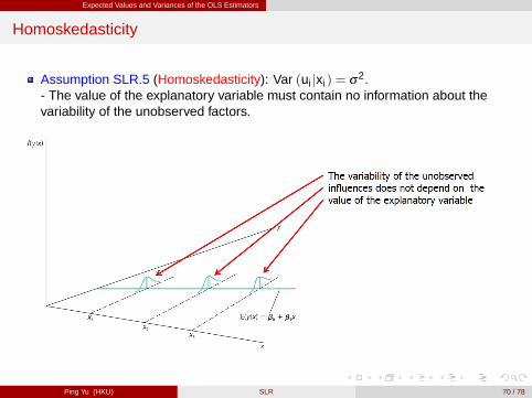
Homoskedasticity
Assumption SLR.5 (Homoskedasticity): Var (ui jxi ) = σ2.- The value of the explanatory variable must contain no information about thevariability of the unobserved factors.
Ping Yu (HKU) SLR 70 / 78
Expected Values and Variances of the OLS Estimators
Heteroskedasticity
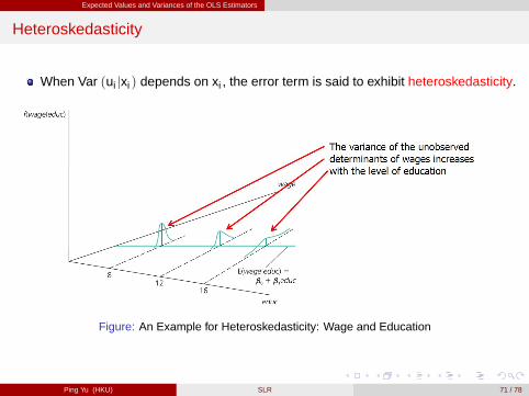
When Var (ui jxi ) depends on xi , the error term is said to exhibit heteroskedasticity.
Figure: An Example for Heteroskedasticity: Wage and Education
Ping Yu (HKU) SLR 71 / 78
Expected Values and Variances of the OLS Estimators
Variances of OLS Estimators
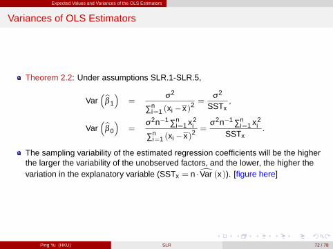
Theorem 2.2: Under assumptions SLR.1-SLR.5,
Var�bβ 1
�=
σ2
∑ni=1 (xi �x)2
=σ2
SSTx,
Var�bβ 0
�=
σ2n�1 ∑ni=1 x2
i
∑ni=1 (xi �x)2
=σ2n�1 ∑n
i=1 x2i
SSTx.
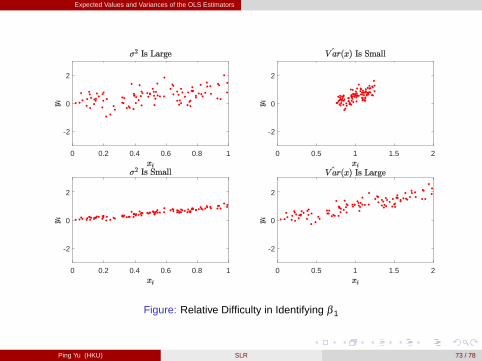
The sampling variability of the estimated regression coefficients will be the higherthe larger the variability of the unobserved factors, and the lower, the higher thevariation in the explanatory variable (SSTx = n �dVar (x)). [figure here]
Ping Yu (HKU) SLR 72 / 78
Expected Values and Variances of the OLS Estimators
0 0.2 0.4 0.6 0.8 1
2
0
2
0 0.2 0.4 0.6 0.8 1
2
0
2
0 0.5 1 1.5 2
2
0
2
0 0.5 1 1.5 2
2
0
2
Figure: Relative Difficulty in Identifying β 1
Ping Yu (HKU) SLR 73 / 78
Expected Values and Variances of the OLS Estimators
(*) Proof of Theorem 2.2
Proof.
Var�bβ 1
�is more important, so we concentrate on it here. As in the proof of Theorem
2.1, we condition on fxi , i = 1, � � � ,ng.
Var�bβ 1
�(ii)15
= Var�bβ 1�β 1
�= Var
�∑n
i=1(xi�x)ui
∑ni=1(xi�x)2
�(ii)=
Var (∑ni=1(xi�x)ui )SST 2
x
SLR.2+(i)= ∑n
i=1 Var ((xi�x)ui )SST 2
x(ii)= ∑n
i=1(xi�x)2Var (ui )SST 2
x
16 SLR.2+5= ∑n
i=1(xi�x)2σ2
SST 2x
= σ2SSTxSST 2
x= σ2
SSTx.
�The key assumption to get this simple formula of Var
�bβ 1
�is Assumption SLR.5.
The only unknown component of Var�bβ 1
�and Var
�bβ 0
�is σ2 which is estimated
below.
15Also because Ehbβ 1
i= β 1 and we want to "center" bβ 1 at zero.
16Var (ui jx1, � � � ,xn)SLR.2= Var (ui jxi )
SLR.5= σ2.
Ping Yu (HKU) SLR 74 / 78
Expected Values and Variances of the OLS Estimators
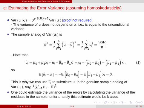
c: Estimating the Error Variance (assuming homoskedasticity)
Var (ui jxi ) = σ2 SLR.4+5= Var (ui ) [proof not required].
- The variance of u does not depend on x , i.e., is equal to the unconditionalvariance.
The sample analog of Var (ui ) is
eσ2 =1n
n
∑i=1
�bui �bu�2=
1n
n
∑i=1
bu2i =
SSRn.
- Note that
bui = β 0+β 1xi +ui � bβ 0� bβ 1xi = ui ��bβ 0�β 0
���bβ 1�β 1
�xi , (1)
soE [bui �ui ] = �E
hbβ 0�β 0
i�E
hbβ 1�β 1
ixi = 0.
This is why we can use bui to substitute ui in the genuine sample analog ofVar (ui ), say, 1
n ∑ni=1 (ui �u)2.
One could estimate the variance of the errors by calculating the variance of theresiduals in the sample; unfortunately this estimate would be biased .
Ping Yu (HKU) SLR 75 / 78
Expected Values and Variances of the OLS Estimators
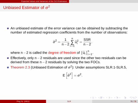
Unbiased Estimator of σ2
An unbiased estimate of the error variance can be obtained by subtracting thenumber of estimated regression coefficients from the number of observations:
bσ2 =1
n�2
n
∑i=1
bu2i =
SSRn�2
.
where n�2 is called the degree of freedom of�buin
i=1.
Effectively, only n�2 residuals are used since the other two residuals can bederived from these n�2 residuals by solving the two FOCs.
Theorem 2.3 (Unbiased Estimation of σ2): Under assumptions SLR.1-SLR.5,
Ehbσ2
i= σ
2.
Ping Yu (HKU) SLR 76 / 78
Expected Values and Variances of the OLS Estimators
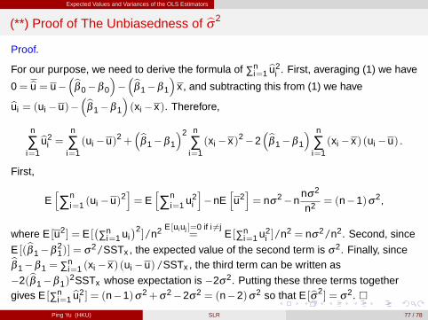
(**) Proof of The Unbiasedness of bσ2
Proof.
For our purpose, we need to derive the formula of ∑ni=1 bu2
i . First, averaging (1) we have
0= bu = u��bβ 0�β 0
���bβ 1�β 1
�x , and subtracting this from (1) we havebui = (ui �u)�
�bβ 1�β 1
�(xi �x). Therefore,
n
∑i=1
bu2i =
n
∑i=1(ui �u)2+
�bβ 1�β 1
�2 n
∑i=1(xi �x)2�2
�bβ 1�β 1
� n
∑i=1(xi �x) (ui �u) .
First,
Eh∑n
i=1 (ui �u)2i= E
h∑n
i=1 u2i
i�nE
hu2i= nσ
2�nnσ2
n2 = (n�1)σ2,
where E [u2] = E [�∑n
i=1 ui�2]/n2 E [ui uj ]=0 if i 6=j
= E [∑ni=1 u2
i ]/n2 = nσ2/n2. Second, since
E [(bβ 1�β21)] = σ2/SSTx , the expected value of the second term is σ2. Finally, sincebβ 1�β 1 = ∑n
i=1 (xi �x) (ui �u)/SSTx , the third term can be written as
�2(bβ 1�β 1)2SSTx whose expectation is �2σ2. Putting these three terms together
gives E [∑ni=1 bu2
i ] = (n�1)σ2+σ2�2σ2 = (n�2)σ2 so that E [bσ2] = σ2. �Ping Yu (HKU) SLR 77 / 78
Expected Values and Variances of the OLS Estimators
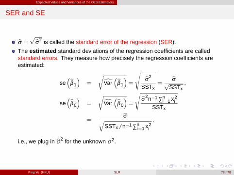
SER and SE
bσ =pbσ2 is called the standard error of the regression (SER).
The estimated standard deviations of the regression coefficients are calledstandard errors. They measure how precisely the regression coefficients areestimated:
se�bβ 1
�=
rdVar�bβ 1
�=
s bσ2
SSTx=
bσpSSTx
,
se�bβ 0
�=
rdVar�bβ 0
�=
sbσ2n�1 ∑ni=1 x2
iSSTx
=bσq
SSTx /n�1 ∑ni=1 x2
i
,
i.e., we plug in bσ2 for the unknown σ2.
Ping Yu (HKU) SLR 78 / 78


