ARTICLE IN PRESS

Contents lists available at ScienceDirect

Acta Astronautica

Acta Astronautica ] (]]]]) ]]]–]]]

0094-57

doi:10.1

� Cor

E-m

(G.C. Ru

PleasAstro

journal homepage: www.elsevier.com/locate/actaastro

CFD rebuilding of USV-DTFT1 vehicle in-flight experiment

Pietro Roncioni �, Giuseppe C. Rufolo, Marco Marini, Salvatore Borrelli

CIRA, Italian Aerospace Research Centre, 81043 Capua, Italy

a r t i c l e i n f o

Article history:

Received 27 January 2009

Received in revised form

13 October 2009

Accepted 13 October 2009

Keywords:

PRO.R.A.-USV FTB-1 vehicle

In-flight experiment

CFD rebuilding

65/$ - see front matter & 2009 Elsevier Ltd. A

016/j.actaastro.2009.10.015

responding author. Tel.: þ390823623035; fax

ail addresses: p.roncioni@cira.it (P. Roncioni),

folo), m.marini@cira.it (M. Marini), s.borrelli@

e cite this article as: P. Roncioninautica (2009), doi:10.1016/j.actaas

a b s t r a c t

The aim of this paper is to present some numerical rebuilding results of the in-flight

aerodynamic experiment carried out during the first mission Dropped Transonic Flight

Test (DTFT) of the Italian Aerospace Research Centre (CIRA) Unmanned Space Vehicle

(USV). USV is a multi-mission, re-usable vehicle developed at CIRA and it is funded by

the Italian National Aerospace Research Program (PRO.R.A.). The first mission was

performed at the end of February 2007, and it was aimed at experimenting the transonic

flight of a re-entry vehicle. One of the aims of the aerodynamic experiment is the

validation and improvement of the prediction tools (CFD, extrapolation to flight)

through the comparison between pre-flight predictions and in-flight measured data.

Some selected flight conditions occurred during the DTFT mission have been

numerically rebuilt aimed at reproducing the most relevant fluid dynamic phenomena

characterizing the USV vehicle aerodynamics. The analysis of numerically rebuilt flight

conditions has allowed the assessment of local non-linear phenomenologies and,

depending on both the analysis of the numerical results and the comparison with the

flight data, an assessment of the entire CFD methodology.

& 2009 Elsevier Ltd. All rights reserved.

1. Introduction

The CIRA USV (Unmanned Space Vehicle) is a multi-mission, re-usable vehicle developed at CIRA, the ItalianAerospace Research Centre, and it is funded by the ItalianNational Aerospace Research Program, i.e. the PRO.R.A.[1]. It is basically a slender, not-propelled, winged vehicleable to perform experiments on aerodynamics, structureand materials, autonomous guidance navigation andcontrol. The aim of this work is to present some numericalrebuilding results of the in-flight aerodynamic experi-ment carried out during the first mission DTFT (DroppedTransonic Flight Test).

This first mission was performed on February 24th,2007 from the base of Arbatax in Sardinia, Italy, and it was

ll rights reserved.

: þ390823623700.

g.rufolo@cira.it

cira.it (S. Borrelli).

, et al., CFD rebuildtro.2009.10.015

aimed at experimenting the transonic flight of a re-entryvehicle [2].

The aerodynamic characterization of the transonicphase of a re-entry space vehicle trajectory is criticaldue to the strong variability of the aerodynamic coeffi-cients, the reason being the non-linear behaviour of theflow field. In this framework, it is really importantto correctly predict the aerodynamic performance ofthe vehicle by means of suitably developed CFD tools. Oneof the aims of the aerodynamic experiment is thevalidation and improvement of the prediction tools(CFD, methodology of extrapolation-to-flight) throughthe comparison between pre-flight predictions and in-flight measurements.

Both global aerodynamic coefficients (inertial measure-ments) and local quantities (pressure measurements) havebeen acquired during the flight [2]. In order to compare localpressure distributions and global aerodynamic coefficientssome selected flight conditions of the DTFT mission havebeen numerically rebuilt aimed at reproducing the mostrelevant fluid dynamic phenomena characterizing the USV

ing of USV-DTFT1 vehicle in-flight experiment, Acta

ARTICLE IN PRESS

Nomenclature

AoA, a angle of attackAoS, b sideslip angleCD drag coefficientCL lift coefficientCY side force coefficientCp pressure coefficientCl roll coefficientCm pitching coefficient

Cn yaw coefficientCoM centre of massk–e two-equation turbulence modellingM Mach numberpw surface pressureRe Reynolds numberXcp position of centre of pressureX, Y, Z spatial coordinatesdR;L

E elevon deflection angle

dR;LR rudder deflection angle

P. Roncioni et al. / Acta Astronautica ] (]]]]) ]]]–]]]2

vehicle’s aerodynamics. Early results are reported in Refs.[3,4], while recent improvements and additional computa-tions are reported in the present paper.

The numerical CFD simulations (both Eulerian andviscous turbulent CFD computations) have been carriedout by means of the CIRA code H3NS [5], a RANSmultiblock finite volume solver based on a Flux DifferenceSplitting second order numerical scheme. The k–e1

Myong-Kasagi turbulence modelling [6] has been usedfor turbulent viscous simulations.

From CFD computations both global aerodynamiccoefficients and local pressure distributions can beextracted, thus allowing for the comparison of CFD resultswith the in-flight acquired global forces and moments andstatic pressure measurements. The analysis of numericallyrebuilt flight conditions allowed the assessment of localnon-linear phenomenologies, such as separation inducedby shock waves and flap deflection and the highsensitivity of shock position with the Mach number, aswell as a better understanding of the global aerodynamiccoefficients behaviours as function of both Mach numberand angle of attack.

2. The DTFT-1 mission

The USV FTB-1 vehicle will perform several missions,each of them with an increasing maximum Mach number(up to about 2), aimed at simulating the final portion of atypical re-entry trajectory [2]. USV FTB-1 vehicle isbasically composed by a Flying Test Bed (the FTB-1vehicle) and a carrier based on a stratospheric balloon.During the missions the balloon carries the FTB-1 up tothe desired altitude and then, after having established acruise horizontal trajectory, releases it from the gondola.At this moment the FTB-1 vehicle starts its own flightfollowing the designed trajectory. The theoretical limit ofthe envelope of possible missions (i.e. what is commonlycalled ‘‘flight corridor’’) is mainly due to the performanceof the stratospheric balloon used as a carrier [2,4].

For the first USV FTB-1 mission the vehicle has beenreleased from an altitude of about 20 Km with the aim atexperimenting the transonic flight of a re-entry vehicle(see Fig. 1). In particular, the objective of the experimentperformed during this first mission has been the

1 See Nomenclature at end of paper.

Please cite this article as: P. Roncioni, et al., CFD rebuildAstronautica (2009), doi:10.1016/j.actaastro.2009.10.015

evaluation of the effect of a Mach number sweep, atnearly constant angle-of-attack, on the longitudinal globalaerodynamic coefficients (sideslip angle of the mission isnominally zero).

More details about the second DTFT mission (max-imum Mach number 1.2 and a-sweep at constant Mach)and the third, and final, Dropped Supersonic Flight Test(DSFT mission) of FTB-1 vehicle (an extension ofthe second DTFT mission to about Mach 2) are given inRef. [4].

3. The FTB-1 vehicle

The FTB-1 vehicle is a winged body (see Fig. 2) with anoverall length of 8 m and a total weight of about 1350 kg.The windside part of the front fuselage (characterized by a1 cm radius hemispheric quasi-conical nose) rapidlychanges from a quasi-circular to a rounded-squaresection shape. The mid-fuselage is characterized by aquasi-constant section while the afterbody ends with aboat-tailed truncated base. The wing of the FTB-1 vehiclehas a double delta shape with a main 451 sweepbackleading edge and a strake with a 761 sweepback leadingedge. The trailing edge has a sweepforward angle of 61. Toimprove the vehicle’s lateral stability, the wing has adihedral angle of 51. Overall wing span is 3.562 m, whilethe strake root chord is 2.82 m. An elevon with both thefunctions of elevator and aileron is mounted on the wing.

To allow directional stability and control two verticaltails have been adopted, with a dihedral angle of 401, asweepback angle of 451 and a span of 0.8 m. A pair of full-span movable rudders is also implemented for the controlof directionality.

Moreover, in order to augment directional stabilitycharacteristics of the vehicle and to reduce possibilities ofDutch-Roll occurrence, a pair of full symmetric ventralfins has been added. These fixed fins are characterized bya 551 sweepback angle, a root chord of 0.8 m with a taperratio of 0.455, and a span of 0.418 m. They have beenconceived in order to have the highest effectiveness withthe lowest impact on structure.

4. Pre-flight activities

A short description of the pre-flight activitiesconcerning both the aerodynamic database development

ing of USV-DTFT1 vehicle in-flight experiment, Acta

ARTICLE IN PRESS

0 0.2 0.4 0.6 0.8 1

1

1.2

1.4

1.6

1.8

2

x 104

Mach Number

Alti

tude

[m]

Mach-h Plot

4.5 g Parachute LimitTarget AreaSensor Limits

Mach 0.7 @ 21 s

Mach 1 @ 35 s

End Mission @ 39.39 s

Sensor Calibration Zone

Fig. 1. USV FTB-1 DTFT-1 mission.

Fig. 2. USV FTB-1 vehicle.

P. Roncioni et al. / Acta Astronautica ] (]]]]) ]]]–]]] 3

and the in-flight aerodynamic experiment set-up is givenhereinafter.

4.1. Aero-Data-Base (ADB)

The aerodynamic characteristics of the USV FTB-1winged vehicle are described by means of a suitablydeveloped Aerodynamic Prediction Model (APM), see Ref.[7]. The six global aerodynamic coefficients (CL, CD, CY : lift,drag and side forces; Cl, Cm, Cn : rolling, pitching andyawing moments), the hinge moments ðCi

HÞ of the controldevices (elevons, rudders) and the surface pressuredistribution (pw) have been fully characterized in theAPM.

The classical build-up approach [8–10] has been usedfor the description of the global aerodynamic coefficients,where each coefficient is expressed as a linear summationover a certain number of contributions, each of themdependent by a small number of parameters. In general,each global aerodynamic coefficient is expressed as thesum of a baseline contribution (at zero-sideslip, in cleanconfiguration and with no dynamic effects) and of a

Please cite this article as: P. Roncioni, et al., CFD rebuildAstronautica (2009), doi:10.1016/j.actaastro.2009.10.015

number of delta coefficients describing the effects ofthe different (independent) parameters on the baselinevalue [7].

The experimental data needed to explicit the func-tional expressions of the APM have been mainly gatheredin two different wind tunnel test campaign: the firstcarried out at the CIRA PT-1 Transonic Wind Tunnel [11],and the second one at the Transonic Wind TunnelGottingen (TWG) of DNW consortium [12,13]. In thiscontext CFD simulations have been used both to cross-check wind tunnel data and to fill measurements gaps(estimation of base drag, Reynolds number effect andmodel support system interference), and finally they havebeen useful to achieve a deeper understanding of theentire vehicle’s aerodynamics. In addition, simplifiednumerical methods like Eulerian CFD, Vortex LatticeMethod, Panel Method and DATCOM have been used tofill existing gaps in wind tunnel data for Mo0.5, toprovide a rapid estimation of configuration changesoccurring during the design process, and mainly toprovide dynamic stability derivatives [7].

Even though the aerodynamic prediction model isaimed at being the best possible by exploiting theavailable tools and know-how, it remains, however, onlya representation of the actual phenomenology, andtherefore it is characterized by errors. To assess the APMoutput data it is then necessary to estimate the entity ofsuch errors, by associating to the nominal values therelative uncertainty margins. The uncertainty modelassociated to the present APM is characterized by aproper functional structure, and by a certain number ofbasic parameters [14]. Each uncertainty has been obtainedas a summation of different contributions due to thedifferent parts of the APM (WT, CFD). Namely, for the

ing of USV-DTFT1 vehicle in-flight experiment, Acta

ARTICLE IN PRESS

P. Roncioni et al. / Acta Astronautica ] (]]]]) ]]]–]]]4

wind tunnel data, used as core for the APM, two differentkinds of uncertainties have been considered: randomexperimental error (repeatability); systematic experimen-tal errors (known and not removable errors) as forinstance the error of the balance used for forces andmoments measurements, the error in the calibration ofthe test section, the error in the positioning of the modelsupport system. Following the common practice adoptedfor WT measurements [17] a quadratic summation rulehas been adopted for these uncertainty contributions. Forwhat concern the CFD data, used to extrapolate to flightconditions the WT data, and following the classicaltaxonomy adopted for CFD [18], it is possible to recognizethese error sources: iteration error (convergence criter-ion), discretization error (grid independence, algorithmerror), modelling error (initial and boundary conditions,geometry representation, turbulence model). Apart fromthe first two of these error which meaning is straightfor-ward and that will be recalled in the following paragraph,the modelling error has been evaluated on the basis ofvalidation activities (measurement-to-prediction uncer-tainty) performed on the CIRA numerical code withrespect to wind tunnel experimental measurement. Inorder to be conservative a linear rule has been assumed toadd experimental and CFD uncertainties. To these errors,that are to some extent traceable, it has been added theuncertainty related to the so called unknown unknowns,i.e. the uncertainty due to the lack of knowledge withrespect to unexpected fluid flow phenomenology occur-ring during flight. The estimation of this latter uncertaintycontribution is by far the most complicated and priorto the execution of flight test it can only be based onpast experience relative to space vehicle of similar type(e.g. Space shuttle).

4.2. In-flight aerodynamic experiment

The main target of the aerodynamic in-flight experi-ment has been to provide a database of global (forces,moments) and local (static pressures) measurements

Fig. 3. Pressure coefficient contours

Please cite this article as: P. Roncioni, et al., CFD rebuildAstronautica (2009), doi:10.1016/j.actaastro.2009.10.015

useful to support and improve the CFD tools employedfor the vehicle’s design [3].

The aerodynamic forces and moments are derivedstarting from measurements of vehicle’s accelerations andattitude during flight. On the other hand, the set-up of theexperiment for the measurement of surface pressureduring flight is shortly described in this section majordetails can be found in Ref. [3].

A deep analysis of surface pressure distributionobtained by means of pre-flight CFD simulations fordifferent flight conditions (M=0.7, 0.94, 1.05; a=0,101)has allowed to identify the most interesting regions interms of maximum gradients and maximum variationswith respect to Mach number and vehicle attitude. Fig. 3reports the locations of pressure probes superimposed tothe CFD-predicted pressure coefficient field at M=1.05and a=101.

An overall number of 304 pressure taps has beenselected for the aerodynamic in-flight experiment. Datahave been acquired up to 39 s from release with afrequency of 10 Hz.

In particular, the attention has been focused on thefollowing regions (see Fig. 3): the nose, with the aim atstudying a flush mounted Air Data System (ADS); thewing, the lifting surface with the maximum pressurevariation and presence of shock waves in transonicregime; the mid and rear fuselage characterised, respec-tively, by large pressure variations in non-symmetricflight conditions and strong interference caused by theupper and lower vertical tails; the base, with an extendedre-circulating flow region, thus causing many difficultiesfor numerical prediction.

5. CFD numerical rebuilding

5.1. Trajectory points selection

Present numerical simulations are aimed at reprodu-cing the most relevant fluid dynamic phenomena char-acterizing the USV FTB-1 vehicle aerodynamics. Lookingat the flown flight trajectory, five conditions have been

with pressure taps positions.

ing of USV-DTFT1 vehicle in-flight experiment, Acta

ARTICLE IN PRESS

Table 1Trajectory points selected for CFD simulations.

Time (s) AoA (1) AoS (1) Mach (–) ReyL=1.05 (–) dER (1) dEL (1) dRR (1) dRL (1)

21.5 5.410 0.20 0.6997 1900214 �0.79 �0.36 1.26 1.22

28.8 6.456 �0.34 0.9051 3208178 �2.74 �3.04 0.79 0.70

30.8 6.564 �0.78 0.9496 3630894 �2.33 �3.95 0.39 0.32

31.3 5.390 �0.70 0.9606 3741757 �4.96 �6.20 0.11 0.02

36.6 6.405 0.00 1.0353 4984582 �9.87 �10.26 �0.58 �0.65

Fig. 4. Angle of attack versus time: red vertical lines indicate flight instants selected for CFD simulations.

P. Roncioni et al. / Acta Astronautica ] (]]]]) ]]]–]]] 5

selected and reported in Table 1 in terms of time elapsedfrom release, Mach and Reynolds numbers, angle ofattack, angle of sideslip and control surfaces deflections.In Fig. 4, where the angle of attack measured along thetrajectory versus time is reported, the flight conditionsselected to be rebuilt are indicated with red lines.

Both Eulerian and viscous turbulent CFD simulationshave been carried out for the selected points, byconsidering air as an ideal gas.

5.2. CFD code: H3NS

The numerical methodology used to carry out theaerodynamic analysis of the USV FTB-1 vehicle is based onthe CIRA code H3NS, developed and validated by theLaboratory of Aerothermodynamics and Space Propulsion[5]. It solves the Reynolds Average Navier–Stokes equa-tions in a density-based finite volume approach with a cellcentred Flux Difference Splitting second order ENO-likeupwind scheme for the convective terms. Viscous fluxesare computed with a classical centred scheme. Timeintegration is performed by employing an explicit multi-stage Runge–Kutta algorithm coupled with an implicitevaluation of source terms.

Working gas is air that can be properly modelled inthe hypothesis of ideal gas, equilibrium gas and thermo-chemical non-equilibrium gas. Moreover, several two-equation k2e turbulence models can be used for eddyviscosity calculation. Present simulations have beenperformed by using the standard k2e Myong–Kasagiturbulence model [6], without compressibility corrections.

Please cite this article as: P. Roncioni, et al., CFD rebuildAstronautica (2009), doi:10.1016/j.actaastro.2009.10.015

In this method particular damping functions are introducedto simulate the behaviour of the flow in the viscous regionof a turbulent boundary layer.

5.3. Computational grids and grid convergence

Several multi-block structured grids have been gener-ated by using the commercial software package ANSYSICEMCFDs-HEXA. The O-Grid block decomposition tech-nique has been used in order to have mesh blockswrapping the vehicle and with a direction outgoing fromthe body wall, necessary for the boundary layer stretch-ing. An example of surface grid over the vehicle and gridon the symmetry plane is shown in Fig. 5.

The far-field surfaces of the half-body grid (in thehypothesis of zero side-slip) have been located at aboutten body-lengths far from the body. Since the goal of thenumerical simulations is to rebuild some relevant condi-tions of the flown trajectory, a grid for each of thesepoints, characterized by a different control surfacedeflection (see Table 1), has been generated. The gapsboth along chord-wise and span-wise directions betweenthe elevon (right part of the vehicle only) and the wing/fuselage part have not been considered. The resultingwedge topology has been meshed by using collapsed facesat wall, properly treated by the CFD code H3NS.

The final computational grids are composed by 146blocks and about 3 millions of cells for the Eulerianversion, and 4.4 millions of cells for the viscous one.

It is very important, when dealing with a numericalsolution, to be confident about its reliability. Stated that

ing of USV-DTFT1 vehicle in-flight experiment, Acta

ARTICLE IN PRESS

Fig. 5. FTB-1 transonic grid.

P. Roncioni et al. / Acta Astronautica ] (]]]]) ]]]–]]]6

the code we are using has been validated in previoussteps, by comparison of numerical results and (windtunnel) experimental measurements, and so that themathematical model, numerically resolved, is representa-tive of the real world, each time we use the code we needto be sure that the numerical solution is the ‘‘exact’’solution of the mathematical model applied to theparticular problem we are working on. In order to do thiswe need to eliminate (from a theoretical point of view) orat least to bound (from a practical point of view) the timeconvergence (iteration) error and the grid convergenceerror. This step is known as verification [15,18] andconcerns only the problem of finding a mathematical/numerical solution of a given set of partial differentialequations. For what concerns the iteration error, it has tobe said that, especially when the flow field to be resolvedcontains features characterized by intrinsic unsteadiness(e.g. recirculation bubble, vortex shedding, base flow), theresidual of the equations does not decrease towards themachine precision. Despite the presence of these unstea-diness, the quantities of interest in our case, as globalaerodynamic coefficients and the pressure distributionsover the wing, reach a steady state value so that theiteration error can be neglected. On the other hand thegrid error, due to the use of a finite number of cells, cannotbe neglected and has to be estimated by means of a gridsensitivity analysis. This latter [3] has been carried out, forthe present study, at M=0.94, a=7.241, b=01 and dR

E ¼

�2:433 by using three levels of the structured multiblockgrid. The number of cells of the finest level (L3) isrespectively 8 and 64 times the one of the medium (L2)and the coarse (L1) levels.

Please cite this article as: P. Roncioni, et al., CFD rebuildAstronautica (2009), doi:10.1016/j.actaastro.2009.10.015

The trend of global aerodynamic coefficients versus theinverse of the cubic root of the number of cells(representative of the degree of grid resolution) is in theasymptotic range of convergence (see Fig. 6 for the liftcoefficient). In this way it is possible to use the Richardsonextrapolation theory [15,16] to obtain higher order valuesfor the global coefficients and above all a contribution tothe whole uncertainty levels due to the grid dependenceof global aerodynamic coefficients. The error bars of theL2–L3 and L1–L2 Richardson extrapolated values, asobtained with the above said theory, are reported in thegrid convergence plots (Fig. 6). It is interesting to noteas the L2–L3 (fine) error bar is fully contained within theL1–L2 (coarse) one. Similar considerations can be donefor grid convergence of Drag and Pitching momentcoefficients. A local grid convergence can be observedalso from Fig. 7, where the chord-wise pressure coefficientdistribution is reported, for the analysed flight condition,at the Y=1.0 m wing section. The asymptotic range ofconvergence has been nearly reached for all the positions.However, it has to be said that the level of gridconvergence is not equal for all the parameters and thatthe number of cells we choose depends on the type ofsimulations we are working on and in particular on theresults we expect from.

5.4. Comparison between CFD results and flight experiment:

static pressures

In this section an analysis of the numerical results anda comparison with the flight experiments is given. As said

ing of USV-DTFT1 vehicle in-flight experiment, Acta

ARTICLE IN PRESS

M=0.94, AoA=7.24°, AoS=0°, δ_δ_E_R=-2.43°

0.6800

0.7200

0.7600

0.8000

0.8400

0.0000

(Cells number)(-1/3)

Lift

Coe

ffici

ent

L2-L3 Rich. Extr. & Error Bar

L1-L2 Rich. Extr.& Error Bar

0.0050 0.0100 0.0150 0.0200 0.0250 0.0300

Fig. 6. Grid sensitivity: lift coefficient.

Fig. 7. Grid sensitivity: pressure coefficient at Y=1.0 m.

P. Roncioni et al. / Acta Astronautica ] (]]]]) ]]]–]]] 7

previously, five points of the flight trajectory have beenselected for the CFD rebuilding and subsequent compar-ison with in-flight local pressure measurements. A lot ofdata have been analysed and compared. All the numericalpressure distributions along the sections containing thein-flight pressure taps have been extracted.

However, only a selected number of results, andrelated comparisons, have been reported hereinafter.

It must be pointed out that CFD computations ofTable 1 have been performed in the hypothesis of nosideslip angle (b=01) on the half-body grids, and assumingas elevon deflection the one of the right wing device ðdR

EÞ,

Please cite this article as: P. Roncioni, et al., CFD rebuildAstronautica (2009), doi:10.1016/j.actaastro.2009.10.015

where the pressure sensors are located, and no rudderdeflection ðdR

R ¼ 03Þ.

As an example of predicted flow features in flightconditions by means of an Eulerian CFD simulation, astrong shock wave can be observed laying on the fuselage(see Fig. 8), just in front of the vertical tails, and along theelevon hinge line for the transonic M=1.0353 case.

From Fig. 9 a clear phenomenology can be observed atabout M=0.94 flight condition around the elevon hinge-line: a strong compression wave on the leeside and anexpansion and a subsequent recompression (over theelevon) on the windside. This CFD predicted behaviour is

ing of USV-DTFT1 vehicle in-flight experiment, Acta

ARTICLE IN PRESS

Fig. 8. Pressure coefficient contours (M=1.035, a=6.4051, dRE ¼ �9:873).

Fig. 9. Pressure coefficient contours at section Y=1.0 m. CFD results at M=0.9396 and M=0.9496, a=6.5641.

P. Roncioni et al. / Acta Astronautica ] (]]]]) ]]]–]]]8

confirmed by the experimental Schlieren image of Fig. 10,taken during the DNW/TWG test campaign [12,13] at thesame Mach number, a=51. The comparison between CFD

Please cite this article as: P. Roncioni, et al., CFD rebuildAstronautica (2009), doi:10.1016/j.actaastro.2009.10.015

and wind tunnel results has shown a good agreementfrom the qualitative point of view: predicted andexperimentally observed flow features are very similar.

ing of USV-DTFT1 vehicle in-flight experiment, Acta

ARTICLE IN PRESS

DNW-TWG Test CampaignSchlieren Image

Mach=0.94, α=5 deg, β=0 deg

Fig. 10. Pressure coefficient contours at section Y=1.0 m. DNW-TWG Schlieren image at M=0.94, a=51.

Fig. 11. Wing leeside pressure coefficient contours and skin friction lines distribution at M=0.9396, 0.9496, a=6.5641.

P. Roncioni et al. / Acta Astronautica ] (]]]]) ]]]–]]] 9

At this range of Mach the phenomenology is highlynon-linear, and a deeper investigation by means of fullyturbulent Navier–Stokes simulations has resultednecessary. In fact, a large separation zone on thewing leeside takes place (as confirmed by CFD results inFigs. 11a and 12), and an uncertainty of 0.01 in themeasurement of flight Mach number may cause a ratherdifferent phenomenology and the consequent above-said

Please cite this article as: P. Roncioni, et al., CFD rebuildAstronautica (2009), doi:10.1016/j.actaastro.2009.10.015

highly non-linear shock displacement (see also Fig. 9).Note that the fully turbulent CFD simulation resultsreported in Fig. 13 have been computed at two differentMach numbers: M=0.9496, the value corresponding to thenominal in-flight measured Mach number (see Table 1),and M=0.9396 at which an evident displacement of theshock wave towards the wing leading edge takes place.This high non-linearity is due to the shock wave/boundary

ing of USV-DTFT1 vehicle in-flight experiment, Acta

ARTICLE IN PRESS

Fig. 12. Wing leeside streamtubes for M=0.9396, a=6.5641.

Fig. 13. Pressure coefficient at wing section Y=1.0 m. M=0.949670.01, a=6.5641, dRE=�2.331. Comparison between flight measured data, turbulent Navier–

Stokes and Eulerian computations.

Please cite this article as: P. Roncioni, et al., CFD rebuilding of USV-DTFT1 vehicle in-flight experiment, ActaAstronautica (2009), doi:10.1016/j.actaastro.2009.10.015

P. Roncioni et al. / Acta Astronautica ] (]]]]) ]]]–]]]10

ARTICLE IN PRESS

P. Roncioni et al. / Acta Astronautica ] (]]]]) ]]]–]]] 11

layer interaction and the consequent wing leesideseparation clearly shown in Figs. 11 and 12.

This strong sensitivity, that can cause an abruptvariation of aerodynamic coefficient, is a clear exampleof the difficulties of making reliable prediction intransonic regime. Before the flight test this kind ofphenomenon was generally accounted for as a roughamplification of uncertainty of aerodynamic coefficientsin transonic region caused by the flow filed non-linearities. At the end of the post analysis of this firstflight and of the subsequent planned USV missions itshould be possible both to isolate the Mach number regionof highest sensitivity and also to improve the confidencelevel on the uncertainties estimation.

The in-flight measured data are reported also in Fig. 13.It is clearly evident as the Navier–Stokes computationat M=0.9396 well predicts the shock-induced separationon the wing leeside and the level of pressure recoveryjust in front of the flap. On the windside, as expected,the expansion level predicted by Eulerian simulation isquite similar to that predicted by the Navier–Stokesones. The flight data exhibit a higher pressure coefficientlevel downstream of a x-location equal to 6.6 m. Thisbehaviour is still under investigation, and a possiblecause could be the pneumatic lag induced by the tubinglength.

The large in-flight experiment separation zone isalready present at M=0.9051 as can be seen from Fig. 14,where the CFD Eulerian result is also reported, giving aresult similar to that of M=0.9496 (Fig. 13). For both casesthe expansion and subsequent recompression on the

Fig. 14. Pressure coefficient at wing section Y

Please cite this article as: P. Roncioni, et al., CFD rebuildAstronautica (2009), doi:10.1016/j.actaastro.2009.10.015

windside can be clearly seen (both numerically andexperimentally). The leeside shock wave is located moreupstream for the M=0.9051 case with respect to theM=0.9496 condition, and this is more evident from theEulerian CFD simulations (characterized by a betterdefinition of discontinuities). Both the predictedexpansion and compression peaks just downstream ofthe stagnation point at wing leading edge compare verywell with the in-flight measurements. As expected, inboth flight conditions, Eulerian CFD computations do notpredict the deterioration of pressure field on leeside (i.e. arecompression shock), due to the large separated areaexisting at these relatively high angles of attack, thatstarts for this wing section (Y=1.0 m) at about mid-chordposition.

At M=0.9606 (see Fig. 15) there is a greater elevondeflection with respect to the previous cases, and the CFDEulerian prediction shows a larger expansion and thepositioning of the windside shock wave exactlyat the wing trailing edge. This is not in agreement withboth the experimental measurements and CFD viscouscalculation, where the shock wave seems to be still overthe elevon. The same reasoning can be made for theleeside recompression shock wave in correspondence ofthe separation region over the wing. Again, the predictedlevels of pressure coefficients (including expansion andcompression peaks) compare very well with the in-flightmeasurements.

This predicted behaviour is emphasized at M=1.0353(see Fig. 16), where an addition stronger leeside shockwave, in front of the elevon, is predicted and also

=1.0 m. M=0.9051, a=6.451, dRE =�2.741.

ing of USV-DTFT1 vehicle in-flight experiment, Acta

ARTICLE IN PRESS

Fig. 15. Pressure coefficient at wing section Y=1.0 m. M=0.9606, a=5.391, dRE=�4.961.

Fig. 16. Pressure coefficient at wing section Y=1.0 m. M=1.0353, a=6.4051, dRE=�9.871.

Please cite this article as: P. Roncioni, et al., CFD rebuilding of USV-DTFT1 vehicle in-flight experiment, ActaAstronautica (2009), doi:10.1016/j.actaastro.2009.10.015

P. Roncioni et al. / Acta Astronautica ] (]]]]) ]]]–]]]12

ARTICLE IN PRESS

P. Roncioni et al. / Acta Astronautica ] (]]]]) ]]]–]]] 13

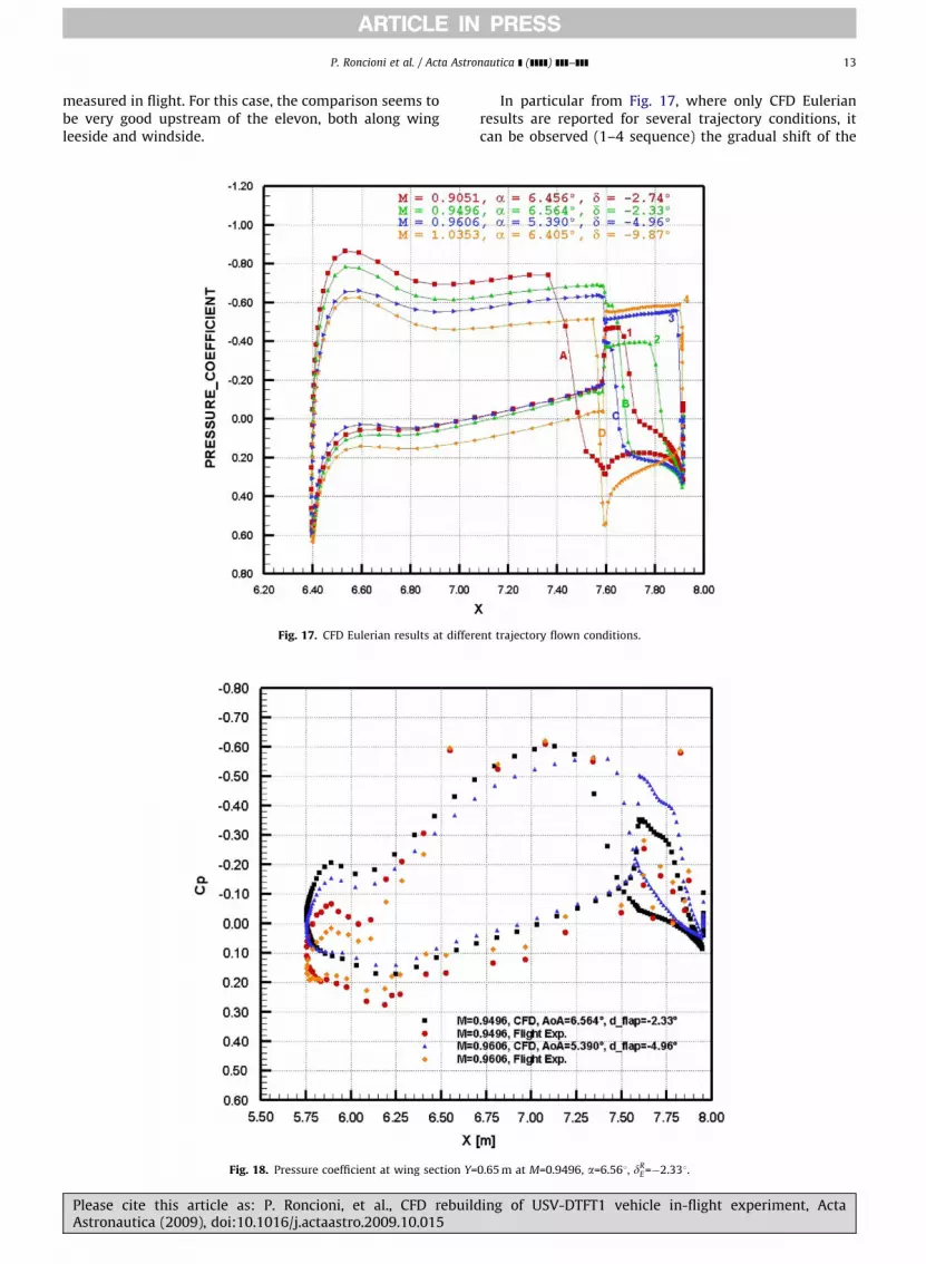
measured in flight. For this case, the comparison seems tobe very good upstream of the elevon, both along wingleeside and windside.

Fig. 17. CFD Eulerian results at differ

Fig. 18. Pressure coefficient at wing section Y=

Please cite this article as: P. Roncioni, et al., CFD rebuildAstronautica (2009), doi:10.1016/j.actaastro.2009.10.015

In particular from Fig. 17, where only CFD Eulerianresults are reported for several trajectory conditions, itcan be observed (1–4 sequence) the gradual shift of the

ent trajectory flown conditions.

0.65 m at M=0.9496, a=6.561, dRE=�2.331.

ing of USV-DTFT1 vehicle in-flight experiment, Acta

ARTICLE IN PRESS

P. Roncioni et al. / Acta Astronautica ] (]]]]) ]]]–]]]14

windside recompression shock (just downstream theexpansion wave) towards the flap trailing edge.Moreover, in the figure the A–D sequence shows theinitial leeside shock shift (from M=0.9051 to 0.9496), andthe subsequent assessment towards the flap hinge linewith a little upstream shift.

The compression peak (Cp=0.6) remains almost con-stant with an increasing Mach number, while theexpansion peak is gradually decreased (this is due to thepresence of strong three-dimensional effects along thewing span). Note as the angle of attack is nearly equal forthe four reported cases except for the case M=0.9606, thatis characterized by an incidence of about one degreelower.

The comparison at the wing section Y=0.65 m (seeFig. 18), located on the wing strake, shows, around thewing leading edge, a shift between the CFD viscouspredicted and in-flight measured pressure coefficients,

Fig. 19. Pressure coefficient at wing leading edge mea

Fig. 20. Time history of some leeside p

Please cite this article as: P. Roncioni, et al., CFD rebuildAstronautica (2009), doi:10.1016/j.actaastro.2009.10.015

at both M=0.9496 and 0.9606, and a quite good similartrend in the remaining part of wing section.

It is interesting to note as the case at M=0.9606 shows,both numerically and experimentally, an interceptedarea coherent with the lower angle of attack (upstreamthe flap zone) and the higher flap deflection angle(over the flap zone).

The analysis of Fig. 19, where the pressure coefficientdistributions along a section aligned with the wingleading edge are reported, at M=0.9496, shows a goodagreement between CFD results and in-flightmeasurements on the windside leading edge area. Onthe contrary, a disagreement is observed on the wingleeside towards both the tip and the root of the wing.

In particular, the analysis of wing tip region indicates thatduring the flight a large separation has occurred (as a result ofa wing tip-vortex detachment), while for the wing rootprobably there has been a malfunctioning of some leeside

surement line. M=0.9496, a=6.5641, dRE =�2.331.

ressure taps near to the fuselage.

ing of USV-DTFT1 vehicle in-flight experiment, Acta

ARTICLE IN PRESS

P. Roncioni et al. / Acta Astronautica ] (]]]]) ]]]–]]] 15

pressure taps, as also confirmed by the time evolution ofpressure measurements 1–4 of Fig. 19, shown in Fig. 20,where the sudden change of working of pressure tap 1 (theclosest to the fuselage) can be clearly appreciated.

Fig. 21. Pressure coefficient at nose sections X=0.85

Fig. 22. Pressure coefficient along vertical tail measu

Please cite this article as: P. Roncioni, et al., CFD rebuildAstronautica (2009), doi:10.1016/j.actaastro.2009.10.015

From Fig. 21 a very good comparison between CFDpredictions and in-flight measurements can be observedfor the nose section at X=0.99 m, whilst a less goodagreement can be seen for section at X=0.85 m. This is

and X=0.99 m. M=0.9496, a=6.5641, dRE =�2.331.

rement line. M=0.9496, a=6.5641, dER=�2.331.

ing of USV-DTFT1 vehicle in-flight experiment, Acta

ARTICLE IN PRESS

P. Roncioni et al. / Acta Astronautica ] (]]]]) ]]]–]]]16

probably due to the air data boom mounted on the nosevehicle, whose aerodynamic interference with the vehiclehas not been accounted for in the CFD simulations.

Fig. 23. Vertical tail pressure coefficient contours and ski

Fig. 24. Pressure coefficient along v

Please cite this article as: P. Roncioni, et al., CFD rebuildAstronautica (2009), doi:10.1016/j.actaastro.2009.10.015

The CFD simulated pressure coefficient distribution atthese sections has been simply mirrored (computationshave been performed on half vehicle), and the general good

n friction lines distribution at M=0.9396, a=6.5641.

ertical tail measurement line.

ing of USV-DTFT1 vehicle in-flight experiment, Acta

ARTICLE IN PRESS

P. Roncioni et al. / Acta Astronautica ] (]]]]) ]]]–]]] 17

agreement can justify the hypothesis of assumingno sideslip (b=�0.701 in this flight condition) in thesimulations, and is a further verification of the measuredangle-of-attack. This means that the front fuselage pressuretaps could be possibly used as a flush air data system(FADS).

Note that some measurements on the fuselage upperpart are clearly outliers for both sections, and they mustbe discarded from the analysis.

The comparison between CFD predicted and in-flightmeasured pressure coefficient along the vertical tailmeasurement line, at M=0.9496, is reported in Fig. 22.The comparison between viscous turbulent simulationand flight measurements shows a good agreement for thecompression peak at the leading edge, and for a large partof the vertical tail. A small but not negligible side forcegenerated by this control device (of course cancelled bythe presence of the symmetric tail), and a small effect ofthe rudder deflection (dR

R ¼ �0:553 in this flight condition)can be also remarked.

It is important to note the great difference betweenEulerian and Navier–Stokes simulation, being this latter

Fig. 25. Comparison between temporal history of flight measured global coeffic

bullets). (For interpretation of the references to the color in this figure legend,

Please cite this article as: P. Roncioni, et al., CFD rebuildAstronautica (2009), doi:10.1016/j.actaastro.2009.10.015

clearly able to capture the recompression or shock waveinside the channel between the two vertical tails (its naturedepends upon the position of the measurement line on thevertical tail, see also Fig. 23).

From the Eulerian simulations reported in Fig. 24, it can,however, be observed the gradual shift of the shock wavetowards the tail trailing edge.

5.5. Comparison between CFD results and flight experiment:

aerodynamic coefficients

Some comparisons between in-flight measured aero-dynamic coefficients, pre-flight ADB predictions and CFDpost-flight rebuilding are shown versus mission time inthe following Fig. 25.

The solid and dashed blue lines represent, respectively,the nominal flight measured data together with themeasurements error; the solid pink line corresponds tothe ADB model evaluated along the flown trajectory,while the dashed pink lines represent the pre-flightestimated ADB uncertainties. Finally, the two viscous

ient (blue line), ADB pre-flight prediction (pink line) and CFD data (gray

the reader is referred to the web version of this article.)

ing of USV-DTFT1 vehicle in-flight experiment, Acta

ARTICLE IN PRESS

P. Roncioni et al. / Acta Astronautica ] (]]]]) ]]]–]]]18

turbulent CFD simulations at M=0.9496 and M=0.9606 areindicated with gray bullets. Regarding the lift coefficientCL (diagram on the top) it can be observed that differencesexist between the flight measurements and ADB predic-tions, especially in the first part of the trajectory. Beingtypically the lift coefficient the easiest force coefficient tobe predicted, it is probable that the majority of thedifference is due to the error in the angle of attackmeasurement. Moreover, the CFD data well compare bothwith flight measurements and ADB model prediction. Thediagram in the middle of Fig. 25 shows a very goodagreement between flight, ADB and post flight CFD for thedrag coefficient CD. The same can be said for the pitchingmoment coefficient represented in the diagram on thebottom of Fig. 25 in terms of centre of pressure percentageposition, Xcp. In flight trimmed condition the pitchingmoment is zero and the centre of pressure of the vehiclelies on the centre of mass (71% of body length for thepresent case); in fact, apart for the region at about 31 s inwhich the vehicle is suddenly pitched down, the flightmeasured Xcp (blue line) is almost constant at a value of71%. Therefore, the difference between the predicted Xcp

and the centre of mass (CoM) is an indication of thegoodness of pitching moment prediction. Regarding CFDdata, it can be noted the perfect agreement for the case atM=0.9606 while the point at M=0.9496 exhibits a residualnose-up moment. Again, this fact reflects the strongsensitivity of pressure distributions at this Mach number,as already demonstrated above.

6. Conclusions

Aim of this paper has been to show some CFDrebuilding results of the aerodynamic experiment per-formed during the first Dropped Transonic Flight Test ofthe Italian USV FTB-1 vehicle, mission flown on lastFebruary 24th, 2007 from the base of Arbatax in Sardinia,Italy. The main target of this post-flight activity has beento compare CFD results with the database of in-flightmeasurements of global (forces, moments) and local(static pressures) aerodynamic parameters, this in orderto support and improve the CFD tools employed for thevehicle’s design.

As an overall goal of the USV project, this in-flightexperimentation relies on the evaluation of the wholepredictive capabilities and in its improvement finalized todesign risk reduction.

Some selected flight conditions have been numericallyrebuilt by means of numerical simulations (both Eulerianand Navier–Stokes), the attention being focused to thesurface pressure distributions to be correlated with in-flight pressure measurements. The comparison betweenCFD results and in-flight pressure measurements hasshown that a good agreement has been achieved on thewing, especially on the levels of pressure coefficient alongthe leeside and the windside, including the expansion andthe compression peaks downstream of the wing leadingedge stagnation point. It is also evident as Euleriancomputations do not predict the deterioration of pressurefield on leeside due to the large separated area existing at

Please cite this article as: P. Roncioni, et al., CFD rebuildAstronautica (2009), doi:10.1016/j.actaastro.2009.10.015

relatively high angles of attack. In particular, at M=0.9496(fully transonic regime) the viscous turbulent simulationshave properly predicted the strong and highly non-linearshock wave/boundary layer interaction phenomenon, alsoassessing a strong sensitivity to a 0.01 variation of flightMach number, with the consequent separation on thewing leeside.

The good agreement between predictions and mea-surements on the front fuselage section justifies thehypothesis of assuming no sideslip in the simulations,and is a further verification of the measured angle-of-attack despite the fact that in the first section of the frontfuselage a not very good agreement has been detected dueto the aerodynamic interference of the air boom. More-over, the comparison is also good along the measurementline on the vertical tail.

Regarding global aerodynamic coefficients, it must behighlighted that the agreement between the results ofAerodynamic Prediction Model, the flight recorded dataand the numerically rebuilt flight condition is rather goodboth for lift and drag coefficients.

The present CFD simulations have been finalised atreproducing the most relevant fluid dynamic phenomenacharacterizing the USV FTB-1 aerodynamics, the finalobjective being to compare numerical results to flight dataand to improve and/or assess the entire CFD methodology.A first step of this process has been afforded in the presentpost-flight analysis and will be continued within the otherscheduled flight missions.

Further analyses will be dedicated to a deeperinvestigation of the sensitivity of CFD results with respectto the flight condition’s uncertainty, turbulence andtransition modelling, etc.

Acknowledgements

The authors are grateful to the staff of the CIRA USVProgram, mainly to Mr. Giuseppe Guidotti, Dr. Piero DeMatteis and the Program Manager Dr. Gennaro Russo.Moreover, a special thank goes to all the engineers andtechnicians who contributed to the experimental set-up,and to Dr. Giuliano Ranuzzi for his precious supportduring the CFD activity.

References

[1] M. Pastena, et al. PRORA USV1: The first Italian experimentalvehicle to the aerospaceplane, in: 13th AIAA/CIRA InternationalSpace Planes and Hypersonic Systems and Technologies Confer-ence, Capua, Italy 16-20/05/05, AIAA-2005-3406.

[2] G. Russo, PRORA-USV: closer space and aeronautics, in: KeynoteLecture at the West-East High Speed Flow Field (WEHSFF-2007)Conference, 19–22 November 2007, Moscow, Russia.

[3] G.C. Rufolo, M. Marini, P. Roncioni, S. Borrelli, In Flight AerodynamicExperiment for the Unmanned Space Vehicle FTB-1, First CEASEuropean Air and Space Conference, Berlin, Germany, September10–13, 2007.

[4] G.C. Rufolo, P. Roncioni, M. Marini, S. Borrelli, Post flightaerodynamic analysis of the experimental vehicle PRO.R.A. USV1,AIAA-2008-2661, in: 15th AIAA/AHI International Space Planes andHypersonic Systems and Technologies Conference, Dayton, OH,USA, 28 April–1 May, 2008.

[5] G. Ranuzzi, S. Borreca, CLAE Project. H3NS: Code DevelopmentVerification and Validation, CIRA-CF-06-1017, 2006.

ing of USV-DTFT1 vehicle in-flight experiment, Acta

ARTICLE IN PRESS

P. Roncioni et al. / Acta Astronautica ] (]]]]) ]]]–]]] 19

[6] H.K. Myong, N. Kasagi, A new approach to the improvement of thek–e turbulence model for wall-bounded shear flows, JSME Interna-tional Journal Series II 33 (1) (1990) 63–72.

[7] G.C. Rufolo, P. Roncioni, M. Marini, R. Votta, S. Palazzo, Experi-mental and numerical aerodynamic data integration and aero-database development for the PRORA-USV-FTB_1 reusable vehicle,AIAA paper 2006-8031, in: 14th AIAA/AHI International SpacePlanes and Hypersonic Systems and Technologies Conference,Canberra, Australia, November 6–9, 2006.

[8] G.J. Brauckmann, X-34 vehicle aerodynamic characteristics, Journalof Spacecraft and Rockets 36 (2) (1999).

[9] B.N. Pamadi, G.J. Brauchmann, Aerodynamic characterization anddevelopment of the aerodynamic database of the X-34 RLV, in:International Symposium on Atmospheric Reentry Vehicles andSystems, Paper no. 17.1, Arcachon, France, March 16–18, 1999.

[10] C.G. Miller, Development of X-33/X-34 AerothermodynamicData Bases: Lessons Learned and Future Enhancements, October1999.

[11] S. Palazzo, M. Manco, CIRA USV programme, transonic wind tunneltest results on the USV FTB-1 scaled model in longitudinal andlateral-directional flight, CIRA-CF-04-0435, 2005.

Please cite this article as: P. Roncioni, et al., CFD rebuildAstronautica (2009), doi:10.1016/j.actaastro.2009.10.015

[12] A.D. Gardner, M. Jacobs, Force and moment measurements on ‘PRORA-USV 1:30 FTB1 model’ in DNW-TWG June–July 2005 experimentdocumentation and results, DNW IB 224-2005-C-11, August 2005.

[13] A.D. Gardner, M. Jacobs, Force and moment measurements on‘PRORA-USV 1:30 FTB1 model’ in DNW-TWG January 2006experiment documentation and results, DNW IB 224-2006-C-24,January 2006.

[14] B.R. Cobleigh, Development of the X-33 aerodynamic uncertaintymodel, NASA TP-1998-206544, April 1998.

[15] P.J. Roache, Verification and Validation in Computational Scienceand Engineering, Hermosa Publishers, New Mexico, 1998.

[16] P. Roncioni, G.C. Rufolo, R. Votta, M. Marini, An extrapolation-to-flight methodology for wind tunnel measurements applied to thePRORA-USV FTB1 vehicle, IAC-06-D2.3.09, in: 57th InternationalAstronautical Congress, Valencia, Spain, October 2–6, 2006.

[17] Assessment of experimental uncertainty with application to windTUNNEL testing, S-071A-1999, American Institute of Aeronauticsand Astronautics.

[18] Guide for the verification and validation of computational fluiddynamics simulations, G 077-1998, American Institute of Aero-nautics and Astronautics, January 14, 1998.

ing of USV-DTFT1 vehicle in-flight experiment, Acta