Canard Cycles in Global Dynamics

arX

iv:0

912.

2885

v1 [

mat

h.D

S] 1

5 D

ec 2

009

CANARD CYCLES IN GLOBAL DYNAMICS

ALEXANDRE VIDAL AND JEAN–PIERRE FRANCOISE

Submitted for publication on November 15, 2009.

Abstract. Fast-slow systems are studied usually by “geometrical dissec-tion” [4]. The fast dynamics exhibit attractors which may bifurcate underthe influence of the slow dynamics which is seen as a parameter of the fastdynamics. A generic solution comes close to a connected component of thestable invariant sets of the fast dynamics. As the slow dynamics evolves, thisattractor may lose its stability and the solution eventually reaches quicklyanother connected component of attractors of the fast dynamics and the pro-cess may repeat. This scenario explains quite well relaxation oscillations andmore complicated oscillations like bursting. More recently, in relation bothwith theory of dynamical systems [11] and with applications to physiology[10, 26], a new interest has emerged in canard cycles. These orbits share theproperty that they remain for a while close to an unstable invariant set (eithersingular set or periodic orbits of the fast dynamics). Although canards werefirst discovered when the transition points are folds, in this article, we focuson the case where one or several transition points or “jumps” are insteadtranscritical. We present several new surprising effects like the “amplifica-tion of canards” or the “exceptionally fast recovery” on both (1+1)-systemsand (2+1)-systems associated with tritrophic food chain dynamics. Finally,we also mention their possible relevance to the notion of resilience which hasbeen coined out in ecology [19, 22, 23].

Introduction

Systems are often complex because their evolution involves different timescales. Purpose of this article is to present several phenomena which can beobserved numerically and analyzed mathematically via bifurcation theory.

A first approximation for the time evolution of fast-slow dynamics is often seenas follows. A generic orbit quickly reaches the vicinity of an attractive invariantset of the fast dynamics. It evolves then slowly close to this attractive partuntil, under the influence of the slow dynamics, this attractive part bifurcatesinto a repulsive one. Then, the generic orbit quickly reaches the vicinity ofanother attractive invariant set until it also loses its stability. This approachis a quite meaningful approximation because it explains many phenomena likehysteresis cycles, relaxation oscillations, bursting oscillations [13, 27, 28] and

1991 Mathematics Subject Classification. Primary 34C29, 34C25,58F22.Key words and phrases. Fast-Slow Systems, Canards, Delay to Bifurcation, Transcritical

Bifurcation, Relaxation Oscillations.This research is supported by the Agence Nationale de la Recherche with the project ANAR.

1

http://arxiv.org/abs/0912.2885v1

2 ALEXANDRE VIDAL AND JEAN–PIERRE FRANCOISE

more complicated alternation of pulsatile and surge patterns of coupled GnRHneurons [6, 7].

Discovered by E. Benoit, J.-L. Callot, M. and F. Diener (see [3]), canardswere first observed in the van der Pol system:

(0.1)εx = y − f(x) = y − (x3

3+ x2)

y = x − c(ε)

where c(ε) ranges between some bounds:

(0.2) c0 + exp(

− α

ε2

)

< c(ε) < c0 +

(

− β

ε2

)

A canard is an orbit which remains for a while in a small neighborhood ofa repulsive branch of the critical manifold y = f(x) i.e. a connected set ofrepulsive points for the fast dynamics. In the following, we consider the canardphenomenon in its broader sense of delay to the bifurcation of the underlyingfast dynamics under the influence of the slow dynamics. More recently, F.Dumortier and R. Roussarie [11] contributed to the analysis of such orbits byblowing-up techniques and introduced the notion of canard cycle. There are nowseveral evidences showing the relevance of this notion to explain experimentalfacts observed in physiology (see [10, 26]).

The systems presented here display anomalous long delay to ejection fromthe repulsive part of the fast dynamics.

1. Enhanced delay and canard cycles of planar (1+1)–dynamics

1.1. Dynamical Transcritical Bifurcation.

The classical transcritical bifurcation occurs when the parameter λ in theequation:

(1.1) x = −λx + x2

crosses λ = 0. Equation (1.1) displays two equilibria, x = 0 and x = λ. Forλ > 0, x = 0 is stable and x = λ is unstable. After the bifurcation, λ < 0, x = 0is stable and x = λ is unstable. The two axis have “exchanged” their stability.

The terminology “Dynamical Bifurcation” (due to R. Thom) refers to the sit-uation where the bifurcation parameter is replaced by a slowly varying variable.In the case of the transcritical bifurcation, this yields:

(1.2)x = −yx + x2

y = −ε

where ε is assumed to be small. This yields:

x = −(−εt + y0)x + x2, (y0 = y(0))

which is an integrable equation of Bernoulli type. Its solution is:

x(t) =x0 exp[−Y (t)]

1 − x0

∫ t0exp[−Y (u)]du

, (x0 = x(0))

CANARD CYCLES IN GLOBAL DYNAMICS 3

where:

Y (t) =∫ t

0

y(s)ds =∫ t

0

(−εs + y0)ds = −εt2

2+ y0t

Figure 1. Orbits of system (1.2) starting from (0.05i, 1), fori = 1, .., 6, with ε = 0.1. The critical set – formed by the singularpoints of the fast dynamics – is shown in green and red. On thisset, the red points are repulsive for the fast dynamics and thegreen points are attractive. Each orbit reaches a neighborhoodof the attractive manifold x = 0, y > 0, goes down along x = 0.When y becomes negative, despite the repulsiveness of x = 0, y <0, each orbit remains for a very long time close to x = 0 beforedrifting away.

If we fix an initial data (x0, y0), y0 > 0, 0 < x0 < y0/2, and we consider thesolution starting from this initial data, we find easily that it takes time t = y0/εto reach the axis y = 0. If x0 is quite small, that means the orbit stays closerand closer of the attractive part of the critical manifold until it reaches the axisx = y and then coordinate x starts increasing. But now consider time cy0/ε,1 ≤ c ≤ 2. Then, a straightforward computation shows that:

Y (t) = c(

1 − c

2

)

y20

ε=

k

ε

and:

x(t) = O

x0e−

k

ε

1 − 2x0

y0


This shows that, despite the repulsiveness of the half-line x = 0, y < 0 for thefast dynamics, the orbit of (1.2) remains for a very long time close to x = 0,indeed x(cy0/ε) < 2x0 for ε small enough (see Figure 1). Note that, afterwardsfor larger time, the orbit blows away from this repulsive axis. This phenomenon,although quite simply explained, is of the same nature as the delay to bifurcationdiscovered for the dynamical Hopf bifurcation, see for instance [1, 5, 12, 29]. Thiswell-known effect is instrumental in the systems we study in this article. Somerelated work has been done in computing entry-exit relation for the passagenear single turning points (see [2, 9]).

1.2. Enhanced delay to bifurcation.

Consider the system:

(1.3)x = (1 − x2)(x − y)y = εx

The critical set – defined as the set of singular points of the fast dynamics –is the union of the straight lines x = −1, x = 1, and y = x. In the following,we call “slow manifolds” the two straight lines x = −1 and x = 1, as they areinvariant for the critical system (1 − x2)(x − y) = 0, y = x. A quick analysisshows that, as the slow variable y (considered as a parameter) evolves, the fastsystem undergoes two transcritical bifurcations: at x = −1 for y = −1, at x = 1for y = 1.

As we recalled in Subsection 1.1, a typical orbit starting from an initial data(x0, y0), |x0| < 1, close to (x = −1, y > −1), first goes down along x = −1 anddisplays a “delay” along the repulsive part of the slow manifold (x = −1, y <−1). Then, under the influence of the fast dynamics, it quickly reaches theattractive part (x = 1, y < 1) and moves upward to the other transcriticalbifurcation point. There, it again displays a delay along the repulsive part (x =1, y > 1). Then, it quickly reaches (x = 1, y > −1) and starts again. Hence,there is a mechanism of successive enhancements of the delay to bifurcationafter each oscillation generated by the hysteresis. We proved in [14] the:

Theorem 1. For all initial data inside the strip −1 < x < 1, for all δ and for

all T , the corresponding orbit spends a time larger than T within a distance less

than δ to the repulsive part of the slow manifolds.

We also proved in [14] the:

Theorem 2. Given any initial data (x0, y0) outside the strip |x| ≤ 1, the cor-

responding orbit is asymptotic to y = x.

1.3. Structural stability of the enhanced delay.

The theory of the structural stability of fast-slow systems remains to be found.In this subsection, we actually adopt a very pragmatic approach and restrict


Figure 2. Typical orbits of (1.3) with ε = 0.1 starting from apoint near the origin in panel 1) and from various initial datasoutside the strip |x| < 1 in panel 2). Double arrows are added onthe fast parts of the orbits and single arrows on the slow parts.Panel 1): The delay to the transcritical bifurcation undergone bythe orbit is enhanced at each passage. Consequently, the timetaken to escape a given neighborhood of x = −1, y < −1 on onehand and a given neighborhood of x = 1, y > 1 on the other handis longer for each oscillation than for the preceding one, althoughthese half-lines are repulsive for the fast dynamics.Panel 2): Each orbit is asymptotic to y = x.These numerical simulations were performed with order 4 Runge-Kutta integration scheme (absolute error value: 10−9 ; relativeerror value: 10−12 ; mean integration step: 10−5).

ourselves to numerical simulations. We perturb the system by adding an ar-bitrary small perturbation generated by a chaotic system, more precisely theRossler system [25].

(1.4)εx = (1 − x2)(x − y) + αn(t)y = x

where n(t) is the first variable of a Rossler system:

(1.5)n = −u − vu = n + auv = b + (n − c)v

with a = 0.1, b = 0.1, and c = 14 with some fixed initial data.We choose α quite small. The perturbation does not change the behavior of

the typical orbit for a while. It starts to oscillate between x = 1 and x = −1: itremains for a long time alternatively near each of these lines and undergoes fast


motions after ejection. But, as the orbit approaches closely these axes (withinthe distance of α), the small chaotic perturbation becomes operating and movesslightly the orbit outside of the strip. After crossing one of the straight linesx = −1 or x = 1, the orbit moves quickly to the axis y = x as previously shown.

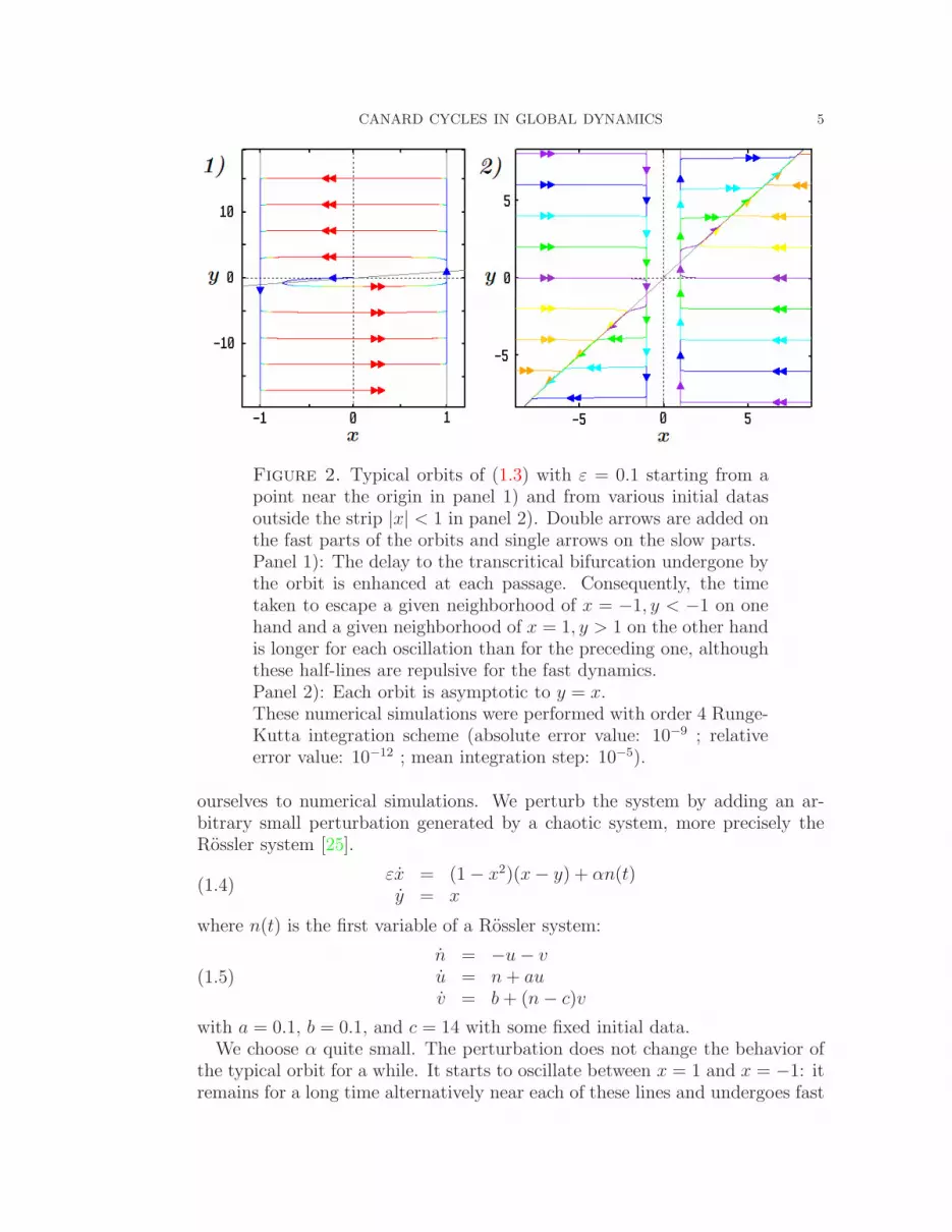
Figure 3. Example of an orbit of (1.4), with ε = 0.5 startingfrom (x, y) = (10−3, 0) for α = 10−4. Double arrows are added onthe fast parts of the orbit and single arrows on the slow parts.

Figure 3 displays an example of such an orbit starting from (0.001, 0) forα = 10−4. Despite the very small magnitude of the perturbation – less than3.10−3 – the orbit exits the strip |x| ≤ 1 before the third oscillation around theorigin. This simulation shows the loss of the oscillatory behavior as, under theinfluence of a perturbation of very small magnitude, the orbit crosses one ofthe slow manifolds as soon as x is sufficiently close to −1 or 1. We have thusobtained numerical evidence that the system is not structurally stable.

It is interesting to point out the fact that the numerical simulation of (1.3)highlights also this structural unstability. In fact, the integration scheme itself– whatever the integration step and the tolerances – provides errors. They giverise in the long run to intrinsic approximation: after many oscillations, the orbitstarting from |x| < 1 passes so close to the slow manifolds that the numericalintegration leads, sooner or later, to the approximation x = 1 or x = −1 or caneventually cross one of these lines.

1.4. Canard cycle for a double transcritical system.

In this subsection, we introduce a new system inspired by the preceding (1.3):

(1.6)x = (1 − x2)(x − y)y = εx(y + b)(a − y)

where a, b > 1 are parameters. The critical set is the same as the critical setof (1.3), formed by the three straight lines of equation x = −1, x = 1 and


y = x. The dynamics displays again two transcritical bifurcations: at x = −1for y = −1, at x = 1 for y = 1. But, the novelty is in the factors (a − y) and(y + b) in y which yield bounded orbits. We restrict the phase space to thecompact set:

K = (x, y)| − 1 ≤ x ≤ 1,−b ≤ y ≤ aAs for (1.3), the origin is a repulsive focus of (1.6). Except the origin, the

singular points of (1.6) in K are the summits of the rectangular boundary ofK, (−1,−b), (1,−b), (1, a), (−1, a), and are all of saddle type. As the straightlines x = −1, x = 1, y = a, y = −b are invariant under the flow of (1.6), wededuce the stable and unstable manifolds of each saddle:

saddle stable manifold unstable manifold(−1,−b) x = −1, y < a y = −b, x < 1(1,−b) y = −b, x > −1 x = 1, y < a(1, a) x = 1, y > −b y = a, x > −1(−1, a) y = a, x < 1 x = 1, y > −b

Consequently, the interior of K is invariant under the flow and contains onlya repulsive focus. The boundary of K is a graphic (ω-limit set formed by theunion of the saddles with their separatrices).

Following the study on the dynamical transcritical bifurcation, one expectsthat the value of y along an orbit oscillates between −b and min(a, b+2) if a ≥ bor between −min(b, a + 2) and a if a < b. However, the exponential attractionof x = −1, −1 < y < a (resp. x = 1, −b < y < 1), formed by attractive pointsof the fast dynamics, produces a delay to bifurcation and keeps the orbit nearx = −1, −b < y < −1 (resp. x = 1, 1 < y < a), formed by repulsive points ofthe fast dynamics. The delay could be great enough so that the orbit reachesa small neighborhood of y = 0. Hence, after the fast motion, the orbit tracksthe other manifold x = 1, −b < y < 1 (resp. x = −1, −1 < y < a) even closerthan during the preceding passage. The delay obtained afterwards is then againenhanced, as the orbit approaches even closer the slow manifolds. Hence, anorbit starting near the origin, after several oscillations, reaches alternatively asmall neighborhood of both y = a and y = −b, whatever the values of a and b.

Figure 4 illustrates this global behavior with fine step numerical simulationsfor various sets of parameter values. As expected, the smaller ε, the faster theorbit reaches a given neighborhood of x = −1 (resp. x = 1). Starting near theorigin, if ε is small (for instance, equal to 0.5 for the simulations presented inFigure 4), a few oscillations suffice to obtain a part close to the graphic.

Thus, the orbits of system (1.6) generate a new type of canards. On thecontrary of the canards discovered in the solutions of the van der Pol system, allthe orbits of system (1.6) starting from K\(0, 0) display delays to bifurcation.Moreover, we have a very simple way to modulate these delays by choosing the


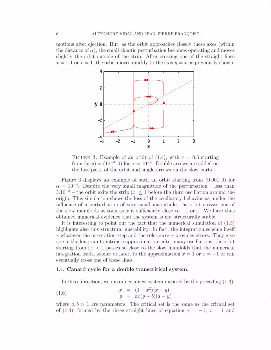
Figure 4. Orbits (red) of (1.6) for ε = 0.5, b = 2 and respec-tively a = 5 in panel 1) and a = 30 in panel 2). In both cases,the initial data is (10−3, 0). Comparison of panels 1) and 2) showsthat, whatever the values of a and b, the orbit enters alternativelysmall neighborhood of x = −1, x = 1, y = −b and y = a (bluestraight lines). These numerical simulations were performed withorder 4 Runge-Kutta integration scheme (absolute error value:10−9 ; relative error value: 10−12 ; mean integration step: 10−6).

parameter values a and b. It is worth noticing that, as in system (1.3), smallperturbations may provoke dramatic changes in the orbits.

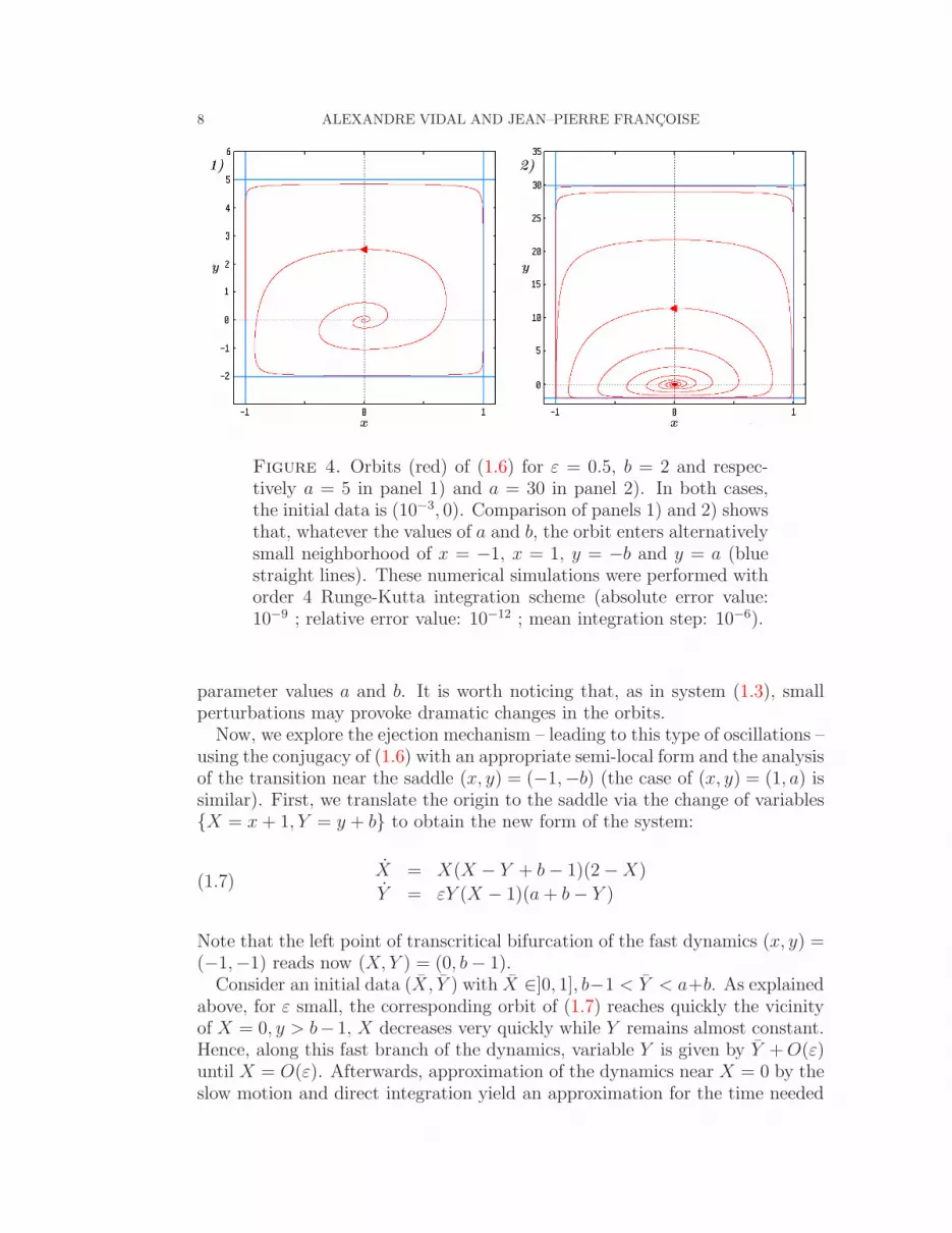
Now, we explore the ejection mechanism – leading to this type of oscillations –using the conjugacy of (1.6) with an appropriate semi-local form and the analysisof the transition near the saddle (x, y) = (−1,−b) (the case of (x, y) = (1, a) issimilar). First, we translate the origin to the saddle via the change of variablesX = x + 1, Y = y + b to obtain the new form of the system:

(1.7)X = X(X − Y + b − 1)(2 − X)

Y = εY (X − 1)(a + b − Y )

Note that the left point of transcritical bifurcation of the fast dynamics (x, y) =(−1,−1) reads now (X, Y ) = (0, b − 1).

Consider an initial data (X, Y ) with X ∈]0, 1], b−1 < Y < a+b. As explainedabove, for ε small, the corresponding orbit of (1.7) reaches quickly the vicinityof X = 0, y > b− 1, X decreases very quickly while Y remains almost constant.Hence, along this fast branch of the dynamics, variable Y is given by Y + O(ε)until X = O(ε). Afterwards, approximation of the dynamics near X = 0 by theslow motion and direct integration yield an approximation for the time needed


to reach Y = b − 1:

TY →b−1 =ε→0

1

ε(a + b)ln

[

(a + 1)Y

(b − 1)(a + b − Y )

]

+ O(1)

The leading term of the x-component C exp(−k/ε) displays:

C = (b − 1)2b−1a+b (a + 1)2

a+1a+b(1.8)

k =2

a + b

[

(b − 1) ln(Y ) + (a + 1) ln(a + b − Y )]

> 0(1.9)

We now study the delay to bifurcation and consider the entry of the orbitscoming from above Y = b− 1. Hence, we consider initial values of X which areexponentially small with respect to ε: C exp(−k/ε).

To specify the transition induced by the flow near the saddle, we consider thetwo sections:

Σin = (X, δ)|0 < X ≤ η(1.10)

Σout = (η, Y )|0 < Y ≤ δ(1.11)

with η > 0 a small fixed parameter and 0 < δ ≤ b − 1. We note:

U = (X, Y )|0 < X ≤ η, 0 < Y ≤ δthe rectangle delimited by Σin, Σout and the stable and unstable manifolds ofthe saddle (see Figure 5).

Figure 5. The transition function induced by the flow of (1.7)is well-defined from Σin into Σout.

Hence, as Y < 0 in (X, Y )|0 < X < 1, 0 < Y < X + b − 1 and δ ≤ b − 1,any orbit starting from Σin enters U and escapes from U through Σout. Thus,the transition function induced by the flow is well-defined from Σin into Σout.


As X is small in U (smaller than η), system (1.7) is conjugated to:

(1.12)X = 2(b − 1)X − 2XY

Y = εY

Note that (X, Y ) = (0, b − 1) is also a point of transcritical bifurcation for thissystem. Direct integration provides the orbit from (X0, δ):

X(t) = X0 exp

[

2(b − 1)t +2δ

ε

(

e−εt − 1)

]

Y (t) = δe−εt

As explained previously, we consider initial data of type X0 = C exp(−k/ε),where k, C > 0. If η < C, for ε small enough, i.e.:

ε < − k

ln ηC

(X0, δ) lies in Σin. If η ≥ C, as ε, k > 0, all values of ε fulfill this property.The time T needed to go from (X0, δ) to (η, Y (T )) ∈ Σout along the flow is

the solution of:

2(b − 1)T +2δ

εe−εT =

k

ε+ ln

η

C+

2δ

ε

The solution T can be expressed via the “Lambert function” WL – inversefunction of w → wew (see [8]). This yields:

(1.13) T =1

εWL

(

− δ

b − 1exp

(

−ǫ ln(η/C) + k + 2δ

2(b − 1)

))

+1

2(b − 1)

(

lnη

C+

k + 2δ

ε

)

As expected, the transition time is O(1/ε) and the leading term of T is:

(1.14) T =ε→0

1

ε

[

WL

(

− δ

b − 1e−

2δ+k

2(b−1)

)

+2δ + k

2(b − 1)

]

+ O(1)

This displays the transition function (X0, δ) → (η, Yout(X0)) with:

(1.15) Yout(Ce−k

ε ) =

δ exp

[

−WL

(

− δ

b − 1exp

(

−ǫ ln(η/C) + k + 2δ

2(b − 1)

))

+1

b − 1

(

lnη

C+

k + 2δ

ε

)]


This shows that, even if the transition time tends to +∞, the exit functiondisplays as O(1)-leading term:

(1.16) Yout(Ce−k

ε ) =ε→0

Y 0

out(Ce−k

ε ) + O(ε)

=ε→0

δ exp

[

−WL

(

− δ

b − 1e−

2δ+k

2(b−1)

)

− 2δ + k

2(b − 1)

]

+ O(ε)

Hence, the longer the orbit has remained near the slow manifold, the strongerthe ejection (to reach the neighborhood of (η, Y 0

out) given by (1.16)) is. Thisproperty of the orbits – staying a very long time near the repulsive part ofthe slow manifold without squashing on the y-nullcline – together with theincreasing strength of ejection is what we call the “exceptionally fast recovery”.Similar study can be done for the other transition of (1.6) and this leads tosimilar results (where a and b are exchanged).

Finally, note that, for given values of parameter a, b, ε, the values of param-eters k and C in (1.14) and (1.16) are approximated for the global dynamicsusing (1.8) and (1.9).

2. Saddle-node transcritical ejection in aprey-predator-superpredator model

2.1. Tritrophic food chain dynamics.

In the late seventies, interest in the mathematics of tritrophic food chain mod-els (composed of prey, predator and superpredator) appear (see, for instance,[15, 16]). Related predator-prey models with parasitic infections were studiedlater [17]. In the nineties, in [18, 24] and [20], the existence of chaotic attractorswas discussed. There are many more recent contributions, that we can not referin more details (see, for instance, [21, 28]).

We investigate here the following:

dU

dT= U

(

R(

1 − U

K

)

− A1V

B1 + U

)

dV

dT= V

(

E1

A1U

B1 + U− D1 −

A2W

B2 + V

)

(2.1)

dW

dT= εW

(

E2

A2V

B2 + V− D2

)

which represents the interactions between three populations U , V and W . Thevariable U stands for the prey, V for its predator and W for a superpredatorof V . The threshold constant K > 0 and the intrinsic growth rate of the preyR > 0 characterize the logistic evolution of U .


The predator–prey interactions are described by two Holling type II factorsdefined by the positive parameters:

Aj : the maximum predation rates

Bj : the half-saturation constants

Dj : the death rates

Ej : the efficiencies of predation

j = 1 relates to the predator V , j = 2 relates to the superpredator W . Itis assumed that the evolution of the superpredator is slower than those of thepredator and the prey. Then we introduce different time scales by means of theconstant 0 < ε ≪ 1.

2.2. Bifurcations of the fast dynamics.

The global behavior of this system (existence of global periodic orbit, bifurca-tions of limit cycles, early crisis in the predator membership) has been studiedin [27] and [28]. We recall briefly the classical situation of interest for us forwhich the system is bistable.

In order to obtain a simpler and more useful analytic form, Klebanoff andHastings proposed in [20] the following rescalings:

(2.2) x =U

K, y =

V

KE1

, z =W

KE1E2

, t = RT

which yields:

x = x(

1 − x − a1y

1 + b1x

)

= f(x, y, z)

y = y

(

a1x

1 + b1x− d1 −

a2z

1 + b2y

)

= g(x, y, z)(2.3)

z = εz

(

a2y

1 + b2y− d2

)

= h(x, y, z)

where aj, bj , dj, j = 1, 2 are positive parameters (see [20] or [27] for their expres-sions in function of Aj , Bj, Dj, Ej , R and K. All axes and faces of the positiveoctant R

3+ are invariant sets of (2.3). Thus, we limit the phase space to this

positive octant.Considering the slow variable z as a parameter, we describe the sequence of

bifurcations undergone by the two-dimensional fast dynamics. To this purpose,it is convenient to introduce the critical set:

(2.4) C = (x, y, z) ∈ R3

+|f(x, y, z) = 0, g(x, y, z) = 0formed by the singular points of the so-called Boundary-Layer System (BLS),obtained from (2.3) with ε = 0. For any point (x, y, z) ∈ C, (x, y) is a singularpoint of the fast dynamics for z = z. In the following, we note π the projectionfrom R

3+ into R

2+: π(x, y, z) = (x, y).


First, we assume:

(2.5) G = a1 − d1(1 + b1) > 0

to ensure that the singular point:

(2.6)

(

d1

G + d1

,G

(G + d1)2, 0

)

lays in the phase space R3+.

The critical set writes C = ∆ ∪ L where:

∆ = (1, 0, z)|z ∈ R+(2.7)

L =

(x, yL(x), zL(x)) ∈ R3

+|x ∈ [0, 1]

(2.8)

and:

yL(x) =1

a1

(1 − x) (1 + b1x)(2.9)

zL(x) =(a1x − d1 (1 + b1x)) (a1 + b2(1 − x)(1 + b1x))

a1a2(1 + b1x)(2.10)

Note that ∆ always intersects L at the point T = (1, 0, zT ) where:

(2.11) zT =G

a2(1 + b1)> 0

In the following, we assume that d1 is small enough so that:

(2.12) there is a point xP > 0 so that z′L(xP ) = 0.

We note P = (xP , yP , zP ) = (xP , yL(xP ), zL(xP )). Let us remark that, underassumption (2.12), zT < zP . Consequently, L is ∩-shaped in R

3+ (cf. Figure 6)

and we note:

• for each z ∈ ]zT , zP [, Sz the unique point (x, yL(x), z) ∈ Lsuch that x > xP ; LS = ∪

zT <z<zP

Sz ;

• for each z ∈ [0, zP [, Rz the unique point (x, yL(x), z) ∈ Lsuch that x < xP ; L± = ∪

0<z<zP

Rz.Thus, L = T ∪ LS ∪ P ∪ L± (see Figure 6).

The points π(Sz) are saddle type singular points of the fast dynamics, (1, 0) isa saddle for z < zT and an attractive node for z > zT . Additionally, we assumethat d1 is small enough such that there exists a point zH ∈]zT , zP [ so that:

for 0 ≤ z < zH , π(Rz) is a repulsive focus,

for zH ≤ z < zP , π(Rz) is an attractive focus.

Figure 6 displays C and its splitting according to the nature of the singularpoints for the fast dynamics. It can be seen as a bifurcation diagram of thefast dynamics as the bifurcation parameter z varies. Hence, as z decreases, thefollowing sequence of bifurcations occurs:

• for z > zP , the attractive node (1, 0) is the unique singular point.


Figure 6. Critical set of (2.3) (in red) – set of singular pointsof the Boundary-Layer System (BLS) obtained by setting ε = 0.It is splitted according to the nature of the singular points forthe fast dynamics with the corresponding value of z: ∆− andL− formed by attractive nodes, ∆S and LS by saddles, L+ byrepulsive foci. The points P , H , T are respectively the points ofsaddle-node, Hopf and saddle-node transcritical bifurcation of thefast dynamics. For z ∈ [0, zH [, the repulsive focus π(Rz) ∈ L+ issurrounded by an attractive limit cycle of the fast dynamics. Theunion M of these limit cycles (in green) is an invariant attractivemanifold for the (BLS).

• as z = zP , an inverse saddle-node bifurcation occurs at (xP , yP ).• for zH < z < zP , there are three singular points: the attractive node

(1, 0), the saddle π(Sz), the attractive focus π(Rz).• as z = zH , π(Rz) undergoes a supercritical Hopf bifurcation.• for zT < z < zH , there are three singular points: the attractive node

(1, 0), the saddle π(Sz), the repulsive focus π(Rz) surrounded by anattractive limit cycle, born from the Hopf bifurcation.

• as z = zT , a saddle-node transcritical bifurcation occurs at (1, 0) (π(Sz)and (0, 1) exchange their stability).

• for 0 ≤ z < zT , there are two singular points in the positive octant: thesaddle (0, 1) and the repulsive focus surrounded by an attractive limitcycle.


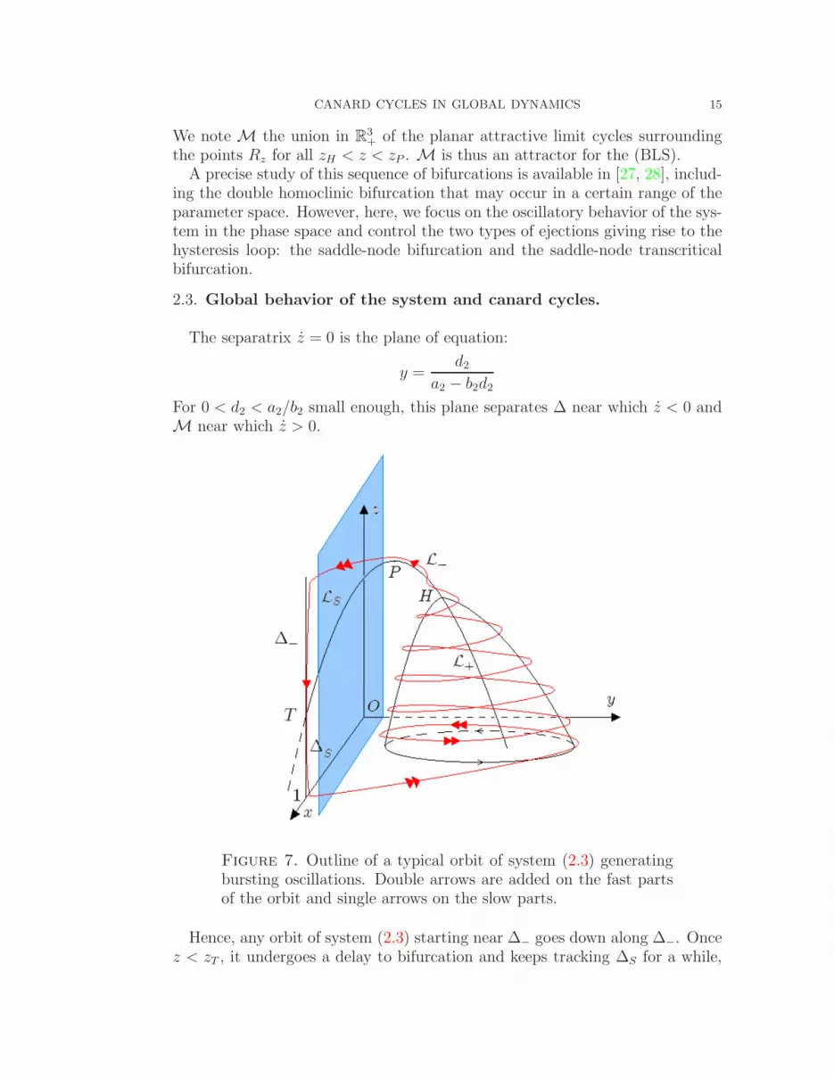
We note M the union in R3+ of the planar attractive limit cycles surrounding

the points Rz for all zH < z < zP . M is thus an attractor for the (BLS).A precise study of this sequence of bifurcations is available in [27, 28], includ-

ing the double homoclinic bifurcation that may occur in a certain range of theparameter space. However, here, we focus on the oscillatory behavior of the sys-tem in the phase space and control the two types of ejections giving rise to thehysteresis loop: the saddle-node bifurcation and the saddle-node transcriticalbifurcation.

2.3. Global behavior of the system and canard cycles.

The separatrix z = 0 is the plane of equation:

y =d2

a2 − b2d2

For 0 < d2 < a2/b2 small enough, this plane separates ∆ near which z < 0 andM near which z > 0.

Figure 7. Outline of a typical orbit of system (2.3) generatingbursting oscillations. Double arrows are added on the fast partsof the orbit and single arrows on the slow parts.

Hence, any orbit of system (2.3) starting near ∆− goes down along ∆−. Oncez < zT , it undergoes a delay to bifurcation and keeps tracking ∆S for a while,


although this branch is formed by saddles of the fast dynamics. After thisdelay, the orbit quickly reaches the vicinity of M. It goes up while spiralingaround M, then around L−. As z becomes larger than zP , the orbit reachesthe vicinity of ∆− and repeats the same sequence of motions. Figure 7 displaysthe geometric invariants of the fast dynamics and a schematic orbit of (2.3). Inthis setting, the delay to the transcritical bifurcation, that the orbit undergoes,qualifies the terminology of canard cycle.

Figure 8 displays a numerical simulation of a typical orbit of (2.3) with:

a1 = 0.8, b1 = 4, d1 = 0.1, ε = 0.1,a2 = 42, b2 = 40, d2 = 1.

Figure 8. Orbit of system (2.3) with the parameter values givenin the table of Subsection 2.3. Double arrows are added on thefast parts of the orbit and single arrows on the slow parts.

2.4. Local form near the saddle.

The most surprising behavior of these orbits is the long time needed to escapea neighbordhood of the point (1, 0, 0) and the “exceptionally fast recovery” of thevariable y. In this subsection, we perform successively two changes of variablesto obtain an appropriate local form near the saddle.

The Jacobian matrix associated with the system (2.1) at the singular point(x, y, z) = (1, 0, 0) reads:

−1 − a1

1+b10

0 a1

1+b1− d1 0

0 0 −εd2


It admits −1, a1

1+b1− d1 = G

1+b1and −εd2 as eigenvalues. Under the assumption

(2.5), the singular point (1, 0, 0) is then a saddle with a two-dimensional stablemanifold and a one-dimensional unstable manifold.

Eigenvectors associated with the eigenvalues are:

eigenvalue eigenvector−1 (1, 0, 0)G

1+b1(−1, 1

a1(G + 1 + b1), 0)

−εd2 (0, 0, 1)

Set:

α =1

a1

(G + 1 + b1) = 1 − (1 + b1)(d1 − 1)

a1

The parameter α is positive under the assumption (2.5) (G > 0).Hence, via the change of variables:

x = 1 − X − Y

y = αY

z = Z

the singular point (x, y, z) = (1, 0, 0) translates to (X, Y, Z) = (0, 0, 0). Now,the eigendirections of the saddle coincide with the (X, Y, Z)-axis. In this newsystem of coordinates, (2.3) reads:

X = −(1 − X − Y )(X + Y )

+Y

[

−1 +(X − Y )(d1 − 1)

1 + b1(1 + X − Y )− a2Z

1 + b2αY

]

Y = Y

[

a1(1 + X − Y )

1 + b1(1 + X − Y )− d1 −

a2Z

1 + b2αY

]

(2.13)

Z = Zε[

a2αY

1 + b2αY− d2

]

This allows to consider X > 0 in the following.Actually, an eigenvector associated with each saddle (0, 1) of the fast dynamics

writes:

(2.14) (β(Z), 1) =

(

a2Z(1 + b1)

1 + b1 + G − a2Z(1 + b1), 1

)

This vector is well-defined in the positive octant as long as:

Z <1 + b1 + G

a2(1 + b1)=

1

a2

(

1 +G

1 + b1

)

Thus, under the assumption (2.5), it is well-defined at least for Z ∈ [0, zT ]and β(Z) > 0. Note that, for Z = zT , this vector gives the central directionassociated with the 0 eigenvalues of the non hyperbolic point (0, 0) of the fastdynamics.


For each Z ∈ [0, zT ], the vector (2.14) gives the tangent line to the unstablemanifold of the saddle (0, 0) of the fast dynamics with Z = Z. Thus, we havean approximation for X and Y small of the invariant manifold of (2.13) withε = 0. As this manifold is normally attractive, it persists for ε > 0 small enoughinto a normally attractive manifold of (2.13). We proceed with another changeof variables:

u = X − β(Z)Y

y = Y

z = Z

locally near X = Y = 0, 0 ≤ Z ≤ zT , system (2.13) reads:

u = −u + O(εv, uv, u2)

v = G′v − a2vw + vO(u, v)(2.15)

w = −εd2w + wO(v2)

where:

G′ =G

1 + b1

=a1

1 + b1

− d1

The perturbed attractive manifold in this new set of parameters is approximatedby u = 0, 0 ≤ Z ≤ zT .

The flow on the invariant perturbed manifold is conjugated – locally nearu = v = 0 – to the system:

v = v(

a1

1 + b1

− d1

)

− a2vw(2.16)

w = −εd2w

After setting w = 2Y/a2 and replacing εd2 by ε, we recognize the normal form(1.12) introduced in Subsection 1.4 with parameter values G′ = (b − 1) > 0.

2.5. Transition function: recovery of the predator.

Consider the two sections:

Σin = (u, v, δ)|0 < v ≤ η(2.17)

Σout = (u, η, Y )|0 < u ≤ ξ, 0 < w ≤ δ(2.18)

where η, ξ > 0 are small but fixed parameters and 0 < δ < zT (see (2.11)) isfixed. We note:

U = (u, v, w)|0 < u ≤ ξ, 0 < v ≤ η, 0 < w ≤ δThe preceding analysis shows that, for ε small enough, an orbit of (2.16) startingfrom Σin enters U and exits from U . Hence, the transition function induced bythe flow of (2.16) is well-defined from Σin into Σout.


As the typical orbits of system (2.3) enter an exponentially small neighbor-hood of ∆S (see Figures 7, 8 and Subsection 2.3), we restrict initial data of(2.16) to be exponentially close to X = Y = 0 in Σin. Thus, consider:

u0 = C1e−

k1ε(2.19)

v0 = C2e−

k1ε(2.20)

By direct application of the local analysis made in Subsection 1.4, we obtainthe leading term of the transition time from (u0, v0, δ) ∈ Σin to Σout along theflow of (2.16):

T =ε→0

1

εd2

[

WL

(

−a2δ

G′e−

a2δ+k2d2G

)

+a2δ + k2d2

G′

]

+ O(1)

The transition function (u0, v0, δ) → (uout(u0, v0), η, wout(u0, v0)) can be speci-fied as well:

(2.21) uout(C1e−

k1ε , C2e

−k1ε )

∼ε→0

C1e−

k1ε

[

−WL

(

−a2δ

G′e−

a2δ+k2d2G′

)

− a2δ + k2d2

d2G′

]

(2.22) wout(C1e−

k1ε , C2e

−k1ε )

=ε→0

δ exp

[

−WL

(

−a2δ

G′e−

a2δ+k2d2G′

)

− a2δ + k2d2

d2G′

]

+ O(ε)

It is worth noticing that the u-component of the transition function tendsactually to 0 as ε → 0, but that the w-component experiments a basal threshold,even if this threshold is very low.

2.6. Interpretation in terms of ecological parameters: loss of resilience.

In contrast with system (1.6), the two ejection mechanisms in (2.3) are pro-vided by different types of bifurcation of the fast dynamics: a saddle-node tran-scritical bifurcation at T and a saddle-node bifurcation at P . Near P , canardscould eventually appear for which the orbit tracks the manifold LS formed bysaddle of the fast dynamics. However, this type of canards can occur only if P isnear the plane z = 0 (within a O(

√ε) distance). But the assumption that this

plane separates properly ∆ and the manifold M (d2 small enough) generallyforbids such behavior.

Hence, any orbit in the strictly positive octant displays, sooner or later, themotion described in Subsection 2.3 as there exists a globally attractive periodicorbit of this type (see [27, 28]). Thus, the entry of this periodic orbit – as theentry of any orbit after spiraling around M – in a given neighborhood of ∆occurs for z = zP + O(ε2/3). The delay to bifurcation after the passage in thevicinity of T is then mostly characterized by zP − zT . In fact, as calculated


for (1.6) in (1.9), the contraction exponent between ∆ and the orbit is chieflydetermined by zP − zT .

The “exceptionally fast recovery” that we have pointed out therein may havesome connection with the notion of “loss of resilience” which has been discussedin several dynamical models related to Ecology [19, 22, 23]. The long returntimes associated with a loss of resilience are caused by slow dynamics near theunstable equilibrium. We expect that new developments of this subject couldpossibly benefit of the notion of canards and canard cycles.

Acknowledgements: The numerical simulations were performed using XPP-AUT: http://www.math.pitt.edu/~bard/xpp/xpp.html

References

[1] Baer, S. M., Erneux, T. & Rinzel, J. [1989] “The slow passage through a Hopf bifurcation:Delay memory effects and resonance,” SIAM J. Applied Mathematics 49, 55–71.

[2] Benoit, E. [1981] “Equations differentielles: relation entree-sortie,” C. R. Academie desSciences de Paris 293, serie I, 293–296.

[3] Benoit, E., Callot, J.-L., Diener, F. & Diener, M. [1981] “Chasse au canard,” CollectaneaMathematica 31, 37–119.

[4] Borisyuk, A. & Rinzel, J. [2004] “Understanding neuronal dynamics by geometrical dis-section of minimal models,” in Methods and Models in Neurophysics, Les Houches Sum-mer School 1980 (Chow, C., Gutkin, B., Hansel, D. & C. Meunier), Elsevier New York,pp. 19–72.

[5] Candelpergher, B., Diener, F. & Diener, M. [1990] “Retard a la bifurcation : du local auglobal,” in Bifurcations of Planar Vector Fields, Proceedings of the Luminy conference(Francoise, J.-P. & Roussarie, R.), Lecture Notes in Mathematics, vol. 1455, SpringerBerlin, pp. 1–19.

[6] Clement, F. & Francoise, J.-P. [2007] “Mathematical modeling of the GnRH-pulse andsurge generator,” SIAM J. Applied Dynamical Systems 6, 441–456.

[7] Clement, F. & Vidal, A. [2009] “Foliation-based parameter tuning in a model of theGnRH pulse and surge generator,” to appear in SIAM J. Applied Dynamical Systems.

[8] Corless, R. M., Gonnet, G. H., Hare, D. E. G., Jeffrey, D. J. & Knuth, D. E. [1996] “Onthe LambertW function,” Adv. Computational Mathematics 5, 329–359.

[9] De Maesschalk, P. & Dumortier, F. [2005] “Time analysis and entry-exit relation nearplanar turning points,” J. Differential Equations 215, 225–267.

[10] Desroches, M., Krauskopf, B. & Osinga, H. M. [2008] “Mixed-mode oscillations and slowmanifolds in the self-coupled FitzHugh-Nagumo system,” Chaos 18 (1).

[11] Dumortier, F. & Roussarie, R. [1996] “Canard cycles and center manifolds,” Mem. Amer-ican Mathematical Society 121, 1–100.

[12] Erneux, T., Reiss, E. L., Holden, L. J. & Georgiou, M. [1991] “Slow passage throughbifurcation and limit points. Asymptotic theory and applications,” in Dynamic Bifurca-

tions, Proceedings of the Luminy conference (Benoit, E.), Lecture Notes in Mathematics,vol. 1493, Springer Berlin, pp. 14–28.

[13] Francoise, J.-P. [2005] Oscillations en Biologie : Analyse qualitative et modeles, Springer,Collection: Mathematiques et Applications, vol. 46.

[14] Francoise, J.-P., Piquet, C. & Vidal, A. [2008] “Enhanced Delay to Bifurcation,” Bull.Belgian Mathematical Society – Simon Stevin 15, 825–831.

[15] Freedman, H. & Waltman, P. [1977] “Mathematical analysis of some three-species food-chain models,” Mathematical Biosciences 33, 257–276.

http://www.math.pitt.edu/~bard/xpp/xpp.html


[16] Gard, T. [1980] “Persistence in food chains with general interactions,” MathematicalBiosciences 51, 165–174.

[17] Hadeler, K. P. & Freedman, H. [1989] “Predator-prey populations with parasitic infec-tion,” J. Mathematical Biology 27, 609–631.

[18] Hastings, A. & Powell, T. [1991] “Chaos in a three-species food chain,” Ecology 72,896–903.

[19] Holling, C. S. [1973] “Resilience and stability of ecological systems,” Ann. Rev. Ecologyand Systematics 4, 1–23.

[20] Klebanoff, A. & Hastings, A. [1994] “Chaos in three species food chains,” J. MathematicalBiology 32, 427–451.

[21] Kooi, B. W., Boer, M. P. & Kooijman, S. A. [1998] “Consequences of population modelsfor the dynamics of food chains,” Mathematical Biosciences 153, 99–124.

[22] Ludwig, D., Walker, B. & Holling, C. S. [1997] “Sustainability, stability and resilience,”Conservation Ecology 1. http://www.consecol.org/vol1/iss1:art7/

[23] Martin, S. [2004] “The cost of restoration as a way of defining resilience: a viabilityapproach applied to a model of lake eutrophication,” Ecology and Society 9.http://www.ecologyandsociety.org/vol9/iss2/art8/

[24] Muratori, S. & Rinaldi, S. [1992] “Low- and high-frequency oscillations in three-dimensional food chain systems,” SIAM J. Applied Mathematics 52, 1688–1706.

[25] Rossler, O. E. [1976] “An equation for continuous chaos,” Physics Letters 57A, 397–398.[26] Toporikova, N., Tabak, J., Freeman, M. E. & Bertram, R. [2008] “A-type K+ current

can act as a trigger for bursting in the absence of a slow variable,” Neural Computation20, 436–451.

[27] Vidal, A. [2006] “Stable periodic orbits associated with bursting oscillations in populationdynamics,” Lecture Notes in Control and Information Sciences 341, 439–446.

[28] Vidal, A. [2007] “Periodic orbits of tritrophic slow-fast systems and double homoclinicbifurcations,” Discrete and Continuous Dynamical Systems – Series B suppl. vol., 1021–1030.

[29] Zoladek, H. [1990] “Remarks on the delay of the loss of stability of systems with chang-ing parameters,” in Bifurcations of Planar Vector Fields, Proceedings of the Luminyconference (Francoise, J.-P. & Roussarie, R.), Lecture Notes in Mathematics, vol. 1455,Springer Berlin, pp. 393–396.

Alexandre Vidal – Laboratoire Analyse et Probabilites,Universite d’Evry Val d’Essonne, Evry, [email protected]

Jean–Pierre Francoise – Laboratoire J.-L. Lions, UMR 7598, CNRS,Universite P.-M. Curie, Paris6, Paris, [email protected]

http://www.consecol.org/vol1/iss1:art7/

http://www.ecologyandsociety.org/vol9/iss2/art8/

mailto:[email protected]

mailto:[email protected]

Documents

Canard Cycles in Global Dynamics