Brownian Motion - Advanced Labs

Brownian Motion

Experiment BM

University of Florida — Department of PhysicsPHY4803L — Advanced Physics Laboratory

By Robert DeSerio & Stephen Hagen

Objective

A microscope is used to observe the motionof micron-sized spheres suspended in water.A digital video camera captures the motionwhich is then analyzed with a particle track-ing program to determine the path of indi-vidual spheres. The sphere’s random Brow-nian motion is analyzed with a spreadsheetto verify various theoretical predictions. Thedependence of the particle’s displacements ontime as well as various physical parameterssuch as the temperature, the suspension liq-uid’s viscosity and the sphere diameter isalso explored. Diffusion of dye-labeled DNAmolecules is also studied.

References

M.A. Catipovic, P.M. Tyler, J.G. Trapani, andAshley R. Carter, Improving the quantifica-tion of Brownian motion, Am. J. Phys. 81485-491 (2013).1

Daniel T. Gillespie, The mathematics ofBrownian motion and Johnson noise, Am. J.Phys. 64 225 (1996).2

D. Jia, J. Hamilton, L.M. Zaman, and A.Goonewardene, The time, size, viscosity, and

1http://dx.doi.org/10.1119/1.48035292http://dx.doi.org/10.1119/1.18210

temperature dependence of the Brownian mo-tion of polystyrene microspheres, Am J. Phys.75 111-115 (2007).3

P. Nakroshis, M. Amoroso, J. Legere, C.Smith, Measuring Boltzmanns constant usingvideo microscopy of Brownian motion, Am. J.Phys. 71 568-573 (2003).4

P. Nelson, Biological Physics: Energy, In-formation, Life, W. H. Freeman (2003).

P. Pearle et al., What Brown saw and youcan too, Am. J. Phys. 78 1278-1289 (2010).5

D.E. Smith, T.T. Perkins, S. Chu, Dy-namical scaling of DNA diffusion coefficients,Macromolecules 29 1372-1373 (1996).6

Brownian motion

Brownian motion refers to the continuous,random motion of microscopic particles thatare suspended in a fluid. Robert Brown in1827 described such motion in micron-sizedparticles that were released from the pollengrains of Clarkia pulchella, a flower that hadbeen discovered by Lewis and Clark a fewyears earlier. Although the biological origin ofthe particles at first suggested that this motionhad something to do with life, Brown quicklyrealized that all sorts of inorganic particles ex-

3http://dx.doi.org/10.1119/1.23861634http://dx.doi.org/10.1119/1.15426195http://dx.doi.org/10.1119/1.34756856http://pubs.acs.org/doi/abs/10.1021/ma951455p

BM 1

BM 2 Advanced Physics Laboratory

hibited the same motion. Granules of carbonsoot or ancient stone, when suspended in wa-ter, executed ceaseless motion with complex,apparently random trajectories. Although therate of motion depends on the size of the par-ticles and the temperature and viscosity of thefluid, the phenomenon is universal to particlesin a fluid.

Brown himself did not understand the phys-ical cause, but Einstein recognized that Brow-nian motion could be completely explained interms of the atomic nature of matter and thekinetic nature of heat: the fluid is composedof molecules that are in continuous motion atany finite temperature. A larger particle in thefluid is subject to frequent collisions that de-liver numerous small, random impulses, caus-ing the larger particle to drift gradually butirregularly through the fluid. In one of his fa-mous 1905 papers, Einstein showed that therate of Brownian motion is directly relatedto the microscopic Boltzmann constant kB,which sets the scale for the kinetic energy(∼ kBT ) carried by a water molecule at tem-perature T . kB is related to the macroscopicgas constant R = NAkBT by a factor of Avo-gadro’s number NA. As R is easily found ina benchtop experiment, the measurement ofkB reveals NA. Brownian motion is a directlink between two very different size scales inphysics: it originates in the microscopic mo-tion of atoms, molecules and the tiny scaleof their thermal energy, and it is observableas macroscopic motion that can be measuredat the bench of any reasonably well equippedlaboratory. Einstein’s work paved the wayfor Perrin’s measurements of Brownian mo-tion, which provided compelling support forthe atomic theory and earned the 1926 physicsNobel prize.

Kinetic theory

Before considering Brownian motion, weshould first recall certain aspects of the kinetictheory for the molecules of the fluid. Thesemolecules are in constant interaction with allother molecules, which together form a heatbath at temperature T . The equipartition the-orem of statistical physics requires that thekinetic energy in each spatial component ofthe molecular velocity has an ensemble aver-age value of kBT/2. For the x-direction thisimplies:

1

2m⟨v2x⟩

=1

2kBT (1)

Here m is the molecular mass and T is thetemperature. The angle brackets 〈〉 indicatean ensemble average, i.e. the average over alarge population of molecules. The ensembleaverage may be calculated if the probabilitydistribution for vx is known.

What is the probability distribution for thevelocity components? Each of the three spa-tial components of the molecular velocity isdistributed according to a Boltzmann distri-bution in the kinetic energy mv2/2 associatedwith that velocity component. This leads tothe so-called Maxwell Boltzmann distributionfor the probability that the molecule will havea velocity between vx and vx + dvx

dP (vx) =

√m

2πkBTe−mv

2x/2kBTdvx (2)

The square root prefactor is required for nor-malization ∫ ∞

−∞dP (vx) = 1 (3)

Equation 2 is a Gaussian probability distribu-tion with a mean of zero and a variance ofkBT/m. Of course, analogous expressions ap-ply to the y- and z-components of velocity.

December 28, 2015

Brownian Motion BM 3

The Maxwell-Boltzmann probability distri-bution for vx (Eq. 2) obeys the equipartitiontheorem because the average is⟨

v2x⟩

=

√m

2πkBT

∫ ∞−∞

v2xe−mv2x/2kBTdvx (4)

which leads to 〈v2x〉 = kBT/m, consistent withEq. 1.

For water molecules at room tempera-ture the average molecular speed is roughly600 m/s. Consequently there is plenty of mo-mentum in the fluid molecules that collidewith a small particle that is suspended in thefluid.

Consider a particle with mass M , suspendedin the fluid at r(t) and moving with velocityv(t). The particle is subject to a net force F(t)from the fluid. We can analyze the motionover a time interval dt that is sufficiently shortthat r(t) and v(t) can both be considered verynearly constant. For a Brownian particle, it isconvenient to analyze the motion by castingNewton’s second law in the form:

dr(t) = v(t)dt (5)

dv(t) =1

MF(t)dt (6)

F(t), which may depend on r and v, is eval-uated and the right sides of Eqs. 5 and 6 arecalculated. With the left sides defined by

dr(t) = r(t+ dt)− r(t) (7)

dv(t) = v(t+ dt)− v(t) (8)

the right-side values are then added to thevalues r(t) and v(t) to obtain updated valuesr(t+dt) and v(t+dt) at a time dt later. Start-ing from given initial conditions for r(0) = r0and v(0) = v0 at t = 0, the process is repeatedto obtain future values for r(t) and v(t) at dis-crete intervals.

The motion is said to be deterministic whenF(t) can be precisely determined from the val-

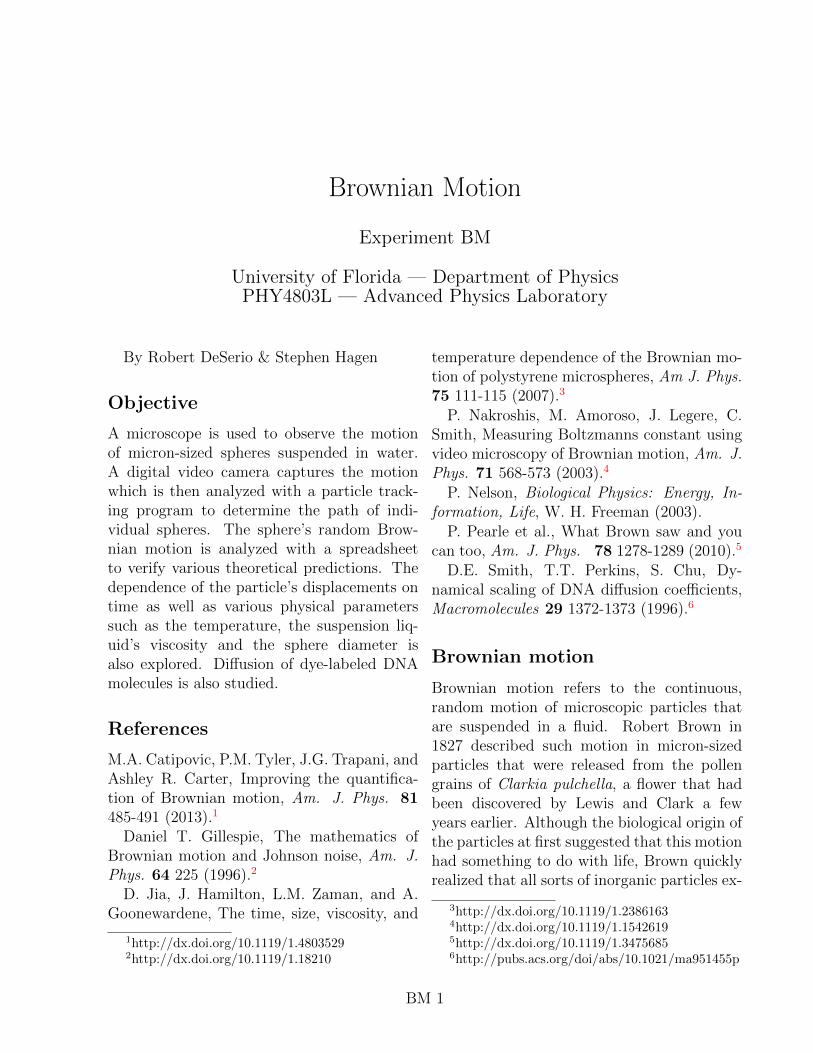
Figure 1: The molecules of the surrounding fluidundergo frequent collisions with a Brownian par-ticle (shown as large circle), delivering small ran-dom impulses Ji. There are many such impulsesin even a short interval dt.

ues of r(t), v(t), and t. For example, in a colli-sion between two particles with a known inter-action (such as the Coulomb or gravitationalforce) F(t) is deterministic and the motion isquite predictable.7

In Brownian motion, F(t) is created by thevery frequent collisions between the suspendedparticle and the molecules of the surroundingmedium, about 1019 collisions per second fora 1µm particle in water. Consider the forceFi(t) that acts on the Brownian particle dur-ing its collision with one individual moleculefrom the medium. That one collision deliversan impulse to the Brownian particle

Ji =

∫Fi(t)dt (9)

where the integral extends over the dura-

7Deterministic does not always mean predictable.Some perfectly precise forms of F(t) lead to chaoticsolutions that cannot be predicted far into the futureat all.

December 28, 2015


tion of the collision (Figure 1). The indi-vidual impulses Ji vary in magnitude and di-rection because the velocities of molecules inthe medium vary according to the Maxwell-Boltzmann distribution. Consequently the di-rection and magnitude of Fi(t) are highly vari-able. This variable impulse adds a randomcomponent to the net force on the particle.Both the force and the particle’s motion aresaid to be stochastic, and the motion of asingle particle is unpredictable. Rather thanfocusing on predicting individual trajectories,we aim to understand the motion in terms ofprobabilities and average behavior.

Dynamics of a Brownian particle

Because of the high collision frequency, we canchoose a time interval dt short enough thatr(t) and v(t) do not change significantly, yetlong enough to include thousands of collisions.Over such an interval, the value of F(t)dt inEq. 6 would properly be the sum of all im-pulses delivered during the interval dt

F(t)dt =∑i

Ji (10)

When the number of collisions during dtis large, we can use the central limit theo-rem to draw important conclusions about theform of F(t)dt even though we lack detailedknowledge of individual impulses. The centrallimit theorem states that if we add togethermany random numbers drawn from the sameprobability distribution, the sum will be aGaussian-distributed random number. This istrue regardless of the distribution from whichthe random numbers are drawn (e.g. Gaus-sian or not). More precisely, the theoremstates that if N individual random numbersxi are drawn from any probability distribu-tion that has mean µi and variance σ2

i , thenthe sum Σxi of those N numbers will itself be

a Gaussian-distributed random number withmean µ = Nµi and variance σ2 = Nσ2

i .Each cartesian component of Ji is a random

number from an (unknown) distribution andthus the central limit theorem applies to eachcomponent of Eq. 10. Remember, v(t) andr(t) do not change significantly over the in-terval dt; the probability distributions for thecomponents of Ji arise from the distribution ofvelocities for the colliding molecules and fromthe distribution of collision angles. Moreover,because the number of collisions N over a timeinterval dt will be proportional to dt, the cen-tral limit theorem implies that each compo-nent of F(t)dt will be a random number froma Gaussian distribution whose mean and vari-ance are both proportional to dt.

We do not expect that F(t) necessarily hasa mean value of zero. If the Brownian parti-cle has a net velocity v through the fluid, itwill collide with more molecules on its leadingside than on its trailing side, and so the forcewill be imbalanced. In fact we should expectthat F(t) will depend in part on the veloc-ity v(t) of the Brownian particle with respectto the bulk medium. Paul Langevin hypothe-sized that F(t)dt can be expressed

F(t)dt = −αv(t) dt+ F(r)(t) dt (11)

The term −αv describes a viscous drag forcethat is opposite in direction and proportionalto the particle’s velocity relative to the fluid.This had already been investigated by Stokes,who showed that the drag coefficient α for asphere of diameter d in a fluid of dynamic vis-cosity η is given by

α = 3πηd (12)

F(r)(t) is the random part of the collisionalforce. Langevin successfully characterized thispart and showed how it was responsible forBrownian motion.

December 28, 2015


We will use a shorthand notation

N(µ, σ2) (13)

to refer to a Gaussian distribution of mean µand variance σ2. For example,

vx = N

(0,kBT

m

)(14)

will be shorthand for the statement that thex-component of velocity for a molecule of massm is a random variable drawn from the Gaus-sian probability distribution of Eq. 2.

Any random number from a distributionwith a mean µ and variance σ2 can be consid-ered as the sum of the mean and a zero-meanrandom number having a variance σ2

N(µ, σ2) = µ+N(0, σ2) (15)

Then one may see how Eq. 11 is related toEq. 10 and the central limit theorem. Eachcartesian component of the −αv dt term inEq. 11 is the mean of the sum in the cen-tral limit theorem applied to that componentof Eq. 10. With the means accounted forby the −αv dt term, each component of theF(r)(t)dt term must be a zero-mean, Gaussian-distributed random number providing the ran-dom or distributed part of the central limittheorem.

Over time, the viscous drag force in Eq. 11will tend to eliminate any initial velocity of theparticle through the fluid; however the fluctu-ating force Fr(t) will prevent the particle fromever coming to rest. Regardless of the ini-tial velocity, random collisions with moleculesin the environment will deliver kinetic energyto the suspended particle and ensure that ithas mean kinetic energy as specified by theequipartition theorem and a velocity proba-bility distribution of the Maxwell Boltzmannform.

Exercise 1 Determine the room temperaturerms velocities (

√〈v2〉) of water molecules and

of 1µm diameter spheres in water. Assumethe spheres have the density of water.

Note that the F(r)(t) dt term (which drivesthe particle’s motion) and the viscous dragforce (which opposes it) will require a certainbalance if the velocity at equilibrium is to fol-low the Maxwell Boltzmann distribution. Thefluctuation-dissipation theorem describes thisbalance, relating the impulse delivered duringan interval dt to the viscous drag coefficientand the temperature as follows:

F (r)x (t)dt = N(0, 2αkBT dt) (16)

A similar equation holds for the y and z-components of F(r)(t). As α is the viscous dragcoefficient, Eq. 16 makes a fundamental con-nection between the fluid’s viscosity and tem-perature and the size of the fluctuating force.

Note that the mean, or −αv dt term, inEq. 11 is proportional to dt as required bythe central limit theorem. Note also that therandom F(r)(t)dt term also satisfies the the-orem in that its variance is proportional todt. These two proportionalities are required ifEqs. 5 and 6 are to give self-consistent solu-tions as the step size dt is varied.

Exercise 2 When solving differential equa-tions numerically (i.e., on a computer), thetime step dt must be chosen small enough thatr(t) and v(t) undergo only small changes dur-ing the interval. However, dt must not bemade too small because roundoff and other nu-merical errors occur with each step. Often,one looks at the numerical solutions for r(t)and v(t) as the step size dt is decreased, choos-ing a dt where there is little dependence on itssize.

Why do the mean and variance of F dt haveto be proportional to dt in order for the equa-tions of motion to be self consistent? Your

December 28, 2015


answer should take into account how the sumof two Gaussian random numbers behave (onaverage) and how v(t) (on average) wouldchange over one interval dt or over two in-tervals half as long.

We will take initial conditions at t = 0 ofr(0) = r0 and v(0) = v0. Thus, the particlebegins with a well defined position and veloc-ity. However, the nature of the stochastic forceimplies that the particle position and velocityfor t > 0 will be probability distributions thatchange with time. The references8 show howto integrate Eq. 11. Here we simply presentthe results without proof.

The solution for vx(t) can be written

vx(t) = N

(v0xe

−t/τ ,kBT

M(1− e−2t/τ )

)(17)

where

τ =M

α(18)

Analogous solutions are found for vy and vz.As required at t = 0, Eq. 17 has the valuevx(0) = N(v0x, 0) (i.e., the velocity is v0x).At t → ∞ it has the solution vx(∞) =N(0, kBT/M), i.e., the Maxwell-Boltzmanndistribution. Keep in mind that t→∞ reallymeans t� τ where, for a particle of size 1µmin water, τ ≈ 100 ns. Note how τ in Eq. 17describes the exponential decay of any initialvelocity and (within a factor of two) the ex-ponential approach to the equilibrium velocitydistribution: τ is such a short interval that theparticle’s velocity loses its initial value and be-comes Maxwell-Boltzmann-like very rapidly.

The probability distribution for the positionr(t) is slightly more complicated. With analo-gous solutions for y(t) and z(t), the result canbe expressed

x(t) = N(µx, σ2) (19)

8See especially D.T. Gillespie (1996).

where

µx(t) = x0 + vx0τ(1− e−t/τ ) (20)

and

σ2(t) =2kBT

α

[t− 2τ(1− e−t/τ ) (21)

+τ

2(1− e−2t/τ )

]For a particle released from rest at the origin

(r0 = 0, v0 = 0), the equilibrium positiondistribution then becomes

x(t) = N(0, σ2) (22)

Eq. 22 means that the probability for the par-ticle to have an x-displacement between x andx+ dx is given by

dP (x) =1√

2πσ2e−x

2/2σ2

dx (23)

where

σ2 =2kBTt

α= 2Dt (24)

Here we have defined the diffusion coefficientof the particle,

D =kBT

α(25)

The diffusion coefficient tells us how rapidlythe variance in the particle’s location growswith time.

The probability that the particle’s displace-ment will fall within a volume element dV =dx dy dz around a particular value of r is theproduct of three such distributions—one foreach direction x, y and z. Using r2 = x2 +y2 + z2, the product is

dP (r) =1

(2πσ2)3/2exp−r

2/2σ2

dV (26)

Consider a large number N of particlesplaced at the origin at t = 0. According to

December 28, 2015


Eq. 26, each will have the probability dP (r)to be in the volume element dV located atthat r. Consequently, the number of parti-cles in that volume element will be NdP (r)and their number density would be given byρ(r) = NdP (r)/dV or

ρ(r, t) =N

(2πσ2)3/2e−r

2/2σ2

(27)

where the (implicit) time dependence arisesbecause σ2 grows linearly in time via Eq. 24.The concentration profile of the particles is aGaussian function that becomes broader andflatter over time as the particles diffuse awayfrom the starting point.

The particles spread according to Eq. 27with Eq. 24 until hindered by the containerwalls. An observer might say that particles arebeing actively driven from regions of higherconcentration to regions of lower concentra-tion until they become uniformly distributedthroughout the suspension, although of coursethe motion of individual particles is random.

Fick’s second law of diffusion describes theflattening of ρ(r) over time.

dρ

dt= D∇2ρ (28)

Einstein realized how Fick’s second law is re-lated to Brownian diffusion and was the firstto relate D to σ.

Exercise 3 Show that ρ(r, t) satisfies Eq. 28with

σ2 = 2Dt (29)

Note that if a spherical particle (diameter d)moves in a fluid of viscosity η, we can combineEq. 24 with Eq. 12 and obtain

D =kBT

3πηd(30)

This is the famous Stokes-Einstein expressionfor the diffusion coefficient of a spherical par-ticle.

Exercise 4 Eq. 29 says the width of the parti-cle distribution increases with t. Qualitatively,this behavior is reasonable because with moretime for the random Brownian motion, onewould expect the values of r to become morespread out. Explain in a similar qualitativeway why the width of the distribution would beexpected to increase with T and decrease withη and d as predicted by Eq. 30.

Random walks and polymerchains

In this experiment you are going to study theBrownian motion of DNA molecules in wa-ter. The DNA strand coils up in a fairlyrandom fashion in water, and the rate of itsBrownian motion depends on the overall sizeof that random coil. Interestingly there is aclose analogy between a Brownian motion tra-jectory and the configuration of a disorderedchain molecule (polymer). Here we will exam-ine a simple model known as the freely jointedchain (FJC). The FJC model will allow us toestimate the probability distribution for thedistance between the two endpoints of a long,disordered polymer.

Imagine the polymer chain as consisting ofa very large number N of links, each of lengtha (Figure 2). Suppose that the links are freelyjointed so that the bond angle at the junctionof two successive links i and i + 1 can adoptany value, without bias. This may soundcompletely unrealistic, but for sufficiently longpolymers such as nucleic acids (DNA, RNA)and large unfolded protein molecules it can bea reasonable approximation. The bonds thatlink the monomers of a real chain do have someintrinsic stiffness, but if we define a “link” asa sufficiently long segment of that chain (i.e.containing several monomer units), then suc-cessive links really can adopt nearly any ori-entation with respect to each other.

December 28, 2015


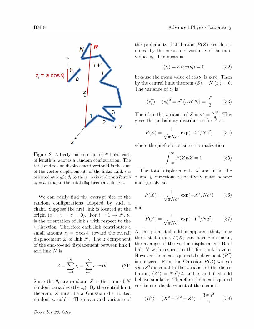
Figure 2: A freely jointed chain of N links, eachof length a, adopts a random configuration. Thetotal end to end displacement vector R is the sumof the vector displacements of the links. Link i isoriented at angle θi to the z−axis and contributeszi = a cos θi to the total displacement along z.

We can easily find the average size of therandom configurations adopted by such achain. Suppose the first link is located at theorigin (x = y = z = 0). For i = 1 → N , θiis the orientation of link i with respect to thez direction. Therefore each link contributes asmall amount zi = a cos θi toward the overalldisplacement Z of link N . The z componentof the end-to-end displacement between link 1and link N is

Z =N∑i=1

zi =N∑i=1

a cos θi (31)

Since the θi are random, Z is the sum of Nrandom variables (the zi). By the central limittheorem, Z must be a Gaussian distributedrandom variable. The mean and variance of

the probability distribution P (Z) are deter-mined by the mean and variance of the indi-vidual zi. The mean is

〈zi〉 = a 〈cos θi〉 = 0 (32)

because the mean value of cos θi is zero. Thenby the central limit theorem 〈Z〉 = N 〈zi〉 = 0.The variance of zi is⟨

z2i⟩− 〈zi〉2 = a2

⟨cos2 θi

⟩=a2

2(33)

Therefore the variance of Z is σ2 = Na2

2. This

gives the probability distribution for Z as

P (Z) =1√πNa2

exp(−Z2/Na2) (34)

where the prefactor ensures normalization∫ ∞−∞

P (Z)dZ = 1 (35)

The total displacements X and Y in thex and y directions respectively must behaveanalogously, so

P (X) =1√πNa2

exp(−X2/Na2) (36)

and

P (Y ) =1√πNa2

exp(−Y 2/Na2) (37)

At this point it should be apparent that, sincethe distributions P (X) etc. have zero mean,the average of the vector displacement R oflink N with respect to the first link is zero.However the mean squared displacement 〈R2〉is not zero. From the Gaussian P (Z) we cansee 〈Z2〉 is equal to the variance of the distri-bution, 〈Z2〉 = Na2/2, and X and Y shouldbehave similarly. Therefore the mean squaredend-to-end displacement of the chain is⟨

R2⟩

=⟨X2 + Y 2 + Z2

⟩=

3Na2

2(38)

December 28, 2015


Eq. 38 is remarkable in itself. It says that asthe length N of the polymer chain increases, itis not the mean displacement of the final linkthat grows in proportion to N . Rather it isthe mean squared displacement that grows inproportion to N . This is very similar to theBrownian particle trajectories above, wherethe mean squared distance traveled by the par-ticle grows in proportion to the duration t ofthe motion. Clearly the path taken by suc-cessive links of the chain is analogous to theirregular path taken by the Brownian parti-cle. An important difference is that the linksare all of the same length, whereas the “steps”taken by the Brownian particle are not. Stillthe result is essentially the same.

If you want to know what is the probabil-ity that the two ends of the chain are sepa-rated by a scalar distance R (i.e. irrespec-tive of orientation) then you need to find theprobability distribution for R as opposed toX, Y , Z. Start by multiplying the prod-uct P (X)P (Y )P (Z)dXdY dZ = P (R)dV tofind the probability that link N terminateswithin a particular volume element of sizedV = dXdY dZ located at R = (X, Y, Z)

P (R)dV =dV

(πNa2)3/2exp(−R2/Na2) (39)

In the exponent we have used the fact thatR2 = X2 + Y 2 + Z2. Then express dV inspherical polar coordinates (R, θ, φ) giving

P (R)dV =R2dR sin θdθdφ

(πNa2)3/2exp(−R2/Na2)

(40)If we are not interested in orientation then wecan integrate over the angles and focus on theprobability distribution for the magnitude R,

P (R)dR =

∫ 2π

φ=0

∫ π

θ=0

P (R)dV (41)

which gives

P (R)dR =4πR2dR

(πNa2)3/2exp(−R2/Na2) (42)

R ≥ 0 is the scalar distance from one end ofthe polymer chain to the other. While theaverage R is zero, the average R is clearlynonzero.

Exercise 5 Note the difference between P (R)of Eq. 39 and P (R) of Eq. 42. Sketch P (R)and P (R) vs. R. Explain why the functionsbehave so differently near R = 0. That is, whydoes P (R) have to be zero at R = 0 whereasP (R) does not?

Effective dimensions of a polymerchain

We understand how the length of a polymerchain relates to the overall dimension R of therandomly coiled molecule. How does R relateto the rate of its Brownian motion in a fluid?We have already seen the Stokes-Einstein re-lation Eq. 30 for diffusion of a spherical par-ticle. Given the diffusion rate of any otherparticle, we could characterize its motion bysaying that it diffuses with D = kBT/6πηRh

where Rh is an “effective” radius that dependson the size and shape of the particle. Thatis, Rh (known as the hydrodynamic radius) isthe radius of the sphere that would exhibit thesame diffusion coefficient. For biopolymers Rh

is difficult to calculate, but it is often well ap-proximated by a quantity known as the radiusof gyration, RG. RG describes9 the mass dis-tribution of the chain relative to the chain’scenter of mass. For the freely jointed chainyou can show that

R2G →

1

6

⟨R2⟩

=Na2

4(43)

9Specifically, R2G is the mean (over the whole chain)

of the squared distance from each link to the chain’scenter of mass.

December 28, 2015


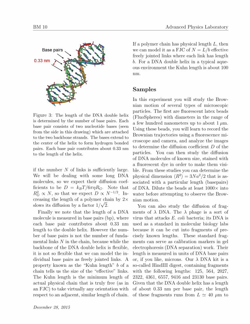
Figure 3: The length of the DNA double helixis determined by the number of base pairs. Eachbase pair consists of two nucleotide bases (seenfrom the side in this drawing) which are attachedto the two backbone strands. The bases extend tothe center of the helix to form hydrogen bondedpairs. Each base pair contributes about 0.33 nmto the length of the helix.

if the number N of links is sufficiently large.We will be dealing with some long DNAmolecules, so we expect their diffusion coef-ficients to be D = kBT/6πηRG. Note thatR2G ∝ N , so that we expect D ∝ N−1/2. In-

creasing the length of a polymer chain by 2×slows its diffusion by a factor 1/

√2.

Finally we note that the length of a DNAmolecule is measured in base pairs (bp), whereeach base pair contributes about 0.33 nmlength to the double helix. However the num-ber of base pairs is not the number of funda-mental links N in the chain, because while thebackbone of the DNA double helix is flexible,it is not so flexible that we can model the in-dividual base pairs as freely jointed links. Aproperty known as the “Kuhn length” b of achain tells us the size of the “effective” links.The Kuhn length is the minimum length ofactual physical chain that is truly free (as inan FJC) to take virtually any orientation withrespect to an adjacent, similar length of chain.

If a polymer chain has physical length L, thenwe can model it as a FJC of N = L/b effectivefreely jointed links where each link has lengthb. For a DNA double helix in a typical aque-ous environment the Kuhn length is about 100nm.

Samples

In this experiment you will study the Brow-nian motion of several types of microscopicparticles. The first are fluorescent latex beads(FluoSpheres) with diameters in the range ofa few hundred nanometers up to about 1 µm.Using these beads, you will learn to record theBrownian trajectories using a fluorescence mi-croscope and camera, and analyze the imagesto determine the diffusion coefficient D of theparticles. You can then study the diffusionof DNA molecules of known size, stained witha fluorescent dye in order to make them visi-ble. From these studies you can determine thephysical dimension 〈R2〉 = 3Na2/2 that is as-sociated with a particular length (basepairs)of DNA. Dilute the beads at least 1000× intowater before attempting to observe the Brow-nian motion.

You can also study the diffusion of frag-ments of λ DNA. The λ phage is a sort ofvirus that attacks E. coli bacteria; its DNA isused as a standard in molecular biology labsbecause it can be cut into fragments of pre-cisely known lengths. These standard frag-ments can serve as calibration markers in gelelectrophoresis (DNA separation) work. Theirlength is measured in units of DNA base pairsor, if you like, microns. Our λ DNA kit is aso-called HindIII digest, containing fragmentswith the following lengths: 125, 564, 2027,2322, 4361, 6557, 9416 and 23130 base pairs.Given that the DNA double helix has a lengthof about 0.33 nm per base pair, the lengthof these fragments runs from L ' 40 µm to

December 28, 2015


L ' 7.7 mm. Such long DNA strands adoptrandomly coiled configurations just like thefreely jointed chain discussed above. Conse-quently they diffuse at a rate D that shouldvary inversely as the RG of the strand, i.e.,inversely proportional to L1/2.

Exercise 6 From the known lengths of theHindIII fragments, the Kuhn length of theDNA double helix, and the Stokes Einstein re-lation, estimate the diffusion coefficients D ofthe different λ DNA fragment lengths.

Analyzing trajectories

The goal is to observe the trajectory of theBrownian particle and, from the particle’s dis-placement vs. time, determine the diffusion co-efficient D. Eq. 19 and Eq. 29 together statethat the particle’s mean squared displacementafter a time t is⟨

x2⟩

= σ2 = 2Dt (44)

(Remember that 〈x〉 = 0.) Therefore we canfind D from the slope of the average squareddisplacement vs. time: D = 〈x2〉 /2t. Youmight expect that a reasonable way to find Dis then to allow a particle (starting at x = 0)to move for a very long period t, and then di-vide its final squared displacement x2 by thetime period t. In fact this technique gives poorresults10, because the relation x2 ∝ t is onlytrue as an ensemble average: in practice youneed to measure a very large number of indi-vidual trajectories before their average 〈x2〉 /tgives D to satisfactory precision. This can bevery time consuming.

There are good alternatives however. Usinga microscope equipped with a scientific camerayou can collect a series of N image frames at

10Error and uncertainty in the analysis of Browniantrajectories is discussed in the article by M. Catipovicet al. (2013)

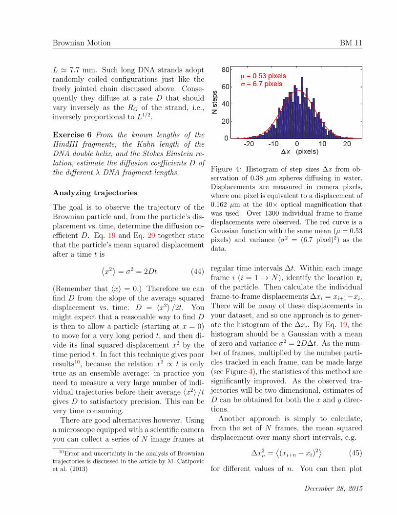
Figure 4: Histogram of step sizes ∆x from ob-servation of 0.38 µm spheres diffusing in water.Displacements are measured in camera pixels,where one pixel is equivalent to a displacement of0.162 µm at the 40× optical magnification thatwas used. Over 1300 individual frame-to-framedisplacements were observed. The red curve is aGaussian function with the same mean (µ = 0.53pixels) and variance (σ2 = (6.7 pixel)2) as thedata.

regular time intervals ∆t. Within each imageframe i (i = 1 → N), identify the location riof the particle. Then calculate the individualframe-to-frame displacements ∆xi = xi+1−xi.There will be many of these displacements inyour dataset, and so one approach is to gener-ate the histogram of the ∆xi. By Eq. 19, thehistogram should be a Gaussian with a meanof zero and variance σ2 = 2D∆t. As the num-ber of frames, multiplied by the number parti-cles tracked in each frame, can be made large(see Figure 4), the statistics of this method aresignificantly improved. As the observed tra-jectories will be two-dimensional, estimates ofD can be obtained for both the x and y direc-tions.

Another approach is simply to calculate,from the set of N frames, the mean squareddisplacement over many short intervals, e.g.

∆x2n =⟨(xi+n − xi)2

⟩(45)

for different values of n. You can then plot

December 28, 2015


∆x2n vs n, which should obey ∆x2n = 2n∆tD.

Of course, since the data contain fewer val-ues of (xi+n − xi)2 for larger values of n, theaveraging is less effective at large n and theproportionality ∆x2n ∝ n will be less well-determined at large n. In practice it may besufficient just to find the slope using the firsttwo points, n = 0, 1.

Hardware

The apparatus for this experiment is sim-ple. Although it is entirely possible to ob-serve Brownian motion in white light, the im-age analysis is a little easier (the particlesare easier to track) if they are observed influorescence instead of white light. Henceyou will use fluorescently dyed (stained) par-ticles. These absorb blue light and reemit itas green (fluorescent) light. Using the appro-priate color filters in the base of the micro-scope, the particles then appear in the im-ages as bright dots against a dark background.DNA is not naturally fluorescent in the visi-ble spectrum. Therefore, in order to make theDNA fluoresce, we add a small amount of dyeto the solution containing the DNA. The dye,SYTO 9, binds strongly to the DNA moleculesand causes them to fluoresce bright green un-der blue light illumination.

You will use an inverted fluorescence mi-croscope (Nikon Eclipse TS100-F model), tostudy the diffusing particles. The fluores-cence of the particles is excited by a mercuryarc lamp and the fluorescent emission passesthrough a filter set in the base of the micro-scope before going to either the eyepiece or thecamera.

The fluorescence of the particles will be onlydimly visible (if at all) to your eye. How-ever a sensitive camera will have no difficultyrecording the fluorescence. Therefore, for datacollection the fluorescent light will be sent di-

rectly to a camera. We use a cooled charge-coupled-device camera (“CCD camera”, An-dor Clara model) which provides an array of1360×1024 pixels in the focal plane of the mi-croscope. The pixels are square in shape, withdimensions 4.65× 4.65 µm. Particle displace-ments can be measured in camera pixels, atleast during data collection and preliminaryanalysis. Later you can convert from pixelunits to µm based on the magnification of themicroscope objective. The microscope pro-vides magnifications of 10×, 20×, or 40×. Youwill need to collect a series of image framesshowing the same group of particles, and thenanalyse these images (see below) to identifythe particle trajectories. You will probablyfind it convenient to collect the images at arate ∼ 0.5− 1 frame per second, using highermagnification for smaller particles only. Forexample, image at 40× for 0.38 µm diameterparticles.

Software

The PC attached to the microscope has soft-ware that controls the CCD camera, includingframe rate, exposure time, number of expo-sures, and other settings. You will need to ex-periment with it to learn how to obtain goodfluorescence images of the fluorescent beads.To adjust physical parameters such as themicroscope magnification and focus you willneed to physically adjust the microscope it-self. Note that you will need to determine thespatial calibration of the camera image (pixelsper micron), which will depend on the micro-scope magnification. The physical size of animage in the camera focal plane is simply re-lated to the size of the real object by a factor ofthe microscope magnification (i.e. the numberthat is inscribed on the microscope objective).You can calculate the size calibration of theimages by using the pixel size data above, and

December 28, 2015


then check it by imaging an object of knownsize such as a reticle.

The PC also has a popular software packageknown as ImageJ that will allow you to trackthe motion of particles between frames. Im-ageJ contains a particle detection and track-ing plugin (Mosaic) that will locate bright par-ticles against a dark background in your im-ages, find their coordinates in the image (inunits of pixels) and then track the same par-ticles from frame to frame, generating a list ofcoordinates (frame-to-frame) for each particlethat is tracked. This analysis includes someimportant parameters that determine how farthe particle is assumed capable of moving fromone frame to the next, as well as setting thethreshold for how clearly the particle shouldbe visible in the image before it is tracked.Once a particle moves more than a few µm inthe axial (z−direction) it will be out of focusand cannot be tracked accurately.

Finally you can import your trajectory datainto software such as Excel or Matlab in orderto further analyze the trajectory, as describedbelow.

Error sources

There are a few sources of error that you needto consider. First, it is very important thatthe fluid be stationary. If there is even a smallbulk motion of the fluid, such that the particledrifts with a net speed v in the x−direction,then the mean frame-to-frame displacementwill be v∆t. This drift will affect the variance,especially if the number of frames is small11.Be sure to allow your sample sufficient time af-ter preparation to equilibrate so that the drift

11Consider for example the case where N = 2 andonly two frames are studied. Then you cannot knowwhether to ascribe the particle’s motion during ∆t toBrownian motion or to drift. For larger N the situa-tion is less dire, but still requires caution.

velocity v = 0.

Through the Stokes Einstein formula thediameter d of the particles and the solventviscosity η are both potential sources of er-ror. However the manufacturer of the par-ticles (FluoSpheres, Molecular Probes) char-acterizes the diameter of the particles to lessthan 0.02 µm, so the size uncertainty con-tributes an error of no more than 2-5% forparticles in the size range of 0.5− 1 µm. Theviscosity of water is highly temperature sensi-tive, but you can measure room temperatureto an accuracy better than 1 ◦C and then lookup the viscosity at that temperature.

An important source of error arises in thedetermination of particle positions and frame-to-frame displacements. The ImageJ/Mosaicparticle-tracking algorithm offers parametersettings that adjust how well it recognizes thesame particle at different locations in adjacentimage frames. Although it is tempting to ad-just those settings so that the algorithm ag-gressively seeks and identifies lengthy (many-frame) trajectories of an individual particle,you do not need such long trajectories to per-form your data analysis. In fact they are likelyto introduce errors such as poor guesses ofthe location of out-of-focus particles, and mix-ups over which of the particles in one framewas seen at a similar location in the previ-ous frame. These errors lead e.g. to unphys-ically long ∆xi values. It is perfectly accept-able to employ more conservative settings thatoccasionally lose track of some particles, in ex-change for more accurate location data whenthose particles are seen.

Procedure

• First prepare a sample of spheres by di-luting the sphere suspension into deion-ized water. A large dilution of 1000× orgreater is appropriate.

December 28, 2015


• Use a pipette or syringe to load the sam-ple into the observation channel of theslide. We use the Ibidi type 81121 mi-crofluidic slide. This is a plastic slide con-taining a closed channel that is a few mil-limeters long and 0.1 mm deep. The slideis equipped with Luer fittings so that youcan load it with a standard syringe andthen cap the ends to prevent the fluidfrom evaporating. Be sure to fill the slideevenly so that the fluid comes to the sameheight in the Luer fittings at the two endsof the channel. Otherwise there will be apressure gradient in the channel and fluidwill tend to drift for some time, interfer-ing with your measurements.

• Allow the slide to equilibrate on the mi-croscope stage for 15-30 minutes beforeyou begin measurements in earnest.

• Use the multi-frame imaging function ofthe camera software to collect the tra-jectories of several Brownian particles atonce. You can set a frame rate (e.g. 2frames per second, ∆t = 0.5 s) on thecamera and collect a series of images.

• Load the images into the ImageJ andrun the particle tracking plugin, and thentransfer the results to Excel or Matlab.Generate the ∆x and ∆y displacementsand analyze as described above to obtainD for your particles.

• Based on the known size of the particles,the measured temperature in the room,and the tabulated dynamic viscosity η ofwater, you should be able to obtain anestimate for Boltzmann’s constant kB.

• To observe the diffusion of DNA, load adilute solution of the λ−DNA containingthe SYTO dye into an Ibidi slide chan-nel. You will notice that if you use a

bright fluorescence lamp intensity, the flu-orescence of the DNA will diminish veryrapidly, making it impossible to observedBrownian motion. This loss of fluorescentemission under illumination is known as“photobleaching”. However if you use lowlight intensity and long exposures you cancollect several seconds’ worth of imagesat any one location, and thus observe theBrownian motion of the DNA molecules.

December 28, 2015

Documents

Brownian Motion - Advanced Labs