Fluctuation results for Brownian motion in a Poissonian potential

Ann. Inst. Henri Poincurt!,

Vol. 34, no 3, 1998, p. 279-308 Probabilitks et Statistiques

Fluctuation results for Brownian

motion in a Poissonian potential

Mario V. WOTHRICH

Department of Mathematics, ETH Zentrum, CH-8092 Ziirich, Switzerland. ETH Ztirich.

ABSTRACT. - We consider Brownian motion in a truncated Poissonian potential conditioned to reach a remote location. If the Brownian motion starts in 0 and ends in the closed ball with center y E Wd and radius 1, then the transverse fluctuation is expected to be of order jylc. We prove that < 5 3/4 and < 2 l/(d + l), whereas for the lower bound we have to assume that the dimension d 2 3 or that we have a potential with lower bound X > 0. As a second result we prove, in dimension d = 2, that x 2 l/8, where x is the critical exponent for the fluctutation for certain naturally defined random distance functions. 0 Elsevier, Paris

Rl?xJM~. - Nous considerons un mouvement Brownien dans un potentiel Poissonien tronque atteignant un lieu CloignC. Si le mouvement Brownien demarre en 0 et termine dans la boule de centre y E Rd et de rayon 1, alors on attend que la fluctuation transversale soit d’ordre lylc. Nous montrons que < 5 3/4 et < 2 l/(d + l), ou pour la borne inferieure nous devons admettre que la dimension d soit superieure ou tgale a 3 ou que le potentiel ait une borne inferieure X > 0. Comme deuxibme resultat nous montrons, en dimension d = 2 que x 2 l/8, oti x est l’exposant critique pour la fluctuation pour certaines fonctions de distance aleatoires definies naturellement. 0 Elsevier, Paris

Ann&s de L’lnsritut Henri Poincar~ - Probabilit6s et Statistiques - 0246-0203 Vol. 34/98/03/O Elsevier, Paris

280 M. V. WtiTHRlCH

0. INTRODUCTION

The theme of random motions in random potentials has attracted much interest recently. In the present work we want to consider Brownian motion in a truncated Poissonian potential conditioned to reach a remote location. Our purpose here is to study some fluctuation properties of certain distance functions.

Description of the model. - Throughout this paper we look at Brownian motion in a truncated Poissonian potential. Let IP stand for the Poisson law with fixed intensity v > 0 on the space 0 of simple pure point measures w on Rd. To the points ~i of the Poissonian cloud w = xi S,% E 0 we want to attach soft obstacles: To model the soft obstacles we take a fixed shape function IV(‘) > 0, which is assumed to be bounded, measurable, compactly supported, not a.s. equal to 0 and

(0.1) W( .) is rotationally invariant.

By a = u(W) > 0 we denote the smallest possible a E W+ such that supp(W) c B(O,a). For A4 > 0 (fixed truncation level), we define the truncated potential as follows:

where z E Wd and w = xi S,& E R is a simple pure locally finite point measure on Rd.

In this medium, we look at Brownian motion. For 2 E I-@, d > 2, we denote by P, the Wiener measure on C(R+, R”) starting from Z; 2. = Z.(w), w E C(W+,I@), stands for the canonical process. For 5, y E Rd, X 2 0, w E R, we define the following random variable

(0.3) ex(z, y,w) = J% exp - [ {J H(Y) (A + V)(Z,, w)ds

0 }, ,(,,.,I>

where H(y) = inf{s > O,Z, E B(y, 1)) is the entrance time of 2. into the closed ball B with center y and radius 1. We will call ex (2, y, w) the gauge function for (2, y, w, A), it plays the role of the normalizing constant for the path measure of the conditioned process. So the measure of the conditioned process is described by (0.4) 1 I

&dw)= ’ (I H(Y)

ex(z, y, w> exp - 0 (x+V)(.Z! w)ds l{H(y)<co}P~(dw)*

Ann&s de l’lnstirut Henri PoincarP - F’robabilitks et Statistiques

FLUCTUATION RESULTS FOR BROWNIAN MOTION IN A POISSONIAN POTENTIAL 28 1

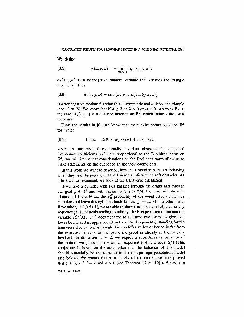
We define

co*51 ~A(x!Y,~) = -Bi(pfijloge~(.,~,w). z>

ax(z, y,w) is a nonnegative random variable that satisfies the triangle inequality. Thus,

(0.6) ~A(z, Y, w> = max(ax(2, Y, w>, Q(Y, 2, ~1) is a nonnegative random function that is symmetric and satisfies the triangle inequality [8]. We know that if d 2 3 or X > 0 or w $ 0 (which is P-a.s. the case) dx(-, ., w) is a distance function on I@, which induces the usual topology.

From the results in [6], we know that there exist norms ox(.) on Wd for which

(O-7) P-a.s. &CO, y, w> - ax(~) as Y -+ 00,

where in our case of rotationally invariant obstacles the quenched Lyapounov coefficients ax(.) are proportional to the Euclidean norm on Rd, this will imply that considerations on the Euclidean norm allow us to make statements on the quenched Lyapounov coefficients.

In this work we want to describe, how the Brownian paths are behaving when they feel the presence of the Poissonian distributed soft obstacles. As a first critical exponent, we look at the transverse fluctuation:

If we take a cylinder with axis passing through the origin and through our goal y E Wd and with radius 1~17, y > 3/4, then we will show in Theorem 1.1 that lP-a.s. the @-probablity of the event A(y, y), that the 1 path does not leave this cylinder, tends to 1 as 1yI --+ 00. On the other hand, if we take y < l/(d+ l), we are able to show (see Theorem 1.3) that for any sequence (y,), of goals tending to infinity, the E-expectation of the random variable pp [A(y,, r)] d oes not tend to 1. These two estimates give us a lower bound and an upper bound on the critical exponent E, standing for the transverse fluctuation. Although this subdiffusive lower bound is far from the expected behavior of the paths, the proof is already mathematically involved. In dimension d = 2, we expect a superdiffusive behavior of the motion, we guess that the critical exponent < should equal 2/3 (This conjecture is based on the assumption that the behavior of this model should essentially be the same as in the first-passage percolation model (see below). We remark that in a closely related model, we have proved that [ > 3/5 if d = 2 and X > 0 (see Theorem 0.2 of [lo])). Whereas in

Vol. 34, no 3-1998.

282 M. V. WijTHRICH

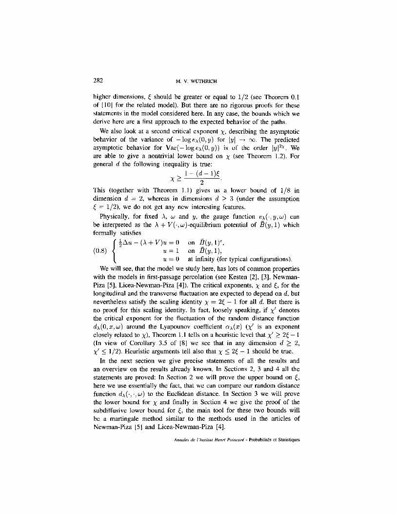
higher dimensions, < should be greater or equal to l/2 (see Theorem 0.1 of [lo] for the related model). But there are no rigorous proofs for these statements in the model considered here. In any case, the bounds which we derive here are a first approach to the expected behavior of the paths.

We also look at a second critical exponent x, describing the asymptotic behavior of the variance of - log ex(O, y) for Iy] ----t 0~). The predicted asymptotic behavior for Var(- logex(0, y)) is of the order ]y12X. We are able to give a nontrivial lower bound on x (see Theorem 1.2). For general d the following inequality is true:

X2 1 - (d - l)<

2 ( This (together with Theorem 1.1) gives us a lower bound of l/8 in dimension d = 2, whereas in dimensions d 2 3 (under the assumption < = l/2), we do not get any new interesting features.

Physically, for fixed A, w and y, the gauge function ex(., y,w) can be interpreted as the X + V(,, w)-equilibrium potential of B(y, 1) which formally satisfies

1

$Au - (X + V)u = 0 on B(y: l)“,

(0.8) u = 1 on B(y, l), u=o at infinity (for typical configurations).

We will see, that the model we study here, has lots of common properties with the models in first-passage percolation (see Kesten [2], [3], Newman- Piza [5], Licea-Newman-Piza [4]). The critical exponents, x and <, for the longitudinal and the transverse fluctuation are expected to depend on d, but nevertheless satisfy the scaling identity x = 2E - 1 for all d. But there is no proof for this scaling identity. In fact, loosely speaking, if x’ denotes the critical exponent for the fluctuation of the random distance function dx (0,x, w) around the Lyapounov coefficient QX(X) (x’ is an exponent closely related to x), Theorem 1.1 tells on a heuristic level that x’ > 2[ - 1 (In view of Corollary 3.5 of [8] we see that in any dimension d > 2, x’ 5 l/2). Heuristic arguments tell also that x 5 2{ - 1 should be true.

In the next section we give precise statements of all the results and an overview on the results already known. In Sections 2, 3 and 4 all the statements are proved: In Section 2 we will prove the upper bound on {, here we use essentially the fact, that we can compare our random distance function dx(., ., w) to the Euclidean distance. In Section 3 we will prove the lower bound for x and finally in Section 4 we give the proof of the subdiffusive lower bound for <, the main tool for these two bounds will be a martingale method similar to the methods used in the articles of Newman-Piza [5] and Licea-Newman-Piza [4].

Annales de I’hstirut Henri PoincarP F’robabilit6s et Statistiques

FLUCTUATION RESULTS FOR BROWNIAN MOTION IN A POISSONIAN POTENTIAL 283

1. SETTINGS AND RESULTS

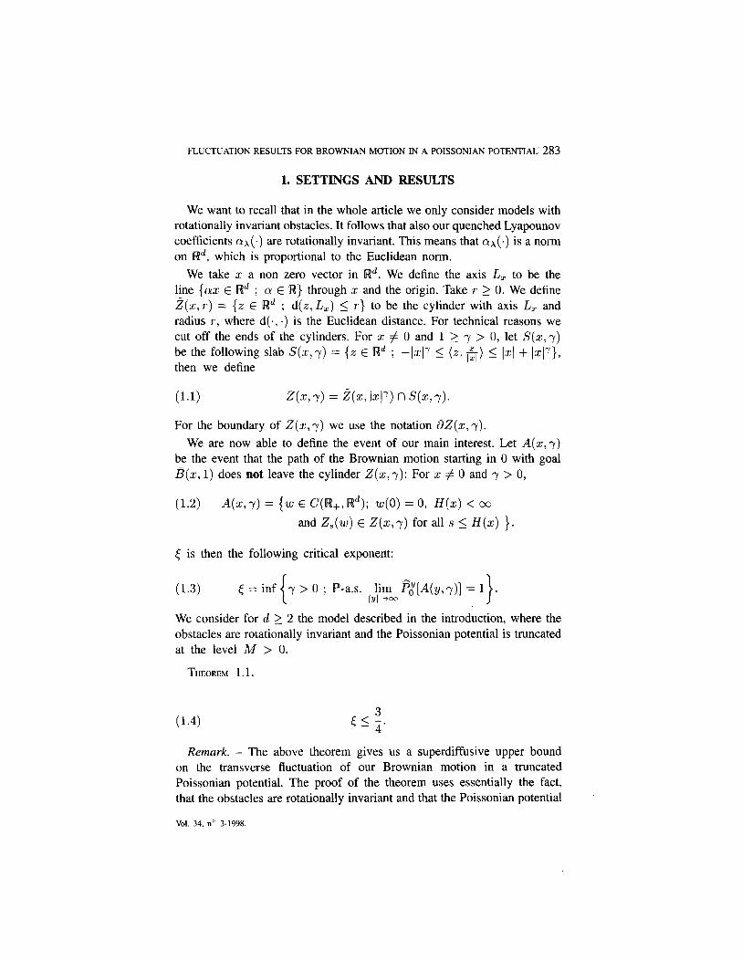
We want to recall that in the whole article we only consider models with rotationally invariant obstacles. It follows that also our quenched Lyapounov coefficients o X(.) are rotationally invariant. This means that a~(.) is a norm on Wd, which is proportional to the Euclidean norm.

We take z a non zero vector in Rd. We define the axis L, to be the line {CYX E Rd J (u E Iw} through z and the origin. Take T 2 0. We define Z(z,r) = (2 E Rd ; d(z, L,) 5 r} to be the cylinder with axis L, and radius T, where d(., .) is the Euclidean distance. For technical reasons we cut off the ends of the cylinders. For z # 0 and 1 2 y > 0, let S(s, y) be the following slab S(z, y) = {z E Rd ; then we define

-I$ I (23 6) I 14 + I@19

For the boundary of 2(x, y) we use the notation dZ(z, y).

We are now able to define the event of our main interest. Let A(z; y) be the event that the path of the Brownian motion starting in 0 with goal B(z, 1) does not leave the cylinder 2(x, y): For z # 0 and y > 0,

(1.2) A(z,r) = {w E C(IW+,Wd); w(0) = 0, H(z) < cc

and Z,(w) E Z(X,Y) for all s < H(z) }.

< is then the following critical exponent:

(1.3) y > 0 ; lP-a.s. ,vl,iim, @[A(y, y)] = 1

We consider for d > 2 the model described in the introduction, where the obstacles are rotationally invariant and the Poissonian potential is truncated at the level M > 0.

THEOREM 1.1.

(1.4) EL ;.

Remark. - The above theorem gives us a superdiffusive upper bound on the transverse fluctuation of our Brownian motion in a truncated Poissonian potential. The proof of the theorem uses essentially the fact, that the obstacles are rotationally invariant and that the Poissonian potential

Vol. 34, no 3-1998.

284 ha. v. WUTHRICH

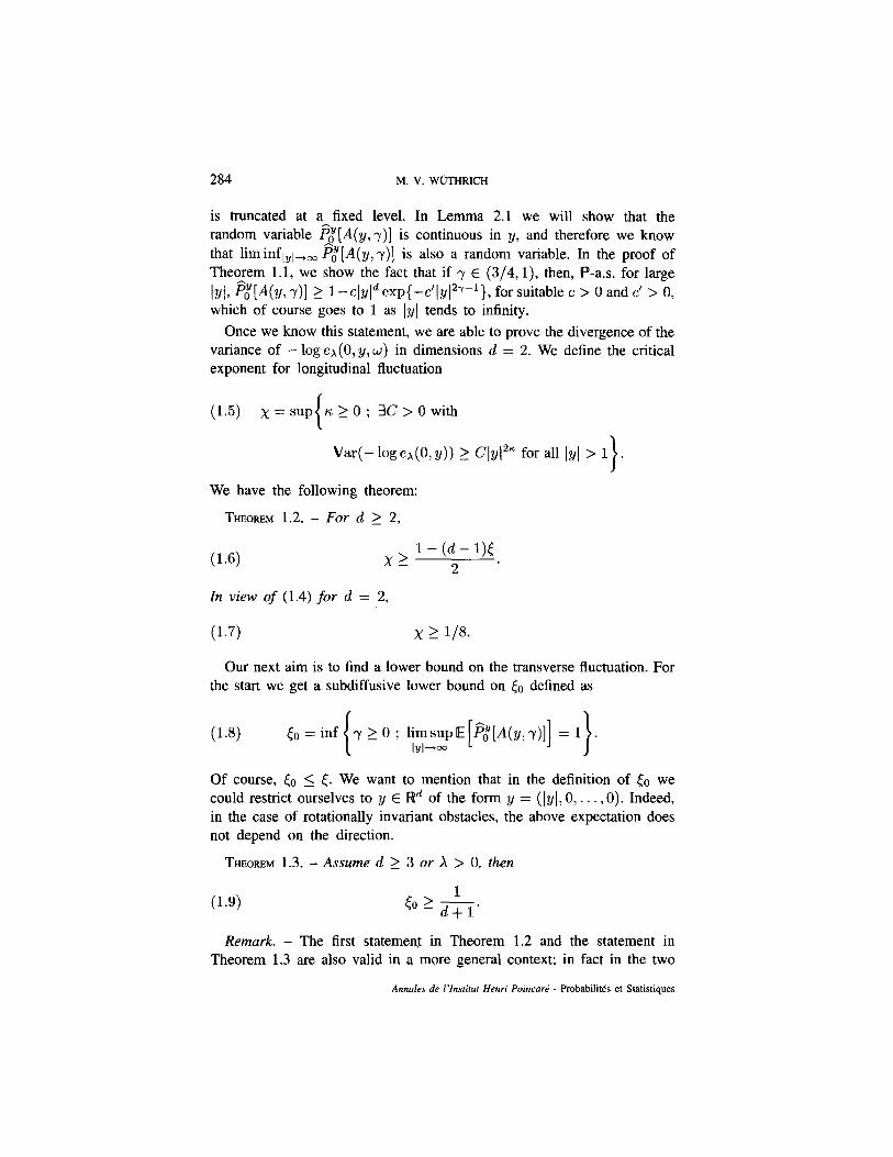
is truncated at a fixed level. In Lemma 2.1 we will show that the random variable c{[A(y, r)] is continuous in y, and therefore we know that liminfl,l,, P,Y[A(Y,Y)] is also a random variable. In the proof of Theorem 1.1, we show the fact that if y E (3/4, l), then, P-a.s. for large (y], @‘[A(y, r)] 2 1 -c]yld exp{ -c’]y]2y-1}, for suitable c > 0 and c’ > 0, which of course goes to 1 as ] y ] tends to infinity.

Once we know this statement, we are able to prove the divergence of the variance of - log ex(O, y, w) in dimensions d = 2. We define the critical exponent for longitudinal fluctuation

(1.5)

Var(-logex(O,y)) 2 C]y12” for all ]y] > 1 . >

We have the following theorem:

THEOREM 1.2. - For d 2 2,

(1.6) x >_ 1 - Cd - 1X

2 4

In view of (1.4) for d = 2,

(1.7) x L l/8.

Our next aim is to find a lower bound on the transverse fluctuation. For the start we get a subdiffusive lower bound on [a defined as

(l-8) <o = inf i

y 2 o ; l~yzip~ pl[A(y, r)]] = 1 I

.

Of course, <a < c. We want to mention that in the definition of cc we could restrict ourselves to y E Wd of the form y = (]y], 0, . . . , 0). Indeed, in the case of rotationally invariant obstacles, the above expectation does not depend on the direction.

THEOREM 1.3. - Assume d 2 3 or X > 0, then

(1.9) EOLL. d+l Remark. - The first statement in Theorem 1.2 and the statement in

Theorem 1.3 are also valid in a more general context; in fact in the two

Ann&s de l’htifuf Henri PoincorP - F’mbabiWs et Statistiques


proofs we do not use that the shape function is rotationally invariant. We only require this assumption in the proof of Theorem 1.1 and as a consequence for the lower bound on x in dimension d = 2.

We sometimes use the terminology of first-passage percolation because the situation in the case of Brownian motion in a truncated Poissonian potential looks very similar. In first-passage percolation, to prove the statements one has often (unverified) assumptions on the curvature of the asymptotic shape, here we do not have these problems because in the case of rotationally invariant obstacles one knows that the asymptotic shape is a ball with positive radius. This fact indicates an advantage of our model.

To close this chapter we give some further general notations and state some already known results we will need later on. We usually denote positive constants by cl, c2, . . . and yr, 7~~ . . . . These constants will only depend on the invariant parameters of our model, namely the dimension d, the intensity V, the shape function W, the truncation level A4 and the parameter X. The constants which are used in the whole article are denoted by yi, whereas ci is only used for local calculations in the proofs.

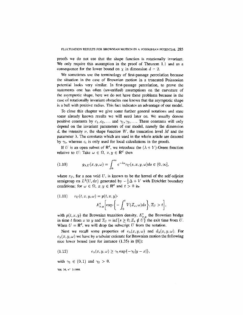
If U is an open subset of Wd, we introduce the (A + V)-Green function relative to U: Take w E R, z,y E Rd then

(1.10) gx,Lr(x, y, w) = s m e-xsm(s,x, y, w)ds E C&4, 0 where rt~, for a non void U, is known to be the kernel of the self-adjoint semigroup on L2( U, dz) generated by - iA + V with Dirichlet boundary conditions; for w E 0, x, y E Wd and t > 0 is.

(1.11) ru(t, x, y, w) = P(kX! Y>- t V(&,w)ds

I I ,Tu > t ,

with p(t, z, y) the Brownian transition density, ES,, the Brownian bridge in time t from z to y and Tu = inf{s > 0; 2, 4 U} the exit time from U. When U = Wd, we will drop the subscript U from the notation.

Next we recall some properties of ex(xc, y, w) and dx(x, y, w). For ex(x, y, w) we have by a tubular estimate for Brownian motion the following nice lower bound (see for instance (1.35) in [S]):

(1.12) ex(x:,Y,w) 2 71 exp{-y2ly - 41,

with y1 E (0,l) and ry2 > 0.

Vol. 34. no 3-1998.

286 M. v. W.~THRICH

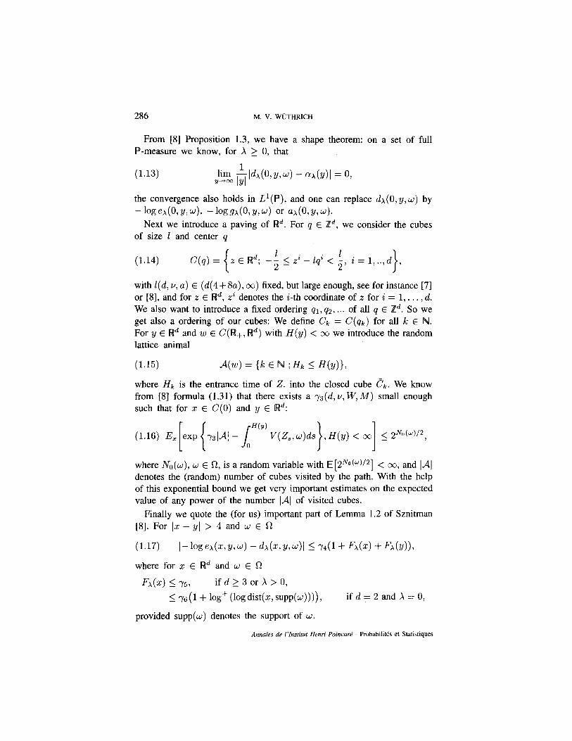
From [8] Proposition 1.3, we have a shape theorem: on a set of full P-measure we know, for X 2 0, that

(1.13)

the convergence also holds in L1 (P), and one can replace dx(O, y, w) by - logex(O, Y,w)~ - loggx(O,~,w) or ~(0, Y,w).

Next we introduce a paving of Rd. For Q E Zd, we consider the cubes of size 1 and center q

(1.14) 1

-; 5 zi -lqi < 2, i = l,..,d >

,

with Z(d, V, u) E (d(4+8a), oc) fixed, but large enough, see for instance [7] or [8], and for z E I@, zi denotes the i-th coordinate of .z for i = 1,. . . , d. We also want to introduce a fixed ordering ql, q2, ,.. of all q E Zd. So we get also a ordering of our cubes: We define C, = C(qk) for all Ic E N. For y E Rd and w E C(R+, R”) with H(y) < oe we introduce the random lattice animal

(1.15) d(w) = {k E N r IJk 5 H(Y)),

where Hk is the entrance time of 2. into the closed cube ck. We know from [8] formula (1.31) that there exists a y3(d, V, W, M) small enough such that for x E C(0) and y E Rd:

(1.16) &[exp { ys,d,- ~H’y)V(Zs,w)dJ).H(y) < co] I 2No(w)/2,

where No(w), w E Q is a random variable with E [2h’o(w)/2] < m, and IAl denotes the (random) number of cubes visited by the path. With the help of this exponential bound we get very important estimates on the expected value of any power of the number IAl of visited cubes.

Finally we quote the (for us) important part of Lemma 1.2 of Sznitman [S]. For IZ - y[ > 4 and w E R

(1.17) I-loge~(x,y,w) - dx(x,y,w)l 5 74(1+ Fx(x) i- FxlY)h

where for x E Wd and w E R

FA(X) 575, if d 2 3 or X > 0,

L -YG (1 + log+ (log dist(x, supp(w)))), if d = 2 and X = 0,

provided supp(w) denotes the support of w.

Ann&s de I’hsritut Hewi Poincm! F’robabilit& et Statistiques


2. PROOF OF THE SUPERDIFFUSIVE UPPER BOUND ON [

First we start with a continuity result. We want to show that the limit in the definition of [ is a well-defined random variable. Therefore we have to show that @[A(y, y)] is continuous in y.

LEMMA 2.1. - For X 2 0 and y > 0, thefunctions (y, w) + ex(O, y, U) and

(Y> w> --+ &W(~/dl are measurable in w and for all IyI > 1 continuous in y.

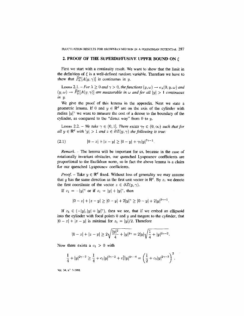
We give the proof of this lemma in the appendix. Next we state a geometric lemma. If 0 and y E Rd are on the axis of the cylinder with radius ]yly we want to measure the cost of a detour to the boundary of the cylinder, as compared to the “direct way” from 0 to y.

LEMMA 2.2. - We take y E (0, 11. There exists y7 E (0, CXI) such that for all y E Wd with IyyI > 1 and z E dZ(y, y) the following is true:

(2.1) IO - ZJ + I.2 - YI 2 IO - YI + Y71Y12y-1.

Remark. - The lemma will be important for us, because in the case of rotationally invariant obstacles, our quenched Lyapounov coefficients are proportional to the Euclidean norm, so in fact the above lemma is a claim for our quenched Lyapounov coefficients.

Proof - Take ‘y E Rd fixed. Without loss of generality we may assume that y has the same direction as the first unit vector in Rd. By z1 we denote the first coordinate of the vector z E dZ(y, 7).

If zi = -(y]Y or if zr = ]y] + (y]Y, then

10 - z( + Iz - yl > IO - f/J + 21Y17 L IO - YI + 21y12y-1e

If 21 E (-IYLIYI + Ivl-9, th en we see, that if we embed an ellipsoid into the cylinder with focal points 0 and y and tangent to the cylinder, that IO - 4 + Iz - Yl is minimal for zi = ]y]/2. Therefore

lo-4+l~-Ylr2 TflYl -2lYl 4flYl -. /w-T- f-75

Now there exists a cl > 0 with

a + IYI 2-v-2 2 a + cllyp2 2

+Glyl - 4-r-4 -

( ; + clly127-2 .

>

vol. 34. Ilo 3-1998.

288 M. V. WijTHRICH

So we see that

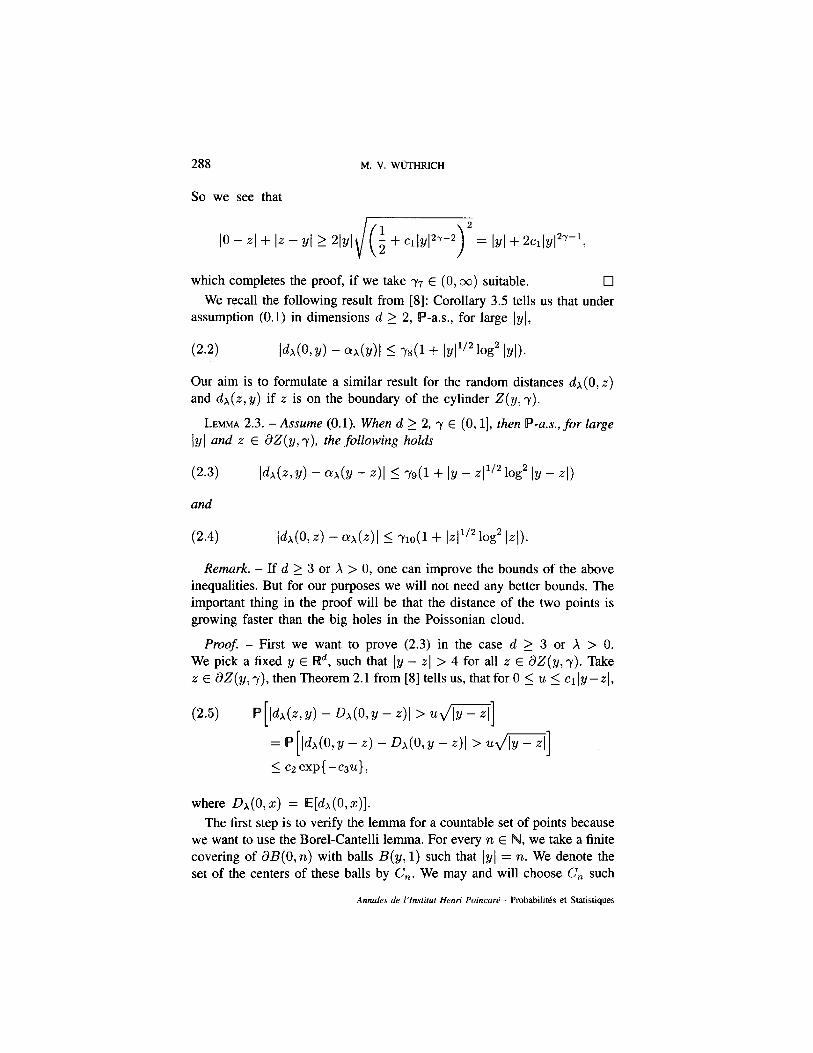
IO - 4 + Iz - Yl 2 2lYl /(f + .,ly127-92 = lyl + 2clly127--1,

which completes the proof, if we take 77 E (0, cc) suitable. 0 We recall the following result from [8]: Corollary 3.5 tells us that under

assumption (0.1) in dimensions d 2 2, IP-a.s., for large Iy],

(2.2) IW,d - ax(Y)1 5 78(1 + 1~1~‘~ log2 1~1).

Our aim is to formulate a similar result for the random distances dx(O, z) and dx (z, y) if z is on the boundary of the cylinder Z(y, y).

LEMMA 2.3. - Assume (0.1). When d 2 2, y E (0, 11, then P-U.S., for large IyI und z E aZ(y, y), the following holds

(2.3) Idx(z, y) - W(Y - 41 5 ~(1 + IY - ~1~‘~ log2 IY - 4)

and

P-4) I&(0,4 - 441 5 ym(l + 1~1~‘~ log2 1~1).

Remark. - If d 2 3 or X > 0, one can improve the bounds of the above inequalities. But for our purposes we will not need any better bounds. The important thing in the proof will be that the distance of the two points is growing faster than the big holes in the Poissonian cloud.

Proof. - First we want to prove (2.3) in the case d 2 3 or X > 0. We pick a fixed y E Rd, such that Iy - z] > 4 for all z E dZ(y, y). Take z E aZ(y, r), then Theorem 2.1 from [8] tells us, that for 0 5 u 5 cl/y-z],

(2.5) P[lW,y) - ~(O,Y - 41 > w/‘y-Fi]

= $ [l&(0, y - z) - &CO, Y - z>I > m/‘ji?l] 5 ~2 ew{-w),

where &(0,x) = E[dx(O,z)].

The first step is to verify the lemma for a countable set of points because we want to use the Borel-Cantelli lemma. For every n E N, we take a finite covering of aB(O, n) with balls B(y, 1) such that ]y] = n. We denote the set of the centers of these balls by C,. We may and will choose C, such

Ann&s de I’htirut ffenri Poincar6 - Probabilith et Statistiques


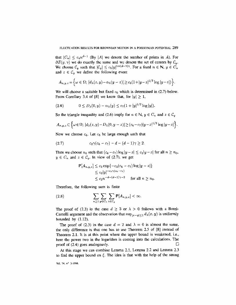
that IC,] 5 c&l (By IAl we denote the number of points in A). For dZ(y, 7) we do exactly the same and we denote the set of centers by C,. We choose C, such that ICYI 5 ~sly(l+(~-~)Y. For a fixed n E N, y E C, and z E C, we define the following event

A n,y,z= { w E Q; I&(Z,Y)-Qx(Y - z)l2C~~l+lY-rl”~lo~lY-zI~}.

We will choose a suitable but fixed cg which is determined in (2.7) below. From Corollary 3.4 of [8] we know that, for Iy( 2 1,

(2.6) 0 I Dx(O, Y) - @A(Y) I c7(1 + lYP2 1% IYlh

So the triangle inequality and (2.6) imply for n E N, y E C, and z E C,

A n,y,zc{wEfi; Idh(Z,y)-~X(0,y-Z)I~(c6-C7)ly-Z(1’210gIY--ZI}.

NOW We choose cs. Let cs be large enough such that

(2.7) c3”)‘(c6 - CT) - d - (d - l)r 1 2.

Then we choose no such that (cc - c7) log )y - z] 5 clly - z] for all n 2 no, y E C, and z E C,. In view of (2.7), we get

Wn,y,z] I cz exp{-cdc6 - CT) log (Y - 4) 5 c21ypY(c6--c7)

< C2n-w-lh-2 - for all n > no.

Therefore, the following sum is finite

The proof of (2.3) in the case d 2 3 or X > 0 follows wi,th a Borel- Cantelli argument and the observation that supI,-yII1 dx(z, y) is uniformly bounded by (1.12).

The proof of (2.3) in the case d = 2 and X = 0 is almost the same, the only difference is that one has to use Theorem 2.5 of [g] instead of Theorem 2.1. It is at this point where the upper bound is weakened, i.e., here the power two in the logarithm is coming into the calculations. The proof of (2.4) goes analogously. cl

At this stage we can combine Lemma 2.1, Lemma 2.2 and Lemma 2.3 to find the upper bound on S. The idea is that with the help of the strong

Vol. 34, no 3-1996

290 M. V. WUTHRICH

Markov property and the above lemmas one sees that the detour over the boundary of the cylinder costs too much.

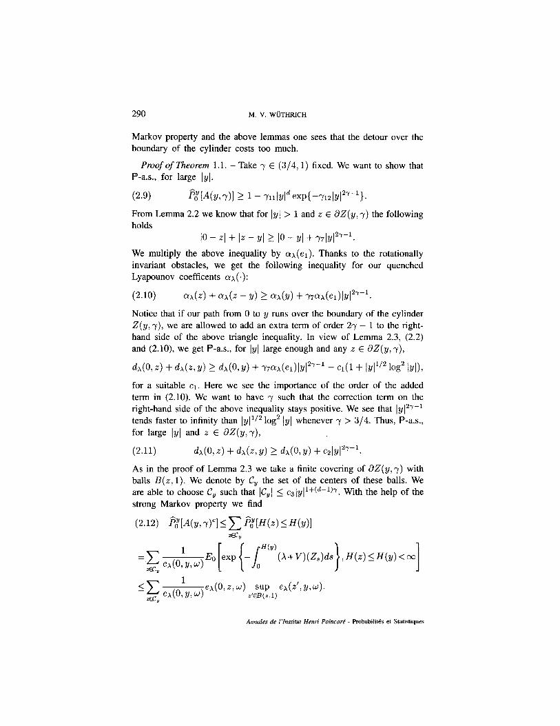
Proof of Theorem 1.1. - Take y E (3/4,1) fixed. We want to show that P-a.s., for large jyl,

P-9) @iMy, r)] 2 1 - mbld evi-mly12Y-1~.

From Lemma 2.2 we know that for IyI > 1 and z E dZ(y, y) the following holds

IO - 4 + lz - YI 2 IO - Yl + Y71Y127-1. We multiply the above inequality by aA( Thanks to the rotationally invariant obstacles, we get the following inequality for our quenched Lyapounov coefficents QX (.):

(2.10) a(~> + QA(~ - Y) 2 ax(~) + ~7~~(el)ly12Y-1.

Notice that if our path from 0 to y runs over the boundary of the cylinder Z(y, y), we are allowed to add an extra term of order 27 - 1 to the right- hand side of the above triangle inequality. In view of Lemma 2.3, (2.2) and (2.10), we get P-a.s., for IyI large enough and any z E dZ(y,r),

&CO, z) + &(z, Y) 2 &(O, Y) + vax(el)ly12Y-1 - ~(1 + lyll’* log* Ivl>,

for a suitable cl. Here we see the importance of the order of the added term in (2.10). We want to have y such that the correction term on the right-hand side of the above inequality stays positive. We see that IYI*Y-~ tends faster to infinity than ly/l/* log* IyI whenever y > 3/4. Thus, P-a.s., for large IyJ and z E dZ(y, y),

(2.11) &(O, 2) + dx(z, Y) 2 dx(O, Y) + C2lYl 27-l

.

As in the proof of Lemma 2.3 we take a finite covering of aZ(y, y) with balls B(z, 1). We denote by C, the set of the centers of these balls. We are able to choose C, such that IC,I 5 es lyll+(d-l)y. With the help of the strong Markov property we find

1 H(Y)

= c g ex(O,y,w)

(~+V)(Zs)~s 3 H(z) I H(Y) <cc Y 1 ex(O, z, w> sup ex(z’, y, w).

z’cB(z,l)

Andes de l’htituf Hem-i Poinc& Probabilith et Statistiques


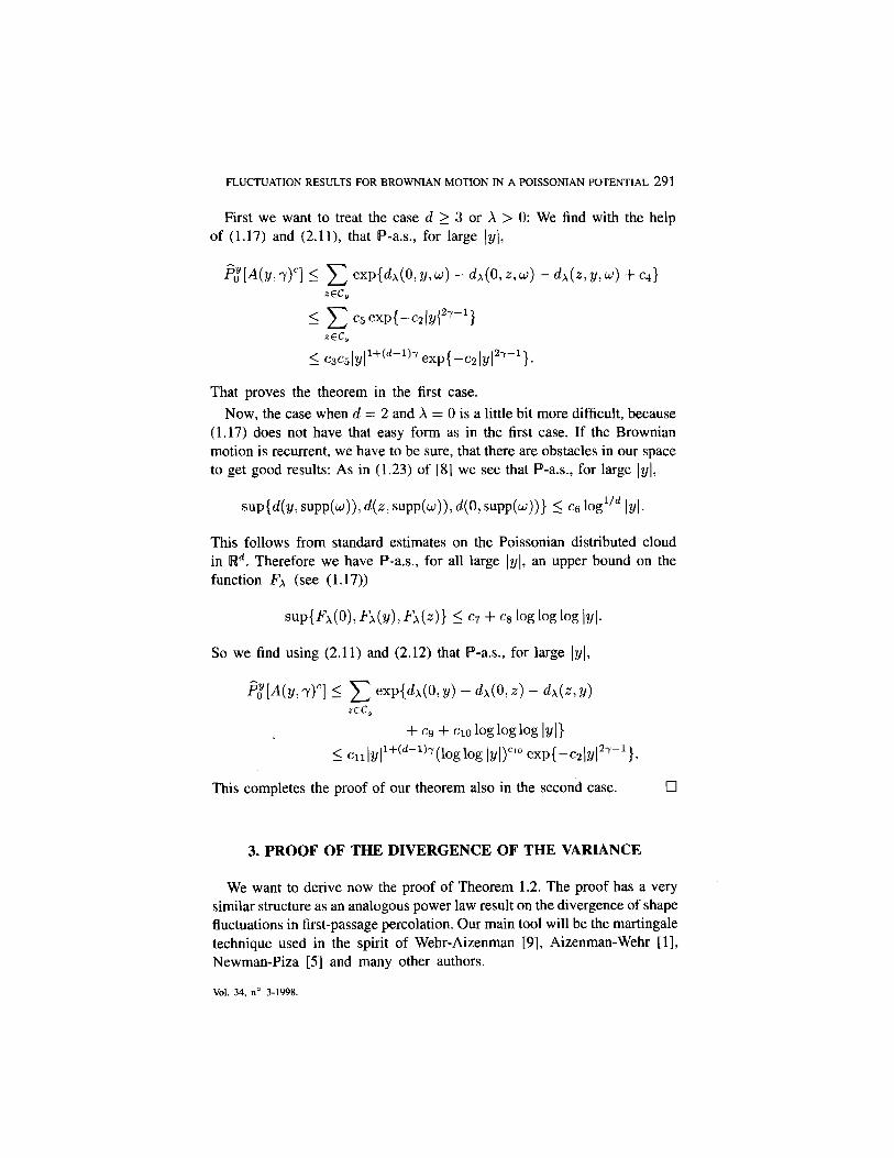
First we want to treat the case d 2 3 or X > 0: We find with the help of (1.17) and (2.11), that P-a.s., for large (y],

pt[A(y, y)‘] 5 c exp{dx(O, Y, u) - dx(O, 2,~) - dx(Z, y,w) + ~43

ZEC,

I c c5 exp{-c21y12Y-1)

ZEC,

5 q~~Jyl~+(~-~)~ exp{-c21y(2Y-1}.

That proves the theorem in the first case. Now, the case when d = 2 and X = 0 is a little bit more difficult, because

(1.17) does not have that easy form as in the first case. If the Brownian motion is recurrent, we have to be sure, that there are obstacles in our space to get good results: As in (1.23) of [8] we see that P-a.s., for large Iy],

wW, s~PP(w>>> 4 z, SUPP(W)), 40, SUPPW} 5 cc 10g”~ IYI.

This follows from standard estimates on the Poissonian distributed cloud in Rd. Therefore we have P-a.s., for all large Jy], an upper bound on the function FA (see (1.17))

sup{F~(O), FA(Y), W>) L ~7 + cs loglogk IYI.

So we find using (2.11) and (2.12) that P-a.s., for large 1~1,

p{[A(y, y)“] 5 c exp{dx(O, y) - dx(O, 2) - dx(z, Y) ZEC,

+ c9 + Cl0 logloglo!s IYII 5 clllyll+(d-l)Y(loglog ]yl)“‘” exp{-c2Jy12y-1}.

This completes the proof of our theorem also in the second case. cl

3. PROOF OF THE DIVERGENCE OF THE VARIANCE

We want to derive now the proof of Theorem 1.2. The proof has a very similar structure as an analogous power law result on the divergence of shape fluctuations in first-passage percolation. Our main tool will be the martingale technique used in the spirit of Wehr-Aizenman [9], Aizenman-Wehr [l], Newman-Piza [5] and many other authors.

Vol. 34, no 3-1998.

292 M. V. WijTHRICH

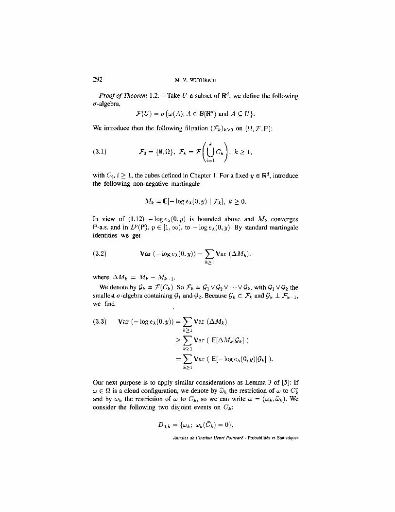
Proof of Theorem 1.2. - Take U a subset of Rd, we define the following u-algebra,

F(U) = a{w(A); A E o(Rd) and A C U}.

We introduce then the following filtration (.?-k)kza on (R,7, P):

(3.1) 30={0,R}, 3k=3 (JCk ( )

7 kZ1, i=l

with Ci, i > 1, the cubes defined in Chapter 1. For a fixed y E Wd, introduce the following non-negative martingale

Mk = E[-kex(O,y) 1 Fk], k 2 0.

In view of (1.12) - log ex (0, y) is bounded above and Mk converges P-as. and in P(P), p E [l, co), to - logex(0, y). By standard martingale identities we get

(3.4 Var (-logex(O,y)) = Char (AMk), k>l

where Ahl, = I%!fk - iV?k-1.

We denote by 91, = 3(Ck). So 3k = 91 V 82 V *. * V &, with 6% V 6?i? the smallest a-algebra Containing 41 and &. Because GI, C 3k and &?I, 1 3k-1,

we find

(3.3) Var (- logex(O, y)) = x Var (AMk) k>l

= xvar ( E[-logex(O,y)l~k] >.

k>l

Our next purpose is to apply similar considerations as Lemma 3 of [.5]: If w E fl is a cloud configuration, we denote by i& the restriction of w to Ci and by wk the restriction of w to Ck, so we can write w = (Wk, ijk). We consider the following two disjoint events on ck:

DO,k = {wk; wk@k) = o},

Ann&s de I’hsritut Henri Poincarc! - Pmbabilit& et Statistiques


this is the event that the cube C?k receives no point of the cloud. Whereas

Dl,k = {Wki Wk(qlk, 1)) 2 1)

is the event that we have at least one point of the Poissonian cloud in the center (i.e., in the closed ball with center Zqk and radius 1) of the cube C,. We then define, for S = 0 or 1,

Df = {W E fl with wk E Da,k}.

Of course, DE and 0: are disjoint and Gk measurable. We denote by p = P”[Di] > 0 and by q = P[Dk] > 0.

E[- log ex(O, Y, w>lGkl * 10; (WI = E[-logex(O,y,w)lD~(W)l~kl

analogously one gets the following lower bound

We remark that

sup inf {c; EDa,kl

-logex(O,y,(&-1) and (o:EDIk~-loge~(O,~,(~:,.))

are measurable. This can be seen by using an approximation of the cloud configuration by cloud configurations with rational coordinates. We define z. and zr as follows,

x0 =

E[E[-~~ex(O,Y~w)lBkl~lq(~)]

WI

-l%eA(o,Y,(&~k)) , 1 Vol. 34, no 3-1998.

M. V. WiSTHRICH 294

and

Xl = E [EL- log ex(O, Y, ~)lGkl . 10; (w)]

W;l >E [

inf - log ex(O, Y, (a:, Gk)) . (T;EDl,k 1

To simplify the notation we introduce:

In view of the above bounds on x0 and xl, we see that x1 -x0 2 E[Ek] 2 0 and therefore

(3.4) (Xl - xoy 2 E[Ek12.

Using Lemma 3 of [5], we have the following estimate

Var ( E[-logedodgkl > 2

Therefore, together with (3.3) and (3.4), this is yielding a lower bound for the variance of - log ex (0, y)

Take y > E and define Eli = {Ic E N with ck il Z(y,y) # @}, to be all the cubes, that intersect the cylinder Z(y, y) with radius ]y]Y. We know that l&l 5 cllvl l+(d-l)y for a suitable cl E (0, oo). With the help of Cauchy-Schwarz inequality, we get

Ann&s de l’lnstitut Henri Poincarti Robabilith et Statistiques


If we are able to prove that there exists a cg E (0, oc) with

(3.6)

then x 2 (1 - (d - l)y)/2 f or all y > <, so the claim of Theorem 1.2 follows for d 2 2, whereas for the bound l/8 for d = 2 one simply inserts the bound for [ given in Theorem 1.1. It remains to prove (3.6).

We will therefore prove two technical lemmas, the proof of the two lemmas will essentially be the same as the proof of formulas (2. lo), (2.11) and (2.13) of [8]: For k 2 1, take 0: E DS,k, with S = 0 or 1, w E R and z E Rd. We define the potential (3.7)

v,s(x,i&) = kf A W(x - ~)d#/) + s w(x - y)&(dy) c; If C’I, is the closed u-neighborhood of Ck, then notice that

(3.8) VL = Vj on CL and vi >v:onCk,

and there exists a c4 > 0 and a domain G C CI, (depending on ai E Di,k) such that G has positive Lebesgue measure and the difference Vi - I$’ > c4 on G. Define fik = Hek to be the entrance time of 2. into Ck, and Hk = Hc, to be the entrance time of 2. into the closed cube Ck. So we denote the path measure on C(R+, Rd) generated by V,,f with start in x E Rd and goal in y E Wd as follows

1

= eX(x,Y,g&Gk)

H(Y)

(A + %%&>ds l{H(y)<+%

to ‘avoid overloaded notations we will drop the brackets for the cloud configuration in the gauge function.

LEMMA 3.1. - With the above notations the following statements are true:

and

Vol. 34. II” 3-1998.

296 M. V. WmHRICH

Proof of the lemma. - With the help of the strong Markov property follows

Whereas for the second claim of the lemma one has to exchange the role of c: and 0:. This finishes the proof of Lemma 3.1. cl

The second lemma tells us, how to handle the fraction on the right-hand side of the equation in the above lemma. For k 2 1, take U: E Da,k, with 6 = 0 or 1, w E R and y E Rd, we denote by $$(., .) the (A + Vi)-Green function on U = B(y, l)“, that is, for 2, z E &,

see also formula (1 .lO).

LEMMA 3.2. - With the above notations the following two statements are

= J _ sZ:X(c ~><Vi - V,O)(z)ex(z, y, &Gk)dZ. Ck

Proof of the lemma. - By a classical differentiation and integration argument one has for w E C(W+,Rd), with H(y) < 00,

H(Y)

=1+ /“‘y)(V~ - Vf)(Z,) exp - /H’y’(Vt - VL)(Zu)du ds. 0 s

To prove the first claim, we multiply both sides by

H(Y)

(A + V,‘>(Zs>ds

Ann&s de I’lnsfirut ffenri P&car6 - Probabilitks et Statistiques


and take the integration with respect to ljH(y)<m}Pz. Whereas for the second claim one has to exchange the role of a: and 0:. This finishes the proof of Lemma 3.2. 0

Now we are able to prove (3.6). Take ai E Da,k. (In fact DO,k contains only one element.) Then

(3.10) -J&(0, y, G) = inf - log u;aA.le (

e&4 y, &Gk) eX(O,y,a~,w^k) >

> o - ’

We want to find a good lower bound on the term on the right-hand side of the above equation. We take a fixed cr: E Di,h. Then by Lemma 3.1 and Lemma 3.2 we find

- log (

ex(O,y,d,Gk) ex(O,y,&Gk) >

= -log 1 + E,“>” ( [

I-r,, < H(y), eX(Zfik7Y,&Gk) _ 1

ex(Zfi,, Y, a:, Gk) I>

= -log (1- @“[fi, 5 H(y),

J . _

Ck I) Now, we have to distinguish whether ek is a neighboring box of our goal or not: Choose R minimal, such that ck C B(&, R). we say tik is a neighboring box of y E Rd if y is contained in the closure of B( lq,+, R + 2). Define

NV = {

k E N; C$ is a neighboring box of y >

.

Of course the number of points contained in NY is bounded by a constant only depending on a, 1 and d.

First case, k E NY.

Second case, k 4 NY. From Hamack’s inequality (see for instance [6] after (1.28)), we get, for k 2 1,

(3.11)

Vol. 34. no 3-1998

298 M. V. WUTHRICH

Thus, because (Vi - V,“)(z) > 0 we see that

>_ c,~~~o & I H(Y), J

_ Ck

&$xZfik 7 w,’ - b%)d~ I

>_ c&o [ IT, 5 H(y),

s S$(Z& 7 4(V, - V,O)(W .

Ck I

On k 4 N9, there exists a cs > 0, independent of k, such that for all z E 86’k and all rr: E Dr,k,

Therefore, we find

2 c7po -live [fik 5 H(y)].

If we insert this result into formula (3.10), we get

&(O, y,tlk) = inf - log U; Eh,k

where we have used Lemma 3.3 which follows below. Thus, we find the following lower bound

0 (3.12)

if k E NY c7@[Hk 5 H(y)] if Ic q! NY ’

If A(y, y) again denotes the event that the path of the Brownian motion starting in 0 with goal B(y, 1) does not leave the cylinder Z(y) r), we know,


because we have taken 7 > E, that BP-a.s. liminfl,l,, po[A(y, r)] = 1. Therefore,

> c7E IYI

~,W~~~412~;11 1 for all large 1~1.

So the claim (3.6) follows by the lemma of Fatou, this completes the proof of our theorem. q

LEMMA 3.3. - Take y E Rd, k > 1, w E at, gg E Da,k and 0: E Dl,k. Then we have

and

(3.14)

Proof. - We know by (3.8) that vf(ijk) < v,‘(&) and also vt(ijl,) 5 V(w). Therefore it suffices to prove the first claim, the second one then follows analogously. Let us define for S = 0, 1, w E C(R+, Wd),

H(Y) f(Gk,&w) = exp (A + v,S)(-%,‘+ ’ l{H(y)<cc}>

and observe that

(3.15) f(Gk, &w) . 1 {Eib>H(y)} = fh ‘% w> . ‘{&>H(y)]

(3.16)

Vol. 34, no 3-1998.

300 M. V. WUTHRICH

Therefore by (3.15) and (3.16) we get

Fo”,l [a I H(Y)]

Eo ZZ [ f(GddG4. l{&gqy)} 1 Eo f(&, a:> w> . ~mAH(?/)l + hk4w~ >I

This completes the proof of the lemma. Cl

4. PROOF OF THE SUBDIFFUSIVE LOWER BOUND OF to

The strategy of the proof of Theorem 1.3 is an extention of the arguments used in the proof of Theorem 1.2. For a similar result in first-passage percolation we want to refer to Section 3 of [4]. The idea of the proof is to compare - log ex (a, .) for the two different starting points 0 and m and the two different endpoints y and y + m. One easily gets an upper bound on the variance of the difference of these two “passage times”: If the distance between 0 and m is of order ]y]Y then Var(-logex(O,y)+logex(m,y+m)) = O(]y]“‘). On the other hand we will get, by the methods presented in the preceding chapter, a lower bound of the form ~]y]l-(~-l)~. S o if we choose y, the power of the cylinder radius, smaller than l/(d + 1) we get a contradiction, to the two bounds mentioned above, this leads us to the claim of Theorem 1.3.

Proof of Theorem 1.3. - Assume that for a fixed y E [0, 11, there exists a sequence (y,), c Rd with Jyn] --+ cc such that

c4.q E pp[A(y,, y)]] --+ 1 as n ---f cc.

In fact, by rotation invariance of the obstacles, we can and will choose the sequence (y,), such that yn = ( ]yn I, 0, . . . , 0) for all n. We want to show that under these assumptions y 2 l/(d + 1).

Define, for w E R, n 2 1, the difference of an “upper” and a “lower” passage time as follows

Slogen = -logex(O,y,,w) - (-logex(m,,y,+m,,w)),

Ann&s de I’fnsfiruuf Henn’ Pohcart! - Pmbabilitds et Statistiques


where we choose m, E Rd as follows: m, = (0, ]m,(, 0,. . . ,O) points into the direction of the second coordinate axis, and ]m,] is minimal such that the two cylinders g(y,, ]yn]r + &l) and z(ylz, ]yn]Y + &I) + m, are disjoint. We remark that (m, ( 5 cl (yn 17 for all large n because of our choice of the sequence (y,),. Using the strong Markov property, we see that

By Hamack’s inequality (see (3.11)), one gets

- log ( eA(O, Yn)

ex(m, yn + m,) > 5 ~2 - logex(O,m,) - logex(3h + m,,y,),

analogously, by exchanging the role of the passage times,

- log (

ex(O, h) eA(m,, yn + mn) >

> -cz+logex(m,,O) -logex(yn,yn+mn).

Therefore the following estimate on ]S log epz ] holds,

I ( - log ei4(0, YJ ex(m,, yn + m,) >I

5 c2 - logeA(O, m,) - logex(yn + m,, yn)

- log ex(m,, 0) - log ex(h, Yn + m,).

In view of (1.12), we find a suitable constant es E (0, co) such that for all large n

(4.2) Var(Sloge,) _< c3)mnj2 5 ~fcs]y~/nJ~~.

Hence, we have found the desired upper bound on the variance of the difference of these two passage times. During the rest of the proof we try to show that one gets the following lower bound on the same variance:

(4.3) ,Var(S log e,) 2 ~~ly,l’-(~-~)~.

If we have verified those two bounds, we see that 27 >_ 1 - (d - 1)y from which our claim, y 1 l/(d + l), follows. It remains to find the lower bound (4.3) on the variance of the difference of the two passage times.

With the same notations as in the previous chapters, we get by martingale identities as before

(4.4) Var(Sloge,) > CVar( E[Sloge,(Sk] ). k>l

So we are again interested in a lower bound for Var( E[Sloge,]&] ). We introduce the same events &,k, &,k, @ and 0: on our cubes ck

Vol. 34, no 3-1998.

302 M. V. WijTHRICH

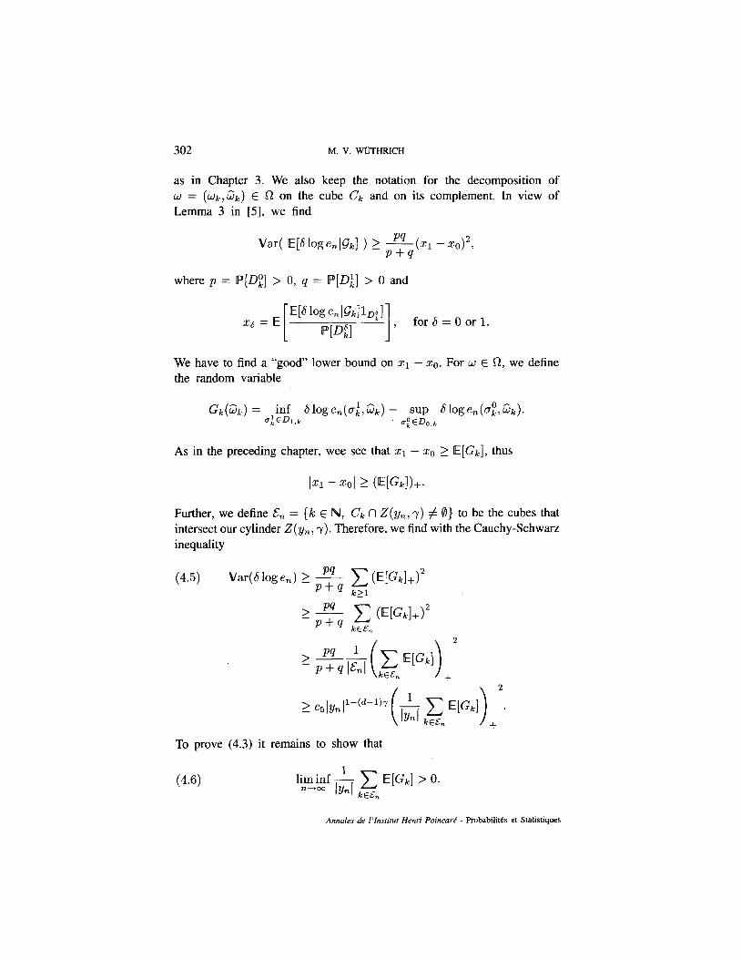
as in Chapter 3. We also keep the notation for the decomposition of w = (wk,&) E R on the cube Ck and on its complement. In view of Lemma 3 in [5], we find

Var( E[filoge,lGk] ) 2 -J&(51 - WOK

where p = P[DE] > 0, Q = P[DL] > 0 and

26 = E

[

WkenlGk]lD;] pLDfl

I , for S = 0 or 1.

We have to find a “good” lower bound on x1 - x0. For w E R, we define the random variable

As in the preceding chapter, wee see that x1 - x0 2 E[Gk], thus

Further, we define E, = {k E N, C’r, II Z(y,, 7) # 0) to be the cubes that intersect our cylinder 2 ( yn, 7). Therefore, we find with the Cauchy-Schwarz inequality

(4.5) Var( S log e,) 2

To prove (4.3) it remains to show that

(4.6)

FLUCTUATION RESULTS FOR BROWNIAN MOTION lh’ A POISSONIAN POTENTIAL 303

We denote the only element in Do,k by u:. For w E R is

+ inf - log ex(m,,y, + m,,oE,ljk) U:EDl.k ex(m,,y, +m,,&ijk)’

Thus, it suffices to prove

(4.7) ll,tEf & kEE, E c[ inf log 40,yn,~~,~k) ex(O, yn, &Gk) 1 , o

U:EDl>k ’

The proof of claim (4.7) follows exactly in the same way as the proof of (3.6). So we want to show (4.8): By Lemma 3.1 and Lemma 3.2 follows, for CL E DI,~c,

for all lo E E,, C?, is not a neighboring box of our goal yn + m,, so we can use Harnack’s inequality. Therefore the last member of the above equality is smaller than

Inthecased~3orX>O,g~:;,~““‘o(~~~)issmallerthang~“~m”(~,~,w=0) the X-Green function for Brownian motion, so the last expression is smaller than

[fik L H(y, + m,)]) I c7F,1 [Hk I H(y, + m,)] .

Vol. 34, no 3-1998.

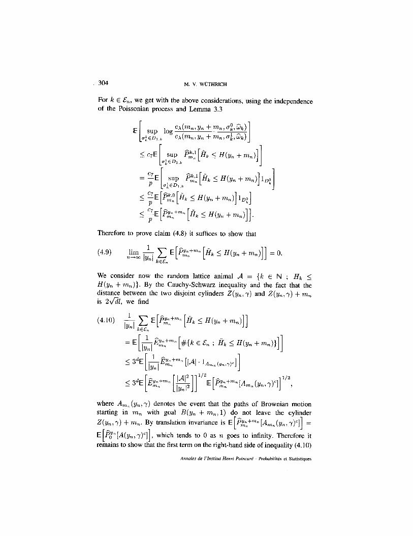
304 M. V. WirTHRICH

For k E En, we get with the above considerations, using the independence Y

of the Poissonian process and Lemma 3.3

Therefore to prove claim (4.8) it suffices to show that

We consider now the random lattice animal A = {k E N ; Hk 5

H(y, + m,)}. By the Cauchy-Schwarz inequality and the fact that the distance between the two disjoint cylinders Z(y,, y) and Z(y,, 7) + m, is 2&l, we find

where A m,(yn, y) denotes the event that the paths of Brownian motion starting in m, with goal B(yy, + m,, 1) do not leave the cylinder

z(h 7) + m,. By translation invariance is E [ p$=n+mn I A

E pin Myn, Y)“l] 1 dYm] =

which tends to 0 as n goes to infinity. Therefore it remains to show that the first term on the right-hand side of inequality (4.10)

Ann&s de l’fnstirut Henri Poincare! - F’robabilitks et Statistiques


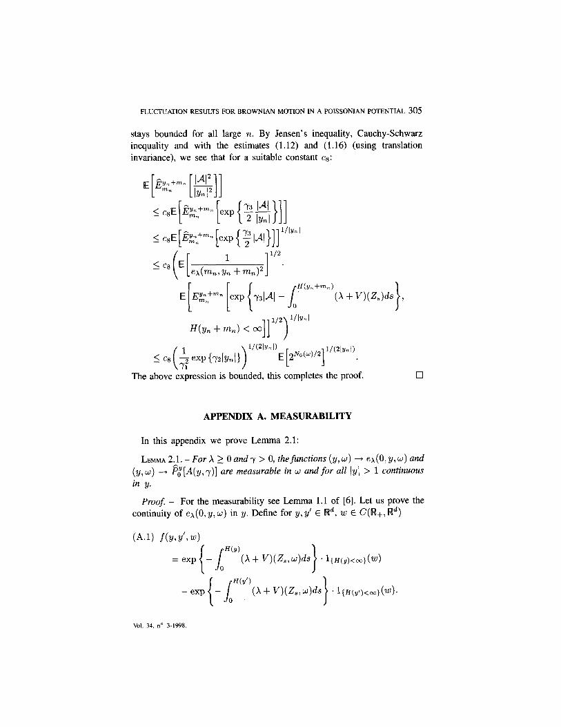
stays bounded for all large 72. By Jensen’s inequality, Cauchy-Schwarz inequality and with the estimates (1.12) and (1.16) (using translation invariance), we see that for a suitable constant cs:

The above expression is bounded, this completes the proof. q

APPENDIX A. MEASURABILITY

In this appendix we prove Lemma 2.1:

LEMMA 2.1. - For X 2 0 and y > 0, thefunctions (y, W) + ex(O, y, w) and

(Y, w) --+ %[~YJ)I are measurable in w and for all (y\ > 1 continuous in y.

Proof. - For the measurability see Lemma 1.1 of [6]. Let us prove the continuity of ex(O, y, w) in y. Define for y, y’ E I@, w E C(W+, l@)

(A-1) f(y, Y’, w) H(Y)

CA + v>(zs, w)ds * l{H(y)<m}(W)

CA + V)(-%w)ds

I

’ 1{H(y’)<co}(W)-

Vol. 34, no 3-1998.

306 M. V. WtiTHRICH

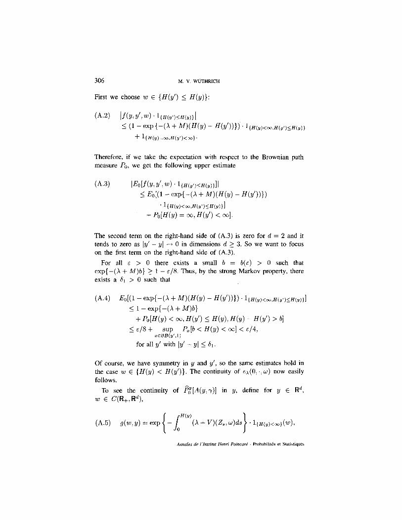
First we choose w E {H(y’) 5 H(y)}:

(A.21 If(y> Y’, w) . ~IHW)<H(~)~ 1 I (1 - exp 1-V + W(fW - fW))H * ~w(~)<~,H(~~)~H(~)I

+ lIff(y)= rn,ff(Y’)<oo)~

Therefore, if we take the expectation with respect to the Brownian path measure PO, we get the following upper estimate

(A.31 PoV(Y1 Y’T w> . 1{H(Y’)lH(Y)Ill I E0[(1- exp{-(X + W(W) - WY’NH

. l{H(Y)<~,H(Y’)lH(Y)}l + Pop(Y) = 037 H(Y’) < ml.

The second term on the right-hand side of (A.3) is zero for d = 2 and it tends to zero as ] y’ - y ] --t 0 in dimensions d > 3. So we want to focus on the first term on the right-hand side of (A.3).

For all E > 0 there exists a small b = b(e) > 0 such that exp{-(X + &I)b} > 1 - E/S Thus, by the strong Markov property, there exists a 61 > 0 such that

(A.41 Eo[(~ - exp{--(A + M)(H(Y) - H(Y’)))). ~~H(~)<~,H(~~I(~)I

5 1 - exp{-(X + A4)b)

+ Pop-f(Y) < =J, NY’) 5 H(Y), H(Y) - WY’) > bl I E/8 + sup Pz[b < H(y) < co] < E/4,

z@B(y’,l)

for all y’ with ]y’ - y] I 61.

Of course, we have symmetry in y and y’, so the same estimates hold in the case w E {H(y) < H(y’)}. The continuity of ex(O, .,w) now easily follows.

To see the continuity of @[A(y, y)] in y, define for y E Wd, w E C(W+Jq,

(A.5) g(w, y) = exp - lHCyi(A + V)(zs, w)ds * l{H(y)<m)(WL

Ann&s de l’lnstitut ffenri PoincarP - Probabilitt?s et Statistiques


and

(A.6) h(w> Y> = lA(y,r) ’ l{H(y)<oo}(W).

Using the continuity of ex(O, ., w) and the tubular estimate (1.12), we see that it suffices to show that Ea[g(w, .)h(w, e)] is continuous. For y, y’ E Wd, w E a, we have, using the triangle inequality,

(A.71 lEo[g(w, Y)h(W, Y)] - EOiSh~ Y’Y44 Y’)ll I (EO[(S(W? Y> - dw, Y’)MW~ Y)lI + p3o[s(w, Y’)(VW: Y> - VW, Y’Nl.

The first term on the right-hand side of (A.7) tends to zero as ]y - y’] -+ 0, using the same observations as done in the proof of the continuity of ex(O, y, w). So we want to focus on the second term on the right-hand side of (A.7). First we choose w E {H(y’) < H(y)}, then we have

(A-8) IEOMW Y’)(cG Y> - ww, Y’N * 1{Hw)<Hdl I EoW(w Y> - VW, ~‘11 . 1w,~)<~wocjl

+ Po[H(Y’) < 00, H(Y) = 4.

For the second term on the right-hand side of (A.8) we use the same remark as after (A.3), whereas for the first term we see, using the strong Markov property, that it tends to zero as (y - y’] -+ 0. This finishes the proof of the lemma. 0

ACKNOWLEDGEMENT

Let me thank Professor A. S. Sznitman for giving me very helpful suggestions.

REFERENCES

[l] M. AIZENMAN and J. WEHR, Rounding effects of first order phase transition. Commun. Math. Phys., Vol. 130, 1990, pp. 489-528.

[2] H. KESTEN, Aspects of first-passage percolation. In Ecole d’&t! de Probabilitks de St. Flour, Leer. Notes in Math., Vol. 1180. Springer-Verlag, 1985, pp. 125-264.

[3] H. KESTEN, On the speed of convergence in first-passage percolation. Ann. Appl. Prob., Vol. 3, 1993, pp. 296-338.

[4] C. LICEA, C. M. NEWMAN and M. S. T. PIZA, Superdiffusivity in first-passage percolation. Prob. Theory Ret. Fieids, Vol. 106, 1996, pp. 559-591.

Vol. 34. no 3-1998

308 M. V. WijTHRICH

[5] C. M. NEWMAN and M. S. T. F’IZA, Divergence of shape fluctuations in two dimensions. Ann. Prob., Vol. 23, 1995, pp. 977-1005.

[6] A. S. SZNITMAN, Shape theorem, Lyapounov exponents and large deviations for Brownian motion in a Poissonian potential. Comm. Pure Appl. Math., Vol. 47, 12, 1994, pp. 1655-1688.

[7] A. S. SZNITMAN, Crossing velocities and random lattice animals. Ann. Prob., Vol. 23, 1995, pp. 1006-1023.

[8] A. S. SZNITMAN, Distance fluctuations and Lyapounov exponents. Ann. Prob., Vol. 24, 1996, pp. 1507-1530.

[9] J. WEHR and M. AIZENMAN, Fluctuations of extensive functions of quenched random couplings. J. Stat. Phys., Vol. 60, 1990, pp. 287-306.

[lo] M. V. WUTHRICH, Superdiffusive behaviour of two dimensional Brownian motion in a Poissonian potential. To appear in The Annuls of Probability.

(Manuscript received on December 9, 1996: Revised on November 7, 1997.)

Ann&s de l’lnsritur Henn’ PoincarP - F’robabilitks et Statistiques

Documents

Fluctuation results for Brownian motion in a Poissonian potential