Embed Size (px)
Citation preview
Brazilian banded iron formations: a geological and geotechnical
characterisation from hard and fresh to weak and completely
weathered rocks
TEÓFILO AQUINO VIEIRA DA COSTA
This thesis is presented for the degree of
Doctor of Philosophy
The University of Western Australia
School of Civil, Environmental and Mining Engineering
June 2021

ii
iii
THESIS DECLARATION
I, Teófilo Aquino Vieira da Costa, certify that:
This thesis has been substantially accomplished during enrolment in the degree.
This thesis does not contain material which has been submitted for the award of any other
degree or diploma in my name, in any university or other tertiary institution.
No part of this work will, in the future, be used in a submission in my name, for any other degree
or diploma in any university or other tertiary institution without the prior approval of The
University of Western Australia and where applicable, any partner institution responsible for the
joint award of this degree.
This thesis does not contain any material previously published or written by another person,
except where due reference has been made in the text and, where relevant, in the Declaration
that follows.
The works are not in any way a violation or infringement of any copyright, trademark, patent, or
other rights whatsoever of any person.
The research involving geotechnical data reported in this thesis was assessed and approved by
The University of Western Australia and Vale S.A.
The work described in this thesis was funded by Vale S.A.
Technical assistance was kindly provided by the Australian Centre for Geomechanics (ACG),
E-precision Laboratory, Geocontrole Br. Sondagens S.A. and the Petrophysics laboratory of
Federal University of Campina Grande for laboratorial experiments that is analysed in this thesis.
This thesis contains published work and work prepared for publication, all of which has been
co-authored.
Date: June 21, 2021
iv
PUBLICATIONS ARISING FROM THIS THESIS
Conference papers – already published:
Costa, TAV, Dight, PM, Mercer, K & Marques, EAG 2015, ‘An overview of the weathering process
and preliminary density and UCS correlations for fresh itabirites in Vale mines on the western
side of the Iron Quadrangle, Brazil’, Proceedings of the Iron Ore Conference, Australasian
Institute of Mining and Metallurgy, Perth, Australia.
Costa, TAV, Mercer, K, Dight, PM & Marques, EAG 2015, ‘Weathered banded iron formations in
Vale iron ore mines on the western side of the Iron Quadrangle, Brazil: weak hematitite and
weathered argillaceous itabirite geotechnical characteristics and implications of matric suction
effects on slope stability’, Proceedings of the 25th International Symposium on Slope Stability in
Open Pit Mining and Civil Engineering, Australian Centre for Geomechanics, Perth, Australia.
Prepared as manuscript – not published:
Intact rock strength characteristics and elastic static properties of fresh Brazilian banded iron
formations.
Petrophysical characteristics and elastic dynamic properties of fresh to moderately weathered
Brazilian banded iron formations.
Weak rock behaviour of highly to completely weathered Brazilian banded iron formations.
Weathering profile, intact rock strength and elastic characteristics of Brazilian banded iron
formations.
v
STATEMENT OF CANDIDATE CONTRIBUTION (%)
This thesis contains co-authored published and unpublished papers. The percentage of the work
of co-authors is presented below.
Costa, TAV (70%), Dight, PM (20%), Mercer, K (5%) & Marques, EAG (5%) 2015, ‘An overview of
the weathering process and preliminary density and UCS correlations for fresh itabirites in Vale
mines on the western side of the Iron Quadrangle, Brazil’, Proceedings of the Iron Ore
Conference, Australasian Institute of Mining and Metallurgy, Melbourne, Australia.
Costa, TAV (70%), Mercer, K (20%), Dight, PM (5%) & Marques, EAG (5%) 2015, ‘Weathered
banded iron formations in Vale iron ore mines on the western side of the Iron Quadrangle, Brazil:
weak hematitite and weathered argillaceous itabirite geotechnical characteristics and
implications of matric suction effects on slope stability’, Proceedings of the 25th International
Symposium on Slope Stability in Open Pit Mining and Civil Engineering, Australian Centre for
Geomechanics, Perth, Australia.
Costa, TAV (80%), Dight, PM (10%) and Marques, EAG (10%) Intact rock strength characteristics
and elastic static properties of fresh Brazilian banded iron formations – Brazil. Not published.
Costa, TAV (80%), Marques, EAG (10%), Dight, PM, (5%) and Lima, P (5%) Petrophysical
characteristics and elastic dynamic properties of fresh to moderately weathered Brazilian
banded iron formations. Not published.
Costa, TAV (80%), Dight, PM (10%) and Marques, EAG (10%) Weak rock behaviour of highly to
completely weathered Brazilian banded iron formations. Not published.
Costa, TAV (80%), Mercer, K (10%), Dight, PM (5%) and Marques, EAG (5%) Weathering profile,
intact rock strength and elastic characteristics of Brazilian banded iron formations. Not
published.

vi
vii
ABSTRACT
Brazilian Proterozoic banded iron formations (BIF), classified as low-grade ore, ‘itabirites’ are
divided into quartzitic, dolomitic and amphibolitic and high-grade ore ‘hematitite’, together are
the main iron host rock of the Iron Quadrangle mines in Brazil. Their genesis is controversial, but
it is agreed that metamorphic and tectonic events as well as the supergene and hypogene
enrichment are responsible for reconcentrating the iron, and weathering processes are
responsible for reducing the original high intact rock strength, generating deep and
heterogeneous weathered profiles with low strength rocks (weak rocks) reaching 400 m depth.
Based on field investigation and laboratory tests, from 15 different mines, this thesis aims to
determine intact rock strength parameters and petrophysical proprieties (macro and micro
scales) in different weathering profile levels (horizons and zones), highlighting geological and
geotechnical characteristics considering the degree of anisotropy defined by the compositional
metamorphic banding (heterogeneity). Establishing relationships between petrophysical, rock
strength and elastic parameters, proposing empirical correlation equations.
To reach the thesis goals, rock laboratory tests (triaxial, unconfined compressive strength – UCS,
P and S wave and Brazilian test) and soil laboratory tests (Atterberg limits, particle size
distribution and soil-water characteristic curves, saturated and unsaturated direct shear test,
triaxial – CIU and permeability test) were undertaken for each typology in different anisotropy
directions. Additionally, petrographic thin sections, geological and geotechnical field
investigation, and permeability in situ tests were assessed.
All test results and Vale’s internal database were assembled and evaluated, and a complete
failure envelope for each typology, was determined to describe the intact rock and shear strength
parameters variance in association with the geological and geotechnical characteristics along
the weathering profile. For each weathering level it was concluded that:
For fresh typologies, the anisotropy ratio and index, respectively based in the UCS tests and Vp
measures, are low to isotropic unless for fresh dolomitic itabirites that present a fairly to
moderately anisotropy ratio. Even with a moderate UCS results dispersion, there is a direct
correlation between iron content, bulk density and UCS parameters for hematitite and itabirites,
and inverse correlation with total porosity. For these types, the main characteristics responsible
for defining the rock strength and anisotropy are the mineralogy and the rock fabric. On this
matter, hard hematitite is the stronger strength typology followed by fresh quartzitic,
amphibolitic and dolomitic itabirites. Hard hematitite also presents extremely high elastic
viii
parameters followed by amphibolitic and quartzitic itabirites and dolomitic itabirites presented
the lower elastic behaviour.
Also, for fresh rocks positioned at the bedrock of the BIF weathering horizon, empirical
correlations equations for UCS, Young´s Module, bulk density and P and S wave velocity were
established, which indicate a reliable, straightforward, and low-cost method which can be used
to predict, with acceptable accuracy, intact rock strength and elastic parameters.
Moderately weathered typologies, positioned at saprorock and saprolite horizons, even with a
small number of tests, showed fairly to moderately anisotropy index due to the higher total
porosity and lower bulk density, behaving like a soil when highly weathered (saprolite horizon),
or rock when moderately weathered (saprorock horizon). For these types, the heterogeneity is
defined mainly by the total porosity, however the mineral compositing plays an important role.
The completely weathered rocks are characterised as saprolite or in situ residual soil horizons.
For these BIF rock-like soil types, the bulk density, particle size distribution, permeability, total
porosity, and water content are the most important parameters for typology shear strength
variation. The low anisotropic ratio generally obtained affect minimally the low shear strength
values of weathered BIF types. The weathered argillaceous itabirite presents the lowest
permeability and highest clay content that induces a matric suction effect (up to 80 kPa) and as
an aquiclude can keep the negative porewater pressure (suction) describing an important
unsaturated behaviour.
This thesis concludes that for BIF rocks each weathering horizon and level presents a typical
intact rock strength, elastic parameters, and intrinsic petrophysical proprieties defining a specific
geomechanical behaviour mainly controlled by the binomials iron content/bulk density, total
porosity/permeability, and the mineral composition/bands thickness. Ultimately, the weathering
profile horizon and level control slope stability and failure mechanisms not only for long-term
excavations but also for temporary slopes from shallow to deep iron ore mines.
ix
TABLE OF CONTENTS
THESIS DECLARATION ........................................................................................................... III
ABSTRACT ........................................................................................................................... VII
LIST OF TABLES ................................................................................................................ ..XXV
LIST OF GRAPHS ............................................................................................................. . XXVII
LIST OF SYMBOLS ............................................................................................................. XXIX
ACKNOWLEDGEMENTS .................................................................................................... .XXXI
DEDICATION ................................................................................................................... . XXXII
AUTHORSHIP DECLARATION: CO-AUTHORED PUBLICATIONS .......................................... XXXIII
CHAPTER 1. INTRODUCTION ............................................................................................... 1
1.1 Problem statement ....................................................................................................... 1
1.2 Research objectives ....................................................................................................... 3
1.3 Research limitation ....................................................................................................... 5
1.4 Thesis contributions ...................................................................................................... 7
1.5 Thesis organisation ........................................................................................................ 8
CHAPTER 2. LITERATURE REVIEW ..................................................................................... 11
2.1 Regional geological settings ........................................................................................ 11
2.2 BIF geological settings ................................................................................................. 12
2.2.1 Itabirites and hematitites geotechnical and geological settings ......................... 13
2.3 Weathering profile settings ......................................................................................... 18
2.3.1 Failure criteria evaluation for the BIF’s weathering profiles ............................... 21
2.3.2 BIF weathering profile determination and implications for slope stability ........ 23
2.4 Rock mechanics approaches for fresh to moderately weathered BIF ........................ 25
2.5 Soil mechanics approaches for completely weathered BIF ........................................ 27
CHAPTER 3. METHODOLOGY ............................................................................................ 33
3.1 Fieldwork and sampling .............................................................................................. 34
3.2 Database consistency approachs and definitions ....................................................... 34
3.3 Laboratory tests .......................................................................................................... 38
3.3.1 Sampling validation and laboratory test grouping .............................................. 38
3.3.2 Rock mechanics tests .......................................................................................... 40
3.3.3 Soil mechanics tests ............................................................................................ 44
3.3.4 Petrographic thin sections .................................................................................. 48
3.4 Software used.............................................................................................................. 49
CHAPTER 4. INTACT ROCK STRENGTH CHARACTERISTICS AND ELASTIC STATIC PROPERTIES OF FRESH BRAZILIAN BANDED IRON FORMATIONS .............................................................. 51
x
ABSTRACT ........................................................................................................................... 51
4.1 Introduction................................................................................................................. 52
4.2 Objectives and approaches ......................................................................................... 53
4.3 Geological and geotechnical settings .......................................................................... 55
4.3.1 Regional geological settings ................................................................................ 55
4.3.2 BIF geological and geotechnical settings ............................................................. 57
4.3.3 Intact rock strength parameters, anisotropy and petrophysical properties correlations ......................................................................................................................... 62
4.4 Methodology ............................................................................................................... 68
4.4.1 Laboratory tests .................................................................................................. 73
4.5 Results ......................................................................................................................... 76
4.5.1 Mineralogical and fabric overview ...................................................................... 76
4.5.2 BIF, heterogeneity and anisotropy ...................................................................... 80
4.5.3 Intact rock strength anisotropy ........................................................................... 83
4.5.4 BIF characterisation of geomechanical properties and parameters ................... 88
4.6 Discussion .................................................................................................................. 100
4.6.1 BIF compositional metamorphic banding heterogeneity and strength anisotropy ........................................................................................................................... 100
4.6.2 Petrophysical, geological and geomechanical properties characterisation and correlations ....................................................................................................................... 103
4.7 Conclusion ................................................................................................................. 108
CHAPTER 5. PETROPHYSICAL CHARACTERISTICS AND ELASTIC DYNAMIC PROPERTIES OF FRESH TO MODERATELY WEATHERED BRAZILIAN BANDED IRON FORMATIONS ................. 113
ABSTRACT ......................................................................................................................... 113
5.1 Introduction............................................................................................................... 114
5.2 Objectives and approaches ....................................................................................... 116
5.3 Geological and geotechnical settings ........................................................................ 117
5.3.1 Regional geological settings .............................................................................. 117
5.3.2 BIF geological and geotechnical settings ........................................................... 119
5.3.3 P and S wave velocities, dynamic elastic and petrophysical properties correlations ........................................................................................................................... 126
5.4 Methodology ............................................................................................................. 133
5.4.1 Laboratory tests ................................................................................................ 136
5.5 Results ....................................................................................................................... 140
5.5.1 Mineralogical and fabric overview .................................................................... 140
5.5.2 Heterogeneity and anisotropy evaluations ....................................................... 146
xi
5.5.3 Anisotropy evaluations of dynamic elastic parameters and petrophysical properties .......................................................................................................................... 151
5.5.4 Isotropic evaluations of dynamic elastic parameters and petrophysical properties ........................................................................................................................... 159
5.6 Discussion .................................................................................................................. 175
5.6.1 BIF compositional metamorphic banding heterogeneity and the anisotropy behaviour .......................................................................................................................... 175
5.6.2 Correlations between wave velocity propagation, dynamic elastic, and petrophysical proprieties .................................................................................................. 178
5.6.3 Comparing dynamic with static parameters .................................................... 181
5.7 Conclusion ................................................................................................................. 181
CHAPTER 6. WEAK ROCK BEHAVIOUR OF HIGHLY TO COMPLETELY WEATHERED BANDED IRON FORMATIONS FROM IRON QUADRANGLE – BRAZIL .................................................. 185
ABSTRACT ......................................................................................................................... 185
6.1 Introduction............................................................................................................... 187
6.2 Objectives and approaches ....................................................................................... 189
6.3 Geological and Geotechnical settings ....................................................................... 190
6.3.1 Regional geological setting ................................................................................ 190
6.3.2 Banded iron formation geological settings ....................................................... 191
6.3.3 Banded iron formations weathering profile ..................................................... 199
6.4 Saturated and unsaturated approaches brief literature review ............................... 202
6.4.1 Industry overview .............................................................................................. 202
6.4.2 Application of unsaturated theory to open pit mining ..................................... 205
6.4.3 Soil–water characteristic curves ....................................................................... 210
6.5 Methodology ............................................................................................................. 212
6.5.1 Overview ........................................................................................................... 212
6.5.2 Laboratory tests ................................................................................................ 216
6.6 Results ....................................................................................................................... 222
6.6.1 Fabric and mineralogical thin section overview ................................................ 222
6.6.2 Unified soil classification system ....................................................................... 228
6.6.3 Bulk density ....................................................................................................... 234
6.6.4 Coefficient of permeability ................................................................................ 234
6.6.6 Saturated shear strength characteristics .......................................................... 239
6.6.7 Unsaturated shear strength characteristics ...................................................... 252
6.7 Discussion .................................................................................................................. 256
6.8 Conclusion ................................................................................................................. 261
xii
CHAPTER 7. WEATHERING PROFILE, INTACT ROCK STRENGTH AND ELASTIC CHARACTERISTICS OF BRAZILIAN BANDED IRON FORMATIONS ......................................... 265
ABSTRACT ......................................................................................................................... 265
7.1 Introduction............................................................................................................... 267
7.2 Objectives and approaches ....................................................................................... 268
7.3 Geological and geotechnical settings ........................................................................ 269
7.3.1 Regional geological settings .............................................................................. 269
7.3.2 BIF geological and geotechnical settings ........................................................... 271
7.3.3 Banded iron formation weathering profiles ..................................................... 284
7.3.4 Failure criteria evaluation for the BIF’s weathering profiles ............................. 286
7.4 Methodology ............................................................................................................. 288
7.4.1 Laboratory tests ................................................................................................ 293
7.5 Results ....................................................................................................................... 297
7.5.1 Banded iron formation weathering profiles ..................................................... 297
7.5.2 BIF mineralogical and fabric overview .............................................................. 302
7.5.3 Heterogeneity and anisotropy for BIF weathering profiles, a micro overview . 308
7.5.4 Evaluation of the BIF anisotropy throughout the complete weathering profile .... ........................................................................................................................... 312
7.5.5 BIF isotropic approach throughout the complete weathering profile .............. 322
7.5.6 Strength envelope of best fit curve for completely weathered BIF profile ...... 328
7.6 Discussion .................................................................................................................. 340
7.7 Conclusion ................................................................................................................. 346
CHAPTER 8. CONCLUDING REMARKS .............................................................................. 351
8.1 Fresh to moderately weathered BIF geological and geomechanical characterisation ................................................................................................................................... 351
8.2 Completely weathered to residual soils and weak BIF geological and geomechanical characterisation .................................................................................................................... 356
8.3 BIF completely weathered profile geological and geomechanical characterisation 359
CHAPTER 9. RECOMMENDATIONS FOR FUTURE WORK .................................................. 365
9.1 BIF hard rock behaviour ............................................................................................ 365
9.2 BIF weak rock behaviour ........................................................................................... 366
9.3 Future approaches for thesis limitations .................................................................. 366
REFERENCES ...................................................................................................................... 367
APPENDIX I ........................................................................................................................ 387
APPENDIX II ....................................................................................................................... 419
APPENDIX III ...................................................................................................................... 447
APPENDIX IV ...................................................................................................................... 451
xiii
APPENDIX V ....................................................................................................................... 469
APPENDIX VI ...................................................................................................................... 475
APPENDIX VII ..................................................................................................................... 481
APPENDIX VIII .................................................................................................................... 487

xiv
xv
LIST OF FIGURES
FIGURE 1.1 RESEARCH AIMS INTERCONNECTION .............................................................................. 5
FIGURE 1.2 STUDIED MINES LOCALISATION, STRATIGRAPHIC COLUMN, AND IRON QUADRANGLE GEOLOGICAL
SETTINGS (MODIFIED FROM MORGAN ET AL. 2013) ......................................................................... 7
FIGURE 2.1 SUMMARY FOR ALL STUDIED BIF TYPES, SHOWING IN THE GREEN DOTTED SQUARE THE HIGH UCS
VALUES, IN BLUE THE INTERMEDIATE, AND RED THE LOW UCS VALUES (AFTER MARTIN & STACEY 2018) 18
FIGURE 2.2 SCHEMATIC DIAGRAM OF TYPICAL TROPICAL RESIDUAL SOIL PROFILE PRESENTING THE HORIZONS
ON THE LEFT SIDE AND ZONES ON THE RIGHT SIDE (MODIFIED FROM DEERE & PATTON 1971) ............... 19
FIGURE 2.3 THE THREE REGIONS FOR THE HOEK–BROWN STRENGTH CURVE AND THE EQUIVALENT MOHR–
COULOMB STRENGTH LINE (LIN ET AL. 2014) ................................................................................ 22
FIGURE 2.4 MOHR–COULOMB FAILURE ENVELOPE FOR A SATURATED SOIL ........................................ 28
FIGURE 2.5 EXTENDED MOHR–COULOMB FAILURE ENVELOPE FOR UNSATURATED SOILS (GAN & FREDLUND
ET AL. 1988) ........................................................................................................................... 30
FIGURE 3.1 CLASSIFICATION BASED ON ANISOTROPIC RATIO, SINGH ET AL. (1989) AND ΒANGLE DEFINITION
AFTER MCLAMORE & GRAY (1967) ............................................................................................ 37
FIGURE 3.2 P WAVE VELOCITY ANISOTROPIC INDEX, MODIFIED FROM PERUCHO ET AL. (2014) ..................
............................................................................................................................. 38
FIGURE 3.3 WEATHERING GRADE AND ESTIMATION OF THE ROCK STRENGTH TABLE PLOTTED FOR THE
THREE MAIN GROUPS. THE APPLIED LABORATORY TESTS FOR EACH STRENGTH LEVEL ARE GROUPED BY THE
GREEN DOTTED SQUARE FOR HARD ROCKS, A BLUE DOTTED SQUARE FOR MODERATE ROCK STRENGTH AND
THE RED DOTTED SQUARE FOR WEAK ROCK AND SOIL-LIKE MATERIAL STRENGTH (AFTER MARTIN & STACEY
2018) ......................................................................................................................... 39
FIGURE 3.4 THE MECHANICAL AND ELECTRONIC APPARATUS (AUTOLAB-500®) USED FOR P AND S WAVE
VELOCITIES AND EFFECTIVE POROSITY TESTS (LIMA & COSTA 2016) .................................................. 44
FIGURE 3.5 THE SCHEMATIC MODIFIED SUCTION CONTROLLED DIRECT SHEAR TEST APPARATUS FOR
TESTING THE SHEAR STRENGTH OF UNSATURATED SOILS, FROM GAN ET AL. (1988) ............................. 48
FIGURE 4.1 MINE LOCATIONS (RED CIRCLES) AND IRON QUADRANGLE GEOLOGICAL SETTINGS (MODIFIED
FROM MORGAN ET AL. 2013) .................................................................................................... 55
FIGURE 4.2 A (LEFT), HHE AT MICROSCOPE VIEW WITH GRANULAR CRYSTALS OF HEMATITE (LIGHT GREY)
AND SMALLER CRYSTALS OF HEMATITE MICROPLATES (LIGHT GREY) (HORTA & COSTA 2016). B (RIGHT),
OUTCROP OF FRACTURED HHE AT CAPITÃO DO MATO MINE ........................................................... 59
FIGURE 4.3 A (LEFT), SHOWS MICROPHOTOGRAPHY OF FQI PRESENTING TYPICAL QUARTZ BANDING
(WRITE CRYSTALS), GRANULAR TO TABULAR HEMATITE (LIGHT GREY) AND POROUS (BLACK) (HORTA & COSTA
2016). B (RIGHT), TYPICAL OUTCROP PRESENTING FRACTURES IN TAMANDUÁ MINE ........................... 60
xvi
FIGURE 4.4 A (LEFT), SHOWS MICROPHOTOGRAPHY OF A FAI HIGHLIGHTING THE PRESENCE OF FIBROUS
GOETHITE AN AMPHIBOLITE ACICULAR OLD CRYSTAL (DARK FIBRE MINERALS) IMMERSE ON QUARTZ BANDS
(HORTA & COSTA 2016). B (RIGHT), SHOWS A TYPICAL SLOPE OF FOLDED AND FRACTURED FAI AT JANGADA
MINE ......................................................................................................................... 61
FIGURE 4.5 A (LEFT), SHOWS A MICROPHOTOGRAPHY OF FDI HIGHLIGHTING THE TYPICAL BANDING OF
IRON DOLOMITE AND QUARTZ (BLUE LIGHT COLOUR), AND FERROAN DOLOMITE AND TABULAR HEMATITE
BANDS (DARK GREY) (HORTA & COSTA 2016). B (RIGHT), TYPICAL HAND SAMPLE OF FOLDED FDI ......... 62
FIGURE 4.6 CLASSIFICATION BASED ON ANISOTROPIC RATIO, SINGH ET AL. (1989) AND ΒANGLE DEFINITION
AFTER MCLAMORE & GRAY (1967) ............................................................................................ 72
FIGURE 4.7 P WAVE VELOCITY ANISOTROPIC INDEX, MODIFIED FROM PERUCHO ET AL. (2014) .......... 72
FIGURE 4.8 A (LEFT), FQI BANDS OF HEMATITE (LIGHT GREY) WITH SMALLER CRYSTAL SIZE IN CONTACT
WITH BANDS OF LARGER CRYSTALS OF GRANULAR QUARTZ (COLOURED) AND A ROUGH CONTACT BETWEEN
(DASHED RED LINE) (HORTA & COSTA 2016). B (RIGHT), HHE CONTACT LESS ROUGH (DASHED RED LINE)
BETWEEN LARGER GRANULAR HEMATITE (DARK BAND) WITH SMALLER CRYSTALS OF TABULAR HEMATITE
(LIGHT BAND) (HORTA & COSTA 2016) ....................................................................................... 81
FIGURE 4.9 A (LEFT), TYPICAL SPECULARITE ORIENTATION CRYSTAL (HORTA & COSTA 2016). B (LEFT),
FDI BANDS OF ORIENTED GRANULAR IRON DOLOMITE WITH LARGE CRYSTALS (LIGHT BROWN) AND BANDS OF
TABULAR HEMATITE MIXED WITH IRON DOLOMITE AND QUARTZ (DARK BROWN) (HORTA & COSTA 2016) ..
......................................................................................................................... 82
FIGURE 4.10 A (LEFT), PORE BANDS IN MASSIVE HHE. B (RIGHT), FAI THIN SECTION WITH PORES ALONG
BANDING (TABULAR HEMATITE – LIGHT GREY, AND QUARTZ – WHITE) FILLED BY GOETHITE (LIGHT RED)
(HORTA & COSTA 2016) ........................................................................................................... 83
FIGURE 4.11 HETEROGENEITY VARIATION ACCORDING TO THE INCREASE OF IRON CONTENT FROM POOR BIF
(IRON RICH COUNTRY ROCKS) TO RICHEST BIF (HEMATITITE) .......................................................... 102
FIGURE 5.1 STUDIED MINES LOCALISATION AND IRON QUADRANGLE GEOLOGICAL SETTINGS (AFTER
BAARS & ROSIÈRE 1997) ........................................................................................................ 119
FIGURE 5.2 A (LEFT), HHE AT MICROSCOPE VIEW WITH GRANULAR CRYSTAL OF HEMATITE (LIGHT GREY)
AND SMALLER CRYSTAL OF HEMATITE MICRO PLATES (LIGHT GREY) (HORTA & COSTA 2016). B (RIGHT),
OUTCROP OF FRACTURED HHE AT CAPITÃO DO MATO MINE ......................................................... 122
FIGURE 5.3 A (LEFT), MICROPHOTOGRAPHY OF FQI PRESENTING TYPICAL QUARTZ BANDS (LARGE
COLOURED CRYSTAL), GRANULAR TO TABULAR HEMATITE BAND (LIGHT GREY) AND PORES (BLACK) (HORTA &
COSTA 2016). B (RIGHT), TYPICAL OUTCROP PRESENTING FRACTURES IN TAMANDUÁ MINE ................ 123
FIGURE 5.4 A (LEFT), PWQI MICROPHOTOGRAPHY HIGHLIGHTING PRESENCE OF GOETHITE CEMENTING A
FRACTURE (HORTA & COSTA 2016). B (RIGHT), AN OVERVIEW OF TYPICAL PWGI SLOPE AT TAMANDUÁ
MINE ....................................................................................................................... 124
xvii
FIGURE 5.5 A (LEFT), FAI MICROPHOTOGRAPHY HIGHLIGHTING FIBROUS GOETHITE AND AMPHIBOLITE
ACICULAR OLD CRYSTAL (DARK FIBRE MINERALS) IMMERSED IN QUARTZ BANDS (HORTA & COSTA 2016). B
(RIGHT) TYPICAL MINE SLOPE FOLDED AND FRACTURED FAI AT JANGADA MINE ................................. 125
FIGURE 5.6 A (LEFT), PWGI AT MICROSCOPE VIEW SHOWING IN RED ORANGE THE LARGE AMOUNT OF
GOETHITE (HORTA & COSTA 2016). B (RIGHT), TYPICAL PWGI FROM JANGADA MINE SLOPE ............. 125
FIGURE 5.7 A (LEFT), FDI MICROPHOTOGRAPHY HIGHLIGHTING TYPICAL BANDING OF DOLOMITE AND
QUARTZ (LIGHT COLOUR) INTERLAYERED BY BANDS OF HEMATITE AND QUARTZ (DARK COLOURS) (HORTA &
COSTA 2016). B (RIGHT), TYPICAL FOLDED FDI HAND SAMPLE ....................................................... 126
FIGURE 5.8 P WAVE VELOCITY ANISOTROPIC INDEX MODIFIED FROM SAROGLOU & TSIAMBAOS (2007),
AND ΒANGLE DEFINED AFTER MCLAMORE & GRAY (1962) ............................................................ 135
FIGURE 5.9 A (LEFT), PORO-PERMEAMETER PRESSURE GAUGES. B (CENTRE), PRESSURE TRANSDUCTORS.
C (RIGHT), COMPRESSION CHAMBER (LIMA & COSTA 2016) ......................................................... 138
FIGURE 5.10 THE MECHANICAL AND ELECTRONIC APPARATUS USED TO MEASURE P AND S WAVE VELOCITIES
(LIMA & COSTA 2016) ............................................................................................................ 139
FIGURE 5.11 A (LEFT), FQI MICROPHOTOGRAPHY SHOWING BANDS OF LARGER GRANULAR QUARTZ (LIGHT
BROWN CRYSTALS) IN CONTACT WITH MICROPLATES OF HEMATITE (SMALL GREY AND LIGHT GREY CRYSTALS).
B (RIGHT), HHE THIN SECTION SHOWING CONTACT BETWEEN LARGER GRANULAR HEMATITE CRYSTALS (DARK
BAND) WITH SMALLER TABULAR HEMATITE CRYSTALS (LIGHT BAND) ................................................ 147
FIGURE 5.12 A (LEFT), HHE THIN SECTION PRESENTING AN ORIENTATED SPECULARITE LARGE PLATELETS
(LIGHT GREY ELONGATED MINERALS) ORIENTATED ACCORDING TO THE BANDING. B (RIGHT), FDI THIN
SECTION SHOWING BANDS OF GRANULAR DOLOMITE (LIGHT BANDS) AND BANDS OF TABULAR HEMATITE
(BROWN) AND PORES IN CONTACT (BLACK) HORTA & COSTA (2016) .............................................. 148
FIGURE 5.13 A (LEFT), PORE BANDS IN MASSIVE HHE. B (CENTRE), FWQI MICROPHOTOGRAPHY SHOWING
POROSITY (DELIMITED IN RED LINES) BETWEEN QUARTZ (LIGHTLY COLOURED) AND HEMATITE (LIGHT GREY)
CONTACT. C (RIGHT) PWGI PRESENTING HEMATITE (WHITE) AND QUARTZ (GREY) BANDS WITH DIFFERENT
CRYSTAL SIZES AT CONTACT (DARK); HORTA & COSTA (2016)............................................................ 150
FIGURE 5.14 A (TOP LEFT), GRAPH SHOWS VP VALUES FOR EACH ΒANGLE. B (TOP RIGHT) SHOWS VS FOR EACH
ΒANGLE. C (LOWER LEFT), GRAPH SHOWS EDYN VALUES FOR EACH ΒANGLE. D (LOWER RIGHT) SHOWS ΝDYN FOR
EACH ΒANGLE. IN ALL FIGURES, THE DASHED LINE IS THE ANISOTROPIC CURVE, COLOURED TRIANGLES ARE THE
FDI VALUE RESULTS AND THE BLACK TRIANGLES REPRESENT Β0°, RED Β45° AND BLUE Β90° ..................... 154
FIGURE 5.15 A (TOP LEFT), GRAPH SHOWS VP VALUES FOR EACH ΒANGLE. B (TOP RIGHT) SHOWS VS FOR EACH
ΒANGLE. C (LOWER LEFT), GRAPH SHOWS EDYN VALUES FOR EACH ΒANGLE. D (LOWER RIGHT) SHOWS ΝDYN FOR
EACH ΒANGLE. IN ALL FIGURES, THE DASHED LINE IS THE ANISOTROPIC CURVE, COLOURED TOP-DOWN TRIANGLES
ARE THE FAI VALUE RESULTS AND THE BLACK TRIANGLES REPRESENT Β0°, RED Β45° AND BLUE Β90°.......... 155
xviii
FIGURE 5.16 A (TOP LEFT), GRAPH SHOWS VP VALUES FOR EACH ΒANGLE. B (TOP RIGHT) SHOWS VS FOR EACH
ΒANGLE. C (LOWER LEFT), GRAPH SHOWS EDYN VALUES FOR EACH ΒANGLE. D (LOWER RIGHT) SHOWS ΝDYN FOR
EACH ΒANGLE. IN ALL FIGURES, THE DASHED LINE IS THE ANISOTROPIC CURVE, COLOURED SQUARES ARE THE FQI
VALUE RESULTS AND BLACK SQUARES REPRESENT Β0°, RED Β45°AND BLUE Β90° .................................... 157
FIGURE 5.17 A (TOP LEFT), GRAPH SHOWS VP VALUES FOR EACH ΒANGLE. B (TOP RIGHT) SHOWS VS FOR EACH
ΒANGLE. C (LOWER LEFT), GRAPH SHOWS EDYN VALUES FOR EACH ΒANGLE. D (LOWER RIGHT) SHOWS ΝDYN FOR
EACH ΒANGLE. IN ALL FIGURES, THE DASHED LINE IS THE ANISOTROPIC CURVE, COLOURED CROSSES ARE THE
PWQI/PWGI VALUE RESULTS AND THE BLACK CROSSES REPRESENT Β0°, RED Β45° AND BLUE Β90° .......... 158
FIGURE 5.18 A (LEFT), SHOWS THE DISPERSION GRAPH FOR VP. B (RIGHT), SHOWS THE VS DISPERSION
GRAPH. FOR THESE GRAPHS, EACH COLOUR AND SYMBOL REPRESENT A SINGLE LITHOTYPE AS PRESENTED IN
THE LEGEND. DASHED LIGHT BLUE LINES ARE THE GROUP LIMITS AND DASHED DARK BLUE CIRCLES ARE
HIGHLIGHTED SAMPLES GROUPING ............................................................................................ 163
FIGURE 5.19 THE CORRELATION BETWEEN VS/VP (WAVE VELOCITY RATIO) FOR THE SET OF SAMPLES
ANALYSED. THE DASHED LINE IS THE LINEAR ADJUSTED CURVE WITH ITS EQUATION. POINT ’A’ SHOWS THE
LIMITS BETWEEN MODERATELY WEATHERED AND FRESH ITABIRITES AND POINT ‘B’ SHOWS THE LIMITS
BETWEEN FRESH ITABIRITES AND HHE. EACH COLOUR AND SYMBOL REPRESENT A SINGLE LITHOTYPE .... 164
FIGURE 5.20 A (TOP LEFT) AND C (LOWER LEFT) SHOW, RESPECTIVELY, THE GRAPHS VP WITH EDYN AND VP
WITH ΝDYN FOR ALL EVALUATED LITHOTYPES. B (TOP RIGHT) AND D (LOWER RIGHT) SHOW, RESPECTIVELY,
GRAPHS FOR VS WITH EDYN AND VS WITH ΝDYN FOR ALL OF THE LITHOTYPES EVALUATED. THE DASHED LINES
ARE THE CORRELATION LINES FOR FRESH ITABIRITE (RED) AND MODERATELY WEATHERED ITABIRITE (BLACK)
MATERIALS, AND THE LEGEND SHOWS THE COEFFICIENT OF DETERMINATION. EACH COLOUR AND SYMBOL
REPRESENT A SINGLE LITHOTYPE ................................................................................................. 165
FIGURE 5.21 THE DISTRIBUTION OF ΡB FOR THE SET OF SAMPLES ANALYSED. EACH COLOUR AND SYMBOL
REPRESENT A SINGLE LITHOTYPE AND THE DASHED LIGHT BLUE LINES REPRESENT THE GROUPING LIMITS . 167
FIGURE 5.22 A (LEFT), SHOWS THE CORRELATION BETWEEN ΡB AND VP. B (RIGHT), SHOWS THE
CORRELATION BETWEEN ΡB WITH VS FOR ALL TESTED SAMPLES. FOR THESE GRAPHS, EACH COLOUR AND
SYMBOL REPRESENT A SINGLE LITHOTYPE AS PRESENTED IN THE LEGEND. THE DASHED LIGHT BLUE LINES
REPRESENT THE GROUP LIMITS AND CIRCLES AND SQUARES ARE HIGHLIGHTED SAMPLE GROUPINGS ...... 168
FIGURE 5.23 A (LEFT), SHOWS THE GRAPH FOR ΡB AND EDYN FOR ALL TESTED SAMPLES. DIFFERENT MARKS
AND COLOURS REPRESENT DIFFERENT LITHOTYPES. B (RIGHT), SHOWS THE CORRELATION BETWEEN ΡB AND
ΝDYN FOR ALL THE SAMPLES TESTED. FOR THESE GRAPHS, EACH COLOUR AND SYMBOL REPRESENT A SINGLE
LITHOTYPE AS PRESENTED IN THE LEGEND. THE DASHED LIGHT BLUE LINES ARE THE GROUP LIMITS ........ 169
FIGURE 5.24 DISPERSION GRAPH OF TOTAL POROSITY. FOR THIS GRAPH, EACH COLOUR AND SYMBOL
REPRESENT A SINGLE LITHOTYPE AS PRESENTED IN THE LEGEND. THE DASHED LIGHT BLUE LINES ARE THE
GROUPING LIMITS (WEATHERING GRADES) .................................................................................. 170

xix
FIGURE 5.25 DISPERSION GRAPH SHOWING THE RELATIONSHIP BETWEEN BULK DENSITY AND TOTAL
POROSITY FOR ALL TESTED SAMPLES. FOR THIS GRAPH, EACH COLOUR AND SYMBOL REPRESENT A SINGLE
LITHOTYPE AS PRESENTED IN THE LEGEND. THE DASHED LIGHT BLUE LINES ARE THE GROUP LIMITS AND THE
DASHED COLOURED CIRCLES ARE HIGHLIGHTED SAMPLE GROUPINGS ................................................ 171
FIGURE 5.26 A (LEFT), SHOWS THE RELATIONSHIP BETWEEN TOTAL POROSITY AND VP. B (RIGHT), SHOWS
THE RELATIONSHIP BETWEEN Ø AND VS FOR ALL THE SAMPLES. FOR THESE GRAPHS, EACH COLOUR AND
SYMBOL REPRESENT A SINGLE LITHOTYPE AS PRESENTED IN THE LEGEND THE DASHED LIGHT BLUE LINES ARE
THE GROUP LIMITS AND THE DASHED BLACK LINE IS THE ADJUSTED CURVE ......................................... 172
FIGURE 5.27 A (LEFT), SHOWS THE RELATIONSHIP BETWEEN DYNAMIC YOUNG’S MODULUS AND TOTAL
POROSITY FOR ALL OF THE SAMPLES TESTED. B (RIGHT), SHOWS THE RELATIONSHIP BETWEEN DYNAMIC
POISSON’S RATIO AND Ø FOR ALL OF THE SAMPLES TESTED. FOR THESE GRAPHS, EACH COLOUR AND SYMBOL
REPRESENT A SINGLE LITHOTYPE AS PRESENTED IN THE LEGEND. THE DASHED LIGHT BLUE LINES ARE THE
GROUP LIMITS AND THE DASHED LINE IS THE ADJUSTED CURVE ........................................................ 173
FIGURE 6.1 MINE LOCATIONS AND IRON QUADRANGLE GEOLOGICAL SETTINGS (MODIFIED FROM
MORGAN ET AL 2013) ............................................................................................................ 190
FIGURE 6.2 A (LEFT), MICROPHOTOGRAPH OF WHE AT SLOPE SCALE SHOWING TYPICAL BANDING. B
(RIGHT), IS A MICROPHOTOGRAPH SHOWING MICRO-BANDING IN WHE, GRANULAR AND LARGER HEMATITE
CRYSTALS (LARGER, LIGHT GREY) AND MICRO-PLATES OF TABULAR HEMATITE (SMALLER, LIGHT GREY) (COSTA
2009) ....................................................................................................................... 193
FIGURE 6.3 A (LEFT), MICROPHOTOGRAPHY OF HEMATITE CRYSTAL, WITH PORES AND GRANULOBLASTIC
TEXTURE DEFINING THE BANDED SUBTYPE (COSTA 2009). B (CENTRE), ORIENTED MICRO-PLATES OF
HEMATITE, DEFINING THE FOLIATED SUBTYPE (COSTA 2009). C (RIGHT), CLAST TEXTURE DEFINING THE
BRECCIATED SUBTYPE (COSTA 2009) ......................................................................................... 195
FIGURE 6.4 A (LEFT), WAI AT SLOPE SCALE SHOWING LAYERS OF CLAY MINERALS. B (RIGHT),
MICROPHOTOGRAPHY SHOWING BRECCIATED TEXTURE OF WAI (HORTA & COSTA 2016) .................. 197
FIGURE 6.5 A (LEFT), PHOTOGRAPH OF WQI AT SLOPE SCALE SHOWING SUBVERTICAL BANDING
(AUTHOR’S PERSONAL ARCHIVE). B (RIGHT), MICROPHOTOGRAPHY SHOWING BANDING OF TABULAR
HEMATITE (LIGHT GREY) AND GRANULOBLASTIC CRYSTALS OF QUARTZ (DARK GREY) OF WQI (HORTA &
COSTA 2016) ....................................................................................................................... 198
FIGURE 6.6 A (LEFT), PHOTOGRAPHY OF WGI AT SLOPE SCALE SHOWING BANDING OF OCHREOUS
GOETHITE, HEMATITE, AND QUARTZ. B (RIGHT), MICROPHOTOGRAPH SHOWING LAYERS OF GOETHITE,
QUARTZ AND GIBBSITE AND LAYERS OF HEMATITE AND GOETHITE OF WGI (HORTA & COSTA, 2016) ... 199
FIGURE 6.7 BILINEAR UNSATURATED MOHR–COULOMB ENVELOPE, MODIFIED FROM NEJAD &
MANAHILOH (2017)............................................................................................................... 207
xx
FIGURE 6.8 A (LEFT), SCHEMATIC MODIFIED SUCTION CONTROLLED DIRECT SHEAR TEST APPARATUS FOR
SHEAR STRENGTH OF UNSATURATED SOILS TESTING (GAN ET AL. 1988). B (RIGHT), EXTENDED MC FAILURE
ENVELOPE FOR UNSATURATED SOIL (GAN ET AL. 1988)................................................................. 208
FIGURE 6.9 DEFINITION OF SWCC VARIABLES (ZHAI & RAHARDJO 2012) ................................... 212
FIGURE 6.10 CLASSIFICATION BASED ON ANISOTROPIC RATIO, RAMAMURTHY ET AL. (1993) AND ΒANGLE
DEFINITION AFTER MCLAMORE & GRAY (1967) .......................................................................... 216
FIGURE 6.11 A (LEFT), LARGE CRYSTALS OF GRANULAR HEMATITE, SURROUNDED BY HEMATITE
MICRO-PLATES AND INTERCONNECTED POROSITY FILLED BY RESIN (WRITE) (HORTA &COSTA 2016). B
(RIGHT), GRANULAR AND HEMATITE MACRO-PLATES DEFINING A MODERATE VISUAL TOTAL POROSITY BAND
(HORTA &COSTA 2016) .......................................................................................................... 223
FIGURE 6.12 A (LEFT), MICROPHOTOGRAPHY OF MICRO-PLATES OF HEMATITE, MARTITE IN SUB-EUHEDRAL
LARGER CRYSTALS WITH THE PRESENCE OF OCHREOUS GOETHITE (BROWNISH) (HORTA &COSTA 2016). B
(RIGHT), BRECCIATED TEXTURE WITH LARGE PORES (BLACK) IN A FRAGMENT OF HEMATITE SURROUND BY
GOETHITE, MICRO-PLATES OF HEMATITE, GIBBSITE, AND A QUARTZ MATRIX (HORTA & COSTA 2016) ... 224
FIGURE 6.13 A (LEFT), OCHREOUS GOETHITE (RED), QUARTZ (YELLOW) AND GIBBSITE CEMENTING
CRYSTALS OF HEMATITE (BLACK) (HORTA &COSTA 2016). B (RIGHT), OCHREOUS GOETHITE AND GOETHITE
(RED AND ORANGE) CEMENTING THE MICRO-PLATES OF HEMATITE (HORTA & COSTA 2016) .............. 225
FIGURE 6.14 A (LEFT), BAND WITH GRANULAR HEMATITE (LARGE CREAM CRYSTALS), PORES (BLACK),
QUARTZ (LIGHT GREY) AND HEMATITE MICRO-PLATES (SMALL CREAM CRYSTALS) (HORTA & COSTA 2016). B
(RIGHT), MICRO-PLATES OF HEMATITE LAYER WITH PORE CONCENTRATION HIGHLIGHT AT WHITE DOTTED BOX
(HORTA & COSTA 2016) ......................................................................................................... 225
FIGURE 6.15 A (TOP), WAI PSD CURVES – GREEN. B (CENTRE), WHE PSD CURVES – RED. C (BOTTOM),
WQI AND WGI PSD CURVES – CYAN. BLACK CURVES ARE THE MEAN VALUE FOR EACH TYPE.................. 230
FIGURE 6.16 BOX PLOT GRAPH FOR BULK DENSITY RESULTS FROM PSD TESTS, PRESENTING FOR EACH
WEATHERED BIF TYPE THE MEAN LINE AND THE INCLUSIVE MEDIAN. DOTTED LINES REPRESENT THE LIMITS OF
EACH TYPE ................................................................................................................... 234
FIGURE 6.17 SHOWS THE SWCC ADJUSTED FITTING CURVES FOR ALL EVALUATED TYPOLOGIES AS
PROPOSED BY ZHAI & RAHARDJO (2012) ................................................................................... 236
FIGURE 6.18 A (LEFT), BEST FIT CURVE FOR VOLUMETRIC WATER CONTENT USED TO DETERMINE THE WAI
SAMPLE SWCC STATISTICAL MIDPOINT. B (RIGHT), BEST FIT CURVE FOR PERMEABILITY FUNCTION ........ 239
FIGURE 6.19 A (LEFT), WAI – NORMAL DISPLACEMENT VERSUS SHEAR DISPLACEMENT (BL-1). B (RIGHT),
WAI – EFFECTIVE SHEAR STRESS VERSUS SHEAR DISPLACEMENT. STAGE 1 = 100 KPA, STAGE 2 = 400 KPA
AND STAGE 3 = 800 KPA ......................................................................................................... 240
xxi
FIGURE 6.20 A (LEFT), WHE – NORMAL DISPLACEMENT VERSUS SHEAR DISPLACEMENT (BL-3). B
(RIGHT), WHE – EFFECTIVE SHEAR STRESS VERSUS SHEAR DISPLACEMENT. STAGE 1 = 100 KPA, STAGE 2 =
400 KPA AND STAGE 3 = 800 KPA ............................................................................................ 241
FIGURE 6.21 A (LEFT), WQI/WGI – NORMAL DISPLACEMENT VERSUS SHEAR DISPLACEMENT (BL-12).
B (RIGHT), WQI/WGI – EFFECTIVE SHEAR STRESS VERSUS SHEAR DISPLACEMENT. STAGE 1 = 100 KPA,
STAGE 2 = 400 KPA AND STAGE 3 = 800 KPA ............................................................................. 242
FIGURE 6.22 A (UPPER LEFT), CIU SHEAR STRESS VERSUS STRAIN CURVE FOR WAI AT Β0°. B (UPPER RIGHT),
EFFECTIVE POREWATER PRESSURE VERSUS AXIAL STRAIN FOR WAI AT Β0°. C (BOTTOM LEFT), CIU SHEAR
STRESS VERSUS STRAIN CURVE FOR WAI AT Β90°. D (BOTTOM RIGHT), EFFECTIVE POREWATER PRESSURE
VERSUS AXIAL STRAIN FOR WAI AT Β90°. SAMPLE – BL 1 – 10388 .................................................. 243
FIGURE 6.23 EFFECTIVE STRESS PATH CURVE (P-Q’) FOR 0° AND 90° WAI (SAMPLE – BL 1 – 10388)244
FIGURE 6.24 A (UPPER LEFT), CIU SHEAR STRESS VERSUS STRAIN CURVE FOR WHE AT Β0°. B (UPPER
RIGHT), EFFECTIVE POREWATER PRESSURE VERSUS AXIAL STRAIN FOR WHE AT Β0°. C (BOTTOM LEFT), CIU
SHEAR STRESS VERSUS STRAIN CURVE FOR WHE AT Β90°. D (LOWER RIGHT), EFFECTIVE POREWATER PRESSURE
VERSUS AXIAL STRAIN FOR WHE AT Β90°. SAMPLE – TAM BL-08 -10395 ....................................... 245
FIGURE 6.25 EFFECTIVE STRESS PATH (P-Q’) CURVE FOR 0° AND 90° WHE. SAMPLE – TAM BL-08 -10395
....................................................................................................................... 246
FIGURE 6.26 A (TOP LEFT), CIU SHEAR STRESS VERSUS STRAIN CURVE FOR WQI/WGI AT Β0°. B (TOP
RIGHT), EFFECTIVE POREWATER PRESSURE VERSUS AXIAL STRAIN FOR WQI/WGI AT Β0°. C (BOTTOM LEFT),
CIU SHEAR STRESS VERSUS STRAIN CURVE FOR WQI/WGI AT Β90°. D (BOTTOM RIGHT), EFFECTIVE
POREWATER PRESSURE VERSUS AXIAL STRAIN FOR WQI/WGI AT Β90°. SAMPLE – BL 12 – 10420 ....... 247
FIGURE 6.27 EFFECTIVE STRESS PATH (P-Q’) CURVE FOR 0° AND 90°WQI. SAMPLE – BL 12 – 10420 .....
....................................................................................................................... 248
FIGURE 6.28 A (LEFT), WAI LINEAR REGRESSION (BEST FIT) LINES IN Σ1 Σ3 STRESS SPACE FOR TOTAL
STRENGTH VALUES. B (RIGHT), LINEAR REGRESSION (BEST FIT) LINES IN Σ1Σ3 STRESS SPACE FOR EFFECTIVE
STRENGTH OBTAINED FROM ROCDATA 5.0 (ROCSCIENCE 2021) TRIAXIAL CIU TESTS CONSIDERING
DIFFERENT ANISOTROPY DIRECTIONS (45° – BLUE, 0° – RED, 90° – GREEN, AND ISOTROPIC – BLACK) ... 249
FIGURE 6.29 A (LEFT), WHE LINEAR REGRESSION (BEST FIT) LINES IN Σ1Σ3 STRESS SPACE FOR TOTAL
STRENGTH VALUES. B (RIGHT), LINEAR REGRESSION (BEST FIT) LINES IN Σ1Σ3 STRESS SPACE EFFECTIVE
PRINCIPAL STRESS OBTAINED FROM ROCDATA 5.0 (ROCSCIENCE 2021) TRIAXIAL CIU TESTS CONSIDERING
DIFFERENT ANISOTROPY DIRECTIONS (45° – BLUE, 0° – RED, 90° – GREEN, AND ISOTROPIC – BLACK) ... 250
FIGURE 6.30 A (LEFT), WQI/WGI LINEAR REGRESSION (BEST FIT) LINES IN Σ1 Σ3 STRESS SPACE FOR TOTAL
STRENGTH VALUES. B (RIGHT), LINEAR REGRESSION (BEST FIT) LINES IN Σ1Σ3 STRESS SPACE FOR EFFECTIVE
STRENGTH OBTAINED FROM ROCDATA 5.0 (ROCSCIENCE 2021) TRIAXIAL CIU TESTS CONSIDERING
DIFFERENT ANISOTROPY DIRECTIONS (45° – BLUE, 0° – RED, 90 – GREEN, AND ISOTROPIC – BLACK) .... 250
xxii
FIGURE 6.31 A (TOP LEFT), WAI NORMAL DISPLACEMENT VERSUS SHEAR DISPLACEMENT. B (BOTTOM
LEFT), SHEAR STRESS VERSUS SHEAR DISPLACEMENT. C (RIGHT), WATER DISCHARGE VERSUS SHEAR
DISPLACEMENT FOR SAMPLE BL_1 (Β0°), WITH MATRIC SUCTION LEVELS: STAGE 1 – 0 KPA, STAGE 2 – 20
KPA, STAGE 3 – 70 KPA AND STAGE 4 – 150KPA ........................................................................ 253
FIGURE 6.32 A (TOP LEFT), WHE NORMAL DISPLACEMENT VERSUS SHEAR DISPLACEMENT. B (BOTTOM
LEFT), SHEAR STRESS VERSUS SHEAR DISPLACEMENT. C (RIGHT), WATER DISCHARGE VERSUS SHEAR
DISPLACEMENT. SAMPLE BL_3 (Β0°). MATRIC SUCTION LEVELS: STAGE 1– 0 KPA, STAGE 2 – 20 KPA, STAGE
3 – 70 KPA AND STAGE 4 – 150KPA ......................................................................................... 254
FIGURE 6.33 A (TOP LEFT), WQI/WGI NORMAL DISPLACEMENT VERSUS SHEAR DISPLACEMENT.
B (BOTTOM LEFT), SHEAR STRESS VERSUS SHEAR DISPLACEMENT. C (RIGHT), WATER DISCHARGE VERSUS
SHEAR DISPLACEMENT. SAMPLE BL_12 (Β0°). MATRIC SUCTION LEVELS: STAGE 1 – 0 KPA, STAGE 2 – 20
KPA, STAGE 3 – 70 KPA AND STAGE 4 – 150 KPA ....................................................................... 254
FIGURE 7.1 MINE LOCATIONS AND IRON QUADRANGLE GEOLOGICAL SETTINGS (MODIFIED FROM
MORGAN ET AL. 2013) ........................................................................................................... 269
FIGURE 7.2 A (LEFT), HHE AT MICROSCOPE VIEW WITH GRANULAR CRYSTAL OF HEMATITE (LIGHT GREY –
B1) AND SMALLER CRYSTAL OF HEMATITE MICROPLATES (DARK GREY – B3) (HORTA & COSTA 2016). B
(RIGHT), OUTCROP OF FRACTURED HHE AT CAPITÃO DO MATO MINE ............................................. 274
FIGURE 7.3 MHE OUTCROP FOLDED IN A TAMANDUÁ PIT FACE SHOWING TYPICAL INTERLAYER BETWEEN
HHE AND WHE ..................................................................................................................... 274
FIGURE 7.4 A (LEFT), MICROPHOTOGRAPHY OF BRECCIATED WHE SHOWING GRANULAR LARGER
HEMATITES CRYSTALS (LIGHT GREY) AND CEMENT OF MICROPLATES OF HEMATITE (COSTA 2009). B (RIGHT),
WHE AT SLOPE SCALE SHOWING TYPICAL BANDING ...................................................................... 276
FIGURE 7.5 A (LEFT), MICROPHOTOGRAPH OF FDI SHOWING TYPICAL BANDING OF DOLOMITE AND
QUARTZ (LIGHT COLOUR), (HORTA & COSTA 2016); B (RIGHT), SHOWS TYPICAL HAND SAMPLE OF FRESH
FOLDED FDI ....................................................................................................................... 277
FIGURE 7.6 A (LEFT), WAI UNDER THE MICROSCOPE SHOWING BANDS OF MICROPLATES OF HEMATITE
AND SPECULARITE (LIGHT GREY) AND BANDS OF SMALLER CRYSTALS OF GIBBSITE AND OCHREOUS GOETHITE
(LIGHT BROWN) (HORTA & COSTA 2016). B (RIGHT), WAI IN AN EXPOSURE ................................... 278
FIGURE 7.7 A (LEFT), MICROPHOTOGRAPH OF FAI, ILLUSTRATING THE PRESENCE OF FIBROUS GOETHITE
AND ACICULAR AMPHIBOLE CRYSTALS (DARK FIBRE MINERALS) INCLUDED IN QUARTZ BANDS (HORTA & COSTA
2016); B (RIGHT), TYPICAL SLOPE OF FOLDED AND FRACTURED FAI (W2) IN JANGADA MINE .............. 279
FIGURE 7.8 TYPICAL PWGI SLOPE IN JANGADA MINE ............................................................... 280
FIGURE 7.9 A (LEFT), WGI UNDER THE MICROSCOPE SHOWING GOETHITE (ORANGE) AND ERODED
QUARTZ (YELLOW) (HORTA & COSTA 2016); B (RIGHT), A SLOPE AT TAMANDUÁ MINE SHOWING FOLDED
WGI INTERLAYERED WITH WHE ............................................................................................... 281
xxiii
FIGURE 7.10 A (LEFT), TYPICAL BANDING UNDER THE MICROSCOPE SHOWING HEMATITE BANDS (LIGHT
GREY) AND QUARTZ BANDS (RED), (HORTA & COSTA 2016); B (RIGHT), TYPICAL FQI SLOPE AT TAMANDUÁ
....................................................................................................................... 282
FIGURE 7.11 AN EXAMPLE OF LEACHING IN A TYPICAL PWGI SLOPE AT TAMANDUÁ MINE ................ 283
FIGURE 7.12 A (LEFT), WQI UNDER THE MICROSCOPE, SHOWING QUARTZ (GREY) AND MICROPLATES OF
HEMATITE (LIGHT GREY) (HORTA & COSTA 2016); B (RIGHT), WQI SLOPE DETAIL AT TAMANDUÁ MINE ....
................................................................................................................... 284
FIGURE 7.13 THE THREE REGIONS FOR THE HOEK–BROWN STRENGTH CURVE AND THE EQUIVALENT
MOHR–COULOMB STRENGTH LINE (LIN ET AL. 2014) ................................................................... 288
FIGURE 7.14 WEATHERING GRADE AND ESTIMATION OF THE ROCK STRENGTH TABLE PLOTTED FOR THE THREE
MAIN WEATHERED GROUPS. THE APPLIED LABORATORY TESTS FOR EACH STRENGTH LEVEL ARE GROUPED BY THE
GREEN DOTTED SQUARE FOR HARD ROCKS (BEDROCK), A BLUE DOTTED SQUARE FOR MODERATE ROCK
(SAPROROCK) STRENGTH AND THE RED DOTTED SQUARE FOR WEAK ROCK (SAPROLITE) AND SOIL-LIKE MATERIAL
STRENGTH (AFTER MARTIN & STACEY 2018) ............................................................................... 289
FIGURE 7.15 CLASSIFICATION BASED ON ANISOTROPIC RATIO, RAMAMURTHY (1993) AND Β ANGLE
DEFINITION AFTER MCLAMORE & GRAY (1967) .......................................................................... 292
FIGURE 7.16 RELATIVE POSITION OF FUNDAMENTAL ROCK STRENGTHS ON THE HOEK–BROWN FAILURE
ENVELOPE IN PRINCIPAL STRESS SPACE (MODIFY FROM SARI ET AL. 2010) ........................................ 293
FIGURE 7.17 ESTIMATED UCS SUMMARY FOR ALL BIF TYPES, SHOWING IN LIGHT GREEN THE HIGH, IN
BLUE THE INTERMEDIATE AND RED THE LOW UCS VALUES (AFTER MARTIN & STACEY 2018)............... 299
FIGURE 7.18 A (LEFT), ABRUPT CONTACT BETWEEN WEATHERED HEMATITITE AND FDI AT CPX MINE. B
(RIGHT), A RARE, DECIMETRE THICK SLIGHTLY WEATHERED ZONE AT FDI CONTACT WITH WEATHERED
HEMATITITE (WHE) AT MAC MINE ........................................................................................... 300
FIGURE 7.19 A (LEFT), NARROW TRANSITIONAL CONTACT ZONE, SHOWING METRE-SCALE PWQI, WQI
AND FQI AT TAMANDUÁ MINE; B (RIGHT), TRANSITIONAL CONTACT ZONE, SHOWING METRE-SCALE OF
PWQI BETWEEN WQI AND FQI AT TAMANDUÁ MINE .................................................................. 301
FIGURE7.20 TYPICAL GEOLOGICAL CROSS-SECTION HIGHLIGHTING TWO DIFFERENT WEATHERING
PROFILES INDUCED BY BIF MINERALOGICAL COMPOSITIONS AND THEIR INTERFERENCE PATTERNS. A (TOP
LEFT), CROSS-SECTION FOR CONTINUOUS PROFILE WITH FAI AND FQI PROTO-ORE PRESENTING MODERATELY
WEATHERED MATERIALS. B (TOP RIGHT), CROSS-SECTION FOR DISCONTINUOUS PROFILE WITH FDI PROTO-
ORE AND ABSENCE OF MODERATELY WEATHERED MATERIALS ......................................................... 302
FIGURE 7.21 A (LEFT), FQI MICROPHOTOGRAPH SHOWING THE HETEROGENEITY WITH CRYSTALS OF
HEMATITE (LIGHT YELLOW) AND CRYSTALS OF QUARTZ (LIGHT GREY) (HORTA & COSTA 2016). B (CENTRE),
FDI MICROPHOTOGRAPH SHOWING FERROAN-DOLOMITE CRYSTALS AND LEVELS OF LEPIDOBLASTIC HEMATITE
AND FERROAN-DOLOMITE LEVELS (HORTA & COSTA 2016). C (RIGHT), WAI SHOWING LAYERS OF WEAKER
xxiv
CLAY MINERALS (LIGHT BROWN) INTERLAYERED WITH TABULAR HEMATITE (LIGHT GREY) (HORTA & COSTA
2016) ................................................................................................................... 309
FIGURE 7.22 A (LEFT), FDI MICROPHOTOGRAPH SHOWING TYPICAL BANDING OF GRANOBLASTIC
QUARTZ (LIGHT BLUE) AND BAND OF TABULAR HEMATITE AND IRON DOLOMITE (DARK BLUE) (HORTA &
COSTA 2016). B (RIGHT), FQI QUARTZ BAND (LIGHT BLUE) WITH GRANULOBLASTIC ORIENTATION AND SOME
TABULAR HEMATITE INTERLAYERED, AND BAND OF HEMATITE (LIGHT GREY) WITH ELONGATED HEMATITE
CRYSTALS (HORTA & COSTA 2016) ........................................................................................... 309
FIGURE 7.23 A (LEFT), PWQI SHOWING HEMATITE QUARTZ BANDS WITH HIGH PORES CONTENT (BLACK)
ORIENTED ACCORDING TO THE BANDING. (HORTA & COSTA 2016). B (RIGHT), WHE MICROPHOTOGRAPH
ILLUSTRATING THE PORES ORIENTATION ALONG THE METAMORPHIC BANDING (HIGHLIGHTED BY RED DOTTED
LINES) OBLIQUE TO A BRECCIAED LAYER (HORTA & COSTA 2016) ................................................... 310
FIGURE 7.24 A (LEFT), WAI MICROPHOTOGRAPH SHOWING TABULAR AND SPECULARITE HEMATITE
(LIGHT GREY ELONGATED CRYSTALS) AND GIBBSITE (LARGE DARK CRYSTAL AT CENTRE) (HORTA & COSTA
2016); B (RIGHT), WGI MICROPHOTOGRAPHY ILLUSTRATING CRYSTAL OF GRANULAR HEMATITE AND
QUARTZ, AND TABULAR HEMATITE TOTALLY COVERED BY GOETHITE FILLING (LIGHT BROWN) (HORTA & COSTA
2016) ................................................................................................................... 312
FIGURE 7.25 ROCDATA 5.0 (ROCSCIENCE 2021) LINEAR REGRESSION (BEST FIT) LINES IN Σ1 Σ3 STRESS
SPACE FOR WQI SHOWING FITTED STRENGTH PARAMETERS FOR EACH AVAILABLE ΒANGLE. A – TOP LEFT AT
(90°), B – TOP RIGHT AT (45°) AND C – BELOW (0°) .................................................................... 317
FIGURE 7.26 ROCDATA 5.0 (ROCSCIENCE 2021) LINEAR REGRESSION (BEST FIT) LINES IN Σ1 Σ3 STRESS
SPACE FOR WHE SHOWING FITTED STRENGTH PARAMETERS FOR EACH AVAILABLE ΒANGLE. A – TOP LEFT (90°),
B – TOP RIGHT (45°) AND C – BELOW (0°) ................................................................................. 318
FIGURE 7.27 ROCDATA 5.0 (ROCSCIENCE 2021) LINEAR REGRESSION (BEST FIT) LINES IN Σ1 Σ3 STRESS
SPACE FOR WAI SHOWING FITTED STRENGTH PARAMETERS FOR EACH AVAILABLE ΒANGLE. A – TOP LEFT
(90°), B – TOP RIGHT (45°) AND C – BELOW (0°) ........................................................................ 319
FIGURE 7.28 ROCDATA 5.0 (ROCSCIENCE 2021) LINEAR REGRESSION (BEST FIT) LINES IN Σ1 Σ3 STRESS
SPACE FOR WAI, WGI, WHE AND WQI SHOWING FITTED STRENGTH PARAMETERS FOR EACH AVAILABLE
ΒANGLE. A – LEFT (90°), B – RIGHT (0°) ........................................................................................ 320
FIGURE 7.29 MOHR–COULOMB LINEAR REGRESSION (BEST FIT) LINES IN Σ1 Σ3 STRESS SPACE FOR WAI
(A – TOP LEFT), WQI (B – TOP RIGHT), WHE (C – BOTTOM LEFT) AND WGI (D – BOTTOM RIGHT), SHOWING
MC PARAMETERS OBTAINED BY THE ADJUSTED FITTING CURVE ....................................................... 327
xxv
LIST OF TABLES
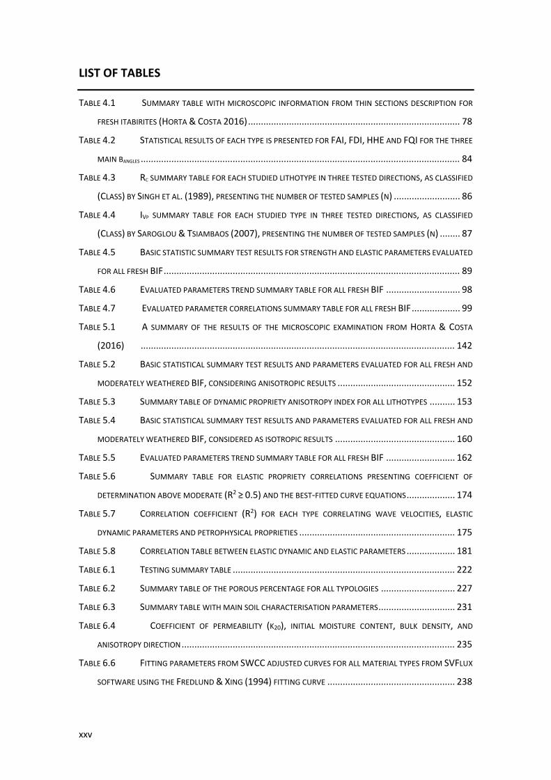
TABLE 4.1 SUMMARY TABLE WITH MICROSCOPIC INFORMATION FROM THIN SECTIONS DESCRIPTION FOR
FRESH ITABIRITES (HORTA & COSTA 2016) ................................................................................... 78
TABLE 4.2 STATISTICAL RESULTS OF EACH TYPE IS PRESENTED FOR FAI, FDI, HHE AND FQI FOR THE THREE
MAIN ΒANGLES ............................................................................................................................. 84
TABLE 4.3 RC SUMMARY TABLE FOR EACH STUDIED LITHOTYPE IN THREE TESTED DIRECTIONS, AS CLASSIFIED
(CLASS) BY SINGH ET AL. (1989), PRESENTING THE NUMBER OF TESTED SAMPLES (N) .......................... 86
TABLE 4.4 IVP SUMMARY TABLE FOR EACH STUDIED TYPE IN THREE TESTED DIRECTIONS, AS CLASSIFIED
(CLASS) BY SAROGLOU & TSIAMBAOS (2007), PRESENTING THE NUMBER OF TESTED SAMPLES (N) ........ 87
TABLE 4.5 BASIC STATISTIC SUMMARY TEST RESULTS FOR STRENGTH AND ELASTIC PARAMETERS EVALUATED
FOR ALL FRESH BIF .................................................................................................................... 89
TABLE 4.6 EVALUATED PARAMETERS TREND SUMMARY TABLE FOR ALL FRESH BIF ............................. 98
TABLE 4.7 EVALUATED PARAMETER CORRELATIONS SUMMARY TABLE FOR ALL FRESH BIF ................... 99
TABLE 5.1 A SUMMARY OF THE RESULTS OF THE MICROSCOPIC EXAMINATION FROM HORTA & COSTA
(2016) ........................................................................................................................... 142
TABLE 5.2 BASIC STATISTICAL SUMMARY TEST RESULTS AND PARAMETERS EVALUATED FOR ALL FRESH AND
MODERATELY WEATHERED BIF, CONSIDERING ANISOTROPIC RESULTS .............................................. 152
TABLE 5.3 SUMMARY TABLE OF DYNAMIC PROPRIETY ANISOTROPY INDEX FOR ALL LITHOTYPES .......... 153
TABLE 5.4 BASIC STATISTICAL SUMMARY TEST RESULTS AND PARAMETERS EVALUATED FOR ALL FRESH AND
MODERATELY WEATHERED BIF, CONSIDERED AS ISOTROPIC RESULTS ............................................... 160
TABLE 5.5 EVALUATED PARAMETERS TREND SUMMARY TABLE FOR ALL FRESH BIF ........................... 162
TABLE 5.6 SUMMARY TABLE FOR ELASTIC PROPRIETY CORRELATIONS PRESENTING COEFFICIENT OF
DETERMINATION ABOVE MODERATE (R2 ≥ 0.5) AND THE BEST-FITTED CURVE EQUATIONS ................... 174
TABLE 5.7 CORRELATION COEFFICIENT (R2) FOR EACH TYPE CORRELATING WAVE VELOCITIES, ELASTIC
DYNAMIC PARAMETERS AND PETROPHYSICAL PROPRIETIES ............................................................. 175
TABLE 5.8 CORRELATION TABLE BETWEEN ELASTIC DYNAMIC AND ELASTIC PARAMETERS ................... 181
TABLE 6.1 TESTING SUMMARY TABLE ....................................................................................... 222
TABLE 6.2 SUMMARY TABLE OF THE POROUS PERCENTAGE FOR ALL TYPOLOGIES ............................. 227
TABLE 6.3 SUMMARY TABLE WITH MAIN SOIL CHARACTERISATION PARAMETERS .............................. 231
TABLE 6.4 COEFFICIENT OF PERMEABILITY (K20), INITIAL MOISTURE CONTENT, BULK DENSITY, AND
ANISOTROPY DIRECTION ........................................................................................................... 235
TABLE 6.6 FITTING PARAMETERS FROM SWCC ADJUSTED CURVES FOR ALL MATERIAL TYPES FROM SVFLUX
SOFTWARE USING THE FREDLUND & XING (1994) FITTING CURVE .................................................. 238
xxvi
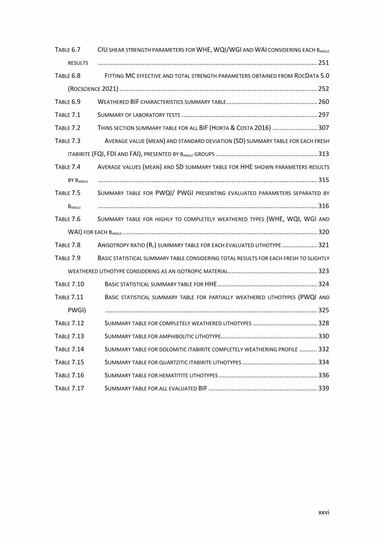
TABLE 6.7 CIU SHEAR STRENGTH PARAMETERS FOR WHE, WQI/WGI AND WAI CONSIDERING EACH ΒANGLE
RESULTS ........................................................................................................................... 251
TABLE 6.8 FITTING MC EFFECTIVE AND TOTAL STRENGTH PARAMETERS OBTAINED FROM ROCDATA 5.0
(ROCSCIENCE 2021) ............................................................................................................... 252
TABLE 6.9 WEATHERED BIF CHARACTERISTICS SUMMARY TABLE ................................................... 260
TABLE 7.1 SUMMARY OF LABORATORY TESTS ............................................................................ 297
TABLE 7.2 THINS SECTION SUMMARY TABLE FOR ALL BIF (HORTA & COSTA 2016) ......................... 307
TABLE 7.3 AVERAGE VALUE (MEAN) AND STANDARD DEVIATION (SD) SUMMARY TABLE FOR EACH FRESH
ITABIRITE (FQI, FDI AND FAI), PRESENTED BY ΒANGLE GROUPS ......................................................... 313
TABLE 7.4 AVERAGE VALUES (MEAN) AND SD SUMMARY TABLE FOR HHE SHOWN PARAMETERS RESULTS
BY ΒANGLE ........................................................................................................................... 315
TABLE 7.5 SUMMARY TABLE FOR PWQI/ PWGI PRESENTING EVALUATED PARAMETERS SEPARATED BY
ΒANGLE ........................................................................................................................... 316
TABLE 7.6 SUMMARY TABLE FOR HIGHLY TO COMPLETELY WEATHERED TYPES (WHE, WQI, WGI AND
WAI) FOR EACH ΒANGLE ............................................................................................................. 320
TABLE 7.8 ANISOTROPY RATIO (RC) SUMMARY TABLE FOR EACH EVALUATED LITHOTYPE .................... 321
TABLE 7.9 BASIC STATISTICAL SUMMARY TABLE CONSIDERING TOTAL RESULTS FOR EACH FRESH TO SLIGHTLY
WEATHERED LITHOTYPE CONSIDERING AS AN ISOTROPIC MATERIAL .................................................. 323
TABLE 7.10 BASIC STATISTICAL SUMMARY TABLE FOR HHE ........................................................ 324
TABLE 7.11 BASIC STATISTICAL SUMMARY TABLE FOR PARTIALLY WEATHERED LITHOTYPES (PWQI AND
PWGI) ....................................................................................................................... 325
TABLE 7.12 SUMMARY TABLE FOR COMPLETELY WEATHERED LITHOTYPES .................................... 328
TABLE 7.13 SUMMARY TABLE FOR AMPHIBOLITIC LITHOTYPE ...................................................... 330
TABLE 7.14 SUMMARY TABLE FOR DOLOMITIC ITABIRITE COMPLETELY WEATHERING PROFILE .......... 332
TABLE 7.15 SUMMARY TABLE FOR QUARTZITIC ITABIRITE LITHOTYPES .......................................... 334
TABLE 7.16 SUMMARY TABLE FOR HEMATITITE LITHOTYPES ....................................................... 336
TABLE 7.17 SUMMARY TABLE FOR ALL EVALUATED BIF ............................................................. 339
xxvii
LIST OF GRAPHS
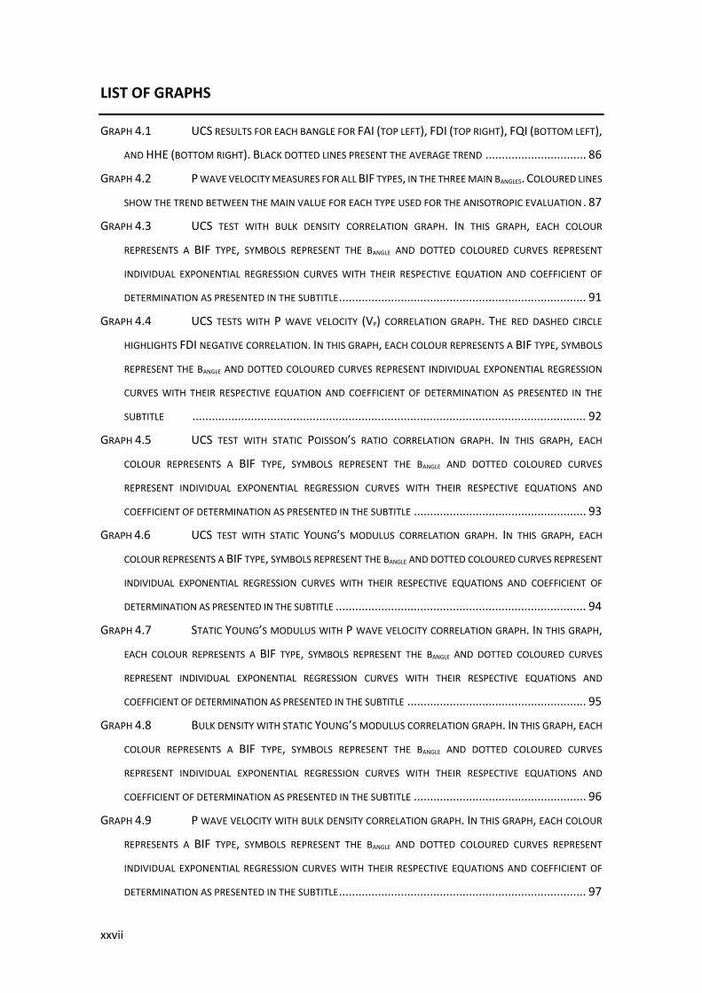
GRAPH 4.1 UCS RESULTS FOR EACH ΒANGLE FOR FAI (TOP LEFT), FDI (TOP RIGHT), FQI (BOTTOM LEFT),
AND HHE (BOTTOM RIGHT). BLACK DOTTED LINES PRESENT THE AVERAGE TREND ............................... 86
GRAPH 4.2 P WAVE VELOCITY MEASURES FOR ALL BIF TYPES, IN THE THREE MAIN ΒANGLES. COLOURED LINES
SHOW THE TREND BETWEEN THE MAIN VALUE FOR EACH TYPE USED FOR THE ANISOTROPIC EVALUATION . 87
GRAPH 4.3 UCS TEST WITH BULK DENSITY CORRELATION GRAPH. IN THIS GRAPH, EACH COLOUR
REPRESENTS A BIF TYPE, SYMBOLS REPRESENT THE ΒANGLE AND DOTTED COLOURED CURVES REPRESENT
INDIVIDUAL EXPONENTIAL REGRESSION CURVES WITH THEIR RESPECTIVE EQUATION AND COEFFICIENT OF
DETERMINATION AS PRESENTED IN THE SUBTITLE ............................................................................ 91
GRAPH 4.4 UCS TESTS WITH P WAVE VELOCITY (VP) CORRELATION GRAPH. THE RED DASHED CIRCLE
HIGHLIGHTS FDI NEGATIVE CORRELATION. IN THIS GRAPH, EACH COLOUR REPRESENTS A BIF TYPE, SYMBOLS
REPRESENT THE ΒANGLE AND DOTTED COLOURED CURVES REPRESENT INDIVIDUAL EXPONENTIAL REGRESSION
CURVES WITH THEIR RESPECTIVE EQUATION AND COEFFICIENT OF DETERMINATION AS PRESENTED IN THE
SUBTITLE ......................................................................................................................... 92
GRAPH 4.5 UCS TEST WITH STATIC POISSON’S RATIO CORRELATION GRAPH. IN THIS GRAPH, EACH
COLOUR REPRESENTS A BIF TYPE, SYMBOLS REPRESENT THE ΒANGLE AND DOTTED COLOURED CURVES
REPRESENT INDIVIDUAL EXPONENTIAL REGRESSION CURVES WITH THEIR RESPECTIVE EQUATIONS AND
COEFFICIENT OF DETERMINATION AS PRESENTED IN THE SUBTITLE ..................................................... 93
GRAPH 4.6 UCS TEST WITH STATIC YOUNG’S MODULUS CORRELATION GRAPH. IN THIS GRAPH, EACH
COLOUR REPRESENTS A BIF TYPE, SYMBOLS REPRESENT THE ΒANGLE AND DOTTED COLOURED CURVES REPRESENT
INDIVIDUAL EXPONENTIAL REGRESSION CURVES WITH THEIR RESPECTIVE EQUATIONS AND COEFFICIENT OF
DETERMINATION AS PRESENTED IN THE SUBTITLE ............................................................................. 94
GRAPH 4.7 STATIC YOUNG’S MODULUS WITH P WAVE VELOCITY CORRELATION GRAPH. IN THIS GRAPH,
EACH COLOUR REPRESENTS A BIF TYPE, SYMBOLS REPRESENT THE ΒANGLE AND DOTTED COLOURED CURVES
REPRESENT INDIVIDUAL EXPONENTIAL REGRESSION CURVES WITH THEIR RESPECTIVE EQUATIONS AND
COEFFICIENT OF DETERMINATION AS PRESENTED IN THE SUBTITLE ....................................................... 95
GRAPH 4.8 BULK DENSITY WITH STATIC YOUNG’S MODULUS CORRELATION GRAPH. IN THIS GRAPH, EACH
COLOUR REPRESENTS A BIF TYPE, SYMBOLS REPRESENT THE ΒANGLE AND DOTTED COLOURED CURVES
REPRESENT INDIVIDUAL EXPONENTIAL REGRESSION CURVES WITH THEIR RESPECTIVE EQUATIONS AND
COEFFICIENT OF DETERMINATION AS PRESENTED IN THE SUBTITLE ..................................................... 96
GRAPH 4.9 P WAVE VELOCITY WITH BULK DENSITY CORRELATION GRAPH. IN THIS GRAPH, EACH COLOUR
REPRESENTS A BIF TYPE, SYMBOLS REPRESENT THE ΒANGLE AND DOTTED COLOURED CURVES REPRESENT
INDIVIDUAL EXPONENTIAL REGRESSION CURVES WITH THEIR RESPECTIVE EQUATIONS AND COEFFICIENT OF
DETERMINATION AS PRESENTED IN THE SUBTITLE ............................................................................ 97
xxvii
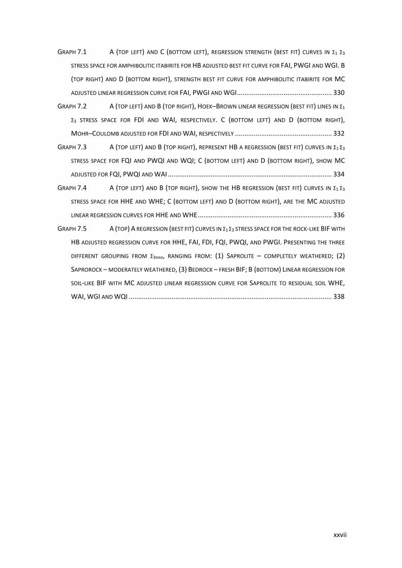
GRAPH 7.1 A (TOP LEFT) AND C (BOTTOM LEFT), REGRESSION STRENGTH (BEST FIT) CURVES IN Σ1 Σ3
STRESS SPACE FOR AMPHIBOLITIC ITABIRITE FOR HB ADJUSTED BEST FIT CURVE FOR FAI, PWGI AND WGI. B
(TOP RIGHT) AND D (BOTTOM RIGHT), STRENGTH BEST FIT CURVE FOR AMPHIBOLITIC ITABIRITE FOR MC
ADJUSTED LINEAR REGRESSION CURVE FOR FAI, PWGI AND WGI ................................................... 330
GRAPH 7.2 A (TOP LEFT) AND B (TOP RIGHT), HOEK–BROWN LINEAR REGRESSION (BEST FIT) LINES IN Σ1
Σ3 STRESS SPACE FOR FDI AND WAI, RESPECTIVELY. C (BOTTOM LEFT) AND D (BOTTOM RIGHT),
MOHR–COULOMB ADJUSTED FOR FDI AND WAI, RESPECTIVELY .................................................... 332
GRAPH 7.3 A (TOP LEFT) AND B (TOP RIGHT), REPRESENT HB A REGRESSION (BEST FIT) CURVES IN Σ1 Σ3
STRESS SPACE FOR FQI AND PWQI AND WQI; C (BOTTOM LEFT) AND D (BOTTOM RIGHT), SHOW MC
ADJUSTED FOR FQI, PWQI AND WAI ........................................................................................ 334
GRAPH 7.4 A (TOP LEFT) AND B (TOP RIGHT), SHOW THE HB REGRESSION (BEST FIT) CURVES IN Σ1 Σ3
STRESS SPACE FOR HHE AND WHE; C (BOTTOM LEFT) AND D (BOTTOM RIGHT), ARE THE MC ADJUSTED
LINEAR REGRESSION CURVES FOR HHE AND WHE ........................................................................ 336
GRAPH 7.5 A (TOP) A REGRESSION (BEST FIT) CURVES IN Σ1 Σ3 STRESS SPACE FOR THE ROCK-LIKE BIF WITH
HB ADJUSTED REGRESSION CURVE FOR HHE, FAI, FDI, FQI, PWQI, AND PWGI. PRESENTING THE THREE
DIFFERENT GROUPING FROM Σ3MAX, RANGING FROM: (1) SAPROLITE – COMPLETELY WEATHERED; (2)
SAPROROCK – MODERATELY WEATHERED, (3) BEDROCK – FRESH BIF; B (BOTTOM) LINEAR REGRESSION FOR
SOIL-LIKE BIF WITH MC ADJUSTED LINEAR REGRESSION CURVE FOR SAPROLITE TO RESIDUAL SOIL WHE,
WAI, WGI AND WQI ............................................................................................................. 338
xxix
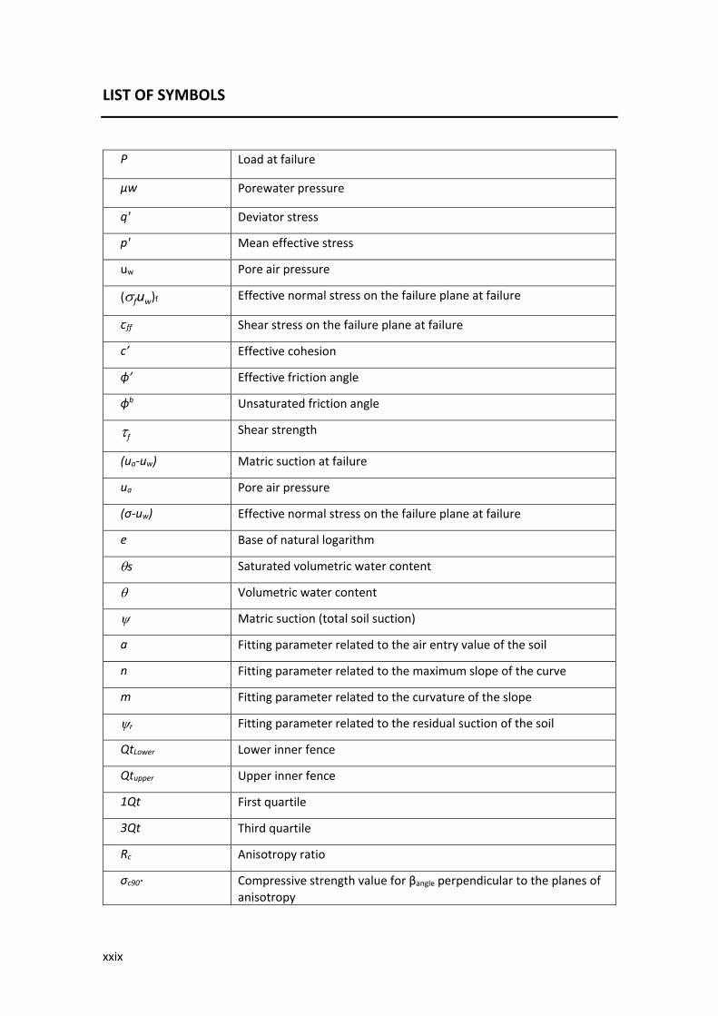
LIST OF SYMBOLS
P Load at failure
μw Porewater pressure
q' Deviator stress
p' Mean effective stress
uw Pore air pressure
(σfuw)f Effective normal stress on the failure plane at failure
ꞇff Shear stress on the failure plane at failure
c’ Effective cohesion
ɸ’ Effective friction angle
ɸb Unsaturated friction angle
τf Shear strength
(ua-uw) Matric suction at failure
ua Pore air pressure
(σ-uw) Effective normal stress on the failure plane at failure
e Base of natural logarithm
θs Saturated volumetric water content
θ Volumetric water content
ψ Matric suction (total soil suction)
a Fitting parameter related to the air entry value of the soil
n Fitting parameter related to the maximum slope of the curve
m Fitting parameter related to the curvature of the slope
ψr Fitting parameter related to the residual suction of the soil
QtLower Lower inner fence
Qtupper Upper inner fence
1Qt First quartile
3Qt Third quartile
Rc Anisotropy ratio
σc90° Compressive strength value for βangle perpendicular to the planes of anisotropy
xxx
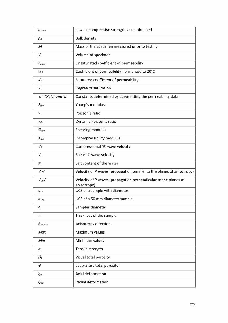
σcmin Lowest compressive strength value obtained
ρb Bulk density
M Mass of the specimen measured prior to testing
V Volume of specimen
kunsat Unsaturated coefficient of permeability
k20 Coefficient of permeability normalised to 20°C
Ks Saturated coefficient of permeability
S Degree of saturation
‘a’, ‘b’, ‘c’ and ‘p’ Constants determined by curve fitting the permeability data
Edyn Young’s modulus
ν Poisson’s ratio
νdyn Dynamic Poisson’s ratio
Gdyn Shearing modulus
Kdyn Incompressibility modulus
VP Compressional ‘P’ wave velocity
Vs Shear ‘S’ wave velocity
π Salt content of the water
Vp0° Velocity of P waves (propagation parallel to the planes of anisotropy)
Vp90° Velocity of P waves (propagation perpendicular to the planes of anisotropy)
σcd UCS of a sample with diameter
σc50 UCS of a 50 mm diameter sample
d Samples diameter
t Thickness of the sample
βangles Anisotropy directions
Max Maximum values
Min Minimum values
σt Tensile strength
Øb Visual total porosity
Ø Laboratory total porosity
ξax Axial deformation
ξrad Radial deformation
xxxi
ACKNOWLEDGEMENTS
The author thanks thesis supervisor Phil Dight and co-supervisors Eduardo Marques and
Ken Mercer for their support and orientation during this long journey. Also, thanks to Vale S.A.
for their permission to present this thesis and sponsorship of the research. The author’s
appreciation extends to the ACG team in the name of Christine Neskudla, Josephine Ruddle,
Garth Doig and Stefania Woodward for the amazing support and for making me feel part of the
ACG family, and to former ACG staff member Ariel Hsieh for the support and discussions.
Appreciation is extended for all ‘giants’, Paulo Franca, Rene Viel, Peter Stacey, John Read,
Waldyr Oliveira, Flavio Afonso Oxy, Vitor Suckau, Cesar Grandchamp, Rodrigo Figueiredo, Fabio
Magalhães and Sergio Brito (in memoriam) for their contributions in my career and thesis
reviews, and to Laura Horta and Pedro Henrique Alves for precious evaluations and support
during thesis development.
xxxii
DEDICATION
This thesis is dedicated to my mother (in memoriam) for her endless love, sacrifice, prayers, and
support.
Also, to my beloved father and mother in law for their endless love, support, prayers, and
encouragement.
To Mariana, Luiza and Julia for their deep love, emotional support, and sacrifice. I promise to
reward you all very soon!
“If I have seen further, it is by standing upon the shoulders of giants” Isaac Newton, 1675
xxxiii
AUTHORSHIP DECLARATION: CO-AUTHORED PUBLICATIONS
This thesis contains work that has been published and work prepared for publication.
Details of the work: An overview of the weathering process and preliminary density and UCS correlations for fresh itabirites in Vale mines on the western side of the Iron Quadrangle, Brazil This paper presents a review of the geological, geotechnical, and weathering characteristics of the itabirites, and early results for the fresh BIF evaluations from the PhD thesis research. The results showed that to evaluate the bulk density and unconfined compressive strength (UCS) correlation, not only the porosity but also the geological features should be considered, as they are responsible for data dispersion. However, the presented data suggested a trend that provides the confidence to develop advanced studies and data population increment to establish a proper correlation to support a reliable UCS index method. Location in thesis: Appendix I Student contribution to work: 70%
Co-author signatures and dates:
Phil Dight Date: June 25, 2021
Ken Mercer Date: June 21, 2021
Eduardo Marques Date: June 21, 2021
xxxiv
Details of the work: Weathered banded iron formations in Vale iron ore mines on the western side of the Iron Quadrangle, Brazil: weak hematitite and weathered argillaceous itabirite geotechnical characteristics and implications of matric suction effects on slope stability This paper presents a review of the geological and weathering characteristics and related geomechanical and strength assessments of two important lithotypes commonly associated with slope failure mechanisms in Vale mines: weathered argillaceous itabirite (WAI) and weak hematitite (WHE). These studies are based on early research results from the PhD thesis. The results show that minor changes in bulk density, rock fabric, and the percentage of clay minerals lead to distinct geomechanical characteristics in terms of plasticity, intact rock strength and mainly matric suction effects. These changes influence both the shear strength and intact rock behaviour and consequently the overall slope stability as shown in a preliminary insight into the open pit slope design for short and long-term considerations. Location in thesis: Appendix II Student contribution to work: 70% Co-author signatures and dates:
Phil Dight Date: June 25, 2021
Ken Mercer Date: June 21, 2021
Eduardo Marques Date: June 21, 2021
Student signature: Date: June 21, 2021
I, Phil Dight certify that the student statements regarding their contribution to each of the works listed above are correct.
Coordinating supervisor signature: Date: June 25, 2021
1
CHAPTER 1. INTRODUCTION
1.1 PROBLEM STATEMENT
In recent decades, a booming worldwide iron ore market has pressed iron ore mines to increase
their production by developing innovative technologies, opening new mines, and expanding
existing mines, not only in width but mainly in depth, to meet this high demand.
In this period, iron ore mines located in the Iron Quadrangle, Brazil were especially affected by
environmental and social pressures to reduce expansion of the mining footprint. The expansion
was based on technological development and increase of depth in existing mines. With pit
depths going beyond 500 m, the former pit designs, based on soil-like behaviour for friable
material, are no longer valid.
These iron ore mines are developed in banded iron formations (BIF) deposits, originally
described by Dorr (1969) as a high-grade ore, called hematite (most recently denominated as
hematitite) and a low-grade ore, called itabirite. The original mineralogical composition of
non-iron bands, consisting of dolomitic, amphibolitic and quartzitic layers are used to
differentiate itabirite types. In addition, those lithotypes are the hardest (fresh) BIF seen in Iron
Quadrangle iron ore mines that, under multiple geological process (mainly weathering), resulted
in multiple rock types with low strength.
Brazilian iron ore mines exhibit weathering profiles that can reach over 400 m in depth. This
means that for shallow mines (less than 400 m depth) slopes are composed mainly of residual
soil to moderately weathered rocks with a minor presence of fresh rocks and in deeper mines
(more than 400 m deep) the slopes are composed of a range of residual soils to fresh rocks. For
geotechnical purposes, this depth division is appropriate for a geomechanical approach and
these mines must be considered as saprolite deep deposits of BIF where the typical weathering
profile characteristic must be established and considered.
For shallow mines, where the rocks exhibit soil mechanics behaviour, the slope design approach
and the identification of possible failure mechanisms is largely based on applying classical soil
mechanics principals as well as historical trial-and-error experience. While this approach has
been largely satisfactory, there are nevertheless several key geotechnical issues that are still not
well understood, and there have been continued instances of large slope failures which have
resulted in significant disruptions to the mines.
For the proposed deeper mines, the increase in fresh and hard rock at the toes of the slopes
presents new challenges for subsequent geotechnical designs and slope failure assessments,
2
such as the application of rock mechanics, definition of rock mass and related discontinuities
important for failure mechanism identification.
Based on these facts the research will address the main aspects, described below, to determine
the boundary between residual soil, saprolite, saprorock and bedrock for BIF weathering profiles
to establish the best practices for slope design analysis and evaluations of failure mechanisms
at different weathering profile horizons.
Bedrock horizon – hard and fresh rock geotechnical behaviour characterisation
With the deepening of iron ore mines, there will be an increase in the percentage of hard and
fresh rocks exposed (bedrock), which poses new challenges to geotechnical teams to develop
slope designs and evaluate failure mechanisms using rock mechanics principles, breaking some
paradigms used over the last decades of operation in weak rocks. As such, there will be limited
precedence to follow and few numbers of failure mechanism studies on these hard rock masses
that could provide previous experiences.
For these hard rocks’ masses, it is crucial to ensure a good evaluation of intact rock strength and
discontinuities in order to define the rock mass strength and understand deformation behaviour
for slopes composed of a quite complex arrangement of different rock strength and elastic
materials.
The BIF heterogeneity and associated anisotropic effects on intact rock proprieties poses an
extra challenge, due to the heterogeneity produced by typical itabirites compositional
metamorphic banding that could induce significant changes on intact rock strength and elastic
parameters which can even determine failure mechanisms.
Saprorock horizon– partially weathered, a mix of weak and hard rock geotechnical behaviour
characterisation
As a transition between fresh to completely weathered rocks, these moderately to highly
weathered types can reach hundreds of metres of thickness and behave as a rock or soil
depending on intact rock strength and stress level. This ambiguous behaviour affects not only
the choice of laboratorial tests but also the approach necessary to characterise and evaluate
failure mechanism which involves the appropriate use of rock or soil mechanics principles.
It is also important to assess the geotechnical parameters for partially weathered rocks, defined
as saprorock and configuring a mix of hard and weak material.
Saprolite horizon – weak and completely weathered to residual soil geotechnical behaviour
characterisation
For completely weathered rocks to residual soil, these low strength rocks with soil-like behaviour
are the result of alteration of the original fresh rock imposed in part of the hypogene and
3
supergene iron enrichment process but mainly by weathering and could be defined as typical
saprolite as show in this research.
In shallow mines, the approach in dealing with weak rocks and slope design has largely been
based on adopting soil mechanics principles and past experiences. Studies by Costa (2009), Sá
(2010) and Martin and Stacey (2018) suggest that some failure mechanisms have specific
characteristics for weak leached materials, and that the application of classical soil mechanics
principles does not enable failure mechanisms to be fully understood, while rock mechanics
concepts are also not fully applicable. It is therefore apparent that an appropriate geotechnical
approach is required to address these rock types.
Intact rock and shear strength parameters for these designs are normally based on a limited
number of soil laboratory tests (such as triaxial and direct shear) or derived from adapted
geomechanical classifications. While this approach has been mostly successful, it appears they
may be conservative. In spite of that, there have been examples of large slope failures not
captured by these design approaches that have had significant negative impacts for mine
production and in some cases resulted in fatalities.
It is also recognised that failure mechanisms in weak rock slopes are controlled mainly by intact
rock shear strength and anisotropic effects, as well as secondary factors such as structural
control and water content. The situation is particularly challenging when considering the
stratigraphic position and/or tectonic settings of these weak and weathered rocks, which are
very often located at the toe of high slopes, where the stress is concentrated. To address this
issue, historically geotechnical engineers leave a ‘buttress’ at the toe of the wall, resulting in a
loss of reserves.
Additionally, the lack of knowledge of pore pressure effects (in situ and laboratory tests) and the
behaviour of partially saturated or unsaturated conditions for these weak materials increases
the challenge as the porewater pressure influence (positive or negative) is not properly
understood and considered in slope stability analyses.
Generally, in iron ore mines, the slope stability analyses are performed using saturated
parameters, although the slope may remain unsaturated, which could represent a conservative
approach or using unsaturated parameters that could represent a risky approach. For both
cases, the result leads to a difference between site conditions and the analytical results.
1.2 RESEARCH OBJECTIVES
The geological focus of this research is to evaluate how the weathering and other iron
enrichment processes (supergene and hypogene) have affected the geomechanical properties
of BIF for all materials found in a complete weathering profile. To reach this aim, a geological
4
and geotechnical approach was used to determine the weathering profile horizons and zones,
providing reliable intact rock strength and elastic parameter based on site investigation and
laboratory tests, establishing empirical correlations (graphs and/or equations) between these
parameters, petrophysical and geological features, and finally addressing the consequent
importance of these processes on the slope stability for iron ore open pit mines
To address these goals, three primary objectives were established as summarised below:
Objective 1 – Evaluate, for all BIF types, geological and petrophysical macrofeatures and
microfeatures associated with geomechanical properties considering the anisotropy and
heterogeneity characteristics
• Define the most important geological, petrophysical features, and geotechnical
parameters responsible for the geomechanical behaviour of each weathering profile
horizon.
• Define the correlations between geological features and petrographic characteristics
(mineralogy and fabric) with the geomechanical parameters for each individual BIF
weathering profile horizons.
Objective 2 – Evaluate, for all BIF types, the intact rock strength and elastic parameters
considering the anisotropy and heterogeneity characteristics
• Define the most appropriate laboratory test type for each weathering horizon defining
remarks, restrictions, and results variation.
• Define how BIF intact rock and shear strength, and elastic parameters (dynamic and
static) changes from different BIF types at multiple weathering horizons.
• Define the strength anisotropy ratio for each BIF type and weathering horizon.
• Define reliable empirical correlations (graphs and/or equations), considering the most
important petrophysical and geomechanical parameters, for each BIF type and
weathering horizon.
• Evaluate the saturated and unsaturated behaviour considering the porewater pressure
(matric suction) effects for BIF soil types.
Objective 3 – Evaluate the complete BIF weathering profile characteristics, setting the
boundaries, establishing a geological and geomechanical characterisation
• Define the typical BIF weathering profile and show how the weathering affects each
BIF type resulting in different weathering profiles.
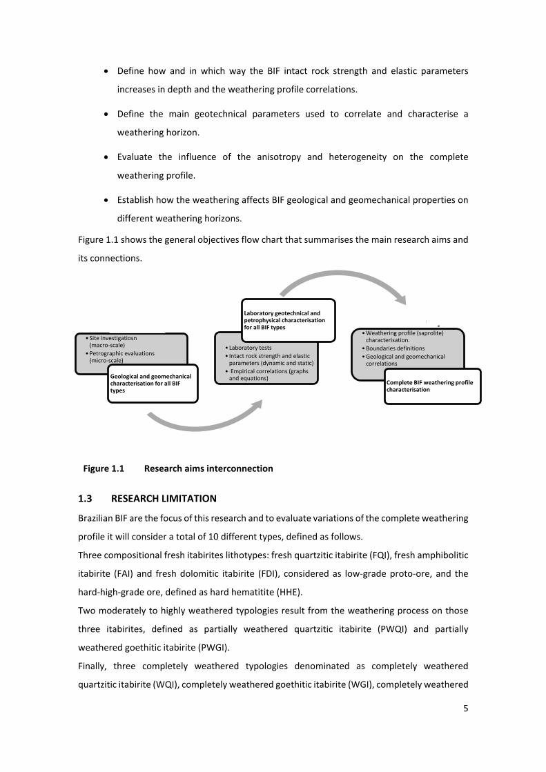
5
• Define how and in which way the BIF intact rock strength and elastic parameters
increases in depth and the weathering profile correlations.
• Define the main geotechnical parameters used to correlate and characterise a
weathering horizon.
• Evaluate the influence of the anisotropy and heterogeneity on the complete
weathering profile.
• Establish how the weathering affects BIF geological and geomechanical properties on
different weathering horizons.
Figure 1.1 shows the general objectives flow chart that summarises the main research aims and
its connections.
1Figure 1.1 Research aims interconnection
1.3 RESEARCH LIMITATION
Brazilian BIF are the focus of this research and to evaluate variations of the complete weathering
profile it will consider a total of 10 different types, defined as follows.
Three compositional fresh itabirites lithotypes: fresh quartzitic itabirite (FQI), fresh amphibolitic
itabirite (FAI) and fresh dolomitic itabirite (FDI), considered as low-grade proto-ore, and the
hard-high-grade ore, defined as hard hematitite (HHE).
Two moderately to highly weathered typologies result from the weathering process on those
three itabirites, defined as partially weathered quartzitic itabirite (PWQI) and partially
weathered goethitic itabirite (PWGI).
Finally, three completely weathered typologies denominated as completely weathered
quartzitic itabirite (WQI), completely weathered goethitic itabirite (WGI), completely weathered
Objective 1
Objective 2
Objective 3 • Site investigatiosn
(macro-scale)• Petrographic evaluations
(micro-scale)
Geological and geomechanical characterisation for all BIF types
• Laboratory tests• Intact rock strength and elastic
parameters (dynamic and static)• Empirical correlations (graphs
and equations)
Laboratory geotechnical and petrophysical characterisation for all BIF types
• Weathering profile (saprolite) characterisation.
• Boundaries definitions• Geological and geomechanical
correlations
Complete BIF weathering profile characterisation
6
argillaceous itabirite (WAI) defined as poor itabirites, and the weak hematitite (WHE) defined as
rich friable ore.
Those rocks represent more than 60% of the final slope exposed rocks (another 40% is composed
of country rocks) and more than 90% of BIF type expositions. The semi compact hematitite, was
not evaluated in this thesis owing to the reduced geotechnical importance and spatial
distribution in iron ore mines.
An important limitation is referred to the genesis of the weak material and correlated loss of
strength during geological events and time. This research will concentrate on physical and
chemical changes posed by the weathering process, considering this event the most important
process responsible for reducing the intact rock shear strength of the BIF as described by Ribeiro
(2002a and 2003). However, there are other geological processes such as supergene and
hypogene iron enrichment, tectonic events and metamorphism that could change the rock
strength. With this simplification, it was possible to establish a direct correlation between intact
rock characteristics and strength variations at depth with distinct levels of weathering
throughout the weathering profile.
The research will also focus on the typical BIF heterogeneity attributed to the compositional
metamorphic banding or foliation, and its anisotropic effects in the intact rock strength. For this
evaluation, discontinuities and rock mas strength parameters were not considered, even though
considering these to be crucial for the complete understanding of slope stability behaviour for
residual soil or saprolite that contain relict structures and discontinuities in certain areas.
In addition, discontinuity characterisation and correlation with rock mass strength are not
considered in this research, which focuses on intact rock strength. Nevertheless, the importance
of the structural characteristics for slope stability behaviour, for bedrock and saprorock analyses
is recognised.
The studied mines are part of Vale’s south ferrous division and include 15 mines located in the
centre of Minas Gerais state, Brazil, as shown in Figure 1.2. The mines are: Águas Claras (MAC),
Mutuca (MUT), Mar Azul (MAZ), Capão Xavier (CPX), Tamanduá (TAM), Capitão do Mato (CMT),
Abóboras (ABO), Galinheiro (GAL), Sapecado (SAP), Pico (PIC), Córrego do Feijão (CFJ), Jangada
(JGD), João Pereira (JPE), Alto Bandeira (BAN) and Fábrica (FAB). The mines which have been
studied are located in Iron Quadrangle western low strain domain and green schist metamorphic
zone (Rosière et al. 1993). Evaluations in different tectonic settings and different iron deposits
must be made considering these geological influences.
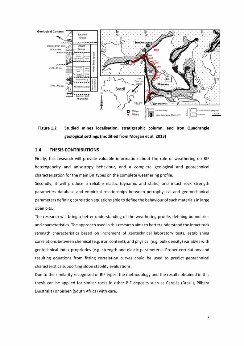
7
2 Figure 1.2 Studied mines localisation, stratigraphic column, and Iron Quadrangle
geological settings (modified from Morgan et al. 2013)
1.4 THESIS CONTRIBUTIONS
Firstly, this research will provide valuable information about the role of weathering on BIF
heterogeneity and anisotropy behaviour, and a complete geological and geotechnical
characterisation for the main BIF types on the complete weathering profile.
Secondly, it will produce a reliable elastic (dynamic and static) and intact rock strength
parameters database and empirical relationships between petrophysical and geomechanical
parameters defining correlation equations able to define the behaviour of such materials in large
open pits.
The research will bring a better understanding of the weathering profile, defining boundaries
and characteristics. The approach used in this research aims to better understand the intact rock
strength characteristics based on increment of geotechnical laboratory tests, establishing
correlations between chemical (e.g. iron content), and physical (e.g. bulk density) variables with
geotechnical index proprieties (e.g. strength and elastic parameters). Proper correlations and
resulting equations from fitting correlation curves could be used to predict geotechnical
characteristics supporting slope stability evaluations.
Due to the similarity recognised of BIF types, the methodology and the results obtained in this
thesis can be applied for similar rocks in other BIF deposits such as Carajás (Brazil), Pilbara
(Australia) or Sishen (South Africa) with care.
SDB
CH
SM
BD
8
Finally, the thesis expected to contribute to optimise current slope failure mechanism
evaluation, final slope design, and slope safety practices, improving operational productivity,
thereby ensuring necessary safety operations and stability in iron ore open pits.
1.5 THESIS ORGANISATION
This thesis is organised in accordance with The University of Western Australia’s Doctor of
Philosophy rules for the content and format of a thesis presented as a series of papers. It is
organised into nine chapters, which following this introductory Chapter 1, where the problem
statement is presented, the main objectives and expected results, thesis limitations and its
organisation are presented.
Chapter 2 presents a brief summary of the most relevant literature overview, separated by topic.
To reduce the repetition, this chapter presents a general literature review of each topic
discussed in this thesis. The specific and detailed used literature review are presented separately
in each chapter. Chapter 3 presents the site investigations, laboratory tests, and methodology
necessary to develop the thesis.
The following four chapters constitute the main portion of the thesis and present the results,
discussions, and conclusions from unpublished manuscripts. Each chapter stands alone and
covers one or more topics of the research objectives (Section 1.2) and were written to allow the
audience to have a complete understanding of the topics without the necessity to read the other
chapters. This configuration could lead to repetition, especially in the first part of each chapter.
For this reason, some editorial adjustments were made to improve consistency and reduce
repetition, mainly in Chapter 2 (Literature Review) and Chapter 3 (Methodology). Additionally,
thanks to editorial purposes, some chapters could be split into more than one article due to
elevate number of words and size of the figures and graphs contained.
Additionally, the two published papers are presented in the appendices section, also in order to
reduce the repetition. Appendix I (Costa et al. 2015), is titled ‘An overview of the weathering
process and preliminary bulk density and UCS correlations for fresh itabirites in Vale mines on
the western side of the Iron Quadrangle, Brazil’. It is a peer reviewed paper presented and
published in 2015 in Iron Ore, AusIMM and CSIRO conference proceedings – Perth, Australia,
focusing on the geological and geotechnical setting of fresh BIF and weathering profile, thesis
early results regarding the samples grouping, the techniques used to define the outliers, and the
correlation between iron content, bulk density and UCS tests for fresh itabirites and hard
hematitite.
Appendix II (Costa et al. 2015), is titled ‘Weathered banded iron formations in Vale iron ore
mines on the western side of the Iron Quadrangle, Brazil: weak hematitite and weathered
9
argillaceous itabirite geotechnical characteristics and implications of matric suction effects on
slope stability’. It is a peer reviewed paper presented and published in 2015 in the Slope Stability
2015, International Symposium proceedings – SS03, Cape Town, South Africa, focusing on the
geological and geotechnical setting of weak hematitites and completely weathered argillaceous
itabirites, thesis early results regarding the weak rock saturated and unsaturated soil behaviour,
porewater pressure effects and a slope stability case study evaluation considering this influence.
Chapter 4 is denominated ‘Intact rock strength characteristics and elastic static properties of
fresh Brazilian banded iron formations’. This chapter presents the first unpublished manuscript.
It presents the geological and geotechnical setting of fresh BIF, final considerations about the
relationship between physical proprieties, intact rock strength parameters and static elastic
modulus, and defines the influence of anisotropy ratio based on intact rock strength and
established empirical correlations equations for the most important parameters recognised.
Chapter 5 is denominated ‘Petrophysical characteristics and elastic dynamic properties of fresh
to moderately weathered Brazilian banded iron formations’. This chapter presents the second
unpublished manuscript. It presents final considerations about the relationship between intact
rock strength, petrophysical proprieties, VP and Vs, and dynamic elastic modulus, and the effects
of anisotropy ratio on these rocks based on wave propagation.
Chapter 6 is denominated ‘Weak rock behaviour of highly to completely weathered Brazilian
banded iron formations’. This chapter presents the third unpublished manuscript. It presents
the BIF weak rock and soil-like types behaviour for saturated and unsaturated conditions,
defines the influence of anisotropy ratio on these soil types considering the intact rock strength,
and presents the shear strength parameters for all types and porewater pressure effects.
Chapter 7 is denominated ‘Weathering profile, intact rock strength and elastic characteristics of
Brazilian banded iron formations’. This chapter presents the fourth unpublished manuscript. It
presents the geological and geotechnical setting from fresh to completely weathered BIF
defining the weathering profiles’ main characteristics and boundary between the weathering
horizons, final considerations about the relationship between petrophysical proprieties, intact
rock strength parameters and elastic modulus, and defines the influence of anisotropy ratio on
these rocks considering the intact rock strength for all weathering profiles.
Chapter 8 concludes the thesis by presenting the main discussions and findings reached from
the research development. Finally, Chapter 9 suggests the next steps and future research
advance.

10
11
CHAPTER 2. LITERATURE REVIEW
2.1 REGIONAL GEOLOGICAL SETTINGS
The focus area is located at the western part of the Iron Quadrangle on the southern border of
São Francisco Craton. The mines are situated on Moeda (SM) and Don Bosco (SDB) Synclines and
Curral Homocline range (CH) (Figure 1.1).
The structure is delineated by a roughly quadrangular arrangement, with Paleoproterozoic BIF
of the Minas Supergroup, as proposed by Dorr (1969). This supergroup is composed of hundreds
of metres of iron-rich metamorphic rocks belonging to the Itabira group/Cauê Formation. The
Minas Supergroup comprises, from the bottom to the top: Caraça, Itabira, Piracicaba and Sabará
groups; a sequence of psammitic and pelitic rocks, also defined by Dorr (1969); all of which are
overlain by the Itacolomi group. Below this sequence are the Archean greenstone belt terrains
of the Rio das Velhas Supergroup and domes of Archean and Proterozoic crystalline rocks
(Machado & Carneiro 1992, Machado et al. 1989, and Noce 1995).
The Cauê Formation (Itabira Group), which hosts the BIF, is a marine chemical sequence 350 m
thick, dated 2.4 ± 0.19 Gyr by Babinski et al. (1995).
The regional structure is the result of two major deformational super-positional events, as
proposed by Chemale Jr et al. (1994). The first event produced the nucleation of regional
synclines in the uplift of the gneissic domes during the Transamazonian Orogenesis (2.1–2 Gyr),
and the second is related to an east–west verging thrust fault belt of Pan African/Brazilian age
(0.8–0.6 Gyr) described by Marshak & Alkmim (1989). This last event deformed the earlier
structures and was mainly responsible for the deformational gradient. Hertz (1978) described
an eastward increase in the metamorphic grade from green schist to lower amphibolite facies
following the deformational gradient.
The mines which have been studied are located in the western low strain domain and green
schist metamorphic zone, formed in the Transamazonian event. The main trend of the synclines
is north–south, but the structure has also been deformed around Bação dome (BD). It is also
interconnected with Dom Bosco Syncline to the south and partially truncated by Engenho Fault.
To the north, it is continuous with the Curral Homocline. At the junction of these two regional
structures a northwest-verging asymmetric anticline and an interference saddle due to the
refolding were developed (Rosière et al. 1993).
The Moeda Syncline has been partially affected by the younger Brazilian tectonic event, mainly
on the eastern limb, with local development of ductile brittle to brittle shear zones. Several
strike–slip faults cut across the structure, dividing it into several segments.
12
The Serra do Curral hills represent the overturned south-eastern limb of a truncated
northwest-verging syncline–anticline couple, which was highly deformed and rotated by the
right–lateral movement of the northeast–southwest trending inclined ramp of a reginal thrust
fault as described by Chemale Jr et al. (1994). In this segment, the inverted northwestward limb
of a syncline is also truncated near the contact of the Minas Supergroup with the underlying Rio
das Velhas Supergroup by shear zones related to the thrust.
2.2 BIF GEOLOGICAL SETTINGS
Brazilian BIF are Paleoproterozoic, metamorphic and heterogeneous banded rocks presenting a
millimetre to centimetre rhythmic alternation (banding) of iron minerals (hematite, martite and
magnetite), and non-iron minerals (quartz, dolomite, and amphibolite). Initially termed itabirites
as defined by Dorr (1969), these iron deposits are classified as Superior Type according to Gross
(1980).
The origin of itabirites and associated high-grade orebodies (hematitite) remains controversial,
and several works have been produced on this topic, as largely discussed in Spier et al. (2003).
For genesis of the friable orebodies, some authors agree on a supergene process and residual
itabirite enrichment, with leaching of gangue minerals by surface waters. For these rich
orebodies, Spier (2005) and Spier et al. (2006) suggest that the weathering and the
mineralisation period occurred between 61.5 ± 1.2 Myr to 14.2 ± 0.8 Myr, reaching the peak
process in 51 Myr. This dating indicates a tertiary mineralisation, and after this period the further
weathering may not have substantially affected the weathering profile to provide new iron
enrichment phases.
For this type of iron deposit Dorr (1969) defined two main primary lithologies: hematite or
hematitite, the high-grade ore (Fe ≥ 62%), and the low-grade ore itabirite (30% < Fe < 62%), with
three compositional lithotypes: quartzitic, dolomitic and amphibolitic. The tectonic,
metamorphic, and weathering have changed these proto-ores in different ways, resulting in
multiple sets of iron ore variants (typologies), as described in the following sections.
As a metamorphic (green schist grade) rock, BIF present a visible heterogeneity that may induce
a transversal anisotropy as described by Ramamurthy et al. (1993). According to Appendix I, this
transversal anisotropy is defined by mineral composition (banding), orientation (alignment of
minerals), total porosity, and bulk density induced by the original composition or weathering
alterations for each type. This variation may have been a function of the original sedimentary
bedding, the tectonic setting, metamorphic grade, hydrothermal or supergene processes, and
had suffered influence from recent weathering. Further, the superposition of these processes
13
causes partial or total mineralogical and textural changes mainly imposing intact rock strength
reduction.
Regardless of the controversy about the supergene (groundwater leaching or weathering) or
hydrothermal (hydrothermal water leaching) genesis for these large, rich and heterogeneous
iron ore deposits, in this research supergene concentration and subsequent weathering are
considered to be the main events responsible for the chemical and physical changes that induce
reduction of the original itabirite strength, creating the deep soil and weak rock profiles that are
often seen in iron ore mines.
According to the local terminology, the BIF lithotypes are defined by non-iron mineral and iron
contents, as well as rock strength. Itabirites are reclassified by the main gangue mineral found
in three main lithotypes: quartzitic, dolomitic and amphibolitic, and itabirites are also
sub-divided based on Vales’ laboratory crusher test that is directly associated to the rock
hardness or rock strength. The crusher test, which simulates the industrial process, consists of
crushing a known sample weight to less than 31.5 mm, then sieving it at 6.35 mm. This results
in three main designations: hard (more than 50% above 6.35 mm); medium (50% to 25% above
6.35 mm); and weak (less than 25% above 6.35 mm). This test has been largely used as a guide
to identify both the rock strength and the weathering grade, resulting in the classifications of
hard (fresh to a slightly weathered), medium (moderately to highly weathered) and weak
(completely weathered to residual soil). This classification system is also used in association with
field intact rock strengths as presented in the ISRM (1981) tables and suggested by Costa (2009)
and Cruz (2017). In this way field strength characterisation tables and crusher tests association
are used to support a limited number of UCS tests (Costa el al. 2015).
Other geomechanical classifications for Brazilian BIF, have been proposed by several authors
such as Araujo et al. (2014), Castro et al. (2013), Zenóbio (2000) and Zenóbio & Zuquete (2004).
These authors have adapted traditional geomechanical classifications using, for example,
specific field procedures and tests, calibrated with laboratory tests, and applied by several
authors (Zenóbio, 2000; Zenóbio & Zuquete, 2004; Castro et al. 2013; Araujo et al. 2014; Martin
& Stacey 2018).
2.2.1 Itabirites and hematitites geotechnical and geological settings
Typically, BIFs present a small mineralogical variety: hematite, martite, magnetite, specularite,
goethite and ochreous goethite are, in this order, the most important iron minerals. Quartz, iron
dolomite, gibbsite and kaolinite (weathering minerals), are the main present gangue minerals,
and talc, chlorite, and pyrolusite are the main accessory minerals. Several studies of Rosière et
al. (1993, 1996 and 2001), Varajão et al. (1997, 2002), Pires (1995) and Lagoeiro (1998) describe
14
the mineralogical and textural correlation with geological association for several Iron
Quadrangle mines.
A general geological and geotechnical characteristics can be described as follows:
Hard hematitite
The genesis of massive hard hematitite (HHE) ore is a subject of controversy but in local deposits
it has been postulated that hard-massive ore bodies are the result of hypogene or tectonical
iron remobilisation on fold axes, lineation intersections or the result of being originally
concentrated on rich sedimentary bedding (less expressive bodies). Other bodies are correlated
to discrete shear zones, presenting strong heterogeneity due to millimetre tectonic foliation or
from contact metamorphism from intrusive rocks. Each domain presents a typical texture
defining the following typologies: brecciated, massive, bedding or foliated, as defined by Varajão
et al. (2001).
It is a dark grey metallic homogeneous rock with the highest-grade ore composed of granular
martite and microplates of hematite as the main iron mineral followed by magnetite, quartz,
and goethite. A typical dark metallic colour is observed for massive types and more opaque
bands are observed for banding types.
HHE presents the highest intact rock strength and the weathering degree vary in accordance to
ISRM (1981), from W0 to W1 at surface or in very fractured deep zones.
As suggested by Varajão et al. (2001) at Capitão do Mato mine, the total porosity can reach 11%
for slightly weathered HHE, whereas for fresh HHE this could be less than 2.5%. Grain size vary
from 10 μm to 30 μm for hematite and martite granular crystals and are equal to 1 μm for
hematite micro plates. Also, it is suggested that primary micropores vary from Å to 1 μm and
the most important secondary porosity are associated to martite crystals varying from Å to 5 μm.
A medium typology is also described between hard and weak hematitite as a mix of these two
types. However, the geotechnical importance and spatial distribution are very low.
Weak hematitite
The weak hematitite (WHE), is the most common and main high-grade supergene ore type. It
consists of thin (millimetre to centimetre) opaque/dark grey colour bands of hematite and
martite, with low resistance (friable) with high total porosity alternated by more consistent
layers of dark metallic bands of hematite and martite with higher relative strength and lower
total porosity. Total porosity can reach 25% to 30%, according to Costa et al. (2009), or even
higher, according to Ribeiro (2003). This lithotype represents a small heterogeneity, but a
sensitive anisotropy as defined by Costa (2009). In most cases, it represents the tectonic banding
but can also preserve the original bedding.
15
These lithotypes are associated with synclines and can be found in the lower surfaces above
itabirites and can also occur in the shear zones and brittle failures presenting specularite layers,
as presented in Costa (2009). Authigenic breccia is very common and can represent a load
deformation structure associated with the collapse. This collapse is imposed by the leaching
process and respective reduction in the itabirite’s volumes as exposed by Ribeiro (2003).
Grain size and shape of minerals vary according to tectonical settings. The larger hematite
crystals are granuloblastic, the smaller are micro plates, and specularite presents lepidoblastic
texture. Mineral size varies from 0.005 mm to 0.5 mm as presented in Rosière (2005). Natural
moisture content is closely linked to the rain season, presenting an average of 15%.
Fresh quartzitic itabirite
The fresh quartzitic itabirite (FQI), is the typical banded iron formation and more common
itabirite found in the Iron Quadrangle. Non-iron band was totally metamorphosed to quartz
(originally chert crystal), and the iron band is composed of hematite, martite and martitised
magnetite.
The micro texture of the quartz layers is granuloblastic to lepidogranuloblastic. These crystals
are euhedral due to the metamorphic level and their sizes range from 10 µm to 120 µm, and the
hematite layers present tabular and granular shapes with grain sizes between 6 µm to 80 µm.
Presenting a very low total porosity (<5%) and moisture content is around 10% as presented by
Santos (2007) concentrated at secondary porosity.
These rocks are more commonly found at great depths but can also be observed in surface is less
deformed and unfractured zones where it is possible to observe sedimentary structures and the
primary bending. In accordance with ISRM (1981), the weathering grade varies from W0 to W1.
Moderately weathered quartzitic itabirite
This moderately to highly weathered type is defined as partially weathered quartzitic itabirite
(PWQI), presenting a mineralogical composition similar to the FQI, except for the extensive
presence of goethite. The quartz bands present higher void ratio and, in some instances, the
quartz bands can be disaggregated by differential leaching reaching 40% of total porosity as
suggested by Ribeiro (2003). The leaching intensification determines an increase in void ratio,
iron content and the percentage of goethite and ochreous goethite. However, intact rock
strength and grain cohesion decreases, especially in quartz bands.
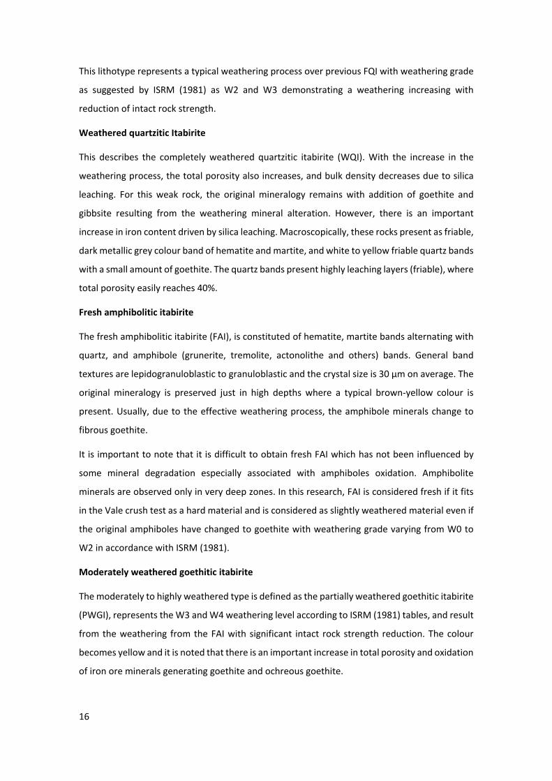
16
This lithotype represents a typical weathering process over previous FQI with weathering grade
as suggested by ISRM (1981) as W2 and W3 demonstrating a weathering increasing with
reduction of intact rock strength.
Weathered quartzitic Itabirite
This describes the completely weathered quartzitic itabirite (WQI). With the increase in the
weathering process, the total porosity also increases, and bulk density decreases due to silica
leaching. For this weak rock, the original mineralogy remains with addition of goethite and
gibbsite resulting from the weathering mineral alteration. However, there is an important
increase in iron content driven by silica leaching. Macroscopically, these rocks present as friable,
dark metallic grey colour band of hematite and martite, and white to yellow friable quartz bands
with a small amount of goethite. The quartz bands present highly leaching layers (friable), where
total porosity easily reaches 40%.
Fresh amphibolitic itabirite
The fresh amphibolitic itabirite (FAI), is constituted of hematite, martite bands alternating with
quartz, and amphibole (grunerite, tremolite, actonolithe and others) bands. General band
textures are lepidogranuloblastic to granuloblastic and the crystal size is 30 µm on average. The
original mineralogy is preserved just in high depths where a typical brown-yellow colour is
present. Usually, due to the effective weathering process, the amphibole minerals change to
fibrous goethite.
It is important to note that it is difficult to obtain fresh FAI which has not been influenced by
some mineral degradation especially associated with amphiboles oxidation. Amphibolite
minerals are observed only in very deep zones. In this research, FAI is considered fresh if it fits
in the Vale crush test as a hard material and is considered as slightly weathered material even if
the original amphiboles have changed to goethite with weathering grade varying from W0 to
W2 in accordance with ISRM (1981).
Moderately weathered goethitic itabirite
The moderately to highly weathered type is defined as the partially weathered goethitic itabirite
(PWGI), represents the W3 and W4 weathering level according to ISRM (1981) tables, and result
from the weathering from the FAI with significant intact rock strength reduction. The colour
becomes yellow and it is noted that there is an important increase in total porosity and oxidation
of iron ore minerals generating goethite and ochreous goethite.
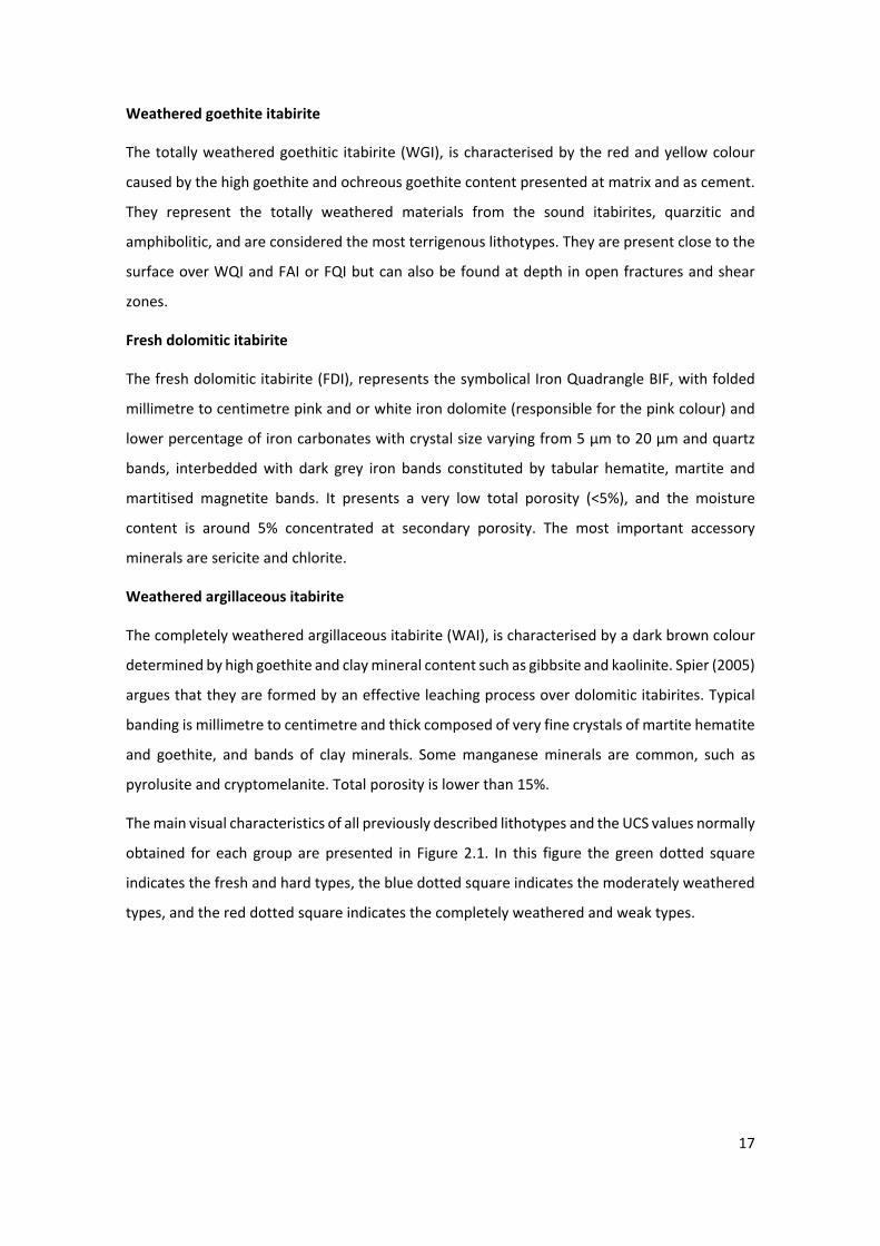
17
Weathered goethite itabirite
The totally weathered goethitic itabirite (WGI), is characterised by the red and yellow colour
caused by the high goethite and ochreous goethite content presented at matrix and as cement.
They represent the totally weathered materials from the sound itabirites, quarzitic and
amphibolitic, and are considered the most terrigenous lithotypes. They are present close to the
surface over WQI and FAI or FQI but can also be found at depth in open fractures and shear
zones.
Fresh dolomitic itabirite
The fresh dolomitic itabirite (FDI), represents the symbolical Iron Quadrangle BIF, with folded
millimetre to centimetre pink and or white iron dolomite (responsible for the pink colour) and
lower percentage of iron carbonates with crystal size varying from 5 µm to 20 µm and quartz
bands, interbedded with dark grey iron bands constituted by tabular hematite, martite and
martitised magnetite bands. It presents a very low total porosity (<5%), and the moisture
content is around 5% concentrated at secondary porosity. The most important accessory
minerals are sericite and chlorite.
Weathered argillaceous itabirite
The completely weathered argillaceous itabirite (WAI), is characterised by a dark brown colour
determined by high goethite and clay mineral content such as gibbsite and kaolinite. Spier (2005)
argues that they are formed by an effective leaching process over dolomitic itabirites. Typical
banding is millimetre to centimetre and thick composed of very fine crystals of martite hematite
and goethite, and bands of clay minerals. Some manganese minerals are common, such as
pyrolusite and cryptomelanite. Total porosity is lower than 15%.
The main visual characteristics of all previously described lithotypes and the UCS values normally
obtained for each group are presented in Figure 2.1. In this figure the green dotted square
indicates the fresh and hard types, the blue dotted square indicates the moderately weathered
types, and the red dotted square indicates the completely weathered and weak types.
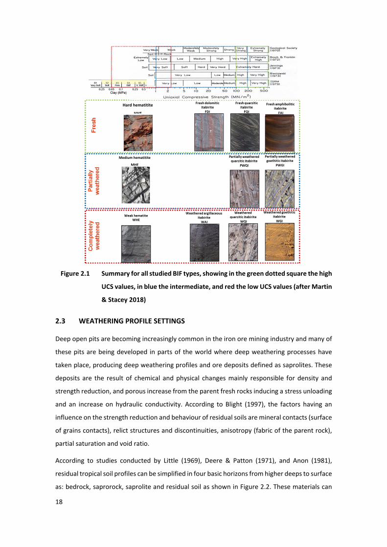
18
3 Figure 2.1 Summary for all studied BIF types, showing in the green dotted square the high
UCS values, in blue the intermediate, and red the low UCS values (after Martin
& Stacey 2018)
2.3 WEATHERING PROFILE SETTINGS
Deep open pits are becoming increasingly common in the iron ore mining industry and many of
these pits are being developed in parts of the world where deep weathering processes have
taken place, producing deep weathering profiles and ore deposits defined as saprolites. These
deposits are the result of chemical and physical changes mainly responsible for density and
strength reduction, and porous increase from the parent fresh rocks inducing a stress unloading
and an increase on hydraulic conductivity. According to Blight (1997), the factors having an
influence on the strength reduction and behaviour of residual soils are mineral contacts (surface
of grains contacts), relict structures and discontinuities, anisotropy (fabric of the parent rock),
partial saturation and void ratio.
According to studies conducted by Little (1969), Deere & Patton (1971), and Anon (1981),
residual tropical soil profiles can be simplified in four basic horizons from higher deeps to surface
as: bedrock, saprorock, saprolite and residual soil as shown in Figure 2.2. These materials can
Hard hematitite
HHE
Medium hematitite
MHE
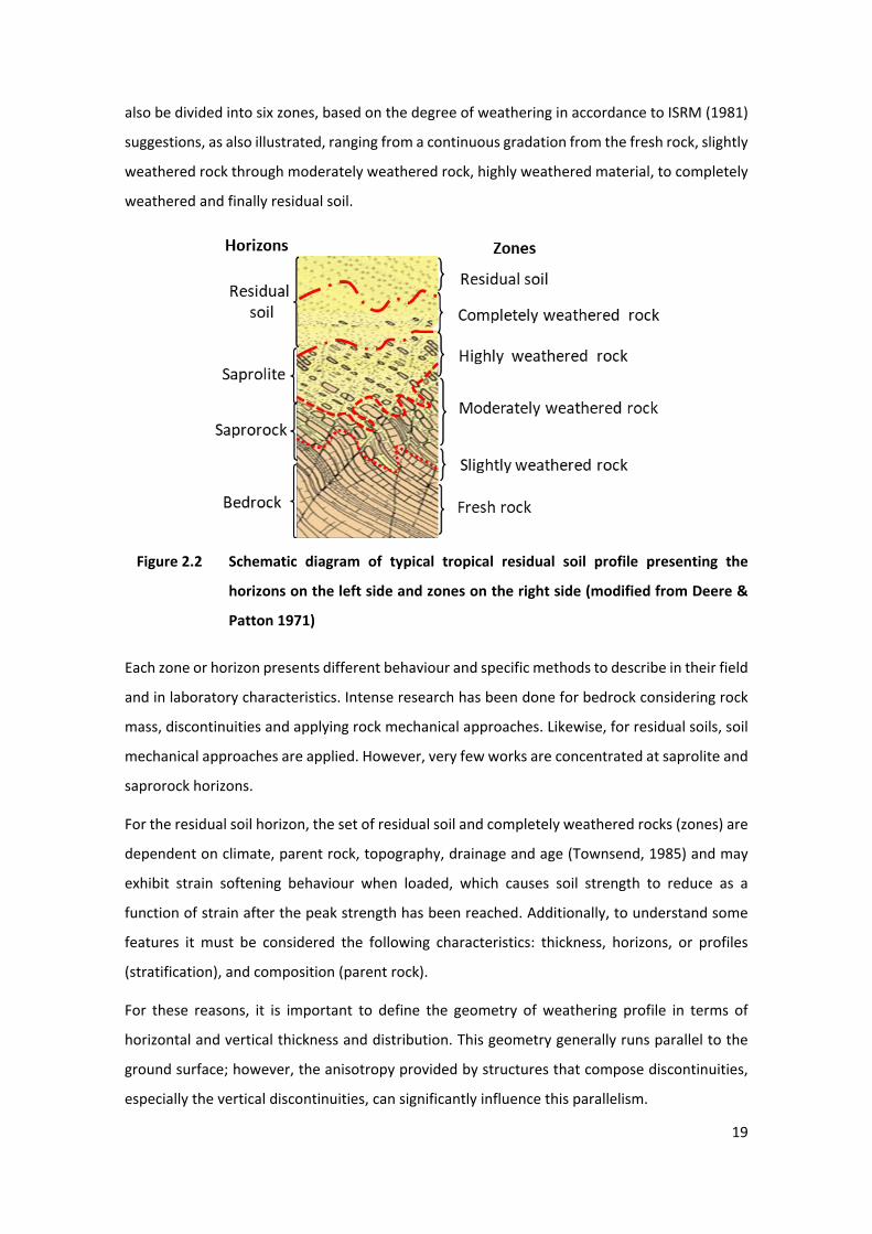
19
also be divided into six zones, based on the degree of weathering in accordance to ISRM (1981)
suggestions, as also illustrated, ranging from a continuous gradation from the fresh rock, slightly
weathered rock through moderately weathered rock, highly weathered material, to completely
weathered and finally residual soil.
4 Figure 2.2 Schematic diagram of typical tropical residual soil profile presenting the
horizons on the left side and zones on the right side (modified from Deere &
Patton 1971)
Each zone or horizon presents different behaviour and specific methods to describe in their field
and in laboratory characteristics. Intense research has been done for bedrock considering rock
mass, discontinuities and applying rock mechanical approaches. Likewise, for residual soils, soil
mechanical approaches are applied. However, very few works are concentrated at saprolite and
saprorock horizons.
For the residual soil horizon, the set of residual soil and completely weathered rocks (zones) are
dependent on climate, parent rock, topography, drainage and age (Townsend, 1985) and may
exhibit strain softening behaviour when loaded, which causes soil strength to reduce as a
function of strain after the peak strength has been reached. Additionally, to understand some
features it must be considered the following characteristics: thickness, horizons, or profiles
(stratification), and composition (parent rock).
For these reasons, it is important to define the geometry of weathering profile in terms of
horizontal and vertical thickness and distribution. This geometry generally runs parallel to the
ground surface; however, the anisotropy provided by structures that compose discontinuities,
especially the vertical discontinuities, can significantly influence this parallelism.
20
According to Lao (2013) various attempts have been made since Vargas (1953) to devise systems
for the description or classification of a completely weathered profile. A number of studies have
been carried out by researchers like Little (1969), Fookes et al. (1971), Fookes (1997), Dearman
et al. (1978), Irfan & Dearman (1978), and Anon (1981) to investigate the weathering profiles for
a descriptive degree of weathering.
Recently, with an increase in the interest in weak rock lithologies, a considerable amount of
research has been done to investigate the behaviour of completely to highly weathered rocks
mainly for mining operations, such as the recent guidelines published by Martin & Stacey (2017)
that provide a residual soil (soil-like rock) overview.
Evaluating BIF weathering profiles, due to the effectivity of the weathering process in tropical
climates induced by high pluviometry index and the topography featured, the BIF weathering
profile can often extend for more than 200 m and can reach over 400 m in depth. In addition,
the plateau morphology, syncline and anticline geological configuration and the presence of a
favourable structural control, defined by the high banding angles and extensional fractures, can
facilitate the superficial and ground water penetration and circulation, increasing the
weathering profile even more.
Weathering as a continuum and multiple conditioning processes generates a range of different
materials for each compositional BIF; from fresh to completely weathered rock. This weathering
profile presents specific and complex characteristics and boundaries between different
weathered horizons and zones.
Studies by Morris (2002 and 2002a) and Taylor et al. (2001) argue that the supergene process
can reduce the thickness of the BIF bodies by 32% to 40%, and increase the total porosity from
6% to 30%, as described by Mourão (2007). Based on that, weathering can produce an effective
softening from the leaching, and the remaining iron bands present a high total porosity, that
could be cemented by secondary iron oxides (recrystallised hematite or goethite). At more
evolved profiles, the resulting material presents weak strength, and iron enrichment promotes
an increase in bulk density due to iron minerals reconcentration. But in some week materials,
the iron oxides work as cement, improving the strength.
Additionally, studies by Ramanaidou (1989 and 2009), Ribeiro & Carvalho (2002), and Ribeiro
(2003) suggest that during the first leaching processes there have been no volumetric changes
and no quartz to goethite substitution. Progressively, the volumetric changes start to leach the
gangues minerals (more effective on dolomites, but also in quartz bands) and replace quartz to
21
goethite. This porosity could be completely cemented by goethite or iron hydroxide in superficial
levels, creating a metric hard crust called canga.
As presented by Spier et al. (2003), the superficial water is the main physical and chemical agent
responsible for effective dissolution and leaching of carbonates and siliceous minerals, and for
oxidation and hydration of iron-based minerals.
2.3.1 Failure criteria evaluation for the BIF’s weathering profiles
In the Iron Quadrangle iron ore mines, due to the predominance of weak rocks and soil material,
the Mohr–Coulomb failure criterion (MC) has often been used to define the strength parameters
required for slope stability analyses, based on direct shear and triaxial shear tests. For soil
materials, the Mohr–Coulomb criterion is the simplest and most widely used constitutive model
for determining the normal and shear stresses at failure on a loaded friction material. Bai et al.
(2010) argue that MC has been widely used in rock and soil mechanics and has good resolution
for materials that fail in the elastic range and under low strain plasticity.
However, with increasing quantities of hard rocks in deeper mines it has become necessary to
perform specific tests for these materials and, due to the popularity of the Hoek–Brown failure
criterion (HB), the unconfined compression test (UCS) has become the most important rock
strength test applicable for hard rocks. In the absence of a suitable number of these tests,
geomechanical field classification and empirical correlations with petrophysical characteristics
were used to provide input for slope stability analyses.
In Barton & Quadros (2015) it is indicated that the HB was initially proposed for the
determination of intact rock strength and rock mass strength under isotropic conditions.
Nevertheless, in recent years, with some adjustments, this criterion has been also used for the
determination of the anisotropic strengths of rocks. To use this criterion for prediction of
strength in anisotropic, intact rocks, a careful definition of the input parameters (uniaxial
compressive strength, ‘σci’, material constants ‘mi’ and ‘s’) is necessary. Moreover, the
determination of minimum and maximum intact rock strength variation due to rock anisotropy
is important in the selection of strength values for the rocks.
According to Saiang et al. (2014) there are fundamental differences between the two models or
criteria that are rather poorly understood or less well appreciated. First and foremost is the fact
that MC alone is a classic constitutive model, while HB is a failure criterion. This means that the
HB model cannot generally relate stress and strain in the same general way as the MC model.
For instance, MC is not suitable for more bright materials with tensile strength and implies a
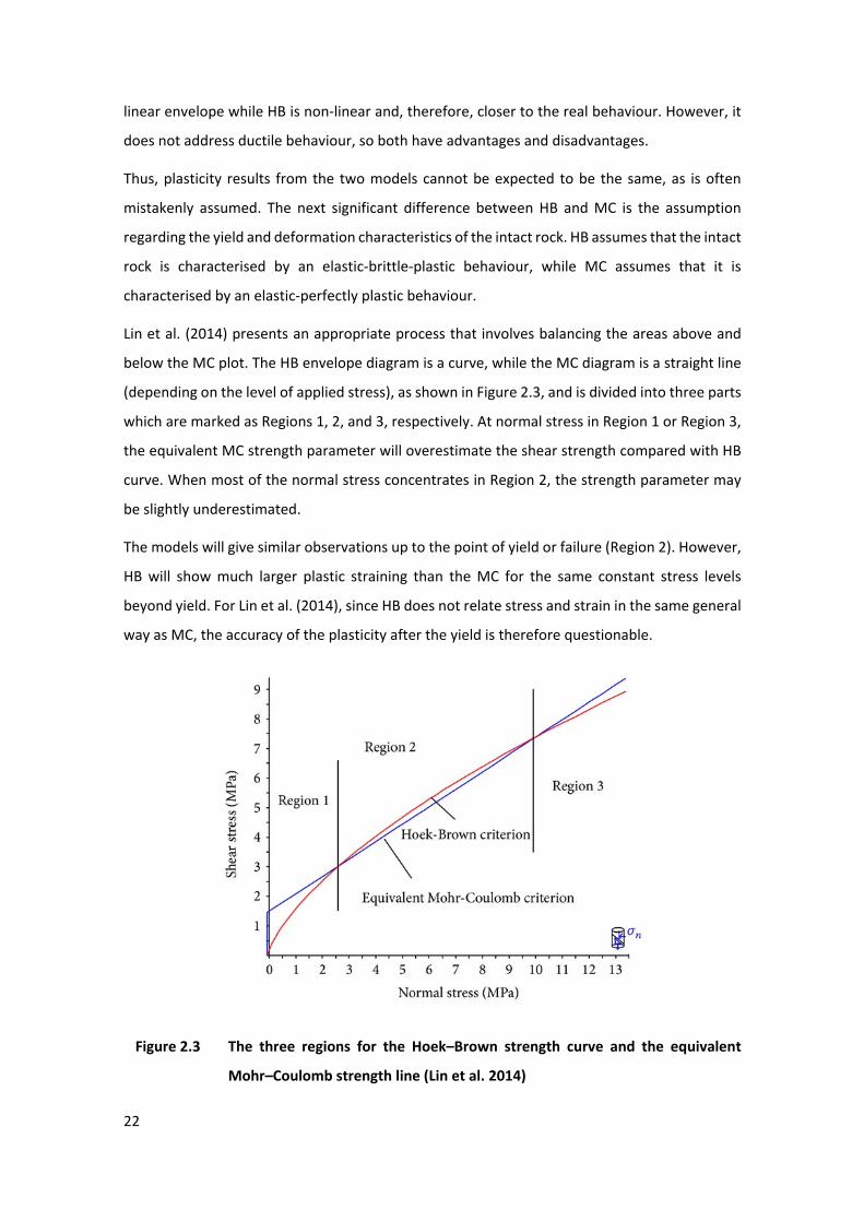
22
linear envelope while HB is non-linear and, therefore, closer to the real behaviour. However, it
does not address ductile behaviour, so both have advantages and disadvantages.
Thus, plasticity results from the two models cannot be expected to be the same, as is often
mistakenly assumed. The next significant difference between HB and MC is the assumption
regarding the yield and deformation characteristics of the intact rock. HB assumes that the intact
rock is characterised by an elastic-brittle-plastic behaviour, while MC assumes that it is
characterised by an elastic-perfectly plastic behaviour.
Lin et al. (2014) presents an appropriate process that involves balancing the areas above and
below the MC plot. The HB envelope diagram is a curve, while the MC diagram is a straight line
(depending on the level of applied stress), as shown in Figure 2.3, and is divided into three parts
which are marked as Regions 1, 2, and 3, respectively. At normal stress in Region 1 or Region 3,
the equivalent MC strength parameter will overestimate the shear strength compared with HB
curve. When most of the normal stress concentrates in Region 2, the strength parameter may
be slightly underestimated.
The models will give similar observations up to the point of yield or failure (Region 2). However,
HB will show much larger plastic straining than the MC for the same constant stress levels
beyond yield. For Lin et al. (2014), since HB does not relate stress and strain in the same general
way as MC, the accuracy of the plasticity after the yield is therefore questionable.
5 Figure 2.3 The three regions for the Hoek–Brown strength curve and the equivalent
Mohr–Coulomb strength line (Lin et al. 2014)
23
The use of MC failure envelope is established for weak completely weathered types and
laboratory test results have been used to define the intact rock strength as well as the shear
stress, as presented in Martin & Stacey (2018). For hard BIF, the HB strength curve is more
appropriate for brittle intact rock observed in these types. However, for moderately weathered
ones, the best criterion must be carefully evaluated as these rocks are a mixture of material that
exhibit soil and/or rock strength characteristics.
2.3.2 BIF weathering profile determination and implications for slope stability
For iron ore mines, the deep weathering profiles can present a mix of fresh, partially weathered,
and completely weathered material. The use of classical rock or soil mechanics must be carefully
applied to not under- or over-estimate geomechanical behaviour or misunderstand failure
mechanisms.
In shallow mines, the approach to dealing with weak rocks and slope design has largely been
based on adopting soil mechanics principles and past experiences. However, recent slope
failures and studies by Innocentini (2003), Costa (2009) and Sá (2010) suggest that some failure
mechanisms have specific characteristics for weak leached materials, and that the application
of classical soil mechanics principles does not enable failure mechanisms to be fully understood,
while rock mechanics concepts are also not fully applicable.
In those rocks, shallow, shear failures at the batter or multi batter scale are the most common
failure mechanisms. Large-scale slope failures are rare and more complex, composed of
translational and planar surfaces, the last ones controlled by unfavourable anisotropic planes
with reduced shear strength. Further, secondary influences such as high stress concentrations
at the toe of slopes, water content and discontinuities may also act as important contributing
factors.
The current approach used to undertake slope stability analysis in these types of weak rocks is
based on limit equilibrium analysis using the Mohr–Coulomb shear strength criterion and, in
some special cases, supported by numerical models. The shear strength and elastic parameters
for these designs are normally based on a limited number of intact rock laboratory tests which
are mainly saturated triaxial and direct shear test and supported by adapted rock mass
classifications. While this approach has been mostly successful, it would appear from experience
that they are conservative. Despite that, there have been examples of large slope failures not
captured by these design approaches that have had significant negative impacts on mine
production.
24
The situation is particularly challenging when considering the stratigraphic position and/or
tectonic settings of the weak rocks that are very often located at the toe of high slopes (more
than 400 m depth), where the stress is concentrated. To address this issue, Vale geotechnical
engineers have historically designed a buttress of ore to be left at the toe of the wall, resulting
in a loss of ore reserves, as suggested in Costa et al. (2009).
In addition to classical soil mechanics laboratory testing, to support these materials’ complete
characterisation, other parameters are evaluated such as: total porosity, bulk density, particle
size distribution curves, mineralogy, and anisotropy have been considered in relation to slope
stability behaviour. Describing and correlating these parameters remains a key challenge to the
authors due to the difficulties associated with sample acquisition, testing, scale effect and
sample representativeness.
An important characteristic generally neglected for BIF due to the high permeability and low
plasticity observed on those materials is the matric suction effect on slope stability. However, a
minor presence of clay minerals can influence the slope stability, as presented by Lu and Likos
(2004) which argue that the matric suction contributes to the cohesion and increases the shear
strength of unsaturated soils. Studies by Grgic et al. (2005) on iron formations suggested that an
improvement on the strength and cohesion of partially saturated oolithic iron ore can occur due
to the negative porewater pressure effects.
It has been noted from work outside the mining industry that the shear strength of a soil with
negative porewater pressure can increase the stability of slopes, especially those having shallow
but steep surfaces as supported by Fredlund et al. (1978). So far, matric suction effects have not
been considered in Vale open pit slope stability evaluations where effective stress parameters
are obtained by conventional saturated laboratory testing. This approach seems to be adequate
for high pluviometric index areas where long-term slope stability is required. However, it tends
to be too conservative when applied to the design of short-term slopes above the water level.
The use of unsaturated soil mechanics is therefore necessary to correct the balance between
safety and economical slope designing.
In addition, for Iron Quadrangle mines, studies by Soares (2008) and Ventura & Bacellar (2012)
for country rocks showed the importance of suction effects on iron ore mines’ slope stability
analysis, especially for shallow surfaces.
Contrasting, from fresh and hard BIF, for future proposed deepest open pit mines, there will be
an increase in the percentage of hard and fresh rock exposed, which poses new challenges to
the geotechnical team. They may need to develop slope design criteria and evaluate possible
25
failure mechanisms in hard rock by using classical rock mechanics principles, breaking some
paradigms established over recent decades operating mainly in weak rocks.
For these hard rocks, it is crucial to ensure a good evaluation of intact rock strength, as well as
geotechnical characteristics of discontinuities to understand slope deformation behaviour for
quite a complex arrangement of different rock mass strength materials.
It is also important to determine geotechnical parameters for partially weathered rocks
(a mixture of hard and weak rocks) and to develop a method to better define and map the
boundaries along the weathering continuum.
2.4 ROCK MECHANICS APPROACHES FOR FRESH TO MODERATELY WEATHERED BIF
Slope stability analysis for material with high-value of intact rock strength (fresh to slightly
weathered BIF) is controlled by the discontinuities shear strength and rock mass strength. For
partially weathered itabirites, the reduction in intact rock strength imposed by the weathering
can change this setting, and slope stability analyses are controlled by intact rock strength and
possible associated heterogeneity. It remains unknown where in the weathering horizon of the
fresh rock (bedrock) is reduced to saprorock, and to such an extent that it reaches these strength
reductions, changing the slope stability control.
For the bedrock, UCS testing is largely used, as a direct parameter, to determine rock strength
and indirect tests also applied as: point load test (PLT), Schmidt hammer test and tactile visual
or qualitative estimation based on characteristic tables and geomechanical classifications.
Many past experiences of geomechanical classification have been proposed for iron ore mines
and associated country rocks, even with some attempts from Vale geotechnical and consultant
teams. These experiences suggest that in many cases the use of geomechanical classification has
proven to be more than adequate and reliable to correlate with intact rock strength based on
minimum UCS test results. However, these simple estimation methods must have an adequate
laboratory test calibration and field strength estimation to fully meet complex slope stability
analysis.
The establishment of a standard characteristic table and rock mass classification for the Iron
Quadrangle’s BIF has been proposed by several authors (Zenobio, 2000; Zenobio & Zuquete,
2004; Castro et al., 2013; and Araujo et al., 2014). These authors generally adapt classical
geomechanical classifications using, for example, specific field procedures and tests, calibrated
with laboratory tests results.
26
For fresh rock in Vale mines, the adapted strength field characterisation tables, crush tests and
a limited number of intact mass UCS tests have been used to determine the intact rock strength
and guide slope stability evaluation. Although this approach has been satisfactory, the increase
of fresh rock in deeper mines demands a higher level of confidence and a more reliable
database.
This approach is largely used in different rock types, and historically, index proprieties
interrelationships with rock strength have been established worldwide for several rock types.
Gupta and Rao (1998 and 2001) and Irfan & Dearman (1978) mainly focused on granitic rocks
established correlations between the physical proprieties of the rocks to the weathering process
for geotechnical evaluations.
Specifically, for BIF a similar access was established by Aylmer et al. (1978) evaluating the bulk
density, iron grade and total porosity for Mount Tom Price iron ore mine and concluded that the
iron grade and the bulk density have a good correlation; however, the accuracy was largely
affected by high and variable total porosity.
Also, according to Box and Reid (1976) for iron ore formation from Cockatoo Island, true specific
gravity could be expressed as a function of iron content; however, due to the complexity and
multiple factors the same influence could not be established for total porosity. Thomson (1963)
concluded that for iron ore samples from Australia, a theoretical hematite-quartz curve can be
used for bulk density definition and can present an approximate iron content calculation. For
Sishen South iron deposits, Nel (2007) established that total porosity is directly correlated to the
dry and bulk density providing a reliable calculation index. These works are based on the same
correlation and presented similar findings for different worldwide BIF deposits.
In Brazil, studies of Ribeiro (2014), Santos et al. (2005) and Santos (2007) evaluating the
association between bulk density and iron content for Vales iron mines, concluded that there is
a linear positive correlation between iron content and bulk density. They also presented that
weathering process has an important influence on this correlation and iron content dispersion
is imposed by total porosity. The most significant type of total porosity for slope stability and
engineering applications is the interconnected porosity or effective porosity, due to its relevance
on strength and capacity of transmitting fluids through connected pores. In rock engineering
porosity is an important physical parameter for evaluation of water storage capacity,
identification of weathering profiles and correlations with strength.
However, as proposed by Saroglou et al. (2004), mineral composition, fabric, grain size, degree
of weathering, and anisotropy also influence the strength and deformation of intact rocks.
27
The correlation between UCS and physical properties such as bulk density (𝜌𝜌b), P wave velocity
and elastic properties has been largely used. However, a smaller number of publications
explored the influence of rock banding on strength characteristics of BIF. The study from
Gonçalves et al. (2012), concludes that at slower strain rate the matrix-controlled rheology takes
over and strength of BIF is not dependent on fabric anisotropy or on iron oxide content. The
banded sample becomes as weak as pure and homogeneous hematite aggregate. It also
indicates that iron oxide content and strain rate are controlling factors on BIF.
Another approach used to in this thesis is the evaluation of the dynamic modulus, using
compressional (P) and shear (S) wave velocity that has been used by many authors as a
non-destructive method for physical characterisation of intact rock strength. As shown by Turk
& Dearman, (1986), and Karpuz & Pasamehmetoglu (1997) such experiments are used for
determination of rock weathering degree, fluid saturation, presence of discontinuities and as
input data in geotechnical models and rock engineering applications. P and S wave velocities
have important correlation with other physical and strength properties of rocks such as total
porosity, bulk density, and UCS test results.
Dynamic elastic parameters of rock are well described parameters obtained throughout
empirical relationship among P and S wave velocities and 𝜌𝜌b of samples described by elasticity
theory. From theoretical relationships, P and S wave velocities are also used to calculate dynamic
elastic modulus (Edyn), dynamic shear modulus (Gdyn), dynamic bulk modulus (Kdyn) and dynamic
Poison’s ratio (νdyn), according to the equations presented by Bourbié et al. (1987), Sheriff
(1991), and Soares (1992). The application of these properties is limited to its relationship with
the static deformation modulus. This relationship can only be verified by empirical relations once
there is a huge variation among different rock types. Additionally, dynamic laboratory
measurements (acoustic) can be used to help calibrate the mechanical properties calculated
from the petrophysical model. In the absence of laboratory data, most of these results must fit
within known ranges, depending on lithology (Crain & Holgate 2014). After proposing correct
relationships, dynamic elastic modulus can be used as crucial information for geomechanical
models in mining applications such as slope stability and slope monitoring.
2.5 SOIL MECHANICS APPROACHES FOR COMPLETELY WEATHERED BIF
Soil lithotypes in mining operations are evaluated based on soil mechanics approaches and the
shear strength is obtained performing saturated soil laboratory tests due to the test velocity and
the possibility to determine effective and total strength and obtain MC parameters normally
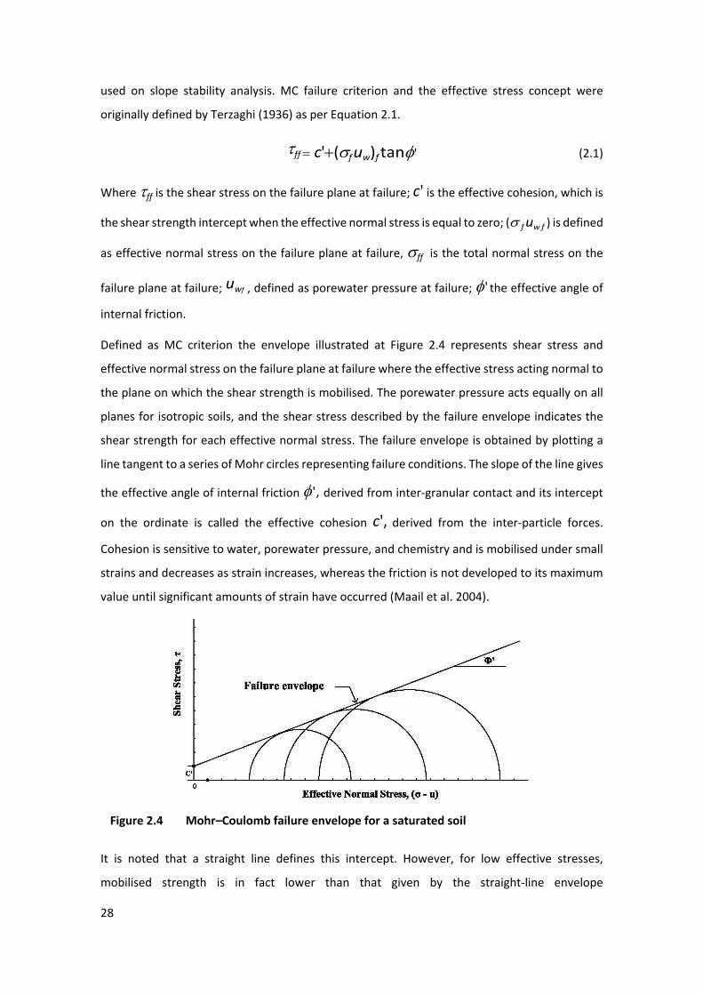
28
used on slope stability analysis. MC failure criterion and the effective stress concept were
originally defined by Terzaghi (1936) as per Equation 2.1.
τff = c'+(σf uw)f tanφ' 1(2.1)
Where τff is the shear stress on the failure plane at failure; c' is the effective cohesion, which is
the shear strength intercept when the effective normal stress is equal to zero; (σ f uw f ) is defined
as effective normal stress on the failure plane at failure, σff is the total normal stress on the
failure plane at failure; uwf , defined as porewater pressure at failure; φ' the effective angle of
internal friction.
Defined as MC criterion the envelope illustrated at Figure 2.4 represents shear stress and
effective normal stress on the failure plane at failure where the effective stress acting normal to
the plane on which the shear strength is mobilised. The porewater pressure acts equally on all
planes for isotropic soils, and the shear stress described by the failure envelope indicates the
shear strength for each effective normal stress. The failure envelope is obtained by plotting a
line tangent to a series of Mohr circles representing failure conditions. The slope of the line gives
the effective angle of internal friction φ', derived from inter-granular contact and its intercept
on the ordinate is called the effective cohesion c', derived from the inter-particle forces.
Cohesion is sensitive to water, porewater pressure, and chemistry and is mobilised under small
strains and decreases as strain increases, whereas the friction is not developed to its maximum
value until significant amounts of strain have occurred (Maail et al. 2004).
6 Figure 2.4 Mohr–Coulomb failure envelope for a saturated soil
It is noted that a straight line defines this intercept. However, for low effective stresses,
mobilised strength is in fact lower than that given by the straight-line envelope
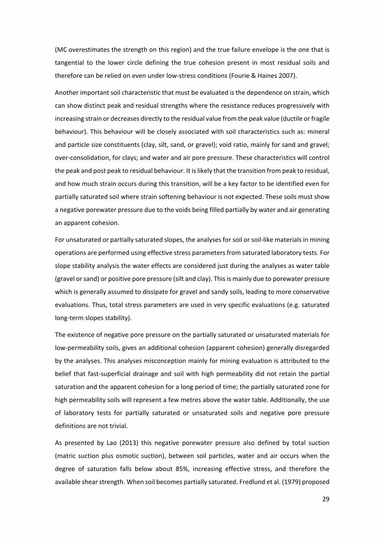
29
(MC overestimates the strength on this region) and the true failure envelope is the one that is
tangential to the lower circle defining the true cohesion present in most residual soils and
therefore can be relied on even under low-stress conditions (Fourie & Haines 2007).
Another important soil characteristic that must be evaluated is the dependence on strain, which
can show distinct peak and residual strengths where the resistance reduces progressively with
increasing strain or decreases directly to the residual value from the peak value (ductile or fragile
behaviour). This behaviour will be closely associated with soil characteristics such as: mineral
and particle size constituents (clay, silt, sand, or gravel); void ratio, mainly for sand and gravel;
over-consolidation, for clays; and water and air pore pressure. These characteristics will control
the peak and post peak to residual behaviour. It is likely that the transition from peak to residual,
and how much strain occurs during this transition, will be a key factor to be identified even for
partially saturated soil where strain softening behaviour is not expected. These soils must show
a negative porewater pressure due to the voids being filled partially by water and air generating
an apparent cohesion.
For unsaturated or partially saturated slopes, the analyses for soil or soil-like materials in mining
operations are performed using effective stress parameters from saturated laboratory tests. For
slope stability analysis the water effects are considered just during the analyses as water table
(gravel or sand) or positive pore pressure (silt and clay). This is mainly due to porewater pressure
which is generally assumed to dissipate for gravel and sandy soils, leading to more conservative
evaluations. Thus, total stress parameters are used in very specific evaluations (e.g. saturated
long-term slopes stability).
The existence of negative pore pressure on the partially saturated or unsaturated materials for
low-permeability soils, gives an additional cohesion (apparent cohesion) generally disregarded
by the analyses. This analyses misconception mainly for mining evaluation is attributed to the
belief that fast-superficial drainage and soil with high permeability did not retain the partial
saturation and the apparent cohesion for a long period of time; the partially saturated zone for
high permeability soils will represent a few metres above the water table. Additionally, the use
of laboratory tests for partially saturated or unsaturated soils and negative pore pressure
definitions are not trivial.
As presented by Lao (2013) this negative porewater pressure also defined by total suction
(matric suction plus osmotic suction), between soil particles, water and air occurs when the
degree of saturation falls below about 85%, increasing effective stress, and therefore the
available shear strength. When soil becomes partially saturated. Fredlund et al. (1979) proposed
30
Equation 2.2 for unsaturated soil in which two independent stress state variables, the net
normal stress, (σ − ua) and the matric suction, (ua− uw) are used.
τf= c'+(ua − uw )tanφ b + (σ − u )tanφ' 2(2.2)
Where τf is the shear strength, c' is effective cohesion intercept, ua is pore air pressure, uw is
porewater pressure, φ b is the angle of cohesion intercept increase with increasing suction, σ is
the total stress and φ ' is the effective angle of shear resistance. This shear strength equation
defines a planar surface called the extended Mohr–Coulomb failure envelope, as shown in
Figure 2.5 (Gan et al. 1988).
7 Figure 2.5 Extended Mohr–Coulomb failure envelope for unsaturated soils (Gan &
Fredlund et al. 1988)
Positive or zero pore pressures result in matric suction effects which can explain why some soils’
slopes are stable even with angles that are steeper than would be predicted by Equation 2.1,
and why many falls happened during heavy rainfall, even when a rise in the watertable does not
occur. These falls occur with an increase of degree of saturation without necessarily reaching
100% resulting only in a decrease or loss of the additional strength component generated by
matric suction.
Rahardjo et al. (2014) developed an axis translation technique from apparatus capable of
controlling and measuring pore air and porewater pressure enabling the measurement of shear
strength for unsaturated condition, plotting, and interpreting pore pressure effects on total
material strength at an extended three-dimensional MC envelope. Procedures and apparatus
31
used in this technique are described in Fredlund at al. (2012). Using this technique according to
Fredlund et al. (2014) the failure envelope intersects shear strength versus matric suction planes
at a total cohesion, and when this can be obtained for different matric suction, values are
defined an extend MC failure envelope giving φ b angle. This angle was defined by Lee et al. (2005)
as equal to φ' for matric suction less than or equal to the air entry value (AEV), or where φ b is
lower than φ' for matric suction and higher than AEV.
To define the shear strength equation for unsaturated soils one possible approach is to use
estimation equations based on saturated shear strength parameters and soil classification
proprieties as supported by Vanapalli et al. (1996), Fredlund et al. (1996), Oberg & Allfors (1997),
Khalili & Khabbaz (1998), Bao et al. (1998) and Goh et al. (2010). Fitting equations were
described by Fredlund et al. (1978 and 1996).

32
33
CHAPTER 3. METHODOLOGY
The main aims of this research will be discussed using the following three different approaches:
• Use of Vale’s geological and geotechnical database to evaluate and correlate
geomechanical properties of the BIF to understand intact rock strength variation in
response to the weathering.
• Development of a laboratory testing programme, focusing on intact rock
characteristics to determine petrophysical, intact rock strength and elastic parameters
using different approaches for hard and weak rocks in order to complement
information not available or insufficient on the Vale´s database.
• Petrographic thin sections analysis to assess the rock microcharacteristics and its
correlation to weathering changes. Ultimately, this approach will correlate
microgeological with macrogeological and geotechnical features.
With these approaches, it is expected to best correlate weathering profile horizons and zones
with strength and elastic parameters, thus promoting a more complete and comprehensive
understanding of geotechnical behaviour of rock weathering variables and its influence at open
pit excavation. From that, pit design can be optimised so that maximum ore can be recovered,
with the required level of stability and associated level of safety.
In order to achieve proposed objectives, a three-phase methodology was used.
• Phase one: Carried out during the years 2013 and 2014, a field investigation was
undertaken, and several samples collected from outcrops and from core drills for all
BIF lithotypes. Geological and geotechnical information were logged, based on ISRM
(1981) suggestions, and petrophysical characteristics were described (e.g. qualitative
anisotropy and banding) to support the analysis of laboratory test results. Outcrops
and samples were photographed for additional visual information such as anisotropy
plans, banding, type of BIF and discontinuities. A literature review was also performed
and evaluated for problem statement, and evaluation of the Vale geotechnical and
geological database was also conducted.
• Phase two: Carried out during the years 2014 to 2016, focused on the description of
petrographic thin sections, to evaluate the rock mineralogy, fabric, total porosity, and
to provide information on a microscopic scale to be compared with field
macrocharacteristics described in the first stage, to provide geological and
34
geotechnical field work validation. Finally, all laboratory tests for soil and rock
materials were run in Brazilian and Australian laboratories.
• Phase three: Carried out during the years 2015 to 2021, included the evaluation of all
laboratory tests, results used and complied to determine the intact rock properties
together with the correlations with geological characteristics and other geotechnical
parameters of each lithotype obtained during the previous phases. This phase includes
data interpretation, evaluation of the results, draw conclusions and PhD dissertation
development were determined.
3.1 FIELDWORK AND SAMPLING
From the fifteen studied mines the sampling campaign covered different weathering horizons
and degree levels considering all studied BIF lithotypes and typologies. Geological and structural
information was collected, and the geotechnical information described was based on the ISRM
(1981) suggestion tables, and all samples and outcrops were photographed and used to support
the visual information for laboratory tests and physical parameter recognition (e.g. anisotropy
and banding).
Data from previous laboratory test reports available in Vale’s database and from laboratory tests
specifically performed in Brazilian and Australian laboratories were used. The use of Vale’s
previous laboratory test reports was considered just when all geological and geotechnical
information were available.
A total of 21 block samples were shipped to the petrophysical laboratory of the Campina Grande
University at Paraiba state, Brazil to test porosity, permeability, and P and S wave velocity for
fresh to moderately weathered BIF. A total of 10 block samples were shipped to Geocontrole Br
Sondagens laboratory at Nova Lima, Minas Gerais state, Brazil to perform geotechnical soil and
rock tests.
To Australia, more than 500 kg of drill cores and block samples were shipped to The Australian
Centre of Geomechanics/Department of Civil, Environmental and Mining Engineering, The
University of Western Australia and E-precision Laboratory both located in Perth, Western
Australia, for rock and soil geotechnical tests.
3.2 DATABASE CONSISTENCY APPROACHS AND DEFINITIONS
Laboratory test results were evaluated as graphs and tables to verify the correlation between
the geotechnical parameters and to define the level of correlation. From those graphs,
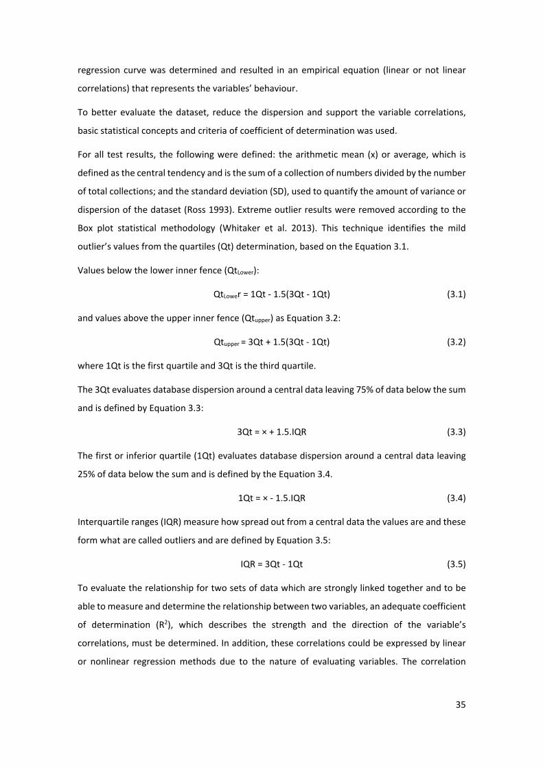
35
regression curve was determined and resulted in an empirical equation (linear or not linear
correlations) that represents the variables’ behaviour.
To better evaluate the dataset, reduce the dispersion and support the variable correlations,
basic statistical concepts and criteria of coefficient of determination was used.
For all test results, the following were defined: the arithmetic mean (x) or average, which is
defined as the central tendency and is the sum of a collection of numbers divided by the number
of total collections; and the standard deviation (SD), used to quantify the amount of variance or
dispersion of the dataset (Ross 1993). Extreme outlier results were removed according to the
Box plot statistical methodology (Whitaker et al. 2013). This technique identifies the mild
outlier’s values from the quartiles (Qt) determination, based on the Equation 3.1.
Values below the lower inner fence (QtLower):
QtLower = 1Qt - 1.5(3Qt - 1Qt) (3.1)
and values above the upper inner fence (Qtupper) as Equation 3.2:
Qtupper = 3Qt + 1.5(3Qt - 1Qt) (3.2)
where 1Qt is the first quartile and 3Qt is the third quartile.
The 3Qt evaluates database dispersion around a central data leaving 75% of data below the sum
and is defined by Equation 3.3:
3Qt = × + 1.5.IQR (3.3)
The first or inferior quartile (1Qt) evaluates database dispersion around a central data leaving
25% of data below the sum and is defined by the Equation 3.4.
1Qt = × - 1.5.IQR (3.4)
Interquartile ranges (IQR) measure how spread out from a central data the values are and these
form what are called outliers and are defined by Equation 3.5:
IQR = 3Qt - 1Qt (3.5)
To evaluate the relationship for two sets of data which are strongly linked together and to be
able to measure and determine the relationship between two variables, an adequate coefficient
of determination (R2), which describes the strength and the direction of the variable’s
correlations, must be determined. In addition, these correlations could be expressed by linear
or nonlinear regression methods due to the nature of evaluating variables. The correlation
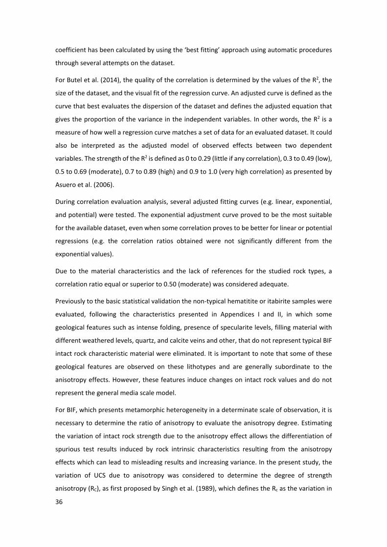
36
coefficient has been calculated by using the ‘best fitting’ approach using automatic procedures
through several attempts on the dataset.
For Butel et al. (2014), the quality of the correlation is determined by the values of the R2, the
size of the dataset, and the visual fit of the regression curve. An adjusted curve is defined as the
curve that best evaluates the dispersion of the dataset and defines the adjusted equation that
gives the proportion of the variance in the independent variables. In other words, the R2 is a
measure of how well a regression curve matches a set of data for an evaluated dataset. It could
also be interpreted as the adjusted model of observed effects between two dependent
variables. The strength of the R2 is defined as 0 to 0.29 (little if any correlation), 0.3 to 0.49 (low),
0.5 to 0.69 (moderate), 0.7 to 0.89 (high) and 0.9 to 1.0 (very high correlation) as presented by
Asuero et al. (2006).
During correlation evaluation analysis, several adjusted fitting curves (e.g. linear, exponential,
and potential) were tested. The exponential adjustment curve proved to be the most suitable
for the available dataset, even when some correlation proves to be better for linear or potential
regressions (e.g. the correlation ratios obtained were not significantly different from the
exponential values).
Due to the material characteristics and the lack of references for the studied rock types, a
correlation ratio equal or superior to 0.50 (moderate) was considered adequate.
Previously to the basic statistical validation the non-typical hematitite or itabirite samples were
evaluated, following the characteristics presented in Appendices I and II, in which some
geological features such as intense folding, presence of specularite levels, filling material with
different weathered levels, quartz, and calcite veins and other, that do not represent typical BIF
intact rock characteristic material were eliminated. It is important to note that some of these
geological features are observed on these lithotypes and are generally subordinate to the
anisotropy effects. However, these features induce changes on intact rock values and do not
represent the general media scale model.
For BIF, which presents metamorphic heterogeneity in a determinate scale of observation, it is
necessary to determine the ratio of anisotropy to evaluate the anisotropy degree. Estimating
the variation of intact rock strength due to the anisotropy effect allows the differentiation of
spurious test results induced by rock intrinsic characteristics resulting from the anisotropy
effects which can lead to misleading results and increasing variance. In the present study, the
variation of UCS due to anisotropy was considered to determine the degree of strength
anisotropy (RC), as first proposed by Singh et al. (1989), which defines the Rc as the variation in
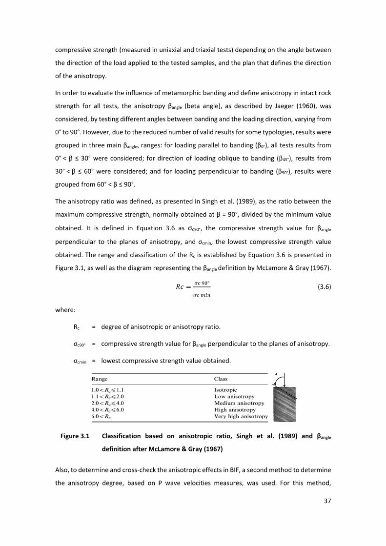
37
compressive strength (measured in uniaxial and triaxial tests) depending on the angle between
the direction of the load applied to the tested samples, and the plan that defines the direction
of the anisotropy.
In order to evaluate the influence of metamorphic banding and define anisotropy in intact rock
strength for all tests, the anisotropy βangle (beta angle), as described by Jaeger (1960), was
considered, by testing different angles between banding and the loading direction, varying from
0° to 90°. However, due to the reduced number of valid results for some typologies, results were
grouped in three main βangles ranges: for loading parallel to banding (β0°), all tests results from
0° < β ≤ 30° were considered; for direction of loading oblique to banding (β45°), results from
30° < β ≤ 60° were considered; and for loading perpendicular to banding (β90°), results were
grouped from 60° < β ≤ 90°.
The anisotropy ratio was defined, as presented in Singh et al. (1989), as the ratio between the
maximum compressive strength, normally obtained at β = 90°, divided by the minimum value
obtained. It is defined in Equation 3.6 as σc90°, the compressive strength value for βangle
perpendicular to the planes of anisotropy, and σcmin, the lowest compressive strength value
obtained. The range and classification of the Rc is established by Equation 3.6 is presented in
Figure 3.1, as well as the diagram representing the βangle definition by McLamore & Gray (1967).
𝑅𝑅𝑅𝑅 = 𝜎𝜎𝜎𝜎 90°
𝜎𝜎𝜎𝜎 𝑚𝑚𝑚𝑚𝑚𝑚 (3.6)
where:
Rc = degree of anisotropic or anisotropy ratio.
σc90° = compressive strength value for βangle perpendicular to the planes of anisotropy.
σcmin = lowest compressive strength value obtained.
8 Figure 3.1 Classification based on anisotropic ratio, Singh et al. (1989) and βangle
definition after McLamore & Gray (1967)
Also, to determine and cross-check the anisotropic effects in BIF, a second method to determine
the anisotropy degree, based on P wave velocities measures, was used. For this method,
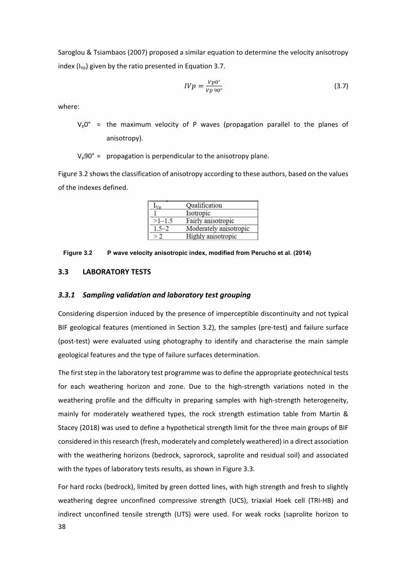
38
Saroglou & Tsiambaos (2007) proposed a similar equation to determine the velocity anisotropy
index (IVp) given by the ratio presented in Equation 3.7.
𝐼𝐼𝐼𝐼𝐼𝐼 = 𝑉𝑉𝑉𝑉0°𝑉𝑉𝑉𝑉 90°
(3.7)
where:
Vp0° = the maximum velocity of P waves (propagation parallel to the planes of
anisotropy).
Vp90° = propagation is perpendicular to the anisotropy plane.
Figure 3.2 shows the classification of anisotropy according to these authors, based on the values
of the indexes defined.
9 Figure 3.2 P wave velocity anisotropic index, modified from Perucho et al. (2014)
3.3 LABORATORY TESTS
3.3.1 Sampling validation and laboratory test grouping
Considering dispersion induced by the presence of imperceptible discontinuity and not typical
BIF geological features (mentioned in Section 3.2), the samples (pre-test) and failure surface
(post-test) were evaluated using photography to identify and characterise the main sample
geological features and the type of failure surfaces determination.
The first step in the laboratory test programme was to define the appropriate geotechnical tests
for each weathering horizon and zone. Due to the high-strength variations noted in the
weathering profile and the difficulty in preparing samples with high-strength heterogeneity,
mainly for moderately weathered types, the rock strength estimation table from Martin &
Stacey (2018) was used to define a hypothetical strength limit for the three main groups of BIF
considered in this research (fresh, moderately and completely weathered) in a direct association
with the weathering horizons (bedrock, saprorock, saprolite and residual soil) and associated
with the types of laboratory tests results, as shown in Figure 3.3.
For hard rocks (bedrock), limited by green dotted lines, with high strength and fresh to slightly
weathering degree unconfined compressive strength (UCS), triaxial Hoek cell (TRI-HB) and
indirect unconfined tensile strength (UTS) were used. For weak rocks (saprolite horizon to
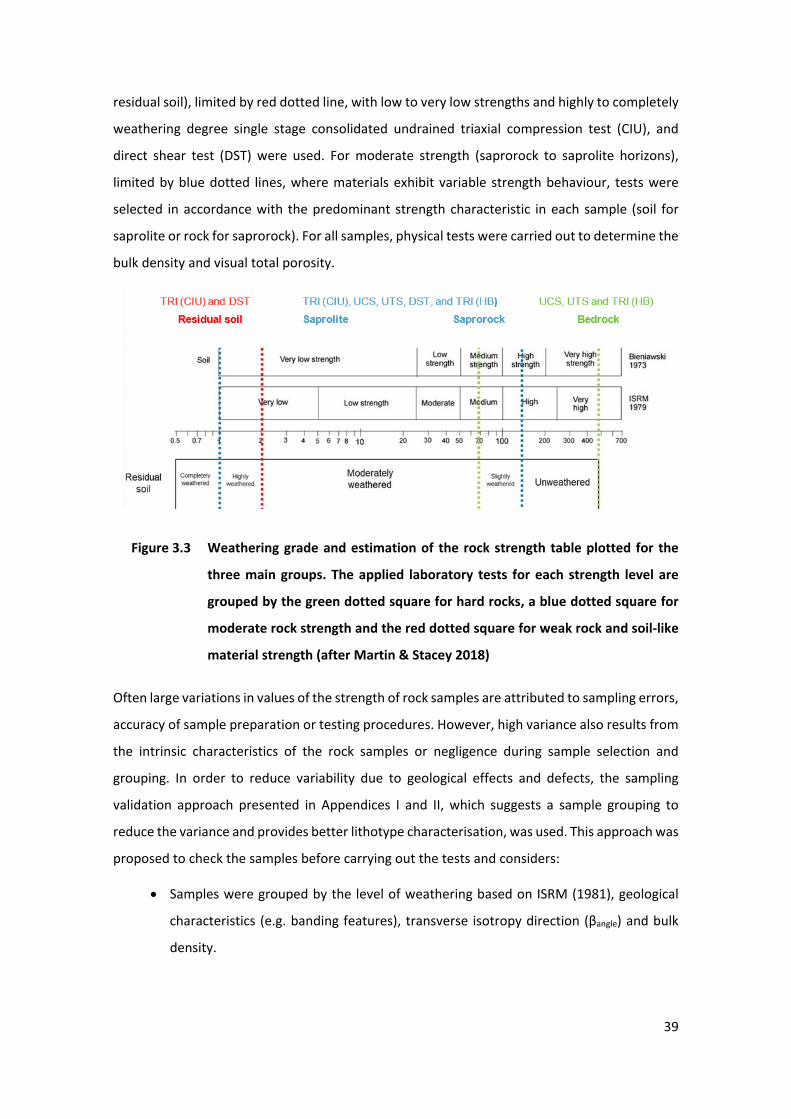
39
residual soil), limited by red dotted line, with low to very low strengths and highly to completely
weathering degree single stage consolidated undrained triaxial compression test (CIU), and
direct shear test (DST) were used. For moderate strength (saprorock to saprolite horizons),
limited by blue dotted lines, where materials exhibit variable strength behaviour, tests were
selected in accordance with the predominant strength characteristic in each sample (soil for
saprolite or rock for saprorock). For all samples, physical tests were carried out to determine the
bulk density and visual total porosity.
10 Figure 3.3 Weathering grade and estimation of the rock strength table plotted for the
three main groups. The applied laboratory tests for each strength level are
grouped by the green dotted square for hard rocks, a blue dotted square for
moderate rock strength and the red dotted square for weak rock and soil-like
material strength (after Martin & Stacey 2018)
Often large variations in values of the strength of rock samples are attributed to sampling errors,
accuracy of sample preparation or testing procedures. However, high variance also results from
the intrinsic characteristics of the rock samples or negligence during sample selection and
grouping. In order to reduce variability due to geological effects and defects, the sampling
validation approach presented in Appendices I and II, which suggests a sample grouping to
reduce the variance and provides better lithotype characterisation, was used. This approach was
proposed to check the samples before carrying out the tests and considers:
• Samples were grouped by the level of weathering based on ISRM (1981), geological
characteristics (e.g. banding features), transverse isotropy direction (βangle) and bulk
density.
40
• For fresh rocks, P wave velocity (Vp) measurements were used to discard inadequate
samples (inclusions or fractured).
• Itabirites samples that did not show typical banding were not evaluated, thereby
heterogeneity was included and evaluated, and the scale effect related to the
compositional band thickness was qualitatively evaluated.
• Extreme outlier results were removed according to the Box plot statistical
methodology, in accordance with Whitaker et al. (2013) and Ross (1993). This
technique identifies the mild outlier’s values from the quartiles (Qt) determination,
based on the criteria described in Section 3.2.
These approaches aimed to evaluate all samples and identify possible drawbacks that may
influence results increasing dispersion.
Soil and rock materials, present different geomechanical characteristics and parameters, and
are determined by different methodologies, laboratory test and standards. For this reason, they
were presented separately.
3.3.2 Rock mechanics tests
All rock laboratory test results are presented in Appendices III, IV, and V. The rock tests
performed and used in this thesis are listed and described below. All tests were undertaken in
different anisotropic directions (βangle) as presented in Section 3.2.
Unconfined compressive strength test
According to Hoek (1977), among all strength properties of rocks, the UCS is the most used
strength parameter by industry and academia. Moreover, it is a test with high variance induced
by sample preparation, imperfections or associated intrinsic characteristics such as
heterogeneities, anisotropy, no visible discontinuities, and other defects or effects. To reduce
the dispersion caused by geological features and defects, sampling validation presented in
Section 3.3.1 was applied, which suggests sample grouping by similar geological characteristics
such as banding type, bulk density, and presence of typical BIF geological features.
At the Australian laboratory, UCS tests were performed in accordance with ASTM D 2938-95
(ASTM 2002). For all tests, samples (cylindrical plugs) were obtained from original 77.8 mm
diamond drill core subsampled in 20 mm diameter with lengths varying from 40 mm to 50 mm
and prepared accordingly to ASTM D4543-01 (ASTM 2001).
41
For better axial and lateral strains, simultaneous measurements with a minimum of one and
maximum of three diametric pairs of strain gauges were used. The tests were subjected to a
constant loading rate of 7 MPa/min or 9 MPa/min. The average strain was calculated by taking
the average of all strain readings. The modulus was calculated by the moving average of mean
strain.
The Brazilian laboratory tests were performed according to ASTM D 2938-95 (ASTM 2002). The
cylindrical samples were obtained from drilling rock blocks with 76 mm diameter with lengths
varying from 110 mm to 205 mm. All samples were prepared according to ASTM D4543-01
(ASTM 2001). Double dial indicator gauges obtained the axial and lateral measurements, and
the strain was used to calculate by taking the average in each direction. It is noted that dial
indicators have presented less efficiency on strain measurement compared with the strain
gauges used in Australian laboratories.
As different UCS sample sizes were used, results were normalised for D50m, using the Hoek
& Brown (1980) suggestion.
Triaxial Hoek cell test
Initially developed by Bishop & Henkel (1962), the triaxial test is one of the most common
methods for determination of rock strength for a long range of tension. The test consists of
application of hydrostatic and axial load in a cylindrical rock sample confined in the triaxial
Hoek–Franklin cell until the failure.
Triaxial compressive testing was carried out using Hoek–Franklin cells for samples with 20 mm
diameter according to ASTM D2664-04 (ASTM 2004) for the Australian laboratory and for
samples of 76 mm diameter for the Brazilian laboratory using the same standard. Applied
confining pressures were 1 MPa, 5 MPa, 15 MPa and 20 MPa.
Unconfined tensile strength test – Brazilian test
Developed to measure tensile strength for brittle rocks as originally proposed by Carneiro
(1947), this simple and cheap test is a well-known indirect test used to determine tensile
strength.
As suggested by Claesson & Bohloli (2001), tensile strength of rock is among the most important
parameters influencing rock deformability. To calculate the tensile strength from indirect tensile
(Brazilian) tests, one must know the principal tensile stress, in particular at the rock disc centre,
where it initiates. Anisotropy is an important feature that influences the Brazilian test strength
results (Tianshou et al. 2018).
42
These tests were carried out on 50 mm diameter drill core samples, prepared according to ASTM
D4543-01 (ASTM 2001) and were tested according to ASTM D3967-08 (ASTM 2008)
recommendations for the Brazilian and Australian laboratories.
Total porosity tests and visual total porosity
Total porosity is a fundamental physical property for the solution of various geological problems
and affects many other parameters such as wave velocity, permeability, and strength (Lin et al.
2015), and Bourbié & Coussy (1987) define porosity as the ratio between the pore volume and
the total volume of a known body.
There are qualitative and quantitative definitions of porosity. Quantitative measurements of
porosity are related to the pore and total volume of a rock sample; and it can be total or effective
porosity (also known as apparent porosity). Total porosity is related to the total volume of void
spaces, connected, or not connected to one another. Effective porosity, as defined by Gibb et
al. (1984), is related to interconnected void spaces. This thesis focuses on the description of
effective and total porosity through nitrogen gas injection and analysis of visual total porosity
(Øb) through optical microscopy and image analysis using petrographic thin sections.
For the laboratorial total porosity (Ø), according Lima & Costa (2016), the effective porosity and
permeability were measured on each sample as a function of effective pressure using an
automated poro-permeameter, Ultraporoperm500®, with a matrix cup following fundamentals
established by Boyle’s law. The instrument measures porosity in the range 0.1% to 40% (±0.1%)
using Boyle’ s law and Klinkenberg-corrected gas permeability in the range 0.001 mm to 5,000
mm (±2%), using the transient pulse-decay method (Han et al. 2011a and 2011b).
For each sample, porosity was measured six times and the mean value, and the standard
deviation reported. The poro-permeameter injects nitrogen gas into the sample and, by
application of Boyle’s Law, it measures the grain volume. The difference between total volume
and grain volume corresponds to the pore volume. Effective porosity was determined by the
ratio between the pore volume and total volume. Once the sample was dried, it was assumed
that the sample solid mass corresponds to the total mass previously measured.
For total porosity evaluated through gas porosimeter testing, which quantifies the
interconnected voids in a sample and the effective porosity, the results are significantly different
from the visual total porosity obtained from qualitative thin sections evaluation due to test
methods.
43
Bulk density test
Bulk density was defined as the mass (expressed in grams) of a given unit of volume (cm3) of a
substance at 4°C, also named specific gravity (Teixeira 2003). Bulk density (𝜌𝜌b) is the most direct
and easy-to-measure indicator of changes in compactness and level of alteration of a sample
Van-den Akker et al. (2005).
Bulk density is also an important physical property which has good correlation with the majority
of index properties of rock, mainly with P wave velocity and porosity. For this study, 𝜌𝜌b for rock
types was obtained through measurement of volume for each sample using a digital calliper,
and mass using a precise digital scale. This way 𝜌𝜌b is given by the ratio between the mass of the
sample and its total volume.
Bulk density was determined according to AS 1289.6.4.1 (AS 2016) for the Australian laboratory
and ABNT NBR 6508 (ABNT 1984) for Brazilian laboratories.
Additionally, using the Ultraporoperm 500 ® it was also possible to obtain the grain density given
by the ratio between total mass of the sample and grain volume. Once porosity and grain density
were obtained, bulk density was estimated, neglecting density of air, which fills samples’ voids.
Compressional and shear wave velocity experiments (bender elements test)
Primary sonic P wave velocity and secondary sonic S wave velocity experiments were performed
according to procedures established by ASTM D2845-08 (ASTM 2008) which calculates velocity
propagation of compressive waves (Vp) and shear waves (Vs), by measuring its time of transit
through the axial length of the sample. Once the length of the sample is known, as well as the
time of transit of elastic waves, velocities are obtained from the ratio of these parameters.
Wave velocity experiments were performed in Brazilian and Australian laboratories, according
to the same procedures established by ASTM D 28435-08 (ASTM 2008). The AutoLab500®
apparatus (Figure 3.4) was used, which allows performing experiments under controlled
conditions of confining pressures, pore pressure, temperature, and fluid saturation. For this
study, in order to keep the same standard as other laboratory tests, the pore pressure,
temperature and confining pressure were kept under atmospheric levels (Lima & Costa 2016).
To obtain the wave velocity, the sample’s length was measured using a precise digital calliper,
then it was placed in a confining chamber where a pair of piezoelectric transducers generate
compressional shear waves (perpendicular to each other) which travel through the rock sample.
The mechanical wave was then converted into an electric signal, transmitted to an amplifier and
oscilloscope, and finally translated into time of transit through a computer interface. Once the
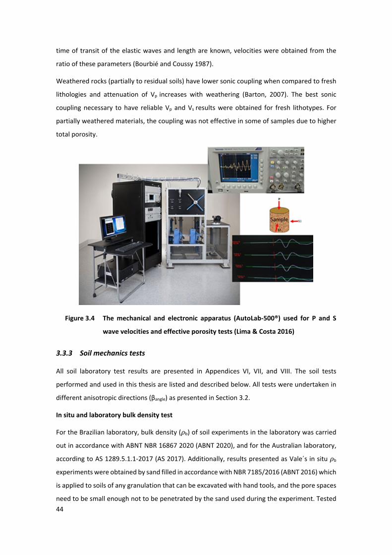
44
time of transit of the elastic waves and length are known, velocities were obtained from the
ratio of these parameters (Bourbié and Coussy 1987).
Weathered rocks (partially to residual soils) have lower sonic coupling when compared to fresh
lithologies and attenuation of Vp increases with weathering (Barton, 2007). The best sonic
coupling necessary to have reliable Vp and Vs results were obtained for fresh lithotypes. For
partially weathered materials, the coupling was not effective in some of samples due to higher
total porosity.
11 Figure 3.4 The mechanical and electronic apparatus (AutoLab-500®) used for P and S
wave velocities and effective porosity tests (Lima & Costa 2016)
3.3.3 Soil mechanics tests
All soil laboratory test results are presented in Appendices VI, VII, and VIII. The soil tests
performed and used in this thesis are listed and described below. All tests were undertaken in
different anisotropic directions (βangle) as presented in Section 3.2.
In situ and laboratory bulk density test
For the Brazilian laboratory, bulk density (𝜌𝜌b) of soil experiments in the laboratory was carried
out in accordance with ABNT NBR 16867 2020 (ABNT 2020), and for the Australian laboratory,
according to AS 1289.5.1.1-2017 (AS 2017). Additionally, results presented as Vale´s in situ 𝜌𝜌b
experiments were obtained by sand filled in accordance with NBR 7185/2016 (ABNT 2016) which
is applied to soils of any granulation that can be excavated with hand tools, and the pore spaces
need to be small enough not to be penetrated by the sand used during the experiment. Tested
45
material needs to be sufficiently cohesive and strong to avoid deformation during the
experiment.
Natural moisture content test
Natural moisture content of samples was based on removing moisture from samples by
oven-drying until its weight remains constant. Moisture content (%) was calculated from the
sample weight before and after drying. Experiments performed in Australia followed Standards
Association of Australia AS 1289.2.1.1 - 2005 (AS 2005) and NBR 6508/84 (ABNT 1984) for the
Brazilian laboratories.
In situ soil permeability test
In situ soil permeability tests were carried out to determine permeability coefficients of residual
soils and completely weathered rocks. Such experiments were carried on according to ABGE n°
04/1996 (ABGE 1996).
Constant and falling head permeability test
Constant head permeability test (Ks) was used for permeable soils with ks > 10-4 cm/s and the
falling head test for less permeable soils (k < 10-4 cm/s). Tests were performed according to
AS 1289.6.7.1 2001 (AS 2001) for constant head and AS 1289 6.7.2. 2001 (AS 2001a) for falling
head for the Australian laboratories and NBR 14545- 2000 (ABNT 2000) for falling head and NBR
13292 – 1995 (ABNT 1995) for constant head for the Brazilian laboratories.
Particle size distribution and hydrometer tests
Particle size distribution (PSD) is widely used for the estimation of soil hydraulic properties such
as water retention curve (Arya & Paris 1981). Particle size analysis involves the measurement of
mass fractions of gravel, sand, silt and clay and results are basic information for soil classification
systems such as the Unified Soil Classification System (USCS) ASTM D-2847-00 (ASTM 2000).
The hydrometer method is another common procedure for measuring mass fractions of a very
fine soil sample. The weight percentages of sand, silt, and clay are calculated from the density
of an aqueous soil suspension measured by a hydrometer. As suggested by Ashworth et al.
(2001), there are many versions of the procedure, differing in the type of dispersing solution,
the volume of the suspension, the time of settling before taking hydrometer readings, or in the
method of correcting the raw readings.
46
PSD analysis was performed according to AS 1289.3.6.1 -2009 (AS 2009) and the hydrometer
method follows AS 1289.3.6.3.-2003 (AS 2003) for Australian laboratories. For tests performed
at the Brazilian laboratory NBR 7217/1987 (ABNT 1987) was followed.
Atterberg limits tests
The Atterberg limit tests are defined as the water contents corresponding to changes in the
behaviour of fine grain soils (silts and clays). The tests are conducted on remoulded material and
are basically for classification purposes and assessing potential engineering behaviour (Martin
& Stacey 2018).
The limits of consistency, namely plastic limit, and liquid limit are well known as soil Atterberg
limits. Plastic limit is the boundary between semi-solid and plastic state, and liquid limit
separates plastic state from liquid state (Campbell 2001).
Information obtained by Atterberg limits was initially developed to describe transported soils.
However, for residual soils and weathered materials such as weathered itabirites, a method
using Fourier analysis to address the influence of mixing materials in Atterberg limits was
summarised by Martin and Stacey 2018.
Tests were performed according to ASTM 4318 – 2010 (ASTM 2010) for the Australian laboratory
and NBR 7180/84 (ABNT 1984) for the Brazilian laboratory.
Single stage consolidated undrained triaxial compressing test
The triaxial test is considered the standard test for shear strength of soils and it is the most
common and versatile shear strength test. The soil sample is placed in a confining chamber and
axial stress is applied until the failure of the sample.
For rock-like soils types, single stage, isotropic consolidated undrained tests (CIU) were
undertaken to determine the undrained strength (undrained condition) for a known initial
effective stress and a sample assumed fully saturated while monitoring the pore pressure during
shear. This does not allow drainage at all phases of the test, and is the most common test used
for weak, porous, and granular (permeable) materials. Results are presented as total or effective
stress and associated porewater pressure are determined.
Australian and Brazilian laboratory triaxial tests were undertaken according to ASTM
D4767-957181 - 11 (ASTM 1995).
47
Single stage unsaturated direct shear test
The direct shear test was developed in order to describe shear strength of a soil, rock or from
discontinuities of an intact rock or soil (Bardet 1997).
The undrained condition direct shear test (UDS) is conducted when porewater is unable to drain
out of the soil, and the rate of loading is much quicker than the rate at which the porewater is
able to drain out of the soil. As a result, most of the external loading is taken by the porewater,
resulting in an increase in porewater pressure. The tendency of soil to change volume is
suppressed during undrained loading.
Undrained shear strength analyses are presented in this thesis applying the Fredlund et al.
(1978) shear strength equation. Effective shear strength parameters of the soil, along with the
initial matric suction and results from unconfined and confined compression tests are required
for the analysis. The procedure focuses on the use of conventional soil testing techniques to
provide a measure of the angle φb.
Changes in matric suction due to an applied total isotropic pressure can be computed from a
knowledge of the initial conditions of the soil, using a marching forward technique. This
procedure is detailed in Fredlund & Rahardjo (1993). This technique is not required if the matric
suction condition is measured.
During undrained axial compression, the matric suction can increase, decrease, or remain
constant depending upon the pore pressure parameter of the soil.
Tests were performed at the Australian and Brazilian laboratory according to AS 1289.6.2.2
– 1998 (AS 1988) using modified apparatus as presented in Figure 3.5.
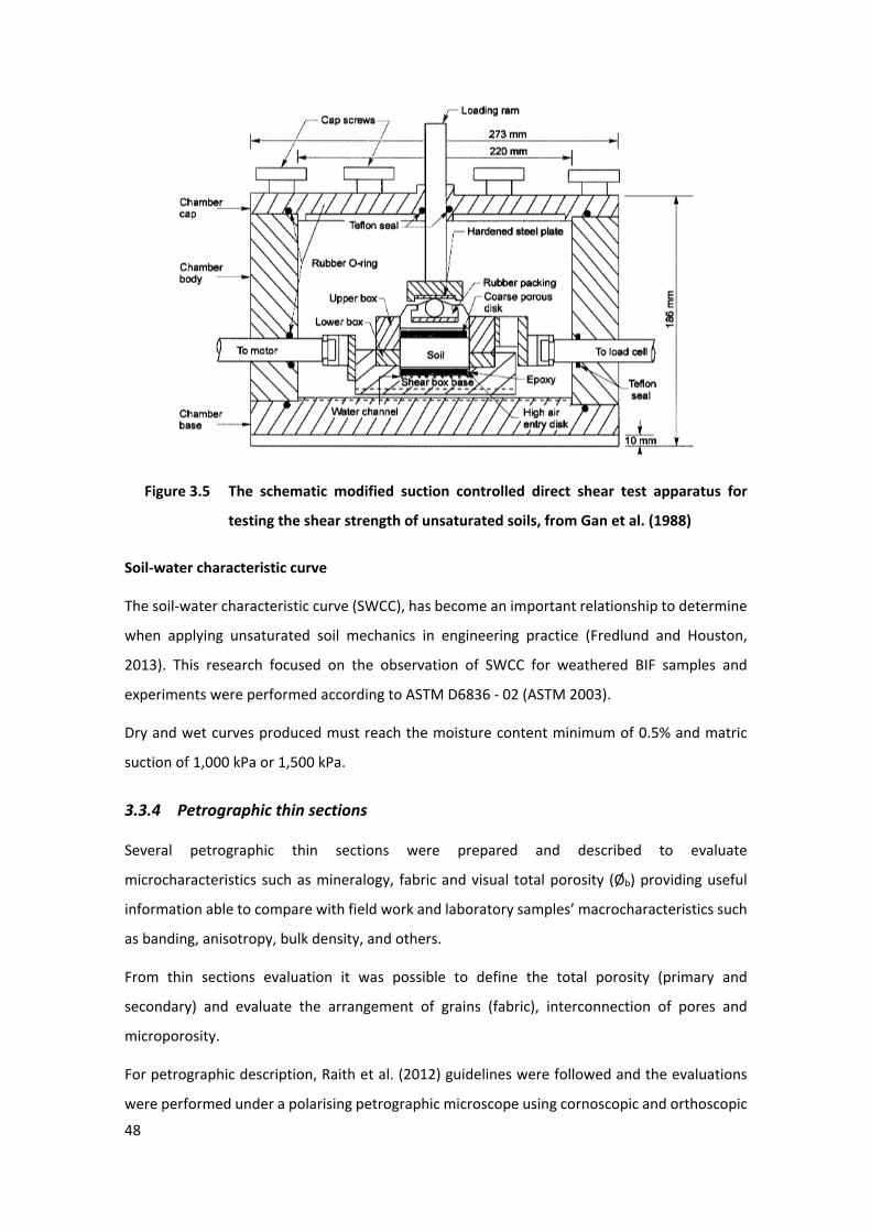
48
12 Figure 3.5 The schematic modified suction controlled direct shear test apparatus for
testing the shear strength of unsaturated soils, from Gan et al. (1988)
Soil-water characteristic curve
The soil-water characteristic curve (SWCC), has become an important relationship to determine
when applying unsaturated soil mechanics in engineering practice (Fredlund and Houston,
2013). This research focused on the observation of SWCC for weathered BIF samples and
experiments were performed according to ASTM D6836 - 02 (ASTM 2003).
Dry and wet curves produced must reach the moisture content minimum of 0.5% and matric
suction of 1,000 kPa or 1,500 kPa.
3.3.4 Petrographic thin sections
Several petrographic thin sections were prepared and described to evaluate
microcharacteristics such as mineralogy, fabric and visual total porosity (Øb) providing useful
information able to compare with field work and laboratory samples’ macrocharacteristics such
as banding, anisotropy, bulk density, and others.
From thin sections evaluation it was possible to define the total porosity (primary and
secondary) and evaluate the arrangement of grains (fabric), interconnection of pores and
microporosity.
For petrographic description, Raith et al. (2012) guidelines were followed and the evaluations
were performed under a polarising petrographic microscope using cornoscopic and orthoscopic
49
illumination modes to evaluate opaque minerals (e.g. iron minerals) and translucid minerals
(e.g. quartz).
Petrographic thin sections descriptions were performed according to anisotropy direction
(perpendicular and parallel to banding) for a better evaluation of the grain and pore size, shape,
texture, distribution, and percentage for fresh and partially weathered BIFs. For completely
weathered lithotypes (WHE, WAI, WQI and WGI) results from Costa (2006) and Vale internal
reports from Zaparolli (2004) were used.
A total of 33 thin sections were prepared at The University of Western Australia’s School of Earth
Science and results were presented by Horta & Costa (2016). Another 13 thin sections from
Costa (2006) were revaluated and considered for this research.
3.4 SOFTWARE USED
Rocdata 5.0 (Rocscience 2021) was the database and processing software used to provide
analysis for strength parameters obtained through laboratorial experiments. This software is
based on Hoek & Brown (1998), Hoek (1990 and 1994) and Hoek et al. (2002) which perform
calculations generating the failure envelopes and strength parameters. Failure envelopes were
plotted in both shear-normal and principal stress space.
Slide 5.0 (Rocscience 2014) was the software used from limit equilibrium analyses and
determination of the safety factor on slope stability analyses performed in the case study
presented in Appendix II.
The experimental data for unsaturated parameters were obtained from the SoilFlux SoilVision
software (SoilVision System LTD. 2009).

50
51
CHAPTER 4. INTACT ROCK STRENGTH CHARACTERISTICS AND ELASTIC
STATIC PROPERTIES OF FRESH BRAZILIAN BANDED IRON FORMATIONS
This chapter presents the first unpublished manuscript.
ABSTRACT
In recent decades, a worldwide iron ore boom has fuelled a rapid increase in pit depths of
Brazilian iron ore mines, especially at mines located in the Iron Quadrangle. This has been due to
environmental restrictions and urban pressure on the lateral expansion of mines. For this reason,
the friable material has been mined and the presence of fresh banded iron formations on final
slopes has become more plentiful, and failure mechanisms and slope instability controlled by
discontinuities and hard rock behaviour have become more common. To support this new
challenge, in mines where instabilities were mainly composed of hard rock materials, rock
mechanics approaches became necessary. These approaches must be based on reliable
geological, structural, and geotechnical investigations supported by laboratory test databases.
In this context, an extensive geological and geotechnical field investigation and laboratory
testing have been conducted to determine the intact rock strength, elastic parameters and
geomechanical behaviour of brittle, hard and fresh banded iron formations (BIF), locally defined
and divided into four main types: fresh quartzitic, amphibolitic and dolomitic itabirites and hard
hematitite.
Laboratory tests undertaken to support the studies include uniaxial compressive strength (UCS),
P wave velocity and bulk density used to define strength and deformability parameters and
establish correlations with Young’s modulus and Poisson’s ratio. The interrelationships were
based on regression curves and the respective coefficients of determination was established to
support research statements. An extra challenge to determine these parameters and correlations
is created by the anisotropy observed for these rock type.
Geological and geomechanical field evaluations, and petrographic thin sections were used to
establish correlations between microtexture, mineralogical composition and macro
characteristics observed on mine slopes. The study focused on the itabirites which exhibit typical
compositional metamorphic banding (heterogeneity), hematitite with no clear heterogeneity
identified, and other geological features to define anisotropy ratio and other characteristics in
BIF.
52
Empirical correlations and adjusted regression curve equations between rock strength, elastic
parameters, and physical properties for different types of fresh BIF were identified. Such
equations can be used to estimate geotechnical parameters, establishing, and identifying
patterns of geomechanical behaviour of the BIF deposits.
Using such approaches, hard hematitite, quartzitic, and amphibolitic itabirites exhibited the
higher intact rock strengths with similar mean values, followed by the dolomitic itabirite with
lower-strength values. P wave velocity is higher for hard hematitite and relatively lower for
itabirites, in some instances following the bulk density reduction. However, it is influenced by the
heterogeneity defined by the main non-iron mineral.
For all BIF types, minor changes in bulk density induced by the heterogeneity, the mineralogical
composition and rock fabric are responsible for variations in the rock mass strengths and elastic
parameters. Anisotropic effects induced by typical banding are not significant for hard
hematitites (isotropic material) and represent a low influence for fresh quartzitic and
amphibolitic itabirites (low anisotropy degree), and a slightly higher anisotropic effect is
observed for fresh dolomitic itabirites (FDI) (low to medium anisotropy degree).
Additionally, qualitative evaluations of the scale effect related to the thickness of the
compositional metamorphic banding (heterogeneity) proved to be an important characteristic
that controls the intact rock strength and other parameters as P wave velocity, and bulk density.
Relative empirical correlations were obtained mainly for fresh quartzitic and amphibolitic
itabirites, between UCS, P wave velocity, bulk density, and elastic parameters providing a reliable
tool to intercorrelate different parameters, assist where there is a lack of laboratory test
information, and establishing the intact rock and elastic behaviour of fresh BIF.
4.1 INTRODUCTION
In recent decades, a booming world iron ore market has pressed local and global iron ore mines
to increase their production by developing innovative technologies, opening new mines, and
expanding existing mines, not only in width but mainly in depth, to meet this high demand.
In this period, iron ore mines located in the Iron Quadrangle, Brazil were especially affected by
environmental and social pressures to reduce expansion of the mining footprint. The expansion
was based on technological development and increase of depth in existing mines. With pit
depths going beyond 500 m, the former pit designs, based on soil like behaviour for friable
material, are no longer valid.
53
These iron ore mines are developed in banded iron formations (BIF) deposits, originally
described by Dorr (1969) as a high-grade ore, called hematite (most recently denominated as
hematitite) and a low-grade ore, called itabirite. The original mineralogical composition of non-
iron bands, consisting of dolomitic, amphibolitic and quartzitic layers are used to differentiate
itabirite types. In addition, those lithotypes are the hardest (fresh) BIF seen in Iron Quadrangle
iron ore mines.
For the deeper mines, the pit slopes are characterised by a full range of residual soil fresh rocks,
such that both soil and rock mechanics principles must be applied to represent these material
behaviours. Over the next decades, it is expected that the mines increase in depth, up to 700 m.
In this future scenario, hard rocks will be responsible for more than 70% of the final slope. In the
forthcoming mines, the complete understanding of intact rock, and rock mass strength,
discontinuity characteristics and strength, and in situ stress will form the basis required for any
pit slope design. Currently, there is a lack of geomechanical information of these materials, and
this is the main reason for studying these lithotypes.
Previous studies show, for these hard rocks, even belonging to the same rock type, a large
scattering in strength and elastic parameters. It is crucial to ensure a proper evaluation of intact
rock strength and elastic parameters, as well as geological and geotechnical characteristics to
understand the behaviour of different types and the influence of anisotropy and heterogeneity
on slope stability analyses and design. In this study, the focus was on intact rock characterisation
and thus an investigation of the discontinuities was not considered, even though it has been
recognised by the authors as an important aspect of the analyses of slope stability and failure
mechanisms.
Based on geological and geotechnical field investigation, thin sections evaluation, P wave
velocity propagation, unconfined compressive strength (UCS) and bulk density (𝜌𝜌b) tests, this
study proposes empirical correlations curves and equations between rock strength, static elastic
parameters (Young´s modulus and Poisson’s ratio) and petrophysical parameters for fresh BIF.
4.2 OBJECTIVES AND APPROACHES
Many studies have been undertaken to determine and establish relationships among
petrophysical and intact rock strength for several rock types. From these, only a few studies have
been focused on BIF. This research presents petrophysical, intact rock strength and elastic static
properties results for several Brazilian BIF, rock types occurring at the Iron Quadrangle, Brazil,
with the aim of establishing correlations by the regression technique (linear or nonlinear). The
degree of association between these variables was measured by the coefficient of
54
determination in an attempt to derive reliable empirical approaches for a better comprehension
of geomechanical and anisotropic behaviour, and to provide basic statistical correlations.
The aims of this research are to define, for the studied fresh BIF types, intact rock strength and
elastic characteristics, with values based on laboratory tests, geological and geomechanical field
characteristics and intrinsic correlations. The aims are summarised below:
• Evaluate and compare for different types of BIF present the intact rock strength, elastic
parameters, and petrophysical properties.
• Evaluate the influence of the anisotropy and heterogeneity, defined by the
metamorphic banding, for the different types of BIF.
• Establish a correlation between petrophysical properties, geological (macro and micro)
properties and intact rock strength and elastic parameters.
The research approach focuses on intact rock properties, assessing the effect of physical
heterogeneity and anisotropy to establish a practical estimate of properties and correlations
that could replace the lack of rock strength and elastic parameters. These correlations, to be
valuable, must consider mechanical and elastic rock properties as a function of petrophysical
characteristics such as mineralogical composition, thin section total porosity, bulk density, and
fabric of each lithotype.
Based on a considerable number of UCS tests, P wave velocity, bulk density, and correlated
geological/geotechnical (macro and micro) and rock fabric characteristics, it is expected for
these types of rocks to be able to determine strength and elastic parameters and will ultimately
help to optimise pit slope designs and promote a better understanding of potential failure
mechanisms and, in turn, lead to a reduced risk of slope failure by allowing an improvement of
operational productivity and safety of iron ore mines. These results are also useful for crusher
hardness definition, optimised design of blasting operations, digging equipment capability, and
other mining operation and planning applications.
To address this work, a PhD research project was undertaken by the lead author at the Australian
Centre for Geomechanics, School of Civil, Environmental and Mining Engineering, The University
of Western Australia, sponsored by Vale S.A. The main aim of the thesis was to investigate the
complete weathering profile characteristics, from fresh and hard to weak residual soil of BIF
from several Brazilian iron ore mine sites.
This chapter summarises the key geological and geotechnical characteristics of four fresh and
hard BIF types based on site investigations and petrographic thin sections description.
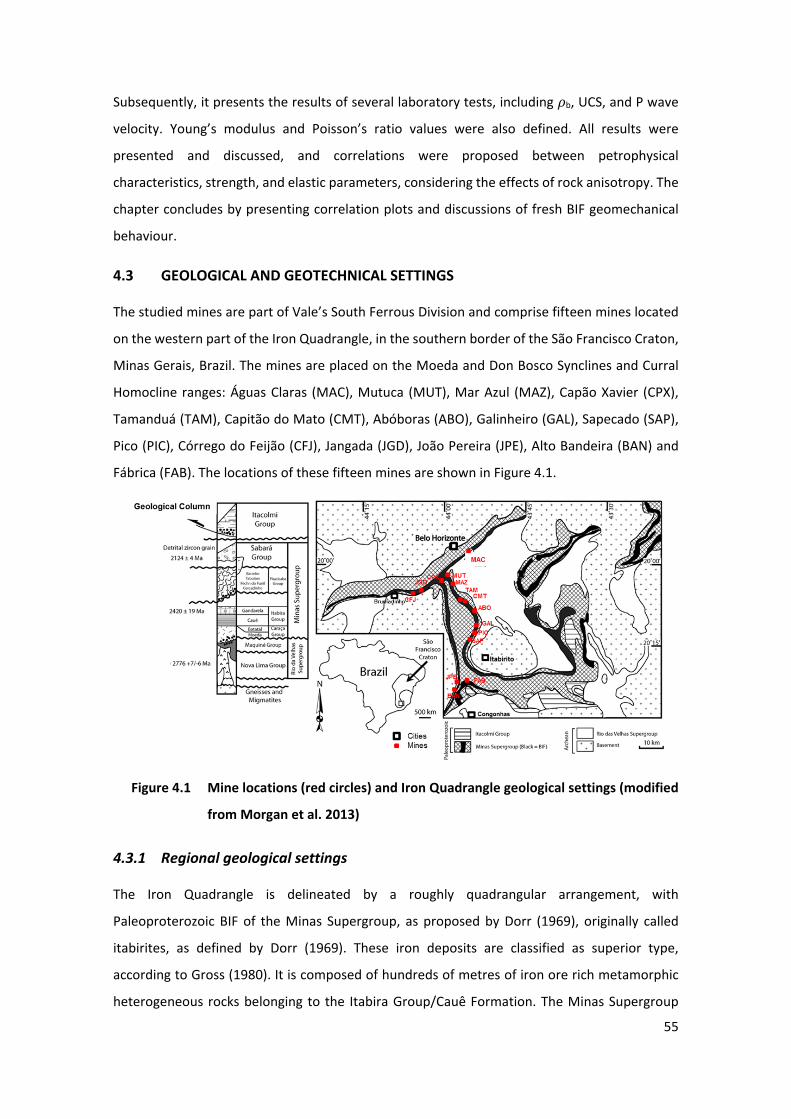
55
Subsequently, it presents the results of several laboratory tests, including 𝜌𝜌b, UCS, and P wave
velocity. Young’s modulus and Poisson’s ratio values were also defined. All results were
presented and discussed, and correlations were proposed between petrophysical
characteristics, strength, and elastic parameters, considering the effects of rock anisotropy. The
chapter concludes by presenting correlation plots and discussions of fresh BIF geomechanical
behaviour.
4.3 GEOLOGICAL AND GEOTECHNICAL SETTINGS
The studied mines are part of Vale’s South Ferrous Division and comprise fifteen mines located
on the western part of the Iron Quadrangle, in the southern border of the São Francisco Craton,
Minas Gerais, Brazil. The mines are placed on the Moeda and Don Bosco Synclines and Curral
Homocline ranges: Águas Claras (MAC), Mutuca (MUT), Mar Azul (MAZ), Capão Xavier (CPX),
Tamanduá (TAM), Capitão do Mato (CMT), Abóboras (ABO), Galinheiro (GAL), Sapecado (SAP),
Pico (PIC), Córrego do Feijão (CFJ), Jangada (JGD), João Pereira (JPE), Alto Bandeira (BAN) and
Fábrica (FAB). The locations of these fifteen mines are shown in Figure 4.1.
13 Figure 4.1 Mine locations (red circles) and Iron Quadrangle geological settings (modified
from Morgan et al. 2013)
4.3.1 Regional geological settings
The Iron Quadrangle is delineated by a roughly quadrangular arrangement, with
Paleoproterozoic BIF of the Minas Supergroup, as proposed by Dorr (1969), originally called
itabirites, as defined by Dorr (1969). These iron deposits are classified as superior type,
according to Gross (1980). It is composed of hundreds of metres of iron ore rich metamorphic
heterogeneous rocks belonging to the Itabira Group/Cauê Formation. The Minas Supergroup
56
comprises, from bottom to top, Caraça, Itabira, Piracicaba and Sabará groups and a sequence of
psammitic pelitic rocks, all being superimposed by the Itacolomi Group (Dorr 1969).
Below that sequence is the Archean greenstone terrains of the Rio das Velhas Supergroup and
domes of Archean and Proterozoic crystalline rocks (Machado & Carneiro 1992; Machado et al.
1989; Noce 1995).
According to Chemale Jr et al. (1994), the regional structure is the result of two main
deformational superimposed events. The first produced the nucleation of regional synclines in
the uplift of the gneissic domes during the Transamazonian Orogenesis (2.1–2 Gyr), and the
second is related to an east–west verging thrust fault belt of Pan African/Brazilian age
(0.8–0.6 Gyr) described by Marshak & Alkmim (1989). This last event deformed the earlier
structures and was responsible for the east–west deformational gradient.
Hertz (1978) described an eastward increase in the metamorphic grade and followed the
deformational gradient from greenschist to lower amphibolite’s facies.
The Cauê Formation (Itabira Group) hosting the BIF is a 350 m thick marine chemical sequence,
dated 2.4 ± 0.19 Gyr (Babinski et al. 1995).
The Iron Quadrangle BIF are Paleoproterozoic, metamorphic and heterogeneous banded rocks,
presenting a millimetre to centimetre rhythmic alternation banding of iron minerals (hematite,
martite and magnetite), and non-iron minerals (quartz, dolomite, and amphibolite). Dorr (1969)
defined, for this type of iron deposit, two main lithologies: hematite, recently redescribed by
Selmi et al. (2009) as hematitite, the high-grade ore (Fe ≥ 62%); and the low-grade ore, the
itabirite (30% < Fe < 62%), with three compositional types or lithotypes, according to the
presence and relative abundance of gangue minerals: quartzitic, dolomitic and amphibolitic (all
defined as proto-ore). Tectonic, metamorphic, and weathering processes have changed it in
different ways, resulting in multiple sets of iron ore lithotypes.
The studied mines are in the western low metamorphic grade (greenschist) and low strain
domain, nucleated in the Transamazonian event. The main trend of the synclines is north–south,
but the structure has also been deformed around the Bação dome. In the south, it is
interconnected with the Dom Bosco Syncline and is partially truncated by the Engenho Fault
(FAB, JPE and BAN). To the north, the Moeda Syncline is continuous with the Serra do Curral
(Rosière et al. 1993) (Figure 4.1).
The Moeda Syncline (MUT, MAZ, CPX, TAM, CMT, ABO, GAL, PIC, and SAP mines) has been
partially affected by the younger Brazilian tectonic cycle and mainly in the eastern limb with the
57
local development of ductile–brittle to brittle shear zones that cut all lithologies or are
subparallel to the bedding planes. Several strike–slip faults cut across the structure dividing it
into several segments.
The Serra do Curral (MAC, JGD and CFJ) represents the overturned southeastern limb of a
truncated northwest verging syncline–anticline couple highly strained and rotated by the right
lateral movement of the northeast–southwest trending oblique ramp of thrust fault as
supported by Chemale Jr et al. (1994). In this segment, the northwestward inverted limb of a
syncline is truncated near to the contact of the Minas Supergroup in the underlying Rio das
Velhas Supergroup by shear zones related to the thrust.
4.3.2 BIF geological and geotechnical settings
Compositional metamorphic banding is the most typical itabirite characteristic and is considered
to define a heterogeneity. This variation could have been controlled and disturbed by the
original sedimentary bedding, tectonic setting, metamorphic grade, hypogene or supergene
processes and weathering, as the superposition of these processes causes partial or total
mineralogical and textural changes. Studies of BIF conducted by Rosière et al. (2001) for the
western side of the Iron Quadrangle indicate a very low internal deformation by plastic flow of
the minerals with the ductile deformation accommodated mostly by buckling and flexural gliding
with local development of a spaced cleavage. A continuous schistosity and an anastomosing
foliation occur, related to discontinuously developed shear zones. Brecciated zones are usually
related to sites of local water pressure build-up, during the percolation of hydrothermal fluids.
Not considering the controversy about the supergene (groundwater leaching) or hypogene
(hydrothermal water leaching) genesis for these large, rich, and weak Iron Quadrangle ore
deposits, this study is focused on the three main hard and fresh itabirites proto-ore, and hard
hematitite, produced either tectonically or by a hydrothermal event. This variation is
conditioned by the original composition of sediments, the intensity of deformation, and the
degree of metamorphism and hydrothermal alteration imposed. Tectonic structures produced
a large variety of textural features due to the development of discontinuity planes, and
microstructures resulting from different tectonic types of itabirite.
Hematitite and itabirites are locally subdivided by using rock strength characteristics (hardness),
rated in technological crusher laboratory tests, used to simulate the industrial process for better
control of mining operations, which are also used for geotechnical purposes as a rock strength
index. This test consists of crushing a sample to less than 31.5 mm and passing it through the
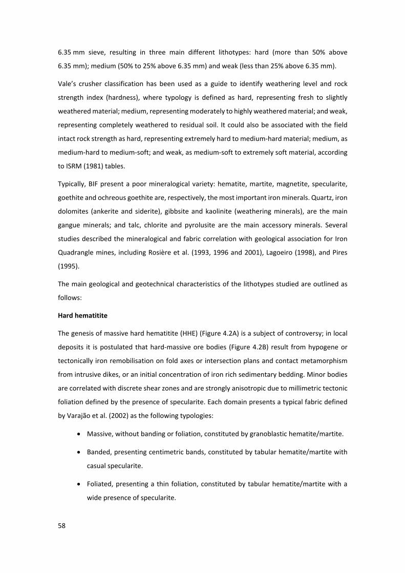
58
6.35 mm sieve, resulting in three main different lithotypes: hard (more than 50% above
6.35 mm); medium (50% to 25% above 6.35 mm) and weak (less than 25% above 6.35 mm).
Vale’s crusher classification has been used as a guide to identify weathering level and rock
strength index (hardness), where typology is defined as hard, representing fresh to slightly
weathered material; medium, representing moderately to highly weathered material; and weak,
representing completely weathered to residual soil. It could also be associated with the field
intact rock strength as hard, representing extremely hard to medium-hard material; medium, as
medium-hard to medium-soft; and weak, as medium-soft to extremely soft material, according
to ISRM (1981) tables.
Typically, BIF present a poor mineralogical variety: hematite, martite, magnetite, specularite,
goethite and ochreous goethite are, respectively, the most important iron minerals. Quartz, iron
dolomites (ankerite and siderite), gibbsite and kaolinite (weathering minerals), are the main
gangue minerals; and talc, chlorite and pyrolusite are the main accessory minerals. Several
studies described the mineralogical and fabric correlation with geological association for Iron
Quadrangle mines, including Rosière et al. (1993, 1996 and 2001), Lagoeiro (1998), and Pires
(1995).
The main geological and geotechnical characteristics of the lithotypes studied are outlined as
follows:
Hard hematitite
The genesis of massive hard hematitite (HHE) (Figure 4.2A) is a subject of controversy; in local
deposits it is postulated that hard-massive ore bodies (Figure 4.2B) result from hypogene or
tectonically iron remobilisation on fold axes or intersection plans and contact metamorphism
from intrusive dikes, or an initial concentration of iron rich sedimentary bedding. Minor bodies
are correlated with discrete shear zones and are strongly anisotropic due to millimetric tectonic
foliation defined by the presence of specularite. Each domain presents a typical fabric defined
by Varajão et al. (2002) as the following typologies:
• Massive, without banding or foliation, constituted by granoblastic hematite/martite.
• Banded, presenting centimetric bands, constituted by tabular hematite/martite with
casual specularite.
• Foliated, presenting a thin foliation, constituted by tabular hematite/martite with a
wide presence of specularite.
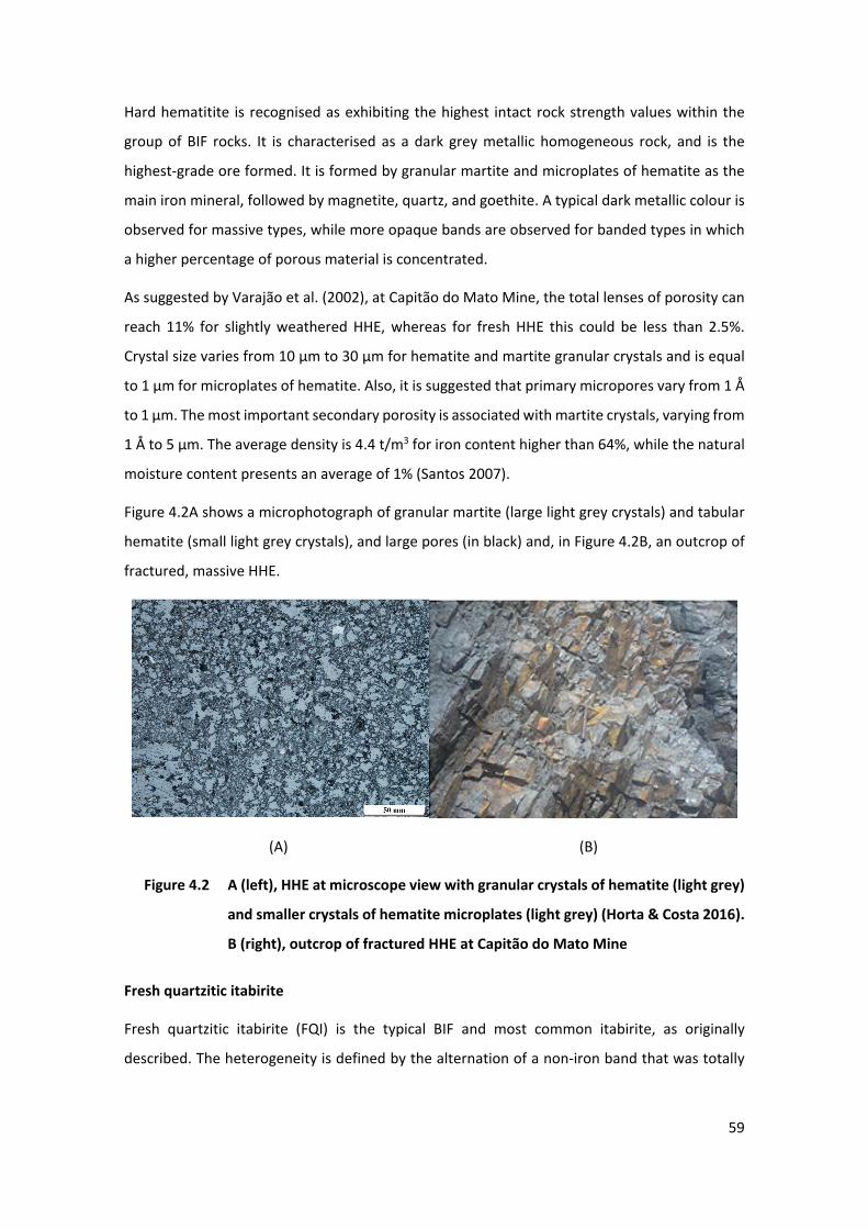
59
Hard hematitite is recognised as exhibiting the highest intact rock strength values within the
group of BIF rocks. It is characterised as a dark grey metallic homogeneous rock, and is the
highest-grade ore formed. It is formed by granular martite and microplates of hematite as the
main iron mineral, followed by magnetite, quartz, and goethite. A typical dark metallic colour is
observed for massive types, while more opaque bands are observed for banded types in which
a higher percentage of porous material is concentrated.
As suggested by Varajão et al. (2002), at Capitão do Mato Mine, the total lenses of porosity can
reach 11% for slightly weathered HHE, whereas for fresh HHE this could be less than 2.5%.
Crystal size varies from 10 μm to 30 μm for hematite and martite granular crystals and is equal
to 1 μm for microplates of hematite. Also, it is suggested that primary micropores vary from 1 Å
to 1 μm. The most important secondary porosity is associated with martite crystals, varying from
1 Å to 5 μm. The average density is 4.4 t/m3 for iron content higher than 64%, while the natural
moisture content presents an average of 1% (Santos 2007).
Figure 4.2A shows a microphotograph of granular martite (large light grey crystals) and tabular
hematite (small light grey crystals), and large pores (in black) and, in Figure 4.2B, an outcrop of
fractured, massive HHE.
(A) (B)
14 Figure 4.2 A (left), HHE at microscope view with granular crystals of hematite (light grey)
and smaller crystals of hematite microplates (light grey) (Horta & Costa 2016).
B (right), outcrop of fractured HHE at Capitão do Mato Mine
Fresh quartzitic itabirite
Fresh quartzitic itabirite (FQI) is the typical BIF and most common itabirite, as originally
described. The heterogeneity is defined by the alternation of a non-iron band that was totally
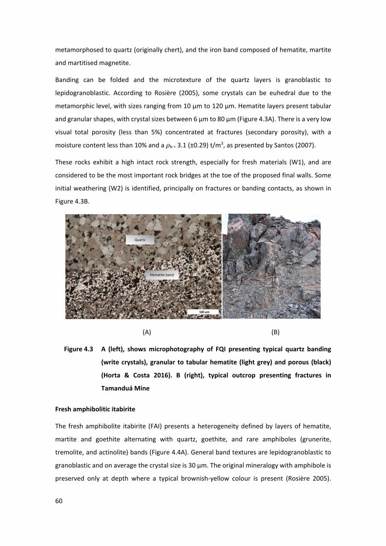
60
metamorphosed to quartz (originally chert), and the iron band composed of hematite, martite
and martitised magnetite.
Banding can be folded and the microtexture of the quartz layers is granoblastic to
lepidogranoblastic. According to Rosière (2005), some crystals can be euhedral due to the
metamorphic level, with sizes ranging from 10 µm to 120 µm. Hematite layers present tabular
and granular shapes, with crystal sizes between 6 µm to 80 µm (Figure 4.3A). There is a very low
visual total porosity (less than 5%) concentrated at fractures (secondary porosity), with a
moisture content less than 10% and a 𝜌𝜌b = 3.1 (±0.29) t/m3, as presented by Santos (2007).
These rocks exhibit a high intact rock strength, especially for fresh materials (W1), and are
considered to be the most important rock bridges at the toe of the proposed final walls. Some
initial weathering (W2) is identified, principally on fractures or banding contacts, as shown in
Figure 4.3B.
(A) (B)
15 Figure 4.3 A (left), shows microphotography of FQI presenting typical quartz banding
(write crystals), granular to tabular hematite (light grey) and porous (black)
(Horta & Costa 2016). B (right), typical outcrop presenting fractures in
Tamanduá Mine
Fresh amphibolitic itabirite
The fresh amphibolite itabirite (FAI) presents a heterogeneity defined by layers of hematite,
martite and goethite alternating with quartz, goethite, and rare amphiboles (grunerite,
tremolite, and actinolite) bands (Figure 4.4A). General band textures are lepidogranoblastic to
granoblastic and on average the crystal size is 30 µm. The original mineralogy with amphibole is
preserved only at depth where a typical brownish-yellow colour is present (Rosière 2005).
Quartz
Hematite band
500 μm
61
It exhibits a very low effective porosity (less than 5%), while moisture content is 10% and 𝜌𝜌b =
2.8 (±0.46) t/m3, as presented by Santos (2007).
Due to weathering, the amphibolic minerals easily change to fibrous goethite and, due to the
deep weathering profile, it is usually difficult to obtain ‘fresh FAI’ (with amphibole) at the surface
or shallow depths that has not been influenced by some mineral degradation. For this reason,
in this chapter, the so-called ’fresh FAI’ will also consider the slightly weathered FAI (W2), even
in the absence of amphibolitic minerals and rare W1 samples.
The intact rock strength of the FAI is equivalent to other itabirites and is still strong when
classified as W2 where some weathering and discoloration (dark yellow or brown) can be
observed in fractures and banding layers (Figure 4.4B).
(A) (B)
16 Figure 4.4 A (left), shows microphotography of a FAI highlighting the presence of fibrous
goethite an amphibolite acicular old crystal (dark fibre minerals) immerse on
quartz bands (Horta & Costa 2016). B (right), shows a typical slope of folded
and fractured FAI at Jangada Mine
Fresh dolomitic itabirite
As presented by Rosière (2005), the heterogeneity is defined by the millimetric to centimetric
pink or white iron dolomite and lower percentages of iron carbonates and quartz bands. These
layers occur interbedded with dark grey iron bands comprised of tabular hematite, martite, and
martitised magnetite bands. The most important accessory minerals are sericite, talc, and
chlorite. The non-iron minerals vary in size from 2 µm to 15 µm, and the iron bands present
crystal size varying from 5 µm to 20 µm (Figure 4.5A).
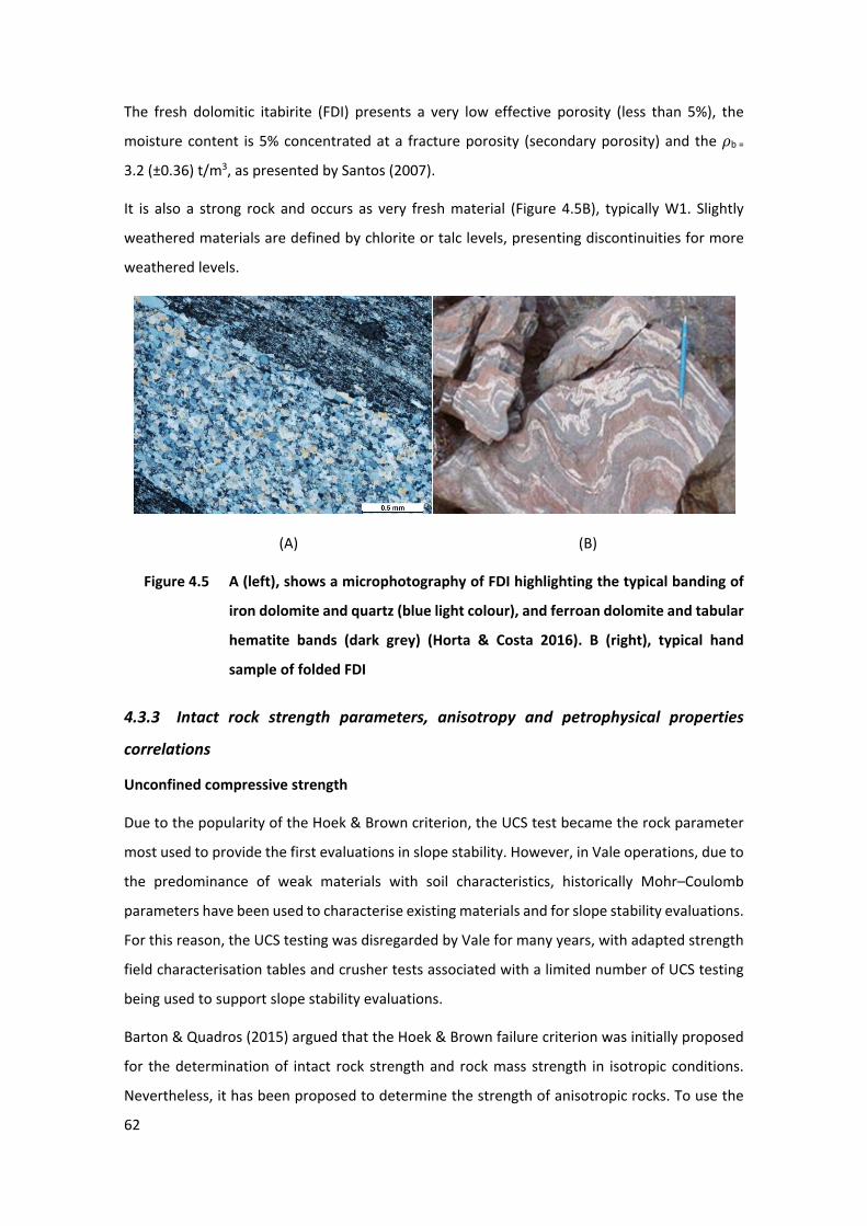
62
The fresh dolomitic itabirite (FDI) presents a very low effective porosity (less than 5%), the
moisture content is 5% concentrated at a fracture porosity (secondary porosity) and the 𝜌𝜌b =
3.2 (±0.36) t/m3, as presented by Santos (2007).
It is also a strong rock and occurs as very fresh material (Figure 4.5B), typically W1. Slightly
weathered materials are defined by chlorite or talc levels, presenting discontinuities for more
weathered levels.
(A) (B)
17 Figure 4.5 A (left), shows a microphotography of FDI highlighting the typical banding of
iron dolomite and quartz (blue light colour), and ferroan dolomite and tabular
hematite bands (dark grey) (Horta & Costa 2016). B (right), typical hand
sample of folded FDI
4.3.3 Intact rock strength parameters, anisotropy and petrophysical properties
correlations
Unconfined compressive strength
Due to the popularity of the Hoek & Brown criterion, the UCS test became the rock parameter
most used to provide the first evaluations in slope stability. However, in Vale operations, due to
the predominance of weak materials with soil characteristics, historically Mohr–Coulomb
parameters have been used to characterise existing materials and for slope stability evaluations.
For this reason, the UCS testing was disregarded by Vale for many years, with adapted strength
field characterisation tables and crusher tests associated with a limited number of UCS testing
being used to support slope stability evaluations.
Barton & Quadros (2015) argued that the Hoek & Brown failure criterion was initially proposed
for the determination of intact rock strength and rock mass strength in isotropic conditions.
Nevertheless, it has been proposed to determine the strength of anisotropic rocks. To use the
63
criterion in this way, careful parameter selection is necessary, especially for the UCS (σci) and the
material constants (mi) and (s). Moreover, determining the minimum and maximum intact rock
strengths due to rock anisotropy is very important when selecting the characteristic values of
the intact rock.
It is recognised that slope stability in hard and fresh rocks is controlled mostly by kinematic
freedom and the shear strength of discontinuities. However, intact rock strength parameters
are fundamental to characterise and evaluate slope stability. Thus, UCS is ideally obtained from
laboratory tests, but can also be obtained by correlation index tests (e.g. point load, P wave
velocity propagation or Schmidt tests). In some cases, bulk density or other physical parameters
can be used as a simple measurement to estimate the UCS (Marques et al. 2010).
Petrophysical properties and correlations
It is recognised that other physical characteristics such as porosity, bulk density, mineralogical
composition, crystal size, and fabric are directly responsible for variations in the strength of
intact rock. However, few studies of the interrelationship between intact rock strength and
petrophysical parameters have been established worldwide for BIF.
In this regard, conclusions from Thomson (1963) for Australian iron ores have suggested a
theoretical hematite–quartz curve used to determine the 𝜌𝜌b and appropriate iron content
approximation. Correlations presented by Aylmer et al. (1978) have associated 𝜌𝜌b, iron grade
and porosity for Mount Tom Price iron ore. Studies by Box & Reid (1976) for the iron ore
formation at Cockatoo Island attempted to correlate true specific gravity with iron content and
the influence of porosity. Finally, studies by Nel (2007), developed for Sishen iron deposits in
South Africa, developed a direct correlation between porosity and dry bulk density, providing a
reliable calculation index.
Static and dynamic elastic properties and correlations
Classical rock mechanics provides various techniques for determining the elastic parameters,
the most widely employed being stress-strain curves obtained from destructive compressive and
tensile rock tests. Most recently, a start has been made on using non-destructive tests based on
acoustic wave velocity propagation to obtain such parameters.
Timoshenko (1983) defines strain as a change in geometry, orientation, volume, and position
induced by either a load or unload of stress in a certain period of time (Dantas 2018). For each
rock type (homogeneous or heterogeneous) and load (constant or variable) applied it is possible
to write the constitutive stress-strain laws resulting in various deformability parameters. Such
64
parameters are derived directly in situ or through laboratory testing, and indirectly from rock
mass classification using correlations. Laboratory tests are categorised as static, when samples
are submitted to loading or unloading that induces different equilibrium stresses, and dynamic
elastic parameters are obtained in response to a cyclic, rapid energy source such as an acoustic
wave emission.
Using specific laboratory testing, Kearey et al. (2009) showed that the elastic modulus can be
obtained indirectly by calculating acoustic emission velocity (mechanical seismic waves) within
a rock specimen resulting from particle vibrations triggered by an energy source. It differs from
the elastic modulus and material density and can be divided into two types: compressive waves
or P waves, which move through the propagation direction, and shearing waves or S waves,
which move perpendicularly to the propagation path.
For isotropic materials, the seismic pulse is perpendicular to the wavefront, and wave
propagation velocity is defined by the rate at which the acoustic pulse travels through the
material.
Kearey et al. (2009) also explain that wave velocity is a function of the mineralogical
composition, texture, porosity, and the presence of fluids. These factors severely affect the
P wave, whereas the S wave did not propagate through discontinuities or empty spaces. Several
characteristics of P and S wave velocity for common lithotypes are listed below:
• Felsic igneous rocks have lower speeds relative to mafic rocks.
• The velocity reduces as the number of discontinuities (fractures) increases.
• Porous sedimentary rocks present velocity dispersion associated with the porosity and
density correlation, with higher velocities for high density and low porosity, and lower
velocities for low density and high porosity. It also depends on the cementation grade,
consolidation, and other factors.
• In contrast to those with smaller crystals, lithotypes with the same mineral
composition with larger crystals present higher velocities.
• Higher wave velocity occurs parallel to the anisotropy direction and lower velocity is
observed in the direction perpendicular to anisotropy in metamorphic rocks. These
changes are associated with mineral and porous alignment, and the set of
discontinuities. Lower velocities are controlled by the weakness planes along banding
and schistosity. Otherwise, higher velocities are associated with the strongest crystal
contacts along the anisotropy direction.
65
• For the same reason, the P wave velocity anisotropy decreases with stress and
increases with temperature. The latter effect may be due to the widening of pores and
microcracks during the expansion of the sample due to thermal stress.
As presented in Deere & Miller (1966), it must be assumed that elastic constants determined
using acoustic wave emission, which defines the elastic behaviour, are dependent on a broad
range of variables such as rock type, mineralogical composition, rock texture and structure, grain
size and shape, density, porosity, degree of anisotropy, porewater, confining pressure, moisture
content, stress amplitude, rate and duration of loading, temperature, weathering and alteration
zones, and joint properties and defining the most important variable could be a difficult task.
The use of acoustic wave propagation velocity to determine intact rock strength have been used
for several typologies by a number of researchers including Inoue & Ohome (1981) for weak
rocks. Gaviglio (1989) focused on rock density, and Kaharaman (2001) and Yasar & Endogan
(2004) applied it to carbonate rocks. Based on its close relation to the intact rock properties,
structure, and texture, these methods have been used by major global mining companies such
as Vale S.A. Later studies and subsequent standard rock strength tests have confirmed the
validity of static and dynamic comparisons using non-destructive sonic wave measures
techniques. Furthermore, the low cost, repeatability, and speed of acoustic emission tests are
attractive characteristics.
According to Oyler et al. (2010), for coal mines, the results of regression analyses of the
relationships between P wave velocity and UCS tests are meaningful and are routinely used to
determine the σci of the coal seam.
Acoustic emission can be coupled with laboratory static tests, facilitating constant monitoring in
different directions during the stress level increase. As stated in White (1983), it is possible to
calculate the dynamic elastic constants such as Young’s modulus (Edyn), Poisson’s ratio (νdyn),
shearing modulus (Gdyn) and incompressibility modulus (Kdyn) based on compressional wave
velocity (VP), shear wave velocity (Vs) and the sample’s bulk density (𝜌𝜌b) by the application of the
elasticity theory. Equations 4.1, 4.2 and 4.3 show the relationship between dynamic elastic
constants, 𝜌𝜌b, and elastic wave velocities modified from White (1983):
Dynamic Poisson’s ratio correlations:
𝑣𝑣𝑑𝑑𝑑𝑑𝑚𝑚 =(𝑉𝑉𝑝𝑝
𝑉𝑉𝑠𝑠� )2−2
2��𝑉𝑉𝑝𝑝
𝑉𝑉𝑠𝑠� �2−1�
(4.1)
66
where:
νdyn = Poisson’s ratio.
VP = compressional wave velocity.
Vs = shear wave velocity.
Dynamic Young’s modulus correlations:
𝐸𝐸𝑑𝑑𝑑𝑑𝑚𝑚 = 𝜌𝜌𝑉𝑉𝑠𝑠2(3𝑉𝑉𝑝𝑝2−4𝑉𝑉𝑠𝑠2)(𝑉𝑉𝑝𝑝2−𝑉𝑉𝑠𝑠2)
(4.2)
where:
Edyn = Young’s modulus.
Compressive wave velocity (Vp) correlations:
Vp2 = 𝐸𝐸𝑑𝑑𝑑𝑑𝑑𝑑(1−υ)ρb(1+υ)(1−2υ)
(4.3)
where:
𝜌𝜌b = bulk density.
ν = Poisson’s ratio.
In this chapter, just one basic mechanism of energy transmission by elastic waves was studied:
compressional waves (P), which propagate through the plug’s axial direction in compression. For
this reason, just Equation 4.3 was applied. A complete evaluation is presented in Chapter 5.
Studies, correlating dynamic elastic proprieties with petrophysical and static strength
parameters on BIF, have been developed by Wassermann et al. (2009) for an oolithic iron mine
in Lorraine, France. The study evaluated damage processes on UCS tests using P wave velocity
and found that mechanical behaviour deduced from strain measurements is dilatant for some
samples and non-dilatant for the others, even when elastic properties indicate damage
processes for all samples. Silva (2014), studying Archean schists from Cuiabá mine, Brazil had
measured permeability, total porosity and elastodynamic properties that show the rigidity of
these rocks and were used to define lithostructural constraints. Regarding iron-oxide
mineralisation in the Blötberget mine, Sweden, Maries et al. (2017) obtained several physical
properties from geophysical logging and laboratory measurements to assess the ore-bearing
rocks by increasing density and dynamic elastic modules measured from the full-waveform
sonic.
67
For BIF in the Iron Quadrangle, the studies by Pereira (2017) using acoustic emission and other
geophysical techniques on well logging, defined rock strength parameters and discontinuity
characteristics to establish RQD and elastic in situ modules. Dantas (2018), using part of this
research database, evaluated, and correlated dynamic and static proprieties in different
anisotropy directions using statistical approaches. The author has shown a well-adjusted
regressive model for fresh itabirites. In general, the levels of the statistical parameters are
improved for initial anisotropy directions with poorly adjusted regression curves after the
elimination of spurious data.
Bulk density is the most direct and easy-to-measure indicator of changes in compactness and
level of alteration of a sample (Van-den Akker & Soane 2005). It is an essential physical property,
which has good correlation with the majority of index properties of rock, mainly with P wave
porosity. Studies by Drake et al. (1963) and Gardner et al. (1974) presented an empirical
correlation equation for Vp and ρb for limestone and granitic rocks.
BIF heterogeneity and anisotropy
An important geological BIF characteristic easily observed and measured on several scales
varying from a few millimetres to several centimetres is the heterogeneity defined by typical
metamorphic banding. This heterogeneity can result in a type of anisotropy described as
transverse isotropy, in which layers have approximately the same rock properties along the
plane of the band and different rock properties across the band. As suggested by Hudson &
Harrison (2000), geomechanically the important rock properties that can be affected by
anisotropy are deformability modulus, strength, brittleness, permeability, and discontinuity
frequency.
Singh et al. (1989) and Ramamurthy (1993) pointed out that metamorphic rocks are mostly
anisotropic due to the effect of schistosity, cleavage and microcracking. For BIF, anisotropy is
defined by its mineralogical composition (metamorphic banding), mineralogical orientation
(alignment of minerals at the same orientation), the porosity induced by the original
composition or weathering, and different bulk densities in each layer. Additionally, secondary
anisotropy directions, defined by schistosity and foliation, are locally found mainly in hematitites
and in itabirites with some discreet shear zones and fold axes.
The compositional metamorphic banding (heterogeneity) is defined by the alternation of iron
and non-iron layers (typical itabiritic metamorphic banding). It is the most important itabirite
feature that dictates the formation of the intact rock strength, and is controlled by iron or non-
iron layer thickness, porosity, and mineral composition. A simple example is observed in zones
68
where the banding contains thicker layers of iron minerals, the itabirite will be denser, with
lower porosity and relative higher strength values.
Ultimately, BIF heterogeneity is responsible for determining the different lithotypes, ranging
from country (waste) rocks such as dolomite, quartzite, and amphibolite (very few or non-iron
bands); they range to high-grade ore (very few or no waste bands) as rich itabirite or hematitite.
This evaluation accords with results presented by Dalstra et al. (2003), that compare the
Hamersley Province iron ore with many global deposits and correlate the proto-ore assemblages
with intermediate iron grades between ore and the host BIF.
For Brazilian BIF, studies by Ribeiro et al. (2014), Santos et al. (2005), and Santos (2007) focused
on evaluating the association between bulk density and iron content for Vale’s iron mines and
concluded that there is a linear positive correlation between the total iron content and the bulk
density. Also, Appendix I presented a first attempt to establish a linear positive correlation
between bulk density, iron content and UCS tests for fresh and hard BIF.
Saroglou & Tsiambaos (2007) found that the engineering behaviour of rock masses is strongly
dependent on the anisotropy present at different scales. In the microscale (intact rock), it
depends on the alignment of the rock crystals (i.e. inherent anisotropy). In the macroscale (rock
masses), with anisotropic structure, it is characterised by distinct bedding or schistosity planes
(structural anisotropy). The inherent strength anisotropy of intact rock, which is the focus of this
chapter, can be determined by the variation of UCS (σci) and characterised by the strength
anisotropy degree (RC), as proposed by Singh et al. (1989), or anisotropic index (IVp) as proposed
by Saragou & Tsiambaros (2007) due to the existence of bedding, foliation and schistosity planes
in both intact rock observed in the macroscale and microscale.
4.4 METHODOLOGY
To evaluate the geological and engineering characteristics of fresh and hard BIF and to achieve
the proposed goals, the research methodology adopted was divided into three phases:
• For the first phase, a field investigation was undertaken, and several samples collected
from outcrops and from core drills for all BIF lithotypes. Geological and geotechnical
information were logged, based on ISRM (1981) suggestions, and physical
characteristics were described (e.g. anisotropy and, banding) to support that analysis
of laboratory test results. Outcrops and samples were photographed for additional
visual information such as anisotropy, banding, type of BIF and discontinuities.
69
• The second phase focused on the description of petrographic thin sections, to evaluate
the rock mineralogy, fabric, total porosity, and to provide information on a microscopic
scale to be compared with field macro characteristics described in the first phase.
• The third phase included the execution and evaluation of all laboratory tests and
results used and complied to determine the intact rock properties together with the
correlations with geological characteristics and geotechnical parameters of each
lithotype obtained during the previous phases. The correlation between anisotropy,
UCS, 𝜌𝜌b, P wave velocity, Poisson’s ratio, and Young’s modulus were established.
Tests results dispersion evaluation
When determining σci, from intact rock strength, it is expected that minor microfractures or
other discontinuities will be present in the tested sample. The difficulty of preparing samples
where there are no visible fractures depends on with the inherent anisotropy of the intact rock,
where the alignment of rock-forming crystals cannot be excluded when determining the intact
rock strength.
Recognised as the most common and widely used strength test for rock mechanics, the UCS test
is also known for its high variances mainly related to sample preparation, imperfections or
geological aspects associated with intrinsic characteristics such as heterogeneities, mineral
veins, anisotropy, microfractures, and other defects or effects. However, high variable results
can also be derived from intrinsic sample characteristics and/or negligence/error during sample
selection and grouping. A sampling validation approach based on grouping by geological
characteristics such as banding type, bulk density, and the presence of typical geological
features, is presented in the Appendices I and II.
The features used to group the samples followed approaches presented in Appendix I as follows:
• Samples were grouped by weathering level W1 and W2 (ISRM 1981a).
• P wave velocity (Vp) measures were used to discard inadequate samples with
inclusions or microfracture.
• As BIF presents a typical 𝜌𝜌b variation, a range was established to separate fresh
itabirites (from 2.7 t/m3 to 3.8 t/m3) from non-iron or waste rock (below 2.7 t/m3) and
hematitite (above 3.8 t/m3), as described by Ribeiro et al. (2014).
• Each sample was photographed before and after testing to identify the main geological
characteristics, failure geometry and modes.
70
• UCS test results were size normalised using the empirical scale effect relationship for
intact strength suggested by Hoek & Brown (1980).
• As the UCS result could present an anisotropy dependency, samples were tested at
several different orientations (βangle) to the plane of anisotropy.
• Geological features such as intense folding, the presence of specularite, matrix
material with a different degree of weathering, and the presence of quartz and calcite
veins and other materials which did not represent the typical itabiritic heterogeneity
were discarded.
• To maintain the same compositional metamorphic banding scale and to avoid the
scaling effects, only samples with centimetre thick layers (i.e. typical banding), were
inspected and evaluated.
Extreme outlier results were removed according to the box plot statistical methodology
(Whitaker et al. 2013). This technique identifies the mild outlier’s values from the quartiles (Qt)
determination, based on Equation 4.4.
Values below the lower inner fence (QtLower):
QtLower = 1Qt - 1.5(3Qt - 1Qt) (4.4)
and values above the upper inner fence (Qtupper) as Equation 4.5:
Qtupper = 3Qt + 1.5(3Qt - 1Qt) (4.5)
where 1Qt is the first quartile and 3Qt is the third quartile.
The 3Qt evaluates database dispersion around a central data leaving 75% of data below the sum
and is defined by Equation 4.5:
3Qt = × + 1.5.IQR (4.5)
The 1Qt evaluates database dispersion around a central data leaving 25% of data below the sum
and is defined by the Equation 4.6.
1Qt = × - 1.5.IQR (4.6)
Interquartile ranges (IQR) measure how spread out from a central data the values are. These
form what are called outliers and are defined by Equation 4.7:
IQR = 3Qt - 1Qt (4.7)
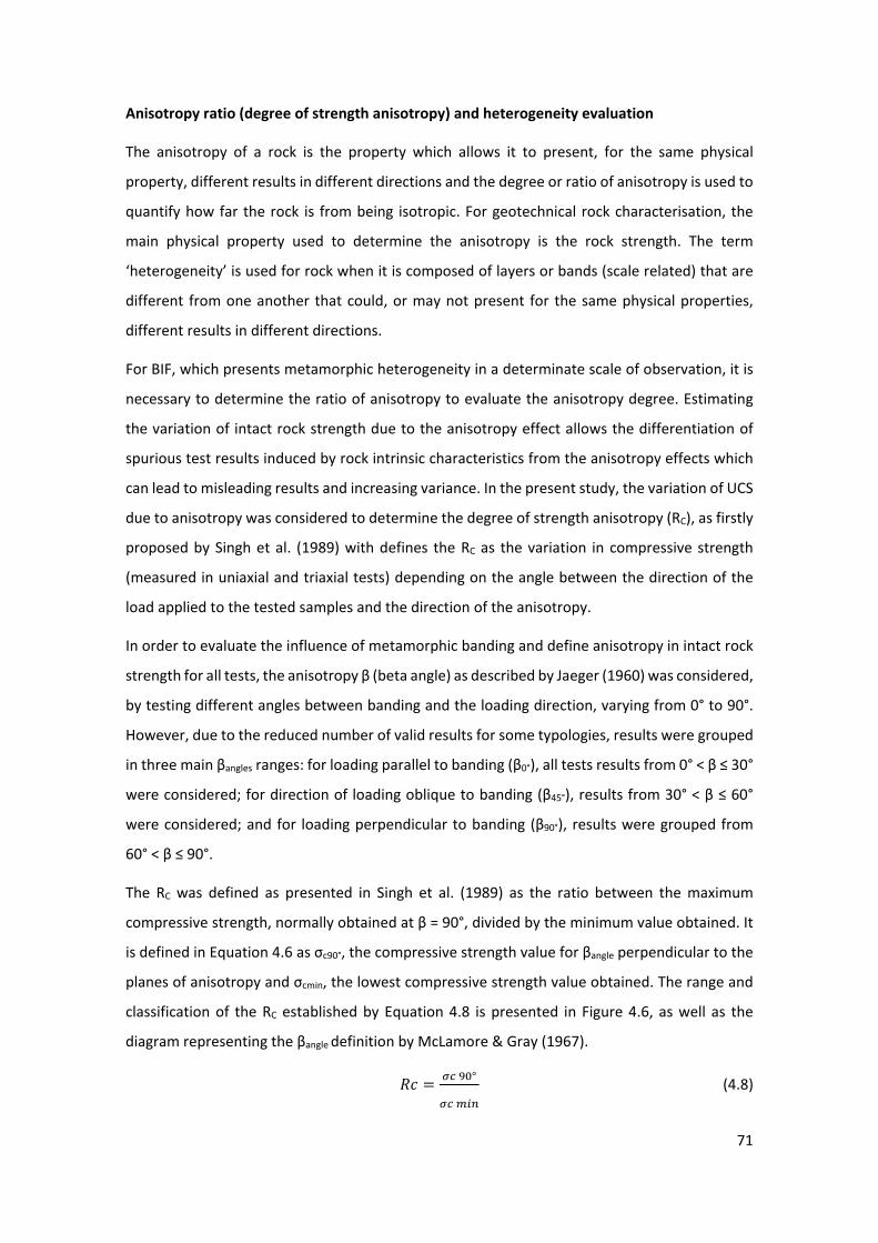
71
Anisotropy ratio (degree of strength anisotropy) and heterogeneity evaluation
The anisotropy of a rock is the property which allows it to present, for the same physical
property, different results in different directions and the degree or ratio of anisotropy is used to
quantify how far the rock is from being isotropic. For geotechnical rock characterisation, the
main physical property used to determine the anisotropy is the rock strength. The term
‘heterogeneity’ is used for rock when it is composed of layers or bands (scale related) that are
different from one another that could, or may not present for the same physical properties,
different results in different directions.
For BIF, which presents metamorphic heterogeneity in a determinate scale of observation, it is
necessary to determine the ratio of anisotropy to evaluate the anisotropy degree. Estimating
the variation of intact rock strength due to the anisotropy effect allows the differentiation of
spurious test results induced by rock intrinsic characteristics from the anisotropy effects which
can lead to misleading results and increasing variance. In the present study, the variation of UCS
due to anisotropy was considered to determine the degree of strength anisotropy (RC), as firstly
proposed by Singh et al. (1989) with defines the RC as the variation in compressive strength
(measured in uniaxial and triaxial tests) depending on the angle between the direction of the
load applied to the tested samples and the direction of the anisotropy.
In order to evaluate the influence of metamorphic banding and define anisotropy in intact rock
strength for all tests, the anisotropy β (beta angle) as described by Jaeger (1960) was considered,
by testing different angles between banding and the loading direction, varying from 0° to 90°.
However, due to the reduced number of valid results for some typologies, results were grouped
in three main βangles ranges: for loading parallel to banding (β0°), all tests results from 0° < β ≤ 30°
were considered; for direction of loading oblique to banding (β45°), results from 30° < β ≤ 60°
were considered; and for loading perpendicular to banding (β90°), results were grouped from
60° < β ≤ 90°.
The RC was defined as presented in Singh et al. (1989) as the ratio between the maximum
compressive strength, normally obtained at β = 90°, divided by the minimum value obtained. It
is defined in Equation 4.6 as σc90°, the compressive strength value for βangle perpendicular to the
planes of anisotropy and σcmin, the lowest compressive strength value obtained. The range and
classification of the RC established by Equation 4.8 is presented in Figure 4.6, as well as the
diagram representing the βangle definition by McLamore & Gray (1967).
𝑅𝑅𝑅𝑅 = 𝜎𝜎𝜎𝜎 90°
𝜎𝜎𝜎𝜎 𝑚𝑚𝑚𝑚𝑚𝑚 (4.8)
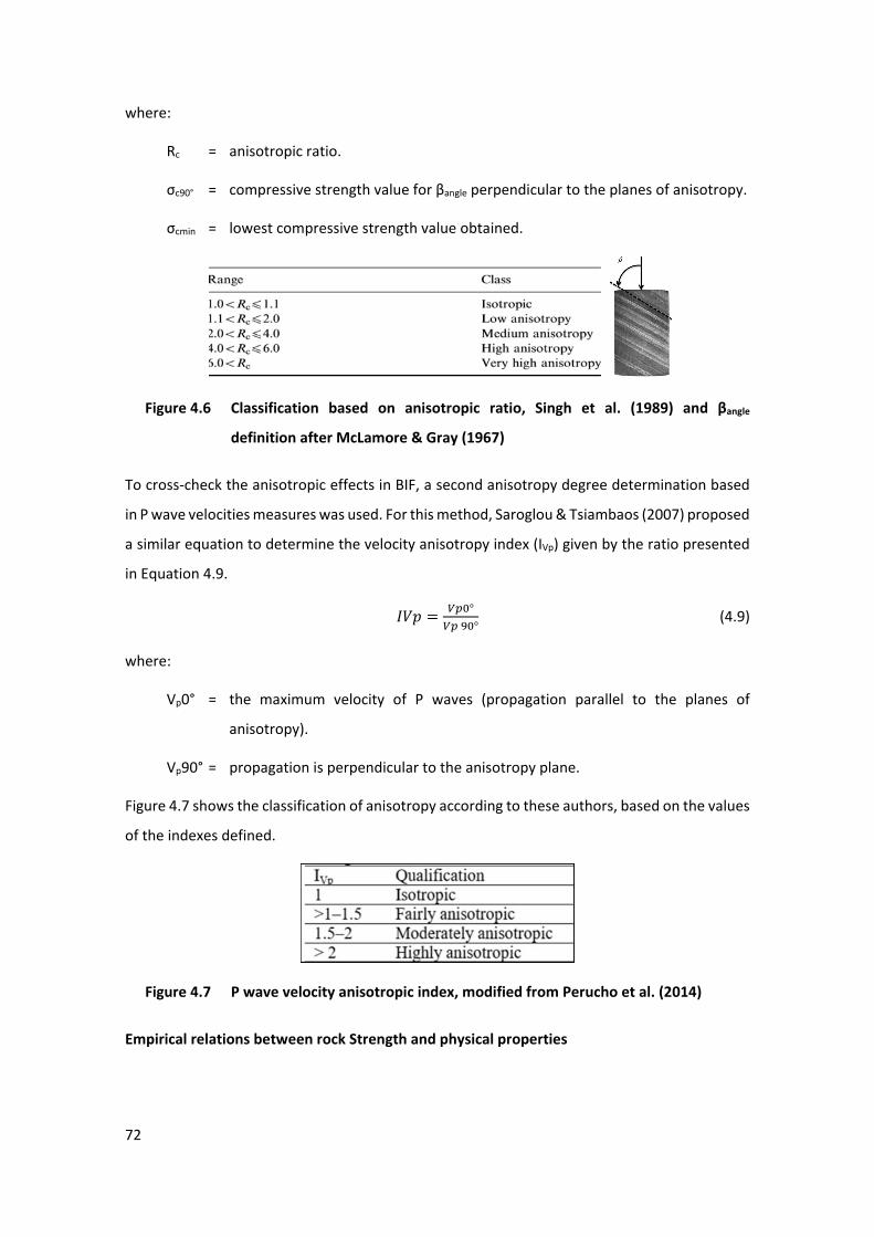
72
where:
Rc = anisotropic ratio.
σc90° = compressive strength value for βangle perpendicular to the planes of anisotropy.
σcmin = lowest compressive strength value obtained.
18 Figure 4.6 Classification based on anisotropic ratio, Singh et al. (1989) and βangle
definition after McLamore & Gray (1967)
To cross-check the anisotropic effects in BIF, a second anisotropy degree determination based
in P wave velocities measures was used. For this method, Saroglou & Tsiambaos (2007) proposed
a similar equation to determine the velocity anisotropy index (IVp) given by the ratio presented
in Equation 4.9.
𝐼𝐼𝐼𝐼𝐼𝐼 = 𝑉𝑉𝑉𝑉0°𝑉𝑉𝑉𝑉 90°
(4.9)
where:
Vp0° = the maximum velocity of P waves (propagation parallel to the planes of
anisotropy).
Vp90° = propagation is perpendicular to the anisotropy plane.
Figure 4.7 shows the classification of anisotropy according to these authors, based on the values
of the indexes defined.
19 Figure 4.7 P wave velocity anisotropic index, modified from Perucho et al. (2014)
Empirical relations between rock Strength and physical properties
73
practical approach in engineering problems. The use of such relations is often the only way to
estimate strength, due to the absence of cores for laboratory tests or even the lack of tests. The
basis for such relationships is the fact that many of the factors that affect rock strength also
affect other physical and mechanical parameters such as wave velocity, elastic module, bulk
density, Poisson’s ratio, and porosity for example.
To evaluate this relationship for two sets of data which are strongly linked together and to be
able to measure and determine the relationship between two variables, an adequate coefficient
of determination, which describes the strength and the direction of the variable’s correlations,
must be determined. In addition, these correlations could be expressed by linear or not linear
regression methods due to the nature of evaluating variables. The correlation coefficient has
been calculated by using the best fitting approach using automatic procedures through several
attempts on the dataset.
For Butel et al. (2014), the quality of the correlation is determined by the values of the coefficient
of determination (R2), the size of the dataset, and the visual fit of the regression curve. An
adjusted curve is defined as the curve that best evaluates the dispersion of the dataset and
defines the adjusted equation that gives the proportion of the variance in the independent
variables. In other words, the R2is a measure of how well a regression curve matches a set of
data for an evaluated dataset. It could also be interpreted as the adjusted model of observed
effects between two dependent variables. The strength of the correlation is defined as 0 to 0.29
(little if any correlation), 0.3 to 0.49 (low), 0.5 to 0.69 (moderate), 0.7 to 0.89 (high) and 0.9 to
1.0 (very high correlation) as presented by Asuero et al. (2006).
During correlation evaluations analysis, several adjusted fitting curves (e.g. linear, exponential,
and potential) were tested. The exponential adjustment curve proved to be the most suitable
for the available dataset and even when some correlation proves to be better for linear or
potential regressions (e.g. the correlation ratio obtained were not significantly different from
the exponential values).
Due to the material characteristics and the lack of references for studied rock types, a
correlation ratio equal or superior to 0.50 (moderate) was considered adequate.
4.4.1 Laboratory tests
For hard, fresh to slightly weathered lithotypes, UCS (σci) and modulus of elasticity (Estat and νstat)
were determined. P wave velocity (Vp) was used to evaluate the integrity of the samples. Bulk
74
density (ρb) results and thin sections descriptions were used to correlate and define geological
and physical properties such as total porosity, anisotropy, mineralogy, and microfabric.
For laboratory tests, selected rock samples from surface outcrops and drill cores were
subsampled, rectified, and prepared according to each standard, as detailed below.
All laboratory tests results are presented at Appendices III and IV.
Uniaxial compressive or unconfined compressive strength tests
The first set of UCS tests (total of 93 samples) was undertaken at an Australian laboratory in
accordance with the ASTM D2938-95 (ASTM 2002) standard procedures. For all analysis,
samples (cylindrical plugs) were obtained from the original 77.8 mm diamond drill core,
subsampled in 20 mm diameter, with lengths varying from 40 mm to 50 mm, prepared according
to ASTM D4543-01 (ASTM 2001). Sub-sampling allowed for evaluation of possible anisotropy not
available when using full size core. For a better axial and lateral strain determination,
simultaneous measurements were undertaken using, in general, two pairs of diametral strain
gauges and up to four axial gauges and four lateral gauges. All samples were subjected to a
constant loading rate of 7 MPa/min or 9 MPa/min.
The second set of UCS tests (total of 62 samples) was undertaken at a Brazilian laboratory. These
tests were also performed in accordance with ASTM D 2938-95 (ASMT 2002). For all tests,
cylindrical samples were obtained from the original diamond drill core of 50 mm to 76 mm
diameter, with lengths varying from 110 mm to 205 mm, prepared in accordance with ASTM
D4543-01 (ASTM 2001). Axial and lateral measurements were obtained by double dial indicator
gauges, and the strain was calculated by taking the average value for each direction. It is noted
that dial indicator gauges were less efficient than strain gauges. For this reason, some bias was
expected for this set of results.
Considering both sets, a total of 155 samples were tested. The average strain was calculated by
taking the average of all strain readings, and Young’s modulus and Poisson’s ratio were
calculated.
The axial (ξax) and radial (ξrad) deformation curves obtained from UCS testing are a function of
the compressive stresses applied and represents the typical deformational behaviour of the rock
in the absence of loading to the ultimate stress (σaxial) or peak stress, providing a good
description of the nonlinear behaviour model of rocky materials. The static elastic coefficient,
or Young’s modulus (Estat), was determined for that stretch of the axial curve (or stress range)
where the rock exhibits elastic behaviour (linear portion of the curve).
75
In this chapter, the tangent modulus (Estat) was determined by the slope of the line that tangents
the regression curve at a given point corresponding to a fixed percentage of the ultimate or peak
stress (𝜎𝜎u), normally 50%. The Poisson's ratio (νstat) which correlates the axial and radial
deformation, was obtained in the stretches of the curve corresponding to the observed limits
for obtaining the deformability moduli.
Due to the difficulty in preparing reliable samples during the extraction process, some types
presented reduced numbers of proper samples, specially FDI at β0°, HHE at β90°, and β45°.This
reduced number of tests could influence evaluations and produce bias in the interpretation.
For all samples prepared and tested with diameter sizes different from 50 mm, the results were
converted to d50mm based on the empirical correlation proposed by Hoek & Brown (1980).
Equation 4.10 shows the referenced methodology where σcd is the UCS of a sample with
diameter, ‘d’; and σC50 is the UCS of a 50 mm diameter sample. It is generally accepted that there
is a significant reduction in strength with increasing specimen size.
𝜎𝜎cd = 𝜎𝜎𝑅𝑅50 � 𝑑𝑑50�0.18
(4.10)
where:
σcd = UCS of a sample with diameter.
σC50 = UCS of a 50 mm diameter sample.
d = samples diameter.
P wave velocity
For the second UCS test set (62 tests), the primary sonic wave velocity (Vp) experiments were
undertaken according to ASTM D2845-08 (ASTM 2018). The experiments were performed using
equipment that calculates the velocity propagation of compressional waves (the P wave), by
measuring its time of transit through the axial length of the sample. Once the length of the
sample is known, as well as the time of transit of elastic waves, velocities are obtained from the
ratio of these parameters. Although P wave velocities were measured in all UCS tests, the lack
of S wave velocity made it impossible to obtain the dynamic elastic parameters.
Bulk density
In this chapter, bulk density was determined for all UCS tests (n = 155) according to the ratio
between the total dry mass and total volume. Bulk density of each specimen is calculated
according to IAS 1289.6.4.1 (AS 2016) for Australian laboratory and ABNT NBR 6508 (ABNT 1989)
for Brazilian laboratory, using Equation 4.11:
76
ρb = M/V (4.11)
where:
ρb = bulk density (kg/m3)
M = mass of the specimen measured prior to testing (kg)
V = volume (m3) of the specimen, calculated from dimensions measured during
sample preparation.
Petrographic thin sections description
Petrographic thin sections were prepared perpendicular and parallel to the bedding plane to
evaluate visual total porosity (Øb), crystal and pore size, crystal shape and distribution,
mineralogy and pore percentage, and fabric. This information was used to confirm the presence
of microscale features already observed on a macroscale, such as heterogeneity, anisotropy,
total porosity, and mineral distribution.
A total of 23 fresh BIF thin sections were prepared and evaluated. The sections were studied
under a research grant, supervised by the lead author, and presented in Horta & Costa (2016).
It should be noted that variations in crystal and pore size and percentage are closely correlated
with the geological settings of the sample site and the evaluation presented here is restricted to
the 23 thin sections from studied sites and reference review available.
4.5 RESULTS
4.5.1 Mineralogical and fabric overview
The mineralogical ensemble, textural characteristic (rock fabric) and visual total porosity are
important information used to define the anisotropic behaviour and geomechanical properties
for the BIF. The analyses for FQI, FDI and FAI were supported using field investigations and were
used in conjunction with microscopic evaluations from Horta & Costa (2016), while for HHE, as
there is a vast reference available related to its fabric and mineralogical composition, reference
the studies by Rosière et al. (1996 and 2001), Varajão et al. (2002) and Spier et al. (2003) were
used.
As suggested by Baars & Rosière (1994) and Rosière et al. (2001), the BIF fabric at the western
side of the Iron Quadrangle can be separated into three major domains: a subhedral to euhedral
crystals domain, with an overall granoblastic fabric, defined as the most common type and
considered to represent post-tectonic partial recrystallisation; a euhedral domain of locally
77
tabular-shaped or very elongated specularite platelets, preferred oriented, defining a secondary
schistosity induced by shearing and a high stress domain; and a locally brecciaed fabric domain,
that can occur induced by tectonical or physical collapse zones.
Such domains reflect distinct micro characteristics that are not always noticed on the
macroscale. They are associated with the main three geological settings that influence the
geomechanical and anisotropic behaviour: a post tectonical domain (weathering) characterised
by the leaching of the boundary contact; tectonical high stress zones describing oriented mineral
assemblage; and brecciated zone (weathering or tectonical) with porous level oriented or not.
Table 4.1 shows summary results for 23 thin sections presenting the name and percentage of
the main constituent minerals, and maximum and minimum crystal size (between brackets).
Also presented the percentage, and maximum and minimum size (between brackets) of pores
for three types of measures. As known, intragranular pores correspond with the percentage of
pores inside crystals that can or cannot be interconnected. Intergranular pores correspond with
porosity between crystals and are generally interconnected. Secondary pores refer to fracture
pore percentage. Total porosity is the sum of the three pore percentages and is considered the
maximum total percentage. For Øb in brackets, the minimum value did not consider the
secondary pores (intact rock) and for maximum value, the secondary pore is included.
Hematitites, as mentioned, were not evaluated because there is vast reference related to its
fabric, mineralogical composition, and crystal size. This information is presented in Table 4.1
obtained from Rosière et al. (1996 and 2001), Varajão et al. (2002) and Spier et al. (2003).
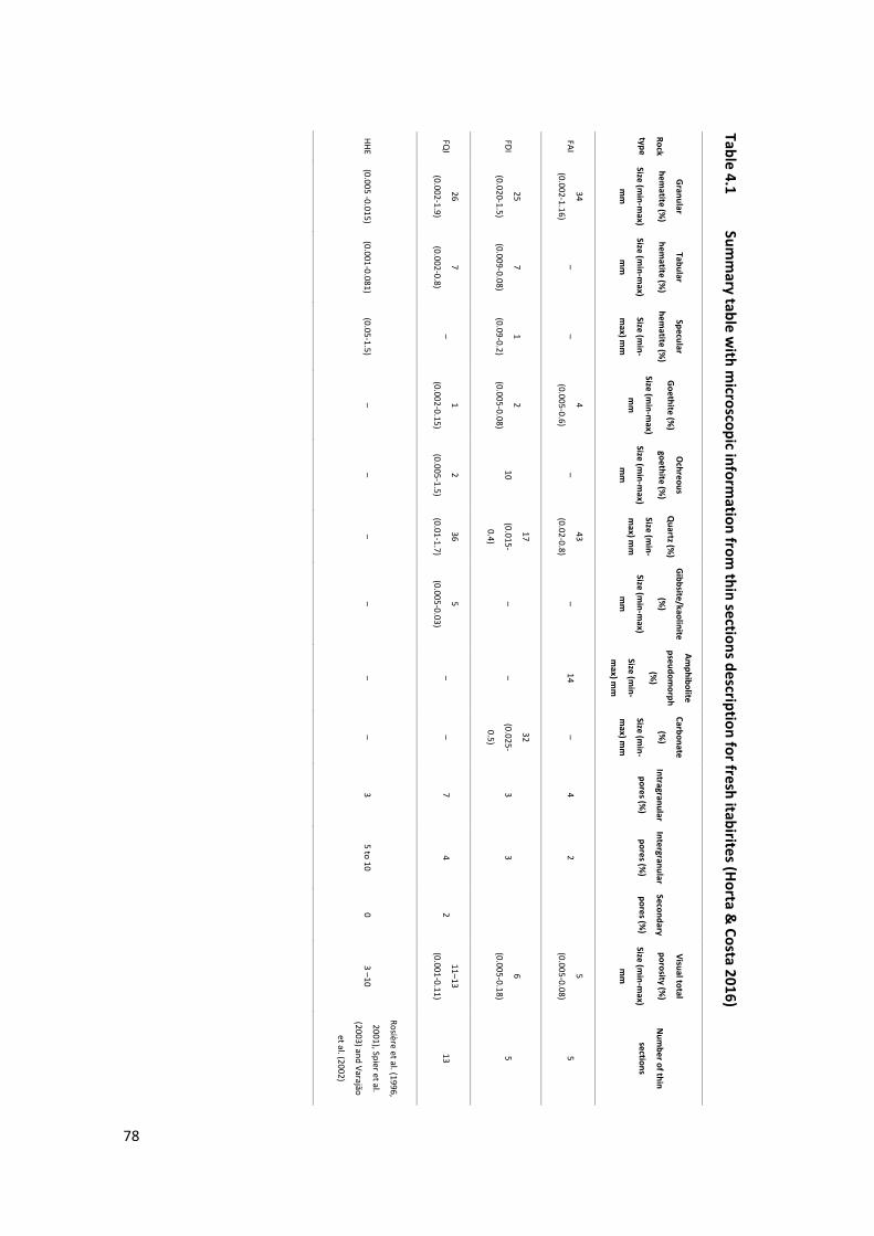
1Table 4.1 Sum
mary table w
ith microscopic inform
ation from thin sections description for fresh itabirites (H
orta & Costa 2016)
Rock
type
Granular
hematite (%
)
Size (min-m
ax)
mm
Tabular
hematite (%
)
Size (min-m
ax)
mm
Specular
hematite (%
)
Size (min-
max) m
m
Goethite (%
)
Size (min-m
ax)
mm
Ochreous
goethite (%)
Size (min-m
ax)
mm
Quartz (%
)
Size (min-
max) m
m
Gibbsite/kaolinite
(%)
Size (min-m
ax)
mm
Amphibolite
pseudomorph
(%)
Size (min-
max) m
m
Carbonate
(%)
Size (min-
max) m
m
Intragranular
pores (%)
Intergranular
pores (%)
Secondary
pores (%)
Visual total
porosity (%)
Size (min-m
ax)
mm
Num
ber of thin
sections
FAI 34
(0.002-1.16) –
– 4
(0.005-0.6) –
43
(0.02-0.8) –
14–
42
5
(0.005-0.08) 5
FDI 25
(0.020-1.5)
7
(0.009-0.08)
1
(0.09-0.2)
2
(0.005-0.08) 10
17
(0.015-
0.4)
– –
32
(0.025-
0.5)
3 3
6
(0.005-0.18) 5
FQI
26
(0.002-1.9)
7
(0.002-0.8) –
1
(0.002-0.15)
2
(0.005-1.5)
36
(0.01-1.7)
5
(0.005-0.03) –
– 7
4 2
11–13
(0.001-0.11) 13
HHE (0.005 -0.015)
(0.001-0.081) (0.05-1.5)
– –
– –
– –
3 5 to 10
0 3 –10
Rosière et al. (1996,
2001), Spier et al.
(2003) and Varajão
et al. (2002)
78
79
In general, the analyses of these thin sections indicated three main characteristics of pervasive
fabric responsible for inducing penetrative planes that could represent heterogeneity and result
in rock anisotropy:
• Band boundary contacts between layers with different mineral compositions, defining
the compositional metamorphic banding, mainly quartz for FQI, FAI, and carbonates
for FDI. This characteristic is not observed for HHE as it is a monomineralic rock.
• Planar or granular minerals oriented in one direction (mineral orientation), defined by
tabular hematite and recrystalised quartz and carbonate crystals.
• Oriented porous layers (pore orientation), defined by intergranular pores oriented
align the metamorphic banding (band boundary and mineral orientation) or along
discontinuities. This characteristic defines the metamorphic banding for HHE.
A summarised description of each lithotype is presented below:
Fresh quartzitic itabirite
Fresh quartzitic itabirite mineralogy is marked by granular quartz and hematite, tabular
hematite, and goethite. Ochreous goethite, kaolinite, and gibbsite occur as accessory minerals.
The goethite appears as small crystals in quartz rich bands, with anhedral shapes and can also
occur filling pores. Bands of quartz have higher Øb = 20%, mainly resulting from intergranular
pores. In these bands, microplates of hematite occur in larger quantities and the visual total
porosity is slightly smaller.
Bands of hematite present with lower Øb = 7% but the presence of lobed crystals, tabular
hematite crystals larger than 0.80 mm and granular hematites larger than 1.3 mm. In some
bands the Øb can reach 30%. Hematite crystals lower than 1.3 mm were considered part of the
banding itself.
In general, FQI presented higher Øb ranging from 11% to 13%, compared with another fresh BIF.
This difference can be attributed to the presence of slightly weathered degree (W1) thin sections
that could influence the results.
Fresh amphibolitic itabirite
The mineralogy of fresh amphibolitic itabirite is mainly defined by quartz, hematite, goethite as
pseudomorph of amphibolite, and ochreous goethite. The pseudomorphs of amphibolite are
generally altered to goethite and only occur in some thin sections. Goethite usually occurs with
anhedral shape between quartz crystals as a cement, but also in smaller percentages as crystals.
80
Quartz bands are well preserved and large hematite crystals (1.1 mm) were interpreted as being
part of the preserved hematite band. Hematite bands present lower total porosity and the limits
between quartz and hematite bands are not very clear due to the pore distribution and lower
concentration in the boundaries as observed in FQI. Ochreous goethite and gibbsite are also
present, and kaolinite appear as accessory minerals. All the samples present low Øb = 5%.
Fresh dolomitic itabirite
The mineralogy of fresh dolomitic itabirite is defined by hematite, iron dolomite, quartz, and
goethite. Granular hematite predominates, although its size (0.90 mm) decreases to 0.02 mm
when higher quantities of ankerite and siderite dolomites occur. These minerals occur
interlayered with hematite bands as granoblastic crystals, as well as a cement in the filling spaces
between crystals. Goethite occurs as a cement filling spaces in between crystals of hematite and
iron dolomite (minor). Quartz is present in bands and exhibits oriented crystals and sub-crystals.
FDI presents low Øb = 6%. Bands of hematite also present some percentage of iron dolomites
and are characterised by relatively lower visual total porosity. In this band, hematite occurs as
granular and/or tabular crystals and iron dolomites as a matrix with very fine crystals. Talc,
carbonate and goethite also occur as accessory minerals.
Hard hematitite
As already presented in Section 4.3.2.
4.5.2 BIF, heterogeneity and anisotropy
Based on geological macro and micro features, it is expected that the heterogeneity promoted
by typical compositional metamorphic banding in BIF will be the main characteristic responsible
for an anisotropic behaviour. Analysis conducted during this research showed at least three
different types of either repetitive or discrete surfaces of disruption that could create an
anisotropic intact rock strength for fresh BIF.
Analyses conducted in Section 4.1 found three main characteristics of pervasive fabric that could
be responsible for inducing penetrative planes representing heterogeneity and result in rock
anisotropy: boundary contacts between layers with different mineral composition, defining the
compositional metamorphic banding; planar or granular minerals oriented according to one
direction (mineral orientation); and oriented porous levels (pore orientation).
The heterogeneity observed in itabirites is different from that observed in hematitites. The
differences will be presented in the following sections. Both satisfy the heterogeneity
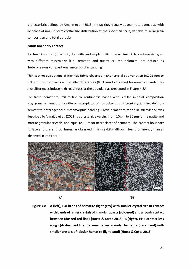
81
characteristic defined by Amann et al. (2013) in that they visually appear heterogeneous, with
evidence of non-uniform crystal size distribution at the specimen scale, variable mineral grain
composition and total porosity.
Bands boundary contact
For fresh itabirites (quartzitic, dolomitic and amphibolitic), the millimetric to centimetric layers
with different mineralogy (e.g. hematite and quartz or iron dolomite) are defined as
’heterogenous compositional metamorphic banding’.
Thin section evaluations of itabiritic fabric observed higher crystal size variation (0.002 mm to
1.9 mm) for iron bands and smaller differences (0.01 mm to 1.7 mm) for non-iron bands. This
size differences induce high roughness at the boundary as presented in Figure 4.8A.
For fresh hematitite, millimetric to centimetric bands with similar mineral composition
(e.g. granular hematite, martite or microplates of hematite) but different crystal sizes define a
hematitite heterogeneous metamorphic banding. Fresh hematitite fabric in microscope was
described by Varajão et al. (2002), as crystal size varying from 10 μm to 30 μm for hematite and
martite granular crystals, and equal to 1 μm for microplates of hematite. The contact boundary
surface also present roughness, as observed in Figure 4.8B, although less prominently than as
observed in itabirites.
(A) (B)
20 Figure 4.8 A (left), FQI bands of hematite (light grey) with smaller crystal size in contact
with bands of larger crystals of granular quartz (coloured) and a rough contact
between (dashed red line) (Horta & Costa 2016). B (right), HHE contact less
rough (dashed red line) between larger granular hematite (dark band) with
smaller crystals of tabular hematite (light band) (Horta & Costa 2016)
500μm
A B
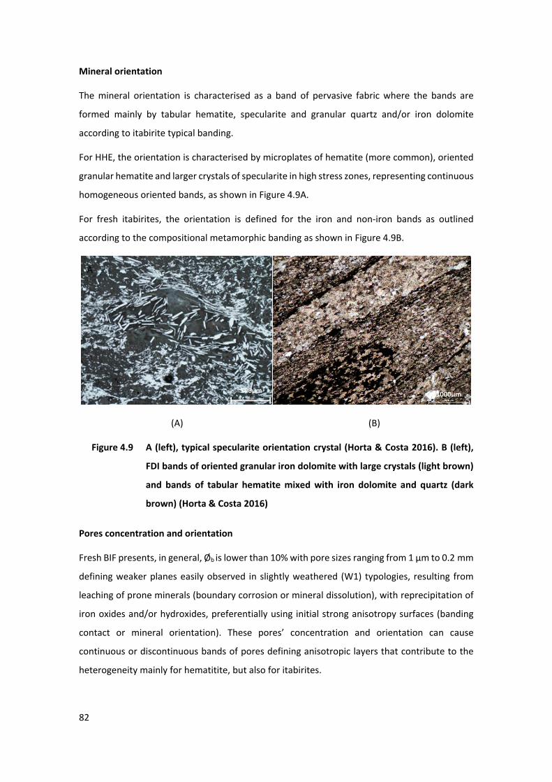
82
Mineral orientation
The mineral orientation is characterised as a band of pervasive fabric where the bands are
formed mainly by tabular hematite, specularite and granular quartz and/or iron dolomite
according to itabirite typical banding.
For HHE, the orientation is characterised by microplates of hematite (more common), oriented
granular hematite and larger crystals of specularite in high stress zones, representing continuous
homogeneous oriented bands, as shown in Figure 4.9A.
For fresh itabirites, the orientation is defined for the iron and non-iron bands as outlined
according to the compositional metamorphic banding as shown in Figure 4.9B.
(A) (B)
21 Figure 4.9 A (left), typical specularite orientation crystal (Horta & Costa 2016). B (left),
FDI bands of oriented granular iron dolomite with large crystals (light brown)
and bands of tabular hematite mixed with iron dolomite and quartz (dark
brown) (Horta & Costa 2016)
Pores concentration and orientation
Fresh BIF presents, in general, Øb is lower than 10% with pore sizes ranging from 1 μm to 0.2 mm
defining weaker planes easily observed in slightly weathered (W1) typologies, resulting from
leaching of prone minerals (boundary corrosion or mineral dissolution), with reprecipitation of
iron oxides and/or hydroxides, preferentially using initial strong anisotropy surfaces (banding
contact or mineral orientation). These pores’ concentration and orientation can cause
continuous or discontinuous bands of pores defining anisotropic layers that contribute to the
heterogeneity mainly for hematitite, but also for itabirites.
500μm
A B
1000μm
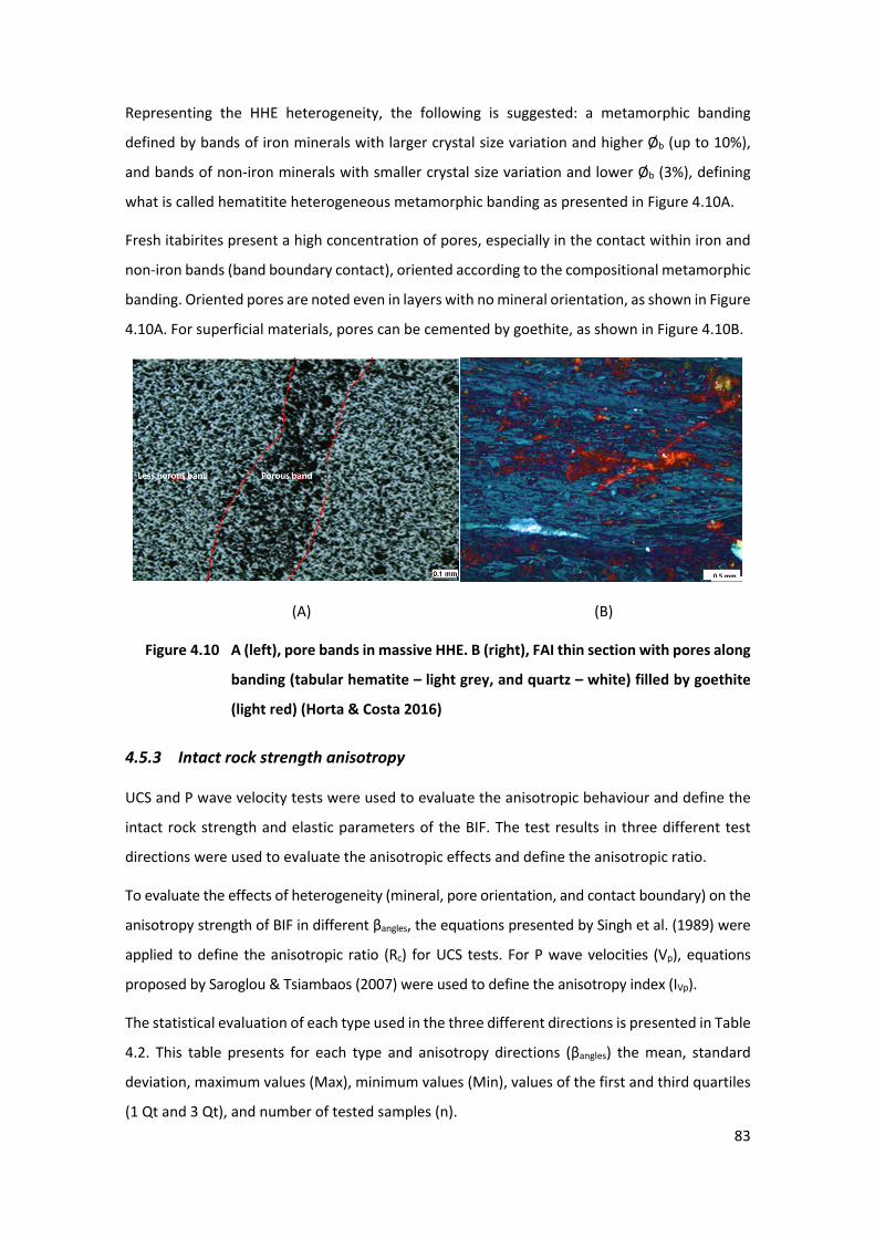
83
Representing the HHE heterogeneity, the following is suggested: a metamorphic banding
defined by bands of iron minerals with larger crystal size variation and higher Øb (up to 10%),
and bands of non-iron minerals with smaller crystal size variation and lower Øb (3%), defining
what is called hematitite heterogeneous metamorphic banding as presented in Figure 4.10A.
Fresh itabirites present a high concentration of pores, especially in the contact within iron and
non-iron bands (band boundary contact), oriented according to the compositional metamorphic
banding. Oriented pores are noted even in layers with no mineral orientation, as shown in Figure
4.10A. For superficial materials, pores can be cemented by goethite, as shown in Figure 4.10B.
(A) (B)
22 Figure 4.10 A (left), pore bands in massive HHE. B (right), FAI thin section with pores along
banding (tabular hematite – light grey, and quartz – white) filled by goethite
(light red) (Horta & Costa 2016)
4.5.3 Intact rock strength anisotropy
UCS and P wave velocity tests were used to evaluate the anisotropic behaviour and define the
intact rock strength and elastic parameters of the BIF. The test results in three different test
directions were used to evaluate the anisotropic effects and define the anisotropic ratio.
To evaluate the effects of heterogeneity (mineral, pore orientation, and contact boundary) on the
anisotropy strength of BIF in different βangles, the equations presented by Singh et al. (1989) were
applied to define the anisotropic ratio (Rc) for UCS tests. For P wave velocities (Vp), equations
proposed by Saroglou & Tsiambaos (2007) were used to define the anisotropy index (IVp).
The statistical evaluation of each type used in the three different directions is presented in Table
4.2. This table presents for each type and anisotropy directions (βangles) the mean, standard
deviation, maximum values (Max), minimum values (Min), values of the first and third quartiles
(1 Qt and 3 Qt), and number of tested samples (n).
0.5 mm
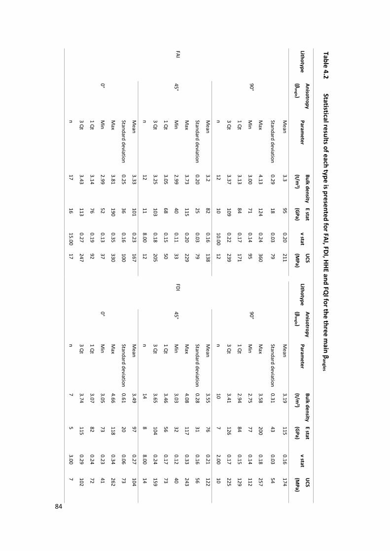
2 Table 4.2 Statistical results of each type is presented for FAI, FDI, HH
E and FQI for the three m
ain βangles
Lithotype Anisotropy
(βangle )
Parameter
Bulk density
(t/m3)
E stat
(GPa)
v stat U
CS
(MPa)
Lithotype Anisotropy
(βangle )
Parameter
Bulk density
(t/m3)
E stat
(GPa)
v stat U
CS
(MPa)
FAI
90°
Mean
3.3 95
0.20 211
FDI
90°
Mean
3.19 115
0.16 174
Standard deviation 0.29
18 0.03
79 Standard deviation
0.31 43
0.03 54
Max
4.13 124
0.24 360
Max
3.58 200
0.18 257
Min
3.00 71
0.14 95
Min
2.75 77
0.14 112
1 Qt
3.13 84
0.17 171
1 Qt
2.94 84
0.15 129
3 Qt
3.37 109
0.22 239
3 Qt
3.41 126
0.17 225
n 12
10 10.00
12 n
10 7
2.00 10
45°
Mean
3.2 82
0.16 138
45°
Mean
3.55 76
0.21 122
Standard deviation 0.20
25 0.03
79 Standard deviation
0.28 31
0.16 56
Max
3.73 115
0.20 229
Max
4.08 117
0.33 243
Min
2.99 40
0.11 33
Min
3.03 32
0.12 40
1 Qt
3.05 68
0.15 50
1 Qt
3.46 56
0.17 73
3 Qt
3.25 103
0.18 205
3 Qt
3.65 104
0.24 159
n 12
11 8.00
12 n
14 8
8.00 14
0°
Mean
3.33 101
0.23 167
0°
Mean
3.49 97
0.27 104
Standard deviation 0.25
36 0.16
100 Standard deviation
0.61 20
0.06 73
Max
3.81 190
0.35 330
Max
4.66 118
0.34 262
Min
2.99 52
0.13 37
Min
3.05 73
0.23 41
1 Qt
3.14 76
0.19 92
1 Qt
3.07 82
0.24 72
3 Qt
3.43 113
0.27 247
3 Qt
3.74 115
0.29 102
n 17
16 15.00
17 n
7 5
3.00 7
84
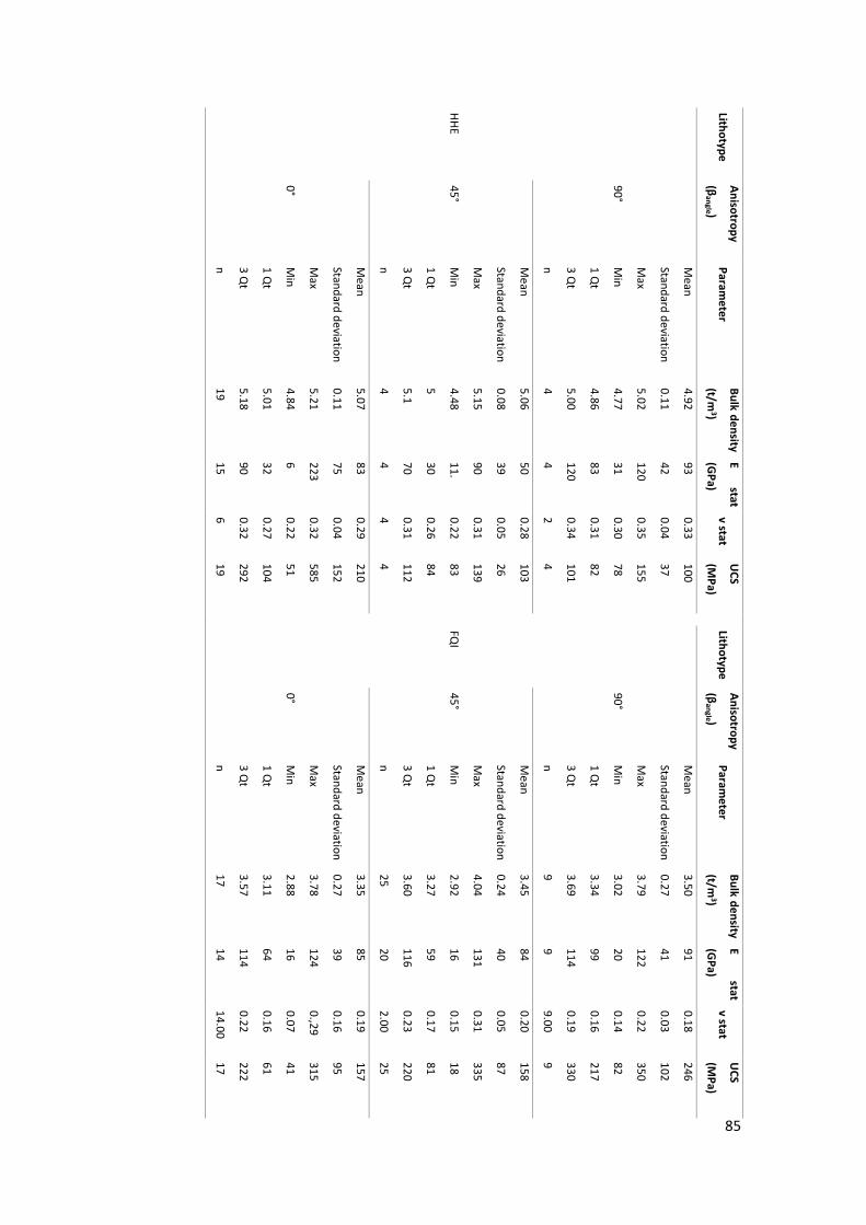
Lithotype Anisotropy
(βangle )
Parameter
Bulk density
(t/m3)
E stat
(GPa)
v stat U
CS
(MPa)
Lithotype Anisotropy
(βangle )
Parameter
Bulk density
(t/m3)
E stat
(GPa)
v stat U
CS
(MPa)
HHE
90°
Mean
4.92 93
0.33 100
FQI
90°
Mean
3.50 91
0.18 246
Standard deviation 0.11
42 0.04
37 Standard deviation
0.27 41
0.03 102
Max
5.02 120
0.35 155
Max
3.79 122
0.22 350
Min
4.77 31
0.30 78
Min
3.02 20
0.14 82
1 Qt
4.86 83
0.31 82
1 Qt
3.34 99
0.16 217
3 Qt
5.00 120
0.34 101
3 Qt
3.69 114
0.19 330
n 4
4 2
4 n
9 9
9.00 9
45°
Mean
5.06 50
0.28 103
45°
Mean
3.45 84
0.20 158
Standard deviation 0.08
39 0.05
26 Standard deviation
0.24 40
0.05 87
Max
5.15 90
0.31 139
Max
4.04 131
0.31 335
Min
4.48 11.
0.22 83
Min
2.92 16
0.15 18
1 Qt
5 30
0.26 84
1 Qt
3.27 59
0.17 81
3 Qt
5.1 70
0.31 112
3 Qt
3.60 116
0.23 220
n 4
4 4
4 n
25 20
2.00 25
0°
Mean
5.07 83
0.29 210
0°
Mean
3.35 85
0.19 157
Standard deviation 0.11
75 0.04
152 Standard deviation
0.27 39
0.16 95
Max
5.21 223
0.32 585
Max
3.78 124
0.,29 315
Min
4.84 6
0.22 51
Min
2.88 16
0.07 41
1 Qt
5.01 32
0.27 104
1 Qt
3.11 64
0.16 61
3 Qt
5.18 90
0.32 292
3 Qt
3.57 114
0.22 222
n 19
15 6
19 n
17 14
14.00 17
85
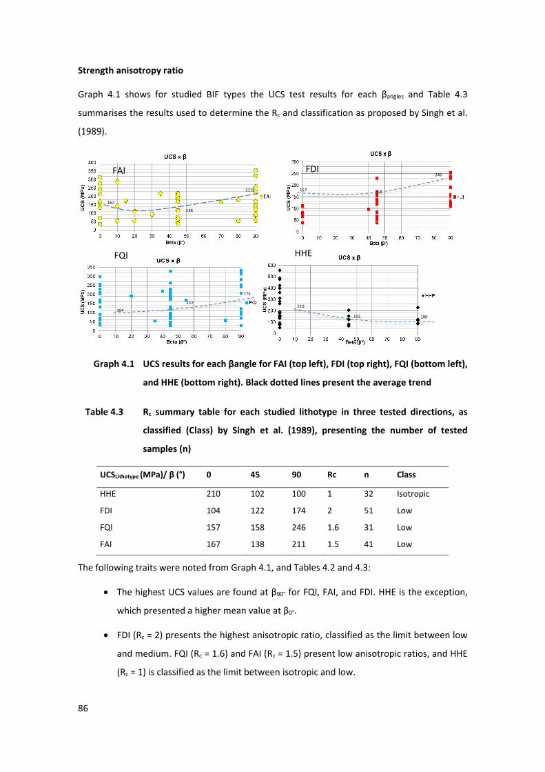
86
Strength anisotropy ratio
Graph 4.1 shows for studied BIF types the UCS test results for each βangles and Table 4.3
summarises the results used to determine the Rc and classification as proposed by Singh et al.
(1989).
0-1 Graph 4.1 UCS results for each βangle for FAI (top left), FDI (top right), FQI (bottom left),
and HHE (bottom right). Black dotted lines present the average trend
3 Table 4.3 Rc summary table for each studied lithotype in three tested directions, as
classified (Class) by Singh et al. (1989), presenting the number of tested
samples (n)
UCSLithotype (MPa)/ β (°) 0 45 90 Rc n Class
HHE 210 102 100 1 32 Isotropic
FDI 104 122 174 2 51 Low
FQI 157 158 246 1.6 31 Low
FAI 167 138 211 1.5 41 Low
The following traits were noted from Graph 4.1, and Tables 4.2 and 4.3:
• The highest UCS values are found at β90° for FQI, FAI, and FDI. HHE is the exception,
which presented a higher mean value at β0°.
• FDI (Rc = 2) presents the highest anisotropic ratio, classified as the limit between low
and medium. FQI (Rc = 1.6) and FAI (Rc = 1.5) present low anisotropic ratios, and HHE
(Rc = 1) is classified as the limit between isotropic and low.
157 158
246
104
122
174
210
102 100
167
138
2119
FAI
FQI HHE
FDI
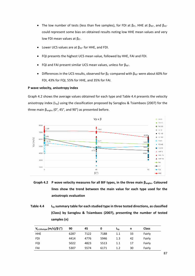
87
• The low number of tests (less than five samples), for FDI at β0°, HHE at β90°, and β45°
could represent some bias on obtained results noting low HHE mean values and very
low FDI mean values at β0°.
• Lower UCS values are at β45° for HHE, and FDI.
• FQI presents the highest UCS mean value, followed by HHE, FAI and FDI.
• FQI and FAI present similar UCS mean values, unless for β90°.
• Differences in the UCS results, observed for β0° compared with β90° were about 60% for
FDI, 43% for FQI, 55% for HHE, and 35% for FAI.
P wave velocity, anisotropy index
Graph 4.2 shows the average values obtained for each type and Table 4.4 presents the velocity
anisotropy index (IVp) using the classification proposed by Saroglou & Tsiambaos (2007) for the
three main βangles (0°, 45°, and 90°) as presented before.
0-2 Graph 4.2 P wave velocity measures for all BIF types, in the three main βangles. Coloured
lines show the trend between the main value for each type used for the
anisotropic evaluation
4 Table 4.4 IVp summary table for each studied type in three tested directions, as classified
(Class) by Saroglou & Tsiambaos (2007), presenting the number of tested
samples (n)
Vp Lithotype (m/s)/β (°) 90 45 0 IVp n Class
HHE 6287 7122 7188 1.1 33 Fairly FDI 4414 4776 5946 1.3 42 Fairly FQI 5022 4823 5513 1.1 17 Fairly FAI 5307 5574 6171 1.2 30 Fairly
88
The following traits were noted from Graph 4.2 and Table 4.4:
• The highest Vp values are found at β0° for all types. HHE presents the highest mean
value for all βangles.
• Lower Vp values for all BIF are at β90° except for FQI at β45°
• At β90°, HHE presents highest mean value followed by FAI, FQI and FDI. For β45°, FDI and
FQI presented similar results.
• FAI presents the highest values of Vp from all itabirites, and FDI shows the lowest mean
except for β0°
• Differences in Vp results, were obtained for β0° compared with β90° with about 26% for
FDI, 9% for FQI, 12% for HHE, and 14% for FAI.
• All types present fair degrees of anisotropy. This behaviour can be mainly induced by
the low total porosity and the fact that the pore bands are not continuous, as
previously reported in Section 4.5.2, allowing the P wave pulse to penetrate through
the sample portion not affected by pores, independent from anisotropy direction.
Considering this, the pulse will preferably travel through the portions with no pores
independent from the anisotropic direction or heterogeneity. The small difference
observed in different directions, mainly for itabirites, is associated with the band
mineral composition (heterogeneity). This heterogeneity contributed to the slightly
higher Ivp ratio obtained for FDI with most different mineral composition bands
compared to other itabirites.
Comparing the anisotropic ratio classification obtained for UCS and Vp in Tables 4.3 and 4.4, it is
possible to conclude that FDI is the type with highest anisotropic behaviour (Rc = 2 and IVp = 1.3),
HHE presents the lowest anisotropy degree (Rc = 1 and IVp = 1.1), and FQI (Rc = 1.6 and IVp = 1.1),
and FAI (Rc = 1.5 and IVp = 1.2), presenting similar anisotropy degree for both evaluations. In
general, HHE behaves like an isotropic material, and FAI, FQI and FDI behave similarly to low
anisotropic materials, however, FDI presents a slightly higher anisotropic ratio.
4.5.4 BIF characterisation of geomechanical properties and parameters
Results from Section 4.5.3 established that, in general, BIF are isotropic or have a low anisotropic
ratio. Based on this behaviour, geomechanical properties characterisations were evaluated for
seven different geomechanical parameter correlations (UCS and ρb, UCS and Vp, UCS and νstat,
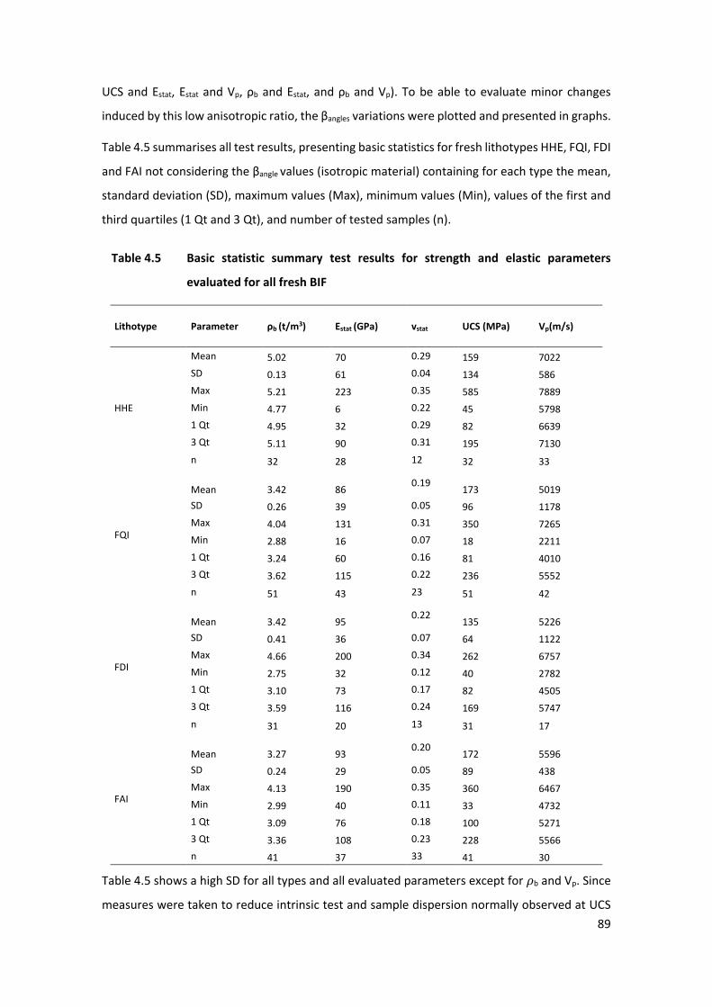
89
UCS and Estat, Estat and Vp, ρb and Estat, and ρb and Vp). To be able to evaluate minor changes
induced by this low anisotropic ratio, the βangles variations were plotted and presented in graphs.
Table 4.5 summarises all test results, presenting basic statistics for fresh lithotypes HHE, FQI, FDI
and FAI not considering the βangle values (isotropic material) containing for each type the mean,
standard deviation (SD), maximum values (Max), minimum values (Min), values of the first and
third quartiles (1 Qt and 3 Qt), and number of tested samples (n).
5 Table 4.5 Basic statistic summary test results for strength and elastic parameters
evaluated for all fresh BIF
Lithotype Parameter ρb (t/m3) Estat (GPa) vstat UCS (MPa) Vp(m/s)
HHE
Mean 5.02 70 0.29 159 7022 SD 0.13 61 0.04 134 586 Max 5.21 223 0.35 585 7889 Min 4.77 6 0.22 45 5798 1 Qt 4.95 32 0.29 82 6639 3 Qt 5.11 90 0.31 195 7130 n 32 28 12 32 33
FQI
Mean 3.42 86
0.19 173 5019
SD 0.26 39 0.05 96 1178 Max 4.04 131 0.31 350 7265 Min 2.88 16 0.07 18 2211 1 Qt 3.24 60 0.16 81 4010 3 Qt 3.62 115 0.22 236 5552 n 51 43 23 51 42
FDI
Mean 3.42 95
0.22 135 5226
SD 0.41 36 0.07 64 1122 Max 4.66 200 0.34 262 6757 Min 2.75 32 0.12 40 2782 1 Qt 3.10 73 0.17 82 4505 3 Qt 3.59 116 0.24 169 5747 n 31 20 13 31 17
FAI
Mean 3.27 93
0.20 172 5596
SD 0.24 29 0.05 89 438 Max 4.13 190 0.35 360 6467 Min 2.99 40 0.11 33 4732 1 Qt 3.09 76 0.18 100 5271 3 Qt 3.36 108 0.23 228 5566 n 41 37 33 41 30
Table 4.5 shows a high SD for all types and all evaluated parameters except for 𝜌𝜌b and Vp. Since
measures were taken to reduce intrinsic test and sample dispersion normally observed at UCS
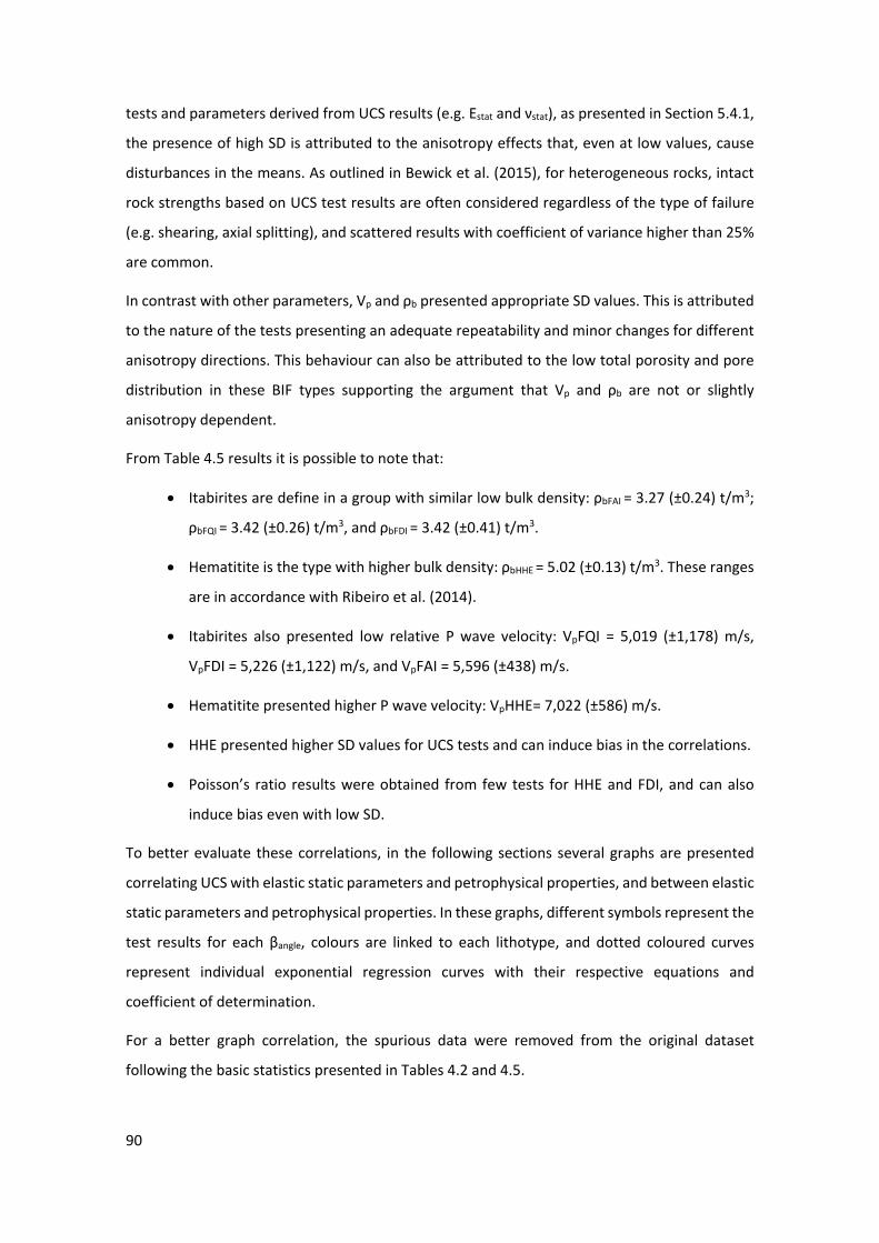
90
tests and parameters derived from UCS results (e.g. Estat and νstat), as presented in Section 5.4.1,
the presence of high SD is attributed to the anisotropy effects that, even at low values, cause
disturbances in the means. As outlined in Bewick et al. (2015), for heterogeneous rocks, intact
rock strengths based on UCS test results are often considered regardless of the type of failure
(e.g. shearing, axial splitting), and scattered results with coefficient of variance higher than 25%
are common.
In contrast with other parameters, Vp and ρb presented appropriate SD values. This is attributed
to the nature of the tests presenting an adequate repeatability and minor changes for different
anisotropy directions. This behaviour can also be attributed to the low total porosity and pore
distribution in these BIF types supporting the argument that Vp and ρb are not or slightly
anisotropy dependent.
From Table 4.5 results it is possible to note that:
• Itabirites are define in a group with similar low bulk density: ρbFAI = 3.27 (±0.24) t/m3;
ρbFQI = 3.42 (±0.26) t/m3, and ρbFDI = 3.42 (±0.41) t/m3.
• Hematitite is the type with higher bulk density: ρbHHE = 5.02 (±0.13) t/m3. These ranges
are in accordance with Ribeiro et al. (2014).
• Itabirites also presented low relative P wave velocity: VpFQI = 5,019 (±1,178) m/s,
VpFDI = 5,226 (±1,122) m/s, and VpFAI = 5,596 (±438) m/s.
• Hematitite presented higher P wave velocity: VpHHE= 7,022 (±586) m/s.
• HHE presented higher SD values for UCS tests and can induce bias in the correlations.
• Poisson’s ratio results were obtained from few tests for HHE and FDI, and can also
induce bias even with low SD.
To better evaluate these correlations, in the following sections several graphs are presented
correlating UCS with elastic static parameters and petrophysical properties, and between elastic
static parameters and petrophysical properties. In these graphs, different symbols represent the
test results for each βangle, colours are linked to each lithotype, and dotted coloured curves
represent individual exponential regression curves with their respective equations and
coefficient of determination.
For a better graph correlation, the spurious data were removed from the original dataset
following the basic statistics presented in Tables 4.2 and 4.5.
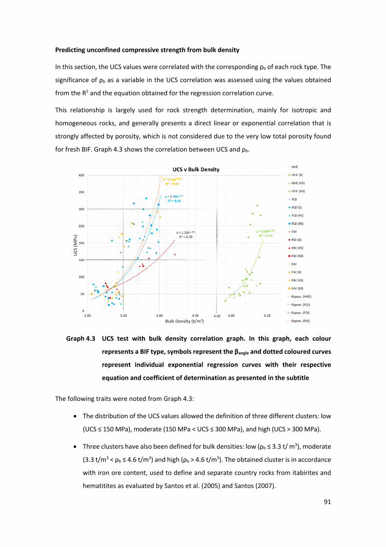
91
Predicting unconfined compressive strength from bulk density
In this section, the UCS values were correlated with the corresponding ρb of each rock type. The
significance of ρb as a variable in the UCS correlation was assessed using the values obtained
from the R2 and the equation obtained for the regression correlation curve.
This relationship is largely used for rock strength determination, mainly for isotropic and
homogeneous rocks, and generally presents a direct linear or exponential correlation that is
strongly affected by porosity, which is not considered due to the very low total porosity found
for fresh BIF. Graph 4.3 shows the correlation between UCS and ρb.
0-3 Graph 4.3 UCS test with bulk density correlation graph. In this graph, each colour
represents a BIF type, symbols represent the βangle and dotted coloured curves
represent individual exponential regression curves with their respective
equation and coefficient of determination as presented in the subtitle
The following traits were noted from Graph 4.3:
• The distribution of the UCS values allowed the definition of three different clusters: low
(UCS ≤ 150 MPa), moderate (150 MPa < UCS ≤ 300 MPa), and high (UCS > 300 MPa).
• Three clusters have also been defined for bulk densities: low (ρb ≤ 3.3 t/ m3), moderate
(3.3 t/m3 < ρb ≤ 4.6 t/m3) and high (ρb > 4.6 t/m3). The obtained cluster is in accordance
with iron ore content, used to define and separate country rocks from itabirites and
hematitites as evaluated by Santos et al. (2005) and Santos (2007).
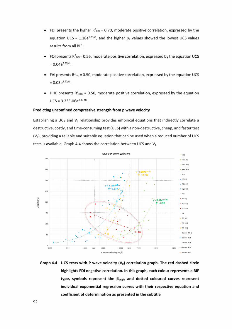
92
• FDI presents the higher R2FDI = 0.70, moderate positive correlation, expressed by the
equation UCS = 1.18e1.29ρb, and the higher 𝜌𝜌b values showed the lowest UCS values
results from all BIF.
• FQI presents R2FQI
= 0.56, moderate positive correlation, expressed by the equation UCS
= 0.04e2.37ρb.
• FAI presents R2FAI = 0.50, moderate positive correlation, expressed by the equation UCS
= 0.03e2.52ρb.
• HHE presents R2HHE = 0.50, moderate positive correlation, expressed by the equation
UCS = 3.23E-06e3.43 ρb.
Predicting unconfined compressive strength from p wave velocity
Establishing a UCS and Vp relationship provides empirical equations that indirectly correlate a
destructive, costly, and time-consuming test (UCS) with a non-destructive, cheap, and faster test
(VP), providing a reliable and suitable equation that can be used when a reduced number of UCS
tests is available. Graph 4.4 shows the correlation between UCS and Vp.
0-4 Graph 4.4 UCS tests with P wave velocity (Vp) correlation graph. The red dashed circle
highlights FDI negative correlation. In this graph, each colour represents a BIF
type, symbols represent the βangle and dotted coloured curves represent
individual exponential regression curves with their respective equation and
coefficient of determination as presented in the subtitle
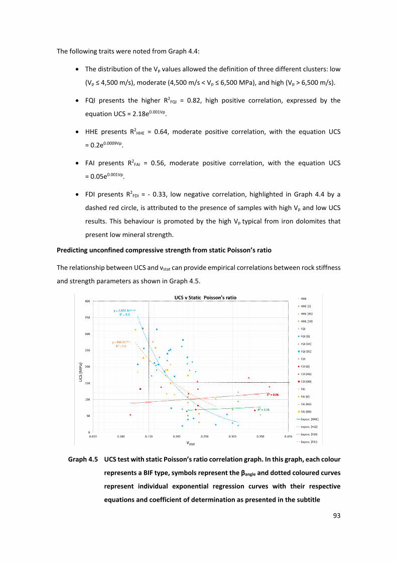
93
The following traits were noted from Graph 4.4:
• The distribution of the Vp values allowed the definition of three different clusters: low
(Vp ≤ 4,500 m/s), moderate (4,500 m/s < Vp ≤ 6,500 MPa), and high (Vp > 6,500 m/s).
• FQI presents the higher R2FQI = 0.82, high positive correlation, expressed by the
equation UCS = 2.18e0.001Vp.
• HHE presents R2HHE = 0.64, moderate positive correlation, with the equation UCS
= 0.2e0.0009Vp.
• FAI presents R2FAI = 0.56, moderate positive correlation, with the equation UCS
= 0.05e0.001Vp.
• FDI presents R2FDI = - 0.33, low negative correlation, highlighted in Graph 4.4 by a
dashed red circle, is attributed to the presence of samples with high Vp and low UCS
results. This behaviour is promoted by the high Vp typical from iron dolomites that
present low mineral strength.
Predicting unconfined compressive strength from static Poisson’s ratio
The relationship between UCS and νstat can provide empirical correlations between rock stiffness
and strength parameters as shown in Graph 4.5.
0-5 Graph 4.5 UCS test with static Poisson’s ratio correlation graph. In this graph, each colour
represents a BIF type, symbols represent the βangle and dotted coloured curves
represent individual exponential regression curves with their respective
equations and coefficient of determination as presented in the subtitle
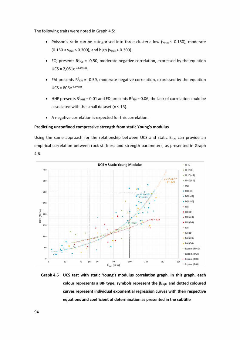
94
The following traits were noted in Graph 4.5:
• Poisson’s ratio can be categorised into three clusters: low (νstat ≤ 0.150), moderate
(0.150 < νstat ≤ 0.300), and high (νstat > 0.300).
• FQI presents R2FQI = -0.50, moderate negative correlation, expressed by the equation
UCS = 2,051e-13.5νstat.
• FAI presents R2FAI = -0.59, moderate negative correlation, expressed by the equation
UCS = 806e-8.6νstat.
• HHE presents R2HHE = 0.01 and FDI presents R2
FDI = 0.06, the lack of correlation could be
associated with the small dataset (n ≤ 13).
• A negative correlation is expected for this correlation.
Predicting unconfined compressive strength from static Young’s modulus
Using the same approach for the relationship between UCS and static Estat can provide an
empirical correlation between rock stiffness and strength parameters, as presented in Graph
4.6.
0-6 Graph 4.6 UCS test with static Young’s modulus correlation graph. In this graph, each
colour represents a BIF type, symbols represent the βangle and dotted coloured
curves represent individual exponential regression curves with their respective
equations and coefficient of determination as presented in the subtitle
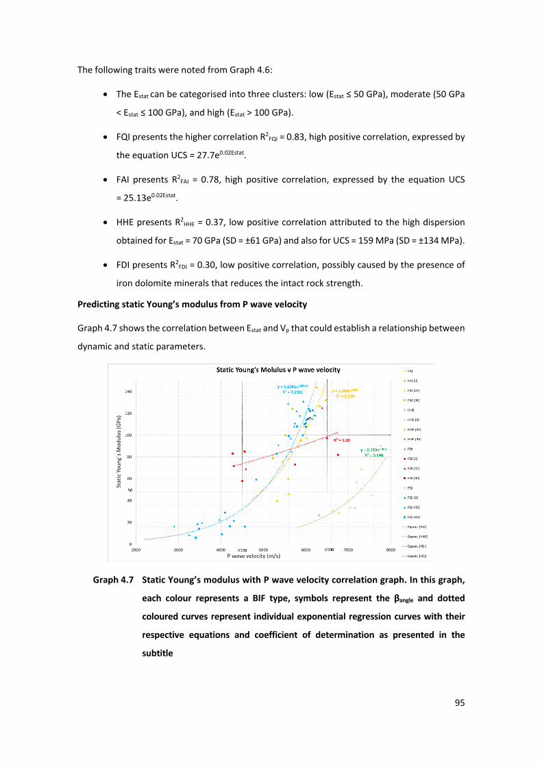
95
The following traits were noted from Graph 4.6:
• The Estat can be categorised into three clusters: low (Estat ≤ 50 GPa), moderate (50 GPa
< Estat ≤ 100 GPa), and high (Estat > 100 GPa).
• FQI presents the higher correlation R2FQI = 0.83, high positive correlation, expressed by
the equation UCS = 27.7e0.02Estat.
• FAI presents R2FAI = 0.78, high positive correlation, expressed by the equation UCS
= 25.13e0.02Estat.
• HHE presents R2HHE = 0.37, low positive correlation attributed to the high dispersion
obtained for Estat = 70 GPa (SD = ±61 GPa) and also for UCS = 159 MPa (SD = ±134 MPa).
• FDI presents R2FDI = 0.30, low positive correlation, possibly caused by the presence of
iron dolomite minerals that reduces the intact rock strength.
Predicting static Young’s modulus from P wave velocity
Graph 4.7 shows the correlation between Estat and Vp that could establish a relationship between
dynamic and static parameters.
0-7 Graph 4.7 Static Young’s modulus with P wave velocity correlation graph. In this graph,
each colour represents a BIF type, symbols represent the βangle and dotted
coloured curves represent individual exponential regression curves with their
respective equations and coefficient of determination as presented in the
subtitle
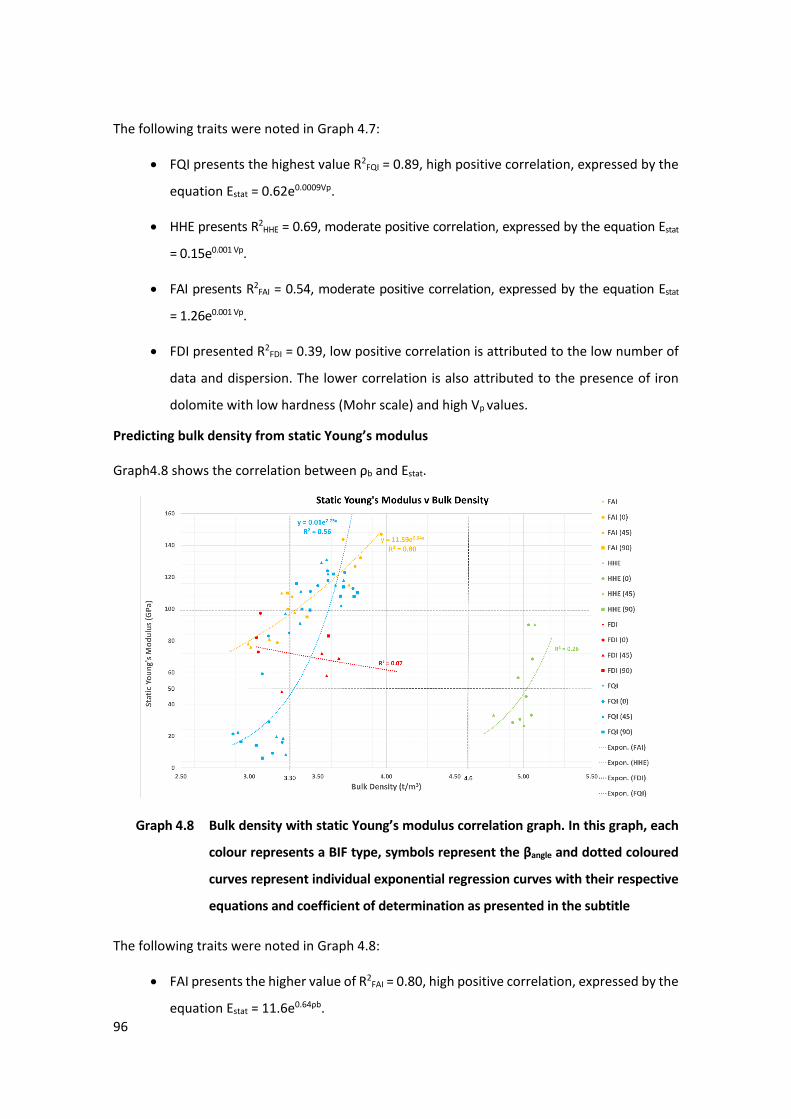
96
The following traits were noted in Graph 4.7:
• FQI presents the highest value R2FQI = 0.89, high positive correlation, expressed by the
equation Estat = 0.62e0.0009Vp.
• HHE presents R2HHE = 0.69, moderate positive correlation, expressed by the equation Estat
= 0.15e0.001 Vp.
• FAI presents R2FAI = 0.54, moderate positive correlation, expressed by the equation Estat
= 1.26e0.001 Vp.
• FDI presented R2FDI = 0.39, low positive correlation is attributed to the low number of
data and dispersion. The lower correlation is also attributed to the presence of iron
dolomite with low hardness (Mohr scale) and high Vp values.
Predicting bulk density from static Young’s modulus
Graph4.8 shows the correlation between ρb and Estat.
0-8 Graph 4.8 Bulk density with static Young’s modulus correlation graph. In this graph, each
colour represents a BIF type, symbols represent the βangle and dotted coloured
curves represent individual exponential regression curves with their respective
equations and coefficient of determination as presented in the subtitle
The following traits were noted in Graph 4.8:
• FAI presents the higher value of R2FAI = 0.80, high positive correlation, expressed by the
equation Estat = 11.6e0.64ρb.
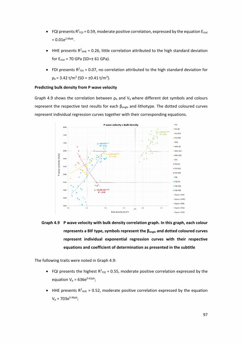
97
• FQI presents R2FQI = 0.59, moderate positive correlation, expressed by the equation Estat
= 0.01e2.66ρb.
• HHE presents R2HHE = 0.26, little correlation attributed to the high standard deviation
for Estat = 70 GPa (SD=± 61 GPa).
• FDI presents R2FDI = 0.07, no correlation attributed to the high standard deviation for
ρb = 3.42 t/m3 (SD = ±0.41 t/m3).
Predicting bulk density from P wave velocity
Graph 4.9 shows the correlation between ρb and Vp where different dot symbols and colours
represent the respective test results for each βangle and lithotype. The dotted coloured curves
represent individual regression curves together with their corresponding equations.
0-9 Graph 4.9 P wave velocity with bulk density correlation graph. In this graph, each colour
represents a BIF type, symbols represent the βangle and dotted coloured curves
represent individual exponential regression curves with their respective
equations and coefficient of determination as presented in the subtitle
The following traits were noted in Graph 4.9:
• FQI presents the highest R2FQI = 0.55, moderate positive correlation expressed by the
equation Vp = 636e0.62ρb;
• HHE presents R2HHE = 0.52, moderate positive correlation expressed by the equation
Vp = 703e0.46ρb;
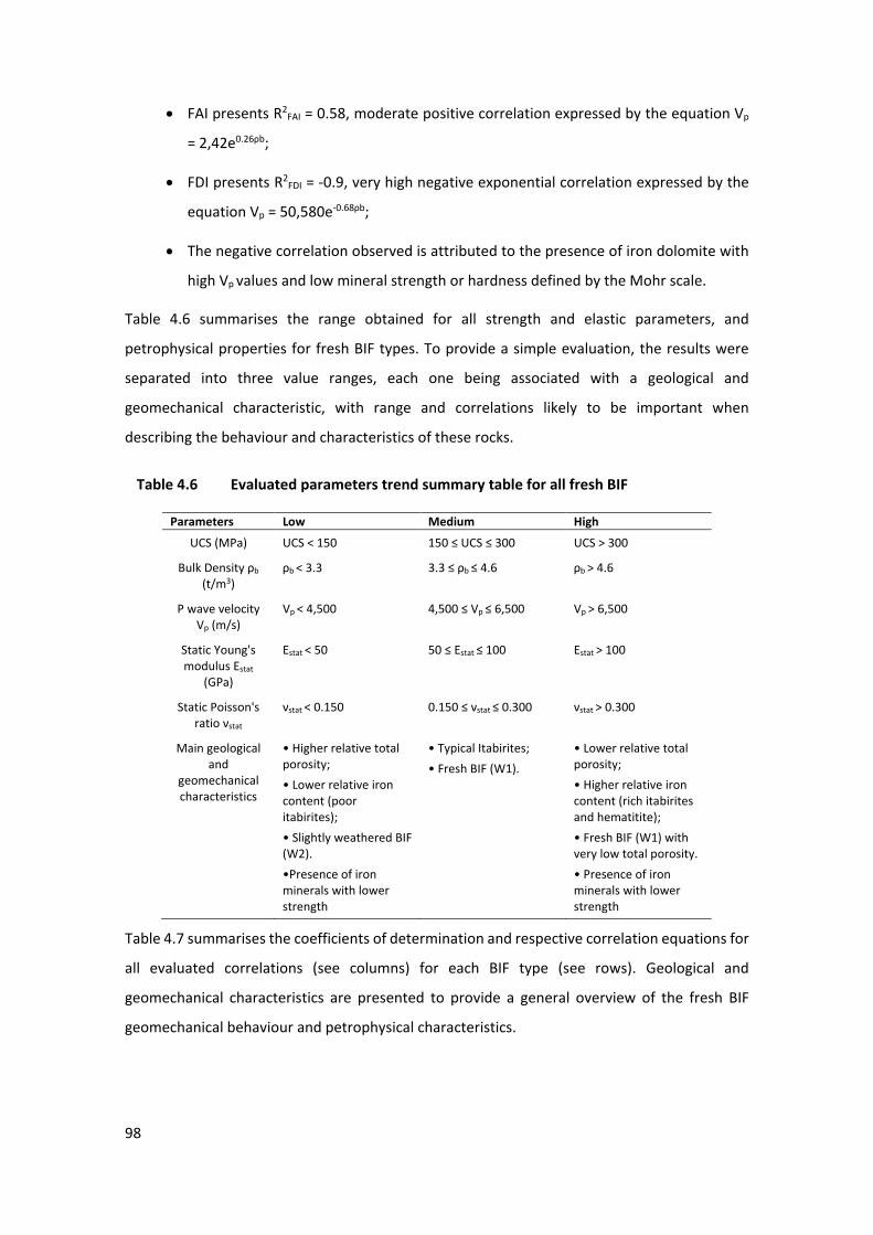
98
• FAI presents R2FAI = 0.58, moderate positive correlation expressed by the equation Vp
= 2,42e0.26ρb;
• FDI presents R2FDI = -0.9, very high negative exponential correlation expressed by the
equation Vp = 50,580e-0.68ρb;
• The negative correlation observed is attributed to the presence of iron dolomite with
high Vp values and low mineral strength or hardness defined by the Mohr scale.
Table 4.6 summarises the range obtained for all strength and elastic parameters, and
petrophysical properties for fresh BIF types. To provide a simple evaluation, the results were
separated into three value ranges, each one being associated with a geological and
geomechanical characteristic, with range and correlations likely to be important when
describing the behaviour and characteristics of these rocks.
6 Table 4.6 Evaluated parameters trend summary table for all fresh BIF
Parameters Low Medium High
UCS (MPa) UCS < 150 150 ≤ UCS ≤ 300 UCS > 300
Bulk Density ρb (t/m3)
ρb < 3.3 3.3 ≤ ρb ≤ 4.6 ρb > 4.6
P wave velocity Vp (m/s)
Vp < 4,500 4,500 ≤ Vp ≤ 6,500 Vp > 6,500
Static Young's modulus Estat
(GPa)
Estat < 50 50 ≤ Estat ≤ 100 Estat > 100
Static Poisson's ratio νstat
νstat < 0.150 0.150 ≤ νstat ≤ 0.300 νstat > 0.300
Main geological and
geomechanical characteristics
• Higher relative total porosity; • Lower relative iron content (poor itabirites); • Slightly weathered BIF (W2). •Presence of iron minerals with lower strength
• Typical Itabirites; • Fresh BIF (W1).
• Lower relative total porosity; • Higher relative iron content (rich itabirites and hematitite); • Fresh BIF (W1) with very low total porosity. • Presence of iron minerals with lower strength
Table 4.7 summarises the coefficients of determination and respective correlation equations for
all evaluated correlations (see columns) for each BIF type (see rows). Geological and
geomechanical characteristics are presented to provide a general overview of the fresh BIF
geomechanical behaviour and petrophysical characteristics.
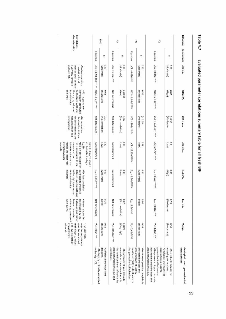
7Table 4.7 Evaluated param
eter correlations summ
ary table for all fresh BIF
Lithotype Correlations
UCS × ρ
b U
CS × Vp
UCS × ν
stat U
CS × Estat
Esta t × V
P E
stat × ρb
VP × ρ
b G
eological and
geomechanical
characteristics
FQI
R2
0.56 (M
oderate) 0.82 (High)
(-)0.50 (M
oderate) 0.3 (Low
) 0.89 (High)
0.59 (M
oderate) 0.55 (M
oderate) •M
ost reliable itabirite forassessing correlations. •G
eological characteristics express typical itabirite geom
echanical behaviour. •The presence of quartz as m
ainnon-iron m
ineral conditions the geom
echanical behaviour.
Equation U
CS = 0.04e2.37ρb
UCS = 2.18e
0.001Vp U
CS = 2,051e-13.5νstat
UC = 27.7e
0.02Estat E
stat = 0.62e
0.0009Vp E
stat = 0.01e2.66ρb
Vp = 636e
0.62ρb
FAI
R2
0.50 (M
oderate) 0.56 (M
oderate) (-) 0.59 (M
oderate) 0.78 (High)
0.54 (M
oderate) 0.80 (High)
0.58 (M
oderate) •Presence of goethite (am
phibole alternated) induces the predom
inance of slightly w
eathered (W2) and influence in
the geomechanical behaviour.
Equation U
CS = 0.03e2.52ρb
UCS = 0.05e
0.001Vp U
CS = 806e-8.6νstat
UCS = 25.13e
0.02Estat E
stat = 1.26e0.001 Vp
Estat 11.6e
0.64ρb V
p = 2,42e0.26ρb
FDI
R2
0.70 (M
oderate) (-) 0.33 (Low
) 0.06 (N
o correlation) 0.30 (Low
) 0.39 (Low
) 0.07 (N
o correlation) (-) 0.9 (Very high)
•The presence of iron dolomite
minerals, as the m
ain mineral in
the nom iron band, influence the
geomechanical behaviour and
correlations.Equation
UCS = 1.18e
1.29ρb N
ot determined
Not determ
ined N
ot determined
Not determ
ined N
ot determined
Vp = 50,580e
-0.68ρb
HHE R
2 0.50 (M
oderate) 0.64 (M
oderate) 0.01 (N
o correlation) 0.37 (Low
) 0.69 (M
oderate) 0.26 (Little)
0.52 (M
oderate) •Different behaviour fromitabirites. •The high 𝜌𝜌
b is directly associatedto the high U
CS. Equation
UCS = 3.23E-06e
3.43 ρb U
CS = 0.2e0.0009Vp
Not determ
ined N
ot determined
Estat = 0.15e
0.001 Vp N
ot determined
VP = 703e
0.46ρb
Correlations characteristics
•Moderate positive
correlation for all types as total porosityis very low
for fresh and hard BIF.
•FDI negative low
correlation attributedto the high V
P SD and the high V
p values ofiron dolom
ite m
inerals.
•No correlation
obtained for HHE and FDI are attributed the high dispersion and sm
all dataset.
•Low HHE correlation is
attributed to the high E
stat SD.•The low
correlation forFDI is associated to the presence of iron dolom
ite minerals that
reduce the intact rock strength (w
eaker m
ineral).
•FDI low correlation
attributed to the small
dataset, low strength and
to the high Vp observed for iron dolom
ite m
inerals.
•No correlation for
FDI induced by the high ρ
b SD and higherferroan dolom
ite m
ineral 𝜌𝜌b com
pared w
ith quartz.
•FDI very high negative correlations m
ust be associated to the high V
p valuesand low
strength of iron dolom
ite m
inerals.
99
100
The high coefficient of determination obtained for some lithotypes between bulk density,
P wave velocity, Young’s modulus and UCS represents a reliable approach able to define intact
rock strength and elastic parameters and describe mechanical characteristics and
geomechanical behaviour of each lithotype. Even for the low coefficient of determination results
obtained, influenced by the high data dispersion observed at some lithotypes, useful knowledge
that can describe the geomechanical behaviour can be observed.
4.6 DISCUSSION
4.6.1 BIF compositional metamorphic banding heterogeneity and strength
anisotropy
Analyses conducted in this research found three main types of petrophysical characteristics of
pervasive fabric responsible for inducing penetrative planes that can result in anisotropy for fresh
BIF:
• Band boundary, fabric contrast (crystal and pore size) at boundary, and contact
between bands of iron and non-iron minerals.
• Mineral orientation, planar or granular minerals oriented along a single or multiple
directions.
• Pore orientation, oriented levels/bands with pore concentration.
These BIF fabric characteristics consist of persistent and repetitive layers or bands that may
define a heterogeneity wherein the anisotropy ratio and index, depending on the BIF type, varies
from isotropic to low anisotropy ratio.
In this context, HHE is a monomineralic (mainly iron minerals) rock, with metamorphic
heterogeneity defined by interlayered bands of low or high total porosity and different shape
and size of iron minerals. For this reason, it is defined macroscopically as homogeneous due to
the difficult to see porous variation without thin section analyses. In contrast, the itabirites, are
heterogeneous rocks with compositional metamorphic banding defined by the repetition of iron
and non-iron mineral bands. From the geomechanical perspective, both can represent a low
transverse anisotropy as defined by the three fabric characteristics, band boundary, pore
orientation, and mineral orientation.
The low visual total porosity observed in BIF the sections, averaging 5% for fresh (W1), reaching
13% for slightly weathered (W2), is an important petrophysical characteristic conditioned by the
rock fabric and weathering. The pore layers or bands represent a pervasive plane and are used
101
as preferential paths for water percolation, inducing leaching and other weathering effects,
responsible for enlarging the pores, and mineral chemical alteration (e.g. oxidation) reducing
parental intact rock strength. Continuous weathering through the rock matrix or mainly by the
pore layers or discontinuities will change in great depths the parental hard and fresh itabirite to
slightly weathered and, depending on the main non-iron mineral, progress the weathering grade
(in shallower depths) to moderately, highly, completely weathered rock, and finally residual soil,
progressively reducing its intact rock strength.
The heterogeneity defined by the non-iron mineral band and the thickness of this band are
important features that controls the bulk density, iron content and, ultimately, the intact rock
strength of itabirite. For hematitite as mineralogically homogenous type, the metamorphic
banding heterogeneity is defined by the alternation of different porous bands normally
associated with the presence of tabular hematites and granoblastic hematite minerals, with a
minor presence of quartz. Additionally, the low strain and low metamorphic grade (green schist)
observed along the western side of the Iron Quadrangle imposed on the relatively simple
mineralogical assemblages of the BIF a fabric with small mineral size and poor orientation that
did not impose strong anisotropy on the intact rock.
Correlating the mineralogical (fabric) behaviour, evidenced by Sections 4.5.1 and 4.5.2, with the
three main fabric domains suggested by Rosière et al. (2001) for western side of the Iron
Quadrangle into:
• Domain 1: Subhedral to euhedral crystals in an overall granoblastic fabric which is the
most common fabric, associated with contact band boundaries and itabirites
heterogeneity, and considered to represent post-tectonic partial recrystallisation;
• Domain 2: Euhedral, composed of locally tabular-shaped and locally very elongated
specularite platelets that induce a preferred mineral orientation;
• Domain 3: Brecciated fabric domain that occurs locally and can be associated with pore
concentration.
Each of these domains will affect BIF intact rock strength, heterogeneity, and anisotropy in
different ways. Domain 1 is considered the main representative and is in accordance with
geological and geomechanical characteristics evaluated. Although domains 2 and 3 are more
restricted in the studied mine sites, they could represent BIF subtypes (breached and sheared)
not evaluated in this chapter.
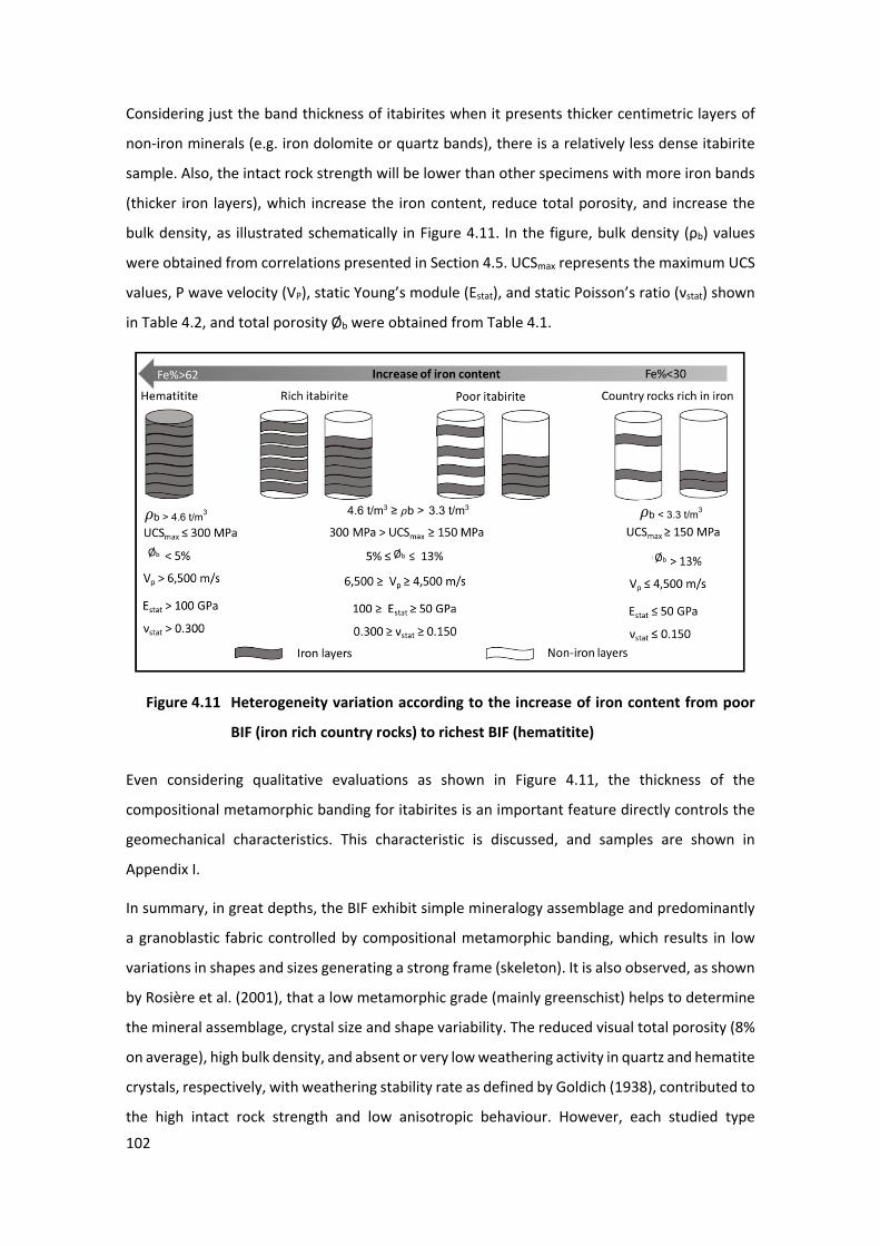
102
Considering just the band thickness of itabirites when it presents thicker centimetric layers of
non-iron minerals (e.g. iron dolomite or quartz bands), there is a relatively less dense itabirite
sample. Also, the intact rock strength will be lower than other specimens with more iron bands
(thicker iron layers), which increase the iron content, reduce total porosity, and increase the
bulk density, as illustrated schematically in Figure 4.11. In the figure, bulk density (ρb) values
were obtained from correlations presented in Section 4.5. UCSmax represents the maximum UCS
values, P wave velocity (VP), static Young’s module (Estat), and static Poisson’s ratio (νstat) shown
in Table 4.2, and total porosity Øb were obtained from Table 4.1.
23 Figure 4.11 Heterogeneity variation according to the increase of iron content from poor
BIF (iron rich country rocks) to richest BIF (hematitite)
Even considering qualitative evaluations as shown in Figure 4.11, the thickness of the
compositional metamorphic banding for itabirites is an important feature directly controls the
geomechanical characteristics. This characteristic is discussed, and samples are shown in
Appendix I.
In summary, in great depths, the BIF exhibit simple mineralogy assemblage and predominantly
a granoblastic fabric controlled by compositional metamorphic banding, which results in low
variations in shapes and sizes generating a strong frame (skeleton). It is also observed, as shown
by Rosière et al. (2001), that a low metamorphic grade (mainly greenschist) helps to determine
the mineral assemblage, crystal size and shape variability. The reduced visual total porosity (8%
on average), high bulk density, and absent or very low weathering activity in quartz and hematite
crystals, respectively, with weathering stability rate as defined by Goldich (1938), contributed to
the high intact rock strength and low anisotropic behaviour. However, each studied type
𝜌𝜌b > 4.6 t/m3 4.6 t/m3 ≥ 𝜌𝜌b > 3.3 t/m3 𝜌𝜌b < 3.3 t/m3
Øb Øb Øb
103
presents individual geomechanical and petrophysical characteristics that represent different
behaviour and results for intact rock strength and deformability.
To assess the existence of this different behaviour, an evaluation of the anisotropy effects
defining the anisotropic ratio using UCS tests and anisotropy index using Vp was presented in
Section 4.3.1. From IVp, all BIF are fairly anisotropic with a slightly higher anisotropy index for FDI
(IVp = 1.3). From the UCS tests (Rc) FDI also presented a low to medium anisotropic ratio (Rc FDI
= 2), while all the other lithotypes were defined as having a low anisotropic ratio. HHE proved to
be the most isotropic in the two techniques used (IVp HHE = 1.1 and Rc HHE = 1).
FDI was defined as the lithotype with higher relative anisotropy (IVp FDI = 1.3 and Rc FDI = 2) this
behaviour is defined by the presence of bands with weaker minerals (iron dolomite), that can
induce strength reduction where these minerals are more concentrated. The bias imposed by
the reduced number of tests at β0° linked to the difficulty to obtain proper samples should also
be considered. The difficulty of preparing proper samples for the different βangle observed for
HHE and FDI is an indirect indication of the lower-strengths of some surfaces that exhibit
elongated minerals such as specularite for HHE and accessory chlorite or talc for FDI.
The intact rock strength of BIF obtained from UCS tests showed a high SD. However, the mean
values are similar with a small range for each type.
4.6.2 Petrophysical, geological and geomechanical properties characterisation and
correlations
The regression curves obtained for the petrophysical and geomechanical property correlations
are summarised and outlined in the following section considering each correlation sets.
UCS and bulk density correlation
As shown in Graph 4.3, all types presented a positive exponential curve with a moderate R2, in
agreement with the references as the increase of intact rock strength increases proportionally
with the bulk density. Clusters with low bulk density and low UCS values are suitable with
itabirite samples with fewer iron bands, and slightly weathered (W2) itabirites and hematitites
due to the slightly high relative total porosity. The R2 increases from FAI and HHE to FQI with
similar values.
FDI shows lower UCS values with mean equal 135 MPa and SD = ±64 MPa (moderate),
representing the lower value from all BIF even presenting low pore content and smaller crystal
size (0.005 mm to 0.87 mm). This lower intact rock strength is attributed to the presence of iron
104
dolomite minerals (siderite and ankerite) which present higher ρb = 2.83 t/m3, when compared
with quartz ρb = 2.65 t/m3, and are considered weaker, in absolute Mohs hardness (also
compared with quartz), inducing a relative lower intact rock strength with no considerable bulk
density reduction. Additionally, the presence of low strength cement (calcite) could be I some
cases, responsible for the lower relative UCS mean value obtained.
The anisotropic ratio obtained for FDI (Rc = 2) is closer to medium anisotropy class and this
variation can be in somehow influence in this relationship.
For FQI, the most common itabirite, with the UCS mean equal to 173 MPa and SD = ±96 MPa
and FAI, with UCS mean equal to 172 MPa and SD = ±89 MPa presented the same UCS value. FAI
and FQI presented similar anisotropic ratios and consequentially strength values, interpreted as
being related to their similar mineral constitution, with quartz as the main non-iron mineral.
The HHE presents the higher bulk density but not the highest UCS mean values, although it
presented the highest individual the UCS test results present the mean equal to 159 MPa and
higher SD = ±134 MPa from all BIF, and a higher maximum UCS test result (UCSmax = 585). The
unexpected slightly lower UCS mean value obtained for the samples with higher ρb, lower total
porosity and absence of non-iron mineral bands is explained by the low number of reliable test
results obtained mainly for β90° and β45° that may bias the mean UCS values for this rock type.
This behaviour can locally be attributed to the influence of thin layers of penetrative, low
strength specularite or tabular hematite at shear surfaces, especially for samples with β90° and
β45°. These micro, highly anisotropic surfaces normally can only be observed in thin sections,
which creates challenges during laboratory selections and evaluations only detected by Vp
measure evaluations.
UCS and P wave velocity correlation
Jamshidi et al. (2018), present a summary table proving important correlation equations
between UCS and Vp obtained from several authors. The positive correlations and equations
obtained here are in accordance with the table proposed by these authors. From Graph 4.4,
HHE, FAI and FQI presented an expected positive exponential correlation curve.
P wave velocity is relatively lower for the itabirite group (FQI to FDI and FAI) with lower iron
content and relative lower bulk density and increase for the hematitite group (HHE) with higher
iron content and relative higher bulk density.
The negative correlation obtained for FDI is explained by the presence of iron dolomite mineral
as the main non-iron band mineral that present a high Vp value (±7,500 m/s), close to the
105
hematite (Vp = ±7,400m/s) and much higher than quartz (Vp = 6,060 m/s) (Fourmaintraux 1976).
Higher Vp velocities for iron dolomite minerals and lower UCS results caused by this mineral
lower hardness, as already explained, can contribute to this atypical correlation. Thus,
mineralogy highly influences the correlation of UCS and Vp for FDI.
UCS and static Poisson’s ratio correlation
Graph 4.5 shows similar behaviour for FAI and FQI, presenting moderate R2 and expected
negative exponential correlation. It is possible to note that as proposed by Li (2014), if quartz
content increases, the Poisson’ ratio decreases as observed for FAI νstat = 0.2 and FQI νstat = 0.19
(quartz-based mineral at non-iron bands) compared with HHE νstat = 0.29 with n quartz bands
and FDI νstat = 0.22 with iron dolomites as the mains non-iron bands.
Little or no correlation were observed for Poisson’s ratio. It is partially attributed to the low
accuracy associated with the measurement of Poisson’s ratio as this parameter is sensitive to
the position of the strain gauges on the samples. For this feature, inaccuracies could be the cause
of the low correlation obtained as the gauges’ positions were not controlled. Additionally, the
deformation which each rock specimen was exhibited (deep and stress dependent) may
influence on this correlation (also not controlled in this research).
UCS and static Young’s modulus correlation
As shown in Graph 4.6, all BIF presented the expected exponential positive correlation curve.
The unexpected low R2 and low mean value obtained for the HHE Estat = 70 GPa (SD = ±61GPa) is
attributed to the presence of pore layers for W2 samples. The low correlation observed for FDI
is attributed to the presence of iron dolomite minerals, which reduces the intact rock strength
due to the relative lower Mohr scale of hardness (value between brackets) presented by calcite
(3) and dolomite (3.5) compared with quartz (7).
Arslan et al. (2008), present a summary table proving important correlation equations between
Estat and UCS obtained from several authors. The correlation and equations obtained here are in
accordance with table proposed by these authors.
Static Young’s modulus and P wave velocity correlation
As observed in Graph 4.7, all lithotypes presented positive exponential curves in accordance
with expected behaviour. The low correlation obtained for FDI is explained by the presence of
iron dolomite as already explained for UCS with Vp correlation.
106
Static Young’s modulus and bulk density correlation
From Graph 4.8, HHE shown higher range and bulk density values, and in contrast, the FDI
presents a small range of bulk density values. The exponential positive correlations obtained for
BIF types are in accordance with expected behaviour and dataset size, as is expected an increase
in Young´s modulus with bulk density increase. The lack of correlation obtained for FDI is
explained by the presence of iron dolomite with higher mineral bulk density compared with
quartz also affecting the correlation; same as verified with other correlations.
P wave velocity and bulk density
Graph 4.9 shows an exponential positive correlations as expected, as Vp increases as ρb increases.
The high negative correlation for FDI is attributed to the high relative Vp of iron dolomite minerals
presented in this type when compared with other itabirites.
The regression curves obtained for the petrophysical and geomechanical property correlations
are summarised and outlined below for each BIF type:
• Hard hematitite
The hard hematitite, as almost monomineralic rock, is constituted mainly of iron oxides and
hydroxides (e.g. hematite and martite) with percentage of pores between 5% and 10%
(Table 4.1). The heterogeneous metamorphic banding is represented by layers with higher total
porosity interlayered with more massive ones, conditioned by the weathering (W2) and mineral
and pores orientation. The Rc and the IVp were isotropic to fairly anisotropic.
Considering anisotropy effects, the UCS varies from 210 MPa to 100 MPa and for the isotropic
mean is 159 MPa. High intact rock strength is mainly defined by the high ρb = 5.02 t/m3, low pore
content and small mineral size (0.001 mm to 0.08 mm). The Vp mean obtained of 7,022 m/s is in
average 30% higher than the other BIF This difference is attributed to the mineral constitute and
higher bulk density of this type.
The most reliable equations, with moderate R2, were obtained for all Vp correlations as presented
in Table 4.7. This pattern is attributed to the higher Vp and ρb obtained for this type compared with
the itabirites group. Estat and νstat proved not to be reliable correlation parameters mainly imposed
by the high SD obtained for UCS results where static elastic parameters are obtained. Since the
anisotropy effects are not important for HHE, the high SD noted could be attributed to the
sample’s intrinsic characteristics mainly by the presence of pores and tabular mineral microlayers
that induces early peak resistance in UCS tests.
107
• Fresh quartzitic itabirite
FQI is the most common BIF lithotype, presenting compositional metamorphic banding
conditioned by concentrated quartz bands interplayed with iron bands representing the typical
itabirite heterogeneity. The degree of anisotropy obtained from different parameters (Rc and
IVp) were low and fair, respectively. The total percentage of pores is less than 11% (Table 4.1).
These higher percentage of pores is concentrated in quartz bands or at the contact between iron
and quartz bands inducing some anisotropy parallel to the compositional metamorphic banding.
These pores are generated by weathering (leaching the quartz and recrystallising different iron
ore oxides and hydroxides), mainly in slightly weathered lithotypes (W2). Increasing percentages
of the pore’s layers potentially (increasing the weathering in shallower depths or fractured
zones) generate preferential weathering paths that can increase the anisotropy and change to
moderately weathered lithotypes to completely weathered ones.
The high intact rock strength is mainly defined by the low pore content and higher percentage
of iron bands defined by the typical itabirite heterogeneity as presented in Figure 4.11. The
variation in intact strength is imposed by chances in the thickness of the compositional bands.
As the iron bands present similar crystal sizes for all itabirites, this characteristic seems to not
influence the UCS results as the mean values are very close (inside the SD).
FQI presented the best correlations from all BIF, with moderate to high coefficients of
correlation providing reliable correlation equations as observed in Table 4.7. The presence of
quartz, with lower bulk density and higher Mohr hardness, compared with iron dolomite band
minerals, may have contributed to this high correlation and high relative UCS mean values.
• Fresh amphibolitic itabirite
With high susceptibility to weathering, FAI is mainly observed in deeper mines. Consequently,
slightly weathered FAI (W2) is widely distributed across studied mines and determining its
geomechanical attributes was considered to be more important than determining those of FAI
(W1). The compositional metamorphic banding is conditioned by mineral concentration of
quartz and goethite (as cement) interplayed with iron bands representing the heterogeneity.
The Rc and Ivp obtained was low and fair, respectively. The mean total percentage of pores is 6%
for typical slightly weathered (W2) specimens as presented in Section 4.5.1.
FAI presents similar high intact rock strength, compared with FQI, mainly defined by the low
pore content and higher percentage of iron bands, as discussed in Section 4.6.1. In addition to
the presence of hematite and goethite cementation observed in this type.
108
This type also presented moderate to high coefficients of determination providing reliable
correlation equations as observed in Table 4.7. The presence of quartz gives to FAI the same
characteristics observed for the FQI. Additionally, the presence of goethite (Vp = 6,950 m/s) may
induce a higher Vp compared with the FQI.
• Fresh dolomitic itabirite
FDI is the type most prone to weathering (leaching the dolomitic bands). The mean total
percentage of pores is 6% as presented in Table 4.1, and the Rc and the Ivp were low to fair,
respectively. However, this represents the higher values obtained from all types (class superior
limit). The different behaviours observed from other itabirites for the FDI can be partially
attributed to the compositional metamorphic banding inducing a slightly higher anisotropy,
which is in turn attributed to the presence of iron dolomite minerals with lower Mohr hardness,
and higher Vp and bulk density when compared with quartz, mainly at non-iron bands.
FDI presents the lowest UCS mean value from all BIF, even presenting relatively lower total
porosity and high ρb similar to FQI and higher from FAI. The same consideration about
heterogeneity addressed for FQI and FAI could be used for FDI. However, the main
characteristics that impose the different behaviour is the presence of iron dolomite minerals in
non-iron bands. These minerals impose negative correlation curves for Vp correlations attributed
to the high Vp and an intact rock strength reduction. Secondarily, the main cementation consists
generally of calcite (low strength cement) that could locally be responsible for lower relative
UCS values and mean obtained contributed to the reduction in intact rock strength and elastic
parameter.
Compared with other itabirites, the FDI presents the most different behaviour, as presented in
Table 4.7. In general, low to no correlations are observed, except for a moderate correlation for
UCS with ρb and very high negative correlation for Vp with ρb.
4.7 CONCLUSION
It is expecting a natural variation obtained experimentally for intact rocky material (even
considering the absence of microcracks), largely due to the randomness of geological and
eventual experimental errors, which, without a doubt, should manifest themselves even in
samples of the same lithology tested in a common anisotropy direction. However, the results
showed a variation beyond what was initially expected, even with all the criteria adopted to
eliminate outliers, which must be linked to the natural heterogeneity of the tested rocks, a fact
that must be considered in the analyses involving these materials.
109
As experienced, geological features induce large dispersions of the results, since they may have
different variations in fabric, affected by rock heterogeneity and early influence of weathering,
inducing small but not irrelevant anisotropy effects, and variations in the petrophysical
properties of the samples (e.g. ρb and Øb). Even so, using several methodologies (samples
separation and statistical methods) it was possible to verify reliable trends of a correlation
mainly for HHE, FAI and FQI.
A field survey provided geological and geotechnical characterisation applied to group and
remove non-suitable laboratory test results from the dataset reducing bias and data variance.
This approach emphasised the role of identifying the geological characteristics that were crucial
to define a proper sample grouping to separate and better represent the three different types
of fresh itabirites. After this initial step, based on laboratory tests, it was possible to evaluate
the intact rock strength and its static deformability parameters. Thin sections added important
information to explain each rock fabric behaviour and correlation with results from laboratory
tests.
Additionally, even with several attempts to reduce data dispersion, the FDI some parameters
showed high SD. This may represent a natural range expected for each property and also be
attributed to dispersions caused by intrinsic geological features, or by the slightly higher
anisotropic effects observed for FDI.
Three main petrophysical characteristics in the rock fabric were found to be responsible for
inducing penetrative planes that could result in low anisotropies for fresh BIF:
• Heterogeneity – the contact between iron and non-iron minerals bands, which define
the itabirites compositional metamorphic banding.
• Mineral orientation – planar or granular minerals oriented along a single or multiple
directions which also define the metamorphic banding.
• Pores concentration and orientation – oriented porous layers defining the hematitite
metamorphic banding.
Due to the high SD observed for UCS results, the importance of transverse anisotropy for intact rock
strength in each type must be considered with some reservation. Anisotropy effects due to the
compositional banding (heterogeneity) for fresh itabirites (FAI and FQI) and pore concentration
banding for hard hematitites cause minor effects on the intact rock strength. However, as FDI
presents low anisotropy but with a range close to the medium anisotropy class and different
correlations from those obtained for other itabirites, the anisotropy must be considered.
110
From the research finding, it was possible to group fresh BIF into two similar behaviour types:
• Hematitite group – mostly for hard hematitite (HHE), is defined as the isotropic type,
mineralogically homogeneous but with metamorphic banding heterogeneity is defined
by different percentages of pore bands. This group is characterised as the highest bulk
density, P wave velocity, and high UCS values. For this type, the empirical correlations
between UCS with ρb and P wave velocity, and between Vp with ρb and Estat showed
reliable correlation equations.
• Itabirite group – includes all the three fresh itabirites (FAI, FQI and FDI) that showed
several similarities in their definition and characterisation. However, some
particularities can be used for individualisation. A characteristic of this group is the
lower relative ρb, and UCS values and elastic parameters dispersion deeply associated
with the itabirite heterogeneity (defined by the mineral composition and band
thickness), and the low anisotropic behaviour.
This itabirite group was divided into two subgroups defined by the main mineral present in the
non-iron band:
• Quartz based itabirites (FAI and FQI) – low anisotropic material present higher UCS
values and ρb presented reliable equations for all evaluated correlations.
• Iron dolomite based itabirite (FDI) – Presents Ivp and Rc slightly closer to the medium
anisotropy class. This subgroup showed low ρb and UCS results, and few reliable
equations due to the obtained correlations generally in opposition to the other itabirites.
This behaviour is attributed to the intrinsic characteristics of the iron dolomite minerals
with present higher relative Vp, and lower Mohr hardness scale compared with quartz
inducing a lower intact rock strength.
UCS test results proved to be adequate for distinguishing the intact strength variance, from
homogeneous and almost isotropic hard hematitite to heterogeneous and low anisotropic fresh
itabirites, and effective in distinguishing the changes between different compositional itabirites.
Due to the general low porosity of fresh BIF (Øb<5%), the bulk density is directly correlated to
the iron content and an increase in the intact rock strength is proportional with the increase of
iron bands in the specimen. This proportionality was not deeply evaluated in this research.
However, it is suggested that the correlation between UCS and ρb could be used to infer the UCS
values as presented in Appendix I.
111
Moderate (in general) to high and very high coefficients of determination and adjusted regression
curves provided reliable equations for FAI and FQI and made it possible to claim that petrophysical
and elastic properties of the intact rock obtained from dynamic tests, were useful for supporting
the correlations and determining the intact rock strength and deformability parameters of these
types. By contrast, FDI and HHE presented low correlation variations imposed by the intrinsic
characteristics that should be considered when evaluating these types of correlations. These lower
correlations could be related to the Vp being more sensitive to elastic modulus than bulk density
as proposed by Marques et al. (2010). Even the low coefficient of determination observed for some
lithotypes represents useful data for describing geomechanical behaviour.
Findings from the experimental works and basic statistical analyses showed that this study
provided a reliable method of predicting the BIF typology, UCS and elastic parameters and
indirectly establish petrophysical characteristics for ρb, Øb, and Vp.
The field geological and geomechanical investigations, thin sections and laboratory tests
undertaken during the research programme enabled the assessment of the effect of physical
heterogeneity and anisotropy on the geomechanical properties, intact rock strength and elastic
parameters of the BIF and allowed for the development of procedures and equations that will
optimise slope stability evaluations, promote a better understanding of potential slope failure
mechanisms and reduce the risk of slope failure – gains that will help Vale and other iron ore
mines improve the operational productivity and safety of their mines.

112
113
CHAPTER 5. PETROPHYSICAL CHARACTERISTICS AND ELASTIC DYNAMIC
PROPERTIES OF FRESH TO MODERATELY WEATHERED BRAZILIAN BANDED
IRON FORMATIONS
This chapter presents the second unpublished manuscript.
ABSTRACT
Over recent decades, a worldwide iron ore boom has fuelled a rapid increase in pit depths of
Brazilian iron ore mines, especially at mines located in the Iron Quadrangle. This has been due to
environmental restrictions and urban pressure on the lateral expansion of mines. For this reason,
the weak material has been mined and the presence of fresh banded iron formations on final
slopes has become more plentiful, and failure mechanisms and slope instability controlled by
discontinuities and hard rock behaviour have become more common. To support this new
challenge, in mines where instabilities were mainly composed of hard rock materials, rock
mechanics approaches became necessary. These approaches must be based on reliable
geological, structural and geotechnical investigations supported by laboratory test databases.
Strength and elastic properties of rock materials are important parameters used for limit
equilibrium and stress–strain analyses in slope stability and design. It is possible to obtain these
parameters by fast, indirect, and non-destructive dynamic tests supported by empirical
correlation methods, rather than destructive tests that require high-quality cores and
techniques.
An extra challenge to determine these parameters and correlations is posed by the anisotropy
and heterogeneity observed in banded iron formations BIF that can define different parameters
for different anisotropy directions.
Based on geological and geotechnical field investigation, thin sections evaluation, P and S wave
velocity propagation, total porosity and bulk density tests, from a special apparatus (poro
permeameter – AutoLab-500®) this study proposes empirical correlations between dynamic
elastic parameters (Young´s modulus and Poisson’s ratio) and petrophysical parameters (bulk
density and total porosity), for fresh and moderately BIF.
For these proposals, five lithologies have been tested in three different anisotropy planes, defined
by the compositional metamorphic banding (heterogeneity), to provide the anisotropic index and
identify elastic modules and petrophysical correlations.
114
Results show that mineral composition, rock fabric, total porosity and bulk density have the
greatest influence on anisotropy index and elastic (dynamic) properties. The evaluated
assemblage of BIF types was grouped by similar behaviour:
• Fresh to slightly weathered itabirites group, with typical high range for wave velocity,
Young´s modulus values and bulk density, and total porosity.
• Fresh hematitite group, with higher wave velocity, Young´s modulus values and bulk
density, and very lower total porosity.
• Moderately weathered itabirites group, with lower wave velocities, Young´s modulus
values and bulk density, and higher total porosity.
The anisotropy index was isotropic for dolomitic itabirite, and fairly anisotropic for hard
hematitite, fresh quartzitic and amphibolitic itabirites, defined by the mineral composition, rock
fabric, and total porosity. For moderately weathered quartzitic and goethitic itabirites the
anisotropy index is higher (moderately anisotropy index) due to the higher total porosity and
lower bulk density as the weathering process increases. However, this behaviour could be
affected by iron oxides or hydroxides remobilisation and cementation, depending on the
weathering level.
The use of correlations graphs to evaluate dynamic elastic characteristics, petrophysical
properties and predict correlation equations to define geomechanical parameters has proved to
be a reliable methodology to estimate the lithotype that is directly associated with these
geomechanical characteristics. Additionally, the weathering horizons (degree) and
heterogeneity were defined as an important feature that controls anisotropy, bulk density,
elastic parameters and, ultimately, the intact rock strength of the BIF.
5.1 INTRODUCTION
Over recent decades, a booming worldwide iron ore market has put pressure on local and global
iron ore mines to increase their production by - innovative technologies, opening new mines,
and expanding existing mines, not only in width but mainly in depth, to meet this high demand.
For this reason, after decades of mining soil-like and weak rock from the deep weathered
profiles and evaluating slope stability analyses based on soil mechanics principles, Brazilian iron
ore mines are now experiencing new challenges related to deep open pits, where fresh and hard
rock predominate.
115
These iron ore mines are developed in BIF deposits, originally described by Dorr (1969) as a high-
grade ore, called hematite (most recently denominated hematitite) and a low-grade ore, called
itabirite. The original mineralogical composition of non-iron bands, consisting of dolomitic,
amphibolitic and quartzitic layers are used to differentiate itabirite types. In addition, those
lithotypes are the hardest (fresh) BIF seen in Iron Quadrangle iron ore mines.
These four fresh and hard BIF lithotypes, and two subtypes derived from moderately weathered
alteration, were tested in three different anisotropy planes, defined by the metamorphic
banding (heterogeneity plane), to prove the anisotropic index, identify elastic rock properties,
and establish petrophysical (physical rock properties) correlations.
These BIF are easily recognised in mines and the proper assessment of intact rock strength and
elastic parameters is essential for implementing robust geotechnical models for engineering
purposes and slope stability analyses. In addition, for two moderately weathered itabirites
(quartzitic and goethitic) the intact rock strength reduction imposed by weathering reduces the
original fresh and hard behaviour becoming a mixture of hard and weak material. Characterising
such behaviour will be essential to understand this ambiguous comportment, define the
boundary between soil and rock materials, and apply the proper geomechanical approach for
each case.
For decades, in Brazilian iron ore mines the slope stability analysis and design reviews were
based on limit equilibrium techniques supported by the soil mechanics approach. For deep and
hard rock mines, this approach can be insufficient, and to address this problem rock mechanics
must be considered and more robust computational approaches are necessary where the elastic
parameters (Young's and Poisson’s ratio) are important inputs for these applications.
The acquisition of such data using classical rock tests can be time-consuming, costly and,
sometimes, not feasible due to the difficulty of obtaining reliable representative samples from
the field or due to the difficulty of preparing proper samples for laboratory tests or even to the
rock test apparatus setup difficulties (e.g. position of gauges and anisotropy). Otherwise,
dynamic testing is a reliable, low-cost, fast, and non-destructive analysis used to provide
effective and reliable correlations capable of replacing traditional static mechanical tests, such
as uniaxial compressive strength (UCS). Nevertheless, the calibration and analysis of dynamic
effects also requires a minimum number of static laboratory tests.
Based on geological and geotechnical field investigation, thin sections evaluation, P and S wave
velocities propagation, total porosity and bulk density tests undertaken in a high pressure pore
permeameter (AutoLab-500®) this study proposes empirical correlations curves and equations
116
capable of defining dynamic elastic parameters (Young´s modulus and Poisson’s ratio) and
petrophysical parameters (bulk density and total porosity), for fresh and moderately weathered
Brazilian BIF.
5.2 OBJECTIVES AND APPROACHES
Many studies have been undertaken to determine and establish relationships among
petrophysical and dynamic properties for several rock types. From these, only a few studies have
been focused on BIF. This chapter presents petrophysical and dynamic property results for
several Brazilian BIF, with the aim of establishing correlations through the regression technique
(linear or non-linear). The degree of association between these variables was measured by the
coefficient of determination in an attempt to derive reliable empirical approaches for a better
comprehension of geomechanical and anisotropy behaviour, and to provide basic statistical
correlations.
The main aim of this chapter is to evaluate elastic intact rock and petrophysical properties based
on laboratory tests and geological/geotechnical field evaluations and establish correlations for
fresh to moderately weathered BIF.
The main statements to be evaluated in the study are summarised below:
• Evaluate and compare from different types of BIF the dynamic elastic parameters and
geological and geomechanical features.
• Evaluate the influence of the anisotropy and heterogeneity, defined by the
metamorphic banding, in the dynamic elastic parameters.
• Establish a correlation between petrophysical, geological (macro and micro properties)
and geomechanical characteristics with elastic dynamic parameters.
To address this work, this PhD research project was undertaken by the lead author at the
Australian Centre for Geomechanics, School of Civil, Environmental and Mining Engineering, The
University of Western Australia, sponsored by Vale S.A. The main aim of the thesis was to
investigate the complete weathering profile characteristics, from fresh and hard to weak
residual soil of BIF from several Brazilian iron ore mine sites.
This chapter is focused on dynamic intact rock properties, trying to understand the effect of
petrophysical heterogeneity and anisotropy, and attempts to provide practical estimates and
realistic correlations that could replace the lack of intact rock strength parameters. In order to
fully represent the geological influence, these correlations consider dynamic intact rock
117
properties such as mineralogical composition, fabric, bulk density, iron content and other
features.
The heterogeneity and anisotropy defined by the BIF compositional metamorphic banding have
been studied and discussed to address the limitations and drawbacks imposed by compositional
metamorphic banding in the BIF. Because of the research emphasis on intact rock properties,
anisotropy caused by discontinuities (e.g. fractures and joints) was not evaluated.
The emphasis of this research is focussed on the following unweathered BIF lithotypes:
hematitite (HHE), fresh dolomitic (FDI), amphibolitic (FAI) and quartzitic (FQI) itabirites, also
includes moderately weathered materials defined as partially weathered goethitic (PWGI) and
quartzitic (PWQI) itabirites. These rock types were characterised based on four key laboratory
tests: bulk density (ρb), petrographic thin sections, total porosity (poro-permeameter test), and
VP and VS wave velocity determination. The tests results have been summarised and reviewed
to assess the associations that are further identified and explored between these parameters
and elastic dynamic parameters.
5.3 GEOLOGICAL AND GEOTECHNICAL SETTINGS
5.3.1 Regional geological settings
The studied mines are located at the western limb of the Iron Quadrangle in the Moeda Syncline
and Curral Homocline ranges located in the centre of the state of Minas Gerais, Brazil, and part
of Vale’s South Ferrous Division. The seven evaluated mines are Águas Claras (MAC), Capão
Xavier (CPX), Tamanduá (TAM), Capitão do Mato (CMT), Galinheiro (GAL), Pico (PIC), and
Jangada (JGD), with locations shown in Figure 5.1.
The Iron Quadrangle forms a mega structure, which is delineated by a roughly quadrangular
arrangement, with ridges of Paleoproterozoic BIF from the Minas Supergroup, as proposed by
Dorr (1969). These iron deposits are classified as Superior Type, according to Gross (1980) and
are composed of 1,000 m of metamorphic iron ore rocks belonging to the Itabira Group, Cauê
Formation. The Minas Supergroup includes, from bottom to top, Caraça, Itabira, Piracicaba, and
Sabará groups, as a sequence of psammitic pelitic rocks, superimposed by the Itacolomi Group.
Below that sequence are the Archean greenstone terrains of the Rio das Velhas Supergroup and
domes of Archean and Proterozoic crystalline rocks (Machado & Carneiro 1992; Machado et al.
1989 and Noce 1995).
118
According to Chemale Jr et al. (1994), the regional structure is the result of two main
deformational superimposed events. The first produced the nucleation of regional synclines in
the uplift of the gneissic domes during the Trans–Amazonian Orogenesis (2.1–2 Gyr), and the
second is related to an east–west verging thrust fault belt of Pan African/Brazilian age
(0.8–0.6 Gyr) described by Marshak & Alkmim (1989). This last event deformed the earlier
structures and was responsible for the east–west deformational gradient.
Hertz (1978) described an eastward increase in the metamorphic grade and followed the
deformational gradient from greenschist to the lower amphibolite’s facies.
The Cauê Formation (Itabira Group) represents the main host of BIF and defines a marine
chemical sequence of 350 m thick, dated 2.4 ± 0.19 Gyr (Babinski et al. 1995).
The Iron Quadrangle BIF are Paleoproterozoic, metamorphic and heterogeneous banded rocks,
presenting a millimetre to centimetre rhythmic alternation banding of iron minerals (hematite,
martite and magnetite), and non-iron minerals (quartz, dolomite, and amphibolite). Two main
lithologies were defined by Dorr (1969) for this type of iron deposit: hematite, recently
redescribed by Selmi et al. (2009) as hematitite – the high-grade ore (Fe ≥ 62%), and the
low-grade ore, the itabirite (30% < Fe < 62%), with three compositional types or lithotypes,
according to the presence and relative abundance of gangue minerals: quartzitic, dolomitic and
amphibolitic (all defined as proto-ore). Tectonic, metamorphic, and weathering processes have
changed it in different ways, resulting in multiple sets of iron ore lithotypes.
Banding is the most typical characteristic defined by strong heterogeneity. This variation could
be controlled by the original sedimentary bedding, tectonic setting, metamorphic grade,
hydrothermal, or supergene processes. However, the superposition of these processes causes
partial or total mineralogical and textural changes.
The origin of itabirites and associated high-grade hematitite orebodies remains controversial,
and several studies have been produced on this topic, as largely discussed in Spier et al. (2003).
For the genesis of friable orebodies, some authors agree with a supergene process and residual
itabirite enrichment from the leaching of gangue mineral by surface waters. For such orebodies,
the 40Ar/39Ar dating of manganese minerals in Vale mines suggests that weathering processes
and the mineralisation period occurred between 61.5 ± 1.2 Myr to 14.2 ± 0.8 Myr, reaching the
peak process in 51 Myr (Spier 2005 and Spier et al. 2006). This dating indicates a tertiary
mineralisation, and after this period the further weathering may not have substantially affected
the weathering profile.
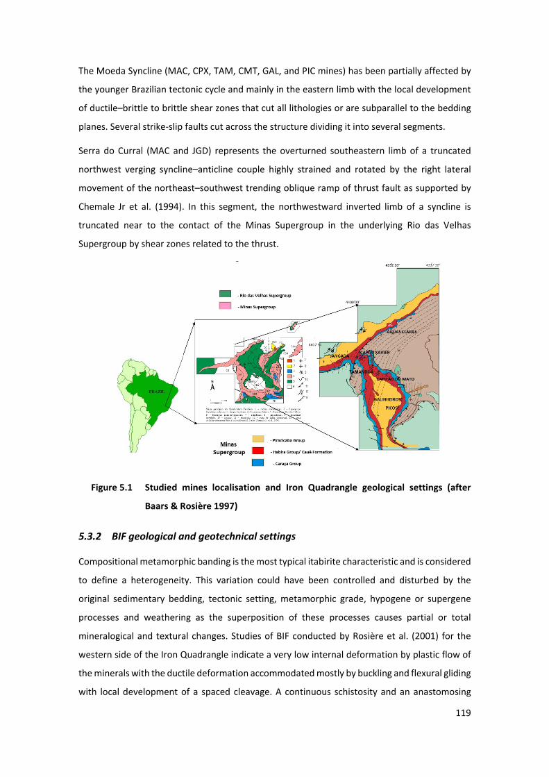
119
The Moeda Syncline (MAC, CPX, TAM, CMT, GAL, and PIC mines) has been partially affected by
the younger Brazilian tectonic cycle and mainly in the eastern limb with the local development
of ductile–brittle to brittle shear zones that cut all lithologies or are subparallel to the bedding
planes. Several strike-slip faults cut across the structure dividing it into several segments.
Serra do Curral (MAC and JGD) represents the overturned southeastern limb of a truncated
northwest verging syncline–anticline couple highly strained and rotated by the right lateral
movement of the northeast–southwest trending oblique ramp of thrust fault as supported by
Chemale Jr et al. (1994). In this segment, the northwestward inverted limb of a syncline is
truncated near to the contact of the Minas Supergroup in the underlying Rio das Velhas
Supergroup by shear zones related to the thrust.
24 Figure 5.1 Studied mines localisation and Iron Quadrangle geological settings (after
Baars & Rosière 1997)
5.3.2 BIF geological and geotechnical settings
Compositional metamorphic banding is the most typical itabirite characteristic and is considered
to define a heterogeneity. This variation could have been controlled and disturbed by the
original sedimentary bedding, tectonic setting, metamorphic grade, hypogene or supergene
processes and weathering as the superposition of these processes causes partial or total
mineralogical and textural changes. Studies of BIF conducted by Rosière et al. (2001) for the
western side of the Iron Quadrangle indicate a very low internal deformation by plastic flow of
the minerals with the ductile deformation accommodated mostly by buckling and flexural gliding
with local development of a spaced cleavage. A continuous schistosity and an anastomosing
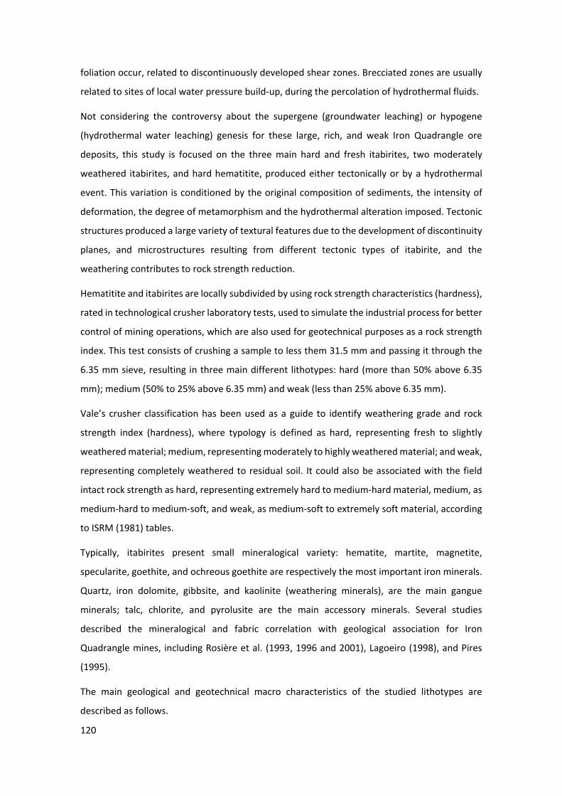
120
foliation occur, related to discontinuously developed shear zones. Brecciated zones are usually
related to sites of local water pressure build-up, during the percolation of hydrothermal fluids.
Not considering the controversy about the supergene (groundwater leaching) or hypogene
(hydrothermal water leaching) genesis for these large, rich, and weak Iron Quadrangle ore
deposits, this study is focused on the three main hard and fresh itabirites, two moderately
weathered itabirites, and hard hematitite, produced either tectonically or by a hydrothermal
event. This variation is conditioned by the original composition of sediments, the intensity of
deformation, the degree of metamorphism and the hydrothermal alteration imposed. Tectonic
structures produced a large variety of textural features due to the development of discontinuity
planes, and microstructures resulting from different tectonic types of itabirite, and the
weathering contributes to rock strength reduction.
Hematitite and itabirites are locally subdivided by using rock strength characteristics (hardness),
rated in technological crusher laboratory tests, used to simulate the industrial process for better
control of mining operations, which are also used for geotechnical purposes as a rock strength
index. This test consists of crushing a sample to less them 31.5 mm and passing it through the
6.35 mm sieve, resulting in three main different lithotypes: hard (more than 50% above 6.35
mm); medium (50% to 25% above 6.35 mm) and weak (less than 25% above 6.35 mm).
Vale’s crusher classification has been used as a guide to identify weathering grade and rock
strength index (hardness), where typology is defined as hard, representing fresh to slightly
weathered material; medium, representing moderately to highly weathered material; and weak,
representing completely weathered to residual soil. It could also be associated with the field
intact rock strength as hard, representing extremely hard to medium-hard material, medium, as
medium-hard to medium-soft, and weak, as medium-soft to extremely soft material, according
to ISRM (1981) tables.
Typically, itabirites present small mineralogical variety: hematite, martite, magnetite,
specularite, goethite, and ochreous goethite are respectively the most important iron minerals.
Quartz, iron dolomite, gibbsite, and kaolinite (weathering minerals), are the main gangue
minerals; talc, chlorite, and pyrolusite are the main accessory minerals. Several studies
described the mineralogical and fabric correlation with geological association for Iron
Quadrangle mines, including Rosière et al. (1993, 1996 and 2001), Lagoeiro (1998), and Pires
(1995).
The main geological and geotechnical macro characteristics of the studied lithotypes are
described as follows.
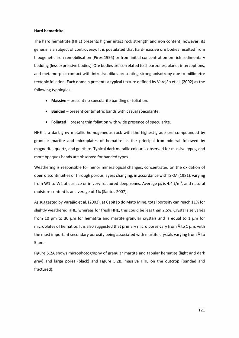
121
Hard hematitite
The hard hematitite (HHE) presents higher intact rock strength and iron content; however, its
genesis is a subject of controversy. It is postulated that hard-massive ore bodies resulted from
hipogenetic iron remobilisation (Pires 1995) or from initial concentration on rich sedimentary
bedding (less expressive bodies). Ore bodies are correlated to shear zones, planes interceptions,
and metamorphic contact with intrusive dikes presenting strong anisotropy due to millimetre
tectonic foliation. Each domain presents a typical texture defined by Varajão et al. (2002) as the
following typologies:
• Massive – present no specularite banding or foliation.
• Banded – present centimetric bands with casual specularite.
• Foliated – present thin foliation with wide presence of specularite.
HHE is a dark grey metallic homogeneous rock with the highest-grade ore compounded by
granular martite and microplates of hematite as the principal iron mineral followed by
magnetite, quartz, and goethite. Typical dark metallic colour is observed for massive types, and
more opaques bands are observed for banded types.
Weathering is responsible for minor mineralogical changes, concentrated on the oxidation of
open discontinuities or through porous layers changing, in accordance with ISRM (1981), varying
from W1 to W2 at surface or in very fractured deep zones. Average ρb is 4.4 t/m3, and natural
moisture content is an average of 1% (Santos 2007).
As suggested by Varajão et al. (2002), at Capitão do Mato Mine, total porosity can reach 11% for
slightly weathered HHE, whereas for fresh HHE, this could be less than 2.5%. Crystal size varies
from 10 μm to 30 μm for hematite and martite granular crystals and is equal to 1 μm for
microplates of hematite. It is also suggested that primary micro pores vary from Å to 1 μm, with
the most important secondary porosity being associated with martite crystals varying from Å to
5 μm.
Figure 5.2A shows microphotography of granular martite and tabular hematite (light and dark
grey) and large pores (black) and Figure 5.2B, massive HHE on the outcrop (banded and
fractured).
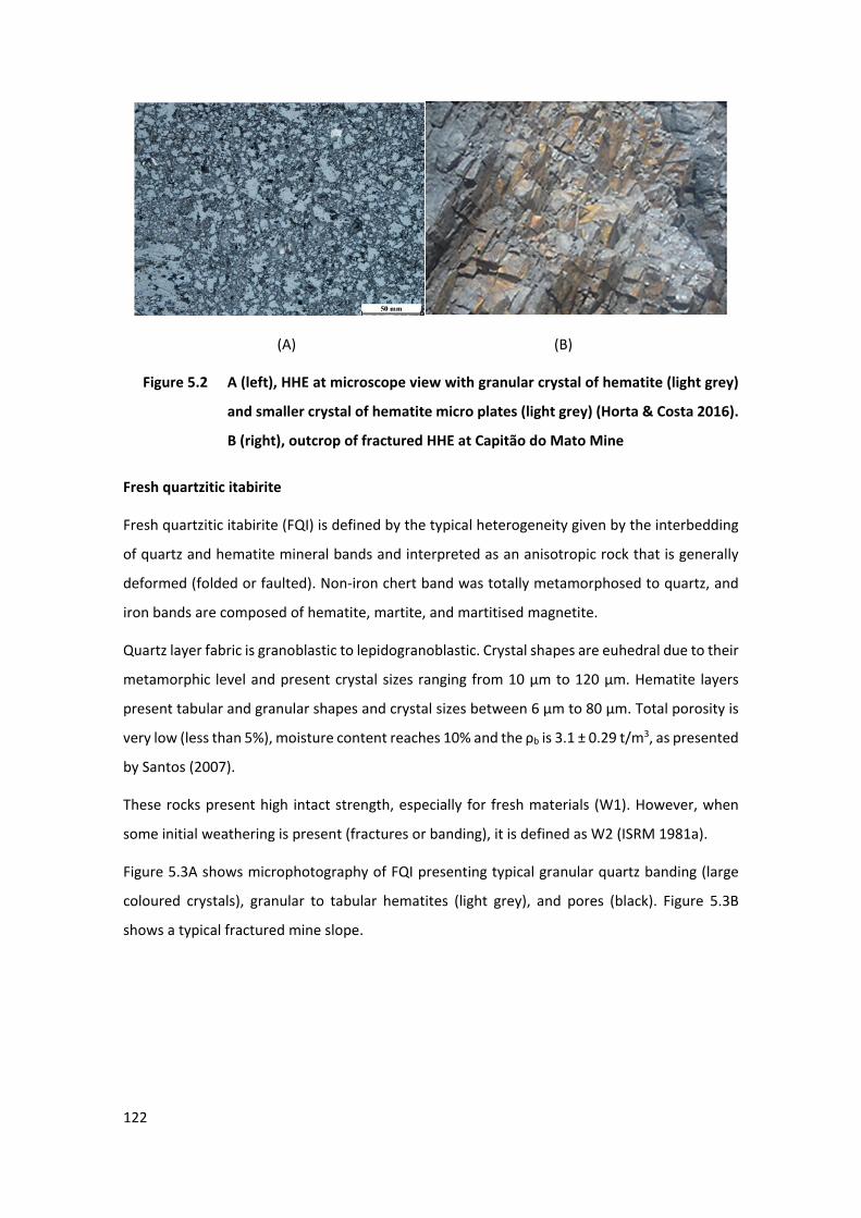
122
(A) (B)
25 Figure 5.2 A (left), HHE at microscope view with granular crystal of hematite (light grey)
and smaller crystal of hematite micro plates (light grey) (Horta & Costa 2016).
B (right), outcrop of fractured HHE at Capitão do Mato Mine
Fresh quartzitic itabirite
Fresh quartzitic itabirite (FQI) is defined by the typical heterogeneity given by the interbedding
of quartz and hematite mineral bands and interpreted as an anisotropic rock that is generally
deformed (folded or faulted). Non-iron chert band was totally metamorphosed to quartz, and
iron bands are composed of hematite, martite, and martitised magnetite.
Quartz layer fabric is granoblastic to lepidogranoblastic. Crystal shapes are euhedral due to their
metamorphic level and present crystal sizes ranging from 10 µm to 120 µm. Hematite layers
present tabular and granular shapes and crystal sizes between 6 µm to 80 µm. Total porosity is
very low (less than 5%), moisture content reaches 10% and the ρb is 3.1 ± 0.29 t/m3, as presented
by Santos (2007).
These rocks present high intact strength, especially for fresh materials (W1). However, when
some initial weathering is present (fractures or banding), it is defined as W2 (ISRM 1981a).
Figure 5.3A shows microphotography of FQI presenting typical granular quartz banding (large
coloured crystals), granular to tabular hematites (light grey), and pores (black). Figure 5.3B
shows a typical fractured mine slope.
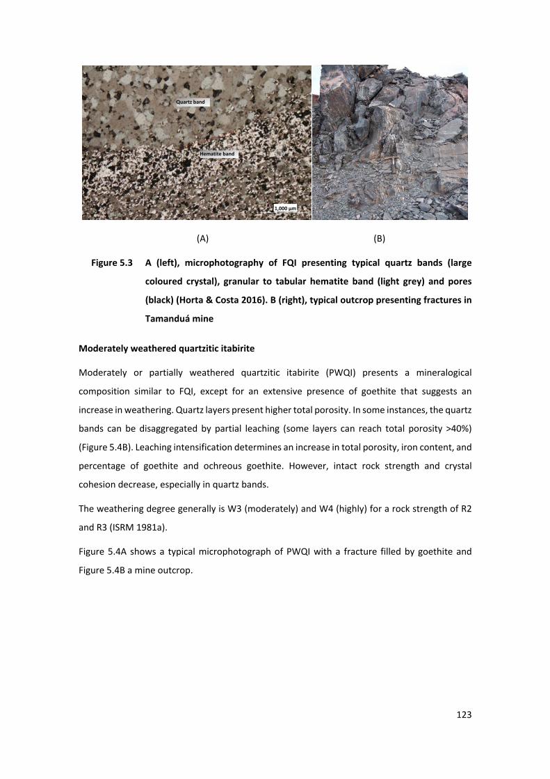
123
(A) (B)
26 Figure 5.3 A (left), microphotography of FQI presenting typical quartz bands (large
coloured crystal), granular to tabular hematite band (light grey) and pores
(black) (Horta & Costa 2016). B (right), typical outcrop presenting fractures in
Tamanduá mine
Moderately weathered quartzitic itabirite
Moderately or partially weathered quartzitic itabirite (PWQI) presents a mineralogical
composition similar to FQI, except for an extensive presence of goethite that suggests an
increase in weathering. Quartz layers present higher total porosity. In some instances, the quartz
bands can be disaggregated by partial leaching (some layers can reach total porosity >40%)
(Figure 5.4B). Leaching intensification determines an increase in total porosity, iron content, and
percentage of goethite and ochreous goethite. However, intact rock strength and crystal
cohesion decrease, especially in quartz bands.
The weathering degree generally is W3 (moderately) and W4 (highly) for a rock strength of R2
and R3 (ISRM 1981a).
Figure 5.4A shows a typical microphotograph of PWQI with a fracture filled by goethite and
Figure 5.4B a mine outcrop.
Hematite band
Quartz band
1,000 μm
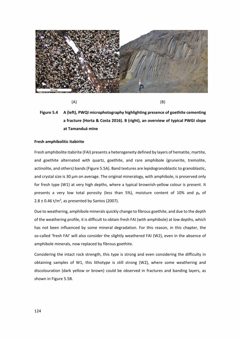
124
(A) (B)
27 Figure 5.4 A (left), PWQI microphotography highlighting presence of goethite cementing
a fracture (Horta & Costa 2016). B (right), an overview of typical PWGI slope
at Tamanduá mine
Fresh amphibolitic itabirite
Fresh amphibolite itabirite (FAI) presents a heterogeneity defined by layers of hematite, martite,
and goethite alternated with quartz, goethite, and rare amphibole (grunerite, tremolite,
actinolite, and others) bands (Figure 5.5A). Band textures are lepidogranoblastic to granoblastic,
and crystal size is 30 µm on average. The original mineralogy, with amphibole, is preserved only
for fresh type (W1) at very high depths, where a typical brownish-yellow colour is present. It
presents a very low total porosity (less than 5%), moisture content of 10% and ρb of
2.8 ± 0.46 t/m3, as presented by Santos (2007).
Due to weathering, amphibole minerals quickly change to fibrous goethite, and due to the depth
of the weathering profile, it is difficult to obtain fresh FAI (with amphibole) at low depths, which
has not been influenced by some mineral degradation. For this reason, in this chapter, the
so-called ‘fresh FAI’ will also consider the slightly weathered FAI (W2), even in the absence of
amphibole minerals, now replaced by fibrous goethite.
Considering the intact rock strength, this type is strong and even considering the difficulty in
obtaining samples of W1, this lithotype is still strong (W2), where some weathering and
discolouration (dark yellow or brown) could be observed in fractures and banding layers, as
shown in Figure 5.5B.
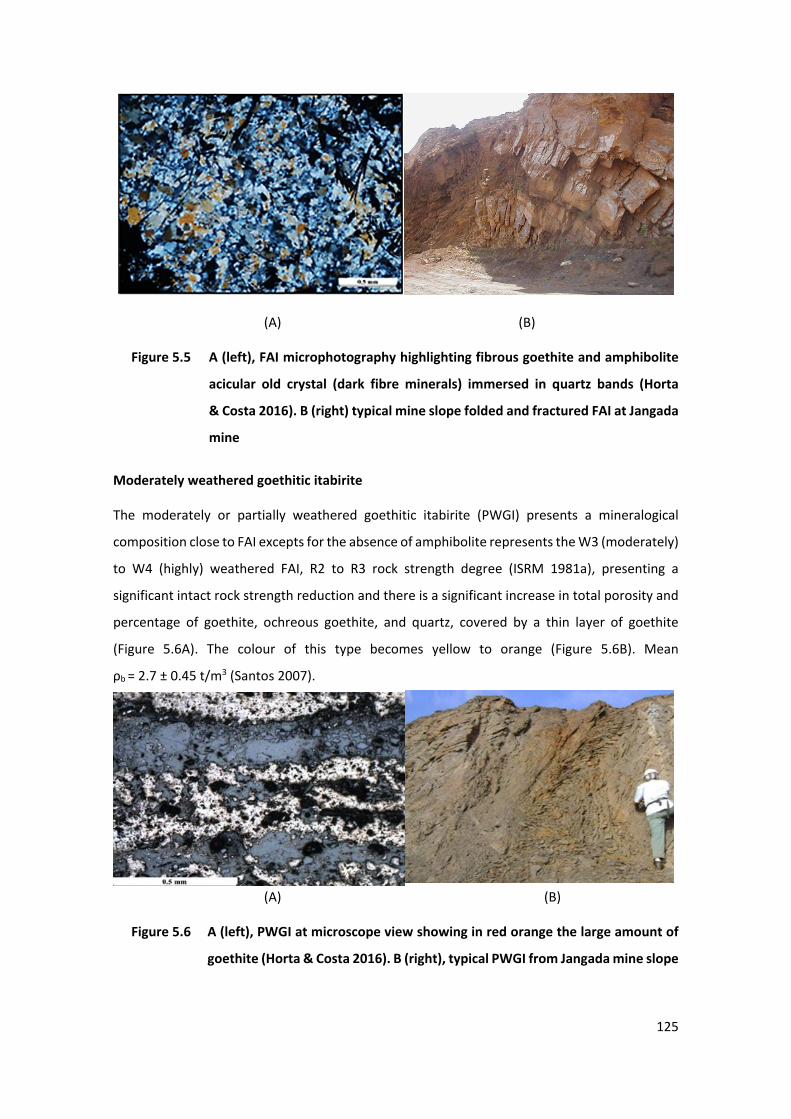
125
(A) (B)
28 Figure 5.5 A (left), FAI microphotography highlighting fibrous goethite and amphibolite
acicular old crystal (dark fibre minerals) immersed in quartz bands (Horta
& Costa 2016). B (right) typical mine slope folded and fractured FAI at Jangada
mine
Moderately weathered goethitic itabirite
The moderately or partially weathered goethitic itabirite (PWGI) presents a mineralogical
composition close to FAI excepts for the absence of amphibolite represents the W3 (moderately)
to W4 (highly) weathered FAI, R2 to R3 rock strength degree (ISRM 1981a), presenting a
significant intact rock strength reduction and there is a significant increase in total porosity and
percentage of goethite, ochreous goethite, and quartz, covered by a thin layer of goethite
(Figure 5.6A). The colour of this type becomes yellow to orange (Figure 5.6B). Mean
ρb = 2.7 ± 0.45 t/m3 (Santos 2007).
(A) (B)
29 Figure 5.6 A (left), PWGI at microscope view showing in red orange the large amount of
goethite (Horta & Costa 2016). B (right), typical PWGI from Jangada mine slope
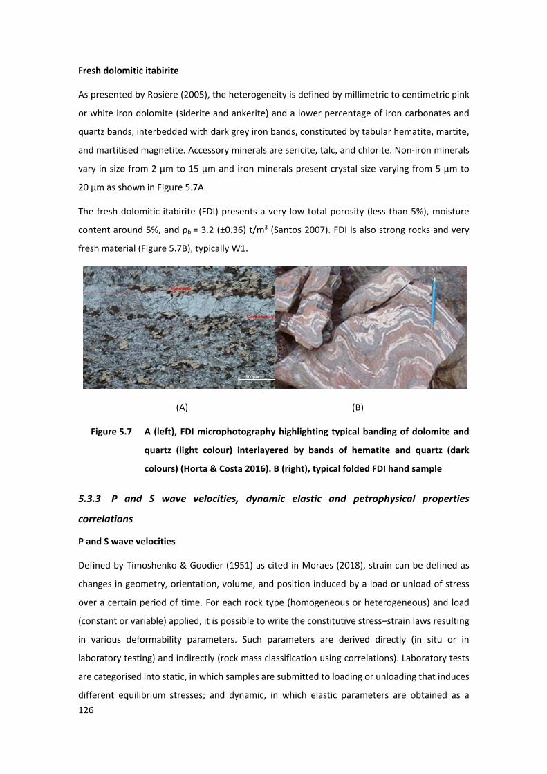
126
Fresh dolomitic itabirite
As presented by Rosière (2005), the heterogeneity is defined by millimetric to centimetric pink
or white iron dolomite (siderite and ankerite) and a lower percentage of iron carbonates and
quartz bands, interbedded with dark grey iron bands, constituted by tabular hematite, martite,
and martitised magnetite. Accessory minerals are sericite, talc, and chlorite. Non-iron minerals
vary in size from 2 µm to 15 µm and iron minerals present crystal size varying from 5 µm to
20 µm as shown in Figure 5.7A.
The fresh dolomitic itabirite (FDI) presents a very low total porosity (less than 5%), moisture
content around 5%, and ρb = 3.2 (±0.36) t/m3 (Santos 2007). FDI is also strong rocks and very
fresh material (Figure 5.7B), typically W1.
(A) (B)
30 Figure 5.7 A (left), FDI microphotography highlighting typical banding of dolomite and
quartz (light colour) interlayered by bands of hematite and quartz (dark
colours) (Horta & Costa 2016). B (right), typical folded FDI hand sample
5.3.3 P and S wave velocities, dynamic elastic and petrophysical properties
correlations
P and S wave velocities
Defined by Timoshenko & Goodier (1951) as cited in Moraes (2018), strain can be defined as
changes in geometry, orientation, volume, and position induced by a load or unload of stress
over a certain period of time. For each rock type (homogeneous or heterogeneous) and load
(constant or variable) applied, it is possible to write the constitutive stress–strain laws resulting
in various deformability parameters. Such parameters are derived directly (in situ or in
laboratory testing) and indirectly (rock mass classification using correlations). Laboratory tests
are categorised into static, in which samples are submitted to loading or unloading that induces
different equilibrium stresses; and dynamic, in which elastic parameters are obtained as a
500μm
127
response from a cyclic, rapid energy source such as acoustic wave emission that propagates the
rock material cyclically.
Using a laboratory test, as discussed at Kearey, et al. (2009), elastic modulus can be indirectly
obtained by calculating acoustic emission velocity (seismic waves) within the rock specimen, as
a result of particle vibration during energy release when triggered by an energy source. Such an
energy pulse is small, elastic, and independent of wave frequency. However, it differs from the
elastic modulus and material density and can be divided into two types: compressive waves or
P wave, that moves through the propagation direction (uniaxial strain), and shearing waves or
S wave, that moves perpendicular to the propagation path. The shear wave can be separated
into two polarised waves (horizontal and vertical), in relation to the transverse isotropy plane,
where the low velocity wave propagates perpendicular to the anisotropy plane (horizontal
polarisation) and the high velocity wave propagates parallel to the axis of anisotropy (vertical
polarisation).
Kearey et al. (2009) explain that wave velocity is also a function of the mineralogical
composition, texture, porosity, and presence of fluids. These factors severely affect the P wave
velocity (Vp), whereas the S wave velocity (Vs) did not propagate through discontinuities or
empty spaces. Several characteristics of Vp and Vs for common lithotypes are presented below:
• Felsic igneous rocks have lower velocities relative to mafic rocks.
• The velocity reduces as the rate of discontinuities (fractures) increases.
• Porous sedimentary rocks present velocity dispersion associated with the porosity and
density correlation, with higher velocities for high density and low porosity and lower
velocities for low density and high porosity. It also depends on the cementation grade,
consolidation, and other factors.
• Low velocities are registered for non-cohesive soils due to low crystal contact and high
porosity.
• In contrast with those with smaller crystals, lithotypes with the same mineral
composition but with larger crystals present higher velocities.
• The presence of fluids (water, oil, and air) filling pores (partially or completely)
representing a water pore pressure mainly influence the Vp. For high water pore
pressure, the velocities are higher when compared with low water pore pressure. For
low saturation degrees, the wave velocities are higher, while high saturation is lower.
128
In this context, the Vp is thus higher at rock matrix and lower at fluids and the air. The
Vs in the fluids generates minor changes as they do not generate shearing resistance.
• Higher wave velocity occurs parallel to the anisotropy direction and lower velocity is
observed in the direction perpendicular to anisotropy in metamorphic rocks. These
changes are associated with mineral and porous alignment, and the set of
discontinuities. Lower velocities are controlled by the weakness planes along banding
and schistosity. Otherwise, higher velocities are associated with the strongest crystal
contacts along the anisotropy direction.
• For the same reason, the Vp anisotropy decreases with stress and increases with
temperature. This effect may be due to the widening of pores and microcracks during
the expansion of the sample due to thermal stress.
Acoustic wave propagation velocity has been used to determine intact rock strength for several
typologies by researchers such as Inoue & Ohomi (1981) for weak rocks, Gaviglio (1989) for rock
density, Kaharaman (2001) and Yasar & Endogan (2004) for carbonate rocks. Based on their close
relation to the intact rock properties, structure, and texture, these methods were used by the
many mining companies in the world. Later studies and subsequent static tests (standard rock
strength tests) confirm static and dynamic comparisons (expressed with several formulas) with
the non-destructive laboratory test aspect of sonic wave measures. Furthermore, the low costs,
repeatability, and speed of acoustic emission tests are attractive characteristics.
Dynamic elastic waves that propagate through saturated or dry rock samples can be measured
in the laboratory by registering the transit time of each wave through the sample’s axial length
(Bourbié et al. 1987).
Classical rock mechanics provides various techniques for determining the elastic parameters,
the most widely employed being stress–strain curves that are obtained from destructive
compressive and tensile rock tests. Most recently, non-destructive tests based on acoustic wave
velocity propagation measures have been applied to obtain such parameters. The following are
benefits of using dynamic approaches: non-destructive, higher flexibility on sample geometry,
low cost, faster than destructive laboratory testing, and easier to perform the tests. Some
drawbacks can also be described, such as: obtained results are implicitly correlated with elastic
parameters and are directly related to the reliability of the database and the correlation curves
and equations used.
Additionally, acoustic emission can be coupled with laboratory static tests, facilitating constant
monitoring in different directions during the stress level increase.
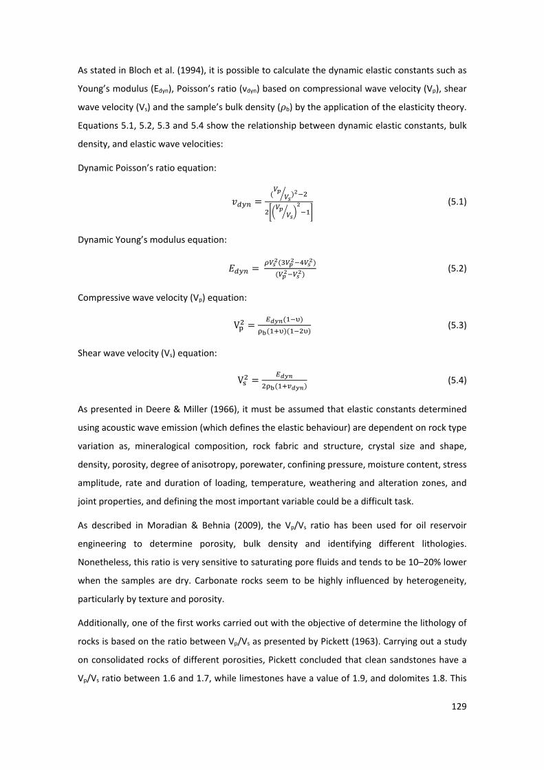
129
As stated in Bloch et al. (1994), it is possible to calculate the dynamic elastic constants such as
Young’s modulus (Edyn), Poisson’s ratio (νdyn) based on compressional wave velocity (Vp), shear
wave velocity (Vs) and the sample’s bulk density (𝜌𝜌b) by the application of the elasticity theory.
Equations 5.1, 5.2, 5.3 and 5.4 show the relationship between dynamic elastic constants, bulk
density, and elastic wave velocities:
Dynamic Poisson’s ratio equation:
𝑣𝑣𝑑𝑑𝑑𝑑𝑚𝑚 =(𝑉𝑉𝑝𝑝
𝑉𝑉𝑠𝑠� )2−2
2��𝑉𝑉𝑝𝑝
𝑉𝑉𝑠𝑠� �2−1�
(5.1)
Dynamic Young’s modulus equation:
𝐸𝐸𝑑𝑑𝑑𝑑𝑚𝑚 = 𝜌𝜌𝑉𝑉𝑠𝑠2(3𝑉𝑉𝑝𝑝2−4𝑉𝑉𝑠𝑠2)(𝑉𝑉𝑝𝑝2−𝑉𝑉𝑠𝑠2)
(5.2)
Compressive wave velocity (Vp) equation:
Vp2 = 𝐸𝐸𝑑𝑑𝑑𝑑𝑑𝑑(1−υ)ρb(1+υ)(1−2υ)
(5.3)
Shear wave velocity (Vs) equation:
Vs2 = 𝐸𝐸𝑑𝑑𝑑𝑑𝑑𝑑2ρb(1+𝑣𝑣𝑑𝑑𝑑𝑑𝑑𝑑)
(5.4)
As presented in Deere & Miller (1966), it must be assumed that elastic constants determined
using acoustic wave emission (which defines the elastic behaviour) are dependent on rock type
variation as, mineralogical composition, rock fabric and structure, crystal size and shape,
density, porosity, degree of anisotropy, porewater, confining pressure, moisture content, stress
amplitude, rate and duration of loading, temperature, weathering and alteration zones, and
joint properties, and defining the most important variable could be a difficult task.
As described in Moradian & Behnia (2009), the Vp/Vs ratio has been used for oil reservoir
engineering to determine porosity, bulk density and identifying different lithologies.
Nonetheless, this ratio is very sensitive to saturating pore fluids and tends to be 10–20% lower
when the samples are dry. Carbonate rocks seem to be highly influenced by heterogeneity,
particularly by texture and porosity.
Additionally, one of the first works carried out with the objective of determine the lithology of
rocks is based on the ratio between Vp/Vs as presented by Pickett (1963). Carrying out a study
on consolidated rocks of different porosities, Pickett concluded that clean sandstones have a
Vp/Vs ratio between 1.6 and 1.7, while limestones have a value of 1.9, and dolomites 1.8. This
130
ratio is independent of the density of the rock, whereas analysing only the speed of the Vp wave,
the lithology indicator could be considered ambiguous, since Vp is a function of other physical
rock properties as total porosity, mineralogy, and rock fabric.
Recent works from Motra & Stutz (2018) suggest that, for metamorphic anisotropic rocks (quartz
mica schist and amphibolite), the velocity anisotropy can be linked to the texture and anisotropy.
To determine the anisotropy effects, studies by Kern (1993); Punturo et al. (2005); and Motra &
Wuttke (2016) using S wave velocity propagation with different polarisation (parallel and
perpendicular), enables the determination of the amplitude of shear wave splitting, which is a
function of anisotropy, to measure the spatial dependency of wave velocities (anisotropy),
particularly for metamorphic rocks.
The work of Panakkal et al. (1990) showed a linear relationship between elastic moduli and
Poisson’s ratio with ultrasonic velocities, while testing sintered iron ore with porosity up to
21.6%, indicating that ultrasonic velocities (Vp and Vs) can be used for monitoring the elastic
moduli of porous materials without measuring density.
Petrophysical parameters
It is recognised, that other physical characteristics such as total porosity, bulk density,
mineralogical composition, crystal size, and fabric are directly responsible for variations in the
strength of intact rock. However, few studies of the interrelationship between intact rock
strength and petrophysical parameters have been established worldwide for BIF. Conclusions
from Thomson (1963) for Australian iron ores have suggested a theoretical hematite–quartz
curve used to determine the bulk density and appropriate iron content approximation.
Correlations presented by Aylmer et al. (1978) have associated bulk density, iron grade and
porosity for Mount Tom Price iron ore. Studies of Box & Reid (1976) for the iron ore formation
at Cockatoo Island, attempted to correlate true specific gravity with iron content and the
influence of porosity. Finally, studies by Nel (2007), developed for Sishen iron deposits in South
Africa, developed a direct correlation between porosity and dry bulk density, providing a reliable
calculation index.
Studies correlating dynamic elastic proprieties with petrophysical and static strength parameters
on BIF have been developed by Wassermann et al. (2009) for an oolithic iron mine in Lorraine,
France. The study evaluated damage processes on UCS tests using Vp and found that mechanical
behaviour deduced from strain measurements is dilatant for some samples and non-dilatant for
the others, even when elastic properties indicate damage processes for all samples.
131
Silva (2014), studying rocks Archean schists from Cuiabá mine, Brazil had measured permeability
and total porosity and elastodynamic properties that show the rigidity of these rocks and can be
used to define lithostructural constraints.
For iron oxide mineralisation in the Blötberget mine, Sweden, Maries et al. (2017), obtained
several physical properties from geophysical logging and laboratory measurements to assess the
ore-bearing rocks by increasing density and dynamic elastic modules measured from the full
waveform sonic.
For BIF in the Iron Quadrangle, the studies of Pereira (2017) using acoustic emission and other
geophysical techniques on well logging, defined rock strength parameters and discontinuity
characteristics to establish rock quality designation (RQD) and elastic in situ modules. Moraes
(2018), using part of this research database, evaluated, and correlated dynamic and static
proprieties in different anisotropy directions using statistical approaches. The author has shown
a well-adjusted regressive model for fresh itabirites. In general, the levels of the statistical
parameters are improved for initial anisotropy directions with a poorly adjusted regression
curve after the elimination of spurious data.
Bulk density is the most direct and easy-to-measure indicator of changes in compactness and level
of alteration of a sample (Van den Akker & Soares 2005). It is an essential physical property, which
has good correlation with the majority of index properties of rock, mainly with P wave porosity.
For Brazilian BIF, studies by Ribeiro et al. (2014), Santos et al. (2005), and Santos (2007) focused
on evaluating the association between bulk density and iron content for Vale’s iron ore mines
and concluded that there is a linear positive correlation between the total iron ore content and
the bulk density.
Anisotropy and heterogeneity
BIF heterogeneity is an important geological characteristic easily observed and measured on
several scales varying from a few millimetres to several centimetres and is defined by typical
metamorphic banding. This heterogeneity can result in an anisotropy described as transverse
isotropy, in which layers have approximately the same rock properties along the plane of the
band and different rock properties across the band. As suggested by Hudson & Harrison (2000),
geomechanically, the important rock properties that can be affected by anisotropy are
deformability modulus, strength, brittleness, permeability, and discontinuity frequency.
Singh (1989) and Ramamurthy (1993) pointed out that metamorphic rocks are mostly
anisotropic due to the effect of schistosity, cleavage and microcracking. For BIF, anisotropy is
132
defined by its mineralogical composition (metamorphic banding), mineralogical orientation
(alignment of minerals at the same orientation), the porosity induced by the original
composition or weathering, and different bulk densities in each layer. Additionally, secondary
anisotropy directions, defined by schistosity and foliation, are locally found mainly in hematitites
and in itabirites with some discreet shear zones, and fold axes.
The compositional metamorphic banding and heterogeneity are defined by the alternation of iron
and non-iron layers (typical itabiritic compositional metamorphic banding) and is defined in the
research as ’heterogeneity’. It is the most important itabirite feature that dictates the formation
of the intact rock strength, and is controlled by iron or non-iron layer thickness, porosity, and
mineral composition. A simple example is observed in zones where the banding contains thicker
layers of iron minerals, the itabirite will be denser, with lower porosity, relatively higher strength
values and richer in iron content.
It is expected for BIF to behave like an anisotropic material, where physical properties present
symmetric characteristics about an axis normal to compositional metamorphic banding, which
is the plane of isotropy. However, this compositional metamorphic banding also defines itabirite
heterogeneity (bands of iron minerals intercalated with non-iron mineral layers).
Ultimately, BIF heterogeneity is responsible for determining the different lithotypes, ranging
from country rocks such as dolomite, quartzite, and amphibolite (very few or non-iron bands) to
high-grade ore (very few or no waste bands) as rich itabirite or hematitite. This evaluation is
consistent with results presented by Dalstra et al. (2003) that compare the Hamersley Province
iron ore with many global deposits and correlate the proto-ore assemblages with intermediate
Fe-grades between ore and the host BIF.
For Saroglou & Tsiambaos (2007), the engineering behaviour of rock masses is strongly
dependent on the anisotropy present at different scales. At the microscale (intact rock) it
depends on the alignment of the rock crystals (i.e., inherent anisotropy). At the macroscale (rock
masses) with anisotropic structure, it is characterised by distinct bedding or schistosity planes
(structural anisotropy). The anisotropy of intact rock, which is the focus of this chapter, can be
determined by the variation of the velocity anisotropy index (IVp) as proposed by Saragou &
Tsiambaros (2007) due to the existence of bedding, foliation and schistosity planes in both intact
rock observed at the macroscale and microscale.
133
5.4 METHODOLOGY
To evaluate fresh and moderately weathered BIF, its petrophysical and geotechnical
characteristics, and achieve the proposed goals, the methodology was divided into three phases,
as described below.
The first phase included field investigations, in which several samples were collected from
surface outcrops and core drills, covering all BIF lithotypes. Geological and geotechnical
information, based on ISRM (1981) suggestions, were collected, and outcrops and samples were
photographed for additional visual information and physical parameter recognition
(e.g. anisotropy, banding, type of BIF, discontinuities, and mineralogy).
The second phase focused on petrographic thin section analyses, used to evaluate rock
mineralogy, fabric, and porosity, to provide information from a microscopy point of view and
compare it with field macro characteristics.
The third phase included undertaking and evaluating all laboratory tests used to determine the
dynamic intact rock properties, and correlations between the petrophysical characteristics and
geotechnical parameters of each BIF type. Correlations between anisotropy, ρb, Vp and Vs
velocity, Poisson's dynamic ratio, and Young's dynamic modulus were chosen as these rock
properties are considered to be the ones that play a role in the slope stability design and
evaluation for these types of rocks.
The sampling validation approach presented by Appendix I was used to reduce parameter
variability due to geological effects and defects. High variance is also motivated by intrinsic
sample variation or negligence during sample selection and grouping. Samples were grouped by
geological characteristics such as banding type, type of BIF, anisotropy direction on samples,
bulk density, and the presence of geological features, to reduce the variance and provide a
better lithotype identification.
The methodology proposed to cross-check pre-test samples was:
• Samples were grouped by level of weathering, W1 and W2 for fresh and W3 and W4
for moderately weathered, based on ISRM (1981).
• Vp measurements were used to discard inadequate samples (containing inclusions or
microfractures).
• As presented in Ribeiro et al. (2014) and Appendix I the BIF present a typical bulk
density range, and this range was used to separate fresh itabirites, ranging from
134
2.7 t/m3 to 3.8 t/m3 from non-iron or waste rock with ρb below 2.7 t/m3 and hematitite
with ρb above 3.8 t/m3.
• All samples were photographed before and after tests to find the main geological
characteristics, failure surface and failure mode.
• As presented in Appendix I, some geological features such as intense folding, the
presence of specularite levels, filling material with a different weathering degree,
quartz, and calcite veins are the main features that do not represent the typical
itabirites heterogeneity and for this reason were not evaluated.
• Itabirites samples that did not show typical banding were not evaluated.
Extreme outlier results were removed according to the box plot statistical methodology
(Whitaker et al. 2013). This technique identifies the mild outlier’s values from the quartiles (Qt)
determination, based on Equation 5.5.
Values below the lower inner fence (QtLower):
QtLower = 1Qt - 1.5(3Qt - 1Qt) (5.5)
and values above the upper inner fence (Qtupper) as Equation5.6:
Qtupper = 3Qt + 1.5(3Qt - 1Qt) (5.6)
where 1Qt is the first quartile and 3Qt is the third quartile.
The 3Qt evaluates database dispersion around a central data leaving 75% of data below the sum
and is defined by Equation 5.7:
3Qt = × + 1.5.IQR (5.7)
The first or inferior quartile (1Qt) evaluates database dispersion around a central data leaving
25% of data below the sum and is defined by Equation 5.8.
1Qt = × - 1.5.IQR (5.8)
Interquartile ranges (IQR) measure how spread out from a central data the values are and these
form what are called outliers and are defined by Equation 5.9:
IQR = 3Qt - 1Qt (5.9)
For BIF which present metamorphic heterogeneity in a determinate scale of observation, it is
necessary to determine the ratio of anisotropy to evaluate the degree of anisotropy. Estimating
the variation of each parameter due to the effect of anisotropy allows the differentiation of
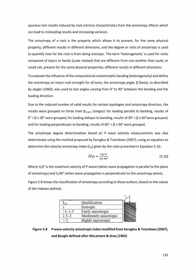
135
spurious test results induced by rock intrinsic characteristics from the anisotropy effects which
can lead to misleading results and increasing variance.
The anisotropy of a rock is the property which allows it to present, for the same physical
property, different results in different directions, and the degree or ratio of anisotropy is used
to quantify how far the rock is from being isotropic. The term ‘heterogeneity’ is used for rocks
composed of layers or bands (scale related) that are different from one another that could, or
could not, present for the same physical properties, different results in different directions.
To evaluate the influence of the compositional metamorphic banding (heterogeneity) and define
the anisotropy on intact rock strength for all tests, the anisotropy angle, β (beta), as described
by Jaeger (1960), was used to test angles varying from 0° to 90° between the banding and the
loading direction.
Due to the reduced number of valid results for certain typologies and anisotropy direction, the
results were grouped on three main βangles (ranges): for loading parallel to banding, results of
0° < β ≤ 30° were grouped; for loading oblique to banding, results of 30° < β ≤ 60°were grouped;
and for loading perpendicular to banding, results of 60° < β ≤ 90° were grouped.
The anisotropy degree determination based on P wave velocity measurements was also
determinate using the method proposed by Saroglou & Tsiambaos (2007), using an equation to
determine the velocity anisotropy index (Ivp) given by the ratio presented in Equation 5.10.
𝐼𝐼𝐼𝐼𝐼𝐼 = 𝑉𝑉𝑉𝑉 0°𝑉𝑉𝑉𝑉 90°
(5.10)
Where Vp0° is the maximum velocity of P waves (when wave propagation is parallel to the plane
of anisotropy) and Vp90° (when wave propagation is perpendicular to the anisotropy plane).
Figure 5.8 shows the classification of anisotropy according to these authors, based on the values
of the indexes defined.
31 Figure 5.8 P wave velocity anisotropic index modified from Saroglou & Tsiambaos (2007),
and βangle defined after McLamore & Gray (1962)
136
A pragmatic solution has been suggested by Chang et al. (2006) where a number of empirical
relations have been proposed for linking dynamic rock strength with physical and geological
parameters. In many situations, using such relationships is often the only way to estimate static
strength due to the absence of laboratory testing cores. The basis for these interactions is that
many of the same factors that affect rock strength also affect other physical properties, including
wave velocity, elastic moduli, bulk density, Poisson’s ratio, and porosity. This chapter shows how
good this correlation is for two sets of data that are strongly linked together. Further, an
adequate coefficient of correlation that describes the strength and the direction of the
correlations of the variables must be shown in order to measure and determine the relationship
between two variables.
According to Butel et al. (2014), the quality of the correlation is determined by the values of the
coefficient of determination (R2) value, the size of the dataset, and the visual fit of the regression
curve. During correlation evaluation analysis, tested several adjusted fitting curves (e.g. linear,
exponential, and potential) were tested. The exponential adjustment curve proved to be the
most suitable curve for the available dataset, even when some correlation proves to be better
for linear or potential regressions (e.g. the correlation ratios obtained were not significantly
different from the exponential values). The correlation coefficient has been calculated by using
the ‘best fitting’ approach using automatic procedures through several attempts on the dataset.
The exponential adjusted curve is defined as the curve best fitted to evaluate the variables,
correlations, and dispersions, and define the adjusted equation which gives the proportion of
the variance in the independent variables. In other words, the R2 is a measure of how well a
regression curve matches a set of data for an evaluated dataset. It could also be interpreted as
the adjusted model of observed effects between two dependent variables, with the strength of
the correlation is defined as 0 to 0.29 (little if any correlation), 0.3 to 0.49 (low), 0.5 to 0.69
(moderate), 0.7 to 0.89 (high) and 0.9 to 1.0 (very high correlation) as presented in Asuero et al.
(2006).
Due to the material characteristics and the lack of bibliographic references for studied rock
types, the adequate correlation ratio was considered to be equal or superior to 0.50 (moderate).
5.4.1 Laboratory tests
For hard strength, fresh to moderately weathered lithotypes, elastic parameters (dynamic
Young’s modulus (Edyn) and Poisson’s ratio (νdyn)), were defined based on Vp and Vs, used not only
to determine the parameters but also to evaluate the integrity of the samples. Bulk density (ρb)
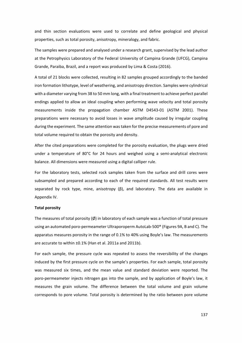
137
and thin section evaluations were used to correlate and define geological and physical
properties, such as total porosity, anisotropy, mineralogy, and fabric.
The samples were prepared and analysed under a research grant, supervised by the lead author
at the Petrophysics Laboratory of the Federal University of Campina Grande (UFCG), Campina
Grande, Paraiba, Brazil, and a report was produced by Lima & Costa (2016).
A total of 21 blocks were collected, resulting in 82 samples grouped accordingly to the banded
iron formation lithotype, level of weathering, and anisotropy direction. Samples were cylindrical
with a diameter varying from 38 to 50 mm long, with a final treatment to achieve perfect parallel
endings applied to allow an ideal coupling when performing wave velocity and total porosity
measurements inside the propagation chamber ASTM D4543-01 (ASTM 2001). These
preparations were necessary to avoid losses in wave amplitude caused by irregular coupling
during the experiment. The same attention was taken for the precise measurements of pore and
total volume required to obtain the porosity and density.
After the cited preparations were completed for the porosity evaluation, the plugs were dried
under a temperature of 80°C for 24 hours and weighed using a semi-analytical electronic
balance. All dimensions were measured using a digital calliper rule.
For the laboratory tests, selected rock samples taken from the surface and drill cores were
subsampled and prepared according to each of the required standards. All test results were
separated by rock type, mine, anisotropy (β), and laboratory. The data are available in
Appendix IV.
Total porosity
The measures of total porosity (Ø) in laboratory of each sample was a function of total pressure
using an automated poro-permeameter Ultraporoperm AutoLab-500® (Figures 9A, B and C). The
apparatus measures porosity in the range of 0.1% to 40% using Boyle’s law. The measurements
are accurate to within ±0.1% (Han et al. 2011a and 2011b).
For each sample, the pressure cycle was repeated to assess the reversibility of the changes
induced by the first pressure cycle on the sample’s properties. For each sample, total porosity
was measured six times, and the mean value and standard deviation were reported. The
poro-permeameter injects nitrogen gas into the sample, and by application of Boyle’s law, it
measures the grain volume. The difference between the total volume and grain volume
corresponds to pore volume. Total porosity is determined by the ratio between pore volume
138
and total volume. Once the sample is dried, it is possible to assume that the solid sample mass
corresponds to the total mass previously measured.
A visual total porosity (Øb) was also determined using petrographical thin sections qualitative
visual determination. The comparation between total porosity (poro-permeameter measured)
and visual total porosity (thin sections evaluations) must be compared with restriction due to
the nature of measures.
(A) (B) (C)
32 Figure 5.9 A (left), poro-permeameter pressure gauges. B (centre), pressure
transductors. C (right), compression chamber (Lima & Costa 2016)
Bulk density
In this chapter, bulk density was determined according to the ratio between total dry mass and
total volume using standards outlined in ASTM 1289.6.4.1 (AS 2016) for the Australian
laboratory and ABNT NBT 6508 (ABNT 1989) for the Brazilian laboratory. The bulk density of
each specimen is calculated according to Equation 5.8:
ρb = M/V (5.8)
Where ρb is the bulk density (kg/m3), M is the mass of the specimen measured prior to testing
(kg), and V is the volume (m3) of the specimen, calculated from dimensions measured during
sample preparation.
Additionally, using the Ultraporoperm 500 ® it was also possible to obtain the grain density given
by the ratio between total mass of the sample and grain volume. Once porosity and grain density
were obtained, bulk density was estimated, neglecting density of air, which fills samples’ voids.
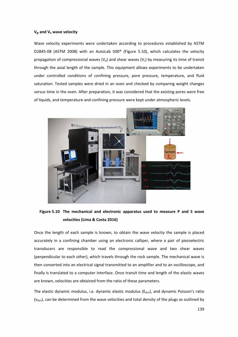
139
Vp and Vs wave velocity
Wave velocity experiments were undertaken according to procedures established by ASTM
D2845-08 (ASTM 2008) with an AutoLab 500® (Figure 5.10), which calculates the velocity
propagation of compressional waves (Vp) and shear waves (Vs) by measuring its time of transit
through the axial length of the sample. This equipment allows experiments to be undertaken
under controlled conditions of confining pressure, pore pressure, temperature, and fluid
saturation. Tested samples were dried in an oven and checked by comparing weight changes
versus time in the oven. After preparation, it was considered that the existing pores were free
of liquids, and temperature and confining pressure were kept under atmospheric levels.
33 Figure 5.10 The mechanical and electronic apparatus used to measure P and S wave
velocities (Lima & Costa 2016)
Once the length of each sample is known, to obtain the wave velocity the sample is placed
accurately in a confining chamber using an electronic calliper, where a pair of piezoelectric
transducers are responsible to read the compressional wave and two shear waves
(perpendicular to each other), which travels through the rock sample. The mechanical wave is
then converted into an electrical signal transmitted to an amplifier and to an oscilloscope, and
finally is translated to a computer interface. Once transit time and length of the elastic waves
are known, velocities are obtained from the ratio of these parameters.
The elastic dynamic modulus, i.e. dynamic elastic modulus (Edyn), and dynamic Poisson’s ratio
(νdyn), can be determined from the wave velocities and total density of the plugs as outlined by
140
Bourbié et al. (1987), Sheriff (1991), and Soares (1992) using Equations 5.1, 5.2, 5.3 and 5.4
presented in the previous section.
It must be noted that the best sonic couplings achieved to produce reliable P and S wave results
were obtained mostly for fresh typologies. Good coupling was not achieved for moderately
weathered materials. For this reason, these lithotypes were clustered in some analyses with
PWQI and PWGI because of the low amount of reliable results and the geological and
geotechnical similarities.
Petrographic thin sections description
Several thin sections were prepared perpendicular to the bedding plane and the main
characteristics observed were visual total porosity (Øb), grain and pore size, shape distribution,
mineralogy, and fabric. The data were used to validate in microscale some features observed on
the macroscale, including heterogeneity, anisotropy, total porosity, and mineral distribution.
A total of 33 thin sections were prepared and evaluated. The sections were produced by The
University of Western Australia (UWA) petrography laboratory, and the description and
percentage measures were undertaken under an Australian Centre for Geomechanics (ACG)
research grant, supervised by the author’s supervisor and presented in Horta & Costa (2016).
5.5 RESULTS
5.5.1 Mineralogical and fabric overview
Mineralogy is based on BIF origin and fabric is associated with tectonical settings (regional and
local) and metamorphism. It is highly affected by the weathering process and redefined by the
weathering grade.
The mineralogical ensemble, textural characteristic (rock fabric) and total porosity are important
characteristics used to define the anisotropic behaviour and geomechanical properties for the
BIF. The analyses for FQI, FDI, FAI, PWGI and PWQI were supported using field investigations
and were used in conjunction with microscopic evaluations from Horta & Costa (2016). For HHE,
as there is a vast literature review available related to its fabric and mineralogical composition,
studies by Rosière et al. (1996 and 2001), Varajão et al. (2002) and Spier et al. (2003) were used.
As suggested by Baars & Rosiére (1997) and Rosière et al. (2001), the BIF fabric at the western
side of the Iron Quadrangle can be separated into three major domains: a subhedral to euhedral
crystals domain, with an overall granoblastic fabric, defined as the most common type and
considered to represent post-tectonic partial recrystallisation; a euhedral domain of locally
141
tabular-shaped or very elongated specularite platelets, preferred orientation, defining a
secondary schistosity induced by shearing and a high stress domain; and a locally brecciaed
fabric domain, that can be induced by tectonical or physical collapse zones.
Such domains reflect distinct microcharacteristics that are not always noticed on the
macroscale. These domains were associated with the three geological settings identification on
this research that influence the geomechanical and anisotropic behaviour:
• Post-tectonical domain (weathering), characterised by the complete mineral leaching
or mineral boundary contact leaching.
• Tectonical high stress zones, describing orientated mineral assemblage.
• Brecciated zone (weathering or tectonical), with porous level either orientated or not.
Table 5.1 shows summary results for 33 thin sections presenting the name and percentage of
the main constituent minerals, and maximum and minimum crystal size (between brackets).
Also presented are the visual total porosity percentage, and maximum and minimum size
(between brackets) of pores for three types of measures. Intragranular pores correspond to the
percentage of pores inside crystals generally not interconnected. Intergranular pore
corresponds to porosity between crystals and are generally interconnected. Secondary pore
refers to fracture pore percentage. The visual total porosity (Øb) is the sum of the three pores’
percentage and was considered the maximum total percentage. For Øb in brackets, the minimum
value does not consider the secondary pores (intact rock) and for maximum value, the secondary
pore is included.
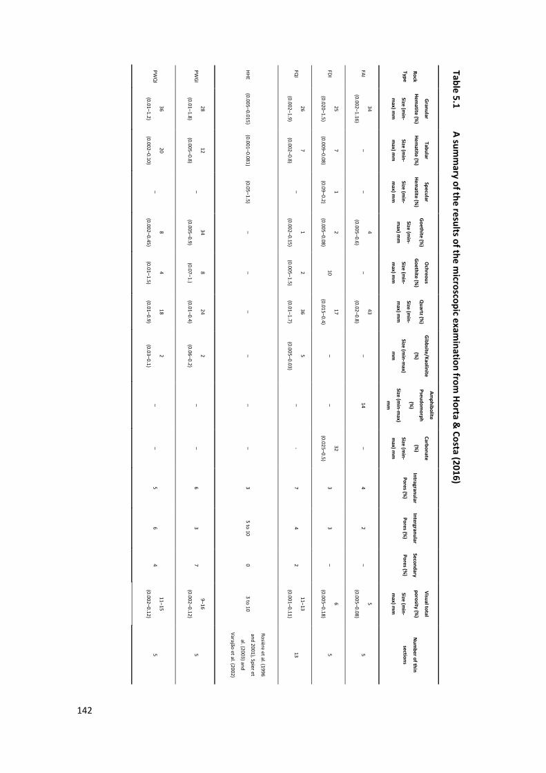
8Table 5.1 A sum
mary of the results of the m
icroscopic examination from
Horta &
Costa (2016)
Rock
Type
Granular
Hematite (%
)
Size (min-
max) m
m
Tabular
Hematite (%
)
Size (min-
max) m
m
Specular
Hematite (%
)
Size (min-
max) m
m
Goethite (%
)
Size (min-
max) m
m
Ochreous
Goethite (%
)
Size (min-
max) m
m
Quartz (%
)
Size (min-
max) m
m
Gibbsite/Kaolinite
(%)
Size (min-m
ax)
mm
Amphibolite
Pseudomorph
(%)
Size (min-m
ax)
mm
Carbonate
(%)
Size (min-
max) m
m
Intragranular
Pores (%)
Intergranular
Pores (%)
Secondary
Pores (%)
Visual total
porosity (%)
Size (min-
max) m
m
Num
ber of thin
sections
FAI 34
(0.002–1.16) –
– 4
(0.005–0.6) –
43
(0.02–0.8) –
14 –
42
– 5
(0.005–0.08) 5
FDI 25
(0.020–1.5)
7
(0.009–0.08)
1
(0.09–0.2)
2
(0.005–0.08) 10
17
(0.015–0.4) –
– 32
(0.025–0.5) 3
3 –
6
(0.005–0.18) 5
FQI
26
(0.002–1.9)
7
(0.002–0.8) –
1
(0.002–0.15)
2
(0.005–1.5)
36
(0.01–1.7)
5
(0.005–0.03) –
-7
4 2
11–13
(0.001–0.11) 13
HHE (0.005–0.015)
(0.001–0.081) (0.05–1.5)
– –
– –
– –
3 5 to 10
0 3 to 10
Rosière et al. (1996
and 2001), Spier et
al. (2003) and
Varajão et al. (2002)
PWGI
28
(0.01–1.8)
12
(0.005–0.8) –
34
(0.005–0.9)
8
(0.07–1.)
24
(0.01–0.4)
2
(0.06–0.2) –
– 6
3 7
9–16
(0.002–0.12) 5
PWQ
I 36
(0.01–1.2)
20
(0.002–0.10) –
8
(0.002–0.45)
4
(0.01–1.5)
18
(0.01–0.9)
2
(0.03–0.1) –
– 5
6 4
11–15
(0.002–0.12) 5
142
143
In general, the analyses of these thin sections indicated three main characteristics of pervasive
fabric responsible for inducing penetrative planes that could represent heterogeneity and result
in rock anisotropy:
• Band boundary contacts between layers with different mineral compositions, defining
the compositional metamorphic banding; mainly quartz for FQI, PWQI, FAI, PWGI, and
carbonates for FDI. This characteristic is not observed for HHE as it is a monomineralic
rock.
• Planar or granular minerals orientated in one direction (mineral orientation), defined
by tabular hematite and recrystalised quartz and carbonate crystals.
• Orientated porous layers (pore orientation), defined by orientated intergranular pores
aligned along the metamorphic banding (band boundary and mineral orientation) or
along discontinuities. This characteristic defines the metamorphic banding for HHE.
It is noted in Table 5.1 that fresh or moderately weathered BIF presented no significant changes
in crystal or pores size; the main changes are the increase in goethite, tabular hematite,
ochreous goethite and presence of kaolinite and gibbsite not seen in fresh types and total
porosity percentage increase from fresh to moderately weathered types. The anisotropy
observed in these rocks could be associated with these characteristics and not with the rock
fabric (mineral orientation) that generally are responsible for anisotropic effects.
It is noted that Øb increases from fresh (5% to 13%) to moderately weathered (9% to 16%) on
average. This increase is attributed to mineral leaching and alteration of iron and non-iron bands
highly affected by the degree of weathering. Additionally, FQI presented higher Øb from 11% to
13% comparing with other fresh BIF, this difference can be attributed to the presence of slightly
weathered thin sections that could influence the results.
A description of each lithotype is presented below.
Fresh to slightly weathered quartzitic itabirite
Fresh quartzitic itabirite (FQI) mineralogy is marked by the presence of quartz, granular
hematite, tabular hematite, goethite, and ochreous goethite. Kaolinite and gibbsite occur as
accessory minerals.
The presence of a slightly weathered portion is observed by the higher percentage of goethite
and ochreous goethite as small crystals in quartz rich bands, and anhedral shapes can also occur
filling pores. Bands of quartz have higher Øb = 20%, mainly resulting from intergranular pores. In
144
these bands where microplates of hematite occur in larger quantities the porosity is slightly
smaller.
Bands of hematite present lower Øb = 7% but with the presence of lobed crystals, tabular
hematite crystals larger than 0.80 mm and granular hematites larger than 1.3 mm in some zones
Øb can reach 30%. Hematite crystals lower than 1.3 mm were considered part of the banding
itself.
In general, FQI presented higher Øb from 11% to 13% compared to another fresh BIF. This
difference can be attributed to the presence of slightly weathered thin sections that could
influence the results.
Fresh amphibolitic itabirite
Fresh amphibolitic itabirite (FAI) mineralogy is mainly defined by the presence of quartz,
hematite, goethite as a pseudomorph of amphibolite, goethite, and ochreous goethite. The
pseudomorph of amphibolite is generally altered to fibrous goethite and only occurs in some of
the thin sections. Goethite usually occurs with an anhedral shape in between quartz crystals (as
a cement) but also as crystals.
Quartz bands are well preserved and large hematite crystals (1.1 mm) were interpreted as being
part of the preserved hematite band. Hematite bands present lower total porosity and the limits
between quartz and hematite bands are not very clear due to the pore distribution and lower
concentration in the boundaries as observed in FQI.
Ochreous goethite, gibbsite and kaolinite occur as accessory minerals. All the samples present
low Øb (5%).
Fresh dolomitic itabirite
Fresh dolomitic itabirite (FDI) mineralogy is defined by the presence of hematite, iron dolomite,
quartz, goethite, and ochreous goethite. Granular hematite is predominant and has its size
decreased when iron dolomite (ankerite and siderite) occurs in higher quantities. Iron dolomite
occurs as granuloblastic crystals interlayered with hematite bands, as well as filling spaces
between crystals (calcite). Ochreous goethite occurs as cement, filling spaces between crystals of
hematite and crystals of calcite. Its occurrence is better observed in the boundaries of hematite
bands where carbonate and crystals of hematite in smaller size dominate.
Quartz is present in bands where crystals and sub-crystals are orientated. Talc occurs as an
accessory mineral.
145
FDI presents a low Øb of 6%. Bands of hematite also present some percentage of iron dolomites
and are characterised by relatively lower Øb. In this band, hematite occurs as granular and/or
tabular crystals and iron dolomites as a matrix with very fine crystals. For iron dolomite bands,
the percentage and intergranular pores are considerably larger.
Hard hematitite
From Rosière et al. (1996 and 2001) and Varajão et al. (2002) and Spier et al. (2003), the hard
hematitite (HHE) is constituted mainly of iron oxides and hydroxides (e.g. hematite and martite)
with the percentage of pores between 3% and 10% (Table 5.1). The heterogeneous
metamorphic banding is represented by layers with higher porosity interlayered with more
massive ones, conditioned by mineral and pore orientation. In addition, in shallower depths for
slightly weathered types these porous layers became a preferential patch for weathering
(oxidation of iron minerals) increasing anisotropy effects and weakness of this band. Locally, the
presence of specularite can induce a higher anisotropy degree.
Moderately weathered quartzitic itabirite
The moderately or partially weathered quartzitic itabirite (PWQI) mineralogy is characterised by
hematite, quartz, goethite, and kaolinite, ochreous goethite, and gibbsite in a smaller percentage.
Hematite is characterised by crystals with low intergranular porosity and some pores can be
partially to completely filled with goethite or ochreous goethite as cement. In general, kaolinite
and gibbsite appear filling intragranular pores. Quartz bands and hematite bands were hardly
identified, and bands of hematite present lower relative total porosity and quartz bands have
higher relative total porosity. However, this is reduced when goethite is filling the space (cement)
between quartz and hematite. For this reason, the Øb varies from 11% to 15%.
Moderately weathered goethitic itabirite
Moderately or partially weathered goethitic itabirite (PWGI) is characterised by hematite,
goethite, quartz, ocherous goethite, and gibbsite and kaolinite occur in smaller percentage.
Anhedral goethite or ochreous goethite are common in spaces between crystals of quartz and
hematite (cement). However, they are also observed as a crystal in smaller concentrations.
Hematite is present as lobed crystals and microplates.
Bands of hematite present lower relative total porosity. Quartz bands have a higher relative total
porosity. However, this is reduced when goethite is filling the space (cement) between quartz
and hematite. For this reason, the Øb varies from 9% to 16%.
146
The main difference between PWQI and PWGI is the increase of goethite and ochreous goethite,
and the consequent hematite reduction for PWGI. The PWGI total porosity seems to be relatively
lower due to the goethitic cementation. However, evaluated thin sections did not confirm this
field observation.
5.5.2 Heterogeneity and anisotropy evaluations
It is expected for heterogeneity promoted by typical compositional metamorphic banding of the
BIF to be responsible for a transversal isotropy. Analysis conducted on this research showed at
least three different types of fabric characteristics that could induce heterogeneity, which could
induce anisotropy.
Analyses conducted in Section 5.5.1, found three main characteristics of pervasive fabric that
could be responsible for inducing penetrative planes representing heterogeneity and resulting
in rock anisotropy: boundary contacts between layers with different mineral composition,
defining the compositional metamorphic banding; planar or granular minerals orientated
according to one direction (mineral orientation); and orientated porous levels (pore
orientation).
The heterogeneity observed in itabirites is different from that observed in hematitites, however
both satisfy the heterogeneity characteristic defined by Amann et al. (2013) which states that
they visually appear heterogeneous, with evidence of non-uniform crystal size distribution at
the specimen scale, variable mineral grain composition and total porosity.
Bands boundary contact
For fresh itabirites, millimetric to centimetric bands with different mineralogy (e.g. hematite,
quartz, or iron dolomite) define an itabirite heterogenous compositional metamorphic banding.
While evaluating itabirite fabric under a microscope, one can observe relative higher differences
in crystal sizes (0.002 mm to 1.9 mm) for iron bands and smaller differences (0.01 mm to 1.7 mm)
for non-iron bands representing a high roughness due to the size difference, as shown in Figure
5.11A.
The band boundary is defined for hard hematitite by millimetric to centimetric banding
alternation of different iron minerals (e.g. granular hematite, martite or microplates of
hematite) each mineral can present different crystal sizes. Its supported by Varajão et al. (2002)
defined for this type, crystal sizes varying from 10 μm to 30 μm for hematite and martite granular
crystals, and 1 μm for microplates of hematite. The contact between these minerals (boundary
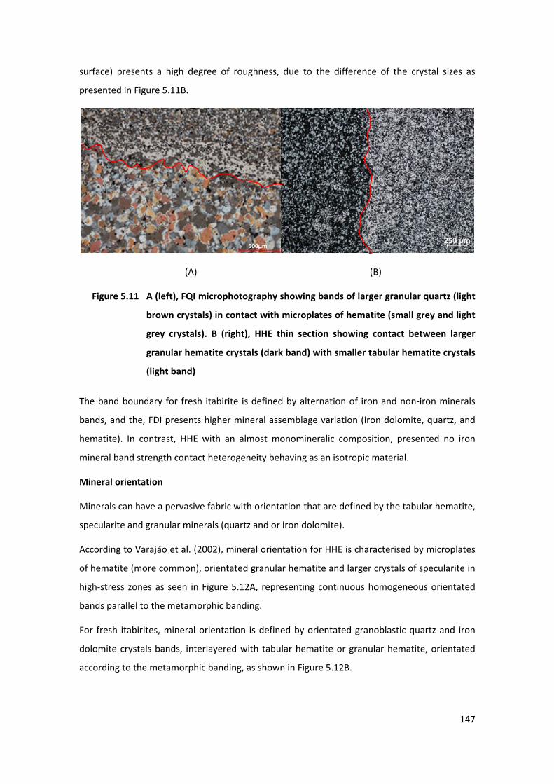
147
surface) presents a high degree of roughness, due to the difference of the crystal sizes as
presented in Figure 5.11B.
(A) (B)
34 Figure 5.11 A (left), FQI microphotography showing bands of larger granular quartz (light
brown crystals) in contact with microplates of hematite (small grey and light
grey crystals). B (right), HHE thin section showing contact between larger
granular hematite crystals (dark band) with smaller tabular hematite crystals
(light band)
The band boundary for fresh itabirite is defined by alternation of iron and non-iron minerals
bands, and the, FDI presents higher mineral assemblage variation (iron dolomite, quartz, and
hematite). In contrast, HHE with an almost monomineralic composition, presented no iron
mineral band strength contact heterogeneity behaving as an isotropic material.
Mineral orientation
Minerals can have a pervasive fabric with orientation that are defined by the tabular hematite,
specularite and granular minerals (quartz and or iron dolomite).
According to Varajão et al. (2002), mineral orientation for HHE is characterised by microplates
of hematite (more common), orientated granular hematite and larger crystals of specularite in
high-stress zones as seen in Figure 5.12A, representing continuous homogeneous orientated
bands parallel to the metamorphic banding.
For fresh itabirites, mineral orientation is defined by orientated granoblastic quartz and iron
dolomite crystals bands, interlayered with tabular hematite or granular hematite, orientated
according to the metamorphic banding, as shown in Figure 5.12B.
500μm
500μm
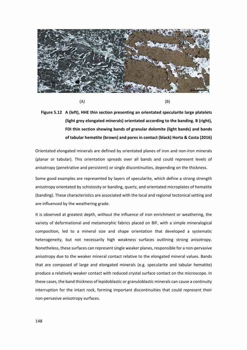
148
(A) (B)
35 Figure 5.12 A (left), HHE thin section presenting an orientated specularite large platelets
(light grey elongated minerals) orientated according to the banding. B (right),
FDI thin section showing bands of granular dolomite (light bands) and bands
of tabular hematite (brown) and pores in contact (black) Horta & Costa (2016)
Orientated elongated minerals are defined by orientated planes of iron and non-iron minerals
(planar or tabular). This orientation spreads over all bands and could represent levels of
anisotropy (penetrative and persistent) or single discontinuities, depending on the thickness.
Some good examples are represented by layers of specularite, which define a strong strength
anisotropy orientated by schistosity or banding, quartz, and orientated microplates of hematite
(banding). These characteristics are associated with the local and regional tectonical setting and
are influenced by the weathering grade.
It is observed at greatest depth, without the influence of iron enrichment or weathering, the
variety of deformational and metamorphic fabrics placed on BIF, with a simple mineralogical
composition, led to a mineral size and shape orientation that developed a systematic
heterogeneity, but not necessarily high weakness surfaces outlining strong anisotropy.
Nonetheless, these surfaces can represent single weaker planes, responsible for a non-pervasive
anisotropy due to the weaker mineral contact relative to the elongated mineral values. Bands
that are composed of large and elongated minerals (e.g. specularite and tabular hematite)
produce a relatively weaker contact with reduced crystal surface contact on the microscope. In
these cases, the band thickness of lepidoblastic or granuloblastic minerals can cause a continuity
interruption for the intact rock, forming important discontinuities that could represent their
non-pervasive anisotropy surfaces.
500μm 100μm
500μm 1,00μm
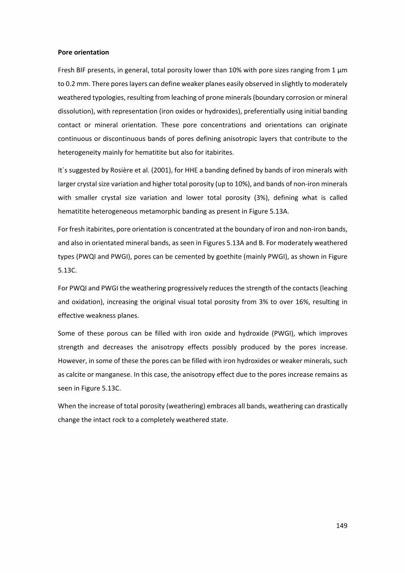
149
Pore orientation
Fresh BIF presents, in general, total porosity lower than 10% with pore sizes ranging from 1 μm
to 0.2 mm. There pores layers can define weaker planes easily observed in slightly to moderately
weathered typologies, resulting from leaching of prone minerals (boundary corrosion or mineral
dissolution), with representation (iron oxides or hydroxides), preferentially using initial banding
contact or mineral orientation. These pore concentrations and orientations can originate
continuous or discontinuous bands of pores defining anisotropic layers that contribute to the
heterogeneity mainly for hematitite but also for itabirites.
It´s suggested by Rosière et al. (2001), for HHE a banding defined by bands of iron minerals with
larger crystal size variation and higher total porosity (up to 10%), and bands of non-iron minerals
with smaller crystal size variation and lower total porosity (3%), defining what is called
hematitite heterogeneous metamorphic banding as present in Figure 5.13A.
For fresh itabirites, pore orientation is concentrated at the boundary of iron and non-iron bands,
and also in orientated mineral bands, as seen in Figures 5.13A and B. For moderately weathered
types (PWQI and PWGI), pores can be cemented by goethite (mainly PWGI), as shown in Figure
5.13C.
For PWQI and PWGI the weathering progressively reduces the strength of the contacts (leaching
and oxidation), increasing the original visual total porosity from 3% to over 16%, resulting in
effective weakness planes.
Some of these porous can be filled with iron oxide and hydroxide (PWGI), which improves
strength and decreases the anisotropy effects possibly produced by the pores increase.
However, in some of these the pores can be filled with iron hydroxides or weaker minerals, such
as calcite or manganese. In this case, the anisotropy effect due to the pores increase remains as
seen in Figure 5.13C.
When the increase of total porosity (weathering) embraces all bands, weathering can drastically
change the intact rock to a completely weathered state.
150
(A) (B)
(C)
36 Figure 5.13 A (left), pore bands in massive HHE. B (centre), FWQI microphotography showing
porosity (delimited in red lines) between quartz (lightly coloured) and hematite
(light grey) contact. C (right) PWGI presenting hematite (white) and quartz (grey)
bands with different crystal sizes at contact (dark); Horta & Costa (2016)
Total porosity seems to be the most important characteristic that defines the anisotropy of the
HHE and very important for others BIF. The overall porosity distribution defines the intact rock
fabric as a response to the banding boundary and orientated elongated mineral fabrics, which
are the aspects that define the different BIF internal textural web ’skeleton ‘, providing weakness
surfaces or bands. These voids are weathering preferential zones that will induce a continued
intact rock strength reduction as weathering increases, inducing effective mineral contact
reduction by leaching and chemical alteration, and ultimately increasing the total porosity.
In some cases when concentrated, this process causes real discontinuities, generating intact rock
interruption (continuum break).
1000 μm 0.5 mm
0.5 mm
151
Furthermore, this research did not evaluate quantitatively the boundary banding, elongated
orientated minerals and total porosity effects. For this reason, it is not possible to define the
most important characteristic that defines the anisotropy index for fresh, slightly, and
moderately weathered BIF.
5.5.3 Anisotropy evaluations of dynamic elastic parameters and petrophysical
properties
This section presents the dynamic elastic parameters, obtained from Vp and Vs wave velocity
propagation tests conducted in different anisotropy angles (βangle) evaluation of fresh and
moderately weathered BIF. These results were used to determine anisotropy effects and elastic
parameter based on empirical correlations and determine the relationship between wave
velocity propagation, dynamic elastic parameters (Young’s modulus and Poisson’s ratio) and
petrophysical properties (bulk density, and total porosity).
Table 5.2 summarises test results for FQI, FDI, FAI, and PWQI/PWGI for each βangle (0°, 45°, and
90°). Basic statistical evaluation is presented in this table for each type: mean, standard deviation
(SD), maximum values (Max), minimum values (Min), and number of tested samples (n).
Considering the inadequate number of total test results for HHE (n = 4) has not been evaluated
in this section. Some results can present bias, due to the reduced number of tests in some
direction, mainly FAI0° (n = 2). Due to the reduced number of available tests, the PWQI and PWGI
were considered as a single group, supported by the similar geological and geomechanical
features.
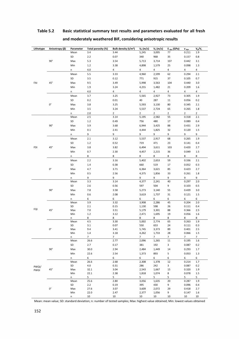
152
9 Table 5.2 Basic statistical summary test results and parameters evaluated for all fresh
and moderately weathered BIF, considering anisotropic results
Lithotype Anisotropy (β) Parameter Total porosity (%) Bulk density (t/m3) VP (m/s) VS (m/s) E dyn (GPa) v dyn Vp/Vs
FAI
90°
Mean 3.4 3.44 5,245 3,005 77 0.211 1.9 SD 2.2 0.07 340 968 35 0.157 0.8 Max 5.3 3.54 5,713 3,714 107 0.442 3.1 Min 1.2 3.38 4,898 1,579 25 0.098 1.3 n 4.0 4 4 4 4 4 4
45°
Mean 5.5 3.33 4,960 2,599 62 0.294 2.1 SD 3.5 0.12 771 915 37 0.105 0.7 Max 9.5 3.49 5,998 3,563 104 0.440 3.0 Min 1.9 3.24 4,255 1,482 21 0.209 1.6 n 4.0 4 4 4 4 4 4
0°
Mean 3.7 3.25 5,565 2,927 73 0.305 1.9 SD 0.2 0.01 40 287 11 0.056 0.2 Max 3.8 3.25 5,593 3,130 80 0.345 2.1 Min 3.5 3.24 5,537 2,724 65 0.265 1.8 n 2.0 2 2 2 2 2 2
FDI
90°
Mean 2.5 3.14 5,195 2,582 55 0.318 2.1 SD 1.2 0.49 756 480 17 0.089 0.4 Max 3.9 3.68 6,944 3,425 88 0.431 2.9 Min 0.1 2.41 4,444 1,825 32 0.120 1.5 n 9 9 9 9 9 9 9
45°
Mean 2.1 3.12 5,537 2,917 68 0.265 1.9 SD 1.2 0.52 719 471 23 0.141 0.4 Max 3.8 3.82 6,494 3,611 103 0.420 2.7 Min 0.7 2.30 4,457 2,215 36 0.049 1.5 n 8 8 8 8 8 8 8
0°
Mean 2.2 3.16 5,402 2,653 59 0.336 2.1 SD 1.4 0.38 660 519 17 0.052 0.3 Max 4.7 3.71 6,364 3,621 85 0.423 2.7 Min 0.5 2.56 4,375 1,856 33 0.261 1.8 n 9 9 9 9 9 9 9
FQI
90°
Mean 3.3 3.14 4,377 2,241 40 0.297 2.0 SD 2.6 0.56 597 504 9 0.103 0.5 Max 7.8 3.58 5,273 3,140 55 0.439 3.0 Min 0.6 2.08 3,619 1,737 31 0.121 1.5 n 6 6 6 6 6 6 6
45°
Mean 3.9 3.32 3,908 2,286 45 0.204 2.0 SD 2.1 0.15 1,130 598 26 0.111 0.4 Max 7.0 3.51 5,179 3,301 88 0.366 2.5 Min 1.2 3.12 2,471 1,695 19 0.056 1.6 n 8 8 8 8 8 8 8
0°
Mean 4.5 3.30 5,002 2,774 65 0.263 1.9 SD 3.1 0.07 550 653 24 0.111 0.3 Max 9.4 3.41 5,745 3,373 89 0.401 2.5 Min 1.4 3.18 4,262 1,733 28 0.066 1.5 n 7 7 7 7 7 7 7
PWQI/ PWGI
90°
Mean 26.6 2.77 2,096 1,265 11 0.195 1.6 SD 2.7 0.17 381 192 3 0.087 0.2 Max 30.0 2.94 2,484 1,449 14 0.293 1.7 Min 22.6 2.54 1,373 893 5 0.053 1.3 n 6 6 6 6 6 6 6
45°
Mean 26.6 2.68 2,308 1,378 12 0.214 1.7 SD 4.0 0.31 286 242 3 0.087 0.2 Max 32.1 3.04 2,543 1,667 15 0.320 1.9 Min 22.1 2.38 1,818 1,074 8 0.078 1.5 n 5 5 5 5 5 5 5
0°
Mean 25.6 2.80 3,056 1,635 20 0.287 1.9 SD 2.2 0.19 395 430 9 0.096 0.4 Max 27.6 3.07 3,609 2,072 29 0.418 2.7 Min 22.0 2.47 2,377 1,056 9 0.147 1.6 n 10 10 10 10 10 10 10
Mean: mean value; SD: standard deviation; n: number of tested samples; Max: highest value obtained; Min: lowest values obtained
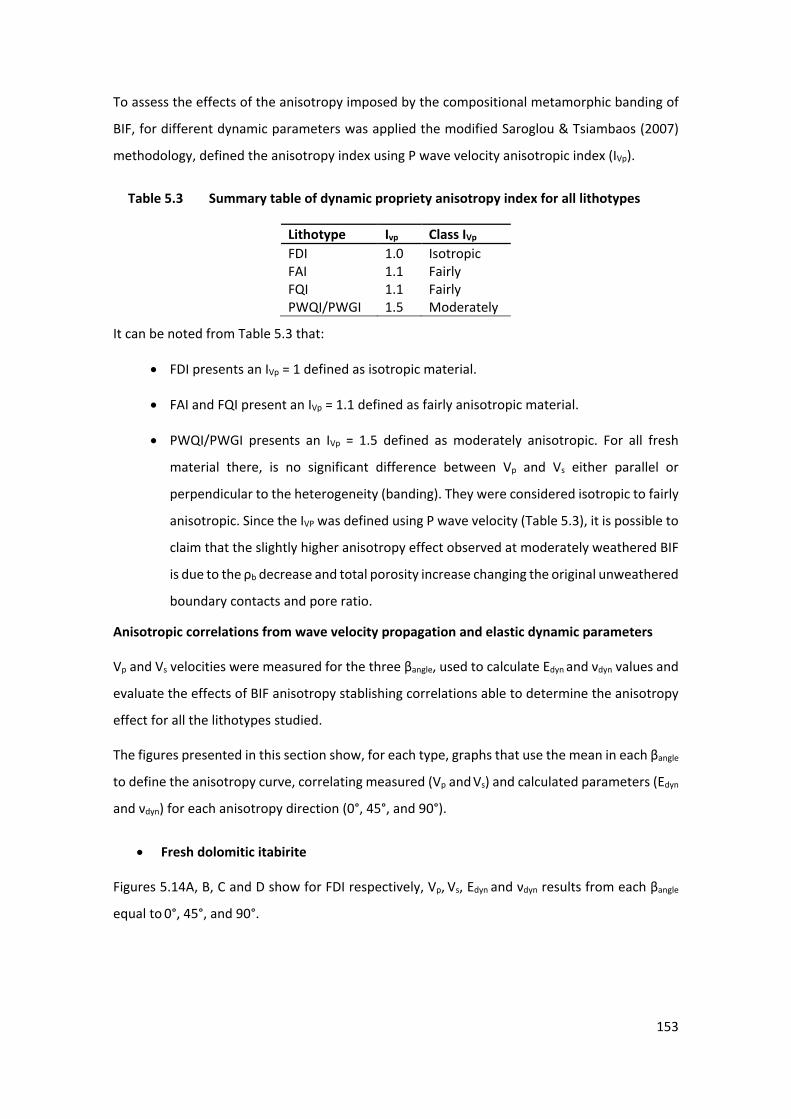
153
To assess the effects of the anisotropy imposed by the compositional metamorphic banding of
BIF, for different dynamic parameters was applied the modified Saroglou & Tsiambaos (2007)
methodology, defined the anisotropy index using P wave velocity anisotropic index (IVp).
10Table 5.3 Summary table of dynamic propriety anisotropy index for all lithotypes
Lithotype Ivp Class IVp FDI 1.0 Isotropic FAI 1.1 Fairly FQI 1.1 Fairly PWQI/PWGI 1.5 Moderately
It can be noted from Table 5.3 that:
• FDI presents an IVp = 1 defined as isotropic material.
• FAI and FQI present an IVp = 1.1 defined as fairly anisotropic material.
• PWQI/PWGI presents an IVp = 1.5 defined as moderately anisotropic. For all fresh
material there, is no significant difference between Vp and Vs either parallel or
perpendicular to the heterogeneity (banding). They were considered isotropic to fairly
anisotropic. Since the IVP was defined using P wave velocity (Table 5.3), it is possible to
claim that the slightly higher anisotropy effect observed at moderately weathered BIF
is due to the ρb decrease and total porosity increase changing the original unweathered
boundary contacts and pore ratio.
Anisotropic correlations from wave velocity propagation and elastic dynamic parameters
Vp and Vs velocities were measured for the three βangle, used to calculate Edyn and νdyn values and
evaluate the effects of BIF anisotropy stablishing correlations able to determine the anisotropy
effect for all the lithotypes studied.
The figures presented in this section show, for each type, graphs that use the mean in each βangle
to define the anisotropy curve, correlating measured (Vp and Vs) and calculated parameters (Edyn
and νdyn) for each anisotropy direction (0°, 45°, and 90°).
• Fresh dolomitic itabirite
Figures 5.14A, B, C and D show for FDI respectively, Vp, Vs, Edyn and νdyn results from each βangle
equal to 0°, 45°, and 90°.
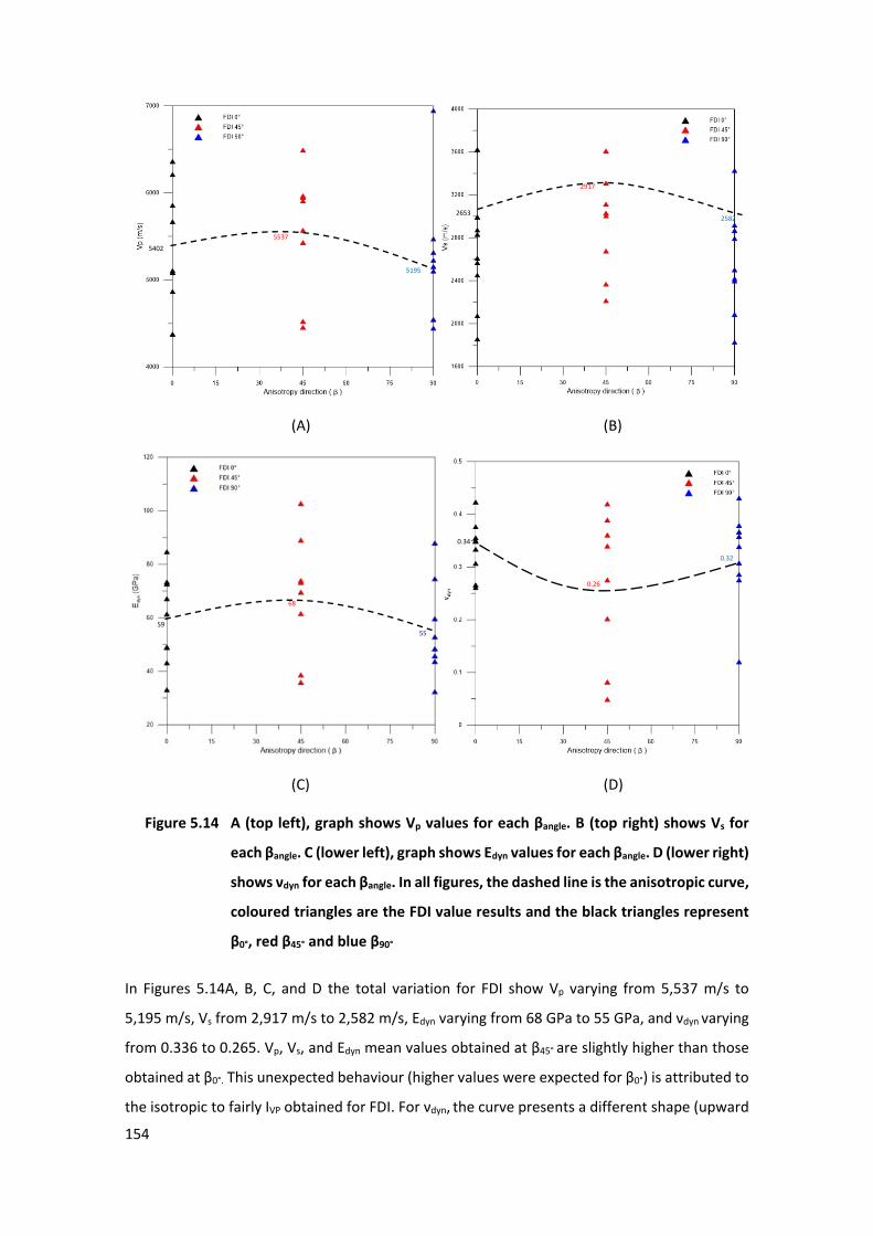
154
(A) (B)
(C) (D)
37 Figure 5.14 A (top left), graph shows Vp values for each βangle. B (top right) shows Vs for
each βangle. C (lower left), graph shows Edyn values for each βangle. D (lower right)
shows νdyn for each βangle. In all figures, the dashed line is the anisotropic curve,
coloured triangles are the FDI value results and the black triangles represent
β0°, red β45° and blue β90°
In Figures 5.14A, B, C, and D the total variation for FDI show Vp varying from 5,537 m/s to
5,195 m/s, Vs from 2,917 m/s to 2,582 m/s, Edyn varying from 68 GPa to 55 GPa, and νdyn varying
from 0.336 to 0.265. Vp, Vs, and Edyn mean values obtained at β45° are slightly higher than those
obtained at β0°. This unexpected behaviour (higher values were expected for β0°) is attributed to
the isotropic to fairly IVP obtained for FDI. For νdyn, the curve presents a different shape (upward
5195
5537 5402
2582
2917
2653
59 55
68
0.32
0.34
0.26
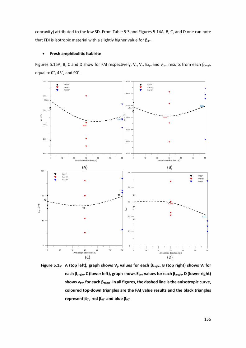
155
concavity) attributed to the low SD. From Table 5.3 and Figures 5.14A, B, C, and D one can note
that FDI is isotropic material with a slightly higher value for β45°.
• Fresh amphibolitic Itabirite
Figures 5.15A, B, C and D show for FAI respectively, Vp, Vs, Edyn and νdyn results from each βangle
equal to 0°, 45°, and 90°.
(A) (B)
(C) (D)
38 Figure 5.15 A (top left), graph shows Vp values for each βangle. B (top right) shows Vs for
each βangle. C (lower left), graph shows Edyn values for each βangle. D (lower right)
shows νdyn for each βangle. In all figures, the dashed line is the anisotropic curve,
coloured top-down triangles are the FAI value results and the black triangles
represent β0°, red β45° and blue β90°
5245
4960
5566
3005
2599
2927
77
62
73 0.294
0.211
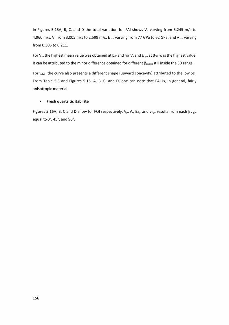
156
In Figures 5.15A, B, C, and D the total variation for FAI shows Vp varying from 5,245 m/s to
4,960 m/s, Vs from 3,005 m/s to 2,599 m/s, Edyn varying from 77 GPa to 62 GPa, and νdyn varying
from 0.305 to 0.211.
For Vp, the highest mean value was obtained at β0° and for Vs and Edyn at β90° was the highest value.
It can be attributed to the minor difference obtained for different βangles still inside the SD range.
For νdyn, the curve also presents a different shape (upward concavity) attributed to the low SD.
From Table 5.3 and Figures 5.15. A, B, C, and D, one can note that FAI is, in general, fairly
anisotropic material.
• Fresh quartzitic itabirite
Figures 5.16A, B, C and D show for FQI respectively, Vp, Vs, Edyn and νdyn results from each βangle
equal to 0°, 45°, and 90°.
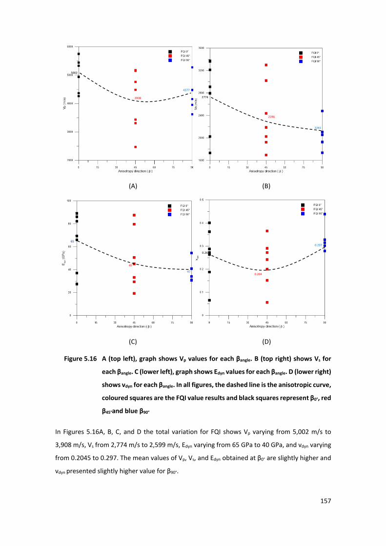
157
(A) (B)
(C) (D)
39 Figure 5.16 A (top left), graph shows Vp values for each βangle. B (top right) shows Vs for
each βangle. C (lower left), graph shows Edyn values for each βangle. D (lower right)
shows νdyn for each βangle. In all figures, the dashed line is the anisotropic curve,
coloured squares are the FQI value results and black squares represent β0°, red
β45°and blue β90°
In Figures 5.16A, B, C, and D the total variation for FQI shows Vp varying from 5,002 m/s to
3,908 m/s, Vs from 2,774 m/s to 2,599 m/s, Edyn varying from 65 GPa to 40 GPa, and νdyn varying
from 0.2045 to 0.297. The mean values of Vp, Vs, and Edyn obtained at β0° are slightly higher and
νdyn presented slightly higher value for β90°.
4377
3908
5002
2241
2286
2774
45
65
40
0.297
0.26
0.204
158
From Table 5.3 and Figures 5.16 A, B, C, and D, one can note that FQI is, in general, fairly
anisotropic material.
Moderately weathered goethitic and quartzitic itabirite
Figures 5.17A, B, C and D show for PWQI and PWGI respectively, Vp, Vs, Edyn and νdyn results from
each βangle equal to 0°, 45°, and 90°.
(A) (B)
(C) (D)
40 Figure 5.17 A (top left), graph shows Vp values for each βangle. B (top right) shows Vs for
each βangle. C (lower left), graph shows Edyn values for each βangle. D (lower right)
shows νdyn for each βangle. In all figures, the dashed line is the anisotropic curve,
coloured crosses are the PWQI/PWGI value results and the black crosses
represent β0°, red β45° and blue β90°
2096 2308
3056
1378
1265
1635
12 11
0.2 0.21
0.29
159
In Figures 5.17A, B, C, and D the total variation for PWQI/PWGI show Vp varying from 3,056 m/s
to 2,069 m/s, Vs from 1,635 m/s to 1,265 m/s, Edyn varying from 20 GPa to 11 GPa, and νdyn
varying from 0.287 to 0.195.
Vp, Vs, and Edyn, and νdyn mean values obtained at β0° are higher and is considered as an expected
behaviour for moderately anisotropic materials even presenting IVP from fairly anisotropic for
Poisson’s ratio.
From Table 5.3 and Figures 5.17A, B, C, and D is possible to note that PWQI/PWGI is moderately
anisotropic material. Showing a clear weathering effect in the ancient fresh rocks behaviour.
5.5.4 Isotropic evaluations of dynamic elastic parameters and petrophysical
properties
Due to the isotropic to fairly IVP for all BIF described in Section 5.5.3, in this section, the
anisotropy was not considered even though it can influence the results and interpretation.
This section presents the dynamic elastic parameters obtained from Vp and Vs velocity
propagation tests not considering the different anisotropy angles (βangle) and evaluating all types
of fresh to moderately weathered BIF as a single group. These results were used to identify
empirical correlations and determine the relationship between wave velocity propagation,
dynamic elastic parameters (Edyn and νdyn) and petrophysical properties (ρb) considering the BIF
as an isotropic material.
Table 5.4 summarises all test results for fresh types and moderately weathered types presenting
the basic statistical evaluation for each type, the mean, standard deviation (SD), maximum
values (Max), minimum values (Min), upper and lower inner fence, covariance (CV), margin of
error, values of the first and third quartiles (1 Qt and 3 Qt), and number of tested samples (n).
Considering the low number of test results, PWQI and PWGI were grouped, also considering the
similarity presented in previous sections. For the same reason, HHE has no statistical support
and some parameters were not presented.
Some results can present bias due to the low number of tests. This affects mainly the HHE tests
with a total of four tests. Even with low test numbers for HHE the anisotropic index obtained
was IVp = 1.1 (fairly anisotropic).
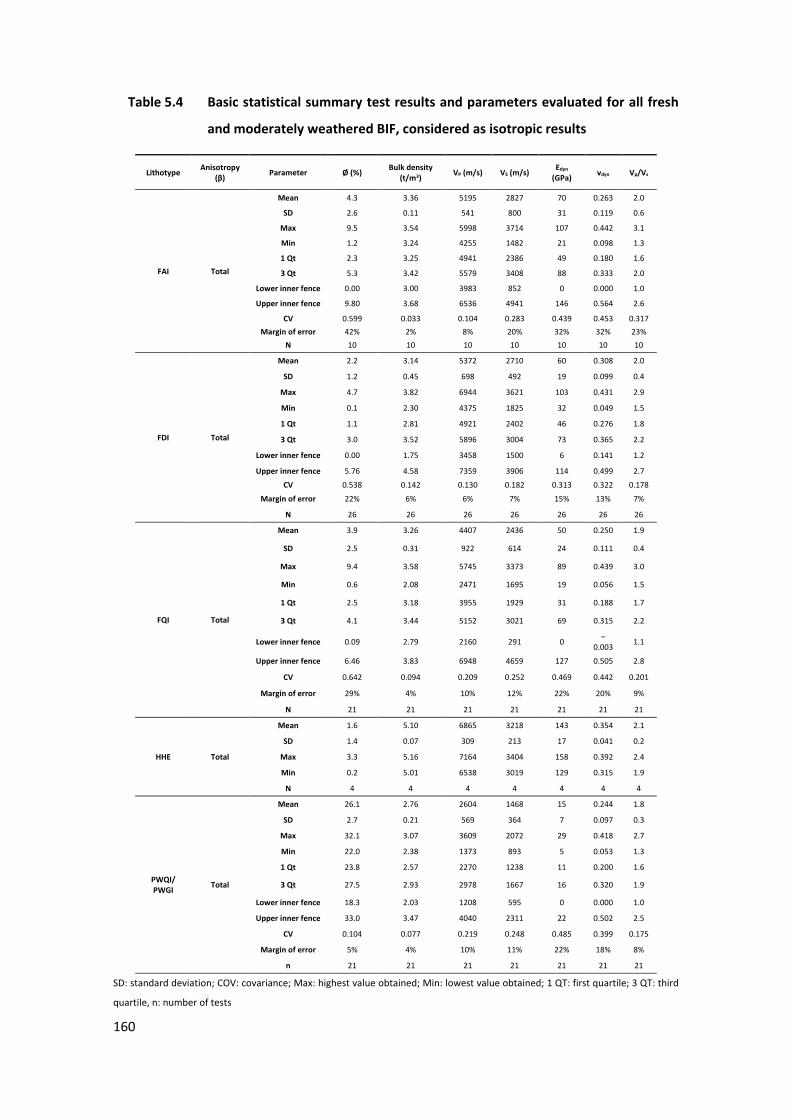
160
11Table 5.4 Basic statistical summary test results and parameters evaluated for all fresh
and moderately weathered BIF, considered as isotropic results
Lithotype Anisotropy (β) Parameter Ø (%) Bulk density
(t/m3) VP (m/s) VS (m/s) Edyn (GPa) vdyn Vp/Vs
FAI Total
Mean 4.3 3.36 5195 2827 70 0.263 2.0
SD 2.6 0.11 541 800 31 0.119 0.6
Max 9.5 3.54 5998 3714 107 0.442 3.1
Min 1.2 3.24 4255 1482 21 0.098 1.3
1 Qt 2.3 3.25 4941 2386 49 0.180 1.6
3 Qt 5.3 3.42 5579 3408 88 0.333 2.0
Lower inner fence 0.00 3.00 3983 852 0 0.000 1.0
Upper inner fence 9.80 3.68 6536 4941 146 0.564 2.6
CV 0.599 0.033 0.104 0.283 0.439 0.453 0.317 Margin of error 42% 2% 8% 20% 32% 32% 23%
N 10 10 10 10 10 10 10
FDI Total
Mean 2.2 3.14 5372 2710 60 0.308 2.0
SD 1.2 0.45 698 492 19 0.099 0.4
Max 4.7 3.82 6944 3621 103 0.431 2.9
Min 0.1 2.30 4375 1825 32 0.049 1.5
1 Qt 1.1 2.81 4921 2402 46 0.276 1.8
3 Qt 3.0 3.52 5896 3004 73 0.365 2.2
Lower inner fence 0.00 1.75 3458 1500 6 0.141 1.2
Upper inner fence 5.76 4.58 7359 3906 114 0.499 2.7
CV 0.538 0.142 0.130 0.182 0.313 0.322 0.178
Margin of error 22% 6% 6% 7% 15% 13% 7%
N 26 26 26 26 26 26 26
FQI Total
Mean 3.9 3.26 4407 2436 50 0.250 1.9
SD 2.5 0.31 922 614 24 0.111 0.4
Max 9.4 3.58 5745 3373 89 0.439 3.0
Min 0.6 2.08 2471 1695 19 0.056 1.5
1 Qt 2.5 3.18 3955 1929 31 0.188 1.7
3 Qt 4.1 3.44 5152 3021 69 0.315 2.2
Lower inner fence 0.09 2.79 2160 291 0 –0.003 1.1
Upper inner fence 6.46 3.83 6948 4659 127 0.505 2.8
CV 0.642 0.094 0.209 0.252 0.469 0.442 0.201
Margin of error 29% 4% 10% 12% 22% 20% 9%
N 21 21 21 21 21 21 21
HHE Total
Mean 1.6 5.10 6865 3218 143 0.354 2.1
SD 1.4 0.07 309 213 17 0.041 0.2
Max 3.3 5.16 7164 3404 158 0.392 2.4
Min 0.2 5.01 6538 3019 129 0.315 1.9
N 4 4 4 4 4 4 4
PWQI/ PWGI Total
Mean 26.1 2.76 2604 1468 15 0.244 1.8
SD 2.7 0.21 569 364 7 0.097 0.3
Max 32.1 3.07 3609 2072 29 0.418 2.7
Min 22.0 2.38 1373 893 5 0.053 1.3
1 Qt 23.8 2.57 2270 1238 11 0.200 1.6
3 Qt 27.5 2.93 2978 1667 16 0.320 1.9
Lower inner fence 18.3 2.03 1208 595 0 0.000 1.0
Upper inner fence 33.0 3.47 4040 2311 22 0.502 2.5
CV 0.104 0.077 0.219 0.248 0.485 0.399 0.175
Margin of error 5% 4% 10% 11% 22% 18% 8%
n 21 21 21 21 21 21 21
SD: standard deviation; COV: covariance; Max: highest value obtained; Min: lowest value obtained; 1 QT: first quartile; 3 QT: third
quartile, n: number of tests
161
From Table 5.4 results is possible to note that:
• Total porosity
High SD for fresh lithotypes.
Lower relative values obtained for HHE = 1.6% (±1.4) and FDI = 2.2% (±1.2); moderate
for FQI = 3.9% (±2.5) and FAI = 4.3% (±2.6); and higher values for PWQI/PWGI = 26.1%
(±2.7).
Comparing visual total porosity (Øb), from thin sections with total porosity (Ø), from
poropermiameter tests, is possible to note that for FAI (Øb = 5% and Ø = 4.3 ± 2.6), for
FDI (Øb = 6% and Ø = 2.2 ± 1.2), for FQI (Øb = 12% and Ø = 3.4 ± 2.5), for HHE (Øb = 6%
and Ø = 1.6 ± 1.4) and for PWQI/PWGI (Øb = 13% and Ø = 26 ± 2.7). Reaching a proper
correlating for FAI but in general, Øb overestimate the total porosity for FDI, FQI and
HHE, and underestimate for PWQI/PWGI.
• Bulk density
Low SD for all tested lithotypes.
Lower relative values obtained for PWQI/PWGI= 2.76 (±0.21) t/m3; moderate for FAI=
3.36 (±0.11) t/m3, FQI= 3.26 (±0.31) t/m3 and FDI= 3.14 (±0.45) t/m3; and higher values
for HHE = 5.10 (±0.07) t/m3.
• P wave velocity
Low SD for all tested lithotypes.
Low relative values for PWQI/PWGI = 2,604 (±569) m/s; moderate for
FQI = 4,407 (±922) m/s; high for FAI = 5,195 (±541) m/s and FDI = 5,372 (±698) m/s;
and very high for HHE = 6,865 (±309) m/s.
• S wave velocity
Low SD for all tested lithotypes.
Lower relative values for PWQI/PWGI = 1,468 (±364) m/s; moderate for FQI =
2,436 (±614) m/s; high for FAI = 2,927 (±800) m/s and FDI = 2,710 (±492) m/s; and very
high for HHE = 3,218 (±213) m/s.
• Dynamic elastic modulus
High SD for all tested lithotypes.
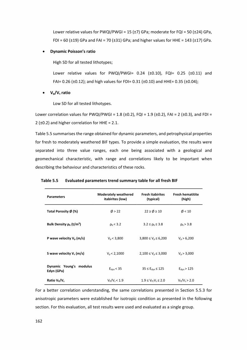
162
Lower relative values for PWQI/PWGI = 15 (±7) GPa; moderate for FQI = 50 (±24) GPa,
FDI = 60 (±19) GPa and FAI = 70 (±31) GPa; and higher values for HHE = 143 (±17) GPa.
• Dynamic Poisson’s ratio
High SD for all tested lithotypes;
Lower relative values for PWQI/PWGI= 0.24 (±0.10), FQI= 0.25 (±0.11) and
FAI= 0.26 (±0.12); and high values for FDI= 0.31 (±0.10) and HHE= 0.35 (±0.04);
• Vp/Vs ratio
Low SD for all tested lithotypes.
Lower correlation values for PWQI/PWGI = 1.8 (±0.2), FQI = 1.9 (±0.2), FAI = 2 (±0.3), and FDI =
2 (±0.2) and higher correlation for HHE = 2.1.
Table 5.5 summarises the range obtained for dynamic parameters, and petrophysical properties
for fresh to moderately weathered BIF types. To provide a simple evaluation, the results were
separated into three value ranges, each one being associated with a geological and
geomechanical characteristic, with range and correlations likely to be important when
describing the behaviour and characteristics of these rocks.
12 Table 5.5 Evaluated parameters trend summary table for all fresh BIF
Parameters Moderately weathered itabirites (low)
Fresh itabirites (typical)
Fresh hematitite (high)
Total Porosity Ø (%) Ø > 22 22 ≥ Ø ≥ 10 Ø < 10
Bulk Density ρb (t/m3) ρb < 3.2 3.2 ≤ ρb ≤ 3.8 ρb > 3.8
P wave velocity Vp (m/s) Vp < 3,800 3,800 ≤ Vp ≤ 6,200 Vp > 6,200
S wave velocity Vs (m/s) Vp < 2,1000 2,100 ≤ Vp ≤ 3,000 Vp > 3,000
Dynamic Young's modulus Edyn (GPa) Edyn < 35 35 ≤ Edyn ≤ 125 Edyn > 125
Ratio VP/Vs VP/Vs < 1.9 1.9 ≤ VP/Vs ≤ 2.0 VP/Vs > 2.0
For a better correlation understanding, the same correlations presented in Section 5.5.3 for
anisotropic parameters were established for isotropic condition as presented in the following
section. For this evaluation, all test results were used and evaluated as a single group.
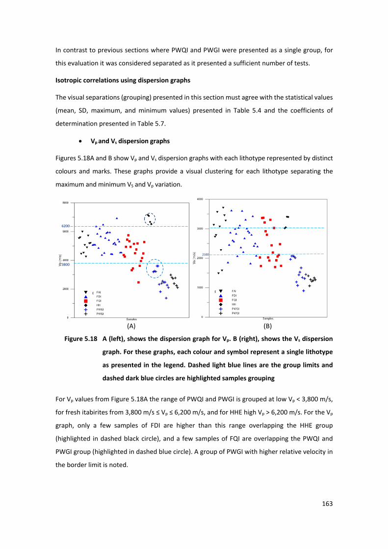
163
In contrast to previous sections where PWQI and PWGI were presented as a single group, for
this evaluation it was considered separated as it presented a sufficient number of tests.
Isotropic correlations using dispersion graphs
The visual separations (grouping) presented in this section must agree with the statistical values
(mean, SD, maximum, and minimum values) presented in Table 5.4 and the coefficients of
determination presented in Table 5.7.
• Vp and Vs dispersion graphs
Figures 5.18A and B show Vp and Vs dispersion graphs with each lithotype represented by distinct
colours and marks. These graphs provide a visual clustering for each lithotype separating the
maximum and minimum VS and Vp variation.
(A) (B)
41 Figure 5.18 A (left), shows the dispersion graph for Vp. B (right), shows the Vs dispersion
graph. For these graphs, each colour and symbol represent a single lithotype
as presented in the legend. Dashed light blue lines are the group limits and
dashed dark blue circles are highlighted samples grouping
For Vp values from Figure 5.18A the range of PWQI and PWGI is grouped at low Vp < 3,800 m/s,
for fresh itabirites from 3,800 m/s ≤ Vp ≤ 6,200 m/s, and for HHE high Vp > 6,200 m/s. For the Vp
graph, only a few samples of FDI are higher than this range overlapping the HHE group
(highlighted in dashed black circle), and a few samples of FQI are overlapping the PWQI and
PWGI group (highlighted in dashed blue circle). A group of PWGI with higher relative velocity in
the border limit is noted.
3800
6200
2100
E E
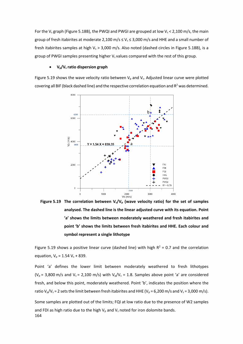
164
For the Vs graph (Figure 5.18B), the PWQI and PWGI are grouped at low Vs < 2,100 m/s, the main
group of fresh itabirites at moderate 2,100 m/s ≤ Vs ≤ 3,000 m/s and HHE and a small number of
fresh itabirites samples at high Vs > 3,000 m/s. Also noted (dashed circles in Figure 5.18B), is a
group of PWGI samples presenting higher Vs values compared with the rest of this group.
• Vp/Vs ratio dispersion graph
Figure 5.19 shows the wave velocity ratio between Vp and Vs. Adjusted linear curve were plotted
covering all BIF (black dashed line) and the respective correlation equation and R2 was determined.
42 Figure 5.19 The correlation between Vs/Vp (wave velocity ratio) for the set of samples
analysed. The dashed line is the linear adjusted curve with its equation. Point
’a’ shows the limits between moderately weathered and fresh itabirites and
point ‘b’ shows the limits between fresh itabirites and HHE. Each colour and
symbol represent a single lithotype
Figure 5.19 shows a positive linear curve (dashed line) with high R2 = 0.7 and the correlation
equation, Vp = 1.54 Vs + 839.
Point ‘a’ defines the lower limit between moderately weathered to fresh lithotypes
(Vp = 3,800 m/s and Vs = 2,100 m/s) with Vp/Vs = 1.8. Samples above point ‘a’ are considered
fresh, and below this point, moderately weathered. Point ’b’, indicates the position where the
ratio Vp/Vs = 2 sets the limit between fresh itabirites and HHE (Vp = 6,200 m/s and Vs = 3,000 m/s).
Some samples are plotted out of the limits; FQI at low ratio due to the presence of W2 samples
and FDI as high ratio due to the high Vp and Vs noted for iron dolomite bands.
a
b
3800
6200
2100
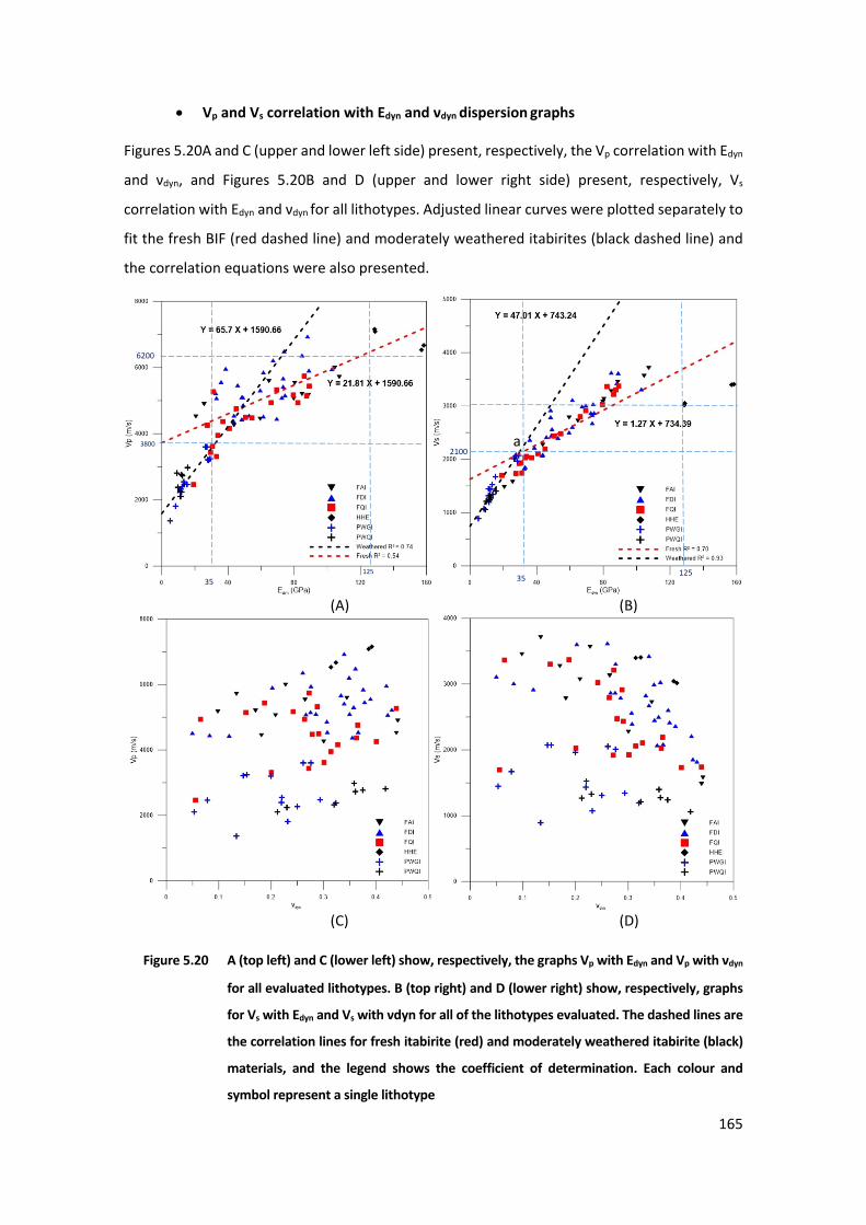
165
• Vp and Vs correlation with Edyn and νdyn dispersion graphs
Figures 5.20A and C (upper and lower left side) present, respectively, the Vp correlation with Edyn
and νdyn, and Figures 5.20B and D (upper and lower right side) present, respectively, Vs
correlation with Edyn and νdyn for all lithotypes. Adjusted linear curves were plotted separately to
fit the fresh BIF (red dashed line) and moderately weathered itabirites (black dashed line) and
the correlation equations were also presented.
(A) (B)
(C) (D)
43 Figure 5.20 A (top left) and C (lower left) show, respectively, the graphs Vp with Edyn and Vp with νdyn
for all evaluated lithotypes. B (top right) and D (lower right) show, respectively, graphs
for Vs with Edyn and Vs with νdyn for all of the lithotypes evaluated. The dashed lines are
the correlation lines for fresh itabirite (red) and moderately weathered itabirite (black)
materials, and the legend shows the coefficient of determination. Each colour and
symbol represent a single lithotype
a
6200
3800
35 125
35 125
2100
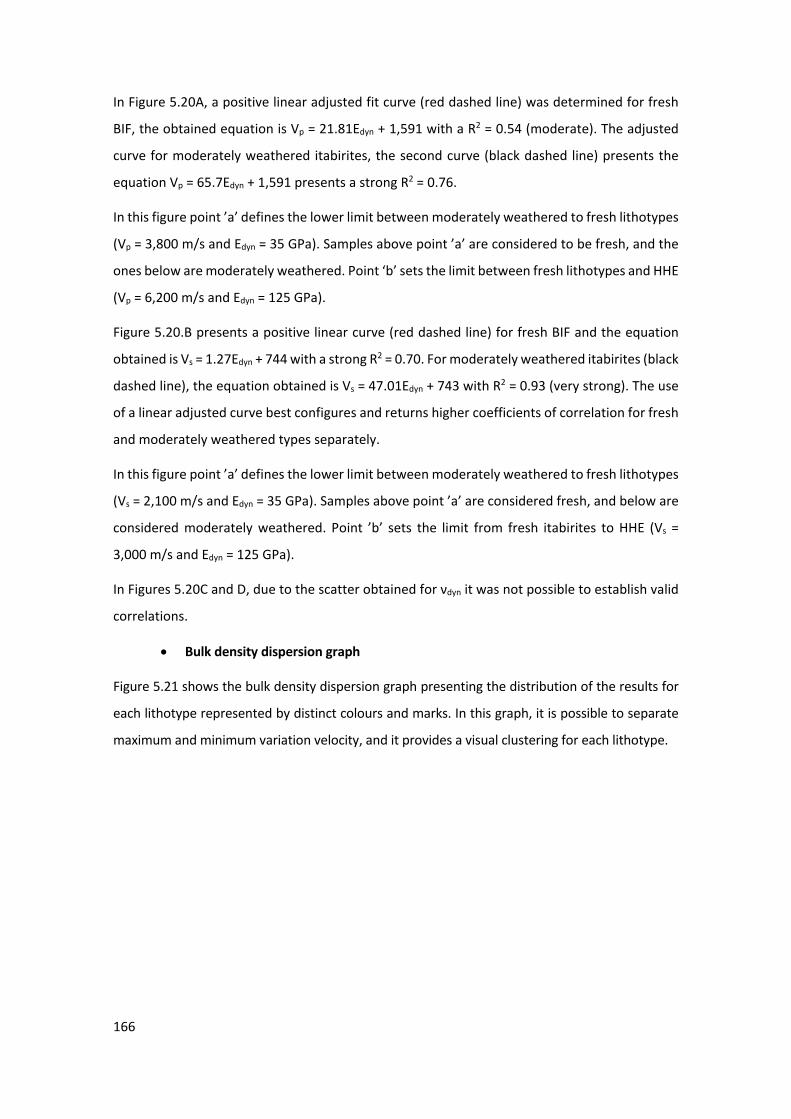
166
In Figure 5.20A, a positive linear adjusted fit curve (red dashed line) was determined for fresh
BIF, the obtained equation is Vp = 21.81Edyn + 1,591 with a R2 = 0.54 (moderate). The adjusted
curve for moderately weathered itabirites, the second curve (black dashed line) presents the
equation Vp = 65.7Edyn + 1,591 presents a strong R2 = 0.76.
In this figure point ’a’ defines the lower limit between moderately weathered to fresh lithotypes
(Vp = 3,800 m/s and Edyn = 35 GPa). Samples above point ’a’ are considered to be fresh, and the
ones below are moderately weathered. Point ‘b’ sets the limit between fresh lithotypes and HHE
(Vp = 6,200 m/s and Edyn = 125 GPa).
Figure 5.20.B presents a positive linear curve (red dashed line) for fresh BIF and the equation
obtained is Vs = 1.27Edyn + 744 with a strong R2 = 0.70. For moderately weathered itabirites (black
dashed line), the equation obtained is Vs = 47.01Edyn + 743 with R2 = 0.93 (very strong). The use
of a linear adjusted curve best configures and returns higher coefficients of correlation for fresh
and moderately weathered types separately.
In this figure point ’a’ defines the lower limit between moderately weathered to fresh lithotypes
(Vs = 2,100 m/s and Edyn = 35 GPa). Samples above point ’a’ are considered fresh, and below are
considered moderately weathered. Point ’b’ sets the limit from fresh itabirites to HHE (Vs =
3,000 m/s and Edyn = 125 GPa).
In Figures 5.20C and D, due to the scatter obtained for νdyn it was not possible to establish valid
correlations.
• Bulk density dispersion graph
Figure 5.21 shows the bulk density dispersion graph presenting the distribution of the results for
each lithotype represented by distinct colours and marks. In this graph, it is possible to separate
maximum and minimum variation velocity, and it provides a visual clustering for each lithotype.
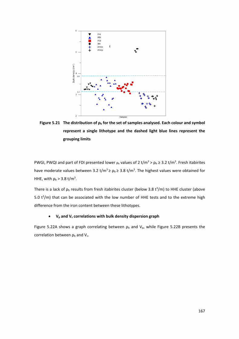
167
44 Figure 5.21 The distribution of ρb for the set of samples analysed. Each colour and symbol
represent a single lithotype and the dashed light blue lines represent the
grouping limits
PWGI, PWQI and part of FDI presented lower ρb values of 2 t/m3 > ρb ≥ 3.2 t/m3. Fresh itabirites
have moderate values between 3.2 t/m3 ≥ ρb ≥ 3.8 t/m3. The highest values were obtained for
HHE, with ρb > 3.8 t/m3.
There is a lack of ρb results from fresh itabirites cluster (below 3.8 t3/m) to HHE cluster (above
5.0 t3/m) that can be associated with the low number of HHE tests and to the extreme high
difference from the iron content between these lithotypes.
• Vp and Vs correlations with bulk density dispersion graph
Figure 5.22A shows a graph correlating between ρb and Vp, while Figure 5.22B presents the
correlation between ρb and Vs.
E
3.2
3.8
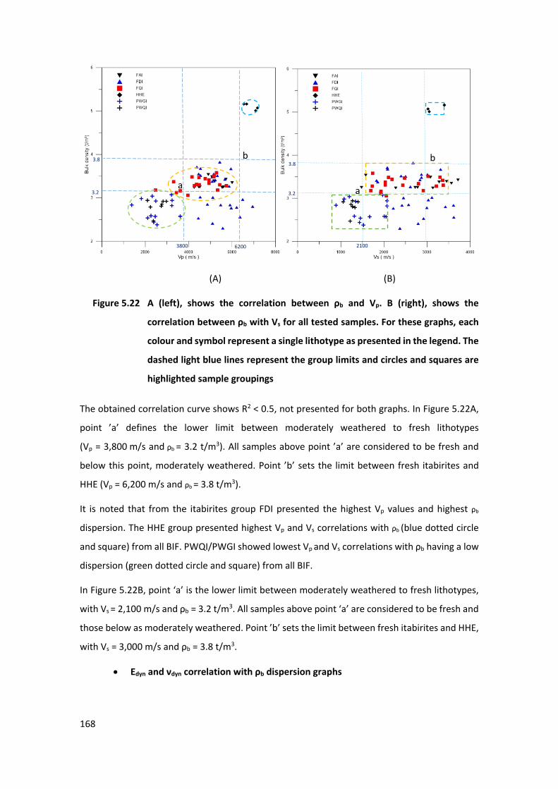
168
(A) (B)
45 Figure 5.22 A (left), shows the correlation between ρb and Vp. B (right), shows the
correlation between ρb with Vs for all tested samples. For these graphs, each
colour and symbol represent a single lithotype as presented in the legend. The
dashed light blue lines represent the group limits and circles and squares are
highlighted sample groupings
The obtained correlation curve shows R2 < 0.5, not presented for both graphs. In Figure 5.22A,
point ’a’ defines the lower limit between moderately weathered to fresh lithotypes
(Vp = 3,800 m/s and ρb = 3.2 t/m3). All samples above point ’a’ are considered to be fresh and
below this point, moderately weathered. Point ’b’ sets the limit between fresh itabirites and
HHE (Vp = 6,200 m/s and ρb = 3.8 t/m3).
It is noted that from the itabirites group FDI presented the highest Vp values and highest ρb
dispersion. The HHE group presented highest Vp and Vs correlations with ρb (blue dotted circle
and square) from all BIF. PWQI/PWGI showed lowest Vp and Vs correlations with ρb having a low
dispersion (green dotted circle and square) from all BIF.
In Figure 5.22B, point ‘a’ is the lower limit between moderately weathered to fresh lithotypes,
with Vs = 2,100 m/s and ρb = 3.2 t/m3. All samples above point ‘a’ are considered to be fresh and
those below as moderately weathered. Point ’b’ sets the limit between fresh itabirites and HHE,
with Vs = 3,000 m/s and ρb = 3.8 t/m3.
• Edyn and νdyn correlation with ρb dispersion graphs
b
a
b
a
3.8 3.8
3.2 3.2
3800 6200 2100
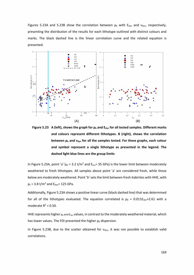
169
Figures 5.23A and 5.23B show the correlation between ρb with Edyn and νdyn, respectively,
presenting the distribution of the results for each lithotype outlined with distinct colours and
marks. The black dashed line is the linear correlation curve and the related equation is
presented.
(A) (B)
46 Figure 5.23 A (left), shows the graph for ρb and Edyn for all tested samples. Different marks
and colours represent different lithotypes. B (right), shows the correlation
between ρb and νdyn for all the samples tested. For these graphs, each colour
and symbol represent a single lithotype as presented in the legend. The
dashed light blue lines are the group limits
In Figure 5.23A, point ’a’ (ρb = 3.2 t/m3 and Edyn= 35 GPa) is the lower limit between moderately
weathered to fresh lithotypes. All samples above point ’a’ are considered fresh, while those
below are moderately weathered. Point ’b’ sets the limit between fresh itabirites with HHE, with
ρb = 3.8 t/m3 and Edyn= 125 GPa.
Additionally, Figure 5.23A shows a positive linear curve (black dashed line) that was determined
for all of the lithotypes evaluated. The equation correlated is ρb = 0.011Edyn+2.61 with a
moderate R2 = 0.50.
HHE represents higher ρb and Edyn values, in contrast to the moderately weathered material, which
has lower values. The FDI presented the higher ρb dispersion.
In Figure 5.23B, due to the scatter obtained for νdyn, it was not possible to establish valid
correlations.
a
b 3.8
3.2
35 125
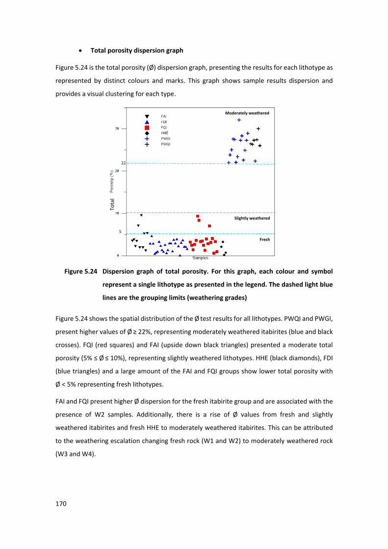
170
• Total porosity dispersion graph
Figure 5.24 is the total porosity (Ø) dispersion graph, presenting the results for each lithotype as
represented by distinct colours and marks. This graph shows sample results dispersion and
provides a visual clustering for each type.
47 Figure 5.24 Dispersion graph of total porosity. For this graph, each colour and symbol
represent a single lithotype as presented in the legend. The dashed light blue
lines are the grouping limits (weathering grades)
Figure 5.24 shows the spatial distribution of the Ø test results for all lithotypes. PWQI and PWGI,
present higher values of Ø ≥ 22%, representing moderately weathered itabirites (blue and black
crosses). FQI (red squares) and FAI (upside down black triangles) presented a moderate total
porosity (5% ≤ Ø ≤ 10%), representing slightly weathered lithotypes. HHE (black diamonds), FDI
(blue triangles) and a large amount of the FAI and FQI groups show lower total porosity with
Ø < 5% representing fresh lithotypes.
FAI and FQI present higher Ø dispersion for the fresh itabirite group and are associated with the
presence of W2 samples. Additionally, there is a rise of Ø values from fresh and slightly
weathered itabirites and fresh HHE to moderately weathered itabirites. This can be attributed
to the weathering escalation changing fresh rock (W1 and W2) to moderately weathered rock
(W3 and W4).
E
Fresh
Slightly weathered
Moderately weathered
5
22
Tota
l
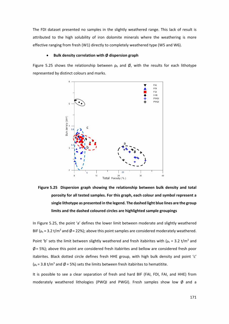
171
The FDI dataset presented no samples in the slightly weathered range. This lack of result is
attributed to the high solubility of iron dolomite minerals where the weathering is more
effective ranging from fresh (W1) directly to completely weathered type (W5 and W6).
• Bulk density correlation with Ø dispersion graph
Figure 5.25 shows the relationship between ρb and Ø, with the results for each lithotype
represented by distinct colours and marks.
48 Figure 5.25 Dispersion graph showing the relationship between bulk density and total
porosity for all tested samples. For this graph, each colour and symbol represent a
single lithotype as presented in the legend. The dashed light blue lines are the group
limits and the dashed coloured circles are highlighted sample groupings
In Figure 5.25, the point ‘a’ defines the lower limit between moderate and slightly weathered
BIF (ρb = 3.2 t/m3 and Ø = 22%); above this point samples are considered moderately weathered.
Point ‘b’ sets the limit between slightly weathered and fresh itabirites with (ρb = 3.2 t/m3 and
Ø = 5%); above this point are considered fresh itabirites and bellow are considered fresh poor
itabirites. Black dotted circle defines fresh HHE group, with high bulk density and point ‘c’
(ρb = 3.8 t/m3 and Ø = 5%) sets the limits between fresh itabirites to hematitite.
It is possible to see a clear separation of fresh and hard BIF (FAI, FDI, FAI, and HHE) from
moderately weathered lithologies (PWQI and PWGI). Fresh samples show low Ø and a
5 22
3.2
3.8
a b
c
Total
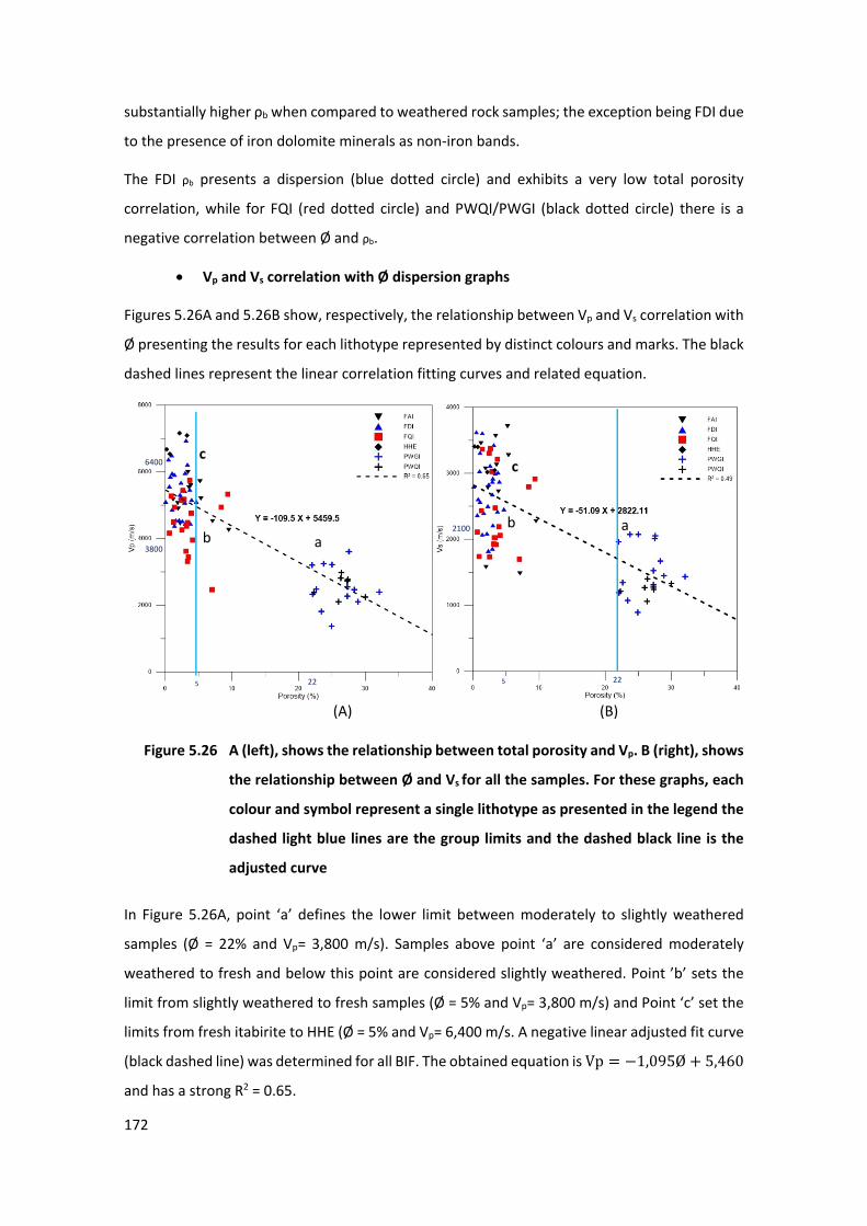
172
substantially higher ρb when compared to weathered rock samples; the exception being FDI due
to the presence of iron dolomite minerals as non-iron bands.
The FDI ρb presents a dispersion (blue dotted circle) and exhibits a very low total porosity
correlation, while for FQI (red dotted circle) and PWQI/PWGI (black dotted circle) there is a
negative correlation between Ø and ρb.
• Vp and Vs correlation with Ø dispersion graphs
Figures 5.26A and 5.26B show, respectively, the relationship between Vp and Vs correlation with
Ø presenting the results for each lithotype represented by distinct colours and marks. The black
dashed lines represent the linear correlation fitting curves and related equation.
(A) (B)
49 Figure 5.26 A (left), shows the relationship between total porosity and Vp. B (right), shows
the relationship between Ø and Vs for all the samples. For these graphs, each
colour and symbol represent a single lithotype as presented in the legend the
dashed light blue lines are the group limits and the dashed black line is the
adjusted curve
In Figure 5.26A, point ‘a’ defines the lower limit between moderately to slightly weathered
samples (Ø = 22% and Vp= 3,800 m/s). Samples above point ‘a’ are considered moderately
weathered to fresh and below this point are considered slightly weathered. Point ’b’ sets the
limit from slightly weathered to fresh samples (Ø = 5% and Vp= 3,800 m/s) and Point ‘c’ set the
limits from fresh itabirite to HHE (Ø = 5% and Vp= 6,400 m/s. A negative linear adjusted fit curve
(black dashed line) was determined for all BIF. The obtained equation is Vp = −1,095Ø + 5,460
and has a strong R2 = 0.65.
b b
a a
3800
6400
2100
5 22 5 22
c c
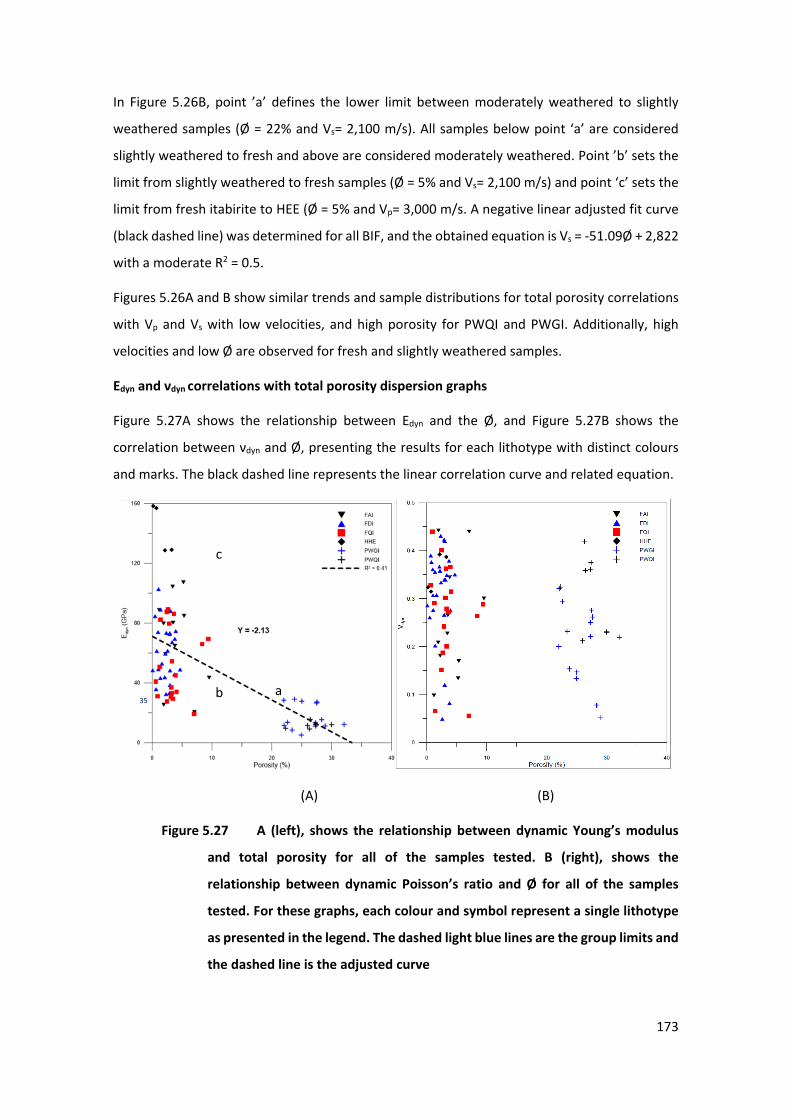
173
In Figure 5.26B, point ’a’ defines the lower limit between moderately weathered to slightly
weathered samples (Ø = 22% and Vs= 2,100 m/s). All samples below point ‘a’ are considered
slightly weathered to fresh and above are considered moderately weathered. Point ’b’ sets the
limit from slightly weathered to fresh samples (Ø = 5% and Vs= 2,100 m/s) and point ‘c’ sets the
limit from fresh itabirite to HEE (Ø = 5% and Vp= 3,000 m/s. A negative linear adjusted fit curve
(black dashed line) was determined for all BIF, and the obtained equation is Vs = -51.09Ø + 2,822
with a moderate R2 = 0.5.
Figures 5.26A and B show similar trends and sample distributions for total porosity correlations
with Vp and Vs with low velocities, and high porosity for PWQI and PWGI. Additionally, high
velocities and low Ø are observed for fresh and slightly weathered samples.
Edyn and νdyn correlations with total porosity dispersion graphs
Figure 5.27A shows the relationship between Edyn and the Ø, and Figure 5.27B shows the
correlation between νdyn and Ø, presenting the results for each lithotype with distinct colours
and marks. The black dashed line represents the linear correlation curve and related equation.
(A) (B)
50 Figure 5.27 A (left), shows the relationship between dynamic Young’s modulus
and total porosity for all of the samples tested. B (right), shows the
relationship between dynamic Poisson’s ratio and Ø for all of the samples
tested. For these graphs, each colour and symbol represent a single lithotype
as presented in the legend. The dashed light blue lines are the group limits and
the dashed line is the adjusted curve
b 35
c
a
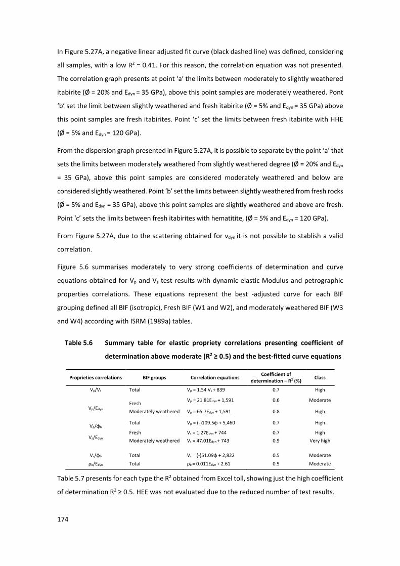
174
In Figure 5.27A, a negative linear adjusted fit curve (black dashed line) was defined, considering
all samples, with a low R2 = 0.41. For this reason, the correlation equation was not presented.
The correlation graph presents at point ‘a’ the limits between moderately to slightly weathered
itabirite (Ø = 20% and Edyn = 35 GPa), above this point samples are moderately weathered. Pont
‘b’ set the limit between slightly weathered and fresh itabirite (Ø = 5% and Edyn = 35 GPa) above
this point samples are fresh itabirites. Point ‘c’ set the limits between fresh itabirite with HHE
(Ø = 5% and Edyn = 120 GPa).
From the dispersion graph presented in Figure 5.27A, it is possible to separate by the point ‘a’ that
sets the limits between moderately weathered from slightly weathered degree (Ø = 20% and Edyn
= 35 GPa), above this point samples are considered moderately weathered and below are
considered slightly weathered. Point ‘b’ set the limits between slightly weathered from fresh rocks
(Ø = 5% and Edyn = 35 GPa), above this point samples are slightly weathered and above are fresh.
Point ‘c’ sets the limits between fresh itabirites with hematitite, (Ø = 5% and Edyn = 120 GPa).
From Figure 5.27A, due to the scattering obtained for νdyn it is not possible to stablish a valid
correlation.
Figure 5.6 summarises moderately to very strong coefficients of determination and curve
equations obtained for Vp and Vs test results with dynamic elastic Modulus and petrographic
properties correlations. These equations represent the best -adjusted curve for each BIF
grouping defined all BIF (isotropic), Fresh BIF (W1 and W2), and moderately weathered BIF (W3
and W4) according with ISRM (1989a) tables.
13Table 5.6 Summary table for elastic propriety correlations presenting coefficient of
determination above moderate (R2 ≥ 0.5) and the best-fitted curve equations
Proprieties correlations BIF groups Correlation equations Coefficient of determination – R2 (%) Class
Vp/Vs Total Vp = 1.54 Vs + 839 0.7 High
Vp/Edyn
Fresh Vp = 21.81Edyn + 1,591 0.6 Moderate
Moderately weathered Vp = 65.7Edyn + 1,591 0.8 High
Vp/ɸb Total Vp = (-)109.5ɸ + 5,460 0.7 High
Vs/Edyn Fresh Vs = 1.27Edyn + 744 0.7 High Moderately weathered Vs = 47.01Edyn + 743 0.9 Very high
Vs/ɸb
Total
Vs = (-)51.09ɸ + 2,822
0.5
Moderate
ρb/Edyn Total ρb = 0.011Edyn + 2.61 0.5 Moderate
Table 5.7 presents for each type the R2 obtained from Excel toll, showing just the high coefficient
of determination R2 ≥ 0.5. HEE was not evaluated due to the reduced number of test results.
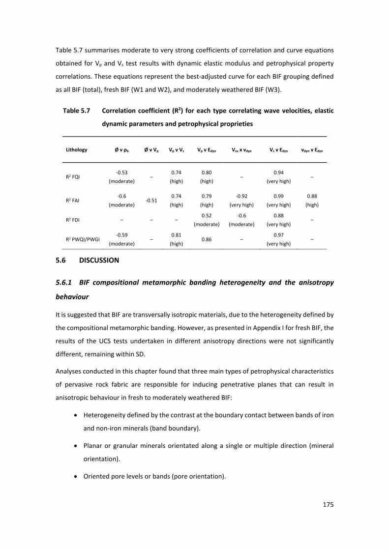
175
Table 5.7 summarises moderate to very strong coefficients of correlation and curve equations
obtained for Vp and Vs test results with dynamic elastic modulus and petrophysical property
correlations. These equations represent the best-adjusted curve for each BIF grouping defined
as all BIF (total), fresh BIF (W1 and W2), and moderately weathered BIF (W3).
14Table 5.7 Correlation coefficient (R2) for each type correlating wave velocities, elastic
dynamic parameters and petrophysical proprieties
Lithology Ø v ρb Ø v Vp Vp v Vs Vp v Edyn Vsv x νdyn Vs v Edyn νdyn v Edyn
R2 FQI -0.53
(moderate) –
0.74 (high)
0.80 (high)
– 0.94
(very high) –
R2 FAI -0.6
(moderate) -0.51
0.74 (high)
0.79 (high)
-0.92 (very high)
0.99 (very high)
0.88 (high)
R2 FDI – – – 0.52
(moderate) -0.6
(moderate) 0.88
(very high) –
R2 PWQI/PWGI -0.59
(moderate) –
0.81 (high)
0.86 – 0.97
(very high) –
5.6 DISCUSSION
5.6.1 BIF compositional metamorphic banding heterogeneity and the anisotropy
behaviour
It is suggested that BIF are transversally isotropic materials, due to the heterogeneity defined by
the compositional metamorphic banding. However, as presented in Appendix I for fresh BIF, the
results of the UCS tests undertaken in different anisotropy directions were not significantly
different, remaining within SD.
Analyses conducted in this chapter found that three main types of petrophysical characteristics
of pervasive rock fabric are responsible for inducing penetrative planes that can result in
anisotropic behaviour in fresh to moderately weathered BIF:
• Heterogeneity defined by the contrast at the boundary contact between bands of iron
and non-iron minerals (band boundary).
• Planar or granular minerals orientated along a single or multiple direction (mineral
orientation).
• Oriented pore levels or bands (pore orientation).
176
In addition to these fabric characteristics, the rock strength and anisotropy of each BIF type is also
influenced by chemical mineral affiliation (similar mineral hardens index and bulk density), similar
crystal sizes and the crystal contact surface, which ultimately is responsible for the roughness.
These fabric characteristics will exist in persistent and repetitive layers or bands of the fresh to
moderately weathered BIF that may define an anisotropy wherein the anisotropy index,
depending on P wave velocity propagation through the BIF samples, varies from isotropic (IVp =
1) to fairly anisotropic (IVp = 1.5).
Otherwise, discontinuities are not necessarily associated with the heterogeneity induced by
compositional metamorphic banding. They can be associated with slightly weathered levels with
higher porosity associated with structural features, such as fractures, and since these
discontinuities did not follow a pattern, they cannot be characterised as pervasive and persistent
anisotropy plans. However, when weathered they can form patterns of anisotropic-like surfaces
that cut thought the intact rock, especially from moderately weathered to highly weathered BIF.
This heterogeneity is characterised in different way for each of the BIF lithologies:
• HHE is a monomineralic (iron minerals) rock, with metamorphic heterogeneity banding
defined by interlayered bands of low or high Ø and normally associated with the
presence of tabular hematites and granoblastic hematite minerals associated with
different crystal sizes in each band. The IVp = 1.1 (fairly anisotropic) and Vp/Vs= 2.1.
• FAI, FDI and FQI are heterogeneous rocks with compositional metamorphic typical
itabirite banding defined by the repetition of iron and non-iron mineral bands that can
differ in size and crystal orientation. From the geomechanical perspective, both can
represent transverse anisotropy as defined by the three fabric characteristics (band
boundary, pore orientation, and mineral orientation), that in fact did not represent an
important anisotropy behaviour. The anisotropic index for FAI and FQI is IVp = 1.1 (fairly
anisotropic) and FDI IVp = 1.0 (isotropic) and Vp/Vs = 2 for all itabirites.
• For PWQI and PWGI, even with the higher total porosity observed (reaching 30%), the
anisotropic index (IVp = 1.5) is positioned at the limit between fair and moderately
anisotropic index. This higher relative anisotropic behaviour is also confirmed by the
lower relative wave velocity ratio (Vp/Vs = 1.8) from all BIF. However, it was found that
a significant increase in this index from fresh to moderately weathered BIF attributed
to the Ø increases and ρb decreases as the main changes occurring during the first
stages of the weathering. For BIF, the weathering processes, as already mentioned
177
uses the three pervasive planes as preferential paths for water percolation, inducing
leaching and mineralogical alteration (oxidation) reducing the parental intact rock
strength.
In summary, the HHE FAI and FQI showed fairly anisotropy index and FDI showed an isotropic
behaviour attributed to the non-band iron mineral composition (iron dolomites) that presents
higher P and S wave velocity when compared with quartz bands (closer to hematite). For
moderately weathered BIF, as the total porosity increases from 5% in average (fresh BIF) to
closer to 30%, this characteristic must control the anisotropic behaviour (and intact rock
strength). It is important to note that water content was not considered in this evaluation due
to the nature of samples and test preparation.
In evaluating Vp and Vs velocity propagation through BIF samples, the higher velocities were
obtained in general for β0° (along the banding heterogeneity) where the wave propagation is
especially faster, using preferentially the mineralogical continuity promoted by mineral
orientation and composition avoiding pore layers. Lower velocity was observed as expected at
β90° and β45° as the waves must cross porous and different minerals bands (non-iron and iron
bands). Although it was not possible to observe a typical U-shape (Jaeger 1960) curve due to the
lack of results in more than three anisotropy directions, it is possible to note that FQI, FAI, and
PWQI/PWGI presented similar asymmetric shape curves with upward concavity and maximum
at β0°. FDI, on the contrary, presented an almost symmetric shape curve with downward
concavity showing the largest velocities at β45°. This behaviour could be attributed to the low
difference between the P and S wave velocity along β45° compared with β0° of just 3%.
Band composition and thickness are important characteristics that define the BIF behaviour, the
intact rock strength and the elastic parameters. Where banding presents thicker layers of
non-iron minerals (e.g. carbonates or quartz bands), the result is a relatively less dense,
proportionally more porous rock. Also, the intact rock strength will be lower than other
specimens with more iron bands (thicker iron layers), which increases the iron content, reduces
porosity, and increases the ρb. This behaviour is remarkable for FDI where the increase in
non-iron bands results in a strength reduction even without a total porosity increase and Vp
decrease related to the petrophysical characteristics of the iron dolomite minerals already
discussed.
This evaluation is in accordance with Dalstra et al. (2003), who compare the Hamersley province
with other deposits worldwide and makes correlations of proto-ore assemblages with Fe grades
intermediate between the ore and the host BIF.
178
5.6.2 Correlations between wave velocity propagation, dynamic elastic, and
petrophysical proprieties
Considering all BIF types as an almost isotropic single group, the high coefficient of
determination between ρb, P and S wave velocity, total porosity and dynamic Young’s modulus
obtained for some lithotypes provide a reliable basis for defining parameters and property
correlations. Also, for describe the geological characteristics and geomechanical behaviour of
each lithotype. Even the lower coefficient of determination obtained for some lithotypes
represents useful data for describing rock type geomechanical behaviour.
The linear regression curves obtained for the petrophysical and geometrical correlations are
summarised and outlined in the following sections; first in general, considering the correlation
sets and then for BIF type.
Dynamic young’s modulus and P and S- wave velocity
Figures 5.20A and 5.20B, presented the expected linear positive correlations between Edyn and VP
and VS. The fresh and hard samples group presented VP R2 = 0.6 (moderate) and Vs R2 = 0.7 (high).
The moderately weathered samples group (W3 and W4) presented VP R2 = 0.8 (high) and
Vs R2 = 0.7 (high). The lower correlation for the fresh group is attributed to the low number of tests
from HHE.
Dynamic young’s modulus and bulk density
Figure 5.23A shows a linear positive regression curve adjusted to best fit expected for HHE
samples (higher ρb). For this reason, the correlation is moderate R2 = 0.5.
Rock samples with low ρb present lower VP and Vs compared with denser materials, that present
higher VP and Vs. This behaviour is expected and can be explained by the nature of the
compressional wave, which travels faster through more compact materials and low porosity
such as HHE. Although it is an expected result, experiments show weak to moderate correlation
for the entire group.
P and S wave velocity and total porosity
Figures 5.26A and 5.26C present, as expected, a linear negative correlation between total
porosity and P and S wave velocity. A single feet curve was obtained for the total porosity
correlation with VP R2 = 0.7 (high) and Vs R2 = 0.5 (moderate). The dependence of Vs on total
porosity is complex and multivariable. What can be suggested is the total porosity of fresh types
179
is quite low (Ø < 5%) and the bulk density varies from different compositional type influencing
the Vp and Vs correlations with the total porosity.
P and S wave velocity correlation
Figure 5.19 shows the expected linear correlation curve, with R2 = 0.7 (high).
As predicted in theory, using the Vp/Vs ratio it is possible to discriminate the rock type as
presented in Figure 5.19. Even though this study was carried out on a few samples, it was
possible to find Vp/Vs ratio values very close to those predicted by Pickett (1963), on average 2.1
to HHE, 2 to FAI and FDI, 1.9 to FQI, and 1.8 to PWQI and PWGI.
Due to the scatter obtained for νdyn it was not possible to establish valid correlations.
The correlation showed a similarity between different types of BIF that were grouped in Tables
5.5, 5.6 and 5.7 into three groups. The main characteristics of each group are described as follows.
• Hard hematitite group
The HHE high intact rock strength is mainly defined by the higher ρb (above 3.8 t/m3), low total
porosity (Ø < 5%) and small mineral size (0.001 mm to 0.08 mm). The higher Vp mean obtained
is 6,865 m/s and on average is 30% higher than the other BIF, and the Edyn > 125 GPa. The
heterogeneous metamorphic banding is represented by layers with higher total porosity
interlayered with more massive ones, conditioned by mineral and pore orientation inducing fair
anisotropy.
Since the anisotropy effects are not important for HHE, the high standard deviation noted could
be attributed to the reduced number of tests.
• Fresh to slightly weathered itabirites group
Fresh itabirite is the most common BIF lithotype, presenting compositional metamorphic
banding conditioned by concentrated quartz and/or iron dolomite bands interplayed with iron
bands representing the typical itabirite heterogeneity. The high intact rock strength is mainly
defined by the typical bulk density (3.2 t/ m3 ≤ ρb ≤ 3.8 t/m3) and typical total porosity (W2 - 10%
≥ ɸ ≥ 3% - W1). Vp varies from 3,800 m/s to 6,200 m/s and Edyn from 35 GPa to 125 GPa. The
higher percentage of porous layers are concentrated on non-iron bands or at the contact
between bands inducing some fair anisotropy parallel to the typical compositional metamorphic
banding identified in great depths.
180
The higher heterogeneity in crystal size observed in this type seems not to influence by the
anisotropic effects measured from Vp and Vs values as values the IVP are similar from HHE (more
homogeneous crystal size type,).
The anisotropy degree is low. Observed is a different anisotropy behaviour for FDI (Rc=2),
partially attributed to the presence of iron dolomite minerals with lower mineral hardness as
compared with quartz and similar Vp and Vs velocities, compared with hematite. Nevertheless, it
must be considered that the iron dolomite bands contributed to reduce the strength and the
elastic parameters even keeping high Vp and Vs and Ø values of this type.
• Moderately weathered itabirites group
PWQI and PWGI present the same geological characteristics compared with fresh itabirites. It is
considered the first weathering product from fresh itabirites (weathering grade changed from
W1/W2 to W3/W4). IN shallower depths, this weathering change is easily identified in field and
laboratory samples. The lower intact rock strength is mainly defined by the lower bulk density
(ρb < 3.2 t/m3) higher total porosity (Ø > 22%), lower P wave velocity with values below
3,800 m/s, and Edyn lower than 35 GPa. These higher percentages of porous layers are
concentrated in both non-iron and iron bands, and mainly at the contact between bands
inducing some fair to moderately anisotropy index parallel to the compositional metamorphic
banding (higher from all BIF). They are caused by weathering (leaching of quartz and
recrystallising different iron ore oxides and hydroxides). Increasing percentages of the layers
potentially generate preferential weathering paths that can increase the anisotropy and change
to moderately weathered lithotypes.
Lower intact rock strength is mainly defined by the high pore content. The higher heterogeneity
in crystal size observed in this type seems to influence the strength and anisotropy mainly due
to the lack of cementation for PWQI. The intact rock strength observed for PWGI due to the
goethite cementation normally observed in this type are higher when compared with the PWQI.
The leaching effectiveness on iron dolomite bands for FDI results in the absence of moderately
weathered (W3 and W4) rocks in the weathering profile. Contrarily, from quartz based itabirites
(FAI and FQI), as the leaching is not efficient it is present in the weathering profile a full range of
the weathering grade from W1 to W6 according to ISRM (1989a) tables.
Even with several attempts to reduce data dispersion, some parameters showed high SD. This may
represent the natural dispersion promoted by intrinsic geological features, or by the observed
higher anisotropic effects especially for FDI, PWQI and PWGI.
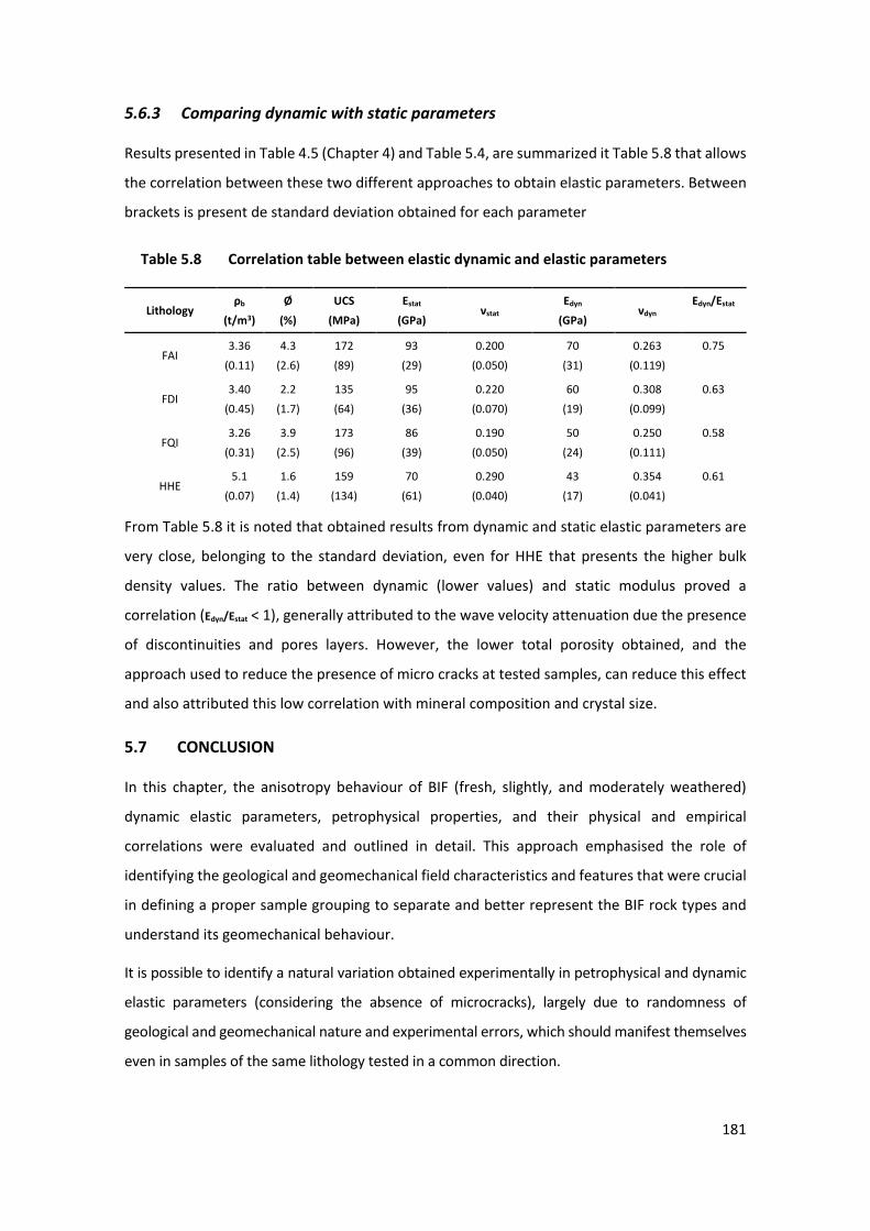
181
5.6.3 Comparing dynamic with static parameters
Results presented in Table 4.5 (Chapter 4) and Table 5.4, are summarized it Table 5.8 that allows
the correlation between these two different approaches to obtain elastic parameters. Between
brackets is present de standard deviation obtained for each parameter
15Table 5.8 Correlation table between elastic dynamic and elastic parameters
Lithology ρb
(t/m3) Ø
(%) UCS
(MPa) Estat
(GPa) νstat
Edyn
(GPa) νdyn
Edyn/Estat
FAI 3.36
(0.11) 4.3
(2.6) 172 (89)
93 (29)
0.200 (0.050)
70 (31)
0.263 (0.119)
0.75
FDI 3.40
(0.45) 2.2
(1.7) 135 (64)
95 (36)
0.220 (0.070)
60 (19)
0.308 (0.099)
0.63
FQI 3.26
(0.31) 3.9
(2.5) 173 (96)
86 (39)
0.190 (0.050)
50 (24)
0.250 (0.111)
0.58
HHE 5.1
(0.07) 1.6
(1.4) 159
(134) 70
(61) 0.290
(0.040) 43
(17) 0.354
(0.041) 0.61
From Table 5.8 it is noted that obtained results from dynamic and static elastic parameters are
very close, belonging to the standard deviation, even for HHE that presents the higher bulk
density values. The ratio between dynamic (lower values) and static modulus proved a
correlation (Edyn/Estat < 1), generally attributed to the wave velocity attenuation due the presence
of discontinuities and pores layers. However, the lower total porosity obtained, and the
approach used to reduce the presence of micro cracks at tested samples, can reduce this effect
and also attributed this low correlation with mineral composition and crystal size.
5.7 CONCLUSION
In this chapter, the anisotropy behaviour of BIF (fresh, slightly, and moderately weathered)
dynamic elastic parameters, petrophysical properties, and their physical and empirical
correlations were evaluated and outlined in detail. This approach emphasised the role of
identifying the geological and geomechanical field characteristics and features that were crucial
in defining a proper sample grouping to separate and better represent the BIF rock types and
understand its geomechanical behaviour.
It is possible to identify a natural variation obtained experimentally in petrophysical and dynamic
elastic parameters (considering the absence of microcracks), largely due to randomness of
geological and geomechanical nature and experimental errors, which should manifest themselves
even in samples of the same lithology tested in a common direction.
182
As noted, geological features induce some dispersions of the results, since they may have
different microstructural variations in fabric, affected by rock heterogeneity and early influence
of weathering, inducing in some rock types little, but not irrelevant anisotropy effects, and
variations in the petrophysical properties of the samples (e.g. ρb and Øb). Even so, using several
methodologies (samples separation and statistical approach) it was possible to group similar
types verifying reliable trends of a correlation based on P and S wave velocity propagation
(dynamic parameters).
For HHE, FAI and FQI, the anisotropy index is fair, and FDI behave as a moderately anisotropic
material due to the high P and S wave velocities obtained for iron dolomitic minerals bands.
A moderately IVP was also identified for PWQI and PWGI, mainly caused by the total porosity
increase and ρb decrease (more weathered type) noted in these types.
Considering the typical heterogeneity defined by the compositional metamorphic banding for
itabirite, evaluations of macroscopic and microscopic characteristics revealed that there is very
little effective anisotropic behaviour, as the anisotropic index varies from isotropic to little
anisotropy for fresh and slightly weathered BIF. However, moderately weathered BIF presented
moderately anisotropy index, and for these material, transverse anisotropy must be considered.
Three main petrophysical characteristics were found to be responsible for inducing penetrative
planes that could result in this little anisotropy observed are:
• Contact between bands of iron and non-iron minerals, which define the itabirite
compositional metamorphic banding (heterogeneity).
• Planar or granular minerals orientated along a single direction or multiple directions
(mineral orientation).
• Porous layers (total porosity percentage and orientation) which define the hematite
heterogeneity.
In general, the low strain and low metamorphic grade (green schist) observed along the western
side of the Iron Quadrangle resulted on the relatively simple mineralogical assemblages of the
BIF and creating a poorly orientated fabric with small mineral size, that imposed fair anisotropy
on the intact rock generally observed in great depths where the enrichment and weathering
process did not reach. This behaviour can be attributed to the presence of minerals with similar
mineralogical strength (mineral hardness), bulk density, and strong contacts between the
individual crystal defined by BIF fabric. The relationships evaluated and the adjusted regression
183
curves provided equations that can be used to estimate and characterise each lithotype and the
difference from fresh to moderately weathered BIF types.
The study also indicates that the effects of the level of weathering directly influence the dynamic
elastic and rock proprieties for different kinds of BIF. Anisotropy is responsible for little
variations, mainly for FDI, HHE, FAI and FQI and moderately for PWQI and PWGI. This behaviour
is defined by using dynamic and non-destructive methods using P and S wave velocity
propagation, supported by total porosity, and bulk density measurements.
In general, ρb and Ø are the main petrophysical properties that control the dynamic elastic
behaviour, with a strong contrast between fresh from moderately weathered rocks, easily noted
from Vp and Vs results. The high correlation determination and empirical correlation obtained for
each lithotype proved to be a useful approach to describe the total porosity and Edyn with ρb. This
behaviour is noted when comparing dynamic with static elastic modules where were obtained a
correlation Edyn/Estat < 1 showing wave velocity attenuation mainly induced by the samples
inherent microcracking (noted for HHE), pores layers, mineral composition and fabric.
The techniques used to determine the total porosity, using a qualitative micro thin section
evaluation (Øb) correlated with laboratory tests (Ø), even with inconsistence related to the
measurements techniques, showed to be reliable to define the ranges of each fresh to moderate
lithotype. Total porosity is the petrophysical property that presents, as expected, inverse linear
correlation with S and P wave velocity, and this correlation can be used to estimate the
weathering grade and, indirectly, the iron content as proposed in the Appendix I. Bulk density is
also appropriate to estimate Edyn correlations. Attention must be taken to FDI correlations, due
to the presence of iron dolomites minerals that induce changes in some correlations.
The evaluated assemblage of itabirites and hematitites could be regrouped into three groups of
similar behaviour and relative parameters definition:
• PWQI and PWGI (moderately weathered itabirites group), with lower wave velocities,
Edyn values and ρb, and higher total porosity.
• FQI, FDI and FAI (fresh to slightly weathered itabirites group), with typical high range
for wave velocities and Edyn values and moderate ρb, and low total porosity.
• HHE (hard hematitite group), with higher wave velocity, Edyn values, and ρb, and very
low total porosity.
These groups are directly associated with the intact rock strength, and the weathering process
increase is mainly associated with the total porosity increase for FAI and FQI grading from fresh
184
(W1) to slightly (W2) and finally to moderately weathered (W3/W4) types. In the same context,
this grading is not observed for FDI (lack of moderately weathered types), resulting in
weathering profile with just two different weathering horizons – fresh (W1/W2) and completely
weathered (W5/W6). This behaviour is attributed to the efficiency of the leaching process
(which decreases with depth), with is more prone for FDI than FQI and FAI. This behaviour is in
accordance with the distinct weathering profiles observed in Iron Quadrangle iron mines as
presented in Appendix I and II.
The use of empirical correlations graphs and equations to predict dynamic elastic and intact rock
strength parameters and petrophysical properties has proved to be a reliable methodology to
estimate the geomechanical characteristics that are directly associated with lithotype.
Additionally, the weathering grade and heterogeneity were defined as important features that
control anisotropy, bulk density, elastic parameters and, ultimately, the intact rock strength of the
BIF.
The field geological and geomechanical investigations and laboratory tests undertaken during
the research programme enabled to assess the effect of physical heterogeneity and anisotropy
on the geomechanical properties of the BIF deposits in the western side of Brazil’s Iron
Quadrangle and develop procedures that will optimise pit slope design, promote a better
understanding of potential slope failure mechanisms and reduce the risk of slope failure – gains
that will help Vale and other iron ore mines improve the operational productivity and safety of
their iron ore mines.
185
CHAPTER 6. WEAK ROCK BEHAVIOUR OF HIGHLY TO COMPLETELY
WEATHERED BANDED IRON FORMATIONS FROM IRON QUADRANGLE –
BRAZIL
This chapter presents the third unpublished manuscript.
ABSTRACT
Weathering is defined as the most important factor responsible for reducing the original high
intact rock strength and converting the hard itabirite rocks into weak rocks, which display a
variety of soil-like properties, while in some cases retaining the relic structures comprising mainly
the heterogeneity derived from the original compositional metamorphic banding. As a
consequence, strength and petrophysical parameters, and other physical characteristics are
significantly affected.
In the deep weathering profiles, normally observed in Brazilian iron ore mines, there are
predominantly saprolite and residual soil in the first four hundred metres from surface.
Additionally, a climate with high pluviometry during long periods of the year and a cycle of
discharge and recharge by the rainy season impose alternating periods of saturated and
unsaturated conditions in near surface and subsurface within the banded iron formations (BIF).
For these weathered materials, saturated soil mechanics concepts dominate slope failure
analyses and slope design evaluations not only for residual soil materials, but also for weak and
completely weathered BIF for iron ore mines in the Iron Quadrangle, Brazil. These studies were
supported by laboratory tests and previous experience and has proven to be adequate to back-
analyse several observed failure mechanisms. However, the approach was not sufficient in itself
to avoid global failures and has therefore led to the adoption of very conservative slope designs,
including leaving large buttresses of rich ore at the toe of slopes.
The purpose of this chapter is to evaluate field geological petrophysical and geotechnical
characteristics and to compare with laboratory tests that determine the saturated and
unsaturated shear strengths as a means of describing the geomechanical behaviour of four
soil-like highly to completely weathered BIF types. These completely weathering typologies are
locally termed weathered argillaceous itabirite, weathered quartzitic itabirite, weathered
goethitic itabirite and weak hematitite. These materials represent more than 70% of the mined
ore in Vale mines.
186
The studies undertaken included geological and geotechnical field investigation, testing to assess
in situ and laboratory (permeability, natural moisture content) particle size distribution,
Atterberg limits, drained and undrained triaxial and direct shear tests, soil–water characteristic
curves and bulk density, as well as petrographic thin section analyses for each type. From these
investigations, petrophysical characteristics, soil classification and shear strengths (saturated
and unsaturated) parameters were obtained, and shear strengths with respect to matric suction
were evaluated, considering the anisotropic effects induced by compositional metamorphic
banding observed in these material types.
Results show that mineralogical composition, bulk density, and total porosity are strongly
associated, leading to distinct shear strength properties as indicated by the Unified Soil
Classification System (USCS) soil classification and plasticity chart. Anisotropy ratio is low for
weathered argillaceous, quartzitic and goethitic itabirites, and the weak hematitite is isotropic.
Saturated strength parameters increase from the lower-strength for weathered argillaceous
itabirites to weathered quartzitic and goethitic itabirites, with the highest strength observed in
the weak hematitite. The mineral fabric, mineralogy and higher total porosity layers can induce
ductile failures at low stress level, and at higher stress levels could induce brittle failures as a
result of the post-peak loss of strength (strain softening).
Unsaturated direct shear tests show that shear strengths involving matric suction exhibit
unsaturated friction angles higher than the saturated direct shear test as a result of the suction
effect playing a role in the apparent cohesion. This phenomenon is associated with the dilatation
at low stress levels induced by slightly higher clay content of the weathered argillaceous itabirite,
presence of kaolinite and gibbsite. For this reason, unsaturated behaviour must be considered
for less conservative slope stability analyses, essentially for temporary slopes during the dry
season and in the near surface transient unsaturated zones.
It is possible to classify the weak, highly to completely weathered BIF as a saprolite to residual
soil material of thoroughly weathered rock that has not been transported. As such, the BIF can
be defined as immature residual soils, i.e. weak rocks, mainly composed of very dense sand and
silt materials. Variations in secondary clay and clast contents also define different behaviour,
highly depending on the stress level. In general, at low stress levels (below 400 kPa) BIF behave
like loose sandy material, while for high stress levels (above 400 kPa) they behave like dense
sandy material. However, variations in total porosity, bulk density and mineralogy composition
can change these behaviours.
187
6.1 INTRODUCTION
In the Iron Quadrangle mines of Brazil, banded iron formations (BIF) are divided into ‘itabirite’,
the low-grade ore, and ‘hematite’, the high-grade ore. The genesis of these lithologies is
controversial, but it is assumed that hypogene and supergene processes were responsible for
the iron concentration that changes itabirites into hematitites. In addition, it is understood that
tectonic events, as well as weathering, were responsible for reducing hard itabirites (considered
original proto-ore) to weak weathered materials (saprolite) and are also responsible for
generating the deep weathered profiles commonly observed in iron ore mines.
In this chapter, the influence of the weathering on the shear strength behaviour of highly to
completely weathered BIF observed at surface and in deeper weathering profiles is evaluated.
The four weak material types studied represent more than 70% of mined ore and are classified
based on the main non-iron mineral band into weathered argillaceous itabirite (WAI), weathered
quartzitic itabirite (WQI), weathered goethitic itabirite (WGI) and weak hematitite (WHE).
As presented in Lao (2013), for current slope design, the effect of unsaturated strength and flow
on the evaluation of slope stability in residual soils has not usually been considered. This is
mainly because the mechanics of unsaturated soils are poorly understood and neglecting the
strength increase due to partial saturation is a conservative approach. Also, conventional
laboratory testing is usually carried out under saturated conditions. Consequently, this approach
probably leads to a difference between real conditions and the analytical results. Especially for
the residual soils in tropical or subtropical regions where the groundwater table is usually deep,
evapotranspiration often potentially exceeds infiltration and groundwater tables are often low
because of the climatic conditions and dense vegetation, resulting in an unsaturated top layer
with continuous air in the voids above the watertable.
In the Iron Quadrangle iron ore mines, these materials are commonly observed at depths of up
to 400 m, and this zone is normally called the superficial weathered profile. The slope stability
approach and failure mechanism analyses in this profile are based on saturated soil mechanics
principles. While this approach has been largely satisfactory, there are several other key
geotechnical issues that are still not well understood, and that appear to have caused large slope
failures that have resulted in significant disruption to mining. Otherwise, this approach has been
shown to be very conservative, mainly for short-term slopes above the water level leading to
the maintenance of larger safety berms in slope toes blocking part of the ore reserve.
It is also recognised that failure mechanisms in weak rock slopes are controlled mainly by intact
rock shear strength and locally due to anisotropic effects conditioned by the compositional
188
metamorphic banding, as well as secondary factors such as structural control and groundwater.
The situation is particularly challenging when considering the stratigraphic position and/or
tectonic settings of these weak and weathered rocks, which are very often located at the toe of
high slopes, where the stress is concentrated, and few studies have been conducted on these
effects.
The current approach used to support slope stability analyses in these types of weak rocks (with
soil behaviour) is based on limit equilibrium analyses using the Mohr–Coulomb failure criterion
and effective shear strength parameters of the saturated materials. The shear strength
parameters are normally supported by a limited number of laboratory tests, mainly saturated
tests (drained triaxial and direct shear tests), supported by adapted rock mass classifications.
While this approach has been mostly adequate to minimise slope stability problems, it would
appear from experience that they are conservative. Despite that, there have been examples of
large slope failures not captured by these design approaches that have had significant negative
impacts for mine production. In this matter, this charter evaluated approaches that consider the
permeability and porewater pressure effects in unsaturated slope stability analyses in order to
consider the real unsaturated soil slope behaviour.
In addition, some classical soil mechanics parameters such as total porosity, bulk density,
particle size distribution, Atterberg limits, mineral shape and mineralogy have not been properly
evaluated and considered in relation to the observed slope stability analyses and failure
mechanism behaviour and evaluations. Due to the difficulties associated with sample
preparation, representativeness and testing, a correct evaluation of these characteristics and
parameter correlations remain a key challenge for a complete behaviour understanding.
In summary, this section presents a brief review of the geological setting weak BIF and the key
geological and geotechnical characteristics of studied material types are presented. The
petrophysical characterisation and material parameter definitions are based on Vale’s
geotechnical laboratory test database, as well as WHE petrographic thin sections from Costa
(2009) and laboratory tests specially undertaken to determine bulk density, natural moisture
content, particle size distributions, Atterberg limits, soil–water characteristic curves, direct
shear and triaxial tests (drained and undrained) and permeability (field and laboratory). These
test results were summarised and evaluated to determine correlations between petrophysical
characteristics and geomechanical parameters. The chapter also discusses and arrives at
conclusions regarding the relationship between saturated and unsaturated shear strength
parameters and presents a bilinear envelope with respect to a matric suction for each typology.
189
Finally, the implications of these test results on pit slope stability are discussed and presented
in Appendix II.
6.2 OBJECTIVES AND APPROACHES
The aim of this section is to evaluate the geomechanical behaviour, shear strength parameters
and petrophysical characteristics based on laboratory tests and geological/geotechnical field
evaluation for highly to completely weathered BIF types. The research aims to address some key
statements summarised as follows:
• Identify and compare the differences in the geological and geomechanical behaviour,
and shear strength characteristics from different highly to completely weathered BIF
types.
• Evaluate the heterogeneity, provided by the compositional metamorphic banding, and
the importance of the anisotropy in the geomechanical behaviour and shear strength.
• Determine the parameters and evaluate the saturated and unsaturated behaviour for
completely weathered BIF.
Secondly, the behaviour characterisation is evaluated with regard to the importance of the
porewater pressure and suction effects in these soil-like materials.
The chapter is focused on the shear strength properties, as well as assessing the effect of
heterogeneity and anisotropy to establish a practical correlation as a function of the
mineralogical composition, fabric, bulk density, permeability and other petrophysical
characteristics. It does not include discontinuity characterisation.
This section is part of a PhD research project undertaken by the lead author at the Australian
Centre for Geomechanics, School of Civil, Environmental and Mining Engineering, The University
of Western Australia, sponsored by Vale S.A. The thesis research investigates the complete
weathering profile characteristics, from fresh and hard to weak and completely weathered BIF
from several Vale iron ore mine sites.
The studied mines are part of Vale’s south ferrous division and comprise of five mines (Figure
6.1) located in the centre of Minas Gerais state, Brazil, named Capão Xavier (CPX), Tamanduá
(TAM), Capitão do Mato (CMT), Sapecado (SAP) and Jangada (JGD).
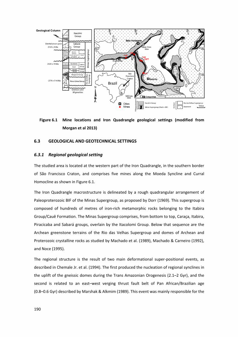
190
51 Figure 6.1 Mine locations and Iron Quadrangle geological settings (modified from
Morgan et al 2013)
6.3 GEOLOGICAL AND GEOTECHNICAL SETTINGS
6.3.1 Regional geological setting
The studied area is located at the western part of the Iron Quadrangle, in the southern border
of São Francisco Craton, and comprises five mines along the Moeda Syncline and Curral
Homocline as shown in Figure 6.1.
The Iron Quadrangle macrostructure is delineated by a rough quadrangular arrangement of
Paleoproterozoic BIF of the Minas Supergroup, as proposed by Dorr (1969). This supergroup is
composed of hundreds of metres of iron-rich metamorphic rocks belonging to the Itabira
Group/Cauê Formation. The Minas Supergroup comprises, from bottom to top, Caraça, Itabira,
Piracicaba and Sabará groups, overlain by the Itacolomi Group. Below that sequence are the
Archean greenstone terrains of the Rio das Velhas Supergroup and domes of Archean and
Proterozoic crystalline rocks as studied by Machado et al. (1989), Machado & Carneiro (1992),
and Noce (1995).
The regional structure is the result of two main deformational super-positional events, as
described in Chemale Jr. et al. (1994). The first produced the nucleation of regional synclines in
the uplift of the gneissic domes during the Trans Amazonian Orogenesis (2.1–2 Gyr), and the
second is related to an east–west verging thrust fault belt of Pan African/Brazilian age
(0.8–0.6 Gyr) described by Marshak & Alkmim (1989). This event was mainly responsible for the
191
deformational gradient in the western side with low strain and green schist metamorphic grade,
as described by Hertz (1978). The geological settings are also shown in Figure 6.1.
The Iron Quadrangle BIF are heterogeneous banded rocks presenting a millimetre to centimetre
rhythmic alternation of iron and non-iron minerals which have been recrystallised to quartz from
original chert or jasper bands. Compositional metamorphic banding is the most typical
characteristic and defines a strong heterogeneity. This variation could be controlled by the
original sedimentary bedding, tectonic setting, metamorphic grade, hydrothermal or supergene
processes. However, the superimposition of these processes causes partial or total mineralogical
and textural changes, making it difficult to identify the heterogeneity control.
Dorr (1969) defined, for this type of iron deposit, two main lithologies: hematite or hematitite,
the high-grade ore (Fe≥ 64%), and itabirite, the low-grade ore (Fe<64%), which is divided into
three compositional lithotypes denominated by the main non-iron minerals: quartzitic,
dolomitic and amphibolitic itabirites. From these proto-ores, tectonic, metamorphic, and
weathering processes changed them in different ways and magnitudes, resulting in a multiple
setting of iron ore typology which are subdivided by the weathering profile level in horizons and
zones, rock strength and structural setting.
The origin of itabirites and associated high-grade hematite orebodies remains controversial, and
several works have been produced on this topic (Spier et.al 2003). For the genesis of the friable
orebodies some authors agree on a supergene process and residual itabirite enrichment, with
leaching of the gangue minerals by surface waters. For these orebodies, the 40Ar/39Ar dating
of manganese minerals in Vale mines, presented by Spier (2005) and Spier et al. (2006), suggest
that weathering and the mineralisation period occurred between 61.5 ± 1.2 Myr to 14.2 ±
0.8 Myr, reaching the peak process in 51 Myr. This suggests a tertiary mineralisation (66 Myr),
and after this period the weathering may not have substantially affected the weathering profile.
6.3.2 Banded iron formation geological settings
In Vale mines, hematitite and the three compositional itabirites are subdivided according to rock
hardness by a technical crusher laboratory test used to simulate the industrial process. This test
consists of crushing a known mass of sample to less than 31.5 mm, then sieving it through a 6.35
mm sieve, resulting in three main types: hard or compact (more than 50% above 6.35 mm);
medium hard or semi-compact (50% to 25% above 6.35 mm); and weak or friable (less than 25%
above 6.35 mm). Using this approach, Vale’s crusher test has been used as a guide to identify
the weathering level and the strength index (hardness), with classification into hard (R5 or R6)
192
are associated to fresh (W1) to slightly weathered material (W2); medium hard (R4 and R3),
representing moderately (W3) to highly weathered material (W4); and weak (R2 to R0),
representing completely weathered (W5) to residual soil (W6) as presented in ISRM (1981)
tables.
As suggested by the new strength table present in Martin & Stacey (2018), the strength index of
the studied materials is classified as lower-strength varying from R2 to R0, and the weathering
grade varies from highly weathered (W4) to residual soil (W6). Average uniaxial compressive
strength (UCS) values of these materials are below 1 MPa, with the upper boundary, for
moderately weathered materials, reaching 10 MPa and defined as R2+. The lower boundary
overlaps soil classifications corresponding to a very stiff soil (S5) to hard soil (S6) which places
these materials in a boundary zone between rock and soil behaviour.
For the hydrogeological characteristics, the WHE, the WQI and the WGI behave as granular
aquifers with low primary but high secondary porosities and storage coefficients, which reduces
in less fractured zones. Due to the relatively high percentage of clay minerals, the WAI behaves
as an aquitard and can locally modify the aquifer flow or generate confined aquifers.
Additionally, due to annual rainfalls of between 1,500 mm to 1,700 mm with approximately 90%
of annual precipitation concentrated between October to March (summer), superficial aquifers
(transient aquifers) can occur, closely associated to the climate seasonality fluctuation (order of
tens of metres) (Reboita et al. 2015). Conversely, the deep aquifer is minimally affected by the
climate seasonality (metric order). However, it is strongly affected by mine dewatering.
The main geological and geotechnical characteristics obtained from previous reports and the
database of these types (lithotypes) can be described as follows.
Weak hematitite
Weak hematitite (WHE) is the main supergene ore type and the most extensive and richest in
iron ore mines. The original term ‘weak hematite’, defined for this type, was changed to
hematitite as suggested by several authors in order to define the rock type differently to mineral
type. It consists of thin (millimetric to centimetric) opaque/dark grey colour layers of hematite
and martite, with low apparent cohesion (friable) and high visual total porosity (Øb) alternating
with more cohesive layers of dark metallic bands of hematite and martite with higher relative
strength and lower Øb.
The Øb varies significantly from 25% to 30%, according to Costa et al. (2009), or even higher,
from 29% to 37% according to Ribeiro (2003). This lithotype presents a heterogeneity well
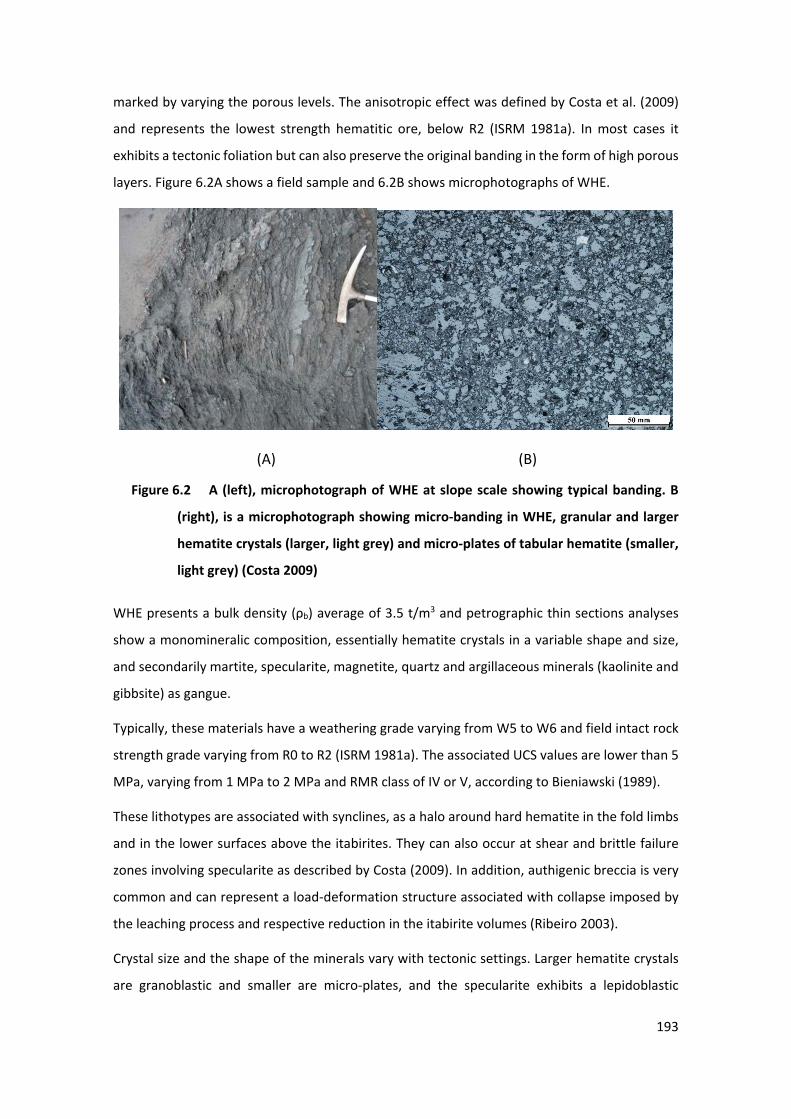
193
marked by varying the porous levels. The anisotropic effect was defined by Costa et al. (2009)
and represents the lowest strength hematitic ore, below R2 (ISRM 1981a). In most cases it
exhibits a tectonic foliation but can also preserve the original banding in the form of high porous
layers. Figure 6.2A shows a field sample and 6.2B shows microphotographs of WHE.
(A) (B)
52 Figure 6.2 A (left), microphotograph of WHE at slope scale showing typical banding. B
(right), is a microphotograph showing micro-banding in WHE, granular and larger
hematite crystals (larger, light grey) and micro-plates of tabular hematite (smaller,
light grey) (Costa 2009)
WHE presents a bulk density (ρb) average of 3.5 t/m3 and petrographic thin sections analyses
show a monomineralic composition, essentially hematite crystals in a variable shape and size,
and secondarily martite, specularite, magnetite, quartz and argillaceous minerals (kaolinite and
gibbsite) as gangue.
Typically, these materials have a weathering grade varying from W5 to W6 and field intact rock
strength grade varying from R0 to R2 (ISRM 1981a). The associated UCS values are lower than 5
MPa, varying from 1 MPa to 2 MPa and RMR class of IV or V, according to Bieniawski (1989).
These lithotypes are associated with synclines, as a halo around hard hematite in the fold limbs
and in the lower surfaces above the itabirites. They can also occur at shear and brittle failure
zones involving specularite as described by Costa (2009). In addition, authigenic breccia is very
common and can represent a load-deformation structure associated with collapse imposed by
the leaching process and respective reduction in the itabirite volumes (Ribeiro 2003).
Crystal size and the shape of the minerals vary with tectonic settings. Larger hematite crystals
are granoblastic and smaller are micro-plates, and the specularite exhibits a lepidoblastic
194
texture. In size, these iron minerals vary from 0.005 mm to 0.5 mm, with a maximum of 1 mm
(Rosière 2005) (Figure 6.2B).
Heterogeneity is characterised by the orientation of crystals, porosity variations and void
alignments. In some cases, it is possible to see two orientations (foliation and banding). Using
these micro characteristics, Costa (2009) defines three distinct sub-types of WHE:
• Subtype banded: Composed of by centimetric banding layers with less apparent
cohesion interfingered with more cohesive layers. They occur in the fold limbs and
above the itabirite, with low deformation and constituting the main type in open pits
in terms of extent. Crystal orientation is determined by metamorphic recrystallisation,
and heterogeneity is defined by the interfingered layers, with porous and tabular
hematite determining an anisotropy direction, and a medium void ratio commonly
occurring in areas with low deformation. The micro-bedding typically involves less
porous granular crystals interfingered with micro-plates of more porous hematite, as
illustrated in Figure 6.3A.
• Subtype foliated: Millimetric foliation and specularite are responsible for apparent
strong anisotropy, low lateral extension, low apparent cohesion and low porosity, are
associated with shear zones. Specularite minerals are concentrated in high
deformation areas (length increased by deformation and oriented), predominated as
a granuloblastic to lepidoblastic texture, defining an oriented foliation especially at
tabular and specular hematite crystals. All of this is shown in Figure 6.3B.
• Subtype brecciated: Typical bimodal composition with ‘clast’ layers with very low
apparent cohesion and isotropic, predominately formed by highly porous granular
crystals of hematite, and ’matrix’ layers dominated by macro-plates of low-porosity
hematite. The breccias are associated with collapsed structures (not tectonic
autogenic breccias) as defined by Ribeiro (2003) and fault zones; Figure 6.3C features
this description.
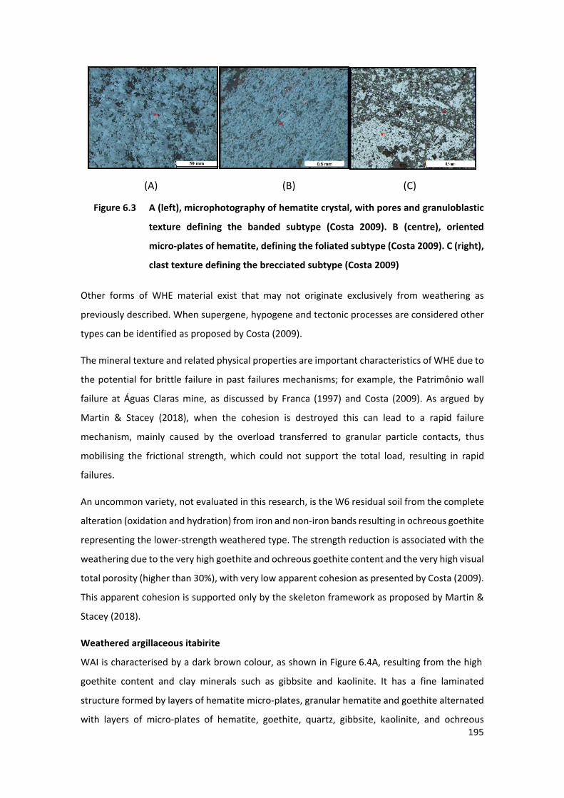
(A) (B) (C)
53 Figure 6.3 A (left), microphotography of hematite crystal, with pores and granuloblastic
texture defining the banded subtype (Costa 2009). B (centre), oriented
micro-plates of hematite, defining the foliated subtype (Costa 2009). C (right),
clast texture defining the brecciated subtype (Costa 2009)
Other forms of WHE material exist that may not originate exclusively from weathering as
previously described. When supergene, hypogene and tectonic processes are considered other
types can be identified as proposed by Costa (2009).
The mineral texture and related physical properties are important characteristics of WHE due to
the potential for brittle failure in past failures mechanisms; for example, the Patrimônio wall
failure at Águas Claras mine, as discussed by Franca (1997) and Costa (2009). As argued by
Martin & Stacey (2018), when the cohesion is destroyed this can lead to a rapid failure
mechanism, mainly caused by the overload transferred to granular particle contacts, thus
mobilising the frictional strength, which could not support the total load, resulting in rapid
failures.
An uncommon variety, not evaluated in this research, is the W6 residual soil from the complete
alteration (oxidation and hydration) from iron and non-iron bands resulting in ochreous goethite
representing the lower-strength weathered type. The strength reduction is associated with the
weathering due to the very high goethite and ochreous goethite content and the very high visual
total porosity (higher than 30%), with very low apparent cohesion as presented by Costa (2009).
This apparent cohesion is supported only by the skeleton framework as proposed by Martin &
Stacey (2018).
Weathered argillaceous itabirite
WAI is characterised by a dark brown colour, as shown in Figure 6.4A, resulting from the high
goethite content and clay minerals such as gibbsite and kaolinite. It has a fine laminated
structure formed by layers of hematite micro-plates, granular hematite and goethite alternated
with layers of micro-plates of hematite, goethite, quartz, gibbsite, kaolinite, and ochreous 195
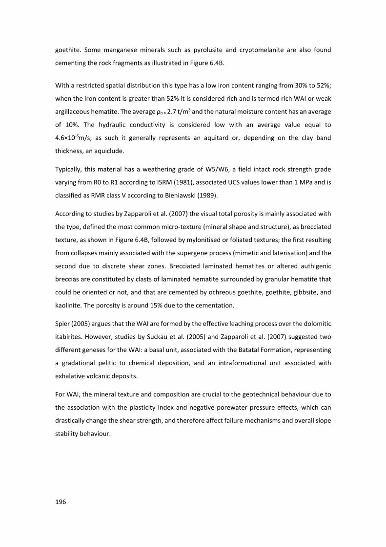
196
goethite. Some manganese minerals such as pyrolusite and cryptomelanite are also found
cementing the rock fragments as illustrated in Figure 6.4B.
With a restricted spatial distribution this type has a low iron content ranging from 30% to 52%;
when the iron content is greater than 52% it is considered rich and is termed rich WAI or weak
argillaceous hematite. The average ρb = 2.7 t/m3 and the natural moisture content has an average
of 10%. The hydraulic conductivity is considered low with an average value equal to
4.6×10⁻⁶m/s; as such it generally represents an aquitard or, depending on the clay band
thickness, an aquiclude.
Typically, this material has a weathering grade of W5/W6, a field intact rock strength grade
varying from R0 to R1 according to ISRM (1981), associated UCS values lower than 1 MPa and is
classified as RMR class V according to Bieniawski (1989).
According to studies by Zapparoli et al. (2007) the visual total porosity is mainly associated with
the type, defined the most common micro-texture (mineral shape and structure), as brecciated
texture, as shown in Figure 6.4B, followed by mylonitised or foliated textures; the first resulting
from collapses mainly associated with the supergene process (mimetic and laterisation) and the
second due to discrete shear zones. Brecciated laminated hematites or altered authigenic
breccias are constituted by clasts of laminated hematite surrounded by granular hematite that
could be oriented or not, and that are cemented by ochreous goethite, goethite, gibbsite, and
kaolinite. The porosity is around 15% due to the cementation.
Spier (2005) argues that the WAI are formed by the effective leaching process over the dolomitic
itabirites. However, studies by Suckau et al. (2005) and Zapparoli et al. (2007) suggested two
different geneses for the WAI: a basal unit, associated with the Batatal Formation, representing
a gradational pelitic to chemical deposition, and an intraformational unit associated with
exhalative volcanic deposits.
For WAI, the mineral texture and composition are crucial to the geotechnical behaviour due to
the association with the plasticity index and negative porewater pressure effects, which can
drastically change the shear strength, and therefore affect failure mechanisms and overall slope
stability behaviour.
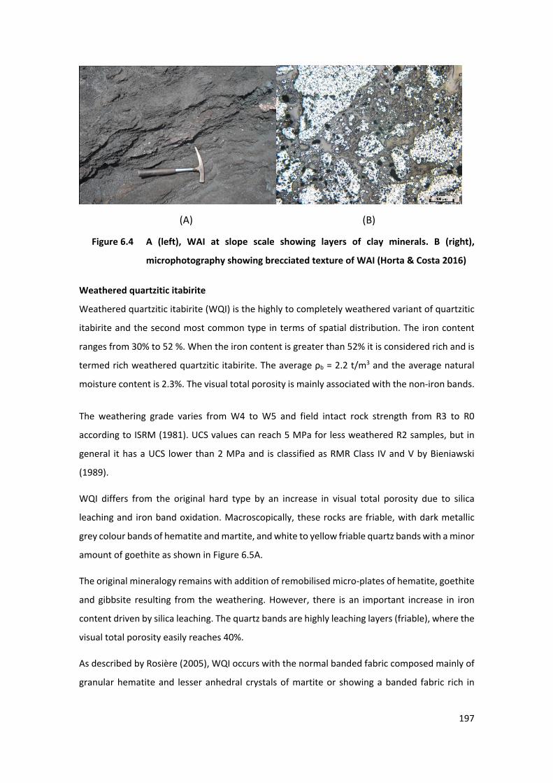
197
(A) (B)
54 Figure 6.4 A (left), WAI at slope scale showing layers of clay minerals. B (right),
microphotography showing brecciated texture of WAI (Horta & Costa 2016)
Weathered quartzitic itabirite
Weathered quartzitic itabirite (WQI) is the highly to completely weathered variant of quartzitic
itabirite and the second most common type in terms of spatial distribution. The iron content
ranges from 30% to 52 %. When the iron content is greater than 52% it is considered rich and is
termed rich weathered quartzitic itabirite. The average ρb = 2.2 t/m3 and the average natural
moisture content is 2.3%. The visual total porosity is mainly associated with the non-iron bands.
The weathering grade varies from W4 to W5 and field intact rock strength from R3 to R0
according to ISRM (1981). UCS values can reach 5 MPa for less weathered R2 samples, but in
general it has a UCS lower than 2 MPa and is classified as RMR Class IV and V by Bieniawski
(1989).
WQI differs from the original hard type by an increase in visual total porosity due to silica
leaching and iron band oxidation. Macroscopically, these rocks are friable, with dark metallic
grey colour bands of hematite and martite, and white to yellow friable quartz bands with a minor
amount of goethite as shown in Figure 6.5A.
The original mineralogy remains with addition of remobilised micro-plates of hematite, goethite
and gibbsite resulting from the weathering. However, there is an important increase in iron
content driven by silica leaching. The quartz bands are highly leaching layers (friable), where the
visual total porosity easily reaches 40%.
As described by Rosière (2005), WQI occurs with the normal banded fabric composed mainly of
granular hematite and lesser anhedral crystals of martite or showing a banded fabric rich in
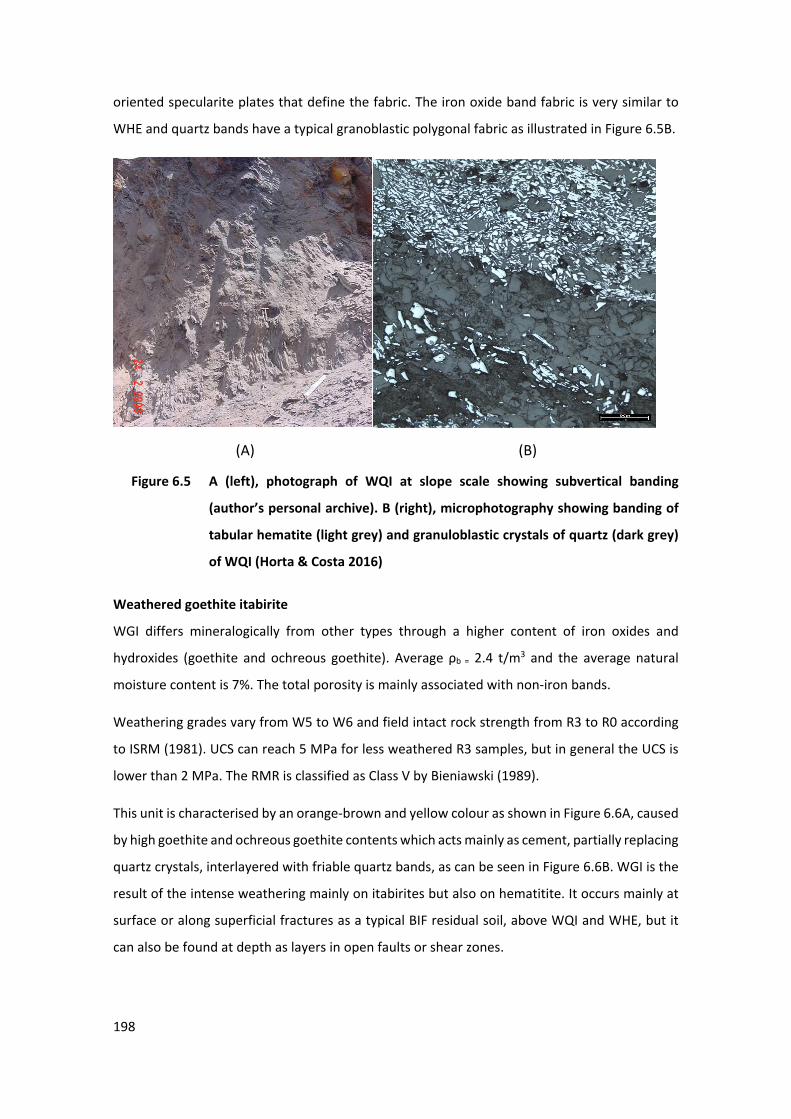
198
oriented specularite plates that define the fabric. The iron oxide band fabric is very similar to
WHE and quartz bands have a typical granoblastic polygonal fabric as illustrated in Figure 6.5B.
(A) (B)
55 Figure 6.5 A (left), photograph of WQI at slope scale showing subvertical banding
(author’s personal archive). B (right), microphotography showing banding of
tabular hematite (light grey) and granuloblastic crystals of quartz (dark grey)
of WQI (Horta & Costa 2016)
Weathered goethite itabirite
WGI differs mineralogically from other types through a higher content of iron oxides and
hydroxides (goethite and ochreous goethite). Average ρb = 2.4 t/m3 and the average natural
moisture content is 7%. The total porosity is mainly associated with non-iron bands.
Weathering grades vary from W5 to W6 and field intact rock strength from R3 to R0 according
to ISRM (1981). UCS can reach 5 MPa for less weathered R3 samples, but in general the UCS is
lower than 2 MPa. The RMR is classified as Class V by Bieniawski (1989).
This unit is characterised by an orange-brown and yellow colour as shown in Figure 6.6A, caused
by high goethite and ochreous goethite contents which acts mainly as cement, partially replacing
quartz crystals, interlayered with friable quartz bands, as can be seen in Figure 6.6B. WGI is the
result of the intense weathering mainly on itabirites but also on hematitite. It occurs mainly at
surface or along superficial fractures as a typical BIF residual soil, above WQI and WHE, but it
can also be found at depth as layers in open faults or shear zones.
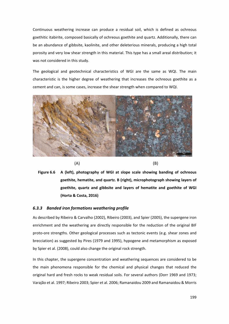
199
Continuous weathering increase can produce a residual soil, which is defined as ochreous
goethitic itabirite, composed basically of ochreous goethite and quartz. Additionally, there can
be an abundance of gibbsite, kaolinite, and other deleterious minerals, producing a high total
porosity and very low shear strength in this material. This type has a small areal distribution; it
was not considered in this study.
The geological and geotechnical characteristics of WGI are the same as WQI. The main
characteristic is the higher degree of weathering that increases the ochreous goethite as a
cement and can, is some cases, increase the shear strength when compared to WQI.
(A) (B)
56 Figure 6.6 A (left), photography of WGI at slope scale showing banding of ochreous
goethite, hematite, and quartz. B (right), microphotograph showing layers of
goethite, quartz and gibbsite and layers of hematite and goethite of WGI
(Horta & Costa, 2016)
6.3.3 Banded iron formations weathering profile
As described by Ribeiro & Carvalho (2002), Ribeiro (2003), and Spier (2005), the supergene iron
enrichment and the weathering are directly responsible for the reduction of the original BIF
proto-ore strengths. Other geological processes such as tectonic events (e.g. shear zones and
brecciation) as suggested by Pires (1979 and 1995), hypogene and metamorphism as exposed
by Spier et al. (2008), could also change the original rock strength.
In this chapter, the supergene concentration and weathering sequences are considered to be
the main phenomena responsible for the chemical and physical changes that reduced the
original hard and fresh rocks to weak residual soils. For several authors (Dorr 1969 and 1973;
Varajão et al. 1997; Ribeiro 2003; Spier et al. 2006; Ramanaidou 2009 and Ramanaidou & Morris
200
2010) the original high-strength rocks (proto rock) were affected by weathering resulting in a
partial or complete mineral leaching, and chemical alteration.
Evaluating the canga origin, Spier et al. (2019) proposes a genetic and evolution model of the
weathering profile for itabirites of the Iron Quadrangle that includes a sequence of chemical
weathering and pedogenic processes. This model allows an independence of the pedolith
(ferruginous duricrusts) and saprolite (supergene iron ore) formation processes and the
evolution of the weathering profiles developed in itabirite. It also indicates less effective
weathering in the quartz itabirite than in the dolomitic itabirite, resulting in smaller ore bodies,
but with the same geochemical trends.
As presented by Ramanaidou and Morris (2010), the supergene iron enrichment and subsequent
strength reduction can be divided into two main processes:
• The supergene mimetic mechanism, which occurs below the watertable Morris (1980,
2002, 2002a and 2003) and the association with presence of structures, topography
and climate. It is also responsible for producing deep and large iron-rich deposits.
• The supergene lateritic weathering, which is the result of ganga mineral dissolution
and iron reconcentration above the watertable. This process produces several
weathering profiles characterised by different relative iron enrichment and ganga
mineral composition.
Studies by Ramanaidou (1989), Ribeiro and Carvalho (2002), Ribeiro (2003) and Ramanaidou
(2009) suggest that during the first leaching processes there were no volumetric changes in the
quartz to goethite substitution. Progressively, when gangue minerals start to be leached
volumetric changes take place (more effective on dolomites, but also in quartz bands) and the
replacement of quartz to goethite increases porosity. In cases where this porosity was
completely cemented by goethite or iron hydroxide at superficial levels, a hard crust called canga
was created.
As presented by Spier et al. (2003), superficial water is the main physical and chemical agent
responsible for the effective dissolution and leaching of carbonates and siliceous minerals, and
for the oxidation and hydration of iron-based minerals. The BIF form an important granular
aquifer (especially in the weathered zones), with high secondary porosity and storability that
reduces with depth, and the aquifer morphology is highly influenced by the structural domain
and fracture distribution.
201
As proposed by Dorr (1969), due to the efficiency of the weathering in tropical climates induced
by high pluviometric index (rainfall), the high primary and secondary permeability of BIF rocks,
favourable topography, seasonal climate temperature changes, and physical/chemical reactions
lead to a weathering profile that can often extend to 200 m and even reach over 400 m in depth.
In addition, synclinal and anticlinal geological features, together with the presence of favourable
subvertical structural controls, as defined by high banding angles and extensional fractures,
facilitated superficial and groundwater penetration and circulation, supporting the effectiveness
of the weathering. Thus, considering the weak rocks associated with these deep weathering
profiles, found at or close to the surface, may range from highly weathered rock to residual soil.
Consequently, the strength of the weathered material might vary due to original proto-lithology
differences, mainly mineralogy, in the original three compositional types of fresh BIF, as
described by Dorr (1969), weathering intensity and geological features (such as fold or faults),
and all this geological information must be considered when evaluating strength characteristics
and behaviour.
It is also recognised that original anisotropy of some lithotypes (induced by compositional
metamorphic banding or foliation) represents an extra complexity for weathering profile
delimitation, mainly due to lateral physical and chemical variations along and through the
banding. This feature can cause strength and lateral permeability variations at the same depth
in the weathering profile, making anisotropy an important characteristic to be considered. All of
this reinforces the idea that a more pragmatic geological approach is required to define
geomechanical or lithotypes domains.
Mineral changes are not the only noted effect of the weathering. Porosity increase is also
recognised as an important change seen in those rocks. Studies by Morris (2002 and 2002a) and
Taylor et al. (2001) argue that the supergene process can reduce the thickness of the BIF by 32%
to 40% and increase total porosity from 6% to 30% (Mourão 2007). Based on that, weathering
produces an effective softening from the leaching, and the remaining iron oxide bands have a
high void ratio that could be cemented by secondary iron oxides (recrystallised hematite or
goethite). This material exhibits weak strength, and the iron enrichment promotes an increase
in bulk density due to new iron mineral concentrations and non-iron mineral leaching.
The latter finding agrees with Aylmer et al. (1978), when evaluating bulk density, iron grade, and
total porosity for Mount Tom Price iron ore, concluding that iron grade and bulk density presents
good correlation. However, accuracy is primarily affected by high values and a variability of total
porosity. According to Box & Reid (1976), for iron ore formation from Cockatoo Island, true
202
specific gravity could be expressed as a function of iron content. However, due to the complexity
and multiple factors involved, the same could not be proven for porosity. Thomson (1963),
concludes that, for iron ore samples from Australia, a theoretical hematite-quartz curve can be
used for bulk density definition and can allow an approximate iron content calculation. The same
was found for South African iron ore as presented by Nel (2007), which established for the Sishen
deposits, that porosity is directly correlated to dry and bulk density, providing a reliable
calculation index.
For Brazilian iron ore mines, studies by Ribeiro et al. (2014); Santos (2007) and Santos et al.
(2005) have evaluated the association between bulk density and iron content for Vale Iron
Quadrangle BIF and concluded that there is a positive linear correlation between the total iron
content and the bulk density. In addition, those authors argue that the weathering has an
important influence on the bulk density and iron content dispersion imposed by the total
porosity.
6.4 SATURATED AND UNSATURATED APPROACHES BRIEF LITERATURE REVIEW
6.4.1 Industry overview
Brazilian iron ore mines are exposed to cyclic hydrogeological conditions that have ranged from
almost fully saturated conditions that existed before mining began to near fully depressurised
conditions during mining that have resulted in substantial reduction in groundwater levels.
Additionally, Brazil’s seasonal rainy and dry seasons can induce water level variations that can
reach a dozen metres during a single hydrological cycle considered not large give weathering
profile that can reach 400 metres depth. This cyclical watertable charge and discharge (long and
short-term) will impose alternating saturated and unsaturated conditions to the highly
weathered BIF and therefore understanding the resulting changes posed by this variation in
shear strength is the focus of this section.
The Iron Quadrangle general annual pluviometry varies between 1,500 mm to 1,700 mm with
approximately 90% of annual precipitation concentrated during October to March (summer).
During this high rainfall period it has been identified that superficial aquifers (or transient
aquifers) can form, which are intimately associated with the seasonality fluctuation. These
typically vary in depth from 1 m to 10 m depending on different variables (Reboita et al. 2015).
The deep aquifer, however, is generally only minimally affected by the climate’s seasonality but
is strongly influenced by mine dewatering.
203
Concerning the BIF hydrogeological characteristics, the WHE, WQI, and WGI behave as granular
aquifers with high porosity and storage coefficients. However, due to the relatively higher
percentage of clay minerals WAI behaves as an aquitard and can locally modify the aquifer flow
or generate confined aquifers (Ventura 2009).
The development of unsaturated soil mechanics theory has principally taken place in the civil-
geotechnical engineering field (Fredlund et al. 1978). Consequently, up until recent times most
applications of unsaturated soil mechanics theory in the field of civil slope stability have been
limited to relatively shallow (in mining terms), well instrumented and monitored excavations. In
addition, as this field is relatively young in Brazil, few mining engineers have been educated in
this theory and been confident in applying it to mining engineering designs. For this reason, few
commercial laboratories offer unsaturated soil testing and main development came from
academic researches.
In situ testing in unsaturated soils could not be disregarded, however there are no proven
methods of investigations for cone penetration, pressure meters, or standard penetration test
for these types of soils similar to BIF as presented by Miller el al (2015).
For decades, slope stability analyses in weathered and weak BIF (with soil behaviour) were based
on a saturated approach using effective stress parameters. The idea of using unsaturated
concepts in the analyses is more recent and considers the pore air and water pressures existing
in the voids near surface, above the water level. In regard to weathered BIF, there has been an
industry concern that due to the typical high void content and high permeability of the materials
the amount of matric suction that could develop would be relatively low and easily lost.
However, even a minor presence of clay minerals and silt content can change these
characteristics, thereby inducing sufficient negative pore pressures that are able to influence
slope stability, as presented by Lu and Likos (2004) and Likos et al. (2010) who argue that matric
suction contributes to cohesion and increases shear strength of unsaturated soils. Also, studies
of iron formations by Grgic et al. (2005) suggested that an improvement on strength and
cohesion of unsaturated oolithic iron ore can occur due to the negative porewater pressure
effects.
In current Brazilian iron mining operations, the incomprehension of unsaturated material
behaviour and the absence of unsaturated parameters able to evaluate negative pore pressure
effects (suction) above the watertable for temporary and or permanent, has forced the
geotechnical mining engineers to adjust the unsaturated field conditions to saturated
parameters adopting effective results for this condition. With this approach, it has been possible
204
to estimate possible suction effects on slope stability analyses. This incorrect approach can be
easily replaced by unsaturated laboratory tests able to properly define the material water
content (saturation) and porewater content (pore pressure) above the watertable that could
define for some completely weathered BIF negative porewater content (suction) able to add an
apparent cohesion on slope stability analyses.
The importance of evaluating the unsaturated soil characteristics has been primary noted by
researchers undertaken outside the mining industry where the shear strength of soils and
residual soils with negative porewater pressure can increase the stability of slopes, especially
those having shallow but steep surfaces, as supported by Fredlund et al. (1978). So far, matric
suction effects have rarely been considered in Brazilian open pit slope stability evaluations, so
design parameters and effective stress parameters have been obtained through conventional
saturated laboratory testing. This latter approach seems to be adequate for high rainfall areas,
where long-term slope stability is required and soil materials with high permeability and not
suitable to seasonal water changes. However, it tends to be too conservative when applied for
short-term slopes above the water level. The use of unsaturated soil mechanics is therefore an
opportunity to correct the balance between safety and economical slope design.
For Brazilian iron ore mines, regarding the application of the unsaturated theory to mining
geotechnical engineering, there has been a delay in both the transfer and application of
knowledge from the civil to the mining fields with several significant challenges presenting
themselves in larger-scale mining applications, which include:
• The increasing scale, height and variability of mining slopes.
• The difficulty and cost of instrumenting large and high slopes particularly regarding
measuring in situ matric suction.
• The exposure of the slopes to the climatic variability and inability to control matric
suctions (e.g. preventing the ingress of water).
• The fact that most soil is highly to completely weathered rocks that contain complex
relic structures.
• Unlike shallow slopes, confining stress affects the unsaturated characteristics of samples
(there is a considerably higher range of confining stresses experienced in larger slopes).
• Difficulty to find commercial laboratories able to undertake appropriate matric suction
tests.
Despite these challenges, consideration has been given to using unsaturated soil mechanics
theory for open pit iron ore mines. Grgic et al. (2005) proposed for France iron ore deposits a
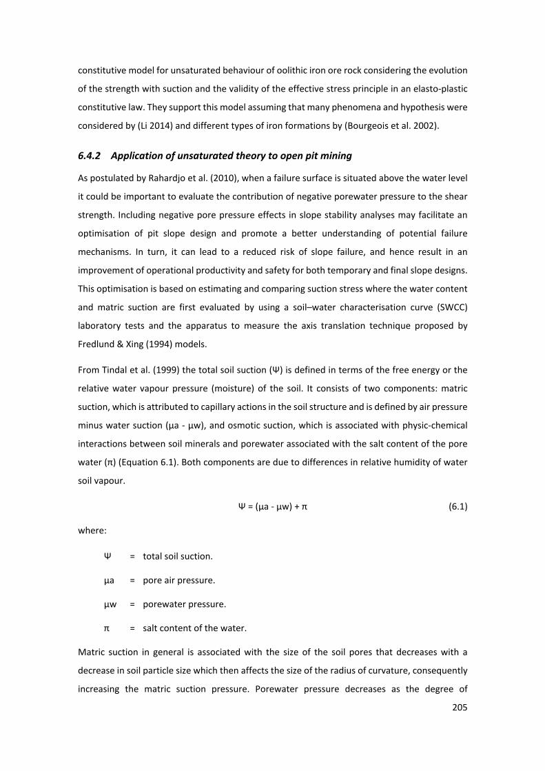
205
constitutive model for unsaturated behaviour of oolithic iron ore rock considering the evolution
of the strength with suction and the validity of the effective stress principle in an elasto-plastic
constitutive law. They support this model assuming that many phenomena and hypothesis were
considered by (Li 2014) and different types of iron formations by (Bourgeois et al. 2002).
6.4.2 Application of unsaturated theory to open pit mining
As postulated by Rahardjo et al. (2010), when a failure surface is situated above the water level
it could be important to evaluate the contribution of negative porewater pressure to the shear
strength. Including negative pore pressure effects in slope stability analyses may facilitate an
optimisation of pit slope design and promote a better understanding of potential failure
mechanisms. In turn, it can lead to a reduced risk of slope failure, and hence result in an
improvement of operational productivity and safety for both temporary and final slope designs.
This optimisation is based on estimating and comparing suction stress where the water content
and matric suction are first evaluated by using a soil–water characterisation curve (SWCC)
laboratory tests and the apparatus to measure the axis translation technique proposed by
Fredlund & Xing (1994) models.
From Tindal et al. (1999) the total soil suction (Ψ) is defined in terms of the free energy or the
relative water vapour pressure (moisture) of the soil. It consists of two components: matric
suction, which is attributed to capillary actions in the soil structure and is defined by air pressure
minus water suction (μa - μw), and osmotic suction, which is associated with physic-chemical
interactions between soil minerals and porewater associated with the salt content of the pore
water (π) (Equation 6.1). Both components are due to differences in relative humidity of water
soil vapour.
Ψ = (μa - μw) + π (6.1)
where:
Ψ = total soil suction.
μa = pore air pressure.
μw = porewater pressure.
π = salt content of the water.
Matric suction in general is associated with the size of the soil pores that decreases with a
decrease in soil particle size which then affects the size of the radius of curvature, consequently
increasing the matric suction pressure. Porewater pressure decreases as the degree of
206
saturation decreases. For osmotic suction, the presence of dissolved salts in water decreases
the soil–water pressures, which then increases the osmotic suction.
Unsaturated soils behaviour is controlled by total suction, ψ that in turn is composed of matric
and osmotic suction. However, authors such as Fredlund et al. (2012) and Lu and Likos (2004)
have suggested that osmotic suction be ignored for low salinity engineering applications and
according to Nishimura et al. (1999) matric suction is of primary interest for engineering
problems involving unsaturated soils. This suggestion is supported for BIF due to the low salinity
normally observed at iron ore aquifers (13.2 μs/cm) as defined by Mourão, 2007 for Cauê
formation, host of iron ore mines. Thus, for Brazilian iron ore deposits negative pore pressures
should be defined by evaluating only the matric suction.
For indirect determination of the porewater pressures, Vanapalli et al. (1996) and Vanapalli &
Fredlund (2000) have proposed techniques that correlate unsaturated shear strength to
saturated shear strength, and that the SWCC describes the amount of water retained in a soil
(expressed as mass or volume water content) when it is in equilibrium at a given matric
potential. The SWCC is an important hydraulic property related to size and connectivity of pore
spaces and is therefore strongly affected by soil texture and structure. The curve is plotted on a
logarithmic scale and is highly nonlinear due to the matric potential extending over several
orders of magnitude for the range of water contents. Typical curves represent different soil
specimens (textures), demonstrating the effects of porosity (saturated water content) resulting
from variable pore size distributions (Perucho et al. 2014).
For an unsaturated soil, the matric suction and unsaturated friction angle (ɸb) are additional
parameters that increase the shear strength compared with saturated shear strength. The shear
strength of an unsaturated soil as a function of ψ can be estimated experimentally. The effective
friction angle (ɸ’) and effective cohesion (c’) as the intercept of the ‘extended’ Mohr–Coulomb
(MC) failure envelope in the shear stress axis when the net normal stress and the matric suction
at failure are equal to zero and are determined by conventional direct shear or triaxial tests on
saturated soil specimens. The slope of shearing resistance with respect to ψ is defined by the ɸb
which can assumed to be either linear, bilinear of nonlinear.
The air entry value (AEV), point ‘A’ in Figure 6.7, is defined in Fredlund & Rahardjo (1993) as the
matric suction value that must be exceeded before air is drawn into the soil pores. In terms of
strength, it is the point at which the strength of the soil deviates from its saturated effective MC
behaviour. If matric suction exceeds the AEV, the strength is assumed to follow a linear envelope
with ɸb ≈ ɸ' used for positive pore pressures. Considering changes observed above the AEV
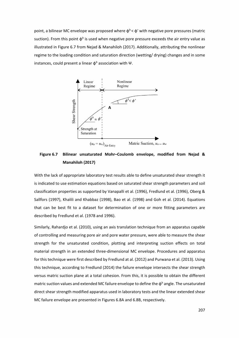
207
point, a bilinear MC envelope was proposed where ɸb < ɸ' with negative pore pressures (matric
suction). From this point ɸb is used when negative pore pressure exceeds the air entry value as
illustrated in Figure 6.7 from Nejad & Manahiloh (2017). Additionally, attributing the nonlinear
regime to the loading condition and saturation direction (wetting/ drying) changes and in some
instances, could present a linear ɸb association with Ψ.
57 Figure 6.7 Bilinear unsaturated Mohr–Coulomb envelope, modified from Nejad &
Manahiloh (2017)
With the lack of appropriate laboratory test results able to define unsaturated shear strength it
is indicated to use estimation equations based on saturated shear strength parameters and soil
classification properties as supported by Vanapalli et al. (1996), Fredlund et al. (1996), Oberg &
Sallfors (1997), Khalili and Khabbaz (1998), Bao et al. (1998) and Goh et al. (2014). Equations
that can be best fit to a dataset for determination of one or more fitting parameters are
described by Fredlund et al. (1978 and 1996).
Similarly, Rahardjo et al. (2010), using an axis translation technique from an apparatus capable
of controlling and measuring pore air and pore water pressure, were able to measure the shear
strength for the unsaturated condition, plotting and interpreting suction effects on total
material strength in an extended three-dimensional MC envelope. Procedures and apparatus
for this technique were first described by Fredlund at al. (2012) and Purwana et al. (2013). Using
this technique, according to Fredlund (2014) the failure envelope intersects the shear strength
versus matric suction plane at a total cohesion. From this, it is possible to obtain the different
matric suction values and extended MC failure envelope to define the ɸb angle. The unsaturated
direct shear strength modified apparatus used in laboratory tests and the linear extended shear
MC failure envelope are presented in Figures 6.8A and 6.8B, respectively.
A
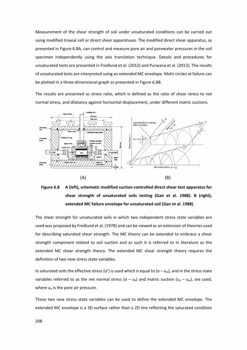
208
Measurement of the shear strength of soil under unsaturated conditions can be carried out
using modified triaxial cell or direct shear apparatuses. The modified direct shear apparatus, as
presented in Figure 6.8A, can control and measure pore air and porewater pressures in the soil
specimen independently using the axis translation technique. Details and procedures for
unsaturated tests are presented in Fredlund et al. (2012) and Purwana et al. (2013). The results
of unsaturated tests are interpreted using an extended MC envelope. Mohr circles at failure can
be plotted in a three-dimensional graph as presented in Figure 6.8B.
The results are presented as stress ratio, which is defined as the ratio of shear stress to net
normal stress, and dilatancy against horizontal displacement, under different matric suctions.
(A) (B)
58 Figure 6.8 A (left), schematic modified suction controlled direct shear test apparatus for
shear strength of unsaturated soils testing (Gan et al. 1988). B (right),
extended MC failure envelope for unsaturated soil (Gan et al. 1988)
The shear strength for unsaturated soils in which two independent stress state variables are
used was proposed by Fredlund et al. (1978) and can be viewed as an extension of theories used
for describing saturated shear strength. The MC theory can be extended to embrace a shear
strength component related to soil suction and as such it is referred to in literature as the
extended MC shear strength theory. The extended MC shear strength theory requires the
definition of two new stress state variables.
In saturated soils the effective stress (σ’) is used which is equal to (σ – uw), and in the stress state
variables referred to as the net normal stress (σ – ua) and matric suction (ua – uw), are used,
where ua is the pore air pressure.
These two new stress state variables can be used to define the extended MC envelope. The
extended MC envelope is a 3D surface rather than a 2D line reflecting the saturated condition
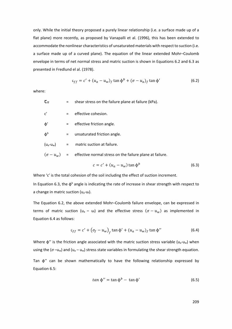
209
only. While the initial theory proposed a purely linear relationship (i.e. a surface made up of a
flat plane) more recently, as proposed by Vanapalli et al. (1996), this has been extended to
accommodate the nonlinear characteristics of unsaturated materials with respect to suction (i.e.
a surface made up of a curved plane). The equation of the linear extended Mohr–Coulomb
envelope in terms of net normal stress and matric suction is shown in Equations 6.2 and 6.3 as
presented in Fredlund el al. (1978).
ꞇ𝑓𝑓𝑓𝑓 = 𝑅𝑅′ + (𝑢𝑢𝑎𝑎 − 𝑢𝑢𝑤𝑤)𝑓𝑓 tanɸ𝑏𝑏 + (𝜎𝜎 − 𝑢𝑢𝑎𝑎)𝑓𝑓 tanɸ′ (6.2)
where:
ꞇff = shear stress on the failure plane at failure (kPa).
c’ = effective cohesion.
ɸ’ = effective friction angle.
ɸb = unsaturated friction angle.
(ua-uw) = matric suction at failure.
(𝜎𝜎 − 𝑢𝑢𝑤𝑤) = effective normal stress on the failure plane at failure.
𝑅𝑅 = 𝑅𝑅′ + (𝑢𝑢𝑎𝑎 − 𝑢𝑢𝑤𝑤) tanɸ𝑏𝑏 (6.3)
Where ‘c’ is the total cohesion of the soil including the effect of suction increment.
In Equation 6.3, the ɸb angle is indicating the rate of increase in shear strength with respect to
a change in matric suction (ua-uf).
The Equation 6.2, the above extended Mohr–Coulomb failure envelope, can be expressed in
terms of matric suction (ua – uf) and the effective stress (𝜎𝜎 − 𝑢𝑢𝑤𝑤) as implemented in
Equation 6.4 as follows:
ꞇ𝑓𝑓𝑓𝑓 = 𝑅𝑅′ + �𝜎𝜎𝑓𝑓 − 𝑢𝑢𝑤𝑤�𝑓𝑓 tanɸ′ + (𝑢𝑢𝑎𝑎 − 𝑢𝑢𝑤𝑤)𝑓𝑓 tanɸ′′ (6.4)
Where ɸ’’ is the friction angle associated with the matric suction stress variable (ua-uw) when
using the (𝜎𝜎 –uw) and (ua – uw) stress state variables in formulating the shear strength equation.
Tan ɸ’’ can be shown mathematically to have the following relationship expressed by
Equation 6.5:
𝑡𝑡𝑡𝑡𝑡𝑡 ɸ′′ = tanɸ𝑏𝑏 − tanɸ′ (6.5)
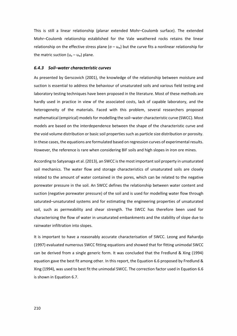
210
This is still a linear relationship (planar extended Mohr–Coulomb surface). The extended
Mohr–Coulomb relationship established for the Vale weathered rocks retains the linear
relationship on the effective stress plane (σ – uw) but the curve fits a nonlinear relationship for
the matric suction (ua – uw) plane.
6.4.3 Soil–water characteristic curves
As presented by Gerscovich (2001), the knowledge of the relationship between moisture and
suction is essential to address the behaviour of unsaturated soils and various field testing and
laboratory testing techniques have been proposed in the literature. Most of these methods are
hardly used in practice in view of the associated costs, lack of capable laboratory, and the
heterogeneity of the materials. Faced with this problem, several researchers proposed
mathematical (empirical) models for modelling the soil–water characteristic curve (SWCC). Most
models are based on the interdependence between the shape of the characteristic curve and
the void volume distribution or basic soil properties such as particle size distribution or porosity.
In these cases, the equations are formulated based on regression curves of experimental results.
However, the reference is rare when considering BIF soils and high slopes in iron ore mines.
According to Satyanaga et al. (2013), an SWCC is the most important soil property in unsaturated
soil mechanics. The water flow and storage characteristics of unsaturated soils are closely
related to the amount of water contained in the pores, which can be related to the negative
porewater pressure in the soil. An SWCC defines the relationship between water content and
suction (negative porewater pressure) of the soil and is used for modelling water flow through
saturated–unsaturated systems and for estimating the engineering properties of unsaturated
soil, such as permeability and shear strength. The SWCC has therefore been used for
characterising the flow of water in unsaturated embankments and the stability of slope due to
rainwater infiltration into slopes.
It is important to have a reasonably accurate characterisation of SWCC. Leong and Rahardjo
(1997) evaluated numerous SWCC fitting equations and showed that for fitting unimodal SWCC
can be derived from a single generic form. It was concluded that the Fredlund & Xing (1994)
equation gave the best fit among other. In this report, the Equation 6.6 proposed by Fredlund &
Xing (1994), was used to best fit the unimodal SWCC. The correction factor used in Equation 6.6
is shown in Equation 6.7.
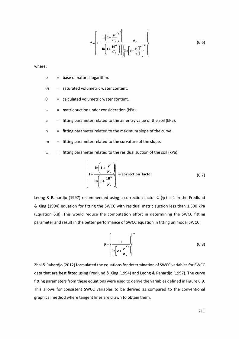
211
(6.6)
where:
e = base of natural logarithm.
θs = saturated volumetric water content.
θ = calculated volumetric water content.
ψ = matric suction under consideration (kPa).
a = fitting parameter related to the air entry value of the soil (kPa).
n = fitting parameter related to the maximum slope of the curve.
m = fitting parameter related to the curvature of the slope.
ψr = fitting parameter related to the residual suction of the soil (kPa).
(6.7)
Leong & Rahardjo (1997) recommended using a correction factor C (ψ) = 1 in the Fredlund
& Xing (1994) equation for fitting the SWCC with residual matric suction less than 1,500 kPa
(Equation 6.8). This would reduce the computation effort in determining the SWCC fitting
parameter and result in the better performance of SWCC equation in fitting unimodal SWCC.
(6.8)
Zhai & Rahardjo (2012) formulated the equations for determination of SWCC variables for SWCC
data that are best fitted using Fredlund & Xing (1994) and Leong & Rahardjo (1997). The curve
fitting parameters from these equations were used to derive the variables defined in Figure 6.9.
This allows for consistent SWCC variables to be derived as compared to the conventional
graphical method where tangent lines are drawn to obtain them.
+
+
+
−=mn
s
r
r
aeC
C
ψ
θψ
θ
ln101ln
1ln1
6
factor correction101ln
1ln1
6=
+
+
−
r
r
ψ
ψψ
m
n
ae
+
=ψ
θ
ln
1
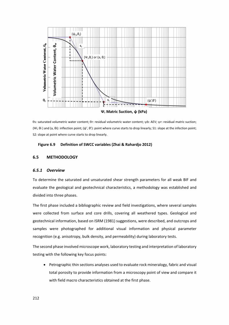
212
θs: saturated volumetric water content; θr: residual volumetric water content; ψb: AEV; ψr: residual matric suction;
(Ψi, θi ) and (a, θi): inflection point; (ψ’, θ’): point where curve starts to drop linearly; S1: slope at the infection point;
S2: slope at point where curve starts to drop linearly.
59 Figure 6.9 Definition of SWCC variables (Zhai & Rahardjo 2012)
6.5 METHODOLOGY
6.5.1 Overview
To determine the saturated and unsaturated shear strength parameters for all weak BIF and
evaluate the geological and geotechnical characteristics, a methodology was established and
divided into three phases.
The first phase included a bibliographic review and field investigations, where several samples
were collected from surface and core drills, covering all weathered types. Geological and
geotechnical information, based on ISRM (1981) suggestions, were described, and outcrops and
samples were photographed for additional visual information and physical parameter
recognition (e.g. anisotropy, bulk density, and permeability) during laboratory tests.
The second phase involved microscope work, laboratory testing and interpretation of laboratory
testing with the following key focus points:
• Petrographic thin sections analyses used to evaluate rock mineralogy, fabric and visual
total porosity to provide information from a microscopy point of view and compare it
with field macro characteristics obtained at the first phase.
Ψr Matric Suction, ψ (kPa)
Volu
met
ric W
ater
Con
tent
, θw
213
• Laboratory tests which included determination of in situ and laboratory permeability,
natural moisture content, saturated and unsaturated shear strength parameters,
porewater pressure, and soil–water characteristic curves to evaluate unsaturated
behaviour.
• UCS parameters were determined using RocData 5.0 (Rocscience 2021) adjusted fitted
curves used to determine the anisotropic ratio.
• Geotechnical characterisation using Unified Soil Classification System (USCS) soil
classification, bulk density, particle size distributions, and Atterberg limits to provide
bases for geomechanical behaviour determination and support a correlation between
geological characteristics and geotechnical parameters of each material.
The third phase consisted of interpreting the dataset derived from the previous phases
proposing correlations involving physical characteristics, geotechnical parameters and
geomechanical behaviour of each material type. It also included writing this manuscript.
Special attention was given to investigate anisotropic effects on geotechnical behaviour for
saturated and unsaturated conditions, and total and effective shear parameters. This involved
the use of single stage saturated direct shear tests with free drainage (IDST), single stage
unsaturated direct shear tests with matric suction measurements (UIDST), consolidated
undrained triaxial tests (CIU) parallel and perpendicular to banding, and soil–water
characteristic curve (SWCC) determination with wetting and drying curves.
As usual in soil tests, large variations in values of rock sample strength were obtained, and these
could often be attributed to e.g. sampling errors, the accuracy of sample preparation, testing
procedures and incorrect geological sample identification. To reduce variability due to geological
effects and defects a sampling validation approach presented in Appendix I was used. This
procedure involves a sample grouping to reduce the variance and provide a better lithotype
characterisation.
This approach checks the samples before carrying out the tests, as follows:
• Samples were grouped based on core logging or superficial mapping defined by the
level of weathering based on the ISRM (1981) table, geological characteristics (e.g.
banding features), transverse isotropy direction (β angle) and ρb.
• Geological features such as intense folding, presence of specularite, infill material with
a different weathered degree, quartz or calcite veins and others that do not represent
typical itabirite heterogeneity was discarded.
214
• Itabirite samples that did not have the typical visible compositional metamorphic
banding (heterogeneity) were not evaluated to avoid the scale effect represented by
different thickness of banding layers.
• Extreme outlier results were removed according to the box plot statistical
methodology (Whitaker et al. 2013). This technique identifies the mild outlier’s values
from the quartiles (Qt) determination, based on the Equation 6.9.
Values below the lower inner fence (QtLower):
QtLower = 1Qt - 1.5(3Qt - 1Qt) (6.9)
and values above the upper inner fence (Qtupper) as Equation 6.10:
Qtupper = 3Qt + 1.5(3Qt - 1Qt) (6.10)
where 1Qt is the first quartile and 3Qt is the third quartile.
The 3Qt evaluates database dispersion around a central data leaving 75% of data below
the sum and is defined by Equation 6.11:
3Qt = × + 1.5.IQR (6.11)
The first or inferior quartile (1Qt) evaluates database dispersion around a central data
leaving 25% of data below the sum and is defined by the Equation 6.12.
1Qt = × - 1.5.IQR (6.12)
Interquartile ranges (IQR) measure how spread out from a central data the values are
and these form what are called outliers and are defined by Equation 6.13:
IQR = 3Qt - 1Qt (6.13)
The first or inferior quartile (1Qt) evaluates database dispersion around a central data
leaving 25% of data below the sum and is defined by the Equation 6.14.
1Qt = × - 1.5.IQR (6.14)
Interquartile ranges (IQR) measure how spread out from a central data the values are
and these forms what are called outliers and are defined by Equation 6.15:
IQR = 3Qt - 1Qt (6.15)
In cases of reduced number of test results (around 10), the arithmetic mean (mean) was used
to determine material property average values.
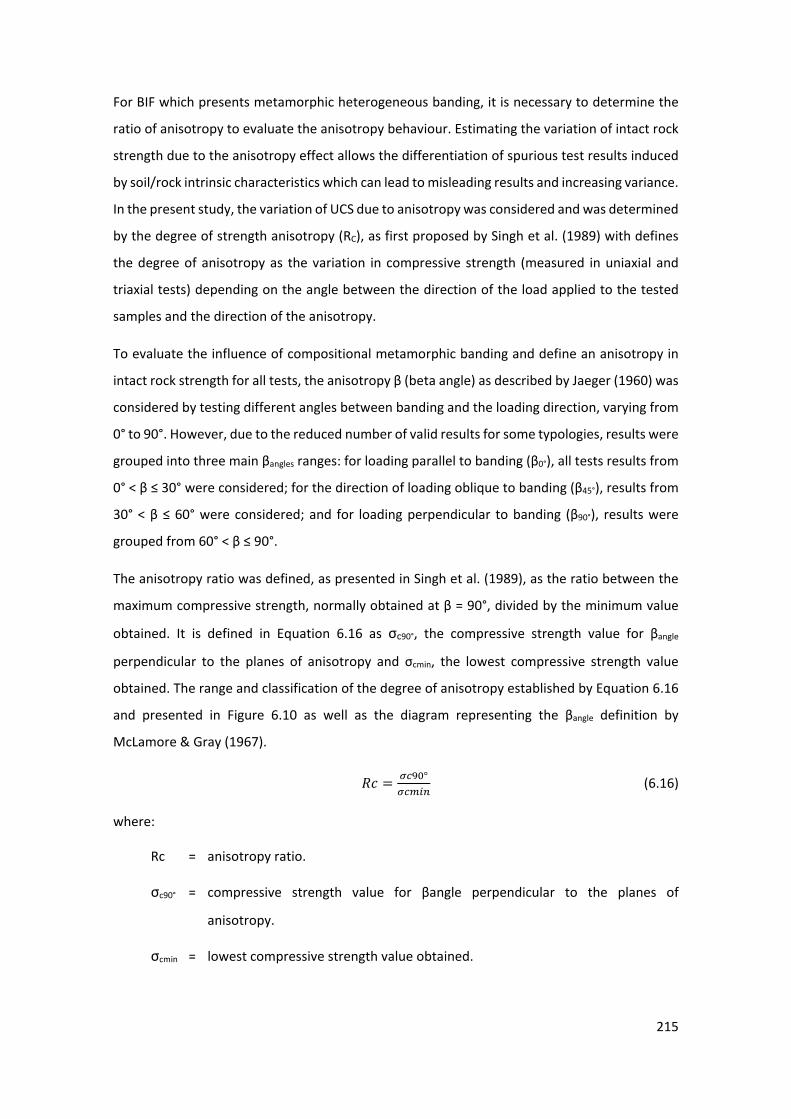
215
For BIF which presents metamorphic heterogeneous banding, it is necessary to determine the
ratio of anisotropy to evaluate the anisotropy behaviour. Estimating the variation of intact rock
strength due to the anisotropy effect allows the differentiation of spurious test results induced
by soil/rock intrinsic characteristics which can lead to misleading results and increasing variance.
In the present study, the variation of UCS due to anisotropy was considered and was determined
by the degree of strength anisotropy (RC), as first proposed by Singh et al. (1989) with defines
the degree of anisotropy as the variation in compressive strength (measured in uniaxial and
triaxial tests) depending on the angle between the direction of the load applied to the tested
samples and the direction of the anisotropy.
To evaluate the influence of compositional metamorphic banding and define an anisotropy in
intact rock strength for all tests, the anisotropy β (beta angle) as described by Jaeger (1960) was
considered by testing different angles between banding and the loading direction, varying from
0° to 90°. However, due to the reduced number of valid results for some typologies, results were
grouped into three main βangles ranges: for loading parallel to banding (β0°), all tests results from
0° < β ≤ 30° were considered; for the direction of loading oblique to banding (β45°), results from
30° < β ≤ 60° were considered; and for loading perpendicular to banding (β90°), results were
grouped from 60° < β ≤ 90°.
The anisotropy ratio was defined, as presented in Singh et al. (1989), as the ratio between the
maximum compressive strength, normally obtained at β = 90°, divided by the minimum value
obtained. It is defined in Equation 6.16 as σc90°, the compressive strength value for βangle
perpendicular to the planes of anisotropy and σcmin, the lowest compressive strength value
obtained. The range and classification of the degree of anisotropy established by Equation 6.16
and presented in Figure 6.10 as well as the diagram representing the βangle definition by
McLamore & Gray (1967).
𝑅𝑅𝑅𝑅 = 𝜎𝜎𝜎𝜎90°𝜎𝜎𝜎𝜎𝑚𝑚𝑚𝑚𝑚𝑚
(6.16)
where:
Rc = anisotropy ratio.
σc90° = compressive strength value for βangle perpendicular to the planes of
anisotropy.
σcmin = lowest compressive strength value obtained.
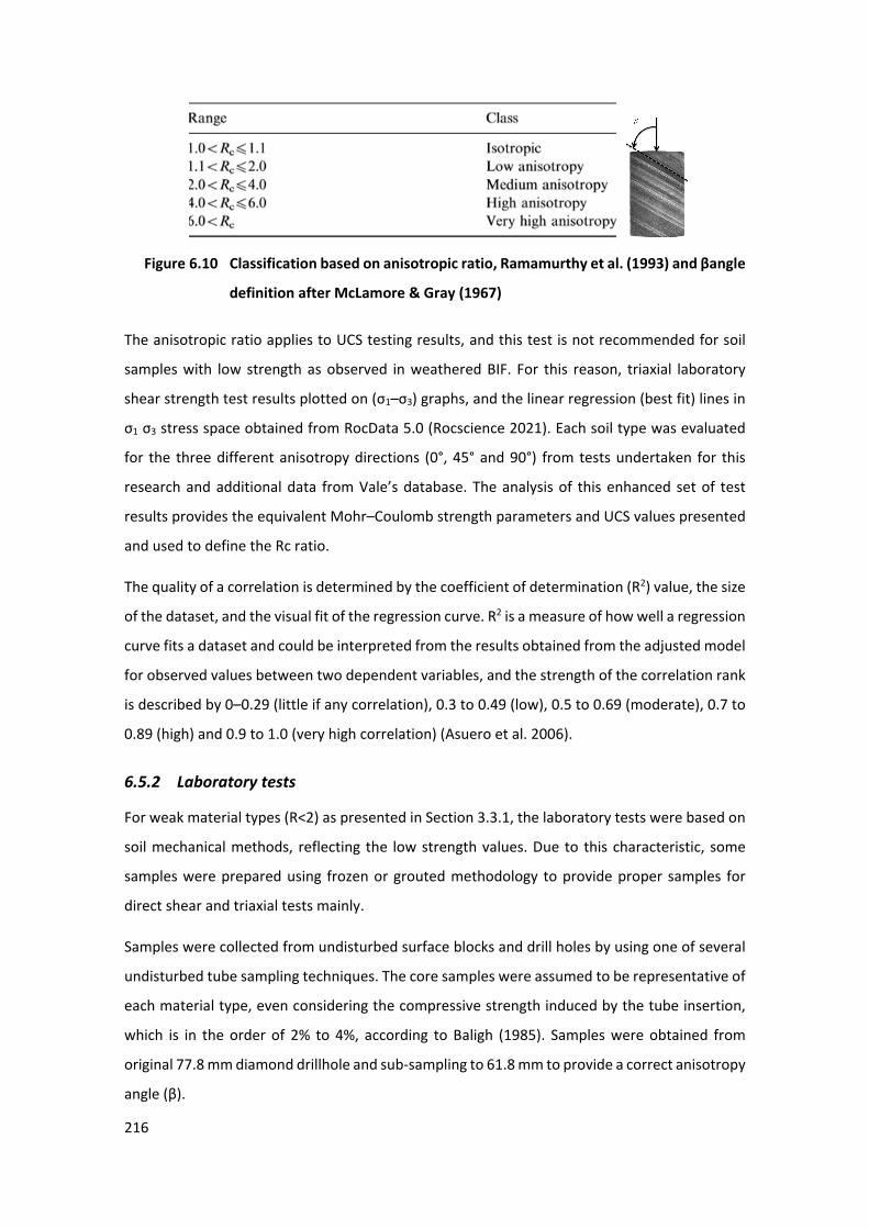
216
60 Figure 6.10 Classification based on anisotropic ratio, Ramamurthy et al. (1993) and βangle
definition after McLamore & Gray (1967)
The anisotropic ratio applies to UCS testing results, and this test is not recommended for soil
samples with low strength as observed in weathered BIF. For this reason, triaxial laboratory
shear strength test results plotted on (σ1–σ3) graphs, and the linear regression (best fit) lines in
σ1 σ3 stress space obtained from RocData 5.0 (Rocscience 2021). Each soil type was evaluated
for the three different anisotropy directions (0°, 45° and 90°) from tests undertaken for this
research and additional data from Vale’s database. The analysis of this enhanced set of test
results provides the equivalent Mohr–Coulomb strength parameters and UCS values presented
and used to define the Rc ratio.
The quality of a correlation is determined by the coefficient of determination (R2) value, the size
of the dataset, and the visual fit of the regression curve. R2 is a measure of how well a regression
curve fits a dataset and could be interpreted from the results obtained from the adjusted model
for observed values between two dependent variables, and the strength of the correlation rank
is described by 0–0.29 (little if any correlation), 0.3 to 0.49 (low), 0.5 to 0.69 (moderate), 0.7 to
0.89 (high) and 0.9 to 1.0 (very high correlation) (Asuero et al. 2006).
6.5.2 Laboratory tests
For weak material types (R<2) as presented in Section 3.3.1, the laboratory tests were based on
soil mechanical methods, reflecting the low strength values. Due to this characteristic, some
samples were prepared using frozen or grouted methodology to provide proper samples for
direct shear and triaxial tests mainly.
Samples were collected from undisturbed surface blocks and drill holes by using one of several
undisturbed tube sampling techniques. The core samples were assumed to be representative of
each material type, even considering the compressive strength induced by the tube insertion,
which is in the order of 2% to 4%, according to Baligh (1985). Samples were obtained from
original 77.8 mm diamond drillhole and sub-sampling to 61.8 mm to provide a correct anisotropy
angle (β).
217
Tests were undertaken in Brazil and Australia using standard tests according to the location of
the laboratory. Where necessary, the results were normalised to be properly compared. The
undertaken tests and standards are described in the following sections.
Petrographic thin sections description
Sample thin sections (perpendicular and parallel to banding) were prepared to evaluate crystal
and visual qualitative pore size, shape and percentage, mineralogy percentage and
micro-texture at the microscale for weathered BIF. A total of 15 thin sections were produced at
The University of Western Australia’s petrography laboratory and evaluated by Horta & Costa
(2016). Additionally, an extra 10 thin sections evaluated by Costa (2009), and another six thin
sections from a Vale internal report prepared by Zaparolli et al. (2007) were also used.
All samples were analysed using standard petrographic techniques based on a description table
created for better visualisation of the obtained information. This table contains a classification
of the soil type in the thin section, and important additional information observed during the
inspection. Microphotography was taken to show important features, textures, and
particularities.
The techniques used to determine size in thin sections are highly influenced by the angle at
which the banding is cut. For this reason, some bias is expected for these results. In order to
avoid this problem, only samples cut at 90° to the compositional metamorphic banding were
conducted for percentage proposals.
In situ and laboratory bulk density test
For the Brazilian laboratory, bulk density (𝜌𝜌b) of soil experiments in the laboratory was carried
out in accordance with ABNT NBR 16867 2020 (ABNT 2020), and for the Australian laboratory,
according to AS 1289.5.1.1-2017 (AS 2017). Additionally, results presented as Vale´s in situ 𝜌𝜌b
experiments were obtained by sand filled in accordance with NBR 7185/2016 (ABNT 2016) which
is applied to soils of any granulation that can be excavated with hand tools, and the pore spaces
need to be small enough not to be penetrated by the sand used during the experiment. Tested
material needs to be sufficiently cohesive and strong to avoid deformation during the
experiment.
Natural moisture content test
Natural moisture content of samples was based on removing moisture from samples by
oven-drying until its weight remains constant. Moisture content (%) was calculated from the
sample weight before and after drying. Experiments performed in Australia followed Standards
218
Association of Australia AS 1289.2.1.1 - 2005 (AS 2005) and NBR 6508/84 (ABNT 1984) for the
Brazilian laboratories.
In situ soil permeability test
In situ soil permeability tests were carried out to determine permeability coefficients of residual
soils and completely weathered rocks. Such experiments were carried out according to ABGE n°
04/1996 (ABGE 1996).
Particle size distribution and hydrometer
Particle size distribution (PSD) and hydrometer (sedimentation) tests were undertaken
according to AS 1289.3.6.1 -2009 (AS 2009), AS 1289.3.6.3.-2000 (AS 2000), and ASTM D422
2007 (ASTM 2007) at Australian laboratories and NBR 7217/1987 (ABNT 1987) at Brazilian
laboratories. For soil classification, USCS as defined in ASTM D-2487-98 (ASTM 1998) was used.
Atterberg limits
Atterberg limits (ATT) test were undertaken according to AS 1289.3.1.1 (AS 2009) and
AS 3.2.1 – 1995 (AS 2009) at Australian laboratories and NBR 7180 and NBR 6459 (ABNT 1984)
at Brazilian laboratories. The plasticity index was determined based on ASTM D4318-10 (ASTM
2010).
Constant and falling head (hydraulic conductivity) coefficient of permeability
The coefficients of permeability describe the rate at which a liquid moves through a soil
(hydraulic conductivity). Results are affected by fluid density and viscosity, void size, continuity,
soil particle shape, plasticity of the fines, and surface roughness. The coefficient of permeability
value is very often normalised to 20°C, marked as k20, since the viscosity of a fluid depends on
the temperature.
The constant head test was used for permeable soils (k>×10-6 m/s) and the falling head test for
less permeable soils (k<×10-9 m/s) to obtain the coefficient of permeability (k20). Tests were
undertaken according to AS 1289.6.2.1 (AS 2001) for constant head and AS 1289.6.7.2 (AS 2001)
for falling head in Australian laboratories and NBR 13292, (ABNT 1995) for constant head tests
and NBR 14545 (ABNT 2000) for variable head tests in Brazilian laboratories.
Bulk density
Bulk density was determined according to ASTM 1289.5.1.1:20017 (AS 2017) for Australian
laboratories and NBR 16867 (ABNT, 2001) for Brazilian laboratories. It was calculated according
to Equation 6.17.
219
ρb=𝑀𝑀𝑉𝑉
, (6.17)
where:
ρb = bulk density (kg/m3).
M = mass of the specimen measured prior to testing (kg).
V = volume (m3) of specimen calculated from dimensions measured during sample
preparation.
Natural moisture content
Natural moisture content testing was undertaken according to AS 1289.2.1.1 - 2005 (AS 2005)
in Australian laboratories and NBR 6508/84 (ABNT 1984) in Brazilian laboratories.
Single stage consolidated undrained triaxial compression test
For rock-like soils types, single stage, isotropic consolidated undrained tests (CIU) were
undertaken to determine the undrained strength (undrained condition) for a known initial
effective stress and a sample assumed fully saturated while monitoring the pore pressure during
shear. This does not allow drainage at all phases of the test, and is the most common test used
for weak, porous, and granular (permeable) materials. In view of the assumed high porosity of
the large majority of highly weathered BIF (except for the WAI and some WGI), this test was
considered to be the most appropriate method for establishing results in terms of total and
effective stress (with porewater pressure measurement). Results are presented as total or
effective stress and associated porewater pressure are determined for saturated behaviour.
Australian and Brazilian laboratory triaxial tests were undertaken according to ASTM D4767-95
(ASTM 1995) and both used cylindrical specimens with a diameter of 50 mm. Confinement
stresses (σ3) of 100 kPa, 200 kPa, 400 kPa, 600 kPa and 800 kPa were applied. Test stress levels
were limited to 800 kPa maximum due to a historical soil profile depth of 250 m for shallow
mines.
Single stage intact direct shear test under consolidated drained conditions
Brazilian and Australian laboratories undertook the drained single stage intact direct shear test
(IDST) under consolidated drained conditions tests following ASTM D-3080 (ASTM 2011) and
using normal stresses of 100 kPa, 200 kPa, 400 kPa, 600 kPa and 800 kPa. For better comparison
between the different materials, the total strain (displacement rate) was set to 8%.
220
Single stage intact unsaturated direct shear test with matric suction definition
The single stage intact unsaturated direct shear tests (UIDST) with matric suction definition were
undertaken only at an Australian laboratory. These were undertaken according to AS 1289.6.2.2
– 1998 (AS 1998) with some inhouse adequations using a modified apparatus as presented in
Figure 6.8A. The main modification is related to a high air entry disk installed in the pedestal of
the pressure cell that maintains the separation of the air and water pressures that are either
applied to or measured in the soil specimen. For this test, the sample is contained in a
conventional shear box which creates a predefined horizontal failure plane between the upper
and lower components of the shear box. The shear box was 60 mm long × 60 mm wide × 56 mm
deep.
The sample is sheared at a predefined βangle by trimming and inserting the sample in the shear
box with the anisotropic fabric at the required angle to the predefined horizontal failure plane
formed by the shear box.
The consolidated drained direct shear test on an unsaturated soil specimen can be conducted
using the modified direct shear apparatus shown in the cross-sectional view in Figure 6.8A. This
machine can perform unsaturated direct shear testing and pressure plate testing to obtain the
SWCC required for air entry value analysis and suction matric analysis determined by ASTM D
6836 02 (ASTM 2002)
The test procedure is similar to that used for a conventional direct shear apparatus. However,
as the laboratory responsible for carrying out this test uses an in-house adequation, the full text
procedures were presented here in accordance with Rahardjo & Fredlund (1996). From these
authors, the direct shear test apparatus consists of a split box with a top and bottom portion.
The soil specimen is sheared by moving the lower portion of the shear box relative to the upper
portion of the box. The shear box is housed in a pressure chamber.
A motor that provides a constant horizontal shear displacement rate is connected to the shear
box base. The shear box is seated on a pair of rollers that can move along grooved tracks on the
chamber base. The top box is connected to a load cell, which measures the shear load resistance.
Vacuum grease is placed between the two halves of the shear box prior to mounting the soil
specimen in the shear box. The plumbing layout for the control board of the modified direct
shear apparatus is similar to that used for a triaxial test; however, it is difficult to measure the
volume changes of the water because of the small water volumes involved. For this reason, the
saturation of the high air entry disk and the flushing of entrapped air from the base plate and its
connecting lines should be performed prior to commencing the test. The initial air and water
221
pressures to be applied to the soil specimen can be set on the pressure regulators while the soil
specimen is being assembled.
The tests are generally performed as consolidated drained direct shear tests. The soil specimen
is usually given access to water after being placed into the direct shear box. The soil sample
needs to be fully saturated prior to being placed into the cell to ensure the test is started off on
the drying curve from the SWCC so the correct matric suctions are applied to obtain the correct
moisture content. For dry and wet curve validation tests the moisture content must be a
minimum of 0.5%, and for matric suction of 1 MPa or 1.5 MPa a maximum of 40% used to define
SWCC curves.
The chamber cap is applied following saturation of the soil. The predetermined vertical normal
load, air pressure, and water pressure are then applied to the specimen in this sequence. The
vertical normal load is applied through the loading ram at the same time that the air and water
pressures are applied.
Once the sample is placed into the cell, a check of the Skempton’s parameter ‘B’ response is
required. This should be 0.98 and above. The sample is then allowed to consolidate vertically
using an applied normal stress.
A secondary consolidation phase is required using the matric suction once the vertical
consolidation is complete. Shearing should be slow enough to ensure the equalisation of the
vapour loss and pore pressure so that matric suction remains constant.
The soil specimen is sheared at an approximate horizontal shear displacement rate after
equilibration has been reached. The horizontal shear load resistance is measured using a load
cell. Readings are also taken of vertical deformation, horizontal shear displacement, and water
volume change during shear. Shearing can be terminated either when the horizontal shear stress
resistance has reached its peak value or when the horizontal shear displacement has reached a
designated limiting value. In the case of a multistage test, the shearing process for each stage
should be stopped when the peak horizontal shear stress appears to be imminent.
Direct shear testing equipment was set with a constant horizontal displacement rate of
0.2 mm/minute, which was sufficient to ensure the tests were in a drained condition for the
coarse tested materials (WHE and WQI). A datalogger was used to record vertical displacement,
horizontal displacement, and shear force at 10 second intervals. Maximum horizontal
displacement was set to 7 mm. Soil specimens were sheared using a vertical stress between
222
75 kPa to 100 kPa. Peak shear stress for the unsaturated sample was recorded at different
predefined matric suction.
As already mentioned, the Vale database and previous laboratory reports have provided
additional laboratory test results used in this research. Only data that could be associated with
anisotropy, bulk density values and geomechanical classification equal to the ones used in the
present study were considered, each associated to a specific material type.
Summing up, the laboratory campaign consisted of tests carried out exclusively for this research,
results extracted from Costa (2009) and Zapparoli et al. (2007) and those from the Vale database
as shown in Table 6.1. Used test results are available at Appendices VI, VII, and VIII.
16 Table 6.1 Testing summary table
Laboratory tests n (Vale database) n (tested) n (total)
Thin sections 16 15 25
PSD – 23 23
ATT – 17 17
K20 – 26 26
UIDST – 52 52
IDST 23 60 83
CU 24 91 115
SWCC – 18 18
6.6 RESULTS
6.6.1 Fabric and mineralogical thin section overview
From the microscope studies of completely to highly weathered material it was possible to verify
mineralogy, visual total porosity, and textural features characteristics as described in the
following sections. Some of these micro-features are responsible for the geomechanical
behaviour observed in these weak material types.
• Weak hematitite
The weak hematitite (WHE) is basically composed of hematite and martite growing over
a granoblastic fabric (0.02 mm to 1.4 mm), as seen in Figure 6.11A and presents strong
heterogeneity when it occurs associated with lamellar iron minerals in the shape of
specularite (0.07 mm long and 0.01 mm wide), or moderate heterogeneity when
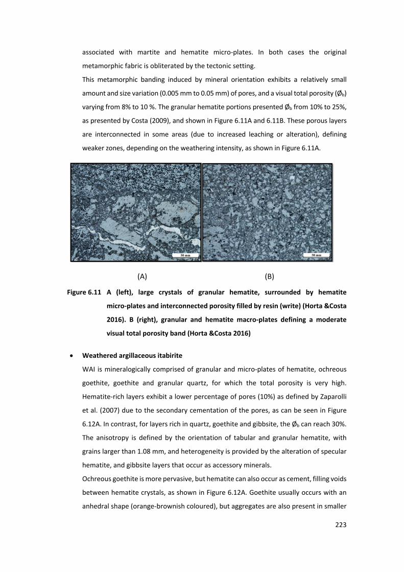
223
associated with martite and hematite micro-plates. In both cases the original
metamorphic fabric is obliterated by the tectonic setting.
This metamorphic banding induced by mineral orientation exhibits a relatively small
amount and size variation (0.005 mm to 0.05 mm) of pores, and a visual total porosity (Øb)
varying from 8% to 10 %. The granular hematite portions presented Øb from 10% to 25%,
as presented by Costa (2009), and shown in Figure 6.11A and 6.11B. These porous layers
are interconnected in some areas (due to increased leaching or alteration), defining
weaker zones, depending on the weathering intensity, as shown in Figure 6.11A.
(A) (B)
61 Figure 6.11 A (left), large crystals of granular hematite, surrounded by hematite
micro-plates and interconnected porosity filled by resin (write) (Horta &Costa
2016). B (right), granular and hematite macro-plates defining a moderate
visual total porosity band (Horta &Costa 2016)
• Weathered argillaceous itabirite
WAI is mineralogically comprised of granular and micro-plates of hematite, ochreous
goethite, goethite and granular quartz, for which the total porosity is very high.
Hematite-rich layers exhibit a lower percentage of pores (10%) as defined by Zaparolli
et al. (2007) due to the secondary cementation of the pores, as can be seen in Figure
6.12A. In contrast, for layers rich in quartz, goethite and gibbsite, the Øb can reach 30%.
The anisotropy is defined by the orientation of tabular and granular hematite, with
grains larger than 1.08 mm, and heterogeneity is provided by the alteration of specular
hematite, and gibbsite layers that occur as accessory minerals.
Ochreous goethite is more pervasive, but hematite can also occur as cement, filling voids
between hematite crystals, as shown in Figure 6.12A. Goethite usually occurs with an
anhedral shape (orange-brownish coloured), but aggregates are also present in smaller
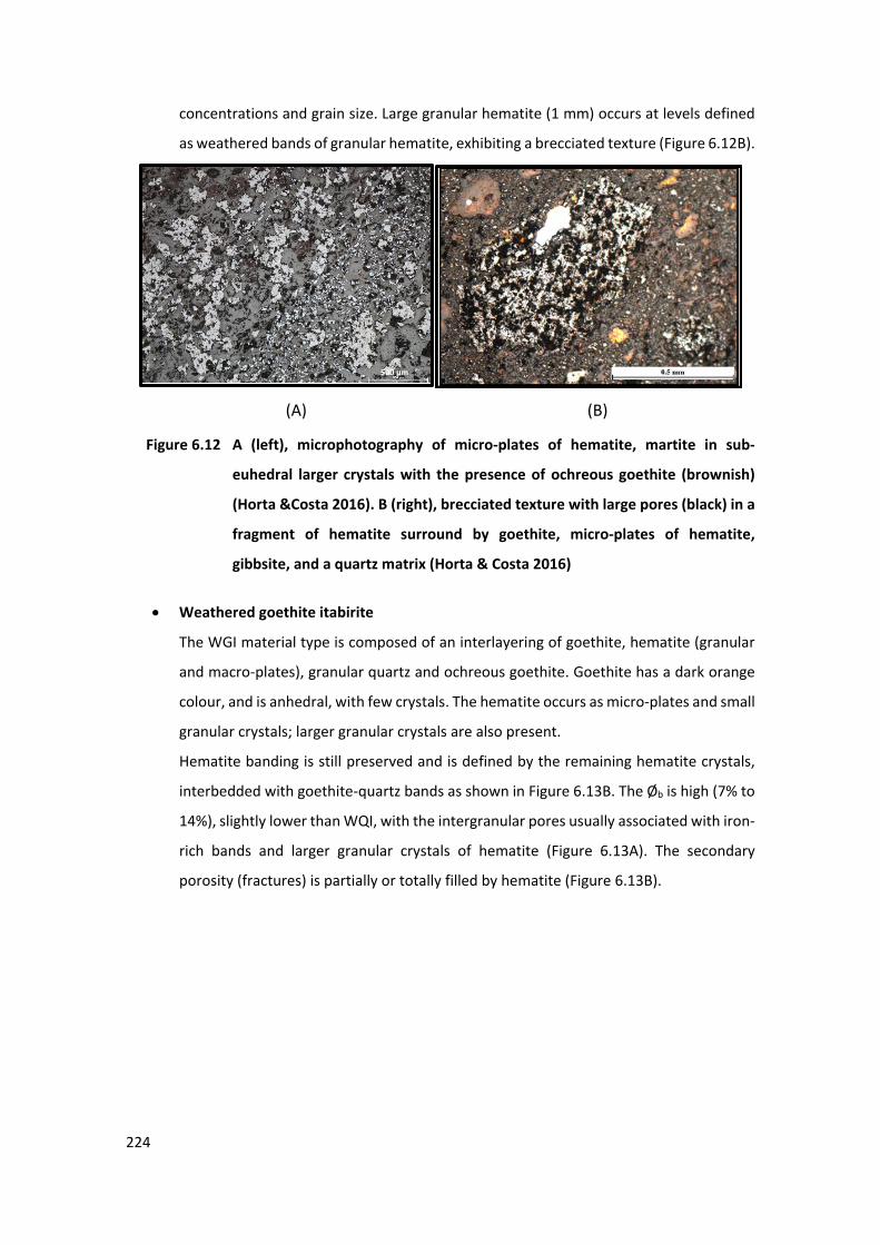
224
concentrations and grain size. Large granular hematite (1 mm) occurs at levels defined
as weathered bands of granular hematite, exhibiting a brecciated texture (Figure 6.12B).
(A) (B)
62 Figure 6.12 A (left), microphotography of micro-plates of hematite, martite in sub-
euhedral larger crystals with the presence of ochreous goethite (brownish)
(Horta &Costa 2016). B (right), brecciated texture with large pores (black) in a
fragment of hematite surround by goethite, micro-plates of hematite,
gibbsite, and a quartz matrix (Horta & Costa 2016)
• Weathered goethite itabirite
The WGI material type is composed of an interlayering of goethite, hematite (granular
and macro-plates), granular quartz and ochreous goethite. Goethite has a dark orange
colour, and is anhedral, with few crystals. The hematite occurs as micro-plates and small
granular crystals; larger granular crystals are also present.
Hematite banding is still preserved and is defined by the remaining hematite crystals,
interbedded with goethite-quartz bands as shown in Figure 6.13B. The Øb is high (7% to
14%), slightly lower than WQI, with the intergranular pores usually associated with iron-
rich bands and larger granular crystals of hematite (Figure 6.13A). The secondary
porosity (fractures) is partially or totally filled by hematite (Figure 6.13B).
500 μm
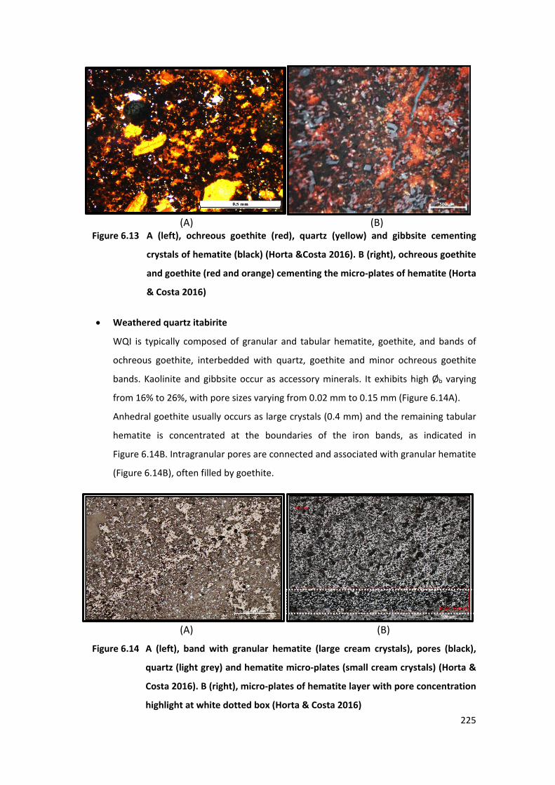
225
(A) (B) 63 Figure 6.13 A (left), ochreous goethite (red), quartz (yellow) and gibbsite cementing
crystals of hematite (black) (Horta &Costa 2016). B (right), ochreous goethite
and goethite (red and orange) cementing the micro-plates of hematite (Horta
& Costa 2016)
• Weathered quartz itabirite
WQI is typically composed of granular and tabular hematite, goethite, and bands of
ochreous goethite, interbedded with quartz, goethite and minor ochreous goethite
bands. Kaolinite and gibbsite occur as accessory minerals. It exhibits high Øb varying
from 16% to 26%, with pore sizes varying from 0.02 mm to 0.15 mm (Figure 6.14A).
Anhedral goethite usually occurs as large crystals (0.4 mm) and the remaining tabular
hematite is concentrated at the boundaries of the iron bands, as indicated in
Figure 6.14B. Intragranular pores are connected and associated with granular hematite
(Figure 6.14B), often filled by goethite.
(A) (B)
64 Figure 6.14 A (left), band with granular hematite (large cream crystals), pores (black),
quartz (light grey) and hematite micro-plates (small cream crystals) (Horta &
Costa 2016). B (right), micro-plates of hematite layer with pore concentration
highlight at white dotted box (Horta & Costa 2016)
1 mm
500 μm
500 μm 1,000 μm
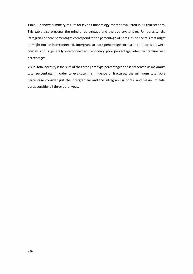
226
Table 6.2 shows summary results for Øb and mineralogy content evaluated in 31 thin sections.
This table also presents the mineral percentage and average crystal size. For porosity, the
intragranular pore percentages correspond to the percentage of pores inside crystals that might
or might not be interconnected. Intergranular pore percentage correspond to pores between
crystals and is generally interconnected. Secondary pore percentage refers to fracture void
percentages.
Visual total porosity is the sum of the three pore type percentages and is presented as maximum
total percentage. In order to evaluate the influence of fractures, the minimum total pore
percentage consider just the intergranular and the intragranular pores, and maximum total
pores consider all three pore types.
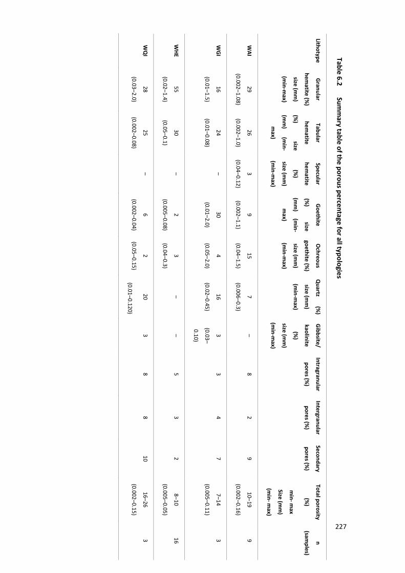
17 Table 6.2 Sum
mary table of the porous percentage for all typologies
Lithotype G
ranular
hematite (%
)
size (mm
)
(min-m
ax)
Tabular
hematite
(%) size
(mm
)(m
in-
max)
Specular
hematite
(%)
size (mm
)
(min-m
ax)
Goethite
(%) size
(mm
)(m
in-
max)
Ochreous
goethite (%)
size (mm
)
(min-m
ax)
Quartz (%
)
size (mm
)
(min-m
ax)
Gibbsite/
kaolinite
(%)
size (mm
)
(min-m
ax)
Intragranular
pores (%)
Intergranular
pores (%)
Secondary
pores (%)
Total porosity
(%)
min- m
ax
Size (mm
)
(min- m
ax)
n
(samples)
WAI
29
(0.002–1.08)
26
(0.002–1.0)
3
(0.04–0.12)
9
(0.002–1.1)
15
(0.04–1.5)
7
(0.006–0.3)
–8
2 9
10–19
(0.002–0.16)
9
WG
I 16
(0.01–1.5)
24
(0.01–0.08)
–30
(0.01–2.0)
4
(0.05–2.0)
16
(0.02–0.45)
3
(0.03–
0.10)
3 4
7 7–14
(0.005–0.11)
3
WH
E 55
(0.02–1.4)
30
(0.05–0.1)
–2
(0.005–0.08)
3
(0.04–0.3)
– –
5 3
2 8–10
(0.005–0.05)
16
WQ
I 28
(0.03–2.0)
25
(0.002–0.08)
–6
(0.002–0.04)
2
(0.05–0.15)
20
(0.01–0.120)
3 8
8 10
16–26
(0.002–0.15)
3
227
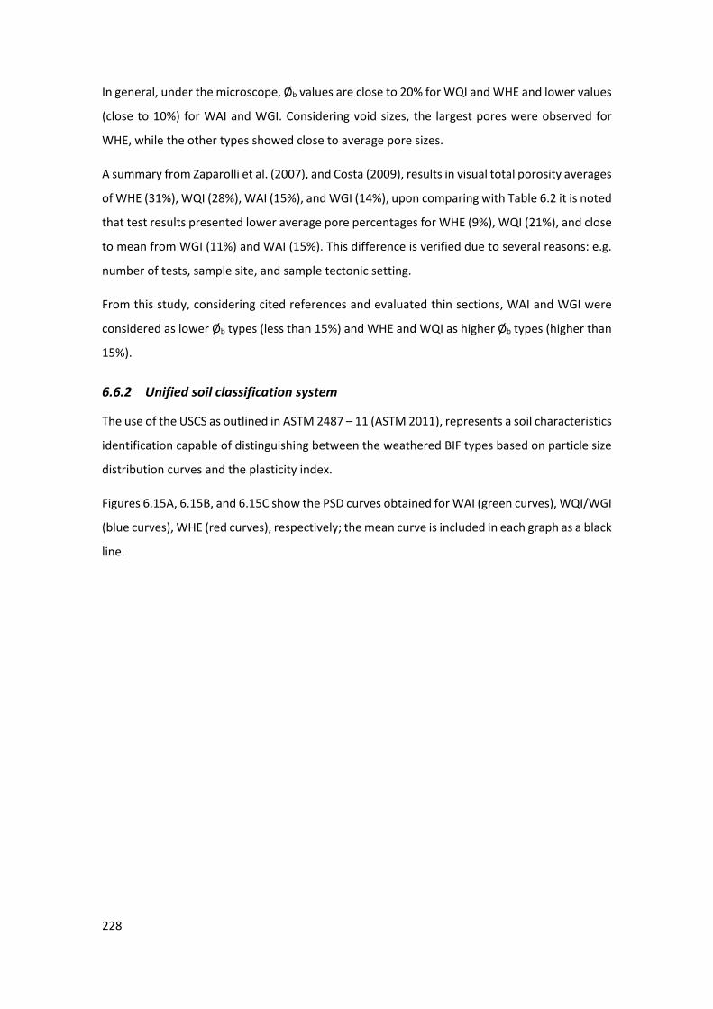
228
In general, under the microscope, Øb values are close to 20% for WQI and WHE and lower values
(close to 10%) for WAI and WGI. Considering void sizes, the largest pores were observed for
WHE, while the other types showed close to average pore sizes.
A summary from Zaparolli et al. (2007), and Costa (2009), results in visual total porosity averages
of WHE (31%), WQI (28%), WAI (15%), and WGI (14%), upon comparing with Table 6.2 it is noted
that test results presented lower average pore percentages for WHE (9%), WQI (21%), and close
to mean from WGI (11%) and WAI (15%). This difference is verified due to several reasons: e.g.
number of tests, sample site, and sample tectonic setting.
From this study, considering cited references and evaluated thin sections, WAI and WGI were
considered as lower Øb types (less than 15%) and WHE and WQI as higher Øb types (higher than
15%).
6.6.2 Unified soil classification system
The use of the USCS as outlined in ASTM 2487 – 11 (ASTM 2011), represents a soil characteristics
identification capable of distinguishing between the weathered BIF types based on particle size
distribution curves and the plasticity index.
Figures 6.15A, 6.15B, and 6.15C show the PSD curves obtained for WAI (green curves), WQI/WGI
(blue curves), WHE (red curves), respectively; the mean curve is included in each graph as a black
line.
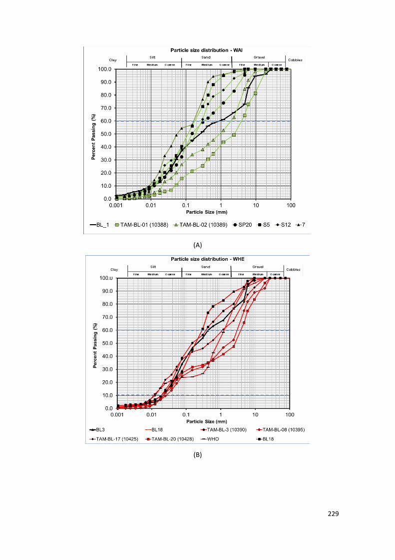
229
(A)
(B)
230
(C)
65 Figure 6.15 A (top), WAI PSD curves – green. B (centre), WHE PSD curves – red. C (bottom),
WQI and WGI PSD curves – cyan. Black curves are the mean value for each type
A certain amount of dispersion for each group is noted; this could be attributed to heterogeneity
caused by different layer thicknesses of iron or non-iron bands that could result in physical and
chemical dispersion for the same material type. Due to the small number of WGI test results and
similarities with WQI results, these two types were grouped for the next evaluations. Table 6.3
presents the percentage content for each particle size distribution (PSD) and textural USCS soil
classification in accordance with ASTM D2487-11 (ASTM 2011).
Table 6.3 also presents the Atterberg limits results for fractions below 425 μm for each material
type and the ρb values. Empirical Atterberg limits describe how moisture content and intrinsic
soil characteristics interact to convey their elasto-plastic behaviour. These tests allow
classification and identification of the fine soil fraction and complete the USCS classification.
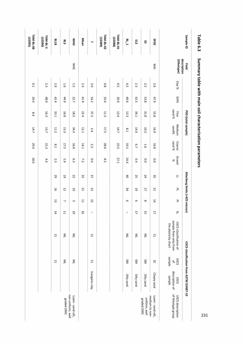
18 Table 6.3 Sum
mary table w
ith main soil characterisation param
eters
Sample ID
Field
description (lithotype)
PSD (total sample)
Atterberg limits (<425 m
icron) U
SCS classification from ASTM
D2487-10
Clay %
Silt%
Fine sand %
M
edium
sand%
Coarse sand %
Gravel
%
LL PL
PI SL
USCS classification of
sample fines only from
the plasticity chart
USCS of
sample
USCS
description of sam
ple
USCS description
of lithotype group
SP20 W
AI 2.6
47.9 15.8
16.9 16.8
0.0 35
21 14
17 CL
SC Clayey sand
Loam - sand-silt,
medium
to non-uniform
, well
graded (SM)
S5 2.5
53.8 31.8
10.3 1.6
0.0 24
17 8
15 M
L SM
Silty sand
S12 2.3
42.5 34.1
14.0 6.7
0.4 25
19 6
17 M
L SM
Silty sand
BL_1 4.5
40.6 13.3
8.1 19.1
14.4 40
34 6
– M
LSM
Silty sand
TAM-BL-01
(10388) 0.5
20.9 13.4
14.7 23.5
27.1
TAM-BL-02
(10389) 0.8
33.4 11.3
17.5 28.6
8.5
7 3.0
54.2 37.2
3.4 2.2
0.0 37
15 22
– CL
CL Inorganic clay
Mean
2.3 41.9
22.4 12.1
14.1 7.2
32 21
11 16
WHO
W
HE 1.5
22.7 18.5
34.4 16.6
6.3 22
19 3
19 M
L M
L Loam
- sand-silt, non-uniform
, well
graded (SM)
BL3 1.6
44.9 16.8
13.3 17.5
5.9 19
12 7
11 M
L M
L
BL18 2.9
42.4 33.1
11.2 8.1
2.3 29
16 13
14 CL
CL
TAM-BL-3
(10390) 2.3
48.0 16.3
13.7 15.3
4.4
TAM-BL-08
(10395) 0.1
29.4 8.4
14.7 29.4
18.0
231
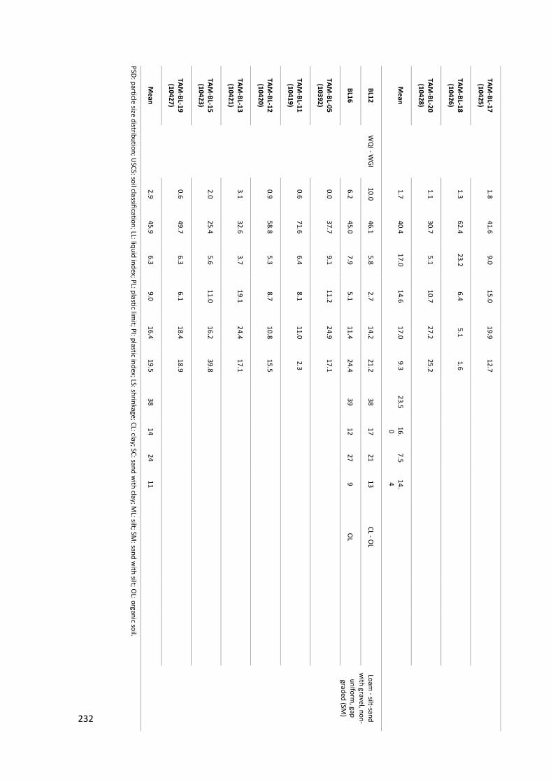
TAM-BL-17
(10425) 1.8
41.6 9.0
15.0 19.9
12.7
TAM-BL-18
(10426) 1.3
62.4 23.2
6.4 5.1
1.6
TAM-BL-20
(10428) 1.1
30.7 5.1
10.7 27.2
25.2
Mean
1.7 40.4
17.0 14.6
17.0 9.3
23.5 16.0
7.5 14.4
BL12 W
QI - W
GI 10.0
46.1 5.8
2.7 14.2
21.2 38
17 21
13 CL - O
L Loam
- silt-sand w
ith gravel, non-uniform
, gap graded (SM
) BL16
6.2 45.0
7.9 5.1
11.4 24.4
39 12
27 9
OL
TAM-BL-05
(10392) 0.0
37.7 9.1
11.2 24.9
17.1
TAM-BL-11
(10419) 0.6
71.6 6.4
8.1 11.0
2.3
TAM-BL-12
(10420) 0.9
58.8 5.3
8.7 10.8
15.5
TAM-BL-13
(10421) 3.1
32.6 3.7
19.1 24.4
17.1
TAM-BL-15
(10423) 2.0
25.4 5.6
11.0 16.2
39.8
TAM-BL-19
(10427) 0.6
49.7 6.3
6.1 18.4
18.9
Mean
2.9 45.9
6.3 9.0
16.4 19.5
38 14
24 11
PSD: particle size distribution; USCS: soil classification; LL: liquid index; PL: plastic lim
it; PI: plastic index; LS: shrinkage; CL: clay; SC: sand with clay; M
L: silt; SM: sand w
ith silt; OL: organic soil.
232
233
Considering the PSD, results of the WAI and WHE have similarities: a lower percentage of gravel (less
than 10%) and higher fine and medium sand percentages (higher than 30%). WQI and WGI have a
higher relative gravel percentage (20%) and lower fine and medium sand percentages (15%).
Based on USCS classification and the shape of PSD curves, WAI and WHE (SM) exhibit a similar
classification to ’fine-grained soils’ or ‘silt-sand soils‘, with curves well graded and non-uniform.
WQI/WGI (MS) were classified as gravel soil gap graded, mixed grained soil or silt-sand soils,
with a gap in the size of fine to medium sand. In general, all curves were shown to be
non-uniform and with a higher individual percentage of silt (a variation between silt and sand
fraction content is observed for each material).
WAI displays a high dispersion in the plasticity chart; however, it is mainly silt (ML) with a low
plasticity except for one sample showing high plasticity (sample WAI 3). The sample WAI 3 result
came from a single layer of high clay content and low activity (gibbsite and kaolinite). WHE and
WQI/WGI exhibit a dual classification with a group plotted in silt (ML) with low plasticity and
another group with intermediate plasticity (CL).
The clay size fraction percentage varies from 2% to 3% in average and can reach 10% in some
samples (WAI 3). This clay content is in part related to kaolinite and gibbsite (low activity
minerals) and another part (percentage not evaluated) is composed of clay size minerals
composed basically of non-clay minerals such as iron oxides and hydroxides, including goethite
and ochreous goethite.
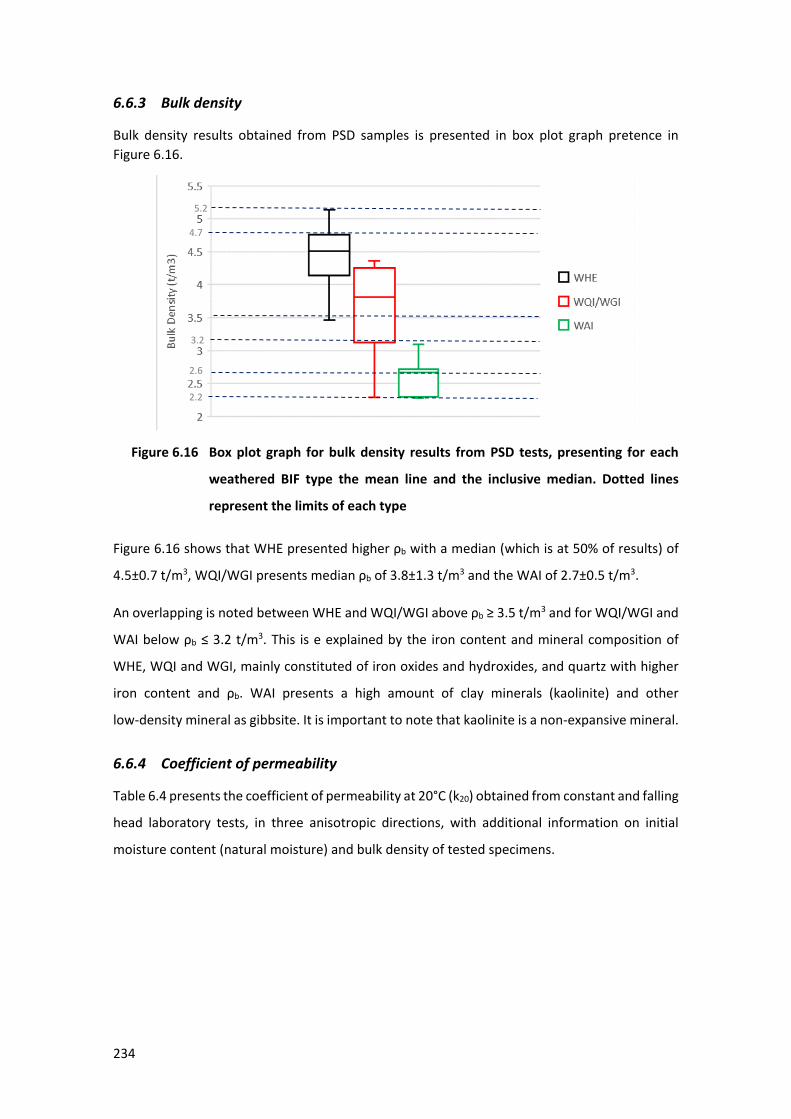
234
6.6.3 Bulk density
Bulk density results obtained from PSD samples is presented in box plot graph pretence in Figure 6.16.
66 Figure 6.16 Box plot graph for bulk density results from PSD tests, presenting for each
weathered BIF type the mean line and the inclusive median. Dotted lines
represent the limits of each type
Figure 6.16 shows that WHE presented higher ρb with a median (which is at 50% of results) of
4.5±0.7 t/m3, WQI/WGI presents median ρb of 3.8±1.3 t/m3 and the WAI of 2.7±0.5 t/m3.
An overlapping is noted between WHE and WQI/WGI above ρb ≥ 3.5 t/m3 and for WQI/WGI and
WAI below ρb ≤ 3.2 t/m3. This is e explained by the iron content and mineral composition of
WHE, WQI and WGI, mainly constituted of iron oxides and hydroxides, and quartz with higher
iron content and ρb. WAI presents a high amount of clay minerals (kaolinite) and other
low-density mineral as gibbsite. It is important to note that kaolinite is a non-expansive mineral.
6.6.4 Coefficient of permeability
Table 6.4 presents the coefficient of permeability at 20°C (k20) obtained from constant and falling
head laboratory tests, in three anisotropic directions, with additional information on initial
moisture content (natural moisture) and bulk density of tested specimens.
3.2
2.2
4.7
2.6
5.2
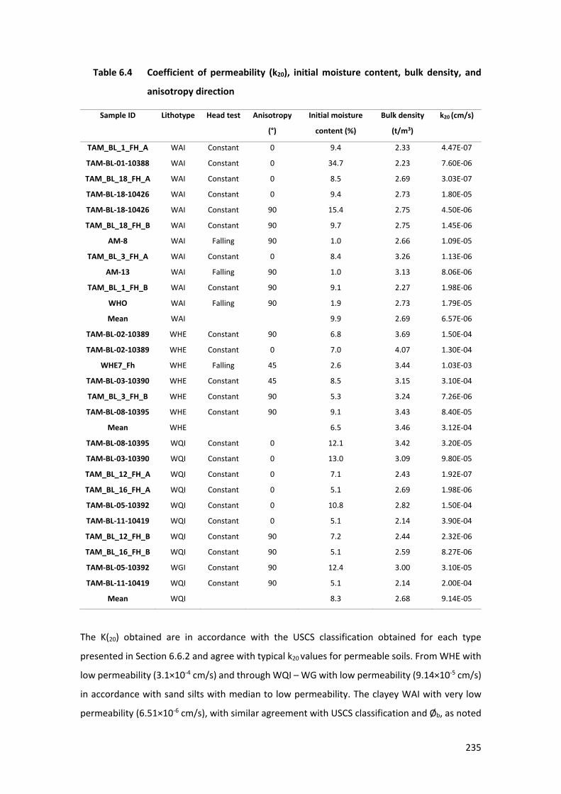
235
19 Table 6.4 Coefficient of permeability (k20), initial moisture content, bulk density, and
anisotropy direction
Sample ID Lithotype Head test Anisotropy
(°)
Initial moisture
content (%)
Bulk density
(t/m3)
k20 (cm/s)
TAM_BL_1_FH_A WAI Constant 0 9.4 2.33 4.47E-07
TAM-BL-01-10388 WAI Constant 0 34.7 2.23 7.60E-06
TAM_BL_18_FH_A WAI Constant 0 8.5 2.69 3.03E-07
TAM-BL-18-10426 WAI Constant 0 9.4 2.73 1.80E-05
TAM-BL-18-10426 WAI Constant 90 15.4 2.75 4.50E-06
TAM_BL_18_FH_B WAI Constant 90 9.7 2.75 1.45E-06
AM-8 WAI Falling 90 1.0 2.66 1.09E-05
TAM_BL_3_FH_A WAI Constant 0 8.4 3.26 1.13E-06
AM-13 WAI Falling 90 1.0 3.13 8.06E-06
TAM_BL_1_FH_B WAI Constant 90 9.1 2.27 1.98E-06
WHO WAI Falling 90 1.9 2.73 1.79E-05
Mean WAI
9.9 2.69 6.57E-06
TAM-BL-02-10389 WHE Constant 90 6.8 3.69 1.50E-04
TAM-BL-02-10389 WHE Constant 0 7.0 4.07 1.30E-04
WHE7_Fh WHE Falling 45 2.6 3.44 1.03E-03
TAM-BL-03-10390 WHE Constant 45 8.5 3.15 3.10E-04
TAM_BL_3_FH_B WHE Constant 90 5.3 3.24 7.26E-06
TAM-BL-08-10395 WHE Constant 90 9.1 3.43 8.40E-05
Mean WHE
6.5 3.46 3.12E-04
TAM-BL-08-10395 WQI Constant 0 12.1 3.42 3.20E-05
TAM-BL-03-10390 WQI Constant 0 13.0 3.09 9.80E-05
TAM_BL_12_FH_A WQI Constant 0 7.1 2.43 1.92E-07
TAM_BL_16_FH_A WQI Constant 0 5.1 2.69 1.98E-06
TAM-BL-05-10392 WQI Constant 0 10.8 2.82 1.50E-04
TAM-BL-11-10419 WQI Constant 0 5.1 2.14 3.90E-04
TAM_BL_12_FH_B WQI Constant 90 7.2 2.44 2.32E-06
TAM_BL_16_FH_B WQI Constant 90 5.1 2.59 8.27E-06
TAM-BL-05-10392 WGI Constant 90 12.4 3.00 3.10E-05
TAM-BL-11-10419 WQI Constant 90 5.1 2.14 2.00E-04
Mean WQI
8.3 2.68 9.14E-05
The K(20) obtained are in accordance with the USCS classification obtained for each type
presented in Section 6.6.2 and agree with typical k20 values for permeable soils. From WHE with
low permeability (3.1×10⁻⁴ cm/s) and through WQI – WG with low permeability (9.14×10⁻⁵ cm/s)
in accordance with sand silts with median to low permeability. The clayey WAI with very low
permeability (6.51×10⁻⁶ cm/s), with similar agreement with USCS classification and Øb, as noted
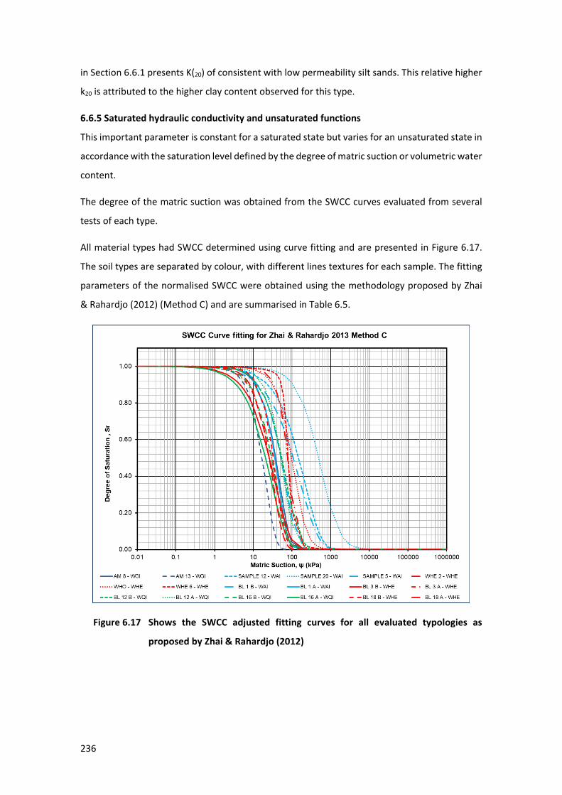
236
in Section 6.6.1 presents K(20) of consistent with low permeability silt sands. This relative higher
k20 is attributed to the higher clay content observed for this type.
6.6.5 Saturated hydraulic conductivity and unsaturated functions
This important parameter is constant for a saturated state but varies for an unsaturated state in
accordance with the saturation level defined by the degree of matric suction or volumetric water
content.
The degree of the matric suction was obtained from the SWCC curves evaluated from several
tests of each type.
All material types had SWCC determined using curve fitting and are presented in Figure 6.17.
The soil types are separated by colour, with different lines textures for each sample. The fitting
parameters of the normalised SWCC were obtained using the methodology proposed by Zhai
& Rahardjo (2012) (Method C) and are summarised in Table 6.5.
67 Figure 6.17 Shows the SWCC adjusted fitting curves for all evaluated typologies as
proposed by Zhai & Rahardjo (2012)
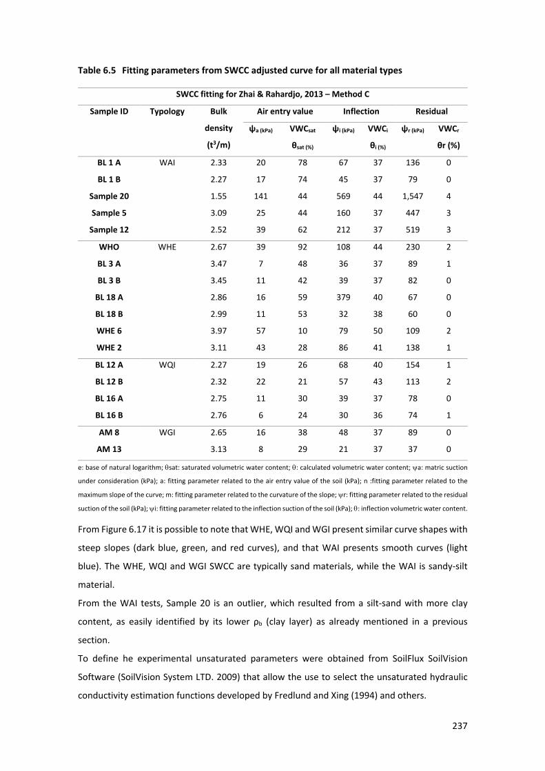
237
Table 6.5 Fitting parameters from SWCC adjusted curve for all material types
SWCC fitting for Zhai & Rahardjo, 2013 – Method C
Sample ID Typology Bulk
density
(t3/m)
Air entry value Inflection Residual
ψa (kPa) VWCsat
θsat (%)
ψi (kPa) VWCi
θi (%)
ψr (kPa) VWCr
θr (%)
BL 1 A WAI 2.33 20 78 67 37 136 0
BL 1 B 2.27 17 74 45 37 79 0
Sample 20 1.55 141 44 569 44 1,547 4
Sample 5 3.09 25 44 160 37 447 3
Sample 12 2.52 39 62 212 37 519 3
WHO WHE 2.67 39 92 108 44 230 2
BL 3 A 3.47 7 48 36 37 89 1
BL 3 B 3.45 11 42 39 37 82 0
BL 18 A 2.86 16 59 379 40 67 0
BL 18 B 2.99 11 53 32 38 60 0
WHE 6 3.97 57 10 79 50 109 2
WHE 2 3.11 43 28 86 41 138 1
BL 12 A WQI 2.27 19 26 68 40 154 1
BL 12 B 2.32 22 21 57 43 113 2
BL 16 A 2.75 11 30 39 37 78 0
BL 16 B 2.76 6 24 30 36 74 1
AM 8 WGI 2.65 16 38 48 37 89 0
AM 13 3.13 8 29 21 37 37 0
e: base of natural logarithm; θsat: saturated volumetric water content; θ: calculated volumetric water content; ψa: matric suction
under consideration (kPa); a: fitting parameter related to the air entry value of the soil (kPa); n :fitting parameter related to the
maximum slope of the curve; m: fitting parameter related to the curvature of the slope; ψr: fitting parameter related to the residual
suction of the soil (kPa); ψi: fitting parameter related to the inflection suction of the soil (kPa); θ: inflection volumetric water content.
From Figure 6.17 it is possible to note that WHE, WQI and WGI present similar curve shapes with
steep slopes (dark blue, green, and red curves), and that WAI presents smooth curves (light
blue). The WHE, WQI and WGI SWCC are typically sand materials, while the WAI is sandy-silt
material.
From the WAI tests, Sample 20 is an outlier, which resulted from a silt-sand with more clay
content, as easily identified by its lower ρb (clay layer) as already mentioned in a previous
section.
To define he experimental unsaturated parameters were obtained from SoilFlux SoilVision
Software (SoilVision System LTD. 2009) that allow the use to select the unsaturated hydraulic
conductivity estimation functions developed by Fredlund and Xing (1994) and others.
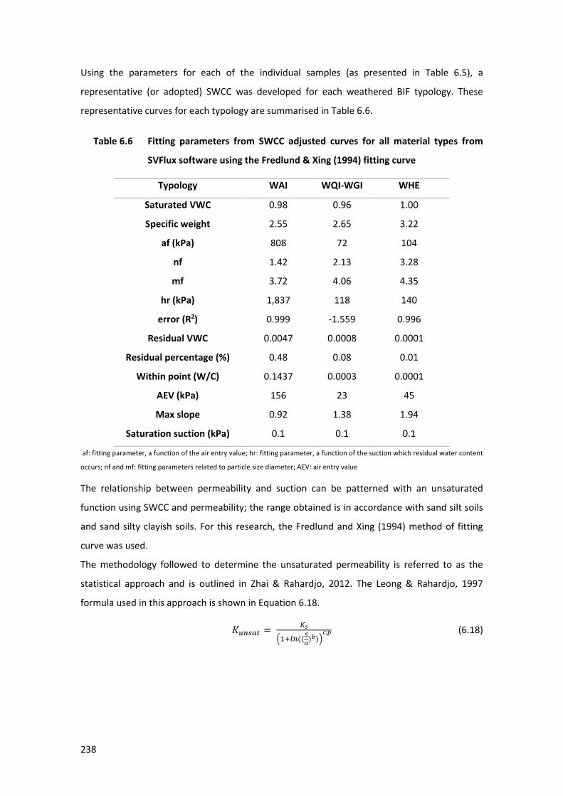
238
Using the parameters for each of the individual samples (as presented in Table 6.5), a
representative (or adopted) SWCC was developed for each weathered BIF typology. These
representative curves for each typology are summarised in Table 6.6.
20 Table 6.6 Fitting parameters from SWCC adjusted curves for all material types from
SVFlux software using the Fredlund & Xing (1994) fitting curve
Typology WAI WQI-WGI WHE
Saturated VWC 0.98 0.96 1.00
Specific weight 2.55 2.65 3.22
af (kPa) 808 72 104
nf 1.42 2.13 3.28
mf 3.72 4.06 4.35
hr (kPa) 1,837 118 140
error (R2) 0.999 -1.559 0.996
Residual VWC 0.0047 0.0008 0.0001
Residual percentage (%) 0.48 0.08 0.01
Within point (W/C) 0.1437 0.0003 0.0001
AEV (kPa) 156 23 45
Max slope 0.92 1.38 1.94
Saturation suction (kPa) 0.1 0.1 0.1
af: fitting parameter, a function of the air entry value; hr: fitting parameter, a function of the suction which residual water content
occurs; nf and mf: fitting parameters related to particle size diameter; AEV: air entry value
The relationship between permeability and suction can be patterned with an unsaturated
function using SWCC and permeability; the range obtained is in accordance with sand silt soils
and sand silty clayish soils. For this research, the Fredlund and Xing (1994) method of fitting
curve was used.
The methodology followed to determine the unsaturated permeability is referred to as the
statistical approach and is outlined in Zhai & Rahardjo, 2012. The Leong & Rahardjo, 1997
formula used in this approach is shown in Equation 6.18.
𝐾𝐾𝑢𝑢𝑚𝑚𝑢𝑢𝑎𝑎𝑢𝑢 = 𝐾𝐾𝑠𝑠
�1+𝑙𝑙𝑚𝑚((𝑆𝑆𝑎𝑎)𝑏𝑏)�𝑐𝑐.𝑝𝑝 (6.18)
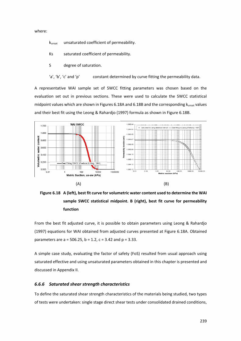
239
where:
kunsat unsaturated coefficient of permeability.
Ks saturated coefficient of permeability.
S degree of saturation.
‘a’, ‘b’, ‘c’ and ‘p’ constant determined by curve fitting the permeability data.
A representative WAI sample set of SWCC fitting parameters was chosen based on the
evaluation set out in previous sections. These were used to calculate the SWCC statistical
midpoint values which are shown in Figures 6.18A and 6.18B and the corresponding kunsat values
and their best fit using the Leong & Rahardjo (1997) formula as shown in Figure 6.18B.
(A) (B)
68 Figure 6.18 A (left), best fit curve for volumetric water content used to determine the WAI
sample SWCC statistical midpoint. B (right), best fit curve for permeability
function
From the best fit adjusted curve, it is possible to obtain parameters using Leong & Rahardjo
(1997) equations for WAI obtained from adjusted curves presented at Figure 6.18A. Obtained
parameters are a = 506.25, b = 1.2, c = 3.42 and p = 3.33.
A simple case study, evaluating the factor of safety (FoS) resulted from usual approach using
saturated effective and using unsaturated parameters obtained in this chapter is presented and
discussed in Appendix II.
6.6.6 Saturated shear strength characteristics
To define the saturated shear strength characteristics of the materials being studied, two types
of tests were undertaken: single stage direct shear tests under consolidated drained conditions,
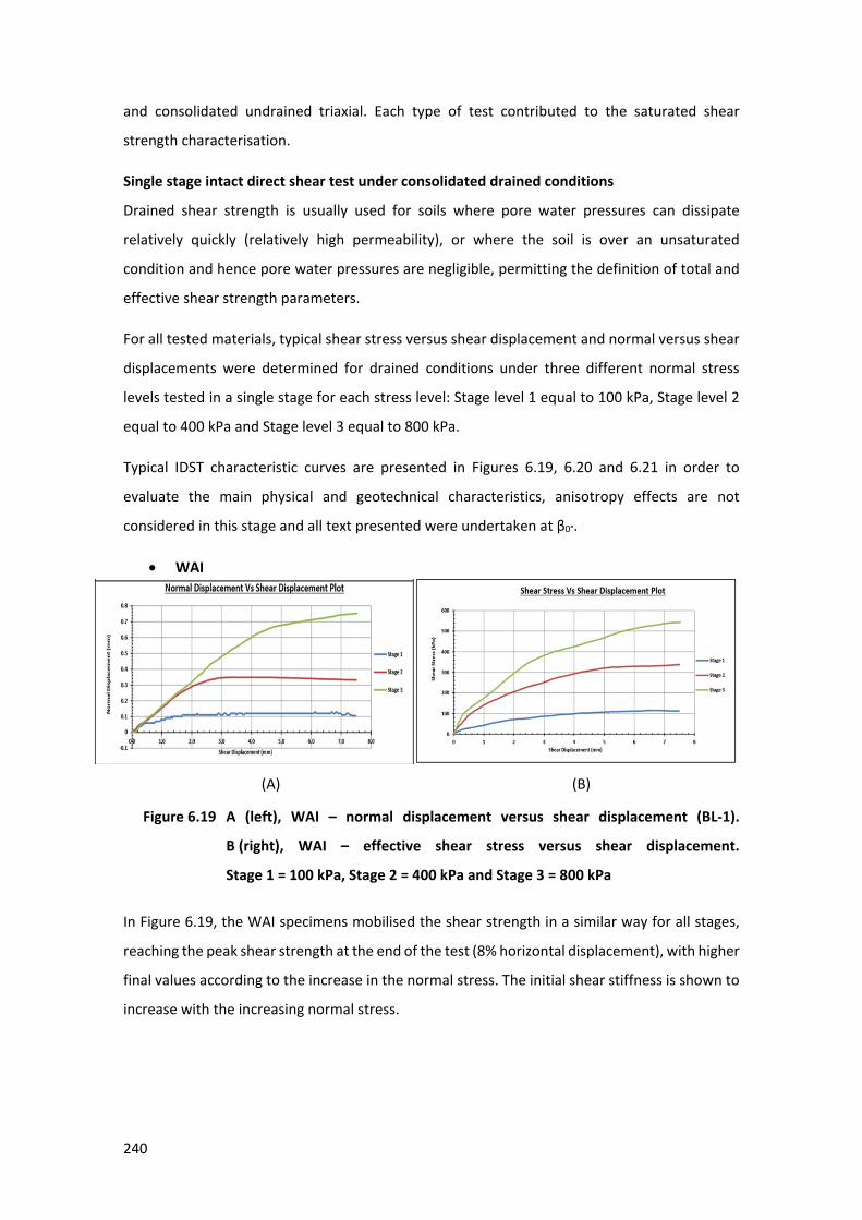
240
and consolidated undrained triaxial. Each type of test contributed to the saturated shear
strength characterisation.
Single stage intact direct shear test under consolidated drained conditions
Drained shear strength is usually used for soils where pore water pressures can dissipate
relatively quickly (relatively high permeability), or where the soil is over an unsaturated
condition and hence pore water pressures are negligible, permitting the definition of total and
effective shear strength parameters.
For all tested materials, typical shear stress versus shear displacement and normal versus shear
displacements were determined for drained conditions under three different normal stress
levels tested in a single stage for each stress level: Stage level 1 equal to 100 kPa, Stage level 2
equal to 400 kPa and Stage level 3 equal to 800 kPa.
Typical IDST characteristic curves are presented in Figures 6.19, 6.20 and 6.21 in order to
evaluate the main physical and geotechnical characteristics, anisotropy effects are not
considered in this stage and all text presented were undertaken at β0°.
• WAI
(A) (B)
69 Figure 6.19 A (left), WAI – normal displacement versus shear displacement (BL-1).
B (right), WAI – effective shear stress versus shear displacement.
Stage 1 = 100 kPa, Stage 2 = 400 kPa and Stage 3 = 800 kPa
In Figure 6.19, the WAI specimens mobilised the shear strength in a similar way for all stages,
reaching the peak shear strength at the end of the test (8% horizontal displacement), with higher
final values according to the increase in the normal stress. The initial shear stiffness is shown to
increase with the increasing normal stress.
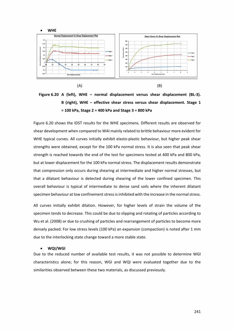
241
• WHE
(A) (B)
70 Figure 6.20 A (left), WHE – normal displacement versus shear displacement (BL-3).
B (right), WHE – effective shear stress versus shear displacement. Stage 1
= 100 kPa, Stage 2 = 400 kPa and Stage 3 = 800 kPa
Figure 6.20 shows the IDST results for the WHE specimens. Different results are observed for
shear development when compared to WAI mainly related to brittle behaviour more evident for
WHE typical curves. All curves initially exhibit elasto-plastic behaviour, but higher peak shear
strengths were obtained, except for the 100 kPa normal stress. It is also seen that peak shear
strength is reached towards the end of the test for specimens tested at 400 kPa and 800 kPa,
but at lower displacement for the 100 kPa normal stress. The displacement results demonstrate
that compression only occurs during shearing at intermediate and higher normal stresses, but
that a dilatant behaviour is detected during shearing of the lower confined specimen. This
overall behaviour is typical of intermediate to dense sand soils where the inherent dilatant
specimen behaviour at low confinement stress is inhibited with the increase in the normal stress.
All curves initially exhibit dilation. However, for higher levels of strain the volume of the
specimen tends to decrease. This could be due to slipping and rotating of particles according to
Wu et al. (2008) or due to crushing of particles and rearrangement of particles to become more
densely packed. For low stress levels (100 kPa) an expansion (compaction) is noted after 1 mm
due to the interlocking state change toward a more stable state.
• WQI/WGI Due to the reduced number of available test results, it was not possible to determine WGI
characteristics alone; for this reason, WGI and WQI were evaluated together due to the
similarities observed between these two materials, as discussed previously.
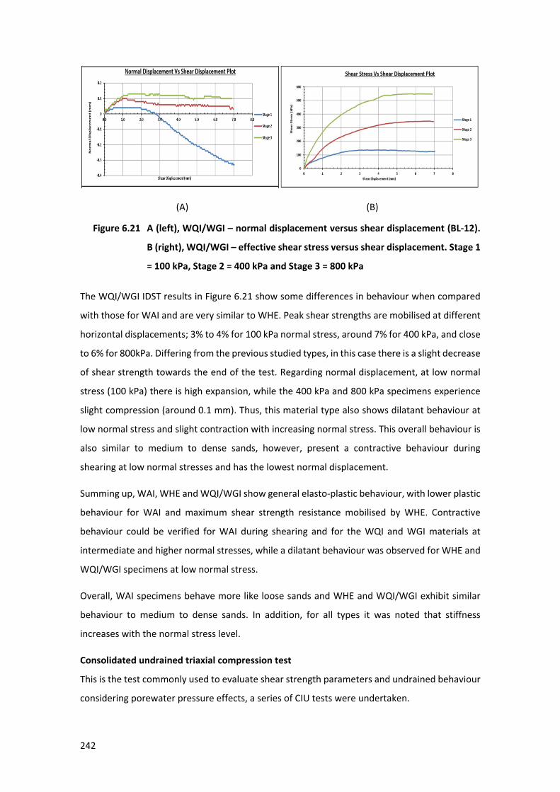
242
(A) (B)
71 Figure 6.21 A (left), WQI/WGI – normal displacement versus shear displacement (BL-12).
B (right), WQI/WGI – effective shear stress versus shear displacement. Stage 1
= 100 kPa, Stage 2 = 400 kPa and Stage 3 = 800 kPa
The WQI/WGI IDST results in Figure 6.21 show some differences in behaviour when compared
with those for WAI and are very similar to WHE. Peak shear strengths are mobilised at different
horizontal displacements; 3% to 4% for 100 kPa normal stress, around 7% for 400 kPa, and close
to 6% for 800kPa. Differing from the previous studied types, in this case there is a slight decrease
of shear strength towards the end of the test. Regarding normal displacement, at low normal
stress (100 kPa) there is high expansion, while the 400 kPa and 800 kPa specimens experience
slight compression (around 0.1 mm). Thus, this material type also shows dilatant behaviour at
low normal stress and slight contraction with increasing normal stress. This overall behaviour is
also similar to medium to dense sands, however, present a contractive behaviour during
shearing at low normal stresses and has the lowest normal displacement.
Summing up, WAI, WHE and WQI/WGI show general elasto-plastic behaviour, with lower plastic
behaviour for WAI and maximum shear strength resistance mobilised by WHE. Contractive
behaviour could be verified for WAI during shearing and for the WQI and WGI materials at
intermediate and higher normal stresses, while a dilatant behaviour was observed for WHE and
WQI/WGI specimens at low normal stress.
Overall, WAI specimens behave more like loose sands and WHE and WQI/WGI exhibit similar
behaviour to medium to dense sands. In addition, for all types it was noted that stiffness
increases with the normal stress level.
Consolidated undrained triaxial compression test
This is the test commonly used to evaluate shear strength parameters and undrained behaviour
considering porewater pressure effects, a series of CIU tests were undertaken.
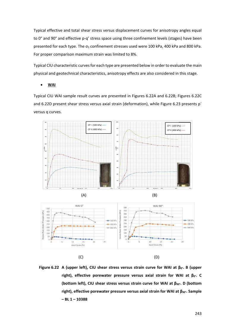
243
Typical effective and total shear stress versus displacement curves for anisotropy angles equal
to 0° and 90° and effective p-q’ stress space using three confinement levels (stages) have been
presented for each type. The σ3 confinement stresses used were 100 kPa, 400 kPa and 800 kPa.
For proper comparison maximum strain was limited to 8%.
Typical CIU characteristic curves for each type are presented below in order to evaluate the main
physical and geotechnical characteristics, anisotropy effects are also considered in this stage.
• WAI
Typical CIU WAI sample result curves are presented in Figures 6.22A and 6.22B; Figures 6.22C
and 6.22D present shear stress versus axial strain (deformation), while Figure 6.23 presents p´
versus q curves.
(A) (B)
(C) (D)
72 Figure 6.22 A (upper left), CIU shear stress versus strain curve for WAI at β0°. B (upper
right), effective porewater pressure versus axial strain for WAI at β0°. C
(bottom left), CIU shear stress versus strain curve for WAI at β90°. D (bottom
right), effective porewater pressure versus axial strain for WAI at β90°. Sample
– BL 1 – 10388
CP I (100 kPa) -----
CP II (400 kPa) -----
CP I (100 kPa) -----
CP II (400 kPa) -----
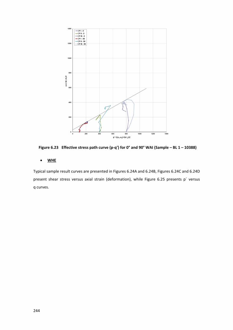
244
73 Figure 6.23 Effective stress path curve (p-q’) for 0° and 90° WAI (Sample – BL 1 – 10388)
• WHE
Typical sample result curves are presented in Figures 6.24A and 6.24B, Figures 6.24C and 6.24D
present shear stress versus axial strain (deformation), while Figure 6.25 presents p´ versus
q curves.
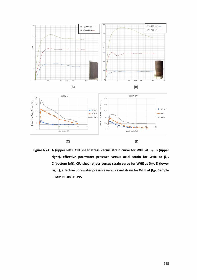
245
(A) (B)
(C) (D)
74 Figure 6.24 A (upper left), CIU shear stress versus strain curve for WHE at β0°. B (upper
right), effective porewater pressure versus axial strain for WHE at β0°.
C (bottom left), CIU shear stress versus strain curve for WHE at β90°. D (lower
right), effective porewater pressure versus axial strain for WHE at β90°. Sample
– TAM BL-08 -10395
CP I (100 kPa) -----
CP II (400 kPa) -----
CP I (100 kPa) -----
CP II (400 kPa) -----
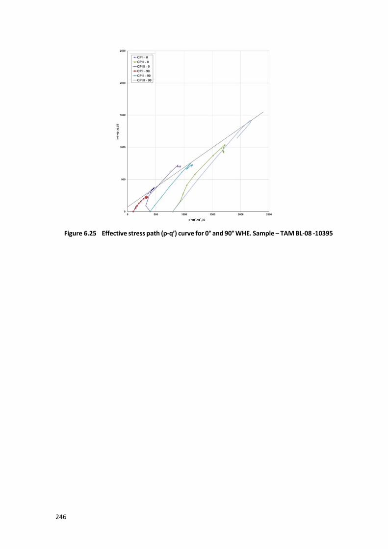
246
75 Figure 6.25 Effective stress path (p-q’) curve for 0° and 90° WHE. Sample – TAM BL-08 -10395
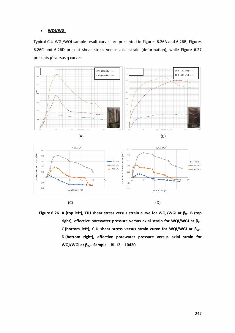
247
• WQI/WGI
Typical CIU WGI/WQI sample result curves are presented in Figures 6.26A and 6.26B; Figures
6.26C and 6.26D present shear stress versus axial strain (deformation), while Figure 6.27
presents p´ versus q curves.
(A) (B)
(C) (D)
76 Figure 6.26 A (top left), CIU shear stress versus strain curve for WQI/WGI at β0°. B (top
right), effective porewater pressure versus axial strain for WQI/WGI at β0°.
C (bottom left), CIU shear stress versus strain curve for WQI/WGI at β90°.
D (bottom right), effective porewater pressure versus axial strain for
WQI/WGI at β90°. Sample – BL 12 – 10420
CP I (100 kPa) -----
CP II (400 kPa) -----
CP I (100 kPa) -----
CP II (400 kPa) -----
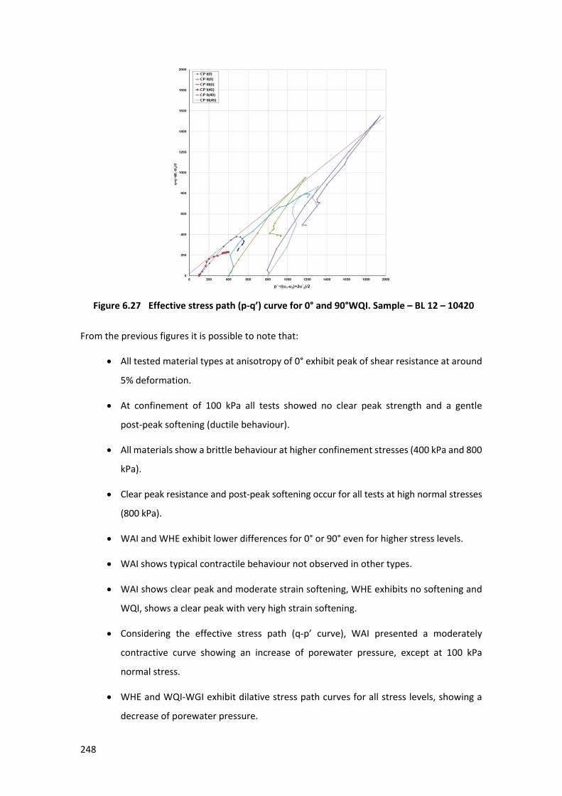
248
77 Figure 6.27 Effective stress path (p-q’) curve for 0° and 90°WQI. Sample – BL 12 – 10420
From the previous figures it is possible to note that:
• All tested material types at anisotropy of 0° exhibit peak of shear resistance at around
5% deformation.
• At confinement of 100 kPa all tests showed no clear peak strength and a gentle
post-peak softening (ductile behaviour).
• All materials show a brittle behaviour at higher confinement stresses (400 kPa and 800
kPa).
• Clear peak resistance and post-peak softening occur for all tests at high normal stresses
(800 kPa).
• WAI and WHE exhibit lower differences for 0° or 90° even for higher stress levels.
• WAI shows typical contractile behaviour not observed in other types.
• WAI shows clear peak and moderate strain softening, WHE exhibits no softening and
WQI, shows a clear peak with very high strain softening.
• Considering the effective stress path (q-p’ curve), WAI presented a moderately
contractive curve showing an increase of porewater pressure, except at 100 kPa
normal stress.
• WHE and WQI-WGI exhibit dilative stress path curves for all stress levels, showing a
decrease of porewater pressure.
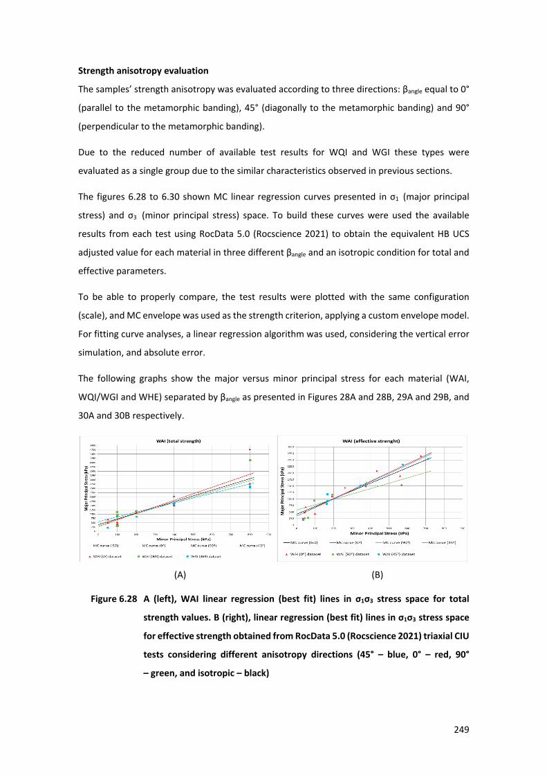
249
Strength anisotropy evaluation
The samples’ strength anisotropy was evaluated according to three directions: βangle equal to 0°
(parallel to the metamorphic banding), 45° (diagonally to the metamorphic banding) and 90°
(perpendicular to the metamorphic banding).
Due to the reduced number of available test results for WQI and WGI these types were
evaluated as a single group due to the similar characteristics observed in previous sections.
The figures 6.28 to 6.30 shown MC linear regression curves presented in σ1 (major principal
stress) and σ3 (minor principal stress) space. To build these curves were used the available
results from each test using RocData 5.0 (Rocscience 2021) to obtain the equivalent HB UCS
adjusted value for each material in three different βangle and an isotropic condition for total and
effective parameters.
To be able to properly compare, the test results were plotted with the same configuration
(scale), and MC envelope was used as the strength criterion, applying a custom envelope model.
For fitting curve analyses, a linear regression algorithm was used, considering the vertical error
simulation, and absolute error.
The following graphs show the major versus minor principal stress for each material (WAI,
WQI/WGI and WHE) separated by βangle as presented in Figures 28A and 28B, 29A and 29B, and
30A and 30B respectively.
(A) (B)
78 Figure 6.28 A (left), WAI linear regression (best fit) lines in σ1σ3 stress space for total
strength values. B (right), linear regression (best fit) lines in σ1σ3 stress space
for effective strength obtained from RocData 5.0 (Rocscience 2021) triaxial CIU
tests considering different anisotropy directions (45° – blue, 0° – red, 90°
– green, and isotropic – black)
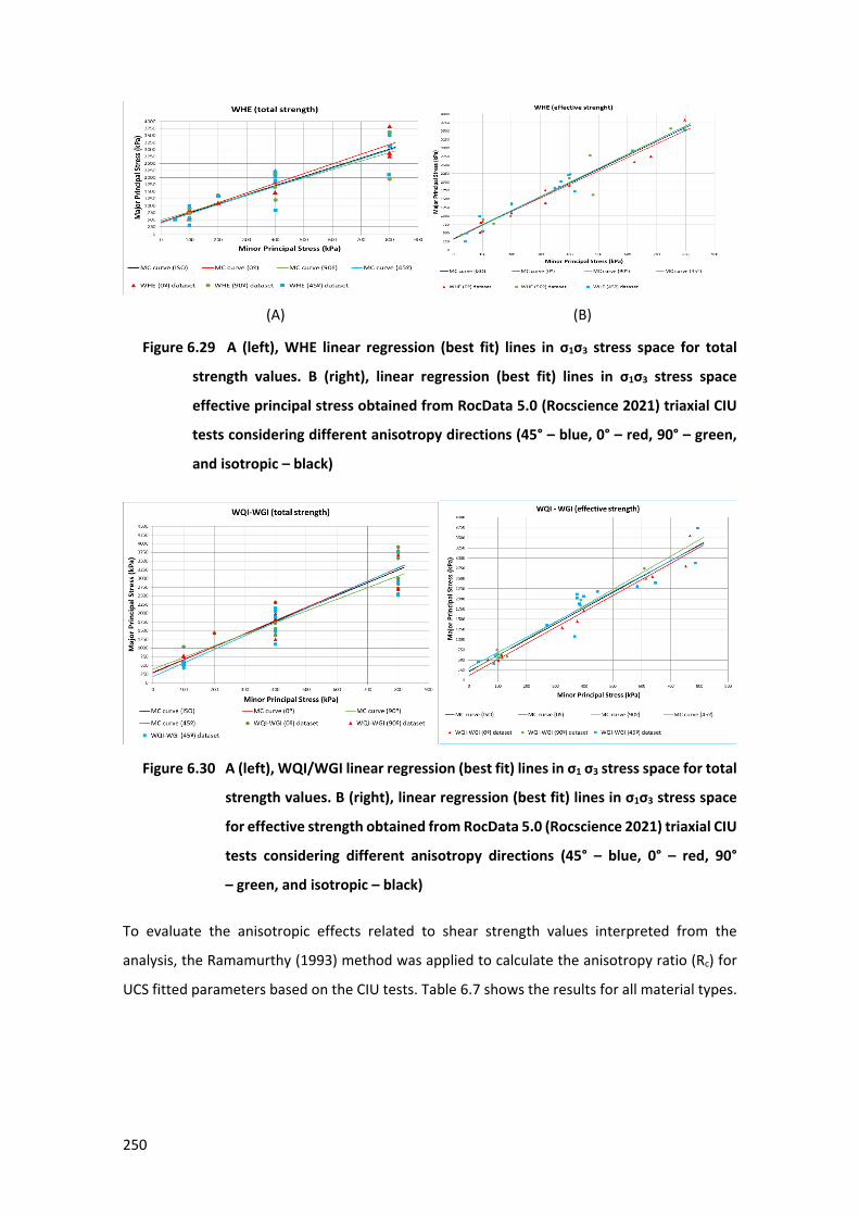
250
(A) (B)
79 Figure 6.29 A (left), WHE linear regression (best fit) lines in σ1σ3 stress space for total
strength values. B (right), linear regression (best fit) lines in σ1σ3 stress space
effective principal stress obtained from RocData 5.0 (Rocscience 2021) triaxial CIU
tests considering different anisotropy directions (45° – blue, 0° – red, 90° – green,
and isotropic – black)
80 Figure 6.30 A (left), WQI/WGI linear regression (best fit) lines in σ1 σ3 stress space for total
strength values. B (right), linear regression (best fit) lines in σ1σ3 stress space
for effective strength obtained from RocData 5.0 (Rocscience 2021) triaxial CIU
tests considering different anisotropy directions (45° – blue, 0° – red, 90°
– green, and isotropic – black)
To evaluate the anisotropic effects related to shear strength values interpreted from the
analysis, the Ramamurthy (1993) method was applied to calculate the anisotropy ratio (Rc) for
UCS fitted parameters based on the CIU tests. Table 6.7 shows the results for all material types.
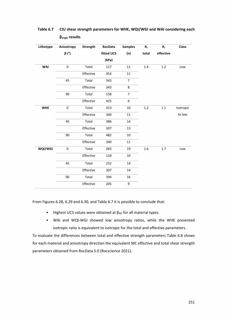
251
21 Table 6.7 CIU shear strength parameters for WHE, WQI/WGI and WAI considering each
βangle results
Lithotype Anisotropy
β (°)
Strength RocData
fitted UCS
(kPa)
Samples
(n)
Rc
total
Rc
effective
Class
WAI 0 Total 117 11 1.4 1.2 Low
Effective 354 11
45 Total 343 7
Effective 343 8
90 Total 158 7
Effective 425 6
WHE 0 Total 413 10 1.2 1.1 Isotropic
to low
Effective 340 11
45 Total 386 14
Effective 307 13
90 Total 482 10
Effective 340 11
WQI/WGI 0 Total 283 19 1.6 1.7 Low
Effective 118 10
45 Total 252 14
Effective 307 14
90 Total 394 16
Effective 205 9
From Figures 6.28, 6.29 and 6.30, and Table 6.7 it is possible to conclude that:
• Highest UCS values were obtained at β90° for all material types.
• WAI and WQI-WGI showed low anisotropy ratios, while the WHE presented
isotropic ratio is equivalent to isotropic for the total and effective parameters.
To evaluate the differences between total and effective strength parameters Table 6.8 shows
for each material and anisotropy direction the equivalent MC effective and total shear strength
parameters obtained from RocData 5.0 (Rocscience 2021).
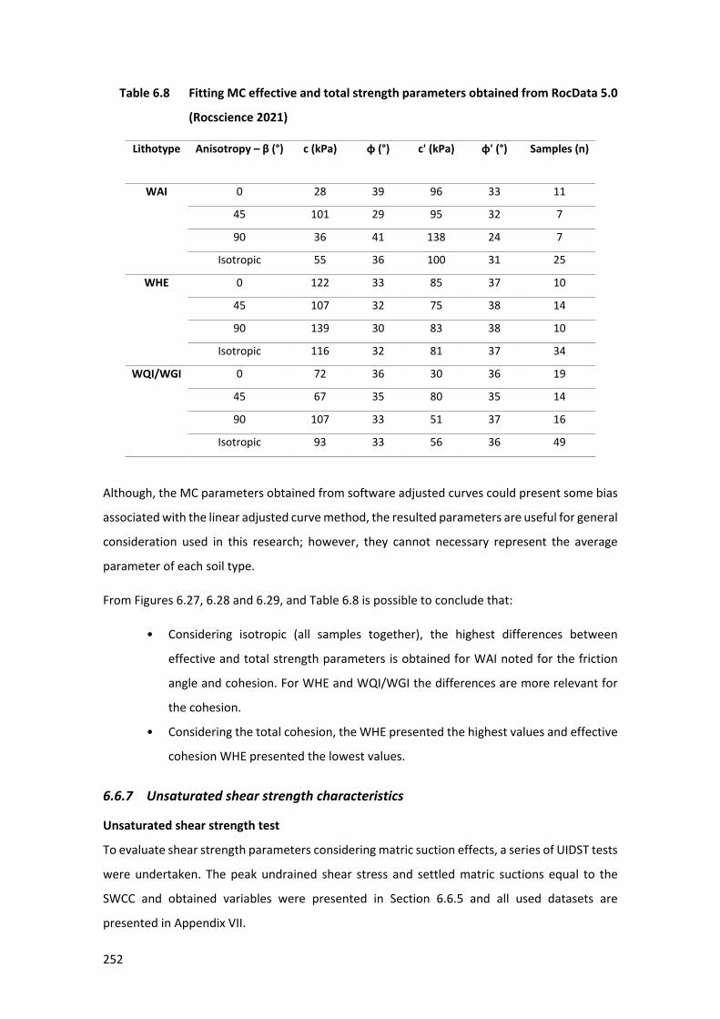
252
22 Table 6.8 Fitting MC effective and total strength parameters obtained from RocData 5.0
(Rocscience 2021)
Lithotype Anisotropy – β (°) c (kPa) ɸ (°) c' (kPa) ɸ' (°) Samples (n)
WAI 0 28 39 96 33 11
45 101 29 95 32 7
90 36 41 138 24 7
Isotropic 55 36 100 31 25
WHE 0 122 33 85 37 10
45 107 32 75 38 14
90 139 30 83 38 10
Isotropic 116 32 81 37 34
WQI/WGI 0 72 36 30 36 19
45 67 35 80 35 14
90 107 33 51 37 16
Isotropic 93 33 56 36 49
Although, the MC parameters obtained from software adjusted curves could present some bias
associated with the linear adjusted curve method, the resulted parameters are useful for general
consideration used in this research; however, they cannot necessary represent the average
parameter of each soil type.
From Figures 6.27, 6.28 and 6.29, and Table 6.8 is possible to conclude that:
• Considering isotropic (all samples together), the highest differences between
effective and total strength parameters is obtained for WAI noted for the friction
angle and cohesion. For WHE and WQI/WGI the differences are more relevant for
the cohesion.
• Considering the total cohesion, the WHE presented the highest values and effective
cohesion WHE presented the lowest values.
6.6.7 Unsaturated shear strength characteristics
Unsaturated shear strength test
To evaluate shear strength parameters considering matric suction effects, a series of UIDST tests
were undertaken. The peak undrained shear stress and settled matric suctions equal to the
SWCC and obtained variables were presented in Section 6.6.5 and all used datasets are
presented in Appendix VII.
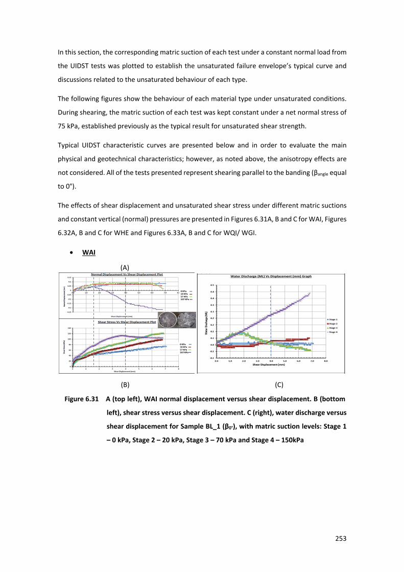
253
In this section, the corresponding matric suction of each test under a constant normal load from
the UIDST tests was plotted to establish the unsaturated failure envelope’s typical curve and
discussions related to the unsaturated behaviour of each type.
The following figures show the behaviour of each material type under unsaturated conditions.
During shearing, the matric suction of each test was kept constant under a net normal stress of
75 kPa, established previously as the typical result for unsaturated shear strength.
Typical UIDST characteristic curves are presented below and in order to evaluate the main
physical and geotechnical characteristics; however, as noted above, the anisotropy effects are
not considered. All of the tests presented represent shearing parallel to the banding (βangle equal
to 0°).
The effects of shear displacement and unsaturated shear stress under different matric suctions
and constant vertical (normal) pressures are presented in Figures 6.31A, B and C for WAI, Figures
6.32A, B and C for WHE and Figures 6.33A, B and C for WQI/ WGI.
• WAI
(A)
(B) (C)
8 Figure 6.31 A (top left), WAI normal displacement versus shear displacement. B (bottom
left), shear stress versus shear displacement. C (right), water discharge versus
shear displacement for Sample BL_1 (β0°), with matric suction levels: Stage 1
– 0 kPa, Stage 2 – 20 kPa, Stage 3 – 70 kPa and Stage 4 – 150kPa
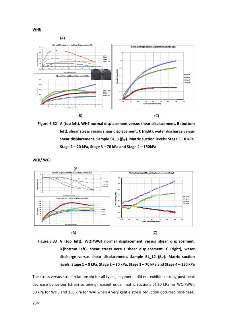
254
WHE
(A)
(B) (C)
82 Figure 6.32 A (top left), WHE normal displacement versus shear displacement. B (bottom
left), shear stress versus shear displacement. C (right), water discharge versus
shear displacement. Sample BL_3 (β0°). Matric suction levels: Stage 1– 0 kPa,
Stage 2 – 20 kPa, Stage 3 – 70 kPa and Stage 4 – 150kPa
WQI/ WGI
(A)
(B) (C)
83 Figure 6.33 A (top left), WQI/WGI normal displacement versus shear displacement.
B (bottom left), shear stress versus shear displacement. C (right), water
discharge versus shear displacement. Sample BL_12 (β0°). Matric suction
levels: Stage 1 – 0 kPa, Stage 2 – 20 kPa, Stage 3 – 70 kPa and Stage 4 – 150 kPa
The stress versus strain relationship for all types, in general, did not exhibit a strong post-peak
decrease behaviour (strain softening), except under matric suctions of 20 kPa for WQI/WGI,
30 kPa for WHE and 150 kPa for WAI when a very gentle stress reduction occurred post-peak.
255
The volume change/normal displacement associated with each test exhibited dilatation for all
WHE curves, and contraction at the beginning and subsequent expansion for all WQI/WGI
curves, and expansion for WAI at the low suction levels and contraction for the highest suction
level (150 kPa).
As expected, high permeable material such as the WHE specimen showed intense discharge up
to 2 mm of shear displacement, after which there was a reduction in the discharge intensity. For
WAI the lower suction levels (0 and 20 kPa) showed no discharge, after which higher suction
levels resulted in a constant discharge rate until 1.5 mm shear displacement when material
stopped draining at a suction level of 70 kPa and started wetting, or still kept discharging until
the end of the test when the suction level was 150 kPa.
The same occurs with WQI/WGI, which presented no discharge for a suction level of 0 kPa; for
a suction level of 20 kPa, it discharged until 1 mm of shear displacement and from that point it
started wetting, with no equilibrium until the end of the test. In contrast, for a suction level of
70 kPa, it exhibited a wetting process up to 1 mm of shear displacement and from that point
onwards a constant discharge rate until equilibrium was reached after 4 mm displacement. At a
suction level of 150 kPa, it started with fast discharge until 4 mm displacement and from this
point onward it continued with a constant discharge rate with no equilibrium.
Figures 6.31, 6.32 and 6.33 show that peak shear strength increases as matric suction increases
in nonlinear form. Although the well-known shear strength equation developed by Fredlund et
al. (1978) is linear, many experimental results from Gan et al. (1988b), Escario & Jucá (1989) and
Wheeler & Sivakumar (1992) show nonlinear variations of shear strength with respect to matric
suction when tested over a wide range of matric suction.
It is noticed that all lines tend to curve as the matric suction approaches a specified value. This
value was found to be within the range of 50 kPa to 250 kPa for WAI, 40 kPa to 100 kPa for WHE,
and 20 kPa to 70 kPa for WQI-WGI, respectively. This could be associated with studies carried
out by Fredlund & Rahardjo (1993) concluded that this value corresponds to the AEV of the soil.
It is clear from Figures 6.31, 6.32 and 6.33 that envelope lines are almost parallel, and that for
higher values of matric suction there is an increment in the shear strength for the first part of
the curves.
256
6.7 DISCUSSION
Considering each completely weathered BIF, based on USCS soil classification, the WAI is
characterised as fine sand silt, with medium plasticity even with a low clay percentage (less than
5%) in which kaolinite and gibbsite (weathered minerals), are responsible for a low activity
behaviour and the uniform PSD that typically results in a low permeability (6.6×10⁻⁶ cm/s).
The presence of kaolinite and gibbsite are also responsible for the lowest shear strength and low
anisotropy ratio. Heterogeneity is defined by interlayers of silt clayish and hematite minerals,
resulting in the highest mineralogical hardness contrast for the completely weathered BIF.
The soil classification of WHE is as a sandy-silt material, with low plasticity and characteristics of
non-cohesive soils as noted in Section 6.6.6. Heterogeneity is defined by granular and micro-
plates of hematite with variable visual total porosity layers resulting in a high permeability of
3.1×10⁻⁴ cm/s. Due to this high Øb, mineral orientation seems to have a secondary importance in
defining anisotropy, resulting in an isotropic to low anisotropy ratio. Different to other
weathered itabirites the WHE genesis is associated with mimetic supergenic process as defined
by Morris (2002 and 2002a); arguing that the higher Øb levels are associated with previous non-
iron layers that have been totally leached, generating highly porous layers (partially filled by iron
oxides and hydroxides near the surface). This modifies the original bimodal minerology (non-
iron and iron bands), forming a monomineralic hematitic material, in which the original
heterogeneity was obliterated by layers of iron minerals with variable Øb and a very low strength
when compared to the parent rock fresh itabirites.
Secondarily, the lattice weathering (Morris 2002 and 2002a), induces iron oxidation and
reprecipitation as iron oxide or hydroxy cementing the pores and increasing the shear strength.
WQI is classified as silt-sand with gravel material with a non-uniform size distribution and
permeability of 9.1×10⁻⁵ cm/s. The heterogeneity defined by the partial leaching is clearly visible
and is defined by iron layers (higher ρb and lower Øb) and quartz layers (lower ρb and higher Øb).
In general, this type presents a typical granoblastic crystal orientation; however, the fabric did
not play an important role for shear strength results compared with non-oriented types. The
low anisotropic ratio obtained for this type is mainly defined by the mineral composition (band
thickness), iron cementation and Øb that seems to equally contribute to this behaviour.
WGI differs from WQI due to the higher presence of goethite and ochreous goethite cemented
bands. Additionally, the WQI presents higher Øb when compared with WGI induced by iron oxide
and mainly hydroxide cementation. For WGI, even with the typical heterogeneity preserved, this
257
material presents low anisotropy ratio and higher shear strength due to cementation compared
with the WQI.
Completely weathered BIF presents, in general, a very high ρb and a well-structured high visual
total porosity mineral skeleton; and a relatively high shear strength when compared with low
dense sand silt soils as sandstones or limestones, as postulated by Costa (2009) and Martin &
Stacey (2018). Otherwise, BIF with lower ρb and high total porosity (e.g. WAI) represents the
weaker types with lower shear strength seams normally associated with the presence of clay
minerals (gibbsite and kaolinite) as resulted from weathering.
Saturated tests indicate that WHE, WQI and WGI behave as a brittle, dense sand silt soils above
a 400 kPa stress level, and below this level they behave more like ductile, loose sand silt soils.
This behaviour could in part be attributed to the high particle densities typical of BIF. However,
the bulk density is in turn partially controlled for the most part by the total porosity, although
not enough to fully control this behaviour. An additional petrophysical characteristic that should
influence weak BIF behaviour is the mineral composition associated with each material type
(quartz, gibbsite, kaolinite and different iron oxides) and, to a lesser extent the fabric (mineral
orientation).
The loose sand silt behaviour below 400 kPa results in slip between particles where only the
friction between the crystals must be overcome. As the stress increases, the samples show a
continuous decrease in volume, i.e. contraction. Conversely, dense sand silts interlocking
between the particles will require additional effort to allow shearing, requiring an increase in
(dilatancy) volume for it to occur. Dense sand reaches a maximum shear stress (peak) then starts
softening rapidly reaching a residual constant shear stress value.
In summary, for individual layers in the BIF units, mineral composition, total porosity, and
associated fabric are essential components that influence the behaviour and shear strength
parameters. An example of this is that thin layers of clay minerals that could exhibit matric
suction values from tens to hundreds of kilopascals (kPa), e.g. in WAI. When comparing matric
suction effects in weathered BIF units, WGI also involves a high percentage of clay size mineral
content (maximum of 10%). However, it does not exhibit the important content of clay minerals
and does not exhibit high matric suction effects. On the other hand, WAI, even with low (3%
average) clay minerals content, shows the highest matric suction effects. This can be attributed
not only to the clay percentage, but also to clay activity as the WAI clay fraction is mainly
comprised of kaolinite and gibbsite (low activity minerals), whereas the WGI clay fraction is
comprised of goethite and ochreous goethite. In addition to the clay percentage content the
258
contribution of clay activity to the matric suction must be considered as the main clay mineral
(kaolinite) is a non-active clay mineral.
The compositional metamorphic banding defines a heterogeneity easily recognised in all highly
to completely weathered BIF and induces a low anisotropic behaviour, as obtained from CIU
tests shown in Table 6.7. From this table WHE shows isotropic to low anisotropic ratio and the
heterogeneity is defined by layers of sandy-silt iron minerals with higher visual total porosity,
interlayered with sand silt iron mineral bands with low visual total porosity. WAI and WQI/WGI
show a low anisotropy ratio and WAI are constituted of sandy-silt layers of iron minerals
interlayered with non-iron minerals silty-sand and varying in percentages of clay minerals
(kaolinite and gibbsite). WQI is characterised by silty-sand with gravel iron mineral layers that
have a lower visual total porosity interlayered with bands of silty-sand iron minerals and quartz
with higher Øb. WGI differs from WQI due to a higher percentage of iron hydroxide minerals and
gibbsite, with more pores filled (cemented), resulting in a relatively lower Øb. From this study,
WAI and WGI were considered as the lower Øb types (less than 15%) and WHE and WQI the
higher total porosity types (higher than 15%).
From the weathering, it is recognised that increases in total porosity and mineral alteration are
important changes that produce an effective softening of the original fresh rocks. For BIF, this
softening is produced by the partial or total leaching of non-iron minerals, mainly iron dolomite,
but also quartz; oxidation of iron minerals; and chemical alteration of amphibole and other
minerals. In extreme cases, the remaining iron oxidises, and non-iron bands (mainly quartz)
exhibit a high total porosity and low grain apparent cohesion (loss of contact between grains).
This results in a weak soil material that is occasionally cemented by secondary iron oxides and/or
hydroxides (WGI), which impose some additional strength due to the total porosity reduction.
These results outlined above generally agree with studies by Gupta & Rao (2001) for crystalline
rocks, Marques et al. (2010) for Australian and Brazilian metamorphic rocks and Leão et al.
(2017) for Brazilian phyllites.
The geological events responsible for the control of the total porosity are the low-grade regional
metamorphism (mainly for bedrock), supergene and hypogene events, and weathering.
Considering each event, the metamorphism promotes granuloblast texture, with small crystals
oriented according to banding. Supergene and hypogene events transformed the bedrock
crystalline phases of iron minerals (hematite, magnetite and martite), and partial or total
leaching of non-iron minerals (quartz and iron dolomite) providing a volumetric reduction which
is responsible for increased intergranular porosity (Pimenta 1992). Finally, the iron enrichment
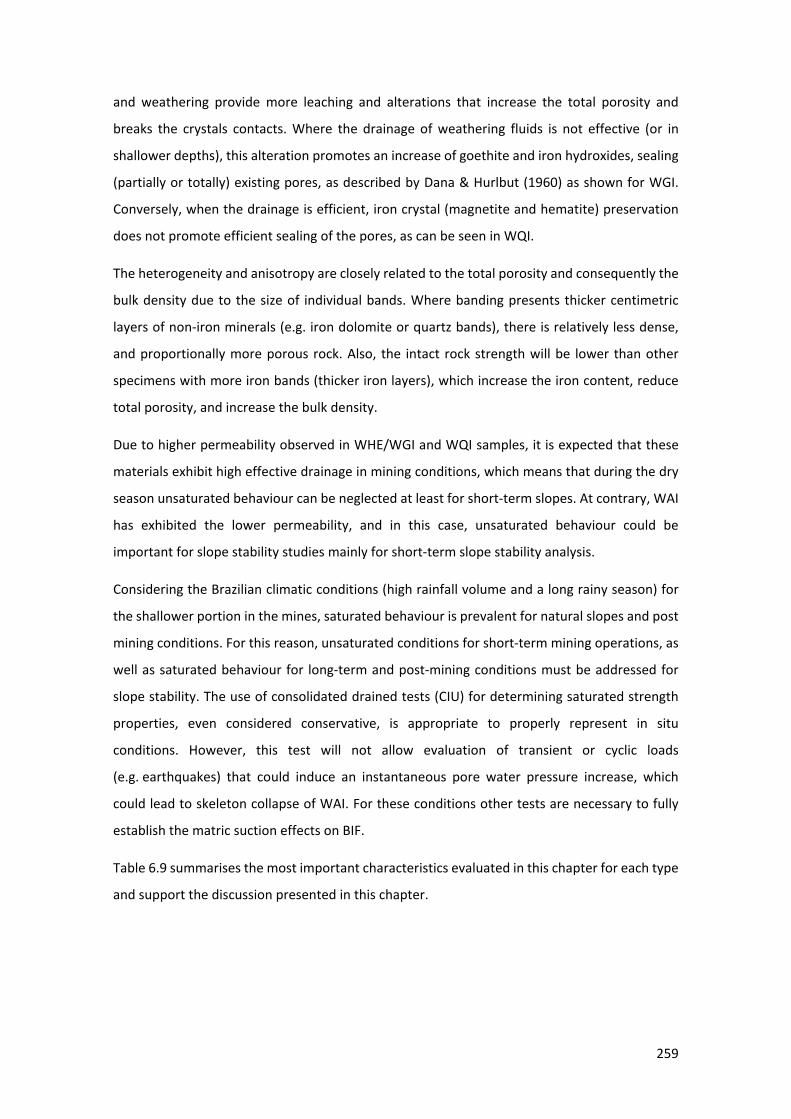
259
and weathering provide more leaching and alterations that increase the total porosity and
breaks the crystals contacts. Where the drainage of weathering fluids is not effective (or in
shallower depths), this alteration promotes an increase of goethite and iron hydroxides, sealing
(partially or totally) existing pores, as described by Dana & Hurlbut (1960) as shown for WGI.
Conversely, when the drainage is efficient, iron crystal (magnetite and hematite) preservation
does not promote efficient sealing of the pores, as can be seen in WQI.
The heterogeneity and anisotropy are closely related to the total porosity and consequently the
bulk density due to the size of individual bands. Where banding presents thicker centimetric
layers of non-iron minerals (e.g. iron dolomite or quartz bands), there is relatively less dense,
and proportionally more porous rock. Also, the intact rock strength will be lower than other
specimens with more iron bands (thicker iron layers), which increase the iron content, reduce
total porosity, and increase the bulk density.
Due to higher permeability observed in WHE/WGI and WQI samples, it is expected that these
materials exhibit high effective drainage in mining conditions, which means that during the dry
season unsaturated behaviour can be neglected at least for short-term slopes. At contrary, WAI
has exhibited the lower permeability, and in this case, unsaturated behaviour could be
important for slope stability studies mainly for short-term slope stability analysis.
Considering the Brazilian climatic conditions (high rainfall volume and a long rainy season) for
the shallower portion in the mines, saturated behaviour is prevalent for natural slopes and post
mining conditions. For this reason, unsaturated conditions for short-term mining operations, as
well as saturated behaviour for long-term and post-mining conditions must be addressed for
slope stability. The use of consolidated drained tests (CIU) for determining saturated strength
properties, even considered conservative, is appropriate to properly represent in situ
conditions. However, this test will not allow evaluation of transient or cyclic loads
(e.g. earthquakes) that could induce an instantaneous pore water pressure increase, which
could lead to skeleton collapse of WAI. For these conditions other tests are necessary to fully
establish the matric suction effects on BIF.
Table 6.9 summarises the most important characteristics evaluated in this chapter for each type
and support the discussion presented in this chapter.
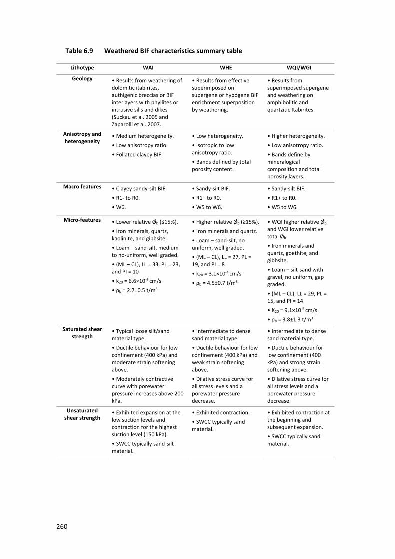
260
23 Table 6.9 Weathered BIF characteristics summary table
Lithotype WAI WHE WQI/WGI
Geology • Results from weathering of dolomitic itabirites, authigenic breccias or BIF interlayers with phyllites or intrusive sills and dikes (Suckau et al. 2005 and Zaparolli et al. 2007.
• Results from effective superimposed on supergene or hypogene BIF enrichment superposition by weathering.
• Results from superimposed supergene and weathering on amphibolitic and quartzitic Itabirites.
Anisotropy and heterogeneity
• Medium heterogeneity. • Low anisotropy ratio. • Foliated clayey BIF.
• Low heterogeneity. • Isotropic to low anisotropy ratio. • Bands defined by total porosity content.
• Higher heterogeneity. • Low anisotropy ratio. • Bands define by mineralogical composition and total porosity layers.
Macro features • Clayey sandy-silt BIF. • R1- to R0. • W6.
• Sandy-silt BIF. • R1+ to R0. • W5 to W6.
• Sandy-silt BIF. • R1+ to R0. • W5 to W6.
Micro-features • Lower relative Øb (≤15%). • Iron minerals, quartz, kaolinite, and gibbsite. • Loam – sand-silt, medium to no-uniform, well graded. • (ML – CL), LL = 33, PL = 23, and PI = 10 • k20 = 6.6×10⁻⁶ cm/s • ρb = 2.7±0.5 t/m3
• Higher relative Øb (≥15%). • Iron minerals and quartz. • Loam – sand-silt, no uniform, well graded. • (ML – CL), LL = 27, PL = 19, and PI = 8 • k20 = 3.1×10⁻⁴ cm/s • ρb = 4.5±0.7 t/m3
• WQI higher relative Øb and WGI lower relative total Øb. • Iron minerals and quartz, goethite, and gibbsite. • Loam – silt-sand with gravel, no uniform, gap graded. • (ML – CL), LL = 29, PL = 15, and PI = 14 • K20 = 9.1×10⁻⁵ cm/s • ρb = 3.8±1.3 t/m3
Saturated shear strength
• Typical loose silt/sand material type. • Ductile behaviour for low confinement (400 kPa) and moderate strain softening above. • Moderately contractive curve with porewater pressure increases above 200 kPa.
• Intermediate to dense sand material type. • Ductile behaviour for low confinement (400 kPa) and weak strain softening above. • Dilative stress curve for all stress levels and a porewater pressure decrease.
• Intermediate to dense sand material type. • Ductile behaviour for low confinement (400 kPa) and strong strain softening above. • Dilative stress curve for all stress levels and a porewater pressure decrease.
Unsaturated shear strength
• Exhibited expansion at the low suction levels and contraction for the highest suction level (150 kPa). • SWCC typically sand-silt material.
• Exhibited contraction. • SWCC typically sand material.
• Exhibited contraction at the beginning and subsequent expansion. • SWCC typically sand material.
261
6.8 CONCLUSION
The use of combined soil terminology and characterisation is appropriated for soil-like BIF
materials similar to the types evaluated in this chapter. The classification proposed for these
types ranges from very stiff to hard clay, through extremely weak to very weak rocks that ranges
from highly (W4), to completely weathered (W5) rocks and to residual soils (W6). These
materials, in general, behave like soils and follow soil mechanical approaches, and inherent relict
anisotropy of the original intact rock may have some influence on slope stability.
From the original fresh parent BIF, mainly the supergenic leaching effectiveness and weathering
promotes alteration processes (oxidation and leaching) inducing a significant increase in voids
and resulting in a reduction of the ρb for some types, e.g. WQI and WAI. Conversely, for WHE
and WGI, the same process produces the same changes but with iron minerals reconcentration
(iron enrichment) resulting in a relative bulk density increase. The physical characteristics
variation noted for each type is attributed to a superposition of the tectonic, supergene and
hypogene events occurred before weathering that contribute to the formation of multiple BIF
materials. This superposition is reduced in depth as supergenic enrichment and weathering
reduce their influence in depth.
However, for shallower depths, these changes are not restricted to void increase or ρb variations.
These multiple weathering processes also impose a mineral alteration, increase in clay minerals
(mainly gibbsite and kaolinite), resulting in a relative plasticity increase inducing some negative
porewater pressures (matric suction), as noted for WAI and in some extent to WGI. Also, for
WGI the iron minerals oxidation and hydration promote mineral alteration responsible for
cementation increase and a relatively higher shear strength for typical sand-silt materials with
low plasticity.
Close to surface, is characterising highly to completely weathered BIF as immature residual soils,
i.e. as materials which are formed in place from mineralogical changes, can properly describe
these BIF types. In general, all types studied exhibited distinct soil behaviours, but can be
grouped using USCS classification. The groups are characterised by the low (WQI, WGI and WHE)
to intermediate (WAI) plasticity index, and as sandy-silty soils, with clay and very low
permeability (WAI) and silt-sandy soils with gravel with low to moderate permeability (WQI, WGI
and WHE).
The original compositional metamorphic banding (noted at great depths) works as a preferential
path for all deleterious processes (weathering, supergene or hypogene) and defines anisotropic
characteristics for weathered BIF varieties. This anisotropy is defined for WQI by the alternation
262
of bands with quartz/goethite with high total porosity and bands of iron minerals with low total
porosity, which induces a low anisotropy ratio and high heterogeneity. Considering WGI, the
anisotropy is similar to WQI, and the shear strength increases due to iron oxide and hydroxide
cementation. For WHE, the anisotropy ratio can vary from an isotropic to low anisotropy and is
basically defined by the presence of pores layers. The compositional metamorphic banding is
less evident as the WHE is almost a monomineralic type and the heterogeneity is defined by the
alternation of bands with lower and higher total porosity.
For WAI, the anisotropy ratio is low, and the heterogeneity is defined by interlayers of quartz
and clay mineral bands with higher total porosity in contrast with iron mineral bands with lower
total porosity. For all BIF residual soils, the heterogeneity and anisotropy ratio are also controlled
by the thickness of these individual bands what is associated to sample scale effect.
Considering the heterogeneity and the anisotropy from these soils, mineralogy represents the
most important characteristic. However, the fabric, pores percentage and distribution, and bulk
density may contribute to the full understanding of the multiple behaviours of the weathered
BIF material, and better define the geological categorisation as an immature to residual soil.
Studies presented in this section show that highly to completely weathered BIF share some
common petrophysical characteristics representing dense sand silt materials with relatively high
shear strength parameters, compared to typical residual soils. However, single characteristics as
clay layers concentration for WAI, mineral orientation for WHE, clay layers concentration, and
pore layers concentration for WGI and WQI could induce local anisotropy effects and are
responsible for changes in the common behaviour, so resulting in multiple types.
For soil types with high total porosity as obtained for BIF residual soils, once the cohesion is
destroyed the load is transmitted to the soil skeleton, thereby mobilising the particle friction,
and this could induce sudden collapse during particle rearrangement. This collapse will occur
preferably at more pore layers or in the heterogeneity planes contacts as previously described
for Oolithic iron deposits by Cuccivillo & Coop (1997) and BIF by Martin & Stacey (2018). In this
matter, mineral and pore orientations can subsidiarily induce collapsed behaviour depending on
the stress level and material type. At low stress levels, the more isotropic types (WAI and WHE)
are more prone to ductile collapse than the low anisotropic materials for which the pore and
mineral orientations do not allow brittle failures since the fabric (skeleton) reorganisation redistributes the strain. As a result, the majority of evaluated failure envelopes for low
anisotropic materials are linear, showing no post-peak reduction. However, for isotropic types
263
(WHE) at higher stress levels a granular rearrangement can induce sudden collapse, as observed
in the brittle post-peak resistance loss (strain softening) in the majority of the test result curves.
The results presented in this chapter and the case study presented in Appendix II show an
increase in unsaturated shear strength mainly for WAI, reflecting the matric suction. Thus, there
is a potential benefit in using unsaturated behaviour for slope designs and stability analyses,
considering the influence of negative porewater pressures, particularly during the dry season
for temporary slopes.
Multiple evaluations demonstrated that what is defined as weak, highly (W4) to completely
weathered (W5) BIF represent a transition zone from saprolite horizon to residual soils, i.e. weak
rock, or an immature residual soil.
Sand, silt and secondary clay and gravel contents define different behaviours under applied
stress levels. It was noted that for low stress level (below 400 kPa) the BIF behave like loose
sandy soil, while for stress levels above 400 kPa they behave like dense sandy material. However,
in addition to total porosity, ρb, the mineralogy can induce dense behaviour even at low stress
levels, or loose behaviour under high stresses.
Typical BIF fabric associated with the low stress and green schist metamorphic grade zones
noted in the east of the Iron Quadrangle is responsible for fine overall crystal sizes and plays a
secondary, but not negligible, role in BIF shear strength. Additionally, the high ρb associated with
iron minerals content plays an important role that can induce a higher shear strength and
anisotropy ratio in some specific cases. Additionally, with the proposed soil characterisation it is
possible to reduce the variance normally noted in laboratory test results. Scale effect associated
with layer thicknesses and multiple geological features must also be evaluated and considered
during sample preparation, since they can induce different behaviour and increase the
dispersion of strength results.
The historical approach used in Vale mines, based on a saturated approach, using effective and
total strength parameters, and not considering negative porewater pressure for WHE and
WQI/WGI, is shown to be reasonable and suitable for long-term and post-closure slope stability
analyses. However, for WAI short-term slope stability analyses, this approach has shown to be
conservative. This may also be true for the other weathered BIF types (WGI), but more studies
are required to establish conclusive results.
264
For this reason, the influence of unsaturated soil mechanics on slope stability is becoming
important in current mining engineering and taken unsaturated soil mechanics into account
must become the best engineering practice.
265
CHAPTER 7. WEATHERING PROFILE, INTACT ROCK STRENGTH AND
ELASTIC CHARACTERISTICS OF BRAZILIAN BANDED IRON FORMATIONS
This chapter presents the fourth unpublished manuscript.
ABSTRACT
Brazilian iron ore deposits exhibit weathering profiles that can reach over 400 m in depth. As a
result, shallow open pit mines are excavated in sequences ranging from residual soils to
moderately weathered rocks. In these mines, the rocks exhibit soil-like behaviour and the slope
design approach and failure mechanisms are largely based on applying classical soil mechanics
for slope stability analyses. While this approach has been satisfactory, there are nevertheless
several key geotechnical issues that are still not well understood, and there have been continued
instances of large slope failures which have resulted in significant disruptions to the mines. In
deeper mines, slopes consist of the full range of the weathering profile, from residual soil to fresh
rocks.
In this profile the fresh hard rocks present different challenges for slope designs and failure
assessments due to rock mechanics approach.
It is recognised that the increases in weathering grade induce intact rock strength reductions,
and this softening is easily recognisable by bulk density reduction, induced by mineral alteration
(e.g. oxidation) and total porosity increase (e.g. leaching). Differently, for Brazilian banded iron
formations (BIF) due to the iron enrichment, in some instances, the bulk density increases, and
total porosity decreases associated to the iron cementation causing intact rock strength to
increase in some types. This ambiguous behaviour is investigated in this study through geological
and geotechnical approaches which investigate intact rock strength parameter changes through
the complete weathering profile for different compositional BIF from the Iron Quadrangle of
Brazil.
Site investigations and laboratory tests from 15 different mines indicate that physical and
chemical changes (weathering) imposed on different compositional BIF are responsible for two
types of weathering profiles, characterised by differences in the thickness of the moderately
weathering degree rocks at saprorock and saprolite horizons. These weathered zones can be
defined by petrophysical characteristics, notably intact rock strength and elastic parameters,
supported by typical geomechanical behaviour.
266
To support these statements a program of extensive geological/geotechnical field assessments
and laboratory testing was conducted for the three main compositional itabirites (quartzitic,
dolomitic and amphibolitic) and hematitite (rich ore) in four different weathering horizons (fresh,
saprorock, saprolite and residual soil). Additionally, regression best fit linear curves were
established for all materials in each horizon to compare and establish the influence of the
weathering and iron enrichment on changes to intact rock strength parameters.
Laboratory tests undertaken to support the studies included: uniaxial compressive strength
(UCS), bulk density, indirect unconfined tension (Brazilian test), triaxial Hoek & Brown cell, triaxial
consolidated undrained tests (CIU), and empirical correlation equations were used to define
strength and static elastic parameters and establish correlations. An extra challenge to
determine these parameters and correlations is placed by the anisotropy observed for these rock
types.
The investigations showed that weathering profiles for quartzitic and amphibolitic itabirites form
a complete gradation from fresh (bedrock horizon) to moderately weathered (saprorock
horizon), to highly weathered material types (saprolite horizon) and finally to completely
weathered degree (residual soil horizon) while the dolomitic itabirite presents an abrupt contact
between fresh and completely weathered variants.
Bulk density and total porosity variations are induced by changes in mineral composition
(mineralogical alteration related to iron mineral oxidation/hydration and quartz and iron
dolomite leaching) and iron content variation are the major factor in intact rock strength changes
in the weathering continuum.
The anisotropy effects in fresh itabirites and hard hematitites (bedrock) are not as important as
have been supposed, except for fresh dolomitic itabirites, which exhibit a low to medium
anisotropy ratio due to its mineralogical composition. However, saprorock horizons moderately
weathered rocks (quartzitic and goethitic itabirites), display a medium anisotropy ratio due to
the bimodality resulting from porous bands rich and poor in iron content interlayered with iron
rich bands of low total porosity. For saprolite, the highly weathered materials (quartzitic and
goethitic itabirites, and weak hematitite), vary from isotropic to low anisotropy ratios, and the
overall shear strength is comparable weak rock (soil-like materials). The completely weathered
types are typical in situ residual soil material.
All BIF residual soils behave like a sand silt materials with high bulk density and permeability
unless for the completely weathered argillaceous itabirite, due to the presence of clay bands,
that can induce suction for unsaturated condition.
267
Results show that the development of variations in the degree of weathering leads to distinct
geomechanical behaviour and characteristics, affecting intact rock strength, as well as elastic
parameters. These variations ultimately control overall slope stability, not only for long-term
excavations but also for temporary slopes for all depths of open pit iron ore mines.
7.1 INTRODUCTION
In the Brazilian open pit iron ore mines operated by Vale, the first 400 m of depth are often
comprised of residual soil and weak rock material zones that exhibit soil behaviour. In these
zones of residual soil and highly to completely weathered rocks, typical failure mechanisms and
the resulting slope stability approach have reflected soil mechanics principles, as demonstrated
by Costa (2009), Marques et al. (2017) and Martin & Stacey (2018). Although this approach has
largely been satisfactory, there are several geotechnical issues that are still not well understood,
and there have been continued large slope failures, which have resulted in significant
disruptions to the mine operations.
Studies by Innocentini (2003) Costa (2009) and Sá (2010) on Vale iron ore mines suggested that,
for these zones, some failure mechanisms in weak leached materials have specific characteristics
for which the use of classical soil mechanics principles do not allow the failure mechanisms to
be fully understood, while rock mechanics concepts were also not entirely applicable.
For mines deeper than 400 m, some walls consist of the full range of the complete weathering
profile, being composed of materials varying from residual soil through fresh rock. For these
slopes, there is no doubt that slope stability at the toe, in fresh BIF, is controlled by structural
factors, in particular the shear strength of the discontinuities and rock mechanics principles are
fully applicable. However, for moderately weathered BIF sectors belonging to saprolite and
saprorock horizons involving a mixture of hard and weak rocks, the intact rock strength
reduction imposed by the weathering can change the controls that involve rock mass strength
as well as discontinuity strengths. Characterising the rock mass in these sectors will therefore
be essential for defining the boundary between soil and rock material behaviour and for
adopting the proper geomechanical approach to the slope designs.
After defining boundaries and geological and geomechanical characteristics of each horizon and
zone for the different BIF types, it is possible to provide an overview of the full range of the
mechanical behaviour of the weathering profiles. This results in better definition of intact rock
strength and static elastic parameters to ultimately support proper slope stability analyses and
268
failure mechanism evaluations, thereby establishing reliable information essential for safety and
mining operations.
7.2 OBJECTIVES AND APPROACHES
The aim of this chapter is to evaluate intact rock strength, elastic parameter values and
geomechanical characteristics based on laboratory tests and geological/geotechnical field
evaluation for the full range of BIF occurring in different weathering profiles. The main research
statements are summarised below:
• Show how and if the weathering affects, in different ways, each compositional BIF,
resulting in different weathering profiles.
• Evaluate and determine the intact rock strength and elastic parameters, and
geomechanical characteristics for BIF in different weathering profiles and horizons.
• Determine the importance of the anisotropy (heterogeneity), defined by the
compositional metamorphic banding, for the intact rock strength, elastic properties,
and characteristics over the weathering continuum.
• Describe and correlate the linear regression (best fit) lines in σ1σ3 stress space for
different weathered horizons and zones for all BIF types through the weathering
profile.
In this research, the term BIF is used as a general lithological term to define a group of four fresh
types with different mineral composition (dolomitic, amphibolitic and quartzitic itabirites), and
hematitite. A group of three highly to moderately weathered types, namely partially weathered
quartzitic and goethitic itabirite; and a group of four completely weathered to residual soil
namely, weathered quartzitic, goethitic and argillaceous itabirites, and weak hematitite.
This chapter is focused on the intact rock properties, assessing the effect of physical
heterogeneity and anisotropy to establish practical estimates and correlations which could
address a lack of intact rock strength parameters. Such correlations must consider mechanical
and elastic rock properties as a function of mineralogical composition, fabric, total porosity, bulk
density, iron content and other petrophysical characteristics of the intact rock.
This chapter aims to determine the intact rock strength and static elastic parameters based on
Vale´s laboratory tests database and a considerable number of tests carried out to provide a
dataset able to support correlations between petrophysics and rock mechanics proprieties.
Therefore, UCS, bulk density (ρb), indirect unconfined tension (Brazilian test), triaxial Hoek &
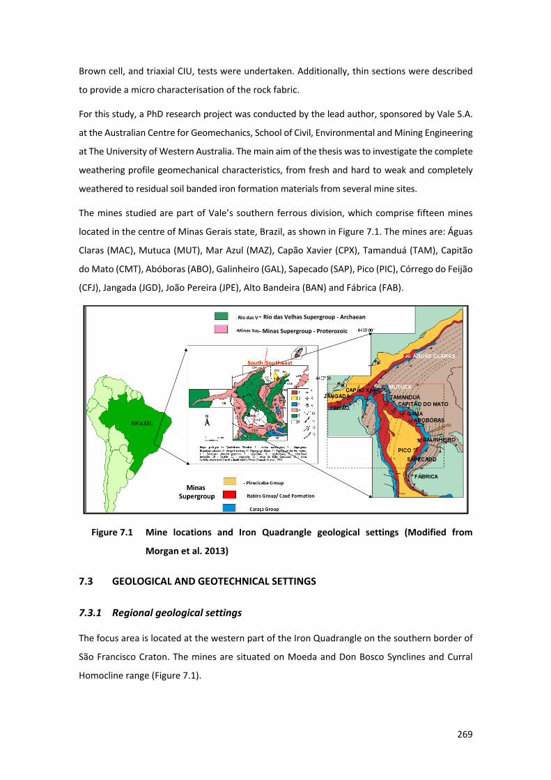
269
Brown cell, and triaxial CIU, tests were undertaken. Additionally, thin sections were described
to provide a micro characterisation of the rock fabric.
For this study, a PhD research project was conducted by the lead author, sponsored by Vale S.A.
at the Australian Centre for Geomechanics, School of Civil, Environmental and Mining Engineering
at The University of Western Australia. The main aim of the thesis was to investigate the complete
weathering profile geomechanical characteristics, from fresh and hard to weak and completely
weathered to residual soil banded iron formation materials from several mine sites.
The mines studied are part of Vale’s southern ferrous division, which comprise fifteen mines
located in the centre of Minas Gerais state, Brazil, as shown in Figure 7.1. The mines are: Águas
Claras (MAC), Mutuca (MUT), Mar Azul (MAZ), Capão Xavier (CPX), Tamanduá (TAM), Capitão
do Mato (CMT), Abóboras (ABO), Galinheiro (GAL), Sapecado (SAP), Pico (PIC), Córrego do Feijão
(CFJ), Jangada (JGD), João Pereira (JPE), Alto Bandeira (BAN) and Fábrica (FAB).
84 Figure 7.1 Mine locations and Iron Quadrangle geological settings (Modified from
Morgan et al. 2013)
7.3 GEOLOGICAL AND GEOTECHNICAL SETTINGS
7.3.1 Regional geological settings
The focus area is located at the western part of the Iron Quadrangle on the southern border of
São Francisco Craton. The mines are situated on Moeda and Don Bosco Synclines and Curral
Homocline range (Figure 7.1).
- Rio das Velhas Supergroup - Archaean - Minas Supergroup - Proterozoic
270
The structure is delineated by a roughly quadrangular arrangement, with Paleoproterozoic BIF
of the Minas Supergroup, as proposed by Dorr (1969). This supergroup is composed of hundreds
of metres of iron rich metamorphic rocks belonging to the Itabira group/Cauê Formation. The
Minas Supergroup comprises, from the bottom to the top: Caraça, Itabira, Piracicaba and Sabará
groups; a sequence of psammitic and pelitic rocks, also defined by Dorr (1969); all of which are
overlain by the Itacolomi group. Below this sequence are the Archean greenstone belt terrains
of the Rio das Velhas Supergroup and domes of Archean and Proterozoic crystalline rocks
(Machado & Carneiro 1992; Machado et al. 1989 and Noce 1995).
The Cauê Formation (Itabira Group), which hosts the BIF, is a marine chemical sequence 350 m
thick, dated 2.4 ± 0.19 Gyr by Babinski et al. (1995).
The regional structure is the result of two major deformational super-positional events, as
proposed by Chemale Jr et al. (1994). The first event produced the nucleation of regional
synclines in the uplift of the gneissic domes during the Transamazonian Orogenesis (2.1–2 Gyr);
and the second is related to an east–west verging thrust fault belt of Pan African/Brazilian age
(0.8–0.6 Gyr) described by Marshak & Alkmim (1989). This last event deformed the earlier
structures and was mainly responsible for the deformational gradient. Hertz (1978) described
an eastward increase in the metamorphic grade from green schist to lower amphibolite facies
following the deformational gradient. The structures and geological settings are also shown in
Figure 7.1.
The mines which have been studied are located in the western low strain domain and green
schist metamorphic zone, formed in the Transamazonian event. The main trend of the synclines
is north–south, but the structure has also been deformed around Bação dome. It is also
interconnected with Dom Bosco Syncline to the south and partially truncated by Engenho Fault.
To the north, it is continuous with the Serra do Curral (Curral Homocline). At the junction of
these two regional structures a northwest-verging asymmetric anticline and an interference
saddle due to the refolding were developed (Rosière et al. 1993).
The Moeda Syncline has been partially affected by the younger Brazilian tectonic event, mainly
on the eastern limb, with local development of ductile brittle to brittle shear zones. Several
strike–slip faults cut across the structure, dividing it into several segments.
The Serra do Curral hills represent the overturned south-eastern limb of a truncated northwest-
verging syncline–anticline couple, which was highly deformed and rotated by the right–lateral
movement of the northeast–southwest trending inclined ramp of a reginal thrust fault as
described by Chemale Jr et al. (1994). In this segment, the inverted northwestward limb of a
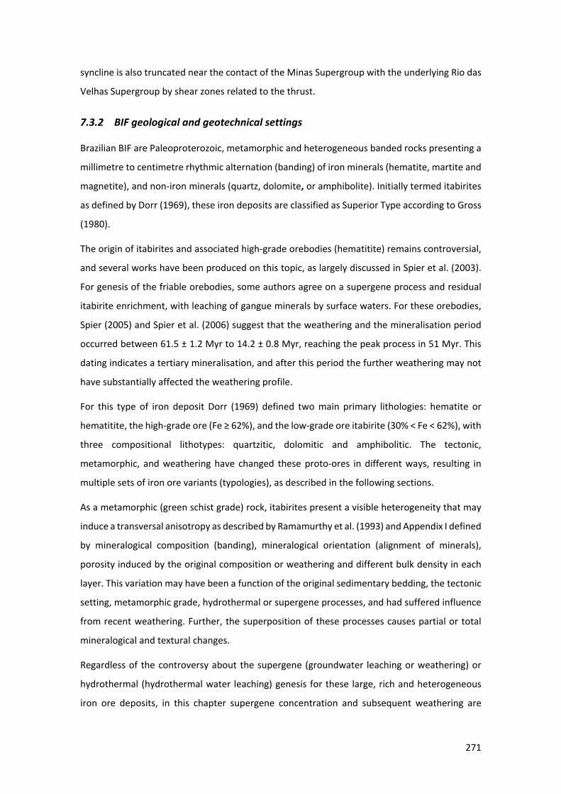
271
syncline is also truncated near the contact of the Minas Supergroup with the underlying Rio das
Velhas Supergroup by shear zones related to the thrust.
7.3.2 BIF geological and geotechnical settings
Brazilian BIF are Paleoproterozoic, metamorphic and heterogeneous banded rocks presenting a
millimetre to centimetre rhythmic alternation (banding) of iron minerals (hematite, martite and
magnetite), and non-iron minerals (quartz, dolomite, or amphibolite). Initially termed itabirites
as defined by Dorr (1969), these iron deposits are classified as Superior Type according to Gross
(1980).
The origin of itabirites and associated high-grade orebodies (hematitite) remains controversial,
and several works have been produced on this topic, as largely discussed in Spier et al. (2003).
For genesis of the friable orebodies, some authors agree on a supergene process and residual
itabirite enrichment, with leaching of gangue minerals by surface waters. For these orebodies,
Spier (2005) and Spier et al. (2006) suggest that the weathering and the mineralisation period
occurred between 61.5 ± 1.2 Myr to 14.2 ± 0.8 Myr, reaching the peak process in 51 Myr. This
dating indicates a tertiary mineralisation, and after this period the further weathering may not
have substantially affected the weathering profile.
For this type of iron deposit Dorr (1969) defined two main primary lithologies: hematite or
hematitite, the high-grade ore (Fe ≥ 62%), and the low-grade ore itabirite (30% < Fe < 62%), with
three compositional lithotypes: quartzitic, dolomitic and amphibolitic. The tectonic,
metamorphic, and weathering have changed these proto-ores in different ways, resulting in
multiple sets of iron ore variants (typologies), as described in the following sections.
As a metamorphic (green schist grade) rock, itabirites present a visible heterogeneity that may
induce a transversal anisotropy as described by Ramamurthy et al. (1993) and Appendix I defined
by mineralogical composition (banding), mineralogical orientation (alignment of minerals),
porosity induced by the original composition or weathering and different bulk density in each
layer. This variation may have been a function of the original sedimentary bedding, the tectonic
setting, metamorphic grade, hydrothermal or supergene processes, and had suffered influence
from recent weathering. Further, the superposition of these processes causes partial or total
mineralogical and textural changes.
Regardless of the controversy about the supergene (groundwater leaching or weathering) or
hydrothermal (hydrothermal water leaching) genesis for these large, rich and heterogeneous
iron ore deposits, in this chapter supergene concentration and subsequent weathering are
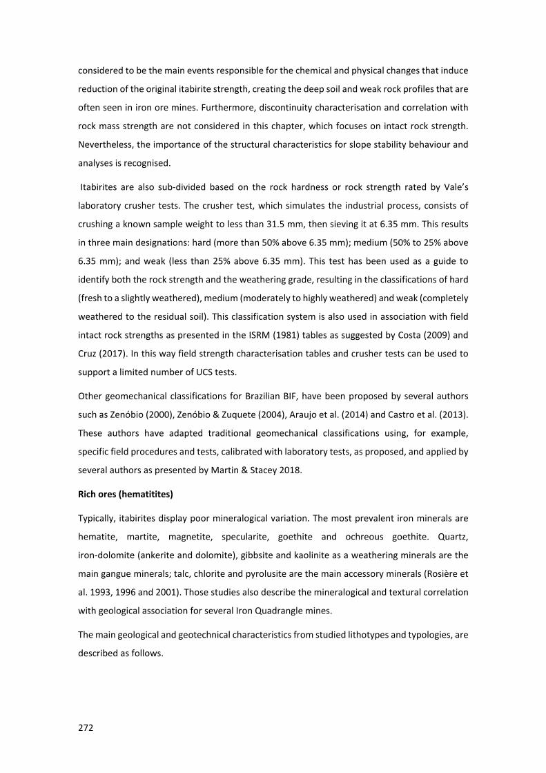
272
considered to be the main events responsible for the chemical and physical changes that induce
reduction of the original itabirite strength, creating the deep soil and weak rock profiles that are
often seen in iron ore mines. Furthermore, discontinuity characterisation and correlation with
rock mass strength are not considered in this chapter, which focuses on intact rock strength.
Nevertheless, the importance of the structural characteristics for slope stability behaviour and
analyses is recognised.
Itabirites are also sub-divided based on the rock hardness or rock strength rated by Vale’s
laboratory crusher tests. The crusher test, which simulates the industrial process, consists of
crushing a known sample weight to less than 31.5 mm, then sieving it at 6.35 mm. This results
in three main designations: hard (more than 50% above 6.35 mm); medium (50% to 25% above
6.35 mm); and weak (less than 25% above 6.35 mm). This test has been used as a guide to
identify both the rock strength and the weathering grade, resulting in the classifications of hard
(fresh to a slightly weathered), medium (moderately to highly weathered) and weak (completely
weathered to the residual soil). This classification system is also used in association with field
intact rock strengths as presented in the ISRM (1981) tables as suggested by Costa (2009) and
Cruz (2017). In this way field strength characterisation tables and crusher tests can be used to
support a limited number of UCS tests.
Other geomechanical classifications for Brazilian BIF, have been proposed by several authors
such as Zenóbio (2000), Zenóbio & Zuquete (2004), Araujo et al. (2014) and Castro et al. (2013).
These authors have adapted traditional geomechanical classifications using, for example,
specific field procedures and tests, calibrated with laboratory tests, as proposed, and applied by
several authors as presented by Martin & Stacey 2018.
Rich ores (hematitites)
Typically, itabirites display poor mineralogical variation. The most prevalent iron minerals are
hematite, martite, magnetite, specularite, goethite and ochreous goethite. Quartz,
iron-dolomite (ankerite and dolomite), gibbsite and kaolinite as a weathering minerals are the
main gangue minerals; talc, chlorite and pyrolusite are the main accessory minerals (Rosière et
al. 1993, 1996 and 2001). Those studies also describe the mineralogical and textural correlation
with geological association for several Iron Quadrangle mines.
The main geological and geotechnical characteristics from studied lithotypes and typologies, are
described as follows.
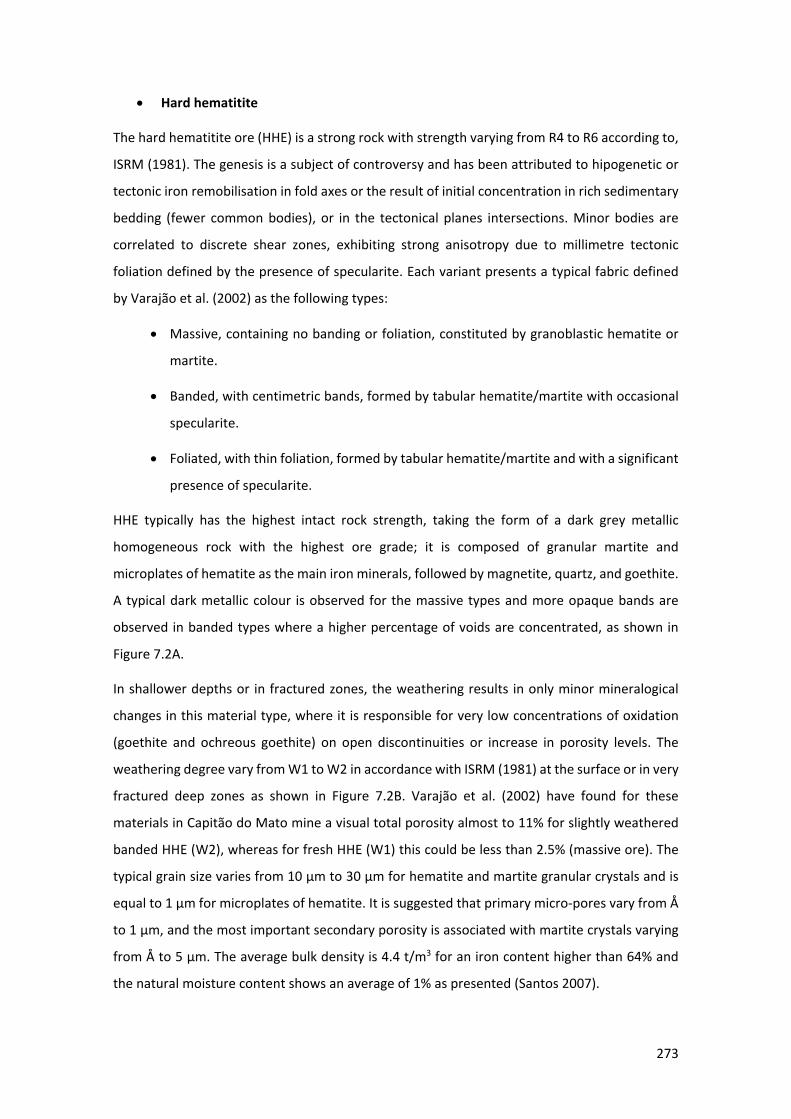
273
• Hard hematitite
The hard hematitite ore (HHE) is a strong rock with strength varying from R4 to R6 according to,
ISRM (1981). The genesis is a subject of controversy and has been attributed to hipogenetic or
tectonic iron remobilisation in fold axes or the result of initial concentration in rich sedimentary
bedding (fewer common bodies), or in the tectonical planes intersections. Minor bodies are
correlated to discrete shear zones, exhibiting strong anisotropy due to millimetre tectonic
foliation defined by the presence of specularite. Each variant presents a typical fabric defined
by Varajão et al. (2002) as the following types:
• Massive, containing no banding or foliation, constituted by granoblastic hematite or
martite.
• Banded, with centimetric bands, formed by tabular hematite/martite with occasional
specularite.
• Foliated, with thin foliation, formed by tabular hematite/martite and with a significant
presence of specularite.
HHE typically has the highest intact rock strength, taking the form of a dark grey metallic
homogeneous rock with the highest ore grade; it is composed of granular martite and
microplates of hematite as the main iron minerals, followed by magnetite, quartz, and goethite.
A typical dark metallic colour is observed for the massive types and more opaque bands are
observed in banded types where a higher percentage of voids are concentrated, as shown in
Figure 7.2A.
In shallower depths or in fractured zones, the weathering results in only minor mineralogical
changes in this material type, where it is responsible for very low concentrations of oxidation
(goethite and ochreous goethite) on open discontinuities or increase in porosity levels. The
weathering degree vary from W1 to W2 in accordance with ISRM (1981) at the surface or in very
fractured deep zones as shown in Figure 7.2B. Varajão et al. (2002) have found for these
materials in Capitão do Mato mine a visual total porosity almost to 11% for slightly weathered
banded HHE (W2), whereas for fresh HHE (W1) this could be less than 2.5% (massive ore). The
typical grain size varies from 10 μm to 30 μm for hematite and martite granular crystals and is
equal to 1 μm for microplates of hematite. It is suggested that primary micro-pores vary from Å
to 1 μm, and the most important secondary porosity is associated with martite crystals varying
from Å to 5 μm. The average bulk density is 4.4 t/m3 for an iron content higher than 64% and
the natural moisture content shows an average of 1% as presented (Santos 2007).
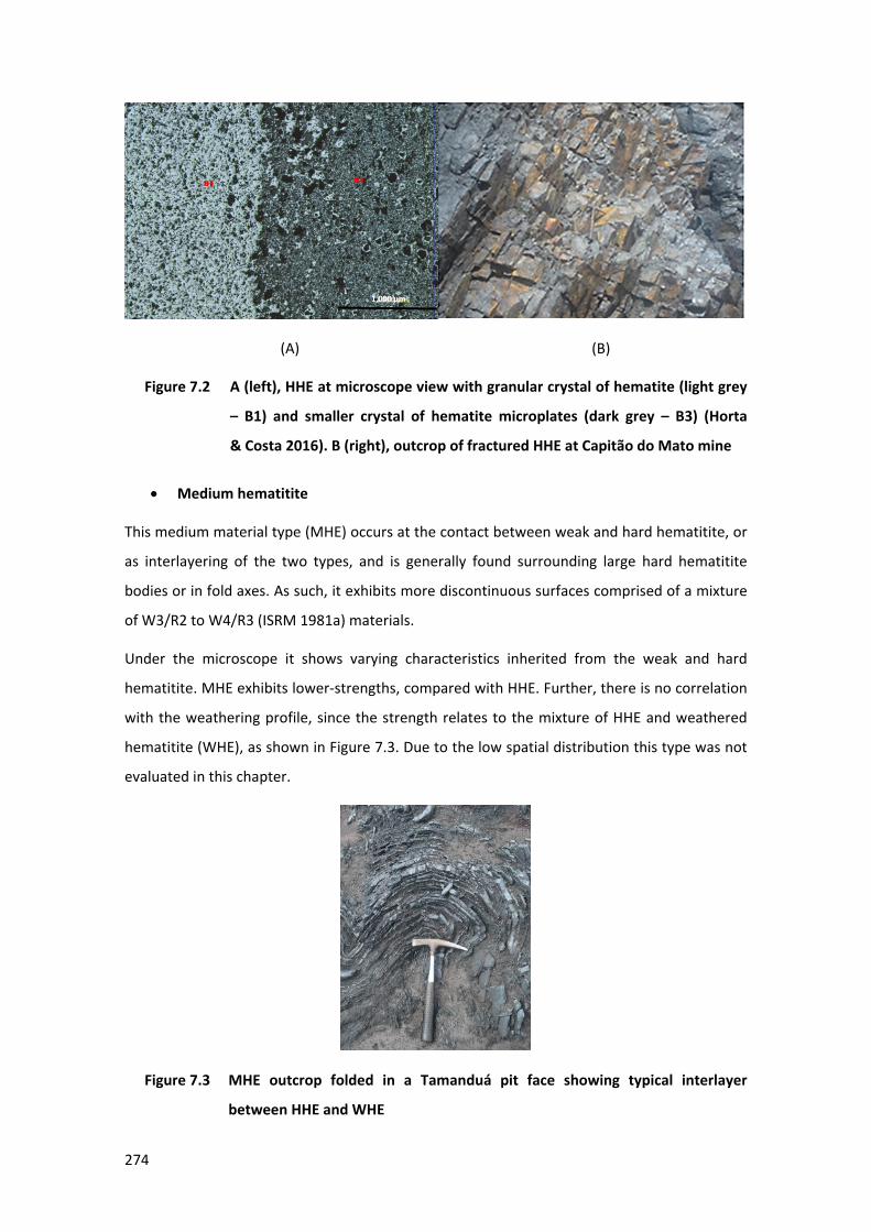
274
(A) (B)
85 Figure 7.2 A (left), HHE at microscope view with granular crystal of hematite (light grey
– B1) and smaller crystal of hematite microplates (dark grey – B3) (Horta
& Costa 2016). B (right), outcrop of fractured HHE at Capitão do Mato mine
• Medium hematitite
This medium material type (MHE) occurs at the contact between weak and hard hematitite, or
as interlayering of the two types, and is generally found surrounding large hard hematitite
bodies or in fold axes. As such, it exhibits more discontinuous surfaces comprised of a mixture
of W3/R2 to W4/R3 (ISRM 1981a) materials.
Under the microscope it shows varying characteristics inherited from the weak and hard
hematitite. MHE exhibits lower-strengths, compared with HHE. Further, there is no correlation
with the weathering profile, since the strength relates to the mixture of HHE and weathered
hematitite (WHE), as shown in Figure 7.3. Due to the low spatial distribution this type was not
evaluated in this chapter.
86 Figure 7.3 MHE outcrop folded in a Tamanduá pit face showing typical interlayer
between HHE and WHE
1,000 μm
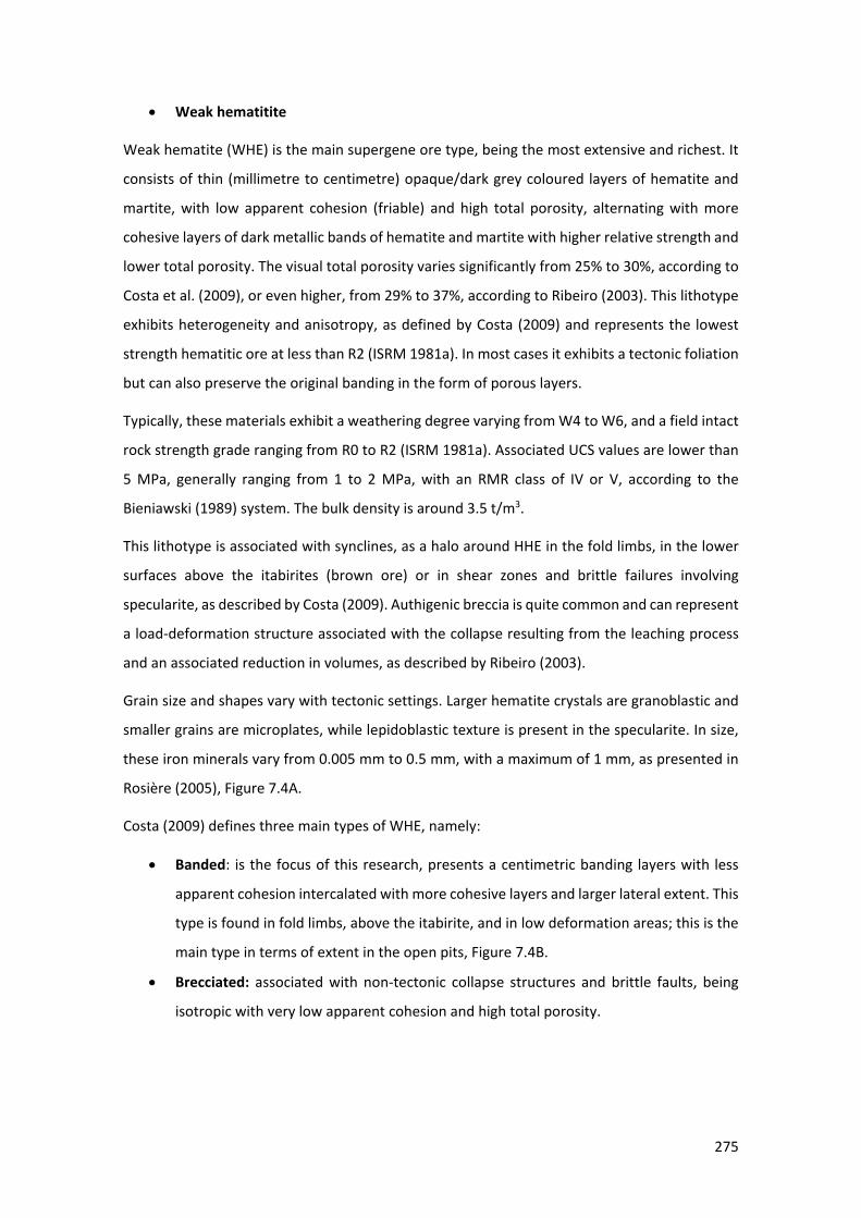
275
• Weak hematitite
Weak hematite (WHE) is the main supergene ore type, being the most extensive and richest. It
consists of thin (millimetre to centimetre) opaque/dark grey coloured layers of hematite and
martite, with low apparent cohesion (friable) and high total porosity, alternating with more
cohesive layers of dark metallic bands of hematite and martite with higher relative strength and
lower total porosity. The visual total porosity varies significantly from 25% to 30%, according to
Costa et al. (2009), or even higher, from 29% to 37%, according to Ribeiro (2003). This lithotype
exhibits heterogeneity and anisotropy, as defined by Costa (2009) and represents the lowest
strength hematitic ore at less than R2 (ISRM 1981a). In most cases it exhibits a tectonic foliation
but can also preserve the original banding in the form of porous layers.
Typically, these materials exhibit a weathering degree varying from W4 to W6, and a field intact
rock strength grade ranging from R0 to R2 (ISRM 1981a). Associated UCS values are lower than
5 MPa, generally ranging from 1 to 2 MPa, with an RMR class of IV or V, according to the
Bieniawski (1989) system. The bulk density is around 3.5 t/m3.
This lithotype is associated with synclines, as a halo around HHE in the fold limbs, in the lower
surfaces above the itabirites (brown ore) or in shear zones and brittle failures involving
specularite, as described by Costa (2009). Authigenic breccia is quite common and can represent
a load-deformation structure associated with the collapse resulting from the leaching process
and an associated reduction in volumes, as described by Ribeiro (2003).
Grain size and shapes vary with tectonic settings. Larger hematite crystals are granoblastic and
smaller grains are microplates, while lepidoblastic texture is present in the specularite. In size,
these iron minerals vary from 0.005 mm to 0.5 mm, with a maximum of 1 mm, as presented in
Rosière (2005), Figure 7.4A.
Costa (2009) defines three main types of WHE, namely:
• Banded: is the focus of this research, presents a centimetric banding layers with less
apparent cohesion intercalated with more cohesive layers and larger lateral extent. This
type is found in fold limbs, above the itabirite, and in low deformation areas; this is the
main type in terms of extent in the open pits, Figure 7.4B.
• Brecciated: associated with non-tectonic collapse structures and brittle faults, being
isotropic with very low apparent cohesion and high total porosity.
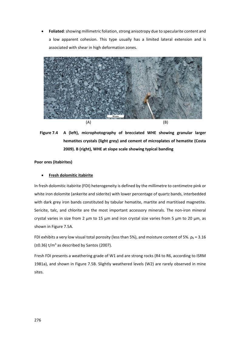
276
• Foliated: showing millimetric foliation, strong anisotropy due to specularite content and
a low apparent cohesion. This type usually has a limited lateral extension and is
associated with shear in high deformation zones.
(A) (B)
87 Figure 7.4 A (left), microphotography of brecciated WHE showing granular larger
hematites crystals (light grey) and cement of microplates of hematite (Costa
2009). B (right), WHE at slope scale showing typical banding
Poor ores (itabirites)
• Fresh dolomitic itabirite
In fresh dolomitic itabirite (FDI) heterogeneity is defined by the millimetre to centimetre pink or
white iron dolomite (ankerite and siderite) with lower percentage of quartz bands, interbedded
with dark grey iron bands constituted by tabular hematite, martite and martitised magnetite.
Sericite, talc, and chlorite are the most important accessory minerals. The non-iron mineral
crystal varies in size from 2 µm to 15 µm and iron crystal size varies from 5 µm to 20 µm, as
shown in Figure 7.5A.
FDI exhibits a very low visual total porosity (less than 5%), and moisture content of 5%. ρb = 3.16
(±0.36) t/m3 as described by Santos (2007).
Fresh FDI presents a weathering grade of W1 and are strong rocks (R4 to R6, according to ISRM
1981a), and shown in Figure 7.5B. Slightly weathered levels (W2) are rarely observed in mine
sites.
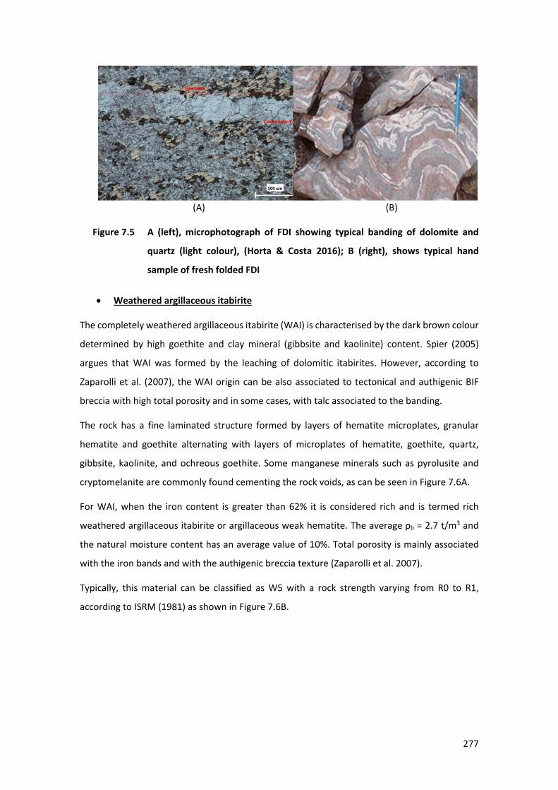
277
(A) (B)
88 Figure 7.5 A (left), microphotograph of FDI showing typical banding of dolomite and
quartz (light colour), (Horta & Costa 2016); B (right), shows typical hand
sample of fresh folded FDI
• Weathered argillaceous itabirite
The completely weathered argillaceous itabirite (WAI) is characterised by the dark brown colour
determined by high goethite and clay mineral (gibbsite and kaolinite) content. Spier (2005)
argues that WAI was formed by the leaching of dolomitic itabirites. However, according to
Zaparolli et al. (2007), the WAI origin can be also associated to tectonical and authigenic BIF
breccia with high total porosity and in some cases, with talc associated to the banding.
The rock has a fine laminated structure formed by layers of hematite microplates, granular
hematite and goethite alternating with layers of microplates of hematite, goethite, quartz,
gibbsite, kaolinite, and ochreous goethite. Some manganese minerals such as pyrolusite and
cryptomelanite are commonly found cementing the rock voids, as can be seen in Figure 7.6A.
For WAI, when the iron content is greater than 62% it is considered rich and is termed rich
weathered argillaceous itabirite or argillaceous weak hematite. The average ρb = 2.7 t/m3 and
the natural moisture content has an average value of 10%. Total porosity is mainly associated
with the iron bands and with the authigenic breccia texture (Zaparolli et al. 2007).
Typically, this material can be classified as W5 with a rock strength varying from R0 to R1,
according to ISRM (1981) as shown in Figure 7.6B.
500 μm
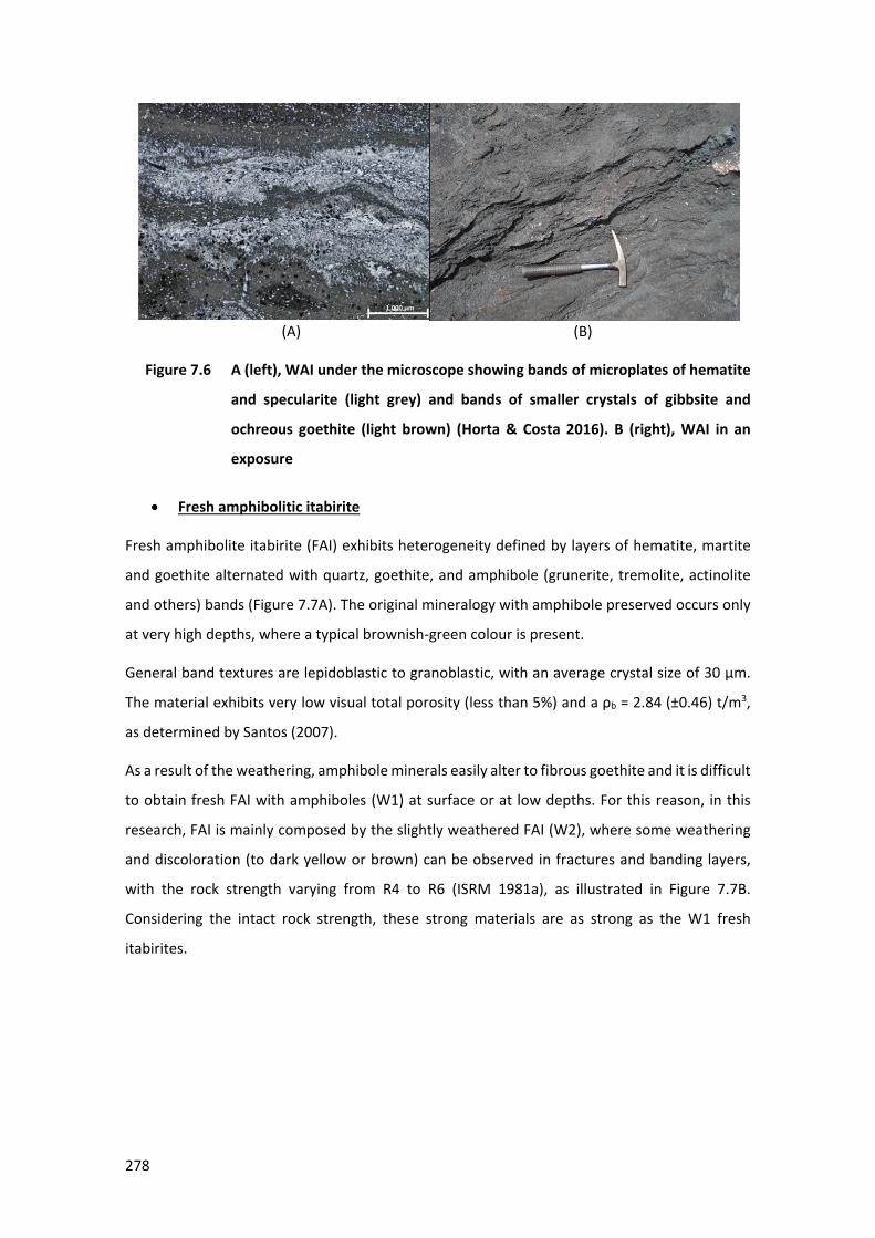
278
(A) (B)
89 Figure 7.6 A (left), WAI under the microscope showing bands of microplates of hematite
and specularite (light grey) and bands of smaller crystals of gibbsite and
ochreous goethite (light brown) (Horta & Costa 2016). B (right), WAI in an
exposure
• Fresh amphibolitic itabirite
Fresh amphibolite itabirite (FAI) exhibits heterogeneity defined by layers of hematite, martite
and goethite alternated with quartz, goethite, and amphibole (grunerite, tremolite, actinolite
and others) bands (Figure 7.7A). The original mineralogy with amphibole preserved occurs only
at very high depths, where a typical brownish-green colour is present.
General band textures are lepidoblastic to granoblastic, with an average crystal size of 30 µm.
The material exhibits very low visual total porosity (less than 5%) and a ρb = 2.84 (±0.46) t/m3,
as determined by Santos (2007).
As a result of the weathering, amphibole minerals easily alter to fibrous goethite and it is difficult
to obtain fresh FAI with amphiboles (W1) at surface or at low depths. For this reason, in this
research, FAI is mainly composed by the slightly weathered FAI (W2), where some weathering
and discoloration (to dark yellow or brown) can be observed in fractures and banding layers,
with the rock strength varying from R4 to R6 (ISRM 1981a), as illustrated in Figure 7.7B.
Considering the intact rock strength, these strong materials are as strong as the W1 fresh
itabirites.
1,000 μm
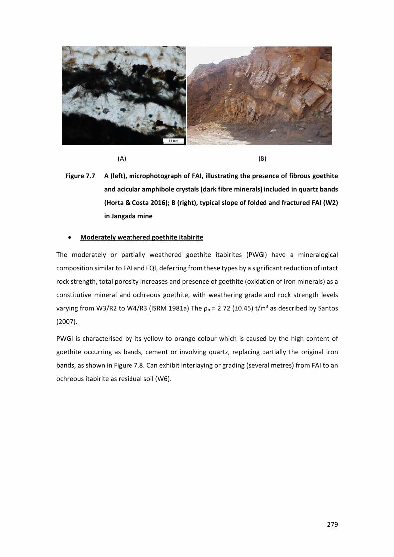
279
(A) (B)
90 Figure 7.7 A (left), microphotograph of FAI, illustrating the presence of fibrous goethite
and acicular amphibole crystals (dark fibre minerals) included in quartz bands
(Horta & Costa 2016); B (right), typical slope of folded and fractured FAI (W2)
in Jangada mine
• Moderately weathered goethite itabirite
The moderately or partially weathered goethite itabirites (PWGI) have a mineralogical
composition similar to FAI and FQI, deferring from these types by a significant reduction of intact
rock strength, total porosity increases and presence of goethite (oxidation of iron minerals) as a
constitutive mineral and ochreous goethite, with weathering grade and rock strength levels
varying from W3/R2 to W4/R3 (ISRM 1981a) The ρb = 2.72 (±0.45) t/m3 as described by Santos
(2007).
PWGI is characterised by its yellow to orange colour which is caused by the high content of
goethite occurring as bands, cement or involving quartz, replacing partially the original iron
bands, as shown in Figure 7.8. Can exhibit interlaying or grading (several metres) from FAI to an
ochreous itabirite as residual soil (W6).
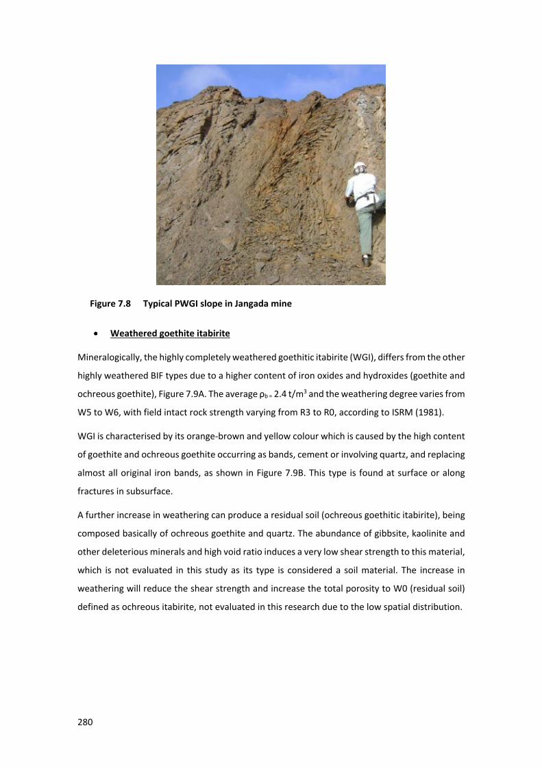
280
91 Figure 7.8 Typical PWGI slope in Jangada mine
• Weathered goethite itabirite
Mineralogically, the highly completely weathered goethitic itabirite (WGI), differs from the other
highly weathered BIF types due to a higher content of iron oxides and hydroxides (goethite and
ochreous goethite), Figure 7.9A. The average ρb = 2.4 t/m3 and the weathering degree varies from
W5 to W6, with field intact rock strength varying from R3 to R0, according to ISRM (1981).
WGI is characterised by its orange-brown and yellow colour which is caused by the high content
of goethite and ochreous goethite occurring as bands, cement or involving quartz, and replacing
almost all original iron bands, as shown in Figure 7.9B. This type is found at surface or along
fractures in subsurface.
A further increase in weathering can produce a residual soil (ochreous goethitic itabirite), being
composed basically of ochreous goethite and quartz. The abundance of gibbsite, kaolinite and
other deleterious minerals and high void ratio induces a very low shear strength to this material,
which is not evaluated in this study as its type is considered a soil material. The increase in
weathering will reduce the shear strength and increase the total porosity to W0 (residual soil)
defined as ochreous itabirite, not evaluated in this research due to the low spatial distribution.
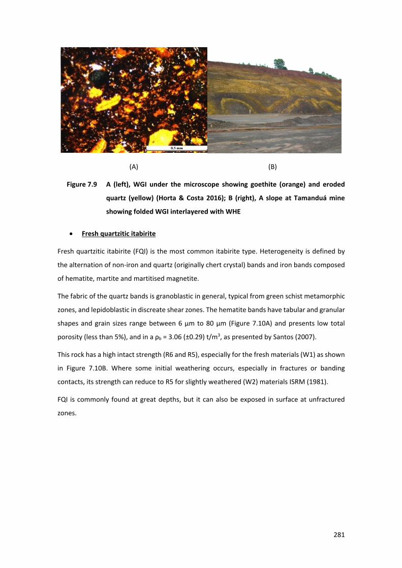
281
(A) (B)
92 Figure 7.9 A (left), WGI under the microscope showing goethite (orange) and eroded
quartz (yellow) (Horta & Costa 2016); B (right), A slope at Tamanduá mine
showing folded WGI interlayered with WHE
• Fresh quartzitic itabirite
Fresh quartzitic itabirite (FQI) is the most common itabirite type. Heterogeneity is defined by
the alternation of non-iron and quartz (originally chert crystal) bands and iron bands composed
of hematite, martite and martitised magnetite.
The fabric of the quartz bands is granoblastic in general, typical from green schist metamorphic
zones, and lepidoblastic in discreate shear zones. The hematite bands have tabular and granular
shapes and grain sizes range between 6 µm to 80 µm (Figure 7.10A) and presents low total
porosity (less than 5%), and in a ρb = 3.06 (±0.29) t/m3, as presented by Santos (2007).
This rock has a high intact strength (R6 and R5), especially for the fresh materials (W1) as shown
in Figure 7.10B. Where some initial weathering occurs, especially in fractures or banding
contacts, its strength can reduce to R5 for slightly weathered (W2) materials ISRM (1981).
FQI is commonly found at great depths, but it can also be exposed in surface at unfractured
zones.
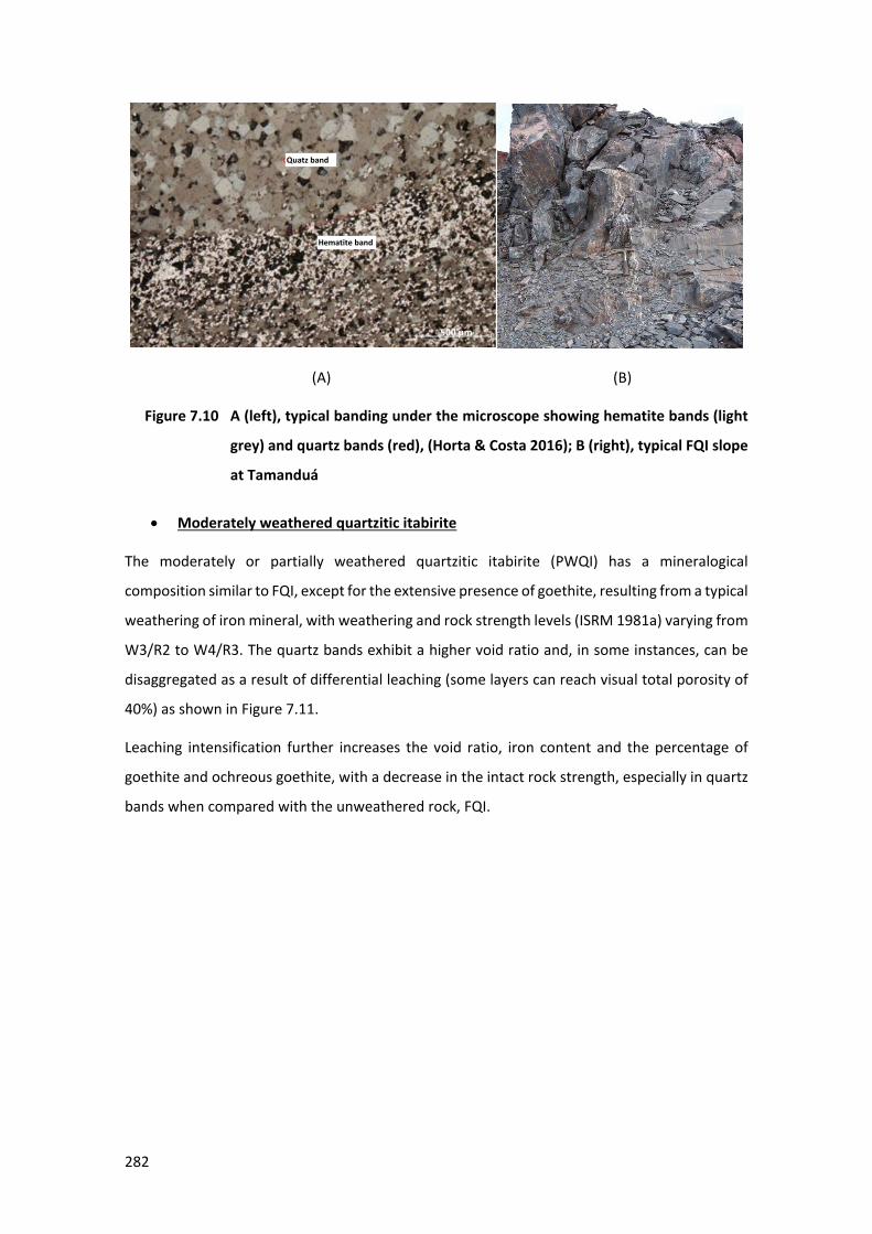
282
(A) (B)
93 Figure 7.10 A (left), typical banding under the microscope showing hematite bands (light
grey) and quartz bands (red), (Horta & Costa 2016); B (right), typical FQI slope
at Tamanduá
• Moderately weathered quartzitic itabirite
The moderately or partially weathered quartzitic itabirite (PWQI) has a mineralogical
composition similar to FQI, except for the extensive presence of goethite, resulting from a typical
weathering of iron mineral, with weathering and rock strength levels (ISRM 1981a) varying from
W3/R2 to W4/R3. The quartz bands exhibit a higher void ratio and, in some instances, can be
disaggregated as a result of differential leaching (some layers can reach visual total porosity of
40%) as shown in Figure 7.11.
Leaching intensification further increases the void ratio, iron content and the percentage of
goethite and ochreous goethite, with a decrease in the intact rock strength, especially in quartz
bands when compared with the unweathered rock, FQI.
500 μm
Quatz band
Hematite band
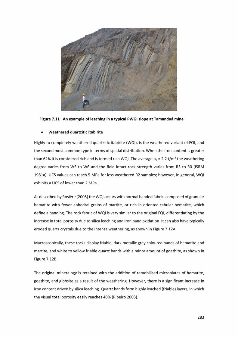
283
94 Figure 7.11 An example of leaching in a typical PWGI slope at Tamanduá mine
• Weathered quartzitic itabirite
Highly to completely weathered quartzitic itabirite (WQI), is the weathered variant of FQI, and
the second most common type in terms of spatial distribution. When the iron content is greater
than 62% it is considered rich and is termed rich WQI. The average ρb = 2.2 t/m3 the weathering
degree varies from W5 to W6 and the field intact rock strength varies from R3 to R0 (ISRM
1981a). UCS values can reach 5 MPa for less weathered R2 samples; however, in general, WQI
exhibits a UCS of lower than 2 MPa.
As described by Rosière (2005) the WQI occurs with normal banded fabric, composed of granular
hematite with fewer anhedral grains of martite, or rich in oriented tabular hematite, which
define a banding. The rock fabric of WQI is very similar to the original FQI, differentiating by the
increase in total porosity due to silica leaching and iron band oxidation. It can also have typically
eroded quartz crystals due to the intense weathering, as shown in Figure 7.12A.
Macroscopically, these rocks display friable, dark metallic grey coloured bands of hematite and
martite, and white to yellow friable quartz bands with a minor amount of goethite, as shown in
Figure 7.12B.
The original mineralogy is retained with the addition of remobilised microplates of hematite,
goethite, and gibbsite as a result of the weathering. However, there is a significant increase in
iron content driven by silica leaching. Quartz bands form highly leached (friable) layers, in which
the visual total porosity easily reaches 40% (Ribeiro 2003).
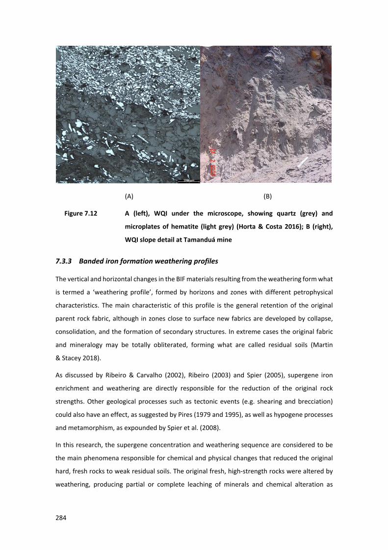
284
(A) (B)
95 Figure 7.12 A (left), WQI under the microscope, showing quartz (grey) and
microplates of hematite (light grey) (Horta & Costa 2016); B (right),
WQI slope detail at Tamanduá mine
7.3.3 Banded iron formation weathering profiles
The vertical and horizontal changes in the BIF materials resulting from the weathering form what
is termed a ‘weathering profile’, formed by horizons and zones with different petrophysical
characteristics. The main characteristic of this profile is the general retention of the original
parent rock fabric, although in zones close to surface new fabrics are developed by collapse,
consolidation, and the formation of secondary structures. In extreme cases the original fabric
and mineralogy may be totally obliterated, forming what are called residual soils (Martin
& Stacey 2018).
As discussed by Ribeiro & Carvalho (2002), Ribeiro (2003) and Spier (2005), supergene iron
enrichment and weathering are directly responsible for the reduction of the original rock
strengths. Other geological processes such as tectonic events (e.g. shearing and brecciation)
could also have an effect, as suggested by Pires (1979 and 1995), as well as hypogene processes
and metamorphism, as expounded by Spier et al. (2008).
In this research, the supergene concentration and weathering sequence are considered to be
the main phenomena responsible for chemical and physical changes that reduced the original
hard, fresh rocks to weak residual soils. The original fresh, high-strength rocks were altered by
weathering, producing partial or complete leaching of minerals and chemical alteration as
1000 μm
285
postulated by Dorr (1969), Varajão et al. (1997); Ribeiro (2003); Spier et al. (2006); Ramanaidou
(2009); Ramanaidou & Morris (2010).
In the field of geotechnical engineering, there is a great diversity of terminology used to describe
and classify the various components of a weathering profile, and the terms residual soil and
saprolite are often misused. Many authors have proposed their own terminology to designate
the different layers of a weathering profile. In this research, the weathering profile proposed by
Deere & Patton (1971) is used.
As proposed by Dorr (1969), the effectiveness of the weathering in the Iron Quadrangle (IQ) was
induced by a high temperature range, high pluviometry (rainfall), favourable topography, the
high primary and secondary permeability of BIF rocks structural control as synclines and
anticlines, banding with steep dip angles and extensional fractures. All of these factors facilitate
superficial and groundwater circulation, thereby enhancing chemical and physical weathering
and, thus developing deep weathering profiles that can often reach to over 400 m in depth.
Evaluating the ‘canga’ material origin, Spier et al. (2019), propose a genetic and evolution model
of the weathering profile for itabirites within the IQ, comprising a sequence of chemical
weathering and pedogenic processes. This model allows an independence of the pedolith
(ferruginous duricrust of canga) and saprolite (supergene iron ore) formation processes and the
evolution of weathering profiles developed in itabirite. It also indicates that weathering is less
effective in quartzitic itabirite than in dolomitic itabirite, resulting in different sized ore bodies
and geochemical trends.
As outlined, by Ramanaidou & Morris (2010), supergene iron enrichment and subsequent
strength reduction can be divided into two main processes:
• The supergene mimetic mechanism occurs below the watertable, as described by
Morris (1980) and Morris (2002, 2002a and 2003) and is associated with the presence
of structures, topography and climate. It is also responsible for producing deep and large
iron-rich deposits.
• The supergene lateritic mechanism is the result of gangue minerals dissolution and iron
reconcentration above the watertable. This process produces several weathering
profiles characterised by different relative iron enrichment and gangue mineral
composition.
Mineral changes are not the only noted effect of the chemical weathering process. Total porosity
increases are also recognised as an important change observed in those rocks. Studies by Morris
(2002 and 2002a) and Taylor et al. (2001) argue that the supergene process can reduce the
286
thickness of BIFs by 32% to 40% and increase total porosity from 6% to 30% (Mourão 2007). This
information is in accordance with conclusions by Aylmer et al. (1978) when evaluating bulk
density, iron grade and total porosity for Mount Tom Price iron mine. These authors concluded
that iron grade and bulk density have a good correlation. However, this correlation accuracy is
affected by high values and variability of the total porosity.
According to Box & Reid (1976), for iron ore formation from Cockatoo Island, the true specific
gravity could be expressed as a function of iron content. However, due to the complexity and
the influence of multiple factors, the same could not be established for total porosity. Thomson
(1963) concludes that, for iron ore samples from Australia, a theoretical hematite quartz curve
can be used for bulk density definition and can allow an approximate iron content calculation.
The same relationship was identified for South African iron ore by Nel (2007); this study
established that for Sishen deposits total porosity is directly correlated to dry and bulk density,
providing a reliable calculation index.
For Vale’s iron ore mines in Brazil, studies by; Santos (2007), Santos et al. (2005) and Ribeiro et
al. (2014), have evaluated the association between bulk density and iron content for the IQ BIF
and concluded that there is a positive linear correlation between total iron content and bulk
density. Also, these authors argue that the weathering has an important influence on bulk
density and iron content variability as a function of the effective porosity.
7.3.4 Failure criteria evaluation for the BIF’s weathering profiles
In the IQ iron ore mines, due to the predominance of weak rocks and soil material, the
Mohr–Coulomb failure criterion (MC) has often been used to define the strength parameters
required for slope stability analyses, based on direct shear and triaxial shear tests. For soil
materials the Mohr–Coulomb criterion is the simplest and most widely used constitutive model
for determining the normal and shear stresses at failure on a loaded frictional material. Bai et
al. (2010) argue that MC has been widely used in rock and soil mechanics and has good
resolution for materials that fail in the elastic range and under low strain plasticity.
However, with increasing quantities of hard rocks in deeper mines it has become necessary to
perform specific tests for these materials and, due to the popularity of the Hoek–Brown failure
criterion (HB), the unconfined compression test (UCS) has become the most important rock
strength test applicable for hard rocks. In the absence of a suitable number of these tests,
geomechanical field classification and empirical correlations with petrophysical characteristics
were used to provide input for slope stability analyses.
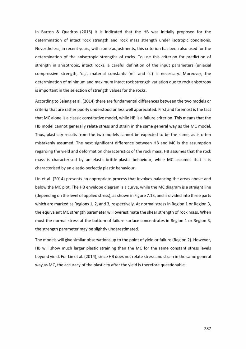
287
In Barton & Quadros (2015) it is indicated that the HB was initially proposed for the
determination of intact rock strength and rock mass strength under isotropic conditions.
Nevertheless, in recent years, with some adjustments, this criterion has been also used for the
determination of the anisotropic strengths of rocks. To use this criterion for prediction of
strength in anisotropic, intact rocks, a careful definition of the input parameters (uniaxial
compressive strength, ‘σci’, material constants ‘mi’ and ‘s’) is necessary. Moreover, the
determination of minimum and maximum intact rock strength variation due to rock anisotropy
is important in the selection of strength values for the rocks.
According to Saiang et al. (2014) there are fundamental differences between the two models or
criteria that are rather poorly understood or less well appreciated. First and foremost is the fact
that MC alone is a classic constitutive model, while HB is a failure criterion. This means that the
HB model cannot generally relate stress and strain in the same general way as the MC model.
Thus, plasticity results from the two models cannot be expected to be the same, as is often
mistakenly assumed. The next significant difference between HB and MC is the assumption
regarding the yield and deformation characteristics of the rock mass. HB assumes that the rock
mass is characterised by an elastic-brittle-plastic behaviour, while MC assumes that it is
characterised by an elastic-perfectly plastic behaviour.
Lin et al. (2014) presents an appropriate process that involves balancing the areas above and
below the MC plot. The HB envelope diagram is a curve, while the MC diagram is a straight line
(depending on the level of applied stress), as shown in Figure 7.13, and is divided into three parts
which are marked as Regions 1, 2, and 3, respectively. At normal stress in Region 1 or Region 3,
the equivalent MC strength parameter will overestimate the shear strength of rock mass. When
most the normal stress at the bottom of failure surface concentrates in Region 1 or Region 3,
the strength parameter may be slightly underestimated.
The models will give similar observations up to the point of yield or failure (Region 2). However,
HB will show much larger plastic straining than the MC for the same constant stress levels
beyond yield. For Lin et al. (2014), since HB does not relate stress and strain in the same general
way as MC, the accuracy of the plasticity after the yield is therefore questionable.
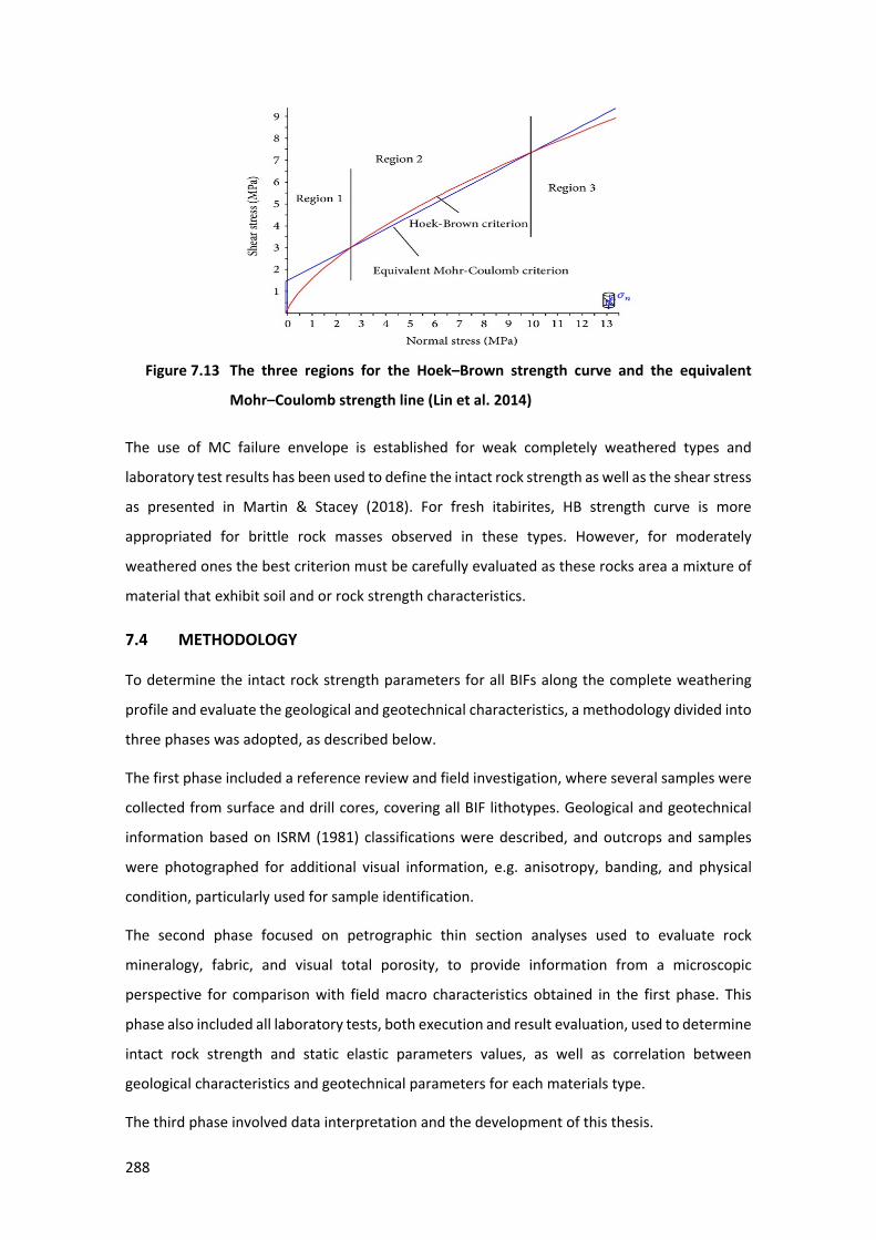
288
96 Figure 7.13 The three regions for the Hoek–Brown strength curve and the equivalent
Mohr–Coulomb strength line (Lin et al. 2014)
The use of MC failure envelope is established for weak completely weathered types and
laboratory test results has been used to define the intact rock strength as well as the shear stress
as presented in Martin & Stacey (2018). For fresh itabirites, HB strength curve is more
appropriated for brittle rock masses observed in these types. However, for moderately
weathered ones the best criterion must be carefully evaluated as these rocks area a mixture of
material that exhibit soil and or rock strength characteristics.
7.4 METHODOLOGY
To determine the intact rock strength parameters for all BIFs along the complete weathering
profile and evaluate the geological and geotechnical characteristics, a methodology divided into
three phases was adopted, as described below.
The first phase included a reference review and field investigation, where several samples were
collected from surface and drill cores, covering all BIF lithotypes. Geological and geotechnical
information based on ISRM (1981) classifications were described, and outcrops and samples
were photographed for additional visual information, e.g. anisotropy, banding, and physical
condition, particularly used for sample identification.
The second phase focused on petrographic thin section analyses used to evaluate rock
mineralogy, fabric, and visual total porosity, to provide information from a microscopic
perspective for comparison with field macro characteristics obtained in the first phase. This
phase also included all laboratory tests, both execution and result evaluation, used to determine
intact rock strength and static elastic parameters values, as well as correlation between
geological characteristics and geotechnical parameters for each materials type.
The third phase involved data interpretation and the development of this thesis.
289
Brazilian and Australian laboratories were used to carried out geotechnical tests and provide
proper results used to support the aims of this research. Data from previous laboratory test
reports (available in Vale’s database) and laboratory test results from other authors were
occasionally used to address the lack of information identified for some types.
The first step in the laboratory test program was to define the appropriate geotechnical tests
for each weathering grade. Due to the high-strength variations noted in the weathering profile
and the difficulty in preparing samples with high-strength heterogeneity, mainly for partially
weathered types, the rock strength estimation table from Martin & Stacey (2018) was used to
define a hypothetical strength limit for the three groups of BIF (fresh, moderately an completely
weathered) and associated laboratory tests, as shown in Figure 7.14.
For hard rocks with high-strength and fresh to slightly weathering grade associated to bedrock
horizon (green dotted line) the unconfined compressive strength (UCS), triaxial Hoek cell
(TRI-HB) and indirect unconfined tensile strength (UTS) were used. For weak rocks with low to
very low strengths and highly to completely weathered associated with saprolite and residual
soil weathering grades (red dotted line), single stage consolidated undrained triaxial
compression test (CIU) was applied. For moderate strength and weathering grade values
associated with saprorock (blue dotted lines), where materials exhibit variable strength
behaviour, tests were selected in accordance with the predominant strength characteristic in
each sample (soil for saprolite or saprorock for rock). For all samples, physical tests were carried
out to determine the bulk density and visual total porosity.
97 Figure 7.14 Weathering grade and estimation of the rock strength table plotted for the three
main weathered groups. The applied laboratory tests for each strength level are
grouped by the green dotted square for hard rocks (bedrock), a blue dotted
square for moderate rock (saprorock) strength and the red dotted square for
weak rock (saprolite) and soil-like material strength (after Martin & Stacey 2018)
290
Often large variations in values of the strength of rock samples are attributed to accuracy of
sample preparation or testing procedures. However, high variance also results from intrinsic
characteristics of sample negligence during sample selection and grouping. In order to reduce
variability due to geological effects and defects, the sampling validation approach presented in
Appendix I, which suggests a sample grouping to reduce the variance and provides better
lithotype characterisation, was used. This approach was proposed to check the samples before
carrying out the tests, and considers:
• Samples were grouped by the level of weathering based on ISRM (1981), geological
characteristics (e.g. banding features), transverse isotropy direction (βangle) and ρb.
• For fresh rocks, Vp measurements were used to discard inadequate samples (inclusions
or fractured).
• Geological features such as intense folding, the presence of significant specularite and
chlorite, fracture filling materials with a different degree of weathering, quartz or calcite
veins and others that do not represent the typical BIF heterogeneity were discarded.
• Itabirites samples that did not show typical banding were not evaluated, thereby
heterogeneity defined by the compositional metamorphic banding was included and
qualitatively evaluated. The bands thickness was qualitatively considered to the
sample size in order to avoid the scale effect.
• Extreme outlier results were removed according to the box plot statistical
methodology (Whitaker et al. 2013). This technique identifies the mild outlier’s values
from the quartiles (Qt) determination, based on the Equation 7.1.
Values below the lower inner fence (QtLower):
QtLower = 1Qt - 1.5(3Qt - 1Qt) (7.1)
and values above the upper inner fence (Qtupper) as Equation 7.2:
Qtupper = 3Qt + 1.5(3Qt - 1Qt) (7.2)
where 1Qt is the first quartile and 3Qt is the third quartile.
The 3Qt evaluates database dispersion around a central data leaving 75% of data
below the sum and is defined by Equation 7.3:
3Qt = × + 1.5.IQR (7.3)
The 1Qt evaluates database dispersion around a central data leaving 25% of data
below the sum and is defined by the Equation 7.4.
291
1Qt = × - 1.5.IQR (7.4)
Interquartile ranges (IQR) measure how spread out from a central data the values are
and these form what are called outliers and are defined by Equation 7.5:
IQR = 3Qt - 1Qt (7.5)
To provide a basis for anisotropy evaluation, different mathematical approaches were used to
make comparisons between different lithotypes and parameters, depending on the number of
test results. When the number of test results was lower than 10 (n < 10) the arithmetic mean
(mean), obtained by summing the data results and then dividing by the number of samples or
variables, was used. When the number of test results was higher than 10 (n ≥ 10) basic statistical
evaluations (arithmetic mean, standard deviation, coefficient of variance, and maximum and
minimum values) were applied. These values were used with a confidence interval of 95%.
The basic statistical analyses allow a clear pattern of values results and variation and thus the
decision making of the most assertive parameters possible to be used.
The anisotropy of a rock is the property which allows it to present, for the same physical
property, different results in different directions and the degree or ratio of anisotropy is used to
quantify how far the rock is from being isotropic. For geotechnical rock characterisation, the
main physical property used to determine the anisotropy is the rock strength. The term
heterogeneity is used for rocks composed by layers or bands (scale related) that are different
from one another that could, or could not present, for the same physical properties, different
results in different directions.
For BIF which presents metamorphic heterogeneous banding, it is necessary to determine the
ratio of anisotropy to evaluate the anisotropy behaviour. Estimating the variation of intact rock
strength due to anisotropy effect allows the differentiation of spurious test results induced by
rock intrinsic characteristics which can lead to misleading results and increasing variance. In the
present study, the variation of UCS due to anisotropy was considered and was determined by
the degree of strength anisotropy (RC), as firstly proposed by Singh et al. (1989) with defines the
degree of anisotropy as the variation in compressive strength (measured in uniaxial and triaxial
tests) depending on the angle between the direction of the load applied to the tested samples
and the direction of the anisotropy.
In order to evaluate the influence of metamorphic banding and define an anisotropy in intact
rock strength for all tests, the anisotropy (βangle) as described by Jaeger (1960) was considered,
by testing different angles between banding and the loading direction, varying from 0° to 90°.
However, due to the reduced number of valid results for some typologies, results were grouped
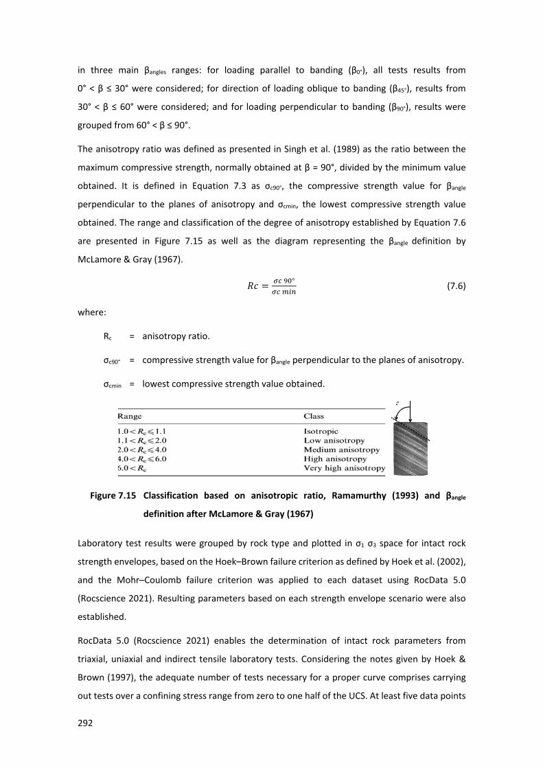
292
in three main βangles ranges: for loading parallel to banding (β0°), all tests results from
0° < β ≤ 30° were considered; for direction of loading oblique to banding (β45°), results from
30° < β ≤ 60° were considered; and for loading perpendicular to banding (β90°), results were
grouped from 60° < β ≤ 90°.
The anisotropy ratio was defined as presented in Singh et al. (1989) as the ratio between the
maximum compressive strength, normally obtained at β = 90°, divided by the minimum value
obtained. It is defined in Equation 7.3 as σc90°, the compressive strength value for βangle
perpendicular to the planes of anisotropy and σcmin, the lowest compressive strength value
obtained. The range and classification of the degree of anisotropy established by Equation 7.6
are presented in Figure 7.15 as well as the diagram representing the βangle definition by
McLamore & Gray (1967).
𝑅𝑅𝑅𝑅 = 𝜎𝜎𝜎𝜎 90°𝜎𝜎𝜎𝜎 𝑚𝑚𝑚𝑚𝑚𝑚
(7.6)
where:
Rc = anisotropy ratio.
σc90° = compressive strength value for βangle perpendicular to the planes of anisotropy.
σcmin = lowest compressive strength value obtained.
98 Figure 7.15 Classification based on anisotropic ratio, Ramamurthy (1993) and βangle
definition after McLamore & Gray (1967)
Laboratory test results were grouped by rock type and plotted in σ1 σ3 space for intact rock
strength envelopes, based on the Hoek–Brown failure criterion as defined by Hoek et al. (2002),
and the Mohr–Coulomb failure criterion was applied to each dataset using RocData 5.0
(Rocscience 2021). Resulting parameters based on each strength envelope scenario were also
established.
RocData 5.0 (Rocscience 2021) enables the determination of intact rock parameters from
triaxial, uniaxial and indirect tensile laboratory tests. Considering the notes given by Hoek &
Brown (1997), the adequate number of tests necessary for a proper curve comprises carrying
out tests over a confining stress range from zero to one half of the UCS. At least five data points
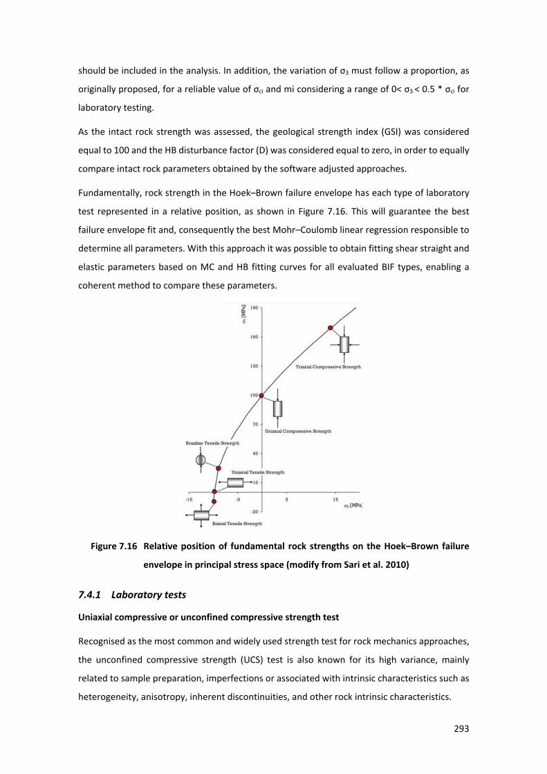
293
should be included in the analysis. In addition, the variation of σ3 must follow a proportion, as
originally proposed, for a reliable value of σci and mi considering a range of 0< σ3 < 0.5 * σci for
laboratory testing.
As the intact rock strength was assessed, the geological strength index (GSI) was considered
equal to 100 and the HB disturbance factor (D) was considered equal to zero, in order to equally
compare intact rock parameters obtained by the software adjusted approaches.
Fundamentally, rock strength in the Hoek–Brown failure envelope has each type of laboratory
test represented in a relative position, as shown in Figure 7.16. This will guarantee the best
failure envelope fit and, consequently the best Mohr–Coulomb linear regression responsible to
determine all parameters. With this approach it was possible to obtain fitting shear straight and
elastic parameters based on MC and HB fitting curves for all evaluated BIF types, enabling a
coherent method to compare these parameters.
99 Figure 7.16 Relative position of fundamental rock strengths on the Hoek–Brown failure
envelope in principal stress space (modify from Sari et al. 2010)
7.4.1 Laboratory tests
Uniaxial compressive or unconfined compressive strength test
Recognised as the most common and widely used strength test for rock mechanics approaches,
the unconfined compressive strength (UCS) test is also known for its high variance, mainly
related to sample preparation, imperfections or associated with intrinsic characteristics such as
heterogeneity, anisotropy, inherent discontinuities, and other rock intrinsic characteristics.
294
Selected rock samples from drill cores were sub-sampled, reviewed and prepared according to
ASTM D4543-01 (ASTM 2001). Final preparation of the samples involved the formation of
perfectly parallel ends to obtain perfect coupling.
The first set of UCS tests was carried out at an Australian laboratory following ASTM D2938-95
(ASTM 2002). Samples (cylindrical) were obtained from the original 77.8 mm cores using a
diamond drill bit, which sub-sampled to a 20 mm diameter, with lengths ranging from 40 mm to
50 mm, according to ASTM D4543-01 (ASTM 2001). For better axial and lateral strain records,
simultaneous measurements by two pairs of diametral strain gauges were used, and all samples
were subjected to a constant loading rate of 7 MPa/min or 9 MPa/min.
The second set of UCS tests was carried out at a Brazilian laboratory, also in accordance with
ASTM D2938-95 (ASTM 2002). For all tests, cylindrical samples were obtained from the original
diamond drill core of 50 mm or 76 mm diameter with lengths varying from 110 mm to 205 mm,
again prepared in accordance with ASTM D4543-01 (ASTM 2001). Axial and lateral
measurements were obtained by double dial indicator gauges, and strain was calculated by
taking the average in each direction. It is noted that dial indicator gauges have shown less
efficiency on strain measurement than strain gauges. The average strain was calculated by
taking the average of all strain readings; Young’s modulus and Poisson’s ratio were calculated
from the strain moving average.
In line with standard engineering practice, in this study, the tangent modulus (Estat) was
determined by the slope of the line that tangents the regression curve at a given point
corresponding to a fixed percentage of the ultimate or peak stress (𝜎𝜎u), normally 50%. The
Poisson’s ratio (νstat) which correlates the axial and radial deformation, was obtained in the
stretches of the curve corresponding to the observed limits for obtaining the deformability
moduli.
Due to the difficulty in preparing reliable samples during the extraction process, some types
presented reduced numbers of proper samples, specially FDI at β0°, HHE at β90°, and β45°.This
reduced number of tests could influence evaluations and produce bias in the interpretation.
For all samples prepared and tested with diameter sizes different from 50 mm, the results were
converted to d50mm based on the most commonly referenced methodology, i.e. the empirical
correlation proposed by Hoek & Brown (1980). Equation 7.7 shows the empirical correlation
where σcd is the UCS of a sample with diameter, ‘d’; and σC50 is the UCS of a 50 mm diameter
sample. It is generally accepted by the authors that there is a significant reduction in strength
with increasing specimen size.
295
𝜎𝜎cd = 𝜎𝜎𝑅𝑅50 � 𝑑𝑑50�0.18
(7.7)
where:
σcd = UCS of a sample with diameter.
σC50 = UCS of a 50 mm diameter sample.
d = sample diameter.
Indirect unconfined tensile strength test – Brazilian test
Rock tensile strength (σt) is among the most important rock parameters defined from the
indirect unconfined tensile strength (UTS) test, tensile Brazilian test, which was originally
designed for isotropic rocks. Initially developed to measure tensile strength for brittle rocks, as
proposed by Carneiro & Barcellos (1953), this simple and cheap test is a well-known indirect test
to determine tensile strength. Brazilian tests were carried out on cylindrical 50 mm diameter
(D50mm) samples obtained from core samples in accordance with ASTM D4543-01 (ASTM 2001).
The tests were undertaken in accordance with ASTM D3967-08 (ASTM 2008) for Brazilian and
Australian laboratories.
There are few studies covering the tensile strength of anisotropic behaviour of the BIF, and
correlation equations are still limited due to the lack of satisfactory expressions of the
stress–strain field.
To access the tensile strength of BIF anisotropy, the orientation of the anisotropy angle (βangle)
was defined using the same approach as for the UCS tests.
The indirect tensile strength is typically calculated based on the assumption that failure occurs
at the point of maximum tensile stress (i.e. at the centre of the disc). The suggested formula for
calculating the tensile strength based on the Brazilian test was presented by Alawad (2020), as
presented in Equation 7.8.
σt=2𝑃𝑃
𝜋𝜋∗𝐷𝐷∗𝑢𝑢 (7.8)
where:
P = the load at failure (N).
D = the diameter of the test specimen (mm).
T = the thickness of the test specimen measured at its centre (mm).
296
Hoek–Franklin triaxial cell tests
Originally developed by Hoek and Franklin (1967), the Hoek Triaxial Cell (TR-HB) is designed to
determine the triaxial shear strength and elastic properties, i.e. static modulus of elasticity and
Poisson’s ratio, of hard rocks at different confining pressures.
Triaxial compressive testing was carried out using a Hoek–Franklin cell for samples with 20 mm
of diameter according to ASTM D2664-04 (ASTM 2004) at the Australian laboratory, and for
samples of 76 mm diameter in the Brazilian laboratory. Confining pressures applied were 1 MPa,
5 MPa, 15MPa and 20 MPa.
Single stage consolidated undrained triaxial compression test
For rock-like soils types, single stage, isotropic consolidated undrained test (CIU) were
undertaken to determine the undrained strength (undrained condition) for a known initial
effective stress and a sample assumed fully saturated while monitoring the pore pressure during
shear. Which does not allow drainage at all phases of the test, is the most common test used for
weak, porous, and granular (permeable) materials. In view of the assumed high porosity of the
large majority of highly weathered BIF (except for the WAI), this test was considered to be the
most appropriate method for establishing results in terms of total and effective stress (with pore
water pressure measurement). Results are presented as total or effective stress and associated
pore water pressure are determined.
The triaxial tests undertaken in Australian and Brazilian laboratories were in accordance with
ASTM D4767-95 (ASTM 1995) and both used cylindrical specimens with a diameter of 50 mm.
Confinement stresses (σ3) of 100, 200, 400, 600 and 800 kPa were applied. Test stress levels
were limited to 800 kPa maximum due to a historical soil profile depth of 250 m for shallow
mines.
Bulk density
Bulk density was determined according to ASTM 1289.6.4.1 (ASTM 2016) for Australian
laboratories and NBR 6508 (ABNT 1984), for Brazilian laboratories. It was calculated according
to Equation 7.9.
ρb=𝑀𝑀𝑉𝑉
(7.9)
where:
ρb = the bulk density (kg/m3).
M = the mass of the specimen measured prior to testing (kg).
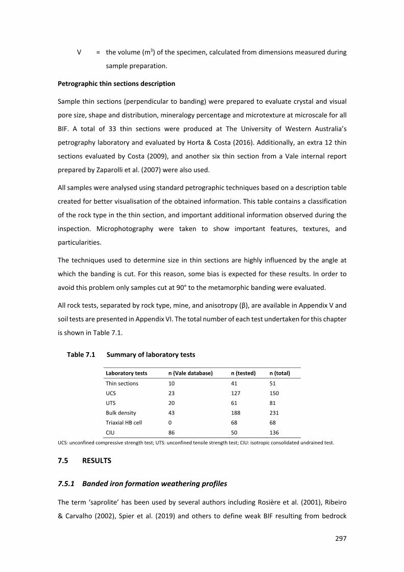
297
V = the volume (m3) of the specimen, calculated from dimensions measured during
sample preparation.
Petrographic thin sections description
Sample thin sections (perpendicular to banding) were prepared to evaluate crystal and visual
pore size, shape and distribution, mineralogy percentage and microtexture at microscale for all
BIF. A total of 33 thin sections were produced at The University of Western Australia’s
petrography laboratory and evaluated by Horta & Costa (2016). Additionally, an extra 12 thin
sections evaluated by Costa (2009), and another six thin section from a Vale internal report
prepared by Zaparolli et al. (2007) were also used.
All samples were analysed using standard petrographic techniques based on a description table
created for better visualisation of the obtained information. This table contains a classification
of the rock type in the thin section, and important additional information observed during the
inspection. Microphotography were taken to show important features, textures, and
particularities.
The techniques used to determine size in thin sections are highly influenced by the angle at
which the banding is cut. For this reason, some bias is expected for these results. In order to
avoid this problem only samples cut at 90° to the metamorphic banding were evaluated.
All rock tests, separated by rock type, mine, and anisotropy (β), are available in Appendix V and
soil tests are presented in Appendix VI. The total number of each test undertaken for this chapter
is shown in Table 7.1.
24 Table 7.1 Summary of laboratory tests
Laboratory tests n (Vale database) n (tested) n (total)
Thin sections 10 41 51
UCS 23 127 150
UTS 20 61 81
Bulk density 43 188 231
Triaxial HB cell 0 68 68
CIU 86 50 136
UCS: unconfined compressive strength test; UTS: unconfined tensile strength test; CIU: isotropic consolidated undrained test.
7.5 RESULTS
7.5.1 Banded iron formation weathering profiles
The term ‘saprolite’ has been used by several authors including Rosière et al. (2001), Ribeiro
& Carvalho (2002), Spier et al. (2019) and others to define weak BIF resulting from bedrock
298
weathering, while preserving the original fabric. This terminology is supported by the presence
in weathered variants of typical macro and micromorphological characteristics that are also
observed in fresh BIF lithotypes. The main characteristics observed are specific fabric and
mineralogical changes; development of total porosity; presence of kaolinite and gibbsite; iron
oxides accumulation in fissures and voids; amphibolite alteration to an iron oxide pseudomorph;
fissures and evidence of dissolution of quartz. In addition, there can be homogenisation of the
banding heterogeneity induced by dissolution of iron dolomite and quartz and collapse of voids
brecciating the original proto-ore fabric. Ultimately, a residual soil with ISRM (1981) weathering
class W6 (ochreous goethitic itabirite) shows disappearance of the original fabric with
homogenisation of the rock mass, changes in colour and clay enrichment with shrink-swell
shearing behaviour.
Based on these characteristics it was possible to separate various BIF types by mineralogical
composition (lithotype) and the degree of weathering, and subsequently associate the materials
with estimated UCS ranges for different geomechanical classifications, based on Martin & Stacey
(2018) proposed table plotted in Figure 7.17.
Following the weathering classification suggested by ISRM (1981) the materials in this study
have the following grouping associated with the weathering horizons profile as suggested by
Deere & Patton (1971):
• FDI, FAI and FQI: bedrock, represent the typical metamorphic banding with minor
influence of supergenic or weathering processes, defined as proto-ore or fresh to
slightly weathered BIF (W1 and W2), with high UCS ranging from 100 MPa to 520 MPa
(light green dashed square in Figure 7.17).
• PWQI and PWGI: saprocks, partially affected by supergenic or weathering processes,
defined as moderately weathered materials (W3) with intermediate intact rock UCS
ranging from 1 MPa to 200 MPa (blue dashed square in Figure 7.17).
• WHE, WAI, WGI and WQI: weak rocks, totally affected by supergenic or weathering
processes, defining the highly to completely weathered BIF (W4 and W5) with low UCS
ranging from 0.05 MPa to 2.5 MPa (red dashed square in Figure 7.17).
• HHE and MHE are hard to medium strength hematitite material, the genesis of these
lithotypes is primarily associated with tectonic metamorphic events and or hypogenic
iron enrichment. For this reason, they are poorly affected by supergenic and
weathering process and are presented in different columns in Figure 7.17.
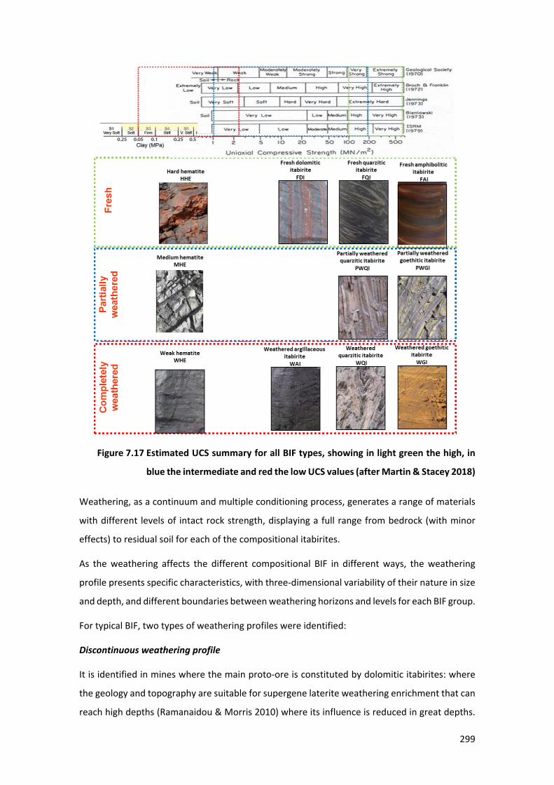
299
100 Figure 7.17 Estimated UCS summary for all BIF types, showing in light green the high, in
blue the intermediate and red the low UCS values (after Martin & Stacey 2018)
Weathering, as a continuum and multiple conditioning process, generates a range of materials
with different levels of intact rock strength, displaying a full range from bedrock (with minor
effects) to residual soil for each of the compositional itabirites.
As the weathering affects the different compositional BIF in different ways, the weathering
profile presents specific characteristics, with three-dimensional variability of their nature in size
and depth, and different boundaries between weathering horizons and levels for each BIF group.
For typical BIF, two types of weathering profiles were identified:
Discontinuous weathering profile
It is identified in mines where the main proto-ore is constituted by dolomitic itabirites: where
the geology and topography are suitable for supergene laterite weathering enrichment that can
reach high depths (Ramanaidou & Morris 2010) where its influence is reduced in great depths.
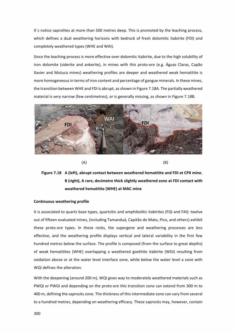
300
It´s notice saprolites at more than 500 metres deep. This is promoted by the leaching process,
which defines a dual weathering horizons with bedrock of fresh dolomitic itabirite (FDI) and
completely weathered types (WHE and WAI).
Since the leaching process is more effective over dolomitic itabirite, due to the high solubility of
iron dolomite (siderite and ankerite), in mines with this proto-ore (e.g. Águas Claras, Capão
Xavier and Mutuca mines) weathering profiles are deeper and weathered weak hematitite is
more homogeneous in terms of iron content and percentage of gangue minerals. In these mines,
the transition between WHE and FDI is abrupt, as shown in Figure 7.18A. The partially weathered
material is very narrow (few centimetres), or is generally missing, as shown in Figure 7.18B.
(A) (B)
101 Figure 7.18 A (left), abrupt contact between weathered hematitite and FDI at CPX mine.
B (right), A rare, decimetre thick slightly weathered zone at FDI contact with
weathered hematitite (WHE) at MAC mine
Continuous weathering profile
It is associated to quartz base types, quartzitic and amphibolitic itabirites (FQI and FAI): twelve
out of fifteen evaluated mines, (including Tamanduá, Capitão do Mato, Pico, and others) exhibit
these proto-ore types. In these rocks, the supergene and weathering processes are less
effective, and the weathering profile displays vertical and lateral variability in the first few
hundred metres below the surface. The profile is composed (from the surface to great depths)
of weak hematitites (WHE) overlapping a weathered goethite itabirite (WGI) resulting from
oxidation above or at the water level interface zone, while below the water level a zone with
WQI defines the alteration.
With the deepening (around 200 m), WQI gives way to moderately weathered materials such as
PWQI or PWGI and depending on the proto-ore this transition zone can extend from 300 m to
400 m, defining the saprocks zone. The thickness of this intermediate zone can vary from several
to a hundred metres, depending on weathering efficacy. These saprocks may, however, contain
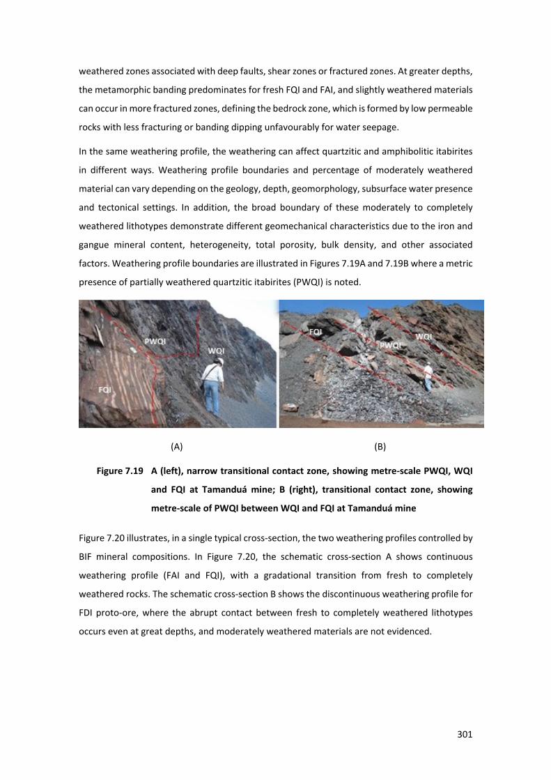
301
weathered zones associated with deep faults, shear zones or fractured zones. At greater depths,
the metamorphic banding predominates for fresh FQI and FAI, and slightly weathered materials
can occur in more fractured zones, defining the bedrock zone, which is formed by low permeable
rocks with less fracturing or banding dipping unfavourably for water seepage.
In the same weathering profile, the weathering can affect quartzitic and amphibolitic itabirites
in different ways. Weathering profile boundaries and percentage of moderately weathered
material can vary depending on the geology, depth, geomorphology, subsurface water presence
and tectonical settings. In addition, the broad boundary of these moderately to completely
weathered lithotypes demonstrate different geomechanical characteristics due to the iron and
gangue mineral content, heterogeneity, total porosity, bulk density, and other associated
factors. Weathering profile boundaries are illustrated in Figures 7.19A and 7.19B where a metric
presence of partially weathered quartzitic itabirites (PWQI) is noted.
(A) (B)
102 Figure 7.19 A (left), narrow transitional contact zone, showing metre-scale PWQI, WQI
and FQI at Tamanduá mine; B (right), transitional contact zone, showing
metre-scale of PWQI between WQI and FQI at Tamanduá mine
Figure 7.20 illustrates, in a single typical cross-section, the two weathering profiles controlled by
BIF mineral compositions. In Figure 7.20, the schematic cross-section A shows continuous
weathering profile (FAI and FQI), with a gradational transition from fresh to completely
weathered rocks. The schematic cross-section B shows the discontinuous weathering profile for
FDI proto-ore, where the abrupt contact between fresh to completely weathered lithotypes
occurs even at great depths, and moderately weathered materials are not evidenced.
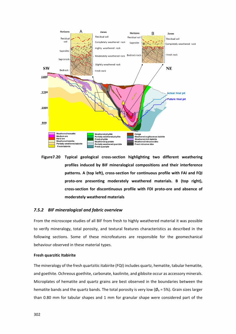
302
103 Figure7.20 Typical geological cross-section highlighting two different weathering
profiles induced by BIF mineralogical compositions and their interference
patterns. A (top left), cross-section for continuous profile with FAI and FQI
proto-ore presenting moderately weathered materials. B (top right),
cross-section for discontinuous profile with FDI proto-ore and absence of
moderately weathered materials
7.5.2 BIF mineralogical and fabric overview
From the microscope studies of all BIF from fresh to highly weathered material it was possible
to verify mineralogy, total porosity, and textural features characteristics as described in the
following sections. Some of these microfeatures are responsible for the geomechanical
behaviour observed in these material types.
Fresh quarzitic Itabirite
The mineralogy of the fresh quartzitic itabirite (FQI) includes quartz, hematite, tabular hematite,
and goethite. Ochreous goethite, carbonate, kaolinite, and gibbsite occur as accessory minerals.
Microplates of hematite and quartz grains are best observed in the boundaries between the
hematite bands and the quartz bands. The total porosity is very low (Øb = 5%). Grain sizes larger
than 0.80 mm for tabular shapes and 1 mm for granular shape were considered part of the
303
hematite band. Goethite appears as small crystals and, in the quartz rich areas, anhedral forms
can also occur. Bands of quartz have low total porosity, which mainly takes the shape of
intergranular total porosity. However, in the layers where microplates of hematite occur in
larger quantity with quartz, the porosity is usually slightly greater. Hematite grains larger than
1.3 mm were considered part of the banding itself.
Moderately weathered quartzitic itabirite
The predominant mineralogy in the moderately weathered, denominated partially weathered
quartzitic itabirite (PWQI) are hematite, quartz, ochreous goethite, goethite, kaolinite, and
gibbsite. Hematite is characterised by grains with low intergranular porosity. Some pores can be
partially/completely filled with goethite or ochreous goethite, and goethite can also occur as a
cement between grains. In general, kaolinite and gibbsite appear as a filling in intragranular
pores. Quartz bands and hematite bands can occur, with the preserved hematite bands are
mainly characterised by serriform contact between hematite grains; visual total porosity can
reach high percentages (20% to 30%).
Total porosity is lower where tabular hematite is predominant. Secondary porosity is mainly
characterised by fractures varying in width between 0.01 mm to 0.24 mm.
Weathered quartzitic itabirite
The highly to completely weathered quartzitic itabirite (WQI) is composed of granular and
tabular hematite, goethite, and ochreous goethite bands interbedded with quartz, goethite,
ochreous goethite kaolinite and gibbsite bands. WQI exhibits a high visual total porosity
normally varying from 25% to 30%, with pore sizes varying from 0.1 mm to 0.25 mm.
Anhedral hematite usually occurs as large crystals (2 mm) and the remaining tabular hematite is
concentrated at iron bands boundaries. Intragranular are associated with granular hematite,
often filled with goethite.
Fresh amphibolitic itabirite
The mineralogy of fresh amphibolitic itabirite (FAI) is mainly defined by quartz, hematite,
pseudomorphs of amphibolite, goethite, and ochreous goethite. The pseudomorphs of
amphibolite are generally altered to fibrous goethite which only occur in some of the thin
sections, where it is very often observed in the boundaries of the iron bands. Goethite usually
occurs in anhedral shape between quartz grains as a cement, but also in a smaller amount as
crystals. Quartz bands are well preserved, and large hematite crystals were interpreted as part
of the preserved hematite bands. The hematite exhibits low visual total porosity (Øb = 5%), as
304
does the quartz. Hematite occurs mainly as granular grains, while the bands show varying
degrees of preservation, from poorly preserved to well preserved. In some cases, the limits
between quartz and hematite bands are not very clear. All the samples exhibit low visual total
porosity.
Moderately weathered goethitic itabirite
The moderately weathered type, referred to as partially weathered goethitic itabirite (PWGI) is
characterised by hematite, goethite, and quartz, with ochreous goethite, gibbsite and kaolinite
occurring in smaller percentages. Anhedral crystalline goethite crystals are also commonly
observed in smaller concentrations, while goethite cement is present filling spaces between
grains of quartz and hematite. Hematite is present as grains and microplates, usually with
serriform contact and have a high visual total porosity usually varying between 15% and 30%.
Preserved banding is observed in most of the thin sections. Some quartz bands have a low total
porosity, with goethite as a cement filling the space in between the grains of quartz and
hematite and, less commonly, as small grains (size in between 0.005 mm to 0.02 mm). The bands
of hematite are mainly characterised by grains of hematite with an intergranular porosity equal
to 15%. Tabular grains also occur as microplates of hematite in the boundaries of the bands.
Fractures (with widths of between 0.10 mm to 0.2mm) occur and can be partially filled with
goethite and ochreous goethite.
Weathered goethite itabirite
The highly to completely weathered goethitic itabirite (WGI) is composed of goethite, hematite,
granular quartz and ochreous goethite. Hematite occurs as microplates and small granular
grains, and larger granular grains are also present.
Hematite banding is preserved and is defined by the remaining hematite grains interbedded
with goethite, ochreous goethite and quartz bands. Total visual porosity is high (15% to 30%),
with intergranular pores usually associated with iron-rich bands and the larger granular grains
of hematite.
Fresh dolomitic itabirite
The mineralogy of the fresh dolomitic itabirite (FDI) is defined by hematite, iron dolomite, quartz
and goethite. Granular hematite is predominant, and its grain size is decreased when iron
dolomites (ankerite and siderite) occur in higher quantities. The iron dolomites occur interlayered
with hematite bands, as well as filling spaces between granuloblastic hematite grains.
305
Carbonate (calcite) occurs as cement and veins, filling spaces between grains of hematite and
iron dolomites; its occurrence is more common at the boundaries of hematite bands where iron
dolomite and hematite grains of smaller size dominate the scene. Anhedral goethite can also
occur in these areas, but its occurrence is limited, and most of the goethite occurs in the shape
of grains in and adjacent to bands of hematite.
Quartz is present in bands with oriented grains and partial grains. Talc and sericite occur as
accessory minerals. Bands of hematite and iron dolomite are still preserved, characterised by
low porosity. When bands are not preserved, hematite occurs as grains, with very fine-grained
iron dolomite as the matrix. The percentage of pores is generally limited, although intergranular
pores size is considerably larger when associated with carbonate. The small presence of
intragranular pores is mostly linked to grains of hematite.
Weathered argillaceous itabirite
Highly to completely weathered argillaceous itabirite (WAI) is mineralogically composed of
granular hematite and microplates of hematite, ochreous goethite, goethite, gibbsite and
kaolinite and granular quartz and exhibits Øb = 30%. The hematite bands show Øb varying from
10% to 30% as defined by Zaparolli et al. (2007), due to secondary cementing of the voids.
Anisotropy is defined by the orientation of tabular and granular hematite, with grain sizes larger
than 0.5 mm. Specular hematites occur as accessory minerals.
Ochreous goethite is the most common cement, but hematite can also act in that role, filling the
spaces between hematite grains. Goethite usually occurs in an anhedral form, but aggregates
are also present in smaller concentrations and grain sizes. Iron bands can present large granular
hematite crystals (>1 mm).
Weak hematitite
Weak hematitite (WHE) consists of hematite and martite, showing heterogeneity defined by
lamellar iron minerals such as specularite (0.07 mm long and 0.01 mm wide), or of martite and
hematite microplates growing over a granoblastic fabric (0.024 mm to 1.2 mm).
More oriented bands are defined by small tabular hematite (0.05 mm long and 0.01 mm wide)
Granular hematite sections bands show variations in size, with visual total porosity (10% to 25%),
as described by Costa (2009), and shown in Figure 7.7B. These porous layers are interconnected
in some areas that are more leached or altered, defining weaker zones, depending on the
weathering intensity.
306
Table 7.2 shows summary results for 51 thin sections presenting the name and percentage of
the main constituent minerals, and maximum and minimum crystal size (between brackets).
Also presented are the percentage, and maximum and minimum size (between brackets) of
pores for three different types of visual measures. Intragranular pores correspond with the
percentage of pores inside crystals that can or cannot be interconnected. Intergranular pores
correspond with visual total porosity between crystals and are generally interconnected.
Secondary pores refer to fracture pore percentage. Visual total porosity is the sum of the three
pore percentages and is considered the maximum total percentage. For total porosity in
brackets, the minimum value did not consider the secondary pores (intact rock) and for
maximum value, the secondary pore is included.
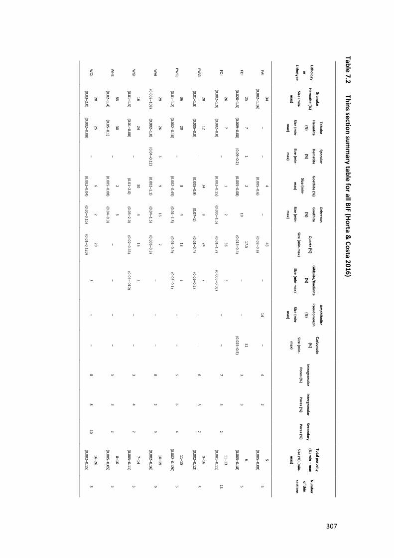
25 Table 7.2 Thins section sum
mary table for all BIF (H
orta & Costa 2016)
Lithology
or
Lithotype
Granular
Hematite (%
)
Size (min-
max)
Tabular
Hematite
(%)
Size (min-
max)
Specular
Hematite
(%)
Size (min-
max)
Goethite (%
)
Size (min-
max)
Ochreous
Goethite
(%)
Size (min-
max)
Quartz (%
)
Size (min-m
ax)
Gibbsite/Kaolinite
(%)
Size (min-m
ax)
Amphibolite
Pseudomorph
(%)
Size (min-
max)
Carbonate
(%)
Size (min-
max)
Intragranular
Pores (%)
Intergranular
Pores (%)
Secondary
Pores (%)
Total porosity
(%) m
in – max
Size (%) (m
in-
max)
Num
ber
of thin
sections
FAI 34
(0.002–1.16) –
– 4
(0.005–0.6) –
43
(0.02–0.8) –
14 –
42
5
(0. 005–0.08) 5
FDI 25
(0.020–1.5)
7
(0.009–0.08)
1
(0.09–0.2)
2
(0.005–0.08) 10
17.5
(0.015–0.4) –
– 32
(0.025–0.5) 3
3 6
(0.005–0.18) 5
FQI
26
(0.002–1.9)
7
(0.002–0.8) –
1
(0.002–0.15)
2
(0.005–1.5)
36
(0.01–1.7)
5
(0.005–0.03) –
– 7
4 2
11–13
(0.001–0.11) 13
PWGI
28
(0.01–1.8)
12
(0.005–0.8) –
34
(0.005–0.9)
8
(0.07–1)
24
(0.01–0.4)
2
(0.06–0.2) –
– 6
3 7
9–16
(0.002–0.12) 5
PWQ
I 36
(0.01–1.2)
20
(0.002–0.10) –
8
(0.002–0.45)
4
(0.01–1.5)
18
(0.01–0.9)
2
(0.03–0.1) –
– 5
6 4
11–15
(0.002–0.120) 5
WAI
29
(0.002–108)
26
(0.002–1.0)
3
(0.04–0.12)
9
(0.002–1.1)
15
(0.04–1.5)
7
(0.006–0.3) –
– –
8 2
9 10–19
(0.002–0.16) 9
WGI
16
(0.01–1.5)
24
(0.01–0.08) –
30
(0.01–2.0)
4
(0.05–2.0)
16
(0.02–0.45)
3
(0.03–.010) –
– 3
4 7
7–14
(0.005–0.11) 3
WHE
55
(0.02–1.4)
30
(0.05–0.1) –
2
(0.005–0.08)
3
(0.04–0.3) –
– –
– 5
3 2
8–10
(0.005–0.05) 3
WQ
I 28
(0.03–2.0)
25
(0.002–0.08) –
6
(0.002–0.04)
2
(0.05–0.15)
20
(0.01–0.120) 3
– –
8 8
10 16–26
(0.002–0.15) 3
307
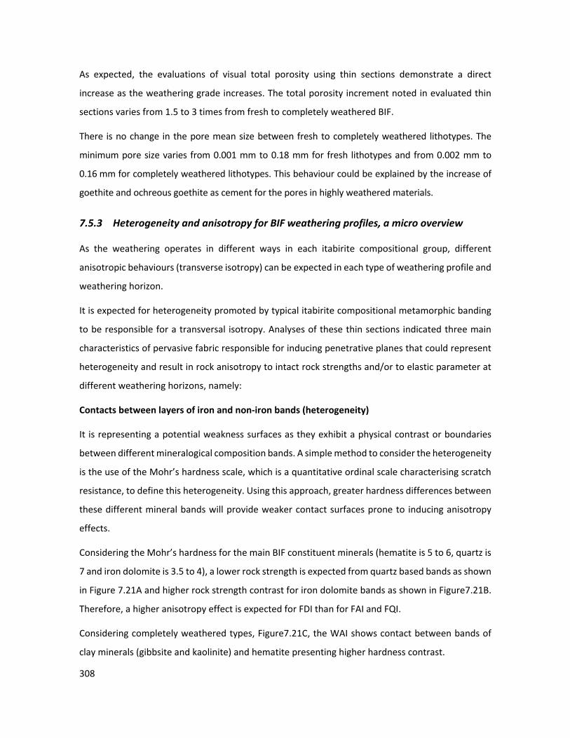
308
As expected, the evaluations of visual total porosity using thin sections demonstrate a direct
increase as the weathering grade increases. The total porosity increment noted in evaluated thin
sections varies from 1.5 to 3 times from fresh to completely weathered BIF.
There is no change in the pore mean size between fresh to completely weathered lithotypes. The
minimum pore size varies from 0.001 mm to 0.18 mm for fresh lithotypes and from 0.002 mm to
0.16 mm for completely weathered lithotypes. This behaviour could be explained by the increase of
goethite and ochreous goethite as cement for the pores in highly weathered materials.
7.5.3 Heterogeneity and anisotropy for BIF weathering profiles, a micro overview
As the weathering operates in different ways in each itabirite compositional group, different
anisotropic behaviours (transverse isotropy) can be expected in each type of weathering profile and
weathering horizon.
It is expected for heterogeneity promoted by typical itabirite compositional metamorphic banding
to be responsible for a transversal isotropy. Analyses of these thin sections indicated three main
characteristics of pervasive fabric responsible for inducing penetrative planes that could represent
heterogeneity and result in rock anisotropy to intact rock strengths and/or to elastic parameter at
different weathering horizons, namely:
Contacts between layers of iron and non-iron bands (heterogeneity)
It is representing a potential weakness surfaces as they exhibit a physical contrast or boundaries
between different mineralogical composition bands. A simple method to consider the heterogeneity
is the use of the Mohr’s hardness scale, which is a quantitative ordinal scale characterising scratch
resistance, to define this heterogeneity. Using this approach, greater hardness differences between
these different mineral bands will provide weaker contact surfaces prone to inducing anisotropy
effects.
Considering the Mohr’s hardness for the main BIF constituent minerals (hematite is 5 to 6, quartz is
7 and iron dolomite is 3.5 to 4), a lower rock strength is expected from quartz based bands as shown
in Figure 7.21A and higher rock strength contrast for iron dolomite bands as shown in Figure7.21B.
Therefore, a higher anisotropy effect is expected for FDI than for FAI and FQI.
Considering completely weathered types, Figure7.21C, the WAI shows contact between bands of
clay minerals (gibbsite and kaolinite) and hematite presenting higher hardness contrast.
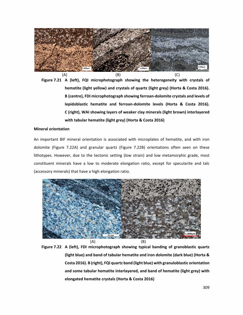
309
(A) (B) (C) 104 Figure 7.21 A (left), FQI microphotograph showing the heterogeneity with crystals of
hematite (light yellow) and crystals of quartz (light grey) (Horta & Costa 2016).
B (centre), FDI microphotograph showing ferroan-dolomite crystals and levels of
lepidoblastic hematite and ferroan-dolomite levels (Horta & Costa 2016).
C (right), WAI showing layers of weaker clay minerals (light brown) interlayered
with tabular hematite (light grey) (Horta & Costa 2016)
Mineral orientation
An important BIF mineral orientation is associated with microplates of hematite, and with iron
dolomite (Figure 7.22A) and granular quartz (Figure 7.22B) orientations often seen on these
lithotypes. However, due to the tectonic setting (low strain) and low metamorphic grade, most
constituent minerals have a low to moderate elongation ratio, except for specularite and talc
(accessory minerals) that have a high elongation ratio.
(A) (B) 105 Figure 7.22 A (left), FDI microphotograph showing typical banding of granoblastic quartz
(light blue) and band of tabular hematite and iron dolomite (dark blue) (Horta &
Costa 2016). B (right), FQI quartz band (light blue) with granuloblastic orientation
and some tabular hematite interlayered, and band of hematite (light grey) with
elongated hematite crystals (Horta & Costa 2016)
1,000μm
1,000μm 1,000μm
1,000μm
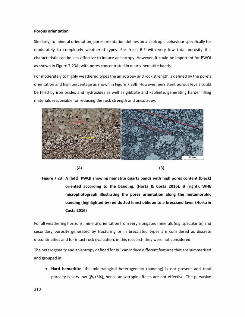
310
Porous orientation
Similarly, to mineral orientation, pores orientation defines an anisotropic behaviour specifically for
moderately to completely weathered types. For fresh BIF with very low total porosity this
characteristic can be less effective to induce anisotropy. However, it could be important for PWQI
as shown in Figure 7.23A, with pores concentrated in quartz hematite bands.
For moderately to highly weathered types the anisotropy and rock strength is defined by the pore’s
orientation and high percentage as shown in Figure 7.23B. However, persistent porous levels could
be filled by iron oxides and hydroxides as well as gibbsite and kaolinite, generating harder filling
materials responsible for reducing the rock strength and anisotropy.
(A) (B)
106 Figure 7.23 A (left), PWQI showing hematite quartz bands with high pores content (black)
oriented according to the banding. (Horta & Costa 2016). B (right), WHE
microphotograph illustrating the pores orientation along the metamorphic
banding (highlighted by red dotted lines) oblique to a brecciaed layer (Horta &
Costa 2016)
For all weathering horizons, mineral orientation from very elongated minerals (e.g. specularite) and
secondary porosity generated by fracturing or in brecciated types are considered as discrete
discontinuities and for intact rock evaluation, in this research they were not considered.
The heterogeneity and anisotropy defined for BIF can induce different features that are summarised
and grouped in:
• Hard hematitite: the mineralogical heterogeneity (banding) is not present and total
porosity is very low (Øb<5%), hence anisotropic effects are not effective. The pervasive
1000μm
A
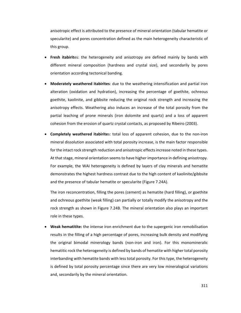
311
anisotropic effect is attributed to the presence of mineral orientation (tabular hematite or
specularite) and pores concentration defined as the main heterogeneity characteristic of
this group.
• Fresh itabirites: the heterogeneity and anisotropy are defined mainly by bands with
different mineral composition (hardness and crystal size), and secondarily by pores
orientation according tectonical banding.
• Moderately weathered itabirites: due to the weathering intensification and partial iron
alteration (oxidation and hydration), increasing the percentage of goethite, ochreous
goethite, kaolinite, and gibbsite reducing the original rock strength and increasing the
anisotropy effects. Weathering also induces an increase of the total porosity from the
partial leaching of prone minerals (iron dolomite and quartz) and a loss of apparent
cohesion from the erosion of quartz crystal contacts, as proposed by Ribeiro (2003).
• Completely weathered itabirites: total loss of apparent cohesion, due to the non-iron
mineral dissolution associated with total porosity increase, is the main factor responsible
for the intact rock strength reduction and anisotropic effects increase noted in these types.
At that stage, mineral orientation seems to have higher importance in defining anisotropy.
For example, the WAI heterogeneity is defined by layers of clay minerals and hematite
demonstrates the highest hardness contrast due to the high content of kaolinite/gibbsite
and the presence of tabular hematite or specularite (Figure 7.24A).
The iron reconcentration, filling the pores (cement) as hematite (hard filling), or goethite
and ochreous goethite (weak filling) can partially or totally modify the anisotropy and the
rock strength as shown in Figure 7.24B. The mineral orientation also plays an important
role in these types.
• Weak hematitite: the intense iron enrichment due to the supergenic iron remobilisation
results in the filling of a high percentage of pores, increasing bulk density and modifying
the original bimodal minerology bands (non-iron and iron). For this monomineralic
hematitic rock the heterogeneity is defined by bands of hematite with higher total porosity
interbanding with hematite bands with less total porosity. For this type, the heterogeneity
is defined by total porosity percentage since there are very low mineralogical variations
and, secondarily by the mineral orientation.
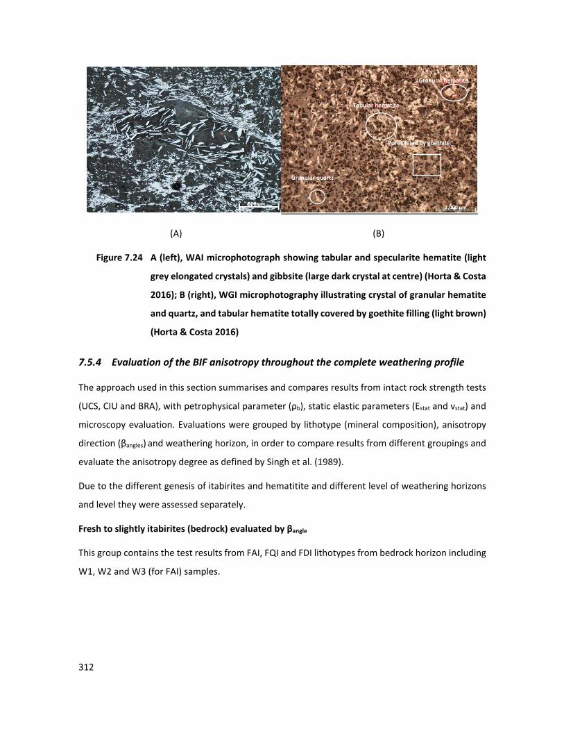
312
(A) (B)
107 Figure 7.24 A (left), WAI microphotograph showing tabular and specularite hematite (light
grey elongated crystals) and gibbsite (large dark crystal at centre) (Horta & Costa
2016); B (right), WGI microphotography illustrating crystal of granular hematite
and quartz, and tabular hematite totally covered by goethite filling (light brown)
(Horta & Costa 2016)
7.5.4 Evaluation of the BIF anisotropy throughout the complete weathering profile
The approach used in this section summarises and compares results from intact rock strength tests
(UCS, CIU and BRA), with petrophysical parameter (ρb), static elastic parameters (Estat and νstat) and
microscopy evaluation. Evaluations were grouped by lithotype (mineral composition), anisotropy
direction (βangles) and weathering horizon, in order to compare results from different groupings and
evaluate the anisotropy degree as defined by Singh et al. (1989).
Due to the different genesis of itabirites and hematitite and different level of weathering horizons
and level they were assessed separately.
Fresh to slightly itabirites (bedrock) evaluated by βangle
This group contains the test results from FAI, FQI and FDI lithotypes from bedrock horizon including
W1, W2 and W3 (for FAI) samples.
Tabular hematite
Granular hematite
Granular quartz
Pores filled by goethite
500 μm 1,000 μm
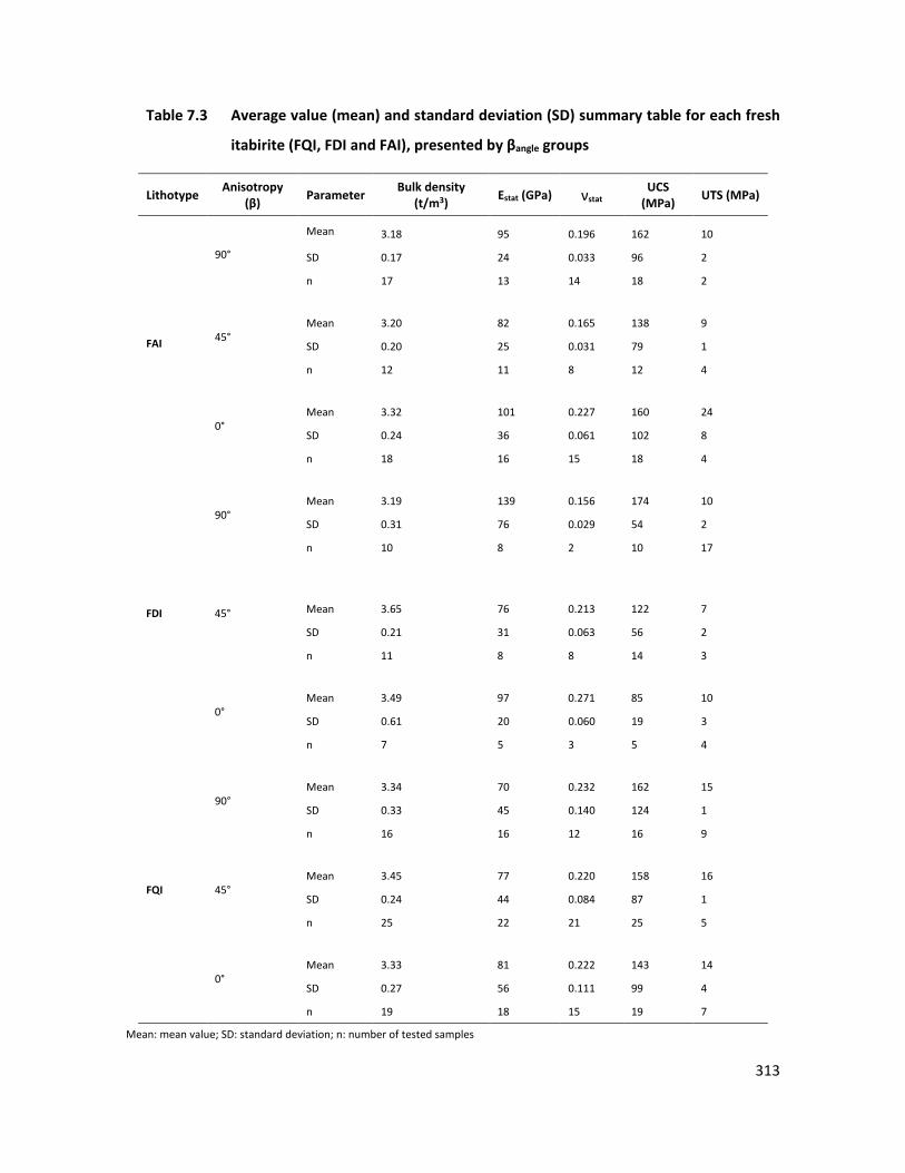
313
26 Table 7.3 Average value (mean) and standard deviation (SD) summary table for each fresh
itabirite (FQI, FDI and FAI), presented by βangle groups
Lithotype Anisotropy (β) Parameter Bulk density
(t/m3) Estat (GPa) νstat UCS
(MPa) UTS (MPa)
FAI
90°
Mean 3.18 95 0.196 162 10
SD 0.17 24 0.033 96 2
n 17 13 14 18 2
45°
Mean 3.20 82 0.165 138 9
SD 0.20 25 0.031 79 1
n 12 11 8 12 4
0°
Mean 3.32 101 0.227 160 24
SD 0.24 36 0.061 102 8
n 18 16 15 18 4
FDI
90°
Mean 3.19 139 0.156 174 10
SD 0.31 76 0.029 54 2
n 10 8 2 10 17
45°
Mean 3.65 76 0.213 122 7
SD 0.21 31 0.063 56 2
n 11 8 8 14 3
0°
Mean 3.49 97 0.271 85 10
SD 0.61 20 0.060 19 3
n 7 5 3 5 4
FQI
90°
Mean 3.34 70 0.232 162 15
SD 0.33 45 0.140 124 1
n 16 16 12 16 9
45°
Mean 3.45 77 0.220 158 16
SD 0.24 44 0.084 87 1
n 25 22 21 25 5
0°
Mean 3.33 81 0.222 143 14
SD 0.27 56 0.111 99 4
n 19 18 15 19 7
Mean: mean value; SD: standard deviation; n: number of tested samples
314
From Table 7.3 it is possible to note that:
• Bulk density results show similar means, with a higher mean value obtained for FDI β45° =
3.65 t/m3 ±0.21 t/m3 and a lower value for FAI β45° = 3.18 t/m3 ±0.17 t/m3, showing means
raging within the SD. Higher ρb values were obtained for FDI, showing also the highest
range between different Bangles.
• Static Young’s modulus means presented the higher mean value for FDI β90° = 139 GPa ±76
GPa and lower value for FQI β90° = 70 GPa ±45 GPa showing the mean of each lithotype is
within the SD range.
• Static Poisson’s ratio presents the higher mean value for FDI β0° = 0.271 ±0.0.06 and lower
value for FDI β90° = 0.156 ±0.029. FAI and FDI present higher means for β0° and FQI showed
similar means for all directions with a higher SD from 0.084 to 0.140.
• UCS tests exhibit the higher mean value for FDI β90° = 174 MPa ±54 MPa and lower value for
FDI β90° = 85 MPa ±19 MPa. The mean of each lithotype is within inside the SD range.
• FAI and FQI present the highest means with lower values for β45°. FDI presented lowest
mean at β0°.
• BRA (UTS) tests show the higher mean value for FAI β0° = 24 MPa ±8 MPa and lower value
for FDI β45° = 7 MPa ±2 MPa. FQI presented similar means for all directions and presented
the highest mean values. FAI and FDI presented lower values at β45°.
Hard hematitite (bedrock) evaluated by βangle
This group contains only HHE with weathering grade equal to W1 and W2. The same approach used
for itabirites was applied for HHE and results are presented in Table 7.4.
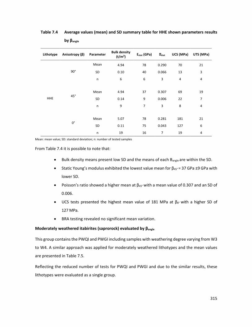
315
27 Table 7.4 Average values (mean) and SD summary table for HHE shown parameters results
by βangle
Lithotype Anisotropy (β) Parameter Bulk density (t/m3) Estat (GPa) stat UCS (MPa) UTS (MPa)
HHE
90°
Mean 4.94 78 0.290 70 21
SD 0.10 40 0.066 13 3
n 6 6 3 4 4
45°
Mean 4.94 37 0.307 69 19
SD 0.14 9 0.006 22 7
n 9 7 3 8 4
0°
Mean 5.07 78 0.281 181 21
SD 0.11 75 0.043 127 6
n 19 16 7 19 4
Mean: mean value; SD: standard deviation; n: number of tested samples
From Table 7.4 it is possible to note that:
• Bulk density means present low SD and the means of each Bangle are within the SD.
• Static Young’s modulus exhibited the lowest value mean for β45° = 37 GPa ±9 GPa with
lower SD.
• Poisson’s ratio showed a higher mean at β45° with a mean value of 0.307 and an SD of
0.006.
• UCS tests presented the highest mean value of 181 MPa at β0° with a higher SD of
127 MPa.
• BRA testing revealed no significant mean variation.
Moderately weathered itabirites (saprorock) evaluated by βangle
This group contains the PWQI and PWGI including samples with weathering degree varying from W3
to W4. A similar approach was applied for moderately weathered lithotypes and the mean values
are presented in Table 7.5.
Reflecting the reduced number of tests for PWQI and PWGI and due to the similar results, these
lithotypes were evaluated as a single group.
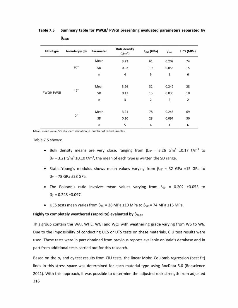
316
28 Table 7.5 Summary table for PWQI/ PWGI presenting evaluated parameters separated by
βangle
Lithotype Anisotropy (β) Parameter Bulk density (t/m3) Estat (GPa) νstat UCS (MPa)
PWQI/ PWGI
90°
Mean 3.23 61 0.202 74
SD 0.02 19 0.055 15
n 4 5 5 6
45°
Mean 3.26 32 0.242 28
SD 0.17 15 0.035 10
n 3 2 2 2
0°
Mean 3.21 78 0.248 69
SD 0.10 28 0.097 30
n 5 4 4 6
Mean: mean value; SD: standard deviation; n: number of tested samples
Table 7.5 shows:
• Bulk density means are very close, ranging from β45° = 3.26 t/m3 ±0.17 t/m3 to
β0° = 3.21 t/m3 ±0.10 t/m3, the mean of each type is written the SD range.
• Static Young’s modulus shows mean values varying from β45° = 32 GPa ±15 GPa to
β0° = 78 GPa ±28 GPa.
• The Poisson’s ratio involves mean values varying from β90° = 0.202 ±0.055 to
β0° = 0.248 ±0.097.
• UCS tests mean varies from β45° = 28 MPa ±10 MPa to β90° = 74 MPa ±15 MPa.
Highly to completely weathered (saprolite) evaluated by βangle
This group contain the WAI, WHE, WGI and WQI with weathering grade varying from W5 to W6.
Due to the impossibility of conducting UCS or UTS tests on these materials, CIU test results were
used. These tests were in part obtained from previous reports available on Vale’s database and in
part from additional tests carried out for this research.
Based on the σ1 and σ3 test results from CIU tests, the linear Mohr–Coulomb regression (best fit)
lines in this stress space was determined for each material type using RocData 5.0 (Rocscience
2021). With this approach, it was possible to determine the adjusted rock strength from adjusted
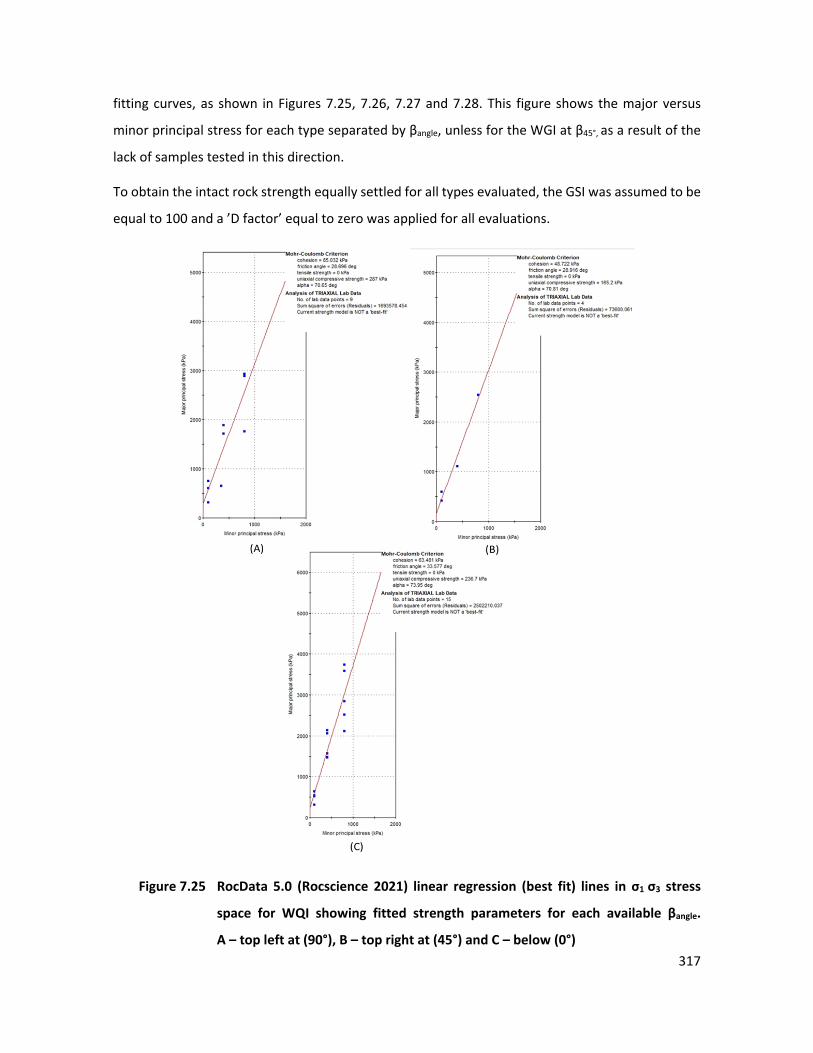
317
fitting curves, as shown in Figures 7.25, 7.26, 7.27 and 7.28. This figure shows the major versus
minor principal stress for each type separated by βangle, unless for the WGI at β45°, as a result of the
lack of samples tested in this direction.
To obtain the intact rock strength equally settled for all types evaluated, the GSI was assumed to be
equal to 100 and a ’D factor’ equal to zero was applied for all evaluations.
108 Figure 7.25 RocData 5.0 (Rocscience 2021) linear regression (best fit) lines in σ1 σ3 stress
space for WQI showing fitted strength parameters for each available βangle.
A – top left at (90°), B – top right at (45°) and C – below (0°)
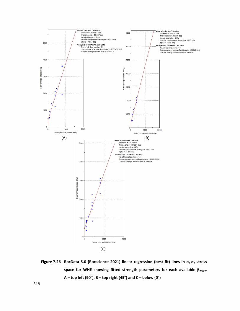
318
109 Figure 7.26 RocData 5.0 (Rocscience 2021) linear regression (best fit) lines in σ1 σ3 stress
space for WHE showing fitted strength parameters for each available βangle.
A – top left (90°), B – top right (45°) and C – below (0°)
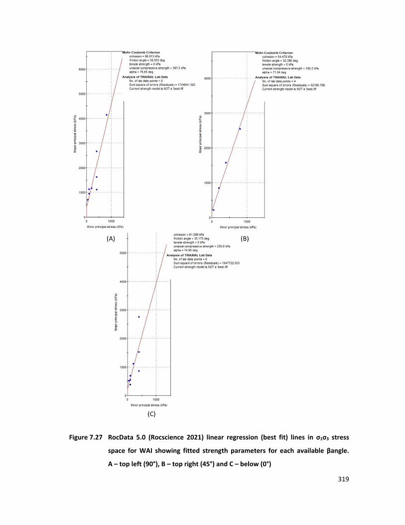
319
u
110 Figure 7.27 RocData 5.0 (Rocscience 2021) linear regression (best fit) lines in σ1σ3 stress
space for WAI showing fitted strength parameters for each available βangle.
A – top left (90°), B – top right (45°) and C – below (0°)
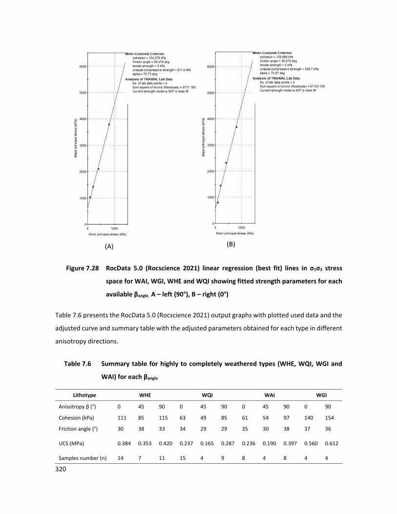
320
111Figure 7.28 RocData 5.0 (Rocscience 2021) linear regression (best fit) lines in σ1σ3 stress
space for WAI, WGI, WHE and WQI showing fitted strength parameters for each
available βangle. A – left (90°), B – right (0°)
Table 7.6 presents the RocData 5.0 (Rocscience 2021) output graphs with plotted used data and the
adjusted curve and summary table with the adjusted parameters obtained for each type in different
anisotropy directions.
29 Table 7.6 Summary table for highly to completely weathered types (WHE, WQI, WGI and
WAI) for each βangle
Lithotype WHE WQI WAI WGI
Anisotropy β (°) 0 45 90 0 45 90 0 45 90 0 90
Cohesion (kPa) 111 85 115 63 49 85 61 54 97 140 154
Friction angle (°) 30 38 33 34 29 29 35 30 38 37 36
UCS (MPa) 0.384 0.353 0.420 0.237 0.165 0.287 0.236 0.190 0.397 0.560 0.612
Samples number (n) 14 7 11 15 4 9 8 4 8 4 4
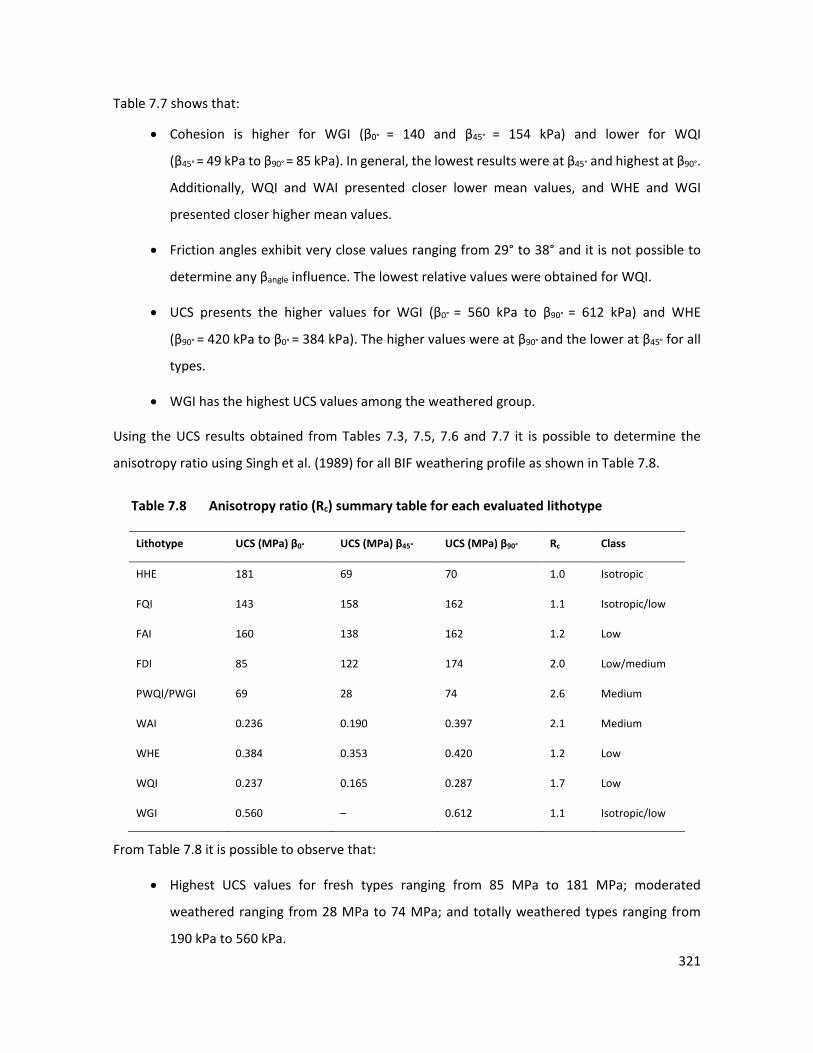
321
Table 7.7 shows that:
• Cohesion is higher for WGI (β0° = 140 and β45° = 154 kPa) and lower for WQI
(β45° = 49 kPa to β90° = 85 kPa). In general, the lowest results were at β45° and highest at β90°.
Additionally, WQI and WAI presented closer lower mean values, and WHE and WGI
presented closer higher mean values.
• Friction angles exhibit very close values ranging from 29° to 38° and it is not possible to
determine any βangle influence. The lowest relative values were obtained for WQI.
• UCS presents the higher values for WGI (β0° = 560 kPa to β90° = 612 kPa) and WHE
(β90° = 420 kPa to β0° = 384 kPa). The higher values were at β90° and the lower at β45° for all
types.
• WGI has the highest UCS values among the weathered group.
Using the UCS results obtained from Tables 7.3, 7.5, 7.6 and 7.7 it is possible to determine the
anisotropy ratio using Singh et al. (1989) for all BIF weathering profile as shown in Table 7.8.
30 Table 7.8 Anisotropy ratio (Rc) summary table for each evaluated lithotype
Lithotype UCS (MPa) β0° UCS (MPa) β45° UCS (MPa) β90° Rc Class
HHE 181 69 70 1.0 Isotropic
FQI 143 158 162 1.1 Isotropic/low
FAI 160 138 162 1.2 Low
FDI 85 122 174 2.0 Low/medium
PWQI/PWGI 69 28 74 2.6 Medium
WAI 0.236 0.190 0.397 2.1 Medium
WHE 0.384 0.353 0.420 1.2 Low
WQI 0.237 0.165 0.287 1.7 Low
WGI 0.560 – 0.612 1.1 Isotropic/low
From Table 7.8 it is possible to observe that:
• Highest UCS values for fresh types ranging from 85 MPa to 181 MPa; moderated
weathered ranging from 28 MPa to 74 MPa; and totally weathered types ranging from
190 kPa to 560 kPa.
322
• The lowest UCS values are concentrated in β45° unless for FQI and FDI where in β0°.
• It is possible to group the anisotropic ratio (Rc) results in two groups (by mineralogical
composition and weathering grade): Isotropic to low Rc (HHE, WHE, FQI, WQI and WGI)
and low to medium Rc (FDI, PWQI/PWGI and WAI).
7.5.5 BIF isotropic approach throughout the complete weathering profile
The anisotropy evaluation in previous sections reveals that, in general, BIF behave as isotropic to
low anisotropy materials; and a second group being FDI and PWQI/ PWGI defined as low to medium
anisotropy ratio. Based on this result, in this section, the BIF were evaluated as isotropic materials
and grouped only by lithotype mineral composition.
RocData 5.0 (Rocscience 2021) was used to support the data manipulation necessary for a general
overview of intact rock strengths and elastic parameters for highly to completely weathered
variants.
Used tables present for each type the mean, SD, covariance (COV), margin of error, maximum values
(Max), minimum values (Min), values of the first and third quartiles (1Qt and 3Qt), lower and upper
inner fences, and number of tested samples (n).
Fresh to slightly weathered itabirites (bedrock) as isotropic material
For this evaluation itabirites were grouped by mineral composition. Table 7.9 shows basic statistical
results for fresh to slightly weathered itabirites (FQI, FDI and FAI).
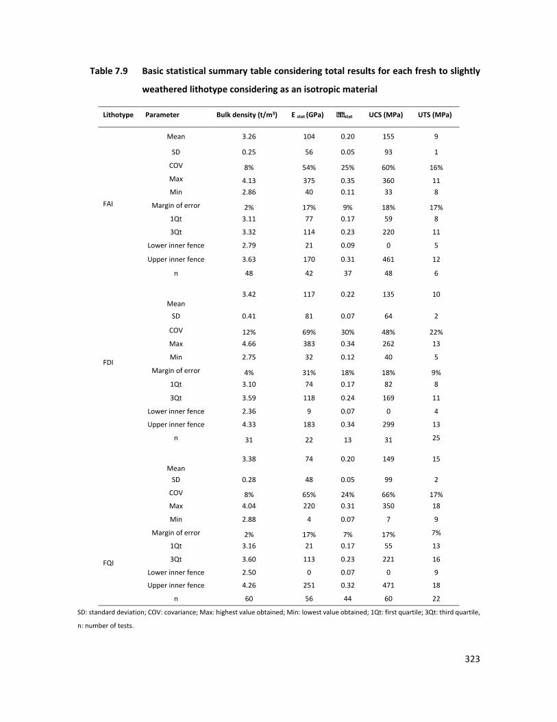
323
31 Table 7.9 Basic statistical summary table considering total results for each fresh to slightly
weathered lithotype considering as an isotropic material
Lithotype Parameter Bulk density (t/m3) E stat (GPa) stat UCS (MPa) UTS (MPa)
FAI
Mean 3.26 104 0.20 155 9
SD 0.25 56 0.05 93 1
COV 8% 54% 25% 60% 16% Max 4.13 375 0.35 360 11 Min 2.86 40 0.11 33 8
Margin of error 2% 17% 9% 18% 17% 1Qt 3.11 77 0.17 59 8
3Qt 3.32 114 0.23 220 11
Lower inner fence 2.79 21 0.09 0 5
Upper inner fence 3.63 170 0.31 461 12
n 48 42 37 48 6
FDI
Mean 3.42 117 0.22 135 10
SD 0.41 81 0.07 64 2
COV 12% 69% 30% 48% 22% Max 4.66 383 0.34 262 13
Min 2.75 32 0.12 40 5
Margin of error 4% 31% 18% 18% 9% 1Qt 3.10 74 0.17 82 8
3Qt 3.59 118 0.24 169 11
Lower inner fence 2.36 9 0.07 0 4
Upper inner fence 4.33 183 0.34 299 13
n 31 22 13 31 25
FQI
Mean 3.38 74 0.20 149 15
SD 0.28 48 0.05 99 2
COV 8% 65% 24% 66% 17% Max 4.04 220 0.31 350 18
Min 2.88 4 0.07 7 9
Margin of error 2% 17% 7% 17% 7%
1Qt 3.16 21 0.17 55 13
3Qt 3.60 113 0.23 221 16
Lower inner fence 2.50 0 0.07 0 9
Upper inner fence 4.26 251 0.32 471 18
n 60 56 44 60 22
SD: standard deviation; COV: covariance; Max: highest value obtained; Min: lowest value obtained; 1Qt: first quartile; 3Qt: third quartile,
n: number of tests.
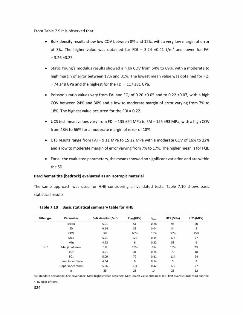
324
From Table 7.9 it is observed that:
• Bulk density results show low COV between 8% and 12%, with a very low margin of error
of 3%. The higher value was obtained for FDI = 3.24 ±0.41 t/m3 and lower for FAI
= 3.26 ±0.25.
• Static Young’s modulus results showed a high COV from 54% to 69%, with a moderate to
high margin of error between 17% and 31%. The lowest mean value was obtained for FQI
= 74 ±48 GPa and the highest for the FDI = 117 ±81 GPa.
• Poisson’s ratio values vary from FAI and FQI of 0.20 ±0.05 and to 0.22 ±0.07, with a high
COV between 24% and 30% and a low to moderate margin of error varying from 7% to
18%. The highest value occurred for the FDI = 0.22.
• UCS test mean values vary from FDI = 135 ±64 MPa to FAI = 155 ±93 MPa, with a high COV
from 48% to 66% for a moderate margin of error of 18%.
• UTS results range from FAI = 9 ±1 MPa to 15 ±2 MPa with a moderate COV of 16% to 22%
and a low to moderate margin of error varying from 7% to 17%. The higher mean is for FQI.
• For all the evaluated parameters, the means showed no significant variation and are within
the SD.
Hard hematitite (bedrock) evaluated as an isotropic material
The same approach was used for HHE considering all validated tests. Table 7.10 shows basic
statistical results.
32 Table 7.10 Basic statistical summary table for HHE
Lithotype Parameter Bulk density (t/m3) E stat (GPa) νstat UCS (MPa) UTS (MPa)
HHE
Mean 5.01 51 0.28 96 20 SD 0.14 33 0.04 34 5
COV 3% 65% 16% 35% 25% Max 5.21 120 0.35 178 27 Min 4.72 6 0.22 55 9
Margin of error 1% 25% 9% 15% 7% 1Qt 4.91 31 0.24 70 18 3Qt 5.09 72 0.31 114 24
Lower inner fence 4.64 0 0.14 5 9 Upper inner fence 5.36 134 0.42 179 27
n 35 28 14 23 12
SD: standard deviation; COV: covariance; Max: highest value obtained; Min: lowest value obtained; 1Qt: first quartile; 3Qt: third quartile,
n: number of tests.
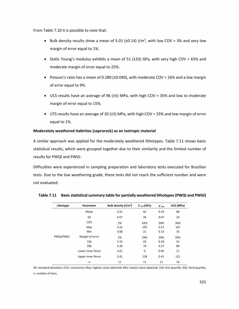
325
From Table 7.10 it is possible to note that:
• Bulk density results show a mean of 5.01 (±0.14) t/m3, with low COV = 3% and very low
margin of error equal to 1%.
• Static Young’s modulus exhibits a mean of 51 (±33) GPa, with very high COV = 65% and
moderate margin of error equal to 25%.
• Poisson’s ratio has a mean of 0.280 (±0.040), with moderate COV = 16% and a low margin
of error equal to 9%.
• UCS results have an average of 96 (±5) MPa, with high COV = 35% and low to moderate
margin of error equal to 15%.
• UTS results have an average of 20 (±5) MPa, with high COV = 25% and low margin of error
equal to 1%.
Moderately weathered itabirites (saprorock) as an isotropic material
A similar approach was applied for the moderately weathered lithotypes. Table 7.11 shows basic
statistical results, which were grouped together due to their similarity and the limited number of
results for PWQI and PWGI.
Difficulties were experienced in sampling preparation and laboratory tests executed for Brazilian
tests. Due to the low weathering grade, these tests did not reach the sufficient number and were
not evaluated.
33 Table 7.11 Basic statistical summary table for partially weathered lithotypes (PWQI and PWGI)
Lithotype Parameter Bulk density (t/m3) E stat (GPa) ν stat UCS (MPa)
PWQI/PWGI
Mean 3.21 62 0.23 68
SD 0.07 26 0.07 23
COV 2% 43% 30% 34% Max 3.31 103 0.37 107 Min 3.08 21 0.13 35
Margin of error 2% 29% 20% 20% 1Qt 3.16 42 0.18 52 3Qt 3.26 76 0.27 80
Lower inner fence 3.01 0 0.05 11
Upper inner fence 3.41 128 0.41 121
n 11 11 11 14
SD: standard deviation; COV: covariance; Max: highest value obtained; Min: lowest value obtained; 1Qt: first quartile; 3Qt: third quartile,
n: number of tests.
326
Table 7.11 shows that:
• Bulk density results showed mean of 3.21 ±0.07 t/m3, with low COV = 2% and very low
margin of error equal to 2%.
• Static Young’s modulus is lower than the other itabirite groups at 62 ±26 GPa, with very
high COV = 43% and moderate to high margin of error equal to 29%.
• Poisson’s ratio is similar to the other itabirite groups at 0.23 ±0.07, with high COV = 30%
and high margin of error equal to 20%.
• UCS results showed mean of 68 ±23 MPa, with high COV = 34% and moderate margin of
error equal to 20%.
Highly to completely weathered itabirites (saprolite) as an isotropic material
For this evaluation, CIU test results were used, based on the tests undertaken for this research and
from the available Vale database.
Based on the σ1 and σ3 test results from CIU tests the linear Mohr–Coulomb regression (best fit)
lines in this stress space was determined for each material type using RocData 5.0 (Rocscience
2021). With this approach, it was possible to determine the adjusted rock strength from adjusted
fitting curves, as shown in Figure 7.29 (A, B, C and D). This figure shows the major versus minor
principal stress for each type (WAI, WQI, WGI and WHE) assuming isotropic materials.
To obtain the intact rock strength equally settled for all types evaluated, the GSI was assumed to be
equal to 100 and a ’D factor’ equal to zero was applied for all evaluations.
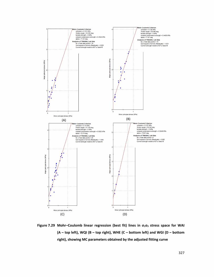
327
112 Figure 7.29 Mohr–Coulomb linear regression (best fit) lines in σ1σ3 stress space for WAI
(A – top left), WQI (B – top right), WHE (C – bottom left) and WGI (D – bottom
right), showing MC parameters obtained by the adjusted fitting curve
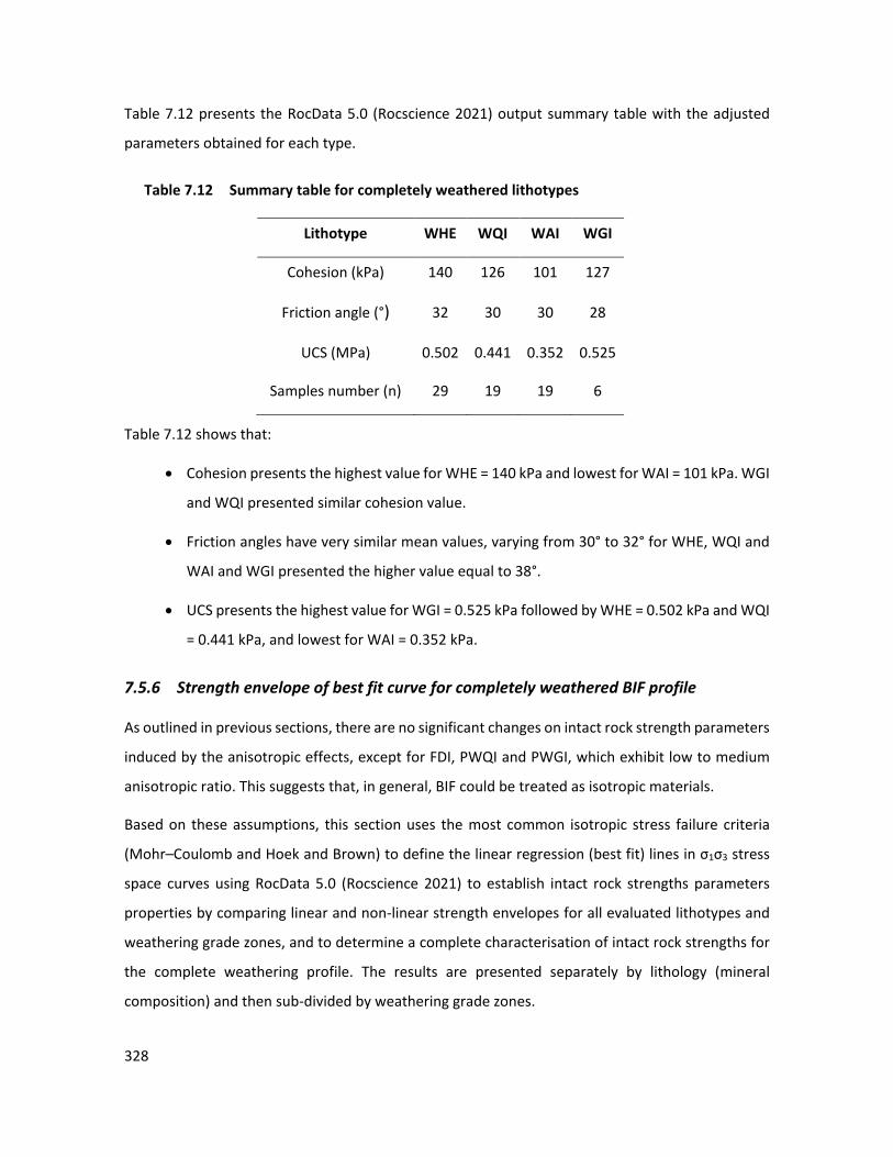
328
Table 7.12 presents the RocData 5.0 (Rocscience 2021) output summary table with the adjusted
parameters obtained for each type.
34 Table 7.12 Summary table for completely weathered lithotypes
Lithotype WHE WQI WAI WGI
Cohesion (kPa) 140 126 101 127
Friction angle (°) 32 30 30 28
UCS (MPa) 0.502 0.441 0.352 0.525
Samples number (n) 29 19 19 6
Table 7.12 shows that:
• Cohesion presents the highest value for WHE = 140 kPa and lowest for WAI = 101 kPa. WGI
and WQI presented similar cohesion value.
• Friction angles have very similar mean values, varying from 30° to 32° for WHE, WQI and
WAI and WGI presented the higher value equal to 38°.
• UCS presents the highest value for WGI = 0.525 kPa followed by WHE = 0.502 kPa and WQI
= 0.441 kPa, and lowest for WAI = 0.352 kPa.
7.5.6 Strength envelope of best fit curve for completely weathered BIF profile
As outlined in previous sections, there are no significant changes on intact rock strength parameters
induced by the anisotropic effects, except for FDI, PWQI and PWGI, which exhibit low to medium
anisotropic ratio. This suggests that, in general, BIF could be treated as isotropic materials.
Based on these assumptions, this section uses the most common isotropic stress failure criteria
(Mohr–Coulomb and Hoek and Brown) to define the linear regression (best fit) lines in σ1σ3 stress
space curves using RocData 5.0 (Rocscience 2021) to establish intact rock strengths parameters
properties by comparing linear and non-linear strength envelopes for all evaluated lithotypes and
weathering grade zones, and to determine a complete characterisation of intact rock strengths for
the complete weathering profile. The results are presented separately by lithology (mineral
composition) and then sub-divided by weathering grade zones.
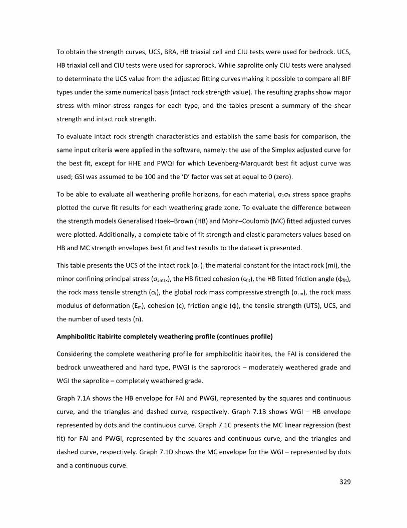
329
To obtain the strength curves, UCS, BRA, HB triaxial cell and CIU tests were used for bedrock. UCS,
HB triaxial cell and CIU tests were used for saprorock. While saprolite only CIU tests were analysed
to determinate the UCS value from the adjusted fitting curves making it possible to compare all BIF
types under the same numerical basis (intact rock strength value). The resulting graphs show major
stress with minor stress ranges for each type, and the tables present a summary of the shear
strength and intact rock strength.
To evaluate intact rock strength characteristics and establish the same basis for comparison, the
same input criteria were applied in the software, namely: the use of the Simplex adjusted curve for
the best fit, except for HHE and PWQI for which Levenberg-Marquardt best fit adjust curve was
used; GSI was assumed to be 100 and the ‘D’ factor was set at equal to 0 (zero).
To be able to evaluate all weathering profile horizons, for each material, σ1σ3 stress space graphs
plotted the curve fit results for each weathering grade zone. To evaluate the difference between
the strength models Generalised Hoek–Brown (HB) and Mohr–Coulomb (MC) fitted adjusted curves
were plotted. Additionally, a complete table of fit strength and elastic parameters values based on
HB and MC strength envelopes best fit and test results to the dataset is presented.
This table presents the UCS of the intact rock (σci), the material constant for the intact rock (mi), the
minor confining principal stress (σ3max), the HB fitted cohesion (cfit), the HB fitted friction angle (ɸfit),
the rock mass tensile strength (σt), the global rock mass compressive strength (σcm), the rock mass
modulus of deformation (Em), cohesion (c), friction angle (ɸ), the tensile strength (UTS), UCS, and
the number of used tests (n).
Amphibolitic itabirite completely weathering profile (continues profile)
Considering the complete weathering profile for amphibolitic itabirites, the FAI is considered the
bedrock unweathered and hard type, PWGI is the saprorock – moderately weathered grade and
WGI the saprolite – completely weathered grade.
Graph 7.1A shows the HB envelope for FAI and PWGI, represented by the squares and continuous
curve, and the triangles and dashed curve, respectively. Graph 7.1B shows WGI – HB envelope
represented by dots and the continuous curve. Graph 7.1C presents the MC linear regression (best
fit) for FAI and PWGI, represented by the squares and continuous curve, and the triangles and
dashed curve, respectively. Graph 7.1D shows the MC envelope for the WGI – represented by dots
and a continuous curve.
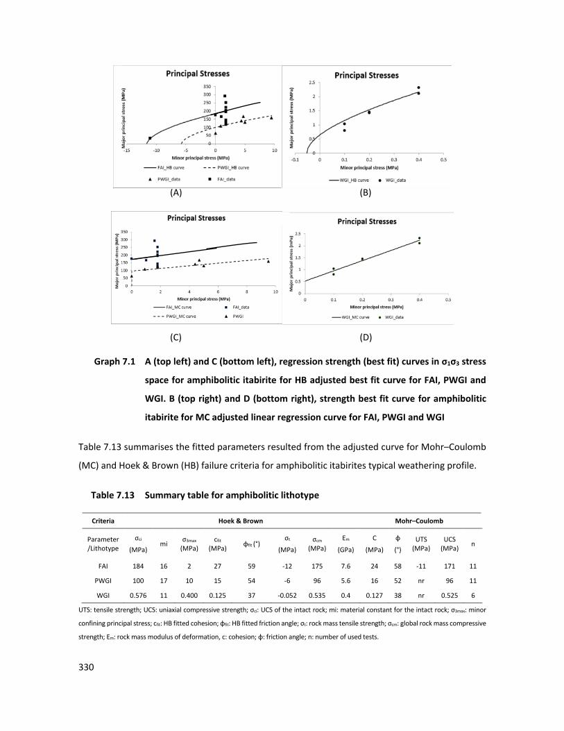
330
(A) (B)
(C) (D)
(C) (D)
0-1 Graph 7.1 A (top left) and C (bottom left), regression strength (best fit) curves in σ1σ3 stress
space for amphibolitic itabirite for HB adjusted best fit curve for FAI, PWGI and
WGI. B (top right) and D (bottom right), strength best fit curve for amphibolitic
itabirite for MC adjusted linear regression curve for FAI, PWGI and WGI
Table 7.13 summarises the fitted parameters resulted from the adjusted curve for Mohr–Coulomb
(MC) and Hoek & Brown (HB) failure criteria for amphibolitic itabirites typical weathering profile.
35 Table 7.13 Summary table for amphibolitic lithotype
Criteria Hoek & Brown Mohr–Coulomb
Parameter/Lithotype
σci
(MPa) mi σ3max
(MPa) cfit
(MPa) ɸfit (°) σt
(MPa) σcm
(MPa) Em
(GPa)
C
(MPa)
ɸ
(°) UTS
(MPa) UCS
(MPa) n
FAI 184 16 2 27 59 -12 175 7.6 24 58 -11 171 11
PWGI 100 17 10 15 54 -6 96 5.6 16 52 nr 96 11
WGI 0.576 11 0.400 0.125 37 -0.052 0.535 0.4 0.127 38 nr 0.525 6
UTS: tensile strength; UCS: uniaxial compressive strength; σci: UCS of the intact rock; mi: material constant for the intact rock; σ3max: minor
confining principal stress; cfit: HB fitted cohesion; ɸfit: HB fitted friction angle; σt: rock mass tensile strength; σcm: global rock mass compressive
strength; Em: rock mass modulus of deformation, c: cohesion; ɸ: friction angle; n: number of used tests.
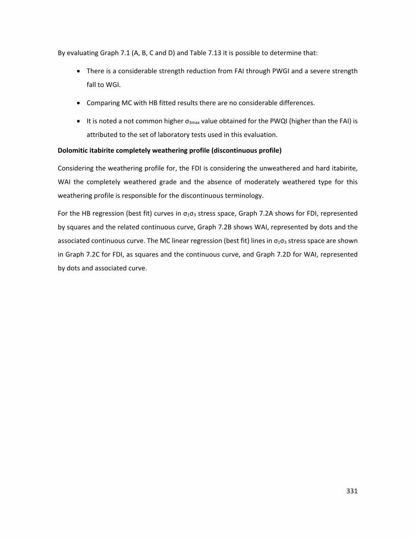
331
By evaluating Graph 7.1 (A, B, C and D) and Table 7.13 it is possible to determine that:
• There is a considerable strength reduction from FAI through PWGI and a severe strength
fall to WGI.
• Comparing MC with HB fitted results there are no considerable differences.
• It is noted a not common higher σ3max value obtained for the PWQI (higher than the FAI) is
attributed to the set of laboratory tests used in this evaluation.
Dolomitic itabirite completely weathering profile (discontinuous profile)
Considering the weathering profile for, the FDI is considering the unweathered and hard itabirite,
WAI the completely weathered grade and the absence of moderately weathered type for this
weathering profile is responsible for the discontinuous terminology.
For the HB regression (best fit) curves in σ1σ3 stress space, Graph 7.2A shows for FDI, represented
by squares and the related continuous curve, Graph 7.2B shows WAI, represented by dots and the
associated continuous curve. The MC linear regression (best fit) lines in σ1σ3 stress space are shown
in Graph 7.2C for FDI, as squares and the continuous curve, and Graph 7.2D for WAI, represented
by dots and associated curve.
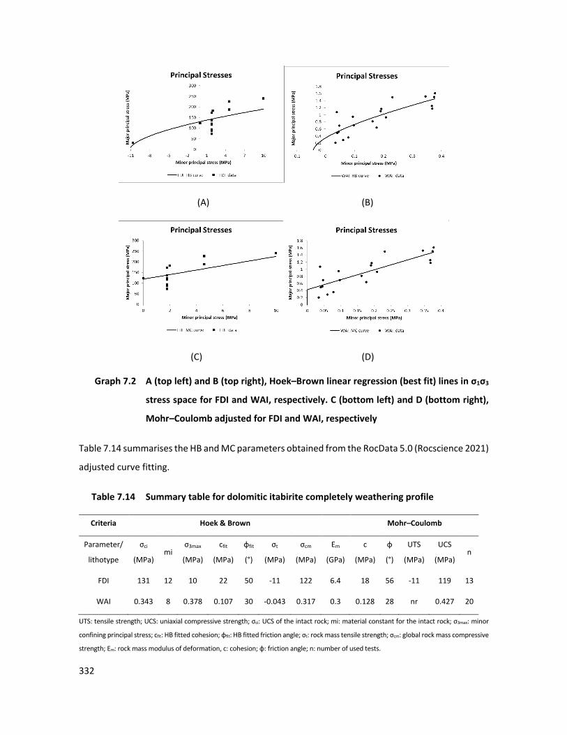
332
(A) (B)
(C) (D)
0-2 Graph 7.2 A (top left) and B (top right), Hoek–Brown linear regression (best fit) lines in σ1σ3
stress space for FDI and WAI, respectively. C (bottom left) and D (bottom right),
Mohr–Coulomb adjusted for FDI and WAI, respectively
Table 7.14 summarises the HB and MC parameters obtained from the RocData 5.0 (Rocscience 2021)
adjusted curve fitting.
36 Table 7.14 Summary table for dolomitic itabirite completely weathering profile
Criteria Hoek & Brown Mohr–Coulomb
Parameter/
lithotype
σci
(MPa) mi
σ3max
(MPa)
cfit
(MPa)
ɸfit
(°)
σt
(MPa)
σcm
(MPa)
Em
(GPa)
c
(MPa)
ɸ
(°)
UTS
(MPa)
UCS
(MPa) n
FDI 131 12 10 22 50 -11 122 6.4 18 56 -11 119 13
WAI 0.343 8 0.378 0.107 30 -0.043 0.317 0.3 0.128 28 nr 0.427 20
UTS: tensile strength; UCS: uniaxial compressive strength; σci: UCS of the intact rock; mi: material constant for the intact rock; σ3max: minor
confining principal stress; cfit: HB fitted cohesion; ɸfit: HB fitted friction angle; σt: rock mass tensile strength; σcm: global rock mass compressive
strength; Em: rock mass modulus of deformation, c: cohesion; ɸ: friction angle; n: number of used tests.
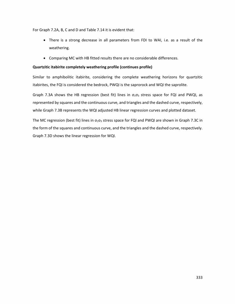
333
For Graph 7.2A, B, C and D and Table 7.14 it is evident that:
• There is a strong decrease in all parameters from FDI to WAI, i.e. as a result of the
weathering.
• Comparing MC with HB fitted results there are no considerable differences.
Quartzitic itabirite completely weathering profile (continues profile)
Similar to amphibolitic itabirite, considering the complete weathering horizons for quartzitic
itabirites, the FQI is considered the bedrock, PWQI is the saprorock and WQI the saprolite.
Graph 7.3A shows the HB regression (best fit) lines in σ1σ3 stress space for FQI and PWQI, as
represented by squares and the continuous curve, and triangles and the dashed curve, respectively,
while Graph 7.3B represents the WQI adjusted HB linear regression curves and plotted dataset.
The MC regression (best fit) lines in σ1σ3 stress space for FQI and PWQI are shown in Graph 7.3C in
the form of the squares and continuous curve, and the triangles and the dashed curve, respectively.
Graph 7.3D shows the linear regression for WQI.
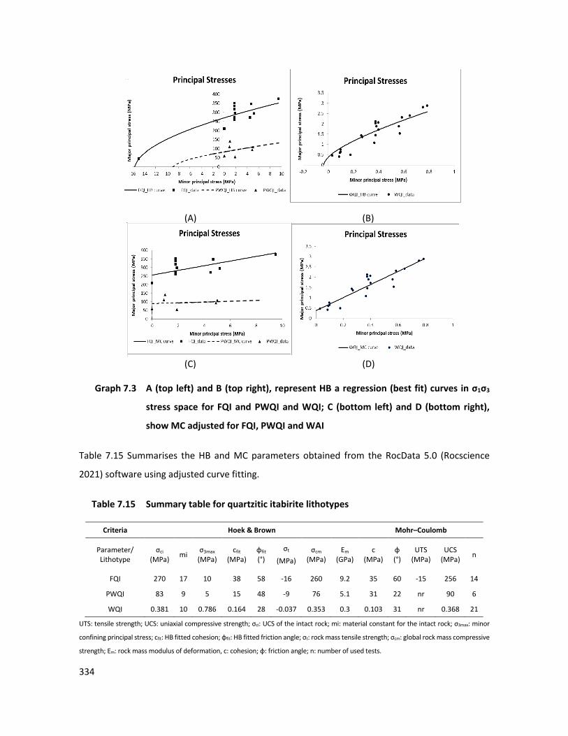
334
(A) (B)
(C) (D)
0-3 Graph 7.3 A (top left) and B (top right), represent HB a regression (best fit) curves in σ1σ3
stress space for FQI and PWQI and WQI; C (bottom left) and D (bottom right),
show MC adjusted for FQI, PWQI and WAI
Table 7.15 Summarises the HB and MC parameters obtained from the RocData 5.0 (Rocscience
2021) software using adjusted curve fitting.
37 Table 7.15 Summary table for quartzitic itabirite lithotypes
Criteria Hoek & Brown Mohr–Coulomb
Parameter/ Lithotype
σci
(MPa) mi σ3max
(MPa) cfit
(MPa) ɸfit
(°) σt
(MPa) σcm
(MPa) Em
(GPa) c
(MPa) ɸ (°)
UTS (MPa)
UCS (MPa) n
FQI 270 17 10 38 58 -16 260 9.2 35 60 -15 256 14
PWQI 83 9 5 15 48 -9 76 5.1 31 22 nr 90 6
WQI 0.381 10 0.786 0.164 28 -0.037 0.353 0.3 0.103 31 nr 0.368 21
UTS: tensile strength; UCS: uniaxial compressive strength; σci: UCS of the intact rock; mi: material constant for the intact rock; σ3max: minor
confining principal stress; cfit: HB fitted cohesion; ɸfit: HB fitted friction angle; σt: rock mass tensile strength; σcm: global rock mass compressive
strength; Em: rock mass modulus of deformation, c: cohesion; ɸ: friction angle; n: number of used tests.
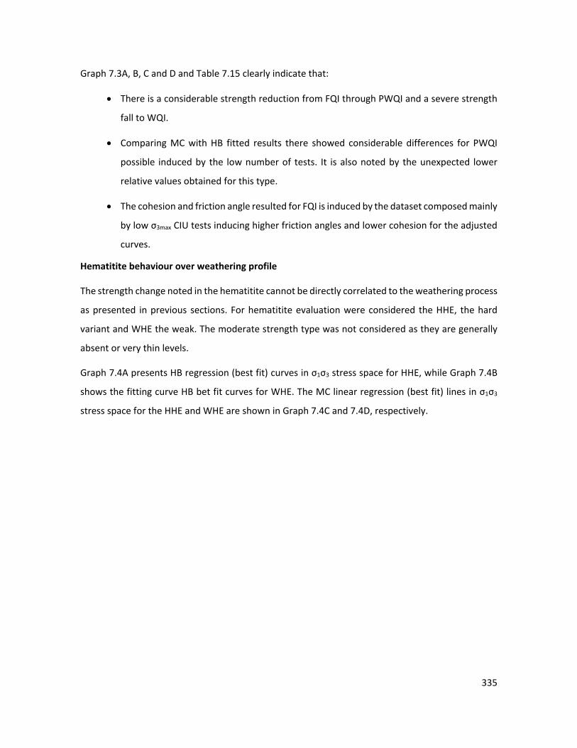
335
Graph 7.3A, B, C and D and Table 7.15 clearly indicate that:
• There is a considerable strength reduction from FQI through PWQI and a severe strength
fall to WQI.
• Comparing MC with HB fitted results there showed considerable differences for PWQI
possible induced by the low number of tests. It is also noted by the unexpected lower
relative values obtained for this type.
• The cohesion and friction angle resulted for FQI is induced by the dataset composed mainly
by low σ3max CIU tests inducing higher friction angles and lower cohesion for the adjusted
curves.
Hematitite behaviour over weathering profile
The strength change noted in the hematitite cannot be directly correlated to the weathering process
as presented in previous sections. For hematitite evaluation were considered the HHE, the hard
variant and WHE the weak. The moderate strength type was not considered as they are generally
absent or very thin levels.
Graph 7.4A presents HB regression (best fit) curves in σ1σ3 stress space for HHE, while Graph 7.4B
shows the fitting curve HB bet fit curves for WHE. The MC linear regression (best fit) lines in σ1σ3
stress space for the HHE and WHE are shown in Graph 7.4C and 7.4D, respectively.
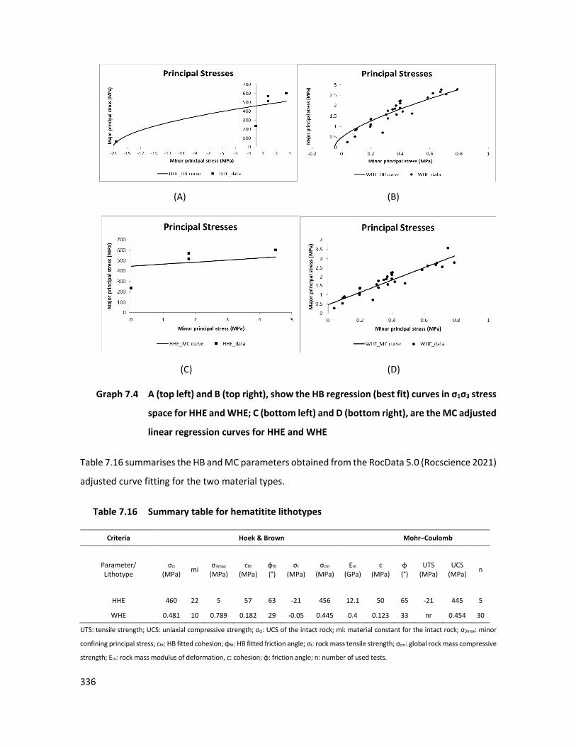
336
(A) (B)
(C) (D)
0-4 Graph 7.4 A (top left) and B (top right), show the HB regression (best fit) curves in σ1σ3 stress
space for HHE and WHE; C (bottom left) and D (bottom right), are the MC adjusted
linear regression curves for HHE and WHE
Table 7.16 summarises the HB and MC parameters obtained from the RocData 5.0 (Rocscience 2021)
adjusted curve fitting for the two material types.
38 Table 7.16 Summary table for hematitite lithotypes
Criteria Hoek & Brown Mohr–Coulomb
Parameter/ Lithotype
σci
(MPa) mi σ3max
(MPa) cfit
(MPa) ɸfit
(°) σt
(MPa) σcm
(MPa) Em
(GPa) c
(MPa) ɸ (°)
UTS (MPa)
UCS (MPa) n
HHE 460 22 5 57 63 -21 456 12.1 50 65 -21 445 5
WHE 0.481 10 0.789 0.182 29 -0.05 0.445 0.4 0.123 33 nr 0.454 30
UTS: tensile strength; UCS: uniaxial compressive strength; σci: UCS of the intact rock; mi: material constant for the intact rock; σ3max: minor
confining principal stress; cfit: HB fitted cohesion; ɸfit: HB fitted friction angle; σt: rock mass tensile strength; σcm: global rock mass compressive
strength; Em: rock mass modulus of deformation, c: cohesion; ɸ: friction angle; n: number of used tests.
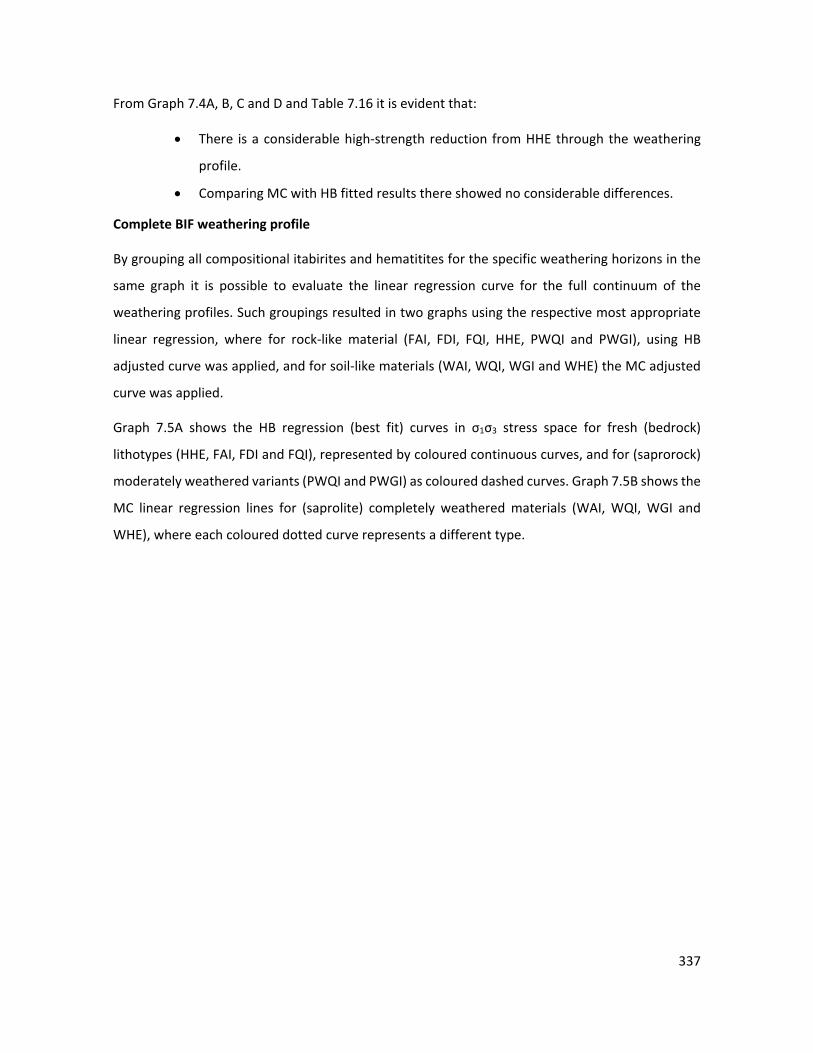
337
From Graph 7.4A, B, C and D and Table 7.16 it is evident that:
• There is a considerable high-strength reduction from HHE through the weathering
profile.
• Comparing MC with HB fitted results there showed no considerable differences.
Complete BIF weathering profile
By grouping all compositional itabirites and hematitites for the specific weathering horizons in the
same graph it is possible to evaluate the linear regression curve for the full continuum of the
weathering profiles. Such groupings resulted in two graphs using the respective most appropriate
linear regression, where for rock-like material (FAI, FDI, FQI, HHE, PWQI and PWGI), using HB
adjusted curve was applied, and for soil-like materials (WAI, WQI, WGI and WHE) the MC adjusted
curve was applied.
Graph 7.5A shows the HB regression (best fit) curves in σ1σ3 stress space for fresh (bedrock)
lithotypes (HHE, FAI, FDI and FQI), represented by coloured continuous curves, and for (saprorock)
moderately weathered variants (PWQI and PWGI) as coloured dashed curves. Graph 7.5B shows the
MC linear regression lines for (saprolite) completely weathered materials (WAI, WQI, WGI and
WHE), where each coloured dotted curve represents a different type.
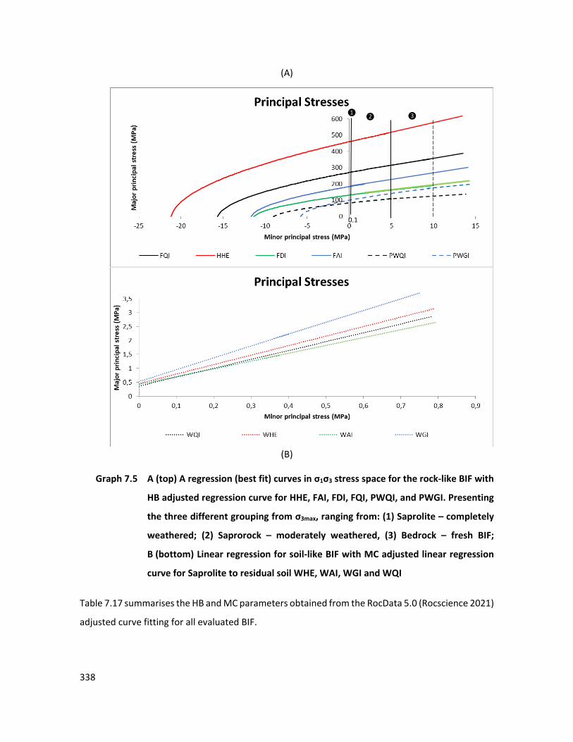
338
(A)
(B)
0-5 Graph 7.5 A (top) A regression (best fit) curves in σ1σ3 stress space for the rock-like BIF with
HB adjusted regression curve for HHE, FAI, FDI, FQI, PWQI, and PWGI. Presenting
the three different grouping from σ3max, ranging from: (1) Saprolite – completely
weathered; (2) Saprorock – moderately weathered, (3) Bedrock – fresh BIF;
B (bottom) Linear regression for soil-like BIF with MC adjusted linear regression
curve for Saprolite to residual soil WHE, WAI, WGI and WQI
Table 7.17 summarises the HB and MC parameters obtained from the RocData 5.0 (Rocscience 2021)
adjusted curve fitting for all evaluated BIF.
0.1 0.1
❶ ❷ ❸
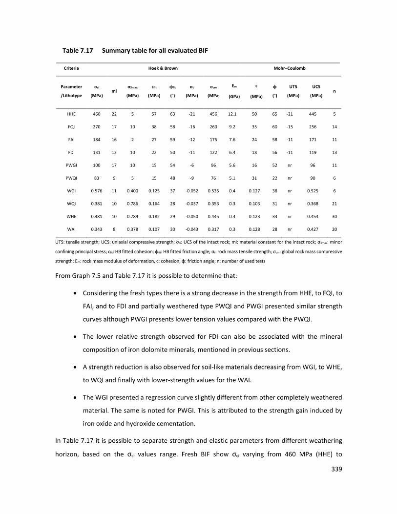
339
39Table 7.17 Summary table for all evaluated BIF
Criteria Hoek & Brown Mohr–Coulomb
Parameter
/Lithotype
σci
(MPa) mi
σ3max
(MPa)
cfit
(MPa)
ɸfit
(°)
σt
(MPa)
σcm
(MPa)
Em
(GPa)
c
(MPa)
ɸ
(°)
UTS
(MPa)
UCS
(MPa) n
HHE 460 22 5 57 63 -21 456 12.1 50 65 -21 445 5
FQI 270 17 10 38 58 -16 260 9.2 35 60 -15 256 14
FAI 184 16 2 27 59 -12 175 7.6 24 58 -11 171 11
FDI 131 12 10 22 50 -11 122 6.4 18 56 -11 119 13
PWGI 100 17 10 15 54 -6 96 5.6 16 52 nr 96 11
PWQI 83 9 5 15 48 -9 76 5.1 31 22 nr 90 6
WGI 0.576 11 0.400 0.125 37 -0.052 0.535 0.4 0.127 38 nr 0.525 6
WQI 0.381 10 0.786 0.164 28 -0.037 0.353 0.3 0.103 31 nr 0.368 21
WHE 0.481 10 0.789 0.182 29 -0.050 0.445 0.4 0.123 33 nr 0.454 30
WAI 0.343 8 0.378 0.107 30 -0.043 0.317 0.3 0.128 28 nr 0.427 20
UTS: tensile strength; UCS: uniaxial compressive strength; σci: UCS of the intact rock; mi: material constant for the intact rock; σ3max: minor
confining principal stress; cfit: HB fitted cohesion; ɸfit: HB fitted friction angle; σt: rock mass tensile strength; σcm: global rock mass compressive
strength; Em: rock mass modulus of deformation, c: cohesion; ɸ: friction angle; n: number of used tests
From Graph 7.5 and Table 7.17 it is possible to determine that:
• Considering the fresh types there is a strong decrease in the strength from HHE, to FQI, to
FAI, and to FDI and partially weathered type PWQI and PWGI presented similar strength
curves although PWGI presents lower tension values compared with the PWQI.
• The lower relative strength observed for FDI can also be associated with the mineral
composition of iron dolomite minerals, mentioned in previous sections.
• A strength reduction is also observed for soil-like materials decreasing from WGI, to WHE,
to WQI and finally with lower-strength values for the WAI.
• The WGI presented a regression curve slightly different from other completely weathered
material. The same is noted for PWGI. This is attributed to the strength gain induced by
iron oxide and hydroxide cementation.
In Table 7.17 it is possible to separate strength and elastic parameters from different weathering
horizon, based on the σci values range. Fresh BIF show σci varying from 460 MPa (HHE) to
340
131 MPa (FDI). Moderately weathered BIF show σci varying from 100 MPa (PWGI) to 80 MPa (PWQI).
Completely weathered BIF show σci varying from 0.576 MPa (WGI) to 0.343 MPa (WAI).
Based on Graph 7.5, three groups separated by the σ3max were determined:
• BIF saprolite horizon: Completely weathered BIF, from 0.789 MPa for the WGI to 0.378 MPa
for WAI with a σ3max ≤ 1 MPa;
• BIF saprorock horizon: Moderately weathered BIF, from 10 MPa for the PWGI to 5 MPa for
PWQI with a σ3max raging 1 MPa < σ3max ≤ 5 MPa;
• BIF bedrock horizon: Fresh BIF, from 10 MPa for the FQI to 2 MPa for FAI σ3max > 5 MPa.
7.6 DISCUSSION
Anisotropy and heterogeneity from BIF weathering profiles
The itabirite compositional metamorphic banding is defined by the alteration of iron and non-iron
bands forms the itabirite heterogeneity, which is promoted by its bimodal mineral composition,
mineral hardness, bulk density, fabric, and total porosity, and are controlled by the associated
degree of weathering and iron content. The hematitite metamorphic banding is defined by the
alternation of different iron minerals, total porosity, and fabric, defining a hematitite heterogeneity.
Contact surfaces between heterogeneity of itabirites (iron and non-iron bands) and hematitites
(higher total porosity and lower total porosity bands) define porous layers and mineral orientation.
These weaker surfaces are potentially prone to driving the weathering and to generating individual
discontinuity planes (e.g. ubiquitous joints), or to inducing an increase in the anisotropy ratio for
more weathered BIF. Depending on the weathering horizon and zone, these possible contact planes
generally represent single discontinuities not penetrative for fresh to slightly weathered BIF. They
can also generate penetrative and persistent surfaces that will induce medium anisotropy ratios in
FDI, PWQI and PWGI.
Given the several uncertainties about their geneses, it is possible to assert that hematitite and
itabirite groups present significantly different behaviours, even with similar intact rock strength. It
can be argued that the itabirite group behaviour is primarily induced by mineral composition
(heterogeneity) and secondarily by the total porosity. For this rock the intact strength, and
heterogeneity are highly influenced by the geological and structural settings of the original bedrock.
341
The bedrock with typical compositional metamorphic banding, was progressively transformed by
the iron enrichment process and weathering in the different BIF types through moderately
weathered variants to residual soils, resulting in a complex tridimensional weathering profile with
not only vertical but also lateral variation. The profile variations result from the banding, structures
and weathering interaction, defining at least two different types of weathering profiles associated
with the proto-ore mineralogical composition, namely, a discontinuous weathering profile for easily
leached BIF lithology such as FDI, and the continuous weathering profile for other BIF less prone to
leaching, e.g. FAI and FQI.
Such complex variations result in different weathering profile characteristics. When considering
each compositional itabirite, the dolomitic proto-ore (FDI) shows the deepest weathering profiles
taking into consideration the saprolite horizon thickness. At the Águas Claras, Mutuca and Capão
Xavier mines saprolite can easily reach 400 m in depth with completely weathered BIF (WHE and
WAI) showing no transitional (saprorock – moderately weathered) material. For quartzitic proto-ore
(FAI and FQI) the weathering profile is also as deep, as observed at the Tamanduá, Capitão do Mato,
Pico and other mines, where it is defined by a sequential weathering range from fresh to residual
soil in which the thickness of the transitional saprorock (PWQI and PWGI) can vary from tens to
hundreds of metres, depending on intrinsic and extrinsic characteristics as originally proposed by
Dorr (1969).
The iron enrichment based on supergenic or hypogenic genesis, and metamorphic and tectonic
setting, should affect hematitite (hard or weak) total porosity and fabric, (i.e. mineral and pores size,
and orientation), establishing the different levels of intact rock strength consistency and hardness
that could not be divided and associated to the weathering horizons. In these materials, the typical
compositional metamorphic banding and hypogene enrichment for HHE and supergene enrichment
for WHE are the main process and weathering plays a secondary role, being responsible for
hematitite oxidation and secondary total porosity increase mainly for the completely weathered
grades. The weak hematitite genesis is controversial and is a result from hypogene and supergene
process defined by Ramanaidou & Morris (2010) as supergenic mimetic mechanism from previous
itabirites.
Additionally, as in great depths the iron enrichment process were not efficient for itabirites, the
total porosity for fresh BIF is originally imposed by the low-grade regional metamorphism imposing
a granuloblast texture, with small crystals oriented according to a banding. At shallower depths,
342
supergene events transformed the crystalline phases of iron minerals (hematite, magnetite and
martite), providing a volumetric reduction which is responsible for increased intergranular porosity
(Pimenta 1992). Finally, the lattice weathering process induce oxidation and other mineral changes
(deleterious minerals) responsible to increase the total porosity and reduce the intact rock strength.
These considerations agree with studies by Rosière et al. (1993), Lagoeiro (1998), Morris (2002 and
2002a) and Costa et al. (2009) which suggest that the origin of high-strength, hard hematite is
associated with original band concentration during depositional events by hypogenic fluids that
were concentrated in fold axes, interception of foliations or banding, and/or near intrusive dikes.
These studies also indicate that at close to the surface, low strength hematitites (brown hematite)
is associated with an ancient supergene origin (mimetic weathering), mainly by the surface
weathering in itabirites.
From the weathering, for the hematitite group it is recognised that increases in total porosity and
mineral alteration are important changes that produce an effective softening of the original fresh
rocks.
For itabirites, this softening is produced by partial or total leaching of non-iron minerals, mainly iron
dolomite, but also quartz; oxidation of iron minerals; and chemical alteration of amphibole and
other minerals. In extreme cases, the remaining iron oxidises, and non-iron bands (mainly quartz)
exhibit a high total porosity and low grain apparent cohesion (loss of contact between grains). This
results in a weak material that is occasionally cemented by secondary iron oxides and/or hydroxides
(WGI and PWGI), which impose some additional strength due to the total porosity reduction. These
results outlined above agree with studies by Gupta & Rao (2001) for crystalline rocks, Marques et
al. (2010) for metamorphic rocks and Leão et al. (2017) for phyllites.
Weathering changes imposed on BIF through the weathering profiles
Supporting geological and geotechnical considerations, laboratory tests undertaken especially for
these studies and results from Vale’s database show a significant reduction of intact rock strength
and elastic parameters from fresh to completely weathered BIF types. These changes are presented
and described below, for each weathering horizon:
• Fresh to slightly weathered (bedrock horizon)
343
At great depths, for this horizon, even with a reduced opening of pre-existent fractures promotes
some initial oxidation at discontinuities walls. Additionally, weathering of the band boundaries with
higher pore levels could increase the oxidation also defining slightly weathered types (W2).
At this stage, intact rock strength reduction is very low, and the real changes are observed only in
the strength reductions on discontinuities walls for fresh BIF and the typical compositional
metamorphic banding is preserved. The anisotropy is insipient induced by the heterogeneity for
itabirites and pores layers for HHE.
The intact rock strengths for fresh and hard BIF show a progressive reduction from HHE, through
FQI and FAI to FDI. The lower values seen for FDI is attributed to the presence of weaker minerals
(e.g. siderite and ankerite), and fabric with higher relative grain size variation associated with
weaker banding planes at the contact between iron dolomitic and iron bands. This characteristic is
also responsible for inducing a low to medium anisotropic ratio for FDI (Rc = 2).
Conversely, the higher intact rock strength of HHE is induced by the mono-mineral composition,
with denser and harder iron minerals that induce a higher bulk density and higher intact rock
strength, and an anisotropy ratio of Rc = 1 defined as isotropic.
However, considering anisotropic effects for HHE, the obtained values presented some
inconsistencies mainly due to the low number of test results obtained for β90° due to the difficulty
in extracting reliable samples, which could have induced some bias.
The HHE must be treated separately since they are mainly a product of hypogenic enrichment, for
this reason are not directly associated with the weathering grade continuum.
• Moderately weathered (saprorock horizons)
For this horizon, in the first few hundred metres below the surface, the intense strength reduction
is not restricted to fractures but is also related to the intact rock developing through band contacts
and higher total porous layers increasing the total porosity by leaching of non-iron bands and
oxidation of iron bands in these zones.
In this horizon, the metamorphic banding orientation competes with the new forming weathering
banding that could or not be parallel one with other depending on the topography and metamorphic
banding dip.
344
For FDI, the typical discontinuous weathering profile does not present saprorock horizons. The
supergene alteration occurs in a single stage, inducing a complete leaching of the iron dolomite
minerals and loss of grain cohesion for all bands, thereby resulting in a total change from FDI
to WHE or WAI, depending on geological settings as described by Spier et al. (2008).
Due to the lower solubility of quartz in FQI and FAI, the supergene process is less effective and the
moderately weathered types (PWQI and PWGI) are present, defining a thicker saprorock horizon
ranging from tens of meters to several hundred of meters, normally observed in continuous
weathering profile.
Anisotropic effects are induced in this stage by the intact rock strength reduction and higher number
of open discontinuities, increasing of the total porosity as a result of partial or total leaching, and
iron mineral alteration inducing a loss of apparent grain cohesion, mainly in the quartz bands but
also in iron bands reflecting a medium anisotropy degree (Rc = 2.6) and resulting in a clear
heterogeneity observed in these types.
For moderately weathered itabirites, the σci for PWGI is higher than for PWQI, even with the reduced
number of tests, anisotropic grouping indicates a sensitive reduction of elastic and intact rock
strength parameters at β45°.
• Completely weathered to residual soil (saprolite to residual soil horizons)
At shallower depths to the surface, these horizons present respectively weak rock and soil material
resulted from a total softening, loss of grain cohesion and an increase of total porosity for all bands,
resulting in an accentuated strength reduction. Deep oxidation and hydration of iron minerals are
abundant for the residual soil horizon but are not necessarily found at saprolite horizon.
For BIF saprolite horizon, the anisotropy for WAI, displays a low anisotropy ratio associated with the
presence of clay bands. These bands display very low shear strength levels when compared with
quartz or hematite bands.
WGI is geologically similar to WQI, with the main difference being related to the greater presence
of goethite as cement that increases the weathering degree, but conversely also increases the shear
rock strength due to the porous cementation. For this reason, WGI presents higher intact rock
strength values.
345
WQI, with the quartz partial leaching and iron enrichment induces a ρb increase even with total
porosity increase. For the WHE, contrarily, a total leaching of non-iron bands will induce an increase
in the ρb as all the soil is constituted mainly of denser minerals (hematite and martite) even with
high total porosity. Consequentially, the WHE strength is higher at saprolite horizon.
Specially for shallower depths, where all geological processes are more effective, the balance
between intrinsic characteristics such as iron content, total porosity, bulk density, iron cementation
and shear strength, and extrinsic characteristics such as porewater content define a multivariable
correlation difficult to track that controls the BIF weak rock behaviour. This process is presented by
Ramanaidou & Morris (2010), who argue that weathering softening is primarily due to the
dissolution and reprecipitation defined by supergene mimetic iron enrichment, and secondly the
result of the supergene laterite fluids that are mainly responsible for the oxidation of iron minerals:
in other words, ‘weathering’. It was also evaluated, considering the supergene alteration process
that induces sufficient porosity increases to generate subsidence, as proposed by Ribeiro & Carvalho
(2002) and Ribeiro (2003).
Failure criteria through the BIF weathering profile
• MC and HB failure criteria are widely applied to define intact rock strength parameters for
iron ore mines. Each one has been used and defined as more appropriated for evaluate
rock (HB) and soil or soil-like (MC) materials. For isotropic to low anisotropy fresh/hard
lithologies showed HB regression curves with a progressive strength reduction from HHE,
FQI, to FAI, presenting similar curves, indicating that these lithologies display similar
strength behaviour.
• For low to medium anisotropy FDI and PWQI showed lower HB strength curves and PWGI
a particularly distinct envelope, indicating higher strength attributed to a strength increase
resulting from the presence of iron oxide cement.
• For highly to completely weathered BIF, the use of MC criterion indicates a similar friction
angle for all types except for the WGI with the highest value, attributed to the presence of
iron oxide and hydroxy such as cement and WAI with lower MC curve promoted by the
presence of clay minerals that will finally affect the porewater pressure for unsaturated
condition.
346
7.7 CONCLUSION
The use of geological and geotechnical criteria allows the elimination of atypical BIF features, and
simple statistical approaches were used to define outliers, these approaches emphasising the
importance of data evaluation to provide best fit results, reducing the natural variance observed at
laboratory test results.
The itabirite compositional metamorphic banding defined by the iron and non-iron band alternation
which configure the itabirite heterogeneity is promoted by bimodal mineral composition, mineral
fabric, bulk density, mineral hardness, and total porosity, that are primary imposed by the
metamorphic grade (greater depths), supergene events, all of which are controlled by the
weathering degree and banding thickness.
For itabirites, intact rock strength and elastic parameter are associated with the weathering horizon
and zones and present similar parameters associated with the itabirite composition grouping, e.g.
quartz-based types (quartzitic, amphibolitic) and iron dolomite-based type (FDI). The hematitic
group, although having different genesis and must considerate with restrictions as a part of the
weathering profile. Among other critical characteristic presents in general higher bulk density and
intact rock strength compared with other itabirites.
The hematitite metamorphic banding is defined by alteration of different iron minerals and total
porosity, and also in texture, and shape at all weathering horizons. Thereby defining a hematitite
heterogeneity that are primarily imposed by the metamorphic grade and hypogene process for HHE,
and metamorphic grade and supergene process for WHE (mimetic supergene enrichment,
Ramanaidou 1989 and 2009), all of which are not (or partially) controlled by the weathering degree.
For the hematitite, tectonic and/or metamorphic conditions are the main factors controlling intact
rock strength reduction. Weathering (laterite weathering enrichment, Ramanaidou 1989 and 2009)
has only a secondary effect on intact rock strength variations of this type by iron oxidation reducing
the strength along bad planes or discontinuities.
At bedrock horizon in great depths, the anisotropy effect is attributed to the compositional
metamorphic banding in typical itabirite heterogeneities, are promoted by minerology. For this
reason, the mineralogical composition is more effective in lithotypes with higher mineral hardness
contrasts, as noted in the FDI, due to the high contrast between iron bands (hematite and martite),
with non-iron bands (ankerite and siderite). Total porosity can cause minor anisotropy effects in
347
intact rock strengths for fresh weathering degree but is mandatory to increase the anisotropy for
PWQI/PWGI which show medium anisotropy ratios.
UCS, triaxial HB and Brazilian test data analysed with RocData 5.0 (Rocscience 2021) provides
reliable linear regression (best fit) lines in σ1σ3 stress space, which were used to determine intact
rock strengths and static elastic parameters for different weathered levels. Mohr–Coulomb and
Hoek–Brown criteria were evaluated and compared for all materials, resulting in similar adjusted
parameters.
From the fifteen mines that were studied, two different types of weathering profile were identified.
The discontinuous profile presents no saprorock with moderately weathered materials (W3 and
W4), between the hard and fresh bedrock horizon to weak and highly weathered saprolite horizon,
indicating a discontinuous weathering profile. This type is observed at the Águas Claras, Mutuca and
Capão Xavier mines, where the high leaching-prone proto-ore is mainly composed of dolomitic
itabirites. These profiles present the deeper saprolites horizon level, reaching over 400 m in depth.
The second type includes a transition zone, forming a continuous weathering profile, in which
saprorock (moderately weathered types) can vary in thickness from tens to hundreds of metres.
This profile is generally observed in mines where the proto-ore is less prone to leaching, composed
of amphibolitic and/or quartzitic itabirites, such as in the Tamanduá, Capitão do Mato, and Pico
Mines.
Each profile type is defined by the weathering horizons and zones, and the tridimensional spatial
distribution is highly conditioned by the itabirite compositional metamorphic banding geological
setting (folds and faults), depth, topography and other external characteristics as e.g. pluviometry
and temperature.
Considering these different weathering profiles for itabirite it is possible to group and summarise
the main characteristics:
• Bedrock: fresh itabirites (FDI, FQI and FAI) generally display low values of total porosity
(5% to 10%) and a medium ρb (3.11 t/m3 to 3.41 t/m3). These characteristics are supported
by the basic mineralogy (iron dolomite, quartz, and hematite), and the mineral shapes
(tabular to granoblastic). UCS values range from quartzitic itabirite (UCSFQI = 256 MPa) and
amphibolitic itabirite (UCS FAI = 171 MPa) to the lowest dolomitic itabirite
(UCSFDI = 119 MPa) but with a higher anisotropy rate. Due to the differences in geological
348
genesis, the stronger hematitite (UCSHHE = 445 MPa) must be considered in a different
group.
• Moderately weathered itabirites at saprorock horizon (PWQI and PWGI), have
intermediate total porosity (10% to 20%), high ρb (3.6 t/m3 to 3.26 t/m3) and considerably
lower UCS values (UCSPWQI/PWGI = 68 MPa). This high strength reduction is associated with
the increase in anisotropy ratio and total porosity.
• Highly to completely weathered itabirite at saprolite and residual soil horizons present
very high porosity (20% to 30%) and very low bulk density varying from ρb (2.2 t/m3
to 2.7 t/m3) present very low relative UCS values, decreasing from the strongest WGI
(UCSWGI = 0.53 MPa) to moderately weak hematitite (UCSWHE = 0.45 MPa) and argillaceous
itabirite (UCSWAI = 0.37 MPa) and to a lower mean for the WQI (UCSWQI = 0.37 MPa).
• The iron enrichment process, in this stage will produce two different types of saprolite
materials: itabiritic (WQI, WGI and WAI), with the partial leaching inducing a bulk density
and total porosity decrease. For hematitic (WHE), the total leaching (supergenic iron
enrichment) of non-iron minerals induced a higher bulk density (ρb = 3.5t/m3) even
increasing the total porosity. Consequentially, the WHE shear strength is higher than WQI
due to the iron content.
In summary, for BIFs:
• The metamorphic grade and tectonical settings, are responsible for the mineral
composition and fabric are responsible for the original mineral hardness, grain contacts
and mineral orientation (size, shape, and texture) mainly at great depths for bedrock.
• In shallower depths, supergenic and hypogenic iron enrichment processes are responsible
for modifying the original configuration, reducing, or increasing intact rock strength
depending on the lithotype, and inducing iron concentration and ρb increases mainly for
hematitites, but also for rich itabirite lithotypes.
• At sallower depths to surface, the weathering grade increase (mainly total porosity
increase) is responsible for inducing medium anisotropy in PWQI and PWG.
• Mineral composition is responsible for inducing anisotropy for FDI.
349
• Since the bulk density is an important parameter responsible for the intact rock strength
behaviour, it is crucial to understand the balance between iron content and the total
porosity through the weathering profile to appreciate the intact rock strength behaviour
of the BIF. Additionally, these characteristics are highly affected by the mineral
composition and band thickness that could induce scale effect in tested samples.
• The evaluations of visual total porosity from thin sections demonstrate a direct increase
as the weathering grade increases. The Øb increment noted in evaluated thin sections
varies from one to four times for fresh to completely weathered BIF.
• Based on the UCS values obtained from HB failure envelopes, strength reductions of 55%
from fresh to moderately weathered, and of 48% from moderately to completely
weathered BIF were noted, illustrating an effective strength softening due to the
weathering.
• Moderately weathered lithotypes are important due to the ambiguous behaviours
observed at saprorock horizon typifying the boundary between fresh (bedrock, controlled
by typical compositional metamorphic banding) and completely weathered BIF (saprolite,
controlled by a mixture of metamorphic banding, supergene and weathering processes).
Such intermediate materials can behave like rock, when the leaching process was not
sufficiently effective to increase total porosity and when iron remobilisation fills the
porosity induced by the weathering at saprorock horizon increasing the intact rock
strength, or like a soil when the iron remobilisation only partially seals the pores leaving,
highly porous zones at saprolite horizon.

350
351
CHAPTER 8. CONCLUDING REMARKS
The research objectives of this thesis were presented and discussed in Chapters 1.2 to 1.4 and the
main findings and their respective contributions are summarised and divided based on the three
following distinct groups of materials, namely:
• Fresh to moderately weathered BIF types and their geological, petrophysical, intact rock
strength and elastic parameters, in association with the geomechanical behaviour
considering the anisotropy and heterogeneity characteristics. These results are presented
and discussed in Chapters 4 and 5, and Appendix I.
• The completely weathered to residual soils BIF types and their geological, petrophysical,
saturated and unsaturated shear strength and elastic parameters, in association with the
geomechanical behaviour considering the anisotropy and heterogeneity characteristics.
These results are presented and discussed in Chapter 6 and Appendix II.
• BIF completely weathered profile geological and geomechanical characteristics,
considering the weathering horizons and zones boundaries, and heterogeneities;
presented mainly in Chapter 7.
A summary of the conclusions along with a critical insight into the current and future work is
demonstrated in the following sections.
8.1 FRESH TO MODERATELY WEATHERED BIF GEOLOGICAL AND GEOMECHANICAL
CHARACTERISATION
Related to the variation obtained in the used dataset for rock materials definitions. In this thesis,
some laboratory test results presented high amplitude (standard deviation), indicating the presence
of a natural variance related to anisotropy, randomness of geological features and scale effect
related to the banding thickness and the sample size. Part of this behaviour is attributed to the
presence of low anisotropy effect and the samples natural heterogeneity even when adopting
coherent groupings and methodologies to eliminate outliers and reduce the natural variation and
others experimental problems presented above. Likewise, the tested materials present geological
features responsible for inducing large dispersions of the results, since they may have different
variations in fabric, rock heterogeneity and band thickness. In this matter, BIF was considered in this
thesis as a typical geological feature of the homogeneous sub centimetric parallel banding. Other
352
geological features considered not typical, e.g. intense fold, shear or breeched zones or veins must
be avoided from tested samples.
The field survey provided geological and geotechnical characterisation useful to group and remove
non-suitable laboratory test results from the dataset reducing bias and data variance. This approach
emphasised the role of identifying the geological characteristics that were crucial to define a proper
sample grouping, i.e. to separate the hematitite from itabirite group and better represent mainly
the three different compositional types of fresh itabirites. Based on laboratory tests, it was possible
to evaluate the intact rock strength and its static and dynamic elastic parameters. Thin sections
added important information to explain and show for each rock the fabric behaviour, visual
qualitative total porosity and correlation with results from laboratory tests.
Even with several attempts to reduce data dispersion, some parameters still showed high standard
deviation. This may represent a natural range expected for these properties and/or by the slightly
higher anisotropic ratio (medium anisotropy) observed for FDI, PWQI and PWGI. Even so, it was
possible to verify reliable trends and establish proper correlation for these types.
The techniques used to determine the total porosity, using a qualitative micro thin section
evaluation (Øb) correlated with laboratory tests (Ø), even with inconsistence related to the
measurements techniques, showed to be reliable to define the ranges of each fresh to moderate
lithotype.
Three main petrophysical characteristics in the rock fabric were found to be responsible for the
penetrative heterogeneous bands that could induce the anisotropy ratio for fresh to moderately
weathered BIF:
Heterogeneity: the contact between iron and non-iron mineral bands, which define the
itabirites compositional metamorphic banding.
Mineral orientation: planar or granular minerals oriented along a single or multiple directions
which also define the BIF metamorphic banding.
Pores concentration and orientation: oriented porous layers defining the hematitite
metamorphic banding.
With this starting point and based on anisotropic ratio (Rc) revaluations (based on UCS test results),
the low anisotropy ratio obtained for FAI and FQI are correlated to the banding heterogeneity
353
represented by the dual mineral composition (iron and non-iron bands). The isotropic to low
anisotropy ratio for HHE is correlated to the banding heterogeneity represented by the dual pores
concentration (higher and lower total porosity bands).
The low to medium anisotropy ratio obtained for FDI is attributed to the presence of low strength
bands related to iron dolomite minerals, that also induces different correlations from those
obtained for other itabirites. Additionally, moderately weathered BIF (PWQI and PWGI) presented
a moderately anisotropic index induced by the higher total porosity.
The use of dynamic evaluations (anisotropy index - IVP) based on Vp and Vs wave velocities, was used
as a second anisotropy evaluation to confirm the anisotropy effects for fresh and moderately types.
Using this approach, the obtained anisotropy index was fair (low) in accordance to anisotropic ratio
(static method) for FAI, FQI and HHE; however, for FDI it presented an isotropic index. This behaviour
is attributed to the high P and S wave velocities obtained for iron dolomite minerals bands with
values closer to velocities obtained for iron minerals bands. For PWQI and PWGI a moderately
anisotropic index was also identified, mainly caused by the total porosity increase and bulk density
decrease notedly in more weathered types.
Even with variance obtained from UCS test results, this parameter proved to be adequate to
distinguish the intact strength variance, from homogeneous and almost isotropic hard hematitite to
heterogeneous and low anisotropic fresh itabirites, and effective in distinguishing the changes
between different compositional itabirites, even for the moderately anisotropic rocks.
Considering the anisotropy behaviour evaluated from IVp index (P wave velocity) and from Rc ratio
(UCS test results), even representing different physical characteristics, presented consistent ranges
with higher values obtained for FDI (IVp=1.3 and Rc=2) and lower values obtained for HHE (IVp = 1.1
and Rc = 1).
Due to the general low total porosity of fresh BIF (Øb ≤ 5%), bulk density is directly correlated to the
iron content and an increase in the intact rock strength is proportional with the increase of iron
bands in the specimen. This proportionality was not evaluated in this research. However, a linear
positive correlation is suggested and the correlation between UCS and bulk density could be used
to infer the UCS values, as presented at Appendix I.
Coefficients of determination and adjusted regression curves provided reliable empirical equations
mainly for FAI and FQI and made it possible to claim that petrophysical, intact rock strength and
354
elastic properties obtained from dynamic and elastic tests, were able to support correlations and
determine these parametres. By contrast, FDI and HHE presented low coefficients of determination,
mainly imposed by high standard deviation and/or intrinsic characteristics such as undetectable
microfractures for the HHE, and the iron dolomites bands with lower strength (hardness) and high
P and S wave velocities. These lower correlations could also be related to the P wave velocity being
more sensitive to elastic modulus than bulk density as proposed by Marques et al. (2010). Even with
low coefficient of determination observed for these types, this represents useful data for describing
their geomechanical behaviour.
The findings from the experimental works and basic statistical analyses showed a simple and reliable
method of predicting the BIF typology, weathering horizons and indirectly establish correlations
between petrophysical characteristics with bulk density, total porosity, and P and S wave velocities.
As previously proposed by Hack & Huisman (2002) and supported by this thesis results, there are
important interrelationship that could be used as a geotechnical index characterisation of BIF. Thesis
results have emphasised the importance of identifying even the simplest geological and/or
structural features in order to have a proper characterisation able to represent and identify different
types of BIF. The research highlights important relationships defined by the correlation between the
iron content with bulk density, total porosity and UCS tests as an important approach to infer the
intact rock strength and elastic parameters and other geotechnical behaviours.
The use of P and S wave velocities datasets to obtain dynamic empirical correlations prove to be a
reliable, non-destructive indicator for total porosity, bulk density, and consequentially rock
weathering degree and, indirectly, the iron content, as presented in Appendix I mainly for fresh BIF
due to the reduced total porosity and effective coupling of the wave velocity transductors. This
behaviour is noted when comparing dynamic with static elastic modules where were obtained a
correlation Edyn/Estat < 1 showing wave velocity attenuation mainly induced by the samples inherent
microcracking (noted for HHE), pores layers, mineral composition and fabric.
The obtained empirical correlations graphs and equations are useful methods to predict elastic and
intact rock strength parameters, petrophysical properties, and to estimate the lithotype directly
associated with the weathering horizon and levels. Additionally, the weathering grade and
heterogeneity were defined as important features that control anisotropy, bulk density, elastic
parameters and, ultimately, the intact rock strength of the BIF.

355
It is possible to summarise fresh BIF into two similar behaviour types:
Hematitite group: mostly HHE, is defined as the isotropic type, mineralogically homogeneous
with heterogeneity defined by multiple pore bands. This group is characterised as the
highest bulk density, P and S wave velocity, and higher ‘maximum’ UCS values. For this
type, the empirical correlations between UCS with bulk density and P and S wave velocity,
and static Young’s modulus resulted in reliable correlation equations and graphs.
Itabirite group: includes all the three fresh itabirites (FAI, FQI and FDI) that showed several
similarities in their definition and characterisation. However, some particularities can be
used for individualisation of FDI. A characteristic of this group is the lower relative bulk
density, UCS values and elastic parameters considering just the fresh BIF. The results
dispersion is deeply associated with the itabirite heterogeneity (defined by the iron and
non-iron band alternation), and secondarily by the present low anisotropic ratio.
The itabirite group was divided into two subgroups defined by the main mineral present in the
non-iron band and by the weathering degree:
Quartz rich itabirites FAI and FQI: present weathering degree varying from W1 to W2 with
low anisotropy ratio with higher UCS, Vp and Vs, Edyn and Estat, and ρb values presented
reliable equations for all evaluated correlations. PWQI and PWGI, present weathering
degree varying from W3 to W4 with lower (compared with fresh itabirites) UCS values,
wave velocities, Edyn, ρb, and higher total porosity values and moderately anisotropy index.
Iron dolomite rich itabirite (FDI): present weathering degree varying from W1 to W2 with
isotropic Ivp and low to medium Rc . This behaviour is attributed to the intrinsic mineral
characteristics of iron dolomite minerals with present higher P wave velocity, and lower
band strength related to Mohr hardness scale compared with quartz. This subgroup
showed lower UCS results, and few reliable equations and low correlations.
These fresh groups are easily identified by the high intact rock strength very different from
moderately weathered types. Such differences are associated with the weathering increase for FAI
and FQI grading from fresh (W1) to slightly weathered (W2), and finally to PWQI/PWGI (moderately
weathered – W3/W4) degree. In the same context, this grading is not observed for FDI as, for this
type, the weathering increase results in different weathering horizons – fresh or bedrock (W1) to
rare and very thin layers of slightly weathered zone (W2) running directly to highly to completely
356
weathered or saprolite/residual soil horizons (W5/W6). This behaviour is attributed to the efficiency
of the leaching process more prone for FDI than to FQI and FQI. This behaviour is in accordance with
the distinct weathering profiles observed in Iron Quadrangle iron mines, as proposed in Appendix I
and II.
8.2 COMPLETELY WEATHERED TO RESIDUAL SOILS AND WEAK BIF GEOLOGICAL AND
GEOMECHANICAL CHARACTERISATION
The use of combined soil and weak rock classification is adequate for soil-like BIF materials similar
to those types evaluated in this research. The classification proposed for these types ranges from
very stiff to hard clay, through extremely weak to very weak and weak rocks that are classified
according to ISRM (1981) and Martin & Stacey (2018) separated into two main weathering horizons:
highly to completely weathered (saprolite horizon), and completely weathered (residual soil
horizon). These materials, in general, behave like soils and follow soil mechanic approaches, and
inherent relict anisotropy of the original intact rock may have important effects on slope stability
and failure mechanism specially when deeping unfavourable to stability. Multiple evaluations
demonstrated what is defined as weak rock (highly to completely weathered BIF) represent, in
reality, a saprolite horizon, a transition zone to residual soils, i.e. an immature residual soil.
For these types, bulk density and particle size distribution (mineral composition) define different
behaviours under applied stress levels. It was noted that for lower stress level (below 400 kPa) the
BIF soils behave like loose sandy material, while for stress levels above 400 kPa they behave like
dense sandy material. However, the total porosity percentage can induce dense behaviour even at
low stress levels, or loose behaviour under high stresses.
The genesis of BIF saprolitic to residual soils such as WAI, WGI and WQI are mineralogically
associated to the original fresh itabirites. The effectiveness of the supergene and weathering
processes promotes physical and chemical alterations (oxidation of iron minerals, alterations and
partial or total leaching of non-iron minerals) inducing a significant increase in voids, weakening the
crystal contacts, increasing deleterious minerals (e.g. ochreous goethite, gibbsite and kaolinite)
resulting in an intense total porosity increase hence reducing the soil shear strength even with a
bulk density increase resulted from the iron enrichment.
For the WHE, the lateritic weathering process (Ramanaidou & Morris 2010) produces minor iron
minerals reconcentration and the main change is restricted to iron mineral oxidation and pores
357
increase. As the mimetic supergene is the main event responsible for the leaching, pores increase.
The same authors suggested this mimetic supergene process is responsible for the ganga mineral
leaching, pore increase and respective intact rock strength reduction, that posteriorly were imposed
by tectonical and metamorphic changes, even though in this research the WHE is positioned at
saprolite horizon, as long as it presents geomechanical characteristics consistent to this horizon.
As the low efficiency of supergene process mimetic for some itabirites, the lateritic weathering is
the main process responsible for reduction in intact rock strength and increase the total porosity
and bulk density. These changes are resulted of mineral alteration increasing in deleterious minerals
(kaolinite, gibbsite and ochreous goethite), imposing a relative higher plasticity index responsible
for inducing some negative porewater pressures (matric suction) mainly controlled by the kaolinite
increase, as noted for WAI and, in some extent, to WGI.
From the kaolinite, it is important to note that it is commonly found in fine fractions of tropical and
subtropical Brazilian soils and must have contributed, in some instances, to increasing the matric
suction in a minor effectiveness due to the non-expansive clay mineral nature.
The use of the ISRM (1981) tables to characterise highly to completely weathered BIF proved to be
adequate to identify the main typologies and defines these soils as the saprolitic horizon as an
immature residual soil, i.e. as materials which are formed in place from mineralogical changes and
leaching. From this table the WQI is defined as the totally weathered degree and WGI as the
transition zone to a completely weathered degree (ochreous itabirite), from original FQI and FAI
proto-ore. WAI is characterised as completely weathered type from original FDI or FAI. In general,
all evaluated soil types could be properly grouped using USCS classification (ASTM 1998). Using this
classification, they were grouped into low (WQI, WGI and WHE) to intermediate (WAI) plasticity
index, dense sandy-silty soils with very low permeability (WAI) and dense silt-sandy soils with gravel
with moderate permeability for WQI, WGI and WHE.
The heterogeneity is defined for WQI by the alternation of bands with quartz/goethite with high
total porosity and bands of iron minerals with low total porosity bands, which induces a low
anisotropy ratio. Considering WGI, the heterogeneity and anisotropy is similar to WQI, and it is
noted that an increase in the shear strength resulted from iron oxide and hydroxide cementation.
WHE is almost a monomineralic type and the heterogeneity is less evident, defined by the
alternation of bands with lower and higher total porosity as described by Costa (2009), and the
anisotropy ratio can vary from isotropic to low anisotropy ratio. For WAI, the anisotropy ratio is low,
358
and the heterogeneity is defined by interlayers of quartz and clay mineral bands with higher total
porosity in contrast with iron mineral bands with lower total porosity.
For soil types with high total porosity, as obtained for BIF residual soils, once the cohesion is
destroyed the load is transmitted to the soil skeleton, thereby mobilising the particle friction, and
this could induce sudden collapse during particle rearrangement. This collapse will occur preferably
at higher total porosity bands mainly for WHE and along the different compositional bands contacts
for WQI and WGI as similarly described for oolithic iron deposits by Cuccivillo & Coop (1997) and for
BIF by Martin & Stacey (2018).
In this matter, mineralogical composition (band strength), total porosity, and mineral and pore
orientations are the main characteristics responsible for brittle collapsed behaviour depending on
the stress level and material type. At low stress levels (below 400 kPa), the higher total porosity soils
are more prone to ductile collapse than the lower total porosity soils for which the pore and mineral
orientations are less important and do not allow brittle failures since the fabric (skeleton)
reorganisation redistributes the strain. For high stress levels (above 400 kPa), more brittle post-peak
behaviour for WGI, WQI and WHE is evidenced when compared with WAI. However, for higher
stress levels, a granular rearrangement can induce sudden collapse, as observed in the brittle
post-peak resistance loss (strain softening) in the majority of the test result curves.
Considering the porewater effects in BIF soils, the first attempts proposed for this thesis for BIF soils’
unsaturated behaviour shows an increase in shear strength parameters, due to an apparent
cohesion contribution, reflecting the matric suction effects mainly for WAI. Thus, there is a potential
benefit in using unsaturated soil behaviour for slope designs and stability analyses, considering the
influence of negative porewater pressures, particularly during the dry season or for temporary
slopes.
The historical approach used in Vale mines, based on saturated laboratory tests and effective
parameters, not considering porewater pressure for WHE and WQI/WGI, is shown to be suitable for
long-term and post-closure slope stability analyses. However, for WAI short-term slope stability
analyses, this approach is conservative and the benefit in using porewater pressure parameters for
slope stability analyses with WAI was presented in a case study shown in Appendix II with a
considerable gain in the Factor of Safety using unsaturated soil parameters and unsaturated soil
criteria.
359
The use of saturated parameters in the analyses of slope stability may be acceptable in cases, such
as slopes where soil present moderate to high permeability, as presented for WHE and WQI even in
the unsaturated zone. However, for slopes in saprolites or residual soils with low permeability and
large unsaturated zone, unsaturated behaviour must be evaluated as a standard approach.
Meanwhile, it should be emphasised that even though steep slopes may be stable in dry seasons
because of the additional strength provided by apparent cohesion, in this case, the matric suction
can be loosed in rainy seasons, resulting in rain-induced failures. Therefore, it can be concluded that
the use of saturated parameters is likely to lead to an overconservative result, and the influence of
negative porewater pressure needs to be considered in the evaluation of slope stability to a certain
extent as the matric suction cannot always be relied on because of rainfall. The real understanding
of the matric suction contribution for slope stability should make it possible to provide a better
management of open pits. The potentially damaging effect of rainfall can be planned for, and
appropriate measures taken to ensure adequate drainages are provided at all times.
The effect of negative pore water pressure must be considered in slope stability analysis for mines
located in high rainfall areas even for high permeability materials where the pore water pressure is
generally assumed to dissipate eventually, which results in strength reduction and decreases
stability with time.
Finally, the influence of unsaturated soil mechanics on slope stability is becoming more important
in current mining engineering and must be considered as becoming the best engineering practice.
8.3 BIF COMPLETELY WEATHERED PROFILE GEOLOGICAL AND GEOMECHANICAL
CHARACTERISATION
The genesis and BIF and evolution of the iron enriched deposits, due to the multiple events
superposition, are still controversial with several authors supporting different geological
hypotheses. However, for this research the statements from Ramanaidou (1989 and 2009),
Ramanaidou & Morris (2010), Ribeiro & Carvalho (2002) and Ribeiro (2003), provide reliable
geological records able to support geomechanical characteristics correlations with geological
features normally observed in this deep BIF weathering profile.
Supported by these authors it is possible to argue that for BIF, the itabirite compositional
metamorphic banding configures a geomechanical heterogeneity for all weathering horizons and all
compositional itabirites defined by Door (1969). However, the supergene enrichment and
360
weathering can generate weathering surface fronts able to produce new banding modifying the
original metamorphic banding. For each horizon (depth) there are specific characteristics controlling
the anisotropic behaviour of each BIF typology. This weathering heterogeneity is an outcome from
intrinsic characteristics such as bimodal mineral composition that will repeat in bulk density, total
porosity, and rock fabric, ultimately determining intact rock, shear strength and elastic parameters.
Differentially, for hematitite the metamorphic banding defined by monomineralic composition,
bimodal total porosity that will repeat in bulk density and rock fabric ultimately determines the
geotechnical parameters.
Considering the depth to define the geological process, it is possible to argue that for bedrock in
greatest depths the typical compositional metamorphic banding controls the geomechanical
behaviour. For saprorock horizon there is a competition between metamorphic banding, iron
enrichment and weathering processes. For saprolite the supergene ad weathering process controls
de geomechanical behaviour and finally for residual soil horizon the weathering dominates and
controls the geomechanical behaviours.
Anisotropy behaviour for itabirites is more effective in compositional BIF with higher mineral
hardness contrasts, as noted for FDI.
Considering the total porosity increase due to the supergenic or weathering process for fresh BIF,
as the total porosity is very low, the anisotropy is managed by the mineral composition imposing an
isotropic to low anisotropy for bedrock BIF typologies (except for FDI presenting a low to medium
anisotropy). For saprorock, as the total porosity is much higher, mineral composition is less
important and total porosity controls the medium anisotropy behaviour. This behaviour is mainly
determined by the contrast between high total porosity bands interlayer with low total porosity
bands. Finally, for saprolites and residual soils the mineral compositional and total porosity act
together to control the generally low anisotropy.
Moderately weathered lithotypes are characterised by ambiguous behaviours typifying the
boundary between bedrock and saprolite horizons that can define as saprorock. Such intermediate
materials can behave like rock (saprorock horizon dominate by typical compositional metamorphic
banding); when leaching, mineral alteration and oxidation processes were not sufficiently effective
to increase total porosity and reduce the mineral hardness; or like soil (saprolite horizon mix of
metamorphic and enrichment processes), when the leaching process is more effective. These
differences were evaluated at fifteen mines that were studied. From these mines, two different
361
types of weathering profiles were identified: the discontinuous weathering profile, where the
transition zone constituted by moderately weathered materials (saprorock) is absent, indicating an
abrupt transition between bedrock to saprolite horizons This can be observed at Águas Claras,
Mutuca and Capão Xavier mines, where the high leaching-prone proto-ore is mainly composed of
dolomitic itabirites. The continuous weathering profile includes a transition zone, in which
moderately weathered rocks (saprorock) can vary in thickness from tens of metres to hundreds of
metres, where it is possible to identify all four horizons as proposed by Deere & Patton (1971). This
profile is more common in studied mines and the proto-ore is less prone to leaching, being
composed of amphibolitic and/or quartzitic itabirites, such as in Tamanduá, Capitão do Mato, and
Pico mines. Each weathering profile type presents different zone sizes and spatial distribution.
Using test results and field evaluations, supported by graph and empirical correlations curves and
equations that defined intact rock strength and elastic parameters, it was possible to determine the
boundary between the three main weathering horizons (bedrock, saprorock and saprolite) providing
an adequate definition of the transition zones for continuous and discontinuous weathering profiles.
Additionally, for a complete geomechanical characterisation of the weathering profile the use of
Hoek–Brown to evaluate the elastic brittle plastic behaviour of hard and fresh BIF, and
Mohr–Coulomb to elastic perfectly plastic behaviour of weak and friable BIF. The use of RocData 5.0
(Rocscience 2021) enable this evaluation based on intact rock strength data derived from UCS,
Brazilian, triaxial HB cell and CIU tests. Since the equivalent Mohr–Coulomb parameters are derived
from the Hoek–Brown imputed parameters, the two models are therefore considered compatible
and were used to determine the equivalent intact rock strengths and elastic parameters for different
weathered levels. Using this approach, similar values for adjusted parameters were obtained for
both criteria allowing the use of the more adequate criterium depending on the elastic behaviour
identified for each BIF type at different weathering zone. It is attributed not only from the adjusted
methods used by the software, but mainly from the low level of confinement available in the triaxial
HB dataset, disabling high stress level evaluation that results in the flattening of the HB curve
becoming similar to the MC curve.
In summary, the BIF types can be grouped using weathering horizons and zones based on ISRM
(1989) tables, and the most important geomechanical parameters are:
Bedrock: weathering grade varies from W1 to W2, reaching W3 for FAI, generally display low
anisotropy ratio, the values of Øb = 5± 5% and Ø ≤ 5%, bulk density ranges from 3.11 t/m3
362
to 3.41 t/m3. The basic mineralogy is composed by iron dolomite, quartz, and iron minerals, and the
mineral shapes varies from tabular to granoblastic. UCS values range from higher values obtained
for quartzitic itabirite (UCSFQI = 256 MPa), amphibolitic itabirite (UCSFAI = 171 MPa), and the lowest
for dolomitic itabirite (UCSFDI = 119 MPa) with a low to medium anisotropy rate.
For HHE, due to the differences in genesis and characteristics, it represents the higher UCS value
obtained for a single test (UCSHHE = 445 MPa) and the anisotropy ratio is generally isotropic to low
with higher bulk density.
Saprorock to saprolite: varying from W3 to W4 with high total porosity varying from 10% ≥ Øb ≥ 20%,
with an increment in the ρb (3.6 t/m3 to 3.26 t/m3) comparing with bedrock types, form itabirites
present intermediate UCS values (UCSPWQI/PWGI = 68 MPa), and a medium anisotropy ratio.
Saprolite to residual soil: varies from W5 to W6. The granulometry is basic a silt, fine sand to sand
soil with a very high total porosity (20% ≥ Øb ≥ 30%). It presents very low relative UCS values,
decreasing from the strongest weathered goethitic itabirite (UCSWGI = 0.58 MPa) to weak hematitite
(UCSWHE = 0.48 MPa), to the lower values of the weathered quartzitic itabirite (UCSWQI = 0.38 MPa)
and the argillaceous itabirite (UCSWAI = 0.34 MPa).
In addition to all presented characteristics, the scale effect promoted by the iron and non-iron bands
thickness variation on the laboratory tests samples must be considered from all evaluations, that
could induce different behaviour and increase the dispersion and or resulting in bias on parameters
presented above.
In general, the low strain and low metamorphic grade (green schist) observed at great depths along
the western side of the Iron Quadrangle (Rosière et al. 2001), imposed over the relatively simple
mineralogical assemblages of the BIF, a fabric with small size and poorly orientated minerals that
generates fair anisotropy for these heterogeneous rock. This behaviour can be attributed to the
similar mineral hardness (band strength), bulk density, and strong contacts between the individual
crystals defined by BIF fabric.
Finally, the field geological and geomechanical investigations, laboratory tests undertaken during
the research programme, the relationships evaluated, and the adjusted regression curves provided
equations that can be used to estimate and characterise the BIF completely weathering profile
enabled to assess the effect of weathering process, heterogeneity and anisotropy on the
geomechanical properties of the BIF deposits in Brazil’s Iron Quadrangle. These evaluations will
363
strengthen to develop procedures that will optimise pit slope design, promote a better
understanding of potential slope failure mechanisms and ultimately reduce the risk of slope failure
– gains that will help Vale and other iron ore mines in the region to improve the operational
productivity and safety of their iron ore mines.

364
365
CHAPTER 9. RECOMMENDATIONS FOR FUTURE WORK
Although a broad range of topics has been covered in this thesis, there are still several aspects that
still need to be addressed for the range of BIF typologies mainly associated with geomechanical
characterisation and geological aspects that influence their rock and soil mechanical behaviour.
A series of recommendations for future works are summarised below in order to help others to build
on these contributions. The recommendations are provided in the following sections.
9.1 BIF HARD ROCK BEHAVIOUR
To confirm the results of this thesis, related to anisotropy effects for fresh BIF, it is recommended
to increase the number of UCS tests in different directions to anisotropy plan, to support a statistical
correlation achieving the appropriate minimum sample size and define an anisotropic strength
function for each type.
Further studies must be considered for UCS test results correlations with total porosity and iron
content of fresh BIF, which turned out to be the most important parameters for rock strength and
deformability characterisation. The author suggests increasing the number of tests, mainly for HHE
and FDI, to check presented correlations and verify other significant correlations that could be
established. It is also suggested to establish the correlation between dynamic and static parameters.
In this thesis, the importance of the metamorphic bands thickness (heterogeneity and related
sample scale effect) related to the mineral composition or total porosity was qualitatively evaluated.
Further studies are necessary to define the influence of these variables for the intact rock strength,
and elastic parameters and its representativeness in slope scale. After establishing these
relationships for fresh materials, the study is then likely to move forward to moderately and
completely weathered BIF.
Since very high intact rock strength values were obtained for all fresh BIF and a low influence of
anisotropy was defined, it is expected that failure mechanisms in these lithotypes will occur mainly
by shearing along discontinuities. Consequently, the influence of discontinuities and the rock masses
in slope failure mechanisms should be assessed (e.g. using Barton–Bandis approach) to establish
reliable parameters and failure criterion that are able to properly describe the failure mechanism
behaviour.
366
9.2 BIF WEAK ROCK BEHAVIOUR
In a future study, different approaches will be necessary to evaluate BIF soil-like type materials
increasing the number of unsaturated soil tests. The focus of the future studies should be on the
WAI which presented the higher potential for apparent cohesion increase due to the matric suction
effects. However, other types must be considered as the matrix suction benefit could also be true
for the other weathered BIF types such as the WGI, due to the higher amount of clay minerals, but
more studies are required to establish conclusive results.
Seasonal-induced fluctuation of the near-surface matric suction value within situ tests, as well as
the influence of the clay mineralogy must be evaluated to establish robust parameters for
undertaking sensitivity studies and achieving a high degree of reliability in the designs mainly for
this type of BIF soils.
A deeper evaluation of the matric suction effects must be undertaken with a more representative
number of laboratory and in situ water content and permeability tests. The non-linearity of the
failure envelope on the τ - matric suction plane should be defined and evaluated in case studies to
check the effectiveness of this parameter.
9.3 FUTURE APPROACHES FOR THESIS LIMITATIONS
Some limitations presented in Chapter 1.3 should be addressed in future studies. One important
limitation of this thesis is the geographical coverage limits restricted to western low metamorphic
grade side of the Iron Quadrangle. It is suggested to apply the same methodology and evaluation
for the Iron Quadrangle west high metamorphic grade side and for different iron deposits.
It is suggested a deepened evaluation of the correlation between de typical compositional
metamorphic banding with the new formed weathering banding imposing changes to the original
metamorphic banding.
Additionally, this thesis is also limited to the intact rock characteristics while the influence of relict
discontinuities in residual soils and fracture in fresh BIF may occur, and it may have significant effects
on the behaviour of these rock mass. Therefore, in a future study, the effects of discontinuities
should be considered when evaluating the stability of BIF fresh to residual soil slopes. For soil-like
materials, an extra challenge is faced for low intact rock and low-strength discontinuities evaluation
and comparation, becoming difficult to identify the role and importance of each one in cases where
the discontinuities present unfavourable orientation for slope stability evaluations.
367
REFERENCES
ABGE 1996, Soil Permeability Tests: guidelines for its execution in the field. Brazilian Association of
Engineering Geology 3rd. ed., Bulletin 04.
ABNT- NBR 6508 1984, Grains from Soils That Pass Through the 4.8 mm sieve - Determination of
Specific Gravity, Brazilian Association of Technical Standards, São Paulo.
ABNT- NBR 7180 1984, Soil - Determination of Plastic Limit. Brazilian Association of Technical
Standards, Rio de Janeiro, Brazil, pp. 1–3.
ABNT- NBR 6508 1984, Soil - Determination of natural moisture content of soils. Brazilian Association
of Technical Standards, Rio de Janeiro, Rio de Janeiro, Brazil, pp. 1–8.
ABNT- NBR 7217 1987, Aggregates - Sieve analysis of fine and coarse aggregates. Brazilian
Association of Technical Standards, Brazil, pp. 1–6.
ABNT - NBR 13292 1995, Soil – Determination of the soil permeability coefficient granular at constant
load. Brazilian Association of Technical Standards, Rio de Janeiro, Brazil, pp. 1–4.
ABNT - NBR 14545CB-02 2000, Soil -Determination of permeability coefficient of clay soils at variable
head. Brazilian Association of Technical Standards, Rio de Janeiro, Brazil, pp. 1–5.
ABNT - NBR 14545 2000, Soil - Determination of the permeability coefficient of clayey soils under
load variable. Brazilian Association of Technical Standards, Rio de Janeiro, Brazil, pp. 1–12.
ABNT- NBR 7185 2016, Determination of the apparent specific mass in situ, using the vial of sand.
Brazilian Association of Technical Standards, Rio de Janeiro, Brazil, pp. 1–3.
ABNT- NBR 16867 2020, Soil - Determination of the apparent specific mass of undisturbed samples.
Brazilian Association of Technical Standards, Rio de Janeiro, Brazil, pp. 1–6.
Alawad, M N 2020 ‘Modification of the Brazilian indirect tensile strength formula for better
estimation of the tensile strength of rocks and rock-like geomaterials’. King Saud University,
College of Engineering, Petroleum and Natural Gas Engineering Department, Saudi Arabia,
pp. 1–8.
Amann, F, Undul, O & Kaiser, PK 2013, ‘Crack initiation and crack propagation in heterogeneous
sulphatic clay rocks’, Rock Mechanics and Rock Engineering, vol. 47, pp. 1849–1865,
www.doi.org/10.1007/s00603-013-0495-3.
Anon, 1981, ‘Rock and soil description and classification for engineering geological mapping’, Report
by the International Association of Engineering Geology Commission on Engineering
368
Geological Mapping, Bulletin of the International Association of Engineering Geology.
Vol 24, pp. 235–74.
Araujo, TP, Amaral Jr, AF, Amaral, CG & Zenobio, AA 2014, ‘Weak rock mass strength in mining slope,
Minas Gerais state’, Proceedings of Rock Mechanics for Natural Resources and
Infrastructure, International Society for Rock Mechanics, Lisbon, pp. 125–130.
Arya, LM & Paris, JF, 1981, ‘A physic empirical model to predict the soil moisture characteristic from
particle-size distribution and bulk density data’. Soil Science Society of America Journal, vol
45 no.6, pp. 1023–1030.
Arslan, AT, Koca, MY, Aydogmus, T, Klapperich, H & Yılmaz, HR 2008, ‘Correlation of unconfined
compressive strength with Young’s modulus and Poisson’s ratio in gypsum from Sivas
(Turkey)’, Rock Mechanics and Rock Engineering, vol. 41, no. 6, pp. 941–950.
AS 1289.6.2.2 1998, Methods of Testing Soils for Engineering Purposes – Soil Strength and
Consolidation Tests – Determination of the Shear Strength of a Soil: Direct Shear Test Using
a Shear Box, Standards Australia, Sydney.
AS 1289.0 2000, Methods of Testing Soils for Engineering Purposes – General Requirements and List
Methods, Standards Australia, Sydney.
AS 1289.3 6.3 2000, Methods of Testing Soils for Engineering Purposes – Soil Classification Tests –
Determination of the Particle Size Distribution of a Soil – Standard Method of Fine Analysis
Using a Hydrometer. Standards Australia, Sydney.
AS 1289.6.7.1 2001, Soil strength and consolidation tests – determination of permeability of a soil –
constant head method for a remoulded specimen. Methods of testing soils for engineering
purposes, Standards Australia, New South Wal, Australia, pp. 1–8.
AS 1289.6.7.2 2001, Soil strength and consolidation tests – determination of permeability of a soil –
falling head method for a remoulded specimen. Methods of testing soils for engineering
purposes, Standards Australia, New South Wal, Australia, pp. 1–8.
AS 1289.2.1.1 2005, Soil moisture content tests. Determination of the moisture content of a soil -
Methods of testing soils for engineering purposes, Standards Australia, New South Wales,
Australia
AS 1289.3.2.1 2009, Soil classification tests— Determination of the plastic limit of a soil. Methods of
testing soil for engineering purposes, Standard method, Sydney, New South Wales,
Australia.
369
AS 1289.3.3.1 2009, Methods of testing soils for engineering purposes - Soil classification tests -
Calculation of the plasticity index of a soil - Methods of testing soil for engineering purposes,
Standard method, Sydney, New South Wales, Australia.
AS 1289.3.6.1 2009, Soil Classification Tests – Determination of the Particle Size Distribution of a Soil
– Methods of Testing Soils for Engineering Purposes – Standard Method of Analysis by
Sieving, Standards Australia, Sydney.
AS 1289.6.4.1 2016, Soil Strength and Consolidation Tests – Determination of Compressive Strength
of a Soil – Compressive Strength of a Specimen Tested in Undrained Triaxial Compression
Without Measurement of Pore Water Pressure Methods of Testing Soils of Engineering
Purposes, Standards Australia, Sydney.
AS 1289.5.1.1:2017, Determination of the dry density/moisture content relation of a soil using
standard compactify effort, Standards Australia, Sydney.
Ashworth, J, Keyes, D, Kirk, R & Lessard, R, 2001, ‘Standard procedure in the hydrometer method
for particle size analysis’. Communications in Soil Science and Plant Analysis, vol 32 no.5-6,
pp. 633–642.
ASTM D4767-95 1995, Consolidated undrained triaxial compression test for cohesive soils ASTM
International, West Conshohocken, PA, USA.
ASTM D2487-00 2000, Standard Classification of Soils for Engineering Purposes (Unified Soil
Classification System), American Society for Testing and Materials (ASTM), Philadelphia,
USA.
ASTM. D2434-68 2000, Standard Test Method for Permeability of Granular Soils - Constant Head,
American Society for Testing and Materials (ASTM), West Conshohocken, PA, USA.
www.astm.org
ASTM D4543-01 2001, Standard Practices for Preparing Rock Core Specimens and Determining
Dimensional and Shape Tolerances, American Society for Testing and Materials (ASTM),
West Conshohocken, PA, USA.
ASTM D2938-95 2002, Standard Test Method for Unconfined Compressive Strength of Intact Rock
Core Specimens, American Society for Testing and Materials (ASTM), West Conshohocken,
PA, USA.
ASTM D 6836-02 2003 Test methods for determination of the soil water characteristic curve for
desorption using a hanging column, pressure extractor, chilled mirror hygrometer, and/or
370
centrifuge, Annual Book of ASTM Standards, 04.08, American Society for Testing and
Materials (ASTM), West Conshohocken, PA, USA.
ASTM D2664-04 2004, Standard Test Method for Triaxial Compressive Strength of Undrained Rock
Core Specimens Without Pore Pressure Measurements (Withdrawn 2005), American Society
for Testing and Materials (ASTM), West Conshohocken, PA, USA.
ASTM D422 2007, Standard Test Methods for Particle-Size Analysis of Soils. American Society for
Testing and Materials (ASTM), West Conshohocken, Pennsylvania, USA,
https://doi.org/10.1520/D0422-63R07
ASTM D2845-08 2008, Standard Test Method for Laboratory Determination of Pulse Velocities and
Ultrasonic Elastic Constants of Rock (Withdrawn 2017), American Society for Testing and
Materials (ASTM), West Conshohocken, PA, USA, https://doi.org/10.1520/D2845-08.
ASTM D3967-08 2008, Standard test method for splitting tensile strength of intact rock core
specimens, American Society for Testing and Materials (ASTM), West Conshohocken, PA,
USA.
ASTM C127-07 2009, Standard Test Method for Density, Relative Density (Specific Gravity), and
Absorption of Coarse Aggregate, ASTM International, West Conshohocken, PA, USA.
ASTM D4318 2010, Standard Test Methods for Liquid Limit, Plastic Limit, and Plasticity Index of Soils,
American Society for Testing and Materials (ASTM), West Conshohocken, PA, USA,
www.astm.org.
ASTM D2487 2011, Standard Practice for Classification of Soils for Engineering Purposes (Unified Soil
Classification System). American Society for Testing and Materials (ASTM), West
Conshohocken, Pennsylvania, USA, https//doi.org/10.1520/D2487-11
ASTM D4829 2011, Standard Test Method for Expansion Index of Soils. American Society for Testing
and Materials (ASTM), West Conshohocken, Pennsylvania, USA.
ASTM D7181-11 2011, Method for Consolidated Drained Triaxial Compression Test for Soils,
American Society for Testing and Materials (ASTM), West Conshohocken, PA, USA.
ASTM D4543 2019, Standard Practices for Preparing Rock Core as Cylindrical Test Specimens and
Verifying Conformance to Dimensional and Shape Tolerances, American Society for Testing
and Materials (ASTM), West Conshohocken, PA, USA.
Asuero, AG, Sayago, A& González, AG 2006, ‘The correlation coefficient: An overview’, Critical
Reviews in Analytical Chemistry, vol. 36, no. 1, pp. 41–59, https://doi.org/10.1080/
10408340500526766
371
Aylmer, JA, Mathew, PJ & Wylie, AW 1978, ‘Bulk density of stratified iron ores and its relationship
to grade and porosity’, Proceedings of The Australasian Institute of Mining and Metallurgy,
The Australasian Institute of Mining and Metallurgy , Carlton, no. 265, pp. 9–17.
Baars, FJ & Rosière, CA 1997, Geological map of the Quadrilátero Ferrífero. The São Francisco
Craton, in MJ de Wit, MJ, LD ASHWAL (eds), Greenstone Belts: Oxford Monographs on
Geological and Geophysics Series, pp. 529-557.
Babinski, M, Chemale Jr, F & Van Schuss, WR 1995, ‘The Pb/Pb age of the Minas Supergroup
carbonate rocks, Quadrilátero Ferrífero, Brazil’, Precambrian Research, vol. 72, no. 3,
pp. 235–245.
Bai, F & Liu, S & Wang, Y 2010, ‘Research on reinforcement mechanism and failure strength of soil
bags’, Yantu Lixue/Rock and Soil Mechanics, vol. 31, no. 1, pp. 172–176.
Baligh, MM 1985, ‘Strain path method’. Geotechnical Engineering Journal, vol 111, no. 9,
pp. 1108–1136.
Barbosa, PSA & Silva, CHC 2008, Laboratory report 08-11 - Project: MBR (Capão Xavier mine), Federal
University of Viçosa, Viçosa, 286 p.
Bardet, JP 1997, ‘Experimental Soil Mechanics’. Prentice Hall. ISBN 978-0-13-374935-9.
Barton, N 2007, ‘Rock quality, seismic velocity, attenuation and anisotropy’. Balkema-proceedings
and monographs in engineering, water, and earth sciences, CRC Press, ISBN 0203964454,
9780203964453. 729p.
Barton, N & Quadros, E 2015, ‘Anisotropy is everywhere, to see, to measure, and to model’, Rock
Mechanics and Rock Engineering, vol. 48, no. 4, pp. 1323–1339.
Bewick, RP, Amann, F, Kaiser, PK & Martin, CD 2015, ‘Interpretation of UCS test results for
engineering design’, Proceedings of the 13th ISRM International Congress of Rock
Mechanics, International Society for Rock Mechanics and Rock Engineering, Lisbon.
Blight, GE 1997, ‘Origin and formation of residual soils’. Mechanics of Residual Soil, pp. 1–15.
Bishop, AW, Henkel, DJ, 1962, ‘The measurement of soil properties in the triaxial test. London: Ed.
Arnold Ltda, 227 p.
Bieniawski, ZT 1989, Engineering Rock Mass Classifications, John Wiley & Sons, New York.
Boulangé, B, Carvalho, A, Varajão, CAC & Varajão, AF 1997, ‘The bauxite of the Quadrilátero
Ferrífero’, in A Carvalho, B Boulangé, AJ Melfi & Y Lucas (eds), Brazilian Bauxites,
pp. 165–194.
Bourbié, T, Coussy, O & Zinszner, B 1987, Acoustics of Porous Media, Editions Technip, Paris.
372
Box, GP & Reid, IW 1976, ‘Specific gravity and its relationship to chemical composition in iron ore’,
Proceedings of the Sampling Symposium, Australian Institute of Mining and Metallurgy,
Carlton, pp. 129–140.
Brown, ET 1981, Rock Characterization, Testing and Monitoring: ISRM Suggested Methods,
Pergamon Press, Oxford.
Butel, N, Hossack, A & Kizil, MS 2014, ‘Prediction of in situ rock strength using sonic velocity’,
Proceedings of the 2014 Coal Operators Conference, Australian Coal Operation, Wollongong.
Campbell, DJ 2001, ‘Liquid and plastic limits, in: Soil and environmental analysis-physical methods’,
edited by: Smith, K. A. and Mullins, C. E., Dekker Inc., New York, pp. 349–375.
Carneiro F 1947, ‘Une Novelle Methode d’Essai pour Determiner la Resistance a la Traction du
Beton’, Reunion des Laboratorires d’Essai de Materiaux, Paris.
Carneiro, F & Barcellos, A 1953, ‘International association of testing and research laboratories for
materials and structures’, RILEM Bulletin, vol. 13, issue 2, pp. 99–125.
Castro, LM, Carvalho, J & Sa, G 2013, ‘Discussion on how to classify and estimate strength of weak
rock masses’, Proceedings of the 2013 International Symposium on Slope Stability in Open
Pit Mining and Civil Engineering, Australian Centre for Geomechanics, Perth, pp. 205–217.
Chang, C, Zoback, MD & Khaksar, A 2006, ‘Empirical relations between rock strength and physical
properties in sedimentary rocks’, Journal of Petroleum Science and Engineering, vol. 51,
no. 3–4, pp. 223–237.
Chemale Jr, F, Rosière, CA & Endo, I 1994, ’The tectonic evolution of the Quadrilátero Ferrífero,
Minas Gerais, Brazil’, Precambrian Research, vol. 65, no. 1, pp. 25–54.
Claesson J & Bohloli B 2002, ‘Brazilian Test: stress field and tensile strength of anisotropic rocks using
an analytical solution’. International Journal of Rock Mechanics and Mining Sciences,
pp. 991–1004.
Costa, TAV 2009, ‘Geological and Geotechnical Characterization and Failure Mechanism of Friable
Hematite Ore in Vale Iron Ore Mines, West of Iron Quadrangle – MG’, Master’s Thesis,
Federal University of Ouro Preto, Ouro Preto.
Costa, TAV, Franca, PB & Figueiredo, R 2009, ‘Geological and geotechnical characterization and
failure mechanism of friable hematite Ore in Vale Iron Ore mines, West of Iron Quadrangle
– MG, Proceedings International Symposium on Slope Stability in Open Pit Mining and Civil
Engineering, Universidad de Los Andes, Santiago, pp. 120–128.
373
Costa, TAV, Dight, PM, Mercer, K & Marques, EAG 2015, ‘An overview of the weathering process
and preliminary density and UCS correlations for fresh itabirite in Vale mines on the western
side of the Iron Quadrangle, Brazil’, Iron Ore Conference - 2015, Perth.
Costa, TAV, Mercer, K, Dight, P & Marques, EAG 2015a, ‘Weathered banded iron formations in Vale
iron ore mines on the western side of the Iron Quadrangle, Brazil: weak hematite and
weathered argillaceous itabirite geotechnical characteristics and implications of matric
suction effects on slope stability’, Proceedings of the 25th International Symposium on Slope
Stability in Open Pit Mining and Civil Engineering, Australian Centre for Geomechanics,
Perth.
Crain, ER & Holgate, D 2014, ‘A 12-step program to reduce uncertainty in kerogen-rich reservoirs’.
GeoConvention: Focus. Canadian Society of Petroleum Geologists, Calgary, pp. 1–11.
Cruz, FARD 2017, Intact Rock Parameter Spatialization in Block Models Using Indicator Kriging,
Master’s Thesis, Federal University of Rio Grande do Sul, Porto Alegre.
Cuccivillo, T & Coop, MR 1997, ‘The measurement of local axial strains in triaxial tests using LVDTs.
Géotechnique, vol. 47, no. 1, pp. 167–171.
Dana, JD & Hurlbut, C 1960, Mineralogy Manual (No. QE372 D26e 1960).
Dalstra, H, Harding, T, Riggs, T & Taylor, D 2003, ‘Banded iron formation hosted high-grade hematite
deposits, a coherent group?’, Applied Earth Science, vol. 112(1), pp. 68–72.
Dantas, JGM 2018, Estimation of Compressive Strength, Density and Porosity of Rock Mass and Intact
Rock Based on Sonic Field and Laboratory Velocity, Master Thesis, Federal university of Rio
Grande do Sul, Porto Alegre.
Dearman, WR, Baynes, FJ, Irfan, TY 1978, ‘Engineering grading of weathered granite’. Engineering
Geology, vol. 12, pp. 345–374.
Deere, DU & Miller, RP 1966, Engineering Classification and Index Properties for Intact Rock,
University of Illinois, Urbana.
Deere, DU & Patton, FD 1971, ‘Stability of slopes in residual soils’. In Proceedings of the 4th
Pan-American Conference on Soil Mechanics and Foundation Engineering, San Juan, Puerto
Rico, vol. 1, pp. 93–184.
Dorr, JVN II 1969, Physiographic, Stratigraphic and Structural Development of the Quadrilátero
Ferrífero, Minas Gerais, Brazil, US Geological Survey Professional Paper, vol. 641-A, United
States Government Printing Office, Washington.
Dorr, JVN 1973, ‘Iron-formation in South America’, Economic Geology, vol. 68, no. 7, pp. 1005–1022.
374
Drake, CL, Campbell, NJ, Sander, G & Nafe, JE 1963, ‘1963 Nature Publishing Group’, Nature,
vol. 197, no. 487, pp.912–914. https://doi.org/10.1038/197452a0
Escario, V. & Jucá, JFT 1989, ‘Strength and Deformation of Partially Saturated Soils’ Proceedings of
the 12th International Conference on Soil Mechanics and Foundation Engineering, Brazil, Rio
de Janeiro, Vol. 2, pp. 43–46.
Fookes PG, Dearman WR, Franklin IA, 1971, ‘Some engineering aspects of rock weathering with field
examples from Dartmoor and elsewhere’. Q J Eng Geol Hydroge, vol. 4 (3), pp. 139–185.
Fookes, PG 1997, ‘Tropical residual soils: A Geological Society Engineering Group working party
revised report’, Geological Society of London.
Fourmaintraux, D 1976, ‘Characterization of rocks; laboratory tests’, in M Panet (ed.), La Mécanique
des Roches Appliquée aux Ouvrages du Génie Civil (Rock Mechanics Applied to Civil
Engineering Works), Paris.
Fourie, AB & Haines, A 2007, ‘Obtaining Appropriate Design Parameters for Slopes in Weathered
Saprolites’, Proceedings of the 2007 International Symposium on Rock Slope Stability in Open
Pit Mining and Civil Engineering Australian Centre for Geomechanics, pp. 105–116.
Franca, PRB 1997, Analysis of Stability Using Limit Equilibrium and Numerical Methods with Case
Examples From the Águas Claras Mine, Brazil, Master’s Thesis, Queen´s University, Kingston.
Fredlund, DG, Morgenstern, NR & Widger, RA 1978, ‘The shear strength of unsaturated soils’,
Canadian Geotechnical Journal, vol. 5, no. 3, pp. 313–321.
Fredlund, DG & Rahardjo, H 1993, ‘Soil mechanics for unsaturated soils’, John Wiley & Sons Inc.,
New York, NY.
Fredlund, DG & Xing, A 1994, ‘Equations for the soil-water characteristic curve’, Canadian
Geotechnical Journal, vol. 31, no. 4, pp. 521–532.
Fredlund, DG, Xing, A, Fredlund, MD & Barbour, SL 1996,’ The relationship of the unsaturated soil
shear to the soil-water characteristic curve’, Canadian Geotechnical Journal, vol. 33, no. 3,
pp. 440–448.
Fredlund, DG, Rahardjo, H, Fredlund, MD 2012, ‘Unsaturated Soil Mechanics in Engineering Practice’
John Wiley & Sons, New York, 926 p.
Gan, JKM, Fredlund, DG & Rahardjo, H 1988, ‘Determination of the shear strength parameters of an
unsaturated soil using the direct shear test’, Canadian Geotechnical Journal, vol. 25, no. 3,
pp. 500–510.
375
Gan, JKM & Fredlund, D 1988 , ‘Multistage direct shear testing of unsaturated soils’, Geotechnical
Testing Journal, vol. 11, no. 2, pp. 132–138.
Gardner, GHF, Gardner, LW & Gregory, AR 1974, ‘Formation velocity and density—The diagnostic
basics for stratigraphic traps’, Geophysics, vol. 39, no. 6, pp. 770–780.
Gaviglio, P 1989, ‘Longitudinal waves propagation in a limestone: The relationship between velocity
and density’, Rock Mechanics and Rock Engineering, vol. 22, pp. 299–306.
Gerscovich, DM 2001,’Equations for modelling the characteristic curve applied to Brazilian soils’,
4th Brazilian Symposium on Unsaturated Soils, ÑSAT01, Porto Alegre, Precedes, vol. 1,
pp. 76-92.
Goldich, SS 1938, ‘A study in rock-weathering’, The Journal of Geology, vol. 46, issue 1, pp. 17–58.
Gonçalves, CC, Hirth, G & Lagoeiro, L 2012, ‘Banded iron formation rheology: from axial stress
experiments’. Rem: Revista Escola de Minas, vol. 65, no. 4, pp. 501–508.
Grgic, D, Giot, R, Homand, F & Giraud, A 2005, ‘Effect of suction on the mechanical behaviour of iron
ore rock’, International Journal for Numerical and Analytical Methods in Geomechanics,
vol. 29, no. 8. pp. 789–827.
Gross, GA 1980, ‘A classification of iron formation based on depositional environments’,
The Canadian Mineralogist, vol. 18, pp. 215–222.
Gupta, AS & Rao, KS 1998, ‘Index properties of weathered rocks: inter-relationships and
applicability’, Bulletin of Engineering Geology and the Environment, vol. 57, no. 2,
pp. 161–172.
Gupta, AS & Rao, SK 2001, ‘Weathering indices and their applicability for crystalline rocks’, Bulletin
of Engineering Geology and the Environment, vol. 60, no. 3, pp. 201–221.
Han, T, Best, AI, Sothcott, J & MacGregor, L M 2011a, ‘Joint elastic-electrical properties of reservoir
sandstones and their relationships with petrophysical parameters’. Geophysical Prospecting,
59(3), pp. 518–535.
Han, T, Best, AI, Sothcott, J & MacGregor, LM, 2011b, ‘Pressure effects on the joint elastic-electrical
properties of reservoir sandstones’. Geophysical Prospecting, 59(3), pp. 506–517.
Hack, R & Huisman, M 2002, ‘Estimating the intact rock strength of a rock mass by simple means.
In engineering geology for developing countries’, Proceedings of 9th Congress of the
International Association for Engineering Geology and the Environment, International
Association for Engineering Geology and the Environment, pp. 16–20.
376
Hertz, N 1978, ‘Metamorphic Rocks of the Iron Quadrangle, Minas Gerais, Brazil’, US Geological
Survey Professional Paper, vol. 641-C, United States Government Printing Office,
Washington.
Hoek, E & Franklin, JA 1967, ‘A simple triaxial cell for field or laboratory testing of rock’, Transactions
of the Institution of Mining and Metallurgy, vol. 77, pp. A22–26.
Hoek, E 1977, ‘Structurally controlled instability in underground excavations’, The 18th US
Symposium on Rock Mechanics (USRMS). American Rock Mechanics Association.
Hoek, E & Brown, ET 1980, ‘Empirical strength criterion for rock masses’, Journal of Geotechnical
and Geoenvironmental Engineering, vol. 106, issue GT9, pp. 1013–1035.
Hoek, E & Brown, ET 1997, ‘Practical estimates of rock mass strength’, International Journal of Rock
Mechanics and Mining Sciences, vol. 34, issue 8, pp. 1165–1186.
Hoek, E, Carranza-Torres, C & Corkum, B 2002, ‘Hoek-Brown failure criterion-2002 edition’,
Proceedings of NARMS-Tac, vol. 1, pp. 267–273.
Horta, LCF & Costa, TAV 2016, Petrographic Microscope. Banded Iron Formations on the Western
Side of the Iron Quadrangle, Brazil: Geotechnical Properties of fresh to Completely
Weathered Rocks and Their Importance for Slope Stability in Open Pit Mines, final report
GENG 4511 – research project, The Australian Centre for Geomechanics, Perth.
Innocentini, MDM 2003, ‘Geomechanical and hidrogeological model and slope stability analises for
Gongo Soco mine/ Vale’. Master degree, Ouro Preto, UFOP/DECIV, 168 p.
Inoue, M & Ohomi, M 1981, ‘Relation between uniaxial compressive strength and elastic wave
velocity of soft rock’, Proceedings of the International Symposium on Weak Rock, Balkema,
Rotterdam, pp. 9–13.
Irfan, TY & Dearman, WR 1978, ‘The engineering petrography of weathered granite in Cornwall,
England’, Quarterly Journal of Engineering Geology and Hydrogeology, vol. 11, no. 3,
pp. 233–244.
ISRM 1981, Rock Characterization Testing and Monitoring: ISRM Suggested Methods, Pergamon
Press Ltd, Oxford.
Jaeger, JC 1960, ‘Shear failure of anisotropic rock’, Geological Magazine, vol. 97, pp. 65–72.
Jamshidi, A, Zamanian, H & Sahamieh, RZ 2018, ‘The effect of density and porosity on the correlation
between uniaxial compressive strength and P-wave velocity’, Rock Mechanics and Rock
Engineering, vol. 51, issue 4, pp 1279–1286.
377
Kahraman, S 2001, ‘Evaluation of simple methods for assessing the uniaxial compressive strength of
rock’, International Journal of Rock Mechanics and Mining Sciences, vol. 38, no. 7,
pp. 981–994.
Karpuz, C & Pasamehmetoglu, AG 1997, ‘Field characterization of weathered Ankara andesites’,
Engineering Geoogy, vol. 46, pp. 1–17.
Khalili, N & Khabbaz, MH 1998, ’A unique relationship of chi for the determination of the shear
strength of unsaturated soils’, Géotechnique, vol. 48, no. 5.
Kearey, P, Klepeis, KA & Vine, FJ 2009, Global Tectonics, John Wiley & Sons, Hoboken.
Kern, H 1993, ‘P-and S-wave anisotropy and shear-wave splitting at pressure and temperature in
possible mantle rocks and their relation to the rock fabric’, Physics of the Earth and Planetary
Interiors, vol. 78, issues 3-4, pp. 245–256.
Lao, D 2013, ‘The stability of open pit mine slopes in residual soils (Doctoral dissertation), University
of Western Australia).
Lagoeiro, LE 1998, ‘Magnetite and hematite transformation and the dissolution influence for iron
oxide’, Journal Metamorphic Geology, vol. 6, pp. 415–423.
Leão, MF, Barroso, EV, Polivanov, H, Marques, EAG & do Amaral Vargas, E 2017, ‘Weathering of
metapelites from the Quadrilátero Ferrífero mineral province, southeastern Brazil’, Bulletin
of Engineering Geology and the Environment, pp. 1–15.
Leong, EC & Rahardjo, H 1997, ‘Permeability functions for unsaturated soils’, Journal of Geotechnical
and Geoenvironmental Engineering, vol. 123, no. 12. pp. 1118–1126.
Likos, WJ, Wayllace, A, Godt, J & Lu, N 2010, ‘Modified direct shear apparatus for unsaturated sands
at low suction and stress’, Geotechnical Testing Journal, vol. 33, no. 4, pp. 286–298.
Lin, H, Zhong, W, Xiong, W & Tang, W 2014, Slope stability analysis using limit equilibrium method
in nonlinear criterion’, Scientific World Journal, vol. 2014,
www.doi.org/10.1155/2014/206062
Li, M 2014, Geophysical Exploration Technology: Applications in Lithological and Stratigraphic
Reservoirs, Elsevier, Amsterdam.
Lima, PPA & Costa, TAV 2016, ‘Petrophysics. Banded Iron Formations on the Western Side of the
Iron Quadrangle, Brazil: Geotechnical Proprieties of fresh to Completely Weathered rocks
and their Importance for Slope Stability in Open Pit Mines, final report’ – research project,
Australian Centre for Geomechanics and The University of Western Australia, Perth.
378
Little, AL 1969, ‘The engineering classification of residual tropical soils’. In Soil Mech & Fdn Eng Conf
Proc/Mexico/, vol. 1, pp. 1–10.
Lu, N & Likos, WJ 2004, Unsaturated Soil Mechanics, John Wiley & Sons Inc, Hoboken.
Machado, N, Noce, CM, Oliveira, OAB de & Ladeira, EA 1989, ‘Archean and early Proterozoic iron
quadrangle geological evolution based on U-Pb geochronology’, Symposium on Geology
from Minas Gerais, Belo Horizonte, vol. 5. pp. 1–5.
Machado, N & Carneiro, MA 1992, ‘A major Archean tectonothermal event in the São Francisco
shield, Brazil: U-Pb evidence from the Quadrilátero Ferrífero, Minas Gerais’, Canadian
Journal of Earth Sciences, vol. 29, no. 11, pp. 2341–2346.
Maail, S, Huat, BBH & Jamaluddin, S, 2004, ‘Index, Engineering properties and classification of
tropical residual soil’ In Tropical Residual Soil Engineering. Huat et al. (eds), Balkema,
pp. 37–54.
Maries, G, Malehmir, A, Backström, E, Schön, M & Marsden, P 2017, ‘Reflection seismic imaging of
Iron-oxide deposits: an example from Bergslagen mining district of Sweden’, Proceedings of
the 23rd European Meeting of Environmental and Engineering Geophysics, European
Association of Geoscientists & Engineers, Houten.
Marques, EAG, Barroso, EV, Menezes Filho, AP & Vargas Jr, EDA 2010, ‘Weathering zones on
metamorphic rocks from Rio de Janeiro—physical, mineralogical and geomechanical
characterization’, Engineering Geology, vol. 111, issue 1–4, pp. 1–18.
Marques, EAG, Williams, DJ, Assis, IR and Leão, MF 2017, ‘Effects of weathering on characteristics
of rocks in a subtropical climate: weathering morphology, in situ, laboratory and
mineralogical characterization’. Environmental Earth Sciences, vol. 76, no. 17, pp.1–17.
Marshak, S & Alkmim, FF 1989, ‘Proterozoic contraction/extension tectonics of the southern São
Francisco region, Minas Gerais, Brazil’, Tectonics, vol. 8, no. 3, pp. 555–571.
Martin, CD & Stacey, PF 2013, 'Pit slopes in weathered and weak rocks', in PM Dight (ed.),
Proceedings of the 2013 International Symposium on Slope Stability in Open Pit Mining and
Civil Engineering, Australian Centre for Geomechanics, Perth, pp. 3–28,
https://doi.org/10.36487/ACG_rep/1308_0.1_Martin
Martin, CD & Stacey, PF 2018, Referencing: Guidelines for Open Pit Slope Design in Weak Rocks,
CSIRO Publishing, Brisbane.
McLamore, R & Gray, KE 1967, ‘The mechanical behaviour of transversely isotropic sedimentary
rocks’, Transition in American Society of Mechanical Engineering Series B, pp. 62–76.
379
Miller, GA, Codins, RW, Muralutharen, KK, Cesato, AB & Document, R 2015, ‘Interpretation of in situ
test as affected by soil suction. Okaloma city, OK, Oklahoma Department of Transit, 174 p.
Moradian, ZA & Behnia, M 2009, ‘Predicting the uniaxial compressive strength and static Young’s
modulus of intact sedimentary rocks using the ultrasonic test’, International Journal of
Geomechanics, vol. 9, issue 1, pp. 14–19.
Moraes, IO, Ribeiro, DT, Santos, PA & Oliveira, FM 2014, ‘Use of Normative Mineral Calculation for
Porosity and Density in Iron Quadrangle Compact Itabirites’, Vale internal report.
Moraes, VPPD 2018, ‘Correlation methodology proposal between static and dynamic elasticity
modules for typical lithologies of the Quadrilátero Ferrífero de Minas Gerais’. Master’s
degree, University of Ouro Preto, Ouro Preto.
Morgan, R, Orberger, B, Rosière, CA, Wirth, R, Carvalho, C da M & Bellver-Baca, MT 2013, ‘The origin
of coexisting carbonates in banded iron formations: A micro-mineralogical study of the
2.4Ga Itabira Group, Brazil’, Precambrian Research, vol. 224, pp. 491–511.
https://doi.org/10.1016/j.precamres.2012.10.013
Morris, RC 1980, ‘A textural and mineralogical study of the relationship of iron ore to banded
iron-formation in the Hamersley Iron Province of Western Australia’, Economic Geology, vol.
75, no. 2, pp. 184–209.
Morris, RC 2002, ‘Iron genesis and post ore metasomatic at Mount Tom Price’, Proceedings Iron Ore
2002, The Australasian Institute for Mining and Metallurgy, Carlton, pp. 3–12.
Morris, RC 2002a. ‘Genesis of high-grade hematite orebodies of the Hamersley Province, Western
Australia—a discussion’. Economic Geology, 97(1), pp. 177–178.
Morris, RC 2003, ‘Iron ore genesis and post-ore metasomatism at Mount Tom Price’, Applied Earth
Science: Transactions of the Institutions of Mining and Metallurgy, Section B, vol. 112, no. 1,
pp. 56–67.
Motra, HB & Wuttke, F 2016, ‘Temperature dependence of elastic P-and S-wave properties of rocks:
applications to geothermal reservoir evaluation’, Proceedings of the 1st International
Conference on Energy Geotechnics, CRC Press, Boca Raton, pp. 311–316.
Motra, HB & Stutz, HH 2018, ‘Geomechanical rock properties using pressure and temperature
dependence of elastic 'P-and S-wave velocities’, Geotechnical and Geological Engineering,
vol. 36, issue 6, pp. 3751–3766.
Mourão, M 2007, ‘Hydrogeological characterization of Iron Quadrangle Cauê aquifer, MG’,
PhD Thesis, Federal University of Minas Gerais, Belo Horizonte.
380
Nejad, MM & Manahiloh, KN 2017, ‘Investigating the role of soil fabric in unsaturated soils’,
Geotechnical Frontiers, pp. 595–605.
Nel, D 2007, ‘A logical approach to determination of density and porosity values for iron ore
deposits’, Proceedings of Iron Ore 2007, The Australasian Institute of Mining and Metallurgy,
Carlton, pp. 141–146.
Nishimura, T., Hirabayashi, Y., Fredlund, DG & Gan, JK 1999, ‘Influence of stress history on the
strength parameters of an unsaturated statically compacted soil’, Canadian Geotechnical
Journal, vol. 36, no. 2, pp. 251–261.
Noce, CM 1995, ‘Iron Quadrangle Region Magmatic, Sedimentary and Metamorphic
Geochronological Events, Minas Gerais’, PhD Thesis, University of São Paulo, São Paulo.
Oberg, AL & Sallfors, G 1997,’Determination of shear strength parameters of unsaturated silts and
sands based on the water retention curve’, Geotechnical Testing Journal, vol. 20, no. 1,
pp. 40–48.
Oyler, DC, Mark, C & Molinda, GM 2010, ‘In situ estimation of roof rock strength using sonic logging’,
International Journal of Coal Geology, vol. 83, issue 4, pp. 484–490.
Panakkal, JP, Willems, H & Arnold, W 1990, ‘Non-destructive evaluation of elastic parameters of
sintered iron powder compacts’, Journal of Materials Science, vol. 25, issue 2, pp. 1397–
1402.
Pereira, WR 2017, ‘Geophysical Surveying Applying to yhe Determination of the Geomechcnical
Paramtres for Rock Mass’, Master Thesis, Universidade Federal de Ouro Preto, Ouro Preto.
Perucho, A, Muñiz, M & Díez, JA 2014, ‘Geotechnical characterization of low strength anisotropic
rocks in the Strait of Gibraltar area’, in Alejano, Perucho, Olalla & Jimenez (eds), Rock
Engineering and Rock Mechanics: Structures in and on Rock Masses, Taylor & Francis Group,
London.
Pickett, GR 1963, ‘Acoustic character logs and their applications in formation evaluation’, Journal of
Petroleum Technology, vol. 15, issue 6, pp. 659–667.
Pimenta, HP 1992, ‘Basic study of the phenomenon of degradation under reduction at low
temperatures in self-melting sinters’, PhD Thesis, Federal University of Minas Gerais, Belo
Horizonte.
Pires, FRM 1979, ‘Structural Geology and Stratigraphy at the Junction of the Curral Anticline and the
Moeda Syncline, Quadrilátero Ferrífero, Minas Gerais, Brazil’, PhD Thesis, Michigan
Technological University, Houghton.
381
Pires, FRM 1995, ‘Textural and mineralogical variations during metamorphism of the Proterozoic
Itabira Iron Formation in the Quadrilátero Ferrífero, Minas Gerais’, Brazil, Brazilian Academy
of Sciences Annual Report, vol. 67, pp. 77–105.
Punturo, R, Kern, H, Cirrincione, R, Mazzoleni, P & Pezzino, A 2005, ‘P-and S-wave velocities and
densities in silicate and calcite rocks from the Peloritani Mountains, Sicily (Italy): The effect
of pressure, temperature and the direction of wave propagation’, Tectonophysics, vol. 409,
issues 1–4, pp. 55–72.
Purwana, YM, Chegenizadeh, A & Nikraz, H 2013,’Suction-monitored direct shear apparatus:
A simple device for unsaturated soil testing’. Australian Geomechanics Journal, vol. 48, no
3, pp. 129-139.
Rahardjo, H & Fredlund, DG 1996, ‘Consolidation apparatus for testing unsaturated soils’,
Geotechnical testing journal, vol. 19, no 4, pp. 341–353.
Rahardjo, H, Nio, AS, Leong, EC & Song, NY 2010,’Effects of groundwater table position and soil
properties on stability of slope during rainfall’, Journal of Geotechnical and
Geoenvironmental Engineering, vol. 136, no. 11, pp. 1555–1564.
Raith, M, Raase, P & Reinhardt, J 2012, ‘Microscopy guide for thin sections’, University of Bonn,
e-Book ISBN 978-3-00-040623-2 (PDF).
Ramamurthy, T 1993, ‘Strength, Modulus Responses of Anisotropic Rocks’, in JA Hundron (ed.),
Compressive Rock Engineering, Pérgamo, Oxford, pp. 313–329.
Ramamurthy, T, Rao, GV & Singh, J 1993, ‘Engineering behaviour of phyllites’, Engineering Geology,
vol. 33, issue 3, pp. 209–225.
Ramanaidou, E 1989, ‘Geneses of Lateritic Deposit. Supergene Evolution of Proterozoic Iron Ore
from Capanema Mine, Minas Gerais’, Brazil, PhD Thesis, University of Poitiers, Poitiers.
Ramanaidou, ER 2009, ‘Genesis of lateritic iron ore from banded iron-formation in the Capanema
mine (Minas Gerais, Brazil)’, Australian Journal of Earth Sciences, vol. 56, no. 4, pp. 605–620.
Ramanaidou, ER & Morris, RC 2010, ‘Comparison of supergene mimetic and supergene lateritic iron
ore deposits’, Applied Earth Science: Transactions of the Institutions of Mining and
Metallurgy: Section B, vol. 119, no. 1, pp. 35–39.
Ribeiro, DT & Carvalho, RM 2002, ‘Simulation of weathered iron ore facies: integrating leaching
concepts and geostatistical models’, in M Armstrong, C Bettini, N Champigny, A Galli &
A Remacre (eds), Proceedings of the Geostatistics Sessions of the 31st International
Geological Congress, Kluwer Academic Publishers, Dordrecht, pp. 101–115.
382
Ribeiro, DT 2003, Banded Iron Formations: Supergene Enrichment: Disorder and Collapse Structures,
PhD Thesis, Federal University of Rio de Janeiro, Rio de Janeiro.
Ribeiro, DT, Santos, AP, Oliveira, MF & Moraes, OI 2014, ‘Simulation and Estimative of Hard Itabirites
Density – Conceicao Mine - Final Report’, Vale internal report.
Rocscience Inc. 2014, SLIDE 2D V5.0 Limit Equilibrium Slope Stability Analysis, computer software,
Rocscience Inc., Toronto.
Rocscience 2021, RocData, version 5.0, Rocscience, https://www.rocscience.com/software/rsdata
Ross, SM 1993, Introduction to Probability Models, 5th edh, Academic Press, San Diego.
Rosière, CA, Chemale, F, Jr & Quade, H 1993, ‘Iron Quadrangle iron ore microstructural analysis:
developed texture for an orgies model’, Proceedings of the Workshop on Geological Iron Ore
Structures, Geological Survey of Brazil, pp. 362–366
Rosière, CA, Quade, H, Siemes, H, Chemale, F, Jr & Resende de Souza, EM 1996, ‘A microstructural
evolutional model for Iron Quadrangle iron ore. Part II – texture and magnetic’, Geonomos,
vol. 4, pp. 61–75.
Rosière, CA, Siemes, H, Quade, H, Brokmeier, HG and Jansen, EM 2001, ‘Microstructures, textures
and deformation mechanisms in hematite’, Journal of Structural Geology, vol. 23, no. 9,
pp. 1429–1440.
Rosière, CA 2005, ‘MBR – Minerações Brasileiras Reunidas – The Geology of the MBR Iron Ore
Deposits’, MBR internal report, Nova Lima.
Sá, G 2010, ‘Lithostructural Characterization and Geomechanical Parametrization for N4E Slope
Failure Surfaces–Carajás; PA’, PhD Thesis, Federal University of Ouro Preto, Ouro Preto.
Saiang, D, Gywnn, X & Marshall, N 2014, ‘Hoek-Brown vs. Mohr-Coulomb: results from a three-
dimensional open-pit/underground interaction model’, Bergmekanikdagen meeting, Rock
Engineering Research Foundation and Swedish National Group of International Society for
Rock Mechanics, Stockholm.
Santos, PA, Kaneko, KM & LSGJ 2005, ‘Rock density test for CVRD – South division’, Proceedings of
the VI Brazilian Iron Ore Symposium, Brazilian Mining, Materials, and Metallurgical
Association, Florianópolis, pp. 855–864.
Santos, PA 2007, ‘Variations rock density at Quadrilátero Ferrífero region’, Proceedings of the VIII
Brazilian Iron Ore Symposium, Metallurgical, Materials and Mining Brazilian Association,
Salvador, pp. 200–211.
383
Sari, M 2010, ‘A simple approximation to estimate the Hoek-Brown parameter ‘mi’ for intact rocks’,
Proceedings of the European Rock Mechanics Symposium, International Society for Rock
Mechanics, Lisbon, pp. 169–172.
Satyanaga, A, Rahardjo, H, Leong, EC & Wang, JY 2013,’ Water characteristic curve of soil with
bimodal grain-size distribution’, Computers and Geotechnics, vol. 48, pp. 51–61.
Saroglou, H & Tsiambaos, G 2007, ‘Classification of anisotropic rocks’, Proceedings of the 11th
Congress of the International Society for Rock Mechanics, in L Ribeiro e Sousa, C Olalla & N
Grossmann (eds), Taylor & Francis Group, London.
Selmi, MA, Lagoeiro, L & Endo, I 2009, ‘Geochemistry of hematitite and itabirite, Quadrilátero
Ferrífero, Brasil’, Revista Escola de Minas, vol. 62, issue 1, pp. 35–43.
Sheriff RE 1991, Encyclopedia Dictionary of Exploration Geophysics, Society of Exploration
Geophysicists, Tulsa.
Silva, ADDL 2014, ‘Petrophysical Characterization in an Iron Ore Producing Area: Investigation of
Porosity, Permeability and Velocities of Compressional and Shearing Acoustic Waves in Rock
Plugs’, Master’s Thesis, Federal University of Ouro Preto, Ouro Preto.
Singh, J, Ramamurthy, T & Rao, GV 1989, 'Strength anisotropies in rocks', Indian Geotechnical
Journal, vol. 19, issue 2, pp. 147–166.
Soares, JA 1992, A Study of Borehole Mechanical Stability from Wireline Logs in Poorly Consolidated
Rocks, Master’s Thesis, University of Pará, Belem,
http://repositorio.ufpa.br/jspui/handle/2011/5777.
Soares, EP 2008, ‘Geotechnical and Mineralogical Characterisations of a Dolomitic Phyllite From the
Quadrilátero Ferrífero With a View to the Study of Slope Stability Incorporating Suction’,
Master’s thesis, Federal University of Ouro Preto, Ouro Preto.
SoilVision System LTD. 2009, SoilFlux – SoilVision: A Knowledge – based database System for
saturated and unsaturated soil properties, version 4, SoilVision System LTD, Saskatchewan.
Spier, CA, de Oliveira, SMB & Rosière, CA 2003, ‘Geology and geochemistry of the Águas Claras and
Pico Iron Mines, Quadrilátero Ferrífero, Minas Gerais, Brazil’, Mineralium Deposita, vol. 38,
no. 6, pp. 751–774.
Spier, CA 2005, ‘Geology and Geochemistry of the Águas Claras and Pico Iron Mines, Quadrilátero
Ferrífero, Minas Gerais’, PhD Thesis, São Paulo University, São Paulo.
384
Spier, CA, Vasconcelos, PM & Oliveira, S 2006, ‘40Ar/39Ar geochronological constraints on the
evolution of lateritic iron deposits in the Quadrilátero Ferrífero, Minas Gerais, Brazil’,
Chemical Geology, vol. 234, no. 1, pp. 79–104.
Spier, CA, de Oliveira, SMB & Rosière, CA & Ardisson, D 2008, 'Mineralogy and trace-element
geochemistry of the high-grade iron ores of the Águas Claras Mine and comparison with the
Capão Xavier and Tamanduá iron ore deposits, Quadrilátero Ferrífero, Brazil', Mineralium
Deposita, vol. 43, no. 2, pp. 229–254.
Spier, CA, Levett, A & Rosière, CA 2019, 'Geochemistry of canga (ferricrete) and evolution of the
weathering profile developed on itabirite and iron ore in the Quadrilátero Ferrífero, Minas
Gerais, Brazil', Mineralium Deposita, vol. 54, pp. 983–1010.
Suckau, VE, Suita, MTF, Zapparolli, AC, Spier, CA & Ribeiro, DT 2005, ‘Transitional pyroclastic,
volcanic-exhalative rocks to iron ores in Cauê formation, Tamanduá and Capitão do Mato
mines: An overview of metallogenic and tectonic aspects’, Proceedings of the III Sao
Francisco Craton Symposium, CBPM/UFBA/SBG, Salvador, pp. 343–346.
Taylor, D, Dalstra, HJ, Harding, AE, Broadbent, GC & Barley, ME 2001, ‘Genesis of high-grade
hematite orebodies of Hamersley Province, Western Australia’, Economic Geology, vol. 96.
pp. 837–873.
Teixeira, W, 2003, Deciphering the Earth, Oficina de Textos, São Paulo, 558 p.
Terzaghi, K 1936, ‘Simple tests determine hydrostatic uplift’. Engineering News Record, vol 116, 6,
pp. 872-875.
Thomson, IA 1963, ‘The air comparison pycnometer for rapid iron determination’, Proceedings of
the Annual Conference, The Australasian Institute of Mining and Metallurgy, Carlton,
pp. 125–137.
Tindall, JA, Kunkel, JR & Anderson, DE 1999, ‘Unsaturated Zone Hydrology for Scientists and
Engineers’, volume 3, Prentice Hall, Upper Saddle River.
Timoshenko, S 1983, ‘History of Strength of Materials: With a Brief Account of the History of Theory
of Elasticity and Theory of Structures’, Courier Corporation, North Chelmsford.
Tianshou M, Peng N, Zhu, Z, Qianbing, Z, Yang, Z, Zhao, J 2018, ’Brazilian Tensile Strength of
Anisotropic Rocks: Review and New Insights’, Energies, vol. 11, 2, 304 p.
Townsend, FC 1985, ‘Geotechnical characteristics of residual soils’. Journal of Geotechnical
Engineering, vol. 111(1), pp. 77–94.
385
Turk, N & Dearman, WR 1986, ‘A correction equation on the influence of length-to diameter ratio
on the uniaxial compressive strength of rocks’. Engineering geology, vol. 22, no. 3, pp. 293–
300.
Ulusay, R & Hudson JA 2007, ‘The Complete ISRM Suggested Methods for Rock Characterization,
Testing and Monitoring: 1974-2006’, International Society for Rock Mechanics, Lisbon.
Van den Akker, JJH & Soane, B 2005, ‘Compaction’, in D Hillel, C Rosenzweig, D Powlson, K Scow,
M Singer & D Sparks (eds), Encyclopedia of Soils in the Environment, Academic Press, New
York, vol. 1, pp. 285–293.
Vanapalli, SK, Fredlund, DG, Pufahl, DE & Clifton, AW 1996, ’Model for the Prediction of Shear
Strength with Respect to Soil Suction’, Canadian Geotechnical Journal, vol. 33, pp. 379–392.
Vanapalli, SK & Fredlund, DG 2000, ’Comparison of different procedures to predict unsaturated soil
shear strength’. In Advances in Unsaturated Geotechnics, pp. 195–209.
Varajão, CAC, Ramanaidou, E, Colin, F & Nahon, D 1997, ‘Genesis of compact hematite bodies "hard
hematite ores: metasomatism, sedimentation or supergenic alteration?', Revista Escola de
Minas, vol. 50, pp. 40–43.
Varajão, CA, Bruand, A, Ramanaidou, ER & Gilkes, RJ 2002, ‘Micro porosity of BIF hosted massive
hematite ore, Iron Quadrangle, Brazil’, Anais da Academia Brasileira de Ciências, vol. 74,
pp. 113–126.
Ventura, LC 2009, ‘Analysis of the influence of hydraulic barriers on the flow pattern and on the
stability of open pit slopes of iron mines in the Iron Quadrangle- MG/ Brazil’, Master’s Thesis,
Federal University of Ouro Preto, Ouro Preto.
Ventura, LC, Bacellar, LAP 2012, ‘Analysis of the influence of low conductivity formations on slope
stability of open-pit iron ore mines’, Proceedings of the 46th US Rock
Mechanics/Geomechanics Symposium, American Rock Mechanics Association, Alexandria.
Yasar, E & Erdogan, Y 2004, ‘Correlating sound velocity with the density, compressive strength and
Young's modulus of carbonate rocks’, International Journal of Rock Mechanics and Mining
Sciences, vol. 41, issue 5, pp. 871–875.
Wassermann, J, Senfaute, G, Amitrano, D & Homand, F 2009, ‘Evidence of dilatant and non-dilatant
damage processes in oolithic iron ore: P-wave velocity and acoustic emission analyses’,
Geophysical Journal International, vol. 177, issue 3, pp. 1343–1356.
Wheeler, SJ & Sivakumar, V 1992, ’Critical-State Concepts for Unsaturated Soil’, Proceedings 7th
International Conference on Expansive Soils, Dallas, vol. 1, pp. 167–172.
386
Whitaker, RT, Mirzargar, M & Kirby, RM 2013, 'Contour boxplots: A method for characterizing
uncertainty in feature sets from simulation ensembles', IEEE Transactions on Visualization
and Computer Graphics, vol.19, no. 12, pp. 2713–2722.
White, JE 1983, Underground Sound, Application of Seismic Waves, Elsevier Science, Amsterdam,
pp. 83–137.
Wu, A, Sun, Y & Liu, XP 2008, ‘Granular dynamic theory and its applications’. Metallurgical Industry
Press, New York, 300 p.
Zapparoli, AC, Silva, RRR & Borges, AM 2007, ‘Technological Project for Tamanduá Complex - PCTT-
Itabirites’, MBR internal report, pp. 1–8.
Zhai, Q & Rahardjo, H 2012, ‘Determination of soil–water characteristic curve variables’. Computers
and Geotechnics, vol. 42, pp.37–43.
Zenóbio, AA 2000,’ Geological – Geotechnical Natural Rock Slopes Evaluations using Geomechanical
Classifications: Ouro Preto CBD (MG) Scale 1:5.000’, Master’s Thesis, University of São Paulo,
São Paulo.
Zenóbio, AA & Zuquete, LV 2004, ‘RQI (Rock Quality Index): proposal for the correction of RQD
parameter for natural rock slopes – Serra de Ouro Preto (Minas Gerais, Brazil)’, Proceedings
of the IX International Symposium on Landslide 2004, vol. 1, A.A. Balkema, Rotterdam,
pp. 101–106.
387
APPENDIX I
This paper was presented and published in 2015 at Iron Ore AusIMM and CSIRO conference
proceedings – Perth, Australia
AN OVERVIEW OF THE WEATHERING PROCESS AND PRELIMINARY BULK
DENSITY AND UCS CORRELATIONS FOR FRESH ITABIRITES IN VALE MINES ON
THE WESTERN SIDE OF THE IRON QUADRANGLE, BRAZIL
COSTA, T.A.V.; DIGHT, P.M.; MERCER, K.; AND MARQUES, E.A.G.
ABSTRACT
Brazilian banded iron formations (BIF), known as itabirite, is the main host rock for iron ore in the
Iron Quadrangle mines, Brazil. Their geneses are controversial, and it is agreed that diagenetic,
metamorphic, and tectonic events, as well as weathering processes, were responsible for the iron
concentration. In addition, it is understood that weathering processes are mainly responsible for
reducing the original high intact rock strength, and for generating deep weathered profiles with low
strength rocks commonly observed in Vale’s mines.
A considerable amount of work has been done to correlate the macro and micro aspects of the
itabirites as physical, chemical, and geotechnical characteristics that directly or indirectly affect the
intact rock strength. However, it is not yet clearly understood what effects the weathering processes
have on the strength reduction of these rocks and its associated impact on pit slope stability. This
forms a key focus of the lead author’s current research work.
This paper presents a review of the geological, geotechnical, and weathering characteristics of the
itabirites, and early results for the fresh itabirite evaluations from the PhD thesis research being
undertaken by the Australian Centre for Geomechanics, School of Civil, Environmental and Mining
Engineering, The University of Western Australia, sponsored by Vale S.A.
The results showed that to evaluate the bulk density and unconfined compressive strength (UCS)
correlation, not only the total porosity but also the geological features should be considered, as they
are responsible for data dispersion. However, the presented data suggested a trend that provides
388
the confidence to develop advanced studies and data population increment to establish a proper
correlation to support a reliable UCS index method.
1 INTRODUCTION
Vale S.A. Iron Quadrangle mines in Brazil generally exhibit weathering profiles that can reach over
400 m in depth. This means that for shallow open pit mines, less than 400 m in depth, the slopes
will predominantly be composed of completely to partially weathered rocks. However, in deeper
mines, more than 400 m in depth, the slopes will consist of the full range of weathering, from
completely weathered through to fresh rocks.
For these mines, in the weathered profile, the rocks exhibit soil mechanics behaviour. The slope
design approach and the identification of possible failure mechanisms is largely based on applying
classical soil mechanics principals as well as historical trial and error experience. While this approach
has been largely satisfactory, there are nevertheless several key geotechnical issues that are still not
well understood, and there have been continued instances of large slope failures which have
resulted in significant disruptions to the mines.
On the other hand, for the proposed deeper mines, the increase in fresh hard rock at the toes of the
slopes presents new challenges for subsequent geotechnical designs and slope failure assessments,
such as the intact rock mass and the anisotropy behaviour.
A PhD research project is currently being undertaken by the lead author at the Australian Centre for
Geomechanics, School of Civil, Environmental and Mining Engineering, The University of Western
Australia, sponsored by Vale S.A. The main objective of the thesis is to investigate how the
weathering process affects the geological and geotechnical characteristics ranging from hard and
fresh rock to weak and completely weathered rocks. This will facilitate improved optimisation of
final pit slope design and promote a better understanding of potential failure mechanism. This will,
in turn, lead to a reduced risk of slope failure and hence, and improvement of operational
productivity and safety of the iron ore mines.
This paper aims to present the early findings from the author’s PhD research and begins by reviewing
the geological setting of the Iron Quadrangle mines in Brazil and goes on to summarise the key
geological and geotechnical characteristics of the itabirite rocks. The general weathering process
found at the mines is described, followed by a review of the implications of the weathering process
389
on current slope stability. A preliminary focus of the author’s research has been to study the iron
formations’ physical and geotechnical index propriety relationships, mainly on the correlation
between the bulk density (ρb) and UCS of fresh itabirite using considerable historical research. The
author’s current findings, together with the correlation between these parameters, are presented
and discussed. The paper concludes by describing the subsequent stages of the research.
2 GEOLOGICAL SETTING
2.1 LOCALISATION
The mines under study are part of Vale’s south ferrous division (DIFL) and comprise of fifteen mines
located in the centre of Minas Gerais, Brazil: Águas Claras (MAC), Mutuca (MUT), Mar Azul (MAZ),
Capão Xavier (CPX), Tamanduá (TAM), Capitão do Mato (CMT), Abóboras (ABO), Galinheiro (GAL),
Sapecado (SAP), Pico (PIC), Córrego do Feijão (CFJ), Jangada (JGD), João Pereira (JPE), Alto Bandeira
(BAN) and Fábrica (FAB). The location of these fifteen mines is shown in Figure 1.
2.2 REGIONAL GEOLOGICAL SETTING
The focus area is in the west part of the Iron Quadrangle located on the southern border of São
Francisco Craton. The mines are located on the Moeda and Don Bosco Synclines and Curral
Homocline ranges.
The structure is delineated by the roughly quadrangular arrangement, with Paleoproterozoic BIFs
of the Minas Supergroup, as proposed by Dorr (1969), composed of hundreds of metres of iron ore
rich metamorphic rocks belonging to the Itabira Group/Cauê Formation. The Minas Supergroup
comprises, from bottom to top, the Caraça, Itabira, Piracicaba, Sabará groups; a sequence of
psammitic pelitics rocks, also defined by Dorr (1969) all superimposed by the Itacolomi Group.
Below that sequence are the Archean greenstone terrains of the Rio das Velhas Supergroup and
domes of Archean and Proterozoic crystalline rocks as studies of Machado et al. (1989), Machado
& Carneiro, (1992), and Noce (1995) have shown.
The regional structure is the result of two main deformational super-positional events as Chemale
Jr et al. (1994) showed. The first produced the nucleation of regional synclines in the uplift of the
gneissic domes during the Trans Amazonian Orogenesis (2.1–2 Gyr); and the second is related to an
east–west verging thrust fault belt of Pan African/Brazilian age (0.8–0.6 Gyr) described by Marshak
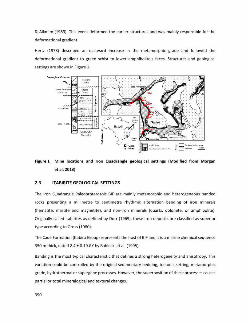
390
& Alkmim (1989). This event deformed the earlier structures and was mainly responsible for the
deformational gradient.
Hertz (1978) described an eastward increase in the metamorphic grade and followed the
deformational gradient to green schist to lower amphibolite’s faces. Structures and geological
settings are shown in Figure 1.
Figure 1 Mine locations and Iron Quadrangle geological settings (Modified from Morgan
et al. 2013)
2.3 ITABIRITE GEOLOGICAL SETTINGS
The Iron Quadrangle Paleoproterozoic BIF are mainly metamorphic and heterogeneous banded
rocks presenting a millimetre to centimetre rhythmic alternation banding of iron minerals
(hematite, martite and magnetite), and non-iron minerals (quartz, dolomite, or amphibolite).
Originally called itabirites as defined by Dorr (1969), these iron deposits are classified as superior
type according to Gross (1980).
The Cauê Formation (Itabira Group) represents the host of BIF and it is a marine chemical sequence
350 m thick, dated 2.4 ± 0.19 GY by Babinski et al. (1995).
Banding is the most typical characteristic that defines a strong heterogeneity and anisotropy. This
variation could be controlled by the original sedimentary bedding, tectonic setting, metamorphic
grade, hydrothermal or supergene processes. However, the superposition of these processes causes
partial or total mineralogical and textural changes.
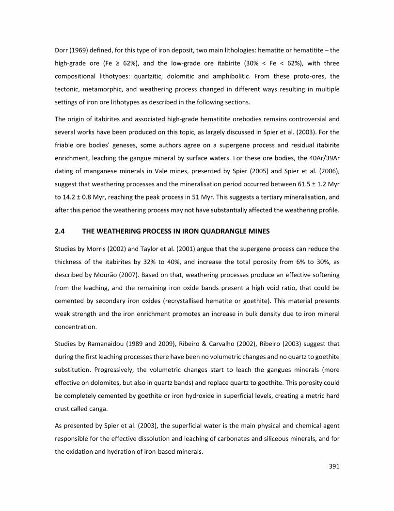
391
Dorr (1969) defined, for this type of iron deposit, two main lithologies: hematite or hematitite – the
high-grade ore (Fe ≥ 62%), and the low-grade ore itabirite (30% < Fe < 62%), with three
compositional lithotypes: quartzitic, dolomitic and amphibolitic. From these proto-ores, the
tectonic, metamorphic, and weathering process changed in different ways resulting in multiple
settings of iron ore lithotypes as described in the following sections.
The origin of itabirites and associated high-grade hematitite orebodies remains controversial and
several works have been produced on this topic, as largely discussed in Spier et al. (2003). For the
friable ore bodies’ geneses, some authors agree on a supergene process and residual itabirite
enrichment, leaching the gangue mineral by surface waters. For these ore bodies, the 40Ar/39Ar
dating of manganese minerals in Vale mines, presented by Spier (2005) and Spier et al. (2006),
suggest that weathering processes and the mineralisation period occurred between 61.5 ± 1.2 Myr
to 14.2 ± 0.8 Myr, reaching the peak process in 51 Myr. This suggests a tertiary mineralisation, and
after this period the weathering process may not have substantially affected the weathering profile.
2.4 THE WEATHERING PROCESS IN IRON QUADRANGLE MINES
Studies by Morris (2002) and Taylor et al. (2001) argue that the supergene process can reduce the
thickness of the itabirites by 32% to 40%, and increase the total porosity from 6% to 30%, as
described by Mourão (2007). Based on that, weathering processes produce an effective softening
from the leaching, and the remaining iron oxide bands present a high void ratio, that could be
cemented by secondary iron oxides (recrystallised hematite or goethite). This material presents
weak strength and the iron enrichment promotes an increase in bulk density due to iron mineral
concentration.
Studies by Ramanaidou (1989 and 2009), Ribeiro & Carvalho (2002), Ribeiro (2003) suggest that
during the first leaching processes there have been no volumetric changes and no quartz to goethite
substitution. Progressively, the volumetric changes start to leach the gangues minerals (more
effective on dolomites, but also in quartz bands) and replace quartz to goethite. This porosity could
be completely cemented by goethite or iron hydroxide in superficial levels, creating a metric hard
crust called canga.
As presented by Spier et al. (2003), the superficial water is the main physical and chemical agent
responsible for the effective dissolution and leaching of carbonates and siliceous minerals, and for
the oxidation and hydration of iron-based minerals.
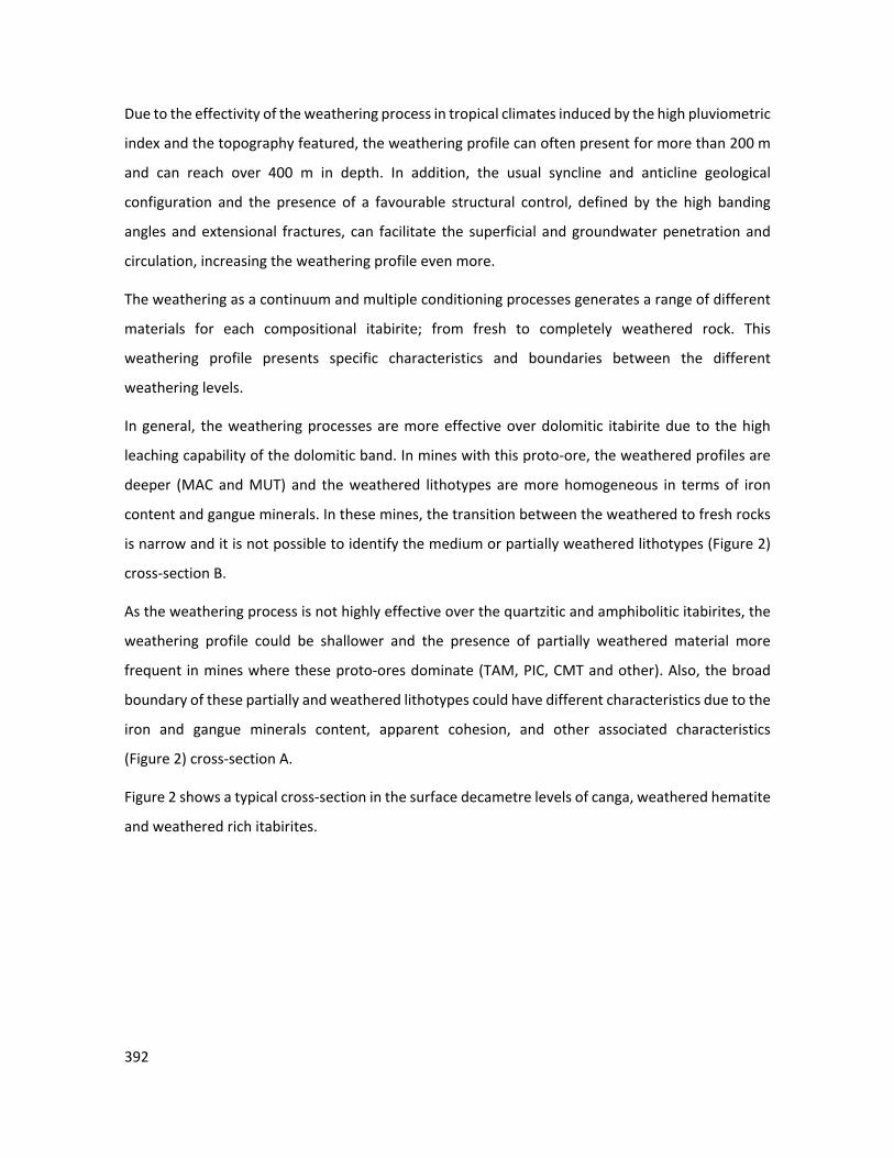
392
Due to the effectivity of the weathering process in tropical climates induced by the high pluviometric
index and the topography featured, the weathering profile can often present for more than 200 m
and can reach over 400 m in depth. In addition, the usual syncline and anticline geological
configuration and the presence of a favourable structural control, defined by the high banding
angles and extensional fractures, can facilitate the superficial and groundwater penetration and
circulation, increasing the weathering profile even more.
The weathering as a continuum and multiple conditioning processes generates a range of different
materials for each compositional itabirite; from fresh to completely weathered rock. This
weathering profile presents specific characteristics and boundaries between the different
weathering levels.
In general, the weathering processes are more effective over dolomitic itabirite due to the high
leaching capability of the dolomitic band. In mines with this proto-ore, the weathered profiles are
deeper (MAC and MUT) and the weathered lithotypes are more homogeneous in terms of iron
content and gangue minerals. In these mines, the transition between the weathered to fresh rocks
is narrow and it is not possible to identify the medium or partially weathered lithotypes (Figure 2)
cross-section B.
As the weathering process is not highly effective over the quartzitic and amphibolitic itabirites, the
weathering profile could be shallower and the presence of partially weathered material more
frequent in mines where these proto-ores dominate (TAM, PIC, CMT and other). Also, the broad
boundary of these partially and weathered lithotypes could have different characteristics due to the
iron and gangue minerals content, apparent cohesion, and other associated characteristics
(Figure 2) cross-section A.
Figure 2 shows a typical cross-section in the surface decametre levels of canga, weathered hematite
and weathered rich itabirites.
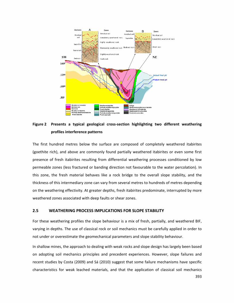
393
Figure 2 Presents a typical geological cross-section highlighting two different weathering
profiles interference patterns
The first hundred metres below the surface are composed of completely weathered itabirites
(goethite rich), and above are commonly found partially weathered itabirites or even some first
presence of fresh itabirites resulting from differential weathering processes conditioned by low
permeable zones (less fractured or banding direction not favourable to the water percolation). In
this zone, the fresh material behaves like a rock bridge to the overall slope stability, and the
thickness of this intermediary zone can vary from several metres to hundreds of metres depending
on the weathering effectivity. At greater depths, fresh itabirites predominate, interrupted by more
weathered zones associated with deep faults or shear zones.
2.5 WEATHERING PROCESS IMPLICATIONS FOR SLOPE STABILITY
For these weathering profiles the slope behaviour is a mix of fresh, partially, and weathered BIF,
varying in depths. The use of classical rock or soil mechanics must be carefully applied in order to
not under or overestimate the geomechanical parameters and slope stability behaviour.
In shallow mines, the approach to dealing with weak rocks and slope design has largely been based
on adopting soil mechanics principles and precedent experiences. However, slope failures and
recent studies by Costa (2009) and Sá (2010) suggest that some failure mechanisms have specific
characteristics for weak leached materials, and that the application of classical soil mechanics
394
principles does not enable the failure mechanisms to be fully understood, while rock mechanics
concepts are also not fully applicable.
The current approach used to develop slope stability analyses in these types of weak rocks is based
on limit equilibrium analyses and, in some special cases, these have been supported by numerical
models. The weak rock shear strength parameters for these designs are normally based on a limited
number of intact rock laboratory tests, such as triaxial and direct shear, and supported by adopted
rock mass classifications. While this approach has been mostly successful, it would appear that it
may be conservative. Despite that, there have been examples of large slope failures not captured
by these design approaches that have had significant negative impacts on mine production.
For future proposed open pit mines, there will be an increase in the percentage of hard/fresh rock
exposed in deeper Vale mines, which poses new challenges to the geotechnical team. They may
need to develop slope designs and evaluate possible failure mechanisms in hard rock by using
classical rock mechanics principles, breaking some paradigms established over past decades
operating mainly in weak rocks.
For these hard rocks, it is crucial to ensure a good evaluation of the intact rock strength, as well as
the geotechnical characteristics of the discontinuities in order to understand the slope deformation
behaviour for quite a complex arrangement of different rock strength materials.
It is also important to determine the geotechnical parameters for the partially weathered rocks
(a mixture of hard and weak rocks) and to develop a method to better define and map the
boundaries along the weathering continuum.
3 VALE ITABIRITES GEOLOGICAL AND GEOTECHNICAL CHARACTERISATION
In Vale mines, itabirites receive a local denomination defined by the iron ore, non-iron minerals
(gangue) contents and by the rock strength. Hematitite has the richest iron content (more than 62%
iron) and itabirite has the poorest iron content (less than 62%). Itabirites are reclassified by the main
gangue mineral found in three main lithotypes: quartz or quartzitic, dolomitic or carbonatic,
amphibolitic or goethitic. Others can be described as specularitic or martitic, but these are not so
prolific in Vale mines.
Hematitite and itabirites are also sub-divided using the rock hardness rated in Vale technological
crusher laboratory tests used to simulate the industrial process. This test consists of crushing a
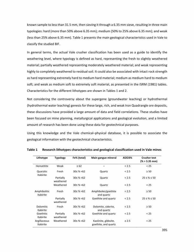
395
known sample to less than 31.5 mm, then sieving it through a 6.35 mm sieve, resulting in three main
typologies: hard (more than 50% above 6.35 mm); medium (50% to 25% above 6.35 mm); and weak
(less than 25% above 6.35 mm). Table 1 presents the main geological characteristics used in Vale to
classify the studied BIF.
In general terms, the actual Vale crusher classification has been used as a guide to identify the
weathering level, where typology is defined as hard, representing the fresh to slightly weathered
material; partially weathered representing moderately weathered material; and weak representing
highly to completely weathered to residual soil. It could also be associated with intact rock strength
as hard representing extremely hard to medium hard material; medium as medium hard to medium
soft; and weak as medium soft to extremely soft material, as presented in the ISRM (1981) tables.
Characteristics for the different lithotypes are shown in Tables 1 and 2.
Not considering the controversy about the supergene (groundwater leaching) or hydrothermal
(hydrothermal water leaching) genesis for these large, rich, and weak Iron Quadrangle ore deposits,
these discussions have provided a large amount of data and field correlations. These studies have
been focused on mine planning, metallurgical applications and geological evolution, and a limited
amount of research has been done using these data for geotechnical purposes.
Using this knowledge and the Vale chemical–physical database, it is possible to associate the
geological information with the geotechnical characteristics.
Table 1 Research lithotypes characteristics and geological classification used in Vale mines
Lithotype Typology Fe% (total) Main gangue mineral Al2O3% Crusher test (% > 3.35 mm)
Hematitite Weak ≥ 62 – < 2.5 < 25
Quarzitic Itabirite
Fresh 30≤ % <62 Quartz < 2.5 ≥ 50
Partially weathered
30≤ % <62 Quartz < 2.5 25 ≤ % ≤ 50
Weathered 30≤ % <62 Quartz < 2.5 < 25
Amphibolitic Itabirite
Fresh 30≤ % <62 Amphiboles/goethite and quartz
< 2.5 ≥ 50
Partially weathered
30≤ % <62 Goethite and quartz < 2.5 25 ≤ % ≤ 50
Dolomitic Itabirite
Fresh 30≤ % <62 Dolomite, siderite, and quartz
< 2.5 ≥ 50
Goethitic Itabirite
Partially weathered
30≤ % <62 Goethite and quartz < 2.5 < 25
Argillaceous Itabirite
Weathered 30≤ % <62 Kaolinite, gibbsite, goethite, and quartz
≥ 2.5 < 25
396
3.1 MAIN GEOLOGICAL CHARACTERISTICS
Typically, itabirites present a small mineralogical variety: hematite, martite, magnetite, specularite,
goethite and ochreous goethite are respectively the most important iron minerals; quartz, iron
dolomite, gibbsite and kaolinite are the main present gangue minerals; and talc, chlorite, pyrolusite
are the main accessory minerals. Several studies of Rosière et al. (1993, 1996 and 2001),
Lagoeiro (1998) and Pires (1995) describe the mineralogical and textural correlation with geological
association for several Iron Quadrangle mines.
For the researched lithotypes that represent approximately 75% of all typologies present in Vale’s
Iron Quadrangle mines, the main geological characteristics can be described as follows:
Weak hematitite (WHE) is the main supergene representative lithotype and the most extensive and
richest. It consists of thin (millimetre to centimetre) opaque/dark grey colour bands of hematite and
martite, with low resistance (friable) and high total porosity alternated by more consistent layers of
dark metallic bands of hematite and martite with higher relative resistance and lower total porosity.
The global porosity varies significantly from 25% to 30%, according to Costa et al. (2009), or even
higher, from 29% to 37% according to Ribeiro (2003). This lithotype represents a small
heterogeneity, but a sensitive anisotropy as defined by Costa (2009). In most cases, it represents
the tectonic foliation, but can also preserve the original banding.
Generally, these lithotypes are associated with synclines, and can be found in the lower surfaces
above the itabirites and can also occur in the shear zones and brittle failures presenting specularite
as presented in Costa (2009). Authigenic breccia is very common and can represent a load
deformation structure associated with the collapse. This collapse is imposed by the leaching process
and respective reduction in the itabirite volumes as exposed by Ribeiro (2003).
The grain size and shape of the minerals vary with the tectonical settings. The larger hematite
crystals are granuloblastic, the smaller are microplates, and the specularite presents lepidoblastic
texture.
In size, these iron minerals vary from 0.005 mm to 0.5 mm, with a maximum 0.1 mm as presented
in Rosière (2005).
The natural moisture content is closely linked to the rainy season, presenting an average of 15%.
The typical chemical composition is Fe (total) = 64%, SiO2+Al2O3<1%.
397
Fresh quartzitic itabirite (FQI) is the typical banded iron formation and more common itabirite as
originally described. The non-iron band was totally metamorphosed to quartz (originally chert
crystal), and the iron band is composed of hematite, martite and martitised magnetite. The typical
chemical composition presented in Vale mines is Fe (total) = 43%, SiO2 = 36% and Al2O3 = 0.3%.
The banding is generally folded and the microtexture of the quartz layers is granuloblastic to
lepidogranuloblastic. These crystals are euhedral due to the metamorphic level and their sizes range
from 10 µm to 120 µm, and the hematite layers present tabular and granular shapes and grain sizes
between 6 µm to 80 µm. They have a very low void ratio (e < 5%) and their moisture content is 10%
as presented by Santos (2007).
These rocks are commonly found in great depths but can also be observed in lowly deformed and
unfractured zones where it is possible to observe sedimentary structures and the primary bending.
Partially weathered quartzitic itabirite (PWQI) is the moderately weathered quartzitic itabirite,
presenting a mineralogical composition similar to the FQI, except by the extensive presence of
goethite. The quartz layers present a higher total porosity, and, in some instances, the quartz bands
can be disaggregated by differential leaching (some layers can reach e > 40%). Changes in mineral
texture or crystal size are not recognised in these materials. The leaching intensification determines
an increase in the total porosity, iron content and the percentage of goethite and ochreous goethite.
However, the intact rock strength and grain cohesion decreases, especially in the quartz bands.
Weathered quartzitic itabirite (WQI) describes the completely or totally weathered quartzitic
itabirite. With the increase in the weathering process, total porosity also increases, and bulk density
decreases due to the silica leaching.
For this weak rock, the original mineralogy remains with the addition of goethite and gibbsite
resulting from the weathering process. However, there is an important increase in the iron content
driven by the silica leaching. The typical chemical percentages are Fe (total) = 54%, SiO2 = 12% and
Al2O3 = 2%. Macroscopically, these rocks present a friable, dark metallic grey colour band of
hematite and martite, and white to yellow friable quartz bands with a minor amount of goethite.
The quartz bands present highly leaching layers (friable), where the total porosity easily reaches
40%.
398
Fresh amphibolitic itabirite (FAI) presents hematite, martite bands alternated with quartz, and
amphiboles (grunerite, tremolite, actonolithe and others) bands. The general band textures are
lepidogranuloblastic to granuloblastic and the crystal size is 30 µm on average.
The standard chemical composition is Fe (total) = 24%, SiO2 = 42% and Al2O3 = 0.4%. The original
mineralogy is preserved just in high depths where a typical brown-yellow colour is present. Usually,
the amphibole minerals change to fibrous goethite.
It is important to note that it is difficult to obtain fresh FAI which has not been influenced by some
mineral degradation specifically associated with the amphibole’s oxidation. The presence of
amphibole minerals is only observed in very high depth. In this paper, FAI is considered fresh if it fits
in the Vale crush test as a hard material and considered as slightly weathered material even if the
original amphiboles have changed to goethite.
Partially weathered goethitic itabirite (PWGI) represents the FAI partially weathered material and
the intact rock mass strength reduces significantly. The colour becomes yellow and it is noted that
there is an important increase in the total porosity and oxidation of iron ore minerals generating
goethite and ochreous goethite. These are shown in the several metres of the band between the
FAI and weathered goethite itabirite (WGI).
Weathered goethite itabirite (WGI) is characterised by the red and yellow colour caused by the high
goethite and ochreous goethite content presented mainly as cement. These also partially replace
the quartz crystal interlayer with friable quartz bands. They represent the totally weathered process
from the itabirites, quarzitic and amphibolitic, and are considered the more terrigenous lithotypes.
They are present in lower surface over WQI and MAI but can also be found in depth in open fractures
and shear zones.
Fresh dolomitic itabirite (FDI) is typically composed of millimetre to centimetre bands of euhedral
iron dolomite, responsible for the red colour and less percentage of iron carbonates and quartz.
These crystals vary from 2 µm to 15 µm. Non-iron bands are constituted of tabular hematite, martite
and martitised magnetite bands with crystal size varying from 5 µm to 20 µm. The most important
accessory minerals are sericite and chlorite. The total porosity is lower than 5% and the standard
chemical percentages are Fe (total) = 32%, CaO = 16% and MgO = 11%.
Weathered argillaceous itabirite (WAI) is characterised by the dark brown colour determined by
the high goethite and other clay mineral content, such as gibbsite and kaolinite. Spier (2005) argues
399
that they are formed by the effective leaching process over the dolomitic itabirites. The typical
banding is millimetre to centimetre composed of very fine crystals of martite hematite and goethite,
and bands of clay minerals. Some manganese minerals are common such as pyrolusite and
cryptomelanite. The total porosity is lower than 15% and the ρb = 2.64 t/m3. Chemical percentages
presented by WAI differ from the other weathered materials by the percentage of Al2O3 higher than
2.5%. However, the values of loss of ignition (LOI) (3.5 ≤ LOI < 5%) is the most important parameter
used to separate this typology from WGI (LOI ≥ 5%) and WQI (LOI < 3.5%).
The main visual characteristics of all evaluated lithotypes are presented in Figure 3, and Table 2
shows the main geotechnical characteristics.
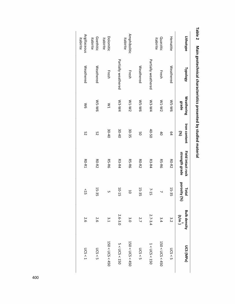
Ta ble 2 M
ain geotechnical characteristics presented by studied material
Lithotype Typology
Weathering grade
Iron content (%
) Field intact rock strength grade
Total porosity (%
) Bulk density
(t/m3)
UCS (M
Pa)
Hematite
Weathered
W5-W
6 64
R0-R2 15-35
3.2 U
CS < 5
Quarzitic
itabirite Fresh
W1-W
2 40
R5-R6 7
3.4 150 < U
CS < 450
Partially weathered
W3-W
4 40-50
R3-R4 7-15
2.7-3.4 1 < U
CS < 150
Weathered
W5-W
6 50
R0-R2 15-35
2.7 U
CS < 5
Amphibolitic
itabirite Fresh
W1-W
2 30-35
R5-R6 10
3.0 150 < U
CS < 450
Partially weathered
W3-W
4 30-40
R3-R4 10-15
2.6-3.0 5 < U
CS < 150
Dolomitic
itabirite Fresh
W1
30-40R5-R6
53.1
150 < UCS < 450
Goethitic itabirite
Weathered
W5-W
6 52
R0-R2 15-35
2.6 U
CS < 5
Argillaceous itabirite
Weathered
W6
52 R0-R1
<15 2.6
UCS < 1
400
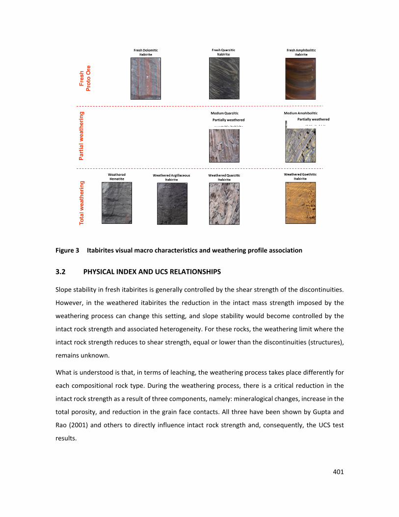
401
Figure 3 Itabirites visual macro characteristics and weathering profile association
3.2 PHYSICAL INDEX AND UCS RELATIONSHIPS
Slope stability in fresh itabirites is generally controlled by the shear strength of the discontinuities.
However, in the weathered itabirites the reduction in the intact mass strength imposed by the
weathering process can change this setting, and slope stability would become controlled by the
intact rock strength and associated heterogeneity. For these rocks, the weathering limit where the
intact rock strength reduces to shear strength, equal or lower than the discontinuities (structures),
remains unknown.
What is understood is that, in terms of leaching, the weathering process takes place differently for
each compositional rock type. During the weathering process, there is a critical reduction in the
intact rock strength as a result of three components, namely: mineralogical changes, increase in the
total porosity, and reduction in the grain face contacts. All three have been shown by Gupta and
Rao (2001) and others to directly influence intact rock strength and, consequently, the UCS test
results.
Partially weathered
quartzitic itabirite
Partially weathered
goethitic itabirite
402
UCS test results are largely used for fresh rock geotechnical evaluations. Several techniques have
been used to determine the intact rock strength. Some are based on laboratory (UCS), point load
test (PLT) or field tests (Schmidt hammer), and others are based on tactile visual or qualitative
estimation and its comparison with characteristic tables. Hack & Huisman (2002) and Vale’s
experiences suggest that, in many cases, the use of characteristic tables have proved to be more
than adequate and reliable to correlate with intact rock strength than the UCS values. However,
these simple estimation methods must be calibrated using laboratory testing in order to associate
the field strength estimation with the intact rock strength value.
The establishment of a standard characteristic table for Iron Quadrangle BIFs has been proposed by
several authors (Zenobio 2000; Zenobio & Zuquete 2004; Castro et al. 2013; and Araujo et al. 2014).
These authors generally adapt classical geomechanical classifications using, for example, specific
field procedures and tests, calibrated with laboratory tests.
For fresh rock in Vale mines, adapted strength field characterisation tables, crush tests and a limited
number of intact rock UCS tests have been used to determine the intact mass strength and guide
slope stability evaluation. Although this approach has been satisfactory, the increase of fresh rock
in deeper mines demands a higher level of information and more reliable data. Based on this
demand, several studies were initiated using the Vale geological/geotechnical database in order to
improve the data used for geotechnical purposes. The main approach has been to correlate the
available chemical and physical parameters from the different itabirites to the geotechnical index
proprieties. Proper correlations could be also used as a guide to predict BIF geotechnical
characteristics added to the existing techniques.
Index propriety interrelationships have been established worldwide for several rock types. Gupta
and Rao (1998 and 2001) and Irfan & Dearman (1978) mainly focused on granitic rocks and
established correlations between the physical proprieties of the rocks to the weathering process for
geotechnical evaluations. Even assuming geological differences between studied rocks and BIF,
these correlations are a useful guide for first consideration.
Specifically, for BIF, a similar access was established by Aylmer et al. (1978) evaluating the bulk
density, grade and porosity for Mount Tom Price iron ore and concluded that the iron grade and the
bulk density have a good correlation. However, the accuracy was largely affected by the high and
variable porosity.
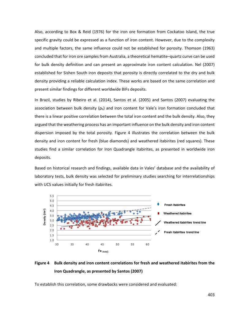
403
Also, according to Box & Reid (1976) for the iron ore formation from Cockatoo Island, the true
specific gravity could be expressed as a function of iron content. However, due to the complexity
and multiple factors, the same influence could not be established for porosity. Thomson (1963)
concluded that for iron ore samples from Australia, a theoretical hematite–quartz curve can be used
for bulk density definition and can present an approximate iron content calculation. Nel (2007)
established for Sishen South iron deposits that porosity is directly correlated to the dry and bulk
density providing a reliable calculation index. These works are based on the same correlation and
present similar findings for different worldwide BIFs deposits.
In Brazil, studies by Ribeiro et al. (2014), Santos et al. (2005) and Santos (2007) evaluating the
association between bulk density (ρb) and iron content for Vale’s iron formation concluded that
there is a linear positive correlation between the total iron content and the bulk density. Also, they
argued that the weathering process has an important influence on the bulk density and iron content
dispersion imposed by the total porosity. Figure 4 illustrates the correlation between the bulk
density and iron content for fresh (blue diamonds) and weathered itabirites (red squares). These
studies find a similar correlation for Iron Quadrangle itabirites, as presented in worldwide iron
deposits.
Based on historical research and findings, available data in Vales’ database and the availability of
laboratory tests, bulk density was selected for preliminary studies searching for interrelationships
with UCS values initially for fresh itabirites.
Figure 4 Bulk density and iron content correlations for fresh and weathered itabirites from the
Iron Quadrangle, as presented by Santos (2007)
To establish this correlation, some drawbacks were considered and evaluated:
404
• The ρb dispersion between the three main fresh itabirites presented a small range (2.7t/m3
to 4 t/m3).
• The ρb is highly influenced by porosity and this relationship is still not determined.
• The difficulty in obtaining fresh samples that do not present any type of weathering
change.
• The iron content variability due to the sample size.
In addition, as proposed by Hack & Huisman (2002), the use of UCS tests to determine the strength
of the material could present three main problems that could influence the results:
• The sample could include small discontinuities or flaws.
• The samples tend to have better mechanical characteristics associated with the sampling
technique (i.e. the best samples are selected).
• For anisotropic material, the results are sample orientation dependent.
To this list, one could add some geological features, such as intense folding, fill material, weathered
levels, veins, and other features that do not represent the typical rock mass material resulting to
invalid or biased results.
To avoid these drawbacks and in order to have more reliable results some assumptions were made
during the methodology development.
3.3 METHODOLOGY USED
In order to verify the correlation between the UCS values and the ρb of fresh itabirites, several
samples of FDIs, FQIs and FAIs were sent to Brazilian and Australian laboratories to undertake UCS
tests and ρb determinations. The laboratory UCS tests were undertaken in accordance with ASTM
D2938-95 (2002). Bulk density determination was based on the instantaneous water immersion
technique, while natural and dry mass per volume calculations were made using the samples’
dimensions.
For the test work undertaken in Australia, 15 samples were obtained from original 77.8 mm
diamond drill core subsampled for 20 mm diameter with lengths varying from 40 mm to 50 mm. For
the test work undertaken in Brazil, seven samples were used comprising the original 77.8 mm drill
cores with diameters varying from 50 mm to 76 mm and lengths from 110 mm to 205 mm.
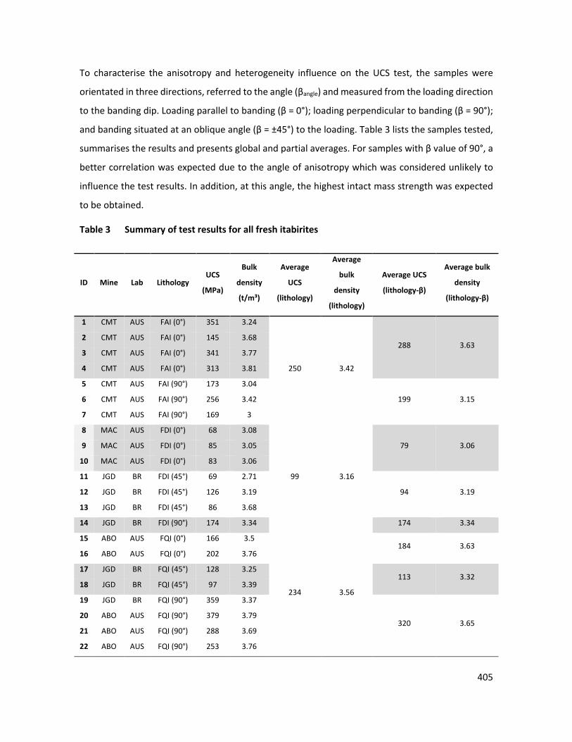
405
To characterise the anisotropy and heterogeneity influence on the UCS test, the samples were
orientated in three directions, referred to the angle (βangle) and measured from the loading direction
to the banding dip. Loading parallel to banding (β = 0°); loading perpendicular to banding (β = 90°);
and banding situated at an oblique angle (β = ±45°) to the loading. Table 3 lists the samples tested,
summarises the results and presents global and partial averages. For samples with β value of 90°, a
better correlation was expected due to the angle of anisotropy which was considered unlikely to
influence the test results. In addition, at this angle, the highest intact mass strength was expected
to be obtained.
Table 3 Summary of test results for all fresh itabirites
ID Mine Lab Lithology UCS
(MPa)
Bulk
density
(t/m³)
Average
UCS
(lithology)
Average
bulk
density
(lithology)
Average UCS
(lithology-β)
Average bulk
density
(lithology-β)
1 CMT AUS FAI (0°) 351 3.24
250 3.42
288 3.63 2 CMT AUS FAI (0°) 145 3.68
3 CMT AUS FAI (0°) 341 3.77
4 CMT AUS FAI (0°) 313 3.81
5 CMT AUS FAI (90°) 173 3.04
199 3.15 6 CMT AUS FAI (90°) 256 3.42
7 CMT AUS FAI (90°) 169 3
8 MAC AUS FDI (0°) 68 3.08
99 3.16
79 3.06 9 MAC AUS FDI (0°) 85 3.05
10 MAC AUS FDI (0°) 83 3.06
11 JGD BR FDI (45°) 69 2.71
94 3.19 12 JGD BR FDI (45°) 126 3.19
13 JGD BR FDI (45°) 86 3.68
14 JGD BR FDI (90°) 174 3.34 174 3.34
15 ABO AUS FQI (0°) 166 3.5
234 3.56
184 3.63 16 ABO AUS FQI (0°) 202 3.76
17 JGD BR FQI (45°) 128 3.25 113 3.32
18 JGD BR FQI (45°) 97 3.39
19 JGD BR FQI (90°) 359 3.37
320 3.65 20 ABO AUS FQI (90°) 379 3.79
21 ABO AUS FQI (90°) 288 3.69
22 ABO AUS FQI (90°) 253 3.76
406
The average values used in Vale for iron content, ρb, and total porosity (presented in Table 2) were
used as standard for these index propriety evaluations.
Considering the total porosity influence on bulk density results, studies of Box & Reid (1976), Aylmer
et al. (1978), Ribeiro (2003) and Santos et al. (2005), argued that the dispersion observed in the
results could be associated with this parameter variation. In this research stage, the influence of
total porosity was not evaluated.
However, for fresh itabirites, a minor total porosity variation is expected. This statement is
supported by Ribeiro et al. (2014) which argued that for FQI from the Conceição Mine, the total
porosity obtained by regression correlations presented values varying from 6.1% to 6.8%, and the
ρb varied from 3.3 t/ m3 to 3.9 t/ m3. These fit into the same range observed in the tested samples.
These values were confirmed by Moraes et al. (2014) who verified for the FQI from the Abóboras
Mine that the total porosity was 7.4% for a ρb = 3.07 t/ m3; for the Galinheiro and Sapecado Mines,
the total porosity was 9.2% for a ρb = 3.28 t/m3; and for FDI from the Gongo Soco Mine, the porosity
was 5.8% for a ρb = 3.11 t/m3. Based on these studies, for fresh itabirites, it is expected that there
will be a minor porosity influence on the results.
Considering the dispersion induced by the discontinuity presence and geological features, the
samples (pre-test) and the failure surface (post-test) were evaluated and photographed in order to
identify and characterise the main geological feature responsible for the failure, and that could have
affected ρb and/or UCS results.
This evaluation resulted in a sample divided into two groups:
• Typical, presenting proper lithotype characteristics such as,
FDI – typical red colour from dolomites bands and rhythmic millimetre to centimetre
banding.
FQI – typical white colour from quartz bands and rhythmic centimetre to millimetre
banding.
FAI – typical brown-yellow colour from goethite and quartz bands and rhythmic
centimetre banding.
• Not typical, and which do not fit into the required lithotype standards for intact mass strength
evaluation are geological features such as: intense folding, pre-existing close fracture,
brecciated, line of pores, veins (quartz or calcite), and specularite levels. It is important to note
407
that some of these geological features are commonly observed on these lithotypes and are
generally subordinate to the βangle. The tested samples, photographs and identification are
shown in Table 4.
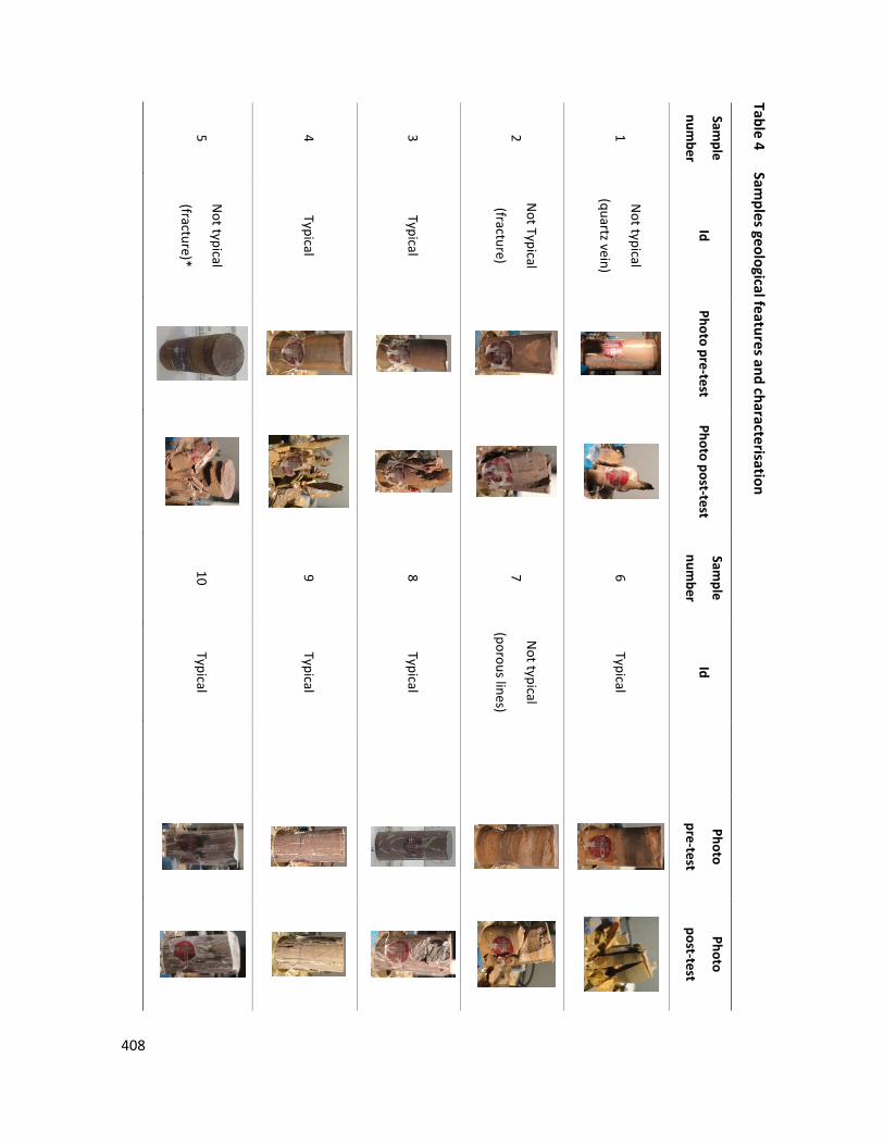
Table 4 Sam
ples geological features and characterisation
Sample
number
Id Photo pre-test
Photo post-test Sam
ple
number
Id Photo
pre-test
Photo
post-test
1 N
ot typical
(quartz vein) 6
Typical
2 N
ot Typical
(fracture) 7
Not typical
(porous lines)
3 Typical
8 Typical
4 Typical
9 Typical
5 N
ot typical
(fracture)* 10
Typical
408
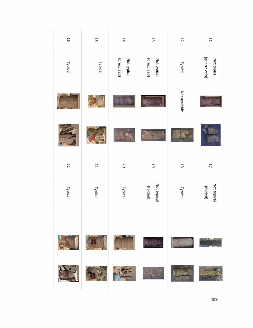
11 N
ot typical
(quartz vein) 17
Not typical
(folded)
12 Typical
Not avalable
18 Typical
13 N
ot typical
(brecciaed) 19
Not typical
(folded)
14 N
ot typical
(brecciaed) 20
Typical
15 Typical
21 Typical
16 Typical
22 Typical
409
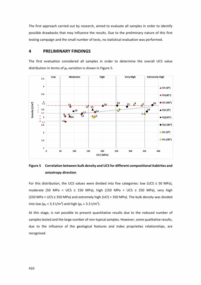
410
The first approach carried out by research, aimed to evaluate all samples in order to identify
possible drawbacks that may influence the results. Due to the preliminary nature of this first
testing campaign and the small number of tests, no statistical evaluation was performed.
4 PRELIMINARY FINDINGS
The first evaluation considered all samples in order to determine the overall UCS value
distribution in terms of ρb variation is shown in Figure 5.
Figure 5 Correlation between bulk density and UCS for different compositional itabirites and
anisotropy direction
For this distribution, the UCS values were divided into five categories: low (UCS ≤ 50 MPa),
moderate (50 MPa < UCS ≤ 150 MPa), high (150 MPa < UCS ≤ 250 MPa), very high
(250 MPa < UCS ≤ 350 MPa) and extremely high (UCS > 350 MPa). The bulk density was divided
into low (ρb < 3.3 t/m3) and high (ρb > 3.3 t/m3).
At this stage, is not possible to present quantitative results due to the reduced number of
samples tested and the large number of non-typical samples. However, some qualitative results,
due to the influence of the geological features and index proprieties relationships, are
recognised.
411
4.1 GEOLOGICAL FEATURES INFLUENCE
The presence of non-typical geological features presented in Table 4 showed some possible
drawbacks that may have interfered with the UCS and/or ρb results:
• Samples 2 and 5 present a previously closed fracture.
• Samples 13 and 14 present a brecciated material.
• Samples 17 and 19 presented folded banding.
• Samples 1 and 11 present quartz and calcite veins.
• Sample 7 presents large pore alignment.
By evaluating these sample results and correlating them with the observed geological features,
it is possible to identify some relationships:
• For samples 2, 7 and 5, due to the presence of fracture and alignment of large pores,
the UCS results were lower than expected, and for samples 7 and 5, a ρb reduction was
noted due to the presence of pores.
• For samples 1 and 11, due to the presence of quartz and calcite veins, a lower ρb was
evident. However, no considerable UCS reduction was observed.
• For samples 13 and 14, due to the presence of brecciated material, a higher ρb was
evident. However, it was not possible to discuss the UCS results.
• For samples 17 and 19, the presence of folded banding seems to not affect UCS or ρb
results.
Based on these evaluations, it was assumed that the presence of veins, closed fractures and
brecciaed material could produce biased data. For folding considerations, more evaluations are
necessary.
4.2 UCS AND BULK DENSITY FRESH ITABIRITE CORRELATION
Overall, the distribution of results presents a trend that is possible to see in Figure 5. However,
an important dispersion is noted and some considerations about this variation are:
• The FQI presented the higher range in UCS values, from extremely high to moderate.
However, the ρb was consistently high.
412
• The FAI ranged from very high to moderate UCS values with ρb varying from low to
high values. Excluding the non-typical samples 2, 5 and 7, the range reduced to very
high UCS and high- ρb values.
• The FAI and FQI average presented closer UCS and ρb values. However, considering the
anisotropy (β), FQI (90°) presented higher values.
• The low UCS results for FAI (90°) samples 7 and 5 could be partially associated with the
low ρb results.
• For the FDI, UCS values vary from high to moderate, presenting the lowest UCS average
compared to other lithotypes. However, ρb presents a high dispersion if the non-typical
samples 13 and 14 were included. Considering the anisotropy (β) influence in UCS and
ρb, the results for 90° samples presented higher values and were respectively lower for
45° and 0° for the two indices.
Evaluating the results per lithotype, it is possible to recognise some relationships about the index
parameters:
• For the FDI, the presence of brecciaed material increased the ρb and the UCS effects
were not well determined. However, these features must be considered separately
due to the directed result influence.
• For the FQI, the presence of folded banding tends to not influence the UCS values.
• For the FAI, the presence of large pores affects the UCS and ρb results.
• For all materials, closed fracture, and alignment of pores influence ρb and UCS results
especially when the β is different to 90°.
• For all materials, the presence of quartz and calcite veins directly influence the bulk
density values. However, the influence of these features for the UCS results is
associated with the anisotropy (β) direction.
5 CONCLUSION AND NEXT STEPS
Despite only 22 samples being tested from three lithotypes, the preliminary findings present the
same trend demonstrating similar results as obtained for other authors researching different
iron ore deposits. As Hack & Huisman (2002) previously proposed, this represents an important
interrelationship that could be used for the physical index characterisation of fresh itabirites.
413
These evaluations have emphasised the importance of identifying even the simplest geological
characteristics and/or structural features in order to have a proper correlation able to represent
the different types of fresh itabirites. Also, they suggest that the correlation between the UCS
and ρb could be an important pathway to infer the UCS values. The results outline the need for
more laboratory tests to support a statistically valid correlation from the Vale ρb database and
UCS test.
To achieve this primary aim, the number of UCS and ρb tests for fresh rock must be increased to
populate the graph and achieve the appropriate minimum sample size.
Further studies must be undertaken to determine the total porosity and iron content for the
fresh materials relationship and to investigate the influence of the heterogeneity associated
with the typical banding. After establishing these relationships for fresh materials, the study is
then likely to move forward to partially and completely weathered itabirites.
ACKNOWLEDGEMENTS
The authors thank Vale S.A. for permission to present this paper and their sponsorship of the
research undertaken by the Australian Centre for Geomechanics, The University of Western
Australia. The author’s appreciation extends to Vale colleagues Pedro Apolonio dos Santos, Diniz
Ribeiro, Fernando Machado, Eduardo Motta; and Ariel Hsieh and Eduardo Ansaloni for their
contributions.
REFERENCES
Aylmer, JA, Mathew, PJ & Wylie, AW 1978, ‘Bulk density of stratified iron ores and its
relationship to grade and porosity’, Proceedings of The Australasian Institute of Mining
and Metallurgy, The Australasian Institute of Mining and Metallurgy, Carlton, no. 265, pp.
9–17.
Araujo, TP, Amaral Jr, AF, Amaral, CG & Zenobio, AA 2014, ‘Weak rock mass strength in mining
slope, Minas Gerais state’, Proceedings of Rock Mechanics for Natural Resources and
Infrastructure, International Society for Rock Mechanics, Lisbon, pp. 125–130.
ASTM D2938-95 2002, Standard Test Method for Unconfined Compressive Strength of Intact
Rock Core Specimens, ASTM International, West Conshohocken.
Babinski, M, Chemale Jr, F & Van Schuss, WR 1995, ‘The Pb/Pb age of the Minas Supergroup
carbonate rocks, Quadrilátero Ferrífero, Brazil’, Precambrian Research, vol. 72, no. 3, pp.
235–245.
414
Box, GP & Reid, IW 1976, ‘Specific gravity and its relationship to chemical composition in iron
ore’, Proceedings of the Sampling Symposium, Australian Institute of Mining and
Metallurgy, Carlton, pp. 129–140.
Castro, LM, Carvalho, J & Sa, G 2013, ‘Discussion on how to classify and estimate strength of
weak rock masses’, Proceedings of the 2013 International Symposium on Slope Stability in
Open Pit Mining and Civil Engineering, Australian Centre for Geomechanics, Perth, pp.
205–217.
Chemale Jr, F, Rosière, CA & Endo, I 1994, ‘The tectonic evolution of the Quadrilátero Ferrífero,
Minas Gerais, Brazil’, Precambrian Research, vol. 65, no. 1, pp. 25–54.
Costa, TAV 2009, Geological and Geotechnical Characterization and Failure Mechanism of
Friable Hematite ore in Vale Iron Ore Mines. West of Iron Quadrangle – MG, Master’s
Thesis, Federal University of Ouro Preto, Ouro Preto.
Costa, TAV, Franca, PB & Figueiredo, RP 2009, ‘Geological and geotechnical characterization and
failure mechanism of friable hematite ore in Vale iron ore mines. West of Iron Quadrangle,
MG – Brazil, Proceedings of the 2009 International Symposium on Slope Stability,
University de los Andes, Santiago, pp. 120–128.
Dorr, JVN II 1969, Physiographic, Stratigraphic and Structural Development of the Quadrilátero
Ferrífero, Minas Gerais, Brazil, US Geological Survey Professional Paper, vol. 641-A, United
States Government Printing Office, Washington.
Gross, GA 1980, ‘A classification of iron formation based on depositional environments’, The
Canadian Mineralogist, vol. 18, pp. 215–222.
Gupta, AS & Rao, KS 1998, ‘Index properties of weathered rocks: inter-relationships and
applicability’, Bulletin of Engineering Geology and the Environment, vol. 57, no. 2, pp. 161–
172.
Gupta, AS & Rao, SK 2001, ‘Weathering indices and their applicability for crystalline rocks’,
Bulletin of Engineering Geology and the Environment, vol. 60, no. 3, pp. 201–221.
Hack, R & Huisman, M 2002, ‘Estimating the intact rock strength of a rock mass by simple means.
In engineering geology for developing countries’, Proceedings of 9th Congress of the
International Association for Engineering Geology and the Environment, International
Association for Engineering Geology and the Environment, pp. 16–20.
Hertz, N 1978, Metamorphic Rocks of the Iron Quadrangle, Minas Gerais, Brazil, US Geological
Survey Professional Paper, vol. 641-C, United States Government Printing Office,
Washington.
415
Irfan, TY & Dearman, WR 1978, ‘The engineering petrography of weathered granite in Cornwall,
England’, Quarterly Journal of Engineering Geology and Hydrogeology, vol. 11, no. 3,
pp. 233–244.
ISRM 1981a, Commission on Standardization of Laboratory and Field Test ‘Suggested Methods
for the Rock Characterization, Testing and Monitoring’, ET Brown (editor), Pergamon
Press, Oxford, UK, 211p.
Lagoeiro, LE 1998, ‘Magnetite and hematite transformation and the dissolution influence for
iron oxide’, Journal Metamorphic Geology, vol. 6, pp. 415–423.
Machado, N, Noce, CM, Oliveira, OD & Ladeira, EA 1989, ‘Archean and early Proterozoic iron
quadrangle geological evolution based on U-Pb geochronology’, Proceedings of the Minas
Gerais Geology Symposium, pp. 1–5.
Machado, N & Carneiro, MA 1992, ‘A major Archean tectonothermal event in the São Francisco
shield, Brazil: U-Pb evidence from the Quadrilátero Ferrífero, Minas Gerais’, Canadian
Journal of Earth Sciences, vol. 29, no. 11, pp. 2341–2346.
Marshak, S & Alkmim, FF 1989, ‘Proterozoic contraction/extension tectonics of the southern São
Francisco region, Minas Gerais, Brazil’, Tectonics, vol. 8, no. 3, pp. 555–571.
Moraes, IO, Ribeiro, DT, Santos, PA & Oliveira, FM 2014, Use of Normative Mineral Calculation
for Porosity and Density in Iron Quadrangle Compact Itabirites, Vale internal report.
Mourão, M 2007, Hydrogeological Characterization of Iron Quadrangle Cauê Aquifer, MG,
PhD Thesis, Federal University of Minas Gerais, Brazil.
Morris, RC 2002, ‘Iron genesis and post ore metasomatic at Mount Tom Price’, Proceedings Iron
Ore 2002, The Australasian Institute for Mining and Metallurgy, Carlton, pp. 3–12.
Morgan, R, Orberger, B, Rosière, CA, Wirth, R, Carvalho, CDM & Bellver-Baca, MT 2013, ‘The
origin of coexisting carbonates in banded iron formations: a micro-mineralogical study of
the 2.4 Ga Itabira Group, Brazil’, Precambrian Research, vol. 224, pp. 491–511.
Nel, D 2007, ‘A logical approach to determination of density and porosity values for iron ore
deposits’, Proceedings of Iron Ore 2007, The Australasian Institute of Mining and
Metallurgy, Carlton, pp. 141–146.
Noce, CM 1995, Iron Quadrangle Region Magmatic, Sedimentary and Metamorphic
Geochronological Events, Minas Gerais, PhD Thesis, University of São Paulo, São Paulo.
Pires, FRM 1995, ‘Textural and mineralogical variations during metamorphism of the Proterozoic
Itabira Iron Formation in the Quadrilátero Ferrífero, Minas Gerais, Brazil’, Annals of the
Brazilian Academy of Sciences, vol. 67, pp. 77–105.
Ramanaidou, E 1989, Geneses of Lateritic Deposit. Supergene Evolution of Proterozoic Iron Ore
from Capanema Mine, Minas Gerais, Brazil, PhD Thesis, University of Poitiers, Poitiers.
416
Ramanaidou, ER 2009, ‘Genesis of lateritic iron ore from banded iron-formation in the
Capanema mine (Minas Gerais, Brazil)’, Australian Journal of Earth Sciences, vol. 56,
no. 4. pp. 605–620.
Ribeiro, DT & Carvalho, RM 2002, ‘Simulation of weathered iron ore facies: integrating leaching
concepts and geostatistical models’, Proceedings of the Geostatistics Sessions of the 31st
International Geological Congress, Springer, Dordrecht, pp. 101–115.
Ribeiro, DT 2003, Banded Iron Formations: Supergene Enrichment: Disorder and Collapse
Structures, PhD Thesis, Federal University of Rio de Janeiro, Rio de Janeiro.
Ribeiro, DT, Santos, AP, Oliveira, MF & Moraes, OI 2014, Simulation and Estimative of Hard
Itabirites Density – Conceicao Mine - Final Report, Vale internal report.
Rosière, CA, Chemale, F, Jr & Quade, H 1993, ‘Iron Quadrangle iron ore microstructural analysis:
developed texture for an orgies model’, Proceedings of the Workshop on Geological Iron
Ore Structures, Geological Survey of Brazil, pp. 362–366
Rosière, CA, Quade, H, Siemes, H, Chemale, F, Jr & Resende de Souza, EM 1996,
‘A microstructural evolutional model for Iron Quadrangle iron ore. Part II – texture and
magnetic’, Geonomos, vol. 4, pp. 61–75.
Rosière, CA, Siemes, H, Quade, H, Brokmeier, HG and Jansen, EM 2001, ‘Microstructures,
textures and deformation mechanisms in hematite’, Journal of Structural Geology, vol. 23,
no. 9, pp. 1429–1440.
Rosière, CA 2005, MBR – Minerações Brasileiras Reunidas – The Geology of the MBR Iron Ore
Deposits, MBR internal report, Nova Lima.
Sá, G 2010, Lithostructural Characterization and Geomechanical Parametrization for N4E Slope
Failure Surfaces – Carajás; PA, PhD Thesis, Federal University of Ouro Preto, Ouro Preto.
Santos, PA, Kaneko, KM, Santos & GJL 2005, ‘Rock density test for CVRD – South Division’,
Proceedings of the VI Brazilian Iron Ore Symposium, Brazilian Mining, Materials and
Metallurgical Association, São Paulo, pp. 855–864.
Santos, PA 2007, ‘Variations rock density at Iron Quadrangle region’, Proceedings of the VIII
Brazilian Iron Ore Symposium, vol. 1, Brazilian Mining, Materials and Metallurgical
Association, São Paulo, pp. 200–211.
Spier, CA, de Oliveira, SMB & Rosière, CA 2003, ‘Geology and geochemistry of the Águas Claras
and Pico Iron Mines, Quadrilátero Ferrífero, Minas Gerais, Brazil’, Mineralium Deposita,
vol. 38, no. 6, pp. 751–774.
Spier, CA 2005, Geology and Geochemistry of the Águas Claras and Pico Iron Mines, Quadrilátero
Ferrífero, Minas Gerais, PhD Thesis, São Paulo University, São Paulo.
417
Spier, CA, Vasconcelos, PM & Oliveira, S 2006, ‘40Ar/39Ar geochronological constraints on the
evolution of lateritic iron deposits in the Quadrilátero Ferrífero, Minas Gerais, Brazil’,
Chemical Geology, vol. 234, no. 1, pp. 79–104.
Taylor, D, Dalstra, HJ, Harding, AE, Broadbent, GC & Barley, ME 2001, ‘Genesis of high-grade
hematite orebodies of Hamersley Province, Western Australia’, Economic Geology,
vol. 96, pp. 837–873.
Thomson, IA 1963, ‘The air comparison pycnometer for rapid iron determination’, Proceedings
of the Annual Conference, The Australasian Institute of Mining and Metallurgy, Carlton,
pp. 125–137.
Zenóbio, AA 2000, Geological – Geotechnical Natural Rock Slopes Evaluations using
Geomechanical Classifications: Ouro Preto CBD (MG) Scale 1:5.000, Master’s Thesis,
University of São Paulo, São Paulo.
Zenóbio, AA & Zuquete, LV 2004, ‘RQI (Rock Quality Index): proposal for the correction of RQD
parameter for natural rock slopes – Serra de Ouro Preto (Minas Gerais, Brazil)’,
Proceedings of the IX International Symposium on Landslide 2004, vol. 1, A.A. Balkema,
Rotterdam, pp. 101–106.

418
419
APPENDIX II
This paper was presented and published in 2015 at Slope Stability 2015 International Symposium
proceedings- SS03, Cape Town, South Africa.
WEATHERED BANDED IRON FORMATIONS IN VALE IRON ORE MINES ON
THE WESTERN SIDE OF THE IRON QUADRANGLE, BRAZIL: WEAK
HEMATITITE AND WEATHERED ARGILLACEOUS ITABIRITE GEOTECHNICAL
CHARACTERISTICS AND IMPLICATIONS OF MATRIC SUCTION EFFECTS ON
SLOPE STABILITY
COSTA, T.A.V.; DIGHT, P.M.; MERCER, K.; AND MARQUES, E.A.G.
ABSTRACT
Brazilian banded iron formations (BIF), locally known as itabirite, is the main host rock for iron
ore and hematitite is the high-grade ore in the Iron Quadrangle mines, Brazil. Their geneses are
controversial, but it is understood that weathering processes are principally responsible for
reducing the original high intact rock strength, and for generating deep weathered profiles with
low strength rocks commonly observed in Vale’s iron ore mines.
This paper presents a review of the geological and weathering characteristics and related
geomechanical and strength assessments of two important lithotypes commonly associated with
slope failure mechanisms in Vale mines: weathered argillaceous itabirite (WAI) and weak
hematitite (WHE). These studies are based on early research results from the PhD thesis being
undertaken by the lead author at the Australian Centre for Geomechanics, School of Civil,
Environmental and Mining Engineering, The University of Western Australia, sponsored by Vale
S.A.
The results show that minor changes in bulk density, texture, and the percentage of clay minerals
lead to distinct geomechanical characteristics in terms of plasticity, intact mass strength and
mainly matric suction effects. These changes influence both the shear strength and intact rock
behaviour and consequently the overall slope stability as shown in a preliminary insight into the
open pit slope design for short and long-term considerations.
420
1 INTRODUCTION
Vale S.A. Iron Quadrangle mines in Brazil generally exhibit weathering profiles that can reach
over 400 m in depth, and for these mines, the weathered rocks exhibit soil type behaviour. The
historical slope design approach and identification of possible failure mechanisms used by Vale
is largely based on applying classical soil mechanics principles as well as historical trial and error
experience. While this approach has been largely satisfactory, there are nevertheless several
key geotechnical issues that are still not well understood, and there have been continued
instances of large slope failures which have resulted in significant disruptions to the mines.
A PhD research project is currently being undertaken by the lead author of this paper at the
Australian Centre for Geomechanics, School of Civil, Environmental and Mining Engineering, The
University of Western Australia, sponsored by Vale S.A. The main objective of the thesis is to
investigate how the weathering process affects the geological and geotechnical characteristics
ranging from hard and fresh to weak and completely weathered rocks. This will ultimately
facilitate improved optimisation of final pit slope design and promote a better understanding of
potential failure mechanisms and, in turn, lead to a reduced risk of slope failure and hence, an
improvement of operational productivity and safety of Vale’s mines.
This paper shows the first results of this research and begins by presenting the geological setting
of the Iron Quadrangle mines in Brazil and goes on to summarise the key geological and
geotechnical characteristics of the weathered argillaceous itabirites and weak hematitites. The
general weathering process found at the mines is also described, followed by a review of the
implications of the weathering process on current slope stability. Material characterisation
studies which included laboratory tests for determination of bulk density, particle size
distributions (PSD), Atterberg limits, soil-water characteristic curves (SWCC) as well as saturated
and unsaturated direct shear tests are also presented. These test results are summarised and
evaluated to determine a correlation between key parameters and matric suction effects.
The results were applied in slope stability analysis using different pore pressure and matric
suction approaches. The paper ends with a discussion and conclusions on the possible
implications of these results on Vale’s mine slope stability.
421
2 GEOLOGICAL SETTING
2.1 LOCALISATION
The mines under study are part of Vale’s south ferrous division (DIFL) and comprise of fifteen
mines located in the centre of Minas Gerais, Brazil: Águas Claras (MAC), Mutuca (MUT), Mar
Azul (MAZ), Capão Xavier (CPX), Tamanduá (TAM), Capitão do Mato (CMT), Abóboras (ABO),
Galinheiro (GAL), Sapecado (SAP), Pico (PIC), Córrego do Feijão (CFJ), Jangada (JGD), João Pereira
(JPE), Alto Bandeira (BAN) and Fábrica (FAB). The location of these fifteen mines is shown in
Figure 1.
2.2 REGIONAL GEOLOGICAL SETTING
The focus area is in the western part of the Iron Quadrangle located in the southern border of
São Francisco Craton. The mines are sited along the Moeda and Don Bosco Synclines and Curral
Homocline ranges.
The Iron Quadrangle is delineated by a roughly quadrangular arrangement with
Paleoproterozoic banded iron formations (BIF) of the Minas Supergroup, as proposed by Dorr
(1969), composed of hundreds of metres of iron ore rich metamorphic rocks belonging to the
Itabira Group/Cauê Formation. The Minas Supergroup comprises, from bottom to top: the
Caraça, Itabira, Piracicaba and Sabará groups; superimposed by the Itacolomi Group.
Below that sequence are the Archean greenstone terrains of the Rio das Velhas Supergroup and
domes of Archean and Proterozoic crystalline rocks as studied by (Machado et al. 1989;
Machado & Carneiro 1992 and Noce 1995).
The regional structure is the result of two main deformational super-positional events as
described in Chemale Jr. et al. (1994). The first produced the nucleation of regional synclines in
the uplift of the gneissic domes during the Trans Amazonian Orogenesis (2.1–2 Gyr); and the
second is related to an east–west verging thrust fault belt of Pan African/Brazilian age (0.8–
0.6 Gyr) described by Marshak & Alkmim (1989). This event deformed the earlier structures and
was mainly responsible for the deformational gradient.
Locally the main iron ore deposits of DIFL/Vale are in the western low strain and green schist
metamorphic grade region as described by Hertz (1978). The geological settings are shown in
Figure 1.
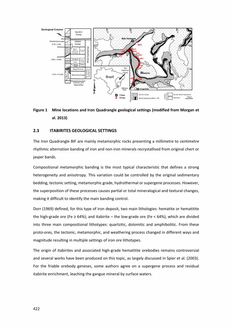
422
Figure 1 Mine locations and Iron Quadrangle geological settings (modified from Morgan et
al. 2013)
2.3 ITABIRITES GEOLOGICAL SETTINGS
The Iron Quadrangle BIF are mainly metamorphic rocks presenting a millimetre to centimetre
rhythmic alternation banding of iron and non-iron minerals recrystallised from original chert or
jasper bands.
Compositional metamorphic banding is the most typical characteristic that defines a strong
heterogeneity and anisotropy. This variation could be controlled by the original sedimentary
bedding, tectonic setting, metamorphic grade, hydrothermal or supergene processes. However,
the superposition of these processes causes partial or total mineralogical and textural changes,
making it difficult to identify the main banding control.
Dorr (1969) defined, for this type of iron deposit, two main lithologies: hematite or hematitite
the high-grade ore (Fe ≥ 64%); and itabirite – the low-grade ore (Fe < 64%), which are divided
into three main compositional lithotypes: quartzitic, dolomitic and amphibolitic. From these
proto-ores, the tectonic, metamorphic, and weathering process changed in different ways and
magnitude resulting in multiple settings of iron ore lithotypes.
The origin of itabirites and associated high-grade hematitite orebodies remains controversial
and several works have been produced on this topic, as largely discussed in Spier et al. (2003).
For the friable orebody geneses, some authors agree on a supergene process and residual
itabirite enrichment, leaching the gangue mineral by surface waters.
423
3 THE WEATHERING PROCESS IN IRON QUADRANGLE MINES
In this paper, the weathering process and supergene concentration sequence have been
considered as being the main phenomena responsible for the chemical and physical changes, as
described by Ribeiro (2003), Ribeiro & Carvalho (2002) and Spier (2005) and are directly
responsible for the reduction of the original itabirite strength. It should be noted that there are
other geological processes, such as tectonic events and metamorphism that could reduce the
original rock strength.
In terms of highly to completely weathered rocks, these low strength rocks could also be defined
as soft, friable or weak, and are invariably the result of alteration of the original fresh rock
imposed by weathering processes, particularly to completely leaching as proposed by Dorr
(1969, and 1973), Boulangé et al. (1997), Ribeiro & Carvalho (2002), Spier et al. (2006),
Ramanaidou (2009) and Ramanaidou and Morris (2010). However, metamorphic, and tectonic
events cannot be ignored as suggested by Pires (1979 and 1995).
Due to the effectivity of the weathering process in tropical climates induced by a high
temperature variation range and a high pluviometric index, in addition to the favourable
topography featured, the weathering profile can often present more than 200 m and reach over
400 m in depth. Also, the high permeability of BIF rocks, in association with structural feature
control such as syncline and anticline configurations and the presence of high banding angles
and extensional fractures, can facilitate the superficial and groundwater penetration and
circulation, increasing chemical and physical weathering and, thus, the weathering profile.
As presented by Ramanaidou & Morris (2010) the supergene iron enrichment and subsequent
strength reduction can be divided into two main processes. The supergene mimetic mechanism,
that occurs below the watertable as described by Morris et al. (1980) and Morris (2003) that is
associated with the structures, topography, and climate, and is responsible for producing deep
and large iron rich deposits. The second process was denominated as supergene lateritic
weathering and is a result of ganga minerals dissolution and iron reconcentration above the
watertable. This process produces several weathered profiles characterised by different relative
iron enrichment and ganga minerals composition.
Mineral changes are not the only effect of the weathering process. The total porosity increase
is also recognised as an important change observed in those rocks. Studies by Morris (2003) and
Taylor et al. (2001) argue that the supergene process can reduce the thickness of the BIF by 32 %
to 40%, and increase the total porosity from 6% to 30%, as described by Mourão (2007).
424
These studies suggest that the total porosity increase, and the mineral changes are the main
changes induced by the weathering processes that produce an effective softening in the original
fresh rocks. The leaching of the non-iron minerals provides the most important void increase on
non-iron bands while mineral changes are responsible for the total porosity increase on iron
bands. The remaining iron and non-iron bands present a high total porosity that could be
cemented by secondary iron oxides or hydroxides depending on various factors.
These materials present weak strength caused mainly by high total porosity; however, the
relative iron enrichment promotes an increase in bulk density due to iron minerals
concentration. As both parameters are important in determining the rock strength, it is crucial
to understand the balance between the iron ore concentration (which affects the original bulk
density) and the total porosity increase, in order to determine the most influential propriety
affecting rock strength.
As the weathering processes develop (close to the surface and in high water flow rate areas)
another important effect noted is the increase in percentage of hydroxides (ochreous goethite)
and clay minerals (kaolinite and gibbsite). The presence of these minerals in typical weathered
itabirites can change the geomechanical behaviour due to the increase in the rock plasticity or
filling the secondary porosity.
The weathering as a continuum and multiple conditioning processes generates a range of
different materials (lithotypes) for each compositional itabirites and the weathering profiles
present specific characteristics and boundaries between the different weathered levels. In
general, weathering processes are more effective over dolomitic itabirite due to the high
solubility of the iron dolomitic bands. In mines with this proto-ore (e.g. MAC, CPX and MUT), the
weathered profiles are generally deeper and the weathered lithotypes are more homogeneous
in terms of iron content and gangue minerals. In these mines, the transition between weathered
to fresh rocks is abrupt and it is difficult to identify the partially weathered material (Figure 2B).
As the weathering process is not highly effective over the quartzitic and amphibolitic itabirites
the presence of partially weathered material is more frequent and can reach tens of metres (e.g.
TAM, PIC and JPE). Also, the broad boundary of these partially weathered lithotypes could have
different characteristics for each type of compositional itabirite due to the gangue minerals
content, structures associated and topography (Figure 2, cross-section A).
Figure 2 shows a typical iron ore mine geological cross-section that presents on the surface
several metres of covering itabirites and hematitites. In mines where the geology and
topography are favourable to the supergene mimetic mechanism as proposed by Ramanaidou
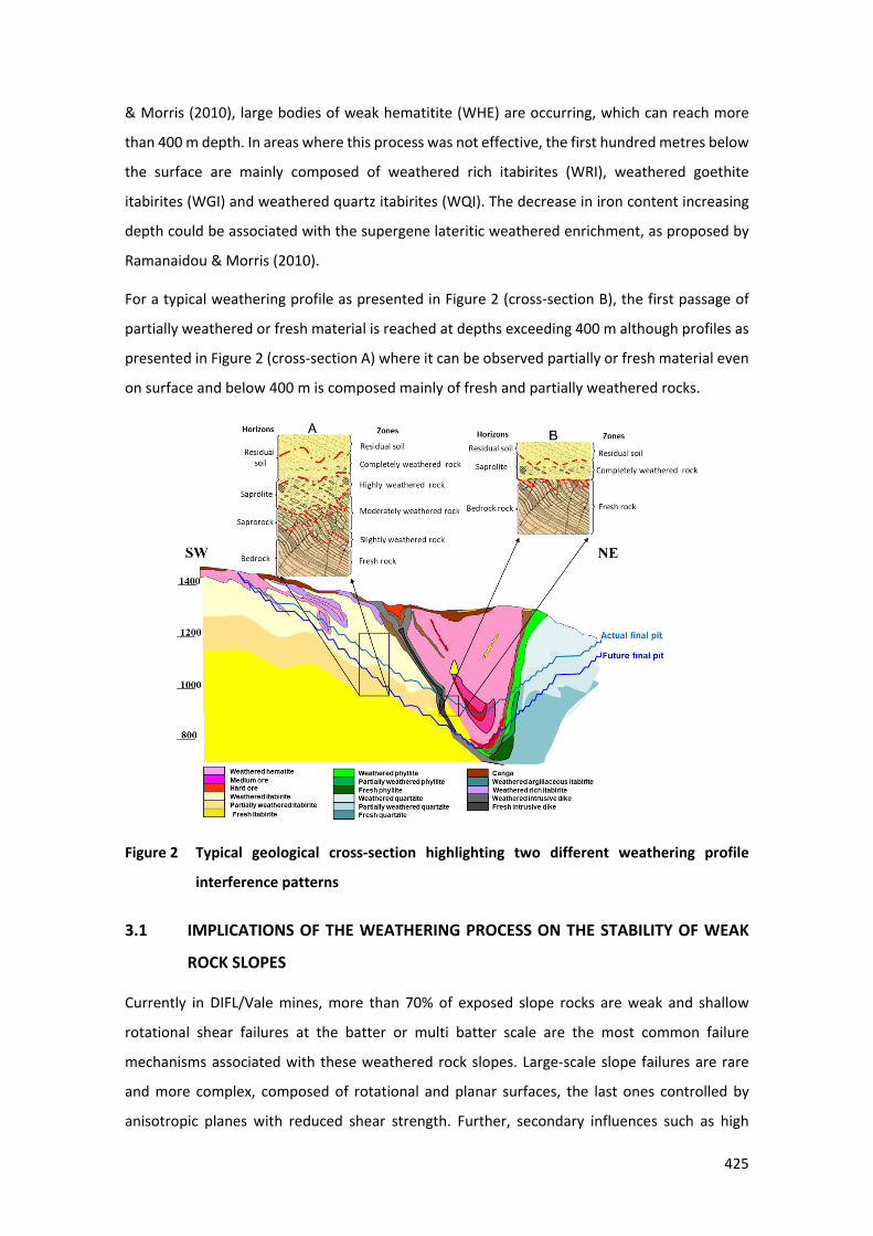
425
& Morris (2010), large bodies of weak hematitite (WHE) are occurring, which can reach more
than 400 m depth. In areas where this process was not effective, the first hundred metres below
the surface are mainly composed of weathered rich itabirites (WRI), weathered goethite
itabirites (WGI) and weathered quartz itabirites (WQI). The decrease in iron content increasing
depth could be associated with the supergene lateritic weathered enrichment, as proposed by
Ramanaidou & Morris (2010).
For a typical weathering profile as presented in Figure 2 (cross-section B), the first passage of
partially weathered or fresh material is reached at depths exceeding 400 m although profiles as
presented in Figure 2 (cross-section A) where it can be observed partially or fresh material even
on surface and below 400 m is composed mainly of fresh and partially weathered rocks.
Figure 2 Typical geological cross-section highlighting two different weathering profile
interference patterns
3.1 IMPLICATIONS OF THE WEATHERING PROCESS ON THE STABILITY OF WEAK
ROCK SLOPES
Currently in DIFL/Vale mines, more than 70% of exposed slope rocks are weak and shallow
rotational shear failures at the batter or multi batter scale are the most common failure
mechanisms associated with these weathered rock slopes. Large-scale slope failures are rare
and more complex, composed of rotational and planar surfaces, the last ones controlled by
anisotropic planes with reduced shear strength. Further, secondary influences such as high
426
stress concentrations at the toe of slopes and discontinuities may also act as contributing
factors.
The current approach used to undertake slope stability analyses in these types of weak rocks is
based on limit equilibrium analyses using the Mohr–Coulomb shear strength criterion and, in
some special cases, supported by numerical models. The shear strength parameters for these
designs are normally based on a limited number of intact rock laboratory tests which are mainly
saturated triaxial and direct shear and supported by adapted rock mass classifications. While
this approach has been mostly successful, it would appear from experience that they are
conservative. Despite that, there have been examples of large slope failures not captured by
these design approaches that have had significant negative impacts for mine production.
The situation is particularly challenging when considering the stratigraphic position and/or
tectonic settings of the weak rocks that are very often located at the toe of high slopes, where
the stress is concentrated. To address this issue, Vale geotechnical engineers have historically
designed a buttress of ore to be left at the toe of the wall, resulting in a loss of ore reserves, as
suggested in Costa et al. (2009).
In addition to the classical soil mechanics approaches, several weak material characteristics such
as total porosity, bulk density, grain size and shape, mineralogy, and anisotropy have been
evaluated and considered in relation to the observed slope stability behaviour. Describing and
correlating these parameters remains a key challenge to the author due to the difficulties
associated with sample acquisition, testing, scale effect and sample representativeness.
An important characteristic generally neglected for iron formations due to the high permeability
and low plasticity observed on those materials is the matric suction effect on slope stability.
However, a minor presence of clay minerals can influence the slope stability as presented by Lu
& Likos (2004) which argue that the matric suction contributes to the cohesion and increases
the shear strength of unsaturated soils. Studies by Grgic et al. (2005) on iron formations
suggested that an improvement on the strength and cohesion of partially saturated oolithic iron
ore can occur due to the negative pore water pressure effects.
It has been noted from work outside the mining industry that the shear strength of a soil with
negative porewater pressure can increase the stability of slopes, especially those having shallow
but steep surfaces as supported by Fredlund et al. (1978). So far, matric suction effects have not
been considered in Vale open pit slope stability evaluations where effective stress parameters
are obtained by conventional saturated laboratory testing. This approach seems to be adequate
for high pluviometric index areas where long-term slope stability is required. However, it tends
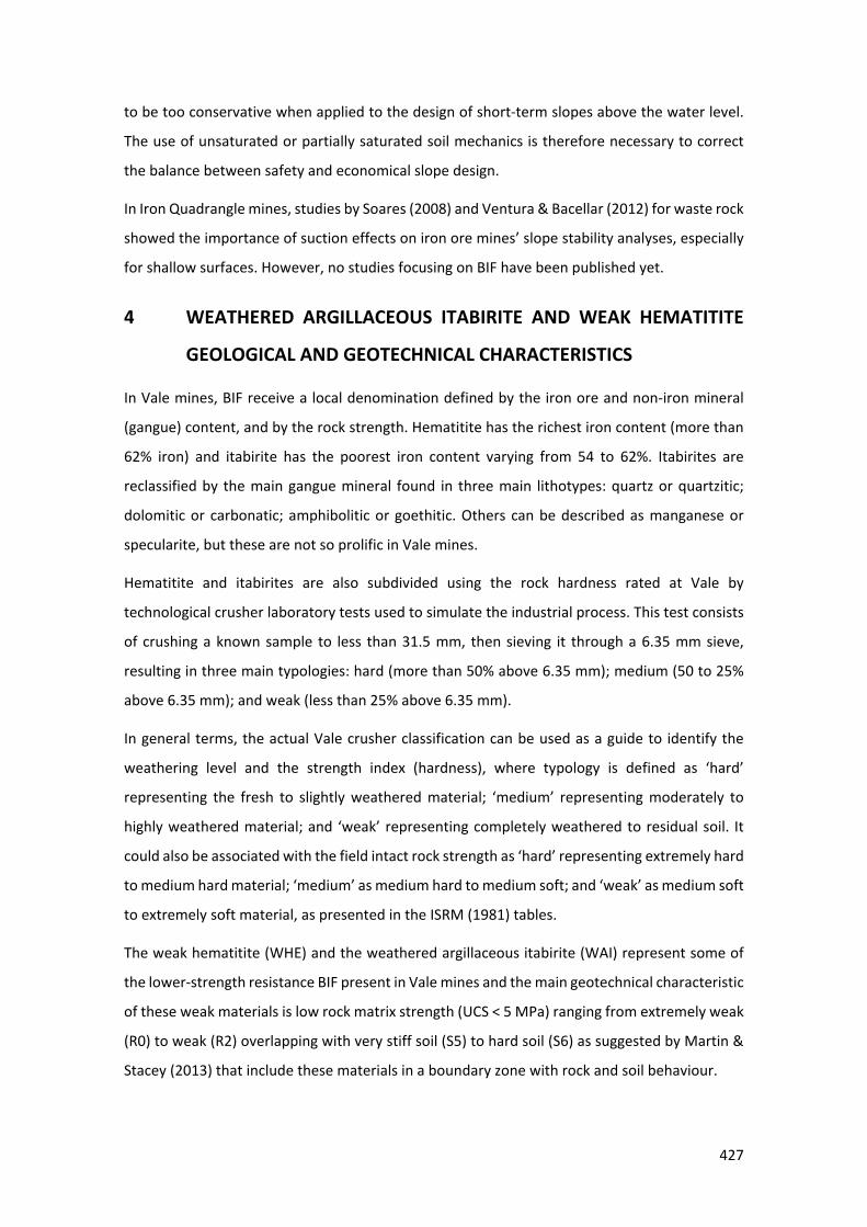
427
to be too conservative when applied to the design of short-term slopes above the water level.
The use of unsaturated or partially saturated soil mechanics is therefore necessary to correct
the balance between safety and economical slope design.
In Iron Quadrangle mines, studies by Soares (2008) and Ventura & Bacellar (2012) for waste rock
showed the importance of suction effects on iron ore mines’ slope stability analyses, especially
for shallow surfaces. However, no studies focusing on BIF have been published yet.
4 WEATHERED ARGILLACEOUS ITABIRITE AND WEAK HEMATITITE
GEOLOGICAL AND GEOTECHNICAL CHARACTERISTICS
In Vale mines, BIF receive a local denomination defined by the iron ore and non-iron mineral
(gangue) content, and by the rock strength. Hematitite has the richest iron content (more than
62% iron) and itabirite has the poorest iron content varying from 54 to 62%. Itabirites are
reclassified by the main gangue mineral found in three main lithotypes: quartz or quartzitic;
dolomitic or carbonatic; amphibolitic or goethitic. Others can be described as manganese or
specularite, but these are not so prolific in Vale mines.
Hematitite and itabirites are also subdivided using the rock hardness rated at Vale by
technological crusher laboratory tests used to simulate the industrial process. This test consists
of crushing a known sample to less than 31.5 mm, then sieving it through a 6.35 mm sieve,
resulting in three main typologies: hard (more than 50% above 6.35 mm); medium (50 to 25%
above 6.35 mm); and weak (less than 25% above 6.35 mm).
In general terms, the actual Vale crusher classification can be used as a guide to identify the
weathering level and the strength index (hardness), where typology is defined as ‘hard’
representing the fresh to slightly weathered material; ‘medium’ representing moderately to
highly weathered material; and ‘weak’ representing completely weathered to residual soil. It
could also be associated with the field intact rock strength as ‘hard’ representing extremely hard
to medium hard material; ‘medium’ as medium hard to medium soft; and ‘weak’ as medium soft
to extremely soft material, as presented in the ISRM (1981) tables.
The weak hematitite (WHE) and the weathered argillaceous itabirite (WAI) represent some of
the lower-strength resistance BIF present in Vale mines and the main geotechnical characteristic
of these weak materials is low rock matrix strength (UCS < 5 MPa) ranging from extremely weak
(R0) to weak (R2) overlapping with very stiff soil (S5) to hard soil (S6) as suggested by Martin &
Stacey (2013) that include these materials in a boundary zone with rock and soil behaviour.
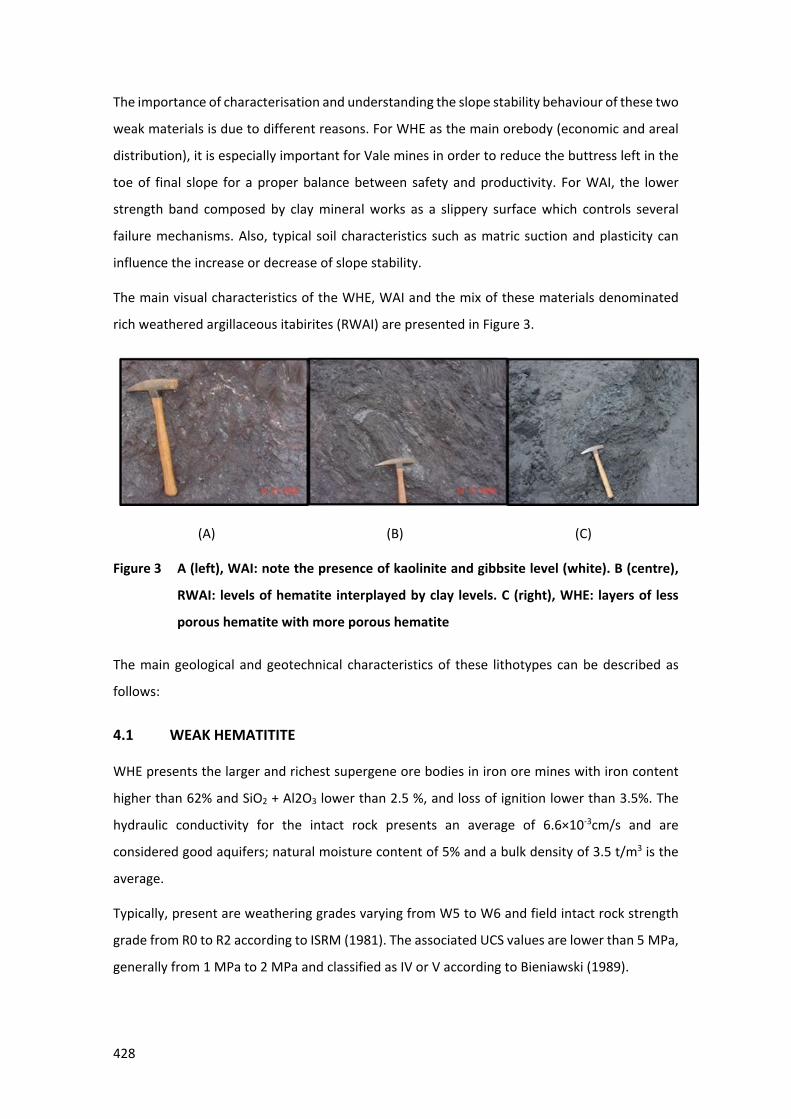
428
The importance of characterisation and understanding the slope stability behaviour of these two
weak materials is due to different reasons. For WHE as the main orebody (economic and areal
distribution), it is especially important for Vale mines in order to reduce the buttress left in the
toe of final slope for a proper balance between safety and productivity. For WAI, the lower
strength band composed by clay mineral works as a slippery surface which controls several
failure mechanisms. Also, typical soil characteristics such as matric suction and plasticity can
influence the increase or decrease of slope stability.
The main visual characteristics of the WHE, WAI and the mix of these materials denominated
rich weathered argillaceous itabirites (RWAI) are presented in Figure 3.
(A) (B) (C)
Figure 3 A (left), WAI: note the presence of kaolinite and gibbsite level (white). B (centre),
RWAI: levels of hematite interplayed by clay levels. C (right), WHE: layers of less
porous hematite with more porous hematite
The main geological and geotechnical characteristics of these lithotypes can be described as
follows:
4.1 WEAK HEMATITITE
WHE presents the larger and richest supergene ore bodies in iron ore mines with iron content
higher than 62% and SiO2 + Al2O3 lower than 2.5 %, and loss of ignition lower than 3.5%. The
hydraulic conductivity for the intact rock presents an average of 6.6×10⁻³cm/s and are
considered good aquifers; natural moisture content of 5% and a bulk density of 3.5 t/m3 is the
average.
Typically, present are weathering grades varying from W5 to W6 and field intact rock strength
grade from R0 to R2 according to ISRM (1981). The associated UCS values are lower than 5 MPa,
generally from 1 MPa to 2 MPa and classified as IV or V according to Bieniawski (1989).
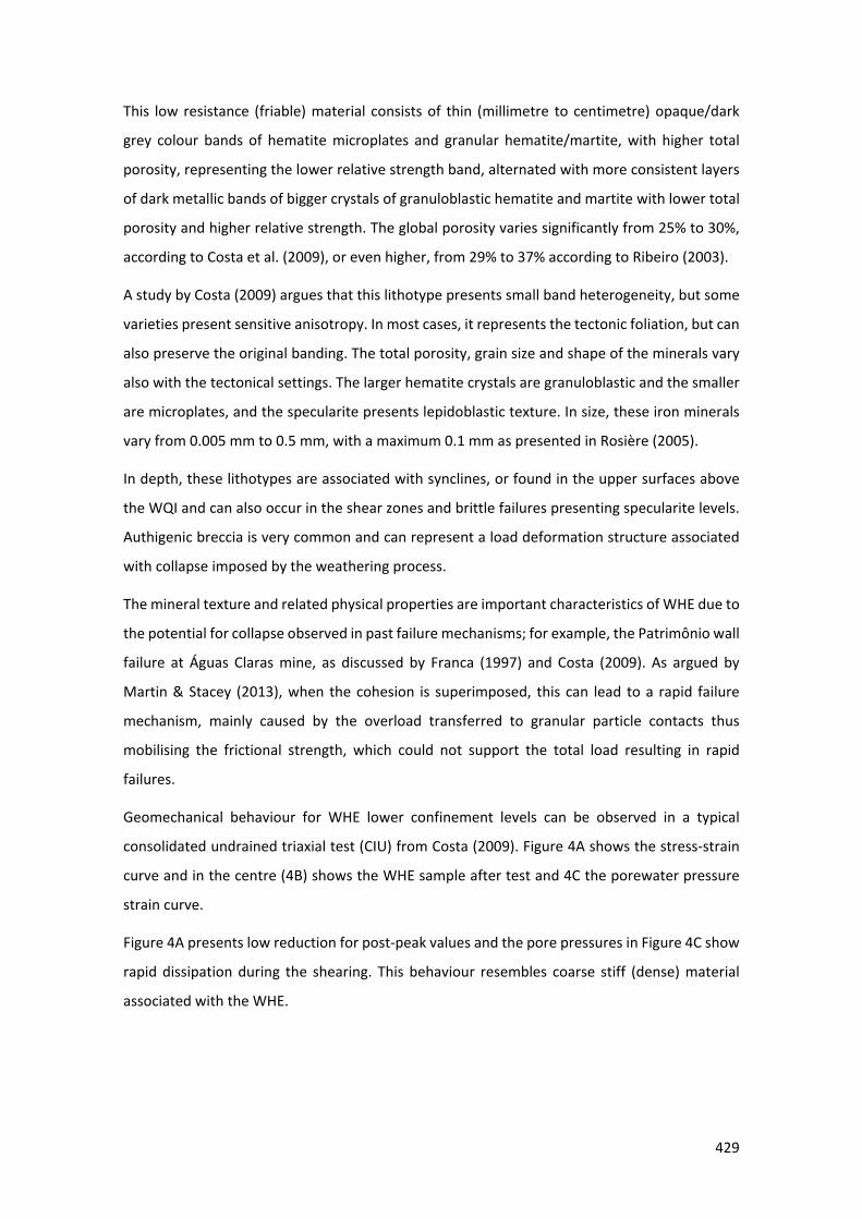
429
This low resistance (friable) material consists of thin (millimetre to centimetre) opaque/dark
grey colour bands of hematite microplates and granular hematite/martite, with higher total
porosity, representing the lower relative strength band, alternated with more consistent layers
of dark metallic bands of bigger crystals of granuloblastic hematite and martite with lower total
porosity and higher relative strength. The global porosity varies significantly from 25% to 30%,
according to Costa et al. (2009), or even higher, from 29% to 37% according to Ribeiro (2003).
A study by Costa (2009) argues that this lithotype presents small band heterogeneity, but some
varieties present sensitive anisotropy. In most cases, it represents the tectonic foliation, but can
also preserve the original banding. The total porosity, grain size and shape of the minerals vary
also with the tectonical settings. The larger hematite crystals are granuloblastic and the smaller
are microplates, and the specularite presents lepidoblastic texture. In size, these iron minerals
vary from 0.005 mm to 0.5 mm, with a maximum 0.1 mm as presented in Rosière (2005).
In depth, these lithotypes are associated with synclines, or found in the upper surfaces above
the WQI and can also occur in the shear zones and brittle failures presenting specularite levels.
Authigenic breccia is very common and can represent a load deformation structure associated
with collapse imposed by the weathering process.
The mineral texture and related physical properties are important characteristics of WHE due to
the potential for collapse observed in past failure mechanisms; for example, the Patrimônio wall
failure at Águas Claras mine, as discussed by Franca (1997) and Costa (2009). As argued by
Martin & Stacey (2013), when the cohesion is superimposed, this can lead to a rapid failure
mechanism, mainly caused by the overload transferred to granular particle contacts thus
mobilising the frictional strength, which could not support the total load resulting in rapid
failures.
Geomechanical behaviour for WHE lower confinement levels can be observed in a typical
consolidated undrained triaxial test (CIU) from Costa (2009). Figure 4A shows the stress-strain
curve and in the centre (4B) shows the WHE sample after test and 4C the porewater pressure
strain curve.
Figure 4A presents low reduction for post-peak values and the pore pressures in Figure 4C show
rapid dissipation during the shearing. This behaviour resembles coarse stiff (dense) material
associated with the WHE.
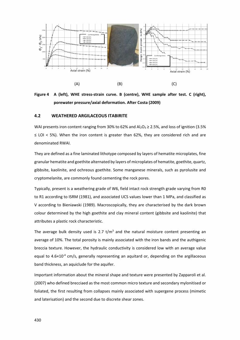
430
(A) (B) (C)
Figure 4 A (left), WHE stress-strain curve. B (centre), WHE sample after test. C (right),
porewater pressure/axial deformation. After Costa (2009)
4.2 WEATHERED ARGILACEOUS ITABIRITE
WAI presents iron content ranging from 30% to 62% and Al2O3 ≥ 2.5%, and loss of ignition (3.5%
≤ LOI < 5%). When the iron content is greater than 62%, they are considered rich and are
denominated RWAI.
They are defined as a fine laminated lithotype composed by layers of hematite microplates, fine
granular hematite and goethite alternated by layers of microplates of hematite, goethite, quartz,
gibbsite, kaolinite, and ochreous goethite. Some manganese minerals, such as pyrolusite and
cryptomelanite, are commonly found cementing the rock pores.
Typically, present is a weathering grade of W6, field intact rock strength grade varying from R0
to R1 according to ISRM (1981), and associated UCS values lower than 1 MPa, and classified as
V according to Bieniawski (1989). Macroscopically, they are characterised by the dark brown
colour determined by the high goethite and clay mineral content (gibbsite and kaolinite) that
attributes a plastic rock characteristic.
The average bulk density used is 2.7 t/m3 and the natural moisture content presenting an
average of 10%. The total porosity is mainly associated with the iron bands and the authigenic
breccia texture. However, the hydraulic conductivity is considered low with an average value
equal to 4.6×10⁻⁴ cm/s, generally representing an aquitard or, depending on the argillaceous
band thickness, an aquiclude for the aquifer.
Important information about the mineral shape and texture were presented by Zapparoli et al.
(2007) who defined brecciaed as the most common micro texture and secondary mylonitised or
foliated, the first resulting from collapses mainly associated with supergene process (mimetic
and laterisation) and the second due to discrete shear zones.
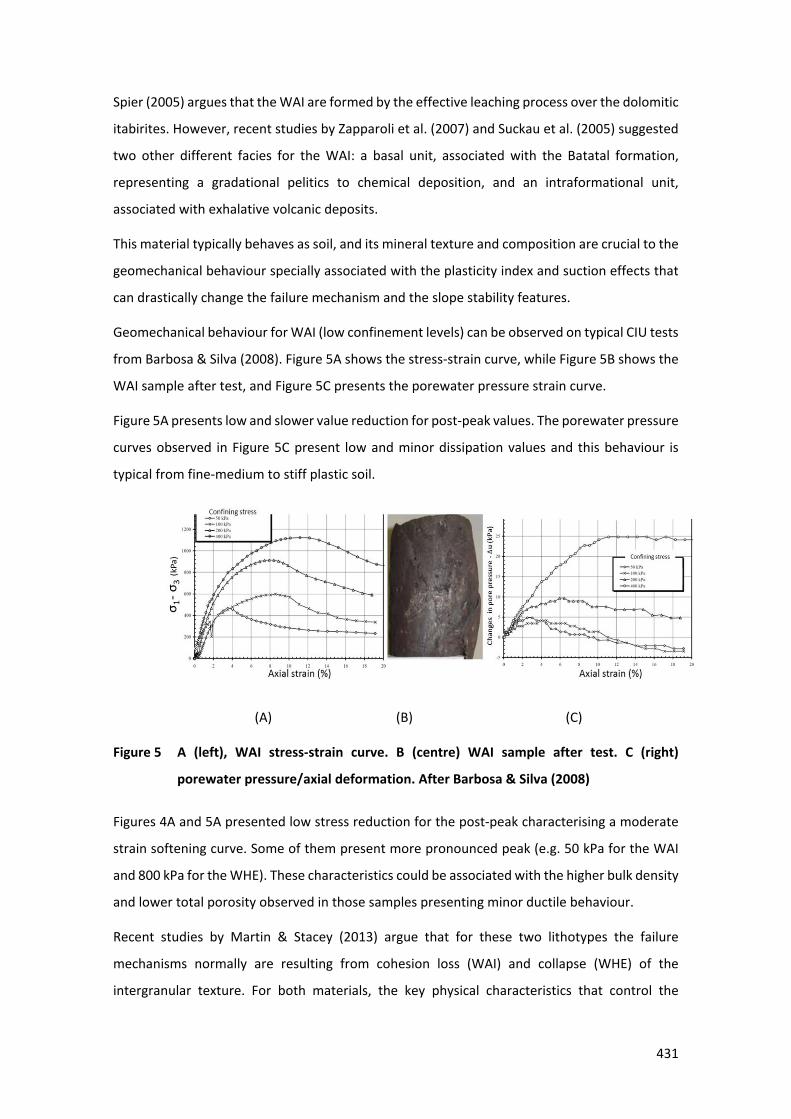
431
Spier (2005) argues that the WAI are formed by the effective leaching process over the dolomitic
itabirites. However, recent studies by Zapparoli et al. (2007) and Suckau et al. (2005) suggested
two other different facies for the WAI: a basal unit, associated with the Batatal formation,
representing a gradational pelitics to chemical deposition, and an intraformational unit,
associated with exhalative volcanic deposits.
This material typically behaves as soil, and its mineral texture and composition are crucial to the
geomechanical behaviour specially associated with the plasticity index and suction effects that
can drastically change the failure mechanism and the slope stability features.
Geomechanical behaviour for WAI (low confinement levels) can be observed on typical CIU tests
from Barbosa & Silva (2008). Figure 5A shows the stress-strain curve, while Figure 5B shows the
WAI sample after test, and Figure 5C presents the porewater pressure strain curve.
Figure 5A presents low and slower value reduction for post-peak values. The porewater pressure
curves observed in Figure 5C present low and minor dissipation values and this behaviour is
typical from fine-medium to stiff plastic soil.
(A) (B) (C)
Figure 5 A (left), WAI stress-strain curve. B (centre) WAI sample after test. C (right)
porewater pressure/axial deformation. After Barbosa & Silva (2008)
Figures 4A and 5A presented low stress reduction for the post-peak characterising a moderate
strain softening curve. Some of them present more pronounced peak (e.g. 50 kPa for the WAI
and 800 kPa for the WHE). These characteristics could be associated with the higher bulk density
and lower total porosity observed in those samples presenting minor ductile behaviour.
Recent studies by Martin & Stacey (2013) argue that for these two lithotypes the failure
mechanisms normally are resulting from cohesion loss (WAI) and collapse (WHE) of the
intergranular texture. For both materials, the key physical characteristics that control the
432
geomechanical behaviour were porosity and fabric (micro texture). These features are
intimately related to the mineral shape, PSD, void content, and density.
5 PRELIMINARY FINDINGS
5.1 LABORATORY TESTS
Laboratory tests were performed on eight samples and included bulk density, saturated and
unsaturated, single and multistage direct shear tests (DST); soil-water characteristic curve
(SWCC); particle size curve distribution (PSD) and Atterberg limits (ATT).These are performed on
original 77.8 mm cores casted with plaster diamond drill cores trimmed to 61.8 mm in order
obtain the necessary anisotropy angle (β) and ensure minimal sample disturbance.
The tests were undertaken in accordance with the following Australian standards: Direct Shear,
AS 1289.6.2.2 (AS 1998); PSD/Hydrometer, AS 1289.3. 6.3 (AS 2003) and AS 1289.3. 6.1 (AS
2009); Atterberg limits, AS 1289.0 (AS 2000); SPD/SG, AS 1289.3. 6.1 (AS 2009); Bulk Density,
AS 1289.3. 6.1 (AS 2009); Moisture Content, AS 1289.6.4.1 (AS 2016) and UCSCS, ASTM D2487-
00 (ASTM 2000).
The presence of anisotropy (βangle) due to banding was considered in all test work. These
materials were tested at β = 90° (perpendicular) and β = 0° (parallel) to the anisotropy plan. Also,
due to the heterogeneity promoted by the compositional metamorphic banding thickness and
related sample scale effects, represents a challenge to obtain samples with similar physical
characteristics (banding, total porosity, bulk density, etc). Therefore, some samples were
denominated as RWAI, defining a sample with ambiguous characteristics from WAI and WHE.
5.2 MATERIAL CHARACTERISATION
The section summarises the material characterisation from the test results. Table 1 lists the
Atterberg limits for the <425 μm fraction for each material and the associated USCS classification
of the samples according to ASTM D2487-00 (ASTM 2000). Natural moisture content is not
reported due to disturbance from long-term storage and transport. Table 1 also presents the
PSD and correlated parameters, and the dry density values.
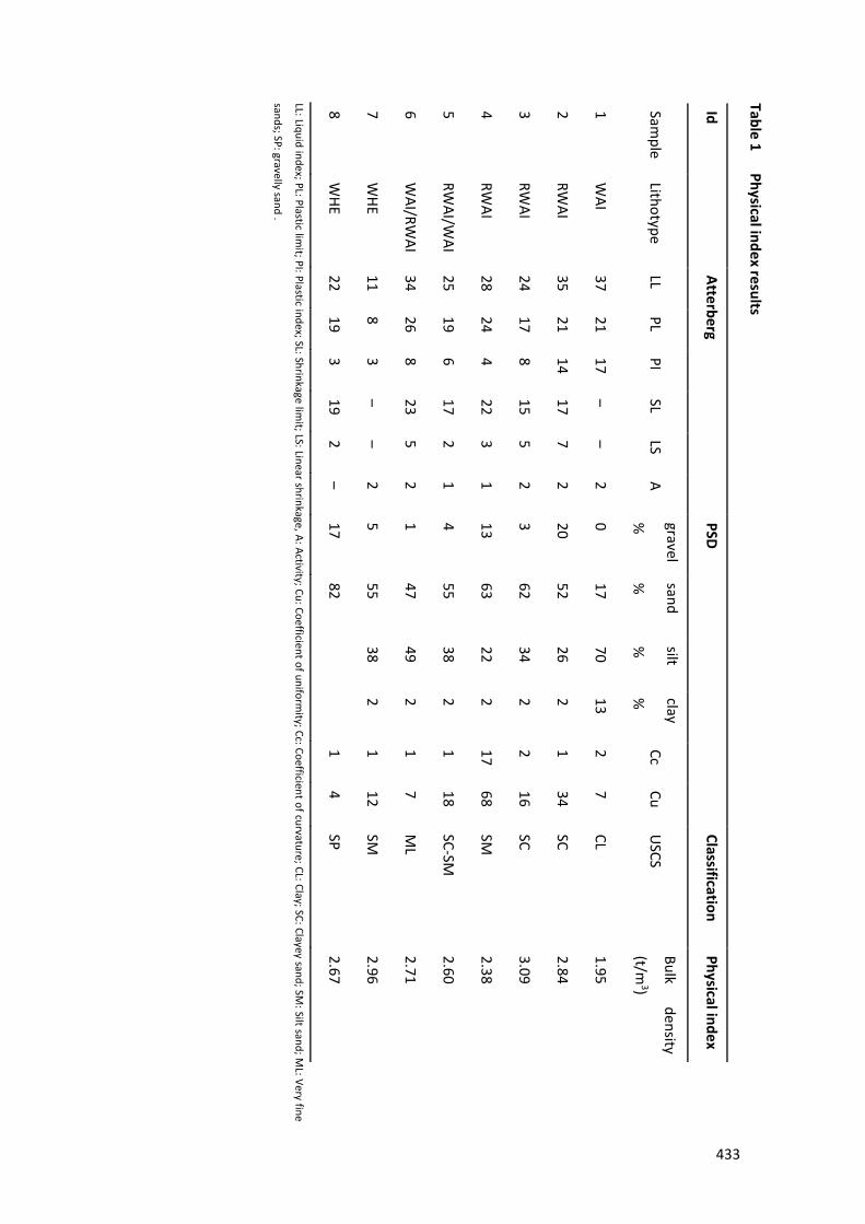
Ta ble 1 Physical index results
Id Atterberg
PSD
Classification Physical index
Sample
Lithotype LL
PL PI
SL LS
A gravel
%
sand
%
silt
%
clay
%
Cc Cu
USCS
Bulk density
(t/m3)
1 W
AI 37
21 17
––
2 0
17 70
13 2
7 CL
1.95
2 RW
AI 35
21 14
17 7
2 20
52 26
2 1
34 SC
2.84
3 RW
AI 24
17 8
15 5
2 3
62 34
2 2
16 SC
3.09
4 RW
AI 28
24 4
22 3
1 13
63 22
2 17
68 SM
2.38
5 RW
AI/WAI
25 19
6 17
2 1
4 55
38 2
1 18
SC-SM
2.60
6 W
AI/RWAI
34 26
8 23
5 2
1 47
49 2
1 7
ML
2.71
7 W
HE 11
8 3
––
25
55 38
2 1
12 SM
2.96
8 W
HE 22
19 3
19 2
–17
82 1
4 SP
2.67
LL: Liquid index; PL: Plastic limit; PI: Plastic index; SL: Shrinkage lim
it; LS: Linear shrinkage, A: Activity; Cu: Coefficient of uniformity; Cc: Coefficient of curvature; CL: Clay; SC: Clayey sand; SM
: Silt sand; ML: Very fine
sands; SP: gravelly sand .
433
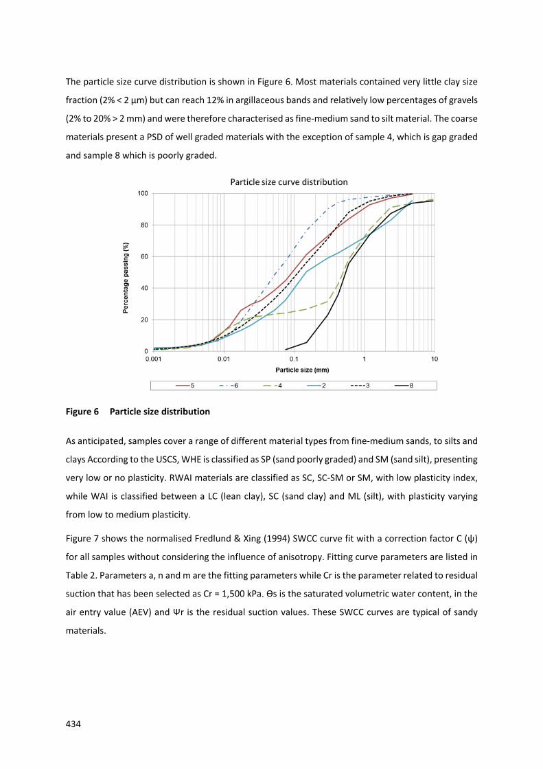
434
The particle size curve distribution is shown in Figure 6. Most materials contained very little clay size
fraction (2% < 2 μm) but can reach 12% in argillaceous bands and relatively low percentages of gravels
(2% to 20% > 2 mm) and were therefore characterised as fine-medium sand to silt material. The coarse
materials present a PSD of well graded materials with the exception of sample 4, which is gap graded
and sample 8 which is poorly graded.
Figure 6 Particle size distribution
As anticipated, samples cover a range of different material types from fine-medium sands, to silts and
clays According to the USCS, WHE is classified as SP (sand poorly graded) and SM (sand silt), presenting
very low or no plasticity. RWAI materials are classified as SC, SC-SM or SM, with low plasticity index,
while WAI is classified between a LC (lean clay), SC (sand clay) and ML (silt), with plasticity varying
from low to medium plasticity.
Figure 7 shows the normalised Fredlund & Xing (1994) SWCC curve fit with a correction factor C (ψ)
for all samples without considering the influence of anisotropy. Fitting curve parameters are listed in
Table 2. Parameters a, n and m are the fitting parameters while Cr is the parameter related to residual
suction that has been selected as Cr = 1,500 kPa. Өs is the saturated volumetric water content, in the
air entry value (AEV) and Ψr is the residual suction values. These SWCC curves are typical of sandy
materials.
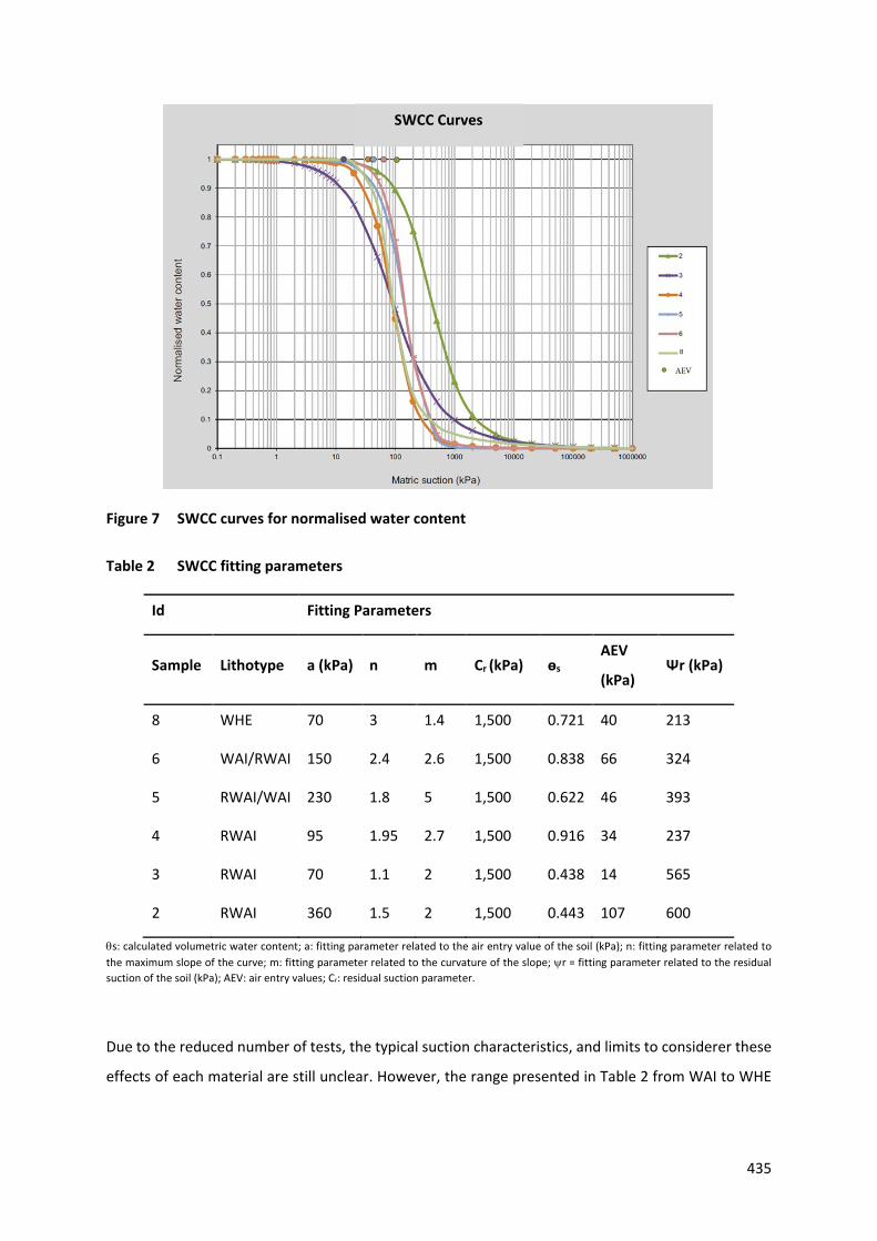
435
Figure 7 SWCC curves for normalised water content
Table 2 SWCC fitting parameters
Id Fitting Parameters
Sample Lithotype a (kPa) n m Cr (kPa) өs AEV
(kPa) Ψr (kPa)
8 WHE 70 3 1.4 1,500 0.721 40 213
6 WAI/RWAI 150 2.4 2.6 1,500 0.838 66 324
5 RWAI/WAI 230 1.8 5 1,500 0.622 46 393
4 RWAI 95 1.95 2.7 1,500 0.916 34 237
3 RWAI 70 1.1 2 1,500 0.438 14 565
2 RWAI 360 1.5 2 1,500 0.443 107 600
θs: calculated volumetric water content; a: fitting parameter related to the air entry value of the soil (kPa); n: fitting parameter related to the maximum slope of the curve; m: fitting parameter related to the curvature of the slope; ψr = fitting parameter related to the residual suction of the soil (kPa); AEV: air entry values; Cr: residual suction parameter.
Due to the reduced number of tests, the typical suction characteristics, and limits to considerer these
effects of each material are still unclear. However, the range presented in Table 2 from WAI to WHE
SWCC Curves
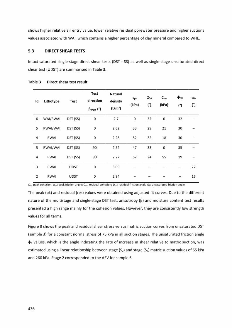
436
shows higher relative air entry value, lower relative residual porewater pressure and higher suctions
values associated with WAI, which contains a higher percentage of clay mineral compared to WHE.
5.3 DIRECT SHEAR TESTS
Intact saturated single-stage direct shear tests (DST - SS) as well as single-stage unsaturated direct
shear test (UDST) are summarised in Table 3.
Table 3 Direct shear test result
Id Lithotype Test
Test
direction
βangle (°)
Natural
density
(t/m3)
cpk
(kPa)
Φpk
(°)
Cres
(kPa)
φres
(°)
φb
(°)
6 WAI/RWAI DST (SS) 0 2.7 0 32 0 32 –
5 RWAI/WAI DST (SS) 0 2.62 33 29 21 30 –
4 RWAI DST (SS) 0 2.28 52 32 18 30 –
5 RWAI/WAI DST (SS) 90 2.52 47 33 0 35 –
4 RWAI DST (SS) 90 2.27 52 24 55 19 –
3 RWAI UDST 0 3.09 – – – – 22
2 RWAI UDST 0 2.84 – – – – 15
Cpk: peak cohesion; ɸpk: peak friction angle; Cres: residual cohesion; ɸres: residual friction angle ɸb: unsaturated friction angle.
The peak (pk) and residual (res) values were obtained using adjusted fit curves. Due to the different
nature of the multistage and single-stage DST test, anisotropy (β) and moisture content test results
presented a high range mainly for the cohesion values. However, they are consistently low strength
values for all terms.
Figure 8 shows the peak and residual shear stress versus matric suction curves from unsaturated DST
(sample 3) for a constant normal stress of 75 kPa in all suction stages. The unsaturated friction angle
φb values, which is the angle indicating the rate of increase in shear relative to matric suction, was
estimated using a linear relationship between stage (S2) and stage (S3) matric suction values of 65 kPa
and 260 kPa. Stage 2 corresponded to the AEV for sample 6.
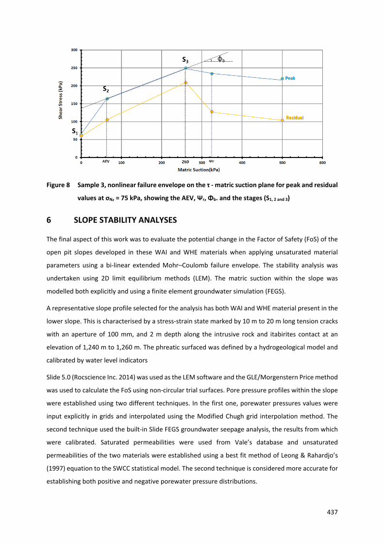
437
Figure 8 Sample 3, nonlinear failure envelope on the τ - matric suction plane for peak and residual
values at σN, = 75 kPa, showing the AEV, Ψr, Φb. and the stages (S1, 2 and 3)
6 SLOPE STABILITY ANALYSES
The final aspect of this work was to evaluate the potential change in the Factor of Safety (FoS) of the
open pit slopes developed in these WAI and WHE materials when applying unsaturated material
parameters using a bi-linear extended Mohr–Coulomb failure envelope. The stability analysis was
undertaken using 2D limit equilibrium methods (LEM). The matric suction within the slope was
modelled both explicitly and using a finite element groundwater simulation (FEGS).
A representative slope profile selected for the analysis has both WAI and WHE material present in the
lower slope. This is characterised by a stress-strain state marked by 10 m to 20 m long tension cracks
with an aperture of 100 mm, and 2 m depth along the intrusive rock and itabirites contact at an
elevation of 1,240 m to 1,260 m. The phreatic surfaced was defined by a hydrogeological model and
calibrated by water level indicators
Slide 5.0 (Rocscience Inc. 2014) was used as the LEM software and the GLE/Morgenstern Price method
was used to calculate the FoS using non-circular trial surfaces. Pore pressure profiles within the slope
were established using two different techniques. In the first one, porewater pressures values were
input explicitly in grids and interpolated using the Modified Chugh grid interpolation method. The
second technique used the built-in Slide FEGS groundwater seepage analysis, the results from which
were calibrated. Saturated permeabilities were used from Vale’s database and unsaturated
permeabilities of the two materials were established using a best fit method of Leong & Rahardjo’s
(1997) equation to the SWCC statistical model. The second technique is considered more accurate for
establishing both positive and negative porewater pressure distributions.
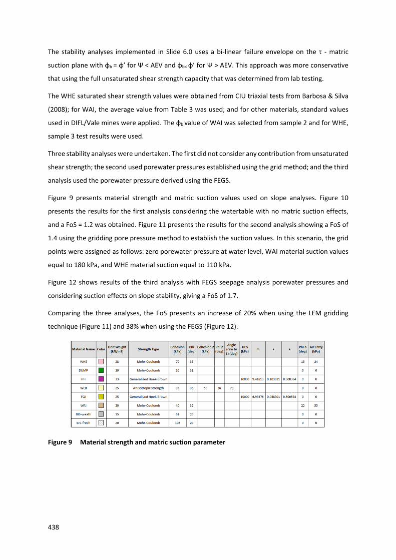
438
The stability analyses implemented in Slide 6.0 uses a bi-linear failure envelope on the τ - matric
suction plane with φb = φ’ for Ψ < AEV and φb< φ’ for Ψ > AEV. This approach was more conservative
that using the full unsaturated shear strength capacity that was determined from lab testing.
The WHE saturated shear strength values were obtained from CIU triaxial tests from Barbosa & Silva
(2008); for WAI, the average value from Table 3 was used; and for other materials, standard values
used in DIFL/Vale mines were applied. The φb value of WAI was selected from sample 2 and for WHE,
sample 3 test results were used.
Three stability analyses were undertaken. The first did not consider any contribution from unsaturated
shear strength; the second used porewater pressures established using the grid method; and the third
analysis used the porewater pressure derived using the FEGS.
Figure 9 presents material strength and matric suction values used on slope analyses. Figure 10
presents the results for the first analysis considering the watertable with no matric suction effects,
and a FoS = 1.2 was obtained. Figure 11 presents the results for the second analysis showing a FoS of
1.4 using the gridding pore pressure method to establish the suction values. In this scenario, the grid
points were assigned as follows: zero porewater pressure at water level, WAI material suction values
equal to 180 kPa, and WHE material suction equal to 110 kPa.
Figure 12 shows results of the third analysis with FEGS seepage analysis porewater pressures and
considering suction effects on slope stability, giving a FoS of 1.7.
Comparing the three analyses, the FoS presents an increase of 20% when using the LEM gridding
technique (Figure 11) and 38% when using the FEGS (Figure 12).
Figure 9 Material strength and matric suction parameter
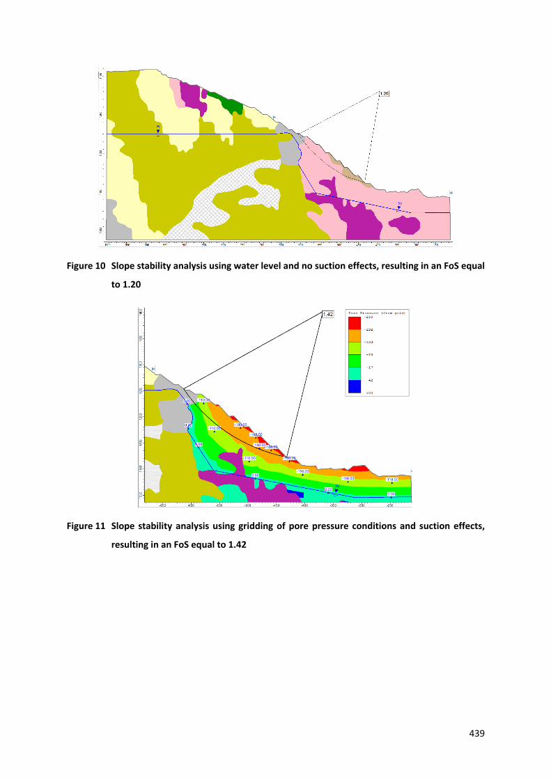
439
Figure 10 Slope stability analysis using water level and no suction effects, resulting in an FoS equal
to 1.20
Figure 11 Slope stability analysis using gridding of pore pressure conditions and suction effects,
resulting in an FoS equal to 1.42
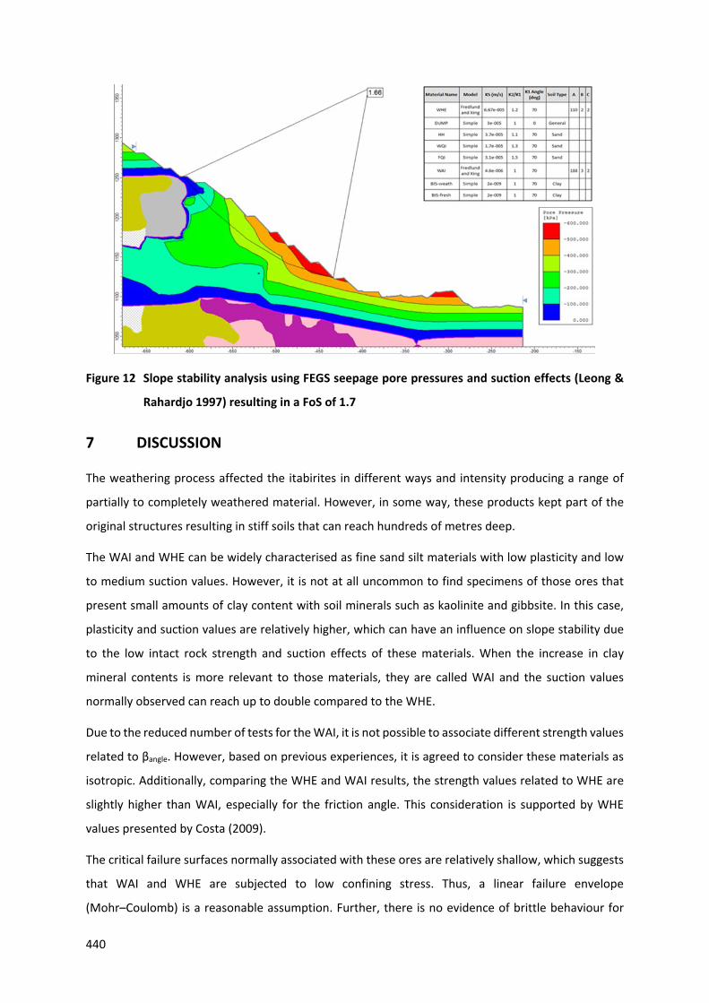
440
Figure 12 Slope stability analysis using FEGS seepage pore pressures and suction effects (Leong &
Rahardjo 1997) resulting in a FoS of 1.7
7 DISCUSSION
The weathering process affected the itabirites in different ways and intensity producing a range of
partially to completely weathered material. However, in some way, these products kept part of the
original structures resulting in stiff soils that can reach hundreds of metres deep.
The WAI and WHE can be widely characterised as fine sand silt materials with low plasticity and low
to medium suction values. However, it is not at all uncommon to find specimens of those ores that
present small amounts of clay content with soil minerals such as kaolinite and gibbsite. In this case,
plasticity and suction values are relatively higher, which can have an influence on slope stability due
to the low intact rock strength and suction effects of these materials. When the increase in clay
mineral contents is more relevant to those materials, they are called WAI and the suction values
normally observed can reach up to double compared to the WHE.
Due to the reduced number of tests for the WAI, it is not possible to associate different strength values
related to βangle. However, based on previous experiences, it is agreed to consider these materials as
isotropic. Additionally, comparing the WHE and WAI results, the strength values related to WHE are
slightly higher than WAI, especially for the friction angle. This consideration is supported by WHE
values presented by Costa (2009).
The critical failure surfaces normally associated with these ores are relatively shallow, which suggests
that WAI and WHE are subjected to low confining stress. Thus, a linear failure envelope
(Mohr–Coulomb) is a reasonable assumption. Further, there is no evidence of brittle behaviour for
441
WAI. These two aspects suggest that the friction angle must be the most important shear strength
parameter to be determined for these weak rock materials as also recognised by Martin & Stacey
(2013). However, for the WHE, due to the occurrence of some past events with deep failure surfaces,
more evaluations are necessary in order to understand the collapse potential of the mineral fabric.
This also contributes to the importance of determining the τ - matric suction plane of the extended
Mohr–Coulomb envelope for unsaturated conditions that can considerably increase the overall shear
strength resistance of weathered materials when evaluating the slope stability of these pit slopes.
When adopting the unsaturated shear strength, the variation of the unsaturated state of the materials
along critical surfaces from the wet to dry season needs to be carefully evaluated.
8 CONCLUSION AND NEXT STEPS
The preliminary results presented in this paper demonstrate a potential increase in the material shear
strength when considering the matric suction effects for WAI, which shows the potential benefit of
considering the negative porewater pressure distribution when evaluating slope stability.
The historical approach used in Vale mines which is based on saturated tests, effective strength
parameters and without considering matric suction effects, is suitable for long-term and post-closure
slope stability analyses. However, for short-term slope stability without water implications, this
approach is conservative.
To better evaluate the matric suction effects, more representative laboratory tests and more accurate
and calibrated groundwater simulations must be undertaken. The non-linearity of the failure envelope
on the τ - matric suction plane should be considered in the analysis. In addition, consideration of the
climate (seasonal) induced fluctuation of the near surface matric suction values (transient flow) as
well as the influence of the clay mineralogy must be evaluated to establish robust parameters for
undertaking sensitivity studies and achieving a high degree of reliability in the designs.
In terms of the next steps, further studies will be addressed to determine the porewater pressure
effects, physical parameters, and geomechanical relationship for a large number of WAI and WHE
samples. It will also be necessary to evaluate the matric suction effects for other weathered materials
(e.g. WQI and WGI) in order to establish a comprehensive understanding of the unsaturated shear
strength behaviour across the full range of the weak weathered iron formations in Vale S.A. iron
mines.
442
ACKNOWLEDGEMENTS
The author’s appreciation extends to Vale S.A. for supporting the research, the Australian Centre for
Geomechanics and Vale colleagues for their contribution, and special thanks to Victor Suckau and
Professor Waldyr Oliveira (EM/UFOP) for discussions about the nature of the WAI and suction effects.
REFERENCES
AS 1289.6.2.2 1998, Methods of Testing Soils for Engineering Purposes – Soil Strength and
Consolidation Tests – Determination of the Shear Strength of a Soil: Direct Shear Test Using a
Shear Box, Standards Australia, Sydney.
AS 1289.0 2000, Methods of Testing Soils for Engineering Purposes – General Requirements and List
Methods, Standards Australia, Sydney.
AS 1289.3. 6.3 2000, Methods of Testing Soils for Engineering Purposes – Soil Classification Tests –
Determination of the Particle Size Distribution of a Soil – Standard Method of Fine Analysis Using
a Hydrometer, Australia, Sydney.
AS 1289.3. 6.1 2009, Methods of Testing Soils for Engineering Purposes – Soil Classification Tests –
Determination of the Particle Size Distribution of a Soil – Standard Method of Analysis by Sieving,
Standards Australia, Sydney.
AS 1289.6.4.1 2016, Methods of Testing Soils of Engineering Purposes – Soil Strength and Consolidation
Tests – Determination of Compressive Strength of a Soil – Compressive Strength of a Specimen
Tested in Undrained Triaxial Compression Without Measurement of Pore Water Pressure,
Standards Australia, Sydney.
ASTM D2487-00 2000, Standard Classification of Soils for Engineering Purposes (Unified Soil
Classification System), American Society for Testing and Materials (ASTM), Philadelphia.
Barbosa, PSA & Silva, CHC 2008, Laboratory report 08-11 - Project: MBR (Capão Xavier mine), Federal
University of Viçosa, Viçosa, 286 pp.
Bieniawski, ZT 1989, Engineering Rock Mass Classifications, John Wiley & Sons, New York.
Boulangé, B, Carvalho, A, Varajão, CAC & Varajão, AF 1997, ‘The bauxite of the Quadrilátero Ferrífero’,
in A Carvalho, B Boulangé, AJ Melfi & Y Lucas (eds), Brazilian Bauxites, pp. 165–194.
Chemale Jr, F, Rosière, CA & Endo, I 1994, ’The tectonic evolution of the Quadrilátero Ferrífero, Minas
Gerais, Brazil’, Precambrian Research, vol. 65, no. 1, pp. 25–54.
Costa, TAV 2009, Geological and Geotechnical Characterization and Failure Mechanism of Friable
Hematite Ore in Vale Iron Ore Mines, West of Iron Quadrangle – MG, Master’s Thesis, Federal
University of Ouro Preto, Ouro Preto.
443
Costa, TAV, Franca, PB & Figueiredo, R, 2009, ‘Geological and geotechnical characterization and failure
mechanism of friable hematite Ore in Vale Iron Ore mines, West of Iron Quadrangle – MG,
Proceedings International Symposium on Slope Stability in Open Pit Mining and Civil
Engineering, Universidad de Los Andes, Santiago, pp. 120–128.
Dorr, JVN II 1969, Physiographic, Stratigraphic and Structural Development of the Quadrilátero
Ferrífero, Minas Gerais, Brazil, US Geological Survey Professional Paper, vol. 641-A, United
States Government Printing Office, Washington.
Dorr, JVN 1973, ‘Iron-formation in South America’, Economic Geology, vol. 68, no. 7, pp. 1005–1022.
Franca, PRB 1997, Analysis of Stability Using Limit Equilibrium and Numerical Methods with Case
Examples From the Águas Claras Mine, Brazil, Master’s Thesis, Queen´s University, Kingston.
Fredlund, DG, Morgenstern, NR & Widger, RA 1978, ‘The shear strength of unsaturated soils’,
Canadian Geotechnical Journal, vol. 5 no. 3. pp. 313–321.
Fredlund, DG & Xing, A 1994, ‘Equations for the soil-water characteristic curve’, Canadian
Geotechnical Journal, vol. 31, no. 4. pp. 521–532.
Grgic, D, Giot, R, Homand, F & Giraud, A 2005, ‘Effect of suction on the mechanical behaviour of iron
ore rock’, International Journal for Numerical and Analytical Methods in Geomechanics, vol. 29,
no. 8. pp. 789–827.
Hertz, N 1978, Metamorphic Rocks of the Iron Quadrangle, Minas Gerais, Brazil, US Geological Survey
Professional Paper, vol. 641-C, United States Government Printing Office, Washington.
ISRM 1981a, Commission on Standardization of Laboratory and Field Test ‘Suggested Methods for the
Rock Characterization, Testing and Monitoring’, E.T. Brown (editor), Pergamon Press, Oxford,
UK, 211p.
Leong, EC & Rahardjo, H 1997, ‘Permeability functions for unsaturated soils’, Journal of Geotechnical
and Geoenvironmental Engineering, vol. 123, no. 12. pp. 1118–1126.
Lu, N & Likos, WJ 2004, Unsaturated Soil Mechanics, John Wiley & Sons Inc, Hoboken.
Machado, N, Noce, CM, Oliveira, OAB de & Ladeira, EA 1989, ‘Archean and early Proterozoic iron
quadrangle geological evolution based on U-Pb geochronology’, Symposium on Geology from
Minas Gerais, Belo Horizonte, vol. 5. pp. 1–5.
Machado, N & Carneiro, MA 1992, ‘A major Archean tectonothermal event in the São Francisco shield,
Brazil: U-Pb evidence from the Quadrilátero Ferrífero, Minas Gerais’, Canadian Journal of Earth
Sciences, vol 29, no. 11. pp. 2341–2346.
Marshak, S & Alkmim, FF 1989, ‘Proterozoic contraction/extension tectonics of the southern São
Francisco region, Minas Gerais, Brazil’, Tectonics, vol. 8, no. 3. pp. 555–571.
444
Martin, CD & Stacey, PF 2013, 'Pit slopes in weathered and weak rocks', in PM Dight (ed.), Proceedings
of the 2013 International Symposium on Slope Stability in Open Pit Mining and Civil Engineering,
Australian Centre for Geomechanics, Perth, pp. 3-28,
https://doi.org/10.36487/ACG_rep/1308_0.1_Martin
Morgan, R, Orberger, B, Rosière, CA, Wirth, R, Carvalho, C da M & Bellver-Baca, MT 2013, ‘The origin
of coexisting carbonates in banded iron formations: A micro-mineralogical study of the 2.4Ga
Itabira Group, Brazil’, Precambrian Research, vol. 224, pp. 491–511,
https://doi.org/10.1016/j.precamres.2012.10.013
Morris, RC 1980, ‘A textural and mineralogical study of the relationship of iron ore to banded iron-
formation in the Hamersley Iron Province of Western Australia’, Economic Geology, vol. 75, no.
2. pp. 184–209.
Morris, RC 2003, ‘Iron ore genesis and post-ore metasomatism at Mount Tom Price’, Applied Earth
Science: Transactions of the Institutions of Mining and Metallurgy, Section B, vol. 112, no. 1, pp.
56–67.
Mourão, M 2007, Hydrogeological characterization of Iron Quadrangle Cauê aquifer, MG, PhD Thesis,
Federal University of Minas Gerais, Belo Horizonte.
Noce, CM 1995, Iron Quadrangle Region Magmatic, Sedimentary and Metamorphic Geochronological
Events, Minas Gerais, PhD Thesis, University of São Paulo, São Paulo.
Pires, FRM 1979, Structural Geology and Stratigraphy at the Junction of the Curral Anticline and the
Moeda Syncline, Quadrilátero Ferrífero, Minas Gerais, Brazil, PhD Thesis, Michigan
Technological University, Houghton.
Pires, FRM 1995, ‘Textural and mineralogical variations during metamorphism of the Proterozoic
Itabira Iron Formation in the Quadrilátero Ferrífero, Minas Gerais’, Brazil, Brazilian Academy of
Sciences Annual Report, vol. 67, pp. 77–105.
Ramanaidou, ER 2009, ‘Genesis of lateritic iron ore from banded iron-formation in the Capanema mine
(Minas Gerais, Brazil)’, Australian Journal of Earth Sciences, vol. 56, no. 4, pp. 605–620.
Ramanaidou, ER & Morris, RC 2010, ‘Comparison of supergene mimetic and supergene lateritic iron
ore deposits’, Applied Earth Science: Transactions of the Institutions of Mining and Metallurgy:
Section B, vol. 119, no. 1, pp. 35–39.
Ribeiro, DT & Carvalho, RM 2002, ‘Simulation of weathered iron ore facies: integrating leaching
concepts and geostatistical models’, in M Armstrong, C Bettini, N Champigny, A Galli & A
Remacre (eds), Proceedings of the Geostatistics Sessions of the 31st International Geological
Congress, Kluwer Academic Publishers, Dordrecht, pp. 101–115.
445
Ribeiro, DT 2003, Banded Iron Formations: Supergene Enrichment: Disorder and Collapse Structures,
PhD Thesis, Federal University of Rio de Janeiro, Rio de Janeiro.
Rocscience Inc. 2014, SLIDE 2D Limit Equilibrium Slope Stability Analysis, computer software,
Rocscience Inc., Toronto.
Rosière, CA 2005, MBR – Minerações Brasileiras Reunidas – The Geology of the MBR Iron Ore Deposits,
MBR internal report, Nova Lima.
Soares, EP 2008, Geotechnical and Mineralogical Characterisations of a Dolomitic Phyllite From the
Quadrilátero Ferrífero With a View to the Study of Slope Stability Incorporating Suction, Master’s
Thesis, Federal University of Ouro Preto, Ouro Preto.
Spier, CA, de Oliveira, SMB & Rosière, CA 2003, ‘Geology and geochemistry of the Águas Claras and
Pico Iron Mines, Quadrilátero Ferrífero, Minas Gerais, Brazil’, Mineralium Deposita, vol. 38,
no. 6, pp. 751–774.
Spier, CA 2005, Geology and Geochemistry of the Águas Claras and Pico Iron Mines, Quadrilátero
Ferrífero, Minas Gerais, PhD Thesis, São Paulo University, São Paulo.
Spier, CA, Vasconcelos, PM & Oliveira, S 2006, ‘40Ar/39Ar geochronological constraints on the
evolution of lateritic iron deposits in the Quadrilátero Ferrífero, Minas Gerais, Brazil’, Chemical
Geology, vol. 234, no. 1, pp. 79–104.
Suckau, VE, Suita, MTF, Zapparolli, AC, Spier, CA & Ribeiro, DT 2005, ‘Transitional pyroclastic, volcanic-
exhalative rocks to iron ores in Cauê formation, Tamanduá and Capitão do Mato mines: An
overview of metallogenic and tectonic aspects’, Proceedings of the III Sao Francisco Craton
Symposium, CBPM/UFBA/SBG, Salvador, pp. 343–346.
Taylor, D, Dalstra, HJ, Harding, AE, Broadbent, GC & Barley, ME 2001, ‘Genesis of high-grade hematite
orebodies of Hamersley Province, Western Australia’, Economic Geology, vol. 96. pp. 837–873.
Ventura, LC, Bacellar, LAP 2012, ‘Analysis of the influence of low conductivity formations on slope
stability of open-pit iron ore mines’, Proceedings of the 46th US Rock Mechanics/Geomechanics
Symposium, American Rock Mechanics Association, Alexandria.
Zapparoli, AC, Silva, RRR & Borges, AM 2007, Technological Project for Tamanduá Complex - PCTT-
Itabirites, MBR internal report, pp.1–8.

446
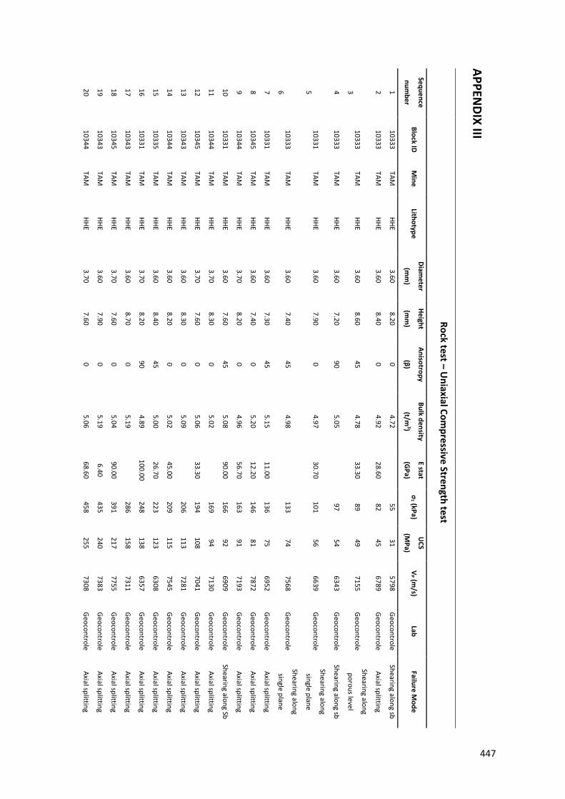
APPENDIX III
Rock test – Uniaxial Com
pressive Strength test
Sequence
number
Block ID M
ine Lithotype
Diameter
(mm
)
Height
(mm
)
Anisotropy
(β)
Bulk density
(t/m3)
E stat
(GPa)
σ1 (kPa)
UCS
(MPa)
VP (m
/s) Lab
Failure Mode
1 10333
TAM
HHE 3.60
8.20 0
4.72 55
31 5798
Geocontrole Shearing along sb
2 10333
TAM
HHE 3.60
8.40 0
4.92 28.60
82 45
6789 Geocontrole
Axial splitting
3 10333
TAM
HHE 3.60
8.60 45
4.78 33.30
89 49
7155 Geocontrole
Shearing along
porous level
4 10333
TAM
HHE 3.60
7.20 90
5.05 97
54 6343
Geocontrole Shearing along sb
5 10331
TAM
HHE 3.60
7.90 0
4.97 30.70
101 56
6639 Geocontrole
Shearing along
single plane
6 10333
TAM
HHE 3.60
7.40 45
4.98 133
74 7568
Geocontrole Shearing along
single plane
7 10331
TAM
HHE 3.60
7.30 45
5.15 11.00
136 75
6952 Geocontrole
Axial splitting
8 10345
TAM
HHE 3.60
7.40 0
5.20 12.20
146 81
7872 Geocontrole
Axial splitting
9 10344
TAM
HHE 3.70
8.20 0
4.96 56.70
163 91
7193 Geocontrole
Axial splitting
10 10331
TAM
HHE 3.60
7.60 45
5.08 90.00
166 92
6909 Geocontrole
Shearing along Sb
11 10344
TAM
HHE 3.70
8.30 0
5.02 169
94 7130
Geocontrole Axial splitting
12 10345
TAM
HHE 3.70
7.60 0
5.06 33.30
194 108
7041 Geocontrole
Axial splitting
13 10343
TAM
HHE 3.60
8.30 0
5.09 206
113 7281
Geocontrole Axial splitting
14 10344
TAM
HHE 3.60
8.20 0
5.02 45.00
209 115
7545 Geocontrole
Axial splitting
15 10335
TAM
HHE 3.60
8.40 45
5.00 26.70
223 123
6308 Geocontrole
Axial splitting
16 10331
TAM
HHE 3.70
8.20 90
4.89 100.00
248 138
6357 Geocontrole
Axial splitting
17 10343
TAM
HHE 3.60
8.70 0
5.19 286
158 7311
Geocontrole Axial splitting
18 10345
TAM
HHE 3.70
7.60 0
5.04 90.00
391 217
7755 Geocontrole
Axial splitting
19 10343
TAM
HHE 3.60
7.90 0
5.19 6.40
435 240
7383 Geocontrole
Axial splitting
20 10344
TAM
HHE 3.70
7.60 0
5.06 68.60
458 255
7308 Geocontrole
Axial splitting
447
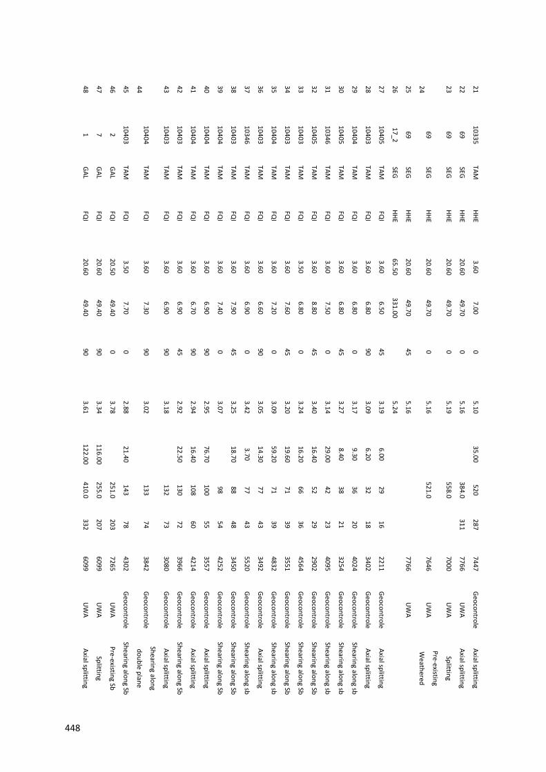
21 10335
TAM
HHE 3.60
7.00 0
5.10 35.00
520 287
7447 Geocontrole
Axial splitting
22 69
SEG HHE
20.60 49.70
0 5.16
384.0 311
7766 U
WA
Axial splitting
23 69
SEG HHE
20.60 49.70
0 5.19
558.0 7000
UW
A Splitting
24 69
SEG HHE
20.60 49.70
0 5.16
521.0 7646
UW
A Pre-existing
Weathered
25 69
SEG HHE
20.60 49.70
45 5.16
7766 U
WA
26 17_2
SEG HHE
65.50 331.00
5.24
27 10405
TAM
FQI
3.60 6.50
45 3.19
6.00 29
16 2211
Geocontrole Axial splitting
28 10403
TAM
FQI
3.60 6.80
90 3.09
6.20 32
18 3402
Geocontrole Axial splitting
29 10404
TAM
FQI
3.60 6.80
0 3.17
9.30 36
20 4024
Geocontrole Shearing along sb
30 10405
TAM
FQI
3.60 6.80
45 3.27
8.40 38
21 3254
Geocontrole Shearing along sb
31 10346
TAM
FQI
3.60 7.50
0 3.14
29.00 42
23 4095
Geocontrole Shearing along sb
32 10405
TAM
FQI
3.60 8.80
45 3.40
16.40 52
29 2902
Geocontrole Shearing along Sb
33 10403
TAM
FQI
3.50 6.80
0 3.24
16.20 66
36 4564
Geocontrole Shearing along Sb
34 10403
TAM
FQI
3.60 7.60
45 3.20
19.60 71
39 3551
Geocontrole Shearing along Sb
35 10404
TAM
FQI
3.60 7.20
0 3.09
59.20 71
39 4832
Geocontrole Shearing along sb
36 10403
TAM
FQI
3.60 6.60
90 3.05
14.30 77
43 3492
Geocontrole Axial splitting
37 10346
TAM
FQI
3.60 6.90
0 3.42
3.70 77
43 5520
Geocontrole Shearing along sb
38 10403
TAM
FQI
3.60 7.90
45 3.25
18.70 88
48 3450
Geocontrole Shearing along Sb
39 10404
TAM
FQI
3.60 7.40
0 3.07
98 54
4252 Geocontrole
Shearing along Sb
40 10404
TAM
FQI
3.60 6.90
90 2.95
76.70 100
55 3557
Geocontrole Axial splitting
41 10404
TAM
FQI
3.60 6.70
90 2.94
16.40 108
60 4214
Geocontrole Axial splitting
42 10403
TAM
FQI
3.60 6.90
45 2.92
22.50 130
72 3966
Geocontrole Shearing along Sb
43 10403
TAM
FQI
3.60 6.90
90 3.18
132 73
3080 Geocontrole
Axial splitting
44 10404
TAM
FQI
3.60 7.30
90 3.02
133 74
3842 Geocontrole
Shearing along
double plane
45 10403
TAM
FQI
3.50 7.70
0 2.88
21.40 143
78 4302
Geocontrole Shearing along Sb
46 2
GAL FQ
I 20.50
49.40 0
3.78 251.0
203 7265
UW
A Pre-existing Sb
47 7
GAL FQ
I 20.60
49.40 90
3.34 116.00
255.0 207
6099 U
WA
Splitting
48 1
GAL FQ
I 20.60
49.40 90
3.61 122.00
410.0 332
6099 U
WA
Axial splitting
448
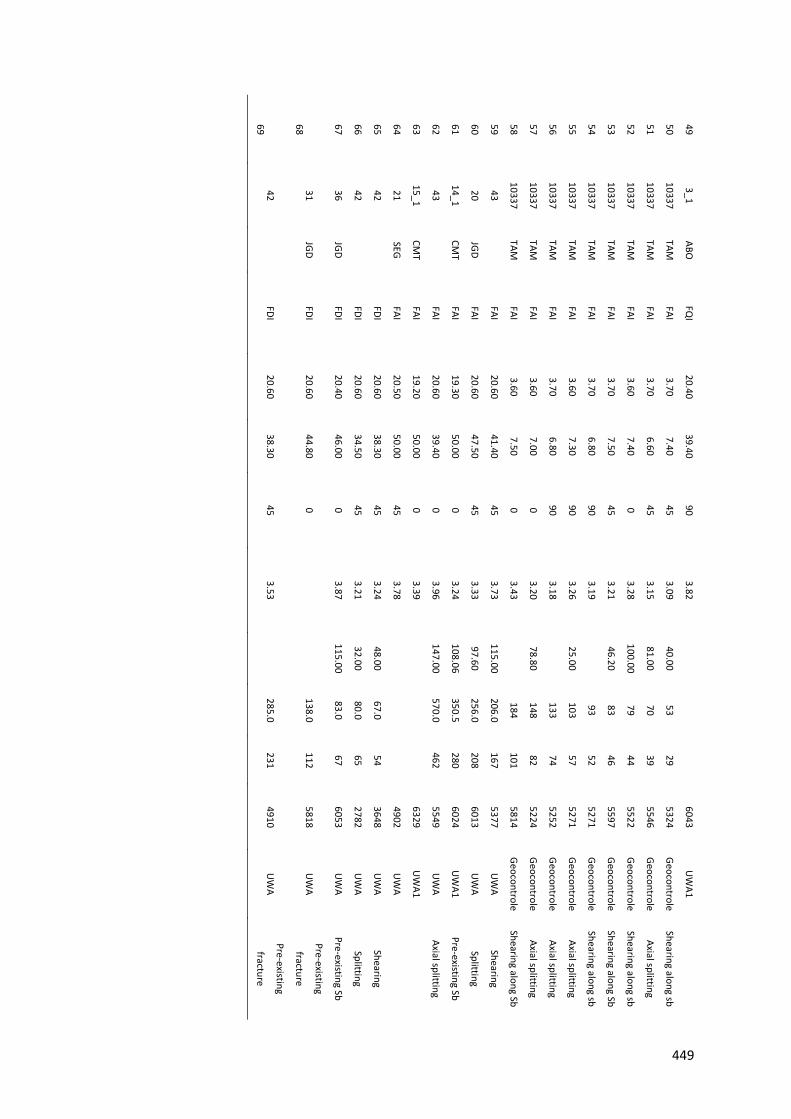
49 3_1
ABO
FQI
20.40 39.40
90 3.82
6043 U
WA1
50 10337
TAM
FAI 3.70
7.40 45
3.09 40.00
53 29
5324 Geocontrole
Shearing along sb
51 10337
TAM
FAI 3.70
6.60 45
3.15 81.00
70 39
5546 Geocontrole
Axial splitting
52 10337
TAM
FAI 3.60
7.40 0
3.28 100.00
79 44
5522 Geocontrole
Shearing along sb
53 10337
TAM
FAI 3.70
7.50 45
3.21 46.20
83 46
5597 Geocontrole
Shearing along Sb
54 10337
TAM
FAI 3.70
6.80 90
3.19 93
52 5271
Geocontrole Shearing along sb
55 10337
TAM
FAI 3.60
7.30 90
3.26 25.00
103 57
5271 Geocontrole
Axial splitting
56 10337
TAM
FAI 3.70
6.80 90
3.18 133
74 5252
Geocontrole Axial splitting
57 10337
TAM
FAI 3.60
7.00 0
3.20 78.80
148 82
5224 Geocontrole
Axial splitting
58 10337
TAM
FAI 3.60
7.50 0
3.43 184
101 5814
Geocontrole Shearing along Sb
59 43
FAI 20.60
41.40 45
3.73 115.00
206.0 167
5377 U
WA
Shearing
60 20
JGD FAI
20.60 47.50
45 3.33
97.60 256.0
208 6013
UW
A Splitting
61 14_1
CMT
FAI 19.30
50.00 0
3.24 108.06
350.5 280
6024 U
WA1
Pre-existing Sb
62 43
FAI 20.60
39.40 0
3.96 147.00
570.0 462
5549 U
WA
Axial splitting
63 15_1
CMT
FAI 19.20
50.00 0
3.39 6329
UW
A1
64 21
SEG FAI
20.50 50.00
45 3.78
4902 U
WA
65 42
FDI 20.60
38.30 45
3.24 48.00
67.0 54
3648 U
WA
Shearing
66 42
FDI 20.60
34.50 45
3.21 32.00
80.0 65
2782 U
WA
Splitting
67 36
JGD FDI
20.40 46.00
0 3.87
115.00 83.0
67 6053
UW
A Pre-existing Sb
68 31
JGD FDI
20.60 44.80
0 138.0
112 5818
UW
A Pre-existing
fracture
69 42
FDI 20.60
38.30 45
3.53 285.0
231 4910
UW
A Pre-existing
fracture
449

450
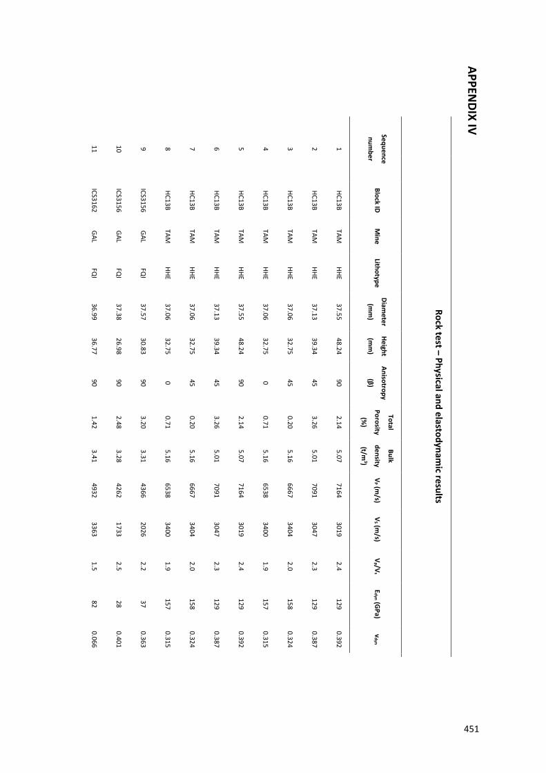
APPENDIX IV
Rock test – Physical and elastodynamic results
Sequence
number
Block ID M
ine Lithotype
Diameter
(mm
)
Height
(mm
)
Anisotropy
(β)
Total
Porosity
(%)
Bulk
density
(t/m3)
VP (m
/s) V
S (m/s)
Vp /V
s E
dyn (GPa)
vdyn
1 HC13B
TAM
HHE 37.55
48.24 90
2.14 5.07
7164 3019
2.4 129
0.392
2 HC13B
TAM
HHE 37.13
39.34 45
3.26 5.01
7091 3047
2.3 129
0.387
3 HC13B
TAM
HHE 37.06
32.75 45
0.20 5.16
6667 3404
2.0 158
0.324
4 HC13B
TAM
HHE 37.06
32.75 0
0.71 5.16
6538 3400
1.9 157
0.315
5 HC13B
TAM
HHE 37.55
48.24 90
2.14 5.07
7164 3019
2.4 129
0.392
6 HC13B
TAM
HHE 37.13
39.34 45
3.26 5.01
7091 3047
2.3 129
0.387
7 HC13B
TAM
HHE 37.06
32.75 45
0.20 5.16
6667 3404
2.0 158
0.324
8 HC13B
TAM
HHE 37.06
32.75 0
0.71 5.16
6538 3400
1.9 157
0.315
9 ICS3156
GAL FQ
I 37.57
30.83 90
3.20 3.31
4366 2026
2.2 37
0.363
10 ICS3156
GAL FQ
I 37.38
26.98 90
2.48 3.28
4262 1733
2.5 28
0.401
11 ICS3162
GAL FQ
I 36.99
36.77 90
1.42 3.41
4932 3363
1.5 82
0.066
451
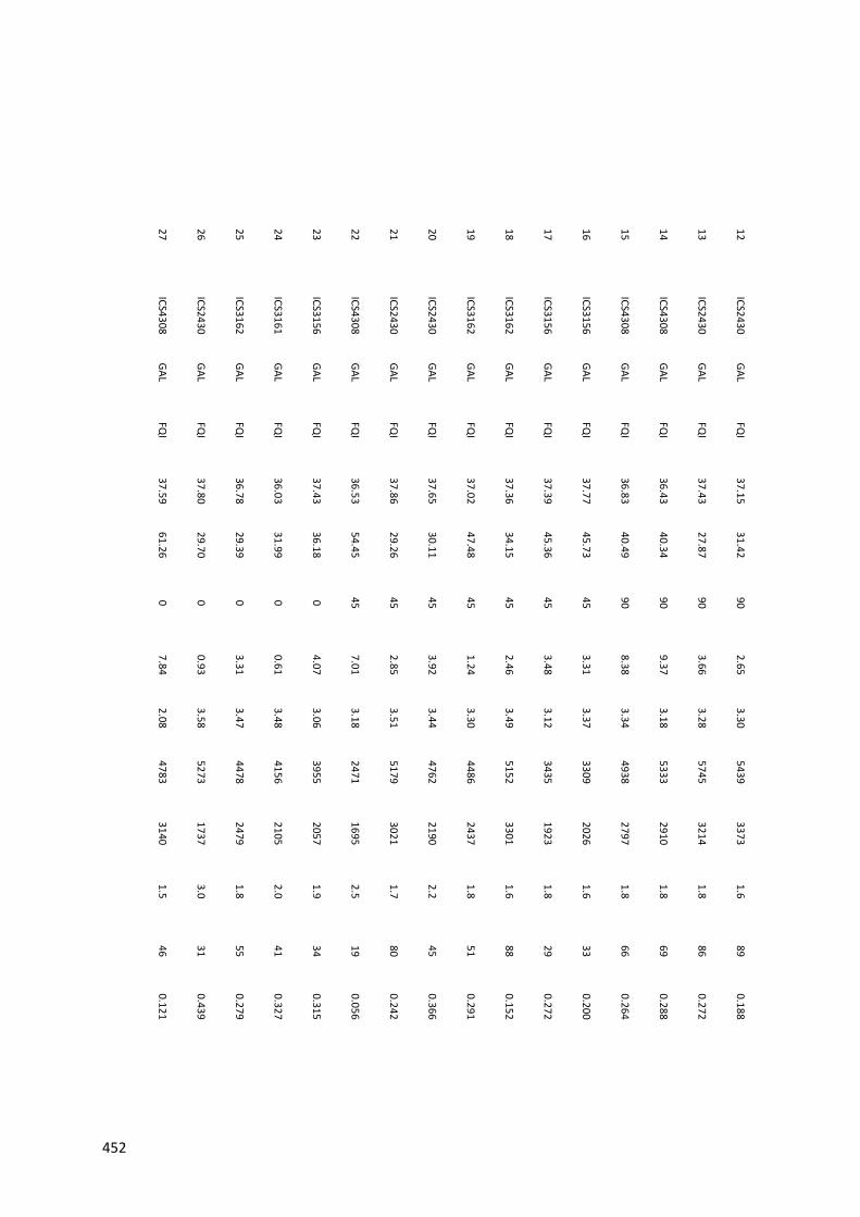
12 ICS2430
GAL FQ
I 37.15
31.42 90
2.65 3.30
5439 3373
1.6 89
0.188
13 ICS2430
GAL FQ
I 37.43
27.87 90
3.66 3.28
5745 3214
1.8 86
0.272
14 ICS4308
GAL FQ
I 36.43
40.34 90
9.37 3.18
5333 2910
1.8 69
0.288
15 ICS4308
GAL FQ
I 36.83
40.49 90
8.38 3.34
4938 2797
1.8 66
0.264
16 ICS3156
GAL FQ
I 37.77
45.73 45
3.31 3.37
3309 2026
1.6 33
0.200
17 ICS3156
GAL FQ
I 37.39
45.36 45
3.48 3.12
3435 1923
1.8 29
0.272
18 ICS3162
GAL FQ
I 37.36
34.15 45
2.46 3.49
5152 3301
1.6 88
0.152
19 ICS3162
GAL FQ
I 37.02
47.48 45
1.24 3.30
4486 2437
1.8 51
0.291
20 ICS2430
GAL FQ
I 37.65
30.11 45
3.92 3.44
4762 2190
2.2 45
0.366
21 ICS2430
GAL FQ
I 37.86
29.26 45
2.85 3.51
5179 3021
1.7 80
0.242
22 ICS4308
GAL FQ
I 36.53
54.45 45
7.01 3.18
2471 1695
2.5 19
0.056
23 ICS3156
GAL FQ
I 37.43
36.18 0
4.07 3.06
3955 2057
1.9 34
0.315
24 ICS3161
GAL FQ
I 36.03
31.99 0
0.61 3.48
4156 2105
2.0 41
0.327
25 ICS3162
GAL FQ
I 36.78
29.39 0
3.31 3.47
4478 2479
1.8 55
0.279
26 ICS2430
GAL FQ
I 37.80
29.70 0
0.93 3.58
5273 1737
3.0 31
0.439
27 ICS4308
GAL FQ
I 37.59
61.26 0
7.84 2.08
4783 3140
1.5 46
0.121
452
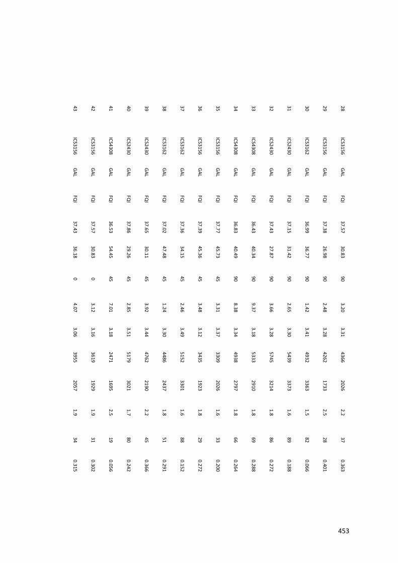
28 ICS3156
GAL FQ
I 37.57
30.83 90
3.20 3.31
4366 2026
2.2 37
0.363
29 ICS3156
GAL FQ
I 37.38
26.98 90
2.48 3.28
4262 1733
2.5 28
0.401
30 ICS3162
GAL FQ
I 36.99
36.77 90
1.42 3.41
4932 3363
1.5 82
0.066
31 ICS2430
GAL FQ
I 37.15
31.42 90
2.65 3.30
5439 3373
1.6 89
0.188
32 ICS2430
GAL FQ
I 37.43
27.87 90
3.66 3.28
5745 3214
1.8 86
0.272
33 ICS4308
GAL FQ
I 36.43
40.34 90
9.37 3.18
5333 2910
1.8 69
0.288
34 ICS4308
GAL FQ
I 36.83
40.49 90
8.38 3.34
4938 2797
1.8 66
0.264
35 ICS3156
GAL FQ
I 37.77
45.73 45
3.31 3.37
3309 2026
1.6 33
0.200
36 ICS3156
GAL FQ
I 37.39
45.36 45
3.48 3.12
3435 1923
1.8 29
0.272
37 ICS3162
GAL FQ
I 37.36
34.15 45
2.46 3.49
5152 3301
1.6 88
0.152
38 ICS3162
GAL FQ
I 37.02
47.48 45
1.24 3.30
4486 2437
1.8 51
0.291
39 ICS2430
GAL FQ
I 37.65
30.11 45
3.92 3.44
4762 2190
2.2 45
0.366
40 ICS2430
GAL FQ
I 37.86
29.26 45
2.85 3.51
5179 3021
1.7 80
0.242
41 ICS4308
GAL FQ
I 36.53
54.45 45
7.01 3.18
2471 1695
2.5 19
0.056
42 ICS3156
GAL FQ
I 37.57
30.83 0
3.12 3.16
3619 1929
1.9 31
0.302
43 ICS3156
GAL FQ
I 37.43
36.18 0
4.07 3.06
3955 2057
1.9 34
0.315
453
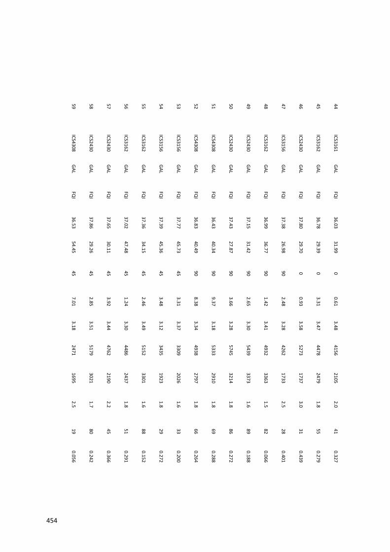
44 ICS3161
GAL FQ
I 36.03
31.99 0
0.61 3.48
4156 2105
2.0 41
0.327
45 ICS3162
GAL FQ
I 36.78
29.39 0
3.31 3.47
4478 2479
1.8 55
0.279
46 ICS2430
GAL FQ
I 37.80
29.70 0
0.93 3.58
5273 1737
3.0 31
0.439
47 ICS3156
GAL FQ
I 37.38
26.98 90
2.48 3.28
4262 1733
2.5 28
0.401
48 ICS3162
GAL FQ
I 36.99
36.77 90
1.42 3.41
4932 3363
1.5 82
0.066
49 ICS2430
GAL FQ
I 37.15
31.42 90
2.65 3.30
5439 3373
1.6 89
0.188
50 ICS2430
GAL FQ
I 37.43
27.87 90
3.66 3.28
5745 3214
1.8 86
0.272
51 ICS4308
GAL FQ
I 36.43
40.34 90
9.37 3.18
5333 2910
1.8 69
0.288
52 ICS4308
GAL FQ
I 36.83
40.49 90
8.38 3.34
4938 2797
1.8 66
0.264
53 ICS3156
GAL FQ
I 37.77
45.73 45
3.31 3.37
3309 2026
1.6 33
0.200
54 ICS3156
GAL FQ
I 37.39
45.36 45
3.48 3.12
3435 1923
1.8 29
0.272
55 ICS3162
GAL FQ
I 37.36
34.15 45
2.46 3.49
5152 3301
1.6 88
0.152
56 ICS3162
GAL FQ
I 37.02
47.48 45
1.24 3.30
4486 2437
1.8 51
0.291
57 ICS2430
GAL FQ
I 37.65
30.11 45
3.92 3.44
4762 2190
2.2 45
0.366
58 ICS2430
GAL FQ
I 37.86
29.26 45
2.85 3.51
5179 3021
1.7 80
0.242
59 ICS4308
GAL FQ
I 36.53
54.45 45
7.01 3.18
2471 1695
2.5 19
0.056
454
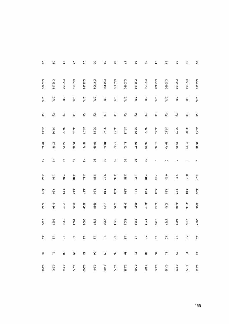
60 ICS3156
GAL FQ
I 37.43
36.18 0
4.07 3.06
3955 2057
1.9 34
0.315
61 ICS3161
GAL FQ
I 36.03
31.99 0
0.61 3.48
4156 2105
2.0 41
0.327
62 ICS3162
GAL FQ
I 36.78
29.39 0
3.31 3.47
4478 2479
1.8 55
0.279
63 ICS2430
GAL FQ
I 37.80
29.70 0
0.93 3.58
5273 1737
3.0 31
0.439
64 ICS4308
GAL FQ
I 37.59
61.26 0
7.84 2.08
4783 3140
1.5 46
0.121
65 ICS3156
GAL FQ
I 37.38
26.98 90
2.48 3.28
4262 1733
2.5 28
0.401
66 ICS3162
GAL FQ
I 36.99
36.77 90
1.42 3.41
4932 3363
1.5 82
0.066
67 ICS2430
GAL FQ
I 37.15
31.42 90
2.65 3.30
5439 3373
1.6 89
0.188
68 ICS2430
GAL FQ
I 37.43
27.87 90
3.66 3.28
5745 3214
1.8 86
0.272
69 ICS4308
GAL FQ
I 36.43
40.34 90
9.37 3.18
5333 2910
1.8 69
0.288
70 ICS4308
GAL FQ
I 36.83
40.49 90
8.38 3.34
4938 2797
1.8 66
0.264
71 ICS3156
GAL FQ
I 37.77
45.73 45
3.31 3.37
3309 2026
1.6 33
0.200
72 ICS3156
GAL FQ
I 37.39
45.36 45
3.48 3.12
3435 1923
1.8 29
0.272
73 ICS3162
GAL FQ
I 37.36
34.15 45
2.46 3.49
5152 3301
1.6 88
0.152
74 ICS3162
GAL FQ
I 37.02
47.48 45
1.24 3.30
4486 2437
1.8 51
0.291
75 ICS2430
GAL FQ
I 37.65
30.11 45
3.92 3.44
4762 2190
2.2 45
0.366
455
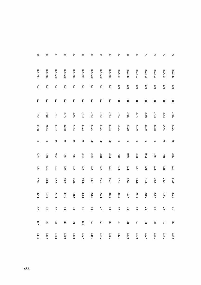
76 ICS2430
GAL FQ
I 37.86
29.26 45
2.85 3.51
5179 3021
1.7 80
0.242
77 ICS4308
GAL FQ
I 36.53
54.45 45
7.01 3.18
2471 1695
2.5 19
0.056
78 ICS3156
GAL FQ
I 37.43
36.18 0
4.07 3.06
3955 2057
1.9 34
0.315
79 ICS3161
GAL FQ
I 36.03
31.99 0
0.61 3.48
4156 2105
2.0 41
0.327
80 ICS3162
GAL FQ
I 36.78
29.39 0
3.31 3.47
4478 2479
1.8 55
0.279
81 ICS2430
GAL FQ
I 37.80
29.70 0
0.93 3.58
5273 1737
3.0 31
0.439
82 ICS4308
GAL FQ
I 37.59
61.26 0
7.84 2.08
4783 3140
1.5 46
0.121
83 ICA3244
SAP FAI
37.58 35.93
90 3.51
3.24 5537
3130 1.8
80 0.265
84 ICA3620
SAP FAI
37.57 33.75
90 3.81
3.25 5593
2724 2.1
65 0.345
85 ICA3620
SAP FAI
37.57 33.75
90 2.23
3.25 4457
2781 1.6
59 0.181
86 ICA3244
SAP FAI
37.42 45.73
45 3.42
3.35 5998
3563 1.7
104 0.227
87 ICA3244
SAP FAI
36.95 28.14
45 7.07
3.25 4516
1482 3.0
21 0.440
88 ICA3620
SAP FAI
35.75 37.50
45 1.90
3.49 5069
3076 1.6
80 0.209
89 ICA3620
SAP FAI
37.10 39.82
45 9.52
3.24 4255
2273 1.9
44 0.300
90 ICA3244
SAP FAI
37.87 24.14
0 1.94
3.54 4898
1579 3.1
25 0.442
91 ICA3243
SAP FAI
37.52 36.18
0 5.22
3.43 5713
3714 1.5
107 0.134
456
92 ICA3620
SAP FAI
36.56 59.53
0 1.19
3.39 5172
3452 1.3
89 0.098
93 ICA3620
SAP FAI
37.36 40.58
0 5.33
3.38 5195
3276 1.6
85 0.170
94 ICA3244
SAP FAI
37.58 35.93
90 3.51
3.24 5537
3130 1.8
80 0.265
95 ICA3620
SAP FAI
37.57 33.75
90 3.81
3.25 5593
2724 2.1
65 0.345
96 ICA3620
SAP FAI
37.57 33.75
90 2.23
3.25 4457
2781 1.6
59 0.181
97 ICA3244
SAP FAI
37.42 45.73
45 3.42
3.35 5998
3563 1.7
104 0.227
98 ICA3244
SAP FAI
36.95 28.14
45 7.07
3.25 4516
1482 3.0
21 0.440
99 ICA3620
SAP FAI
35.75 37.50
45 1.90
3.49 5069
3076 1.6
80 0.209
100 ICA3620
SAP FAI
37.10 39.82
45 9.52
3.24 4255
2273 1.9
44 0.300
101 ICA3244
SAP FAI
37.87 24.14
0 1.94
3.54 4898
1579 3.1
25 0.442
102 ICA3243
SAP FAI
37.52 36.18
0 5.22
3.43 5713
3714 1.5
107 0.134
103 ICA3620
SAP FAI
36.56 59.53
0 1.19
3.39 5172
3452 1.3
89 0.098
104 ICA3620
SAP FAI
37.36 40.58
0 5.33
3.38 5195
3276 1.6
85 0.170
105 ICA3244
SAP FAI
37.58 35.93
90 3.51
3.24 5537
3130 1.8
80 0.265
106 ICA3620
SAP FAI
37.57 33.75
90 3.81
3.25 5593
2724 2.1
65 0.345
107 ICA3620
SAP FAI
37.57 33.75
90 2.23
3.25 4457
2781 1.6
59 0.181
457
108 ICA3244
SAP FAI
37.42 45.73
45 3.42
3.35 5998
3563 1.7
104 0.227
109 ICA3244
SAP FAI
36.95 28.14
45 7.07
3.25 4516
1482 3.0
21 0.440
110 ICA3620
SAP FAI
35.75 37.50
45 1.90
3.49 5069
3076 1.6
80 0.209
111 ICA3620
SAP FAI
37.10 39.82
45 9.52
3.24 4255
2273 1.9
44 0.300
112 ICA3244
SAP FAI
37.87 24.14
0 1.94
3.54 4898
1579 3.1
25 0.442
113 ICA3243
SAP FAI
37.52 36.18
0 5.22
3.43 5713
3714 1.5
107 0.134
114 ICA3620
SAP FAI
36.56 59.53
0 1.19
3.39 5172
3452 1.3
89 0.098
115 ICA3620
SAP FAI
37.36 40.58
0 5.33
3.38 5195
3276 1.6
85 0.170
116 ICA3244
SAP FAI
37.58 35.93
90 3.51
3.24 5537
3130 1.8
80 0.265
117 ICA3620
SAP FAI
37.57 33.75
90 3.81
3.25 5593
2724 2.1
65 0.345
118 ICA3620
SAP FAI
37.57 33.75
90 2.23
3.25 4457
2781 1.6
59 0.181
119 ICA3244
SAP FAI
37.42 45.73
45 3.42
3.35 5998
3563 1.7
104 0.227
120 ICA3244
SAP FAI
36.95 28.14
45 7.07
3.25 4516
1482 3.0
21 0.440
121 ICA3620
SAP FAI
35.75 37.50
45 1.90
3.49 5069
3076 1.6
80 0.209
122 ICA3620
SAP FAI
37.10 39.82
45 9.52
3.24 4255
2273 1.9
44 0.300
123 ICA3244
SAP FAI
37.87 24.14
0 1.94
3.54 4898
1579 3.1
25 0.442
458
124 ICA3243
SAP FAI
37.52 36.18
0 5.22
3.43 5713
3714 1.5
107 0.134
125 ICA3620
SAP FAI
36.56 59.53
0 1.19
3.39 5172
3452 1.3
89 0.098
126 ICA3620
SAP FAI
37.36 40.58
0 5.33
3.38 5195
3276 1.6
85 0.170
127 ID2402
CPX FDI
37.97 31.07
90 2.89
3.38 5082
1856 2.7
33 0.423
128 ID2402
CPX FDI
37.87 25.54
90 4.68
3.01 5108
2453 2.1
49 0.350
129 ID2402
CPX FDI
38.01 28.67
90 2.91
3.48 5088
2871 1.8
73 0.266
130 ID1780
CPX FDI
37.70 42.30
90 0.49
2.56 6364
3621 1.8
85 0.261
131 ID1780
CPX FDI
37.70 40.60
90 0.77
3.27 5857
2611 2.2
61 0.376
132 ID3294
CPX FDI
38.03 36.93
90 1.04
2.85 4867
2569 1.9
49 0.307
133 ID3294
CPX FDI
38.21 41.30
90 3.33
2.78 6212
2993 2.1
67 0.349
134 ID3202
CPX FDI
37.59 51.34
90 2.37
3.43 5667
2833 2.0
73 0.333
135 ID3284
CPX FDI
37.21 28.43
90 1.38
3.71 4375
2074 2.1
43 0.355
136 ID2212
CPX FDI
37.80 49.50
45 0.99
2.96 6494
3030 2.1
74 0.361
137 ID2402
CPX FDI
37.47 57.20
45 2.58
3.02 4524
3115 1.5
61 0.049
138 ID1780
CPX FDI
3.77 48.80
45 0.66
2.30 5568
2367 2.4
36 0.390
139 ID3294
CPX FDI
37.22 39.57
45 1.40
2.84 5909
3611 1.6
89 0.202
459
140 ID3294
CPX FDI
38.16 37.04
45 2.98
2.77 5966
2215 2.7
39 0.420
141 ID3202
CPX FDI
37.39 57.14
45 2.94
3.82 5429
2676 2.0
73 0.340
142 ID3202
CPX FDI
37.98 50.56
45 1.07
3.67 5952
3311 1.8
103 0.276
143 ID3284
CPX FDI
37.15 36.66
45 3.79
3.55 4457
3007 1.5
69 0.082
144 ID2212
CPX FDI
37.73 39.78
0 2.99
2.53 4444
2920 1.5
48 0.120
145 ID2401
CPX FDI
37.63 32.60
0 3.94
3.55 5156
2870 1.8
75 0.276
146 ID2402
CPX FDI
37.12 22.55
0 2.32
3.41 5227
1825 2.9
32 0.431
147 ID17780
CPX FDI
37.70 51.40
0 0.09
2.41 5102
2795 1.8
48 0.286
148 ID3294
CPX FDI
37.88 24.83
0 3.11
2.80 6944
3425 2.0
88 0.339
149 ID3294
CPX FDI
38.11 29.56
0 3.71
2.84 5472
2417 2.3
46 0.379
150 ID3202
CPX FDI
37.90 42.88
0 2.20
3.51 5316
2500 2.1
60 0.358
151 ID3202
CPX FDI
37.42 29.70
0 2.10
3.68 4545
2086 2.2
44 0.367
152 ID3284
CPX FDI
37.50 35.80
0 1.63
3.52 4545
2397 1.9
53 0.307
153 ID2402
CPX FDI
37.97 31.07
90 2.89
3.38 5082
1856 2.7
33 0.423
154 ID2402
CPX FDI
37.87 25.54
90 4.68
3.01 5108
2453 2.1
49 0.350
155 ID2402
CPX FDI
38.01 28.67
90 2.91
3.48 5088
2871 1.8
73 0.266
460
156 ID1780
CPX FDI
37.70 42.30
90 0.49
2.56 6364
3621 1.8
85 0.261
157 ID1780
CPX FDI
37.70 40.60
90 0.77
3.27 5857
2611 2.2
61 0.376
158 ID3294
CPX FDI
38.03 36.93
90 1.04
2.85 4867
2569 1.9
49 0.307
159 ID3294
CPX FDI
38.21 41.30
90 3.33
2.78 6212
2993 2.1
67 0.349
160 ID3202
CPX FDI
37.59 51.34
90 2.37
3.43 5667
2833 2.0
73 0.333
161 ID3284
CPX FDI
37.21 28.43
90 1.38
3.71 4375
2074 2.1
43 0.355
162 ID2212
CPX FDI
37.80 49.50
45 0.99
2.96 6494
3030 2.1
74 0.361
163 ID2402
CPX FDI
37.47 57.20
45 2.58
3.02 4524
3115 1.5
61 0.049
164 ID1780
CPX FDI
3.77 48.80
45 0.66
2.30 5568
2367 2.4
36 0.390
165 ID3294
CPX FDI
37.22 39.57
45 1.40
2.84 5909
3611 1.6
89 0.202
166 ID3294
CPX FDI
38.16 37.04
45 2.98
2.77 5966
2215 2.7
39 0.420
167 ID3202
CPX FDI
37.39 57.14
45 2.94
3.82 5429
2676 2.0
73 0.340
168 ID3202
CPX FDI
37.98 50.56
45 1.07
3.67 5952
3311 1.8
103 0.276
169 ID3284
CPX FDI
37.15 36.66
45 3.79
3.55 4457
3007 1.5
69 0.082
170 ID2212
CPX FDI
37.73 39.78
0 2.99
2.53 4444
2920 1.5
48 0.120
171 ID2401
CPX FDI
37.63 32.60
0 3.94
3.55 5156
2870 1.8
75 0.276
461
172 ID2402
CPX FDI
37.12 22.55
0 2.32
3.41 5227
1825 2.9
32 0.431
173 ID17780
CPX FDI
37.70 51.40
0 0.09
2.41 5102
2795 1.8
48 0.286
174 ID3294
CPX FDI
37.88 24.83
0 3.11
2.80 6944
3425 2.0
88 0.339
175 ID3294
CPX FDI
38.11 29.56
0 3.71
2.84 5472
2417 2.3
46 0.379
176 ID3202
CPX FDI
37.90 42.88
0 2.20
3.51 5316
2500 2.1
60 0.358
177 ID3202
CPX FDI
37.42 29.70
0 2.10
3.68 4545
2086 2.2
44 0.367
178 ID3284
CPX FDI
37.50 35.80
0 1.63
3.52 4545
2397 1.9
53 0.307
179 ID2402
CPX FDI
37.97 31.07
90 2.89
3.38 5082
1856 2.7
33 0.423
180 ID2402
CPX FDI
37.87 25.54
90 4.68
3.01 5108
2453 2.1
49 0.350
181 ID2402
CPX FDI
38.01 28.67
90 2.91
3.48 5088
2871 1.8
73 0.266
182 ID1780
CPX FDI
37.70 42.30
90 0.49
2.56 6364
3621 1.8
85 0.261
183 ID1780
CPX FDI
37.70 40.60
90 0.77
3.27 5857
2611 2.2
61 0.376
184 ID3294
CPX FDI
38.03 36.93
90 1.04
2.85 4867
2569 1.9
49 0.307
185 ID3294
CPX FDI
38.21 41.30
90 3.33
2.78 6212
2993 2.1
67 0.349
186 ID3202
CPX FDI
37.59 51.34
90 2.37
3.43 5667
2833 2.0
73 0.333
187 ID3284
CPX FDI
37.21 28.43
90 1.38
3.71 4375
2074 2.1
43 0.355
462
188 ID2212
CPX FDI
37.80 49.50
45 0.99
2.96 6494
3030 2.1
74 0.361
189 ID2402
CPX FDI
37.47 57.20
45 2.58
3.02 4524
3115 1.5
61 0.049
190 ID1780
CPX FDI
3.77 48.80
45 0.66
2.30 5568
2367 2.4
36 0.390
191 ID3294
CPX FDI
37.22 39.57
45 1.40
2.84 5909
3611 1.6
89 0.202
192 ID3294
CPX FDI
38.16 37.04
45 2.98
2.77 5966
2215 2.7
39 0.420
193 ID3202
CPX FDI
37.39 57.14
45 2.94
3.82 5429
2676 2.0
73 0.340
194 ID3202
CPX FDI
37.98 50.56
45 1.07
3.67 5952
3311 1.8
103 0.276
195 ID3284
CPX FDI
37.15 36.66
45 3.79
3.55 4457
3007 1.5
69 0.082
196 ID2212
CPX FDI
37.73 39.78
0 2.99
2.53 4444
2920 1.5
48 0.120
197 ID2401
CPX FDI
37.63 32.60
0 3.94
3.55 5156
2870 1.8
75 0.276
198 ID2402
CPX FDI
37.12 22.55
0 2.32
3.41 5227
1825 2.9
32 0.431
199 ID17780
CPX FDI
37.70 51.40
0 0.09
2.41 5102
2795 1.8
48 0.286
200 ID3294
CPX FDI
37.88 24.83
0 3.11
2.80 6944
3425 2.0
88 0.339
201 ID3294
CPX FDI
38.11 29.56
0 3.71
2.84 5472
2417 2.3
46 0.379
202 ID3202
CPX FDI
37.90 42.88
0 2.20
3.51 5316
2500 2.1
60 0.358
203 ID3202
CPX FDI
37.42 29.70
0 2.10
3.68 4545
2086 2.2
44 0.367
463
204 ID3284
CPX FDI
37.50 35.80
0 1.63
3.52 4545
2397 1.9
53 0.307
205 IM
S2348 GAL
PWQ
I 37.70
53.70 90
26.42 2.92
2978 1398
2.1 16
0.359
206 IM
S2348 GAL
PWQ
I 37.60
49.30 90
26.30 2.92
2818 1056
2.7 9
0.418
207 IM
S2348 GAL
PWQ
I 37.70
53.40 90
27.30 2.81
2733 1274
2.1 12
0.361
208 IM
S2348 GAL
PWQ
I 37.60
29.20 90
22.32 2.47
2377 1213
2.0 10
0.324
209 IM
S2348 GAL
PWQ
I 37.50
26.90 90
27.38 2.86
2766 1238
2.2 12
0.375
210 IM
S2348 GAL
PWQ
I 37.70
45.20 0
29.99 2.79
2242 1327
1.7 12
0.230
211 IM
S2348 GAL
PWQ
I 37.70
43.20 0
25.97 2.94
2099 1269
1.7 11
0.212
212 IM
S2348 GAL
PWQ
I 37.70
53.70 90
26.42 2.92
2978 1398
2.1 16
0.359
213 IM
S2348 GAL
PWQ
I 37.60
49.30 90
26.30 2.92
2818 1056
2.7 9
0.418
214 IM
S2348 GAL
PWQ
I 37.70
53.40 90
27.30 2.81
2733 1274
2.1 12
0.361
215 IM
S2348 GAL
PWQ
I 37.60
29.20 90
22.32 2.47
2377 1213
2.0 10
0.324
216 IM
S2348 GAL
PWQ
I 37.50
26.90 90
27.38 2.86
2766 1238
2.2 12
0.375
217 IM
S2348 GAL
PWQ
I 37.70
45.20 0
29.99 2.79
2242 1327
1.7 12
0.230
218 IM
S2348 GAL
PWQ
I 37.70
43.20 0
25.97 2.94
2099 1269
1.7 11
0.212
219 IM
S2348 GAL
PWQ
I 37.70
53.70 90
26.42 2.92
2978 1398
2.1 16
0.359
464
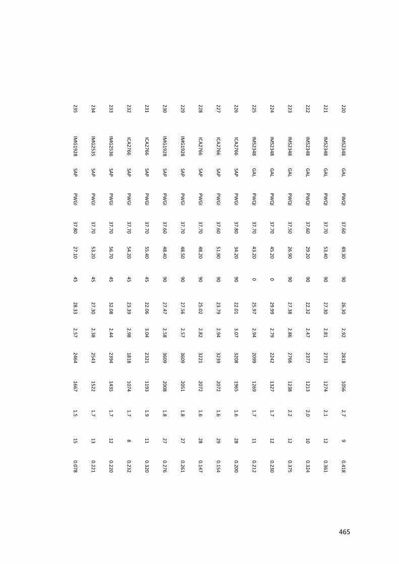
220 IM
S2348 GAL
PWQ
I 37.60
49.30 90
26.30 2.92
2818 1056
2.7 9
0.418
221 IM
S2348 GAL
PWQ
I 37.70
53.40 90
27.30 2.81
2733 1274
2.1 12
0.361
222 IM
S2348 GAL
PWQ
I 37.60
29.20 90
22.32 2.47
2377 1213
2.0 10
0.324
223 IM
S2348 GAL
PWQ
I 37.50
26.90 90
27.38 2.86
2766 1238
2.2 12
0.375
224 IM
S2348 GAL
PWQ
I 37.70
45.20 0
29.99 2.79
2242 1327
1.7 12
0.230
225 IM
S2348 GAL
PWQ
I 37.70
43.20 0
25.97 2.94
2099 1269
1.7 11
0.212
226 ICA2766
SAP PW
GI 37.80
34.20 90
22.01 3.07
3208 1965
1.6 28
0.200
227 ICA2766
SAP PW
GI 37.60
51.90 90
23.79 2.94
3239 2072
1.6 29
0.154
228 ICA2766
SAP PW
GI 37.70
48.20 90
25.02 2.82
3221 2072
1.6 28
0.147
229 IM
G1928 SAP
PWGI
37.70 48.50
90 27.56
2.57 3609
2051 1.8
27 0.261
230 IM
G1928 SAP
PWGI
37.60 48.40
90 27.47
2.58 3609
2008 1.8
27 0.276
231 ICA2766
SAP PW
GI 37.70
55.40 45
22.06 3.04
2321 1193
1.9 11
0.320
232 ICA2766
SAP PW
GI 37.70
54.20 45
23.39 2.98
1818 1074
1.7 8
0.232
233 IM
G2536 SAP
PWGI
37.70 56.70
45 32.08
2.44 2394
1435 1.7
12 0.220
234 IM
G2535 SAP
PWGI
37.70 53.20
45 27.30
2.38 2543
1522 1.7
13 0.221
235 IM
G1928 SAP
PWGI
37.80 27.10
45 28.33
2.57 2464
1667 1.5
15 0.078
465
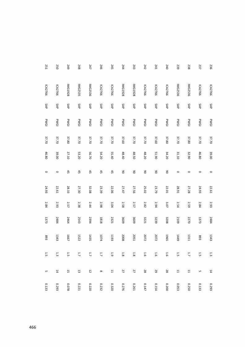
236 ICA2766
SAP PW
GI 37.70
39.00 0
22.61 2.93
2484 1343
1.3 14
0.293
237 ICA2766
SAP PW
GI 37.70
46.80 0
24.93 2.84
1373 893
1.5 5
0.133
238 IM
G2536 SAP
PWGI
37.80 32.90
0 27.28
2.59 2270
1311 1.7
11 0.250
239 IM
G2536 SAP
PWGI
37.70 31.10
0 28.91
2.54 2109
1449 1.5
11 0.053
240 ICA2766
SAP PW
GI 37.80
34.20 90
22.01 3.07
3208 1965
1.6 28
0.200
241 ICA2766
SAP PW
GI 37.60
51.90 90
23.79 2.94
3239 2072
1.6 29
0.154
242 ICA2766
SAP PW
GI 37.70
48.20 90
25.02 2.82
3221 2072
1.6 28
0.147
243 IM
G1928 SAP
PWGI
37.70 48.50
90 27.56
2.57 3609
2051 1.8
27 0.261
244 IM
G1928 SAP
PWGI
37.60 48.40
90 27.47
2.58 3609
2008 1.8
27 0.276
245 ICA2766
SAP PW
GI 37.70
55.40 45
22.06 3.04
2321 1193
1.9 11
0.320
246 ICA2766
SAP PW
GI 37.70
54.20 45
23.39 2.98
1818 1074
1.7 8
0.232
247 IM
G2536 SAP
PWGI
37.70 56.70
45 32.08
2.44 2394
1435 1.7
12 0.220
248 IM
G2535 SAP
PWGI
37.70 53.20
45 27.30
2.38 2543
1522 1.7
13 0.221
249 IM
G1928 SAP
PWGI
37.80 27.10
45 28.33
2.57 2464
1667 1.5
15 0.078
250 ICA2766
SAP PW
GI 37.70
39.00 0
22.61 2.93
2484 1343
1.3 14
0.293
251 ICA2766
SAP PW
GI 37.70
46.80 0
24.93 2.84
1373 893
1.5 5
0.133
466
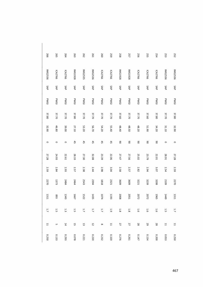
252 IM
G2536 SAP
PWGI
37.80 32.90
0 27.28
2.59 2270
1311 1.7
11 0.250
253 IM
G2536 SAP
PWGI
37.70 31.10
0 28.91
2.54 2109
1449 1.5
11 0.053
254 ICA2766
SAP PW
GI 37.80
34.20 90
22.01 3.07
3208 1965
1.6 28
0.200
255 ICA2766
SAP PW
GI 37.60
51.90 90
23.79 2.94
3239 2072
1.6 29
0.154
256 ICA2766
SAP PW
GI 37.70
48.20 90
25.02 2.82
3221 2072
1.6 28
0.147
257 IM
G1928 SAP
PWGI
37.70 48.50
90 27.56
2.57 3609
2051 1.8
27 0.261
258 IM
G1928 SAP
PWGI
37.60 48.40
90 27.47
2.58 3609
2008 1.8
27 0.276
259 ICA2766
SAP PW
GI 37.70
55.40 45
22.06 3.04
2321 1193
1.9 11
0.320
260 ICA2766
SAP PW
GI 37.70
54.20 45
23.39 2.98
1818 1074
1.7 8
0.232
261 IM
G2536 SAP
PWGI
37.70 56.70
45 32.08
2.44 2394
1435 1.7
12 0.220
262 IM
G2535 SAP
PWGI
37.70 53.20
45 27.30
2.38 2543
1522 1.7
13 0.221
263 IM
G1928 SAP
PWGI
37.80 27.10
45 28.33
2.57 2464
1667 1.5
15 0.078
264 ICA2766
SAP PW
GI 37.70
39.00 0
22.61 2.93
2484 1343
1.3 14
0.293
265 ICA2766
SAP PW
GI 37.70
46.80 0
24.93 2.84
1373 893
1.5 5
0.133
266 IM
G2536 SAP
PWGI
37.80 32.90
0 27.28
2.59 2270
1311 1.7
11 0.250
467

468
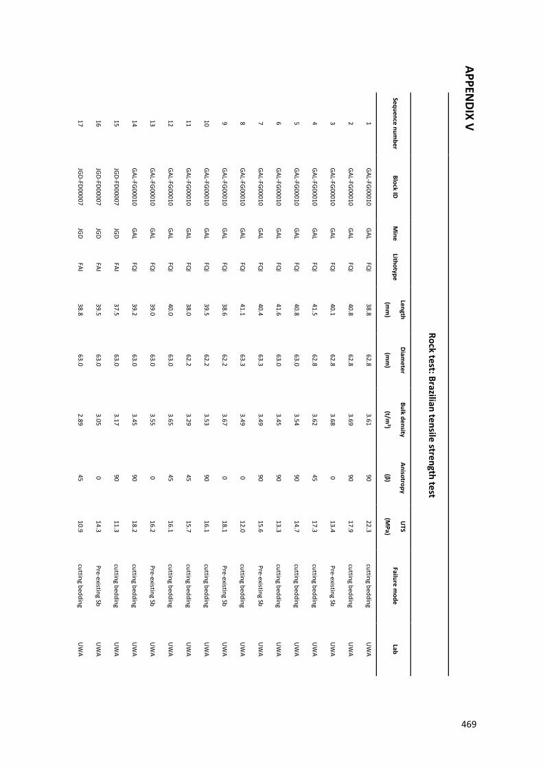
APPENDIX V
Rock test: Brazilian tensile strength test
Sequence number
Block ID
Mine
Lithotype Length
(mm
)
Diameter
(mm
)
Bulk density
(t/m3)
Anisotropy
(β)
UTS
(MPa)
Failure mode
Lab
1 G
AL-FG00010 G
AL FQ
I 38.8
62.8 3.61
90 22.3
cutting bedding U
WA
2 G
AL-FG00010 G
AL FQ
I 40.8
62.8 3.69
90 17.9
cutting bedding U
WA
3 G
AL-FG00010 G
AL FQ
I 40.1
62.8 3.68
0 13.4
Pre-existing Sb U
WA
4 G
AL-FG00010 G
AL FQ
I 41.5
62.8 3.62
45 17.3
cutting bedding U
WA
5 G
AL-FG00010 G
AL FQ
I 40.8
63.0 3.54
90 14.7
cutting bedding U
WA
6 G
AL-FG00010 G
AL FQ
I 41.6
63.0 3.45
90 13.3
cutting bedding U
WA
7 G
AL-FG00010 G
AL FQ
I 40.4
63.3 3.49
90 15.6
Pre-existing Sb U
WA
8 G
AL-FG00010 G
AL FQ
I 41.1
63.3 3.49
0 12.0
cutting bedding U
WA
9 G
AL-FG00010 G
AL FQ
I 38.6
62.2 3.67
0 18.1
Pre-existing Sb U
WA
10 G
AL-FG00010 G
AL FQ
I 39.5
62.2 3.53
90 16.1
cutting bedding U
WA
11 G
AL-FG00010 G
AL FQ
I 38.0
62.2 3.29
45 15.7
cutting bedding U
WA
12 G
AL-FG00010 G
AL FQ
I 40.0
63.0 3.65
45 16.1
cutting bedding U
WA
13 G
AL-FG00010 G
AL FQ
I 39.0
63.0 3.55
0 16.2
Pre-existing Sb U
WA
14 G
AL-FG00010 G
AL FQ
I 39.2
63.0 3.45
90 18.2
cutting bedding U
WA
15 JG
D-FD00007 JGD
FAI 37.5
63.0 3.17
90 11.3
cutting bedding U
WA
16 JG
D-FD00007 JGD
FAI 39.5
63.0 3.05
0 14.3
Pre-existing Sb U
WA
17 JG
D-FD00007 JGD
FAI 38.8
63.0 2.89
45 10.9
cutting bedding U
WA
469
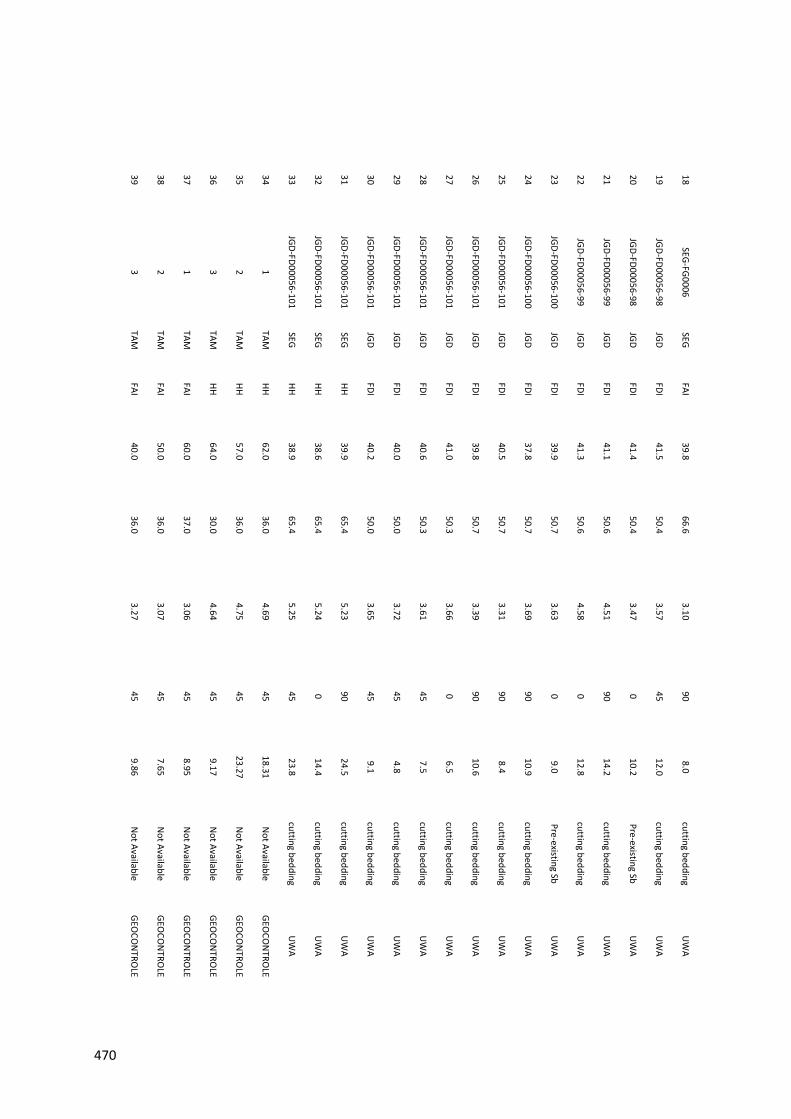
18 SEG-FG0006
SEG FAI
39.8 66.6
3.10 90
8.0 cutting bedding
UW
A
19 JGD-FD00056-98
JGD FDI
41.5 50.4
3.57 45
12.0 cutting bedding
UW
A
20 JGD-FD00056-98
JGD FDI
41.4 50.4
3.47 0
10.2 Pre-existing Sb
UW
A
21 JGD-FD00056-99
JGD FDI
41.1 50.6
4.51 90
14.2 cutting bedding
UW
A
22 JGD-FD00056-99
JGD FDI
41.3 50.6
4.58 0
12.8 cutting bedding
UW
A
23 JGD-FD00056-100
JGD FDI
39.9 50.7
3.63 0
9.0 Pre-existing Sb
UW
A
24 JGD-FD00056-100
JGD FDI
37.8 50.7
3.69 90
10.9 cutting bedding
UW
A
25 JGD-FD00056-101
JGD FDI
40.5 50.7
3.31 90
8.4 cutting bedding
UW
A
26 JGD-FD00056-101
JGD FDI
39.8 50.7
3.39 90
10.6 cutting bedding
UW
A
27 JGD-FD00056-101
JGD FDI
41.0 50.3
3.66 0
6.5 cutting bedding
UW
A
28 JGD-FD00056-101
JGD FDI
40.6 50.3
3.61 45
7.5 cutting bedding
UW
A
29 JGD-FD00056-101
JGD FDI
40.0 50.0
3.72 45
4.8 cutting bedding
UW
A
30 JGD-FD00056-101
JGD FDI
40.2 50.0
3.65 45
9.1 cutting bedding
UW
A
31 JGD-FD00056-101
SEG HH
39.9 65.4
5.23 90
24.5 cutting bedding
UW
A
32 JGD-FD00056-101
SEG HH
38.6 65.4
5.24 0
14.4 cutting bedding
UW
A
33 JGD-FD00056-101
SEG HH
38.9 65.4
5.25 45
23.8 cutting bedding
UW
A
34 1
TAM
HH 62.0
36.0 4.69
45 18.31
Not Available
GEOCO
NTRO
LE
35 2
TAM
HH 57.0
36.0 4.75
45 23.27
Not Available
GEOCO
NTRO
LE
36 3
TAM
HH 64.0
30.0 4.64
45 9.17
Not Available
GEOCO
NTRO
LE
37 1
TAM
FAI 60.0
37.0 3.06
45 8.95
Not Available
GEOCO
NTRO
LE
38 2
TAM
FAI 50.0
36.0 3.07
45 7.65
Not Available
GEOCO
NTRO
LE
39 3
TAM
FAI 40.0
36.0 3.27
45 9.86
Not Available
GEOCO
NTRO
LE
470
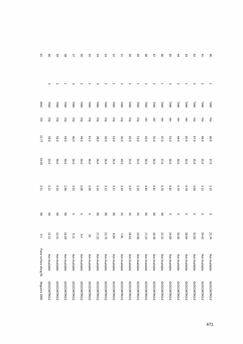
40 1
TAM
FAI 60.0
37.0 3.15
0 21.74
Not Available
GEOCO
NTRO
LE
41 2
TAM
FAI 68.0
35.0 3.15
0 29.42
Not Available
GEOCO
NTRO
LE
42 3
TAM
FAI 67.0
35.0 3.04
0 32.03
Not Available
GEOCO
NTRO
LE
43 1
TAM
HH 65.0
36.0 4.79
0 18.94
Not Available
GEOCO
NTRO
LE
44 2
TAM
HH 44.0
36.0 4.70
0 26.93
Not Available
GEOCO
NTRO
LE
45 3
TAM
HH 53.0
36.0 4.82
0 24.69
Not Available
GEOCO
NTRO
LE
46 1
TAM
HH 47.0
37.0 4.76
90 22.15
Not Available
GEOCO
NTRO
LE
47 2
TAM
HH 55.0
36.0 4.81
90 18.39
Not Available
GEOCO
NTRO
LE
48 3
TAM
HH 43.0
36.0 4.83
90 17.23
Not Available
GEOCO
NTRO
LE
49 1
TAM
FQI
53.0 35.0
3.16 45
14.96 N
ot Available GEO
CON
TROLE
50 2
TAM
FQI
43.0 35.0
3.07 45
16.62 N
ot Available GEO
CON
TROLE
51 3
TAM
FQI
35.0 34.0
3.29 45
7.81 N
ot Available GEO
CON
TROLE
52 1
TAM
FQI
53.0 36.0
3.21 90
8.94 N
ot Available GEO
CON
TROLE
53 2
TAM
FQI
50.0 36.0
3.12 90
15.74 N
ot Available GEO
CON
TROLE
54 3
TAM
FQI
38.0 36.0
3.16 90
17.23 N
ot Available GEO
CON
TROLE
55 1
TAM
FQI
61.0 36.0
3.00 0
20 N
ot Available GEO
CON
TROLE
56 2
TAM
FQI
44.0 36.0
3.00 0
9.4 N
ot Available GEO
CON
TROLE
57 3
TAM
FQI
40.0 36.0
3.03 0
9.15 N
ot Available GEO
CON
TROLE
58 1
TAM
FQI
59.0 36.0
2.96 90
16.69 N
ot Available GEO
CON
TROLE
59 2
TAM
FQI
56.0 36.0
3.10 90
12.41 N
ot Available GEO
CON
TROLE
60 3
TAM
FQI
39.0 35.0
3.21 90
12.51 N
ot Available GEO
CON
TROLE
61 M
AC FDI
22.77 54.05
3.31 90
9.5 Plane surface along Sb
Nogueira 2000
471
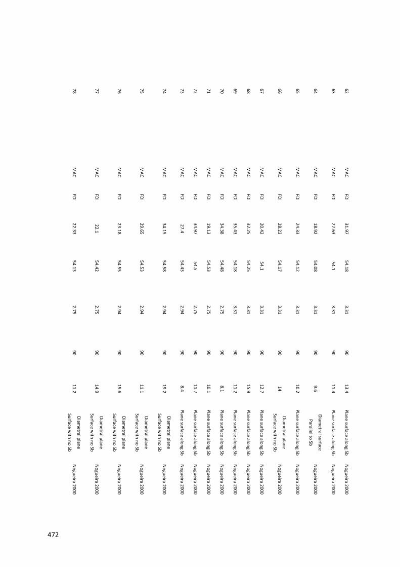
62 M
AC FDI
31.97 54.18
3.31 90
13.4 Plane surface along Sb
Nogueira 2000
63 M
AC FDI
27.63 54.1
3.31 90
11.4 Plane surface along Sb
Nogueira 2000
64 M
AC FDI
18.92 54.08
3.31 90
9.6 Diam
etral surface
Parallel to Sb N
ogueira 2000
65 M
AC FDI
24.33 54.12
3.31 90
10.2 Plane surface along Sb
Nogueira 2000
66 M
AC FDI
28.23 54.17
3.31 90
14 Diam
etral plane
Surface with no Sb
Nogueira 2000
67 M
AC FDI
20.42 54.1
3.31 90
12.7 Plane surface along Sb
Nogueira 2000
68 M
AC FDI
32.25 54.25
3.31 90
15.9 Plane surface along Sb
Nogueira 2000
69 M
AC FDI
35.43 54.18
3.31 90
11.2 Plane surface along Sb
Nogueira 2000
70 M
AC FDI
34.38 54.48
2.75 90
8.1 Plane surface along Sb
Nogueira 2000
71 M
AC FDI
19.13 54.53
2.75 90
10.1 Plane surface along Sb
Nogueira 2000
72 M
AC FDI
34.97 54.5
2.75 90
11.7 Plane surface along Sb
Nogueira 2000
73 M
AC FDI
27.4 54.43
2.94 90
8.4 Plane surface along Sb
Nogueira 2000
74 M
AC FDI
34.15 54.58
2.94 90
19.2 Diam
etral plane
Surface with no Sb
Nogueira 2000
75 M
AC FDI
29.65 54.53
2.94 90
11.1 Diam
etral plane
Surface with no Sb
Nogueira 2000
76 M
AC FDI
23.18 54.55
2.94 90
15.6 Diam
etral plane
Surface with no Sb
Nogueira 2000
77 M
AC FDI
22.1 54.42
2.75 90
14.9 Diam
etral plane
Surface with no Sb
Nogueira 2000
78 M
AC FDI
22.33 54.13
2.75 90
11.2 Diam
etral plane
Surface with no Sb
Nogueira 2000
472
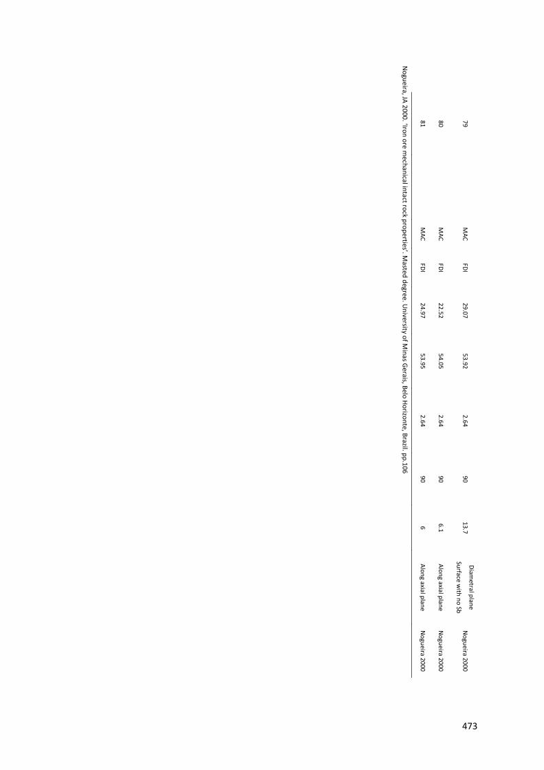
79 M
AC FDI
29.07 53.92
2.64 90
13.7 Diam
etral plane
Surface with no Sb
Nogueira 2000
80 M
AC FDI
22.52 54.05
2.64 90
6.1 Along axial plane
Nogueira 2000
81 M
AC FDI
24.97 53.95
2.64 90
6 Along axial plane
Nogueira 2000
Nogueira, JA 2000. ‘Iron ore m
echanical intact rock properties’. Masted degree. U
niversity of Minas Gerais, Belo Horizonte, Brazil. pp.106
473

474
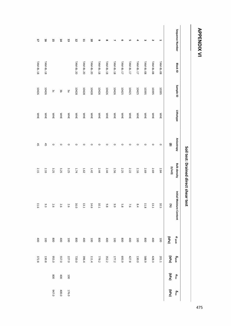
APPENDIX VI
Soil test: Drained direct shear test
Sequence Num
ber Block ID
Sam
ple ID Lithotype
Anisotropy
(β)
Bulk density
(t/m3)
Initial Moisture Content
(%)
σ peak
(kPa)
δpeak
(kPa)
σres
(kPa)
δres
(kPa)
1 TAM
-BL-08 10395
WHE
0 2.84
10.5 100
201.1
2 TAM
-BL-08 10395
WHE
0 2.69
13.1 400
428.3
3 TAM
-BL-08 10395
WHE
0 2.69
11.8 800
588.9
4 TAM
-BL-17 10425
WHE
0 2.16
8.4 100
130.0
5 TAM
-BL-17 10425
WHE
0 2.22
7.6 400
427.8
6 TAM
-BL-17 10425
WHE
0 2.25
5.8 800
693.9
7 TAM
-BL-18 10426
WHE
0 2.56
9.9 100
177.2
8 TAM
-BL-18 10426
WHE
0 2.44
9.8 400
352.2
9 TAM
-BL-18 10426
WHE
0 2.44
10.1 800
779.2
10 TAM
-BL-20 10428
WHE
0 1.42
14.6 100
111.4
11 TAM
-BL-20 10428
WHE
0 1.62
13.1 400
396.4
12 TAM
-BL-20 10428
WHE
0 1.74
16.0 800
720.0
13 3a
WHE
0 3.25
2.6 100
227.0 100
176.0
14 3b
WHE
0 3.25
2.6 400
557.0 400
400.0
15 3c
WHE
0 3.25
2.6 800
955.0 800
947.0
16 TAM
-BL-18 10426
WHE
45 2.33
9.3 100
130.8
17 TAM
-BL-18 10426
WHE
45 2.15
11.6 400
372.8
475
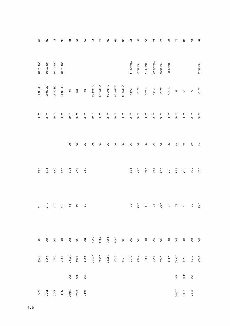
18 TAM
-BL-18 10426
WHE
45 2.25
10.8 800
631.4
19 5a
WHE
45 3.32
3.7 100
323.0 100
292.0
20 5b
WHE
45 3.32
3.7 400
658.0 400
571.0
21 5c
WHE
45 3.32
3.7 800
1243.0 800
1145.0
22 TAM
-BL-08 10395
WHE
90 3.12
9.0 100
208.6
23 TAM
-BL-08 10395
WHE
90 2.74
13.7 400
379.2
24 TAM
-BL-08 10395
WHE
90 2.82
9.5 800
803.3
25 TAM
-BL-17 10425
WHE
90 2.66
9.4 100
136.3
26 TAM
-BL-17 10425
WHE
90 2.67
10.3 400
445.6
27 TAM
-BL-17 10425
WHE
90 2.26
8.0 800
616.7
28 2.1194.04
WHE
90 502
528.0
29 2.1197.04
WHE
90 1002
930.0
30 2.1200.04
WHE
90 2002
1779.0
31 2.1199.04
WHE
90 4013
2759.0
32 2.1198.04
WHE
90 7025
4420.0
33 10a
WHE
90 3.27
3.6 100
243.0 100
164.0
34 10b
WHE
90 3.27
3.6 400
626.0 400
510.0
35 10c
WHE
90 3.27
3.6 800
1229.0 800
1210.0
36 JAN
PC -03 CIS 08-17
WHE
2.20 11.9
100 138.5
99.8
37 JAN
PC -03 CIS 08-17
WHE
2.47 11.9
200 221.2
220.0
38 JAN
PC -03 CIS 08-17
WHE
2.19 11.9
400 435.0
428.0
39 JAN
PC -03 CIS 08-17
WHE
2.60 11.9
800 628.0
622.0
476
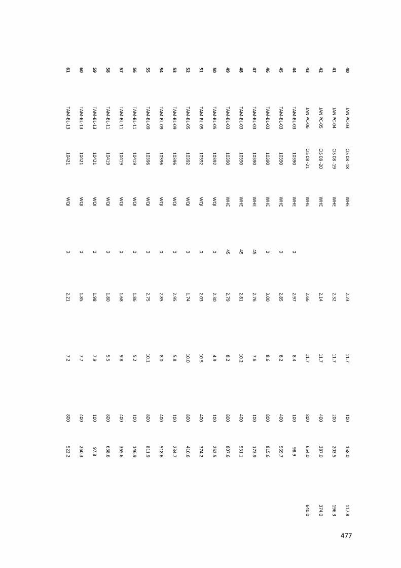
40 JAN
PC-03 CIS 08 -18
WHE
2.23 11.7
100 158.0
117.8
41 JAN
PC-04 CIS 08 -19
WHE
2.32 11.7
200 203.5
196.3
42 JAN
PC-05 CIS 08 -20
WHE
2.14 11.7
400 387.0
374.0
43 JAN
PC-06 CIS 08 -21
WHE
2.66 11.7
800 654.0
640.0
44 TAM
-BL-03 10390
WHE
0 2.97
8.4 100
98.9
45 TAM
-BL-03 10390
WHE
0 2.85
8.2 400
569.7
46 TAM
-BL-03 10390
WHE
0 3.00
8.6 800
815.6
47 TAM
-BL-03 10390
WHE
45 2.76
7.6 100
173.9
48 TAM
-BL-03 10390
WHE
45 2.81
10.2 400
531.1
49 TAM
-BL-03 10390
WHE
45 2.79
8.2 800
807.6
50 TAM
-BL-05 10392
WQ
I 0
2.30 4.9
100 252.5
51 TAM
-BL-05 10392
WQ
I 0
2.03 10.5
400 374.2
52 TAM
-BL-05 10392
WQ
I 0
1.74 10.0
800 410.6
53 TAM
-BL-09 10396
WQ
I 0
2.95 5.8
100 234.7
54 TAM
-BL-09 10396
WQ
I 0
2.85 8.0
400 518.6
55 TAM
-BL-09 10396
WQ
I 0
2.75 10.1
800 811.9
56 TAM
-BL-11 10419
WQ
I 0
1.86 5.2
100 146.9
57 TAM
-BL-11 10419
WQ
I 0
1.68 9.8
400 365.6
58 TAM
-BL-11 10419
WQ
I 0
1.80 5.5
800 638.6
59 TAM
-BL-13 10421
WQ
I 0
1.98 7.9
100 97.8
60 TAM
-BL-13 10421
WQ
I 0
1.85 7.7
400 260.3
61 TAM
-BL-13 10421
WQ
I 0
2.21 7.2
800 522.2
477
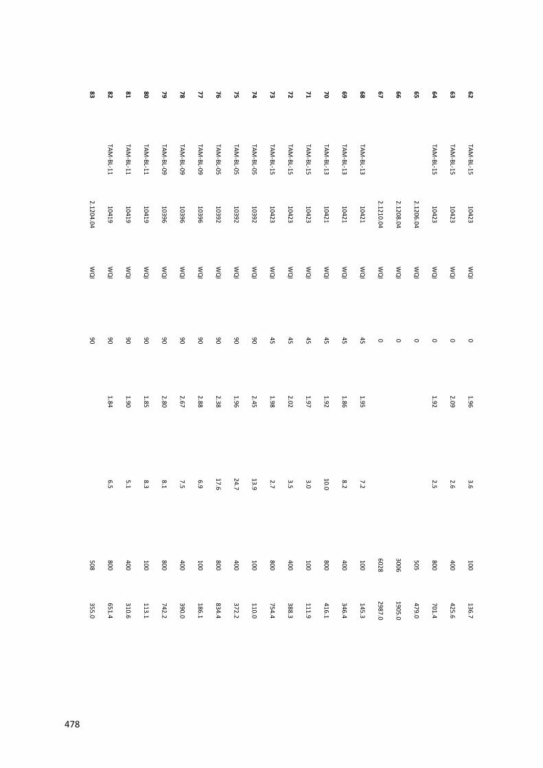
62 TAM
-BL-15 10423
WQ
I 0
1.96 3.6
100 136.7
63 TAM
-BL-15 10423
WQ
I 0
2.09 2.6
400 425.6
64 TAM
-BL-15 10423
WQ
I 0
1.92 2.5
800 701.4
65 2.1206.04
WQ
I 0
505 479.0
66 2.1208.04
WQ
I 0
3006 1905.0
67 2.1210.04
WQ
I 0
6028 2987.0
68 TAM
-BL-13 10421
WQ
I 45
1.95 7.2
100 145.3
69 TAM
-BL-13 10421
WQ
I 45
1.86 8.2
400 346.4
70 TAM
-BL-13 10421
WQ
I 45
1.92 10.0
800 416.1
71 TAM
-BL-15 10423
WQ
I 45
1.97 3.0
100 111.9
72 TAM
-BL-15 10423
WQ
I 45
2.02 3.5
400 388.3
73 TAM
-BL-15 10423
WQ
I 45
1.98 2.7
800 754.4
74 TAM
-BL-05 10392
WQ
I 90
2.45 13.9
100 110.0
75 TAM
-BL-05 10392
WQ
I 90
1.96 24.7
400 372.2
76 TAM
-BL-05 10392
WQ
I 90
2.38 17.6
800 834.4
77 TAM
-BL-09 10396
WQ
I 90
2.88 6.9
100 186.1
78 TAM
-BL-09 10396
WQ
I 90
2.67 7.5
400 390.0
79 TAM
-BL-09 10396
WQ
I 90
2.80 8.1
800 742.2
80 TAM
-BL-11 10419
WQ
I 90
1.85 8.3
100 113.1
81 TAM
-BL-11 10419
WQ
I 90
1.90 5.1
400 310.6
82 TAM
-BL-11 10419
WQ
I 90
1.84 6.5
800 651.4
83 2.1204.04
WQ
I 90
508 355.0
478
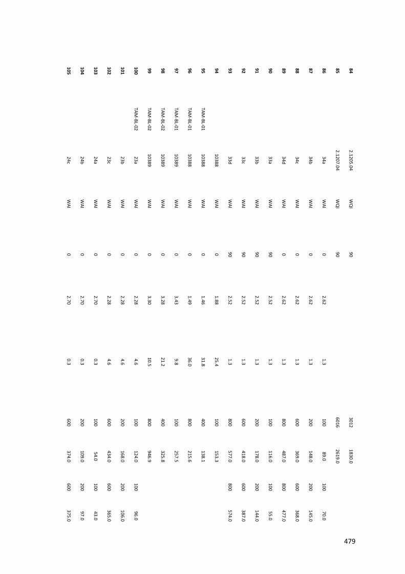
84 2.1205.04
WQ
I 90
3012 1830.0
85 2.1207.04
WQ
I 90
6016 2619.0
86 34a
WAI
0 2.62
1.3 100
89.0 100
70.0
87 34b
WAI
0 2.62
1.3 200
148.0 200
145.0
88 34c
WAI
0 2.62
1.3 600
369.0 600
368.0
89 34d
WAI
0 2.62
1.3 800
487.0 800
477.0
90 33a
WAI
90 2.52
1.3 100
116.0 100
55.0
91 33b
WAI
90 2.52
1.3 200
178.0 200
144.0
92 33c
WAI
90 2.52
1.3 600
418.0 600
387.0
93 33d
WAI
90 2.52
1.3 800
577.0 800
574.0
94 10388
WAI
0 1.88
25.4 100
153.3
95 TAM
-BL-01 10388
WAI
0 1.46
31.8 400
138.1
96 TAM
-BL-01 10388
WAI
0 1.49
36.0 800
215.6
97 TAM
-BL-01 10389
WAI
0 3.43
9.8 100
257.5
98 TAM
-BL-02 10389
WAI
0 3.28
21.2 400
325.8
99 TAM
-BL-02 10389
WAI
0 3.30
10.5 800
946.9
100 TAM
-BL-02 23a
WAI
0 2.28
4.6 100
124.0 100
96.0
101 23b
WAI
0 2.28
4.6 200
168.0 200
106.0
102 23c
WAI
0 2.28
4.6 600
434.0 600
365.0
103 24a
WAI
0 2.70
0.3 100
54.0 100
43.0
104 24b
WAI
0 2.70
0.3 200
109.0 200
97.0
105 24c
WAI
0 2.70
0.3 600
374.0 600
375.0
479
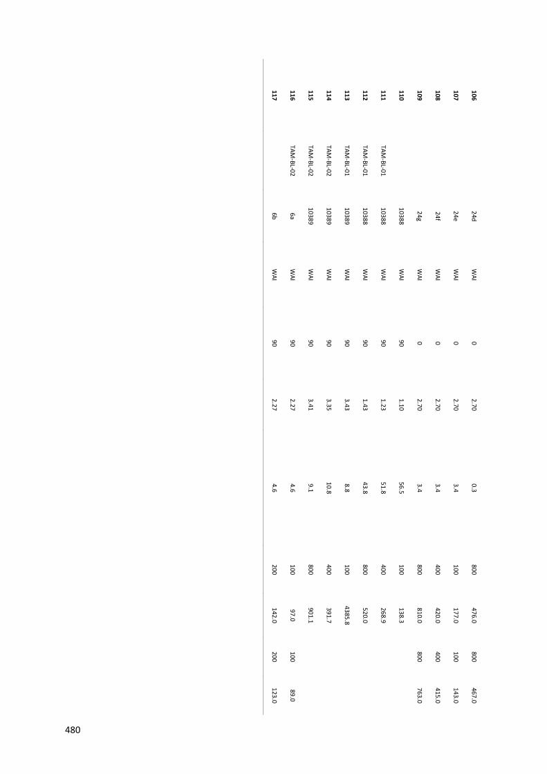
106 24d
WAI
0 2.70
0.3 800
476.0 800
467.0
107 24e
WAI
0 2.70
3.4 100
177.0 100
143.0
108 24f
WAI
0 2.70
3.4 400
420.0 400
415.0
109 24g
WAI
0 2.70
3.4 800
810.0 800
763.0
110 10388
WAI
90 1.10
56.5 100
138.3
111 TAM
-BL-01 10388
WAI
90 1.23
51.8 400
268.9
112 TAM
-BL-01 10388
WAI
90 1.43
43.8 800
520.0
113 TAM
-BL-01 10389
WAI
90 3.43
8.8 100
4385.8
114 TAM
-BL-02 10389
WAI
90 3.35
10.8 400
391.7
115 TAM
-BL-02 10389
WAI
90 3.41
9.1 800
901.1
116 TAM
-BL-02 6a
WAI
90 2.27
4.6 100
97.0 100
89.0
117 6b
WAI
90 2.27
4.6 200
142.0 200
123.0
480
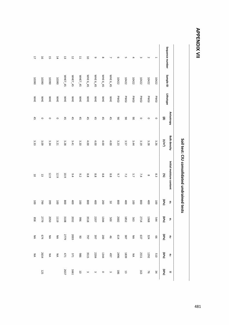
APPENDIX VII
Soil test: CIU consolidated undrained tests
Sequence number
Sample ID
Lithotype Anisotropy
(β)
Bulk density
(t/m3)
Initial moisture content
(%)
σ3
(kPa)
σ1
(kPa)
σ3'
(kPa)
σ1'
(kPa)
U
(kPa)
1 10422
PWGI
0 3.26
8.3 100
544 66
510 34
2 10422
PWGI
0 3.28
8 400
1368 324
1292 76
3 10422
PWGI
0 3.19
7.4 800
2714 637
2551 163
4 10422
PWGI
90 3.44
5.7 100
563 N
A N
A
5 10422
PWGI
90 3.57
7.2 400
1852 387
1839 13
6 10422
PWGI
90 3.23
9.7 800
2682 614
2496 186
7 W
HE 6_45 W
HE 45
4.00 8.8
50 500
46 497
3
8 W
HE 6_45 W
HE 45
4.00 8.8
200 1344
200 1344
0
9 W
HE 6_45 W
HE 45
4.00 8.8
400 2207
397 2204
3
10 W
HE 6_45 W
HE 45
4.00 8.8
800 3518
797 3515
3
11 W
HE7_45 W
HE 45
3.20 9.2
100 996
90 986
10
12 W
HE7_45 W
HE 45
3.41 9.4
400 2032
2003 371
1661
13 W
HE7_45 W
HE 45
3.28 10.9
800 3108
2779 471
2637
14 10390
WHE
0 3.21
12.9 100
1119 N
A N
A
15 10390
WHE
0 3.34
12.9 399
2050 N
A N
A
16 10390
WHE
0 3.09
13 799
2779 674
2654 125
17 10390
WHE
45 3.33
10 100
858 N
A N
A
481
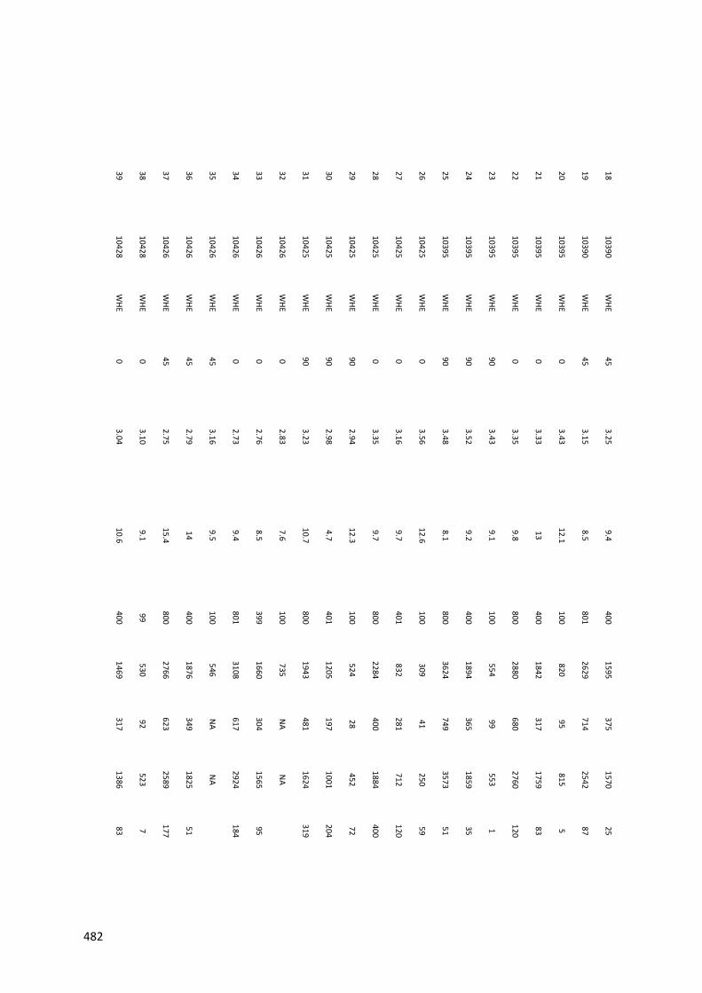
18 10390
WHE
45 3.25
9.4 400
1595 375
1570 25
19 10390
WHE
45 3.15
8.5 801
2629 714
2542 87
20 10395
WHE
0 3.43
12.1 100
820 95
815 5
21 10395
WHE
0 3.33
13 400
1842 317
1759 83
22 10395
WHE
0 3.35
9.8 800
2880 680
2760 120
23 10395
WHE
90 3.43
9.1 100
554 99
553 1
24 10395
WHE
90 3.52
9.2 400
1894 365
1859 35
25 10395
WHE
90 3.48
8.1 800
3624 749
3573 51
26 10425
WHE
0 3.56
12.6 100
309 41
250 59
27 10425
WHE
0 3.16
9.7 401
832 281
712 120
28 10425
WHE
0 3.35
9.7 800
2284 400
1884 400
29 10425
WHE
90 2.94
12.3 100
524 28
452 72
30 10425
WHE
90 2.98
4.7 401
1205 197
1001 204
31 10425
WHE
90 3.23
10.7 800
1943 481
1624 319
32 10426
WHE
0 2.83
7.6 100
735 N
A N
A
33 10426
WHE
0 2.76
8.5 399
1660 304
1565 95
34 10426
WHE
0 2.73
9.4 801
3108 617
2924 184
35 10426
WHE
45 3.16
9.5 100
546 N
A N
A
36 10426
WHE
45 2.79
14 400
1876 349
1825 51
37 10426
WHE
45 2.75
15.4 800
2766 623
2589 177
38 10428
WHE
0 3.10
9.1 99
530 92
523 7
39 10428
WHE
0 3.04
10.6 400
1469 317
1386 83
482
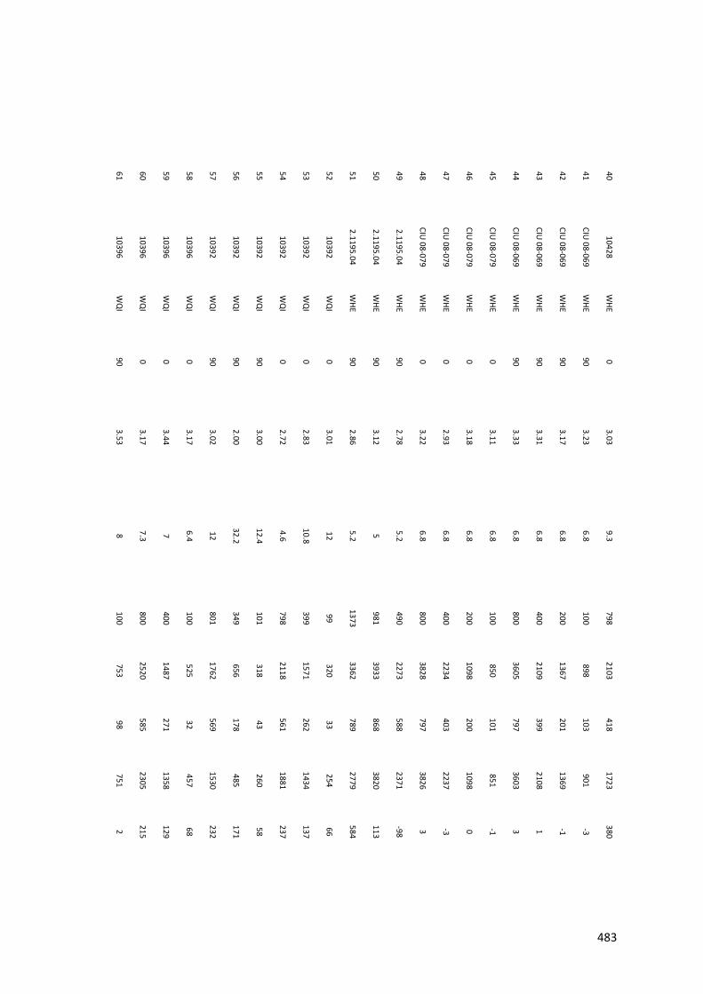
40 10428
WHE
0 3.03
9.3 798
2103 418
1723 380
41 CIU
08-069 W
HE 90
3.23 6.8
100 898
103 901
-3
42 CIU
08-069 W
HE 90
3.17 6.8
200 1367
201 1369
-1
43 CIU
08-069 W
HE 90
3.31 6.8
400 2109
399 2108
1
44 CIU
08-069 W
HE 90
3.33 6.8
800 3605
797 3603
3
45 CIU
08-079 W
HE 0
3.11 6.8
100 850
101 851
-1
46 CIU
08-079 W
HE 0
3.18 6.8
200 1098
200 1098
0
47 CIU
08-079 W
HE 0
2.93 6.8
400 2234
403 2237
-3
48 CIU
08-079 W
HE 0
3.22 6.8
800 3828
797 3826
3
49 2.1195.04
WHE
90 2.78
5.2 490
2273 588
2371 -98
50 2.1195.04
WHE
90 3.12
5 981
3933 868
3820 113
51 2.1195.04
WHE
90 2.86
5.2 1373
3362 789
2779 584
52 10392
WQ
I 0
3.01 12
99 320
33 254
66
53 10392
WQ
I 0
2.83 10.8
399 1571
262 1434
137
54 10392
WQ
I 0
2.72 4.6
798 2118
561 1881
237
55 10392
WQ
I 90
3.00 12.4
101 318
43 260
58
56 10392
WQ
I 90
2.00 32.2
349 656
178 485
171
57 10392
WQ
I 90
3.02 12
801 1762
569 1530
232
58 10396
WQ
I 0
3.17 6.4
100 525
32 457
68
59 10396
WQ
I 0
3.44 7
400 1487
271 1358
129
60 10396
WQ
I 0
3.17 7.3
800 2520
585 2305
215
61 10396
WQ
I 90
3.53 8
100 753
98 751
2
483
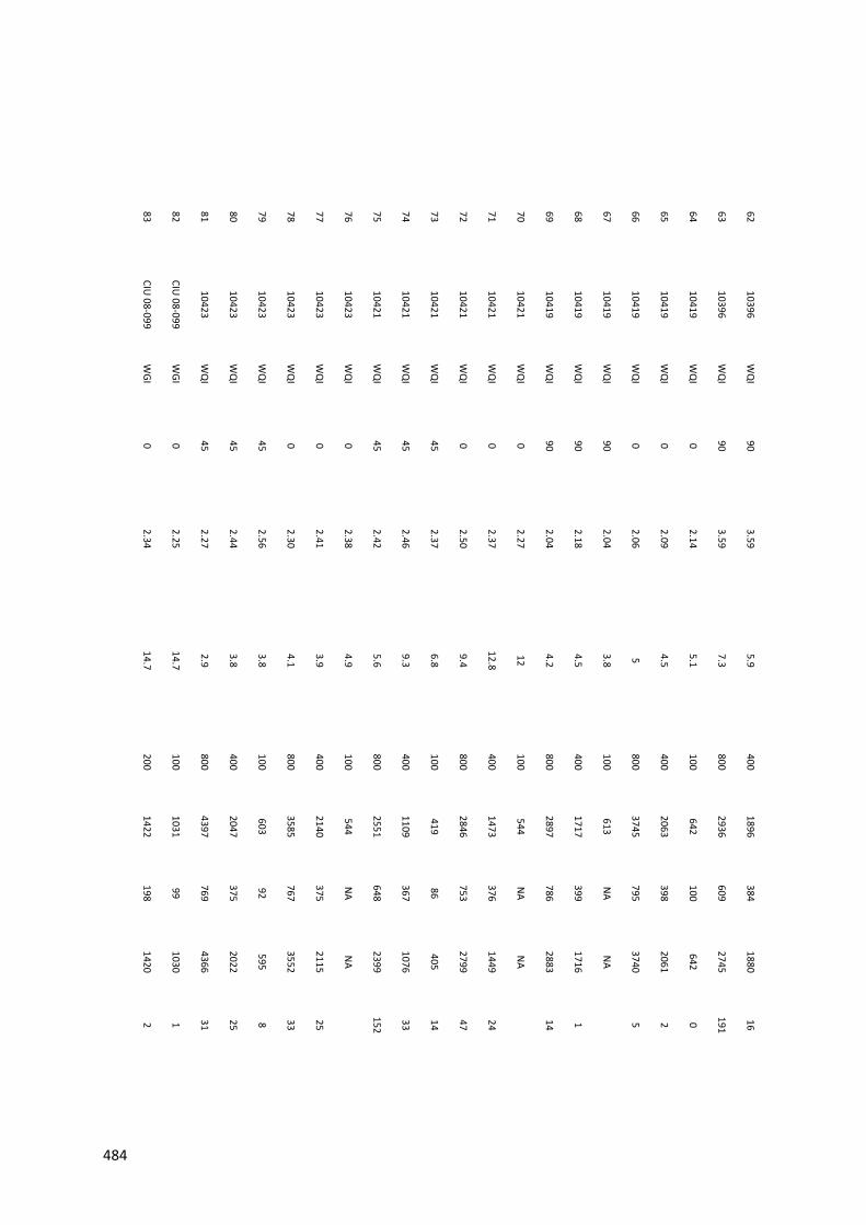
62 10396
WQ
I 90
3.59 5.9
400 1896
384 1880
16
63 10396
WQ
I 90
3.59 7.3
800 2936
609 2745
191
64 10419
WQ
I 0
2.14 5.1
100 642
100 642
0
65 10419
WQ
I 0
2.09 4.5
400 2063
398 2061
2
66 10419
WQ
I 0
2.06 5
800 3745
795 3740
5
67 10419
WQ
I 90
2.04 3.8
100 613
NA
NA
68 10419
WQ
I 90
2.18 4.5
400 1717
399 1716
1
69 10419
WQ
I 90
2.04 4.2
800 2897
786 2883
14
70 10421
WQ
I 0
2.27 12
100 544
NA
NA
71 10421
WQ
I 0
2.37 12.8
400 1473
376 1449
24
72 10421
WQ
I 0
2.50 9.4
800 2846
753 2799
47
73 10421
WQ
I 45
2.37 6.8
100 419
86 405
14
74 10421
WQ
I 45
2.46 9.3
400 1109
367 1076
33
75 10421
WQ
I 45
2.42 5.6
800 2551
648 2399
152
76 10423
WQ
I 0
2.38 4.9
100 544
NA
NA
77 10423
WQ
I 0
2.41 3.9
400 2140
375 2115
25
78 10423
WQ
I 0
2.30 4.1
800 3585
767 3552
33
79 10423
WQ
I 45
2.56 3.8
100 603
92 595
8
80 10423
WQ
I 45
2.44 3.8
400 2047
375 2022
25
81 10423
WQ
I 45
2.27 2.9
800 4397
769 4366
31
82 CIU
08-099 W
GI 0
2.25 14.7
100 1031
99 1030
1
83 CIU
08-099 W
GI 0
2.34 14.7
200 1422
198 1420
2
484
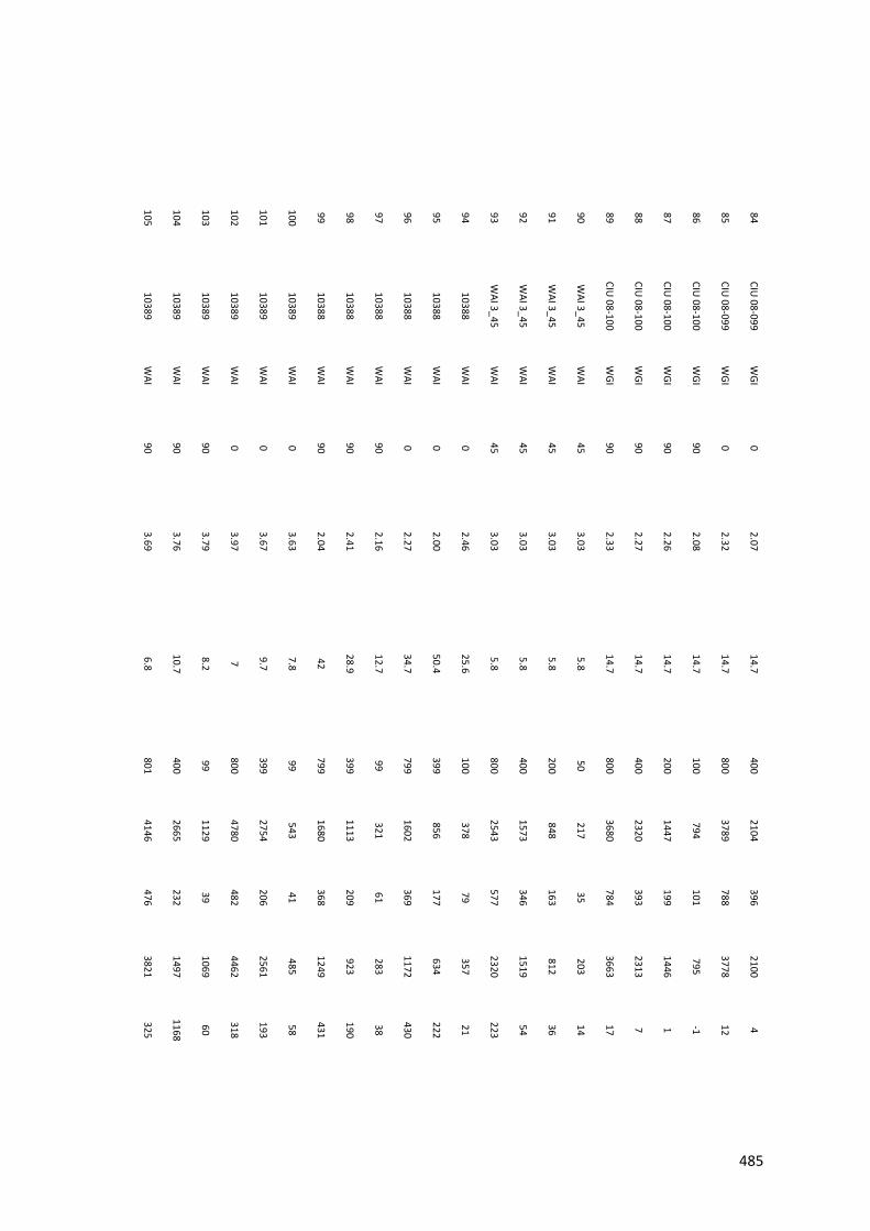
84 CIU
08-099 W
GI 0
2.07 14.7
400 2104
396 2100
4
85 CIU
08-099 W
GI 0
2.32 14.7
800 3789
788 3778
12
86 CIU
08-100 W
GI 90
2.08 14.7
100 794
101 795
-1
87 CIU
08-100 W
GI 90
2.26 14.7
200 1447
199 1446
1
88 CIU
08-100 W
GI 90
2.27 14.7
400 2320
393 2313
7
89 CIU
08-100 W
GI 90
2.33 14.7
800 3680
784 3663
17
90 W
AI 3_45 W
AI 45
3.03 5.8
50 217
35 203
14
91 W
AI 3_45 W
AI 45
3.03 5.8
200 848
163 812
36
92 W
AI 3_45 W
AI 45
3.03 5.8
400 1573
346 1519
54
93 W
AI 3_45 W
AI 45
3.03 5.8
800 2543
577 2320
223
94 10388
WAI
0 2.46
25.6 100
378 79
357 21
95 10388
WAI
0 2.00
50.4 399
856 177
634 222
96 10388
WAI
0 2.27
34.7 799
1602 369
1172 430
97 10388
WAI
90 2.16
12.7 99
321 61
283 38
98 10388
WAI
90 2.41
28.9 399
1113 209
923 190
99 10388
WAI
90 2.04
42 799
1680 368
1249 431
100 10389
WAI
0 3.63
7.8 99
543 41
485 58
101 10389
WAI
0 3.67
9.7 399
2754 206
2561 193
102 10389
WAI
0 3.97
7 800
4780 482
4462 318
103 10389
WAI
90 3.79
8.2 99
1129 39
1069 60
104 10389
WAI
90 3.76
10.7 400
2665 232
1497 1168
105 10389
WAI
90 3.69
6.8 801
4146 476
3821 325
485
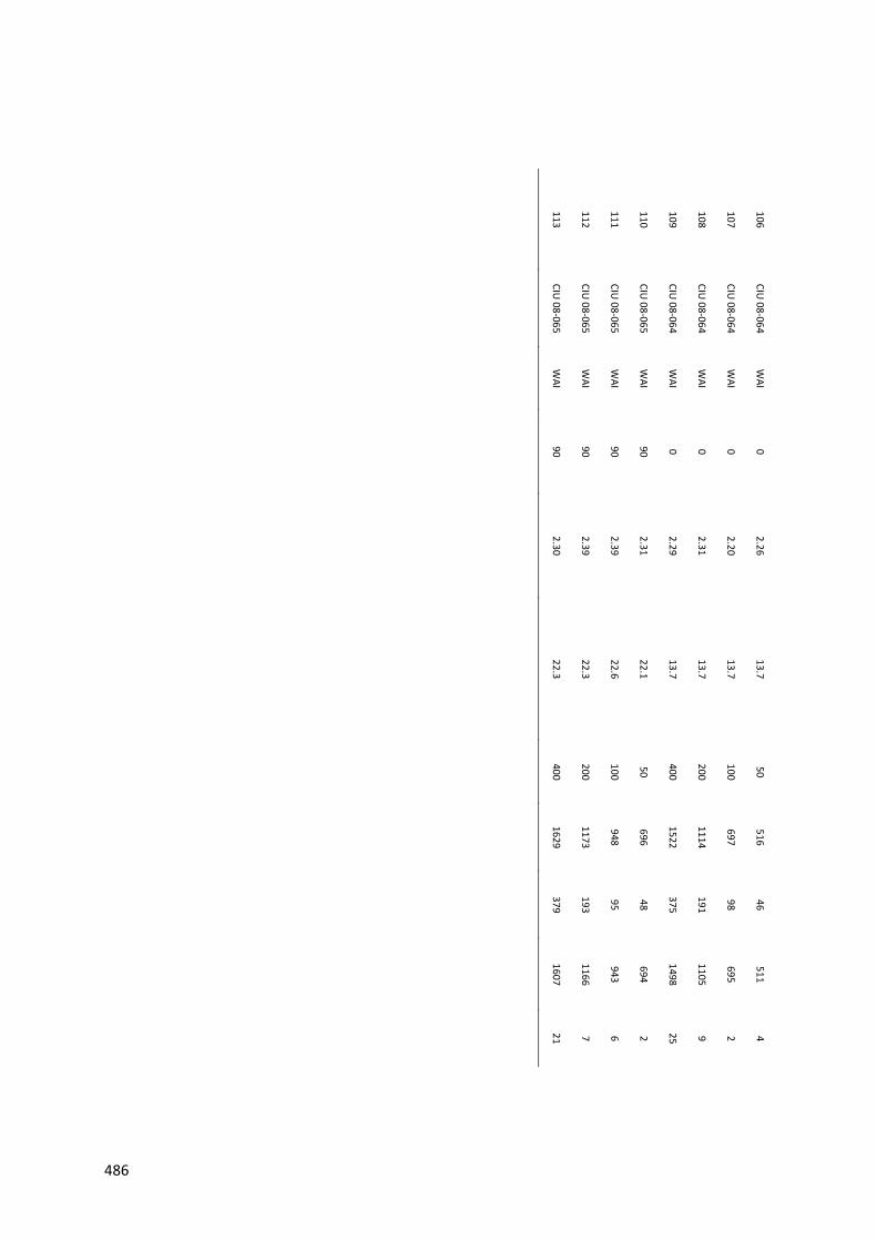
106 CIU
08-064 W
AI 0
2.26 13.7
50 516
46 511
4
107 CIU
08-064 W
AI 0
2.20 13.7
100 697
98 695
2
108 CIU
08-064 W
AI 0
2.31 13.7
200 1114
191 1105
9
109 CIU
08-064 W
AI 0
2.29 13.7
400 1522
375 1498
25
110 CIU
08-065 W
AI 90
2.31 22.1
50 696
48 694
2
111 CIU
08-065 W
AI 90
2.39 22.6
100 948
95 943
6
112 CIU
08-065 W
AI 90
2.39 22.3
200 1173
193 1166
7
113 CIU
08-065 W
AI 90
2.30 22.3
400 1629
379 1607
21
486
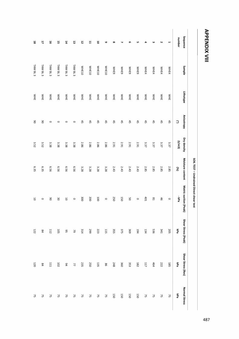
APPENDIX VIII
SOIL TEST – U
ndrained Direct shear test
Sequence
number
Sample
Lithotype Anisotropy
(°)
Dry density
(t/m3)
Moisture content
(%)
Matric suction (Peak)
- kPa
Shear Stress (Peak)
kPa
Shear Stress (Res)
kPa
Norm
al Stress
kPa
1 W
HE4 W
HE 45
3.37 2.85
0 205
185 75
2 W
HE4 W
HE 45
3.37 2.85
46 341
222 75
3 W
HE4 W
HE 45
3.37 2.85
81 536
464 75
4 W
HE4 W
HE 45
3.37 2.85
401 134
117 75
5 W
HE9 W
HE 45
2.91 2.43
0 194
182 150
6 W
HE9 W
HE 45
2.91 2.43
50 369
353 150
7 W
HE9 W
HE 45
2.91 2.43
150 375
360 150
8 W
HE9 W
HE 45
2.91 2.43
250 355
248 150
9 W
HE10 W
HE 45
2.86 3.28
0 115
86 75
10 W
HE10 W
HE 45
2.86 3.28
100 223
135 75
11 W
HE10 W
HE 45
2.86 3.28
200 299
250 75
12 W
HE10 W
HE 45
2.86 3.28
300 314
235 75
13 TAM
BL 3 W
HE 0
3.38 6.56
0 79
77 75
14 TAM
BL 3 W
HE 0
3.38 6.56
10 95
94 75
15 TAM
BL 3 W
HE 0
3.38 6.56
30 105
102 75
16 TAM
BL 3 W
HE 0
3.38 6.56
90 112
111 75
17 TAM
BL 3 W
HE 90
3.52 6.35
0 84
84 75
18 TAM
BL 3 W
HE 90
3.52 6.35
10 122
120 75
487
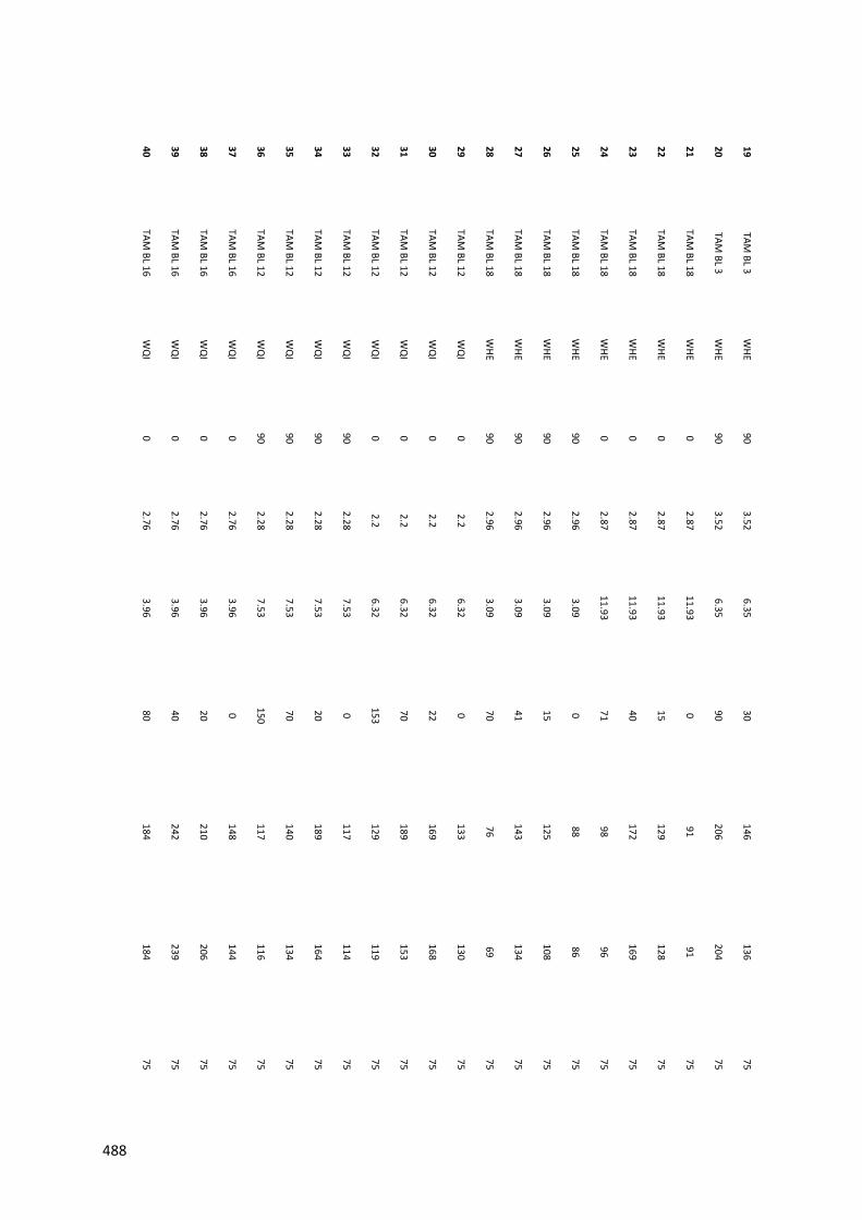
19 TAM
BL 3 W
HE 90
3.52 6.35
30 146
136 75
20 TAM
BL 3 W
HE 90
3.52 6.35
90 206
204 75
21 TAM
BL 18 W
HE 0
2.87 11.93
0 91
91 75
22 TAM
BL 18 W
HE 0
2.87 11.93
15 129
128 75
23 TAM
BL 18 W
HE 0
2.87 11.93
40 172
169 75
24 TAM
BL 18 W
HE 0
2.87 11.93
71 98
96 75
25 TAM
BL 18 W
HE 90
2.96 3.09
0 88
86 75
26 TAM
BL 18 W
HE 90
2.96 3.09
15 125
108 75
27 TAM
BL 18 W
HE 90
2.96 3.09
41 143
134 75
28 TAM
BL 18 W
HE 90
2.96 3.09
70 76
69 75
29 TAM
BL 12 W
QI
0 2.2
6.32 0
133 130
75
30 TAM
BL 12 W
QI
0 2.2
6.32 22
169 168
75
31 TAM
BL 12 W
QI
0 2.2
6.32 70
189 153
75
32 TAM
BL 12 W
QI
0 2.2
6.32 153
129 119
75
33 TAM
BL 12 W
QI
90 2.28
7.53 0
117 114
75
34 TAM
BL 12 W
QI
90 2.28
7.53 20
189 164
75
35 TAM
BL 12 W
QI
90 2.28
7.53 70
140 134
75
36 TAM
BL 12 W
QI
90 2.28
7.53 150
117 116
75
37 TAM
BL 16 W
QI
0 2.76
3.96 0
148 144
75
38 TAM
BL 16 W
QI
0 2.76
3.96 20
210 206
75
39 TAM
BL 16 W
QI
0 2.76
3.96 40
242 239
75
40 TAM
BL 16 W
QI
0 2.76
3.96 80
184 184
75
488
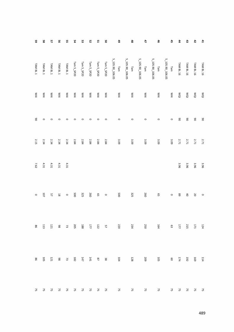
41 TAM
BL 16 W
QI
90 2.71
3.96 0
124 114
75
42 TAM
BL 16 W
QI
90 2.71
3.96 20
171 169
75
43 TAM
BL 16 W
QI
90 2.71
3.96 40
215 192
75
44 TAM
BL 16 W
QI
90 2.71
3.96 89
177 174
75
45 Tam
5_105.90_106.05
WAI
0 3.09
0 63
60 75
46 Tam
5_105.90_106.05
WAI
0 3.09
65 164
105 75
47 Tam
5_105.90_106.05
WAI
0 3.09
260 250
209 75
48 Tam
5_105.90_106.05
WAI
0 3.09
325 234
128 75
49 Tam
5_105.90_106.05
WAI
0 3.09
500 220
104 75
50 Tam
5_SP20 W
AI 0
2.84 0
57 38
75
51 Ta m
5_SP20 W
AI 0
2.84 65
122 87
75
52 Tam
5_SP20 W
AI 0
2.84 260
177 141
75
53 Tam
5_SP20 W
AI 0
2.84 325
188 147
75
54 Tam
5_SP20 W
AI 0
2.84 500
205 182
75
55 TAM
B L 1 W
AI 0
2.34 4.31
0 73
73 75
56 TAM
BL 1 W
AI 0
2.34 4.31
18 98
98 75
57 TAM
BL 1 W
AI 0
2.34 4.31
57 121
121 75
58 TAM
BL 1 W
AI 0
2.34 4.31
107 113
105 75
59 TAM
BL 1 W
AI 90
2.15 7.62
0 86
86 75
489
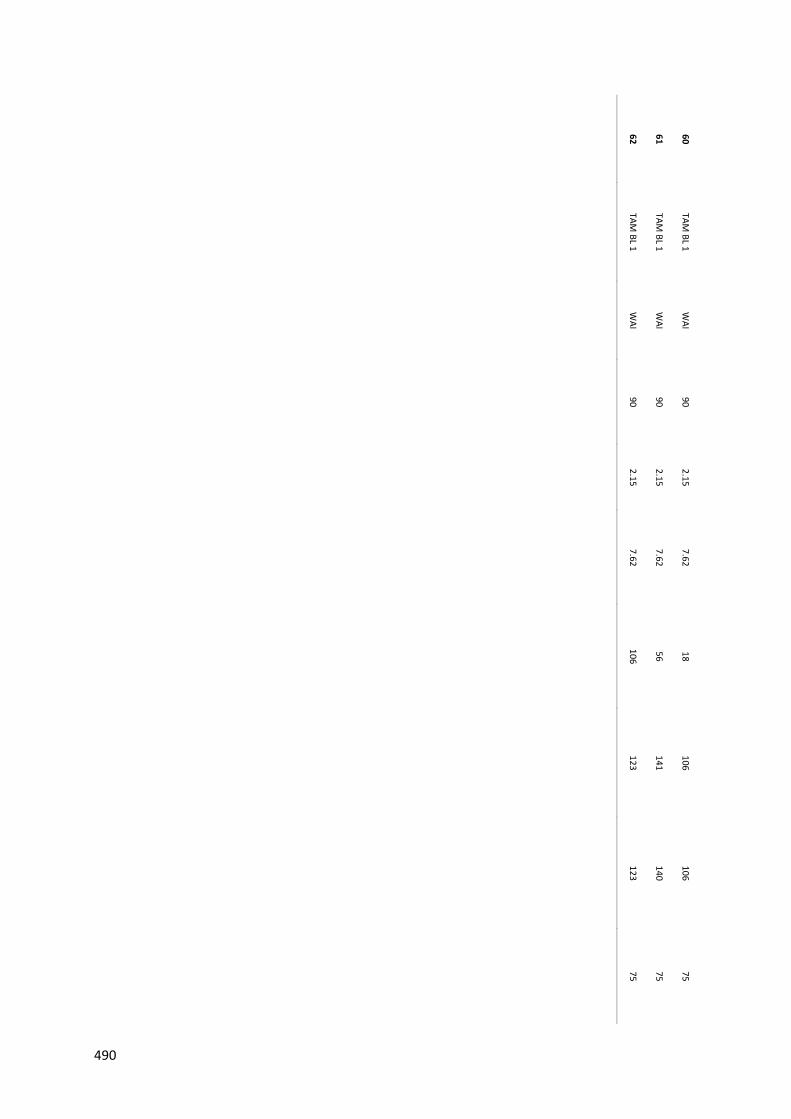
60 TAM
BL 1 W
AI 90
2.15 7.62
18 106
106 75
61 TAM
BL 1 W
AI 90
2.15 7.62
56 141
140 75
62 TAM
BL 1 W
AI 90
2.15 7.62
106 123
123 75
490


