Biotic vs. abiotic forcing on plankton assemblages varies with

available online at academic.oup.com/plankt

© The Author(s) 2020. Published by Oxford University Press. All rights reserved. For permissions, please e-mail: [email protected]

Journal of

Plankton Research academic.oup.com/plankt

J. Plankton Res. (2020) 42(2): 221–237. First published online March 5, 2020 doi:10.1093/plankt/fbaa010

ORIGINAL ARTICLE

Biotic vs. abiotic forcing on planktonassemblages varies with season and sizeclass in a large temperate estuary

GRETCHEN ROLLWAGEN-BOLLENS 1,2,*, STEPHEN BOLLENS1,2, ERIC DEXTER1,3 AND JEFFERY CORDELL4

1school of the environment, washington state university, vancouver, washington, 98686, usa 2school of biological sciences, washingtonstate university, vancouver, washington, 98686, usa 3department of environmental sciences, university of basel, basel, switzerland4school of aquatic and fishery sciences, university of washington, seattle, washington, 98195, usa

*corresponding author: [email protected]

Received November 6, 2019; editorial decision February 10, 2020; accepted February 10, 2020

Corresponding editor: Xabier Irigoien

Large river estuaries experience multiple anthropogenic stressors. Understanding plankton community dynamics inthese estuaries provides insights into the patterns of natural variability and effects of human activity. We undertook a2-year study in the Columbia River Estuary to assess the potential impacts of abiotic and biotic factors on planktoniccommunity structure over multiple time scales. We measured microplankton and zooplankton abundance, biomassand composition monthly, concurrent with measurements of chlorophyll a, nutrient concentrations, temperatureand salinity, from a dock in the lower estuary. We then statistically assessed the associations among the abundancesof planktonic groups and environmental and biological factors. During the late spring high flow period of bothyears, the lower estuary was dominated by freshwater and low salinity-adapted planktonic taxa, and zooplanktongrazers were more strongly associated with the autotroph-dominated microplankton assemblage than abiotic factors.During the early winter period of higher salinity and lower flow, nutrient (P ) availability exerted a strong influence onmicroplankton taxa, while only temperature and upwelling strength were associated with the zooplankton assemblage.Our results indicate that the relative influence of biotic (grazers) and abiotic (salinity, flow, nutrients and upwelling)factors varies seasonally and inter-annually, and among different size classes in the estuarine food web.

KEYWORDS: Columbia River Estuary; plankton community structure; biotic vs. abiotic forcing

Dow

nloaded from https://academ

ic.oup.com/plankt/article-abstract/42/2/221/5781151 by guest on 30 April 2020

http://orcid.org/0000-0002-5127-5720

JOURNAL OF PLANKTON RESEARCH VOLUME 42 NUMBER 2 PAGES 221–237 2020

INTRODUCTION

Large river estuaries are characterized by the dynamicinterplay of physical, chemical, geological and biologicalprocesses, often occurring within the context of increas-ing human impacts, such as eutrophication, habitat dis-turbance, modification of river flow through impound-ments and diversions, introduction of non-native taxaand climate change (Kennish, 2002; Martínez et al., 2007;Robins et al., 2016). Planktonic organisms are the domi-nant primary and secondary producers in pelagic estuar-ine ecosystems, with generation times of days to weeks,and often the ‘first responders’ to these highly variableconditions. Thus, the manner in which different compo-nents of estuarine plankton communities vary across timemay provide important insights into patterns of naturalvariability and the effects of human activity on the baseof these increasingly stressed food webs (Richardson andSchoeman, 2004; Richardson, 2008).

Changes in plankton community structure maydirectly impact the viability and productivity of manyother ecologically, socially and commercially importantestuarine populations, as plankton comprise the dominantprey resource for early life history stages of fish (bothresident and transient migrators) and certain benthicinvertebrates (e.g. bivalve mollusks) (Richardson, 2008;Bollens et al., 2010; Cloern et al., 2014). In addition,anthropogenic impacts on estuarine systems can bemanifested in changes in abundance and diversity ofplankton. For instance, eutrophication, climate warmingand human-mediated variations in flow regime have beenassociated with increased frequency and magnitude ofharmful algal blooms in river estuaries (Carstensen et al.,2007; Bricker et al., 2008; Roy et al., 2016). Similarly,large river estuaries with major international ports areparticularly at risk of introduction of invasive aquaticspecies through ballast water release (Bollens et al., 2002,2012; Dexter and Bollens, 2019). Indeed, the impacts ofhuman activity have their largest effects on the top andthe bottom of food webs, and are often cascaded upwardand downward through the plankton in pelagic systems(Wollrab et al., 2012).

Both biotic (e.g. predation, competition, etc.) and abi-otic (e.g. temperature, salinity, turbidity, mixing, etc.) fac-tors influence the structure and abundance of the manyassemblages within planktonic communities, especially inestuaries, regardless of whether they are the result ofnatural variability or anthropogenic drivers. However,the relative impacts of these concurrently acting factors,and how their influence may vary over time, is not wellstudied or understood. [Note: We are using an ecologicalnomenclature modified from Stroud et al. (2015) to definecommunity as ‘a group of interacting species populations

occurring together in space’ and assemblage as ‘a taxo-nomically related and comparably sized group of speciespopulations that occur together in space’].

For example, a range of published studies describehow environmental factors drive changes in abundance,composition and successional patterns in large estuaries,but these have typically focused on only one size class orfunctional group of plankton, such as the phytoplankton,e.g. Rhode River (Gallegos et al., 2010), Schelde Estu-ary (Muylaert et al., 2000), Coruna Estuary (Bode et al.,2017); the microzooplankton, e.g. Bay of Biscay (Dupuyet al., 2011) or the meso- and microzooplankton, e.g.St. Lawrence Estuary (Laprise and Dodson, 1994), SanFrancisco Estuary (SFE) (Bollens et al., 2011), Willapa Bay(Graham and Bollens, 2010). Only a very small numberof studies report temporal changes across multiple assem-blages from picoplankton up to microzooplankton, e.g. inthe Cochin estuary (Sooria et al., 2015) and Bahia Blancaestuary (Barría de Cao et al., 2011). In both of thesecases, the investigators associated environmental condi-tions with the abundances of individual assemblages, butdid not assess the biotic factors that might also have influ-enced the distribution and abundance of those assem-blages.

The Columbia River Estuary (CRE) is the downstreamterminus of the Columbia-Snake River system, whosewatershed spans parts of seven states in the US PacificNorthwest and two provinces in western Canada. TheCRE is increasingly impacted by human activity, withdramatic increases in population within the watershedover the past 30 years, and extensive impoundments thathave changed the flow regime and associated transportof nutrients and other dissolved components downstream(Wise et al., 2007). The CRE is also the gatewaythrough which several species of endangered Pacificsalmonids migrate between the ocean and upstreamspawning grounds throughout the Columbia River Basin,and where juvenile salmonids feed on planktonic andemergent prey at key stages in their life histories (Kirnet al., 1985; Goertler et al., 2016). Yet, over the pasthalf century, only a handful of published studies haveexamined the dynamics of the plankton community inthe CRE (Haertel and Osterberg, 1967; Haertel et al.,1969; Neitzel et al., 1982; Jones et al., 1990; Simenstadet al., 1990a; Bollens et al., 2012; Breckenridge et al., 2015;Dexter et al., 2015). Despite its ecological and economicimportance to the region, the CRE has been relativelypoorly studied compared to other large river estuaries,particularly with regard to dynamic environmentalinfluences on the biological communities residing inand/or transiting through its waters.

To explore the interactions and relative influenceof biotic and abiotic factors on the estuarine plankton

222

Dow



G. ROLLWAGEN-BOLLENS ET AL. SYNAPTIC RECRUITMENT ENHANCES GAP TERMINATION RESPONSES IN AUDITORY CORTEX

community over a range of temporal scales, and specif-ically to address the current knowledge gap regardingsuch processes in the CRE, we sampled the planktonacross a wide size (∼2 μm to 2 mm) and functional(primary producers, primary and secondary consumers)range, and measured a variety of environmental factors,at a single location in the lower CRE on a monthlybasis over a 2-year period (2005–2006). Using thesedata, our goal was to address three inter-related researchquestions:

1. What are the biotic (primary producers, consumers)and abiotic (river flow, salinity, temperature, etc.) forc-ing factors influencing the abundance and composi-tion of planktonic assemblages in the lower CRE?

2. How do the relative impacts of biotic and abiotic fac-tors vary over seasonal and inter-annual time periodsin the lower CRE?

3. How does the influence of these biotic and abioticfactors on the plankton community in the lower CREcompare to other large river estuaries?

METHOD

Study site

The Columbia River is 1954 km long with an averageoutflow of 5500 m3s−1 that drains an area of 660 480 km2

(Simenstad et al., 1990a), and thus is the second largestriver entering the Pacific Ocean along the west coast ofNorth America. The CRE is a mesotidal river-dominatedsystem that is also influenced by seasonal periods ofcoastal upwelling (Jay and Smith, 1990; Simenstad et al.,1990a).

River discharge peaks twice each year, with high flowsin April through June due to snowmelt, and a second,smaller period of high flow in November through Marchdue to winter rainfall (Hickey et al., 1998; Chawla et al.,2008). Salinity intrusion increases during periods of lowriver flow, and may extend 20–44 km upstream fromthe mouth of the river (Chawla et al., 2008). AlthoughColumbia River discharge increases with rainfall andsnowmelt, the ∼214 impoundments of the river havereduced seasonal variation in flow (Payne et al., 2004).In addition, the CRE (like other estuaries along the USPacific Northwest coastline) is affected by the frequency,intensity and duration of upwelling events that advectcoastally derived nutrients and plankton into the estuary(Roegner et al., 2011a, b). Commercial fisheries for steel-head trout, chinook, coho, chum and sockeye salmon existin the Columbia River, with several fish stocks under theprotection of the US Endangered Species Act (Simenstadet al., 1990b; Keefer et al., 2004; Weitkamp et al., 2012).

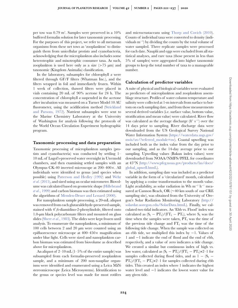
Fig. 1. Map of the CRE. Filled circle is the location of sampling.

Sample collection

Samples were collected in the third week of each monthduring 2005 and 2006 from a pier located at 46◦11′25′′N123◦49′28′′W, which is on the southern bank of theColumbia River in the city of Astoria, OR, ∼20 kmfrom the river mouth (Fig. 1). This pier extends ∼40 mfrom the shore, and at the point of collection water depthvaried between 4.0 and 6.5 m. This site experiences tidallyvariable intrusion of saline waters, which are either wellmixed or strongly stratified depending on hydrologicalconditions (Breckenridge et al., 2015).

On each sampling date, sampling was conducted dur-ing daylight hours. Temperature and salinity profiles wererecorded from the surface to the bottom using a YSI 85probe, and relative water clarity was estimated by mea-suring the Secchi depth. Surface water for microplank-ton (unicellular protists and cyanobacteria colonies ∼15–200 μm in size), nanoplankton (cells ∼5–15 μm in size),chlorophyll a and nutrient (NO3, NO2, PO4, SiO2) mea-surements was collected via triplicate bucket samples.Microplankton were collected in 200-mL water subsam-ples, preserved in 5% acid Lugols solution and storedin opaque jars until analysis. Nanoplankton subsampleswere collected in 100-mL opaque bottles, preserved ina 1% glutaraldehyde solution, then stained and filteredas described below, and frozen until analysis. In addi-tion, subsamples were taken for later laboratory analysesof chlorophyll a and nutrient concentrations. Metazoanplanktonic organisms ∼75 μm to 2 mm in size werecollected via triplicate vertical tows taken from 0.5 mabove the bottom to the surface with a 0.5-m diametermouth, 75-μm mesh net, with attached flowmeter (Gen-eral Oceanics Inc.). The average water volume sampled

223

Dow




per tow was 0.79 m3. Samples were preserved in a 10%buffered formalin solution for later taxonomic processing.For the purposes of this project, we refer to all metazoanorganisms from these net tows as ‘zooplankton’ to distin-guish them from unicellular protists and cyanobacteria,acknowledging that the microplankton also includes someheterotrophic and mixotrophic consumer taxa. As such,zooplankton is used here only as a size (>75 μm) andtaxonomic (Kingdom Animalia) classification.

In the laboratory, subsamples for chlorophyll a werefiltered through GF/F filters (Whatman Inc.), and thefilters wrapped in foil and immediately frozen. Within1 week of collection, thawed filters were placed invials containing 20 mL of 90% acetone for 24 h. Theconcentration of chlorophyll a suspended in the acetoneafter incubation was measured on a Turner Model 10 AUfluorometer, using the acidification method (Stricklandand Parsons, 1972). Nutrient subsamples were sent tothe Marine Chemistry Laboratory at the Universityof Washington for analysis following the protocols ofthe World Ocean Circulation Experiment hydrographicprogram.

Taxonomic processing and data preparation

Taxonomic processing of microplankton samples (pro-tists and cyanobacteria) was conducted by settling 1–10 mL of Lugol’s-preserved water overnight in Utermohlchambers, and then examining settled samples with anOlympus CK-40 inverted microscope at 200–400×. Allindividuals were identified to genus (and species whenpossible) using Patterson and Hedley (1992) and Wehret al. (2015), and sized using an ocular micrometer. Biovol-ume was calculated based on geometric shape (Hillebrandet al., 1999) and carbon biomass was then estimated usingthe algorithms of Menden-Deuer and Lessard (2000).

For nanoplankton sample processing, a 20-mL aliquotwas removed from each glutaraldehyde-preserved sample,stained with 4′,6-diamidino-2-phenylindole, filtered onto1.0-μm black polycarbonate filters and mounted on glassslides (Sherr et al., 1983). The slides were kept frozen untilanalysis. To enumerate the nanoplankton, a minimum of100 cells between 2 and 20 μm were counted using anepifluorescence microscope at 400–450× magnificationunder blue light. Cells were sized and nanoplankton car-bon biomass was estimated from biovolume as describedabove for microplankton.

An aliquot of 2–10 mL (1–5% of the entire sample) wassubsampled from each formalin-preserved zooplanktonsample, and a minimum of 200 non-naupliar organ-isms were identified and enumerated using a Leica MZ6stereomicroscope (Leica Microsystems). Identification tothe genus or species level was made for most rotifers

and microcrustaceans using Thorp and Covich (2010).Counts of individual taxa were converted to density (indi-viduals m−3) by dividing the counts by the total volume ofwater sampled. Three replicate samples were processedfor each date. Nauplii and eggs were excluded from all sta-tistical analyses, and rare taxa (those present in less than5% of samples) were aggregated into higher taxonomicgroups to keep the total number of taxa to a manageablenumber.

Calculation of predictor variables

A suite of physical and biological variables were evaluatedas predictors of microplankton and zooplankton assem-blage structure. Profiles of water column temperature andsalinity were collected at 1-m intervals from surface to bot-tom on each sampling date, and from those measurementsseveral derived variables (i.e. surface value, bottom value,stratification and mean value) were calculated. River flowwas calculated as the average discharge (ft3 s−1) over the14 days prior to sampling. River discharge data weredownloaded from the US Geological Survey NationalWater Information System (https://waterdata.usgs.gov/nwis/uv/?referred_module=sw). Coastal upwelling wasincluded both as the index value from the day prior toour sampling, and as the 14-day average prior to oursampling. Upwelling values (Bakun index values) weredownloaded from NOAA/NMFS/PFEL for coordinatesat 45◦N (http://www.pfeg.noaa.gov/products/las/docs/global_upwell.htmL).

In addition, sampling date was included as a predictorvariable in the form of a ‘circularized’ month, calculatedby applying a cosine transformation to the month value.Light availability, as solar radiation in Wh m−2 h−1 mea-sured at Cannon Beach, OR (∼40 km south of our CREsampling site), was obtained from the University of Ore-gon’s Solar Radiation Monitoring Laboratory (http://solardat.uoregon.edu/SolarData.htmL). Finally, we cal-culated two tidal indicators. An ‘Ebb vs. Flood’ index wascalculated as (St − PTt)/(FTt − PTt), where St was thetime when the samples were taken, PTt was the time ofthe previous tide change and FTt was the time of thefollowing tide change. When the sample was collected onan ebb tide, we multiplied this index by −1. Values of1 and −1 indicate the end of flood and the end of ebb,respectively, and a value of zero indicates a tide change.We created a similar but continuous index of high vs.low water, calculated as (St − PTt)/(FTt − PTt)∗2–1 forsamples collected during flood tides, and as 1 − (St −PTt)/(FTt − PTt)∗2–1 for samples collected during ebbtides. This created an index where 1 indicates the highestwater level and −1 indicates the lowest water value forany given tide.

224

Dow



https://waterdata.usgs.gov/nwis/uv/?referred_module=sw

https://waterdata.usgs.gov/nwis/uv/?referred_module=sw

http://www.pfeg.noaa.gov/products/las/docs/global_upwell.htmL

http://www.pfeg.noaa.gov/products/las/docs/global_upwell.htmL

http://solardat.uoregon.edu/SolarData.htmL

http://solardat.uoregon.edu/SolarData.htmL


Biological predictors of community compositionincluded water column chlorophyll a concentration,nanoplankton biomass and abundances or biomass ofhigher order taxonomic groupings of microplankton andzooplankton. Microplankton predictors of zooplanktonassemblage structure included the biomass of dinoflag-ellates, flagellates, ciliates, diatoms, chlorophytes andfilamentous bacteria. Diatoms were further divided intosize classes of 5–19, 20–49, 50–149 and >150 μm.Zooplankton predictors of microplankton assemblagestructure included the Log10 (x + 1) abundances ofrotifers, cladocerans, amphipods, calanoid copepods,harpacticoid copepods, cyclopoid copepods, total cope-pod nauplii, total copepodites, total adult copepodsand total zooplankton. Note that we also examinedmicroplankton predictors calculated as the Log10 (x + 1)abundances of these categories when testing the associa-tions of zooplankton assemblages with biotic and abioticfactors. However, the results did not differ substantivelyfrom those using microplankton predictors as biomass.Thus, we only report associations with zooplanktonassemblages using microplankton biomass, as these maybetter reflect the energy and material pathways throughthe lower planktonic food web.

Statistical analyses

We conducted a suite of non-parametric statisticalanalyses of community data following the generalstrategy outlined by Field et al. (1982) and Clarke (1993).This approach is largely robust to the temporal auto-correlation inherent in time-series data, and does notassume linearity of relationships or normality of data.Our approach consisted of non-metric multidimensionalscaling (NMDS), hierarchical agglomerative clusteringand correlating environmental vectors across ordinationspace. We also tested for significant (P < 0.05) differ-ences in biodiversity (calculated as Shannon’s H) andabundance or biomass among clusters via Kruskal–Wallis one-way ANOVA on ranks. Statistical analyseswere performed separately for the microplankton andzooplankton assemblages.

Ordination of assemblage data was conducted throughNMDS (Kruskal, 1964) of untransformed abundances for80 (microplankton) and 60 taxa (zooplankton). Both ordi-nations were constructed using the Bray–Curtis measureof dissimilarity, with ties in the dissimilarity matrix treatedaccording to Kruskal’s primary approach (no penalties forties). NMDS structure and dimensionality were validatedvia the examination of Shepard plots, and the Dexter et al.(2018) permutation test, which tests a null hypothesis thatobserved NMDS stress values could arise from stochasticsampling effects rather than strong species associations.

Hierarchical agglomerative clustering of assemblage datawas conducted using the flexible beta clustering algorithm(Kaufman and Rousseeuw, 1990) operating upon theBray–Curtis measure of dissimilarity. Values of beta forthe clustering algorithm were set to 0.6 for zooplanktonas well as microplankton data (Milligan, 1989).

The strength of correlation between environmentalpredictor variables and NMDS ordination scores wasassessed via the ‘ordisurf ’ function, which allows for non-linear correlations based upon a generalized additivemodel with penalized splines (Wood, 2003). For all ordina-tions, sufficiently linear predictor variables were overlainas arrows indicating the direction and strength of cor-relation with ordination axes, generated via the ‘envfit’function and assessed through permutation testing. Pre-dictor variables with strongly non-linear correlations werevisualized as topographic isoclines on separate ordinationplots, and are provided in the supplemental figures. Allmultivariate analyses were conducted using the veganpackage (Oksanen et al., 2017) for R version 3.2.2 (R CoreTeam, 2015).

RESULTS

Environmental conditions

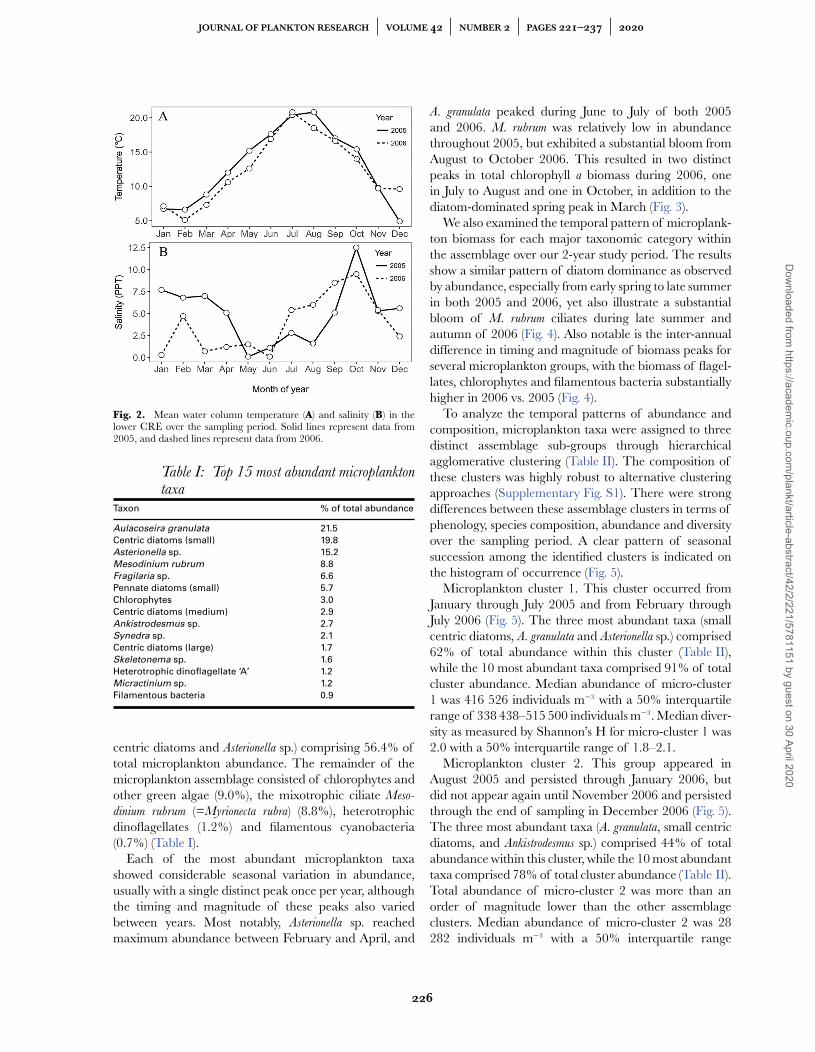
There were substantial seasonal and inter-annual differ-ences in the environmental conditions of the CRE duringour study period from January 2005 to December 2006.Water column temperatures were consistently highest insummer/autumn and lowest in winter of both years;however, waters were generally ∼2◦C warmer duringeach month in 2005 compared to 2006. Also, the periodof warmest temperatures (>15◦C) was longer in 2005(May–October) than in 2006 (June–September) (Fig. 2A).Seasonal and inter-annual differences in water columnsalinity were also pronounced. During 2005, salinity was>5 throughout the winter (January–April), then was <3throughout the late spring and summer, followed by apulse of high salinity (12) in October. In 2006, the sea-sonal pattern was nearly reversed: salinity was mostly <2during the winter and early spring (January–June), and>5 from July to November, with a high salinity pulse of9–10 during September–October (Fig. 2B).

MicroplanktonComposition and phenology of microplankton assemblages

Across our 2-year study period, the overall abundance ofthe microplankton assemblage was dominated by diatoms(75% of the abundance on average), with the threemost abundant diatom taxa (Aulacoseira granulata, small

225

Dow




Fig. 2. Mean water column temperature (A) and salinity (B) in thelower CRE over the sampling period. Solid lines represent data from2005, and dashed lines represent data from 2006.

Table I: Top 15 most abundant microplanktontaxa

Taxon % of total abundance

Aulacoseira granulata 21.5

Centric diatoms (small) 19.8

Asterionella sp. 15.2

Mesodinium rubrum 8.8

Fragilaria sp. 6.6

Pennate diatoms (small) 5.7

Chlorophytes 3.0

Centric diatoms (medium) 2.9

Ankistrodesmus sp. 2.7

Synedra sp. 2.1

Centric diatoms (large) 1.7

Skeletonema sp. 1.6

Heterotrophic dinoflagellate ‘A’ 1.2

Micractinium sp. 1.2

Filamentous bacteria 0.9

centric diatoms and Asterionella sp.) comprising 56.4% oftotal microplankton abundance. The remainder of themicroplankton assemblage consisted of chlorophytes andother green algae (9.0%), the mixotrophic ciliate Meso-

dinium rubrum (=Myrionecta rubra) (8.8%), heterotrophicdinoflagellates (1.2%) and filamentous cyanobacteria(0.7%) (Table I).

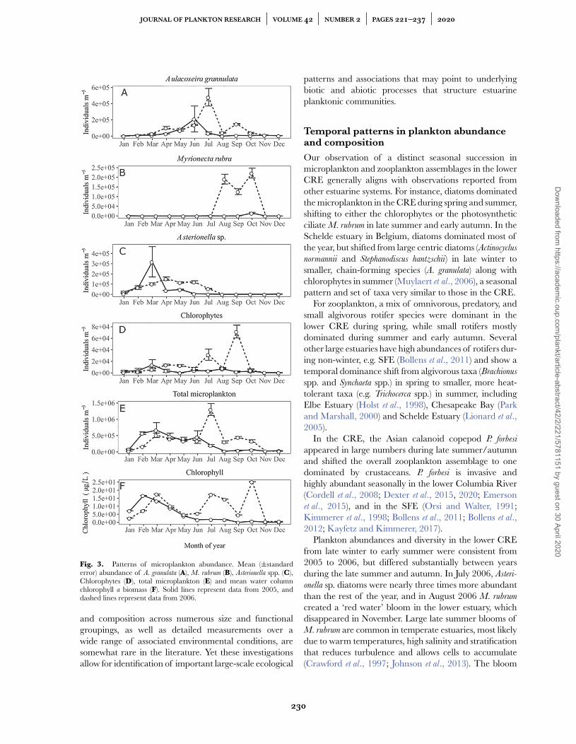
Each of the most abundant microplankton taxashowed considerable seasonal variation in abundance,usually with a single distinct peak once per year, althoughthe timing and magnitude of these peaks also variedbetween years. Most notably, Asterionella sp. reachedmaximum abundance between February and April, and

A. granulata peaked during June to July of both 2005and 2006. M. rubrum was relatively low in abundancethroughout 2005, but exhibited a substantial bloom fromAugust to October 2006. This resulted in two distinctpeaks in total chlorophyll a biomass during 2006, onein July to August and one in October, in addition to thediatom-dominated spring peak in March (Fig. 3).

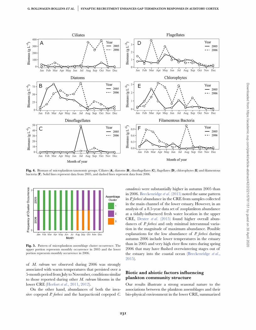
We also examined the temporal pattern of microplank-ton biomass for each major taxonomic category withinthe assemblage over our 2-year study period. The resultsshow a similar pattern of diatom dominance as observedby abundance, especially from early spring to late summerin both 2005 and 2006, yet also illustrate a substantialbloom of M. rubrum ciliates during late summer andautumn of 2006 (Fig. 4). Also notable is the inter-annualdifference in timing and magnitude of biomass peaks forseveral microplankton groups, with the biomass of flagel-lates, chlorophytes and filamentous bacteria substantiallyhigher in 2006 vs. 2005 (Fig. 4).

To analyze the temporal patterns of abundance andcomposition, microplankton taxa were assigned to threedistinct assemblage sub-groups through hierarchicalagglomerative clustering (Table II). The composition ofthese clusters was highly robust to alternative clusteringapproaches (Supplementary Fig. S1). There were strongdifferences between these assemblage clusters in terms ofphenology, species composition, abundance and diversityover the sampling period. A clear pattern of seasonalsuccession among the identified clusters is indicated onthe histogram of occurrence (Fig. 5).

Microplankton cluster 1. This cluster occurred fromJanuary through July 2005 and from February throughJuly 2006 (Fig. 5). The three most abundant taxa (smallcentric diatoms, A. granulata and Asterionella sp.) comprised62% of total abundance within this cluster (Table II),while the 10 most abundant taxa comprised 91% of totalcluster abundance. Median abundance of micro-cluster1 was 416 526 individuals m−3 with a 50% interquartilerange of 338 438–515 500 individuals m−3. Median diver-sity as measured by Shannon’s H for micro-cluster 1 was2.0 with a 50% interquartile range of 1.8–2.1.

Microplankton cluster 2. This group appeared inAugust 2005 and persisted through January 2006, butdid not appear again until November 2006 and persistedthrough the end of sampling in December 2006 (Fig. 5).The three most abundant taxa (A. granulata, small centricdiatoms, and Ankistrodesmus sp.) comprised 44% of totalabundance within this cluster, while the 10 most abundanttaxa comprised 78% of total cluster abundance (Table II).Total abundance of micro-cluster 2 was more than anorder of magnitude lower than the other assemblageclusters. Median abundance of micro-cluster 2 was 28282 individuals m−3 with a 50% interquartile range

226

Dow




Table II: The top 10 most abundant taxa for each of the microplankton assemblage clusters

Micro-cluster 1 % of total

abundance


abundance


abundance

Centric diatoms (small) 22.8 Aulacoseira granulata 18.5 Mesodinium rubrum 49.6

Aulacoseira granulata 20.5 Centric diatoms (small) 15.0 Aulacoseira granulata 21.3

Asterionella sp. 18.9 Ankistrodesmus sp. 10.7 Chlorophytes 7.8

Fragilaria sp. 8.5 Fragilaria sp. 8.2 Heterotrophic dinoflagellate

‘A’

5.7

Pennate diatoms (small) 7.8 Mesodinium rubrum 5.6 Ankistrodesmus sp. 3.4

Centric diatoms (medium) 3.7 Chlorophytes 5.2 Centric diatoms (small) 1.4

Synedra sp. 2.4 Heterotrophic dinoflagellate

‘A’

4.5 Amphora sp. 1.4

Ankistrodesmus sp. 2.3 Asterionella sp. 4.0 Filamentous bacteria 1.2

Skeletonema sp. 2.3 Centric diatoms (large) 3.3 Pennate diatoms (small) 1.2

Centric diatoms (large) 2.1 Pennate diatoms (small) 3.2 Fragilaria sp. 0.8

of 25 361–41 736 individuals m−3. Median diversityas measured by Shannon’s H for micro-cluster 2 wassignificantly higher than the other clusters, at 2.4 with a50% interquartile range of 2.3–2.7.

Microplankton cluster 3. Micro-cluster 3 was observedonly from August to October 2005 (Fig. 5). This clus-ter was dominated by a very large abundance of thebloom-forming mixotrophic ciliate M. rubrum, account-ing for 49.6% of the total abundance for this cluster.The three most abundant taxa in micro-cluster 3 (M.

rubrum, A. granulata and chlorophytes) comprised 79%of total abundance, while the 10 most abundant taxacomprised 94% of total cluster abundance (Table II).Total abundance of micro-cluster 3 was the same orderof magnitude as micro-cluster 1. Median abundanceof assemblage micro-cluster 3 was 332 969 individu-als m−3 with a 50% interquartile range of 319 712–389 873 individuals m−3. Median diversity as measuredby Shannon’s H for micro-cluster 3 was significantly lowerthan either of the other microplankton clusters, at 1.6with a 50% interquartile range of 1.5–2.7 (X 2 = 12.4,df = 2, P = 0.002). There were also significant differencesin total abundance between clusters (X 2 = 15.7, df = 2,P = 3.4 × 10−4).

Environmental correlates with the microplankton assemblage

A 2D NMDS ordination of the microplankton assem-blage data resulted in a stress value of 0.07, and the threemicroplankton clusters were plotted as an interpretiveoverlay on the NMDS ordination (Fig. 6). Results from1000 independent permutations of the microplanktonassemblage matrix using the Dexter et al. (2018) permu-tation test allowed us to reject the hypothesis that theobserved stress value of 0.07 could arise from stochasticsampling effects (z = −17.3; P < 0.001).

Strong correlations were observed between ordina-tion structure and several biological factors (rotifers,

cyclopoids and chlorophyll), physical factors (month,light, river flow, salinity and temperature) and chemicalfactors (phosphorus). These environmental correlates areplotted as vectors on the ordination of microplanktonassemblage data (Fig. 6). Salinity and river flow showeda strong but highly non-linear correlation and thusare visualized as topographic isoclines in separateplots (Supplementary Figs S2 and S3). In general, highflow/low salinity conditions were strongly associated withmicro-cluster 1, which strongly contrasts with the lowflow/high salinity regime associated with micro-clusters2 and 3.

A complete listing of the environmental variables sig-nificantly correlated with microplankton taxa, and theirassociation scores, is presented in Table III. In general,points situated on the right side of the NMDS ordi-nation (micro-clusters 1 and 3; Fig. 7) were associatedwith increasing abundances of cyclopoid copepods androtifers, elevated chlorophyll concentrations, and, to alesser extent, increasing light levels. Points situated onthe left side of the ordination (micro-cluster 2; Fig. 6) areassociated with increasing concentrations of phosphorus.The spread of points along ordination axis 2 is associatedwith seasonal environmental changes (i.e. temperatureand light availability).

ZooplanktonComposition and phenology of the zooplankton assemblage

Across the period of our study, the three most abundantzooplankton taxa were copepod nauplii, small unidenti-fied rotifers and Asplanchna spp. (Rotifera). These threetaxa comprised 74.2% of all zooplankton abundance,while the remainder of the zooplankton assemblage con-sisted of a relatively diverse set of copepod, cladoceranand rotifer taxa (Table IV). Of particular note, the inva-sive calanoid copepod, Pseudodiaptomus forbesi, comprised4.0% of total abundance.

227

Dow




Table III: Environmental correlates of microplankton ordination scores. These were assessed via the‘ordisurf ’ function in the R package ‘vegan,’ which allows for non-linear correlations based upon ageneralized additive model with penalized splines

Variable Deviance

explained (%)

F statistic Estimated deg.

of freedom

Uncorrected

P-value

Corrected

P-value

Salinity (mean) 81.2 6.55 7.6 8.0E-05 0.002∗Light 67.8 3.74 4.7 2.1E-04 0.002∗Chlorophyll 72.9 4.42 6.0 2.9E-04 0.002∗Cyclopoid copepods 63.9 3.21 4.3 3.3E-04 0.002∗Rotifera 63.8 3.20 4.3 3.4E-04 0.002∗Month (circularized) 68.1 3.65 5.2 4.4E-04 0.002∗Phosphorus 60.5 2.73 4.2 0.001 0.004∗Temperature (mean) 66.1 3.24 5.3 0.001 0.004∗River flow 68.3 3.25 6.4 0.004 0.011∗Nitrogen 33.1 0.99 1.6 0.012 0.031∗Upwelling 34.3 1.00 2.0 0.014 0.034∗Zooplankton 29.7 0.83 1.6 0.019 0.043∗Nanoplankton biomass 39.6 1.12 3.0 0.021 0.044∗Cladocera 35.4 0.95 2.6 0.023 0.046∗Copepod nauplii 27.3 0.72 1.5 0.027 0.047∗Calanoid copepods 27.0 0.71 1.5 0.029 0.047∗Copepodites 22.5 0.54 1.4 0.051 0.073

Silica 31.2 0.72 2.7 0.073 0.100

Asterisks indicate P-value < 0.05.

Table IV: Top 15 most abundant zooplanktontaxa from 2005 to 2006

Taxon % of total abundance

Copepod nauplii 40.7

Small unidentified rotifers 22.0

Asplanchna spp. 11.5

Coullana canadensis 4.1

Pseudodiaptomus forbesi 4.0

Keratella spp. 3.4

Eurytemora affinis 3.0

Polychaete larvae 2.7

Brachionus spp. 2.3

Cirripedia larvae 1.8

Bosmina longirostris 0.9

Polyarthra spp. 0.8

Pseudobradya spp. 0.5

Kellicottia spp. 0.4

Diacyclops thomasi 0.3

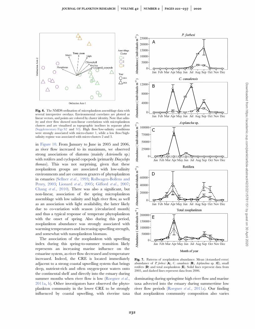
As observed in the microplankton assemblage, theabundances of many zooplankton taxa were highly vari-able seasonally and between years (Fig. 7). For instance, P.

forbesi showed a distinct peak in August and September ofboth years, and the abundance was more than seven timeshigher in 2005 (Fig. 7A). Similarly, the abundance of theharpacticoid copepod Coullana canadensis was somewhathigher in autumn 2006 than the rest of that year, butspiked upward by as much as 10-fold during three differ-ent months in 2005 (Fig. 7B). Asplanchna spp. abundancewas generally low during 2005, but peaked sharply inApril 2005 (Fig. 7C).

Hierarchical agglomerative clustering of zooplanktondata defined two assemblage clusters that differed with

respect to phenology, total abundance and species com-position.

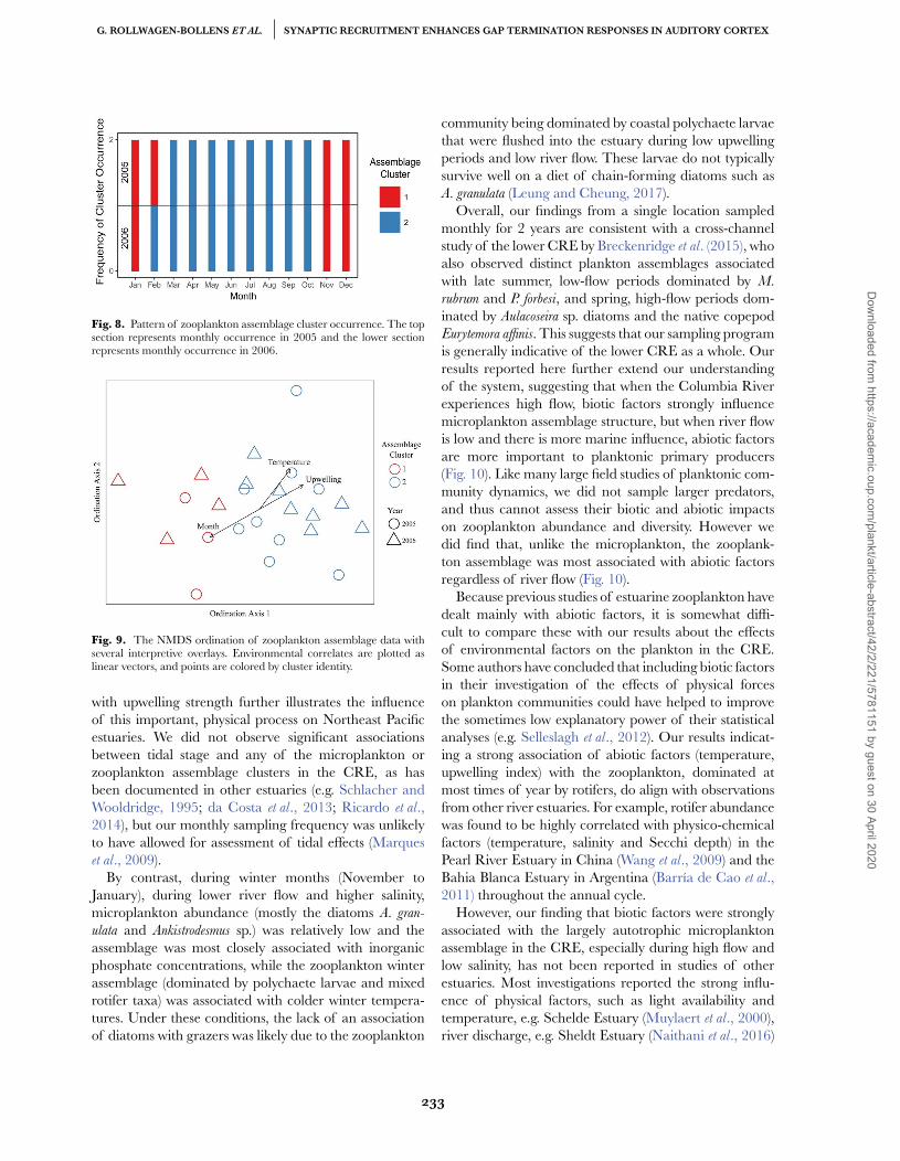
Zooplankton cluster 1. This cluster was observed inJanuary and February 2005 and again from November2005 to January 2006. This cluster was absent for9 months, and then re-emerged in November 2006(Fig. 8). The three most abundant taxa in zoop-cluster1 (Polychaete larvae, Rotifera and Cirripedia larvae)comprised 81% of total abundance within this group,while the 10 most abundant taxa comprised 94% of totalzoop-cluster abundance (Table V). Within zoop-cluster1, median abundance was 2 137 individuals m−3 with a50% interquartile range of 1 489–3 536 individuals m−3.Median diversity as measured by Shannon’s H for group1 was 1.3 with a 50% interquartile range of 1.0–1.9.

Zooplankton cluster 2. Zoop-cluster 2 was presentduring March–October 2005, and from February toOctober 2006 (Fig. 8). Total abundance within zoop-cluster 2 was approximately an order of magnitudegreater than zoop-cluster 1. The three most abundanttaxa (Rotifera, Asplanchna spp. and C. canadensis) comprised65% of total abundance in this cluster, while the 10most abundant taxa comprised 94% of total zoop-clusterabundance (Table V). The invasive calanoid copepod P.

forbesi comprised 6.9% of total cluster abundance, but insome months (e.g. September 2005) comprised greaterthan 90% of total assemblage abundance. Within zoop-cluster 2, median abundance was 17 217 individualsm−3 with a 50% interquartile range of 11 040–32 149individuals m−3 (Fig. 10A). Median diversity as measuredby Shannon’s H for zoop-cluster 2 was 1.4 with a 50%

228

Dow




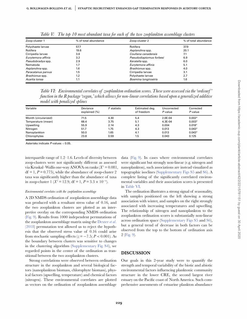
Table V: The top 10 most abundant taxa for each of the two zooplankton assemblage clusters

Zoop-cluster 1 % of total abundance Zoop-cluster 2 % of total abundance

Polychaete larvae 57.7 Rotifera 37.9

Rotifera 19.6 Asplanchna spp. 20.1

Cirripedia larvae 3.6 Coullana canadensis 7.1

Eurytemora affinis 3.2 Pseudodiaptomus forbesi 6.9

Pseudobradya spp. 2.9 Keratella spp. 6.0

Nematoda 1.7 Eurytemora affinis 5.1

Asplanchna spp. 1.6 Brachionus spp. 4.0

Paracalanus parvus 1.5 Cirripedia larvae 3.1

Brachionus spp. 1.2 Polychaete larvae 2.7

Acartia tonsa 1.1 Bosmina longirostris 1.6

Table VI: Environmental correlates of zooplankton ordination scores. These were assessed via the ‘ordisurf ’function in the R package ‘vegan,’ which allows for non-linear correlations based upon a generalized additivemodel with penalized splines

Variable Deviance

explained (%)

F statistic Estimated deg.

of freedom

Uncorrected

P-value

Corrected

P-value

Month (circularized) 71.5 4.30 5.4 2.0E-04 0.002∗Temperature (mean) 68.4 3.75 5.1 4.3E-04 0.003∗Upwelling 55.9 2.14 4.3 0.004 0.018∗Nitrogen 51.7 1.75 4.3 0.013 0.043∗Nanoplankton 50.0 1.65 4.1 0.013 0.043∗Chlorophytes 23.8 0.59 1.5 0.043 0.125

Asterisks indicate P-values < 0.05.

interquartile range of 1.2–1.6. Levels of diversity betweenzoop-clusters were not significantly different as assessedvia Kruskal–Wallis one-way ANOVA on ranks (X 2 = 0.081,df = 1, P = 0.775), while the abundance of zoop-cluster 2taxa was significantly higher than the abundance of taxain zoop-cluster 1 (X 2 = 12.9, df = 1, P = 3.3 × 10−4).

Environmental correlates with the zooplankton assemblage

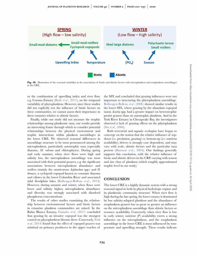
A 2D NMDS ordination of zooplankton assemblage datawas produced with a resultant stress value of 0.16, andthe two zooplankton clusters are plotted as an inter-pretive overlay on the corresponding NMDS ordination(Fig. 9). Results from 1000 independent permutations ofthe zooplankton assemblage matrix using the Dexter et al.(2018) permutation test allowed us to reject the hypoth-esis that the observed stress value of 0.16 could arisefrom stochastic sampling effects (z = −7.5; P < 0.001). Asthe boundary between clusters was sensitive to changesin the clustering algorithm (Supplementary Fig. S4), weregarded points in the center of the ordination as tran-sitional between the two zooplankton clusters.

Strong correlations were observed between ordinationstructure in the zooplankton and several biological fac-tors (nanoplankton biomass, chlorophyte biomass), phys-ical factors (upwelling, temperature) and chemical factors(nitrogen). These environmental correlates are plottedas vectors on the ordination of zooplankton assemblage

data (Fig. 9). In cases where environmental correlateswere significant but strongly non-linear (e.g. nitrogen andnanoplankton), such associations are instead visualized astopographic isoclines (Supplementary Figs S5 and S6). Acomplete listing of the significantly correlated environ-mental variables and their association scores is presentedin Table VI.

The ordination illustrates a strong signal of seasonality,with samples positioned on the left showing a strongassociation with winter, and samples on the right stronglyassociated with increasing temperatures and upwelling.The relationship of nitrogen and nanoplankton to thezooplankton ordination scores is substantially non-linearacross ordination space (Supplementary Figs S5 and S6),but a general trend of decrease in both factors can beobserved from the top to the bottom of ordination axis2 (Fig. 9).

DISCUSSION

Our goals in this 2-year study were to quantify thestrength and temporal variability of the biotic and abioticenvironmental factors influencing planktonic communitystructure in the lower CRE, the second largest riverestuary on the Pacific coast of North America. Such com-prehensive assessments of estuarine plankton abundance

229

Dow




Fig. 3. Patterns of microplankton abundance. Mean (±standarderror) abundance of A. granulata (A), M. rubrum (B), Asterionella spp. (C),Chlorophytes (D), total microplankton (E) and mean water columnchlorophyll a biomass (F). Solid lines represent data from 2005, anddashed lines represent data from 2006.

and composition across numerous size and functionalgroupings, as well as detailed measurements over awide range of associated environmental conditions, aresomewhat rare in the literature. Yet these investigationsallow for identification of important large-scale ecological

patterns and associations that may point to underlyingbiotic and abiotic processes that structure estuarineplanktonic communities.

Temporal patterns in plankton abundanceand composition

Our observation of a distinct seasonal succession inmicroplankton and zooplankton assemblages in the lowerCRE generally aligns with observations reported fromother estuarine systems. For instance, diatoms dominatedthe microplankton in the CRE during spring and summer,shifting to either the chlorophytes or the photosyntheticciliate M. rubrum in late summer and early autumn. In theSchelde estuary in Belgium, diatoms dominated most ofthe year, but shifted from large centric diatoms (Actinocyclus

normannii and Stephanodiscus hantzschii) in late winter tosmaller, chain-forming species (A. granulata) along withchlorophytes in summer (Muylaert et al., 2006), a seasonalpattern and set of taxa very similar to those in the CRE.

For zooplankton, a mix of omnivorous, predatory, andsmall algivorous rotifer species were dominant in thelower CRE during spring, while small rotifers mostlydominated during summer and early autumn. Severalother large estuaries have high abundances of rotifers dur-ing non-winter, e.g. SFE (Bollens et al., 2011) and show atemporal dominance shift from algivorous taxa (Brachionus

spp. and Synchaeta spp.) in spring to smaller, more heat-tolerant taxa (e.g. Trichocerca spp.) in summer, includingElbe Estuary (Holst et al., 1998), Chesapeake Bay (Parkand Marshall, 2000) and Schelde Estuary (Lionard et al.,2005).

In the CRE, the Asian calanoid copepod P. forbesi

appeared in large numbers during late summer/autumnand shifted the overall zooplankton assemblage to onedominated by crustaceans. P. forbesi is invasive andhighly abundant seasonally in the lower Columbia River(Cordell et al., 2008; Dexter et al., 2015, 2020; Emersonet al., 2015), and in the SFE (Orsi and Walter, 1991;Kimmerer et al., 1998; Bollens et al., 2011; Bollens et al.,2012; Kayfetz and Kimmerer, 2017).

Plankton abundances and diversity in the lower CREfrom late winter to early summer were consistent from2005 to 2006, but differed substantially between yearsduring the late summer and autumn. In July 2006, Asteri-

onella sp. diatoms were nearly three times more abundantthan the rest of the year, and in August 2006 M. rubrum

created a ‘red water’ bloom in the lower estuary, whichdisappeared in November. Large late summer blooms ofM. rubrum are common in temperate estuaries, most likelydue to warm temperatures, high salinity and stratificationthat reduces turbulence and allows cells to accumulate(Crawford et al., 1997; Johnson et al., 2013). The bloom

230

Dow




Fig. 4. Biomass of microplankton taxonomic groups. Ciliates (A), diatoms (B), dinoflagellates (C), flagellates (D), chlorophytes (E) and filamentousbacteria (F). Solid lines represent data from 2005, and dashed lines represent data from 2006.

Fig. 5. Pattern of microplankton assemblage cluster occurrence. Theupper portion represents monthly occurrence in 2005 and the lowerportion represents monthly occurrence in 2006.

of M. rubrum we observed during 2006 was stronglyassociated with warm temperatures that persisted over a5-month period from July to November, conditions similarto those reported during other M. rubrum blooms in thelower CRE (Herfort et al., 2011, 2012).

On the other hand, abundances of both the inva-sive copepod P. forbesi and the harpacticoid copepod C.

canadensis were substantially higher in autumn 2005 thanin 2006. Breckenridge et al. (2015) noted the same patternin P. forbesi abundance in the CRE from samples collectedin the main channel of the lower estuary. However, in ananalysis of a 8.5-year data set of zooplankton abundanceat a tidally-influenced fresh water location in the upperCRE, Dexter et al. (2015) found higher overall abun-dances of P. forbesi and only minimal interannual varia-tion in the magnitude of maximum abundance. Possibleexplanations for the low abundance of P. forbesi duringautumn 2006 include lower temperatures in the estuarythan in 2005 and very high river flow rates during spring2006 that may have flushed overwintering stages out ofthe estuary into the coastal ocean (Breckenridge et al.,2015).

Biotic and abiotic factors influencingplankton community structure

Our results illustrate a strong seasonal nature to theassociations between the plankton assemblages and theirbio-physical environment in the lower CRE, summarized

231

Dow




Fig. 6. The NMDS ordination of microplankton assemblage data withseveral interpretive overlays. Environmental correlates are plotted aslinear vectors, and points are colored by cluster identity. Note that salin-ity and river flow showed non-linear correlations with microplanktonclusters and are visualized as topographic isoclines in separate plots(Supplementary Figs S2 and S3). High flow/low-salinity conditionswere strongly associated with micro-cluster 1, while a low flow/high-salinity regime was associated with micro-clusters 2 and 3.

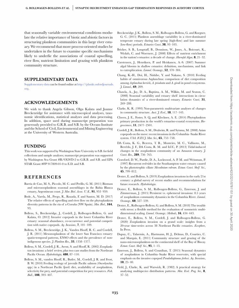
in Figure 10. From January to June in 2005 and 2006,as river flow increased to its maximum, we observedstrong associations of diatoms (mainly Asterionella sp.)with rotifers and cyclopoid copepods (primarily Diacyclops

thomasi). This was not surprising, given that thesezooplankton groups are associated with low-salinityenvironments and are common grazers of phytoplanktonin estuaries (Sellner et al., 1993; Rollwagen-Bollens andPenry, 2003; Lionard et al., 2005; Gifford et al., 2007;Chang et al., 2010). There was also a significant, butnon-linear, association of the spring microplanktonassemblage with low salinity and high river flow, as wellas an association with light availability, the latter likelydue to co-variation with season (circularized month)and thus a typical response of temperate phytoplanktonwith the onset of spring. Also during this period,zooplankton abundance was strongly associated withwarming temperatures and increasing upwelling strength,and somewhat with nanoplankton biomass.

The association of the zooplankton with upwellingindex during this spring-to-summer transition likelyrepresents an increasing marine influence on theestuarine system, as river flow decreased and temperatureincreased. Indeed, the CRE is located immediatelyadjacent to a strong coastal upwelling system that bringsdeep, nutrient-rich and often oxygen-poor waters ontothe continental shelf and directly into the estuary duringsummer months when river flow is low (Roegner et al.,2011a, b). Other investigators have observed the phyto-plankton community in the lower CRE to be stronglyinfluenced by coastal upwelling, with riverine taxa

Fig. 7. Patterns of zooplankton abundance. Mean (±standard error)abundance of P. forbesi (A), C. canadensis (B), Asplanchna sp. (C), smallrotifers (D) and total zooplankton (E). Solid lines represent data from2005, and dashed lines represent data from 2006.

dominating during springtime high river flow and marinetaxa advected into the estuary during summertime lowriver flow periods (Roegner et al., 2011a). Our findingthat zooplankton community composition also varies

232

Dow




Fig. 8. Pattern of zooplankton assemblage cluster occurrence. The topsection represents monthly occurrence in 2005 and the lower sectionrepresents monthly occurrence in 2006.

Fig. 9. The NMDS ordination of zooplankton assemblage data withseveral interpretive overlays. Environmental correlates are plotted aslinear vectors, and points are colored by cluster identity.

with upwelling strength further illustrates the influenceof this important, physical process on Northeast Pacificestuaries. We did not observe significant associationsbetween tidal stage and any of the microplankton orzooplankton assemblage clusters in the CRE, as hasbeen documented in other estuaries (e.g. Schlacher andWooldridge, 1995; da Costa et al., 2013; Ricardo et al.,2014), but our monthly sampling frequency was unlikelyto have allowed for assessment of tidal effects (Marqueset al., 2009).

By contrast, during winter months (November toJanuary), during lower river flow and higher salinity,microplankton abundance (mostly the diatoms A. gran-

ulata and Ankistrodesmus sp.) was relatively low and theassemblage was most closely associated with inorganicphosphate concentrations, while the zooplankton winterassemblage (dominated by polychaete larvae and mixedrotifer taxa) was associated with colder winter tempera-tures. Under these conditions, the lack of an associationof diatoms with grazers was likely due to the zooplankton

community being dominated by coastal polychaete larvaethat were flushed into the estuary during low upwellingperiods and low river flow. These larvae do not typicallysurvive well on a diet of chain-forming diatoms such asA. granulata (Leung and Cheung, 2017).

Overall, our findings from a single location sampledmonthly for 2 years are consistent with a cross-channelstudy of the lower CRE by Breckenridge et al. (2015), whoalso observed distinct plankton assemblages associatedwith late summer, low-flow periods dominated by M.

rubrum and P. forbesi, and spring, high-flow periods dom-inated by Aulacoseira sp. diatoms and the native copepodEurytemora affinis. This suggests that our sampling programis generally indicative of the lower CRE as a whole. Ourresults reported here further extend our understandingof the system, suggesting that when the Columbia Riverexperiences high flow, biotic factors strongly influencemicroplankton assemblage structure, but when river flowis low and there is more marine influence, abiotic factorsare more important to planktonic primary producers(Fig. 10). Like many large field studies of planktonic com-munity dynamics, we did not sample larger predators,and thus cannot assess their biotic and abiotic impactson zooplankton abundance and diversity. However wedid find that, unlike the microplankton, the zooplank-ton assemblage was most associated with abiotic factorsregardless of river flow (Fig. 10).

Because previous studies of estuarine zooplankton havedealt mainly with abiotic factors, it is somewhat diffi-cult to compare these with our results about the effectsof environmental factors on the plankton in the CRE.Some authors have concluded that including biotic factorsin their investigation of the effects of physical forceson plankton communities could have helped to improvethe sometimes low explanatory power of their statisticalanalyses (e.g. Selleslagh et al., 2012). Our results indicat-ing a strong association of abiotic factors (temperature,upwelling index) with the zooplankton, dominated atmost times of year by rotifers, do align with observationsfrom other river estuaries. For example, rotifer abundancewas found to be highly correlated with physico-chemicalfactors (temperature, salinity and Secchi depth) in thePearl River Estuary in China (Wang et al., 2009) and theBahia Blanca Estuary in Argentina (Barría de Cao et al.,2011) throughout the annual cycle.

However, our finding that biotic factors were stronglyassociated with the largely autotrophic microplanktonassemblage in the CRE, especially during high flow andlow salinity, has not been reported in studies of otherestuaries. Most investigations reported the strong influ-ence of physical factors, such as light availability andtemperature, e.g. Schelde Estuary (Muylaert et al., 2000),river discharge, e.g. Sheldt Estuary (Naithani et al., 2016)

233

Dow




Fig. 10. Illustration of the seasonal variability in the associations of biotic and abiotic factors with microplankton and zooplankton assemblagesin the CRE.

or the combination of upwelling index and river flow,e.g. Coruna Estuary (Bode et al., 2017), on the temporalvariability of phytoplankton. However, since these studiesdid not explicitly test the influence of biotic factors onthese communities, we cannot assess their importance inthese estuaries relative to abiotic factors.

Finally, while our study did not measure the trophicrelationships among planktonic taxa, our results providean interesting frame through which to consider potentialrelationships between the physical environment andtrophic interactions within plankton assemblages inthe lower CRE. We observed seasonal differences inassemblage structure to be most pronounced among themicroplankton, particularly autotrophic taxa (especiallydiatoms, M. rubrum and chlorophytes). During springand early summer, when river flows were high andsalinity low, the microplankton assemblage was mostassociated with their potential grazers, e.g. the significantassociations between microplankton abundance androtifers (mainly the omnivorous Asplanchna spp.) and D.

thomasi, a cyclopoid copepod known to consume diatomsand ciliates in the lower Columbia River and associatedtidal floodplain lakes (Rollwagen-Bollens et al., 2013).However, during autumn and winter, when flows werelower and salinity higher, microplankton abundanceand diversity was strongly associated with dissolvedphosphorus concentrations.

The results of other studies examining the relation-ship between environmental factors and biotic factorsin estuarine plankton communities are mixed. In theBahia Blanca Estuary, Guinder et al. (2017) concludedthat grazing by an invasive copepod was the strongestcontrol on phytoplankton blooms there. Conversely, Yorket al. (2014) found that the effect of copepod grazers wasminimal on primary producers in the upper reaches of

the SFE and concluded that grazing influences were notimportant to structuring the phytoplankton assemblage.Rollwagen-Bollens et al. (2006) showed similar results inthe lower SFE, where grazing by the abundant copepodtaxon Acartia spp. had a greater impact on heterotrophicprotist grazers than on autotrophic plankton. And in theYork River Estuary in Chesapeake Bay, the investigatorsobserved a lack of grazing effects on the phytoplankton(Sin et al., 2006).

Both terrestrial and aquatic ecologists have begun toconverge on the notion that the relative influence of top-down (i.e. predation, grazing) vs. bottom-up (i.e. nutrientavailability) drivers is strongly case dependent, and mayvary with scale, abiotic factors and the particular taxapresent (Hansson et al., 2004). Our findings generallysupports this conclusion, with the relative influence ofbiotic and abiotic drivers in the CRE varying with seasonand size class of plankton (which roughly approximatedtrophic level in our study).

CONCLUSION

The lower CRE is a highly dynamic system with a strongseasonal signal in both its physical-hydrologic regime andits planktonic community structure. When river flow ishigh during the late spring, the lower estuary is dominatedby low salinity-adapted plankton and the abundance ofzooplankton grazers has as great or greater an influenceon the microplankton assemblage than abiotic factors orresource availability. Conversely, when river flow is lowin early winter, nutrient (P ) availability exerts a stronginfluence on the microplankton, and the zooplanktonassemblage in the lower CRE is most influenced by tem-perature and upwelling strength. These results indicate

234

Dow




that seasonally variable environmental conditions modu-late the relative importance of biotic and abiotic factors instructuring plankton communities in this large river estu-ary. We recommend that more process-oriented studies beundertaken in the future to examine specific mechanismslikely to underlie the associations of coastal upwelling,river flow, nutrient limitation and grazing with planktoncommunity structure.

SUPPLEMENTARY DATASupplementary data can be found online at http://plankt.oxfordjournals.org.

ACKNOWLEDGEMENTSWe wish to thank Angela Gibson, Olga Kalata and JoanneBreckenridge for assistance with microscopical analyses, taxo-nomic identifications, statistical analyses and data processing.In addition, space used during manuscript preparation wasgenerously provided to G.R.B. and S.B. by the Oceans Instituteand the School of Civil, Environmental and Mining Engineeringat the University of Western Australia.

FUNDINGThis work was supported by Washington State University to S.B. for fieldcollections and sample analyses; manuscript preparation was supportedby Washington Sea Grant #R/OLWD-2 to G.R.B. and S.B. and EPASTAR Grant #FP 917809-01-0 to E.D. and S.B.

R E F E R E N C E SBarría de Cao, M. S., Piccolo, M. C. and Perillo, G. M. (2011) Biomass

and microzooplankton seasonal assemblages in the Bahía Blancaestuary, Argentinean coast. J. Mar. Biol. Assoc. U. K., 91, 953–959.

Bode, A., Varela, M., Prego, R., Rozada, F. and Santos, M. D. (2017)The relative effects of upwelling and river flow on the phytoplanktondiversity patterns in the ria of a Coruña (NW Spain). Mar. Biol., 164,93.

Bollens, S., Breckenridge, J., Cordell, J., Rollwagen-Bollens, G. andKalata, O. (2012) Invasive copepods in the lower Columbia Riverestuary: seasonal abundance, co-occurrence and potential competi-tion with native copepods. Aq. Invasions, 7, 101–109.

Bollens, S. M., Breckenridge, J. K., Vanden Hooff, R. C. and Cordell,J. R. (2011) Mesozooplankton of the lower San Francisco estuary:spatio-temporal patterns, ENSO effects and the prevalence of non-indigenous species. J. Plankton Res., 33, 1358–1377.

Bollens, S. M., Cordell, J. R., Avent, S. and Hooff, R. (2002) Zooplank-ton invasions: a brief review, plus two case studies from the NortheastPacific Ocean. Hydrobiologia, 480, 87–110.

Bollens, S. M., vanden Hooff, R., Butler, M., Cordell, J. R. and Frost,B. W. (2010) Feeding ecology of juvenile Pacific salmon (Oncorhynchus

spp.) in a Northeast Pacific fjord: diet, availability of zooplankton,selectivity for prey, and potential competition for prey resources. Fish.

Bull., 108, 393–407.

Breckenridge, J. K., Bollens, S. M., Rollwagen-Bollens, G. and Roegner,G. C. (2015) Plankton assemblage variability in a river-dominatedtemperate estuary during late spring (high-flow) and late summer(low-flow) periods. Estuaries Coast, 38, 93–103.

Bricker, S. B., Longstaff, B., Dennison, W., Jones, A., Boicourt, K.,Wicksb, C. and Woernerc, J. (2008) Effects of nutrient enrichmentin the nation’s estuaries: a decade of change. Harmful Algae, 8, 21–32.

Carstensen, J., Henriksen, P. and Heiskanen, A.-S. (2007) Summeralgal blooms in shallow estuaries: definition, mechanisms, and linkto eutrophication. Limnol. Oceanogr., 52, 370–384.

Chang, K.-H., Doi, H., Nishibe, Y. and Nakano, S. (2010) Feedinghabits of omnivorous Asplanchna: comparison of diet compositionamong Asplanchna herricki, A. priodonta and A. girodi in pond ecosystems.J. Limnol., 69, 209.

Chawla, A., Jay, D. A., Baptista, A. M., Wilkin, M. and Seaton, C.(2008) Seasonal variability and estuary–shelf interactions in circu-lation dynamics of a river-dominated estuary. Estuaries Coast, 31,269–288.

Clarke, K. R. (1993) Non-parametric multivariate analyses of changesin community structure. Aust. J. Ecol., 18, 117–143.

Cloern, J. E., Foster, S. Q. and Kleckner, A. E. (2014) Phytoplanktonprimary production in the world’s estuarine-coastal ecosystems. Bio-

geosciences, 11, 2477–2501.

Cordell, J. R., Bollens, S. M., Draheim, R. and Sytsma, M. (2008) Asiancopepods on the move: recent invasions in the Columbia–Snake Riversystem. USA. ICES J. Mar. Sci., 65, 753–758.

DA Costa, K. G., Bezerra, T. R., Monteiro, M. C., Vallinoto, M.,Berrêdo, J. F., DA Costa, R. M. and LCC, P. (2013) Tidal-inducedchanges in the zooplankton community of an Amazon estuary. J.

Coast. Res., 289, 756–765.

Crawford, D. W., Purdie, D. A., Lockwood, A. P. M. and Weissman, P.(1997) Recurrent red-tides in the Southampton water estuary causedby the phototrophic ciliate Mesodinium rubrum. Estuar. Coast. Shelf Sci.,45, 799–812.

Dexter, E. and Bollens, S. (2019) Zooplankton invasions in the early 21stcentury: a global survey of recent studies and recommendations forfuture research. Hydrobiologia.

Dexter, E., Bollens, S. M., Rollwagen-Bollens, G., Emerson, J. andZimmerman, J. (2015) Persistent vs. ephemeral invasions: 8.5 yearsof zooplankton community dynamics in the Columbia River. Limnol.

Oceanogr., 60, 527–539.

Dexter, E., Rollwagen-Bollens, G. and Bollens, S. M. (2018) The troublewith stress: a flexible method for the evaluation of nonmetric multi-dimensional scaling. Limnol. Oceanogr.: Methods, 16, 434–443.

Dexter, E., Bollens, S. M., Cordell, J. and Rollwagen-Bollens, G.(2020) Zooplankton invasion on a grand scale: insights from a20-year time-series across 38 Northeast Pacific estuaries. Ecosphere,In Press.

Dupuy, C., Talarmin, A., Hartmann, H. J., Delmas, D., Courties, C.and Marquis, E. (2011) Community structure and grazing of thenano-microzooplankton on the continental shelf of the Bay of Biscay.Estuar. Coast. Shelf Sci., 95, 1–13.

Emerson, J., Bollens, S. and Counihan, T. (2015) Seasonal dynamicsof zooplankton in Columbia–Snake River reservoirs, with specialemphasis on the invasive copepod Pseudodiaptomus forbesi. Aq. Invasions,10, 25–40.

Field, J., Clarke, K. and Warwick, R. (1982) A practical strategy foranalysing multispecies distribution patterns. Mar. Ecol. Prog. Ser., 8,37–52.

235

Dow



https://academic.oup.com/plankt/article-lookup/doi/10.1093/plankt/fbaa010#supplementary-data

http://plankt.oxfordjournals.org

http://plankt.oxfordjournals.org


Gallegos, C. L., Jordan, T. E. and Hedrick, S. S. (2010) Long-termdynamics of phytoplankton in the Rhode River, Maryland (USA).Estuaries Coast, 33, 471–484.

Gifford, S., Rollwagen-Bollens, G. and Bollens, S. (2007) Mesozooplank-ton omnivory in the upper San Francisco estuary. Mar. Ecol. Prog. Ser.,348, 33–46.

Goertler, P. A. L., Simenstad, C. A., Bottom, D. L., Hinton, S. andStamatiou, L. (2016) Estuarine habitat and demographic factors affectjuvenile Chinook (Oncorhynchus tshawytscha) growth variability in a largefreshwater tidal estuary. Estuaries Coast, 39, 542–559.

Graham, E. S. and Bollens, S. M. (2010) Macrozooplankton communitydynamics in relation to environmental variables in Willapa Bay,Washington, USA. Estuaries Coast, 33, 182–194.

Guinder, V. A., Molinero, J. C., López Abbate, C. M., Berasategui, A.A., Popovich, C. A., Spetter, C., Morcovecchio, J. and Freije, H. (2017)Phenological changes of blooming diatoms promoted by compoundbottom-up and top-down controls. Estuaries Coast, 40, 95–104.

Haertel, L. and Osterberg, C. (1967) Ecology of zooplankton, benthosand fishes in the Columbia River estuary. Ecology, 48, 459–472.

Haertel, L., Osterberg, C., Curl, H. and Park, P. K. (1969) Nutrientand plankton ecology of the Columbia River estuary. Ecology, 50,962–978.

Hansson, L.-A., Gyllstrom, M., Stahl-Delbanco, A. and Svensson,M. (2004) Responses to fish predation and nutrients by plank-ton at different levels of taxonomic resolution. Freshwater Biol., 49,1538–1550.

Herfort, L., Peterson, T. D., Campbell, V., Futrell, S. and Zuber, P. (2011)Myrionecta rubra (Mesodinium rubrum) bloom initiation in the ColumbiaRiver estuary. Estuar. Coast. Shelf Sci., 95, 440–446.

Herfort, L., Peterson, T. D., Prahl, F. G., McCue, L. A., Needoba, J. A.,Crump, B., Reogner, G. C., Campbell, V. et al. (2012) Red waters ofMyrionecta rubra are biogeochemical hotspots for the Columbia Riverestuary with impacts on primary/secondary productions and nutrientcycles. Estuaries Coast, 35, 878–891.

Hickey, B. M., Pietrafesa, L. J., Jay, D. A. and Boicourt, W. C. (1998)The Columbia River plume study: subtidal variability in the velocityand salinity fields. J. Geophys. Res.: Oceans, 103, 10339–10368.

Hillebrand, H., Dürselen, C.-D., Kirschtel, D., Pollingher, U. andZohary, T. (1999) Biovolume calculation for pelagic and benthicmicroalgae. J. Phycol., 35, 403–424.

Holst, H., Zimmermann, H., Kausch, H. and Koste, W. (1998) Tem-poral and spatial dynamics of planktonic rotifers in the Elbe estuaryduring spring. Estuar. Coast. Shelf Sci., 47, 261–273.

Jay, D. A. and Smith, J. D. (1990) Circulation, density distribution andneap-spring transitions in the Columbia River estuary. Prog. Oceanogr.,25, 81–112.

Johnson, M. D., Stoecker, D. K. and Marshall, H. G. (2013) Seasonaldynamics of Mesodinium rubrum in Chesapeake Bay. J. Plankton Res.,35, 877–893.

Jones, K. K., Simenstad, C. A., Higley, D. L. and Bottom, D. L.(1990) Community structure, distribution, and standing stock ofbenthos, epibenthos, and plankton in the Columbia River estuary.Prog. Oceanogr., 25, 211–241.

Kaufman, L. and Rousseeuw, P. (1990) Finding Groups in Data: An Intro-

duction to Cluster Analysis, Wiley, Hoboken, NJ, USA.

Kayfetz, K. and Kimmerer, W. (2017) Abiotic and biotic controls onthe copepod Pseudodiaptomus forbesi in the upper San Francisco estuary.Mar. Ecol. Prog. Ser., 581, 85–101.

Keefer, M. L., Peery, C. A., Jepson, M. A., Tolotti, K. R., Bjornn, T.C. and Stuehrenberg, L. C. (2004) Stock-specific migration timing ofadult spring–summer Chinook salmon in the Columbia River basin.N. Amer. J. Fish. Manage., 24, 1145–1162.

Kennish, M. J. (2002) Environmental threats and environmental futureof estuaries. Environ. Conserv., 29, 78–107.

Kimmerer, W. J., Burau, J. R. and Bennett, W. A. (1998) Tidally orientedvertical migration and position maintenance of zooplankton in atemperate estuary. Limnol. Oceanogr., 43, 1697–1709.

Kirn, R. A., Ledgerwood, R. O. and Jensen, A. L. (1985) Diet of sub-yearling Chinook salmon (Oncorhynchus tshawytscha) in the ColumbiaRiver estuary and changes effected by the 1980 eruption of MountSt. Helens. Northwest Sci., 60, 191–196.

Kruskal, J. B. (1964) Multidimensional scaling by optimizing goodnessof fit to a nonmetric hypothesis. Psychometrika, 29, 1–27.

Laprise, R. and Dodson, J. J. (1994) Environmental variability as a factorcontrolling spatial patterns in distribution and species diversity ofzooplankton in the St. Lawrence estuary. Mar. Ecol. Prog. Ser., 107,67–81.

Leung, J. Y. S. and Cheung, N. K. M. (2017) Feeding behaviour of aserpulid polychaete: turning a nuisance species into a natural resourceto counter algal blooms? Mar. Pollut. Bull., 115, 376–382.

Lionard, M., Azémar, F., Boulêtreau, S., Muylaert, K., Tackx, M. andVyverman, W. (2005) Grazing by meso- and microzooplankton onphytoplankton in the upper reaches of the Schelde estuary (Bel-gium/the Netherlands). Estuar. Coast. Shelf Sci., 64, 764–774.

Marques, S. C., Azeiteiro, U. M., Martinho, F., Viegas, I. and Pardal,M. A. (2009) Evaluation of estuarine mesozooplankton dynamics ata fine temporal scale: the role of seasonal, lunar and diel cycles. J.

Plankton Res., 31, 1249–1263.

Martínez, M. L., Intralawan, A., Vázquez, G., Pérez-Maqueo, O., Sut-ton, P. and Landgrave, R. (2007) The coasts of our world: ecological,economic and social importance. Ecol. Econ., 63, 254–272.

Menden-Deuer, S. and Lessard, E. J. (2000) Carbon to volume relation-ships for dinoflagellates, diatoms, and other protist plankton. Limnol.

Oceanogr., 45, 569–579.

Milligan, G. (1989) A study of the beta-flexible clustering method.Multivar. Behav. Res., 24, 163–176.

Muylaert, K., Declerck, S., Van Wichelen, J., De Meester, L. and Vyver-man, W. (2006) An evaluation of the role of daphnids in controllingphytoplankton biomass in clear water versus turbid shallow lakes.Limnol - Ecol Manage Inland Waters, 36, 69–78.

Muylaert, K., Sabbe, K. and Vyverman, W. (2000) Spatial and temporaldynamics of phytoplankton communities in a freshwater tidal estuary(Schelde, Belgium). Estuar. Coast. Shelf Sci., 50, 673–687.

Naithani, J., DE Brye, B., Buyze, E., Vyverman, W., Legat, V. andDeleersnijder, E. (2016) An ecological model for the Scheldt estuaryand tidal rivers ecosystem: spatial and temporal variability of plank-ton. Hydrobiologia, 775, 51–67.

Neitzel, D., Page, T. and Hanf , R. (1982) Mid-Columbia Rivermicroflora. J. Freshwater Ecol., 1, 495–505.

Oksanen, J., Blanchet, F. G., Friendly, M., Kindt, R., Legendre, P.,Minchin, P. R., O’Hara, B., Simpson, G. L. et al. (2017) Vegan:community ecology package.

Orsi, J. J. and Walter, T. C. (1991) Pseudodiaptomus forbesi and P. marinus

(Copepoda Calanoida), the latest copepod immigrants to California’sSacramento - San Joaquin estuary. Bull. Plankton Soc. Japan, 1991,553–562.

236

Dow




Park, G. S. and Marshall, H. G. (2000) The trophic contributions ofrotifers in tidal freshwater and estuarine habitats. Estuar. Coast. Shelf

Sci., 51, 729–742.

Patterson, D. J. and Hedley, S. (1992) Free-Living Freshwater Protozoa: A

Colour Guide, Wolfe Publishing, Boca Raton, FL, USA.

Payne, J. T., Wood, A. W., Hamlet, A. F., Palmer, R. N. and Let-tenmaier, D. P. (2004) Mitigating the effects of climate change onthe water resources of the Columbia River basin. Clim. Change, 62,233–256.

R Core Team (2015) R: The R Project for Statistical Computing.

Ricardo, G. F., Davis, A. R., Knott, N. A. and Minchinton, T. E. (2014)Diel and tidal cycles regulate larval dynamics in salt marshes andmangrove forests. Mar. Biol., 161, 769–784.

Richardson, A. J. (2008) In hot water: zooplankton and climate change.ICES J. Mar. Sci., 65, 279–295.

Richardson, A. J. and Schoeman, D. S. (2004) Climate impact on plank-ton ecosystems in the Northeast Atlantic. Science, 305, 1609–1612.

Robins, P. E., Skov, M. W., Lewis, M. J., Giménez, L., Davies, A.G., Malham, S. K., Neill, S. P., JE, M. D. et al. (2016) Impact ofclimate change on UK estuaries: a review of past trends and potentialprojections. Estuar. Coast. Shelf Sci., 169, 119–135.

Roegner, G. C., Needoba, J. A. and Baptista, A. M. (2011a) Coastalupwelling supplies oxygen-depleted water to the Columbia Riverestuary. PLoS One, 6, e18672.

Roegner, G. C., Seaton, C. and Baptista, A. M. (2011b) Climatic andtidal forcing of hydrography and chlorophyll concentrations in theColumbia River estuary. Estuaries Coast, 34, 281–296.

Rollwagen-Bollens, G., Bollens, S., Gonzalez, A., Zimmerman, J., Lee,T. et al. (2013) Feeding dynamics of the copepod Diacyclops thomasi

before, during and following filamentous cyanobacteria blooms in alarge, shallow temperate lake. Hydrobiologia, 705, 101–118.

Rollwagen-Bollens, G. C., Bollens, S. M. and Penry, D. L. (2006) Verticaldistribution of micro-and nanoplankton in the San Francisco estuaryin relation to hydrography and predators. Aquat. Microb. Ecol., 44,143–163.

Rollwagen-Bollens, G. C. R. and Penry, D. L. (2003) Feeding dynamicsof Acartia spp. copepods in a large, temperate estuary (San FranciscoBay, CA). Mar. Ecol. Prog. Ser., 257, 139–158.

Roy, E. D., Smith, E. A., Bargu, S. and White, J. R. (2016) WillMississippi River diversions designed for coastal restoration causeharmful algal blooms? Ecol. Eng., 91, 350–364.

Schlacher, T. A. and Wooldridge, T. H. (1995) Small-scale distributionand variability of demersal zooplankton in a shallow, temperateestuary: tidal and depth effects on species-specific heterogeneity. Cah.

Biol. Mar., 36, 211–227.

Selleslagh, J., Lobry, J., N’Zigou, A. R., Bachelet, G., Blanchet, H.,Chaalali, A., Sautour, B. and Boët, P. (2012) Seasonal successionof estuarine fish, shrimps, macrozoobenthos and plankton: Physico-chemical and trophic influence. The Gironde estuary as a case study.Estuar. Coast. Shelf Sci., 112, 243–254.

Sellner, K. G., Brownlee, D. C., Bundy, M. H., Brownlee, S. G.and Braun, K. R. (1993) Zooplankton grazing in a Potomac Rivercyanobacteria bloom. Estuaries, 16, 859–872.

Sherr, E., Caron, D. and Sherr, B. (1983) Staining of heterotrophicprotists for visualization via epifluorescence microscopy. In Kemp, P.(ed.), Handbook of methods in Aquat. Microb. Ecol, Lewis Publishers, BocaRaton, pp. 213–227.

Simenstad, C., Small, L., McIntire, C., Jay, D. and Sherwood, C. (1990a)Columbia River estuary studies - an introduction to the estuary, abrief-history, and prior studies. Prog. Oceanogr., 25, 1–13.

Simenstad, C. A., Small, L. F. and David McIntire, C. (1990b) Con-sumption processes and food web structure in the Columbia Riverestuary. Prog. Oceanogr., 25, 271–297.

Sin, Y., Wetzel, R. L., Lee, B.-G. and Kang, Y. H. (2006) Integrativeecosystem analyses of phytoplankton dynamics in the York Riverestuary (USA). Hydrobiologia, 571, 93–108.

Sooria, P. M., Jyothibabu, R., Anjusha, A., Vineetha, G., Vinita, J., Raj,L., Paul, M. and Jagadeesan, L. (2015) Plankton food web and itsseasonal dynamics in a large monsoonal estuary (cochin backwaters,India)-significance of mesohaline region. Environ. Monit. Assess., 187,427.

Strickland, J. and Parsons, T. (1972) A practical handbook forseawater analysis. Bulletin no. 167. Fisheries research board ofCanada.

Stroud, J. T., Bush, M. R., Ladd, M. C., Nowicki, R. J., Shantz, A.A. and Sweatman, J. (2015) Is a community still a community?Reviewing definitions of key terms in community ecology. Ecol. Evol.,5, 4757–4765.

Thorp, J. H. and Covich, A. P. (2010) Ecology and Classification of North

American Freshwater Invertebrates, 3rd edn, Academic Press, San Diego,CA, USA.

Wang, Q., Yang, Y. and Chen, J. (2009) Impact of environment onthe spatio-temporal distribution of rotifers in the tidal Guangzhousegment of the Pearl River estuary, China. Int. Rev. Hydrobiol., 94,688–705.

Wehr, J. D., Sheath, R. G. and Kociolek, J. P. (2015) Freshwater Algae

of North America: Ecology and Classification, 2nd edn, Edit. ElsevierAcademic Press, London.

Weitkamp, L. A., Bentley, P. J. and Litz, M. N. (2012) Seasonal and inter-annual variation in juvenile salmonids and associated fish assemblagein open waters of the lower Columbia River estuary. Fish. Bull., 110,426–450.

Wise, D., Rinella, F., Rinella, J., Fuhrer, G., Embrey, S. et al. (2007)Nutrient and Suspended-Sediment Transport and Trends in the Columbia River

and Puget Sound Basins, 1993–2003. No. 2007–5186 , Scientific Investi-gations Report. U.S. Geological Survey.

Wollrab, S., Diehl, S. and De Roos, A. M. (2012) Simple rulesdescribe bottom-up and top-down control in food webs withalternative energy pathways a Beckerman, Ed. Ecol. Lett., 15,935–946.

Wood, S. N. (2003) Thin plate regression splines. J. R. Stat. Soc. Series B

Stat. Methodology, 65, 95–114.

York, J. K., McManus, G. B., Kimmerer, W. J., Slaughter, A. M. andIgnoffo, T. R. (2014) Trophic links in the plankton in the low salinityzone of a large temperate estuary: top-down effects of introducedcopepods. Estuaries Coast, 37, 576–588.

237

Dow



Documents

Biotic vs. abiotic forcing on plankton assemblages varies with