Embed Size (px)
Citation preview
ADVERTIMENT. Lʼaccés als continguts dʼaquesta tesi doctoral i la seva utilització ha de respectar els drets de lapersona autora. Pot ser utilitzada per a consulta o estudi personal, així com en activitats o materials dʼinvestigació idocència en els termes establerts a lʼart. 32 del Text Refós de la Llei de Propietat Intel·lectual (RDL 1/1996). Per altresutilitzacions es requereix lʼautorització prèvia i expressa de la persona autora. En qualsevol cas, en la utilització delsseus continguts caldrà indicar de forma clara el nom i cognoms de la persona autora i el títol de la tesi doctoral. Nosʼautoritza la seva reproducció o altres formes dʼexplotació efectuades amb finalitats de lucre ni la seva comunicaciópública des dʼun lloc aliè al servei TDX. Tampoc sʼautoritza la presentació del seu contingut en una finestra o marc alièa TDX (framing). Aquesta reserva de drets afecta tant als continguts de la tesi com als seus resums i índexs.
ADVERTENCIA. El acceso a los contenidos de esta tesis doctoral y su utilización debe respetar los derechos de lapersona autora. Puede ser utilizada para consulta o estudio personal, así como en actividades o materiales deinvestigación y docencia en los términos establecidos en el art. 32 del Texto Refundido de la Ley de PropiedadIntelectual (RDL 1/1996). Para otros usos se requiere la autorización previa y expresa de la persona autora. Encualquier caso, en la utilización de sus contenidos se deberá indicar de forma clara el nombre y apellidos de la personaautora y el título de la tesis doctoral. No se autoriza su reproducción u otras formas de explotación efectuadas con fineslucrativos ni su comunicación pública desde un sitio ajeno al servicio TDR. Tampoco se autoriza la presentación desu contenido en una ventana o marco ajeno a TDR (framing). Esta reserva de derechos afecta tanto al contenido dela tesis como a sus resúmenes e índices.
WARNING. The access to the contents of this doctoral thesis and its use must respect the rights of the author. It canbe used for reference or private study, as well as research and learning activities or materials in the terms establishedby the 32nd article of the Spanish Consolidated Copyright Act (RDL 1/1996). Express and previous authorization of theauthor is required for any other uses. In any case, when using its content, full name of the author and title of the thesismust be clearly indicated. Reproduction or other forms of for profit use or public communication from outside TDXservice is not allowed. Presentation of its content in a window or frame external to TDX (framing) is not authorized either.These rights affect both the content of the thesis and its abstracts and indexes.
Universitat Autonoma de BarcelonaCentre de Recerca Ecologica i Aplicacions Forestals
DOCTORADO EN ECOLOGIA TERRESTRE
Abiotic and biotic factors determining thenutrient stoichiometry of contrasting
terrestrial ecosystems.
Ph.D. ThesisIfigenia Urbina Barreto
Advisors:Dr. Josep Penuelas ReixachDr. Jordi Sardans GalobartDr. Oriol Grau Fernandez
May 2019

i
Agradecimientos
Para no romper el hilo conceptual de esta tesis, quise organizar los agradecimientosde este trabajo desde una vision Macroecologica, donde los resultados encontradosson el producto agregado de las contribuciones individuales de los atributos demuchas especies, en este caso, de muchos individuos de la misma especie; hasta lofundamental para la vida en la tierra, la quımica organica.
Desde la Macroecologıa:
En primer lugar, quiero agradecer a Jordi y Josep por darme la oportunidad depasar 4 anos sumergida en el mundo cientıfico academico, por haber confiado enmi y apostado por este reto juntos. Oriol, gracias por embarcarte en esta aventurasin dudarlo y por tu dedicacion durante todo este tiempo. Por ensenarme que lossinonimos son perfectos para la narrativa y poesıa pero que en el texto cientıficono aplican. Que los datos hay que mirarlos una y otra vez antes de sacar unresultado claro de ellos. Gracias a tu constancia y paciencia mis manuscritos sonhoy mas entendibles para todo el mundo. Por los trabajos de campo compartidosy las buenas conversaciones cientıficas y de la vida. Ha sido increıble compartireste viaje contigo. Sin tu ayuda y dedicacion este trabajo no serıa posible.
Gracias al equipo ‘Guyana Dream Team’, por hacer de aquellos muestreos unaexperiencia inolvidable. Roma, Joan, Guille, Loles, Oriol, aunque en muchosmomentos parecıa que estuvieramos inmersos en la pelıcula ‘Jumanji’, o protago-nizando una saga de ella, creo que nunca me he estresado, reıdo y aprendido tantoal mismo tiempo. Cohetes despegando al espacio, la aduana, lluvia torrencial, elnitrogeno lıquido, la especies a muestrear, las pulgas de acutı, liofilizar, escalararboles, Inselberg, tamizar, DHL, calor tropical, Paracou y Nouragues. Parte de losresultados de aquellos muestreos de hace unos anos estan resumidos en esta tesis.
Josep, Jordi, gracias por permitirme formar parte de un ERC Synergy GrantProject, cada ‘Imbalance P meeting’ fue un momento de intercambio cientıfico yaprendizaje muy estimulante. Ha sido un privilegio haber vivido esto durantemi doctorado. A todo el Global Ecology Unit por su apoyo de una u otra maneradurante este tiempo y Josep Ninot por su apoyo y colaboracion en el estudio delPirineo.
Lore, Leandro, thanks for all your support over the years, it has been a pleasureworking with you. Lore, I have many pleasant memories about you and mesampling early in the morning in the middle of the forest, my constant worryabout the liquid nitrogen and your constant attempts to measure photosynthesisin the dry season, when the stomates did not care about your frustration and wereclosed most of the time. At those moments, I realized how difficult but also howstimulating our work could be. Leandro, thanks your valuable scientific inputsalong the years, I learned and enjoyed a lot working with you, both in the fieldand in these challenging manuscripts.
Jozsef, gracias por abrirme las puertas del Naturalis Biodiversity Center y atodo el Biodiversity Dynamic group por acogerme durante mi estancia en Leiden.Por tu dedicacion, comprension y calidez humana. Fueron unos meses de muchoaprendizaje y una bonita experiencia vivir en Holanda aquella primavera. I also
ii
want to express special thanks to Elza Duijm, for being with me all the time atthe lab and explaining with enthusiasm every little doubt I had on the analyticalwork. Your solidarity and dedication during my stay there is much appreciated.
Olga a ti te debo que hayamos ido juntas a la EGU y viviera uno de los mas po-tentes congresos de Europa. Fue fantastico estar sumergida en elemento quımicos,geologıa y ecologıa de durante 5 dıas ¡Gracias! Sara, tu tambien fuiste parte deesto. La pasamos a lo grande.
‘Ramen group’, Lu, Beni, Raul, Yola, Pipo, Rosella, Sara, Joan, Olga, Davidgracias por las cenas, paellas, Timpadas (algun ramen), paseos por la montana,fiestones y noches hablando de las maravillas y complejidades de la ciencia. Porlas risas y los momentos compartidos durante estos ultimos anos. Yola, Pipo,David y Lu gracias por el apoyo cercano e incondicional en la recta final, todo hasido mas facil con ustedes al lado.
A todos los companeros de despacho por las chacharas interminables y ayudasen mil dudas que salieron durante este tiempo, y a toda la gente del CREAF conla que he compartido parte de mi vida en estos anos. Gracias por hacer de estaepoca de mi vida un recuerdo feliz.
Nenas de la uni gracias por su carino y soporte durante todos estos anos. Ari,Peipi, Nuri, Tere, Lau, Paula, poder pasar dıas y noches enteros hablando deciencia y de la vida en el Pirineo, la costa brava, en bares y calcotadas; armar ydesarmar el mundo y quedarnos mas tranquilas a la manana siguiente, no tienecomparacion con nada.
Desde la quımica organica:
Mama, Papa, hay una frase que les recuerdo a los dos por igual a lo largo detoda mi vida: ‘solo lo difıcil es estimulante’. No saben cuantas veces la he pensadoen esto cuatro anos. Su motivacion y apoyo en todo lo que hago me han dado laconfianza para enfrentarme a retos como este. No creo que pueda agradecerlescon palabras. Esta tesis es una pequena muestra de todo el carino y esfuerzo quehan depositado en mi durante toda mi vida. A mis hermanos Isa y Julio, porser un ejemplo ha seguir, por retarme a ser mejor y estar siempre tan cerca, porrecordarme lo importante de la vida, sin ustedes a mi lado nada de esto serıaposible. Vero gracias por tus ilustraciones que hacen que este trabajo sea masagradable para cualquiera que lo tenga en sus manos. Me siento feliz de tener unpedacito de ti en estas paginas.
Ugo, gracias por ensenarme que el amor y la constancia son la base de todo.Por ensenarme nuevas formas y maneras. Por aceptarme y admirarme siempre.Por soportar estos ultimos meses de locura y ser incondicional conmigo. Sin ti ami lado nada serıa igual. Pina, Giovanni, Milly, Elena, siete la famiglia dei sogniche non avrei mai potuto immaginare. Grazie per aver illuminato la mia vita emolti bei momenti durante tutti questi anni. ¡Vi voglio bene!
A los que siento como la pequena familia que me ha dado la vida, aunquealgunos estamos lejos, el amor y carino no cambia. Ari, Mara, Carlotta, Alan, Jose,Mela, David, Eli, Pipo, Gus, Miky, Alba, Sandra. Gracias por estar, de mil formasdiferentes, pero estar siempre conmigo.

iii
Finalmente, gracias a mi fascinacion por la naturaleza y el apoyo de todos heconseguido acabar este trabajo que tienen entre sus manos. Ha sido un disfrutepara mi, espero que tambien lo sea para todo el que lo lea.
BarcelonaMay 2019
iv
Abstract
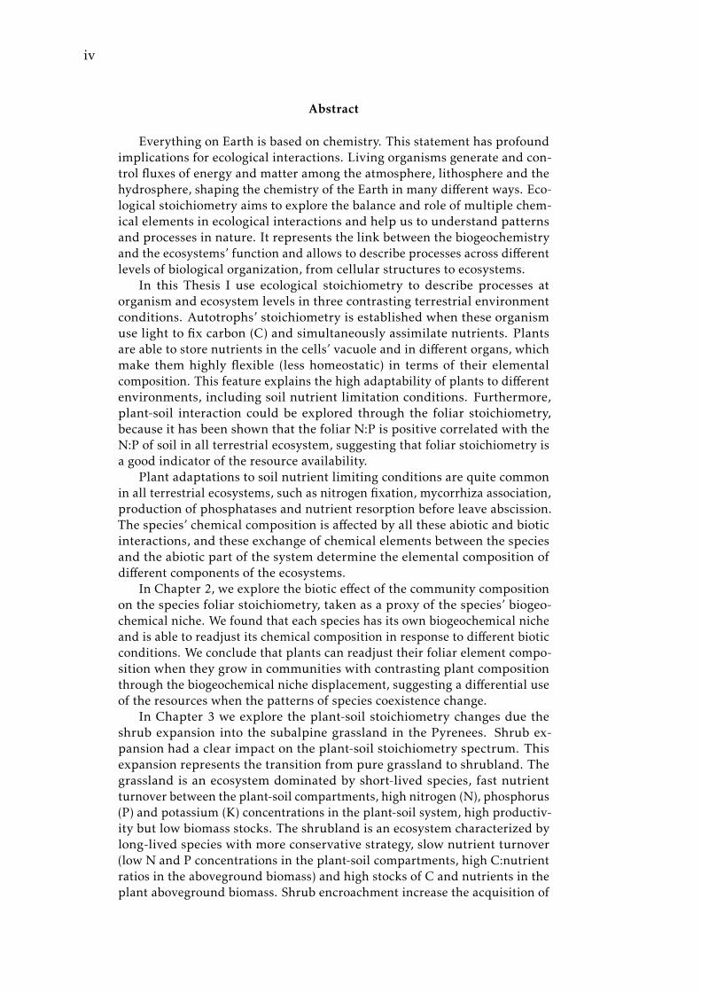
Everything on Earth is based on chemistry. This statement has profoundimplications for ecological interactions. Living organisms generate and con-trol fluxes of energy and matter among the atmosphere, lithosphere and thehydrosphere, shaping the chemistry of the Earth in many different ways. Eco-logical stoichiometry aims to explore the balance and role of multiple chem-ical elements in ecological interactions and help us to understand patternsand processes in nature. It represents the link between the biogeochemistryand the ecosystems’ function and allows to describe processes across differentlevels of biological organization, from cellular structures to ecosystems.
In this Thesis I use ecological stoichiometry to describe processes atorganism and ecosystem levels in three contrasting terrestrial environmentconditions. Autotrophs’ stoichiometry is established when these organismuse light to fix carbon (C) and simultaneously assimilate nutrients. Plantsare able to store nutrients in the cells’ vacuole and in different organs, whichmake them highly flexible (less homeostatic) in terms of their elementalcomposition. This feature explains the high adaptability of plants to differentenvironments, including soil nutrient limitation conditions. Furthermore,plant-soil interaction could be explored through the foliar stoichiometry,because it has been shown that the foliar N:P is positive correlated with theN:P of soil in all terrestrial ecosystem, suggesting that foliar stoichiometry isa good indicator of the resource availability.
Plant adaptations to soil nutrient limiting conditions are quite commonin all terrestrial ecosystems, such as nitrogen fixation, mycorrhiza association,production of phosphatases and nutrient resorption before leave abscission.The species’ chemical composition is affected by all these abiotic and bioticinteractions, and these exchange of chemical elements between the speciesand the abiotic part of the system determine the elemental composition ofdifferent components of the ecosystems.
In Chapter 2, we explore the biotic effect of the community compositionon the species foliar stoichiometry, taken as a proxy of the species’ biogeo-chemical niche. We found that each species has its own biogeochemical nicheand is able to readjust its chemical composition in response to different bioticconditions. We conclude that plants can readjust their foliar element compo-sition when they grow in communities with contrasting plant compositionthrough the biogeochemical niche displacement, suggesting a differential useof the resources when the patterns of species coexistence change.
In Chapter 3 we explore the plant-soil stoichiometry changes due theshrub expansion into the subalpine grassland in the Pyrenees. Shrub ex-pansion had a clear impact on the plant-soil stoichiometry spectrum. Thisexpansion represents the transition from pure grassland to shrubland. Thegrassland is an ecosystem dominated by short-lived species, fast nutrientturnover between the plant-soil compartments, high nitrogen (N), phosphorus(P) and potassium (K) concentrations in the plant-soil system, high productiv-ity but low biomass stocks. The shrubland is an ecosystem characterized bylong-lived species with more conservative strategy, slow nutrient turnover(low N and P concentrations in the plant-soil compartments, high C:nutrientratios in the aboveground biomass) and high stocks of C and nutrients in theplant aboveground biomass. Shrub encroachment increase the acquisition of
v
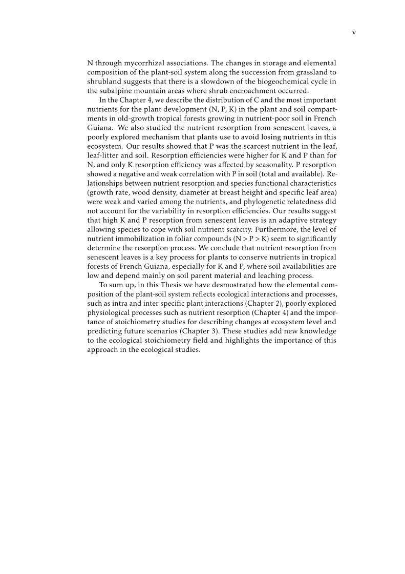
N through mycorrhizal associations. The changes in storage and elementalcomposition of the plant-soil system along the succession from grassland toshrubland suggests that there is a slowdown of the biogeochemical cycle inthe subalpine mountain areas where shrub encroachment occurred.
In the Chapter 4, we describe the distribution of C and the most importantnutrients for the plant development (N, P, K) in the plant and soil compart-ments in old-growth tropical forests growing in nutrient-poor soil in FrenchGuiana. We also studied the nutrient resorption from senescent leaves, apoorly explored mechanism that plants use to avoid losing nutrients in thisecosystem. Our results showed that P was the scarcest nutrient in the leaf,leaf-litter and soil. Resorption efficiencies were higher for K and P than forN, and only K resorption efficiency was affected by seasonality. P resorptionshowed a negative and weak correlation with P in soil (total and available). Re-lationships between nutrient resorption and species functional characteristics(growth rate, wood density, diameter at breast height and specific leaf area)were weak and varied among the nutrients, and phylogenetic relatedness didnot account for the variability in resorption efficiencies. Our results suggestthat high K and P resorption from senescent leaves is an adaptive strategyallowing species to cope with soil nutrient scarcity. Furthermore, the level ofnutrient immobilization in foliar compounds (N > P > K) seem to significantlydetermine the resorption process. We conclude that nutrient resorption fromsenescent leaves is a key process for plants to conserve nutrients in tropicalforests of French Guiana, especially for K and P, where soil availabilities arelow and depend mainly on soil parent material and leaching process.
To sum up, in this Thesis we have desmostrated how the elemental com-position of the plant-soil system reflects ecological interactions and processes,such as intra and inter specific plant interactions (Chapter 2), poorly exploredphysiological processes such as nutrient resorption (Chapter 4) and the impor-tance of stoichiometry studies for describing changes at ecosystem level andpredicting future scenarios (Chapter 3). These studies add new knowledgeto the ecological stoichiometry field and highlights the importance of thisapproach in the ecological studies.
vi
Resumen
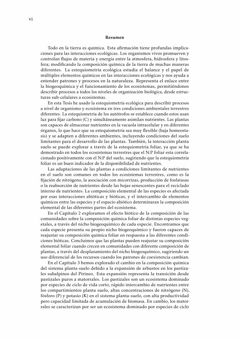
Todo en la tierra es quımica. Esta afirmacion tiene profundas implica-ciones para las interacciones ecologicas. Los organismos vivos promueven ycontrolan flujos de materia y energıa entre la atmosfera, hidrosfera y litos-fera; modificando la composicion quımica de la tierra de muchas manerasdiferentes. La estequiometrıa ecologica estudia el balance y el papel demultiples elementos quımicos en las interacciones ecologicas y nos ayuda aentender patrones y procesos en la naturaleza. Representa el enlace entrela biogeoquımica y el funcionamiento de los ecosistemas, permitiendonosdescribir procesos a todos los niveles de organizacion biologica, desde estruc-turas sub-celulares a ecosistemas.
En esta Tesis he usado la estequiometrıa ecologica para describir procesosa nivel de organismo y ecosistema en tres condiciones ambientales terrestresdiferentes. La estequiometrıa de los autotrofos se establece cuando estos usanluz para fijar carbono (C) y simultaneamente asimilan nutrientes. Las plantasson capaces de almacenar nutrientes en la vacuola intracelular y en diferentesorganos, lo que hace que su estequiometrıa sea muy flexible (baja homeosta-sis) y se adapten a diferentes ambientes, incluyendo condiciones del suelolimitantes para el desarrollo de las plantas. Tambien, la interaccion plantasuelo se puede explorar a traves de la estequiometrıa foliar, ya que se hademostrado en todos los ecosistemas terrestres que el N:P foliar esta correla-cionado positivamente con el N:P del suelo, sugiriendo que la estequiometrıafoliar es un buen indicador de la disponibilidad de nutrientes.
Las adaptaciones de las plantas a condiciones limitantes de nutrientesen el suelo son comunes en todos los ecosistemas terrestres, como es lafijacion de nitrogeno, la asociacion con micorrizas, produccion de fosfatasaso la reabsorcion de nutrientes desde las hojas senescentes para el recicladointerno de nutrientes. La composicion elemental de las especies es afectadapor esas interacciones abioticas y bioticas, y el intercambio de elementosquımicos entre las especies y el espacio abiotico determinaran la composicionelemental de las diferentes partes del ecosistema.
En el Capıtulo 2 exploramos el efecto biotico de la composicion de lascomunidades sobre la composicion quımica foliar de distintas especies veg-etales, a traves del nicho biogeoquımico de cada especie. Encontramos quecada especie presenta su propio nicho biogeoquımico y fueron capaces dereajustar su composicion quımica foliar en respuesta a las diferentes condi-ciones bioticas. Concluimos que las plantas pueden reajustar su composicionelemental foliar cuando crecen en comunidades con diferente composicion deplantas, a traves del desplazamiento del nicho biogeoquımico, sugiriendo unuso diferencial de los recursos cuando los patrones de coexistencia cambian.
En el Capıtulo 3 hemos explorado el cambio en la composicion quımicadel sistema planta-suelo debido a la expansion de arbustos en los pastiza-les subalpinos del Pirineo. Esta expansion representa la transicion desdepastizales puros a matorrales. Los pastizales son un ecosistema dominadopor especies de ciclo de vida corto, rapido intercambio de nutrientes entrelos compartimientos planta suelo, altas concentraciones de nitrogeno (N),fosforo (P) y potasio (K) en el sistema planta-suelo, con alta productividadpero capacidad limitada de acumulacion de biomasa. En cambio, los mator-rales se caracterizan por ser un ecosistema dominado por especies de ciclo
vii
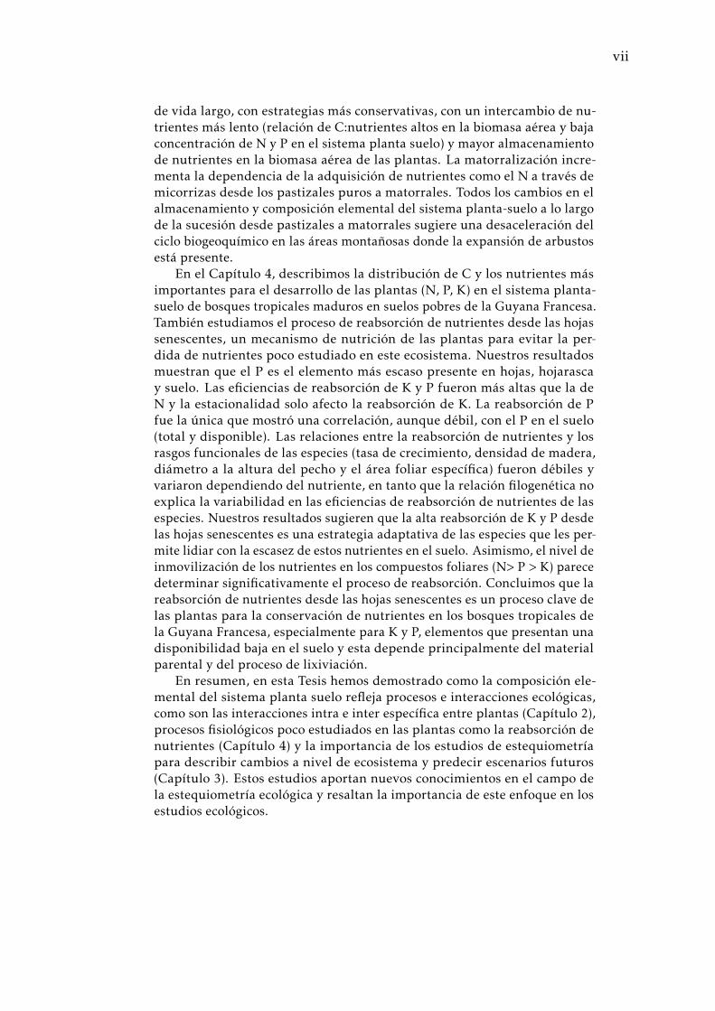
de vida largo, con estrategias mas conservativas, con un intercambio de nu-trientes mas lento (relacion de C:nutrientes altos en la biomasa aerea y bajaconcentracion de N y P en el sistema planta suelo) y mayor almacenamientode nutrientes en la biomasa aerea de las plantas. La matorralizacion incre-menta la dependencia de la adquisicion de nutrientes como el N a traves demicorrizas desde los pastizales puros a matorrales. Todos los cambios en elalmacenamiento y composicion elemental del sistema planta-suelo a lo largode la sucesion desde pastizales a matorrales sugiere una desaceleracion delciclo biogeoquımico en las areas montanosas donde la expansion de arbustosesta presente.
En el Capıtulo 4, describimos la distribucion de C y los nutrientes masimportantes para el desarrollo de las plantas (N, P, K) en el sistema planta-suelo de bosques tropicales maduros en suelos pobres de la Guyana Francesa.Tambien estudiamos el proceso de reabsorcion de nutrientes desde las hojassenescentes, un mecanismo de nutricion de las plantas para evitar la per-dida de nutrientes poco estudiado en este ecosistema. Nuestros resultadosmuestran que el P es el elemento mas escaso presente en hojas, hojarascay suelo. Las eficiencias de reabsorcion de K y P fueron mas altas que la deN y la estacionalidad solo afecto la reabsorcion de K. La reabsorcion de Pfue la unica que mostro una correlacion, aunque debil, con el P en el suelo(total y disponible). Las relaciones entre la reabsorcion de nutrientes y losrasgos funcionales de las especies (tasa de crecimiento, densidad de madera,diametro a la altura del pecho y el area foliar especıfica) fueron debiles yvariaron dependiendo del nutriente, en tanto que la relacion filogenetica noexplica la variabilidad en las eficiencias de reabsorcion de nutrientes de lasespecies. Nuestros resultados sugieren que la alta reabsorcion de K y P desdelas hojas senescentes es una estrategia adaptativa de las especies que les per-mite lidiar con la escasez de estos nutrientes en el suelo. Asimismo, el nivel deinmovilizacion de los nutrientes en los compuestos foliares (N> P > K) parecedeterminar significativamente el proceso de reabsorcion. Concluimos que lareabsorcion de nutrientes desde las hojas senescentes es un proceso clave delas plantas para la conservacion de nutrientes en los bosques tropicales dela Guyana Francesa, especialmente para K y P, elementos que presentan unadisponibilidad baja en el suelo y esta depende principalmente del materialparental y del proceso de lixiviacion.
En resumen, en esta Tesis hemos demostrado como la composicion ele-mental del sistema planta suelo refleja procesos e interacciones ecologicas,como son las interacciones intra e inter especıfica entre plantas (Capıtulo 2),procesos fisiologicos poco estudiados en las plantas como la reabsorcion denutrientes (Capıtulo 4) y la importancia de los estudios de estequiometrıapara describir cambios a nivel de ecosistema y predecir escenarios futuros(Capıtulo 3). Estos estudios aportan nuevos conocimientos en el campo dela estequiometrıa ecologica y resaltan la importancia de este enfoque en losestudios ecologicos.
viii
Article references
• Chapter 2:Urbina, Ifigenia., Sardans, Jordi., Grau, Oriol., Beierkuhnlein, Carl., Jentsch,Anke J., Kreyling, Juergen., & Penuelas, Josep. (2017). Plant communitycomposition affects the species biogeochemical niche. Ecosphere 8(5). doi:e01801. 10.1002/ecs2.1801
• Chapter 3:Urbina, Ifigenia., Grau, Oriol., Sardans, Jordi., Ninot, Josep., & Penuelas,Josep. Encroachment of shrubs into subalpine grasslands in the Pyreneeschanges the plant-soil stoichiometry. Under review in Plant and Soil
• Chapter 4:Urbina, Ifigenia., Grau, Oriol., Sardans, Jordi., Margalef, Olga., Peguero,Guillerom., Ascencio, Dolores., Llusia, Joan., Ogaya, Roma., Gargallo-Garriga,Albert., Va Langenhove, Leandro., Verryckt, Lore T., Courtis, Elodie A., Stahl,Clement., Soong, Jennifer., Chave, Jerome., Herault, Bruno., Janssens, Ivan.,& Penuelas, Josep. High foliar K and P resorption efficiencies in old-growthtropical forests growing on nutrient-poor soils. Manuscript in preparation.
Artwork creditsAll illustrations in the book covers and chapters are by:© Veronica Alvarado Barreto (@nique illustration)
Contents
Contents ix
List of Figures xi
1 Introduction 11.1 Chemestry, life and ecology. A bit of history. . . . . . . . . . . . . . 21.2 Elemental composition of photoautotrophs . . . . . . . . . . . . . . 51.3 The Biogeochemical niche concept, a new approach in the Chemical
Ecology . . . . . . . . . . . . . . . . . . . . . . . . . . . . . . . . . . 61.4 Carbon and nutrients cycles in terrestrial ecosystems . . . . . . . 71.5 Aim of the Thesis . . . . . . . . . . . . . . . . . . . . . . . . . . . . 9
2 Plant community composition affects the species biogeochemical niche 112.1 Introduction . . . . . . . . . . . . . . . . . . . . . . . . . . . . . . . 122.2 Material & Methods . . . . . . . . . . . . . . . . . . . . . . . . . . . 152.3 Results . . . . . . . . . . . . . . . . . . . . . . . . . . . . . . . . . . 172.4 Discussion . . . . . . . . . . . . . . . . . . . . . . . . . . . . . . . . 272.5 Conclusion . . . . . . . . . . . . . . . . . . . . . . . . . . . . . . . . 28
3 Encroachment of shrubs into subalpine grasslands in the Pyrenees changesthe plant-soil stoichiometry 293.1 Introduction . . . . . . . . . . . . . . . . . . . . . . . . . . . . . . . 313.2 Material & Methods . . . . . . . . . . . . . . . . . . . . . . . . . . . 333.3 Results . . . . . . . . . . . . . . . . . . . . . . . . . . . . . . . . . . 383.4 Discussion . . . . . . . . . . . . . . . . . . . . . . . . . . . . . . . . 473.5 Conclusion . . . . . . . . . . . . . . . . . . . . . . . . . . . . . . . . 48
4 High foliar K and P resorption efficiencies in old-growth tropical forestsgrowing on nutrient-poor soils 514.1 Introduction . . . . . . . . . . . . . . . . . . . . . . . . . . . . . . . 524.2 Material & Methods . . . . . . . . . . . . . . . . . . . . . . . . . . . 554.3 Results . . . . . . . . . . . . . . . . . . . . . . . . . . . . . . . . . . 594.4 Discussion . . . . . . . . . . . . . . . . . . . . . . . . . . . . . . . . 664.5 Conclusion . . . . . . . . . . . . . . . . . . . . . . . . . . . . . . . . 70
5 General discussion and conclusions 715.1 Discussion . . . . . . . . . . . . . . . . . . . . . . . . . . . . . . . . 725.2 Conclusions . . . . . . . . . . . . . . . . . . . . . . . . . . . . . . . 77
ix

x CONTENTS
Appendix 2 79
Appendix 3 83
Appendix 4 109
Bibliography 125
List of Figures
1.1 The mineral cycle model. Gersmehl (1976) . . . . . . . . . . . . . 41.2 C, N, P and K cycles in terrestrial ecosystem . . . . . . . . . . . . . 8
2.1 Biogeochemical niche hypothesis . . . . . . . . . . . . . . . . . . . 142.2 PCA monocultures . . . . . . . . . . . . . . . . . . . . . . . . . . . 182.3 PCA heath communities . . . . . . . . . . . . . . . . . . . . . . . . 192.4 Foliar concentrations V. myrtillus . . . . . . . . . . . . . . . . . . . 202.5 Foliar concentrations C. vulgaris . . . . . . . . . . . . . . . . . . . . 212.6 PCA grassland communities . . . . . . . . . . . . . . . . . . . . . . 232.7 PCA A. elatius communities . . . . . . . . . . . . . . . . . . . . . . 252.8 Foliar concentrations H. lanatus . . . . . . . . . . . . . . . . . . . . 262.9 Foliar concentrations A. elatius . . . . . . . . . . . . . . . . . . . . 26
3.1 PCA based on chemical elements (C, N, P, K, Ca, Mg and Fe) in theplant compartment (leaves, leaf-litter) and soil for the successionalstages and vegetation types. . . . . . . . . . . . . . . . . . . . . . . 39
3.2 Stocks of chemical elements (C, N, P, K, Ca, Mg and Fe) in leaves,stems and soil for each successional stage and vegetation type atthe North face . . . . . . . . . . . . . . . . . . . . . . . . . . . . . . 44
3.3 Stocks of chemical elements (C, N, P, K, Ca, Mg and Fe) in leaves,stems and soil for each successional stage and vegetation type atthe South face . . . . . . . . . . . . . . . . . . . . . . . . . . . . . . 46
4.1 Stocks of chemical elements (C, N, P and K) in leaves, leaf-litterand soil in tropical forests . . . . . . . . . . . . . . . . . . . . . . . 61
4.2 N, P and K resorption efficiencies by species . . . . . . . . . . . . . 624.3 N, P and K resorption efficiencies by species both seasons . . . . . 644.4 PCA based on foliar and soil element concentration, nutrient re-
sorption and functional traits in tropical forest . . . . . . . . . . . 65
A.3.1 Study sites Pyrenees . . . . . . . . . . . . . . . . . . . . . . . . . . 84A.3.2 Experimental design Pyrenees . . . . . . . . . . . . . . . . . . . . . 85A.3.3 Correlation between foliar N and δ15N for herbaceous spp and shrubs 86A.3.4 Leaf-litter production per year for each vegetation type in the two
study sites at Pyrenees . . . . . . . . . . . . . . . . . . . . . . . . . 87A.3.5 PCA based on functional traits and foliar elemental composition of
shrub species . . . . . . . . . . . . . . . . . . . . . . . . . . . . . . . 88
xi
A.3.6 PCAs based on the elemental concentrations for leaves, leaf-litter,stems and soil for vegetation types and successional stages at Pyrenees 89
A.4.1 Study sites and experimental design tropical forests . . . . . . . . 110A.4.2 C, N, P and K concentrations in the upper and lower tree canopy
in tropical forests . . . . . . . . . . . . . . . . . . . . . . . . . . . . 111A.4.3 Soil N:P and K:P ratios at the two tropical forests . . . . . . . . . . 112A.4.4 Nutrient resorption efficiencies vs foliar nutrient concentration . . 113A.4.5 P resorption efficiency vs soil P concentration . . . . . . . . . . . . 114A.4.6 N and K resorption efficiencies vs soil N and K concentration . . . 115A.4.7 Nutrient resorption vs functional traits . . . . . . . . . . . . . . . . 116A.4.8 Phylogenetic tree French Guiana . . . . . . . . . . . . . . . . . . . 117
List of Tables
2.1 Characterization of the plant communities EVENT I experiment . 162.2 Anova results element concentration. EVENT I . . . . . . . . . . . 222.3 Anova results element ratios. EVENT I . . . . . . . . . . . . . . . . 24
3.1 GLS results young shrubland vs pure grassland . . . . . . . . . . 413.2 GLS results mature shrubland vs pure grassland . . . . . . . . . . 423.3 GLS results mature shrubland vs young shrubland . . . . . . . . 43
4.1 Stocks of chemical elements (C, N, P and K) in leaves, leaf-litterand soil in tropical forests . . . . . . . . . . . . . . . . . . . . . . . 60
A.2.1 Element concentrations in soil EVENT I experiment . . . . . . . . 80A.2.2 PERMANOVA results by species EVENT I . . . . . . . . . . . . . . 80A.2.3 PERMANOVA results for the species and community EVENT I . . 80A.2.4 Anova results element concentration. Community effect whiting
species . . . . . . . . . . . . . . . . . . . . . . . . . . . . . . . . . . 81A.2.5 Anova results element ratios. Community effect whiting species . 81A.2.6 Tukey HSD Post-hoc comparison Vaccinium myrtillus . . . . . . . . 82A.2.7 Tukey HSD Post-hoc comparison Calluna vulgaris . . . . . . . . . . 82
A.3.1 Ecological characterization of shrubs species in the Pyreenes . . . 90A.3.2 Functional traits of shrubs species (a) . . . . . . . . . . . . . . . . . 91A.3.3 Functional traits of shrubs species (b) . . . . . . . . . . . . . . . . . 92A.3.4 Means for element concentrations and stocks encroachment study 93
A.4.1 Nutrient resorption by species . . . . . . . . . . . . . . . . . . . . . 118A.4.2 Nutrient resorption by species both seasons . . . . . . . . . . . . . 119
xii

List of Tables xiii
A.4.3 Mixed model results for N, P and K resorption efficiencies . . . . . 120A.4.4 Post hoc results for nutrient resorption . . . . . . . . . . . . . . . . 120A.4.5 Mixed model results for N, P and K resorption efficiencies between
seasons . . . . . . . . . . . . . . . . . . . . . . . . . . . . . . . . . . 120A.4.6 N, P and K concentration in leaves a senescent leaves by species . 121A.4.7 C, N, P and K concentrations in soil by plot tropical forest . . . . . 123A.4.8 Phylogenetic signals results . . . . . . . . . . . . . . . . . . . . . . 123

Introduction 1
1
1. Introduction
1.1 Chemestry, life and ecology. A bit of history.
Chemical elements are the essential component of the inert and living matter inthe Earth and their transfer and fluxes among the organisms and their environ-ments are determinant for all ecosystems of the planet. The content and transferfluxes of these chemical elements in organisms and environments constitute anexciting starting point to study the ecology of terrestrial ecosystems. How arechemical elements distributed in the system? What are the biogeochemical feed-backs between the abiotic and biotic parts of the ecosystems, and what are theconsequences of their interactions? What is the chemical composition of livingorganisms?
Eduard Suess, an Austrian geologist, was the first scientist who coined theconcept of biosphere in his book The Origin of the Alps in 1875. He defined thebiosphere as the layer of the Earth where environmental conditions such as tem-perature, water, pressure, chemical compounds and living organisms can be found.Over half a century later, the Russian geochemist Vladimir I Vernadsky expandedthis concept and described the strong relationship between the biosphere and thebiogeochemistry of the Earth in his book The biosphere (Vernadsky 1926). Vernad-sky recognizes that the chemistry of the Earth crust, oceans and the atmosphere ishighly affected by the biosphere. He credits the biosphere as the greatest chemicalforce on earth, and wrote: ‘between the living and inert matter of the biosphere, thereis a single, continuous material and energetic connection, that appears in form of mo-tion of chemical elements to and from living organism depending on the requirementsof life, as feeding, respiration, excretion and reproduction’ (Vernadsky 1938). He alsorefers to the ‘green live organism’ as a fundamental part of the biosphere andpoints to the exchange of gases as the principal evidence of its interaction withthe surrounding environment. Indeed, he anticipated the ecosystem concept andestablish the bases of the ecological biogeochemistry studies. Furthermore, healso highlighted the importance of the human impact on the biogeochemistry ofthe planet describing it as a new planetary phenomenon and coined the concept ofnoosphere as the part of the earth conformed by the humans. He would certainlybe surprised by the extent at which humans have changed the chemistry of ourplanet up to now.
Towards the middle of the last century, biogeochemistry studies mostly fo-cused on the organisms’ chemical composition and the ecosystem functioningbecame more popular. Researchers as G. Evelyn Hutchinson, who wrote the ‘Thebiogeochemistry of the vertebrate excretion’ (Hutchinson 1950) and ‘The Paradoxof Plankton’ (Hutchinson 1961); and Ramon Margalef publications, especiallywith his ‘On Certain Unifying Principles in Ecology’ paper (Margalef 1963) madefundamental contributions to the understanding of the link between the biogeo-chemistry and the structure and stability of ecosystems. Later on, in the 1970s,J. E. Lovelock described in more detail the influence of living organism on thecomposition of the atmosphere (Lovelock 1972). This was previously describedby Vernadsky, but Lovelock’s main contribution was to describe life’s homeostaticcapacity on the planetary environment, which finally gave rise to in the Gaiatheory (Lovelock 1979).
Simultaneously, Philip J. Gersmehl published ‘An alternative biogeography’
2
1.1. Chemestry, life and ecology. A bit of history.
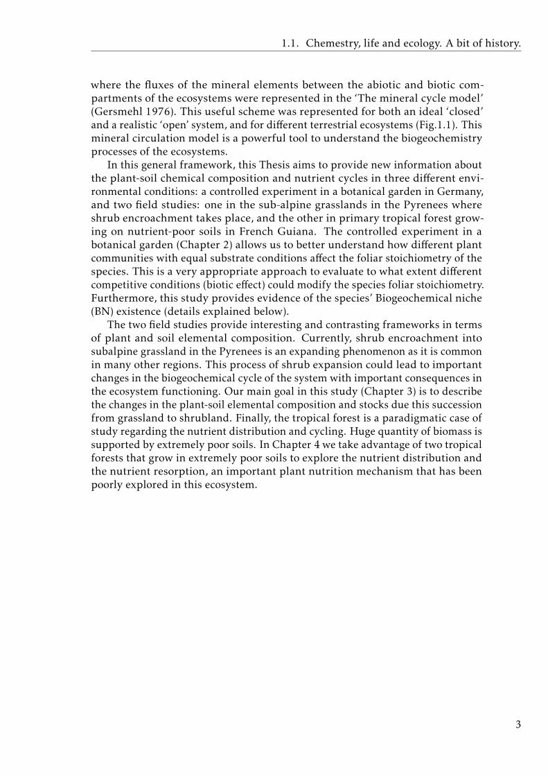
where the fluxes of the mineral elements between the abiotic and biotic com-partments of the ecosystems were represented in the ‘The mineral cycle model’(Gersmehl 1976). This useful scheme was represented for both an ideal ‘closed’and a realistic ‘open’ system, and for different terrestrial ecosystems (Fig.1.1). Thismineral circulation model is a powerful tool to understand the biogeochemistryprocesses of the ecosystems.
In this general framework, this Thesis aims to provide new information aboutthe plant-soil chemical composition and nutrient cycles in three different envi-ronmental conditions: a controlled experiment in a botanical garden in Germany,and two field studies: one in the sub-alpine grasslands in the Pyrenees whereshrub encroachment takes place, and the other in primary tropical forest grow-ing on nutrient-poor soils in French Guiana. The controlled experiment in abotanical garden (Chapter 2) allows us to better understand how different plantcommunities with equal substrate conditions affect the foliar stoichiometry of thespecies. This is a very appropriate approach to evaluate to what extent differentcompetitive conditions (biotic effect) could modify the species foliar stoichiometry.Furthermore, this study provides evidence of the species’ Biogeochemical niche(BN) existence (details explained below).
The two field studies provide interesting and contrasting frameworks in termsof plant and soil elemental composition. Currently, shrub encroachment intosubalpine grassland in the Pyrenees is an expanding phenomenon as it is commonin many other regions. This process of shrub expansion could lead to importantchanges in the biogeochemical cycle of the system with important consequences inthe ecosystem functioning. Our main goal in this study (Chapter 3) is to describethe changes in the plant-soil elemental composition and stocks due this successionfrom grassland to shrubland. Finally, the tropical forest is a paradigmatic case ofstudy regarding the nutrient distribution and cycling. Huge quantity of biomass issupported by extremely poor soils. In Chapter 4 we take advantage of two tropicalforests that grow in extremely poor soils to explore the nutrient distribution andthe nutrient resorption, an important plant nutrition mechanism that has beenpoorly explored in this ecosystem.
3
1. Introduction
Biomass
LitterSoil
dead tissue
decomposition products
uptake by plants
Loss Soil leaching
InputWeathered from rock
Loss litter leaching
Inputdissolved compounds in rainfall
Open systemClose system
Biomass
Litter
Soil
dead tissue
decomposition products
uptake by plants
Shrubland
Tropical ForestMaritime Forest
Tundra
B
L S
B
L S
B
L S
B
L S
(c)
(a) (b)
Figure 1.1: The mineral cycle modeled as three compartments (in circles, B: biomass, L: litterand S: soil) in (a) closed and (b) open system with the basic climatic regulators, temperatureand precipitation (indicated as valves), controlling the rates of nutrient flows. (c) The nutrientcirculation in four idealized terrestrial ecosystem, arrows width indicates the quantity of elementflow expressed as a proportion of the amount stored in the source compartment, and circle sizedenote the amount of nutrient stored in a compartment at steady state. Modified from Gersmehl(1976)
4
1.2. Elemental composition of photoautotrophs
1.2 Elemental composition of photoautotrophs
Carbon (C), Nitrogen (N), Oxygen (O) and Hydrogen (H) are the main elementsthat make life possible. However, living organisms require several other elementsto grow and reproduce successfully, such as phosphorus (P) (essential part ofthe DNA and RNA), potassium (K) (involved in several physiological functions)and in less quantity calcium (Ca), magnesium (Mg) and iron (Fe). C, O and Hare fundamental part of the structure of living organisms, while N, P, K, Ca,Mg are essential nutrients for metabolism and development. Photoautotrophs(autotrophs hereafter) represent the interface between the living and nonlivingsystem in the Earth (Sterner and Elser 2002). Sterner and Elser laid the founda-tions of the ecological stoichiometry studies (from the Greek root: ‘stoicheion’ forelement), which focused on the balance of the multiple chemical elements that arecrucial for ecological interactions and processes. In another definition, ecologicalstoichiometry deals with the patterns and processes associated with the chemicalcontent of the species.
The autotrophs elemental composition is established when they use light tofix carbon (CO2) while simultaneously assimilating inorganic nutrients. Thereare two principal characteristics in the plant cell that mainly determine the plantstoichiometry: the cell wall, rich in C and depleted in P and N; and the presenceof the central vacuole with the capacity to store inorganic and organic nutrientsnot immediately used for growth and reproduction (Sterner and Elser 2002). Also,autotrophs have low homeostasis (the physiological regulation of an organism’sinternal environment) and present nutrient ‘luxury consumption’ which is thenutrient uptake above what is required immediately for growth. Because of this,autotroph organisms exhibit a large variation in their stoichiometric composition(C:N:P, and others), low homeostatic capacity/high stoichiometry flexibility, duethe uncoupling of carbon fixation and nutrient acquisition together with thevariation in the allocation patterns in the different plant organs under differentenvironmental conditions (Sterner and Elser 2002).
The growth rate hypothesis (GRH), developed in aquatic ecosystems (zooplank-ton), proposes that fast-growing organisms will present low biomass C:P andN:P ratios due the higher demand of P allocation to ribosomal RNA necessary tomeet the protein synthesis demands for the faster growth rate (Sterner and Elser2002). However, the applicability of this hypothesis to terrestrial plants is not soclear as it is in planktonic communities. Plants can assign great amounts of Nand P to other functions not directly involved in growth, which makes it difficultto establish a direct relationship between the plant’s C:N:P stoichiometry andgrowth (Penuelas and Sardans 2009; Yu et al. 2012). The plant nutrient ‘luxuryconsumption’ occurs generally when there is another limiting factor as light orother nutrient, and results in an unbalance between the growth and the plant’selemental composition (Sterner and Elser 2002). Moreover, there is an impor-tant intra individual stoichiometry variation especially terrestrial plants, wheredifferent plant compartments (such as leaves, roots, wood and spurs) presentcontrasting elemental compositions.
Despite the difficulty to establish the relationship between autotrophs stoi-chiometry and growth, negative correlation between foliar N:P and maximum
5
1. Introduction
relative growth has been reported for herbaceous and woody species (Gusewell2004). Furthermore, it is well established for a wide range of plants that foliar N:Pis positively correlated with the N:P of the soil, but with great variation withineach climatic area (Sterner and Elser 2002; Sardans et al. 2011; Firn et al. 2019).This evidence suggests that the foliar N:P ratio is a good indicator of the resourceavailability and plant-soil interaction across different ecosystems.
The German botanist Carl Sprengel introduced in the XIX century the first ideaabout ‘law of the minimum’ in the field of agriculture chemistry, which establishesthat plant growth will be constrained by the scarcer nutrient resource rather thanthe total amount available. This idea was expanded by German chemist Justus vonLiebig, and finally popularized as the Liebig’s law of minimum. Nutrient limitingconditions (N, P, K and others) for plant growth are quite common around allterrestrial ecosystems, and plants have adapted to deal with these unfavorableconditions. These adaptations may modify the foliar stoichiometry of the species.
One important strategy present in most terrestrial plants is the fungal my-corrhizas symbiosis association, where fungi provide nutrient to the plant inexchange of C (Bucking et al. 2012a). It has been demonstrated that the exchangeof nutrients (widely described for N) between the fungi and plant induce animportant change in the foliar N isotopic composition of plants. This allows us toestimate the level of ‘mycorrhization’ and the type of mycorrhizas associated toplants and make inferences about N cycling of the systems (Craine et al. 2009a).Another important strategy in terrestrial plants is the symbiosis with nitrogenfixing species in the root’s nodules. This allows plants to fix atmospheric di-nitrogen (N2), making it more independent from the N soil resources and conferscompetitive advantages to life on N-poor soils. This association could imply differ-ent foliar nutrient concentrations and growth between the fixing and non-fixingspecies, having an impact in the N and C cycling of the ecosystem (Battermanet al. 2013b). Furthermore, the production of phosphatases enzymes by plantsrepresents another strategy to deal with scarce nutrient conditions (Vance et al.2003). Phosphatase enzymes release the phosphorus not freely available in soiland make it available for plants in P poor ecosystems, having an important rolein plant growth and ecosystem structure (Hofmann et al. 2016; Batterman etal. 2018). Additionally, the nutrient resorption from senescent leaves beforethe abscission represents an important mechanism that allows plants to be moreindependent from the external conditions and save the metabolic cost of symbioticassociation or enzymes production (Killingbeck 2004; Brant and Chen 2015).
1.3 The Biogeochemical niche concept, a newapproach in the Chemical Ecology
Autotrophs can vary their C:N:P ratios greatly under different available resources.As mentioned above, this is due their capacity to store nutrients, which makesthem highly flexible in their chemical composition. This can result in differentcompetitive strategies among the diverse autotroph species. Plant foliar elementalcomposition has been reported to be linked with species life strategies (Sardans
6
1.4. Carbon and nutrients cycles in terrestrial ecosystems
et al. 2012b; Zechmeister-Boltenstern et al. 2015). Plants with higher growthrates have higher foliar nutrient concentrations (N and P) and lower C:N and C:Pratios than plants with lower growth rates (Agren 2004; Sardans et al. 2012b;Zechmeister-Boltenstern et al. 2015). Moreover, higher N and P concentrationsand lower N:P ratios have been observed in leaves during the growing versus nongrowing seasons, coinciding also with a rise of primary metabolism activity, all ofthem consistent with the GRH expectations (Rivas-Ubach et al. 2012).
The attempt to introduce a new concept which covers all the variables (bioticand abiotic factors) reflected in the species’ chemical composition is not an easytask. The Biogeochemical niche concept (BN) represents a new effort to connect thespecies chemical composition with their evolved genomes and their environmentaland competitive conditions. The BN is defined as the multidimensional space ofthe concentrations of main elements for the organism development (C, N, P, K, Ca,Mg, Fe) in individuals of a given species (Penuelas et al. 2019). The differences inthe biogeochemical niche among species are a function of taxonomy/phylogeneticdistance and of the distinct homeostasis’ capacity. The evolution of the species indifferent stress-disturbance gradients and the genetic variability in their popu-lation would determine the BN flexibility. Thus the species’ BN would also be afunction of the available resources and the capacity of changing would present acontinuum between high homeostasis/low flexibility and low homeostasis/highflexibility (Penuelas et al. 2019). Moreover, the elemental compositions shoulddiffer more among coexisting (sympatric) than among non-coexisting species toavoid competitive pressure (Penuelas et al. 2019). This can explain that species ofthe same genus that recently evolved in different world regions within very dis-tinct communities could have diverged in their elemental composition (Penuelaset al. 2019). As a result, the biogeochemical niche ‘is assumed to be the result ofits taxonomical evolutionary determination and its capacity to respond to changes inexternal conditions’ (Penuelas et al. 2019). The biogeochemical niche is a promis-ing concept that can be used as a proxy of the organism’s performance, whichcomplements the ecological niche theory (Schoener et al. 1986). We will comeback to this concept in Chapter 2 of this Thesis and show how the change in thebiotic conditions are well reflected in the species’ biogeochemical niche.
1.4 Carbon and nutrients cycles in terrestrialecosystems
Plant requirements and nutrient flows will determine the nutrient stocks andavailability in the different ecosystems. In this Thesis we report the changesin plant and soil chemical composition (concentration and stocks) reflectingdifferent plant and ecosystem processes. In Chapter 3 we focus our attentionin the changes at community level in the plant-soil system along the ecologicalsuccession from grassland to shrubland. In contrast, in Chapter 4 we describedthe nutrient distribution (stocks) in the plant-soil system and explore the plantnutrient internal recycling (nutrient resorption) as important plant nutritionmechanisms in tropical forests growing in poor soils. At the ecosystem level, C,
7
1. Introduction
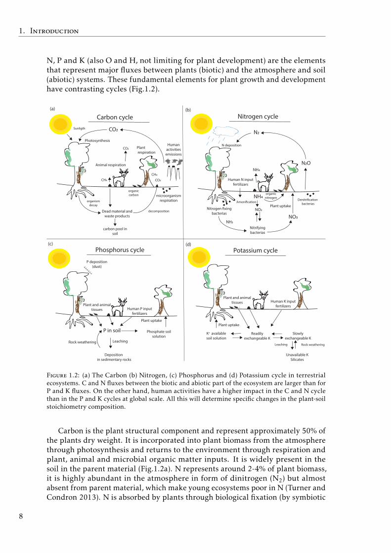
N, P and K (also O and H, not limiting for plant development) are the elementsthat represent major fluxes between plants (biotic) and the atmosphere and soil(abiotic) systems. These fundamental elements for plant growth and developmenthave contrasting cycles (Fig.1.2).
Carbon cycle
CO2
carbon pool in soil
microorganism respiration
Photosynthesis
Sunligth
organic carbon
Dead material and waste products
Plant respiration
Animal respiration
CO2
CO2
CH4CH4
organismdecay
decomposition
Nitrogen cycle
N2
Nitrogen �xing bacterias
Phosphorus cycle
Leaching
P in soil
N deposition
Nitrifying bacterias
Plant uptakeAmoni�cation
NH4
NO2
NO3NH3
Denitri�cation bacterias
N2O
P deposition(dust)
Deposition in sedimentary rocks
Plant and animal tissues
Rock weathering
Phosphate soilsolution
Plant uptake
Potassium cycle
Leaching
Unavailable KSilicates
Plant and animal tissues
Rock weathering
Plant uptake
K+ availablesoil solution
Readily exchangeable K
Slowlyexchangeable K
organic nitrogen
(a) (b)
(c) (d)
Human activities emissions
Human N input fertilizars
Human P input fertilizers
Human K input fertilizers
NH4
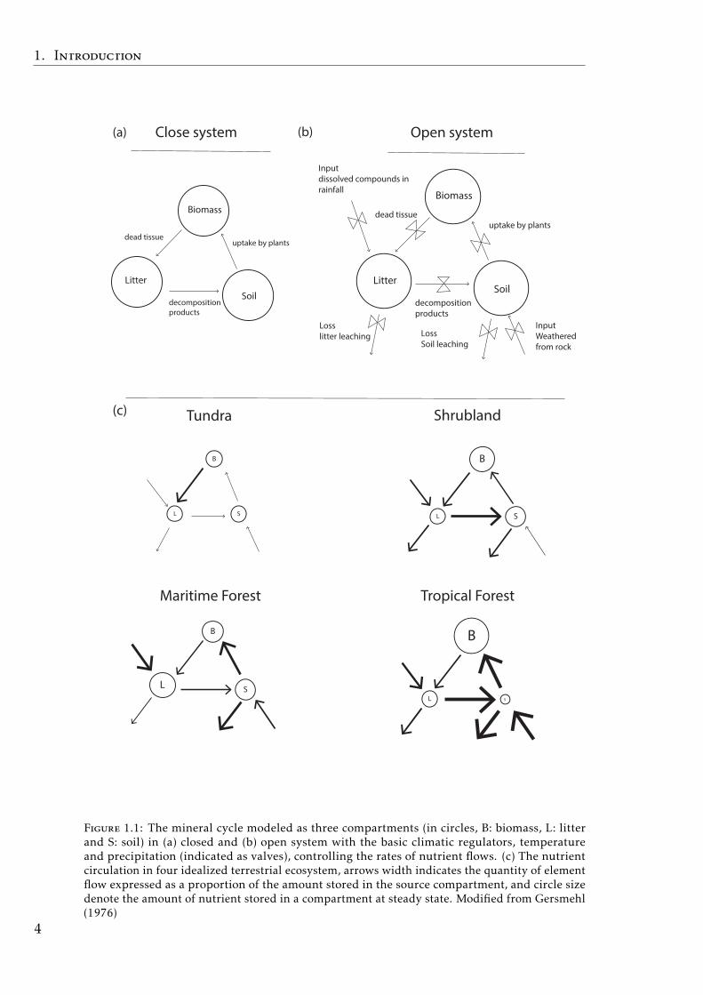
Figure 1.2: (a) The Carbon (b) Nitrogen, (c) Phosphorus and (d) Potassium cycle in terrestrialecosystems. C and N fluxes between the biotic and abiotic part of the ecosystem are larger than forP and K fluxes. On the other hand, human activities have a higher impact in the C and N cyclethan in the P and K cycles at global scale. All this will determine specific changes in the plant-soilstoichiometry composition.
Carbon is the plant structural component and represent approximately 50% ofthe plants dry weight. It is incorporated into plant biomass from the atmospherethrough photosynthesis and returns to the environment through respiration andplant, animal and microbial organic matter inputs. It is widely present in thesoil in the parent material (Fig.1.2a). N represents around 2-4% of plant biomass,it is highly abundant in the atmosphere in form of dinitrogen (N2) but almostabsent from parent material, which make young ecosystems poor in N (Turner andCondron 2013). N is absorbed by plants through biological fixation (by symbiotic
8
1.5. Aim of the Thesis
bacteria association in root nodes), from atmospheric N2 and directly from soil inorganic and inorganic forms via root uptake. It is returned to the system throughplant and animal organic matter which promotes N accumulation and availabilityin soil (Chapin 1980) (Fig.1.2b). In contrast to N, P is highly sequestered in theparent material and is only available for plants by rock weathering (Walker andSyers 1976). Also, atmospheric dust deposition could represent and importantP input in poor soil tropical forests (Gross et al. 2016) (Fig.1.2c). Similarly, Kis mainly present in the parent material in the form of silicates and is providedto plants from by rock weathering and the decomposition of the organic matter(Fig.1.2d). All this implies, more opened cycles for C and N and more closedcycles for P and K between the plant-soil.
As discussed above, all these fluxes (C, N, P, and K) between the biotic andbiotic parts of the ecosystem are reflected in the species stoichiometry. For ex-ample, at global scale N:P ratios in leaves and soil tend to decrease from higherlatitudes towards the tropics, reflecting more N limitation in the cold ecosystemsand more P limitation in the tropical ecosystems. (Sardans et al. 2011). Also,high foliar C:P ratios in the tropical tree are consistent with the P scarcity in theold weathered tropical soils (Sterner and Elser 2002). Patterns in plant and soilC:N:P ratios along successional gradients have predictable consequences on thebiogeochemical cycles and productivity of the system (Sterner and Elser 2002).Furthermore, the availability of nutrients is a main regulator of important pro-cesses and properties from individual to ecosystem level, such as growth (Chapin1980; Elser et al. 2000), primary productivity (Terrer et al. 2017; Vicca et al.2018), forest diversity (John et al. 2007; Hillebrand et al. 2014) and the ecosystemstructure and dynamics (Sayer and Banin 2016; Grau et al. 2017). However, thereare still uncertainties regarding the nutrient role in the ecosystem function andprocesses, especially in a context of climate change, where the chemistry of theEarth has changed drastically during the last years.
1.5 Aim of the Thesis
This Thesis aims to show how the ecological stoichiometry allows us to studyprocesses from the organism to the ecosystem level, through the evaluation of thechemical composition of the plant’s organs and soil in different terrestrial ecosys-tem. This general objective poses novel and challenging questions such as: ‘are theinteractions between plant and soil and the species evolutionary history reflectedin the species Biogeochemical niche?’ and ‘what does the chemical composition ofthe plant-soil system tell us about ecosystem functions and processes?’ that I havetackled in this thesis. The specific questions that I have addressed in the differentchapters are:
• Chapter two: How is the plant community composition reflected in thespecies’ foliar chemical composition? A test of the Biogeochemical niche con-cept.
In this chapter we conducted a controlled experiment to better understand
9

1. Introduction
the biotic effect on the species foliar chemical composition. To do so, we ex-plored the relationships between the plant community composition (numberof species co-habiting in the same plot) on different species’ biogeochemicalniche.
• Chapter three: How is the succession from grassland to shrubland in asub-alpine ecosystem reflected in the plant-soil chemical composition?
In this chapter we explored the stoichiometry changes along the succes-sion from a grassland to a shrubland in the subalpine grassland of theCentral Pyrenees, and how these chemical changes may shape the C andnutrient cycle of this ecosystem.
• Chapter four: How do plants growing in extremely nutrient-poor soils usethe resorption process as a mechanism to deal with nutrient limitation?
In this chapter we explored the cycling of nutrients, the resorption pro-cess, how these processes are controlled, and their importance in old-growthtropical forests growing on nutrient-poor soils.
10
Plant community composition affects thespecies biogeochemical niche 2
11
2. Plant community composition affects the species biogeochemical niche
Abstract
Nutrients are essential for plant development and their availability and stoichio-metric ratios can influence the composition of plant communities. We investigatedthe possibility of the reverse influence: whether the conditions of contrastingspecies coexistence determine foliar element concentrations and plant stoichiom-etry, i.e. species biogeochemical niche (BN). The experiment was conducted atthe Ecological-Botanical Garden of the University of Bayreuth, Germany. Weanalyzed foliar element concentrations of two dwarf shrubs (Calluna vulgaris andVaccinium myrtillus) and two grasses (Holcus lanatus and Arrhenatherum elatius)growing in different community compositions (monocultures and various mixedstands). Foliar nutrient concentrations and stoichiometry (taken as a proxy ofspecies BN) were species-specific; each species showed its own BN in all commu-nities. Furthermore, Vaccinium myrtillus and Holcus lanatus species shifted theirBN in response to changes in their community, accomplishing the ’biogeochemicalniche displacement’ hypothesis. We conclude that plants can readjust their foliarelement concentration if they grow in communities with contrasting plant com-position, suggesting a differential use of element resources when the patterns ofspecies coexistence change. These results also support the complementary nichehypothesis.
• Key words: biogeochemical niche; community composition; grass; home-ostasis; shrub; stoichiometry.
2.1 Introduction
In recent decades plant nutrient stoichiometry, defined as the relative proportionof C and nutrients in plant tissues (leaves, roots, shoots and wood), has gainedsignificant importance in ecological studies (Elser and Urabe 1999, Sterner andElser 2002, Moe et al. 2005, Cross et al. 2005, Elser and Hamilton 2007; Sardans etal. 2012a). It has been found that plant nutrient stoichiometry influences severalecological processes that are pivotal to ecosystem functions and dynamics, suchas plant-herbivore interactions (Daufresne and Loreau 2001, Millett et al. 2005,Newingham et al. 2007), the structure and function of arbuscular mycorrhizae(Johnson 2010) and population dynamics (Andersen et al. 2004). Recent studieshave also found a strong relationship between changes in foliar C:N:K ratios andchanges in foliar metabolites in response to varying environmental conditions(Penuelas and Sardans 2009, Rivas-Ubach et al. 2012). However, the link be-tween foliar nutrient concentration and community composition has proven tobe challenging and remains poorly explored. This is understandable because thecomposition of plant communities depends of several ecological processes andfunctions such as productivity, resource use, nutrient cycling, biotic interactions(Grime 1974, Tilman et al. 1996, Roem 2000), while plant stoichiometry is influ-enced by several factors such as soil fertility, source and quantity of water supply,phylogenetic affiliation and climatic conditions (Sterner and Elser 2002). Addi-tionally, soil layer interactions and competition with microbial communities make
12
2.1. Introduction
it difficult to establish a direct link between soil resources and plant diversity(Hooper and Vitousek 1997), increasing even further the difficulties associatedwith studying the link between plant stoichiometry and community composition.
In this context, (Penuelas et al. 2008, 2019) shed light into the relationshipbetween plant-stoichiometry and plant coexistence. The authors proposed the ’bio-geochemical niche hypothesis’ where species have a species-specific stoichiometryin a multivariate space generated by the contents of macro and micronutrients inplant tissues. This hypothesis is based on coexisting plant species tending to usethe main nutrients N, P and K (and other essential nutrients such as Ca, Mg andS) in differing proportions (Penuelas et al. 2008 and 2010). Since different plantstructures and metabolic processes have distinct and divergent requirements foreach of the essential nutrients, the species-specific biogeochemical niches shouldbe the result of species specialization to particular abiotic and biotic conditions.BN should reflect the different species-specific strategies of growth and uptake ofresources and the differences in soil space and time occupation reducing directcompetition among sympatric species and optimizing the nutrient use by theoverall community. BN also hypothesized that the existence if stoichiometricflexibility (the capacity to change the biogeochemical niche) of a species is animportant trait, as it is related to the quality of plants tissues and their capacityto cope with changes in environmental conditions. Building further on this hy-pothesis, Yu et al. (2010) argued that species exhibit stoichiometric flexibility inresponse to environmental changes (including ontogenic and seasonal changes)and competitive situations, probably under a tradeoff between the stoichiometryflexibility and homeostatic regulation (the maintenance of constant internal con-ditions in the face of externally imposed variation). Recent studies in Spanish andEuropean forests have shown that elemental stoichiometries of different forestspecies were strongly determined genetically which is consistent with their long-term adaptation to specific abiotic and biotic environments leading to optimizedmetabolic and physiological functions and morphological structures determiningthe specific use of various nutrients (Sardans et al. 2015, 2016). These studieshave also shown that current climate is also an important driver of uptake andnutrient use and that BN should reflect trade-offs among several functions suchas plant growth, resource storage and/or anti-stress mechanisms for maximizingplant fitness in each of particular climate. More differences in foliar compositionstoichiometry among sympatric species than among allopatric species have beenreported (Sardans et al. 2015, 2016). The BN hypothesis thus claim that allspecies are adapted, to some extent, to different combinations of environmentalfactors implying a trade-off between different basic functions such as growth rates,reproduction and stress tolerance. The different BN can also be taken as a finalresult of an optimum adaptation to environmental gradients and can be comparedto the proposed ecological strategies as for example the Grime R-C-S model (1977)where different species can be placed in a specific ’space’ in the gradient amongthese different ecological strategies.
Following Penuelas et al. (2008, 2019) BN hypothesis, we here investigatedthe inverse relationship between the changes in species coexistence and the BN ofspecies. We aimed to determine if the composition of plant communities affects theBN of individual species. We included as many elements as possible in the analysis
13
2. Plant community composition affects the species biogeochemical niche
because of the well known importance of several elements like K, Mg, S and Ca inplant physiology in water stress avoiding strategies, photosynthetic machinery,regulation of ion balance (homeostasis) in chloroplast and vacuoles, transport ofsugar into the phloem and secondary metabolism (Sawhney Zelitch 1969; Knightet al. 1991; Romeis et al. 2001; Shaul 2002; Cakmak 2005; Franceschi Nakata2005; Rennenberg et al. 2007; Gill Tuteja 2011; Sardans Penuelas 2015). Ourmain research question was: Are plants able to modify their foliar stoichiometry(species BN) in response to varying species coexistence?
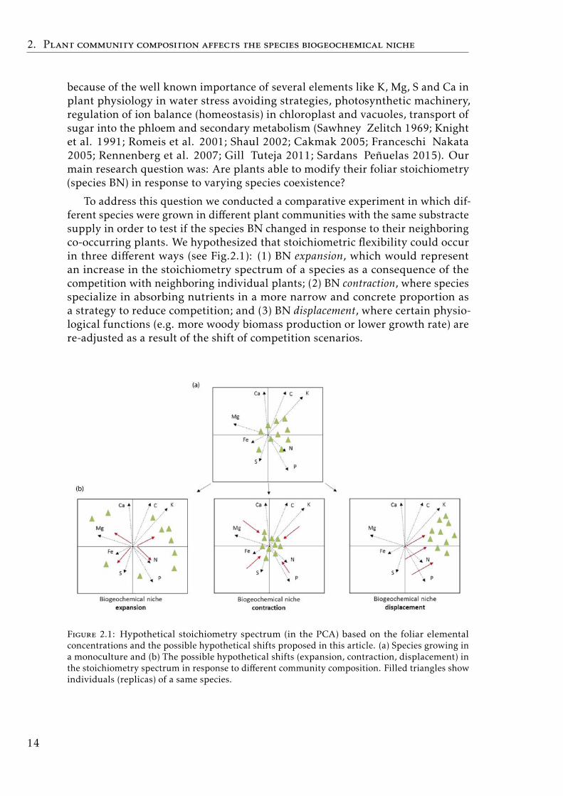
To address this question we conducted a comparative experiment in which dif-ferent species were grown in different plant communities with the same substractesupply in order to test if the species BN changed in response to their neighboringco-occurring plants. We hypothesized that stoichiometric flexibility could occurin three different ways (see Fig.2.1): (1) BN expansion, which would representan increase in the stoichiometry spectrum of a species as a consequence of thecompetition with neighboring individual plants; (2) BN contraction, where speciesspecialize in absorbing nutrients in a more narrow and concrete proportion asa strategy to reduce competition; and (3) BN displacement, where certain physio-logical functions (e.g. more woody biomass production or lower growth rate) arere-adjusted as a result of the shift of competition scenarios.
Figure 2.1: Hypothetical stoichiometry spectrum (in the PCA) based on the foliar elementalconcentrations and the possible hypothetical shifts proposed in this article. (a) Species growing ina monoculture and (b) The possible hypothetical shifts (expansion, contraction, displacement) inthe stoichiometry spectrum in response to different community composition. Filled triangles showindividuals (replicas) of a same species.
14
2.2. Material & Methods
2.2 Material & Methods
Experimental setup
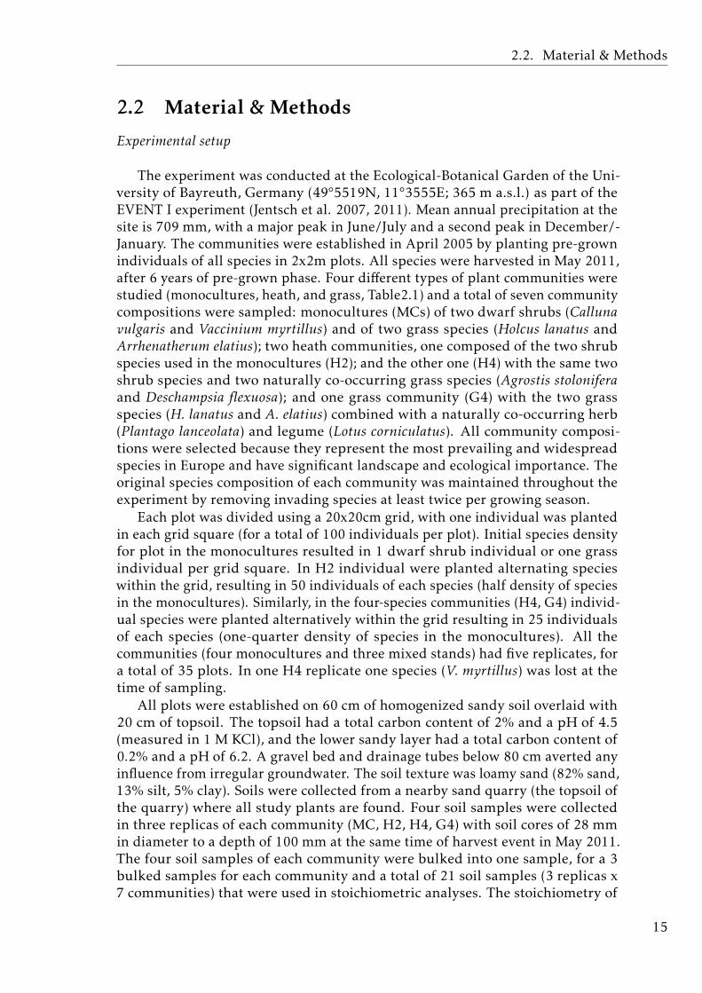
The experiment was conducted at the Ecological-Botanical Garden of the Uni-versity of Bayreuth, Germany (49°5519N, 11°3555E; 365 m a.s.l.) as part of theEVENT I experiment (Jentsch et al. 2007, 2011). Mean annual precipitation at thesite is 709 mm, with a major peak in June/July and a second peak in December/-January. The communities were established in April 2005 by planting pre-grownindividuals of all species in 2x2m plots. All species were harvested in May 2011,after 6 years of pre-grown phase. Four different types of plant communities werestudied (monocultures, heath, and grass, Table2.1) and a total of seven communitycompositions were sampled: monocultures (MCs) of two dwarf shrubs (Callunavulgaris and Vaccinium myrtillus) and of two grass species (Holcus lanatus andArrhenatherum elatius); two heath communities, one composed of the two shrubspecies used in the monocultures (H2); and the other one (H4) with the same twoshrub species and two naturally co-occurring grass species (Agrostis stoloniferaand Deschampsia flexuosa); and one grass community (G4) with the two grassspecies (H. lanatus and A. elatius) combined with a naturally co-occurring herb(Plantago lanceolata) and legume (Lotus corniculatus). All community composi-tions were selected because they represent the most prevailing and widespreadspecies in Europe and have significant landscape and ecological importance. Theoriginal species composition of each community was maintained throughout theexperiment by removing invading species at least twice per growing season.
Each plot was divided using a 20x20cm grid, with one individual was plantedin each grid square (for a total of 100 individuals per plot). Initial species densityfor plot in the monocultures resulted in 1 dwarf shrub individual or one grassindividual per grid square. In H2 individual were planted alternating specieswithin the grid, resulting in 50 individuals of each species (half density of speciesin the monocultures). Similarly, in the four-species communities (H4, G4) individ-ual species were planted alternatively within the grid resulting in 25 individualsof each species (one-quarter density of species in the monocultures). All thecommunities (four monocultures and three mixed stands) had five replicates, fora total of 35 plots. In one H4 replicate one species (V. myrtillus) was lost at thetime of sampling.
All plots were established on 60 cm of homogenized sandy soil overlaid with20 cm of topsoil. The topsoil had a total carbon content of 2% and a pH of 4.5(measured in 1 M KCl), and the lower sandy layer had a total carbon content of0.2% and a pH of 6.2. A gravel bed and drainage tubes below 80 cm averted anyinfluence from irregular groundwater. The soil texture was loamy sand (82% sand,13% silt, 5% clay). Soils were collected from a nearby sand quarry (the topsoil ofthe quarry) where all study plants are found. Four soil samples were collectedin three replicas of each community (MC, H2, H4, G4) with soil cores of 28 mmin diameter to a depth of 100 mm at the same time of harvest event in May 2011.The four soil samples of each community were bulked into one sample, for a 3bulked samples for each community and a total of 21 soil samples (3 replicas x7 communities) that were used in stoichiometric analyses. The stoichiometry of
15
2. Plant community composition affects the species biogeochemical niche
Table 2.1: Characterization of the plant communities of the EVENT I experiment.
Community Description Species
MC Monocultures of four targetspecies
Calluna vulgaris, Vaccinium myr-tillus, Holcus lanatus, Arrhen-atherum elatius
H2 Two species, one functionalgroup (dwarfshrub)
Calluna vulgaris and Vacciniummyrtillus
H4 Four species, two functionalgroups (dwarf shrubs andgrass)
Calluna vulgaris, Vacciniummyrtillus, Agrostis stolonifera,Deschampsia flexuosa
G4 Four species, three func-tional groups (grass, herb andlegum)
Holcus lanatus, Arrhenatherumelatius, Plantago lanceolata, Lotuscorniculatus
the soil nutrients did not differ significantly among the communities; the totalelement concentrations are presented in the supporting information section (TableA.2.1).
Sampling, chemical analysis and biomass calculation
All species were harvested in May 2011 for chemical analyses. An equal num-ber of top and bottom leaves were collected from mature, reproductive individuals.We collected a total of 15 foliar samples from each species of dwarf shrub and atotal of 10 foliar samples from each grass species. Sampling was conducted in twodiffering ways depending on the occurrence or not of regeneration within the plots.When no regeneration occurred (true for the both dwarf shrubs Calluna vulgarisand Vaccinium myrtillus) 20x40 cm sampling frames were centered in two dwarfshrubs for H2 and H4, and a 20x20 sampling frame centered in each shrub for themonocultures. When regeneration occurred (G4 and grasses monocultures) the20x40 sampling frames were placed randomly in every community compositionbecause it was not possible to locate originally planted individuals. The biomassper area was calculated in 20x40cm (0.08m2) of sampling area. In the dwarfshrubs monoculture, because the sampling was carried out with 20x20 frame, thevalue was corrected by multiplying by two, resulting in the same area.
The collected leaves were oven-dried at 70 °C for 72 h, pulverized, re-driedat 70 °C for 48 h and stored in desiccators until analyzed (<15 days). C and Nconcentrations were determined for 0.7-0.9 mg of pulverized dried samples bycombustion coupled to gas chromatography with an Elemental Analyzer CHNSEurovector 3011 Thermo Electron Gas Chromatograph, model NA 2100 (CEInstruments/Thermo Electron, Milan, Italy). The concentrations of the otherelements (P, K, Ca, Mg, S and Fe) were determined for 0.25 g of pulverized driedsample dissolved with an acidic mixture of HNO3 (60% w/v) and H2O2 (30% w/v)and digested in a MARSXpress microwave system (CEM GmbH, Kamp-Lintfort,Germany). The digests were then diluted to a final volume of 50 mL with ultrapurewater and 1% HNO3. Blank solutions (5 mL of HNO3 and 2 mL of H2O2 with
16
2.3. Results
no sample) were regularly analyzed. The concentrations of Ca, K, Mg, S, P andFe after digestion were analyzed by ICP-OES inductively coupled plasma opticalemission spectrometry (Optima 4300 DV, Perkin-Elmer, Waltham, USA). Theaccuracy of the biomass digestions and analytical procedures were assessed witha certified biomass NIST 1573a (tomato leaf, NIST, Gaitherburg, USA) standards.
Statistical analysis
Principal component analyses (PCAs) were conducted based on the foliarstoichiometric data of each species in order to explore the possible different groupsformed by the community factor. A complementary PERMANOVA analysis wasconducted to test the statistical significance of the groups. One-way ANOVAswere conducted using element concentrations and C:N, C:P, C:K, N:P, N:K andP:K ratios as dependent variables and community as a categorical factor for eachspecies in order to evaluate the differences in elements concentrations within thedifferent communities. ANOVA was also applied to test differences in speciesbiomass per area in the different communities. We used Tukey’s HSD test and thepairwise test with Bonferroni corrections to differentiate community groups. Priorto the statistical analyses, we tested for normality and homogeneity of variances ofelement concentrations using the Shapiro-Wilk normality test. Also, the residualsversus the expected plots and the normal qq-plots of the linear models wereexamined. All statistical analyses were conducted with R packages in R 3.2.1(RCoreTeam 2017). FactoMineR package (Le et al. 2008) was used for the PCAanalysis, Vegan package (Oksanen et al. 2017) for the ANOVAs, Permute packagefor the PERMANOVA analysis and ggplot2 for graphics (Wickham 2009).
2.3 Results
Monoculture communities
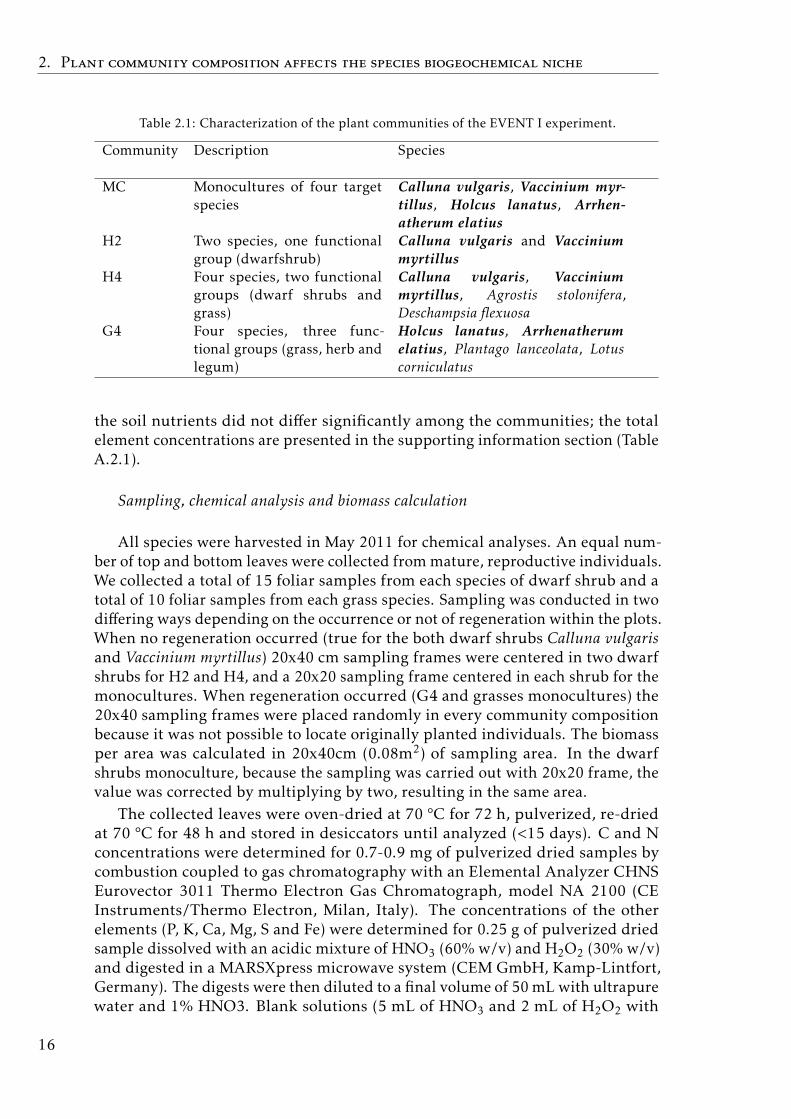
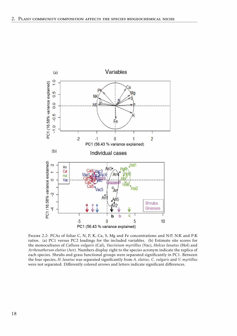
The PCA of the four monocultures showed the separation of the dwarf-shruband grass functional groups on the first axis (p< 0.0001), which explained 56.4%of the variability (Fig.2.2). Furthermore, the grass species were separated alongthe PC1 axis (p< 0.0001), while the shrubs were not separated.
Heath communities (H2 vs H4 vs MCs)
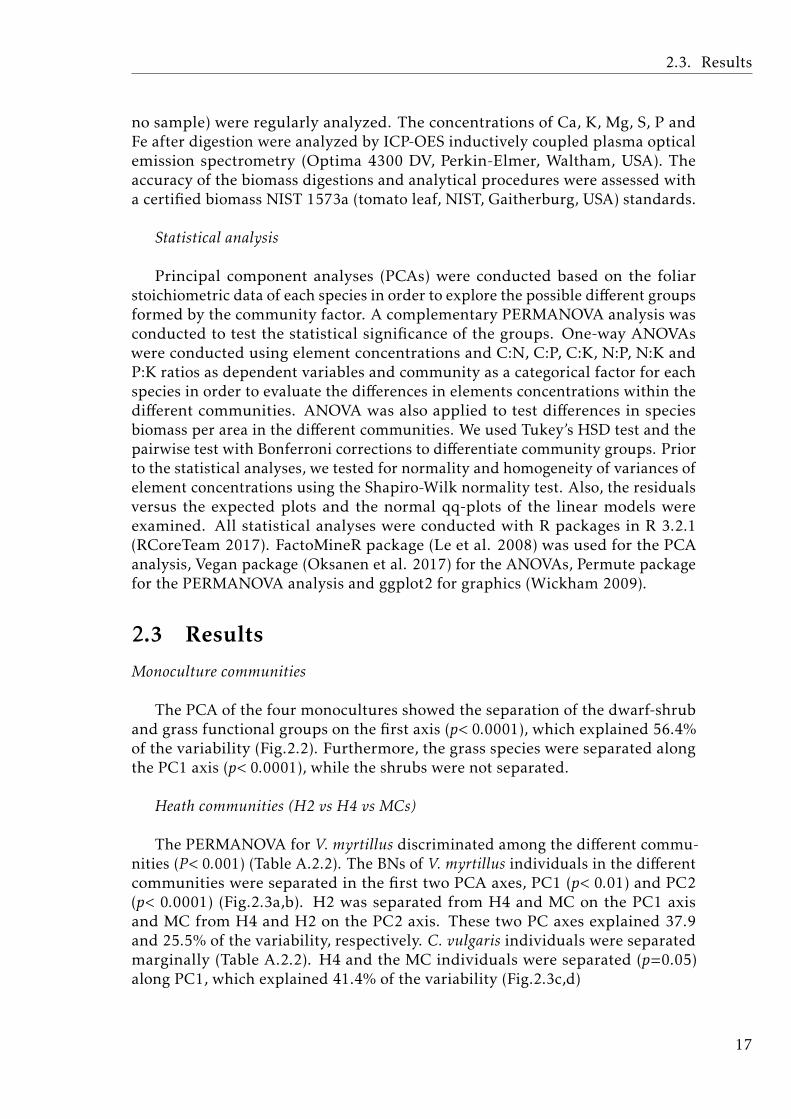
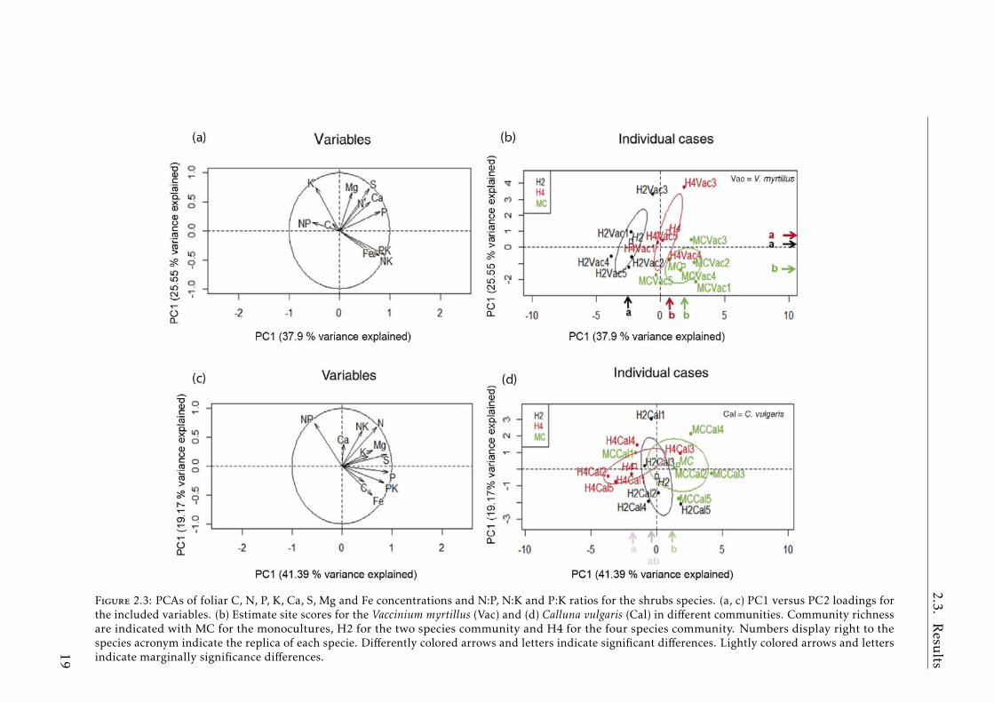
The PERMANOVA for V. myrtillus discriminated among the different commu-nities (P< 0.001) (Table A.2.2). The BNs of V. myrtillus individuals in the differentcommunities were separated in the first two PCA axes, PC1 (p< 0.01) and PC2(p< 0.0001) (Fig.2.3a,b). H2 was separated from H4 and MC on the PC1 axisand MC from H4 and H2 on the PC2 axis. These two PC axes explained 37.9and 25.5% of the variability, respectively. C. vulgaris individuals were separatedmarginally (Table A.2.2). H4 and the MC individuals were separated (p=0.05)along PC1, which explained 41.4% of the variability (Fig.2.3c,d)
17
2. Plant community composition affects the species biogeochemical niche
Figure 2.2: PCAs of foliar C, N, P, K, Ca, S, Mg and Fe concentrations and N:P, N:K and P:Kratios. (a) PC1 versus PC2 loadings for the included variables. (b) Estimate site scores forthe monocultures of Calluna vulgaris (Cal), Vaccinium myrtillus (Vac), Holcus lanatus (Hol) andArrhenatherum elatius (Arr). Numbers display right to the species acronym indicate the replica ofeach species. Shrubs and grass functional groups were separated significantly in PC1. Betweenthe four species, H. lanatus was separated significantly from A. elatius. C. vulgaris and V. myrtilluswere not separated. Differently colored arrows and letters indicate significant differences.
18
2.3.R
esults
Figure 2.3: PCAs of foliar C, N, P, K, Ca, S, Mg and Fe concentrations and N:P, N:K and P:K ratios for the shrubs species. (a, c) PC1 versus PC2 loadings forthe included variables. (b) Estimate site scores for the Vaccinium myrtillus (Vac) and (d) Calluna vulgaris (Cal) in different communities. Community richnessare indicated with MC for the monocultures, H2 for the two species community and H4 for the four species community. Numbers display right to thespecies acronym indicate the replica of each specie. Differently colored arrows and letters indicate significant differences. Lightly colored arrows and lettersindicate marginally significance differences.
19
2. Plant community composition affects the species biogeochemical niche
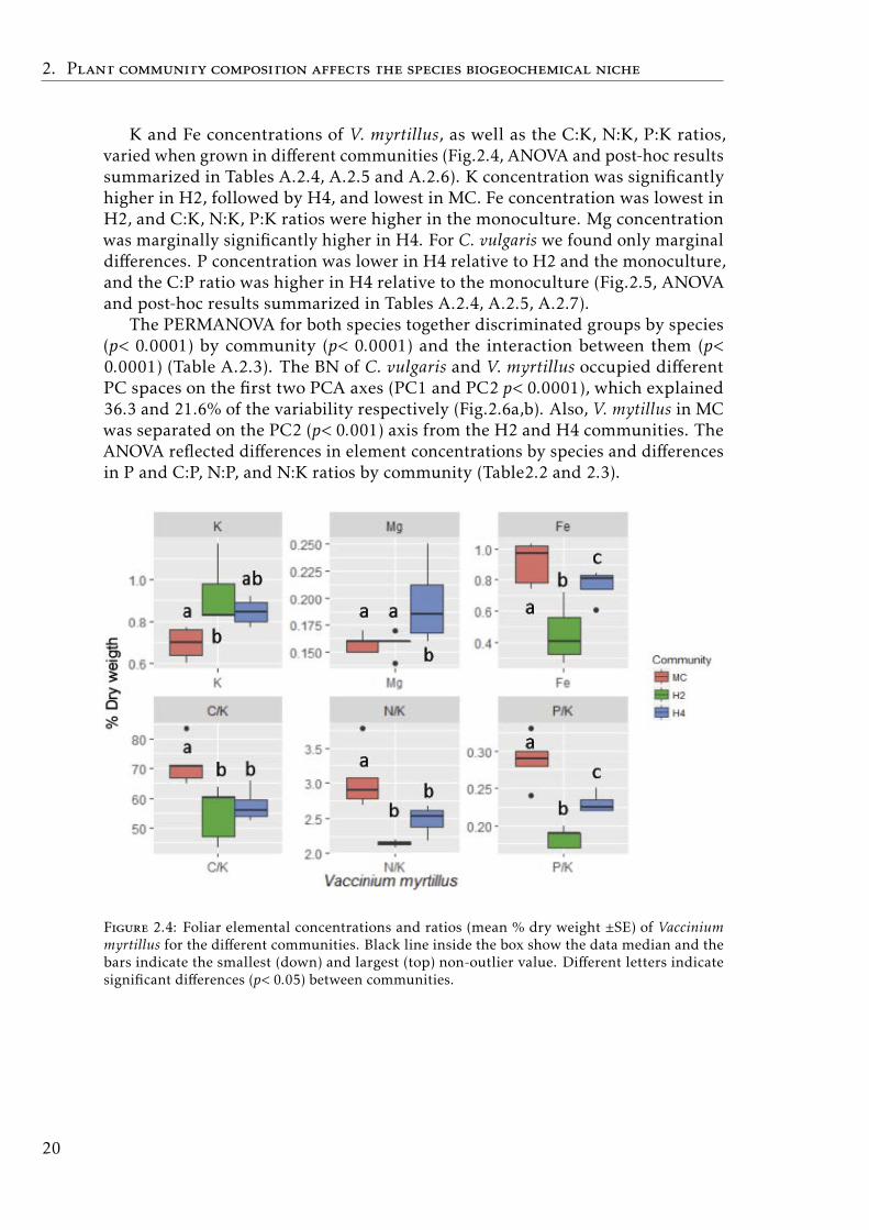
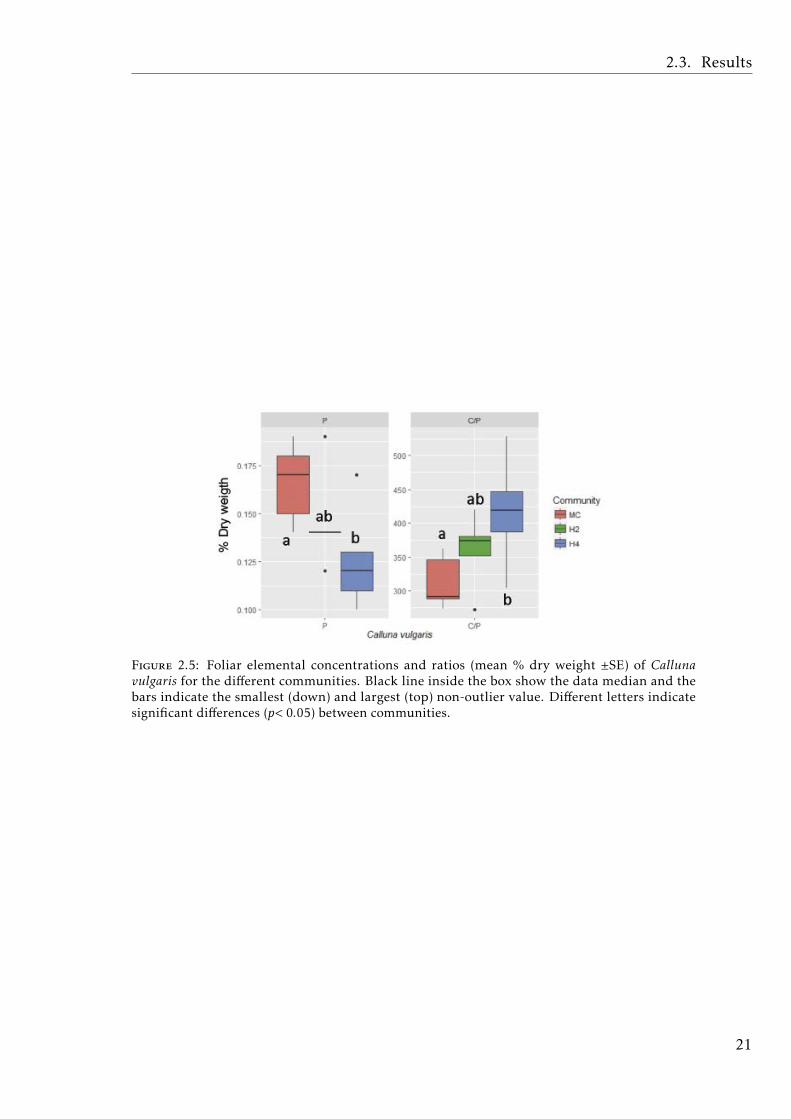
K and Fe concentrations of V. myrtillus, as well as the C:K, N:K, P:K ratios,varied when grown in different communities (Fig.2.4, ANOVA and post-hoc resultssummarized in Tables A.2.4, A.2.5 and A.2.6). K concentration was significantlyhigher in H2, followed by H4, and lowest in MC. Fe concentration was lowest inH2, and C:K, N:K, P:K ratios were higher in the monoculture. Mg concentrationwas marginally significantly higher in H4. For C. vulgaris we found only marginaldifferences. P concentration was lower in H4 relative to H2 and the monoculture,and the C:P ratio was higher in H4 relative to the monoculture (Fig.2.5, ANOVAand post-hoc results summarized in Tables A.2.4, A.2.5, A.2.7).
The PERMANOVA for both species together discriminated groups by species(p< 0.0001) by community (p< 0.0001) and the interaction between them (p<0.0001) (Table A.2.3). The BN of C. vulgaris and V. myrtillus occupied differentPC spaces on the first two PCA axes (PC1 and PC2 p< 0.0001), which explained36.3 and 21.6% of the variability respectively (Fig.2.6a,b). Also, V. mytillus in MCwas separated on the PC2 (p< 0.001) axis from the H2 and H4 communities. TheANOVA reflected differences in element concentrations by species and differencesin P and C:P, N:P, and N:K ratios by community (Table2.2 and 2.3).
Figure 2.4: Foliar elemental concentrations and ratios (mean % dry weight ±SE) of Vacciniummyrtillus for the different communities. Black line inside the box show the data median and thebars indicate the smallest (down) and largest (top) non-outlier value. Different letters indicatesignificant differences (p< 0.05) between communities.
20
2.3. Results
Figure 2.5: Foliar elemental concentrations and ratios (mean % dry weight ±SE) of Callunavulgaris for the different communities. Black line inside the box show the data median and thebars indicate the smallest (down) and largest (top) non-outlier value. Different letters indicatesignificant differences (p< 0.05) between communities.
21
2.Plantcommunitycompositionaffectsthespeciesbiogeochemicalniche
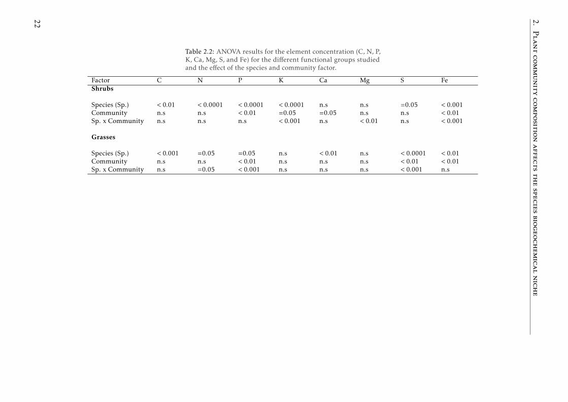
Table 2.2: ANOVA results for the element concentration (C, N, P,K, Ca, Mg, S, and Fe) for the different functional groups studiedand the effect of the species and community factor.
Factor C N P K Ca Mg S FeShrubs
Species (Sp.) < 0.01 < 0.0001 < 0.0001 < 0.0001 n.s n.s =0.05 < 0.001Community n.s n.s < 0.01 =0.05 =0.05 n.s n.s < 0.01Sp. x Community n.s n.s n.s < 0.001 n.s < 0.01 n.s < 0.001
Grasses
Species (Sp.) < 0.001 =0.05 =0.05 n.s < 0.01 n.s < 0.0001 < 0.01Community n.s n.s < 0.01 n.s n.s n.s < 0.01 < 0.01Sp. x Community n.s =0.05 < 0.001 n.s n.s n.s < 0.001 n.s
22
2.3.R
esults
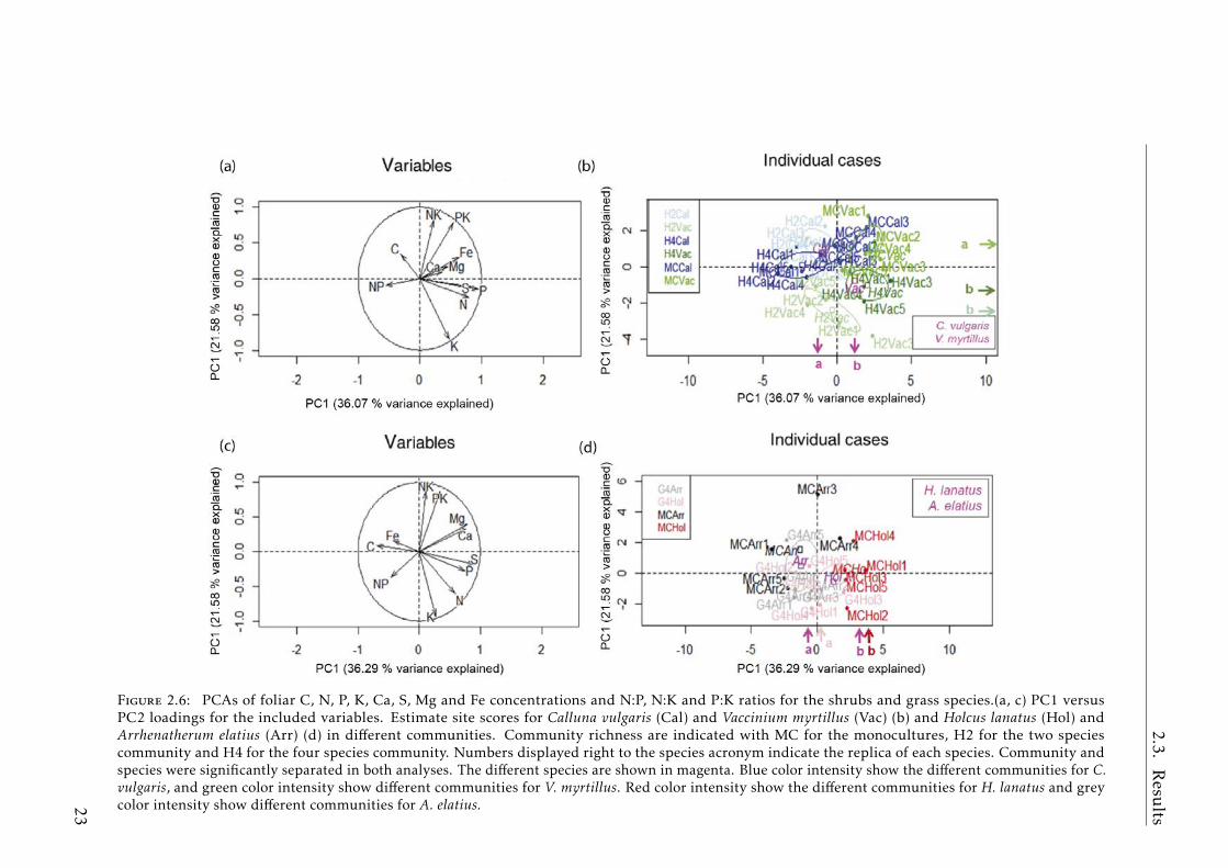
Figure 2.6: PCAs of foliar C, N, P, K, Ca, S, Mg and Fe concentrations and N:P, N:K and P:K ratios for the shrubs and grass species.(a, c) PC1 versusPC2 loadings for the included variables. Estimate site scores for Calluna vulgaris (Cal) and Vaccinium myrtillus (Vac) (b) and Holcus lanatus (Hol) andArrhenatherum elatius (Arr) (d) in different communities. Community richness are indicated with MC for the monocultures, H2 for the two speciescommunity and H4 for the four species community. Numbers displayed right to the species acronym indicate the replica of each species. Community andspecies were significantly separated in both analyses. The different species are shown in magenta. Blue color intensity show the different communities for C.vulgaris, and green color intensity show different communities for V. myrtillus. Red color intensity show the different communities for H. lanatus and greycolor intensity show different communities for A. elatius.23
2. Plant community composition affects the species biogeochemical niche
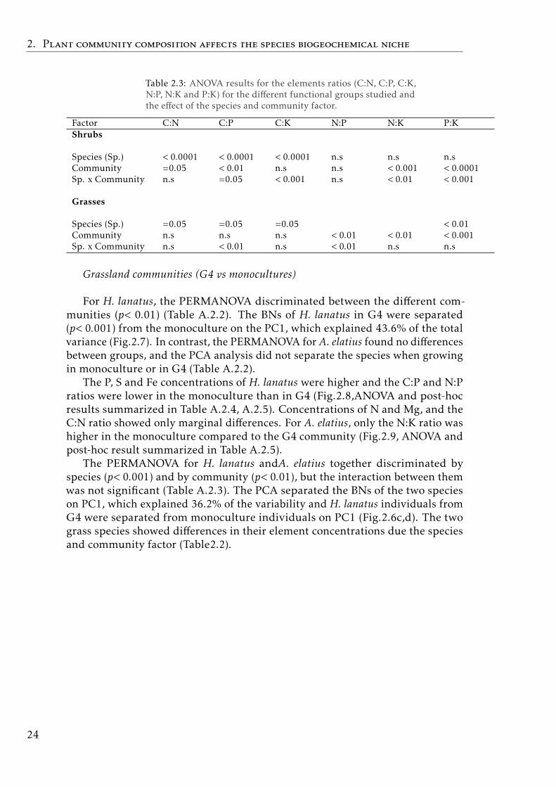
Table 2.3: ANOVA results for the elements ratios (C:N, C:P, C:K,N:P, N:K and P:K) for the different functional groups studied andthe effect of the species and community factor.
Factor C:N C:P C:K N:P N:K P:KShrubs
Species (Sp.) < 0.0001 < 0.0001 < 0.0001 n.s n.s n.sCommunity =0.05 < 0.01 n.s n.s < 0.001 < 0.0001Sp. x Community n.s =0.05 < 0.001 n.s < 0.01 < 0.001
Grasses
Species (Sp.) =0.05 =0.05 =0.05 < 0.01Community n.s n.s n.s < 0.01 < 0.01 < 0.001Sp. x Community n.s < 0.01 n.s < 0.01 n.s n.s
Grassland communities (G4 vs monocultures)
For H. lanatus, the PERMANOVA discriminated between the different com-munities (p< 0.01) (Table A.2.2). The BNs of H. lanatus in G4 were separated(p< 0.001) from the monoculture on the PC1, which explained 43.6% of the totalvariance (Fig.2.7). In contrast, the PERMANOVA for A. elatius found no differencesbetween groups, and the PCA analysis did not separate the species when growingin monoculture or in G4 (Table A.2.2).
The P, S and Fe concentrations of H. lanatus were higher and the C:P and N:Pratios were lower in the monoculture than in G4 (Fig.2.8,ANOVA and post-hocresults summarized in Table A.2.4, A.2.5). Concentrations of N and Mg, and theC:N ratio showed only marginal differences. For A. elatius, only the N:K ratio washigher in the monoculture compared to the G4 community (Fig.2.9, ANOVA andpost-hoc result summarized in Table A.2.5).
The PERMANOVA for H. lanatus andA. elatius together discriminated byspecies (p< 0.001) and by community (p< 0.01), but the interaction between themwas not significant (Table A.2.3). The PCA separated the BNs of the two specieson PC1, which explained 36.2% of the variability and H. lanatus individuals fromG4 were separated from monoculture individuals on PC1 (Fig.2.6c,d). The twograss species showed differences in their element concentrations due the speciesand community factor (Table2.2).
24
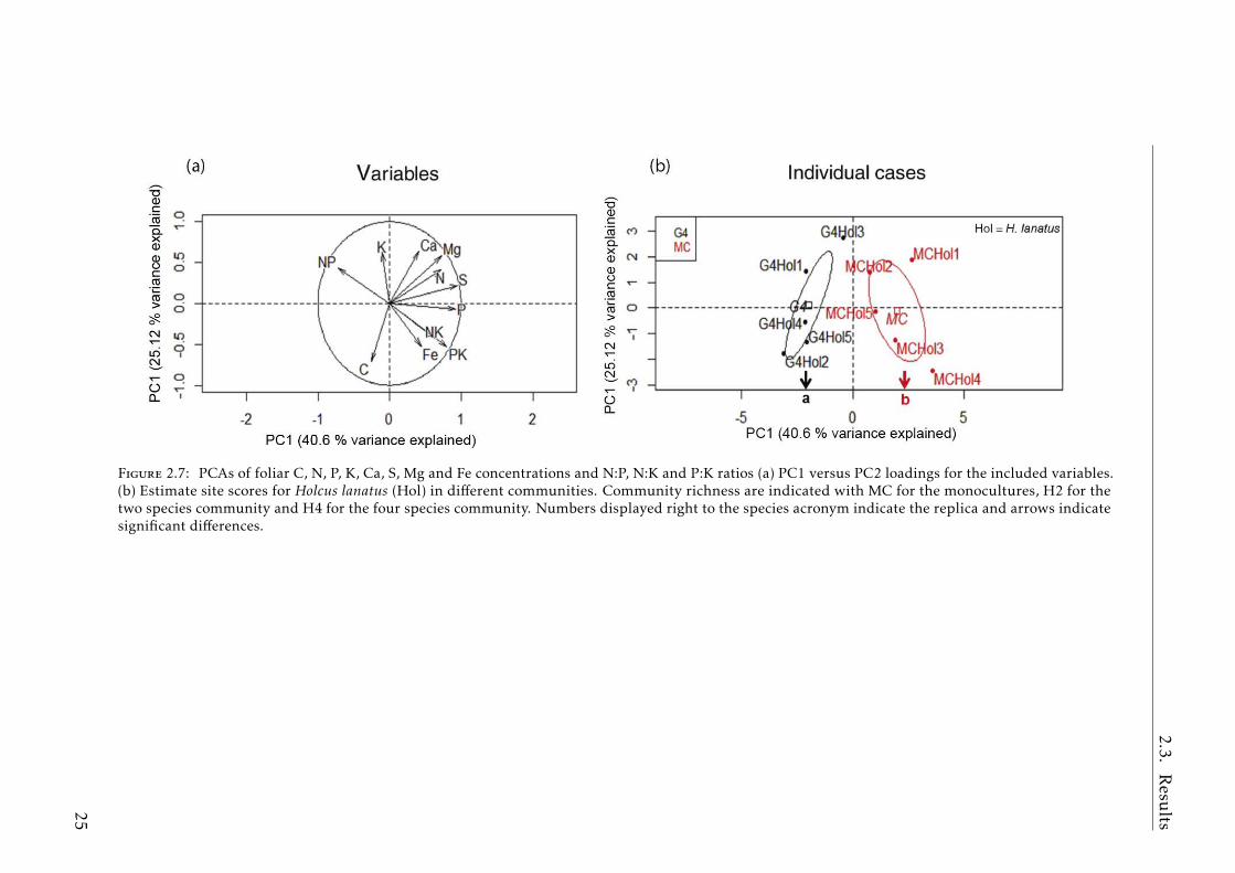
2.3.R
esults
Figure 2.7: PCAs of foliar C, N, P, K, Ca, S, Mg and Fe concentrations and N:P, N:K and P:K ratios (a) PC1 versus PC2 loadings for the included variables.(b) Estimate site scores for Holcus lanatus (Hol) in different communities. Community richness are indicated with MC for the monocultures, H2 for thetwo species community and H4 for the four species community. Numbers displayed right to the species acronym indicate the replica and arrows indicatesignificant differences.
25
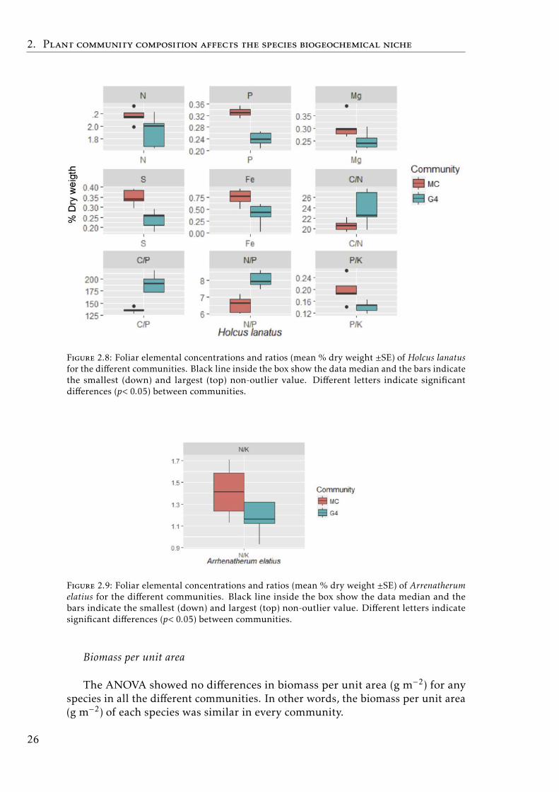
2. Plant community composition affects the species biogeochemical niche
Figure 2.8: Foliar elemental concentrations and ratios (mean % dry weight ±SE) of Holcus lanatusfor the different communities. Black line inside the box show the data median and the bars indicatethe smallest (down) and largest (top) non-outlier value. Different letters indicate significantdifferences (p< 0.05) between communities.
Figure 2.9: Foliar elemental concentrations and ratios (mean % dry weight ±SE) of Arrenatherumelatius for the different communities. Black line inside the box show the data median and thebars indicate the smallest (down) and largest (top) non-outlier value. Different letters indicatesignificant differences (p< 0.05) between communities.
Biomass per unit area
The ANOVA showed no differences in biomass per unit area (g m−2) for anyspecies in all the different communities. In other words, the biomass per unit area(g m−2) of each species was similar in every community.
26
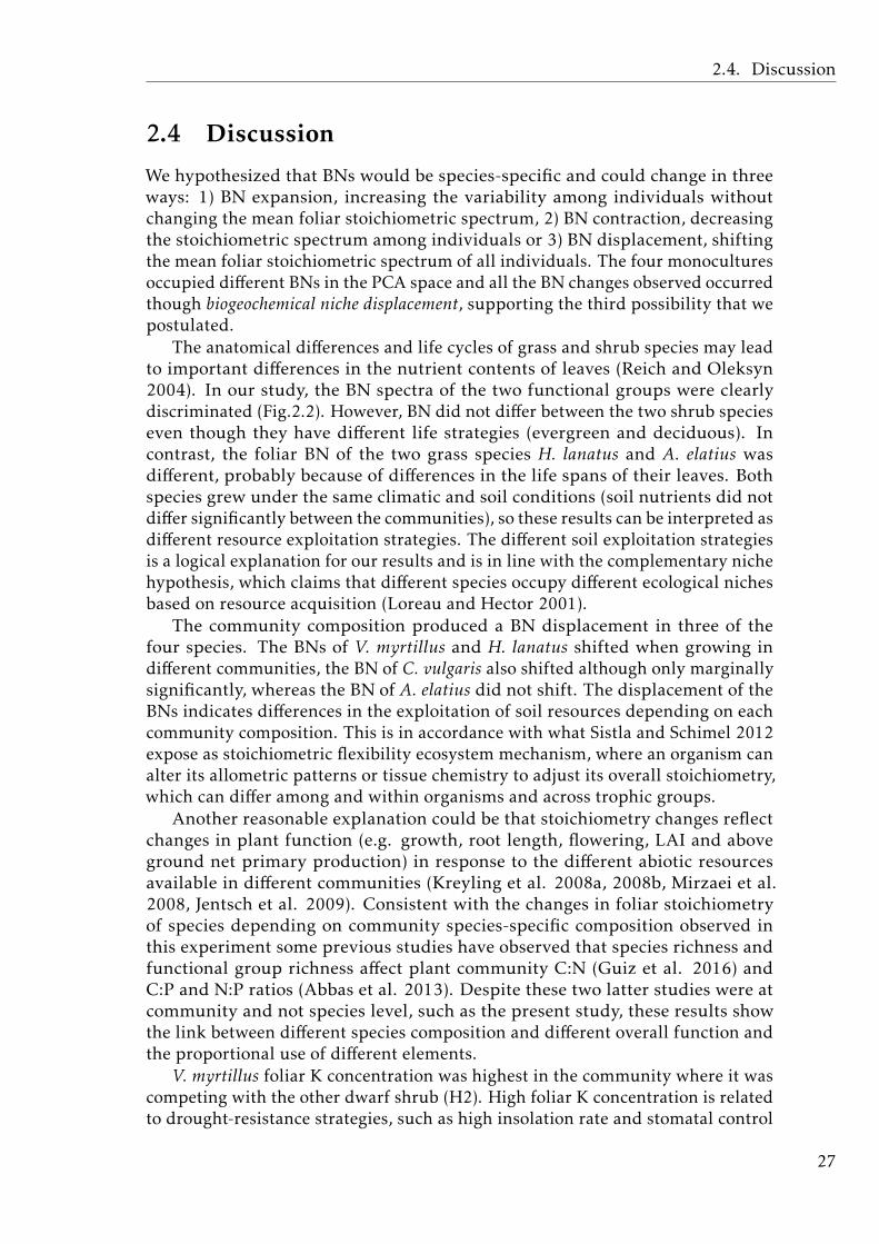
2.4. Discussion
2.4 Discussion
We hypothesized that BNs would be species-specific and could change in threeways: 1) BN expansion, increasing the variability among individuals withoutchanging the mean foliar stoichiometric spectrum, 2) BN contraction, decreasingthe stoichiometric spectrum among individuals or 3) BN displacement, shiftingthe mean foliar stoichiometric spectrum of all individuals. The four monoculturesoccupied different BNs in the PCA space and all the BN changes observed occurredthough biogeochemical niche displacement, supporting the third possibility that wepostulated.
The anatomical differences and life cycles of grass and shrub species may leadto important differences in the nutrient contents of leaves (Reich and Oleksyn2004). In our study, the BN spectra of the two functional groups were clearlydiscriminated (Fig.2.2). However, BN did not differ between the two shrub specieseven though they have different life strategies (evergreen and deciduous). Incontrast, the foliar BN of the two grass species H. lanatus and A. elatius wasdifferent, probably because of differences in the life spans of their leaves. Bothspecies grew under the same climatic and soil conditions (soil nutrients did notdiffer significantly between the communities), so these results can be interpreted asdifferent resource exploitation strategies. The different soil exploitation strategiesis a logical explanation for our results and is in line with the complementary nichehypothesis, which claims that different species occupy different ecological nichesbased on resource acquisition (Loreau and Hector 2001).
The community composition produced a BN displacement in three of thefour species. The BNs of V. myrtillus and H. lanatus shifted when growing indifferent communities, the BN of C. vulgaris also shifted although only marginallysignificantly, whereas the BN of A. elatius did not shift. The displacement of theBNs indicates differences in the exploitation of soil resources depending on eachcommunity composition. This is in accordance with what Sistla and Schimel 2012expose as stoichiometric flexibility ecosystem mechanism, where an organism canalter its allometric patterns or tissue chemistry to adjust its overall stoichiometry,which can differ among and within organisms and across trophic groups.
Another reasonable explanation could be that stoichiometry changes reflectchanges in plant function (e.g. growth, root length, flowering, LAI and aboveground net primary production) in response to the different abiotic resourcesavailable in different communities (Kreyling et al. 2008a, 2008b, Mirzaei et al.2008, Jentsch et al. 2009). Consistent with the changes in foliar stoichiometryof species depending on community species-specific composition observed inthis experiment some previous studies have observed that species richness andfunctional group richness affect plant community C:N (Guiz et al. 2016) andC:P and N:P ratios (Abbas et al. 2013). Despite these two latter studies were atcommunity and not species level, such as the present study, these results showthe link between different species composition and different overall function andthe proportional use of different elements.
V. myrtillus foliar K concentration was highest in the community where it wascompeting with the other dwarf shrub (H2). High foliar K concentration is relatedto drought-resistance strategies, such as high insolation rate and stomatal control
27
2. Plant community composition affects the species biogeochemical niche
(Sawhney and Zelitch 1969; Cakmak 2005; Sardans et al. 2012a; Sardans andPenuelas 2015a). Thus, high foliar K concentration in V. myrtillus growing in theH2 community suggest that the coexistence with C. vulgaris increased the waterstress on this species more than when it grew with grasses, or on its own in themonoculture. This could have happened because C. vulgaris has higher individualbiomass than the grass species and therefore demands more water.
H. lanatus nutrient concentrations were higher in the monoculture than in themixed stands, suggesting that interspecific competition was detrimental to itsnutrient uptake. Foliar element concentrations for A. elatius differed very littleamong the communities. The lack of stoichiometric flexibility in species that didnot change their BN indicate a more homeostatic stoichiometry, i.e. the abilityto maintain an specific elemental composition despite changes in the availabilityof elements in the surrounding environment (Elser et al. 2010; Yu et al. 2010).This type of stoichiometry could have important implications on the stability andprevalence of some species in changing environments.
Finally, our results provide good examples of the possible stoichiometric re-sponses of several species in different community conditions (displacement oftheir BN). The compromise between stoichiometric flexibility and homeostasisdetermined the differential responses of the species. However, this study lackedphysiological data that could explain the physiological mechanisms of these shifts.New and more thorough studies on foliar stoichiometry and community complex-ity, with a larger number of coexisting species and physiological measurementswill guaranteed enhance our knowledge about the stoichiometry of terrestrialsystem.
2.5 Conclusion
The study provides evidence that plant stoichiometry responds to changes inplant community composition. The BNs of the species changed in response tothe community composition in which they grew, and these changes occurred bydisplacement of their stoichiometry spectrum. Nevertheless, foliar compositionwas more homeostatic in C. vulgaris and especially in A. elatius. Regardless of theunderlying mechanisms ruling foliar stoichiometry changes, our results suggestthat changes in plant composition affect the species foliar stoichiometry. Ourresults are also a good example of a possible complementary BN hypothesis, andhighlight the importance of plant stoichiometric flexibility in the ecosystem. Weencourage further and deeper studies that contribute to better understanding therelationship between community composition and plant stoichiometry.
28
Encroachment of shrubs into subalpinegrasslands in the Pyrenees changes theplant-soil stoichiometry 3
29
3. Encroachment of shrubs into subalpine grasslands in the Pyrenees changes the
plant-soil stoichiometry
Abstract
Shrub encroachment has been reported over a large proportion of the subalpinegrasslands across Europe and is expected to have an important impact on thefunctioning and the biogeochemical cycle of these ecosystems. Shrubs and herba-ceous species differ in their growth forms, resource acquisitions and allocationstrategies, so the succession from grassland to shrubland is expected to causemajor changes in the plant-soil stoichiometry and cycling of nutrients in theecosystem. We investigated the stoichiometric changes in the soil and in the plantaboveground compartments of the main herbaceous species and shrubs involvedin this succession at two sites with contrasting abiotic and biotic conditions inthe Central Pyrenees.We analyzed the chemical composition (C, N, 15N, P, K,Ca, Mg and Fe) in the soil and in the plant compartments (leaves, leaf-litter andstems) of the main herbaceous species and shrubs at three contrasting stages ofthe succession from grassland to shrubland: grassland, young shrubland andmature shrubland. The plant-soil stoichiometry spectrum differed between thesuccessional stages. Shrub encroachment generally increased the C and Ca con-centration and the C:N ratio and often decreased the N, P and K concentrations inthe leaves and leaf-litter, while the concentrations of several soil nutrients (N, P,K Ca and Mg) mostly decreased. The stocks of C, N, P, Ca, and Mg in the totalaboveground biomass compartments increased with the advance of the encroach-ment. The stock of nutrients in the upper 10 cm in the soil was 100-fold largerthan in the biomass in all successional stages at North face and 100-fold largerin the grassland and young shrubland and 10-fold lager in the mature shrub-land at South face. Soil nutrient stocks mostly decreased along the succession atSouth face but not at North face.Shrub expansion into subalpine grassland has aclear impact on the plant-soil stoichiometry spectrum. The pure grassland is anecosystem dominated by hemicryoptophyte species with fast turnover of nutrientsbetween the plant compartments and the soil; the plant-soil system generallyshows high concentrations of N, P and K. The productivity of the grassland ishigh, but the stock of biomass is low. The expansion of shrubs, though, favoredthe dominance of long-lived species, with a more conservative strategy, with lowconcentrations of N and P in the plant-soil compartments and high C:nutrientratios in the aboveground biomass. The total stocks of C and nutrients in theaboveground biomass were nevertheless high because the biomass of the matureshrubland was very high compared to the grassland. We thus highlight the roleof shrubs in the sequestration of C and nutrients, through the allocation to theaboveground biomass. Moreover, shrub encroachment alters the strategy withwhich N is acquired, possibly through an increased uptake of N through ericoidor ectomycorrhizae. The changes in plant-soil elemental composition and stockssuggest a slowdown of the biogeochemical cycles in the subalpine mountain areaswhere shrub encroachment occurred.
• Key words: shrub encroachment, plant-soil stoichiometry, nutrient stocks,subalpine grassland succession, plant strategy.
30
3.1. Introduction
3.1 Introduction
The encroachment of shrub species into grasslands causes important changes inmany grass-dominated ecosystems at landscape and regional scales from low tohigh latitudes (Van Auken 2009, Myers-Smith et al. 2011, Naito and Cairns 2011,Komac et al. 2013, Formica et al. 2014). The expansion of shrubs is mostly causedby changes in climatic conditions and land use (Eldridge et al. 2011). For example,the ongoing increase in mean annual temperature and the thinning of permafrostat high latitudes are promoting the expansion of shrubs across the Arctic andsubarctic tundra (Tape et al. 2006; Hallinger et al. 2010; Myers-Smith et al. 2011).Shrub expansion has also been observed in most mountain ranges and massifsacross Europe at lower latitudes, where humans have used the subalpine andalpine grasslands for traditional activities such as extensive livestock herding(Roura-Pascual et al. 2005; Anthelme et al. 2007; Hallinger et al. 2010; Targettiet al. 2010; Ferre et al. 2013) for many centuries or even millennia (Gassiotand Jimenez 2006; Pelachs et al. 2007; Gassiot et al. 2016). The progressiveabandonment of these practices in recent decades has favored the encroachmentof shrubs into subalpine and alpine grasslands (MacDonald et al. 2000; Dullingeret al. 2003; Komac et al. 2013; Ameztegui et al. 2016). Climatic warming isalso expected to promote the expansion of woody species in subalpine and alpineregions in the Pyrenees (Grau et al. 2013; Penuelas et al. 2016; Angulo et al. 2019)and across Europe in the coming decades (Sanz-Elorza et al. 2003; Korner andPaulsen 2004; Wookey et al. 2009; IPCC 2013). The abandonment of subalpineand alpine grasslands is very apparent in the Pyrenees (northeastern IberianPeninsula), where traditional extensive livestock grazing and the frequency ofintentional fires to create or maintain pasture has substantially decreased in thelast century, mainly due to socio-economic changes in this area (Lasanta et al.2000; MacDonald et al. 2000; Serrano et al. 2000; Roura-Pascual et al. 2005;Jimenez and Pujol 2010; Barrio et al. 2013).
Shrub expansion is expected to cause several changes in ecosystem functioning,but few studies have focused on the impacts of expansion on the functioning ofsubalpine or alpine grasslands in the Pyrenees (Vitousek 1984; Montane et al.2007, 2010; Barrio et al. 2013; Catalan et al. 2017; Grau et al. 2019) andacross Europe (MacDonald et al. 2000; Wookey et al. 2009). Some studies havereported that shrub encroachment has increased the carbon (C) and nitrogen (N)concentrations in the soil and decreased soil pH (Knapp et al. 2008; Eldridge etal. 2011), but such changes may strongly depend on shrub traits and ecosystemfeatures. Shrub and grass species have contrasting growth forms and differ in manyfunctional traits of their adaptive and reproductive capacities and their strategiesof resource acquisition and allocation (Chapin and Korner 1994). Different co-occurring shrub species may also have contrasting traits and strategies (Illa etal. 2017), so the identity of shrubs is also crucial to understand the changes inecosystem functioning when encroachment occurs (Grau et al. 2019). Successionfrom grassland to shrubland is thus expected to cause important changes in thedistribution, cycling and stoichiometry of chemical elements in the plant-soilsystem. Furthermore, the increase in woody biomass during the succession addscomplexity to the persistence and cycling of C and nutrients in the ecosystem.
31
3. Encroachment of shrubs into subalpine grasslands in the Pyrenees changes the
plant-soil stoichiometry
Wood is highly persistent and stores C and nutrients such as N, phosphorus (P),potassium (K), calcium (Ca) and magnesium (Mg) (Chave et al. 2009; Sardans andPenuelas 2015b). The nutrient stocks stored in wood, however, depend mainly onwood density and may vary greatly among species (Sardans and Penuelas 2013;2015).
Most of the research on the impacts of shrub encroachment into grasslands hasfocused on soil C and N balances (Hibbard et al. 2001; Jackson et al. 2002; Hood etal. 2003; Throop and Archer 2008; Van-Auken 2009), including studies conductedin the Pyrenees (Garcia-Pausas et al. 2007; Montane et al. 2007; Garcia-Pausas2010). However, changes in the chemical composition of both plants and soils,including key elements such as P, K, Ca, Mg and iron (Fe), along the successionfrom grassland to shrubland, have not yet been investigated in detail. We studiedtwo common and contrasting landscapes where shrubs encroachment typicallyoccurs in the Pyrenees, one facing north (hereafter North face) and one facingsouth (hereafter South face). The two sites differ greatly in their abiotic conditions(macro and microclimate, bedrock lithology, topography) and in the functionalcharacteristics of their vegetation (biotic conditions); the dominant shrubs are:Calluna vulgaris (L.) Hull, Rhododendron ferrugineum L. and Vaccinium myrtillus L.at North face and Arctostaphylos uva-ursi (L.) Spreng, Juniperus communis L. andJuniperus sabina L. at South face. Each study site represents an independent casestudy because the grassland and shrubland species differ between the two sites. Ineach of the two sites, we established a replicated sampling design in three contrast-ing stages along the succession: a) the pure grassland (initial stage of succession,where shrubs are not yet present), b) the mixed, young shrubland (intermediatestage of succession, where grassland has small patches of shrubs) and c) the ma-ture shrubland (advanced stage of succession, where the dominant shrub speciesform large, monospecific patches). The main aim was to analyze the changes in thechemical composition (concentrations and stocks) of the aboveground-biomasscompartments (leaves and leaf-litter in herbaceous species; leaves, leaf-litter andstems in shrubs) and the soil along the succession from grassland to shrubland inthe Central Pyrenees.
A previous study conducted in the same study sites in the Pyrenees highlightedthat the concentrations of some soil nutrients (e.g. N, P or K) generally decreasedalong the succession from grassland to shrubland (Grau et al. 2019), althoughthere were differences between sites and shrub species. It was hypothesized thatshrubs may store nutrients in the biomass to take control of nutrients of theecosystem and promote their further expansion along the succession. In thiscurrent study, we test this hypothesis and investigate whether the decrease in theconcentrations of soil nutrients along the succession was coupled with changes inconcentrations and/or stocks of nutrients in the aboveground biomass and in thesoil. Moreover, shrub expansion into grassland is expected to shape the plant-soilstoichiometry spectrum and the biogeochemical cycle through changes in theabiotic and biotic conditions along the succession from grassland to shrubland.We thus hypothesized that each successional stage would show a contrasting plant-soil stoichiometric spectrum, resulting from changes in vegetation structure andallocation strategies in each stage, and that C:nutrient ratios in the abovegroundbiomass and soil would increase over the succession due to the lignification of
32
3.2. Material & Methods
plant compartments.
3.2 Material & Methods
Study area, species and sampling design
The two study sites were located in the Central Pyrenees (NE Iberian penin-sula), one site on the North face (Bargadera, Val d’Aran, 42°3953.9N, 00°5007.8E,with Cambro-Ordovician schists, sandstones and quartzites) and one on the Southface (Fogueruix, Pallars Sobira, 42°3532.9N, 01°0428.8E, with a Devonian slatylimestone), both on the periphery of the ‘Aiguestortes i Estany de Sant Maurici’National Park (Fig.A.3.1). The two sites are separated by only 22 km but arecharacterized by contrasting macro and microclimates; the site in Val d’Aran hasa strong Atlantic influence, whereas the site in Pallars Sobira is more continental.The mean annual number of days with precipitation or fog and the relative airhumidity are therefore higher at North face than South face (Catalan Meteoro-logical Service, http://meteo.cat/wpweb/climatologia, accessed on March 2018).The North face is a smooth north-facing slope at an altitude of 1800-1900 m a.s.l.Since 2015, annual precipitation at the nearest meteorological station to Northface (Bagergue, 1400 m a.s.l.) has ranged from 800 to 900 mm, mean annualtemperature has ranged from 8 to 9 °C and minimum and maximum absolutetemperatures were -14 and 30 °C, respectively. The South face site is a steep south-facing slope at an altitude of 2000-2100 m a.s.l. Since 2015, annual precipitationat the nearest meteorological station to South face (Planes de Son, 1540 m a.s.l.)has ranged from 600 to 800 mm, mean annual temperature has ranged from 8to 10 °C and minimum and maximum absolute temperatures were -15 and 30°C, respectively. Both meteorological stations are at altitudes (ca. 400 m) lowerthan the study sites, so precipitation is expected to be higher and temperaturesare expected to be lower (average and range) than the reported values at bothsites. Both sites are in areas that have been intensively used for livestock grazingfor many centuries, but socio-economic changes in the Pyrenees since the 1950sdecreased the density of livestock, and some summer pastures have been aban-doned (MacDonald et al. 2000; Jimenez and Pujol 2010), which have favored theexpansion of shrubs into these former grasslands.
The grassland at North face is classified as a mesophilic, dense subalpine grass-land ‘Nardion’(Galvanek and Janak 2008), dominated mostly by grasses (Festucaeskia Ramond ex DC. and Festuca nigrescens Lam.) with scarcer forbs (Trifoliumalpinum L., and Cerastium arvense L.). The succession is mostly driven by thedwarf shrubs Calluna vulgaris, Rhododendron ferrugineum and Vaccinium myrtillus.The grassland at South face is classified as a xerophilic, open montane grassland‘Xerobromion’ (Carreras et al. 1983; EAE 2019), dominated by grasses (Festucaovina L. and Festuca gautieri (Hack.) K.Richt) that co-occur with small forbs (suchas Hieracium pilosella L., Achillea millefolium L. and Potentilla neumanniana Rchb.).The succession from grassland to shrubland is mostly driven by the dwarf shrubsArctostaphylos uva-ursi, Juniperus communis and Juniperus sabina L. and to a muchlesser extent by Helianthemum nummularium (L.) Mill. or Thymus pulegioides L.
33
3. Encroachment of shrubs into subalpine grasslands in the Pyrenees changes the
plant-soil stoichiometry
Soils at the North face site are built from Cambro-Ordovician schists, sand-stone and quartzite, and, given the moderate slope of the area, they are moderatelydeep, rich in organic matter, and acidic, corresponding in general to Humudepts.Those at the South face site result mainly from Silurian pelite and also fromDevonian lime-rich slate. Being this site steeper, soils are shallower and irregu-lar, moderately acidic and humic, broadly corresponding to lithic Humudepts(Boixadera et al. 2014). Moreover, soils at the South face experience summerdrought episodes resulting into apparent drying off of the shallow soil level, whichdoes not occur at the North face. The soil pH in the North face tend be moreacidic (pH around 4.7-5) than in South face (pH 5.7-6.3) (Grau et al. 2019). Thepercentage of soil organic matter measured in the same study sites were higherat North face (herbaceous species: 21.2%, Calluna vulgaris: 37.8%, Rhododendronferrugineum: 40.12% and Vaccinium myrtillus 40.6%) than South face (herbaceousspecies: 16.5%, Arctostaphylos uva-ursi: 16.2%, Juniperus communis:13.2% andJuniperus sabina: 13.4%) (Grau et al. 2019).
We selected three stages at each site along the succession from grasslandto shrubland: a) pure grassland, which is still regularly grazed by domesticanimals (Oriol Grau, pers. observation), is dominated by herbaceous speciesand has no shrubs, b) young shrubland, composed of a mosaic of herbaceousspecies and shrub patches of ca. 1-2 m2 and c) mature shrubland, where thedominant shrub species form large monospecific patches (at least 10 × 10 m). Weselected the most common shrubs at each site (C. vulgaris, R. ferrugineum and V.myrtillus at North face and A. uva-ursi, J. communis and J. sabina at South face(see suplementary Table A.3.1, A.3.2 and A.3.3 for the ecological and functionalcharacterization of the shrub species studied). The herbaceous species and eachof the shrubs occurring along the succession in each site will hereafter be referredto as ‘vegetation types’.
The replication of the successional stages was done in each site separately; thetwo sites were not treated as replicates in the analyses but as two independentstudy cases. Sampling plots were established to reproduce the extant structureof the vegetation in each successional stage. We established four replicate 2 × 2m plots (separated by a minimum of 10 m) in the pure grassland, and in each ofthree mature shrublands at each site. In the mixed shrubland, though, the plotsfor each vegetation type (grass, shrub 1, shrub 2, shrub 3) were grouped becauseall vegetation types co-occurred; in this intermediate stage, we established fourgroups of four plots (Fig.A.3.2 and Grau et al. 2019 for further details). In totalwe sampled 32 plots per site along the succession from pure grassland to matureshrubland. The distance between the successional stages or among the matureshrublands of each shrub species was >100 m. The plots in the pure grasslandwere placed in areas that represented the mixture of grass species that co-occurredin this successional stage, whereas the plots in the mature shrubland were placedin large patches dominated by each of the shrub species.
We collected plant and soil samples towards the end of the growing season(September 2015) for the analysis of their elemental compositions. The litterlayer was removed prior to the soil sampling; root samples could not be collectedand analyzed in this study. We collected a total of 144 shrub samples: 2 sites ×2 successional stages where shrubs were present (young shrubland and mature
34
3.2. Material & Methods
shrubland) × 3 shrub species × 4 replicates × 3 plant compartments (leaves, leaf-litter -dead leaves still attached to the plant- and stems). We collected a total of 32samples of herbaceous species in the pure grassland and the young shrubland: 2sites × 2 successional stages where these were present (pure grassland and youngshrubland) × 4 replicates × 2 plant compartments (leaves and leaf-litter). We alsocollected soil samples to a depth of 10 cm next to each plant sample with a 5-cmdiameter soil corer, 48 samples for shrubs (2 sites x 2 successional stages x 3 shrubsspecies x 4 replicas) and 16 samples for herbaceous species (2 sites x 2 successionalstages x 1 grassland x 4 replicas), for a total of 64 soil samples. The concentrationsof C, N, P, K, Mg, Ca and Fe (see details of the chemical analyses in the nextsection) and15N were measured in leaves, leaf-litter, lignified stems and soils. Thesamples were transported to the laboratory in paper envelopes, the soil sampleswere sieved (2 mm) and all samples were oven-dried at 60 °C for 48 h. Theywere then ground with a ball mill (Retsch, model MM400. RestchGmbH. Haan,Germany), weighed with an AB204 Mettler Toledo (Mettler Toledo, Barcelona,Spain) and analyzed in the chemistry laboratories at Servei d’Analisi Quımica,Autonomous University of Barcelona (Barcelona, Spain), where the percentagesof P, K, Mg, Ca and Fe in dry weight were determined, and at the University ofCalifornia Davis Isotope Facility (Davis, USA), where the isotopic compositions(δ15N) and percentages of C and N in dry weight were determined.
We revisited the same sampling areas in September 2016 and collected moresamples to characterize the mean biomass of each plant compartment and thebulk density of the soil, which we used to estimate the stocks of C and nutrientsin the aboveground compartments (g m−2) of the vegetation types and the soil.We assumed that the aboveground biomass of the herbaceous species was similarbetween the two years, because their aboveground structures are entirely or nearlynewly produced each year and the climatic conditions (mean annual temperatureand precipitation) did not vary much (http://meteo.cat/wpweb/climatologia).The changes in biomass of shrubs are very limited in this ecosystem (Ninot et al.2010a), so we do not expect large significant variations between two consecutiveyears with similar climatic conditions. We collected the aboveground vegetationwithin 25 × 25 cm quadrats in the young shrubland and 50 × 50 cm quadrats inthe pure grassland and mature shrubland. The biomass was then transported inplastic bags to the laboratory and sorted manually into leaves and woody stems(only for shrubs). We collected a total of 48 foliar samples and 48 stem samplesfrom shrubs (2 sites × 2 successional stages where shrubs were present × 3 shrubspecies × 4 replicates) and 16 foliar samples from herbaceous species (2 sites × 2successional stages where herbaceous species were present × 4 replicates). Theplant material was sorted and oven-dried at 60 °C to a constant weight, and thedry weight was measured. We collected soil samples with a bulk-density corer (9cm diameter to a depth of 10 cm) to estimate the bulk density for each vegetationtype. The quantity of soil (g cm−2) was calculated as the product of the bulkdensity multiplied by the core depth. We also calculated the annual leaf-litterproduction based on estimates of foliar persistence conducted in nearby locations(Ninot et al. unpublished data). Leaf-litter productivity was used to estimate theannual input of nutrients from the leaf-litter for each vegetation type.
35
3. Encroachment of shrubs into subalpine grasslands in the Pyrenees changes the
plant-soil stoichiometry
Chemical analyses
The concentrations of C, N (dry weight (dw)/dry weight) and 15N isotope weredetermined by gas chromatography. The amount of sample used was based on thepercentages of C and N in each type of sample. For leaves, leaf-litter and stems,4.5 mg of dry sample were weighed and encapsulated in tin capsules. For soils,8.6 mg of each sample were used. The samples were then analyzed for C andN with an Elementar Cube system (Elementar Analyzen system GmbH, Hanau,Germany). 15N isotope was analyzed by an Elementar Vario EL Cube or MicroCube elemental analyzer connected to a PDZ Europa 20-20 isotope-ratio massspectrometer (Sercon Ltd., Cheshire, UK). The plant samples were combustedat 1000°C in a reactor packed with chromium oxide and silvered copper oxideand soils were combusted at 1080 °C in a reactor packed with copper oxide andtungsten (VI) oxide. The oxides were then removed in a reduction reactor (reducedcopper at 650 °C). The samples were interspersed during the analysis with severalreplicates of at least two laboratory standards. These standards, which wereselected for their compositional similarity to the samples, had been previouslycalibrated against National Institute of Standards and Technology (NIST) StandardReference Materials (IAEA-N1, IAEA-N2, IAEA-N3, USGS-40 and USGS-41).Preliminary isotopic ratios were measured relative to the reference gases analyzedfor each sample. These preliminary ratios were refined by correcting for the entirebatch based on the known ratios of the laboratory standards. The long-termstandard deviation was 0.3‰ for δ15N.
The concentrations of P, Mg, K, Ca and Fe in the leaves, leaf-litter, stems andsoil were determined by inductively coupled plasma mass spectrometry (ICP-MS)after digestion. For leaves, leaf-litter and stems, 0.25g of dry material were dilutedin 5 ml of concentrated HNO3 and digested in a MARSXpress microwave system(CEM GmbH, Kamp-Lintfort, Germany). The solution generated was analyzed byICP-MS to determine the elemental concentrations. The accuracy of the biomassdigestions and analytical procedures was assessed using certified biomass NIST1573a (tomato leaf, NIST, Gaitherburg, USA) standards and regularly analyzingblank solutions with no sample (5 mL of HNO3 and 2 mL of H2O2 with no sample).Dry soil subsamples of 0.1 g were dissolved in an acidic mixture of HNO3, HCland HF and digested as described for the plant samples. The solutions were di-luted with 1% HNO3 (v/v) before injection into the spectrometer. Blank solutions(5 mL of HNO3 and 2 mL of H2O2 with no sample) were regularly analyzed. Totalstocks of the elements (g m−2) for each plant compartment and the soil werecalculated as the biomass (leaves, leaf-litter or stems) and soil weights multipliedby the concentration of each element analyzed. The C:N, C:P and N:P ratios werecalculated on a mass basis.
Statistical analyses
We conducted principal component analyses (PCAs) of the elements to visu-alize the overall differences in the chemical composition of the plant and soilsamples collected for each vegetation type (shrub and herbaceous species) andsuccessional stage. We standaridzed the variables before the analyses. We per-
36
3.2. Material & Methods
formed a PCA for the elements of all compartments (leaves, leaf-litter and soil) foreach site separately to assess the differences in the chemical compositions amongthe successional stages and vegetation types within each site. If two variables werehighly positively correlated (Pearson’s product moment correlation coefficient>0.6), we excluded one of the two in the PCA to avoid the overfitting of variables.We also conducted PCAs of each plant compartment (leaves, leaf-litter, and stems)and soil using data from both study sites to identify differences between vegetationtypes and sites. To identify links between the functional traits of the shrubs andthe foliar elements concentrations (C, N, P, K, Mg, Ca and Fe), we conducted PCAsof the foliar elemental concentrations and some key functional measurements, asseed weight, specific leaf area (SLA), wood density, biomass per unit area, heightand annual leaf-litter production. All PCAs were conducted with the ‘ggbiplot’(Wickham 2009) and ‘FactoMineR’ (Le et al. 2008) packages in R. The significanceof the differences between vegetation types and successional stages in each PCAwere tested by permutational multivariate analyses of variance (PERMANOVAs)with the R ‘vegan’ package (Oksanen et al. 2017). β dispersion homogeneity testswere conducted prior to PERMANOVA analyses. We analysed the differences inelemental concentrations (dry weight (dw) of nutrient/dw of sample × 100) andstocks (g m−2) in the plant and soil and between vegetation types (herbaceousspecies and shrub 1, shrub 2, and shrub 3) and successional stages at each site.Although in our sampling design we maximised the independence of samples asmuch as possible given the extant structure of vegetation along the succession, itwas not possible to find a completely independent, random distribution of com-binations of successional stage × vegetation type in the field sites. We thereforefirstly checked if there were any underlying patterns of spatial aggregation inour data with autocorrelation semivariograms (‘nlme’ package, (Pinheiro et al.2017)), that are used for measuring the degree of spatial dependence betweenobservations as a function of distance. As in Grau et al. (2019) the initial visualinterpretation of the semivariograms indicated that in most cases the data wasnot autocorrelated despite the plots were not completely randomized. Yet, wepreferred to statistically check if autocorrelation should be accounted for in themodels. To do so we built two types of models: 1) Generalised least square (GLS)models that did not account for spatial autocorrelation, 2) GLS models that in-cluded the ‘corSpatial’ R function to account for potential spatial autocorrelation.For this second type of GLS models, the coordinates (longitude and latitude)of each plot were specified and we fitted five different models using a differentautocorrelation structure each time (e.g. exponential, linear, gaussian, rationalquadratic or spherical). After running all the models (one without and five withautocorrelation structure) for the element concentrations and stocks in each soilor plant compartment, we compared and selected the best model using scores ofthe Akaike Information Criterion (AIC). We used maximised log-likelihood in allcases and checked the normal distribution of the data before run the models. Thepure grassland was the initial stage of the succession from grassland to shrubland,and we considered it as the reference level in all models. The two study sites wereanalyzed as two independent study cases, so ‘site’ was not included in the modelsas a factor. All analyses were performed with R 3.2.4 (RCoreTeam 2017).
37
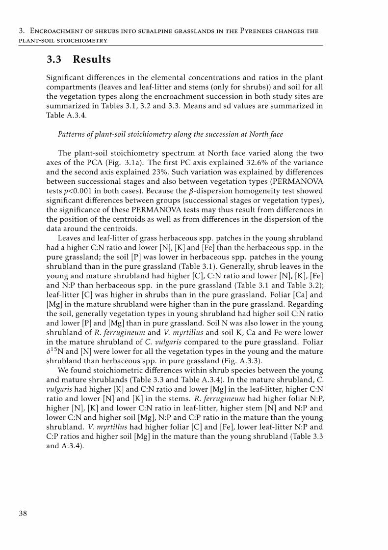
3. Encroachment of shrubs into subalpine grasslands in the Pyrenees changes the
plant-soil stoichiometry
3.3 Results
Significant differences in the elemental concentrations and ratios in the plantcompartments (leaves and leaf-litter and stems (only for shrubs)) and soil for allthe vegetation types along the encroachment succession in both study sites aresummarized in Tables 3.1, 3.2 and 3.3. Means and sd values are summarized inTable A.3.4.
Patterns of plant-soil stoichiometry along the succession at North face
The plant-soil stoichiometry spectrum at North face varied along the twoaxes of the PCA (Fig. 3.1a). The first PC axis explained 32.6% of the varianceand the second axis explained 23%. Such variation was explained by differencesbetween successional stages and also between vegetation types (PERMANOVAtests p<0.001 in both cases). Because the β-dispersion homogeneity test showedsignificant differences between groups (successional stages or vegetation types),the significance of these PERMANOVA tests may thus result from differences inthe position of the centroids as well as from differences in the dispersion of thedata around the centroids.
Leaves and leaf-litter of grass herbaceous spp. patches in the young shrublandhad a higher C:N ratio and lower [N], [K] and [Fe] than the herbaceous spp. in thepure grassland; the soil [P] was lower in herbaceous spp. patches in the youngshrubland than in the pure grassland (Table 3.1). Generally, shrub leaves in theyoung and mature shrubland had higher [C], C:N ratio and lower [N], [K], [Fe]and N:P than herbaceous spp. in the pure grassland (Table 3.1 and Table 3.2);leaf-litter [C] was higher in shrubs than in the pure grassland. Foliar [Ca] and[Mg] in the mature shrubland were higher than in the pure grassland. Regardingthe soil, generally vegetation types in young shrubland had higher soil C:N ratioand lower [P] and [Mg] than in pure grassland. Soil N was also lower in the youngshrubland of R. ferrugineum and V. myrtillus and soil K, Ca and Fe were lowerin the mature shrubland of C. vulgaris compared to the pure grassland. Foliarδ15N and [N] were lower for all the vegetation types in the young and the matureshrubland than herbaceous spp. in pure grassland (Fig. A.3.3).
We found stoichiometric differences within shrub species between the youngand mature shrublands (Table 3.3 and Table A.3.4). In the mature shrubland, C.vulgaris had higher [K] and C:N ratio and lower [Mg] in the leaf-litter, higher C:Nratio and lower [N] and [K] in the stems. R. ferrugineum had higher foliar N:P,higher [N], [K] and lower C:N ratio in leaf-litter, higher stem [N] and N:P andlower C:N and higher soil [Mg], N:P and C:P ratio in the mature than the youngshrubland. V. myrtillus had higher foliar [C] and [Fe], lower leaf-litter N:P andC:P ratios and higher soil [Mg] in the mature than the young shrubland (Table 3.3and A.3.4).
38
3.3.R
esults
Figure 3.1: Principal component analysis (PCA) based on the chemical elements (C, N, P, K, Ca, Mg and Fe) in leaves (lf), leaf-litter (ltt) and soil for thesuccessional stages and vegetation types at (a) North face and (b) South face. Only variables that were poorly correlated with each other (Pearson’s coefficients< 0.6) are included in the analyses. Different colors indicate the successional stages and different shapes indicate the vegetation types. The ellipses representthe dispersion around the centroid for each successional stage with a normal probability of 0.85.
39
3. Encroachment of shrubs into subalpine grasslands in the Pyrenees changes the
plant-soil stoichiometry
The stocks of nutrients were generally much larger in the soil (generally 100-fold in all successional stages) than in the biomass. The stocks of N (9.4 g m−2), P(0.71 g m−2), K (8.5 g m−2) and Fe (0.06 g m−2) in herbaceous spp. leaves in thepure grassland were significantly larger than in the leaves of all vegetation typesin the young and mature shrublands (Fig. 3.2. Table A.3.4). Nevertheless, shrubstems generally stored larger amounts of C and nutrients compared to leaves, sothat the stocks of C and nutrients in the aboveground biomass in the young andmature shrubland were generally much larger than in the grassland (except forK). C. vulgaris and R. ferrugineum in the mature shrubland had higher stocks ofsoil C (8953.5 g m−2, 7388.7 g m−2, respectively) and soil N (507.5 g m−2, only C.vulgaris) than the pure grassland (C: 3645.7 g m−2, N: 294.7 g m−2). The stocksof soil P and K stocks in C. vulgaris in the mature shrubland tend to increase butnot significantly. Herbaceous spp. in pure grassland showed the highest annualleaf-litter production (509.4 g m−2 year−1) (Fig. A.3.4 and Table A.3.4); also, theannual leaf-litter production in V. myrtillus was higher in the mature (99.8 g m−2
year−1) than the young shrubland (53.8 g m−2 year−1) (Fig. A.3.4 and Table A.3.4),implying higher inputs of C (49.5 g m−2 year−1), N (1.1 g m−2 year−1), P (0.12 gm−2 year−1), K (0.68 g m−2 year−1), Mg (0.2 g m−2 year−1), Ca (0.7 g m−2 year−1)and Fe (0.007g m−2 year−1) in the mature shrubland (Fig. A.3.4 and Table A.3.4).Leaf-litter production did not differ significantly for the other vegetation types.
Patterns of plant-soil stoichiometry along the succession at South face
The plant-soil stoichiometry spectrum at South face varied greatly along thetwo axes of the PCA based on the chemical composition of leaves, leaf-litter andsoil (Fig. 3.1b). The first PC axis explained 30.7% of the variance, and the secondPC axis explained 20.1%. We found significant differences between successionalstages (PERMANOVA p<0.001) and vegetation types (PERMANOVA p<0.004). Ingeneral, herbaceous spp. in the young shrubland had lower [N] and [K] in leaves,higher [C], [Fe], N:P and C:N ratio and lower [N] and [P] in the leaf-litter andhigher [Fe] and lower [N], [Ca] and [Mg] in soil than the pure grassland (Tables 3.1and A.3.4). Shrub leaves in the young shrubland generally had higher [C] and C:Nratios and lower [N], [K] and N:P ratio than herbaceous spp. in pure grassland,and shrub leaf-litter generally had higher [C] and lower [N] than herbaceous spp.in pure grassland (Table 3.2). The soil for all vegetation types in young shrublandhad lower [N], [Ca], [Mg] and N:P ratio than the soil in herbaceous spp. in puregrassland. Leaves in the mature shrubland often had higher [Ca] and [Mg] andlower [N], [K] and N:P ratio, and leaf-litter with higher [C] and lower [Fe] thanthe pure grassland. Soil [N], [Ca], [Mg] were always lower in the young shrublandthan the pure grassland (Table 3.1); soil [P] was also lower in the mature shrublandof A. uva-ursi and J. sabina. (Table 3.2). Foliar δ15N and [N] were also lower for allvegetation types in the young and the mature shrubland than herbaceous spp. inpure grassland (Fig. A.3.3), as observed at North face.
40
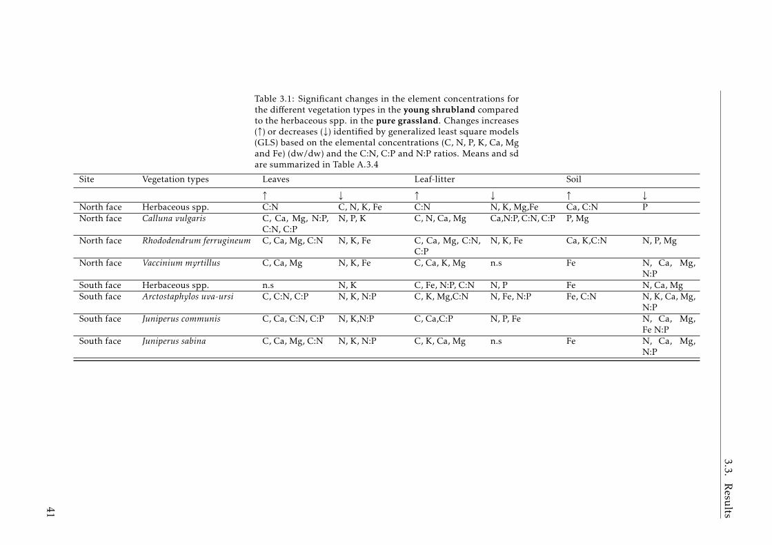
3.3.R
esults
Table 3.1: Significant changes in the element concentrations forthe different vegetation types in the young shrubland comparedto the herbaceous spp. in the pure grassland. Changes increases(↑) or decreases (↓) identified by generalized least square models(GLS) based on the elemental concentrations (C, N, P, K, Ca, Mgand Fe) (dw/dw) and the C:N, C:P and N:P ratios. Means and sdare summarized in Table A.3.4
Site Vegetation types Leaves Leaf-litter Soil
↑ ↓ ↑ ↓ ↑ ↓North face Herbaceous spp. C:N C, N, K, Fe C:N N, K, Mg,Fe Ca, C:N PNorth face Calluna vulgaris C, Ca, Mg, N:P,
C:N, C:PN, P, K C, N, Ca, Mg Ca,N:P, C:N, C:P P, Mg
North face Rhododendrum ferrugineum C, Ca, Mg, C:N N, K, Fe C, Ca, Mg, C:N,C:P
N, K, Fe Ca, K,C:N N, P, Mg
North face Vaccinium myrtillus C, Ca, Mg N, K, Fe C, Ca, K, Mg n.s Fe N, Ca, Mg,N:P
South face Herbaceous spp. n.s N, K C, Fe, N:P, C:N N, P Fe N, Ca, MgSouth face Arctostaphylos uva-ursi C, C:N, C:P N, K, N:P C, K, Mg,C:N N, Fe, N:P Fe, C:N N, K, Ca, Mg,
N:PSouth face Juniperus communis C, Ca, C:N, C:P N, K,N:P C, Ca,C:P N, P, Fe N, Ca, Mg,
Fe N:PSouth face Juniperus sabina C, Ca, Mg, C:N N, K, N:P C, K, Ca, Mg n.s Fe N, Ca, Mg,
N:P
41
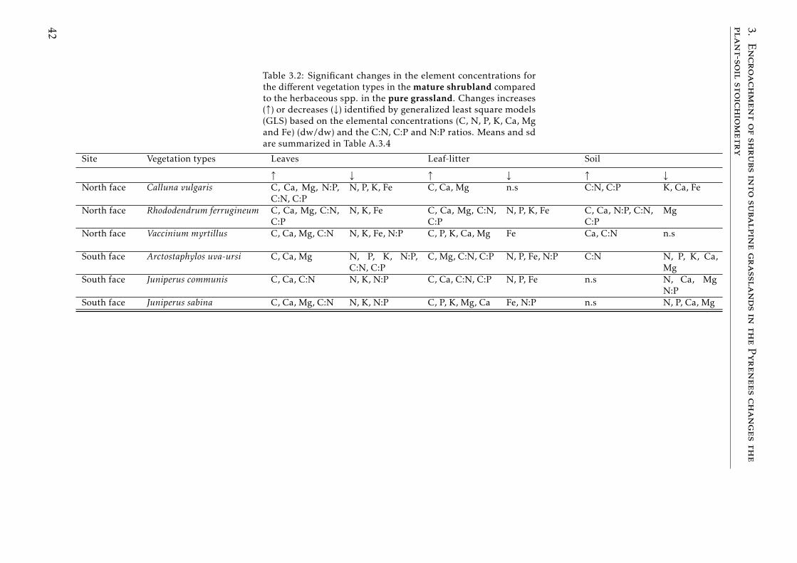
3.EncroachmentofshrubsintosubalpinegrasslandsinthePyreneeschangesthe
plant-soilstoichiometry
Table 3.2: Significant changes in the element concentrations forthe different vegetation types in the mature shrubland comparedto the herbaceous spp. in the pure grassland. Changes increases(↑) or decreases (↓) identified by generalized least square models(GLS) based on the elemental concentrations (C, N, P, K, Ca, Mgand Fe) (dw/dw) and the C:N, C:P and N:P ratios. Means and sdare summarized in Table A.3.4
Site Vegetation types Leaves Leaf-litter Soil
↑ ↓ ↑ ↓ ↑ ↓North face Calluna vulgaris C, Ca, Mg, N:P,
C:N, C:PN, P, K, Fe C, Ca, Mg n.s C:N, C:P K, Ca, Fe
North face Rhododendrum ferrugineum C, Ca, Mg, C:N,C:P
N, K, Fe C, Ca, Mg, C:N,C:P
N, P, K, Fe C, Ca, N:P, C:N,C:P
Mg
North face Vaccinium myrtillus C, Ca, Mg, C:N N, K, Fe, N:P C, P, K, Ca, Mg Fe Ca, C:N n.s
South face Arctostaphylos uva-ursi C, Ca, Mg N, P, K, N:P,C:N, C:P
C, Mg, C:N, C:P N, P, Fe, N:P C:N N, P, K, Ca,Mg
South face Juniperus communis C, Ca, C:N N, K, N:P C, Ca, C:N, C:P N, P, Fe n.s N, Ca, MgN:P
South face Juniperus sabina C, Ca, Mg, C:N N, K, N:P C, P, K, Mg, Ca Fe, N:P n.s N, P, Ca, Mg
42
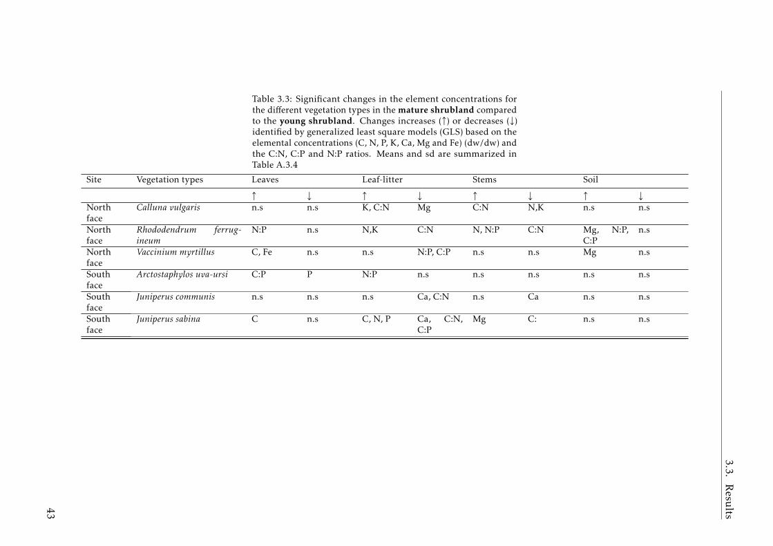
3.3.R
esults
Table 3.3: Significant changes in the element concentrations forthe different vegetation types in the mature shrubland comparedto the young shrubland. Changes increases (↑) or decreases (↓)identified by generalized least square models (GLS) based on theelemental concentrations (C, N, P, K, Ca, Mg and Fe) (dw/dw) andthe C:N, C:P and N:P ratios. Means and sd are summarized inTable A.3.4
Site Vegetation types Leaves Leaf-litter Stems Soil
↑ ↓ ↑ ↓ ↑ ↓ ↑ ↓Northface
Calluna vulgaris n.s n.s K, C:N Mg C:N N,K n.s n.s
Northface
Rhododendrum ferrug-ineum
N:P n.s N,K C:N N, N:P C:N Mg, N:P,C:P
n.s
Northface
Vaccinium myrtillus C, Fe n.s n.s N:P, C:P n.s n.s Mg n.s
Southface
Arctostaphylos uva-ursi C:P P N:P n.s n.s n.s n.s n.s
Southface
Juniperus communis n.s n.s n.s Ca, C:N n.s Ca n.s n.s
Southface
Juniperus sabina C n.s C, N, P Ca, C:N,C:P
Mg C: n.s n.s
43
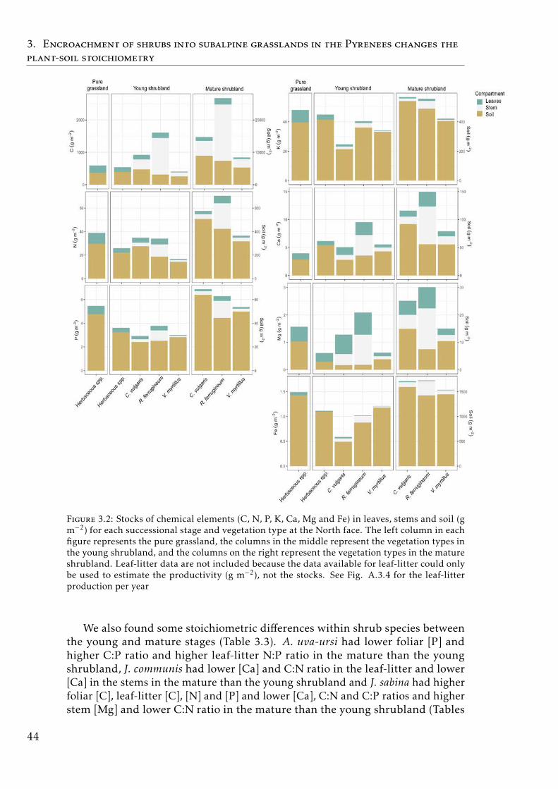
3. Encroachment of shrubs into subalpine grasslands in the Pyrenees changes the
plant-soil stoichiometry
Figure 3.2: Stocks of chemical elements (C, N, P, K, Ca, Mg and Fe) in leaves, stems and soil (gm−2) for each successional stage and vegetation type at the North face. The left column in eachfigure represents the pure grassland, the columns in the middle represent the vegetation types inthe young shrubland, and the columns on the right represent the vegetation types in the matureshrubland. Leaf-litter data are not included because the data available for leaf-litter could onlybe used to estimate the productivity (g m−2), not the stocks. See Fig. A.3.4 for the leaf-litterproduction per year
We also found some stoichiometric differences within shrub species betweenthe young and mature stages (Table 3.3). A. uva-ursi had lower foliar [P] andhigher C:P ratio and higher leaf-litter N:P ratio in the mature than the youngshrubland, J. communis had lower [Ca] and C:N ratio in the leaf-litter and lower[Ca] in the stems in the mature than the young shrubland and J. sabina had higherfoliar [C], leaf-litter [C], [N] and [P] and lower [Ca], C:N and C:P ratios and higherstem [Mg] and lower C:N ratio in the mature than the young shrubland (Tables
44
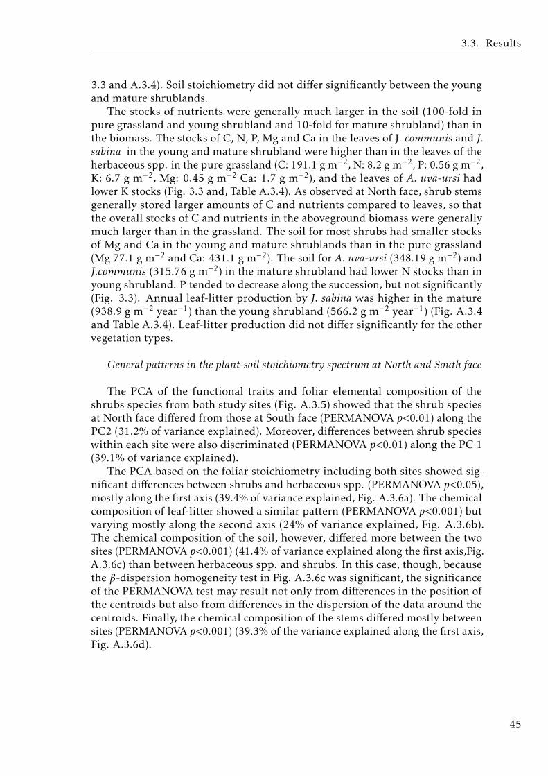
3.3. Results
3.3 and A.3.4). Soil stoichiometry did not differ significantly between the youngand mature shrublands.
The stocks of nutrients were generally much larger in the soil (100-fold inpure grassland and young shrubland and 10-fold for mature shrubland) than inthe biomass. The stocks of C, N, P, Mg and Ca in the leaves of J. communis and J.sabina in the young and mature shrubland were higher than in the leaves of theherbaceous spp. in the pure grassland (C: 191.1 g m−2, N: 8.2 g m−2, P: 0.56 g m−2,K: 6.7 g m−2, Mg: 0.45 g m−2 Ca: 1.7 g m−2), and the leaves of A. uva-ursi hadlower K stocks (Fig. 3.3 and, Table A.3.4). As observed at North face, shrub stemsgenerally stored larger amounts of C and nutrients compared to leaves, so thatthe overall stocks of C and nutrients in the aboveground biomass were generallymuch larger than in the grassland. The soil for most shrubs had smaller stocksof Mg and Ca in the young and mature shrublands than in the pure grassland(Mg 77.1 g m−2 and Ca: 431.1 g m−2). The soil for A. uva-ursi (348.19 g m−2) andJ.communis (315.76 g m−2) in the mature shrubland had lower N stocks than inyoung shrubland. P tended to decrease along the succession, but not significantly(Fig. 3.3). Annual leaf-litter production by J. sabina was higher in the mature(938.9 g m−2 year−1) than the young shrubland (566.2 g m−2 year−1) (Fig. A.3.4and Table A.3.4). Leaf-litter production did not differ significantly for the othervegetation types.
General patterns in the plant-soil stoichiometry spectrum at North and South face
The PCA of the functional traits and foliar elemental composition of theshrubs species from both study sites (Fig. A.3.5) showed that the shrub speciesat North face differed from those at South face (PERMANOVA p<0.01) along thePC2 (31.2% of variance explained). Moreover, differences between shrub specieswithin each site were also discriminated (PERMANOVA p<0.01) along the PC 1(39.1% of variance explained).
The PCA based on the foliar stoichiometry including both sites showed sig-nificant differences between shrubs and herbaceous spp. (PERMANOVA p<0.05),mostly along the first axis (39.4% of variance explained, Fig. A.3.6a). The chemicalcomposition of leaf-litter showed a similar pattern (PERMANOVA p<0.001) butvarying mostly along the second axis (24% of variance explained, Fig. A.3.6b).The chemical composition of the soil, however, differed more between the twosites (PERMANOVA p<0.001) (41.4% of variance explained along the first axis,Fig.A.3.6c) than between herbaceous spp. and shrubs. In this case, though, becausethe β-dispersion homogeneity test in Fig. A.3.6c was significant, the significanceof the PERMANOVA test may result not only from differences in the position ofthe centroids but also from differences in the dispersion of the data around thecentroids. Finally, the chemical composition of the stems differed mostly betweensites (PERMANOVA p<0.001) (39.3% of the variance explained along the first axis,Fig. A.3.6d).
45
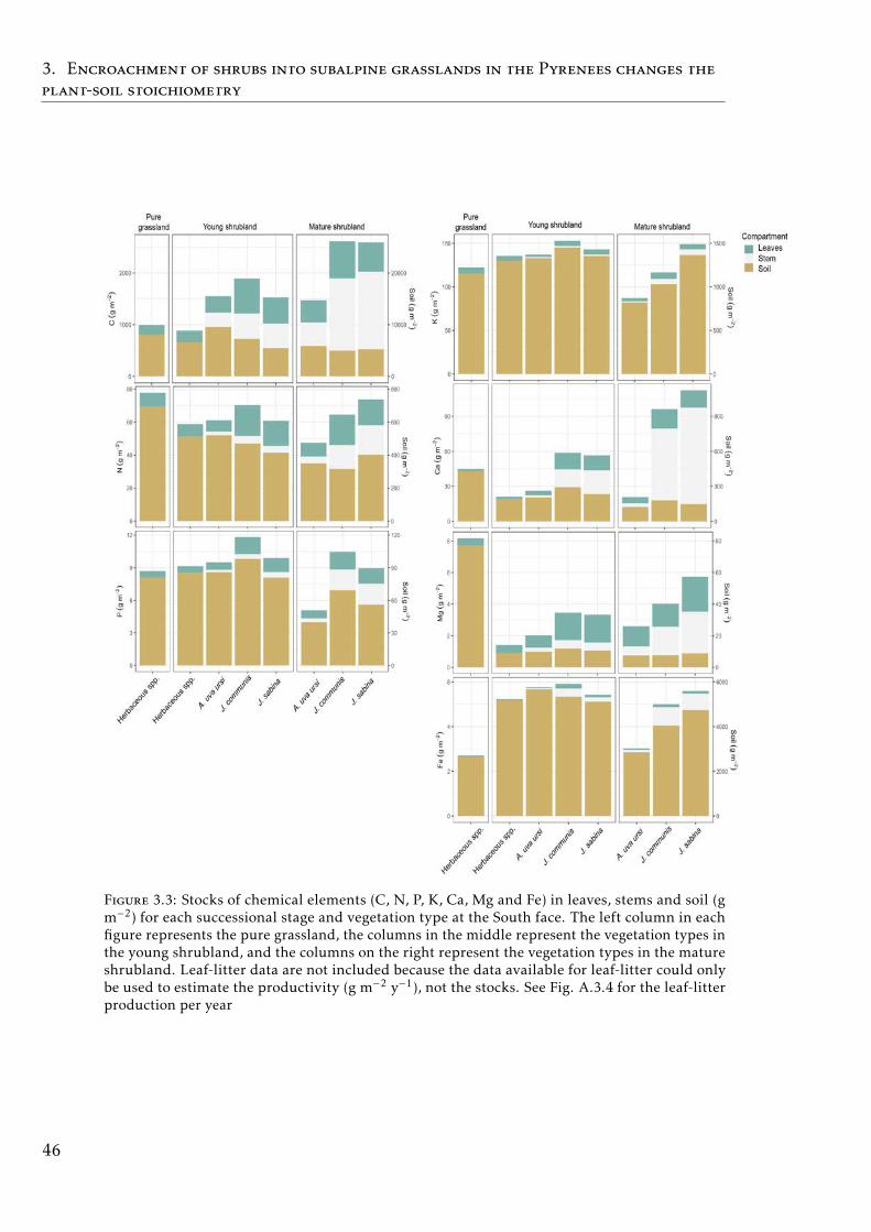
3. Encroachment of shrubs into subalpine grasslands in the Pyrenees changes the
plant-soil stoichiometry
Figure 3.3: Stocks of chemical elements (C, N, P, K, Ca, Mg and Fe) in leaves, stems and soil (gm−2) for each successional stage and vegetation type at the South face. The left column in eachfigure represents the pure grassland, the columns in the middle represent the vegetation types inthe young shrubland, and the columns on the right represent the vegetation types in the matureshrubland. Leaf-litter data are not included because the data available for leaf-litter could onlybe used to estimate the productivity (g m−2 y−1), not the stocks. See Fig. A.3.4 for the leaf-litterproduction per year
46
3.4. Discussion
3.4 Discussion
The plant-soil stoichiometry spectrum differed greatly along the succession frompure grassland to mature shrubland (Fig. 3.1), as initially hypothesised. The shiftin plant-soil stoichiometry spectrum was more apparent and consistent betweenthe pure grassland and the young shrubland than between the young and matureshrubland (Tables 3.1 and 3.3), suggesting that changes in growth forms (fromgrass-dominated to shrub-dominated) play a greater role in shaping the plant-soilstoichiometry spectrum than differences in successional stage as such. In fact, theplant-soil stoichiometry spectrum is expected to be primarily shaped by changesin abiotic and/or biotic factors, such as changes in vegetation along the succession.This is evidenced by the shift between herbaceous spp. and shrubs, from highfoliar [N] and [K] for herbaceous spp. to high foliar [C], [Ca], [Mg], C:N and C:Pratios and low [N], [P] or [K] for shrubs (Table 3.1 and A.3.4); or from low tohigh [C], C:N and C:P ratios in litter, and from high to low [N], [P], [Mg] and[Ca] in soil. Such changes in stoichiometry may have major consequences on thefunctioning of ecosystems (Eldridge et al. 2011). For example, the high [C] andC:N and C:P ratios in the shrub leaves and leaf-litter promote the formation ofrecalcitrant organic matter accumulation with slow decomposition rates in the topsoil of shrubland compared to the grassland (Ninot et al. 2010b; Garcia-Pausas etal. 2017).
The changes in foliar chemical spectrum enabled us to detect shifts in thebiogeochemical niche (Urbina et al. 2017; Penuelas et al. 2019)(Fig. A.3.6). Wefound that shrubs and herbaceous spp. differed significantly in their biogeochem-ical niche, as expected from these two contrasting growth forms. For example,herbaceous spp. in the pure grassland had higher foliar nutrient concentrations(N, K), characteristic of plants with fast growth rates; whereas shrubs had higherC concentration and C:N and C:P ratios in leaves, characteristic of plants withslow growth rates (Agren 2004; Sardans et al. 2012b; Zechmeister-Boltenstern etal. 2015).
The stoichiometry changes in the plant aboveground compartments alongthe succession were coupled with a decrease of the soil concentrations of someessential nutrients needed for plant development. Grau et al. (2019) suggestedthat this decrease in nutrient concentrations in the soil was possibly due to thedecline in nutrient inputs from excrements of domestic herbivores and to thetransfer of nutrients from the soil to the biomass of the shrubs (Horton et al.2009). The allocation of nutrients to the biomass of shrubs could be a mechanismof nutrient accumulation by which shrubs control nutrients in an ecosystemthrough a positive feed-back (Chapin et al. 1997) to outcompete herbaceous spp.and expand into the grassland (Grau et al. 2019). In our study we found thatthe concentrations of N, P and K often decreased in the aboveground biomassalong the succession in both study sites (Tables 3.1 and 3.2); at the same time,the concentrations of soil N, P or K often decreased in the mature shrublandof several shrubs. The stocks of N and P in the aboveground biomass (leaves +stems), though, increased for several shrubs along the succession, particularlyin R. ferrugineum, J. communis and J. sabina (Figs. 3.2 and 3.3). This indicatesthat the dilution of these nutrients in the aboveground biomass of shrubs was
47
3. Encroachment of shrubs into subalpine grasslands in the Pyrenees changes the
plant-soil stoichiometry
overbalanced by their increase in aboveground biomass. This evidences thatshrubs may act as net reservoirs of essential nutrients in the biomass even if theconcentration in the biomass and soil decrease along the succession.
The amount of C and nutrient stocks in aboveground biomass differed notablyamongst shrub species, which implied differences in the final stocks in the matureshrubland within each site. Shrub identity is therefore crucial to understandthe variability in concentrations and stocks of nutrients in the vegetation and inthe soil within each site. However, we also found differences between the Northand South face. Shrubs were generally smaller and less sclerophyllous at Northface (Fig. A.3.5), where solar radiation and evapotranspiration are lower, theslope is smoother, and the soil is deeper than at South face (Ninot et al. 2010a).The increases in the C and nutrient stocks (g m−2) in the aboveground plantcompartments along the succession from grassland to shrubland were less evidentat North face than at South face. In contrast, shrubs developed more woody tissue,were taller and had higher wood density and more sclerophyllous leaves at Southface. This is probably because shrubs are adapted to harsher conditions, with moresolar radiation, higher evapotranspiration, less precipitation, a steeper slope andshallower soil with more rocky outcrops than at North face (Ninot et al. 2010a).
Finally, herbaceous spp. in young shrubland and shrubs in young and matureshrubland showed lower foliar δ15N in leaves and [N] than herbaceous spp. inpure grassland (Fig. A.3.3). This was often coupled with a decrease in soil [N] inthe young and/or mature shrubland for several shrub species (Table 3.1). Theseresults evidence that nitrogen may become limiting in cold ecosystems (Fay et al.2015), such as subalpine ecosystems with high shrub cover (Angulo et al. 2019).Lower δ15N generally indicates more N uptake by ectomycorrhizal or ericoidmycorrhizal fungi compared to arbuscular mycorrhizal plants such as herbaceousspp. (Michelsen et al. 1998), with more recycled N leading to lower N losses fromthe ecosystem (Garten 1993; Robinson 2001; Craine et al. 2009b; Anadon-Rosellet al. 2016). All shrubs at North face are ericaceous and have ericoid mycorrhizae;in the South face, A. uva-ursi hosts both ericoid and ectomycorrhizal fungi. Thus,the lower 15N in young and mature shrubland possibly indicates that more N hadbeen uptake by ericaceous or ectomycorrhizal fungi in a relatively closed N cycle(Angulo et al. 2019). The N uptake by ectomycorrhizal or ericoid mycorrhizalfungi possibly promotes the uptake of organic N (e.g. from litter) by shrubs(Akhmetzhanova et al. 2012) as N becomes more limiting in the soil. This suggeststhat the advance of the succession changed the mechanisms by which plantsuptake N to overcome N limitation.
3.5 Conclusion
Shrub expansion have an important impact in the plant-soil elemental compositionof the grassland ecosystems in the Pyrenes. Grassland ecosystem are dominatedby species with faster nutrients turn-over between the plant-soil compartments,high N, P and K concentrations in the plant aboveground and soil biomass butlimited biomass accumulation capacity. The expansion of shrub, though, favoredthe dominance of long live species, with more conservative strategy, high C:
48

3.5. Conclusion
nutrient ratios and low N, P and K concentration in the aboveground biomass andlow nutrient concentrations in soils. The total stocks of C and nutrients in theaboveground biomass were nevertheless high because the biomass of the matureshrubland was very high compared to the grassland. We thus highlight the roleof shrubs in the sequestration of C and nutrients, through the allocation to theaboveground biomass. Moreover, shrub encroachment alters the strategy withwhich N is acquired, possibly through an increased uptake of N through ericoid orectomycorrhizae. Our results suggested that shrubs play an important role in theC and nutrient sequestration in the aboveground biomass (through the allocationinto the plant compartments) along the succession, where the woody tissuesplay a main role as storage compartment. The changes in plant-soil elementalcomposition and stocks suggest a slowdown of the biogeochemical cycles in thesubalpine mountain areas where shrub encroachment occurred.
49

High foliar K and P resorption efficiencies inold-growth tropical forests growing onnutrient-poor soils 4
51
4. High foliar K and P resorption efficiencies in old-growth tropical forests
growing on nutrient-poor soils
Abstract
Tropical forests in the Guiana Shield store large amounts of aboveground biomass,even though they grow on old, weathered, nutrient-poor soils. Nutrient resorptionfrom leaves before abscission may be very advantageous for trees to avoid nutrientleaching but remains poorly explored in tropical forests. We investigated foliarresorption from the senescent leaves and nutrient stocks in soil, leaves and leaf-litter in two tropical forests in French Guiana, a tropical region with particularlylow total and available phosphorus (P) in the soil. P was the scarcer nutrient storedin the leaves (4.6 and 6.5 kg ha−1), leaf-litter (2.2 and 1.8 kg ham1) and soil (205and 158.7 kg ha−1 in the 0-15 cm layer and 205 and 142 kg ha−1 in the 15-30 cmlayer) in Nouragues and Paracou respectively. Resorption efficiencies were higherfor K and P (total means of 44.6 and 35.9%, respectively) than N (total meanof 10.3%). K resorption was higher in the wet (70.2%) than in the dry (41.7%)season. P resorption was weakly negatively correlated with total soil P but notwith available P, and neither N nor K resorption were correlated with soil N or Kconcentrations. Relationships between nutrient resorption and species functionalcharacteristics (growth rate, wood density, diameter at breast height and specificleaf area) were weak and varied among the nutrients. Phylogenetic relatednessdid not account for the variability in resorption efficiencies. Instead, the level ofnutrient immobilization in foliar compounds probably determine significantly theresorption process. Our results suggest that high K and P resorption efficienciesare an adaptive strategy allowing species to cope with soil nutrient scarcity. Weconclude that nutrient resorption from senescent leaves is a key process for plantsto conserve nutrients in these tropical forests in French Guiana, especially for Kand P, which are difficult to acquire in these old, weathered soils.
• Key words: nutrient, resorption, nitrogen, phosphorus, potassium, recycling,tropical forest, stocks, soil.
4.1 Introduction
Tropical forests store large amounts of aboveground biomass, even though theygrow on old, highly weathered and nutrient-poor soils (Gersmehl 1976; Vitousekand Sanford 1986). This issue has attracted the attention of the ecological com-munity, and several mechanisms have been proposed to explain this apparentparadox (Vitousek and Sanford 1986; Bond 2010; Sayer and Banin 2016; Turneret al. 2018). One proposed essential mechanism is high efficiency of nutrientrecycling on tropical forests growing on nutrient-poor soil. In fact, higher internalnutrient recycling by plants may be a key mechanism to avoid nutrient losses fromaboveground biomass in tropical forests with low soil nutrient concentrations(Vitousek 1984; Brant and Chen 2015; Grau et al. 2017).
The resorption of nutrients from leaves (also called ‘backmigration’, ‘retranslo-cation’, ‘remobilization’ or ‘reabsorption’) is the active withdrawal of nutrientsbefore abscission (Fries 1952; Hill 1980; Killingbeck 1996). This process beginswith senescence, which leads to a series of metabolic changes associated with a de-crease in auxin levels, protein breakdown, chlorophyll degradation and eventually
52
4.1. Introduction
death (Fuente and Leopold 1968). The resorption of foliar nutrients is activatedby kinetin signals, which promote nutrient mobilization through the phloem fromold senescent leaves, as the source, to other plant organs like stems, roots or newleaves, as the sink (Hill 1980). This process of internal nutrient recycling playsan important role in plant nutrition and survival, allowing plants to be moreindependent from external conditions (Aerts 1996; Killingbeck 1996; van Heer-waarden et al. 2002; Reed et al. 2012; Brant and Chen 2015). Nutrient resorptioncan be estimated by resorption efficiency, defined as the percent reduction of anutrient between green and senesced leaves (Killingbeck 2004). The resorptionof nutrients within a plant can vary greatly from year to year depending on theenvironmental conditions, such as soil water availability, timing of abscission andthe amount of shade a plant received (Killingbeck 2004). The capacity of resorp-tion will be firstly determined by the nutrient biochemical limitation, which isthe level of nutrient immobilization in the leaf compounds (compounds of whicheach nutrient is a constituent: enzymes, proteins, DNA, RNA, etc), that will pre-vent mobilization from senescing leaves. Nutrients in structural and recalcitrantcompounds may require high energetic costs to be reabsorbed, and those used forenzymatic machinery for foliar senescence may be unavailable for export fromleaves (Killingbeck 2004).
Highly efficient nutrient cycling in nutrient-poor ecosystems has been postu-lated as a response of species to nutrient-limiting conditions, but the relationshipbetween soil nutrient concentration and nutrient resorption in leaves is not clear(Killingbeck 1996; Aerts and Chapin 2000; Wright and Westoby 2003; Yuan andChen 2009; Brant and Chen 2015). An analysis of global data conducted by Yuanand Chen (2009) reported an increase in the P resorption efficiencies with tem-perature and precipitation, suggesting P resorption efficiency as an indicator of Plimitation in the tropics. Water availability is clearly a major driver of resorption,the reduction in phloem flux transport and water scarcity lead to lower nutrientresorption due the advance of foliar abscission (Killingbeck 2004; Estiarte andPenuelas 2015). Phenology substantially affect resorption because the flower orfruit production will act as a sink strength for the nutrient in senescent leaves(Killingbeck 2004; Estiarte and Penuelas 2015). Phylogenetic relatedness is ex-pected to also play a role in understanding the efficiency of nutrient resorptionamong plant species, with closely related taxa often having similar resorptionefficiencies (Aerts and Van der Piejl 1993; Killingbeck 2004; Sua et al. 2005).
Nitrogen (N), phosphorus (P) and potassium (K) are the most important nutri-ents for plant development (Aerts and Chapin 2000). Nitrogen is the principalconstituent of proteins and nucleic acids in plant cells and is acquired throughthe plant root uptake as nitrate or ammonia present in the soil and return to thesoil through litter inputs, which is why young natural ecosystems are generallypoor in N (Walker and Syers 1976; Turner and Condron 2013). Also, nitrogenfixing species are able to fix atmospheric molecular N (N2) that can be used inthe ecosystem. Nitrogen fixing species are common in all terrestrial ecosystemsand provide large inputs of N to support plant growth (Chapin 1980), whichis important for tropical forests, especially during rapid biomass accumulation(Hedin and Brookshire 2009; Batterman et al. 2013a). Phosphorus is present inplant tissue mainly in energetic forms (ATP and NADPH) and in nucleic acids and
53
4. High foliar K and P resorption efficiencies in old-growth tropical forests
growing on nutrient-poor soils
is provided almost completely by apatite-bearing rocks in the parental material(Chapin 1980). Old-growth tropical forests located on geologically ancient soilsare generally described as P-limited ecosystems (Bruijnzeel 1991; Vitousek et al.2010), because of their limited P availability and total P, low cation exchangecapacity and typically high concentrations of ferric sesquioxides. These occludethe little P that is left in the soil system, making it inaccessible to most organisms,a process that is known as ‘terminal steady state’ (Walker and Syers 1976). Thedeposition of atmospheric dust, however, may represent an important P inputin some tropical forests (Gross et al. 2016). Typically, N is not considered to belimiting in these tropical forests (Walker and Syers 1976; Vitousek and Sanford1986; Tanner et al. 1998), thus we expect that P resorption will be more efficientthan N in old-growth tropical forests.
Potassium represents the most abundant cation (K+) in plant cells and playsa central role in water economy, photosynthetic capacity and nutrient transportin plants, and is thus essential for plant development (Aerts and Chapin 2000;Sardans and Penuelas 2015a). Despite their importance in plant performance, Kresorption efficiencies have been poorly studied (but see Ławniczak 2011; Vergutzet al. 2012). Potassium is highly mobile in plant tissues and is almost completelyprovided by the weathering of soil parental material. Old tropical soils, especiallythose of the Precambrian shield, contain little available K, as described for P, dueto the weathering and leaching of soil over a very long time (Rosolem et al. 2010;Sayer and Banin 2016). Potassium has been described as a co-limiting nutrientfor tree growth in wet lowland tropical forests in Costa Rica (Baribault et al.2012) and the addition of both K and N increased sapling growth in a long-termfertilization experiment in Panama (Wright et al. 2011). We may thus expect thatK will be highly reabsorbed in tropical forests, as expected for P, because theiravailabilities are similarly low in old tropical soils (Rosolem et al. 2010; Wright etal. 2011). Resorption efficiency in trees is generally higher for P than N (Yuan andChen 2009; Vergutz et al. 2012), but very few studies have reported K resorptionefficiencies (but see Ławniczak 2011; Vergutz et al. 2012).
In this study, we explored the stocks (C, N, P and K) and the resorption efficien-cies (N, P and K) of essential elements in aboveground (leaves and leaf-litter) andsoil compartments in two old-growth tropical forests growing on old, nutrient-poor soils. We first calculated the stocks (kg ha−1) of carbon (C) and nutrients(N, P and K) of tree leaves, leaf-litter at the soil surface, and soil at two depths(0-15 and 15-30 cm). We then calculated the efficiencies of nutrient (N, P andK) resorption for 39 tropical tree species in the dry season and for a subset of 18species in the wet and dry seasons to determine if soil nutrient concentration andseasonality affected nutrient resorption. We investigated the possible relationshipsbetween the nutrient resorption and some functional characteristics: growth rate,wood density, diameter at breast height (DBH) and specific leaf area (SLA). Wealso investigated the possible variability in the nutrient resorption efficiencies dueto the phylogeny. We calculated the phylogenetic signals of the species (Pagel’s λand Blomberg’s K) to determine whether closely related species tended to havemore similar resorption efficiencies than distantly related species.
We hypothesized that: 1) nutrients that has been lost greatly by soil leachingwould be stored in larger quantities (kg ha−1) in the aboveground biomass (leaves
54
4.2. Material & Methods
and leaf-litter) than in the soil, whereas soil would store larger quantities of Cand N than the aboveground biomass; 2) K and P would have higher resorptionefficiencies than N, because they are less available in the soil and more mobile inthe plant; 3) nutrient resorption efficiencies would be higher in the wet than thedry season, because water conductance and the capacity to transport nutrientswould be higher in the wet season; 4) species with slow growth rates and highwood densities (a more conservative strategy) would reabsorb more nutrientsthan species with high growth rates and low wood densities (a more acquisitionstrategy), which would probably depend more on the nutrients in the litter andsoil; and 5) resorption efficiencies would be more similar among closely thandistantly related species.
4.2 Material & Methods
Study area
The study was conducted in French Guiana, a tropical region in the north-eastern part of South America. French Guiana is almost completely covered bytropical forest and has an old, nutrient-poor Precambrian substrate, characteristicof the Guiana Shield formation (Bongers et al. 2001; Epron et al. 2006; Courtois etal. 2018). Two study sites were selected: Paracou (5°18N, 52°53W) and Nouragues(4°05’N, 52°41’W) (Fig. A.4.1a). Paracou is located in Sinnamary, 15 km inlandfrom the coast, in an undisturbed forested area characterized by smooth mosaichills (Janssens et al. 1998; Epron et al. 2006). The Nouragues Research Station issituated in the center of the country, which is covered by extensive primary forestwith granitic hills (Bongers et al. 2001). The climate at both sites is typical oftropical rainforests, with two marked seasons: a rainy season from December toJuly and a dry season from August to November. Mean annual rainfall is similar inboth study sites (2990 and 3041 mm y−1 at Nouragues and Paracou, respectively)(Bongers et al. 2001; Aguilos et al. 2018). The soils at both sites are classified asOxisols in the USDA soil classification, typically strongly weathered nutrient-poorred or yellow soils from old, stable geomorphic surfaces rich in sesquioxides (IUSSWorking Group 2014).
Experimental design
Two field campaigns were carried out in 2015, from May to the end of June inthe rainy season and from the beginning of October until late November in thedry season. Twelve experimental plots were established at each site to representthe spatial variability, including the top of the hills (top plots), the slope of thehills (slope plots) and the bottom of the hills next to rivulets (bottom plots) (Fig.A.4.1b). We established four plots of 50 × 50 m (20-100 m the between plots) ateach topographic position and an inner 20 × 20 m sampling area in each plot. Wemarked, tagged and identified all trees in each plot (50 × 50 m) and measured theDBH of all trees with DBHs >10 cm.
55
4. High foliar K and P resorption efficiencies in old-growth tropical forests
growing on nutrient-poor soils
We established five sampling points within each plot, one in the center andone in each corner of the square, to collect leaf-litter at the soil surface and thesoil samples (Fig. A.4.1c). We collected all mixed leaf-litter at the soil surface(leaf-litter hereafter) in an area of 20 × 20 cm at these 5 sampling points withineach plot. These samples where oven-dried at 70 °C to constant weights. Soilsamples were collected in each sampling points with a soil auger 4 cm in diameterfrom two layers (0-15 and 15-30 cm) and sieved through a 2 mm sieve. Soil weightwas then determined after drying at 105°C for 24 h and divided by the corervolume to obtain the soil bulk density.
In each plot, we collected leaves from three canopy emergent trees and twosubcanopy trees in the sampling areas based on their DBH, trying to maximize thenumber of species sampled (if two trees belonged to the same species, we chose thenext tree of a different species but with similar size). Green leaves were collected(between 5 or 10 leaves by tree depending of the leaf size) by tree climbers fromthe upper, mostly sunlit leaves and lower, mainly shaded leaves of the canopy toobtain two contrasting canopy conditions. The leaves were immediately frozenin liquid N. If the climbers could not reach trees in the sampling areas, then wechose trees in the buffer zones (between the inner 20 × 20 m square and the outer50 × 50 m areas) following the same criteria.
Tree climbers also collected senescent leaves when still attached to the tree andcould be easily collected by shaking the branch. Taking both study sites together,we were able to collect senescent leaves from a total of 39 species during the dryseason (Appendix 4, Table A.4.1). A subset of 18 species from the 39 collected indry season were collected also in the wet season (Table A.4.2).
Chemical analysis
Samples were freeze-dried (Christ Freeze Dryer ALPHA 1-2 LDplus. Osterodeam Harz, Germany), ground with a ball mill (Retsch, model MM400. RestchGmbH, Haan Germany), and weighed with an AB204 Mettler Toledo (MettlerToledo, Barcelona, Spain) balance. Leaf C and N (dry weight (dw) of nutrient/dwof sample × 100) were determined by gas chromatography. The amount of sampleused was based on % C and % N in each type of sample. For the leaves, senescentleaves and the leaf-litter, 4.5 mg of pulverized dry sample were weighed andsealed in tin capsules. For the soil samples, 9 mg for the 0-15 cm layer (sampleswith high organic-matter content) and 11 mg for the 15-30 cm layer (samples withmoderate-low organic-matter content) were used. Leaves, senescent leaves andleaf-litter samples were then analyzed with a PDZ Europa ANCA-GSL elementalanalyzer interfaced to a PDZ Europa 20-20 isotope ratio mass spectrometer (SerconLtd. Cheshire, UK), and soils samples with an Elementar Vario EL Cube or MicroCube elemental analyzer (Elementar Analysensysteme GmbH. Hanau, Germany).The samples were combusted at 1000°C (plant material) in a reactor packed withchromium oxide and silvered copper oxide and at 1080 °C (soils) in a reactorpacked with copper oxide and tungsten (VI) oxide. Oxides were then removed in areduction reactor (reduced copper at 650 °C). The samples were interspersed withseveral replicates of at least two laboratory standards during the analysis. Theselaboratory standards, selected to be compositionally similar to the samples being
56
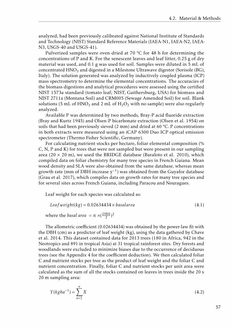
4.2. Material & Methods
analyzed, had been previously calibrated against National Institute of Standardsand Technology (NIST) Standard Reference Materials (IAEA-N1, IAEA-N2, IAEA-N3, USGS-40 and USGS-41).
Pulverized samples were oven-dried at 70 °C for 48 h for determining theconcentrations of P and K. For the senescent leaves and leaf litter, 0.25 g of drymaterial was used, and 0.1 g was used for soil. Samples were diluted in 5 mL ofconcentrated HNO3 and digested in a Milestone Ultrawave digestor (Sorisole (BG),Italy). The solution generated was analyzed by inductively coupled plasma (ICP)mass spectrometry to determine the elemental concentrations. The accuracies ofthe biomass digestions and analytical procedures were assessed using the certifiedNIST 1573a standard (tomato leaf; NIST, Gaithersburg, USA) for biomass andNIST 2711a (Montana Soil) and CRM005 (Sewage Amended Soil) for soil. Blanksolutions (5 mL of HNO3 and 2 mL of H2O2 with no sample) were also regularlyanalyzed.
Available P was determined by two methods, Bray-P acid fluoride extraction(Bray and Kurtz 1945) and Olsen-P bicarbonate extraction (Olsen et al. 1954) onsoils that had been previously sieved (2 mm) and dried at 60 °C. P concentrationsin both extracts were measured using an iCAP 6300 Duo ICP optical emissionspectrometer (Thermo Fisher Scientific, Germany).
For calculating nutrient stocks per hectare, foliar elemental composition (%C, N, P and K) for trees that were not sampled but were present in our samplingarea (20 × 20 m), we used the BRIDGE database (Baraloto et al. 2010), whichcompiled data on foliar chemistry for many tree species in French Guiana. Meanwood density and SLA were also obtained from the same database, whereas meangrowth rate (mm of DBH increase y−1) was obtained from the Guyafor database(Grau et al. 2017), which compiles data on growth rates for many tree species andfor several sites across French Guiana, including Paracou and Nouragues.
Leaf weight for each species was calculated as:
Leaf weight(kg) = 0.02634434× basalarea (4.1)
where the basal area = π ×(DBH2 )2
The allometric coefficient (0.02634434) was obtained by the power-law fit withthe DBH (cm) as a predictor of leaf weight (kg), using the data gathered by Chaveet al. 2014. This dataset contained data for 2013 trees (180 in Africa, 942 in theNeotropics and 891 in tropical Asia) at 31 tropical rainforest sites. Dry forests andwoodlands were excluded to minimize biases due to the occurrence of deciduoustrees (see the Appendix 4 for the coefficient deduction). We then calculated foliarC and nutrient stocks per tree as the product of leaf weight and the foliar C andnutrient concentration. Finally, foliar C and nutrient stocks per unit area werecalculated as the sum of all the stocks contained on leaves in trees inside the 20 x20 m sampling area:
Y (kgha−1) =n∑n=1
X (4.2)
57
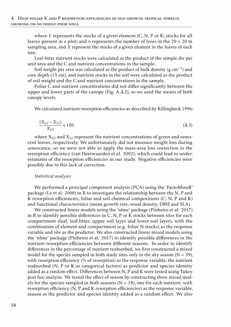
4. High foliar K and P resorption efficiencies in old-growth tropical forests
growing on nutrient-poor soils
where Y represents the stocks of a given element (C, N, P or K; stocks for allleaves present in a plot) and n represents the number of trees in the 20 × 20 msampling area, and X represent the stocks of a given element in the leaves of eachtree.
Leaf-litter nutrient stocks were calculated as the product of the sample dw perunit area and the C and nutrient concentrations in the sample.
Soil weight per area was calculated as the product of bulk density (g cm−3) andcore depth (15 cm), and nutrient stocks in the soil were calculated as the productof soil weight and the C and nutrient concentrations in the sample.
Foliar C and nutrient concentrations did not differ significantly between theupper and lower parts of the canopy (Fig. A.4.2), so we used the means of bothcanopy levels.
We calculated nutrient-resorption efficiencies as described by Killingbeck 1996:
(XGl −XS l)XGl
× 100 (4.3)
where XGl and XS l represent the nutrient concentrations of green and senes-cent leaves, respectively. We unfortunately did not measure weight loss duringsenescence, so we were not able to apply the mass-area loss correction to theresorption efficiency (van Heerwaarden et al. 2002), which could lead to under-estimates of the resorption efficiencies in our study. Negative efficiencies werepossibly due to this lack of correction.
Statistical analyses
We performed a principal component analysis (PCA) using the ‘FactoMineR’package (Le et al. 2008) in R to investigate the relationship between the N, P andK resorption efficiencies, foliar and soil chemical compositions (C, N, P and K)and functional characteristics (mean growth rate, wood density, DBH and SLA).
We constructed linear models using the ‘nlme’ package (Pinheiro et al. 2017)in R to identify possible differences in C, N, P or K stocks between sites for eachcompartment (leaf, leaf-litter, upper soil layer and lower soil layer), with thecombination of element and compartment (e.g. foliar N stocks) as the responsevariable and site as the predictor. We also constructed linear mixed models usingthe ‘nlme’ package (Pinheiro et al. 2017) to identify possible differences in thenutrient resorption efficiencies between different seasons. In order to identifydifferences in the percentage of nutrient reabsorbed, we first constructed a mixedmodel for the species sampled in both study sites only in the dry season (N = 39),with resorption efficiency (% of resorption) as the response variable, the nutrientreabsorbed (N, P or K as categorical factors) as predictor and species identityadded as a random effect. Differences between N, P and K were tested using Tukeypost hoc analysis. We tested the effect of season by constructing three mixed mod-els for the species sampled in both seasons (N = 18), one for each nutrient, withresorption efficiency (N, P and K resorption efficiencies) as the response variable,season as the predictor and species identity added as a random effect. We also
58
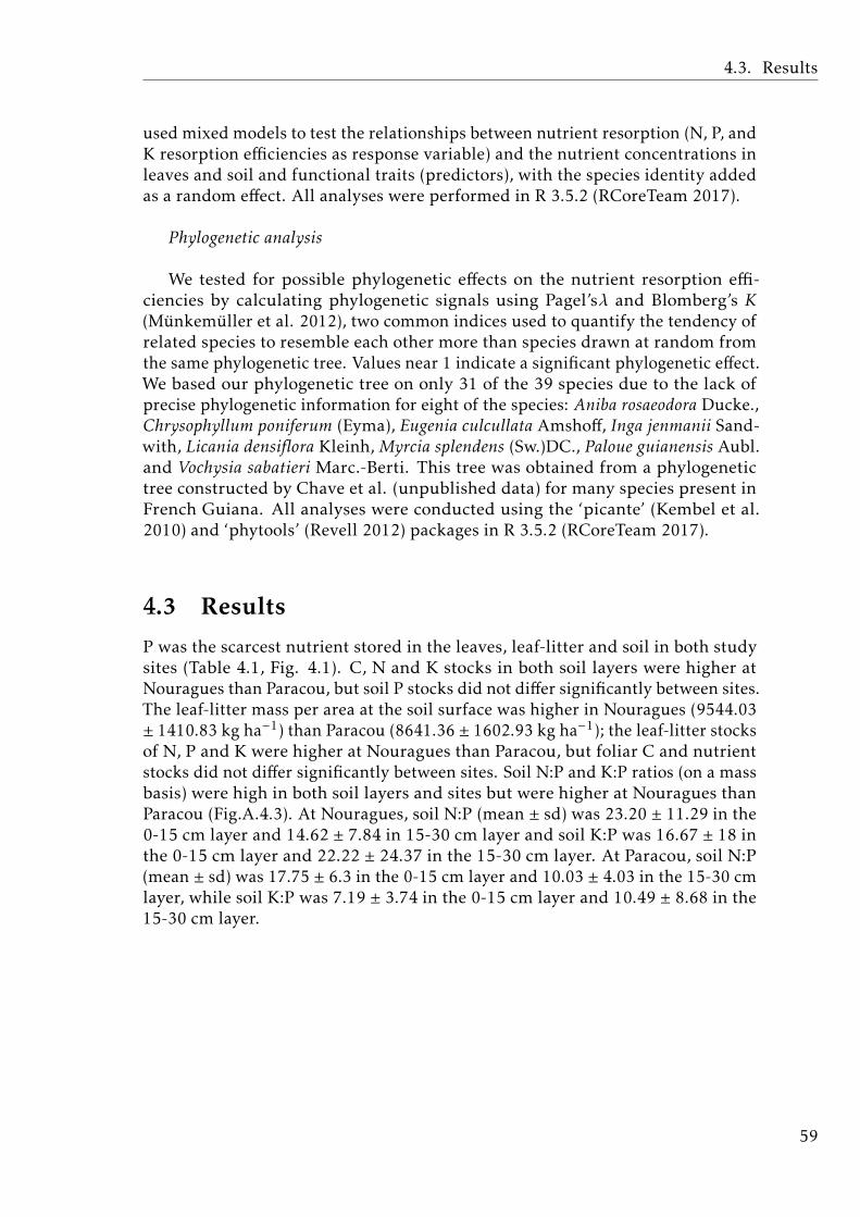
4.3. Results
used mixed models to test the relationships between nutrient resorption (N, P, andK resorption efficiencies as response variable) and the nutrient concentrations inleaves and soil and functional traits (predictors), with the species identity addedas a random effect. All analyses were performed in R 3.5.2 (RCoreTeam 2017).
Phylogenetic analysis
We tested for possible phylogenetic effects on the nutrient resorption effi-ciencies by calculating phylogenetic signals using Pagel’sλ and Blomberg’s K(Munkemuller et al. 2012), two common indices used to quantify the tendency ofrelated species to resemble each other more than species drawn at random fromthe same phylogenetic tree. Values near 1 indicate a significant phylogenetic effect.We based our phylogenetic tree on only 31 of the 39 species due to the lack ofprecise phylogenetic information for eight of the species: Aniba rosaeodora Ducke.,Chrysophyllum poniferum (Eyma), Eugenia culcullata Amshoff, Inga jenmanii Sand-with, Licania densiflora Kleinh, Myrcia splendens (Sw.)DC., Paloue guianensis Aubl.and Vochysia sabatieri Marc.-Berti. This tree was obtained from a phylogenetictree constructed by Chave et al. (unpublished data) for many species present inFrench Guiana. All analyses were conducted using the ‘picante’ (Kembel et al.2010) and ‘phytools’ (Revell 2012) packages in R 3.5.2 (RCoreTeam 2017).
4.3 Results
P was the scarcest nutrient stored in the leaves, leaf-litter and soil in both studysites (Table 4.1, Fig. 4.1). C, N and K stocks in both soil layers were higher atNouragues than Paracou, but soil P stocks did not differ significantly between sites.The leaf-litter mass per area at the soil surface was higher in Nouragues (9544.03± 1410.83 kg ha−1) than Paracou (8641.36 ± 1602.93 kg ha−1); the leaf-litter stocksof N, P and K were higher at Nouragues than Paracou, but foliar C and nutrientstocks did not differ significantly between sites. Soil N:P and K:P ratios (on a massbasis) were high in both soil layers and sites but were higher at Nouragues thanParacou (Fig.A.4.3). At Nouragues, soil N:P (mean ± sd) was 23.20 ± 11.29 in the0-15 cm layer and 14.62 ± 7.84 in 15-30 cm layer and soil K:P was 16.67 ± 18 inthe 0-15 cm layer and 22.22 ± 24.37 in the 15-30 cm layer. At Paracou, soil N:P(mean ± sd) was 17.75 ± 6.3 in the 0-15 cm layer and 10.03 ± 4.03 in the 15-30 cmlayer, while soil K:P was 7.19 ± 3.74 in the 0-15 cm layer and 10.49 ± 8.68 in the15-30 cm layer.
59
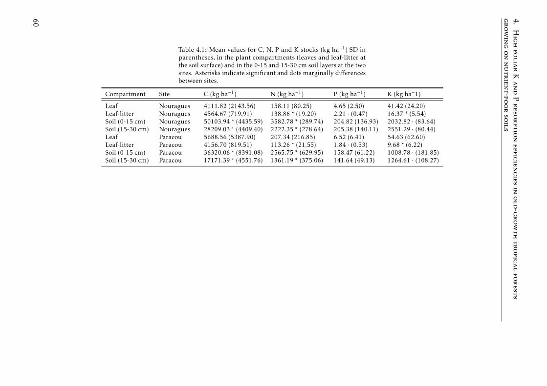
4.HighfoliarKandPresorptionefficienciesinold-growthtropicalforests
growingonnutrient-poorsoils
Table 4.1: Mean values for C, N, P and K stocks (kg ha−1) SD inparentheses, in the plant compartments (leaves and leaf-litter atthe soil surface) and in the 0-15 and 15-30 cm soil layers at the twosites. Asterisks indicate significant and dots marginally differencesbetween sites.
Compartment Site C (kg ha−1) N (kg ha−1) P (kg ha−1) K (kg ha−1)
Leaf Nouragues 4111.82 (2143.56) 158.11 (80.25) 4.65 (2.50) 41.42 (24.20)Leaf-litter Nouragues 4564.67 (719.91) 138.86 * (19.20) 2.21 · (0.47) 16.37 * (5.54)Soil (0-15 cm) Nouragues 50103.94 * (4435.59) 3582.78 * (289.74) 204.82 (136.93) 2032.82 · (83.64)Soil (15-30 cm) Nouragues 28209.03 * (4409.40) 2222.35 * (278.64) 205.38 (140.11) 2551.29 · (80.44)Leaf Paracou 5688.56 (5387.90) 207.34 (216.85) 6.52 (6.41) 54.63 (62.60)Leaf-litter Paracou 4156.70 (819.51) 113.26 * (21.55) 1.84 · (0.53) 9.68 * (6.22)Soil (0-15 cm) Paracou 36320.06 * (8391.08) 2565.75 * (629.95) 158.47 (61.22) 1008.78 · (181.85)Soil (15-30 cm) Paracou 17171.39 * (4551.76) 1361.19 * (375.06) 141.64 (49.13) 1264.61 · (108.27)
60
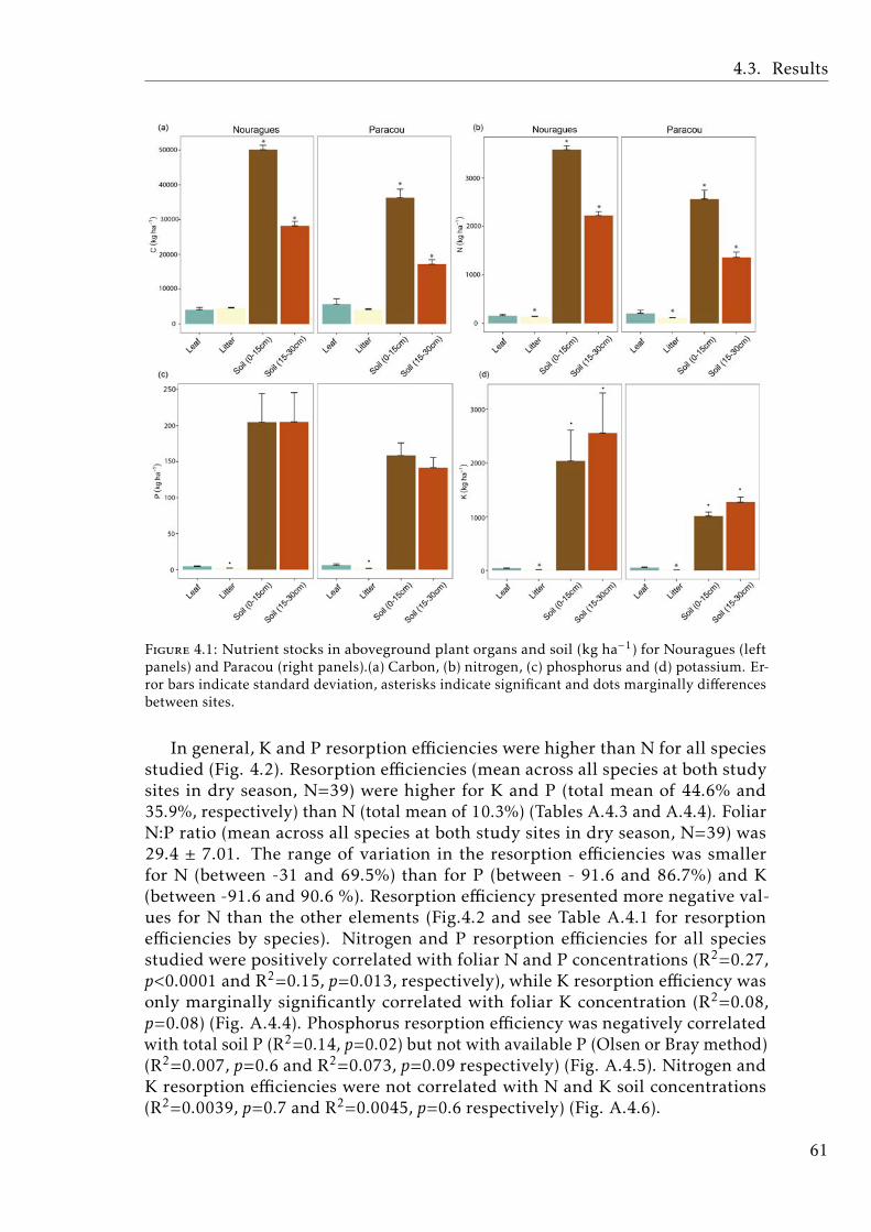
4.3. Results
Figure 4.1: Nutrient stocks in aboveground plant organs and soil (kg ha−1) for Nouragues (leftpanels) and Paracou (right panels).(a) Carbon, (b) nitrogen, (c) phosphorus and (d) potassium. Er-ror bars indicate standard deviation, asterisks indicate significant and dots marginally differencesbetween sites.
In general, K and P resorption efficiencies were higher than N for all speciesstudied (Fig. 4.2). Resorption efficiencies (mean across all species at both studysites in dry season, N=39) were higher for K and P (total mean of 44.6% and35.9%, respectively) than N (total mean of 10.3%) (Tables A.4.3 and A.4.4). FoliarN:P ratio (mean across all species at both study sites in dry season, N=39) was29.4 ± 7.01. The range of variation in the resorption efficiencies was smallerfor N (between -31 and 69.5%) than for P (between - 91.6 and 86.7%) and K(between -91.6 and 90.6 %). Resorption efficiency presented more negative val-ues for N than the other elements (Fig.4.2 and see Table A.4.1 for resorptionefficiencies by species). Nitrogen and P resorption efficiencies for all speciesstudied were positively correlated with foliar N and P concentrations (R2=0.27,p<0.0001 and R2=0.15, p=0.013, respectively), while K resorption efficiency wasonly marginally significantly correlated with foliar K concentration (R2=0.08,p=0.08) (Fig. A.4.4). Phosphorus resorption efficiency was negatively correlatedwith total soil P (R2=0.14, p=0.02) but not with available P (Olsen or Bray method)(R2=0.007, p=0.6 and R2=0.073, p=0.09 respectively) (Fig. A.4.5). Nitrogen andK resorption efficiencies were not correlated with N and K soil concentrations(R2=0.0039, p=0.7 and R2=0.0045, p=0.6 respectively) (Fig. A.4.6).
61
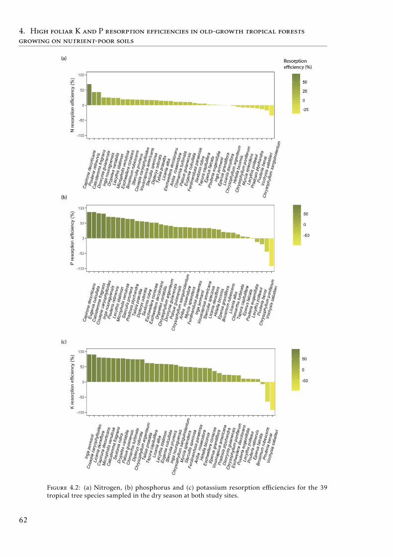
4. High foliar K and P resorption efficiencies in old-growth tropical forests
growing on nutrient-poor soils
Figure 4.2: (a) Nitrogen, (b) phosphorus and (c) potassium resorption efficiencies for the 39tropical tree species sampled in the dry season at both study sites.
62
4.3. Results
Potassium, P and N resorptions tended to be higher in the wet than in the dryseason for all the species (Fig. 4.3). K resorption was significantly higher in thewet (70.19 % ± 18.7) than the dry season (41.7 % ± 25.26) when all the specieswere averaged (total mean across all the species for each season, N=18), whereasN and P resorption efficiencies did not differ significantly between seasons (TableA.4.5, see Table A.4.2 for resorption efficiencies by species in each season).
The PCA indicated that foliar C, N and P concentrations were uncoupled fromsoil C, N and P concentrations. Foliar K was coupled positively with soil K andmean growth rate but negatively with soil C, N and P (Fig. 4.4). N and P resorp-tion efficiencies were positively coupled with their foliar concentrations, but Kresorption was not. The relationships between nutrient resorption efficienciesand functional characteristics of the species were usually weak but statisticallysignificant (Fig. A.4.7). Phosphorus and K resorption efficiencies were slightlynegatively correlated with wood density (R2=0.16, p=0.026 and R2=0.12, p=0.052,respectively), N resorption efficiency was negatively correlated with mean DBH(R2=0.14, p=0.037) and P resorption efficiency was marginally positively cor-related with SLA (R2=0.13, p=0.096) (Fig. A.4.7). Mean growth rate was notsignificantly correlated with nutrient resorption. Mean and sd values for nutri-ent concentrations in leaves and senescent leaves for the all the species studiedare summarized in the Table A.4.6 and mean and sd values for soil elementconcentration in the Table A.4.7.
Pagel’s λ and Blomberg’s K indices showed no significant differences in theresorption efficiencies in relation to the phylogenetic distances between species.Thus, resorption efficiencies were not more similar between closely than distantlyrelated species (Table A.4.8 and see Fig A.4.8 for the phylogenetic tree).
63
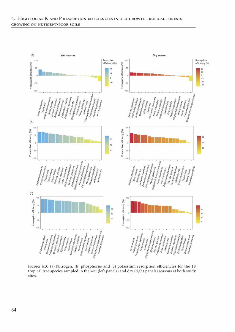
4. High foliar K and P resorption efficiencies in old-growth tropical forests
growing on nutrient-poor soils
Figure 4.3: (a) Nitrogen, (b) phosphorus and (c) potassium resorption efficiencies for the 18tropical tree species sampled in the wet (left panels) and dry (right panels) seasons at both studysites.
64
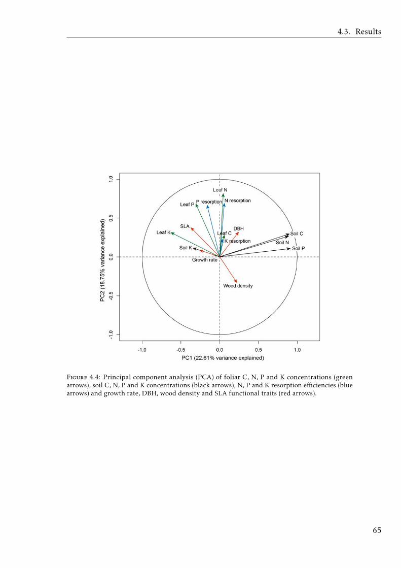
4.3. Results
Figure 4.4: Principal component analysis (PCA) of foliar C, N, P and K concentrations (greenarrows), soil C, N, P and K concentrations (black arrows), N, P and K resorption efficiencies (bluearrows) and growth rate, DBH, wood density and SLA functional traits (red arrows).
65
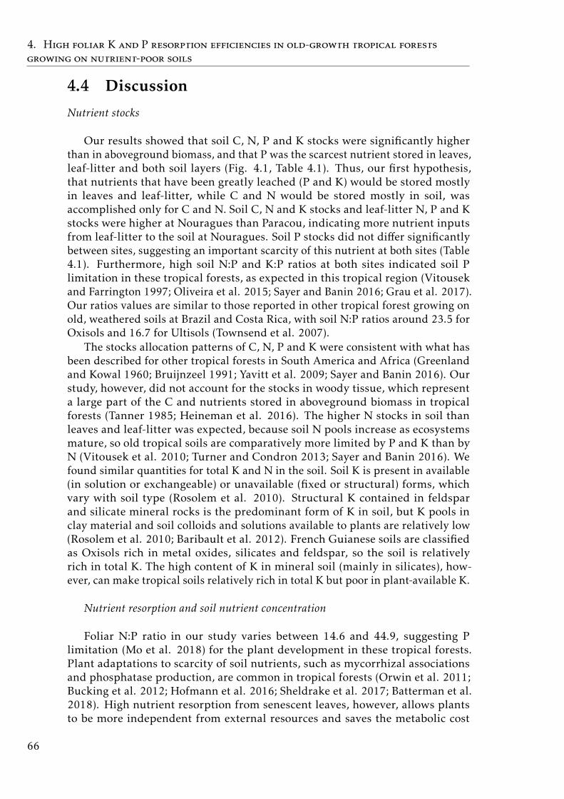
4. High foliar K and P resorption efficiencies in old-growth tropical forests
growing on nutrient-poor soils
4.4 Discussion
Nutrient stocks
Our results showed that soil C, N, P and K stocks were significantly higherthan in aboveground biomass, and that P was the scarcest nutrient stored in leaves,leaf-litter and both soil layers (Fig. 4.1, Table 4.1). Thus, our first hypothesis,that nutrients that have been greatly leached (P and K) would be stored mostlyin leaves and leaf-litter, while C and N would be stored mostly in soil, wasaccomplished only for C and N. Soil C, N and K stocks and leaf-litter N, P and Kstocks were higher at Nouragues than Paracou, indicating more nutrient inputsfrom leaf-litter to the soil at Nouragues. Soil P stocks did not differ significantlybetween sites, suggesting an important scarcity of this nutrient at both sites (Table4.1). Furthermore, high soil N:P and K:P ratios at both sites indicated soil Plimitation in these tropical forests, as expected in this tropical region (Vitousekand Farrington 1997; Oliveira et al. 2015; Sayer and Banin 2016; Grau et al. 2017).Our ratios values are similar to those reported in other tropical forest growing onold, weathered soils at Brazil and Costa Rica, with soil N:P ratios around 23.5 forOxisols and 16.7 for Ultisols (Townsend et al. 2007).
The stocks allocation patterns of C, N, P and K were consistent with what hasbeen described for other tropical forests in South America and Africa (Greenlandand Kowal 1960; Bruijnzeel 1991; Yavitt et al. 2009; Sayer and Banin 2016). Ourstudy, however, did not account for the stocks in woody tissue, which representa large part of the C and nutrients stored in aboveground biomass in tropicalforests (Tanner 1985; Heineman et al. 2016). The higher N stocks in soil thanleaves and leaf-litter was expected, because soil N pools increase as ecosystemsmature, so old tropical soils are comparatively more limited by P and K than byN (Vitousek et al. 2010; Turner and Condron 2013; Sayer and Banin 2016). Wefound similar quantities for total K and N in the soil. Soil K is present in available(in solution or exchangeable) or unavailable (fixed or structural) forms, whichvary with soil type (Rosolem et al. 2010). Structural K contained in feldsparand silicate mineral rocks is the predominant form of K in soil, but K pools inclay material and soil colloids and solutions available to plants are relatively low(Rosolem et al. 2010; Baribault et al. 2012). French Guianese soils are classifiedas Oxisols rich in metal oxides, silicates and feldspar, so the soil is relativelyrich in total K. The high content of K in mineral soil (mainly in silicates), how-ever, can make tropical soils relatively rich in total K but poor in plant-available K.
Nutrient resorption and soil nutrient concentration
Foliar N:P ratio in our study varies between 14.6 and 44.9, suggesting Plimitation (Mo et al. 2018) for the plant development in these tropical forests.Plant adaptations to scarcity of soil nutrients, such as mycorrhizal associationsand phosphatase production, are common in tropical forests (Orwin et al. 2011;Bucking et al. 2012; Hofmann et al. 2016; Sheldrake et al. 2017; Batterman et al.2018). High nutrient resorption from senescent leaves, however, allows plantsto be more independent from external resources and saves the metabolic cost
66
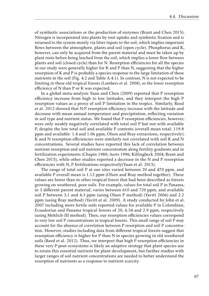
4.4. Discussion
of symbiotic associations or the production of enzymes (Brant and Chen 2015).Nitrogen is incorporated into plants by root uptake and symbiotic fixation and isreturned to the system mostly via litter inputs to the soil, which implies importantflows between the atmosphere, plants and soil (open cycle). Phosphorus and K,however, can only be acquired from the parent material and must be taken up byplant roots before being leached from the soil, which implies a lower flow betweenplants and soil (closed cycle) than for N. Resorption efficiencies for all the speciesin our study were generally higher for K and P than N, suggesting that the higherresorption of K and P is probably a species response to the large limitation of thesenutrients in the soil (Fig. 4.2 and Table A.4.1). In contrast, N is not expected to belimiting in these old tropical forests (Lambers et al. 2008), so the lower resorptionefficiency of N than P or K was expected.
In a global meta-analysis Yuan and Chen (2009) reported that P resorptionefficiency increase from high to low latitudes, and they interpret the high Presorption values as a proxy of soil P limitation in the tropics. Similarly, Reedet al. 2012 showed that N:P resorption efficiency increase with the latitude anddecrease with mean annual temperature and precipitation, reflecting variationin soil type and nutrient status. We found that P resorption efficiencies, however,were only weakly negatively correlated with total soil P but not with availableP, despite the low total soil and available P contents (overall mean total: 119.8ppm and available: 1.4 and 1.06 ppm, Olsen and Bray extractions, respectively).K and N resorption efficiencies were similarly not correlated with soil K and Nconcentrations. Several studies have reported this lack of correlation betweennutrient resorption and soil nutrient concentration along fertility gradients and infertilization experiments (Chapin 1980; Aerts 1996; Killingbeck 2004; Brant andChen 2015), while other studies reported a decrease in the N and P resorptionefficiencies with N, P fertilizations respectively(Yuan et al. 2015).
The range of total soil P at our sites varied between 20 and 470 ppm, andavailable P overall mean is 1.12 ppm (Olsen and Bray method together). Thesevalues are lower than in other tropical forest that had been described as forestsgrowing on weathered, poor soils. For example, values for total soil P in Panama,in 3 different parent material, varies between 610 and 720 ppm, and availablesoil P between 3.1 and 4.3 ppm (using Olsen P method) (Yavitt 2006) and 2.2ppm (using Bray method) (Yavitt et al. 2009). A study conducted by John et al.2007 including more fertile soils reported values for available P in Colombian,Ecuadorian and Panama tropical forests of 20, 6.34 and 2.9 ppm, respectively(using Mehlich-III method). Then, our resorption efficiencies values correspondto very low soil P concentrations in tropical forests. This small range of soil P mayaccount for the absence of correlation between P resorption and soil P concentra-tion. However, studies including data from different tropical forests suggest thatresorption efficiency is higher for P than N in species growing in old weatheredsoils (Reed et al. 2012). Thus, we interpret that high P resorption efficiencies inthese very P-poor ecosystems is likely an adaptive strategy that plant species useto retain this essential nutrient for plant development, but further studies withlarger ranges of soil nutrient concentrations are needed to better understand theresorption of nutrients as a response to nutrient scarcity.
67
4. High foliar K and P resorption efficiencies in old-growth tropical forests
growing on nutrient-poor soils
Nutrient resorption and biochemical limitation
The order of average nutrient resorption efficiencies for all species (K ≥ P >N) was opposite to the immobilization of each of these nutrients in plant tissues(N > P > K). The level of immobilization of nutrients in foliar tissue will largelydetermine the capacity of nutrient recovery from senescent leaves (Killingbeck2004; Kobe et al. 2005). N is highly immobilized in plants e.g. in proteins,enzymes and nucleic acids (Chapin 1980; Sua et al. 2005), P is immobilizedmainly in energetic forms (less than N but more than K) (Walker and Syers 1976;Condron et al. 2013) and K is a free cation in plant cells (Sardans and Penuelas2015a). Nutrients more involved in the enzymatic metabolism of foliar senescence,such as N, or energetic forms necessary to export nutrients from leaves, such as P,will be partially unavailable for resorption (Killingbeck 2004). K and P may thusbe reabsorbed more easily than N, matching the pattern we found. Resorptionefficiency was more variable for P and K than N, and N resorption efficiencypresent more negative values. Aerts and Chapin (2000) previously reported thisdifference in the variation of P and N resorption efficiencies for different growthforms of plants, but the explanation of this difference was not addressed. Perhaps,the higher immobilization of N than P in leaves compounds probably accountsfor the variability of N resorption efficiency. Additionally, Han et al. (2013) alsoreported higher variability in the P resorption efficiency than N in a global dataset.They relate this variability with the comparably greater importance of P resorptionfor plant nutrient conservation than N.
Furthermore, we found that N and P resorption showed a positive correlationwith their concentration in leaves, while K was only marginally correlated. Thisis contrary with what has been reported in global meta-analyses, where nutrientresorption efficiency decrease with the increase in leaf nutrient status (Kobe et al.2005; Vergutz et al. 2012). Our result indicated that in general, for our sites, treeswith higher nutrient concentration in leaves are able to reabsorb more nutrientsthan trees with low nutrient concentration in their foliage. This is probablya general plant strategy to avoid nutrient losses in this very soil poor tropicalforest. However, high variation in the leaves and leaf-litter chemistry in thesetropical forests (Hattenschwiler et al. 2008) may imply contrasting resorptionefficiencies. More studies with species with contrasting leaf chemistry will clarifythe relationship between nutrient resorption efficiency and the concentration ofelements in leaves in these tropical forests with nutrient-poor soils.
The percentage of K, P and N reabsorbed that we found when the resorptionof all species was averaged (44.6 %, 35.9 % and 10.3 %, respectively) are lowerthan reported values from global meta-analysis studies (around 50-60 % for Pand N, with generally higher resorption efficiency for P than N, and 70 % for Kresorption efficiency) (Aerts 1996; Vergutz et al. 2012). Van Heerwaarden et al.(2002) demonstrated that leaf mass loss and leaf shrinkage during senescencesignificantly affected the estimations of resorption efficiency. These two factorscould lead an important underestimation of resorption efficiency if the correctionis not applied. Actually, Han et al. 2013 reported higher N and P resorptionefficiencies with mass loss correction (around 10-12 % higher) than values un-corrected. Thus, in our study, low and negative values for nutrient resorption
68
4.4. Discussion
efficiencies may be a consequence of the lack of correction of these two factorsduring the leaf senescence. Also, variation in the nutrient concentration in theleaves due the phenology, seasonality, within tree foliage, and timing of samplingcould cause negative values for nutrient resorption efficiencies.
Nutrient resorption and the effect of seasonality
The mean K resorption efficiency, obtained from the average of all speciestogether, was higher in the wet than the dry season, suggesting an important effectof water on internal K recycling. In contrast, P and N did not differ significantlybetween seasons. The lack of an effect of seasonality on N and P resorption isprobably due to the higher immobilization of this nutrient in recalcitrant foliarcompounds, which may prevent mobilization even when phloem water fluxesare high. Furthermore, the temporal variability in the nutrient concentrationin leaves through seasons (Townsend et al. 2007), may cause distortion in theresorption efficiency. Water availability seems to play a role in K resorption. Thispartly supports our third hypothesis, as seasonality did not relate with N and Presorption.
Effects of species functional characteristics and phylogenetic effect on nutrient re-sorption
Species with high wood densities are associated with slow growth rates andmore conservative strategies (Muller-Landau 2004; Nascimento et al. 2005; Chaveet al. 2009). We hypothesized that more conservative species, with slow growthrates and high wood density, would have higher resorption efficiencies, as a per-sistence strategy, than fast-growing species. In contrast, we found that specieswith high wood densities reabsorbed less K and P and that growth rate was notcorrelated with N, P or K resorption efficiency. Reabsorbed nutrients may thus bestored in cells (vacuoles) (Sterner and Elser 2002) and various compartments suchas wood (Chapin 1980; Heineman et al. 2016) and not used immediately for plantgrow. Our data did not provide strong evidence for a relationship between resorp-tion efficiency and other functional characteristics, i.e. DBH or SLA. More studiesthat explore the relationship between functional traits and nutrient resorptionare needed to clarify the role of resorption in plant performance. Furthermore,closely related species did not tend to have more similar resorption efficienciesthan distantly related species. The lack of differences in resorption efficienciesbetween the taxa in these tropical forests probably indicates the selection of an en-vironmental filter at the ecosystem level, which would establish a pool of specieswith similarly high resorption efficiencies, at least for K and P, due to their scarcityin the soil. In fact, the high P and K resorption efficiencies for all species suggestthat resorption is a key process in these tropical forests to conserve nutrient thatare less available in soil.
69

4. High foliar K and P resorption efficiencies in old-growth tropical forests
growing on nutrient-poor soils
4.5 Conclusion
Our results showed that P was the scarcest nutrient stored in leaves, leaf-litter andsoil, both at Paracou and Nouragues. The soil N:K and K:P ratios were high, andtotal and available P were very low, indicating the significant scarcity of P in thesetropical soils. Higher resorption efficiencies for K and P than for N suggest higherplant internal nutrient recycling of K and P, likely due to their scarcity in the soil.The level of immobilization of each nutrient in leave compounds may determinesignificantly the resorption capacity; seasonality affects the resorption dependingon the nutrient mobility inside the plant. The plant functional characteristics(growth rate, wood density, DBH and SLA) were not clearly correlated withnutrient resorption. Our results suggest that nutrient resorption from senescentleaves may be a general adaptive strategy for the conservation of nutrients byplants in these old-growth tropical forests growing on nutrient-poor soils.
70
General discussion and conclusions 5
71
5. General discussion and conclusions
5.1 Discussion
One of the main reasons that brought me into the study of chemical ecology formy doctoral thesis is that chemistry is omnipresent. Chemical elements are thefundamental part of all inert and living matter in the world, and how differentreactions eventually generate life in millions of different forms is something thatstimulated my curiosity to know more. Now, after being immersed during fouryears in this topic, seeing new leaves in spring is a marvel to me, I can almostsee carbon chains in continuous arrangements and nutrient fluxes making lifepossible. It is truly amazing.
Throughout this Thesis, I explore the effects of the biotic and abiotic factors inthe elemental composition of plants and soils in contrasting terrestrial ecosystems.Fluxes of energy and matter completely change depending on the biotic andabiotic characteristics, which determine the living organism communities (e.g.microbe, fungal, plant and animal) adapted to those specific conditions. This isnothing more than natural selection. Thus, different ecosystems represent specificecological interactions and in consequence contrasting elemental compositions. Iwill make an overview of each chapter trying to organize the ideas across differentlevels of biological organization, from ecosystem level (by focusing on the plant-soil systems) to plant organs and cells.
The amount and ratios of elements in different components of ecosystemsare determined by processes shaping the ecosystem structure (which determinebiomass patterns) as well as by the differences in stoichiometry among species(which determine relative changes in elements) (Sterner and Elser 2002). Dif-ferences in stoichiometry among species were studied in the second chapter ofthis Thesis. Specifically, we used the species foliar elemental composition as aproxy of the species biogeochemical niche. Most of the stoichiometry studies interrestrial ecology have focused on C, N, and P concentration, the main elementsfor plant development. However, other elements in plants, like K, Mg, Ca and Fe,play a pivotal role in the physiological functions such as photosynthesis, stomatalcontrol, nutrients transport through the phloem, cellular osmotic regulation, en-zymatic catalysis and secondary metabolism (Aerts and Chapin 2000; Sterner andElser 2002; Dehui and Guangsheng 2005; Sardans and Penuelas 2015; Penuelas etal. 2019). Thus, including a broad stoichiometry spectrum in the ecological stoi-chiometry studies allows us to identify a wider range of functions and processesoccurring in an ecosystem.
The species biogeochemical niche is determined by the different requirementsand the specialization of each species to different abiotic and biotic conditions(Penuelas et al. 2008, 2019). In the second Chapter we demonstrated that speciesgrowing with the same substrate supply (equal soil conditions) were able to changetheir biogeochemical niche depending on the neighboring plants with which theygrew. This shift was explained by the biogeochemical niche displacement hypothesis,which states that the species readjust some physiological functions to cope withchanges in the competitive conditions. A key concept in plant stoichiometry isthat the acquisition and losses of C and nutrients are not perfectly coupled (theydo not exhibit balance growth), they are not constrained to be in strict homeostasis(physiological regulation of an organism’s internal environment) and they present
72
5.1. Discussion
luxury consumption of nutrients, which can be stored in large vacuoles in thecells or in different plant compartments and not immediately invested in growthor reproduction (Sterner and Elser 2002). The shift in the species’ biogeochemicalniche in response to changes in community composition reflects the stoichiometryflexibility nature of plant stoichiometry. This capacity to adapt the elementalcomposition to biotic and abiotic changes allows plants to be highly adaptable todifferent environmental and competitive conditions. We consider the results ofthis chapter as a piece of evidence of the biogeochemical niche concept, a novelapproach in chemical ecology.
Certainly, experiments under controlled conditions allow us to answer specificquestion about processes that are less known. On the other hand, field studiesunder natural conditions challenge us to observe, measure and describe as bestas possible what is really happening in nature. In the third Chapter we jump tostudies under natural conditions in the field. Subalpine grassland ecosystems inthe Pyrenees have been used for humans’ profit for millennia (Gassiot et al. 2016).Pastoralism and frequent fires related to this traditional activity have had impor-tant impacts on the functioning of this ecosystem, favoring the acceleration of thebiogeochemical cycle of mountain areas (Catalan et al. 2017). The abandonmentof the pastoralism activities in the subalpine grasslands over the last century is themain cause of the current shrub encroachment in the Pyrenees grasslands (Ninotet al. 2010). The shrub expansion into grasslands represents a major change in theelemental composition of the plant aboveground compartments and soil of theseecosystems. Our results showed an increase in the C:nutrient ratios and allocationof C and nutrients in the aboveground biomass with an associated decrease inthe soil nutrient concentration along the succession from grassland to shrubland.These changes in chemical composition are related to the change in the chemicalcomposition of the species along the succession, the higher foliar N:P ratios ofherbaceous spp. in contrast to higher C:nutrient ratios in shrubs, the increase inlignified litter inputs from shrubs and the reduction of cattle feces inputs to thesoil.
Changes in the nutrient stocks (g m−2) in the aboveground biomass alongthe succession from grassland to shrubland correspond mainly to a shift in thebiomass dominance, from the photosynthetic (herbaceous spp.) to structuraltissue (shrub’s woody biomass). This highlights the important role of shrubs as Cand nutrient sink. Also, herbaceous spp. co-habiting with shrubs showed similarplant-soil stoichiometry spectrum, reflecting the specific ecosystem functioningin this stage of the succession. We also found evidence suggesting that shrubsencroachment implies a change in the N uptake strategy by plants, with an increas-ing dependence of mycorrhizal associations along the succession, which suggesta different N cycle in the shrub communities. Thus, all in all, the current shrubencroachment into subalpine grassland would slow down the biogeochemicalcycle at ecosystem level through higher nutrient sequestration in the abovegroundbiomass, more recalcitrant organic matter associated to lower decomposition ratesand the reduction of soil nutrient concentrations. Our results provide valuableinformation about the biogeochemical changes linked to the advance of shrubencroachment, that is expected to expand in the upcoming years due the landabandonment and the climate warming predicted for the Pyrenees mountain areas
73
5. General discussion and conclusions
(IPCC 2013; Catalan et al. 2017).Descriptive studies like those described in chapter 2 and 3 provide relevant
information about processes at species and ecosystem level. This is one of thestrengths of ecological stoichiometry, the capacity to explore and find chemicalpatterns in the ecological interactions, thinking of species as chemical complexesproduct of millions years of evolution and the ecological interactions as chemicalreactions and rearrangements. We are aware, though, that this work should becomplemented in the future by experimental studies to better understand thebiological mechanisms behind the stoichiometric patterns described.
In the fourth chapter, we explored the distribution of C, N, P and K at ecosys-tem level and the nutrient resorption process in an old-growth tropical forest.Old-growth tropical forests hold huge amounts of aboveground biomass, whilesoils are extremely poor (Aerts and Chapin 2000; Sayer and Banin 2016; Grauet al. 2017). Plants adaptations to these nutrient-limiting conditions, such asnitrogen fixing species, mycorrhizal associations and production of phosphatasesare quite common (Moyersoen et al. 1998; Rillig et al. 2001; Batterman et al. 2013,2018; Sheldrake et al. 2018). However, the resorption process has been poorlyexplored in these ecosystems. Nutrient resorption is the active process of nutrientwithdrawal from the senescent leaves before the abscission, and represents animportant mechanism for the nutrition of plants, that makes them more inde-pendent form external conditions (Killingbeck 2004). Nutrient resorption can becalculated as resorption efficiency, defined as the percent reduction of a nutrientbetween green and senesced leaves (Killingbeck 2004).
Our results show that P is the scarcest nutrient stored in the leaves, leaf-litterand soil in the two tropical forests studied in the French Guiana. Also, the soilN:P and K:P ratios were high in both study sites. This highlights the extreme Pscarcity in the soil of these tropical forests. These results are consistent with whathas been described widely for the tropical forest ecosystems, characterized tohave very old and weathered, P poor soils (Walker and Syers 1976; Vitousek 1984;Vitousek et al. 2010). On the other hand, we found that the more reabsorbednutrients are those that have been more leached from soil. Resorption efficiencies,when all tree species were averaged, were higher for K and P than N. Additionally,the high resorption efficiencies for P and K support nutrients being recycled moreefficiently in tropical forests than in other ecosystems (Chapin 1980; Hedin et al.2003; Grau et al. 2017). These results provide novel insights on this relativelyunknown plant nutrition mechanism in poor soil tropical forests. The narrowrange of soil concentrations for some nutrients, such as that of P, made, however,difficult to robustly test the relationship between the resorption efficiencies andthe concentration of nutrients in the soil.
Recent studies of a long-term fertilization experiment in the Panama tropicalforest demonstrate that P limitation for primary productivity is restricted at treespecies, and not at community level (Mo et al. 2018; Turner et al. 2018). This couldalso apply for the resorption process. We found that, at the community level, K andP were reabsorbed more than N. Unfortunately, our sampling design did not allowtesting the differences in the nutrient resorption amongst species with contrastingfunctional traits growing in the same community, since collecting leaves andsenescent leaves from different replicate individuals was not possible for most
74
5.1. Discussion
species. Despite these limitations we attempted to establish a possible relationshipbetween nutrient resorption and growth, but we did not find any significantcorrelation, even when we classify our species in categorical or functional groupsbased on e.g. their relative growth rate. This lack of relationship could though bealso explained by the fact that reabsorbed nutrients are stored in cell vacuoles orin different organs (e.g. in wood) and not necessarily used immediately for growth.Long-term field studies measuring systematically both processes and the inclusionof different tree age ranges (saplings and adult trees) is necessary to clarify thisrelationship between nutrient resorption and functional characteristics.
Furthermore, the order that we found for the resorption efficiencies of thenutrients analyzed (K ≥ P > N) is inverse to the level of immobilization of eachnutrient in the plant tissue (N > P> K) (Chapin 1980; Killingbeck 2004). N ishighly immobilized in plant cells in form of proteins, enzymes and nucleic acids;P is present in energy compounds (ATP, NADPH) and nucleic acids, while K is themost abundant free cation in the plant cell (K+) (Sardans and Penuelas 2015). Thisshows that the level of immobilization of each nutrient in the leaf’s compoundswould play an important role in the resorption process, as expected. K resorptionefficiency was higher in the wet than in the dry season, but P and N did not showdifferences between season. We speculate that water availability affects moresignificantly the K resorption due to the higher mobility of this element in theplant cell.
Phylogenetic relatedness did not explain the observed differences in resorptionefficiencies. We interpret this lack of variability amongst different plant speciesas a generalized strategy to cope with nutrient scarcity. Nutrient resorptionprobably represents a key mechanism in plant nutrient conservation in thesetropical forests, especially for K and P, the scarce nutrients in soil. Moreover,tropical forests present a great variation in soil types and different species may notbe limited by the same nutrient (Sayer et al. 2012). Actually, recent studies from along-term fertilization experiment in tropical forest reported great variation inthe species responses to different nutrient addition after 7 years of fertilization(Kaspari et al. 2008; Wright et al. 2011, 2018; Sayer and Banin 2016). This factmakes it difficult to draw general conclusions about common strategies to adaptto nutrient limitation and nutrient cycles in tropical forests.
In view of the above, understanding the cycling of nutrients in tropical forestsis a challenging topic, and many questions remain with no clear response. Theresorption process is one of them. Nevertheless, the results reported in the fourthchapter confirm previous findings on the C, N, P and K distribution in tropicalforests and add new evidence to our knowledge of the resorption process, amechanism that plays a fundamental role in the cycling of nutrients in old-growthtropical forest growing on weathered soils.
Lastly, I would like to propose some possible future directions and experi-ments in order to enhance the results reported in this work. The fact that bioticinteractions and changes in the competitive conditions shaped the species’ bio-geochemical niche (Chapter 2) offers many promising ideas in the field of theecological stoichiometry. For example, to link diversity indices with the speciesfoliar elemental composition and physiological processes under different competi-tive conditions. Future studies as long-term experiment in controlled conditions
75
5. General discussion and conclusions
with more plant species, physiological measurements (e.g. photosynthesis andgrowth), and a final fertilization would strengthen the concept of the speciesbiogeochemical niche. This long-term experiment would allow corroborating thedifferent physiological responses underlying foliar stoichiometry and relating thisto the differential resource exploitation of plants in front of different competi-tive conditions, and indentify differences in the nutrient cycling in contrastingcommunities.
Regarding the third Chapter, it would be necessary to conduct a similar studywhile accounting for plant belowground biomass. Roots exudations and turnoverrepresent a significant C input to the soil (Garcia-Pausas et al. 2007). The inclu-sion of the belowground plant compartment in future stoichiometry studies isfundamental to understand the impact of the shrub encroachment on the completeC and nutrient cycle. Also, sampling at two different soil depths would allow usto properly differentiate the organic and mineral soil layer and reach more robustconclusions about the C and nutrient sequestration in soil. Regarding the fourthchapter, in order to better understand the physiology of the resorption mechanism,future experiments under controlled conditions would be required. From mypoint of view, there are two main issues to explore: first, to what extent the level ofimmobilization of each nutrient in the plant compounds (proteins, DNA, RNA, en-ergy forms, free cations) are determining the resorption processes? Answering thisquestion would improve our understanding of the structural-chemical controlsof this mechanism. Isotope labeling experiments could be a useful approach toanswer this question. A controlled experiment with labelled N and K would allowtracking the mobilization of these nutrients in the senescent leaves at the momentof the leaf death. Second, it would be interesting to explore in depth to whatextent the soil nutrient availability condition the resorption process. In order toanswer this, a fertilization experiment under controlled conditions with differentplant species could help to answer if the increase in the nutrient availability affectthe nutrient resorption of the species.
Summarizing, in this Thesis we have demonstrated whether ecological interac-tions and processes are reflected in the elemental composition of the plant-soilsystem. We analyzed intraspecific and interspecific plant interactions (Chapter2), plant mechanisms that are still poorly explored like the nutrient resorption(Chapter 4), as well as the importance of stoichiometry studies for describingchanges at ecosystem level and predicting future scenarios (Chapter 3). Certainly,these studies add new knowledge in the field of ecological stoichiometry andhighlight the importance of this approach in ecological studies. Furthermore,these results open new questions in each of the topics studied.
I would like to finish with a Walt Whitman quote:
‘I like the scientific spirit—the holding off, the being sure but not too sure, thewillingness to surrender ideas when the evidence is against them: this is ultimatelyfine—it always keeps the way beyond open—always gives life, thought, affection, thewhole man, a chance to try over again after a mistake—after a wrong guess.’
I hope that all the results reported in this work will be useful and will open
76
5.2. Conclusions
new questions inspiring future ecological studies for people interested in the fieldof ecological stoichiometry.
5.2 Conclusions
• Chapter 2: Plant community composition and species’ biogeochemicalniche
– Species are able to modify their biogeochemical niche in responseto changes in plant community composition and these changes takeplace by a displacement of their foliar stoichiometry spectrum, whichsuggest the specialization of some physiological functions in differentcompetitive conditions.
– The biogeochemical niche is a proxy of the species-specific need anduse of elements in a given abiotic and biotic environment, reflecting thedifferent plant strategies when the patron of coexistence change. Thebiogeochemical niche concept is a promising new approach for futureecological studies
• Chapter 3: Shrub encroachment into subalpine grasslands
– Shrub expansion into the subalpine grasslands in the Pyrenees repre-sents the transition from an ecosystem characterized by faster turnoverof nutrients between the plant-soil system, high N, P and K concentra-tions in the plant aboveground biomass and soil, but limited biomassaccumulation; to shrubland, an ecosystem with slower turnover of nu-trients between the plant-soil system, high C:nutrient ratios and highstocks of C and nutrients in the plant aboveground biomass, and lowsoil nutrient concentrations.
– Shrub encroachment may affect the functional strategy of N acquisi-tion by plants from the pure grassland to the shrubland, increasingdependence of mycorrhizal associations along the succession
– Shrubs play an important role in the C and nutrient sequestration in theaboveground biomass along the succession, where the woody tissuesplay a main role as storage compartment.
– The changes in plant-soil elemental composition and stocks along thegrassland encroachment succession suggest that the shrub encroach-ment into subalpine grassland will promote a slowdown of biogeochem-ical cycle at ecosystem level.
• Chapter 4: Nutrient stocks and resorption in old-growth tropical forests
– P is the scarcest nutrient stored in the leaves, leaf-litter and soil in theold-growth tropical forests in French Guiana.
– At community level, general higher K and P resorption efficiencies thanN, suggest a higher limitation of those nutrients in the soil.
77

5. General discussion and conclusions
– The level of immobilization of each nutrient in leaves and the wateravailability seem to determine significantly the capacity to reabsorbnutrients.
– Nutrient resorption from senescent leaves appears as a general adap-tive strategy for plant nutrient conservation to cope with the scarcityof some nutrients in old-growth tropical forests growing on highlyweathered soils.
78

Appendix 2: Chapter 2 - Plantcommunity composition affects thespecies biogeochemical niche
79

Appendix 2
Table A.2.1: Elemental concentrations of the soil used in EVENT1 experiment. No significant differences (p > 0.05) were found inthe ANOVA conducted with element concentrations as dependentvariables and community as categorical factor. The depicted valuesare the mean and standard error of 28 soil samples.
Element Concentration(mean (SE))
C (%dw) 4.04 (0.081)N (%dw) 0.23 (0.004)P (mg g−1) 0.21 (0.005)K (mg g−1) 0.40 (0.005)Ca (mg g−1) 0.50 (0.018)Mg (mg g−1) 0.28 (0.004)S (mg g−1) 0.12 (0.001)Fe (mg g−1) 6.0 (0.1)
Table A.2.2: PERMANOVA results (p-values) for the species ele-ments concentration in different communities.
Species Community
Calluna vulgaris =0.05Vaccinium myrtillus < 0.001Holcus lanatus < 0.0001Arrhenatherum elatius n.s
Table A.2.3: PERMANOVA results (p-values) for the species andcommunity effect.
Factor Shrubs Grasses
Species < 0.0001 < 0.001Community < 0.0001 < 0.01Species x Community < 0.0001 n.s
80
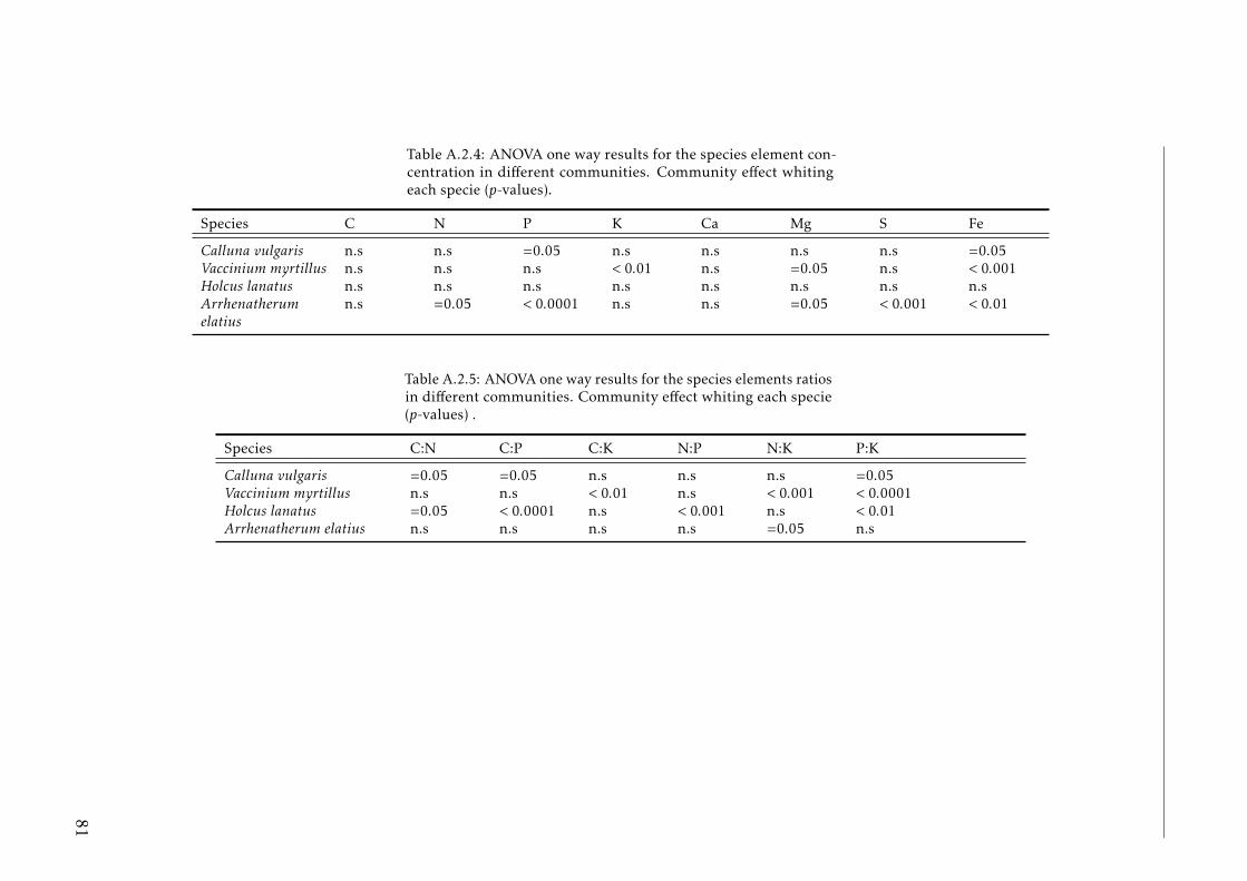
Table A.2.4: ANOVA one way results for the species element con-centration in different communities. Community effect whitingeach specie (p-values).
Species C N P K Ca Mg S Fe
Calluna vulgaris n.s n.s =0.05 n.s n.s n.s n.s =0.05Vaccinium myrtillus n.s n.s n.s < 0.01 n.s =0.05 n.s < 0.001Holcus lanatus n.s n.s n.s n.s n.s n.s n.s n.sArrhenatherumelatius
n.s =0.05 < 0.0001 n.s n.s =0.05 < 0.001 < 0.01
Table A.2.5: ANOVA one way results for the species elements ratiosin different communities. Community effect whiting each specie(p-values) .
Species C:N C:P C:K N:P N:K P:K
Calluna vulgaris =0.05 =0.05 n.s n.s n.s =0.05Vaccinium myrtillus n.s n.s < 0.01 n.s < 0.001 < 0.0001Holcus lanatus =0.05 < 0.0001 n.s < 0.001 n.s < 0.01Arrhenatherum elatius n.s n.s n.s n.s =0.05 n.s
81
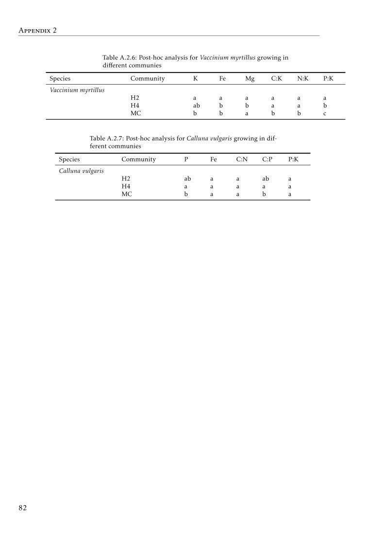
Appendix 2
Table A.2.6: Post-hoc analysis for Vaccinium myrtillus growing indifferent communies
Species Community K Fe Mg C:K N:K P:K
Vaccinium myrtillusH2 a a a a a aH4 ab b b a a bMC b b a b b c
Table A.2.7: Post-hoc analysis for Calluna vulgaris growing in dif-ferent communies
Species Community P Fe C:N C:P P:K
Calluna vulgarisH2 ab a a ab aH4 a a a a aMC b a a b a
82
Appendix 3: Chapter 3 -Encroachment of shrubs intosubalpine grasslands in the Pyreneeschanges the plant-soil stoichiometry
83
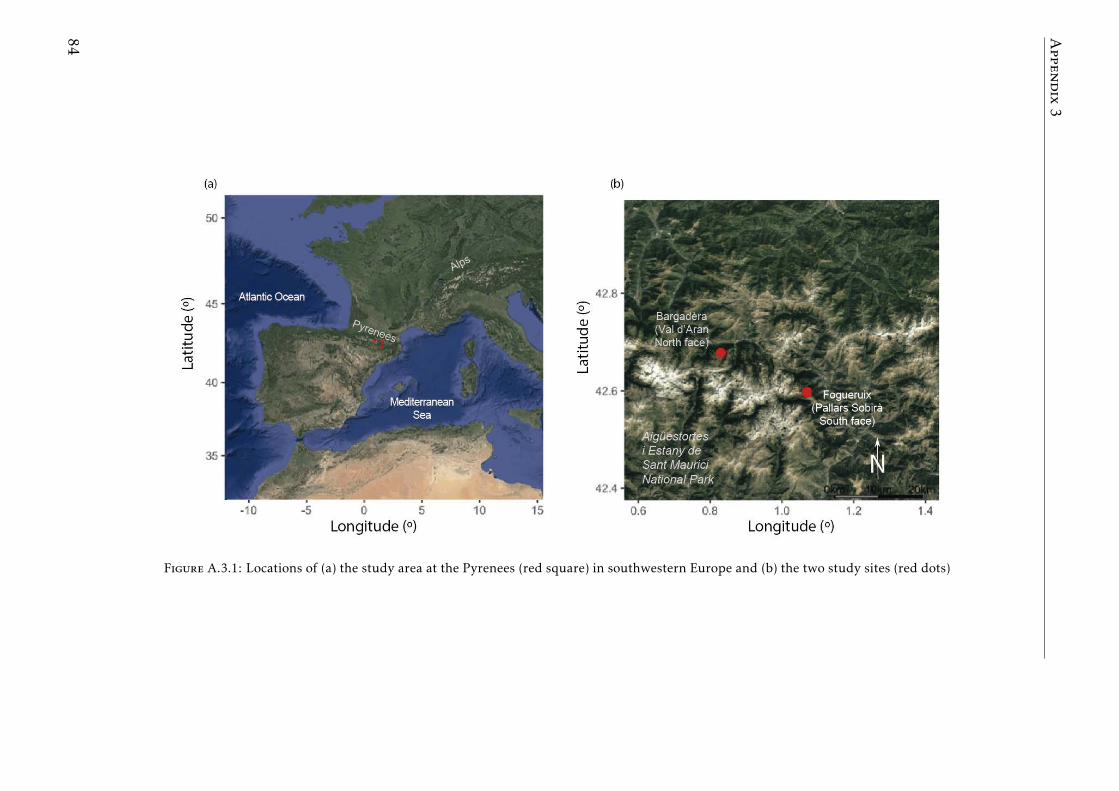
Appendix3
Figure A.3.1: Locations of (a) the study area at the Pyrenees (red square) in southwestern Europe and (b) the two study sites (red dots)
84
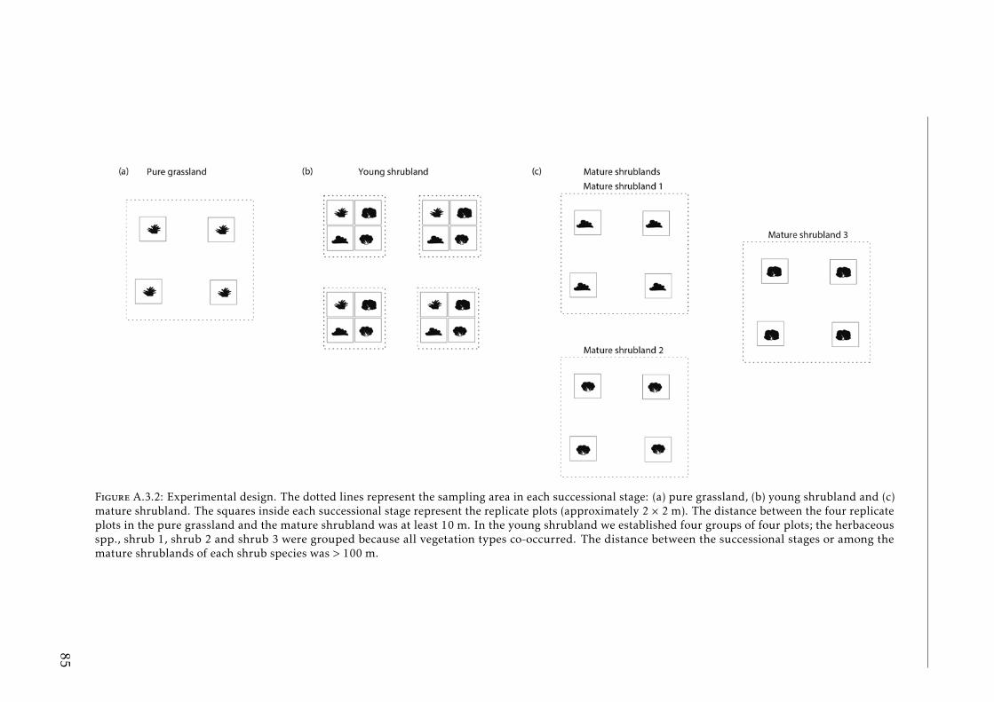
Figure A.3.2: Experimental design. The dotted lines represent the sampling area in each successional stage: (a) pure grassland, (b) young shrubland and (c)mature shrubland. The squares inside each successional stage represent the replicate plots (approximately 2 × 2 m). The distance between the four replicateplots in the pure grassland and the mature shrubland was at least 10 m. In the young shrubland we established four groups of four plots; the herbaceousspp., shrub 1, shrub 2 and shrub 3 were grouped because all vegetation types co-occurred. The distance between the successional stages or among themature shrublands of each shrub species was > 100 m.
85
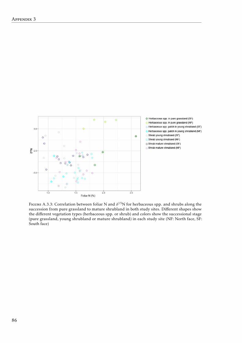
Appendix 3
Figure A.3.3: Correlation between foliar N and δ15N for herbaceous spp. and shrubs along thesuccession from pure grassland to mature shrubland in both study sites. Different shapes showthe different vegetation types (herbaceous spp. or shrub) and colors show the successional stage(pure grassland, young shrubland or mature shrubland) in each study site (NF: North face, SF:South face)
86
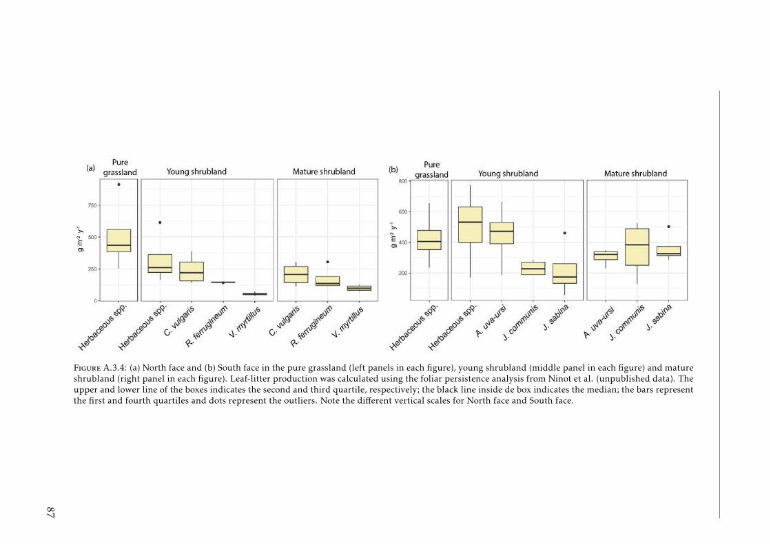
Figure A.3.4: (a) North face and (b) South face in the pure grassland (left panels in each figure), young shrubland (middle panel in each figure) and matureshrubland (right panel in each figure). Leaf-litter production was calculated using the foliar persistence analysis from Ninot et al. (unpublished data). Theupper and lower line of the boxes indicates the second and third quartile, respectively; the black line inside de box indicates the median; the bars representthe first and fourth quartiles and dots represent the outliers. Note the different vertical scales for North face and South face.
87
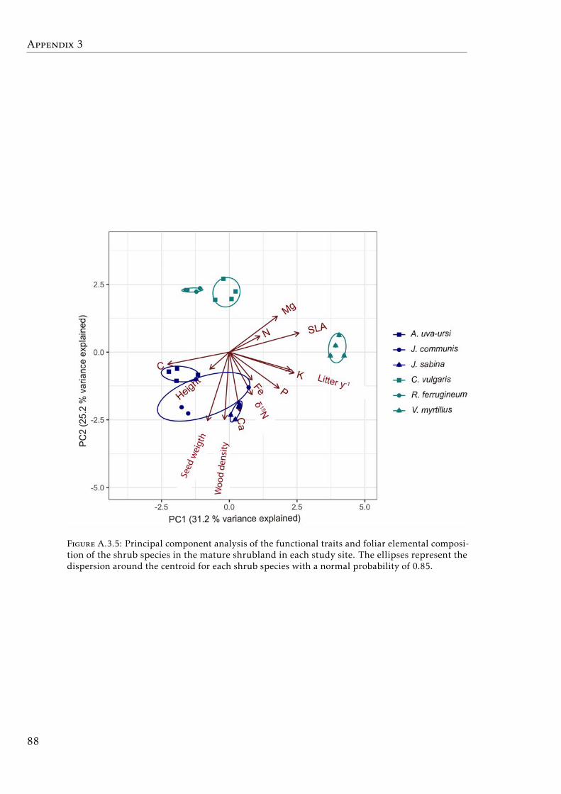
Appendix 3
Figure A.3.5: Principal component analysis of the functional traits and foliar elemental composi-tion of the shrub species in the mature shrubland in each study site. The ellipses represent thedispersion around the centroid for each shrub species with a normal probability of 0.85.
88
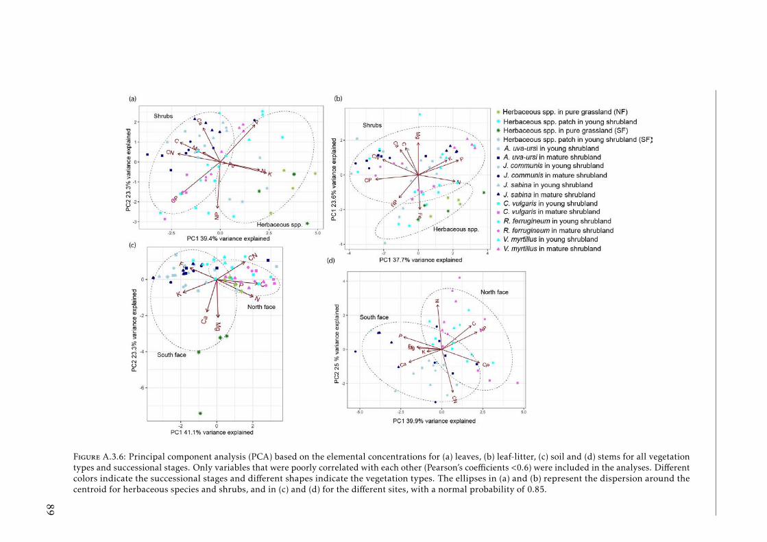
Figure A.3.6: Principal component analysis (PCA) based on the elemental concentrations for (a) leaves, (b) leaf-litter, (c) soil and (d) stems for all vegetationtypes and successional stages. Only variables that were poorly correlated with each other (Pearson’s coefficients <0.6) were included in the analyses. Differentcolors indicate the successional stages and different shapes indicate the vegetation types. The ellipses in (a) and (b) represent the dispersion around thecentroid for herbaceous species and shrubs, and in (c) and (d) for the different sites, with a normal probability of 0.85.
89
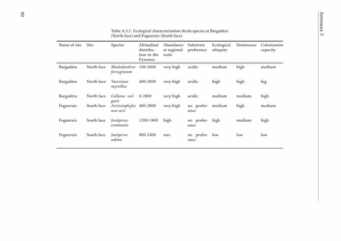
Appendix3Table A.3.1: Ecological characterization shrub species at Bargadera
(North face) and Fogueruix (South face).
Name of site Site Species Altitudinaldistribu-tion in thePyreenes
Abundanceat regionalscale
Substratepreference
Ecologicalubiquity
Dominance Colonizationcapacity
Bargadera North face Rhododendronferrugineum
100-2800 very high acidic medium high medium
Bargadera North face Vacciniunmyrtillus
400-2800 very high acidic high high hig
Bargadera North face Calluna vul-garis
0-2800 very high acidic medium medium high
Fogueruix South face Arctostaphylosuva-ursi
400-2800 very high no prefer-ence
medium high medium
Fogueruix South face Juniperuscommunis
1200-1800 high no prefer-ence
high medium high
Fogueruix South face Juniperussabina
800-2400 rare no prefer-ence
low low low
90
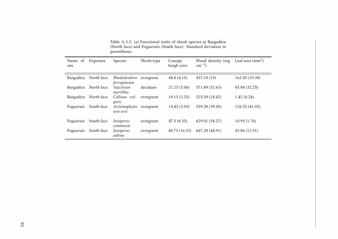
Table A.3.2: (a) Functional traits of shrub species at Bargadera(North face) and Fogueruix (South face). Standard deviation inparentheses.
Name ofsite
Exposure Species Shrub type Canopyheigh (cm)
Wood density (mgcm−3)
Leaf area (mm2)
Bargadera North face Rhododendronferrugineum
evergreen 44.8 (4.10) 457.18 (19) 162.45 (19.38)
Bargadera North face Vacciniunmyrtillus
deciduos 21.25 (3.06) 571.89 (32.63) 85.88 (32.25)
Bargadera North face Calluna vul-garis
evergreen 19.15 (3.25) 525.59 (24.42) 1.42 (0.24)
Fogueruix South face Arctostaphylosuva-ursi
evergreen 14.45 (3.03) 539.38 (39.45) 126.55 (41.05)
Fogueruix South face Juniperuscommunis
evergreen 47.5 (8.35) 629.01 (54.27) 10.95 (1.76)
Fogueruix South face Juniperussabina
evergreen 40.73 (16.33) 667.28 (44.91) 43.06 (12.91)
91
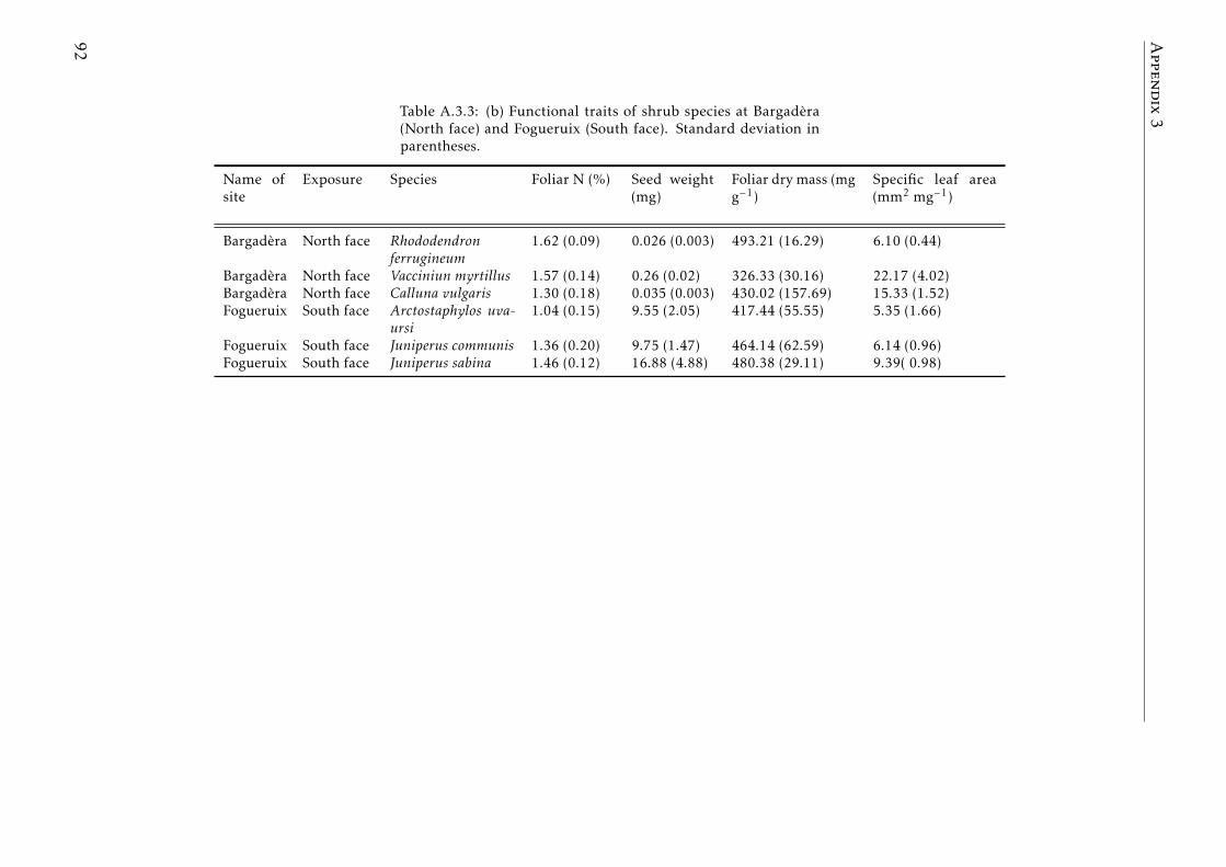
Appendix3Table A.3.3: (b) Functional traits of shrub species at Bargadera
(North face) and Fogueruix (South face). Standard deviation inparentheses.
Name ofsite
Exposure Species Foliar N (%) Seed weight(mg)
Foliar dry mass (mgg−1)
Specific leaf area(mm2 mg−1)
Bargadera North face Rhododendronferrugineum
1.62 (0.09) 0.026 (0.003) 493.21 (16.29) 6.10 (0.44)
Bargadera North face Vacciniun myrtillus 1.57 (0.14) 0.26 (0.02) 326.33 (30.16) 22.17 (4.02)Bargadera North face Calluna vulgaris 1.30 (0.18) 0.035 (0.003) 430.02 (157.69) 15.33 (1.52)Fogueruix South face Arctostaphylos uva-
ursi1.04 (0.15) 9.55 (2.05) 417.44 (55.55) 5.35 (1.66)
Fogueruix South face Juniperus communis 1.36 (0.20) 9.75 (1.47) 464.14 (62.59) 6.14 (0.96)Fogueruix South face Juniperus sabina 1.46 (0.12) 16.88 (4.88) 480.38 (29.11) 9.39( 0.98)
92
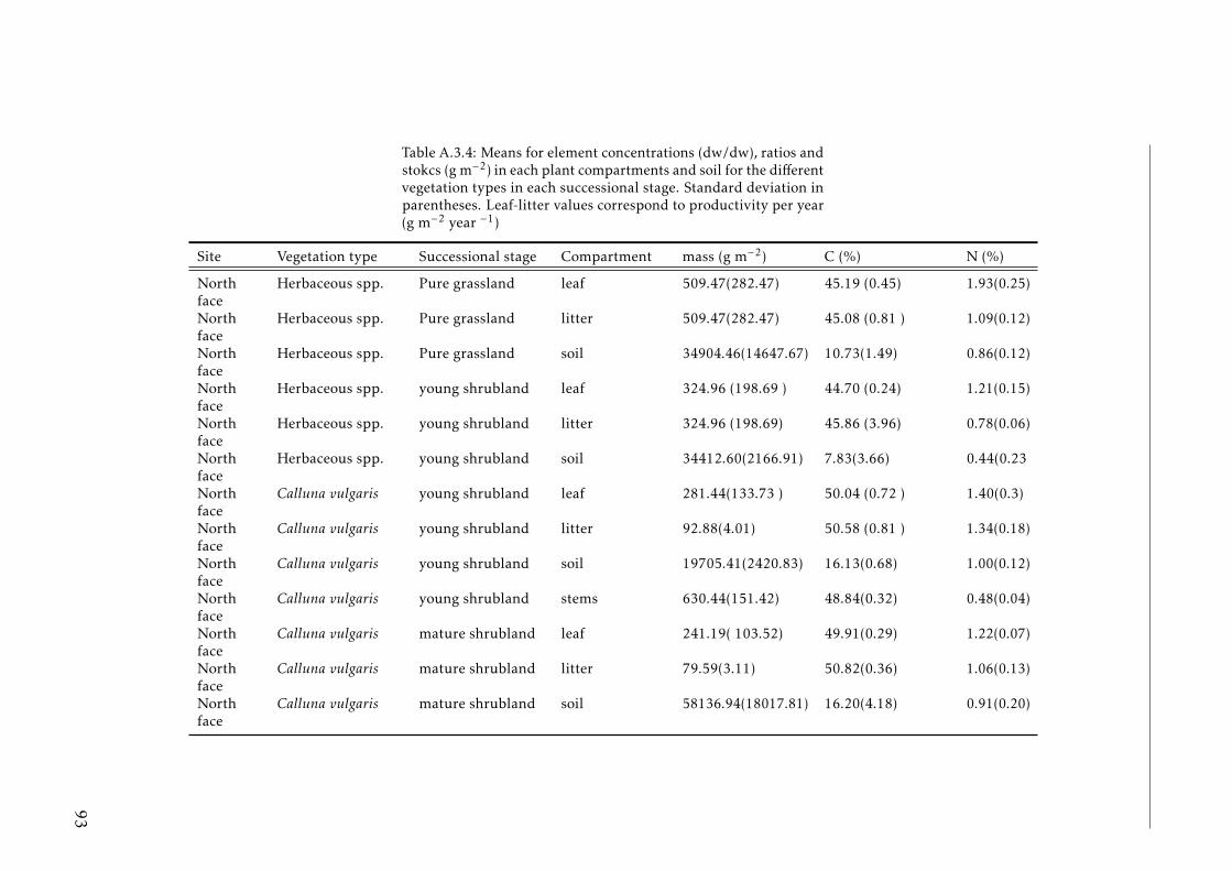
Table A.3.4: Means for element concentrations (dw/dw), ratios andstokcs (g m−2) in each plant compartments and soil for the differentvegetation types in each successional stage. Standard deviation inparentheses. Leaf-litter values correspond to productivity per year(g m−2 year −1)
Site Vegetation type Successional stage Compartment mass (g m−2) C (%) N (%)
Northface
Herbaceous spp. Pure grassland leaf 509.47(282.47) 45.19 (0.45) 1.93(0.25)
Northface
Herbaceous spp. Pure grassland litter 509.47(282.47) 45.08 (0.81 ) 1.09(0.12)
Northface
Herbaceous spp. Pure grassland soil 34904.46(14647.67) 10.73(1.49) 0.86(0.12)
Northface
Herbaceous spp. young shrubland leaf 324.96 (198.69 ) 44.70 (0.24) 1.21(0.15)
Northface
Herbaceous spp. young shrubland litter 324.96 (198.69) 45.86 (3.96) 0.78(0.06)
Northface
Herbaceous spp. young shrubland soil 34412.60(2166.91) 7.83(3.66) 0.44(0.23
Northface
Calluna vulgaris young shrubland leaf 281.44(133.73 ) 50.04 (0.72 ) 1.40(0.3)
Northface
Calluna vulgaris young shrubland litter 92.88(4.01) 50.58 (0.81 ) 1.34(0.18)
Northface
Calluna vulgaris young shrubland soil 19705.41(2420.83) 16.13(0.68) 1.00(0.12)
Northface
Calluna vulgaris young shrubland stems 630.44(151.42) 48.84(0.32) 0.48(0.04)
Northface
Calluna vulgaris mature shrubland leaf 241.19( 103.52) 49.91(0.29) 1.22(0.07)
Northface
Calluna vulgaris mature shrubland litter 79.59(3.11) 50.82(0.36) 1.06(0.13)
Northface
Calluna vulgaris mature shrubland soil 58136.94(18017.81) 16.20(4.18) 0.91(0.20)
93
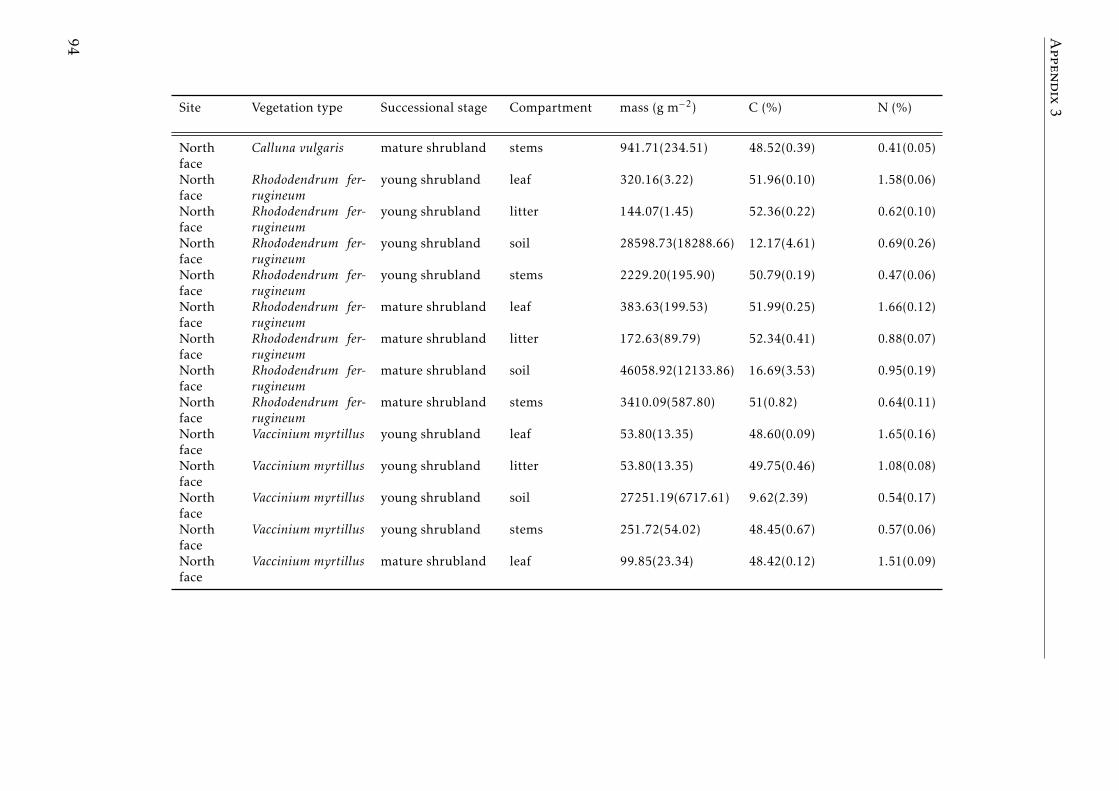
Appendix3Site Vegetation type Successional stage Compartment mass (g m−2) C (%) N (%)
Northface
Calluna vulgaris mature shrubland stems 941.71(234.51) 48.52(0.39) 0.41(0.05)
Northface
Rhododendrum fer-rugineum
young shrubland leaf 320.16(3.22) 51.96(0.10) 1.58(0.06)
Northface
Rhododendrum fer-rugineum
young shrubland litter 144.07(1.45) 52.36(0.22) 0.62(0.10)
Northface
Rhododendrum fer-rugineum
young shrubland soil 28598.73(18288.66) 12.17(4.61) 0.69(0.26)
Northface
Rhododendrum fer-rugineum
young shrubland stems 2229.20(195.90) 50.79(0.19) 0.47(0.06)
Northface
Rhododendrum fer-rugineum
mature shrubland leaf 383.63(199.53) 51.99(0.25) 1.66(0.12)
Northface
Rhododendrum fer-rugineum
mature shrubland litter 172.63(89.79) 52.34(0.41) 0.88(0.07)
Northface
Rhododendrum fer-rugineum
mature shrubland soil 46058.92(12133.86) 16.69(3.53) 0.95(0.19)
Northface
Rhododendrum fer-rugineum
mature shrubland stems 3410.09(587.80) 51(0.82) 0.64(0.11)
Northface
Vaccinium myrtillus young shrubland leaf 53.80(13.35) 48.60(0.09) 1.65(0.16)
Northface
Vaccinium myrtillus young shrubland litter 53.80(13.35) 49.75(0.46) 1.08(0.08)
Northface
Vaccinium myrtillus young shrubland soil 27251.19(6717.61) 9.62(2.39) 0.54(0.17)
Northface
Vaccinium myrtillus young shrubland stems 251.72(54.02) 48.45(0.67) 0.57(0.06)
Northface
Vaccinium myrtillus mature shrubland leaf 99.85(23.34) 48.42(0.12) 1.51(0.09)
94
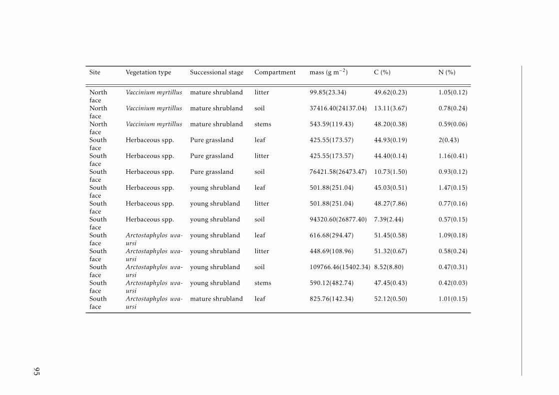
Site Vegetation type Successional stage Compartment mass (g m−2) C (%) N (%)
Northface
Vaccinium myrtillus mature shrubland litter 99.85(23.34) 49.62(0.23) 1.05(0.12)
Northface
Vaccinium myrtillus mature shrubland soil 37416.40(24137.04) 13.11(3.67) 0.78(0.24)
Northface
Vaccinium myrtillus mature shrubland stems 543.59(119.43) 48.20(0.38) 0.59(0.06)
Southface
Herbaceous spp. Pure grassland leaf 425.55(173.57) 44.93(0.19) 2(0.43)
Southface
Herbaceous spp. Pure grassland litter 425.55(173.57) 44.40(0.14) 1.16(0.41)
Southface
Herbaceous spp. Pure grassland soil 76421.58(26473.47) 10.73(1.50) 0.93(0.12)
Southface
Herbaceous spp. young shrubland leaf 501.88(251.04) 45.03(0.51) 1.47(0.15)
Southface
Herbaceous spp. young shrubland litter 501.88(251.04) 48.27(7.86) 0.77(0.16)
Southface
Herbaceous spp. young shrubland soil 94320.60(26877.40) 7.39(2.44) 0.57(0.15)
Southface
Arctostaphylos uva-ursi
young shrubland leaf 616.68(294.47) 51.45(0.58) 1.09(0.18)
Southface
Arctostaphylos uva-ursi
young shrubland litter 448.69(108.96) 51.32(0.67) 0.58(0.24)
Southface
Arctostaphylos uva-ursi
young shrubland soil 109766.46(15402.34) 8.52(8.80) 0.47(0.31)
Southface
Arctostaphylos uva-ursi
young shrubland stems 590.12(482.74) 47.45(0.43) 0.42(0.03)
Southface
Arctostaphylos uva-ursi
mature shrubland leaf 825.76(142.34) 52.12(0.50) 1.01(0.15)
95
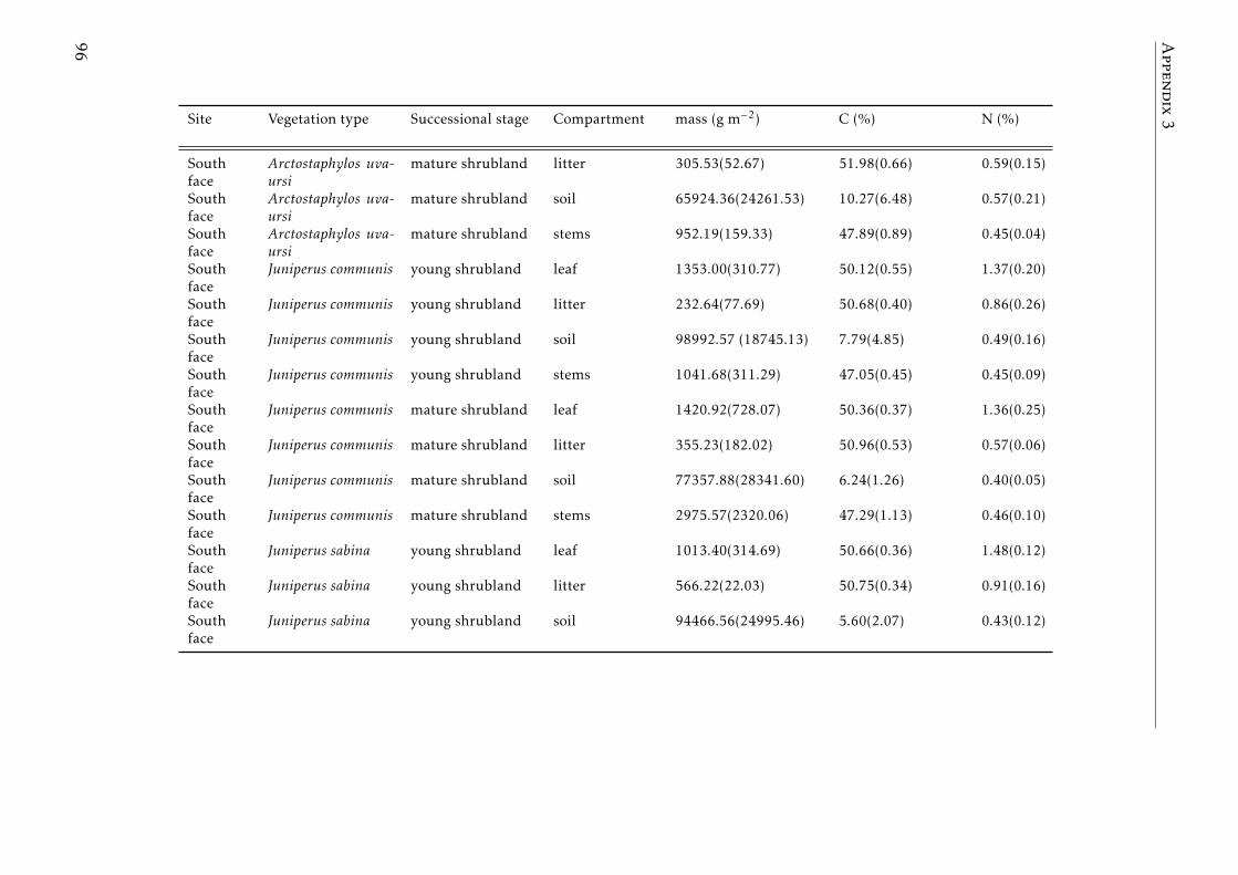
Appendix3Site Vegetation type Successional stage Compartment mass (g m−2) C (%) N (%)
Southface
Arctostaphylos uva-ursi
mature shrubland litter 305.53(52.67) 51.98(0.66) 0.59(0.15)
Southface
Arctostaphylos uva-ursi
mature shrubland soil 65924.36(24261.53) 10.27(6.48) 0.57(0.21)
Southface
Arctostaphylos uva-ursi
mature shrubland stems 952.19(159.33) 47.89(0.89) 0.45(0.04)
Southface
Juniperus communis young shrubland leaf 1353.00(310.77) 50.12(0.55) 1.37(0.20)
Southface
Juniperus communis young shrubland litter 232.64(77.69) 50.68(0.40) 0.86(0.26)
Southface
Juniperus communis young shrubland soil 98992.57 (18745.13) 7.79(4.85) 0.49(0.16)
Southface
Juniperus communis young shrubland stems 1041.68(311.29) 47.05(0.45) 0.45(0.09)
Southface
Juniperus communis mature shrubland leaf 1420.92(728.07) 50.36(0.37) 1.36(0.25)
Southface
Juniperus communis mature shrubland litter 355.23(182.02) 50.96(0.53) 0.57(0.06)
Southface
Juniperus communis mature shrubland soil 77357.88(28341.60) 6.24(1.26) 0.40(0.05)
Southface
Juniperus communis mature shrubland stems 2975.57(2320.06) 47.29(1.13) 0.46(0.10)
Southface
Juniperus sabina young shrubland leaf 1013.40(314.69) 50.66(0.36) 1.48(0.12)
Southface
Juniperus sabina young shrubland litter 566.22(22.03) 50.75(0.34) 0.91(0.16)
Southface
Juniperus sabina young shrubland soil 94466.56(24995.46) 5.60(2.07) 0.43(0.12)
96
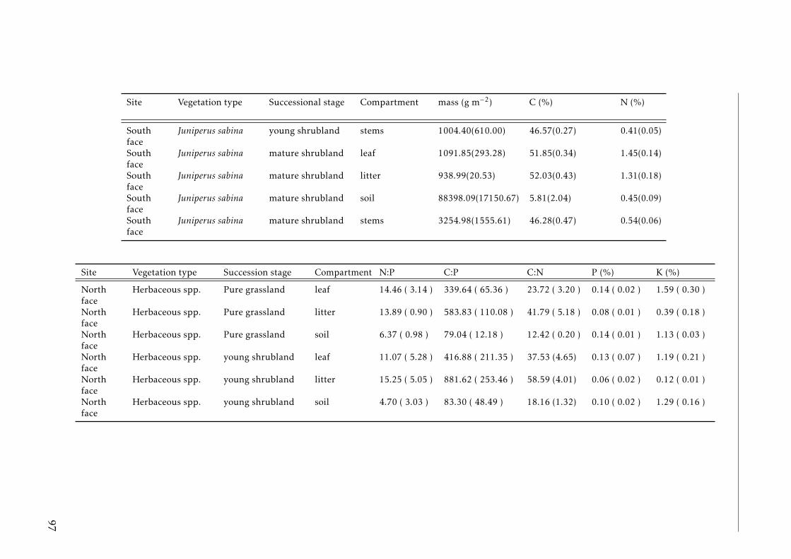
Site Vegetation type Successional stage Compartment mass (g m−2) C (%) N (%)
Southface
Juniperus sabina young shrubland stems 1004.40(610.00) 46.57(0.27) 0.41(0.05)
Southface
Juniperus sabina mature shrubland leaf 1091.85(293.28) 51.85(0.34) 1.45(0.14)
Southface
Juniperus sabina mature shrubland litter 938.99(20.53) 52.03(0.43) 1.31(0.18)
Southface
Juniperus sabina mature shrubland soil 88398.09(17150.67) 5.81(2.04) 0.45(0.09)
Southface
Juniperus sabina mature shrubland stems 3254.98(1555.61) 46.28(0.47) 0.54(0.06)
Site Vegetation type Succession stage Compartment N:P C:P C:N P (%) K (%)
Northface
Herbaceous spp. Pure grassland leaf 14.46 ( 3.14 ) 339.64 ( 65.36 ) 23.72 ( 3.20 ) 0.14 ( 0.02 ) 1.59 ( 0.30 )
Northface
Herbaceous spp. Pure grassland litter 13.89 ( 0.90 ) 583.83 ( 110.08 ) 41.79 ( 5.18 ) 0.08 ( 0.01 ) 0.39 ( 0.18 )
Northface
Herbaceous spp. Pure grassland soil 6.37 ( 0.98 ) 79.04 ( 12.18 ) 12.42 ( 0.20 ) 0.14 ( 0.01 ) 1.13 ( 0.03 )
Northface
Herbaceous spp. young shrubland leaf 11.07 ( 5.28 ) 416.88 ( 211.35 ) 37.53 (4.65) 0.13 ( 0.07 ) 1.19 ( 0.21 )
Northface
Herbaceous spp. young shrubland litter 15.25 ( 5.05 ) 881.62 ( 253.46 ) 58.59 (4.01) 0.06 ( 0.02 ) 0.12 ( 0.01 )
Northface
Herbaceous spp. young shrubland soil 4.70 ( 3.03 ) 83.30 ( 48.49 ) 18.16 (1.32) 0.10 ( 0.02 ) 1.29 ( 0.16 )
97
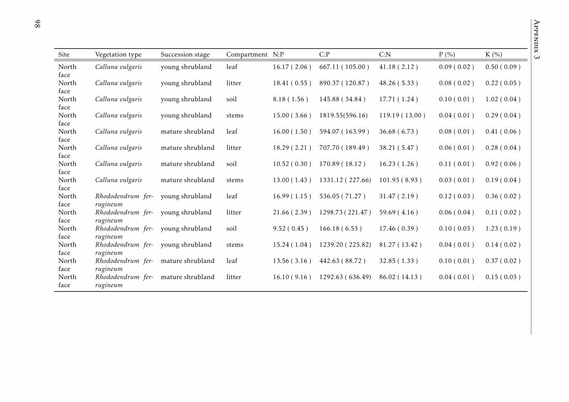
Appendix3Site Vegetation type Succession stage Compartment N:P C:P C:N P (%) K (%)
Northface
Calluna vulgaris young shrubland leaf 16.17 ( 2.06 ) 667.11 ( 105.00 ) 41.18 ( 2.12 ) 0.09 ( 0.02 ) 0.50 ( 0.09 )
Northface
Calluna vulgaris young shrubland litter 18.41 ( 0.55 ) 890.37 ( 120.87 ) 48.26 ( 5.33 ) 0.08 ( 0.02 ) 0.22 ( 0.05 )
Northface
Calluna vulgaris young shrubland soil 8.18 ( 1.56 ) 145.88 ( 34.84 ) 17.71 ( 1.24 ) 0.10 ( 0.01 ) 1.02 ( 0.04 )
Northface
Calluna vulgaris young shrubland stems 15.00 ( 3.66 ) 1819.55(596.16) 119.19 ( 13.00 ) 0.04 ( 0.01 ) 0.29 ( 0.04 )
Northface
Calluna vulgaris mature shrubland leaf 16.00 ( 1.50 ) 594.07 ( 163.99 ) 36.68 ( 6.73 ) 0.08 ( 0.01 ) 0.41 ( 0.06 )
Northface
Calluna vulgaris mature shrubland litter 18.29 ( 2.21 ) 707.70 ( 189.49 ) 38.21 ( 5.47 ) 0.06 ( 0.01 ) 0.28 ( 0.04 )
Northface
Calluna vulgaris mature shrubland soil 10.52 ( 0.30 ) 170.89 ( 18.12 ) 16.23 ( 1.26 ) 0.11 ( 0.01 ) 0.92 ( 0.06 )
Northface
Calluna vulgaris mature shrubland stems 13.00 ( 1.43 ) 1331.12 ( 227.66) 101.93 ( 8.93 ) 0.03 ( 0.01 ) 0.19 ( 0.04 )
Northface
Rhododendrum fer-rugineum
young shrubland leaf 16.99 ( 1.15 ) 536.05 ( 71.27 ) 31.47 ( 2.19 ) 0.12 ( 0.03 ) 0.36 ( 0.02 )
Northface
Rhododendrum fer-rugineum
young shrubland litter 21.66 ( 2.39 ) 1298.73 ( 221.47 ) 59.69 ( 4.16 ) 0.06 ( 0.04 ) 0.11 ( 0.02 )
Northface
Rhododendrum fer-rugineum
young shrubland soil 9.52 ( 0.45 ) 166.18 ( 6.53 ) 17.46 ( 0.39 ) 0.10 ( 0.03 ) 1.23 ( 0.19 )
Northface
Rhododendrum fer-rugineum
young shrubland stems 15.24 ( 1.04 ) 1239.20 ( 225.82) 81.27 ( 13.42 ) 0.04 ( 0.01 ) 0.14 ( 0.02 )
Northface
Rhododendrum fer-rugineum
mature shrubland leaf 13.56 ( 3.16 ) 442.63 ( 88.72 ) 32.85 ( 1.33 ) 0.10 ( 0.01 ) 0.37 ( 0.02 )
Northface
Rhododendrum fer-rugineum
mature shrubland litter 16.10 ( 9.16 ) 1292.63 ( 636.49) 86.02 ( 14.13 ) 0.04 ( 0.01 ) 0.15 ( 0.03 )
98
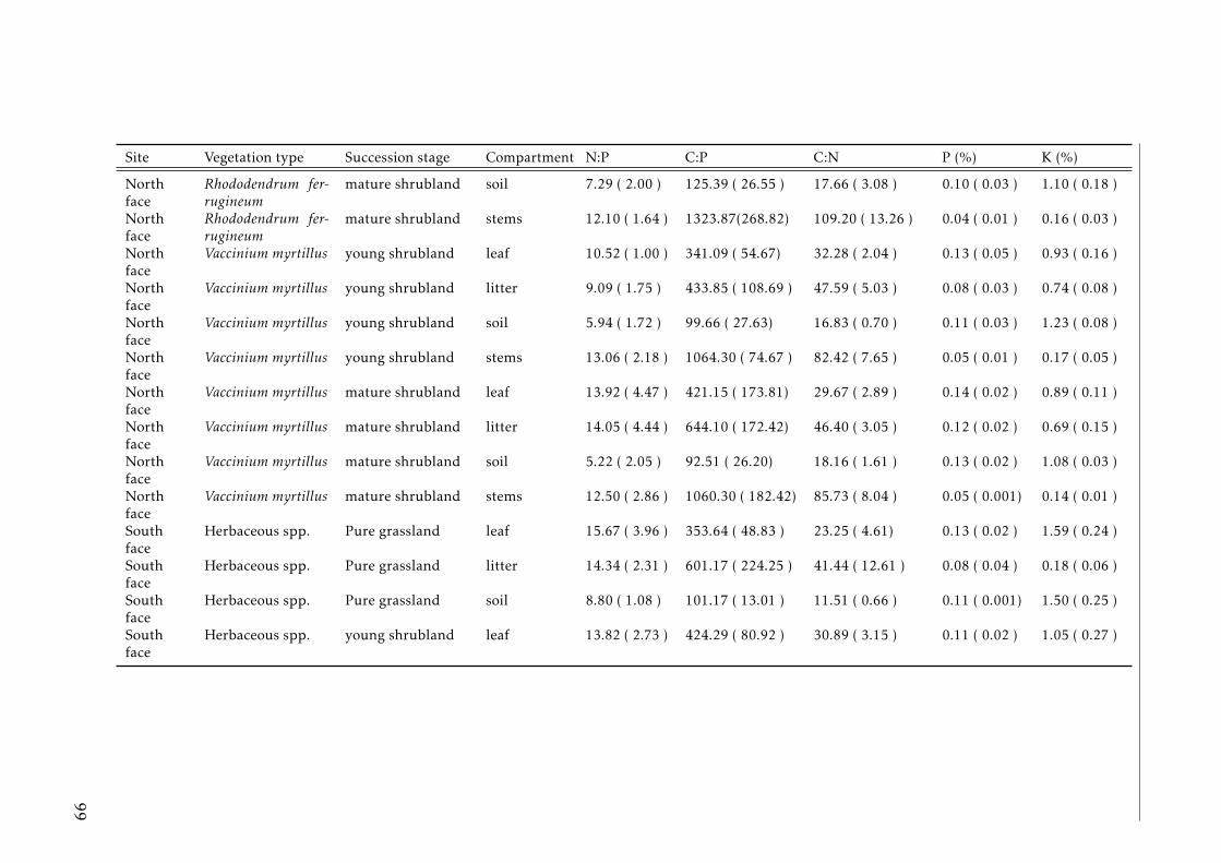
Site Vegetation type Succession stage Compartment N:P C:P C:N P (%) K (%)
Northface
Rhododendrum fer-rugineum
mature shrubland soil 7.29 ( 2.00 ) 125.39 ( 26.55 ) 17.66 ( 3.08 ) 0.10 ( 0.03 ) 1.10 ( 0.18 )
Northface
Rhododendrum fer-rugineum
mature shrubland stems 12.10 ( 1.64 ) 1323.87(268.82) 109.20 ( 13.26 ) 0.04 ( 0.01 ) 0.16 ( 0.03 )
Northface
Vaccinium myrtillus young shrubland leaf 10.52 ( 1.00 ) 341.09 ( 54.67) 32.28 ( 2.04 ) 0.13 ( 0.05 ) 0.93 ( 0.16 )
Northface
Vaccinium myrtillus young shrubland litter 9.09 ( 1.75 ) 433.85 ( 108.69 ) 47.59 ( 5.03 ) 0.08 ( 0.03 ) 0.74 ( 0.08 )
Northface
Vaccinium myrtillus young shrubland soil 5.94 ( 1.72 ) 99.66 ( 27.63) 16.83 ( 0.70 ) 0.11 ( 0.03 ) 1.23 ( 0.08 )
Northface
Vaccinium myrtillus young shrubland stems 13.06 ( 2.18 ) 1064.30 ( 74.67 ) 82.42 ( 7.65 ) 0.05 ( 0.01 ) 0.17 ( 0.05 )
Northface
Vaccinium myrtillus mature shrubland leaf 13.92 ( 4.47 ) 421.15 ( 173.81) 29.67 ( 2.89 ) 0.14 ( 0.02 ) 0.89 ( 0.11 )
Northface
Vaccinium myrtillus mature shrubland litter 14.05 ( 4.44 ) 644.10 ( 172.42) 46.40 ( 3.05 ) 0.12 ( 0.02 ) 0.69 ( 0.15 )
Northface
Vaccinium myrtillus mature shrubland soil 5.22 ( 2.05 ) 92.51 ( 26.20) 18.16 ( 1.61 ) 0.13 ( 0.02 ) 1.08 ( 0.03 )
Northface
Vaccinium myrtillus mature shrubland stems 12.50 ( 2.86 ) 1060.30 ( 182.42) 85.73 ( 8.04 ) 0.05 ( 0.001) 0.14 ( 0.01 )
Southface
Herbaceous spp. Pure grassland leaf 15.67 ( 3.96 ) 353.64 ( 48.83 ) 23.25 ( 4.61) 0.13 ( 0.02 ) 1.59 ( 0.24 )
Southface
Herbaceous spp. Pure grassland litter 14.34 ( 2.31 ) 601.17 ( 224.25 ) 41.44 ( 12.61 ) 0.08 ( 0.04 ) 0.18 ( 0.06 )
Southface
Herbaceous spp. Pure grassland soil 8.80 ( 1.08 ) 101.17 ( 13.01 ) 11.51 ( 0.66 ) 0.11 ( 0.001) 1.50 ( 0.25 )
Southface
Herbaceous spp. young shrubland leaf 13.82 ( 2.73 ) 424.29 ( 80.92 ) 30.89 ( 3.15 ) 0.11 ( 0.02 ) 1.05 ( 0.27 )
99
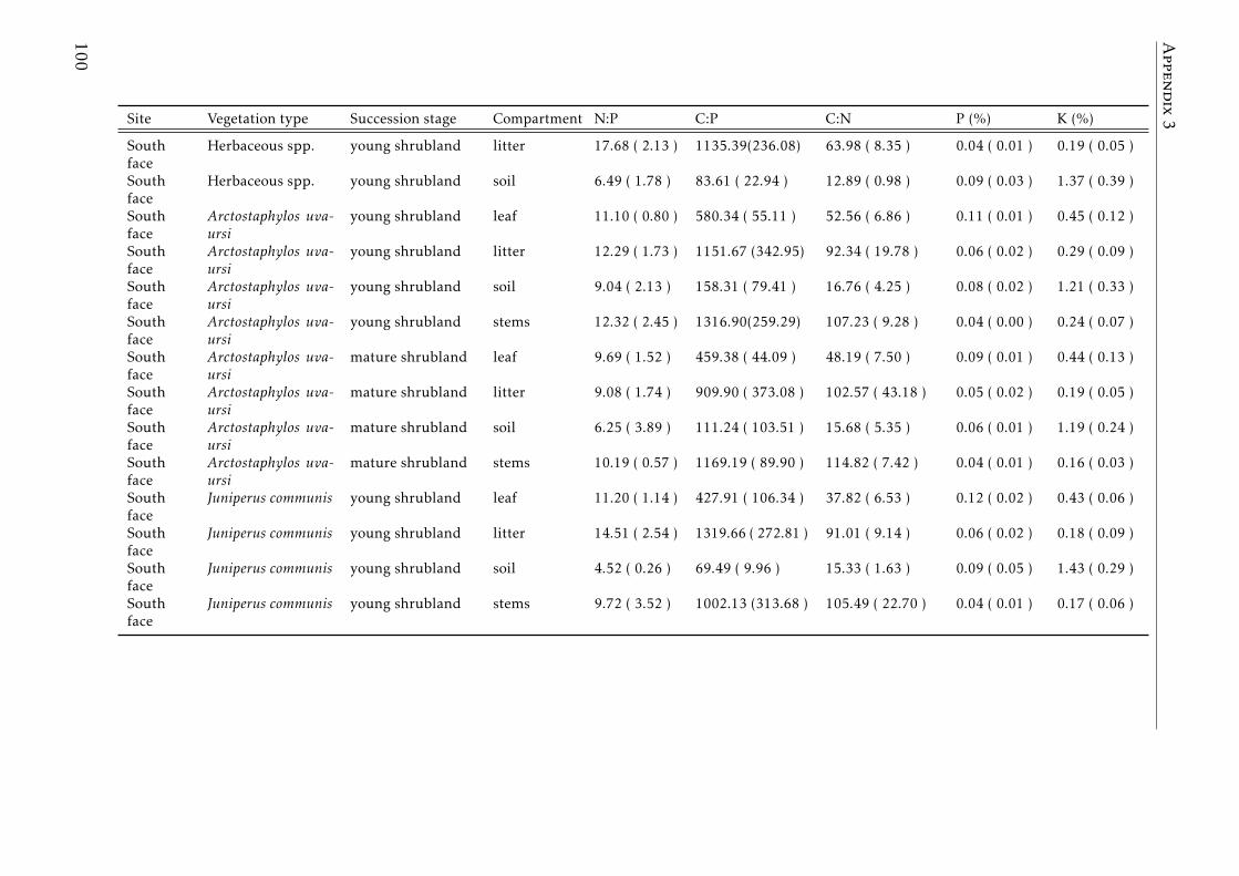
Appendix3Site Vegetation type Succession stage Compartment N:P C:P C:N P (%) K (%)
Southface
Herbaceous spp. young shrubland litter 17.68 ( 2.13 ) 1135.39(236.08) 63.98 ( 8.35 ) 0.04 ( 0.01 ) 0.19 ( 0.05 )
Southface
Herbaceous spp. young shrubland soil 6.49 ( 1.78 ) 83.61 ( 22.94 ) 12.89 ( 0.98 ) 0.09 ( 0.03 ) 1.37 ( 0.39 )
Southface
Arctostaphylos uva-ursi
young shrubland leaf 11.10 ( 0.80 ) 580.34 ( 55.11 ) 52.56 ( 6.86 ) 0.11 ( 0.01 ) 0.45 ( 0.12 )
Southface
Arctostaphylos uva-ursi
young shrubland litter 12.29 ( 1.73 ) 1151.67 (342.95) 92.34 ( 19.78 ) 0.06 ( 0.02 ) 0.29 ( 0.09 )
Southface
Arctostaphylos uva-ursi
young shrubland soil 9.04 ( 2.13 ) 158.31 ( 79.41 ) 16.76 ( 4.25 ) 0.08 ( 0.02 ) 1.21 ( 0.33 )
Southface
Arctostaphylos uva-ursi
young shrubland stems 12.32 ( 2.45 ) 1316.90(259.29) 107.23 ( 9.28 ) 0.04 ( 0.00 ) 0.24 ( 0.07 )
Southface
Arctostaphylos uva-ursi
mature shrubland leaf 9.69 ( 1.52 ) 459.38 ( 44.09 ) 48.19 ( 7.50 ) 0.09 ( 0.01 ) 0.44 ( 0.13 )
Southface
Arctostaphylos uva-ursi
mature shrubland litter 9.08 ( 1.74 ) 909.90 ( 373.08 ) 102.57 ( 43.18 ) 0.05 ( 0.02 ) 0.19 ( 0.05 )
Southface
Arctostaphylos uva-ursi
mature shrubland soil 6.25 ( 3.89 ) 111.24 ( 103.51 ) 15.68 ( 5.35 ) 0.06 ( 0.01 ) 1.19 ( 0.24 )
Southface
Arctostaphylos uva-ursi
mature shrubland stems 10.19 ( 0.57 ) 1169.19 ( 89.90 ) 114.82 ( 7.42 ) 0.04 ( 0.01 ) 0.16 ( 0.03 )
Southface
Juniperus communis young shrubland leaf 11.20 ( 1.14 ) 427.91 ( 106.34 ) 37.82 ( 6.53 ) 0.12 ( 0.02 ) 0.43 ( 0.06 )
Southface
Juniperus communis young shrubland litter 14.51 ( 2.54 ) 1319.66 ( 272.81 ) 91.01 ( 9.14 ) 0.06 ( 0.02 ) 0.18 ( 0.09 )
Southface
Juniperus communis young shrubland soil 4.52 ( 0.26 ) 69.49 ( 9.96 ) 15.33 ( 1.63 ) 0.09 ( 0.05 ) 1.43 ( 0.29 )
Southface
Juniperus communis young shrubland stems 9.72 ( 3.52 ) 1002.13 (313.68 ) 105.49 ( 22.70 ) 0.04 ( 0.01 ) 0.17 ( 0.06 )
100
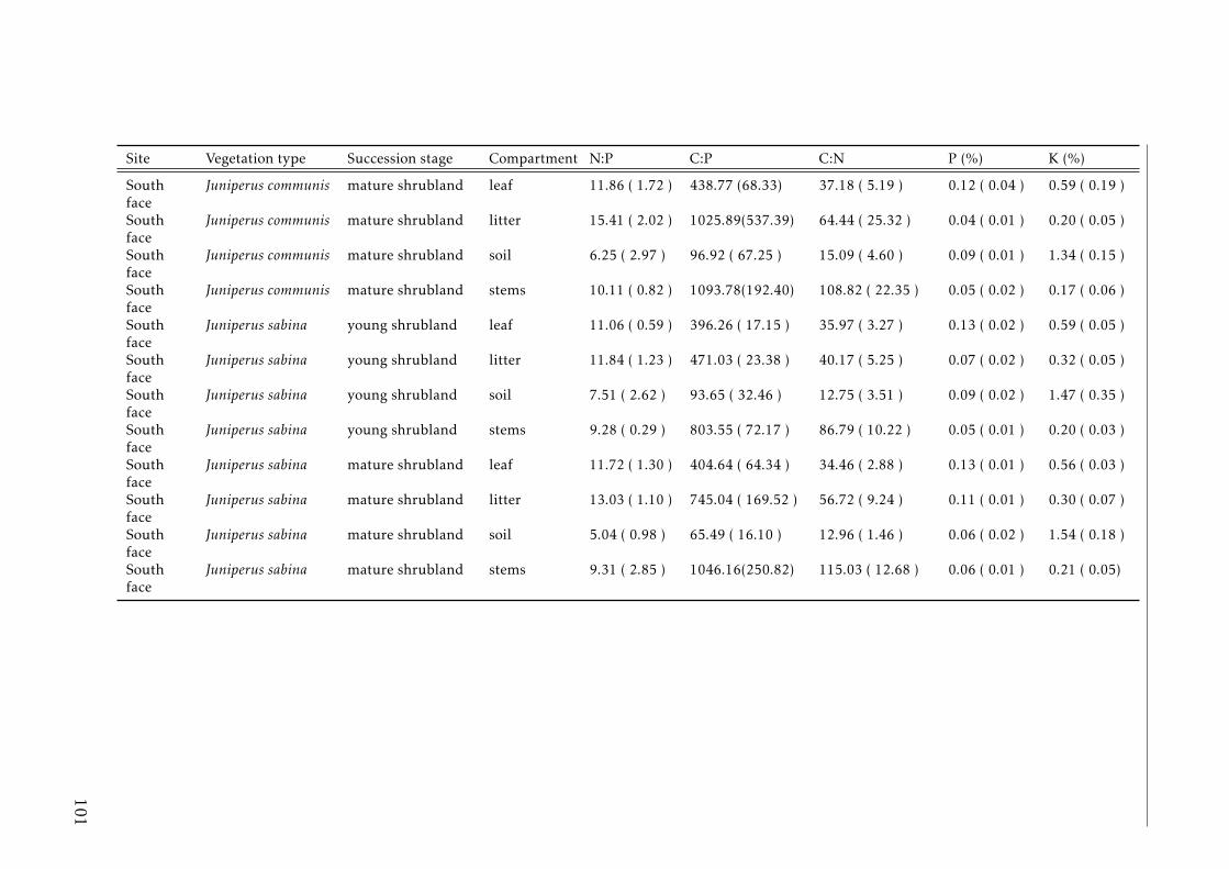
Site Vegetation type Succession stage Compartment N:P C:P C:N P (%) K (%)
Southface
Juniperus communis mature shrubland leaf 11.86 ( 1.72 ) 438.77 (68.33) 37.18 ( 5.19 ) 0.12 ( 0.04 ) 0.59 ( 0.19 )
Southface
Juniperus communis mature shrubland litter 15.41 ( 2.02 ) 1025.89(537.39) 64.44 ( 25.32 ) 0.04 ( 0.01 ) 0.20 ( 0.05 )
Southface
Juniperus communis mature shrubland soil 6.25 ( 2.97 ) 96.92 ( 67.25 ) 15.09 ( 4.60 ) 0.09 ( 0.01 ) 1.34 ( 0.15 )
Southface
Juniperus communis mature shrubland stems 10.11 ( 0.82 ) 1093.78(192.40) 108.82 ( 22.35 ) 0.05 ( 0.02 ) 0.17 ( 0.06 )
Southface
Juniperus sabina young shrubland leaf 11.06 ( 0.59 ) 396.26 ( 17.15 ) 35.97 ( 3.27 ) 0.13 ( 0.02 ) 0.59 ( 0.05 )
Southface
Juniperus sabina young shrubland litter 11.84 ( 1.23 ) 471.03 ( 23.38 ) 40.17 ( 5.25 ) 0.07 ( 0.02 ) 0.32 ( 0.05 )
Southface
Juniperus sabina young shrubland soil 7.51 ( 2.62 ) 93.65 ( 32.46 ) 12.75 ( 3.51 ) 0.09 ( 0.02 ) 1.47 ( 0.35 )
Southface
Juniperus sabina young shrubland stems 9.28 ( 0.29 ) 803.55 ( 72.17 ) 86.79 ( 10.22 ) 0.05 ( 0.01 ) 0.20 ( 0.03 )
Southface
Juniperus sabina mature shrubland leaf 11.72 ( 1.30 ) 404.64 ( 64.34 ) 34.46 ( 2.88 ) 0.13 ( 0.01 ) 0.56 ( 0.03 )
Southface
Juniperus sabina mature shrubland litter 13.03 ( 1.10 ) 745.04 ( 169.52 ) 56.72 ( 9.24 ) 0.11 ( 0.01 ) 0.30 ( 0.07 )
Southface
Juniperus sabina mature shrubland soil 5.04 ( 0.98 ) 65.49 ( 16.10 ) 12.96 ( 1.46 ) 0.06 ( 0.02 ) 1.54 ( 0.18 )
Southface
Juniperus sabina mature shrubland stems 9.31 ( 2.85 ) 1046.16(250.82) 115.03 ( 12.68 ) 0.06 ( 0.01 ) 0.21 ( 0.05)
101
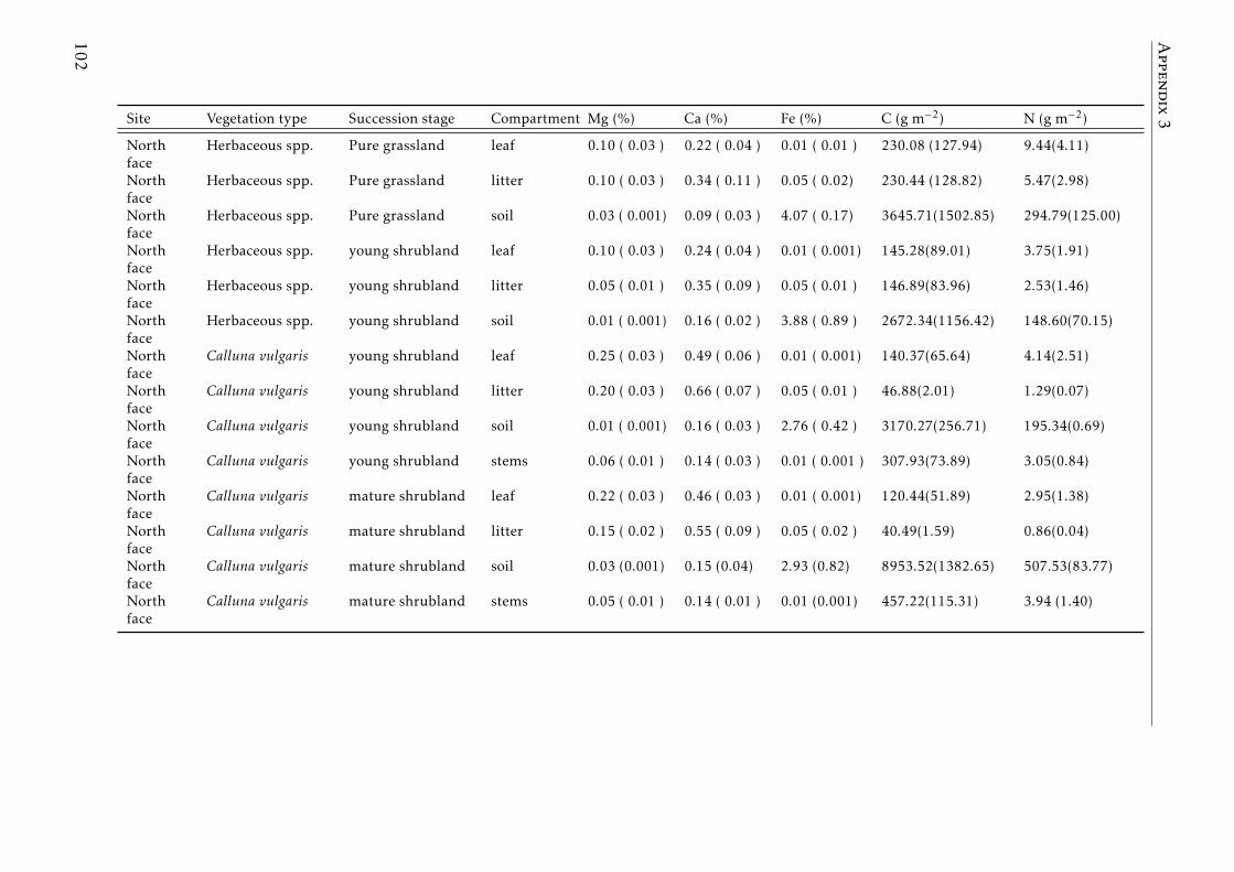
Appendix3Site Vegetation type Succession stage Compartment Mg (%) Ca (%) Fe (%) C (g m−2) N (g m−2)
Northface
Herbaceous spp. Pure grassland leaf 0.10 ( 0.03 ) 0.22 ( 0.04 ) 0.01 ( 0.01 ) 230.08 (127.94) 9.44(4.11)
Northface
Herbaceous spp. Pure grassland litter 0.10 ( 0.03 ) 0.34 ( 0.11 ) 0.05 ( 0.02) 230.44 (128.82) 5.47(2.98)
Northface
Herbaceous spp. Pure grassland soil 0.03 ( 0.001) 0.09 ( 0.03 ) 4.07 ( 0.17) 3645.71(1502.85) 294.79(125.00)
Northface
Herbaceous spp. young shrubland leaf 0.10 ( 0.03 ) 0.24 ( 0.04 ) 0.01 ( 0.001) 145.28(89.01) 3.75(1.91)
Northface
Herbaceous spp. young shrubland litter 0.05 ( 0.01 ) 0.35 ( 0.09 ) 0.05 ( 0.01 ) 146.89(83.96) 2.53(1.46)
Northface
Herbaceous spp. young shrubland soil 0.01 ( 0.001) 0.16 ( 0.02 ) 3.88 ( 0.89 ) 2672.34(1156.42) 148.60(70.15)
Northface
Calluna vulgaris young shrubland leaf 0.25 ( 0.03 ) 0.49 ( 0.06 ) 0.01 ( 0.001) 140.37(65.64) 4.14(2.51)
Northface
Calluna vulgaris young shrubland litter 0.20 ( 0.03 ) 0.66 ( 0.07 ) 0.05 ( 0.01 ) 46.88(2.01) 1.29(0.07)
Northface
Calluna vulgaris young shrubland soil 0.01 ( 0.001) 0.16 ( 0.03 ) 2.76 ( 0.42 ) 3170.27(256.71) 195.34(0.69)
Northface
Calluna vulgaris young shrubland stems 0.06 ( 0.01 ) 0.14 ( 0.03 ) 0.01 ( 0.001 ) 307.93(73.89) 3.05(0.84)
Northface
Calluna vulgaris mature shrubland leaf 0.22 ( 0.03 ) 0.46 ( 0.03 ) 0.01 ( 0.001) 120.44(51.89) 2.95(1.38)
Northface
Calluna vulgaris mature shrubland litter 0.15 ( 0.02 ) 0.55 ( 0.09 ) 0.05 ( 0.02 ) 40.49(1.59) 0.86(0.04)
Northface
Calluna vulgaris mature shrubland soil 0.03 (0.001) 0.15 (0.04) 2.93 (0.82) 8953.52(1382.65) 507.53(83.77)
Northface
Calluna vulgaris mature shrubland stems 0.05 ( 0.01 ) 0.14 ( 0.01 ) 0.01 (0.001) 457.22(115.31) 3.94 (1.40)
102
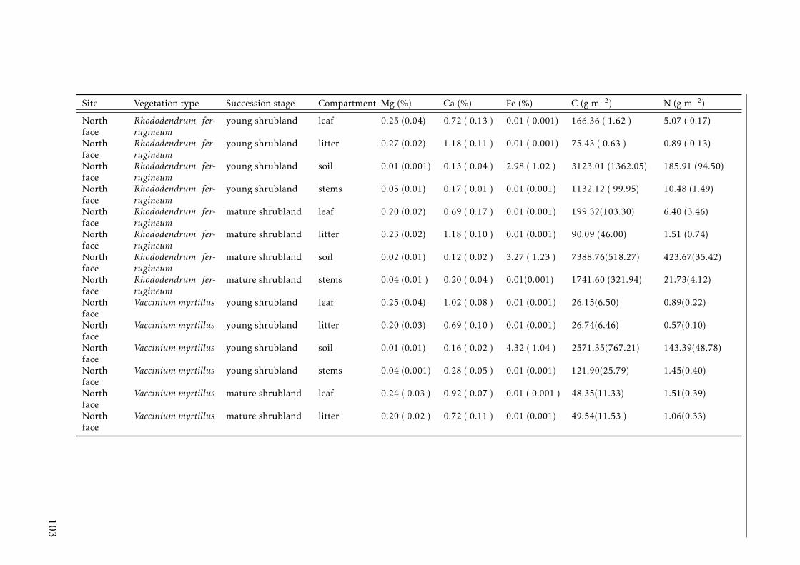
Site Vegetation type Succession stage Compartment Mg (%) Ca (%) Fe (%) C (g m−2) N (g m−2)
Northface
Rhododendrum fer-rugineum
young shrubland leaf 0.25 (0.04) 0.72 ( 0.13 ) 0.01 ( 0.001) 166.36 ( 1.62 ) 5.07 ( 0.17)
Northface
Rhododendrum fer-rugineum
young shrubland litter 0.27 (0.02) 1.18 ( 0.11 ) 0.01 ( 0.001) 75.43 ( 0.63 ) 0.89 ( 0.13)
Northface
Rhododendrum fer-rugineum
young shrubland soil 0.01 (0.001) 0.13 ( 0.04 ) 2.98 ( 1.02 ) 3123.01 (1362.05) 185.91 (94.50)
Northface
Rhododendrum fer-rugineum
young shrubland stems 0.05 (0.01) 0.17 ( 0.01 ) 0.01 (0.001) 1132.12 ( 99.95) 10.48 (1.49)
Northface
Rhododendrum fer-rugineum
mature shrubland leaf 0.20 (0.02) 0.69 ( 0.17 ) 0.01 (0.001) 199.32(103.30) 6.40 (3.46)
Northface
Rhododendrum fer-rugineum
mature shrubland litter 0.23 (0.02) 1.18 ( 0.10 ) 0.01 (0.001) 90.09 (46.00) 1.51 (0.74)
Northface
Rhododendrum fer-rugineum
mature shrubland soil 0.02 (0.01) 0.12 ( 0.02 ) 3.27 ( 1.23 ) 7388.76(518.27) 423.67(35.42)
Northface
Rhododendrum fer-rugineum
mature shrubland stems 0.04 (0.01 ) 0.20 ( 0.04 ) 0.01(0.001) 1741.60 (321.94) 21.73(4.12)
Northface
Vaccinium myrtillus young shrubland leaf 0.25 (0.04) 1.02 ( 0.08 ) 0.01 (0.001) 26.15(6.50) 0.89(0.22)
Northface
Vaccinium myrtillus young shrubland litter 0.20 (0.03) 0.69 ( 0.10 ) 0.01 (0.001) 26.74(6.46) 0.57(0.10)
Northface
Vaccinium myrtillus young shrubland soil 0.01 (0.01) 0.16 ( 0.02 ) 4.32 ( 1.04 ) 2571.35(767.21) 143.39(48.78)
Northface
Vaccinium myrtillus young shrubland stems 0.04 (0.001) 0.28 ( 0.05 ) 0.01 (0.001) 121.90(25.79) 1.45(0.40)
Northface
Vaccinium myrtillus mature shrubland leaf 0.24 ( 0.03 ) 0.92 ( 0.07 ) 0.01 ( 0.001 ) 48.35(11.33) 1.51(0.39)
Northface
Vaccinium myrtillus mature shrubland litter 0.20 ( 0.02 ) 0.72 ( 0.11 ) 0.01 (0.001) 49.54(11.53 ) 1.06(0.33)
103
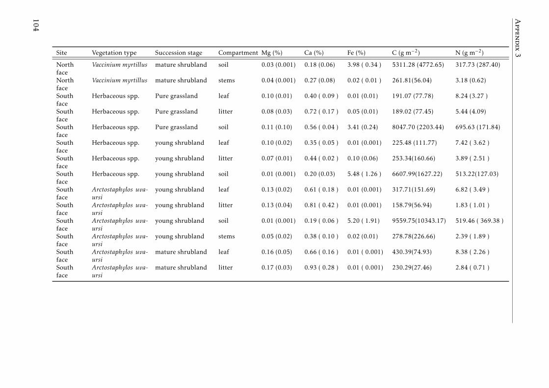
Appendix3Site Vegetation type Succession stage Compartment Mg (%) Ca (%) Fe (%) C (g m−2) N (g m−2)
Northface
Vaccinium myrtillus mature shrubland soil 0.03 (0.001) 0.18 (0.06) 3.98 ( 0.34 ) 5311.28 (4772.65) 317.73 (287.40)
Northface
Vaccinium myrtillus mature shrubland stems 0.04 (0.001) 0.27 (0.08) 0.02 ( 0.01 ) 261.81(56.04) 3.18 (0.62)
Southface
Herbaceous spp. Pure grassland leaf 0.10 (0.01) 0.40 ( 0.09 ) 0.01 (0.01) 191.07 (77.78) 8.24 (3.27 )
Southface
Herbaceous spp. Pure grassland litter 0.08 (0.03) 0.72 ( 0.17 ) 0.05 (0.01) 189.02 (77.45) 5.44 (4.09)
Southface
Herbaceous spp. Pure grassland soil 0.11 (0.10) 0.56 ( 0.04 ) 3.41 (0.24) 8047.70 (2203.44) 695.63 (171.84)
Southface
Herbaceous spp. young shrubland leaf 0.10 (0.02) 0.35 ( 0.05 ) 0.01 (0.001) 225.48 (111.77) 7.42 ( 3.62 )
Southface
Herbaceous spp. young shrubland litter 0.07 (0.01) 0.44 ( 0.02 ) 0.10 (0.06) 253.34(160.66) 3.89 ( 2.51 )
Southface
Herbaceous spp. young shrubland soil 0.01 (0.001) 0.20 (0.03) 5.48 ( 1.26 ) 6607.99(1627.22) 513.22(127.03)
Southface
Arctostaphylos uva-ursi
young shrubland leaf 0.13 (0.02) 0.61 ( 0.18 ) 0.01 (0.001) 317.71(151.69) 6.82 ( 3.49 )
Southface
Arctostaphylos uva-ursi
young shrubland litter 0.13 (0.04) 0.81 ( 0.42 ) 0.01 (0.001) 158.79(56.94) 1.83 ( 1.01 )
Southface
Arctostaphylos uva-ursi
young shrubland soil 0.01 (0.001) 0.19 ( 0.06 ) 5.20 ( 1.91) 9559.75(10343.17) 519.46 ( 369.38 )
Southface
Arctostaphylos uva-ursi
young shrubland stems 0.05 (0.02) 0.38 ( 0.10 ) 0.02 (0.01) 278.78(226.66) 2.39 ( 1.89 )
Southface
Arctostaphylos uva-ursi
mature shrubland leaf 0.16 (0.05) 0.66 ( 0.16 ) 0.01 ( 0.001) 430.39(74.93) 8.38 ( 2.26 )
Southface
Arctostaphylos uva-ursi
mature shrubland litter 0.17 (0.03) 0.93 ( 0.28 ) 0.01 ( 0.001) 230.29(27.46) 2.84 ( 0.71 )
104
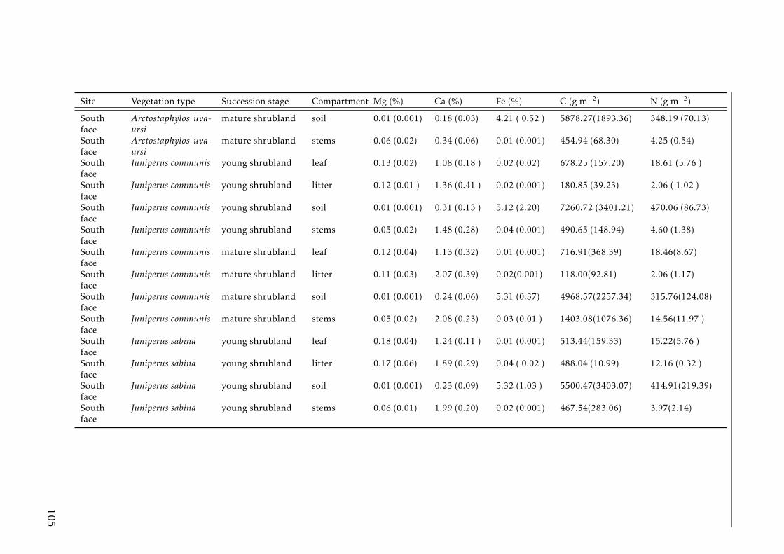
Site Vegetation type Succession stage Compartment Mg (%) Ca (%) Fe (%) C (g m−2) N (g m−2)
Southface
Arctostaphylos uva-ursi
mature shrubland soil 0.01 (0.001) 0.18 (0.03) 4.21 ( 0.52 ) 5878.27(1893.36) 348.19 (70.13)
Southface
Arctostaphylos uva-ursi
mature shrubland stems 0.06 (0.02) 0.34 (0.06) 0.01 (0.001) 454.94 (68.30) 4.25 (0.54)
Southface
Juniperus communis young shrubland leaf 0.13 (0.02) 1.08 (0.18 ) 0.02 (0.02) 678.25 (157.20) 18.61 (5.76 )
Southface
Juniperus communis young shrubland litter 0.12 (0.01 ) 1.36 (0.41 ) 0.02 (0.001) 180.85 (39.23) 2.06 ( 1.02 )
Southface
Juniperus communis young shrubland soil 0.01 (0.001) 0.31 (0.13 ) 5.12 (2.20) 7260.72 (3401.21) 470.06 (86.73)
Southface
Juniperus communis young shrubland stems 0.05 (0.02) 1.48 (0.28) 0.04 (0.001) 490.65 (148.94) 4.60 (1.38)
Southface
Juniperus communis mature shrubland leaf 0.12 (0.04) 1.13 (0.32) 0.01 (0.001) 716.91(368.39) 18.46(8.67)
Southface
Juniperus communis mature shrubland litter 0.11 (0.03) 2.07 (0.39) 0.02(0.001) 118.00(92.81) 2.06 (1.17)
Southface
Juniperus communis mature shrubland soil 0.01 (0.001) 0.24 (0.06) 5.31 (0.37) 4968.57(2257.34) 315.76(124.08)
Southface
Juniperus communis mature shrubland stems 0.05 (0.02) 2.08 (0.23) 0.03 (0.01 ) 1403.08(1076.36) 14.56(11.97 )
Southface
Juniperus sabina young shrubland leaf 0.18 (0.04) 1.24 (0.11 ) 0.01 (0.001) 513.44(159.33) 15.22(5.76 )
Southface
Juniperus sabina young shrubland litter 0.17 (0.06) 1.89 (0.29) 0.04 ( 0.02 ) 488.04 (10.99) 12.16 (0.32 )
Southface
Juniperus sabina young shrubland soil 0.01 (0.001) 0.23 (0.09) 5.32 (1.03 ) 5500.47(3403.07) 414.91(219.39)
Southface
Juniperus sabina young shrubland stems 0.06 (0.01) 1.99 (0.20) 0.02 (0.001) 467.54(283.06) 3.97(2.14)
105
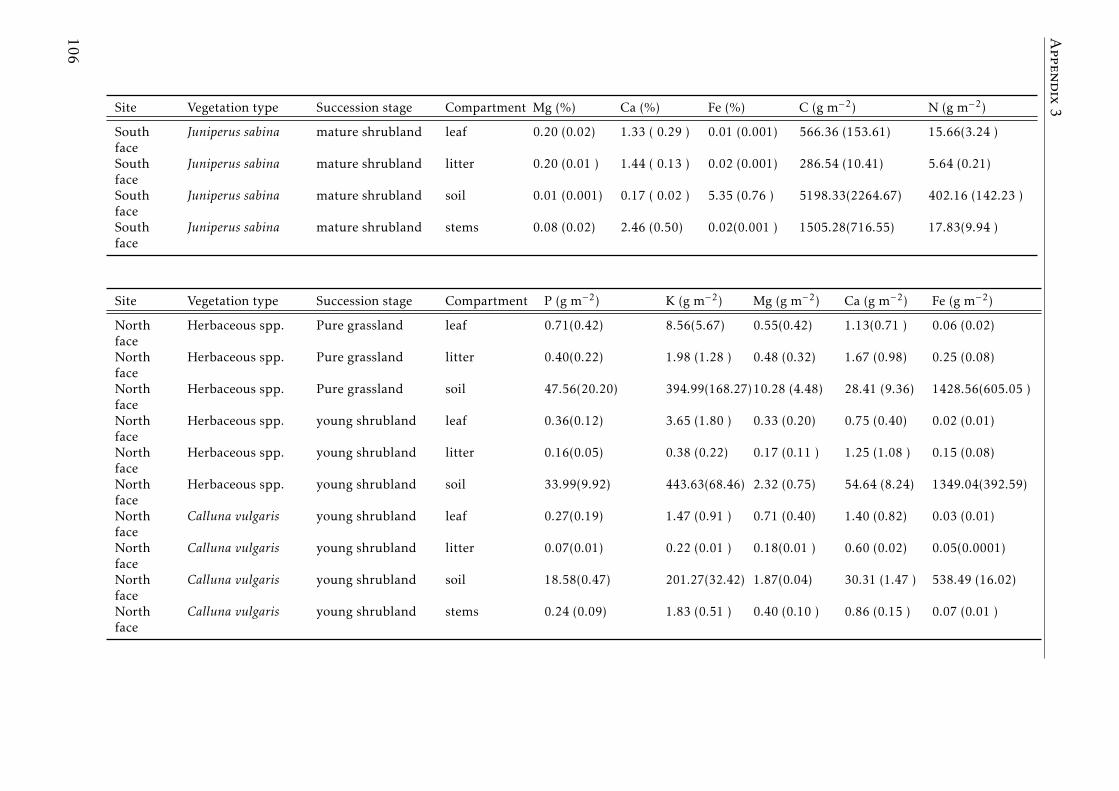
Appendix3Site Vegetation type Succession stage Compartment Mg (%) Ca (%) Fe (%) C (g m−2) N (g m−2)
Southface
Juniperus sabina mature shrubland leaf 0.20 (0.02) 1.33 ( 0.29 ) 0.01 (0.001) 566.36 (153.61) 15.66(3.24 )
Southface
Juniperus sabina mature shrubland litter 0.20 (0.01 ) 1.44 ( 0.13 ) 0.02 (0.001) 286.54 (10.41) 5.64 (0.21)
Southface
Juniperus sabina mature shrubland soil 0.01 (0.001) 0.17 ( 0.02 ) 5.35 (0.76 ) 5198.33(2264.67) 402.16 (142.23 )
Southface
Juniperus sabina mature shrubland stems 0.08 (0.02) 2.46 (0.50) 0.02(0.001 ) 1505.28(716.55) 17.83(9.94 )
Site Vegetation type Succession stage Compartment P (g m−2) K (g m−2) Mg (g m−2) Ca (g m−2) Fe (g m−2)
Northface
Herbaceous spp. Pure grassland leaf 0.71(0.42) 8.56(5.67) 0.55(0.42) 1.13(0.71 ) 0.06 (0.02)
Northface
Herbaceous spp. Pure grassland litter 0.40(0.22) 1.98 (1.28 ) 0.48 (0.32) 1.67 (0.98) 0.25 (0.08)
Northface
Herbaceous spp. Pure grassland soil 47.56(20.20) 394.99(168.27)10.28 (4.48) 28.41 (9.36) 1428.56(605.05 )
Northface
Herbaceous spp. young shrubland leaf 0.36(0.12) 3.65 (1.80 ) 0.33 (0.20) 0.75 (0.40) 0.02 (0.01)
Northface
Herbaceous spp. young shrubland litter 0.16(0.05) 0.38 (0.22) 0.17 (0.11 ) 1.25 (1.08 ) 0.15 (0.08)
Northface
Herbaceous spp. young shrubland soil 33.99(9.92) 443.63(68.46) 2.32 (0.75) 54.64 (8.24) 1349.04(392.59)
Northface
Calluna vulgaris young shrubland leaf 0.27(0.19) 1.47 (0.91 ) 0.71 (0.40) 1.40 (0.82) 0.03 (0.01)
Northface
Calluna vulgaris young shrubland litter 0.07(0.01) 0.22 (0.01 ) 0.18(0.01 ) 0.60 (0.02) 0.05(0.0001)
Northface
Calluna vulgaris young shrubland soil 18.58(0.47) 201.27(32.42) 1.87(0.04) 30.31 (1.47 ) 538.49 (16.02)
Northface
Calluna vulgaris young shrubland stems 0.24 (0.09) 1.83 (0.51 ) 0.40 (0.10 ) 0.86 (0.15 ) 0.07 (0.01 )
106
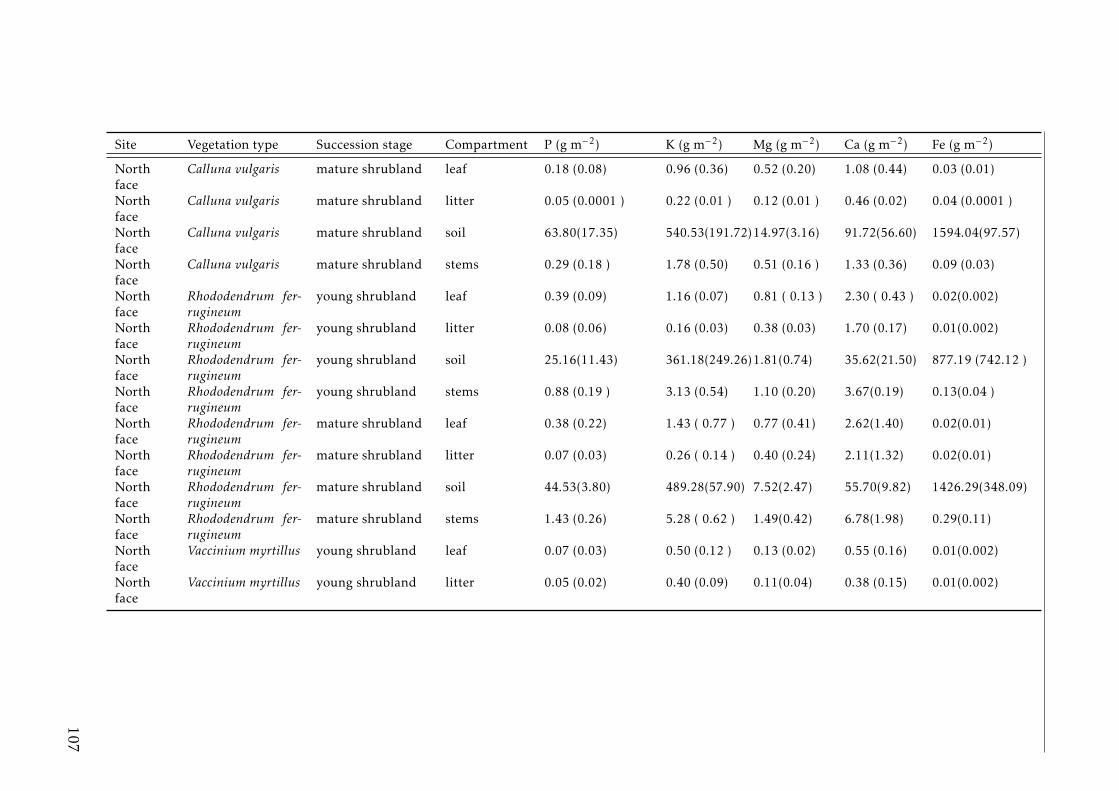
Site Vegetation type Succession stage Compartment P (g m−2) K (g m−2) Mg (g m−2) Ca (g m−2) Fe (g m−2)
Northface
Calluna vulgaris mature shrubland leaf 0.18 (0.08) 0.96 (0.36) 0.52 (0.20) 1.08 (0.44) 0.03 (0.01)
Northface
Calluna vulgaris mature shrubland litter 0.05 (0.0001 ) 0.22 (0.01 ) 0.12 (0.01 ) 0.46 (0.02) 0.04 (0.0001 )
Northface
Calluna vulgaris mature shrubland soil 63.80(17.35) 540.53(191.72)14.97(3.16) 91.72(56.60) 1594.04(97.57)
Northface
Calluna vulgaris mature shrubland stems 0.29 (0.18 ) 1.78 (0.50) 0.51 (0.16 ) 1.33 (0.36) 0.09 (0.03)
Northface
Rhododendrum fer-rugineum
young shrubland leaf 0.39 (0.09) 1.16 (0.07) 0.81 ( 0.13 ) 2.30 ( 0.43 ) 0.02(0.002)
Northface
Rhododendrum fer-rugineum
young shrubland litter 0.08 (0.06) 0.16 (0.03) 0.38 (0.03) 1.70 (0.17) 0.01(0.002)
Northface
Rhododendrum fer-rugineum
young shrubland soil 25.16(11.43) 361.18(249.26)1.81(0.74) 35.62(21.50) 877.19 (742.12 )
Northface
Rhododendrum fer-rugineum
young shrubland stems 0.88 (0.19 ) 3.13 (0.54) 1.10 (0.20) 3.67(0.19) 0.13(0.04 )
Northface
Rhododendrum fer-rugineum
mature shrubland leaf 0.38 (0.22) 1.43 ( 0.77 ) 0.77 (0.41) 2.62(1.40) 0.02(0.01)
Northface
Rhododendrum fer-rugineum
mature shrubland litter 0.07 (0.03) 0.26 ( 0.14 ) 0.40 (0.24) 2.11(1.32) 0.02(0.01)
Northface
Rhododendrum fer-rugineum
mature shrubland soil 44.53(3.80) 489.28(57.90) 7.52(2.47) 55.70(9.82) 1426.29(348.09)
Northface
Rhododendrum fer-rugineum
mature shrubland stems 1.43 (0.26) 5.28 ( 0.62 ) 1.49(0.42) 6.78(1.98) 0.29(0.11)
Northface
Vaccinium myrtillus young shrubland leaf 0.07 (0.03) 0.50 (0.12 ) 0.13 (0.02) 0.55 (0.16) 0.01(0.002)
Northface
Vaccinium myrtillus young shrubland litter 0.05 (0.02) 0.40 (0.09) 0.11(0.04) 0.38 (0.15) 0.01(0.002)
107
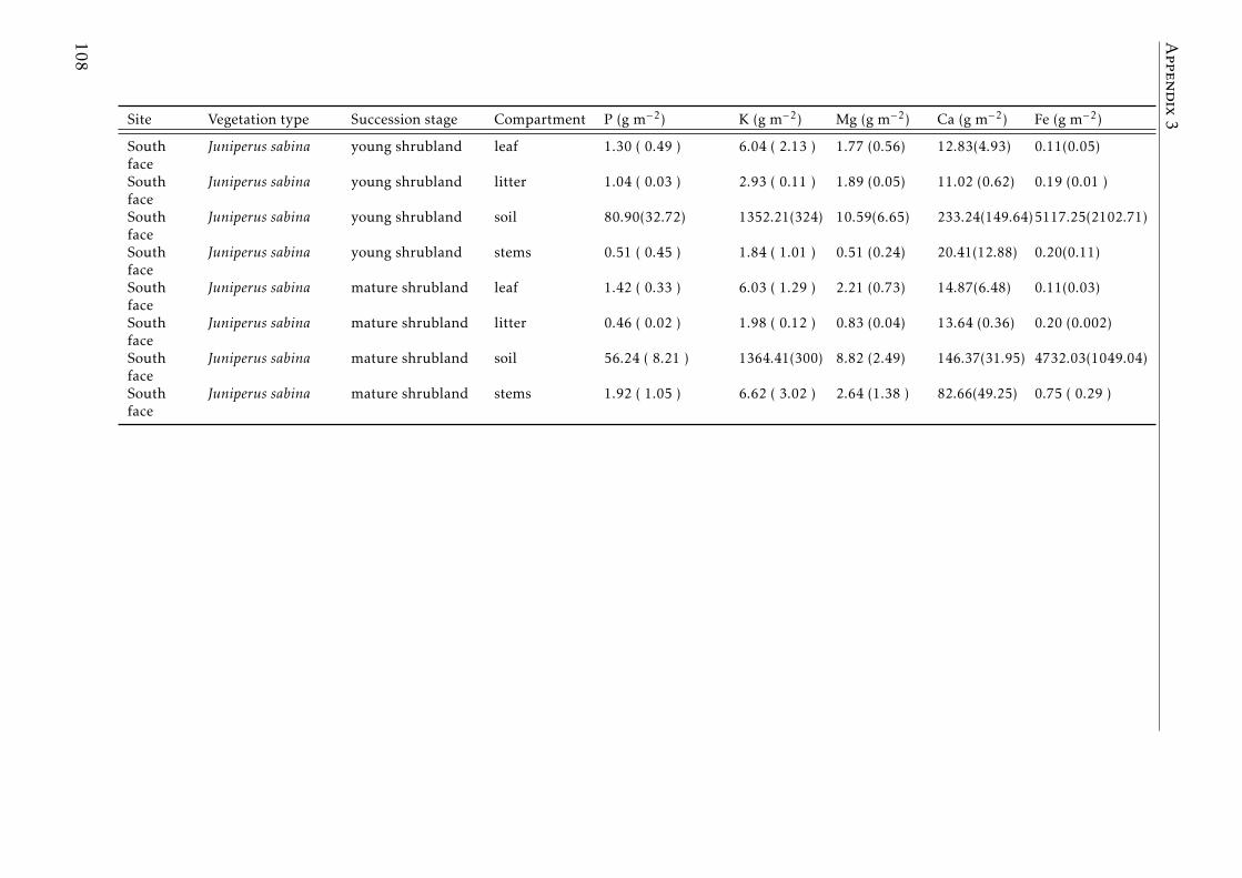
Appendix3Site Vegetation type Succession stage Compartment P (g m−2) K (g m−2) Mg (g m−2) Ca (g m−2) Fe (g m−2)
Southface
Juniperus sabina young shrubland leaf 1.30 ( 0.49 ) 6.04 ( 2.13 ) 1.77 (0.56) 12.83(4.93) 0.11(0.05)
Southface
Juniperus sabina young shrubland litter 1.04 ( 0.03 ) 2.93 ( 0.11 ) 1.89 (0.05) 11.02 (0.62) 0.19 (0.01 )
Southface
Juniperus sabina young shrubland soil 80.90(32.72) 1352.21(324) 10.59(6.65) 233.24(149.64)5117.25(2102.71)
Southface
Juniperus sabina young shrubland stems 0.51 ( 0.45 ) 1.84 ( 1.01 ) 0.51 (0.24) 20.41(12.88) 0.20(0.11)
Southface
Juniperus sabina mature shrubland leaf 1.42 ( 0.33 ) 6.03 ( 1.29 ) 2.21 (0.73) 14.87(6.48) 0.11(0.03)
Southface
Juniperus sabina mature shrubland litter 0.46 ( 0.02 ) 1.98 ( 0.12 ) 0.83 (0.04) 13.64 (0.36) 0.20 (0.002)
Southface
Juniperus sabina mature shrubland soil 56.24 ( 8.21 ) 1364.41(300) 8.82 (2.49) 146.37(31.95) 4732.03(1049.04)
Southface
Juniperus sabina mature shrubland stems 1.92 ( 1.05 ) 6.62 ( 3.02 ) 2.64 (1.38 ) 82.66(49.25) 0.75 ( 0.29 )
108
Appendix 4: Chapter - High foliar Kand P resorption efficiencies inold-growth nutrient-poor tropicalforests
109
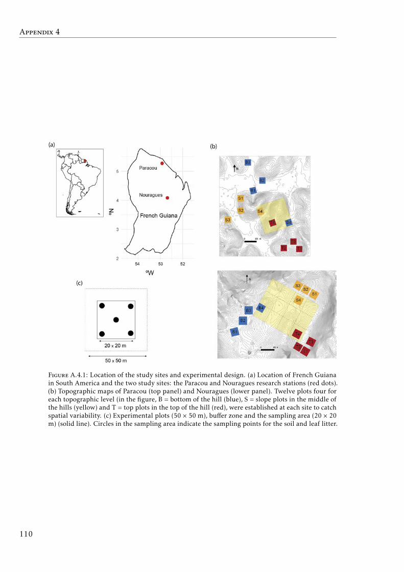
Appendix 4
Figure A.4.1: Location of the study sites and experimental design. (a) Location of French Guianain South America and the two study sites: the Paracou and Nouragues research stations (red dots).(b) Topographic maps of Paracou (top panel) and Nouragues (lower panel). Twelve plots four foreach topographic level (in the figure, B = bottom of the hill (blue), S = slope plots in the middle ofthe hills (yellow) and T = top plots in the top of the hill (red), were established at each site to catchspatial variability. (c) Experimental plots (50 × 50 m), buffer zone and the sampling area (20 × 20m) (solid line). Circles in the sampling area indicate the sampling points for the soil and leaf litter.
110
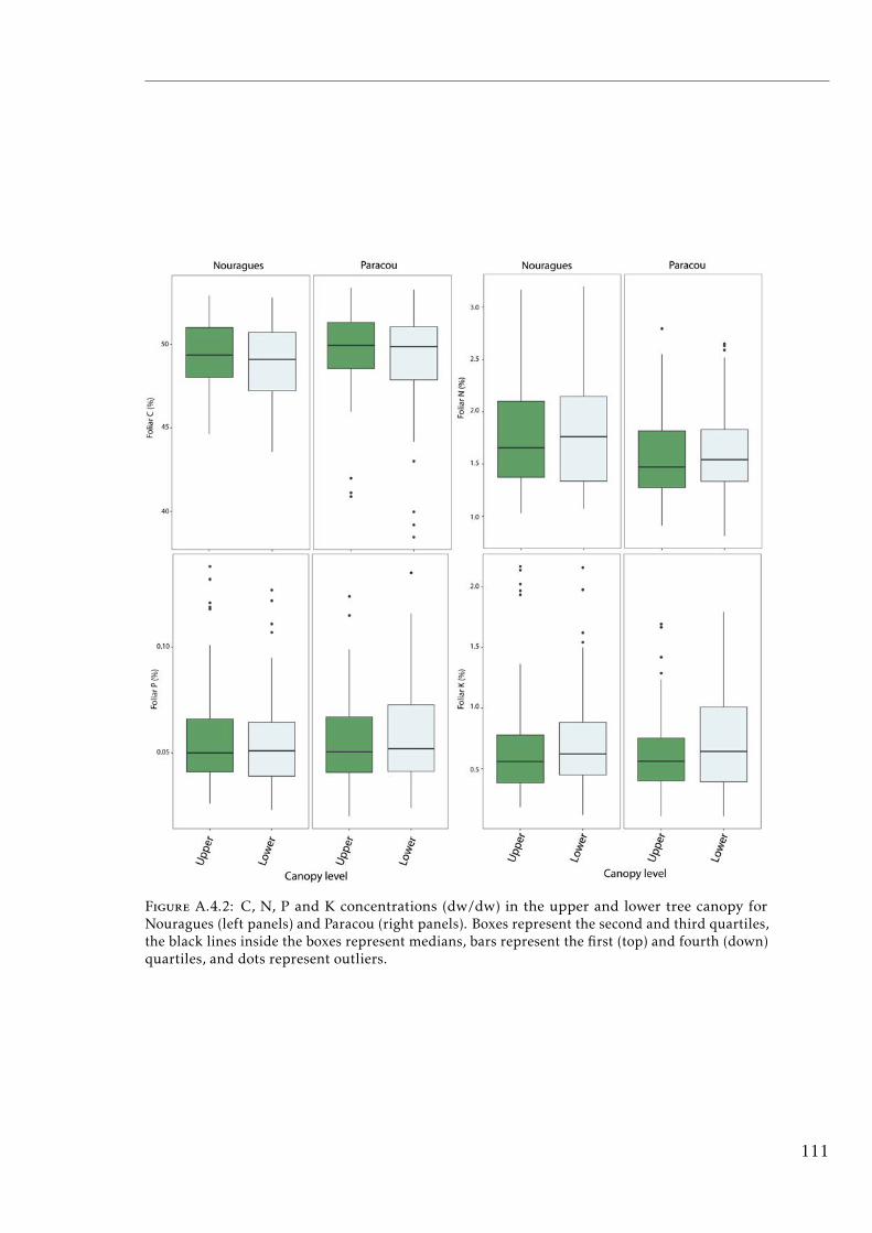
Figure A.4.2: C, N, P and K concentrations (dw/dw) in the upper and lower tree canopy forNouragues (left panels) and Paracou (right panels). Boxes represent the second and third quartiles,the black lines inside the boxes represent medians, bars represent the first (top) and fourth (down)quartiles, and dots represent outliers.
111
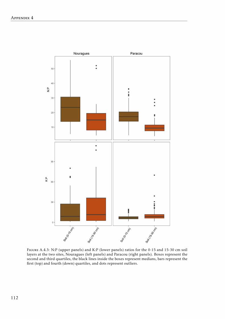
Appendix 4
Figure A.4.3: N:P (upper panels) and K:P (lower panels) ratios for the 0-15 and 15-30 cm soillayers at the two sites, Nouragues (left panels) and Paracou (right panels). Boxes represent thesecond and third quartiles, the black lines inside the boxes represent medians, bars represent thefirst (top) and fourth (down) quartiles, and dots represent outliers.
112
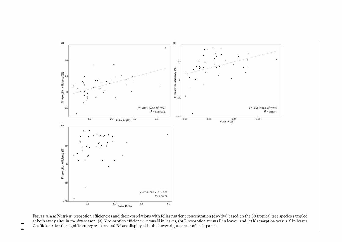
Figure A.4.4: Nutrient resorption efficiencies and their correlations with foliar nutrient concentration (dw/dw) based on the 39 tropical tree species sampledat both study sites in the dry season. (a) N resorption efficiency versus N in leaves, (b) P resorption versus P in leaves, and (c) K resorption versus K in leaves.Coefficients for the significant regressions and R2 are displayed in the lower-right corner of each panel.
113
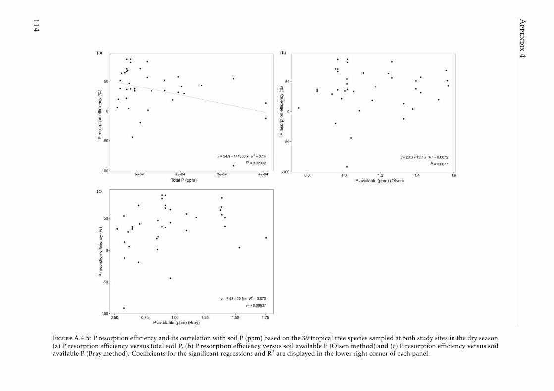
Appendix4
Figure A.4.5: P resorption efficiency and its correlation with soil P (ppm) based on the 39 tropical tree species sampled at both study sites in the dry season.(a) P resorption efficiency versus total soil P, (b) P resorption efficiency versus soil available P (Olsen method) and (c) P resorption efficiency versus soilavailable P (Bray method). Coefficients for the significant regressions and R2 are displayed in the lower-right corner of each panel.
114
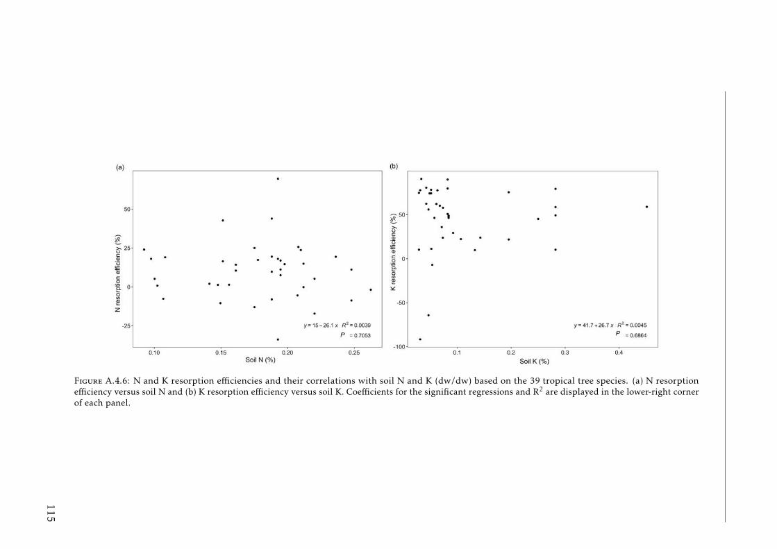
Figure A.4.6: N and K resorption efficiencies and their correlations with soil N and K (dw/dw) based on the 39 tropical tree species. (a) N resorptionefficiency versus soil N and (b) K resorption efficiency versus soil K. Coefficients for the significant regressions and R2 are displayed in the lower-right cornerof each panel.
115
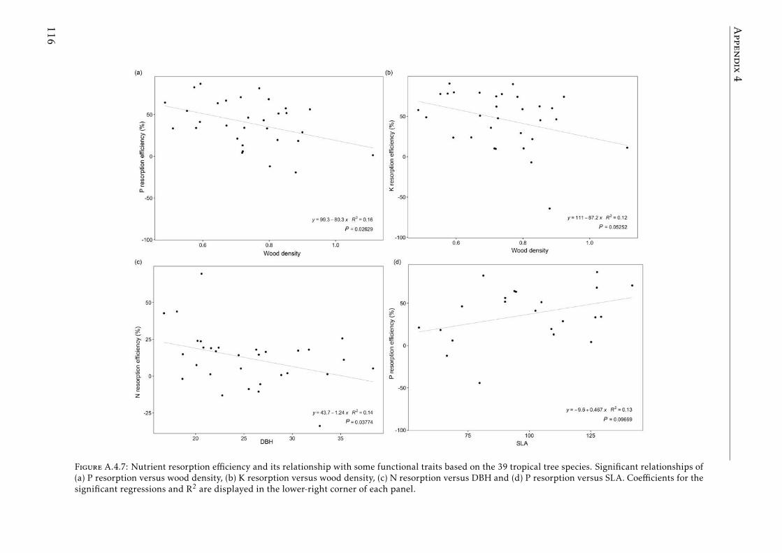
Appendix4
Figure A.4.7: Nutrient resorption efficiency and its relationship with some functional traits based on the 39 tropical tree species. Significant relationships of(a) P resorption versus wood density, (b) K resorption versus wood density, (c) N resorption versus DBH and (d) P resorption versus SLA. Coefficients for thesignificant regressions and R2 are displayed in the lower-right corner of each panel.
116
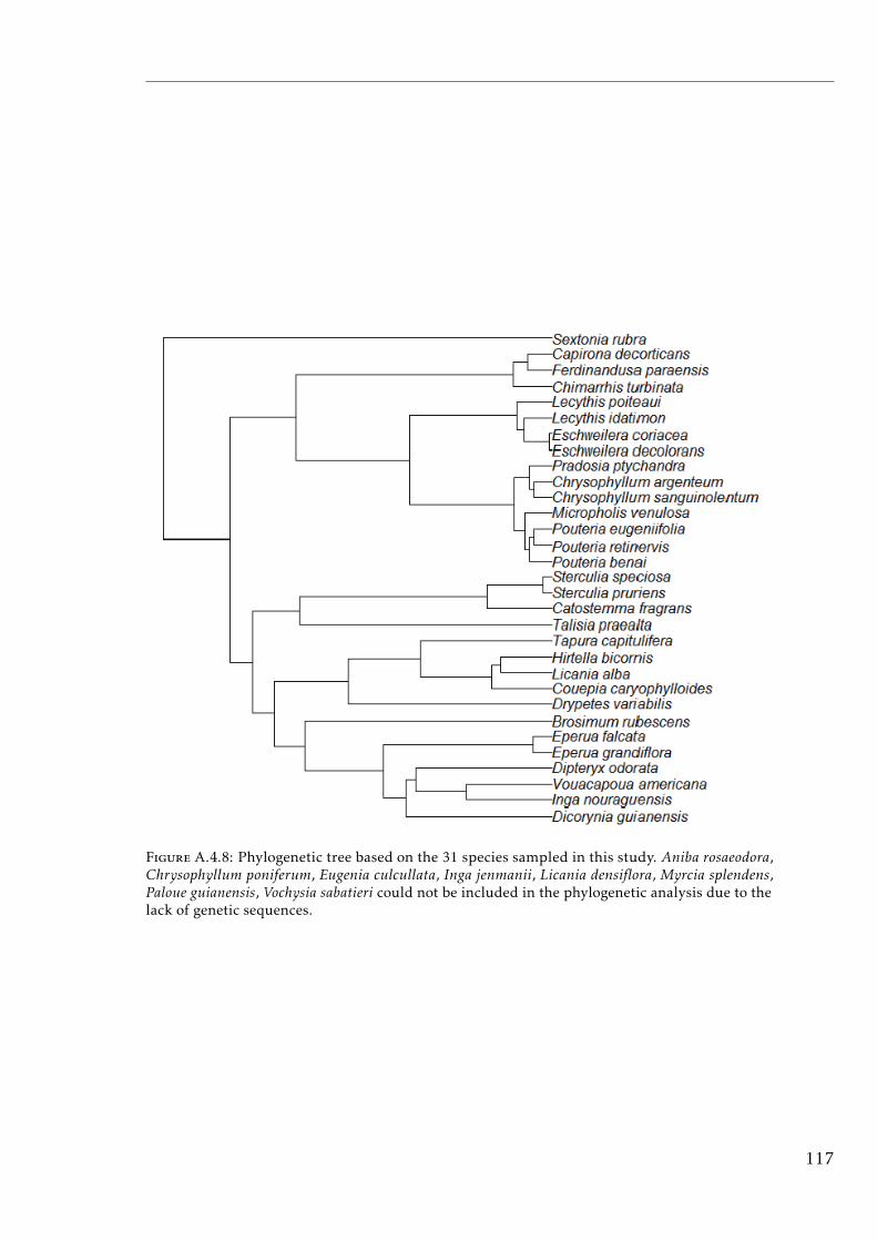
Figure A.4.8: Phylogenetic tree based on the 31 species sampled in this study. Aniba rosaeodora,Chrysophyllum poniferum, Eugenia culcullata, Inga jenmanii, Licania densiflora, Myrcia splendens,Paloue guianensis, Vochysia sabatieri could not be included in the phylogenetic analysis due to thelack of genetic sequences.
117
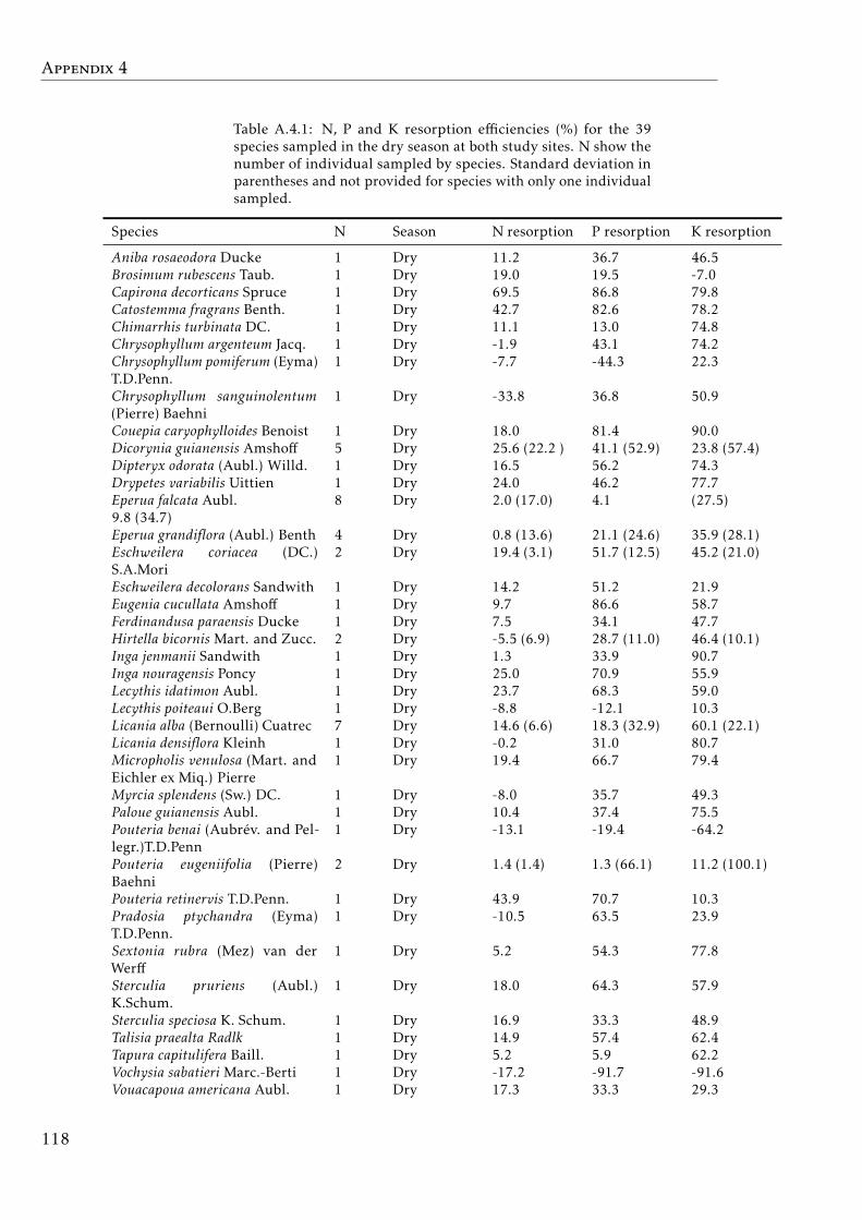
Appendix 4
Table A.4.1: N, P and K resorption efficiencies (%) for the 39species sampled in the dry season at both study sites. N show thenumber of individual sampled by species. Standard deviation inparentheses and not provided for species with only one individualsampled.
Species N Season N resorption P resorption K resorption
Aniba rosaeodora Ducke 1 Dry 11.2 36.7 46.5Brosimum rubescens Taub. 1 Dry 19.0 19.5 -7.0Capirona decorticans Spruce 1 Dry 69.5 86.8 79.8Catostemma fragrans Benth. 1 Dry 42.7 82.6 78.2Chimarrhis turbinata DC. 1 Dry 11.1 13.0 74.8Chrysophyllum argenteum Jacq. 1 Dry -1.9 43.1 74.2Chrysophyllum pomiferum (Eyma)T.D.Penn.
1 Dry -7.7 -44.3 22.3
Chrysophyllum sanguinolentum(Pierre) Baehni
1 Dry -33.8 36.8 50.9
Couepia caryophylloides Benoist 1 Dry 18.0 81.4 90.0Dicorynia guianensis Amshoff 5 Dry 25.6 (22.2 ) 41.1 (52.9) 23.8 (57.4)Dipteryx odorata (Aubl.) Willd. 1 Dry 16.5 56.2 74.3Drypetes variabilis Uittien 1 Dry 24.0 46.2 77.7Eperua falcata Aubl. 8 Dry 2.0 (17.0) 4.1 (27.5)9.8 (34.7)Eperua grandiflora (Aubl.) Benth 4 Dry 0.8 (13.6) 21.1 (24.6) 35.9 (28.1)Eschweilera coriacea (DC.)S.A.Mori
2 Dry 19.4 (3.1) 51.7 (12.5) 45.2 (21.0)
Eschweilera decolorans Sandwith 1 Dry 14.2 51.2 21.9Eugenia cucullata Amshoff 1 Dry 9.7 86.6 58.7Ferdinandusa paraensis Ducke 1 Dry 7.5 34.1 47.7Hirtella bicornis Mart. and Zucc. 2 Dry -5.5 (6.9) 28.7 (11.0) 46.4 (10.1)Inga jenmanii Sandwith 1 Dry 1.3 33.9 90.7Inga nouragensis Poncy 1 Dry 25.0 70.9 55.9Lecythis idatimon Aubl. 1 Dry 23.7 68.3 59.0Lecythis poiteaui O.Berg 1 Dry -8.8 -12.1 10.3Licania alba (Bernoulli) Cuatrec 7 Dry 14.6 (6.6) 18.3 (32.9) 60.1 (22.1)Licania densiflora Kleinh 1 Dry -0.2 31.0 80.7Micropholis venulosa (Mart. andEichler ex Miq.) Pierre
1 Dry 19.4 66.7 79.4
Myrcia splendens (Sw.) DC. 1 Dry -8.0 35.7 49.3Paloue guianensis Aubl. 1 Dry 10.4 37.4 75.5Pouteria benai (Aubrev. and Pel-legr.)T.D.Penn
1 Dry -13.1 -19.4 -64.2
Pouteria eugeniifolia (Pierre)Baehni
2 Dry 1.4 (1.4) 1.3 (66.1) 11.2 (100.1)
Pouteria retinervis T.D.Penn. 1 Dry 43.9 70.7 10.3Pradosia ptychandra (Eyma)T.D.Penn.
1 Dry -10.5 63.5 23.9
Sextonia rubra (Mez) van derWerff
1 Dry 5.2 54.3 77.8
Sterculia pruriens (Aubl.)K.Schum.
1 Dry 18.0 64.3 57.9
Sterculia speciosa K. Schum. 1 Dry 16.9 33.3 48.9Talisia praealta Radlk 1 Dry 14.9 57.4 62.4Tapura capitulifera Baill. 1 Dry 5.2 5.9 62.2Vochysia sabatieri Marc.-Berti 1 Dry -17.2 -91.7 -91.6Vouacapoua americana Aubl. 1 Dry 17.3 33.3 29.3
118
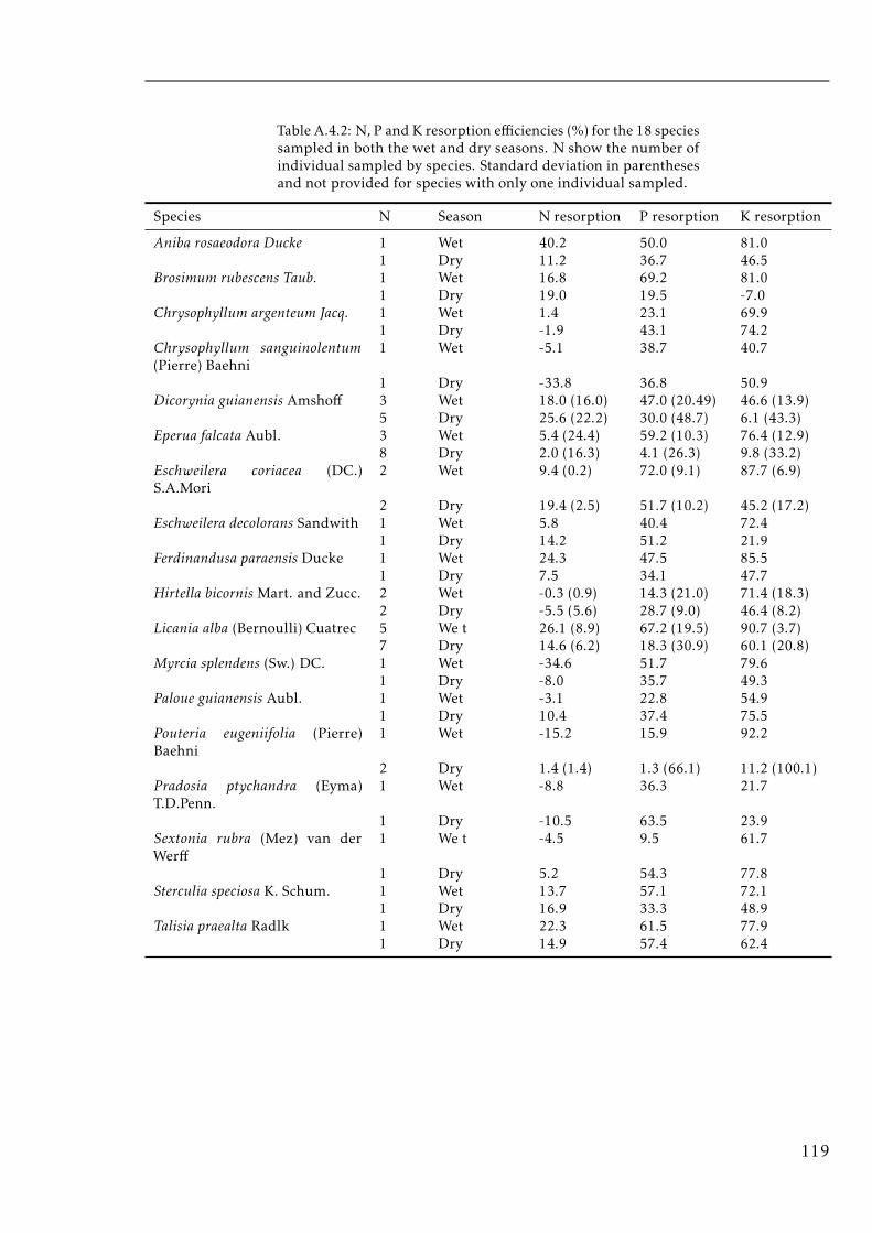
Table A.4.2: N, P and K resorption efficiencies (%) for the 18 speciessampled in both the wet and dry seasons. N show the number ofindividual sampled by species. Standard deviation in parenthesesand not provided for species with only one individual sampled.
Species N Season N resorption P resorption K resorption
Aniba rosaeodora Ducke 1 Wet 40.2 50.0 81.01 Dry 11.2 36.7 46.5
Brosimum rubescens Taub. 1 Wet 16.8 69.2 81.01 Dry 19.0 19.5 -7.0
Chrysophyllum argenteum Jacq. 1 Wet 1.4 23.1 69.91 Dry -1.9 43.1 74.2
Chrysophyllum sanguinolentum(Pierre) Baehni
1 Wet -5.1 38.7 40.7
1 Dry -33.8 36.8 50.9Dicorynia guianensis Amshoff 3 Wet 18.0 (16.0) 47.0 (20.49) 46.6 (13.9)
5 Dry 25.6 (22.2) 30.0 (48.7) 6.1 (43.3)Eperua falcata Aubl. 3 Wet 5.4 (24.4) 59.2 (10.3) 76.4 (12.9)
8 Dry 2.0 (16.3) 4.1 (26.3) 9.8 (33.2)Eschweilera coriacea (DC.)S.A.Mori
2 Wet 9.4 (0.2) 72.0 (9.1) 87.7 (6.9)
2 Dry 19.4 (2.5) 51.7 (10.2) 45.2 (17.2)Eschweilera decolorans Sandwith 1 Wet 5.8 40.4 72.4
1 Dry 14.2 51.2 21.9Ferdinandusa paraensis Ducke 1 Wet 24.3 47.5 85.5
1 Dry 7.5 34.1 47.7Hirtella bicornis Mart. and Zucc. 2 Wet -0.3 (0.9) 14.3 (21.0) 71.4 (18.3)
2 Dry -5.5 (5.6) 28.7 (9.0) 46.4 (8.2)Licania alba (Bernoulli) Cuatrec 5 We t 26.1 (8.9) 67.2 (19.5) 90.7 (3.7)
7 Dry 14.6 (6.2) 18.3 (30.9) 60.1 (20.8)Myrcia splendens (Sw.) DC. 1 Wet -34.6 51.7 79.6
1 Dry -8.0 35.7 49.3Paloue guianensis Aubl. 1 Wet -3.1 22.8 54.9
1 Dry 10.4 37.4 75.5Pouteria eugeniifolia (Pierre)Baehni
1 Wet -15.2 15.9 92.2
2 Dry 1.4 (1.4) 1.3 (66.1) 11.2 (100.1)Pradosia ptychandra (Eyma)T.D.Penn.
1 Wet -8.8 36.3 21.7
1 Dry -10.5 63.5 23.9Sextonia rubra (Mez) van derWerff
1 We t -4.5 9.5 61.7
1 Dry 5.2 54.3 77.8Sterculia speciosa K. Schum. 1 Wet 13.7 57.1 72.1
1 Dry 16.9 33.3 48.9Talisia praealta Radlk 1 Wet 22.3 61.5 77.9
1 Dry 14.9 57.4 62.4
119
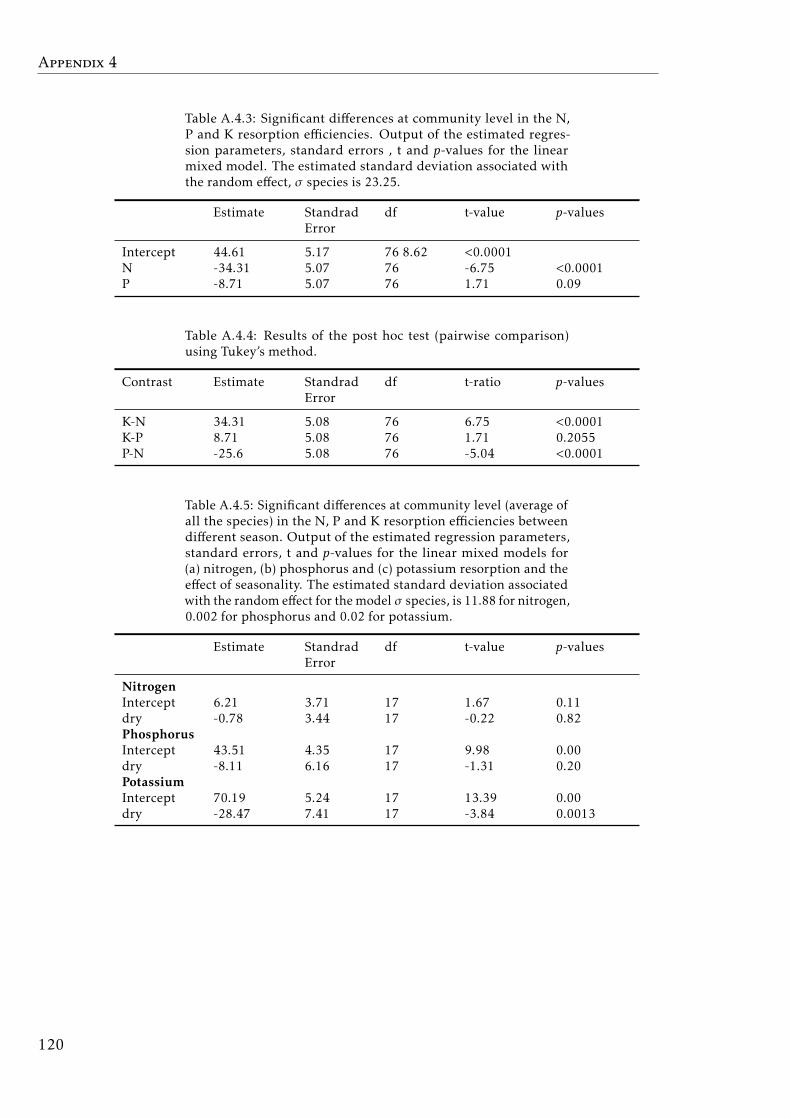
Appendix 4
Table A.4.3: Significant differences at community level in the N,P and K resorption efficiencies. Output of the estimated regres-sion parameters, standard errors , t and p-values for the linearmixed model. The estimated standard deviation associated withthe random effect, σ species is 23.25.
Estimate StandradError
df t-value p-values
Intercept 44.61 5.17 76 8.62 <0.0001N -34.31 5.07 76 -6.75 <0.0001P -8.71 5.07 76 1.71 0.09
Table A.4.4: Results of the post hoc test (pairwise comparison)using Tukey’s method.
Contrast Estimate StandradError
df t-ratio p-values
K-N 34.31 5.08 76 6.75 <0.0001K-P 8.71 5.08 76 1.71 0.2055P-N -25.6 5.08 76 -5.04 <0.0001
Table A.4.5: Significant differences at community level (average ofall the species) in the N, P and K resorption efficiencies betweendifferent season. Output of the estimated regression parameters,standard errors, t and p-values for the linear mixed models for(a) nitrogen, (b) phosphorus and (c) potassium resorption and theeffect of seasonality. The estimated standard deviation associatedwith the random effect for the model σ species, is 11.88 for nitrogen,0.002 for phosphorus and 0.02 for potassium.
Estimate StandradError
df t-value p-values
NitrogenIntercept 6.21 3.71 17 1.67 0.11dry -0.78 3.44 17 -0.22 0.82PhosphorusIntercept 43.51 4.35 17 9.98 0.00dry -8.11 6.16 17 -1.31 0.20PotassiumIntercept 70.19 5.24 17 13.39 0.00dry -28.47 7.41 17 -3.84 0.0013
120
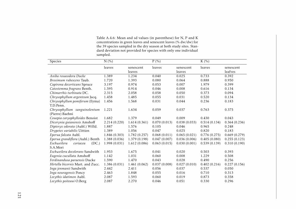
Table A.4.6: Mean and sd values (in parenthese) for N, P and Kconcentrations in green leaves and senescent leaves (% dw/dw) forthe 39 species sampled in the dry season at both study sites. Stan-dard deviation not provided for species with only one individualsampled.
Species N (%) P (%) K (%)
leaves senescentleaves
leaves senescentleaves
leaves senescentleafves
Aniba rosaeodora Ducke 1.389 1.234 0.040 0.025 0.733 0.392Brosimum rubescens Taub. 1.720 1.393 0.080 0.064 0.888 0.950Capirona decorticans Spruce 3.197 0.974 0.053 0.007 1.979 0.399Catostemma fragrans Benth. 1.595 0.914 0.046 0.008 0.616 0.134Chimarrhis turbinata DC. 2.315 2.058 0.058 0.050 0.373 0.094Chrysophyllum argenteum Jacq. 1.458 1.485 0.055 0.031 0.520 0.134Chrysophyllum pomiferum (Eyma)T.D.Penn.
1.456 1.568 0.031 0.044 0.236 0.183
Chrysophyllum sanguinolentum(Pierre) Baehni
1.221 1.634 0.059 0.037 0.763 0.375
Couepia caryophylloides Benoist 1.682 1.379 0.049 0.009 0.430 0.043Dicorynia guianensis Amshoff 2.214 (0.220) 1.614 (0.361) 0.070 (0.013) 0.038 (0.033) 0.514 (0.134) 0.364 (0.236)Dipteryx odorata (Aubl.) Willd. 1.887 1.576 0.105 0.046 0.965 0.248Drypetes variabilis Uittien 1.389 1.056 0.047 0.025 0.820 0.183Eperua falcata Aubl. 1.846 (0.303) 1.782 (0.257) 0.068 (0.011) 0.065 (0.021) 0.776 (0.275) 0.669 (0.279)Eperua grandiflora (Aubl.) Benth 1.388 (0.036) 1.379 (0.198) 0.047 (0.007) 0.036 (0.006) 0.405 (0.080) 0.255 (0.123)Eschweilera coriacea (DC.)S.A.Mori
1.998 (0.031) 1.612 (0.086) 0.063 (0.015) 0.030 (0.001) 0.539 (0.139) 0.310 (0.190)
Eschweilera decolorans Sandwith 1.953 1.675 0.041 0.020 0.503 0.393Eugenia cucullata Amshoff 1.142 1.031 0.060 0.008 1.229 0.508Ferdinandusa paraensis Ducke 1.590 1.470 0.043 0.028 0.490 0.256Hirtella bicornis Mart. and Zucc. 1.386 (0.031) 1.461 (0.062) 0.037 (0.008) 0.027 (0.010) 0.402 (0.216) 0.227 (0.156)Inga jenmanii Sandwith 2.442 2.411 0.056 0.037 0.537 0.050Inga nouragensis Poncy 2.463 1.848 0.055 0.016 0.710 0.313Lecythis idatimon Aubl. 2.087 1.593 0.060 0.019 0.873 0.358Lecythis poiteaui O.Berg 2.087 2.270 0.046 0.051 0.330 0.296
121
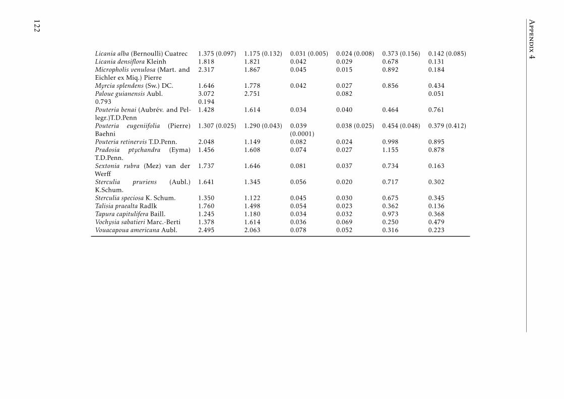
Appendix4Licania alba (Bernoulli) Cuatrec 1.375 (0.097) 1.175 (0.132) 0.031 (0.005) 0.024 (0.008) 0.373 (0.156) 0.142 (0.085)
Licania densiflora Kleinh 1.818 1.821 0.042 0.029 0.678 0.131Micropholis venulosa (Mart. andEichler ex Miq.) Pierre
2.317 1.867 0.045 0.015 0.892 0.184
Myrcia splendens (Sw.) DC. 1.646 1.778 0.042 0.027 0.856 0.434Paloue guianensis Aubl. 3.072 2.751 0.082 0.0510.793 0.194Pouteria benai (Aubrev. and Pel-legr.)T.D.Penn
1.428 1.614 0.034 0.040 0.464 0.761
Pouteria eugeniifolia (Pierre)Baehni
1.307 (0.025) 1.290 (0.043) 0.039(0.0001)
0.038 (0.025) 0.454 (0.048) 0.379 (0.412)
Pouteria retinervis T.D.Penn. 2.048 1.149 0.082 0.024 0.998 0.895Pradosia ptychandra (Eyma)T.D.Penn.
1.456 1.608 0.074 0.027 1.155 0.878
Sextonia rubra (Mez) van derWerff
1.737 1.646 0.081 0.037 0.734 0.163
Sterculia pruriens (Aubl.)K.Schum.
1.641 1.345 0.056 0.020 0.717 0.302
Sterculia speciosa K. Schum. 1.350 1.122 0.045 0.030 0.675 0.345Talisia praealta Radlk 1.760 1.498 0.054 0.023 0.362 0.136Tapura capitulifera Baill. 1.245 1.180 0.034 0.032 0.973 0.368Vochysia sabatieri Marc.-Berti 1.378 1.614 0.036 0.069 0.250 0.479Vouacapoua americana Aubl. 2.495 2.063 0.078 0.052 0.316 0.223
122
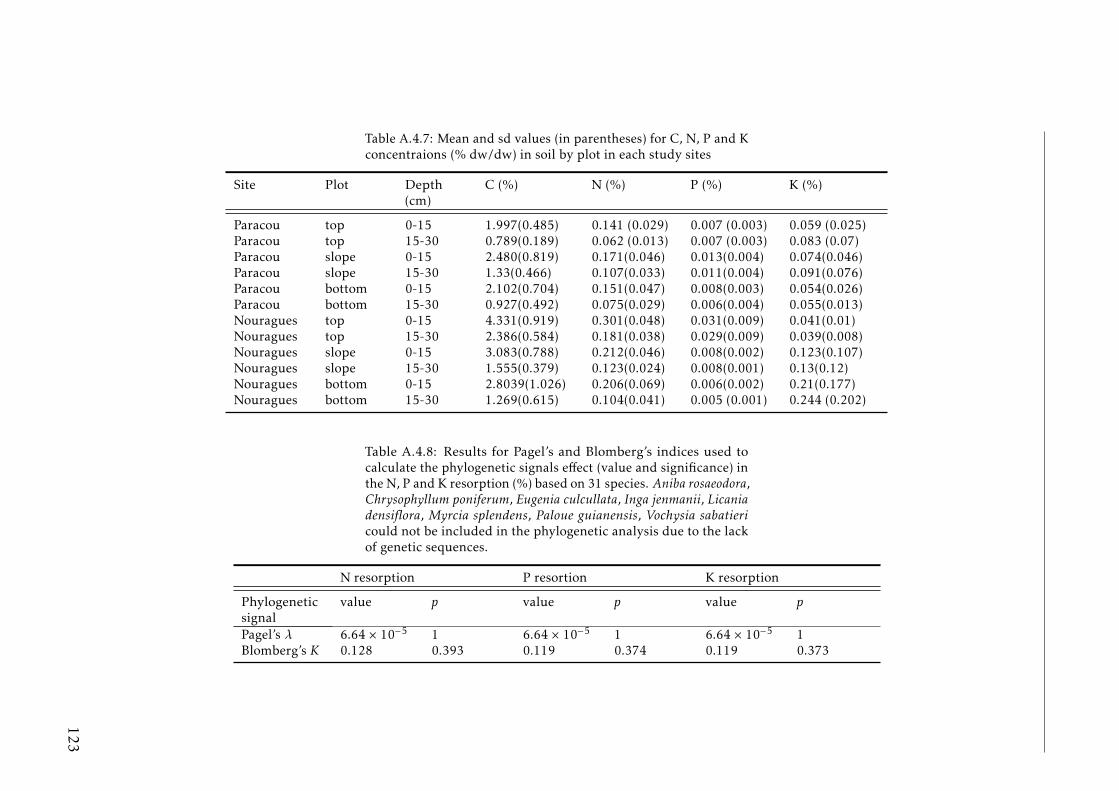
Table A.4.7: Mean and sd values (in parentheses) for C, N, P and Kconcentraions (% dw/dw) in soil by plot in each study sites
Site Plot Depth(cm)
C (%) N (%) P (%) K (%)
Paracou top 0-15 1.997(0.485) 0.141 (0.029) 0.007 (0.003) 0.059 (0.025)Paracou top 15-30 0.789(0.189) 0.062 (0.013) 0.007 (0.003) 0.083 (0.07)Paracou slope 0-15 2.480(0.819) 0.171(0.046) 0.013(0.004) 0.074(0.046)Paracou slope 15-30 1.33(0.466) 0.107(0.033) 0.011(0.004) 0.091(0.076)Paracou bottom 0-15 2.102(0.704) 0.151(0.047) 0.008(0.003) 0.054(0.026)Paracou bottom 15-30 0.927(0.492) 0.075(0.029) 0.006(0.004) 0.055(0.013)Nouragues top 0-15 4.331(0.919) 0.301(0.048) 0.031(0.009) 0.041(0.01)Nouragues top 15-30 2.386(0.584) 0.181(0.038) 0.029(0.009) 0.039(0.008)Nouragues slope 0-15 3.083(0.788) 0.212(0.046) 0.008(0.002) 0.123(0.107)Nouragues slope 15-30 1.555(0.379) 0.123(0.024) 0.008(0.001) 0.13(0.12)Nouragues bottom 0-15 2.8039(1.026) 0.206(0.069) 0.006(0.002) 0.21(0.177)Nouragues bottom 15-30 1.269(0.615) 0.104(0.041) 0.005 (0.001) 0.244 (0.202)
Table A.4.8: Results for Pagel’s and Blomberg’s indices used tocalculate the phylogenetic signals effect (value and significance) inthe N, P and K resorption (%) based on 31 species. Aniba rosaeodora,Chrysophyllum poniferum, Eugenia culcullata, Inga jenmanii, Licaniadensiflora, Myrcia splendens, Paloue guianensis, Vochysia sabatiericould not be included in the phylogenetic analysis due to the lackof genetic sequences.
N resorption P resortion K resorption
Phylogeneticsignal
value p value p value p
Pagel’s λ 6.64 × 10⁻⁵ 1 6.64 × 10⁻⁵ 1 6.64 × 10⁻⁵ 1Blomberg’s K 0.128 0.393 0.119 0.374 0.119 0.373
123

Appendix 4
Deduction of the allometric coefficient (C) for estimating leaf weight basedon diameter at breast height (DBH) from a global data set containing data for2013 tropical trees published by Chave et al. (2014).
log(leaf weight) = log(basalarea) +C (5.1)
basal area =π ×(DBH2 )2
The final model to infer leaf weight from basal area is:
Leaf weight = exp(log(basalarea) +C′) (5.2)
where C’= C + RSE2/2 (Baskerville correction is needed here, because a Gaus-sian error in the log-transformed model is no longer Gaussian when exponential;the error becomes log-normal with a mean of RSE2/2, hence the correction).
The model fit is: C = -4.2569 and Residual Standard Error (RSE) =0.8704, suchthat:
C′ = exp(−4.0153 + 0.8704)(2/2) = 0.02634434 (5.3)
The resulting allometric equation is:
Leaf weight = 0.02634434× basalarea (5.4)
124
Bibliography
Aerts, R. 1996. Nutrient Resorption from Senescing Leaves of Perennials: Arethere General Patterns. Journal of Ecology 84:597–608.
Aerts, R., and F. S. Chapin. 2000. The Mineral Nutrition of Wild Plants Revisited:A Re-evaluation. Advances in Ecological Research 30:55.
Aerts, R., and M. J. Van der Piejl. 1993. A Simple Model to Explain the Dominanceof Low-Productive Perennials in Nutrient-Poor Habitats. Oikos 66:144–147.
Agren, G. I. 2004. The C: N: P stoichiometry of autotrophs - theory and observa-tions. Ecology Letters 7:185–191.
Aguilos, M., C. Stahl, B. Burban, B. Herault, E. Courtois, S. Coste, F. Wagner, etal. 2018. Interannual and Seasonal Variations in Ecosystem Transpiration andWater Use Efficiency in a Tropical Rainforest. Forests 10:14.
Akhmetzhanova, A. A., N. A. Soudzilovskaia, V. G. Onipchenko, W. K. Cornwell,V. A. Agafonov, I. A. Selivanov, and J. H. C. Cornelissen. 2012. A rediscoveredtreasure: mycorrhizal intensity database for 3000 vascular plant species acrossthe former Soviet Union. Ecology 93:689–690.
Ameztegui, A., L. Coll, L. Brotons, and J. M. Ninot. 2016. Land-use legacies ratherthan climate change are driving the recent upward shift of the mountain tree linein the Pyrenees. Global Ecology and Biogeography 25:263–273. Anadon-Rosell,A., S. Palacio, S. Nogues, and J. M. Ninot. 2016. Vaccinium myrtillus stands showsimilar structure and functioning under different scenarios of coexistence at thePyrenean treeline. Plant Ecology 217:1115–1128.
Angulo, M. A., J. M. Ninot, J. Penuelas, J. H. C. Cornelissen, and O. Grau. 2019.Tree Sapling Responses to 10 Years of Experimental Manipulation of Tempera-ture, Nutrient Availability, and Shrub Cover at the Pyrenean Treeline. Frontiersin Plant Science 9:1–13.
Anthelme, F., J.-C. Villaret, and J.-J. Brun. 2007. Shrub encroachment in theAlps gives rise to the convergence of sub-alpine communities on a regional scale.
125
Bibliography
Journal of Vegetation Science 18:355–362.
Baraloto, C., C. E. Timothy Paine, S. Patino, D. Bonal, B. Herault, and J. Chave.2010. Functional trait variation and sampling strategies in species-rich plantcommunities. Functional Ecology 24:208–216.
Baribault, T., R. Kobe, and A. Finley. 2012. Tropical tree growth is correlated withsoil phosphorus, potassium, and calcium, though not for legumes. Dryad DigitalRepository. Ecological Monographs 82:189–203.
Barrio, I. C., C. G. Bueno, L. Nagy, S. Palacio, O. Grau, I. Munilla, M. B. Garcıa, etal. 2013. Alpine Ecology in the Iberian Peninsula: What Do We Know, and WhatDo We Need to Learn? Mountain Research and Development 33:437–442.
Batterman, S. A., J. S. Hall, B. L. Turner, L. O. Hedin, J. K. LaHaela Walter, P.Sheldon, and M. van Breugel. 2018. Phosphatase activity and nitrogen fixationreflect species differences, not nutrient trading or nutrient balance, across tropi-cal rainforest trees. Ecology Letters.
Batterman, S. A., L. O. Hedin, M. Van Breugel, J. Ransijn, D. J. Craven, and J.S. Hall. 2013a. Key role of symbiotic dinitrogen fixation in tropical forest sec-ondary succession. Nature 502:224–227.
Batterman, S. A., N. Wurzburger, and L. O. Hedin. 2013b. Nitrogen and phospho-rus interact to control tropical symbiotic N2 fixation: A test in inga punctata.Journal of Ecology 101:1400–1408.
Boixadera, J., E. Ascaso, C. Herrero, and J. Jaquet. 2014. Els sols de Catalunya Vald’Aran. ICGC-DAAM-Conselh Generau d’Aran.
Bond, W. J. 2010. Do nutrient-poor soils inhibit development of forests? A nutri-ent stock analysis. Plant and Soil 334:47–60.
Bongers, F., P. Charles-Dominique, P. M. Forget, and M. Thery, eds. 2001. Nouragues:dynamics and plant-animal interactions in a neotropical rainforest.
Brant, A. N., and H. Y. H. Chen. 2015. Patterns and Mechanisms of NutrientResorption in Plants. Critical Reviews in Plant Sciences 34:471–486.
Bruijnzeel, L. A. 1991. Nutrient input—output budgets of tropical forest ecosys-tems: A review. Journal of Tropical Ecology 7:1–24.
Bucking, H., E. Liepold, and P. Ambilwade. 2012. The Role of the MycorrhizalSymbiosis in Nutrient Uptake of Plants and the Regulatory Mechanisms Under-lying These Transport Processes. Plant Science. INTECH Open Access Publisher.
126
Cakmak, I. 2005. The role of potassium in alleviating detrimental effects of abioticstresses in plants. Pages 521–530 inJournal of Plant Nutrition and Soil Science(Vol. 168). WILEY-VCH Verlag.
Carreras, J., A. Carrillo, X. Font, J. M. Ninot, and J. Vigo. 1983. Els prats del’alianca Xerobromion als Pirineus Catalans. Collectanea Botanica 14:151–209.
Catalan, J., J. M. Ninot, and M. M. Aniz. 2017. High Mountain Conservation in aChanging World. (J. Catalan, J. M. Ninot, M. M. Aniz, eds.) (1st ed., Vol. 62).Cham.
Chapin, F. S. 1980. The Mineral Nutrition of Wild Plants. Annual Review ofEcology and Systematics 11:233–260. Chapin, F. S., and C. Korner. 1994. Arcticand alpine biodiversity: patterns, causes and ecosystem consequences. Tree9:45–47.
Chapin, F. S., B. H. Walker, R. J. Hobbs, D. U. Hooper, J. H. Lawton, O. E. Sala,and D. Tilman. 1997. Biotic control over the funtioning of ecosystems. Science277:500–504.
Chave, J., D. Coomes, S. Jansen, S. L. Lewis, N. G. Swenson, and A. E. Zanne. 2009.Towards a worldwide wood economics spectrum. Ecology Letters 12:351–366.
Chave, J., M. Mechain-Rejou, A. Burquez, E. Chidumayo, M. Colgan, W. B. C.Delitti, A. Duque, et al. 2014. Improved allometric models to estimate theaboveground biomass of tropical trees. Global Change Biology 20:3177–3190.
Condron, L. M., B. M. Spears, P. M. Haygarth, B. L. Turner, and A. E. Richardson.2013. Role of legacy phosphorus in improving global phosphorus-use efficiency.Environmental Development 8:147–148.
Courtois, E. A., C. Stahl, J. Van den Berge, L. Brechet, L. Van Langenhove, A.Richter, I. Urbina, et al. 2018. Spatial Variation of Soil CO2, CH4 and N2OFluxes Across Topographical Positions in Tropical Forests of the Guiana Shield.Ecosystems.
Craine, J. M., A. J. Elmore, M. P. M. Aidar, M. Bustamante, T. E. Dawson, E. A.Hobbie, A. Kahmen, et al. 2009a. Global patterns of foliar nitrogen isotopes andtheir relationships with climate, mycorrhizal fungi, foliar nutrient concentra-tions, and nitrogen availability. The New phytologist 183:980–92.
Cross, W. F., J. P. Benstead, P. C. Frost, and S. A. Thomas. 2005. Ecologicalstoichiometry in freshwater benthic systems: recent progress and perspectives.Freshwater Biology 50:1895–1912.
127
Bibliography
Daufresne, T., and M. Loreau. 2001. Plant-herbivore interactions and ecologicalstoichiometry: when do herbivores determine plant nutrient limitation? EcologyLetters 4:196–206.
Dehui, Z., and C. Guangsheng. 2005. Ecological stoichiometry: a science to ex-plore the complexity of living systems. Acta Phytoecological Sinica 29:1007–1019.
Dullinger, S., T. Dirnbock, J. Greimler, G. Grabherr, Dullinger, S., Dirnbock, T.,Greimler, J., et al. 2003. A resampling approach for evaluating effects of pastureabandonment on subalpine plant species diversity. Journal of Vegetation Science14:243–252.
EAE. 2019. Middle Europena Xerobromion grasslands.
Eldridge, D. J., M. A. Bowker, F. T. Maestre, E. Roger, J. F. Reynolds, and W. G.Whitford. 2011. Impacts of shrub encroachment on ecosystem structure andfunctioning: Towards a global synthesis. Ecology Letters 14:709–722.
Elser, J. J., W. F. Fagan, R. F. Denno, D. R. Dobberfuhl, A. Folarin, A. Huberty, S.Interlandi, et al. 2000. Nutritional constraints in terrestrial and freshwater foodwebs. Nature 408:578–80.
Elser, J. J., W. F. Fagan, A. J. Kerkhoff, N. G. Swenson, and B. J. Enquist. 2010.Biological stoichiometry of plant production: metabolism, scaling and ecologicalresponse to global change. The New phytologist 186:593–608.
Elser, J. J., and A. Hamilton. 2007. Stoichiometry and the new biology: the futureis now. PLoS biology 5:181.
Elser, J. J., and J. Urabe. 1999. The stoichiometry of consumer driven nutrientrecycling: theory, observations and consequences. Ecology 80:735–751.
Epron, D., A. Bosc, D. Bonal, and V. Freycon. 2006. Spatial variation of soil respi-ration across a topographic gradient in a tropical rain forest in French Guiana.Journal of Tropical Ecology 22:565–574.
Estiarte, M., and J. Penuelas. 2015. Alteration of the phenology of leaf senescenceand fall in winter deciduous species by climate change: Efects on nutrient profi-ciency. Global Change Biology 21:1005–1017.
Fay, P. A., S. M. Prober, W. S. Harpole, J. M. H. Knops, J. D. Bakker, E. T. Borer,E. M. Lind, et al. 2015. Grassland productivity limited by multiple nutrients.Nature Plants 1:1–5.
Ferre, A., J. M. Ninot, J. Carreras, E. Carrillo, X. Monje, and J. Vigo. 2013. From veg-etation mapping to a prediction for landscape evolution in the Catalan Pyrenees.Colloques Phytosociologiques.
128
Firn, J., J. M. McGree, C. Nogueira, A. R. Kleinhesselink, C. J. Stevens, M. D.Smith, E. Harvey, et al. 2019. Leaf nutrients, not specific leaf area, are consistentindicators of elevated nutrient inputs. Nature Ecology Evolution 3.
Formica, A., E. C. Farrer, I. W. Ashton, and K. N. Suding. 2014. Shrub ExpansionOver the Past 62 Years in Rocky Mountain Alpine Tundra: Possible Causes andConsequences. Arctic, Antarctic, and Alpine Research 46:616–631.
Franceschi, V. R., and P. A. Nakata. 2005. Calcium Oxalate in plants: Formationand Function. Annual Review of Plant Biology 56:41–71.
Fries, N. 1952. Variation in the content of phosphorus, nucleis acids and adeninein the leaves of some deciduos trees during the autumn. Plant and Soil 4.
Fuente, R. K., and A. C. Leopold. 1968. Senescence Processes. Plant Physiology43:1496–1502.
Galvanek, D., and M. Janak. 2008. Management of Natura 2000 habitats.Species-rich Nardus grasslands. The European Commission (DG ENV B2) commissionedthe Management of Natura 2000 habitats.
Garcia-Pausas, J. 2010. Factors determinants de l ’ acumulacio de carboni edaficals prats de muntanya del Pirineu. Universitat de Lleida.
Garcia-Pausas, J., P. Casals, L. Camarero, C. Huguet, M. T. Sebastia, R. Thompson,and J. Romanya. 2007. Soil organic carbon storage in mountain grasslands ofthe Pyrenees: effects of climate and topography. Biogeochemistry 82:279–289.
Garcia-Pausas, J., J. Romanya, F. Montane, A. I. Rios, M. Taull, P. Rovira, P. Casals,et al. 2017. Are Soil Carbon Stocks in Mountain Grasslands Compromised byLand-Use Changes? Pages 207–230 in J. Catalan, J. M. Ninot, and M. M. Aniz,eds. High Mountain Conservation in a Changing World (1st ed., Vol. 1). Cham.
Garten, C. T. 1993. Variation in foliar 15N abundance and the availability of soilNitrogen on Walker Branch watershed. Ecology 74:2098–2113.
Gassiot, E., and J. Jimenez. 2006. El poblament prefeudal de l’alta muntanyadels Pirineus occidentals catalans (Pallars Sobira i Alta Ribagorca). Tribuna d’arqueologia.
Gassiot, E., D. Rodrıguez-Anton, F. Burjachs, F. Antolın, and A. Ballesteros. 2016.Poblamiento, explotacion y entorno natural de los estadios alpinos y subalpinosdel Pirineo central durante la primera mitad del Holoceno. Cuaternario y geo-morfologıa 30:119–130.
129
Bibliography
Gersmehl, P. J. 1976. An Alternative Biogeography. Annals of the Association ofAmerican Geographers 66:223–241.
Gill, S. S., and N. Tuteja. 2011. Cadmium stress tolerance in crop plants. PlantSignaling Behavior 6:215–222.
Grau, O., J. M. Ninot, J. H. C. Cornelissen, and T. V. Callaghan. 2013. Similartree seedling responses to shrubs and to simulated environmental changes atPyrenean and subarctic treelines. Plant Ecology Diversity 6:329–342.
Grau, O., J. Penuelas, B. Ferry, V. Freycon, L. Blanc, M. Desprez, C. Baraloto, et al.2017. Nutrient-cycling mechanisms other than the direct absorption from soilmay control forest structure and dynamics in poor Amazonian soils. ScientificReports.
Grau, O., K. Saravesi, J. M. Ninot, J. Geml, A. Markkola, S. H. K. Ahonen, andJ. Penuelas. 2019. Encroachment of shrubs into subalpine grasslands in thePyrenees modifies the structure of soil fungal communities and soil properties.FEMS Microbiology Ecology 1–16.
Greenland, D. J., and J. M. L. Kowal. 1960. Nutrient content of the moist tropicalforest of Ghana. Plan and soil 154–174.
Grime, J. P. 1974. Vegetation classification by reference to strategies. Nature250:26–31.
Gross, A., B. L. Turner, T. Goren, A. Berry, and A. Angert. 2016. Tracing theSources of Atmospheric Phosphorus Deposition to a Tropical Rain Forest inPanama Using Stable Oxygen Isotopes. Environmental Science and Technology50:1147–1156.
Guiz, J., H. Hillebrand, E. T. Borer, M. Abbas, A. Ebeling, A. Weigelt, Y. Oelmann,et al. 2016. Long-term effects of plant diversity and composition on plant stoi-chiometry. Oikos 125:613–621.
Gusewell, S. 2004. N: P ratios in terrestrial plants: variation and functional signif-icance. New Phytologist 164:243–266.
Hallinger, M., M. Manthey, and M. Wilmking. 2010. Establishing a missing link:warm summers and winter snow cover promote shrub expansion into alpinetundra in Scandinavia. New Phytologist 186:890–899.
Han, W., L. Tang, Y. Chen, and J. Fang. 2013. Relationship between the relativelimitation and resorption efficiency of nitrogen vs phosphorus in woody plants.PLoS ONE 8:1–11.
130
Hattenschwiler, S., B. Aeschlimann, M.-M. Couteaux, J. Roy, and D. Bonal. 2008.High variation in foliage and leaf litter chemistry among 45 tree species of aneotropical rainforest community. The New phytologist 179:165–75. Hedin, L.,and E. Brookshire. 2009. The nitrogen paradox in tropical forest ecosystems.Annual Review of . . . 40:613–635.
Heineman, K. D., B. L. Turner, and J. W. Dalling. 2016. Variation in wood nutri-ents along a tropical soil fertility gradient. New Phytologist 211:440–454.
Hibbard, K. A., S. Archer, D. S. Schimel, and D. W. Valentine. 2001. Biogeochemi-cal changes accompanying woody plant encroachment in a subtropical savanna.Ecology 82:1999–2011.
Hill, J. 1980. The remobilization of nutrients from leaves. Journal of Plant Nutri-tion 2:407–444.
Hillebrand, H., J. M. Cowles, A. Lewandowska, D. B. Van de Waal, and C. Plum.2014. Think ratio! A stoichiometric view on biodiversity-ecosystem functioningresearch. Basic and Applied Ecology 15:465–474.
Hofmann, K., C. Heuck, and M. Spohn. 2016. Phosphorus resorption by youngbeech trees and soil phosphatase activity as dependent on phosphorus availabil-ity. Oecologia 181:1–11.
Hood, E. W., M. W. Williams, and N. Caine. 2003. Landscape controls on organicand inorganic nitrogen leaching across an alpine/subalpine ecotone, Green LakesValley, Colorado Front Range. Ecosystems 6:31–45.
Hooper, D. U., and P. M. Vitousek. 1997. The Effects of Plant Composition andDiversity on Ecosystem Processes. Science 277:1302–1305.
Horton, J. L., B. D. Clinton, J. F. Walker, C. M. Beier, and E. T. Nilsen. 2009.Variation in Soil and Forest Floor Characteristics Along Gradients of Ericaceous,Evergreen Shrub Cover in the Southern Appalachians. Castanea 74:340–352.
Hutchinson, G. . 1950. The biogeochemestry of the vertebrate excretion. Wiley-Ecological Society of America. ———. 1961. The paradox of the plankton. TheAmerican Naturalist 95:137–145.
Illa, E., J. M. Ninot, A. Anadon-Rosell, and F. Oliva. 2017. The role of abiotic andbiotic factors in functional structure and processes of alpine shrub communities.Folia Geobotanica 52:199–215.
IPCC. 2013. Summary for Policymakers. Climate Change 2013: The PhysicalScience Basis. Contribution of Working Group I to the Fifth Assessment Reportof the Intergovernmental Panel on Climate Change 33.
131
Bibliography
IUSS Working Group. 2014. World reference base for soil resources 2014. Inter-national soil classification system for naming soils and creating legends for soilmaps. World Soil Resources Reports No. 106.
Jackson, R., J. Banner, and E. Jobbagy. 2002. Ecosystem carbon loss with woodyplant invasion of grasslands. Nature 277:623–627.
Janssens, I. A., S. Tete, R. Ceulemans, and G. De Guyane. 1998. Soil CO2 effluxrates in different tropical vegetation types in French Guiana. Annals of ForestScience 55:671–680.
Jentsch, A., K. Juergen, and C. Beierkuhnlein. 2007. A new generation of climate-change experiments: events, not trends. Frontiers in Ecology and Environment5:365–374.
Jentsch, A., J. Kreyling, J. Boettcher-treschkow, and C. Beierkuhnlein. 2009.Beyond gradual warming: extreme weather events alter flower phenology ofEuropean grassland and heath species. Global Change Biology 15:837–849.
Jentsch, A., J. Kreyling, M. Elmer, E. Gellesch, B. Glaser, K. Grant, R. Hein, et al.2011. Climate extremes initiate ecosystem-regulating functions while maintain-ing productivity. Journal of Ecology 99:689–702.
Jimenez, M. B., and A. F. T. Pujol. 2010. Els canvis socioambientals al Pirineucatala. La Vall Fosca com a escenari representatiu de les mutacions en leseconomies tradicionals de muntanya. Documents d’Analisi Geografica.
John, R., J. W. Dalling, K. E. Harms, J. B. Yavitt, R. F. Stallard, M. Mirabello, S. P.Hubbell, et al. 2007. Soil nutrients influence spatial distributions of tropical treespecies. Proceedings of the National Academy of Sciences of the United States ofAmerica 104:864–9.
Johnson, N. C. 2010. Resource stoichiometry elucidates the structure and functionof arbuscular mycorrhizas across scales. The New phytologist 185:631–647.
Kembel, S. W., P. D. Cowan, M. R. Helmus, W. K. Cornwell, H. Morlon, D. D.Ackerly, S. P. Blomberg, et al. 2010. Picante: R tools for integrating phylogeniesand ecology. Bioinformatics 1463–1464.
Killingbeck, K. T. 1996. Nutrients in Senesced Leaves: Keys to the Search forPotential Resorption and Resorption Proficiency. Ecology 77:1716–1727.
———. 2004. Nutrient Resorption. Pages 215–226 inPlant Cell Death Processes.
Knapp, A. K., J. M. Briggs, S. L. Collins, S. R. Archer, M. S. Bret-Harte, B. E. Ewers,D. P. Peters, et al. 2008. Shrub encroachment in North American grasslands:Shifts in growth form dominance rapidly alters control of ecosystem carbon
132
inputs. Global Change Biology 14:615–623.
Knight, M. R., A. K. Campbell, S. M. Smith, and A. J. Trewavas. 1991. Transgenicplant aequorin reports the effects of touch and cold-shock and elicitors on cyto-plasmic calcium. Nature 352:524–526.
Kobe, R. K., C. A. Lepczyk, and M. Iyer. 2005. Resorption efficiency decreaseswith increasing green leaf nutrients in a global data set. Ecology 86:2780–2792.
Komac, B., S. Kefi, P. Nuche, J. Escos, and C. L. Alados. 2013. Modeling shrubencroachment in subalpine grasslands under different environmental and man-agement scenarios. Journal of Environmental Management 121:160–169.
Korner, C., and J. Paulsen. 2004. A World-Wide Study of High Altitude TreelineTemperatures. Journal of Biogeography 31:713–732.
Kreyling, J., C. Beierkuhnlein, L. Ellis, and A. Jentsch. 2008a. Invasibility ofgrassland and heath communities exposed to extreme weather events - addi-tive effects of diversity resistance and fluctuating physical environment. Oikos117:1542–1554.
Kreyling, J., M. Wenigmann, C. Beierkuhnlein, and A. Jentsch. 2008b. Effects ofExtreme Weather Events on Plant Productivity and Tissue Die-Back are Modifiedby Community Composition. Ecosystems 11:752–763.
Lambers, H., J. A. Raven, G. R. Shaver, and S. E. Smith. 2008. Plant nutrient-acquisition strategies change with soil age. Trends in Ecology and Evolution23:95–103.
Lasanta, T., S. M. Vicente-Serrano, and J. M. Cuadrat-Prats. 2000. Marginacionproductiva y recuperacion de la cubierta vegetal en el Pirineo: Un caso de estudioen el valle de Borau. Boletın de la A.G.E.
Ławniczak, A. E. 2011. Nitrogen, Phosphorus, and Potassium Resorption Ef-ficiency and Proficiency of Four Emergent Macrophytes from Nutrient-RichWetlands. Polish Journal of Environmental studies 20:1227–1234.
Le, S., J. Josse, and F. Husson. 2008. FactoMineR: An R Package for MultivariateAnalysis. Journal of Statistical Software.
Mo, Q., Z. Li, E. J. Sayer, H. Lambers, Y. Li, B. Zou, J. Tang, et al. 2018. Foliarphosphorus fractions reveal how tropical plants maintain photosynthetic ratesdespite low soil phosphorus availability. Functional Ecology 0–2.
Loreau, M., and A. Hector. 2001. Partitioning selection and complementarity inbiodiversity experiments. letter sto nature 412:72–6.
133
Bibliography
Lovelock, J. E. 1972. Gaia as seen through the atmosphere. Atmospheric Eviron-ment 6:579–580.
———. 1979. Gaia: A New Lokk at life on Earth. Oxford University Press.
MacDonald, D., J. . Crabtree, G. Wiesinger, T. Dax, N. Stamou, P. Fleury, J. Gutier-rez Lazpita, et al. 2000. Agricultural abandonment in mountain areas of Europe:Environmental consequences and policy response. Journal of EnvironmentalManagement 59:47–69.
Margalef, R. 1963. On Certain Unifying Principles in Ecology. The AmericanNaturalist 97:357–374.
Michelsen, A., C. Quarmby, D. Sleep, and S. Jonasson. 1998. Vascular plant 15Nnatural abundance in heath and forest tundra ecosystems is closely correlatedwith presence and type of mycorrhizal fungi in roots. Oecologia 115:406–418.
Mirzaei, H., J. Kreyling, M. Zaman Hussain, Y. Li, J. Tenhunen, C. Beierkuhnlein,and A. Jentsch. 2008. A single drought event of 100-year recurrence enhancessubsequent carbon uptake and changes carbon allocation in experimental grass-land communities. Journal of Plant Nutrition and Soil Science 171:681–689.
Moe, S. J., R. S. Stelzer, M. R. Forman, W. S. Harpole, T. Daufresne, and T. Yoshida.2005. Recent advances in ecological stoichiometry: insights for population andcommunity ecology. Oikos 109:29–39.
Montane, F., J. Romanya, P. Rovira, and P. Casals. 2010. Aboveground litter qualitychanges may drive soil organic carbon increase after shrub encroachment intomountain grasslands. Plant and Soil 337:151–165.
Montane, F., P. Rovira, and P. Casals. 2007. Shrub encroachment into mesic moun-tain grasslands in the Iberian peninsula: Effects of plant quality and temperatureon soil C and N stocks. Global Biogeochemical Cycles 21:1–10.
Muller-Landau, H. C. 2004. Interspecific and Inter-site Variation in Wood SpecificGravity of Tropical Trees. Biotropica 36:20–32.
Munkemuller, T., S. Lavergne, B. Bzeznik, S. Dray, T. Jombart, K. Schiffers, andW. Thuiller. 2012. How to measure and test phylogenetic signal. Methods inEcology and Evolution 3:743–756.
Myers-Smith, I. H., B. C. Forbes, M. Wilmking, M. Hallinger, T. Lantz, D. Blok, K.D. Tape, et al. 2011. Shrub expansion in tundra ecosystems: dynamics, impactsand research priorities. Environmental Research Letters 6:045509.
Naito, A. T., and D. M. Cairns. 2011. Patterns and processes of global shrubexpansion. Progress in Physical Geography 35:423–442.
134
Nascimento, H. E. M., W. F. Laurance, R. Condit, S. G. Laurance, S. D’Angelo, andA. C. Andrade. 2005. Demographic and life-history correlates for Amazoniantrees. Journal of Vegetation Science 16:625.
Ninot, J. M., A. Anadon-Rosell, M. Caminal, E. Carrillo, O. Grau, E. Illa, F. Lloret,et al. 2010a. Los arbustos de alta montana y los cambios de paisaje en el parquenatural de Aigues tortes i Estany de Sant Maurici.
Ninot, J. M., E. Batllori, J. Carreras, E. Carrillo, P. Casals, C. Casas, O. Grau, etal. 2010b. Reforestacion natural en el dominio de Pinus uncinata del ParqueNacional de Aiguestortes i Estany de Sant Maurici 2007–2010.
Oksanen, J., F. G. Blanchet, M. Friendly, R. Kindt, P. Legendre, D. Mcglinn, P. R.Minchin, et al. 2017. vegan: Community Ecology Package. R package version2.4-5.
Oliveira, R. S., H. C. Galvao, M. C. R. de Campos, C. B. Eller, S. J. Pearse, and H.Lambers. 2015. Mineral nutrition of campos rupestres plant species on contrast-ing nutrient-impoverished soil types. New Phytologist 205:1183–1194.
Orwin, K. H., M. U. F. Kirschbaum, M. G. St John, and I. A. Dickie. 2011. Organicnutrient uptake by mycorrhizal fungi enhances ecosystem carbon storage: Amodel-based assessment. Ecology Letters 14:493–502.
Pelachs, A., J. M. Soriano, J. Nadal, and A. Esteban. 2007. Holocene environmentalhistory and human impact in the Pyrenees. Contributions to Science 3:421–429.
Penuelas, J., M. Fernandez-Martınez, P. Ciais, D. Jou, S. Piao, M. Obersteiner, S.Vicca, et al. 2019. The bio-elements, the elementome and the “biogeochemicalniche.” Ecology.
Penuelas, J., J. Sardanas, I. Filella, M. Estiarte, J. LLusia, R. Ogaya, J. Carnicer, etal. 2016. Tercer informe sobre el canvi climatic a Catalunya.
Penuelas, J., and J. Sardans. 2009. Ecology: Elementary factors. Nature 460:803–4.
Penuelas, J., J. Sardans, R. Ogaya, and M. Estiarte. 2008. Nutrient stoichiometricrelations and biogeochemical niche in coexisting plant species: effect of simu-lated climate change. Polish Journal of Ecology 56:613–622.
Pinheiro, J., D. Bates, S. DebRoy, D. Sarkar, and RCoreTeam. 2017. nlme: Linearand Nonlinear Mixed Effects Models. R package version 3.1-131.
RCoreTeam. 2017. R: A language and environment for statistical computing. RFoundation for Statistical Computing, Vienna, Austria.
135
Bibliography
Reed, S. C., A. R. Townsend, E. A. Davidson, and C. C. Cleveland. 2012. Stoi-chiometric patterns in foliar nutrient resorption across multiple scales. NewPhytologist 196:173–180.
Reich, P. B., and J. Oleksyn. 2004. Global patterns of plant leaf N and P in relationto temperature and latitude. Proceedings of the National Academy of Sciencesof the United States of America 101:11001–6.
Rennenberg, H., C. Li, M. J. Pimenta, M. L. Nuccio, A. D. Hanson, D. B. Fisher, D.A. Gage, et al. 2007. S-Methylmethionine Plays a Major Role in Phloem SulfurTransport and Is Synthesized by a Novel Type of Methyltransferase. The PlantCell 11:1485.
Revell, L. J. 2012. phytools: An R package for phylogenetic comparative biology(and other things). Methods in Ecology and Evolution 217–223.
Rivas-Ubach, A., J. Sardans, M. Perez-Trujillo, M. Estiarte, and J. Penuelas. 2012.Strong relationship between elemental stoichiometry and metabolome in plants.Proceedings of the National Academy of Sciences of the United States of America109:4181–6.
Robinson, D. 2001. 15N as an integrator of the nitrogen cycle. TRENDS in EologyEvolution 16:153–162.
Roem, W. J., and F. Berendse. 2000. Soil acidity and nutrient supply ratio aspossible factors determining changes in plant species diversity in grassland andheathland communities. Biological Conservation 92:151–161.
Romeis, T., A. A. Ludwig, R. Martin, and J. D. G. Jones. 2001. Calcium-dependentprotein kinases play an essential role in a plant defence response. EuropeanMolecularBiology Organization Journal 20:5556–5567.
Rosolem, C. A., T. Sgariboldi, R. A. Garcia, and J. C. Calonego. 2010. Potassiumleaching as affected by soil texture and residual fertilization in tropical soils.Communications in Soil Science and Plant Analysis 41:1934–1943.
Roura-Pascual, A. N., P. Pons, M. Etienne, B. Lambert, P. Pons, and M. Etienne.2005. Transformation of a Rural Landscape in the Eastern Pyrenees Between1953 and 2000. Montain Research and develoment 25:252–261.
Sanz-Elorza, M., E. D. Dana, A. Gonzalez, and E. Sobrino. 2003. Changes in thehigh-mountain vegetation of the central Iberian Peninsula as a probable sign ofglobal warming. Annals of Botany 92:273–280.
Sardans, J., and J. Penuelas. 2013. Tree growth changes with climate and foresttype are associated with relative allocation of nutrients, especially phosphorus,
136
to leaves and wood. Global Ecology and Biogeography 22:494–507.
———. 2015a. Potassium: a neglected nutrient in global change. Global Ecologyand Biogeography 24:261–265.
———. 2015b. Trees increase their P: N ratio with size. Global Ecology andBiogeography 24:147–156.
Sardans, J., J. Penuelas, M. Coll, J. Vayreda, and A. Rivas-Ubach. 2012a. Stoi-chiometry of potassium is largely determined by water availability and growthin Catalonian forests. (K. Thompson, ed.)Functional Ecology 26:1077–1089.
Sardans, J., A. Rivas-Ubach, and J. Penuelas. 2011. The elemental stoichiometry ofaquatic and terrestrial ecosystems and its relationships with organismic lifestyleand ecosystem structure and function: a review and perspectives. Biogeochem-istry 111:1–39.
———. 2012b. The C:N:P stoichiometry of organisms and ecosystems in a chang-ing world: A review and perspectives. Perspectives in Plant Ecology, Evolutionand Systematics 14:33–47.
Sawhney, B. L., and I. Zelitch. 1969. Direct determination of potassium ion accu-mulation in guard cells in relation to stomatal opening in light. Plant Physiology44:1350–1354.
Sayer, E. J., and L. F. Banin. 2016. Tree Nutrient Status and Nutrient Cycling inTropical Forest. Lessons from Fertilization Experiments. Pages 275–297 inTropi-cal Tree Physiology.
Schoener, T. W., A. Zoologist, and W. Schoener. 1986. Mechanistic Approaches toCommunity Ecology: A New Reductionism? 26:81–106.
Serrano, V., T. Lasanta, and J. Cuadrat. 2000. Transformaciones en el paisaje delPirineo como consecuencia del abandono de las actividades economicas tradi-cionales. Pirineos 155:111–133.
Shaul, O. 2002. Magnesium transport and function in plants: the tip of the iceberg.BioMetals 15:307–321.
Sheldrake, M., N. P. Rosenstock, D. Revillini, P. A. Olsson, S. Mangan, E. J. Sayer, H.Wallander, et al. 2017. Arbuscular mycorrhizal fungal community compositionis altered by long-term litter removal but not litter addition in a lowland tropicalforest. New Phytologist 214:455–467.
Sistla, S. a, and J. P. Schimel. 2012. Stoichiometric flexibility as a regulator ofcarbon and nutrient cycling in terrestrial ecosystems under change. The New
137
Bibliography
phytologist 196:68–78.
Sterner, R. W., and J. J. Elser. 2002. Ecological Stoichiometry: The Biology ofElements from Molecules to the Biosphere. Princenton University Press.
Sua, F., F. M. Ca, and F. R. Canto. 2005. Molecular aspects of nitrogen mobilizationand recycling in trees. Photosynthesis Research 265–278.
Suess, E. 1875. Die Enstehung der Alpen.
Tanner, E. V. ., P. M. Vitousek, and E. Cuevas. 1998. Experimental Investigation ofNutrient Limitation of Forest Growth on Wet Tropical Mountains 79:10–22.
Tanner, E. V. J. 1985. Jamaican Montane Forests: Nutrient Capital and Cost ofGrowth. Journalof Ecology 73:553–568.
Tape, K., M. Sturm, and C. Racine. 2006. The evidence for shrub expansion inNorthern Alaska and the Pan-Arctic. Global Change Biology 12:686–702.
Targetti, S., N. Stagliano, A. Messeri, and G. Argenti. 2010. A state-and-transitionapproach to alpine grasslands under abandonment. IForest 3:44–51.
Terrer, C., S. Vicca, B. Stocker, B. A. Hungate, R. P. Phillips, P. B. Reich, A. C.Finzi, et al. 2017. Ecosystem responses to elevated CO2 governed by plant-soilinteractions and the cost of nitrogen acquisition. New Phytologist.
Throop, H. L., and S. R. Archer. 2008. Shrub (Prosopis velutina) encroachmentin a semidesert grassland: Spatial-temporal changes in soil organic carbon andnitrogen pools. Global Change Biology 14:2420–2431.
Tilman, D., D. Wedin, and J. Knops. 1996. Productivity and sustainability influ-enced by biodiversity in grassland ecosystems. Nature 379:718–720.
Townsend, A. R., C. C. Cleveland, G. P. Asner, and M. M. C. Bustamante. 2007.Controls over foliar N:P ratios in tropical rain forests. Ecology 88:107–18.
Turner, B. L., T. Brenes-Arguedas, and R. Condit. 2018. Pervasive phospho-rus limitation of tree species but not communities in tropical forests. Nature555:367–370.
Turner, B. L., and L. M. Condron. 2013. Pedogenesis, nutrient dynamics, andecosystem development: the legacy of T.W. Walker and J.K. Syers. Plant Soil367:1–10.
Urbina, I., J. Sardans, O. Grau, C. Beierkuhnlein, A. Jentsch, J. Kreyling, and J.Penuelas. 2017. Plant community composition affects the species biogeochemical
138
niche. Ecosphere 8:1–14.
Van-Auken, O. W. 2009. Causes and consequences of woody plant encroachmentinto western North American grasslands. Journal of Environmental Management90:2931–2942.
van Heerwaarden, L. M., S. Toet, and R. Aerts. 2002. Current measures of nutrientresorption efficiency lead to a substantial underestimation of real resorptionefficiency: facts and solutions. Oikos 2001:77–78.
Vance, C. P., C. Uhde-Stone, and D. L. Allan. 2003. Phosphorus acquisition anduse: critical adaptations by plants for securing a nonrenewable resource. NewPhytologist 157:423–447.
Vergutz, L., S. Manzoni, A. Porporato, R. F. Novais, and R. B. Jackson. 2012. Globalresorption efficiencies and concentrations of carbon and nutrients in leaves ofterrestrial plants. Ecological Monographs 82:205–220. Vernadsky, V. 1926. Thebiosphere.
———. 1938. Problems of biogeochemistry II: On the fundamental between livingand nonliving natural bodies of the biosphere. Transactions of the ConnecticutAcademy of Arts and Sciences 35:493–494.
Vicca, S., B. Stocker, S. Reed, W. R. Wieder, M. Bahn, P. Fay, I. Janssens, et al.2018. Using research networks to create the comprehensive datasets needed toassess nutrient availability as a key determinant of terrestrial carbon cycling.Environmental Research Letters.
Vitousek, P. M. 1984. Litterfall , Nutrient Cycling , and Nutrient Limitation inTropical Forests 65:285–298.
Vitousek, P. M., and H. Farrington. 1997. Nutrient limitation and soil develop-ment: Experimental test of a biogeochemical theory. Biogeochemistry 37:63–75.
Vitousek, P. M., S. Porder, B. Z. Houlton, O. A. Chadwick, and Z. Houlton. 2010.Terrestrial phosphorus limitation: mechanisms , implications , and nitrogen —phosphorus interactions. Ecological Applications 20:5–15.
Vitousek, P. M., and R. L. Sanford. 1986. Nutrient Cycling in Moist Tropical Forest.Annual Review of Ecology and Systematics 17:137–167.
Walker, T. W., and J. K. Syers. 1976. The fate of phosphorus during pedogenesis.Geoderma 15:1–19.
Wickham, H. 2009. ggplot2: Elegant Graphics for Data Analysis. ggplot2.Springer, New York, NY.
139
Bibliography
Wookey, P. A., R. Aerts, R. D. Bardgett, F. Baptist, K. Brathen, J. H. C. Cornelissen,L. Gough, et al. 2009. Ecosystem feedbacks and cascade processes: Understand-ing their role in the responses of Arctic and alpine ecosystems to environmentalchange. Global Change Biology 15:1153–1172.
Wright, I. J., and M. Westoby. 2003. Nutrient concentration, resorption and lifes-pan: Leaf traits of Australian sclerophyll species. Functional Ecology 17:10–19.
Wright, S. J., J. B. Yavitt, N. Wurzburger, B. L. Turner, E. V. J. Tanner, E. J. Sayer,L. S. Santiago, et al. 2011. Potassium, phosphorus, or nitrogen limit root allo-cation, tree growth, or litter production in a lowland tropical forest. Ecology92:1616–1625.
Yavitt, J. B. 2006. Nutrient dynamics of soil serived from different parent materialon Barro Colorado Island, Panama. Biotropica 32:198–207.
Yavitt, J. B., K. E. Harms, M. N. Garcia, S. J. Wright, F. He, and M. J. Mirabello.2009. Spatial heterogeneity of soil chemical properties in a lowland tropicalmoist forest, Panama. Australian Journal of Soil Research 47:674–687.
Yu, Q., Q. Chen, J. J. Elser, N. He, H. Wu, G. Zhang, J. Wu, et al. 2010. Linkingstoichiometric homoeostasis with ecosystem structure, functioning and stability.Ecology letters 13:1390–9.
Yu, Q., H. Wu, N. He, X. Lu, Z. Wang, J. J. Elser, J. Wu, et al. 2012. Testingthe growth rate hypothesis in vascular plants with above- and below-groundbiomass. PLoS ONE 7.
Yuan, Z. Y., and H. Y. H. Chen. 2009. Global-scale patterns of nutrient resorptionassociated with latitude, temperature and precipitation. Global Ecology andBiogeography 18:11–18.
Yuan, Z. Y., H. Y. H. Chen, and T. Bay. 2015. Negative effects of fertilization onplant nutrient resorption. Ecological Societyof America 96:373–380.
Zechmeister-Boltenstern, S., K. M. Keiblinger, M. Mooshammer, J. Penuelas, A.Richter, J. Sardans, and W. Wanek. 2015. The application of ecological stoi-chiometry to plant-microbial-soil organic matter transformations. EcologicalMonographs 85:133–155.
140


