Bayesian networks for system reliability reassessment

Bayesian networks for system reliability reassessment

Sankaran Mahadevan*, Ruoxue Zhang, Natasha Smith

Department of Civil and Environmental Engineering, Vanderbilt University, Nashville, Tennessee, 37235, USA

Accepted 7 September 2001

Abstract

This paper proposes a methodology to apply Bayesian networks to structural system reliability reassess-ment, with the incorporation of two important features of large structures: (1) multiple failure sequences,and (2) correlations between component-level limit states. The proposed method is validated by analyticalcomparison with the traditional reliability analysis methods for series and parallel systems. The Bayesiannetwork approach is combined with the branch-and-bound method to improve its efficiency and to facilitateits application to large structures. A framed structure with multiple potential locations of plastic hingesand multiple failure sequences is analyzed to illustrate the proposed method. # 2001 Published by ElsevierScience Ltd. All rights reserved.

Keywords: Bayesian network; Reliability reassessment; System reliability; Failure sequence

1. Introduction

Reliability-based design and in-service inspection (or development testing) are two com-plementary approaches for ensuring the safe performance of structures. Physics-based computa-tional reliabilitymethods are muchmore cost-efficient for large and complex structures, and are toolsthat could be used when experimental data are difficult to obtain. However, due to the approxima-tions in the computational model and the limited statistical data on the input variables, there may beuncertainty or error in this computation. Therefore, when inspection/test information is available,the results of the two approaches should be combined for a robust re-estimation of the structuralreliability. Bayes’ theorem, which is used for probabilistic updating, provides an appropriate frame-work for this purpose. Several important studies have been reported to incorporate the informationfrom inspection for fatigue reliability reassessment using Bayes’ theorem [1–4]. All these studiesare based on component level reliability analysis and individual limit states.

0167-4730/01/$ - see front matter # 2001 Published by Elsevier Science Ltd. All rights reserved.

PI I : S0167-4730(01 )00017-0

Structural Safety 23 (2001) 231–251

www.elsevier.com/locate/strusafe

* Corresponding author. Tel.: +1-615-322-3040; fax; +1-615-322-3365.

E-mail address: [email protected] (S. Mahadevan).

In real engineering applications for complicated structures with multiple components or multi-ple failure mechanisms, system reliability needs to be evaluated. Many enumeration and simula-tion-based techniques for system reliability analysis have been developed in the past two decades[5–9]. This paper focuses on situations where new information on component performance orsystem performance may become available through testing or inspection after analysis, andexplores techniques to update the prior reliability prediction using this information. Severalstudies have been proposed to update system level reliability estimation when system level testdata are available, also using Bayes’ theorem [10–12]. In these studies, the system is viewedessentially through a single limit state. Depending on the system configuration, a system testresulting in a success does not necessarily imply that all components in the system were successful,nor does a system test failure necessarily imply that all components have failed. Therefore, Martzand Waller [13] concluded that system test data usually provide no information on componentperformance.In recent years, a Bayesian network methodology has been developed in the field of artificial

intelligence [14]. This causal network is an inference engine for the calculation of beliefs orprobability of events given the observation/evidence of other events in the same network. Baye-sian networks have been applied mostly in the field of artificial intelligence. Recently, Bayesiannetworks have been used in engineering decision strategy [14], in the safety assessment of soft-ware-based systems [15], and in model-based adaptive control [16,17]. It has also been proposedto apply Bayesian networks to the risk assessment of water distribution systems, as an alternativeto fault tree analysis [18–20].Due to its ability of uncertainty propagation and updating through the nodes/components in

the network, the Bayesian network overcomes the hurdle of earlier Bayesian updating methodswhere information from system-level could not be transformed to component level. Therefore, itshould provide a promising framework for system reliability reassessment. However, so far it hasnot been used in the system reliability re-analysis of mechanical or civil structures.In this paper, the difficulties in the application of Bayesian networks to structural system relia-

bility reassessment are investigated and solved through several modifications to the Bayesiannetwork methods currently used in literature. Two important features of structural systems areincorporated: (1) multiple failure sequences, and (2) correlations between component-level limitstates. The proposed method is validated by analytically comparing with the traditional reliabilityanalysis methods for series and parallel systems. Also, the Bayesian network approach is com-bined with the branch-and-bound method to increase its efficiency and to facilitate its applicationto large structures. A framed structure with multiple potential locations of plastic hinges andmultiple failure sequences is analyzed to illustrate the proposed approach.

2. Bayesian networks

A Bayesian network (BN), also known as a Bayesian belief network (BBN), is a directed acyclicgraph (DAG) formed by the variables (nodes) together with the directed edges, attached by atable of conditional probabilities of each variable on all its parents [14]. Therefore, it is a gra-phical representation of uncertain quantities (and decisions) that explicitly reveals the probabil-istic causal dependence between the variables as well as the flow of information in the model.

232 S. Mahadevan et al. / Structural Safety 23 (2001) 231–251

In a Bayesian network, the nodes without any arrows directed into them are called root nodesand they have prior probability tables (discrete nodes) or functions (continuous nodes) associatedwith them. The nodes that have arrows directed into them are called child nodes and the nodesthat have arrows directed from them are called parent nodes. Each child has a conditional prob-ability table (or function) associated with it, given the state (or value) of the parent nodes. Con-sider a Bayesian network over U ¼ X1; � � � ;Xnf g, where X1; � � � ;Xnare the nodes. Then, based onthe chain rule, the joint probability p X1; � � � ;Xnf g is

p Uð Þ ¼ p X1; � � � ;Xnf g ¼Yni¼1

p Xij�ið Þ ð1Þ

where �i is the set of parents of node Xi. The marginal probability of Xi is:

p Xið Þ ¼X

except Xi

p Uð Þ ð2Þ

A Bayesian network’s main application is as an inference engine for the calculation of beliefs ofevents given the observation of other events, called evidence. For a Bayesian network, this taskconsists of the calculation of the probability of the occurrence of some events given the evidence.Assume an evidence e is found, we have

p Ujeð Þ ¼p U; eð Þ

p eð Þ¼

p U; eð ÞPU

p U; eð Þð3Þ

As to the elicitation of probability and conditional probability at the nodes and edges, thesemay be expressed either as discrete numbers or as a continuous function (corresponding to sum-mation or integration operations, respectively). In previous studies, the Bayesian network com-putation has been implemented only for the discrete case, and the modeling is performed with acommonly used software package HUGIN [14]. For the continuous case, the state of the variablemay be discretized into a finite number of states/values.The Bayesian network methodology has been developed and applied mostly in the field of

artificial intelligence. Most studies have focused on developing efficient algorithms for largeBayesian network construction and computation [21–23]. Fig. 1 is a typical Bayesian network forquality assessment [15]. In this example, ‘‘production quality’’ is the target node. The probabilityor conditional probability for each node is assigned based on experience and judgment. Throughuncertainty propagation and updating in Eqs. (1)–(3), information on some observable nodesmay be used for the assessment of target nodes.Compared to fault tree analysis of system reliability, Bayesian network avoids duplicating

nodes for common cause analyses. Consider the example of probability risk assessment of apower distribution system, with both fault tree and Bayesian network illustrated [18] in Figs. 2and 3, respectively. In system failure analysis, each variable has two states: failure denoted by 1and no failure denoted by 0. Q represents system failure.Using Eq. (1), the joint probability corresponding to the Bayesian network in Fig. 3 is factor-

ized as:

S. Mahadevan et al. / Structural Safety 23 (2001) 231–251 233

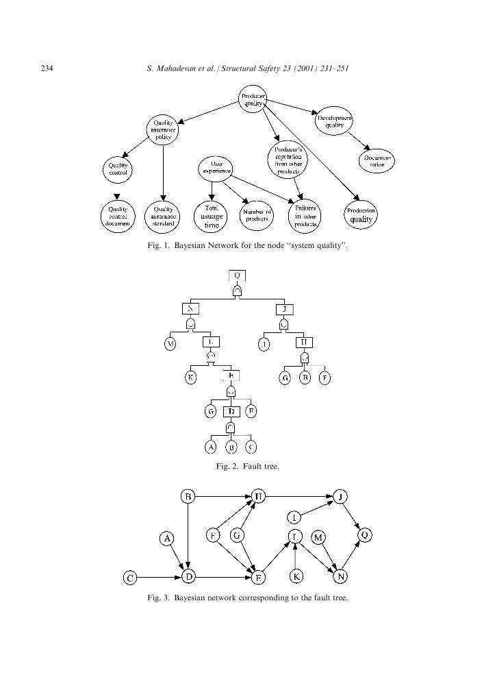
Fig. 1. Bayesian Network for the node ‘‘system quality’’.

Fig. 2. Fault tree.

Fig. 3. Bayesian network corresponding to the fault tree.


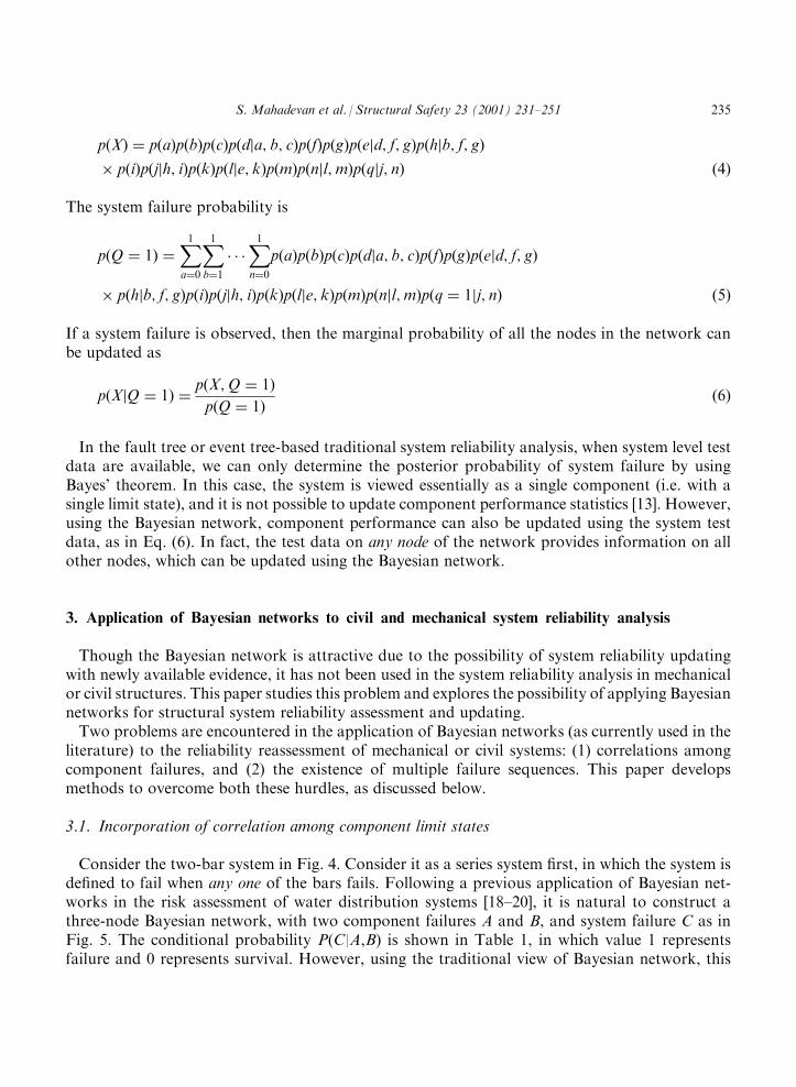
p Xð Þ ¼ p að Þp bð Þp cð Þp dja; b; cð Þp fð Þp gð Þp ejd; f; gð Þp hjb; f; gð Þ

� p ið Þp jjh; ið Þp kð Þp lje; kð Þp mð Þp njl;mð Þp qjj; nð Þ ð4Þ

The system failure probability is

p Q ¼ 1ð Þ ¼X1a¼0

X1b¼1

� � �X1n¼0

p að Þp bð Þp cð Þp dja; b; cð Þp fð Þp gð Þp ejd; f; gð Þ

� p hjb; f; gð Þp ið Þp jjh; ið Þp kð Þp lje; kð Þp mð Þp njl;mð Þp q ¼ 1jj; nð Þ ð5Þ

If a system failure is observed, then the marginal probability of all the nodes in the network canbe updated as

p XjQ ¼ 1ð Þ ¼p X;Q ¼ 1ð Þ

p Q ¼ 1ð Þð6Þ

In the fault tree or event tree-based traditional system reliability analysis, when system level testdata are available, we can only determine the posterior probability of system failure by usingBayes’ theorem. In this case, the system is viewed essentially as a single component (i.e. with asingle limit state), and it is not possible to update component performance statistics [13]. However,using the Bayesian network, component performance can also be updated using the system testdata, as in Eq. (6). In fact, the test data on any node of the network provides information on allother nodes, which can be updated using the Bayesian network.

3. Application of Bayesian networks to civil and mechanical system reliability analysis

Though the Bayesian network is attractive due to the possibility of system reliability updatingwith newly available evidence, it has not been used in the system reliability analysis in mechanicalor civil structures. This paper studies this problem and explores the possibility of applying Bayesiannetworks for structural system reliability assessment and updating.Two problems are encountered in the application of Bayesian networks (as currently used in the

literature) to the reliability reassessment of mechanical or civil systems: (1) correlations amongcomponent failures, and (2) the existence of multiple failure sequences. This paper developsmethods to overcome both these hurdles, as discussed below.

3.1. Incorporation of correlation among component limit states

Consider the two-bar system in Fig. 4. Consider it as a series system first, in which the system isdefined to fail when any one of the bars fails. Following a previous application of Bayesian net-works in the risk assessment of water distribution systems [18–20], it is natural to construct athree-node Bayesian network, with two component failures A and B, and system failure C as inFig. 5. The conditional probability P(C|A,B) is shown in Table 1, in which value 1 representsfailure and 0 represents survival. However, using the traditional view of Bayesian network, this


gives the impression that A and B are independent nodes and that there is no link between them.However, in this case, there is dependence between the failures of bar A and bar B. One kind ofdependence is the statistical correlation between the states of A and B due to the common randomvariables in their limit states. That means A and B are not independent even if they fail at the sametime, which is denoted as: P(AB)6¼P(A)P(B). However, the construction of Bayesian network inFig. 5 and the use of Eq. (1) lead to the result P(AB)=P(A)P(B), since according to the definitionof Bayesian network, A and B in Fig. 5 are root nodes, implying they are independent.To further illustrate this problem, using the algorithm of Eqs. (1) and (2), the series system

failure probability obtained from the Bayesian network in Fig. 5 and Table 1 is:

P C ¼ 1ð Þ ¼ 1:0� P A ¼ 1ð ÞPðB ¼ 1Þ þ 1:0� P A ¼ 1ð ÞPðB ¼ 0Þ þ 1:0� P A ¼ 0ð ÞPðB ¼ 1Þ

¼ PðA ¼ 1Þ þ PðB ¼ 1Þ 1� PðA ¼ 1Þ½

¼ PðA ¼ 1Þ þ PðB ¼ 1Þ � PðA ¼ 1ÞPðB ¼ 1Þ ð7Þ

We may simply write the result in Eq. (7) as PðAÞ þ PðBÞ � PðAÞPðBÞ. Since it is known that forthis series system, the failure probability is actually PðAÞ þ PðBÞ � PðA;BÞ, Eq. (7) is only correctwhen A and B are independent, which is not the case for this example. Therefore, the construc-tion in Fig. 5 needs to be modified to incorporate the dependence due to correlated limit states.To solve this problem, a new Bayesian network is constructed with all the input random vari-

ables as additional, but root nodes. For example, consider RA, the strength of A, RB, the strength of

Fig. 4. Two bar system.

Fig. 5. Bayesian network for the 2-bar system.

Table 1P(C=1jA, B) given the states of components A and B in a series system

A=1 A=0

B=1 1.0 1.0

B=0 1.0 0.0


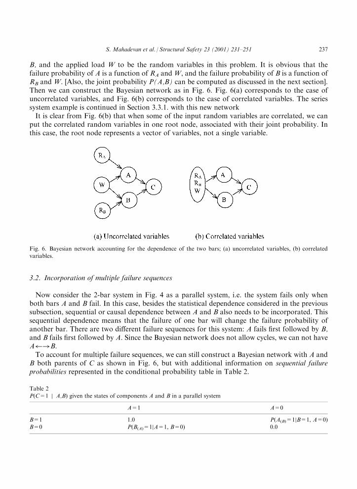
B, and the applied load W to be the random variables in this problem. It is obvious that thefailure probability of A is a function of RA andW, and the failure probability of B is a function ofRB andW. [Also, the joint probability P(A,B) can be computed as discussed in the next section].Then we can construct the Bayesian network as in Fig. 6. Fig. 6(a) corresponds to the case ofuncorrelated variables, and Fig. 6(b) corresponds to the case of correlated variables. The seriessystem example is continued in Section 3.3.1. with this new networkIt is clear from Fig. 6(b) that when some of the input random variables are correlated, we can

put the correlated random variables in one root node, associated with their joint probability. Inthis case, the root node represents a vector of variables, not a single variable.

3.2. Incorporation of multiple failure sequences

Now consider the 2-bar system in Fig. 4 as a parallel system, i.e. the system fails only whenboth bars A and B fail. In this case, besides the statistical dependence considered in the previoussubsection, sequential or causal dependence between A and B also needs to be incorporated. Thissequential dependence means that the failure of one bar will change the failure probability ofanother bar. There are two different failure sequences for this system: A fails first followed by B,and B fails first followed by A. Since the Bayesian network does not allow cycles, we can not haveA !B.To account for multiple failure sequences, we can still construct a Bayesian network with A and

B both parents of C as shown in Fig. 6, but with additional information on sequential failureprobabilities represented in the conditional probability table in Table 2.

Fig. 6. Bayesian network accounting for the dependence of the two bars; (a) uncorrelated variables, (b) correlated

variables.

Table 2P(C=1 j A,B) given the states of components A and B in a parallel system

A=1 A=0

B=1 1.0 P(A(B)=1jB=1, A=0)

B=0 P(B(A)=1jA=1, B=0) 0.0


In Table 2, A=1 and B=1 represent the failures of bars A and B starting from an intactstructure, A(B) represents the updated state of A after B’s failure, and B(A) represents the updatedstate of B after A’s failure. As an example, the relation P(C=1|A=1, B=0)=P(B(A)=1|A=1,B=0) means that the probability that C=1 will occur given A fails ‘‘first’’ is equal to B’s failureprobability given A fails ‘‘first’’, since C=1 is defined when both A and B fail. Through this con-struction of the conditional probability table for P(C=1|A, B), the problem of multiple failuresequences and the effect of the failure of one bar on another can be solved and incorporated in aBayesian network.Therefore, using the proposed approach, both types of dependence (statistical and sequential)

of the failure of the two bars are adequately incorporated in a Bayesian network. The statisticalcorrelation between the states of the components is incorporated by introducing the input ran-dom variables into the Bayesian network and taking them as root nodes. Sequential effects areincorporated through the definition of conditional system failure probability given a componentfailure sequence.

3.3. Implementation of system reliability analysis using the Bayesian network

3.3.1. Series systemBased on Eqs. (1) and (2), the probability of system failure in Fig. 6 for the series system can be

obtained as:

P C ¼ 1ð Þ ¼X1A¼0

X1B¼0

ðRA

ðRB

ðw

P C ¼ 1jA;Bð ÞP AjrA;wð ÞP BjrB;wð Þf rAð Þf rBð Þf wð ÞdrAdrBdw

¼

ðRA

ðRB

ðw

P A ¼ 0jrA;wð ÞP B ¼ 1jrB;wð Þf rAð Þf rBð Þf wð ÞdrAdrBdw

þ

ðRA

ðRB

ðw


þ

ðRA

ðRB

ðw

P A ¼ 1jrA;wð ÞP B ¼ 1jrB;wð Þf rAð Þf rBð Þf wð ÞdrAdrBdw ð8Þ

where f rAð Þ; f rBð Þandf wð Þ are the PDFs of the input random variables.Note that in this example, the three input random variables are taken as independent variables

for illustrative purposes. If they are correlated, the products of the three PDFs in the integrationin Eq. (8) will be replaced with their joint PDF.To further illustrate this problem, assume that Fig. 4 is a brittle structure, and each bar takes

half of the loadW. Then we can obtain the following conditional probabilities needed in Eq. (8):

P A ¼ 1jrA4w

2

� �¼ 1;P A ¼ 0jrA5

w

2

� �¼ 1 ð9aÞ

and

P B ¼ 1jrB4w

2

� �¼ 1;P B ¼ 0jrB5

w

2

� �¼ 1 ð9bÞ


Therefore Eq. (8) is written as:

P C ¼ 1ð Þ ¼

ðRA�

w2;RB�

w2

f rAð Þf rBð Þf wð ÞdrAdrBdwþ

ðRA�

w2;RB�

w2

f rAð Þf rBð Þf wð ÞdrAdrBdw

þ

ðRA�

w2;RB�

w2

f rAð Þf rBð Þf wð ÞdrAdrBdw ð10Þ

It can be also seen that each of the three terms on the right hand side of Eq. (8) is actually thelimit state-based joint probability of two correlated events, i.e.

P C ¼ 1ð Þ ¼ P A ¼ 0;B ¼ 1ð Þ þ P A ¼ 1;B ¼ 0ð Þ þ P A ¼ 1;B ¼ 1ð Þ

¼ P RA5w

2\ RB4

w

2

� �þ P RA4

w

2\ RB5

w

2

� �þ P RA4

w

2\ RB5

w

2

� �ð11Þ

The three terms in Eq. (11) can be calculated separately using system reliability methods (secondorder bounds [24], multi-normal integration [25], or Monte Carlo simulation) without completenumerical integration.Rewriting Eq. (11) as:

P C ¼ 1ð Þ ¼ P A ¼ 1;B ¼ 0ð Þ þ P A ¼ 1;B ¼ 1ð Þ þ P A ¼ 0;B ¼ 1ð Þ

¼ PðA ¼ 1Þ þ PðB ¼ 1Þ � PðA ¼ 1;B ¼ 1Þ

¼ P RA4w

2

� �þ P RB4

w

2

� �� P RA4

w

2\ RB4

w

2

� �ð12Þ

This is in the same form as derived by the usual series system reliability analysis, which demon-strates the validity of the new construction in Fig. 6 of the Bayesian network for this series system.Each term on the right hand side can be calculated using the reliability methods mentioned above.

3.3.2. Parallel systemConsider again the brittle structure in Fig. 4, where each bar carries half of the loadW. In this

case, if one bar fails, it is removed and subsequently the other bar will carry the entire load, andthe system failure is defined to occur when both bars fail. The limit state-based reliability methodin the previous subsection may also be used here for the computational implementation. Inaddition to the limit states for A= 1 and B=1 for the intact structure, the updated failure eventsof A(B) (A’s failure after B’s failure), and B(A) (B’s failure after A’s failure) also need to be definedto account for multiple failure sequences:

AðBÞ ¼ 1 ) RA4w

BðAÞ ¼ 1 ) RB4w ð13Þ

Therefore, combining the Bayesian network in Fig. 6, the conditional probability table inTable 2, and the limit state for each component, we obtain


PðC ¼ 1Þ ¼ P C ¼ 1jA ¼ 1;B ¼ 1ð Þ�P A ¼ 1;B ¼ 1ð Þ þ P C ¼ 1jA ¼ 0;B ¼ 1ð Þ�P A ¼ 0;B ¼ 1ð Þ

þ P C ¼ 1jA ¼ 1;B ¼ 0ð Þ � P A ¼ 1;B ¼ 0ð Þ þ P C ¼ 1jA ¼ 0;B ¼ 0ð Þ � P A ¼ 0;B ¼ 0ð Þ

¼ P RA �w

2\ RB4

w

2

� �þ P RA4wjRA5

w

2\ RB4

w

2

� �� P RA5

w

2\ RB4

w

2

� �

þ P RB � wjRA4w

2\ RB5

w

2

� �� P RA4

w

2\ RB5

w

2

� �

¼ P RA4w

2\ RB4

w

2

� �þ P RA4w \ RA5

w

2\ RB4

w

2

� �

þ P RB4w \ RA4w

2\ RB5

w

2

� �ð14Þ

To compare this result with the traditional reliability approach, consider the event tree method tocalculate the failure probability. The two failure sequences are represented by the followingintersections:

A ! B : RA4w

2\ RB4w B ! A : RB4

w

2\ RA4w

The system failure probability is the union of the two failure sequences:

Pf ¼ P RA4w

2\ RB4w

� �[ RB4

w

2\ RA4w

� �h i

¼ P RA4w

2\ RB4

w

2[w

24RB \ RB4w

� �� [

h

RB4w

2\ RA4

w

2[w

24RA \ RA4w

� �� i

¼ P RA4w

2\ RB4

w

2

� �[ RA4

w

2\w

24RB \ RB4w

� �[

h

RB4w

2\w

24RA \ RA4w

� �i

ð15Þ

Since the three events of the union in the final step in Eq. (15) are mutually exclusive, we have

Pf ¼ P RA4w

2\ RB4

w

2

� �þ P RA4

w

2\w

24RB \ RB4w

� �

þ P RB4w

2\w

24RA \ RA4w

� � ð16Þ

It can be seen that the system failure probability obtained by the Bayesian network in Eq. (14)and that calculated using the traditional system reliability method provide the exactly same resultfor this problem.Thus the proposed modifications to the traditional Bayesian network make it consistent for

application to structural system reliability analysis. However, the advantage of this approach isnot significant in system reliability prediction (forward propagation). Traditional fault-tree andevent-tree methods can already predict system reliability. (In fact, the Bayesian network needsmore computational effort to establish the conditional probability table, as discussed later inSection 4). The real advantage of the Bayesian network approach is in reliability reassessment(backward propagation), when new data becomes available. This is investigated in the next section.


3.4. Reliability updating using the Bayesian network

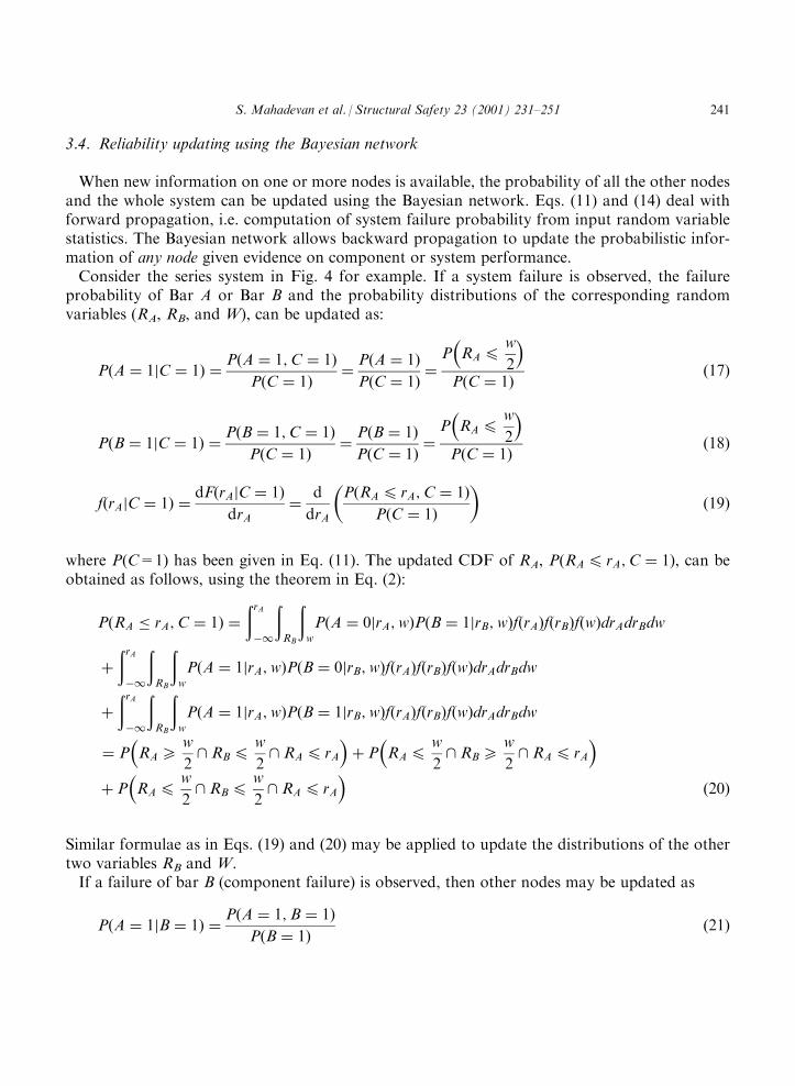
When new information on one or more nodes is available, the probability of all the other nodesand the whole system can be updated using the Bayesian network. Eqs. (11) and (14) deal withforward propagation, i.e. computation of system failure probability from input random variablestatistics. The Bayesian network allows backward propagation to update the probabilistic infor-mation of any node given evidence on component or system performance.Consider the series system in Fig. 4 for example. If a system failure is observed, the failure

probability of Bar A or Bar B and the probability distributions of the corresponding randomvariables (RA, RB, and W), can be updated as:

P A ¼ 1jC ¼ 1ð Þ ¼P A ¼ 1;C ¼ 1ð Þ

P C ¼ 1ð Þ¼P A ¼ 1ð Þ

P C ¼ 1ð Þ¼

P RA4w

2

� �P C ¼ 1ð Þ

ð17Þ

P B ¼ 1jC ¼ 1ð Þ ¼P B ¼ 1;C ¼ 1ð Þ

P C ¼ 1ð Þ¼P B ¼ 1ð Þ

P C ¼ 1ð Þ¼

P RA4w

2

� �P C ¼ 1ð Þ

ð18Þ

f rAjC ¼ 1ð Þ ¼dF rAjC ¼ 1ð Þ

drA¼

d

drA

P RA4 rA;C ¼ 1ð Þ

P C ¼ 1ð Þ

ð19Þ

where P(C=1) has been given in Eq. (11). The updated CDF of RA, P RA4 rA;C ¼ 1ð Þ, can beobtained as follows, using the theorem in Eq. (2):

P RA � rA;C ¼ 1ð Þ ¼

ðrA�1

ðRB

ðw


þ

ðrA�1

ðRB

ðw


þ

ðrA�1

ðRB

ðw


¼ P RA5w

2\ RB4

w

2\ RA4 rA

� �þ P RA4

w

2\ RB5

w

2\ RA4 rA

� �

þ P RA4w

2\ RB4

w

2\ RA4 rA

� �ð20Þ

Similar formulae as in Eqs. (19) and (20) may be applied to update the distributions of the othertwo variables RB and W.If a failure of bar B (component failure) is observed, then other nodes may be updated as

P A ¼ 1jB ¼ 1ð Þ ¼P A ¼ 1;B ¼ 1ð Þ

P B ¼ 1ð Þð21Þ


f rBjB ¼ 1ð Þ ¼dF rBjB ¼ 1ð Þ

drB¼

d

drB

P RB4 rB;B ¼ 1ð Þ

P B ¼ 1ð Þ

ð22Þ

Similar formulae may be applied to update the distributions of RA and W.Information on component failure can also be used to update the system failure probability

through the Bayesian network. In the case of the series system example, this is very simple:

P C ¼ 1jB ¼ 1ð Þ ¼P C ¼ 1;B ¼ 1ð Þ

P B ¼ 1ð Þ¼PðB ¼ 1Þ

PðB ¼ 1Þ¼ 1 ð23Þ

For the parallel system example,

P C ¼ 1jB ¼ 1ð Þ ¼P C ¼ 1;B ¼ 1ð Þ

P B ¼ 1ð Þ¼P C ¼ 1jA ¼ 0;B ¼ 1ð Þ � P A ¼ 0;B ¼ 1ð Þ

P B ¼ 1ð Þ

þP C ¼ 1jA ¼ 1;B ¼ 1ð ÞP A ¼ 1;B ¼ 1ð Þ

P B ¼ 1ð Þ

¼

P RA4w \ RA5w

2\ RB4

w

2

� �þ P RA4

w

2\ RB4

w

2

� �

P RB4w

2

� � ð24Þ

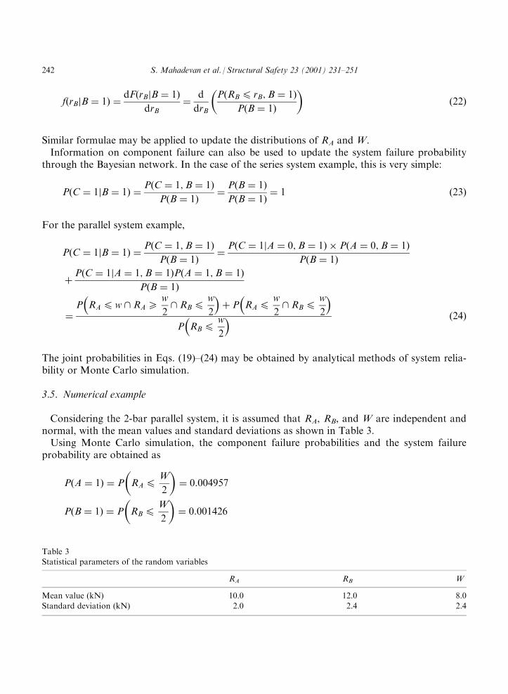
The joint probabilities in Eqs. (19)–(24) may be obtained by analytical methods of system relia-bility or Monte Carlo simulation.

3.5. Numerical example

Considering the 2-bar parallel system, it is assumed that RA, RB, and W are independent andnormal, with the mean values and standard deviations as shown in Table 3.Using Monte Carlo simulation, the component failure probabilities and the system failure

probability are obtained as

P A ¼ 1ð Þ ¼ P RA4W

2

¼ 0:004957

P B ¼ 1ð Þ ¼ P RB4W

2

¼ 0:001426

Table 3Statistical parameters of the random variables

RA RB W

Mean value (kN) 10.0 12.0 8.0

Standard deviation (kN) 2.0 2.4 2.4


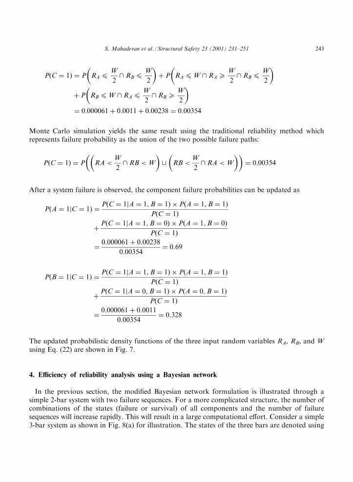
P C ¼ 1ð Þ ¼ P RA4W

2\ RB4

W

2

þ P RA4W \ RA5

W

2\ RB4

W

2

þ P RB4W \ RA4W

2\ RB5

W

2

¼ 0:000061þ 0:0011þ 0:00238 ¼ 0:00354

Monte Carlo simulation yields the same result using the traditional reliability method whichrepresents failure probability as the union of the two possible failure paths:

P C ¼ 1ð Þ ¼ P RA <W

2\ RB <W

[ RB <

W

2\ RA <W

¼ 0:00354

After a system failure is observed, the component failure probabilities can be updated as

P A ¼ 1jC ¼ 1ð Þ ¼P C ¼ 1jA ¼ 1;B ¼ 1ð Þ � P A ¼ 1;B ¼ 1ð Þ

P C ¼ 1ð Þ

þP C ¼ 1jA ¼ 1;B ¼ 0ð Þ � P A ¼ 1;B ¼ 0ð Þ

P C ¼ 1ð Þ

¼0:000061þ 0:00238

0:00354¼ 0:69

P B ¼ 1jC ¼ 1ð Þ ¼P C ¼ 1jA ¼ 1;B ¼ 1ð Þ � P A ¼ 1;B ¼ 1ð Þ

P C ¼ 1ð Þ

þP C ¼ 1jA ¼ 0;B ¼ 1ð Þ � P A ¼ 0;B ¼ 1ð Þ

P C ¼ 1ð Þ

¼0:000061þ 0:0011

0:00354¼ 0:328

The updated probabilistic density functions of the three input random variables RA, RB, and Wusing Eq. (22) are shown in Fig. 7.

4. Efficiency of reliability analysis using a Bayesian network

In the previous section, the modified Bayesian network formulation is illustrated through asimple 2-bar system with two failure sequences. For a more complicated structure, the number ofcombinations of the states (failure or survival) of all components and the number of failuresequences will increase rapidly. This will result in a large computational effort. Consider a simple3-bar system as shown in Fig. 8(a) for illustration. The states of the three bars are denoted using


A, B, C, and system failure is defined to occur when all the three bars fail, denoted by D=1. ABayesian network similar to Fig. 6 may be constructed. However, in this case, the conditionalprobability table P(D=1|A,B,C) will have 23 elements. We can easily have

Fig. 7. (a) Probability density function ofRA, (b) probability density function ofRB, (c) Probability density function ofW.


P D ¼ 1jA ¼ 1;B ¼ 1;C ¼ 1ð Þ ¼ 1

P D ¼ 1jA ¼ 0;B ¼ 0;C ¼ 0ð Þ ¼ 0

P D ¼ 1jA ¼ 1;B ¼ 1;C ¼ 0ð Þ ¼ P CðABÞ ¼ 1jA ¼ 1;B ¼ 1;C ¼ 0� �

P D ¼ 1jA ¼ 1;B ¼ 0;C ¼ 1ð Þ ¼ P BðACÞ ¼ 1jA ¼ 1;B ¼ 0;C ¼ 1� �

P D ¼ 1jA ¼ 0;B ¼ 1;C ¼ 1ð Þ ¼ P AðBCÞ ¼ 1jA ¼ 0;B ¼ 1;C ¼ 1� �

where C(AB)=1, B(AC)=1, A(BC)=1 are the failure events of the third bar after the other two barshave already failed. Their probabilities can be obtained through the updated limit states after thefailure of the other two bars. Then we look at the other three conditional probabilities:P(D=1|A=0,B=0,C=1), P(D=1|A=0,B=1,C=0), and P(D=1|A=1,B=0,C=0). Each oneof them is the failure probability of a two-bar system after the first failing bar has been removed,as shown in Fig. 9(a)–(c). To obtain any of these three terms, a sub-system failure probabilityanalysis has to be performed in which two failure sequences are involved, corresponding to thethree boxes in Fig. 8(b) of event tree of the system respectively.In the traditional event tree method, the system failure probability is calculated through the

union of all the failure sequences. In the Bayesian network analysis, it is seen that partial eventtree analysis is also needed for the conditional probability calculation. Therefore, the Bayesiannetwork approach has more computational effort than the event tree approach. However, thisextra effort provides a return by enabling backward propagation, that is, reliability re-assessment,when information about the system or any of the nodes becomes available.With the increase in the number of components, the conditional probability table will enlarge

geometrically and many of the terms will involve numerous sub-system failure analyses, whichmakes the computational implementation quite cumbersome. This restricts the application of acomplete Bayesian network to the system reliability analysis of practical structures.This problem exists even in traditional reliability analysis methods, since numerous potential

failure sequences exist in a large-scale structure. In reality, some have high probabilities ofoccurrence and others may have relatively low probabilities of occurrence. In such a case, the

Fig. 8. (a) 3-Bar truss system, (b) event tree of the 3-bar system.


reliability of the structural system is evaluated by selecting the probabilistically dominant failurepaths. Several methods, such as the branch and bound [5] or truncated enumeration [6] may beused for this selection. A failure sequence with a low failure probability is truncated before pro-ceeding to system failure, to avoid further enumeration. In this way, the insignificant failuresequences are discarded and the calculation of system failure probability is simplified.This paper uses the branch and bound concept for the construction of the conditional probability

table in the Bayesian network. The effects of the events with relatively very small probabilities areignored with their probabilities set to be zero. This approach is illustrated through a frame struc-ture shown in Fig. 10. Structural failure is defined as the formation of a collapse mechanism forwhich the bending moment is dominant. It is assumed that the loads P1 and P2 are uncorrelatednormal-distributed random variables and so are the bending moment capacities of the three framemembers. For illustrative purposes, all the numerical data are taken the same as in [5] and areshown in Table 4.The Bayesian network corresponding to the frame is constructed as in Fig. 11, in which S

denotes the state of the system. There are two states for the components and the system: 1representing failure and 0 representing survival. The failure domains Fi of the nodes 1, 2, 3, 4, 6, 7and 8 are obtained as

Fig. 9. Sub-system after the first bar’s failure.

Fig. 10. Geometry of frame and the locations of potential yield hinges.


F1 ¼ 1 :M1 ¼ R1 � 1:5038P1 þ 0:467P24 0

F2 ¼ 1 :M2 ¼ R2 þ 1:0009P1 � 0:9369P24 0

F3 ¼ 1 :M3 ¼ R3 þ 1:0009P1 � 0:9369P24 0

F4 ¼ 1 :M4 ¼ R4 � 0:0013P1 � 1:5631P24 0

F6 ¼ 1 :M6 ¼ R6 � 0:9982P1 � 0:9369P24 0

F7 ¼ 1 :M7 ¼ R7 � 0:9982P1 � 0:9369P24 0

F8 ¼ 1 :M8 ¼ R8 � 1:4971P1 � 0:467P24 0

The conditional probability table P(S=1|F1, F2,. . ..F8) will have 27=128 elements which needto be obtained through system reliability analysis separately. To make the computational imple-mentation feasible, the branch and bound method is used to select the significant failure sequen-ces and discard unimportant failure sequences and combinations of states of (F1. . .F8). Fivecomplete failure paths are selected, as shown in Fig. 12.From this, it is seen that the failure sequences originating from the failure of 1, 2, 3, and 6, are

all discarded due to their relatively low probability of occurrence. This means that the prob-abilities P(F1=1), P(F2=1), P(F3=1), and P(F6=1) are all very low and are ignored. Since themarginal probability P(F1=1) is very low, the joint probability of F1=1 and any combination ofstates of the other six nodes which is represented using P(F1=1, F2, F3, F4, F6, F7, F8) in thispaper, is even lower and approximated as zero in the conditional probability table. Similarly,P(F1, F2=1,F3, F4, F6, F7, F8)=0, P(F1, F2, F3=1, F4, F6, F7, F8)=0, and P(F1, F2, F3, F4,F6=1, F7, F8)=0.

Table 4Data for the frame structure

Plastic hinge location Cross sectionarea (m2)

Moment ofinertia (m4)

Mean value ofstrength R (kNm)

COV ofstrength R (kNm)

1,2 4.00�10�3 3.58�10�5 75.0 0.053,4 4.00�10�3 4.77�10�5 101.0 0.055,6 4.00�10�3 4.77�10�5 101.0 0.057,8 4.00�10�3 3.58�10�5 75.0 0.05

Young’s modulus: 210 GpaMean value of yield stress ��y¼276 MPa

P1 ¼ 20 kN, P2 ¼ 40 kN, COVRi=.05/0.3, COVPi=.05/0.3


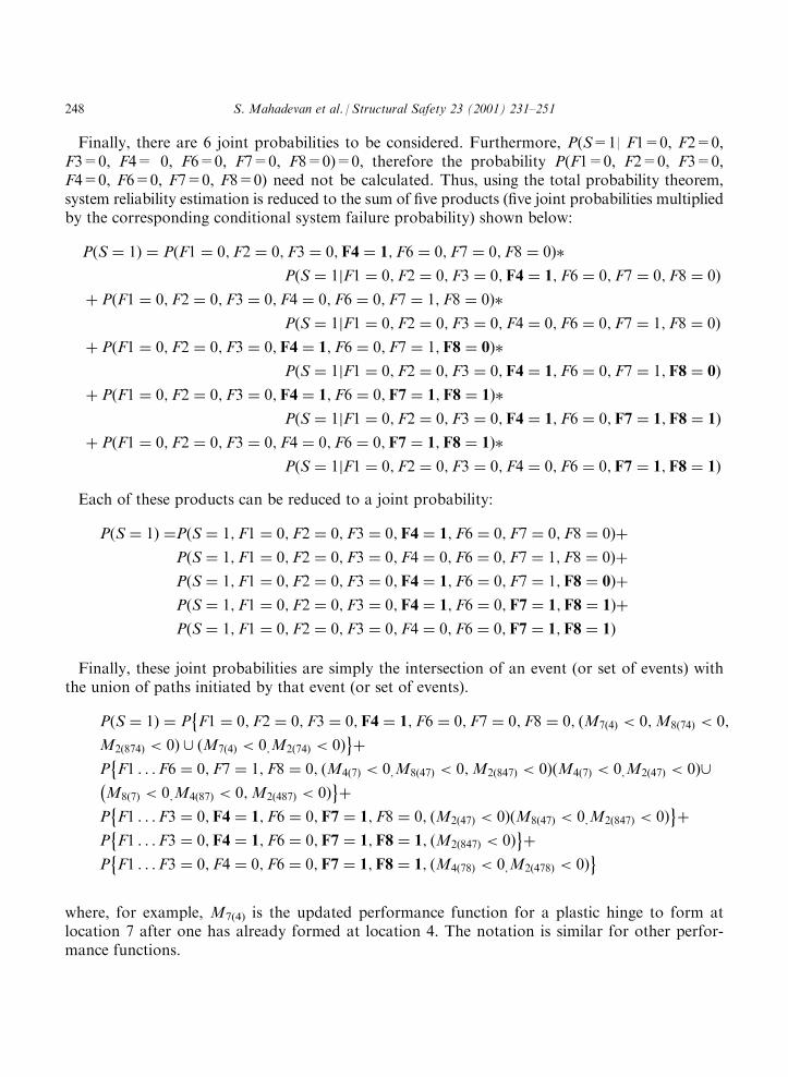
Finally, there are 6 joint probabilities to be considered. Furthermore, P(S=1| F1=0, F2=0,F3=0, F4= 0, F6=0, F7=0, F8=0)=0, therefore the probability P(F1=0, F2=0, F3=0,F4=0, F6=0, F7=0, F8=0) need not be calculated. Thus, using the total probability theorem,system reliability estimation is reduced to the sum of five products (five joint probabilities multipliedby the corresponding conditional system failure probability) shown below:

PðS ¼ 1Þ ¼ PðF1 ¼ 0;F2 ¼ 0;F3 ¼ 0;F4 ¼ 1;F6 ¼ 0;F7 ¼ 0;F8 ¼ 0Þ�

PðS ¼ 1jF1 ¼ 0;F2 ¼ 0;F3 ¼ 0;F4 ¼ 1;F6 ¼ 0;F7 ¼ 0;F8 ¼ 0Þ

þ PðF1 ¼ 0;F2 ¼ 0;F3 ¼ 0;F4 ¼ 0;F6 ¼ 0;F7 ¼ 1;F8 ¼ 0Þ�

PðS ¼ 1jF1 ¼ 0;F2 ¼ 0;F3 ¼ 0;F4 ¼ 0;F6 ¼ 0;F7 ¼ 1;F8 ¼ 0Þ

þ PðF1 ¼ 0;F2 ¼ 0;F3 ¼ 0;F4 ¼ 1;F6 ¼ 0;F7 ¼ 1;F8 ¼ 0Þ�

PðS ¼ 1jF1 ¼ 0;F2 ¼ 0;F3 ¼ 0;F4 ¼ 1;F6 ¼ 0;F7 ¼ 1;F8 ¼ 0Þ

þ PðF1 ¼ 0;F2 ¼ 0;F3 ¼ 0;F4 ¼ 1;F6 ¼ 0;F7 ¼ 1;F8 ¼ 1Þ�

PðS ¼ 1jF1 ¼ 0;F2 ¼ 0;F3 ¼ 0;F4 ¼ 1;F6 ¼ 0;F7 ¼ 1;F8 ¼ 1Þ

þ PðF1 ¼ 0;F2 ¼ 0;F3 ¼ 0;F4 ¼ 0;F6 ¼ 0;F7 ¼ 1;F8 ¼ 1Þ�

PðS ¼ 1jF1 ¼ 0;F2 ¼ 0;F3 ¼ 0;F4 ¼ 0;F6 ¼ 0;F7 ¼ 1;F8 ¼ 1Þ

Each of these products can be reduced to a joint probability:

PðS ¼ 1Þ ¼PðS ¼ 1;F1 ¼ 0;F2 ¼ 0;F3 ¼ 0;F4 ¼ 1;F6 ¼ 0;F7 ¼ 0;F8 ¼ 0Þþ

PðS ¼ 1;F1 ¼ 0;F2 ¼ 0;F3 ¼ 0;F4 ¼ 0;F6 ¼ 0;F7 ¼ 1;F8 ¼ 0Þþ

PðS ¼ 1;F1 ¼ 0;F2 ¼ 0;F3 ¼ 0;F4 ¼ 1;F6 ¼ 0;F7 ¼ 1;F8 ¼ 0Þþ

PðS ¼ 1;F1 ¼ 0;F2 ¼ 0;F3 ¼ 0;F4 ¼ 1;F6 ¼ 0;F7 ¼ 1;F8 ¼ 1Þþ

PðS ¼ 1;F1 ¼ 0;F2 ¼ 0;F3 ¼ 0;F4 ¼ 0;F6 ¼ 0;F7 ¼ 1;F8 ¼ 1Þ

Finally, these joint probabilities are simply the intersection of an event (or set of events) withthe union of paths initiated by that event (or set of events).

PðS ¼ 1Þ ¼ P F1 ¼ 0;F2 ¼ 0;F3 ¼ 0;F4 ¼ 1;F6 ¼ 0;F7 ¼ 0;F8 ¼ 0; ðM7ð4Þ < 0;M8ð74Þ < 0;

M2ð874Þ < 0Þ [ ðM7ð4Þ < 0;M2ð74Þ < 0Þ�þ

P F1 . . .F6 ¼ 0;F7 ¼ 1;F8 ¼ 0; ðM4ð7Þ < 0;M8ð47Þ < 0;M2ð847Þ < 0ÞðM4ð7Þ < 0;M2ð47Þ < 0Þ[ M8ð7Þ < 0;M4ð87Þ < 0;M2ð487Þ < 0Þ� �

þ

P F1 . . .F3 ¼ 0;F4 ¼ 1;F6 ¼ 0;F7 ¼ 1;F8 ¼ 0; ðM2ð47Þ < 0ÞðM8ð47Þ < 0;M2ð847Þ < 0Þ �

þ

P F1 . . .F3 ¼ 0;F4 ¼ 1;F6 ¼ 0;F7 ¼ 1;F8 ¼ 1; ðM2ð847Þ < 0Þ �

þ

P F1 . . .F3 ¼ 0;F4 ¼ 0;F6 ¼ 0;F7 ¼ 1;F8 ¼ 1; ðM4ð78Þ < 0;M2ð478Þ < 0Þ �

where, for example, M7(4) is the updated performance function for a plastic hinge to form atlocation 7 after one has already formed at location 4. The notation is similar for other perfor-mance functions.


Using Monte Carlo simulation, system failure is computed as

PðS ¼ 1Þ ¼ :0003þ 0þ :0054þ :0009þ 0 ¼ 0:0066

The same system failure can be calculated with the traditional method of taking the union ofthe five significant failure paths:

PðS ¼ 1Þ ¼ P ðM7 < 0;M4ð7Þ < 0;M8ð47Þ < 0;M2ð847Þ < 0ÞðM7 < 0;M4ð7Þ < 0;M2ð47Þ < 0Þ[

M7 < 0;M8ð7Þ < 0;M4ð87Þ < 0;M2ð487Þ < 0Þ [ ðM4 < 0;M7ð4Þ < 0;M8ð74Þ < 0;M2ð874Þ < 0Þ�[ðM4 < 0;M7ð4Þ < 0;M2ð74Þ < 0Þ

�¼ 0:0066

During forward propagation to calculate system failure, the proposed method does not provideany result different from the traditional system reliability method. In fact, it requires extra calcu-lations to compute the probabilities of several subsystems (for example, the three subsystems a, b,and c in Fig. 12). The advantage of this extra computation is that it facilitates backward propa-gation for updating the conditional probabilities after system performance information isobtained. In the forward propagation, the estimates of overall system failure probability, branchprobabilities, and correlation effects will be same as that obtained using the traditional systemreliability method.As can be seen, the use of the branch and bound approach makes the proposed Bayesian net-

work method feasible for reliability reassessment and updating. The accuracy of the approxima-tion depends on the criterion used to discard a failure sequence in the branch-and-boundapproach.Given new information on system performance (failure or survival), the probability of plastic

hinge formation at a specific location can be updated. For example, if system collapse is observed,we obtain

P F4 ¼ 1jS ¼ 1ð Þ ¼PðF4 ¼ 1;S ¼ 1Þ

PðS ¼ 1Þ¼0:66

0:66¼ 1

P F7 ¼ 1jS ¼ 1ð Þ ¼PðF7 ¼ 1;S ¼ 1Þ

PðS ¼ 1Þ¼0:0064

0:0066¼ 0:970

Note that in the above forward and backward propagation, all the terms corresponding to thejoint probabilities, P(F1=1, F2, F3, F4, F6, F7, F8), P(F1, F2=1, F3, F4, F6, F7, F8), P(F1, F2,F3=1, F4, F6, F7, F8), and P(F1, F2, F3, F4, F6=1, F7, F8), are omitted due to their relativelylow values. This approximation will result in the updated failure probabilities P(F1=1|S=1),P(F2=1|S=1), P(F3=1|S=1) and P(F6=1|S=1) all equal to zero. Since 4 and 7 are the twoweakest locations where plastic hinge most probably forms, their updated failure probabilities areof most concern, compared to the other locations. However, in the case that the failure prob-abilities—original evaluation and/or posterior updating—at other locations also need to be con-sidered, the branch-and-bound method may be modified by previewing all the potential plastichinges after the first branching operation, and bounding only in the subsequent steps.


5. Conclusion

A new methodology has been developed in this paper for the application of the Bayesian net-work concept to structural system reliability reassessment. Multiple failure sequences and corre-lations between component failures are considered and incorporated in the Bayesian networkconstruction. The proposed approach to include these two additional features is validated bycomparing it with the results of traditional reliability analysis. Both forward and backward pro-pagation formulae are developed. In order to extend the method to the application of morecomplicated structures, the Bayesian network is combined with the branch-and-bound method toconsider only the significant failure sequences. A frame structure with multiple potential locationsof plastic hinges and multiple failure sequences is analyzed to illustrate the proposed approach.The numerical result shows that the combination of Bayesian network and branch and boundapproach considerably improves the efficiency of the method and makes it applicable to thereliability reassessment of large structures, when new data on structural performance becomesavailable.The proposed reliability reassessment approach applies the Bayesian network to both forward

and backward uncertainty propagation between component and system performance, and solvesthe problem of information transformation from system level to component level. Since most realstructures involve multiple components and multiple failure sequences, the proposed modifica-tions in the Bayesian network facilitate a comprehensive framework for system reliability reas-sessment.

Acknowledgements

The research reported in this paper was supported by funds from Sandia National Labora-tories, Albuquerque, NM (Contract No. BG-7732), under the Sandia/NSF Life Cycle Engineer-ing Program (Project Monitors: Dr. David Martinez, Dr. Steve Wojtkiewicz). The support isgratefully acknowledged. Sandia is a multi-program laboratory operated by Sandia Corporation,a Lockheed Martin Company, for the US Department of Energy under Contract DE-AC04-94AL85000.

References

[1] Madsen HO. Model updating in reliability theory. Proceeding of ICASP-5, 1987, Vancouver. pp. 564–77.[2] Zhao Z, Haldar A, Breen FL. Fatigue-reliability updating through inspection of steel bridges. Journal of Struc-

tural Engineering ASCE 1994;120(5):1624–41.

[3] Byers WG, Marley MJ, Mohammadi J, Nielsen RJ, Sarkani S. Fatigue reliability reassessment procedures: state-of-the art paper. Journal of Structural Engineering ASCE 1994;123(3):271–6.

[4] Zheng R, Ellingwood B. Role of non-destructive evaluation in time-dependent reliability analysis. Structural

Safety 1998;20(4):325–39.[5] Thoft-Christensen P, Murotsu Y. Application of structural reliability theory. New York: Springer, 1986.[6] Melchers RE, Tang LK. Failure modes in complex stochastic systems. In: Proceeding of the 4th international

conference on structural safety and reliability. ICOSSAR’85, Kobe, Japan, 1985. p. 97–106.[7] Moses F. System reliability developments in structural engineering. Structural Safety 1982;1:3–13.


[8] Fu G, Moses F. Importance sampling in structural system reliability. In: Proceedings of ASCE joint specialty

conference on probabilistic methods. Blacksburg, VA, 1988. p. 340-3.[9] Xiao Q, Mahadevan S. Fast failure mode identification for ductile structural system reliability. Structural Safety

1994;13:207–26.

[10] Cole PVZ. A Bayesian reliability assessment of complex systems for binomial sampling. IEEE Transactions onReliability 1975;24:114–7.

[11] Mastran DV, Singpurwalla ND. A Bayesian estimation of the reliability of coherent structures. Operations

Research 1978;26:663–72.[12] Thompson WE, Haynes RD. On the reliability, availability, and Bayes confidence intervals for multi-component

systems. Naval Research Logistic Quarterly 1980;27:354–8.[13] Martz HF, Waller PA. Bayesian reliability analysis. New York: John Wiley & Sons, 1982.

[14] Jensen FV. An introduction to Bayesian network. New York: Springer, 1996.[15] Dahll G. Combining disparate sources of information in the safety assessment of software-based systems. Nuclear

Engineering and Design 2000;195:307–19.

[16] Friis-Hansen A, Friis-Hansen P, Christensen CF. Reliability analysis of upheaval buckling-updating and costoptimization. In: Proceeding 8th ASCE specialty conference on probabilistic mechanics and structural reliability,Notre Dame, 2000.

[17] Treml CA, Dolin RM, Shah NB. Using Bayesian belief networks and an as-built/as-is assessment for quantifyingand reducing uncertainty in prediction of buckling characteristic of spherical shells. In: Proceeding 8th ASCEspecialty conference on probabilistic mechanics and structural reliability, Notre Dame, 2000.

[18] Castillo E, Solares C, Gomez P. Estimating extreme probabilities using tail simulated data. International Journalof Approximate Reasoning 1997;17:163–89.

[19] Castillo E, Gutierrez JM, Hadi AS. Goal-oriented symbolic propagation in Bayesian networks. In: Proceedings ofthe thirteenth national conference on artificial intelligence (AAAI’96), Portland, OR Menlo Park, CA, AAI Press-

MIT Press, 1996. p. 1263–8.[20] Castillo E, Sarabia JM, Solares C, Gomez P. Uncertainty analysis in fault trees and Bayesian networks using

FORM/SORM methods. Reliability Engineering and System Safety 1999;65(1):29–40.

[21] Henrion M. Some practical issue in constructing belief networks. In: Kanal, LN, Levitt, TS, Lemmer, JF, editors.Uncertainty in artificial intelligence 1. Amsterdam, Holland, 1989.

[22] Fung R, Chang K. Weighing and integrating evidence for stochastic simulation in Bayesian Networks. In: Hen-

rion M, Shachter RD, Kanal LN, Lemmer JF, editors. Uncertainty in artificial intelligence 2, Amsterdam, Hol-land, 1990.

[23] Bouckaert RR, Castillo E, Gutierrez JM. A modified simulation Scheme for inference in Bayesian networks.

International Journal of Approximate Reasoning 1996;14:55–80.[24] Xiao Q, Mahadevan S. Second-order upper bounds on probability of intersection of failure events. Journal of

Engineering Mechanics, ASCE 1998;120(3):670–5.[25] Gollwitzer S, Rackwitz R. An efficient numerical solution to the multinormal integral. Probabilistic Engineering

Mechanics 1988;3:98–101.


Documents

Bayesian networks for system reliability reassessment