Original Article

Proc IMechE Part M:J Engineering for the Maritime Environment227(2) 107–113� IMechE 2013Reprints and permissions:sagepub.co.uk/journalsPermissions.navDOI: 10.1177/1475090212454385pim.sagepub.com

Dynamics and robust control ofunderwater vehicles for depthtrajectory following

S-S You1, T-W Lim2, J-Y Kim3 and H-S Choi1

AbstractThis paper addresses the robust control synthesis of diving/climbing manoeuvres for underwater vehicle in the verticalplane. First, a new state–space representation for the vehicle dynamics is presented, and the corresponding problem for-mulation is clearly stated. Next, the two-controller set-up using a H‘-loop shaping design is employed to deal with thebottom following capability and robustness issues. Then the reduced order control system with a Hankel norm is evalu-ated in the frequency domain. In addition, the preview control approach is used to improve the overall tracking perfor-mance for undersea manoeuvres. The specific control tasks include the tracking of a set of depth profiles or oceanfloors. Simulation results show that control objectives are effectively accomplished in spite of model uncertainties.Finally, it is found that the proposed control methodology is suitable for the depth trajectory following applications overa wide range of operating conditions.

KeywordsUnderwater vehicles, vertical plane, loop-shaping design, robust controller

Date received: 7 February 2012; accepted: 6 June 2012

Introduction

Over the last two decades, autonomous underwatervehicles (AUVs) have been steadily growing as a majortopic for underwater research. The costs and the risksassociated with various undersea tasks can be reducedusing underwater vehicles. Typical applications includeoceanographic survey, ocean floor analysis, militaryoperations, and underwater construction. This has ledto an increase in the demand for various underwatercapabilities to perform high-precision tasks.

Since AUV dynamics are highly nonlinear andcoupled, the corresponding control synthesis is challen-ging for uncertain operation scenarios. In addition, itshould be noted that underwater vehicles use multiplecontrol surfaces to perform efficient manoeuvres. Thecontrol systems in use include various control algo-rithms, based on linear or nonlinear controlapproaches.1–3 Sliding mode control scheme usingswitching algorithm is proposed for dynamic position-ing of AUVs.4 However, it is well known that thismethod is susceptible to a high frequency chatteringeffect on the control signal. The neuro-fuzzy controllerhas proven to be a good option for underwater vehiclecontrol; however, normally it requires a long tuning

process for the system parameters.5 Due to its simplestructure, an adaptive control law with a proportional-derivative (PD) action has been proposed by Antonelliet al.6 In reality, the controller design resulting fromthis classical approach does not provide satisfactoryperformance or robustness with respect to uncertain-ties. The H‘ control approach was introduced for therobust stabilization of the uncertain plant.7 Basically,the robustness of the control system has been a primaryreason for the application of advanced control theory.It should be noted that the loop shaping design withthe H‘ approach provides a computationally efficientalgorithm and robustness without explicit knowledgeof the uncertainties.8,9 In a multi-objective control

1Division of Mechanical and Energy Systems Engineering, Korea Maritime

University, Busan, Republic of Korea2Division of Marine Engineering, Korea Maritime University, Busan,

Republic of Korea3Division of Marine Equipment Engineering, Korea Maritime University,

Busan, Republic of Korea

Corresponding author:

T-W Lim, Division of Marine Engineering, Korea Maritime University,

Dongsam-dong, Yeongdo-ku, Busan, 606-791, Republic of Korea.

Email: kyunlim@hhu.ac.kr

synthesis, a single controller often leads to poor stabi-lity and performance. In particular, the two-degree-of-freedom (2-DOF) controller9–11 offers high-performance for multivariable control systems. Fortypical underwater applications, various control taskshave to be performed in the vertical plane: bottom fol-lowing, depth changing and station keeping.4,12 Somecontrol approaches use vision-based algorithms, butthese are not a practical choices due to visibility issuesin the underwater environment.13 The path-followingcontrol of underwater vehicles is discussed, for exam-ple, in Aguiar and Hespanha14 and Lapierre andJouvencel,15 and bottom-following problems are dis-cussed in Paulino et al.16 Moreover, it is desirable toreduce the size of the robust controllers for real imple-mentation.17 Even though various kinds of control sys-tems for underwater vehicles have been reported andconstructed, the related design technologies are notfully matured, especially in implementing robust con-trol systems. This study is extensively concerned withrobust controller design for undersea vehicles using aloop shaping approach with singular values.

Kinematics and dynamics for verticalmanoeuvres

In this paper, a torpedo shaped vehicle manoeuvresalong a set of depth/altitude trajectories in the vertical

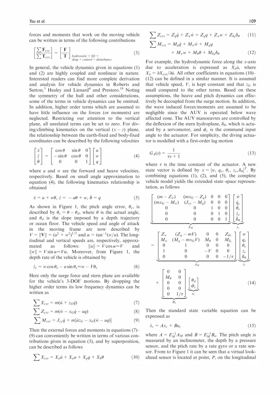
plane. The kinematic relationship and dynamic equa-tions of the vehicle can be developed using two coordi-nate systems; the earth-fixed (inertial) frame, fUg : =(O-X,Y,Z), and the body-fixed frame, fBg : =(o-x,y,z) as depicted in Figure 1. The origin, o, of the bodyframe, fBg, is fixed at the centre of buoyancy, CB.Then, the vector rG = ½xG, yG, zG�Trepresents the coor-dinates of the centre of gravity, CG, with respect to CB,drawn from o on the vehicle body. The CB is assumedas not coincident with the CG.

Using the Newton–Euler formulation, the rigid-body(translational and rotational) dynamics for a vehiclemoving in the inertial frame is described as follows

XFext =m _V+Ω3V+ _Ω3rG +Ω3(Ω3rG)

� �ð1ÞX

Text = J _Ω+Ω3(JΩ)+mrG3 _V+Ω3V� �

ð2Þ

whereP

Fext= ½Xext, Yext, Zext�TandP

Text = ½Kext,Mext, Next�T are the vectors of external forces andmoments decomposed in the moving frame, fBg,respectively; V= ½u, v,w�T is the linear velocity (surge,sway, heave) decomposed in fBg; J= diag(Jxx, Jyy, Jzz)is the moment of inertia matrix about principal axes(x,y,z) of the frame fBg, J= JT . 0; Ω= ½p, q, r�T isthe angular velocity (roll, pitch, and yaw rate) of theframe fBg relative to the inertial frame. The external

Figure 1. Coordinate frames and motion variables in the vertical plane.

108 Proc IMechE Part M: J Engineering for the Maritime Environment 227(2)

forces and moments that work on the moving vehiclecan be written in terms of the following contributionsP

FextPText

� �=

F

T

� �hydrostatic+ lift+drag+ control+ disturbance

ð3Þ

In general, the vehicle dynamics given in equations (1)and (2) are highly coupled and nonlinear in nature.Interested readers can find more complete derivationand analysis for vehicle dynamics in Roberts andSutton,3 Healey and Lienard4 and Prestero.18 Notingthe symmetry of the hull and other considerations,some of the terms in vehicle dynamics can be omitted.In addition, higher order terms which are assumed tohave little influence on the forces (or moments) areneglected. Restricting our attention to the verticalplane, all unrelated terms can be set to zero. For div-ing/climbing kinematics on the vertical (x� z) plane,the relationship between the earth-fixed and body-fixedcoordinates can be described by the following velocities

_x_z_u

2435=

cos u sin u 0� sin u cos u 0

0 0 1

24

35 u

wq

24

35 ð4Þ

where u and w are the forward and heave velocities,respectively. Based on small angle approximation toequation (4), the following kinematics relationship isobtained

_x= u+wu, _z= � uu+w, _u= q ð5Þ

As shown in Figure 1, the pitch angle error, ue, isdescribed by ue = u� ud, where u is the actual angle,and ud is the slope imposed by a depth trajectoryor ocean floor. The vehicle speed and angle of attackin the moving frame are now described byV= Vk k=(u2 +w2)1=2 and a=tan�1(w=u). The long-itudinal and vertical speeds are, respectively, approxi-mated as follows: uk k=V cosa’V andwk k=V sina’Va. Moreover, from Figure 1, thedepth rate of the vehicle is obtained by

_ze =w cos ue � u sin ue’w� Vue ð6Þ

Here only the surge force and stern plane are availablefor the vehicle’s 3-DOF motions. By dropping thehigher order terms its low frequency dynamics can bewritten asX

Xext =m( _u+ zG _q) ð7ÞXZext =m( _w� xG _q� uq) ð8ÞXMext = Jyy _q+m½ _uzG � xG( _w� uq)� ð9Þ

Then the external forces and moments in equations (7)–(9) can conveniently be written in terms of various con-tributions given in equation (3), and by superposition,can be described as followsX

Xext =X _u _u+Xuu+Xqq+Xuu ð10Þ

XZext =Z _q _q+Z _w _w+Zqq+Zww+Zdu

du ð11ÞXMext=M _q _q+M _w _w+Mqq

+Mww+Muu+Mdudu ð12Þ

For example, the hydrodynamic force along the x-axisdue to acceleration is expressed as X _u _u, whereX _u = ∂Xext=∂ _u. All other coefficients in equations (10)–(12) can be defined in a similar manner. It is assumedthat vehicle speed, V, is kept constant and that zG issmall compared to the other terms. Based on theseassumptions, the heave and pitch dynamics can effec-tively be decoupled from the surge motion. In addition,the wave induced forces/moments are assumed to benegligible since the AUV is operated below waveaffected zone. The AUV manoeuvres are controlled bythe deflexion of the stern hydroplane, du, which is actu-ated by a servomotor, and fc is the command inputangle to the actuator. For simplicity, the diving actua-tor is modelled with a first-order lag motion

GA(s)=1

ts+1ð13Þ

where t is the time constant of the actuator. A newstate vector is defined by x= ½w, qe, ue, ze, du�T. Bycombining equations (1), (2), and (5), the completevehicle model yields the extended state–space represen-tation, as follows

(m� Z _w) (mxG � Z _q) 0 0 0(mxG �M _w) (Jyy �M _q) 0 0 0

0 0 1 0 00 0 0 1 00 0 0 0 1

266664

377775

|fflfflfflfflfflfflfflfflfflfflfflfflfflfflfflfflfflfflfflfflfflfflfflfflfflfflfflfflfflfflfflfflfflfflfflfflfflffl{zfflfflfflfflfflfflfflfflfflfflfflfflfflfflfflfflfflfflfflfflfflfflfflfflfflfflfflfflfflfflfflfflfflfflfflfflfflffl}EM

_w_qe_ue

_ze_du

266664

377775

|fflffl{zfflffl}_xc

=

Zw (Zq �mV) 0 0 Zds

Mw (Mq �mxGV) Mu 0 Mds

0 1 0 0 01 0 �V 0 00 0 0 0 �1=t

266664

377775

|fflfflfflfflfflfflfflfflfflfflfflfflfflfflfflfflfflfflfflfflfflfflfflfflfflfflfflfflfflfflfflfflfflfflfflfflfflffl{zfflfflfflfflfflfflfflfflfflfflfflfflfflfflfflfflfflfflfflfflfflfflfflfflfflfflfflfflfflfflfflfflfflfflfflfflfflffl}AM

wqeue

zedu

266664

377775

|fflffl{zfflffl}xc

+

0 0Mu 00 00 00 1=t

266664

377775

|fflfflfflfflfflfflfflfflffl{zfflfflfflfflfflfflfflfflffl}Bu

ud

fc

� �|fflffl{zfflffl}

uc

ð14Þ

Then the standard state variable equation can beexpressed as

_xc =Axc+Buc ð15Þ

where A=E�1M AM and B=E�1M Bu. The pitch angle ismeasured by an inclinometer, the depth by a pressuresensor, and the pitch rate by a rate gyro or a rate sen-sor. From to Figure 1 it can be seen that a virtual look-ahead sensor is located at point, P, on the longitudinal

...............

You et al. 109

axis with a preview distance lp.9,16 Then its vertical dis-

placement from the reference trajectory is described by

hp = ze + lpue ð16Þ

where the vertical offset, ze, is defined as the perpendi-cular distance of the vehicle at CB from the referencetrajectory. The system output vector is given by the vec-tor of variables, yc = ½u, p, hp�T, which are directly mea-sured or effectively estimated by sensors. The outputequation is written as

yc(t)=Cxc(t)+Duc(t) ð17Þ

where the output matrices are given by

C=

0 0 1 0 00 1 0 0 00 0 lp 1 0

24

35, D=

1 00 00 0

24

35

For the state–space realisation using equations (15) and(17), the guidance and control systems for AUV can bedeveloped: vehicle guidance rules are based on kine-matic relationships whereas control systems aredesigned based on vehicle dynamics.

Robust control synthesis

The vehicle system is given in state–space form, and thetransfer function for the nominal model Gn(s) can bedefined by

Gn(s)=A BC B

� �=C(sI� A)�1B+D ð18Þ

where the nominal values for the vehicle parametersbeing considered are given in Table 1. For the loop-shaping design, the nominal system is augmented withpre- and post-compensators using weighting functionsW1(s) andW2(s), respectively. The shaped vehicle modelis then described by using a left co-prime factorisation8

Gs(s)=W2GnW1 =M�1s Ns ð19Þ

where the co-prime matrices (Ms,Ns) are stable andproper. Some features are worthy of comment in con-nection with the loop-shaping design. The compensa-tors are introduced to shape the nominal plant for thedesired open-loop gains (GsK). Typically, the loopgains are large at low frequencies to provide

disturbance rejection and reference tracking. In addi-tion, the loop gains are small at high frequencies toachieve noise attenuation, control energy reductionand robust stability. In multi-objective control synth-esis with a particularly under-actuated system, thedesign goals are not accomplished simultaneouslywith total success. As an alternative structure, illu-strated in Figure 2, the control system with two-controller set-up is partitioned as K= ½K1 K2�, whereK1 is the command compensator designed to reachthe required specifications in the time domain, and K2

is the feedback controller guaranteeing the systemstability.10,11 It is worth noting that Ld represents thedesired closed-loop transfer function between ra andyc. In addition, the parameter l is used to weigh therelative importance of robust stability as compared tomodel-matching and the gain matrix, Wc has beenadded for output variable selection.

With reference to the system set-up, the vehicle plantwith additive perturbation is given by

GD(s)= (Ms +DM)�1(Ns +DN) : Dk k‘ \ e= g�1� �

,

D= ½DN, � DM� ð20Þ

where all plant uncertainties, which are described byunmodelled dynamics or parametric perturbations, canbe given by a uncertainty matrix, D.

As depicted in Figure 2, some vector-valued signalsare described as follows: the control inputs, us, the mea-sured variables, ys, command signals, ra, the scaled ref-erence signals, rc, the control error signals, e and theperturbation inputs, wp.

The generalised AUV model is now derived by rear-ranging the control system. It is noted that the plantconsists of the physical plant to be controlled, togetherwith appended weights that shape the exogenous andinternal signals. Then, the generalised plant, ,P(s) is fur-ther written as

usyserays

266664

377775=

0 0 IM�1s 0 Gs

lWcM�1s �l2Ld lWcGs

0 lI 0M�1s 0 Gs

266664

377775

|fflfflfflfflfflfflfflfflfflfflfflfflfflfflfflfflfflfflfflfflfflfflfflfflfflfflfflffl{zfflfflfflfflfflfflfflfflfflfflfflfflfflfflfflfflfflfflfflfflfflfflfflfflfflfflfflffl}P(s)

wp

rcus

24

35,

wp =Dusys

� �and us =K

rays

� �ð21Þ

Using linear fractional transformation (LFT), theclosed-loop system, FL(P,K), is described by

usyse

24

35=

K2(I� GsK2)�1M�1s l(I� K2Gs)

�1K1

(I� GsK2)�1M�1s l(I� GsK2)

�1GsK1

lWc(I� GsK2)�1M�1s l2½Wc(I� GsK2)

�1GsK1 � Ld�

264

375

|fflfflfflfflfflfflfflfflfflfflfflfflfflfflfflfflfflfflfflfflfflfflfflfflfflfflfflfflfflfflfflfflfflfflfflfflfflfflfflfflfflfflfflfflfflfflfflfflfflfflfflfflfflfflffl{zfflfflfflfflfflfflfflfflfflfflfflfflfflfflfflfflfflfflfflfflfflfflfflfflfflfflfflfflfflfflfflfflfflfflfflfflfflfflfflfflfflfflfflfflfflfflfflfflfflfflfflfflfflfflffl}FL(P,K)

wp

rc

� �

ð22Þ

............

..........................................................

.................. .......................................... ....

....

....

.......

..................

Table 1. Underwater vehicle parameters.3,18

Parameters Nominal value Parameters Nominal value

m 30.48 (kg) M _w 21.93 (kg.m)V 1.54 (m/s) M _q 24.88 (kg.m2)Jyy 3.43 (kg m2/rad) Mw 3.07 (kg.m/s)Z _w 23:5531001(kg) Mq 26.87 (kg.m2/s)Z _q 21.93 (kg m/rad) Mu 25.77 (kg.m2/s2)Zw 26:6631001(kg/s) Mds 23.46 (kg.m2/s2)Zq 29.67 (kg m/s) Zds 25.06 (kg.m/s2)

Hull length: 1.5 (m), t: 0.15 (s), zG = 1:96310�02 (m), xG = yG = 0 (m).

110 Proc IMechE Part M: J Engineering for the Maritime Environment 227(2)

According to the generalised control framework, thesuboptimal H‘ control synthesis can be written as7

FL(P,K)k k‘ \ g, with go = infstabilizing K

FL(P,K)k k‘

ð23Þ

where g (5go) is a constant for a pre-specified perfor-mance level. Specifically, the purpose of the precompen-sator is to ensure that the output of the actual plant,La(s), tracks that of Ld(s) for model matching such that

La(s)� Ld(s)k k‘4g=l2 ð24Þ

where La(s)=Wc(I� GsK2)�1GsK1 is the transfer

function between ra and yc. For the steady-state gainmatching, the command signals, rc, can be scaled by aconstant matrix, Lcm, to make the transfer functionfrom rc to ys match the reference model, Ld(s). As arefinement, the required scaling is given by

Lcm =La(0)�1Ld(0), withLa(0)= lim

s!0La(s) ð25Þ

It is worth pointing out that the resulting controlvector is given by K= K1Lcm K2½ �. Finally, the loop-shaping synthesis with H‘ control is simply depicted inFigure 3.

Although a robust controller is usually of a highorder, it can be reduced to a reasonable level withoutdegrading much of the control performance. In thisstudy, the controller order is reduced by means of aoptimal Hankel-norm approximation.17 As a result,this technique maintains the steady-state gain of thefrequency response and provides good matching at lowand medium frequencies.

Numerical simulations

The autopilot controller allows underwater vehicles tofollow depth trajectories constructed in conjunctionwith mission objectives. The parametric uncertaintyincludes a general case where the vehicle hydrodynamicparameters all deviate from their nominal values, sum-marized in Table 1.

First, the desired frequency responses are achievedby shaping the nominal model, (Gn), using the follow-ing weighting functions

W1(s)=503s=0:1+1

s=0:01+1

� �, W2(s)=1 ð26Þ

where the gain, and pole and zero locations for theweighting functions are selected by considering thedesired loop-gain shapes. Next, the control synthesis ofthe shaped plant (Gs) is carried out for a 12 % sub-optimal controller. It is found that the stability margin(e) against unstructured perturbation is improved from0.13, approximately, to 0.25 for the shaped model. Thedesired response for the depth change manoeuvres canbe described in terms of a standard second-order modelbelow

Ld(s)=0:67v2

n

s2 +2jvns+v2n

; vn =1 (rad=s), j =1=ffiffiffi2p

ð27Þ

where the time domain specifications are mainly speci-fied by the damping ratio (j) as well as the natural fre-quency (vn). As depicted in Figure 4, the scaledcompensator (K1Lcm) now guarantees that La(s)matches Ld(s) at very low frequency ranges or steadystate.

According to the Hankel-norm approximation, thecontroller K= K1Lcm K2½ � is now reduced to a realis-tic order. The control error using the infinity normbound is given by

K1Lcm � (K1Lcm)H K2 � (K2)Hk k‘40:153

where the subscript H denotes the reduced controller byoptimal Hankel-norm. As a result, the robust controllercan effectively be reduced to four states without appre-ciably degrading the magnitudes described by

1−sM

Iλ

NΔ MΔ

K sNsu sy

+ −

+ +

−e

ar

Iλcr

cW

)(sLd

)(sGΔ

cy

w

Figure 2. Robust control framework for underwater vehicles.

1W nG1K +cr sy

cmL

2K

2W

)(sGs)(sK

Figure 3. Two-controller set-up with loop shaping design.

You et al. 111

maximum singular values; specifically, perfect matchingat steady-state (see Figure 4).

Furthermore, the trade-off between better modelmatching and robustness is common for actual controlapplications. Then the time-domain analysis can be

provided for the four-state reduced controller withl=2.

The underwater vehicle is used in two distinct navi-gation modes: performing a set of depth tracks and aset of tracking depths of the sea floor. The specific sce-narios in the time-domain paths are described asfollows:

Path 1: 0–5 s, horizontal path (steering);Path 2: 5–20 s, depth change (diving), from 0m to 0.8mat 5 s;Path 3: 20–35 s, depth change (climbing), from 0.8m to0m at 20 s;Path 4: 35–50 s, bottom following (diving), ud =11.46�at 35 s;path 5: after 50 s, bottom following (climbing), ud = 0�at 50 s.

Notice that the step-type input has been employed todepict the depth command (zd) and the sea floor curve(ud). The instantaneous (step) change is more difficultto handle than gradual input change, actually represent-ing the worst case for input variations. A preview dis-tance (lp) is chosen to be 1.6 (m).

0 10 20 30 40 50 60

-0.6

-0.4

-0.2

0

0.2

0.4

0.6

time (s)

pitc

h ra

te (

rad/

s)

0 10 20 30 40 50 60-1

-0.8

-0.6

-0.4

-0.2

0

0.2

0.4

time (s)

dept

h (m

)

0 10 20 30 40 50 60-3

-2

-1

0

1

2

3

time (s)

vert

ical

acc

eler

atio

n (m

/s2 )

0 10 20 30 40 50 60-1.5

-1

-0.5

0

0.5

1

1.5

time (s)

cont

rol a

ctiv

ity (

rad)

Figure 5. Time evolution of the vehicle responses with cruise speeds: 1.0 m/s (dotted), 1.54 m/s (solid), and 2.5 m/s (dashed).

10-2

10-1

100

101

102

103

10-4

10-3

10-2

10-1

100

101

angular frequency (rad/s)

max

. sin

gula

r va

lue

orginal modelreference modelscaled with compensator (full)reduced order controller (4th)

Figure 4. Frequency response plots for the vehicle system.

112 Proc IMechE Part M: J Engineering for the Maritime Environment 227(2)

In particular, depth tracking performance has to besatisfactory in terms of dive/climb rates, steady-state errorand actuator activity. The following design specificationsare given with respect to step input changes:2,3,5,16,18

Peak percent overshoot (Os): Os435 %Rise time (tr): 34tr46 sSettling time (ts): ts48 sMaximum pitch rate ( _umax): _umax40:6(rad/s)

Moreover, it is known that the transient and steadystate responses should not significantly exceed the givendesign limits. The simulation results are shown inFigure 5 for various cruise speeds.

In the simulation test, it turned out that all designspecifications are met at given speeds and the proposedundersea missions are well accomplished. Finally, thetwo-controller set-up based on H‘ loop-shaping leadsto vehicle designs for general depth tracking man-oeuvres which exhibit a good level of performance androbustness.

Conclusions

This paper presents a two-controller synthesis with H‘

loop-shaping for an underwater vehicle for depthtrajectory-following manoeuvres. First, a new state–space vehicle model was introduced for various under-sea tasks. Next, the presented control scheme providedgood depth-tracking performance by taking intoaccount the reference depth ahead of the vehicle. It isimportant to note that the advantage in using a two-controller scheme is to improve tracking performanceand robustness of temporal responses. In addition, thehigher order controller was reduced to a reasonableorder for real implementation. Specifically, the optimalHankel-norm approach proved capable of synthesisinga low-order controller guaranteeing good performancelevels comparable to a full-order controller. Finally, theeffectiveness of the proposed approach was assessed insimulation tests using the scaled reduced-order control-ler for the underwater vehicle.

Funding

This research received no specific grant from any fundingagency in the public, commercial of not-for-profit sectors.

References

1. Valavanis KP, Gracanin D, Matijasevic M, et al. Controlarchitectures for autonomous underwater vehicles. IEEEcontrol systems 1997; 17(6): 48–64.

2. Yuh J. Design and control of autonomous underwaterrobots: a survey. Auton Robots 2000; 8(1): 7–24.

3. Roberts GN and Sutton R (eds) Advances in unmanned

marine vehicles. London: IET, 2008, chs 1–3.4. Healey AJ and Lienard D. Multivariable sliding mode con-

trol for autonomous diving and steering of unmanned under-water vehicles. IEEE J Ocean Engng 1993; 18(3): 327–339.

5. Kanakakis V, Valavanis KP and Tsourveloudis NC.Fuzzy-logic based navigation of underwater vehicles. JInt Robotic Systems 2004; 40(1): 45–88.

6. Antonelli G, Chiaverini S, Sarkar N, et al. Adaptive con-trol of an autonomous underwater vehicle: experimentalresults on ODIN. IEEE Trans Control Systems Tech

2001; 9(5): 756–765.7. Glover K and Doyle JC. State space formula for all stabiliz-

ing controllers that satisfy an H‘ norm bound and relationsto risk sensitivity. Syst Contr Letts 1988; 11(3): 167–172.

8. McFarlane DC and Glover K. A loop shaping designprocedure using H‘ synthesis. IEEE Trans Autom Con-

trol 1992; 37(6): 759–769.9. You SS and Jeong SK. Automatic steering controllers

for general lane-following manoeuvres of passenger carsusing 2-DOF robust control synthesis. Trans Inst Mea-

surement and Control 2004; 26(4): 273–292.

10. Limebeer DJN, Kasenally EM and Perkins JD. On thedesign of robust two degree of freedom controllers. Auto-matica 1993; 29(1): 157–168.

11. Prempain E and Bergeon B. A multivariable two-degree-of-freedom control methodology. Automatica 1998;34(12): 1601–1606.

12. Zanoli SM and Conte G. Remotely operated vehicledepth control. Contr Engr Practice 2003; 11(1): 453–459.

13. Cufi X, Garcia R and Ridao P. An approach to vision-based station keeping for an unmanned underwater vehi-cle. In: Proceedings of the IEEE/RSJ international confer-

ence on robots and system, Lausanne, Switzerland, 12October 2002, pp.799–804. USA: IEEE.

14. Aguiar AP and Hespanha JP. Trajectory-tracking andpath-following of underactuated autonomous vehicleswith parametric model uncertainty. IEEE Trans Autom

Control 2007; 52(8): 1362–1379.15. Lapierre L. and Jouvencel B. Robust nonlinear path-

following control of an AUV. IEEE J Ocean Engng 2008;33(2): 89–102.

16. Paulino N, Silvestre C, Cunha R, et al. A bottom-following preview controller for autonomous underwatervehicles. In: Proceedings of the 45th IEEE conference on

decision and control, San Diego, CA, 13–15 December2006, pp.715–720. USA: IEEE.

17. Glover K. All optimal Hakel-norm approximation of lin-ear multivariable systems and their L‘-error bounds. IntJ Control 1984; 39(6): 1115–1193.

18. Prestero TJ.Verification of a six-degree of freedom simulation

model for the REMUS AUV. Master’s thesis, Department ofOceanMechanical Engeering, MIT/WHOI, USA, 2001.

Appendix

Notation

I identity matrixm mass of the vehicleM(s)k k‘ infinity norm of M(s); it is defined as

M(s)k k‘ = supv

�s(M(jv)), where �s(8) is

the maximum singular value of elementV vehicle speed

a angle of attackdu control angleD uncertainty matrix

You et al. 113