Automatic detection of oestrus and health disorders using data from electronic sow feeders

Final preprint (uncorrected proof) of article published in Livestock Science. Please cite as:

Cornou, C., Vinther J. and Kristensen, A.R., 2008. Automatic detection of oestrus and health

disorders using data from electronic sow feeders. Livestock Science 118, 262–271.

DOI: 10.1016/j.livsci.2008.02.004

1

Automatic detection of oestrus and health disorders using data from electronic sow

feeders

Cécile Cornoua*, Jens Vinther

b and Anders Ringgaard Kristensen

a

a Faculty of Life Sciences, University of Copenhagen, Groennegaardsvej 2, 1870

Frederiksberg C. Copenhagen, Denmark. b

Danish Pig Production, Axeltorv 3, 1609 Copenhagen V, Denmark

Abstract

This article suggests a method for detecting oestrus, lameness and other health disorders

for group housed sows fed by electronic sow feeders (ESF). The detection method is

based on the measure of the individual eating rank, modeled using a univariate Dynamic

Linear Model. Differences between the predicted values of the model and the

observations are monitored using a control chart: a V-mask is applied on the cumulative

sum of the standardized forecast errors of the model. According to the respective V-mask

parameters, alarms are given for each of the three states (oestrus, lameness, others) when

the deviations between model predicted values and observations exceed some defined

parameters. External information is incorporated into the model to limit the number of

false alarms when a subgroup of sows enters and exits a group or both. The detection

method was implemented on data collected within three production herds over 12

months. Visual recordings were performed to identify sows in oestrus or with health

disorders. The detection method showed a high specificity. For oestrus detection, there

was a sensitivity of 59%, 70% and 75% for the three herds as compared to 9% (herd 1)

and 20% (herd 2) using lists of sows as alarms. Monitoring lameness results in a

sensitivity of 56%, 70% and 41%, vs. 39%, 32% and 22% using the lists; monitoring

other health disorders resulted in a sensitivity of 0%, 75% and 39% for the three

respective herds, vs. 34% and 16% for herds 2 and 3 using the lists. To limit the number

of false alarms, it is suggested to expand the model by including daily feed intake or body

activity as other response variables.

Key words: Group housed sows, ESF, Dynamic Linear Models, V-mask, oestrus,

lameness, health status

1. Introduction

Group housing for sows results in difficulties monitoring an individual among a group;

concomitantly, the increasing herd size implies a reduction of the time spent per animal.

New automatic tools need may help farmers focus on specific individuals that need

particular attention at a given time, for instance at the onset of oestrus or when health

problems occur.

2

Eating behaviour is influenced by the onset of oestrus and diseases. For gilts, Friend

(1973) reported a reduced feed intake from 23.56 ± 0.39 kg in weeks between successive

oestrus to 19.90 ± 0.38 kg in weeks when oestrus occurred. It is suggested that the effect

of oestrus on appetite is caused by oestrogens (Forbes, 1995). Furthermore, sows

presenting health disorders will also modify their eating behaviour: a reduced feed intake

is considered to be one of the first signs that an animal is ill (Forbes, 1995; Whittemore,

1998).

For group housed sows fed by electronic sow feeders (ESF), it is possible to collect

sufficient information to characterize the eating behaviour of individual animals. At the

present time, however, the information available to the farmer is restricted to a list of

sows that have not eaten. A first attempt to model eating behaviour using a Multi Process

Kalman Filter failed; explanatory factors were large variability observed among

individuals, a limited number of sows (twenty unsuccessfully mated sows were

monitored) and an inadequate model (Søllested, 2001). It is expected that selecting and

processing the relevant information from ESF over a sufficient period of time and for a

larger number of sows should allow development of a method for monitoring oestrus and

health disorders.

Since group-housed sows fed by ESF do not have the possibility to eat simultaneously, it

is expected that the order in which each sow accesses the ESF is defined by their rank in

the group hierarchy. Hunter et al. (1988) and Connell et al. (2003) observe a positive

correlation between the social rank in the group hierarchy and the individual eating rank;

the individual eating rank is shown to be relatively stable over time (Bressers et al.,

1993b; Edwards et al., 1988). Another factor influencing eating behaviour is the start of

the daily feeding cycle (Jensen et al., 2000; Edwards et al., 1988). Group size also

influences eating behaviour: more fights are observed within larger groups due to a

greater number of ranks to attribute (Arey and Edwards, 1998). Finally, it is expected that

the frequency of group mixing affects eating behaviour by influencing hierachical rank

attribution (Edwards, 2000; Spoolder et al., 1997; Arey, 1999; Bressers et al., 1993a).

The present study was designed to evaluate the potential of ESF measurements in

detecting oestrus, lameness and other health disorders for group housed sows.

2. Experimental Procedures

2.1. Data collection

Data was collected over a period of 12 months (January 2005 to January 2006) in three

production herds in Denmark.

3

2.1.1. Structures of the groups within each herd

In the three herds, the sows were introduced in the group from 1 to 5 days after mating

(day 0) and transferred to the farrowing house from day 105 to day 115. Herds 1 and 2

had dynamic groups (3 and 10 pens, respectively) while herd 3 had static groups (9 pens).

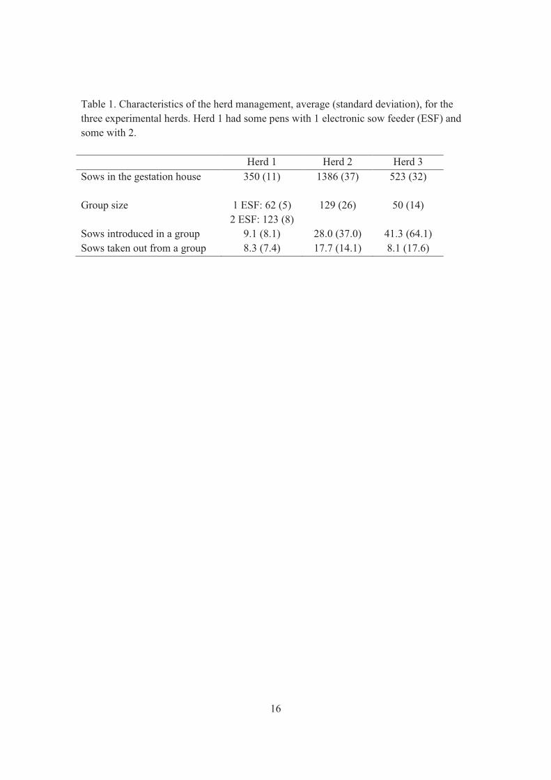
Other characteristics of herd management for the three herds are shown in Table 1.

The number of sows introduced per group was generally a function of the herd size. In

herd 3, with static groups, the number of sows introduced and taken out should in

principle be equal to the group size; in practice, however, this number is reduced due to

frequent movements of individual sows that return to oestrus or are ill. In herds 1 and 2,

with dynamic groups, sows may be taken in or out at any time.

2.1.2. Information collected by ESF

A central computer recorded visits at the ESF for the individual sows. All herds were

equipped with ESF from SKIOLD Echberg A/S (Ikast, Denmark) starting daily feeding

cycle at 17:00, 22:00 and 21:30 for herds 1, 2 and 3, respectively. In all herds, the

duration of a feeding cycle was 24 hours; for herd 1 and 2, the ESF was closed 5 and 4

hours, respectively, before the start of a new feeding cycle. Table 2 presents the

characteristics of the use of the ESF for the three herds. The average use of the ESF was

stable from one herd to the other, but a large intra-herd variation was observed.

For all herds, the feed energy value was 0.95-1.05 FUp.kg-1

of dry feed (Feed Units, pigs:

1 FUp = 7.380 MJ net energy), and water was available in a bowl adjacent the feed bowl.

Transfer from a part of a daily ration not eaten did not exceed 1 kg from one day to

another.

2.1.3. Individual control of oestrus and health status

For the purpose of implementing a detection method for oestrus, lameness and other

health disorders, these three conditions were observed daily for each individual sow by

the herd employees: Back Pressure Test (Willemse and Boender, 1966) was performed to

detect oestrus and visual observations were carried out for identifying lameness and other

health disorders. Identification of a sow presenting one of these conditions was recorded

when the individual was at the ESF or by applying an electronic reading to the individual

ear tag. Every second week, a technician visited each of the three herds in order to ensure

the registration quality of the observations. Each ESF was checked every two months.

Registration was also performed each time a subgroup of sows entered the group, left the

group or when subgroups entered and left a group the same day.

2.2. Modeling of the individual eating behaviour

4

The modeling of the eating behaviour and the detection method were implemented in the

software R (R Development Core Team, 2005).

2.2.1. Definition of the response variable

The individual eating rank was selected as the response variable: it includes the order in

which sows enter the ESF, the group size, and the start of the daily feeding cycle.

From the starting time of the daily feeding cycle at day t, the order, oit, of sow i visiting

the ESF, and eating more than 300 g, was calculated. Afterwards, the relative eating rank

o*it (0 < o*it < 1) was calculated as:

1

*

+=

t

it

itN

oo (1)

where Nt is the total number of sows in the group on day t. To obtain an approximately

normal distribution, the individual eating rank was logistically transformed as:

÷÷ø

öççè

æ

-+=÷÷ø

öççè

æ

-=

itt

it

it

it

itoN

o

o

oO

1log

1log

*

*

(2)

When a sow had not eaten at the end of a daily feeding cycle, the individual eating rank

oit was set to Nt, so that Oit = log(Nt). From (2) it is apparent that a sow eating first

receives the smallest Oit value, while a sow eating last (or not at all) receives the largest

Oit value. Time series of daily eating ranks were generated for each experimental sow, for

their entire gestating period. Since only one sow is modeled at a time, the index i for sow

is omitted in the rest of the paper.

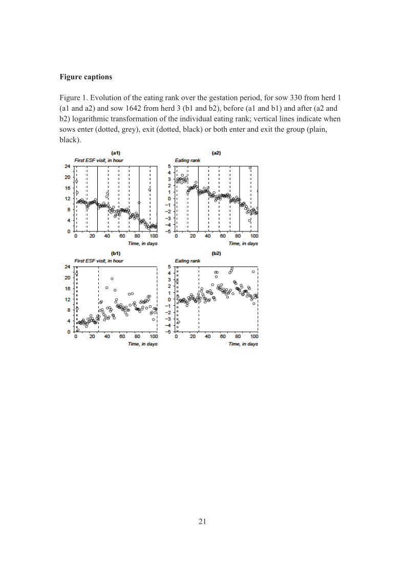
Figure 1 shows the development of the eating rank through a gestation period, both

before (a1 and b1) and after (a2 and b2) logarithmic transformation; it is seen that the

logarithmic transformation increases the stability of the variable over time. Figure 1 (a2)

shows a pattern characteristic of the dynamic groups, as in herd 1 and 2: sows presenting

a low eating rank had the opportunity to increase their rank when sows with higher rank

exit the group. On the other hand, Figure 1 (b2) illustrates that a sow in a static group, as

in herd 3, maintained a relatively constant eating rank over a longer period of time.

2.2.2. Model design

The individual eating rank was modeled using a Dynamic Linear Model (DLM) as

described by West and Harrison (1997). The general DLM is represented as a set of two

equations. The observation equation (3) defines the sampling distribution for the

observation Ot conditional on a state vector θt. The system equation (4) defines the time

5

evolution of the state vector θt. The matrices and state vector are defined in (5): Ft is

called the design matrix and Gt is called the system matrix; θt consists of a set of

parameters describing the model level (µt) and growth (βt) at time t. The error sequences

νt and ωt are assumed internally and mutually independent.

,tt

T

tt FO uq += ),(~ VONtu (3)

,1 tttt G wqq += - ),(~ WONtw (4)

÷÷ø

öççè

æ=

0

1tF ÷÷

ø

öççè

æ=

10

11tG ÷÷

ø

öççè

æ=

t

t

t bm

q (5)

The DLM combined with a Kalman Filter (KF) (Kalman, 1960) estimates the underlying

state vector θt by its mean vector mt and its variance-covariance matrix Ct (the model

variance) given all previous observations O1, . . .Ot of the transformed eating rank. Thus,

the conditional distribution of θt is

( ) ),(~,,| 1 tttt CmNOO Kq (6)

The updating equations of the KF used for stepwise calculation of mt and Ct are found in

West and Harrison (1997). Applications of the KF have been described previously e.g. in

Thysen (1993), de Mol et al. (1999) or Madsen et al. (2005).

The observational variance (V) depends on the accuracy of the measurements by the ESF;

this accuracy being unknown, V is assumed unknown and constant over time. The

evolution variance (Wt) is estimated using a discount factor δ. For each step t, the system

variance Wt is defined as a fixed proportion of the model variance Ct, such as:

T

tttt GCGP += -1 (7)

tt PWdd-

=1

(8)

The model is initialized by means of reference analysis: the first observations of the time

series are used to estimate the posterior distributions after a first period. Missing

observations may occur 1) because a sow did not visit the feeding station during a feeding

cycle or 2) because of technical problems at the ESF. As mentioned in Section 4.1, when

a sow was not registered at the ESF during a feeding cycle, the value of the response

variable was set to: Ot = log(Nt). In the case of a missing value due to technical problems,

the posterior distributions were set equal to the priors, so that on day t, the forecast errors

from the model et = Ot−ft, i.e. difference between the observation and the model forecast

ft, equal zero.

6

External information was included in the model: a model intervention was performed

each time a subgroup entered or left a group or both. For that purpose, the evolution

variance was increased by setting a lower discounting value at the day of intervention, so

that the model adapted more rapidly to the new observation (West and Harrison, 1997,

chap. 11).

2.2.3. Estimation of the evolution variance

The estimation of the discount factor (and thus the evolution variance, Wt) was based on

time series of eating rank from 300 sows (100 sows in each of the three herds), which

satisfied the following criteria:

• The sows were inserted in the group maximum 10 days after mating

• The sows stayed in the same group during the entire gestating period

• The sows were registered at the ESF for a minimum of 90 days

• The sows were neither observed in oestrus nor treated for lameness/disease(s) during

the period

For practical modeling, discount factors in the range of 0.8 to 1 are usually suggested

(West and Harrison, 1997). For the purpose of intervention however the model must be

able to rapidly adapt to the new observation. For a group of sows, the discount factors

used when a subgroup is inserted (δin), taken out (δout) or both (δin|out) must have the

possibility to reach lower values than the one used without intervention. Thus, in total, 4

discount factors (δ, δin, δout, δin|out) must be estimated.

The principle behind the estimation is to find the combination of discount factors

minimizing the MSE, i.e. the mean sum of squares of the forecast errors et of the model.

In practice, δ was varied in the range [0.8, 1.0] by steps of 0.001, while δin, δout and δin|out

are varied in the range [0.008, 0.8] by steps of 0.088. In total, this leads to 200,000

combinations of values for δ, δin, δout and δin|out. Since we have 100 sows in each of the

three herds, it means that the estimation procedure involves calculation of forecast errors

for 60 million time series. Table 3 shows the values of the optimized discount factors for

the three herds.

When subgroups both enter and exit a group the same day, the value of the intervention

discounting (δin|out) is similar to the discount factor used in normal conditions (δ), i.e. for

the days without group mixing (δ). This may be explained by the fact that the entering

subgroup took the place of the subgroup leaving the group.

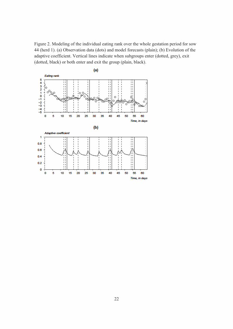
Figure 2 (a) shows the time series of observations (dots) for the individual eating rank of

sow number 44 (herd 1) and the model forecasts (plain) for the whole gestation period.

7

Vertical lines indicate when subgroups are inserted, or exit a group. Figure 2 (b) shows

the evolution of the adaptive coefficient of the DLM (West and Harrison, 1997, p. 38, 42)

at the days of intervention: the increase of the adaptive coefficient at the intervention

days indicates that the new observation is given more weight; the evolution variance is

increased by means of a smaller discounting, which allows the model to adapt quicker to

the new observation.

2.3. Detection method

The detection method consists in applying a V-mask (Montgomery, 1997) on the

cumulative sum (cusum) of the forecast errors from the model et, standardized with

respect to their variance Qt, such as ut = et/√Qt. The cusum, ct, of the standardized errors

ut is calculated as:

å=

=t

t

tt uc1

(9)

In normal conditions, the standardized forecast errors are randomly distributed around

zero. It is expected that when a sow presents a specific condition (oestrus, lameness or

other health disorders), the deviations between the model forecasts and the observations

become wider, so that the cusum tends to drift upwards or downwards. The next section

presents the method implemented to catch these deviations.

2.3.1. The V-mask

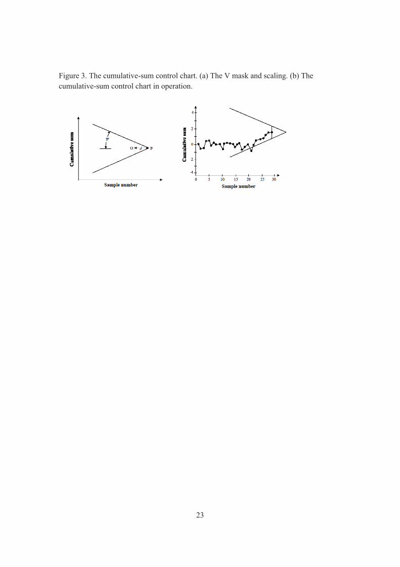
Figure 3 shows a typical V-mask. The V-mask is directly applied on the cusum with the

point O on the last value of ct and the line OP parallel to the horizontal axis. The V-mask

is applied to each new point on the cusum chart and the arms extend backward to the

origin. If all the previous cumulative sums, c1, c2, . . . , ct−1 lie within the two arms of the

V-mask, the process is considered to be ’in-control’; if any of the cumulative sums lies

outside the arms of the mask, the process is considered ’out-of-control’ and an alarm is

given; the value of the cusum is reset to zero each time an alarm is given.

The performance of the V-mask is determined by the lead distance d and the angle Ψ

(Figure 3 (a)). The parameters are estimated as:

÷ø

öçè

æ D=Y -

At

2tan 1 and ÷

ø

öçè

æ -÷ø

öçè

æ=ab

d1

ln2

2d (10)

where α is the probability of detecting a shift when the process is in control (false

positive) and β is the probability of not detecting a shift (false negative) of size δ. An

implementation of the V-mask is presented in Madsen and Kristensen (2005); the authors

8

suggest the following values: α = 0.01, β = 0.01, Δ = 1.5 and A = 1, which imply a lead

distance d » 4 and an angle Ψ = 37o.

2.3.2. Optimization of V-mask parameters

The detection method aims at producing alarms for sows presenting 1) oestrus, 2)

lameness and 3) other health disorders. Recordings of these respective states at the herds

provide days of reference for optimizing the V-mask parameters; the optimization is

based on times series from 300 sows chosen at random, but including individuals

presenting both oestrus, lameness or other health disorders.

The initial parameters are set as in Madsen and Kristensen (2005); only the parameters Δ

and A are optimized. Different values for Δ and A are tested, allowing values of d in the

range [1,9] and Ψ in [24o, 44

o]. An alarm from the V-mask is classified as True Positive

(TP) when it occurs during the following reference periods:

• For oestrus: from 3 days before, to 1 day after the observation

• For lameness: from 6 days before, to the day of observation

• For other health disorders: from 3 days before, to 3 days after the observation

An alarm produced outside these reference periods is considered as False Positive (FP). A

reference period when no alarm is given is considered as False Negative (FN), and a

period with no recording and no alarm is classified as True Negative (TN).

The criteria selected for assessing the method performance were sensitivity, specificity

and error rate (Cornou, 2006): sensitivity = TP/(TP+FN); specificity = TN/(TN+FP);

error rate = FP/(FN+TP). For practical application, it was assumed that monitoring the

three states would require that the detection method helps detecting at least 50% of the

sows presenting the various conditions. Therefore, the V-mask parameters were

optimized so that the sensitivity is at least 50% and the number of FP is minimum.

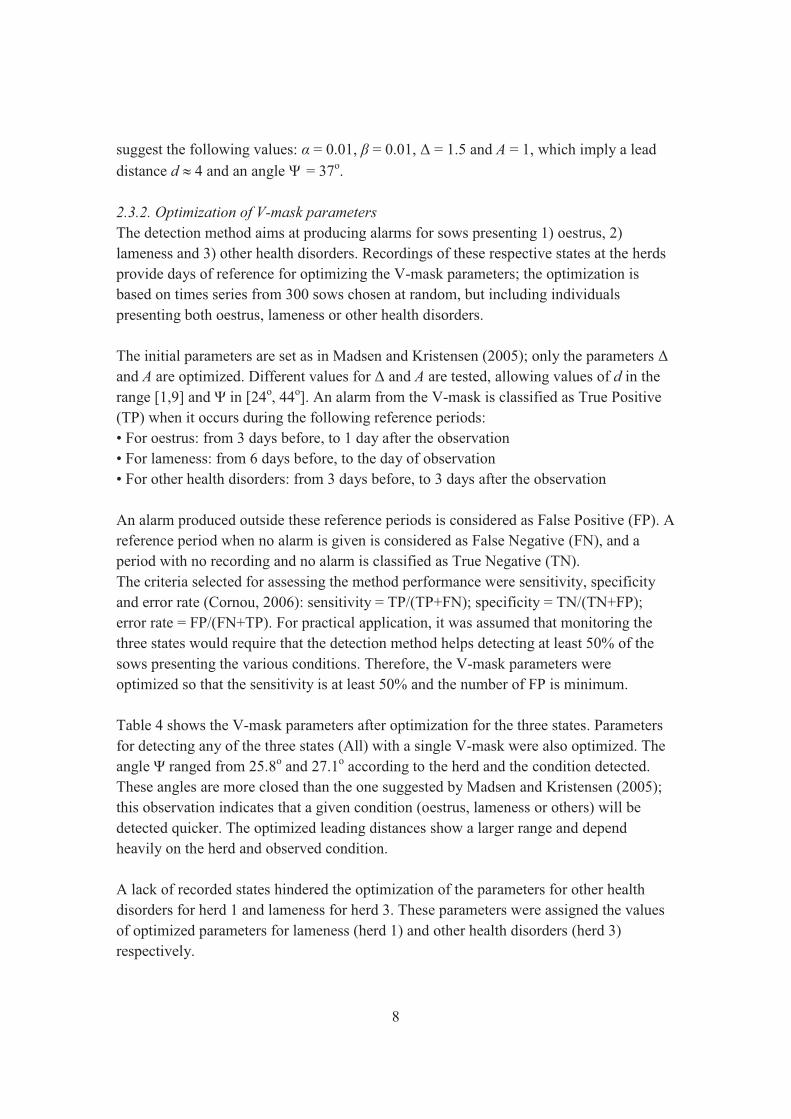
Table 4 shows the V-mask parameters after optimization for the three states. Parameters

for detecting any of the three states (All) with a single V-mask were also optimized. The

angle Ψ ranged from 25.8o and 27.1

o according to the herd and the condition detected.

These angles are more closed than the one suggested by Madsen and Kristensen (2005);

this observation indicates that a given condition (oestrus, lameness or others) will be

detected quicker. The optimized leading distances show a larger range and depend

heavily on the herd and observed condition.

A lack of recorded states hindered the optimization of the parameters for other health

disorders for herd 1 and lameness for herd 3. These parameters were assigned the values

of optimized parameters for lameness (herd 1) and other health disorders (herd 3)

respectively.

9

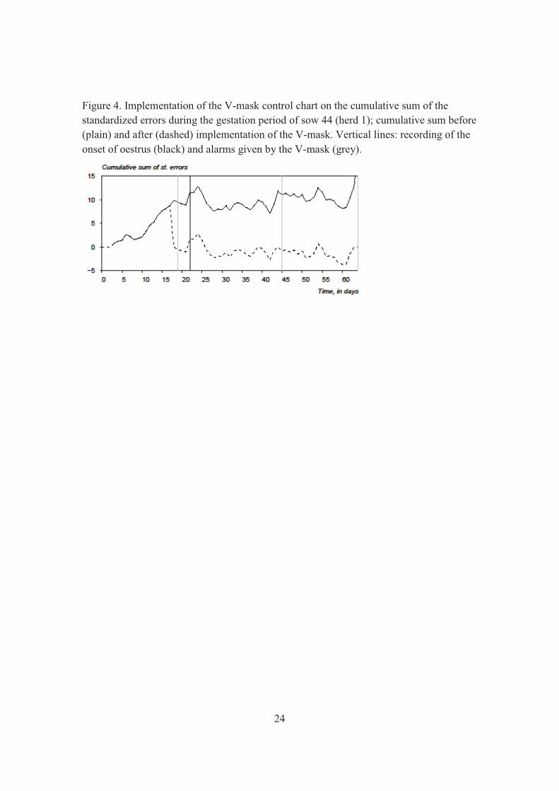
Figure 4 illustrates the implementation of the detection method for sow 44 (see also

Figure 2). The alarms catch abrupt drifts of the cusum, i.e. sudden wide deviations

between observations and forecasts from the model; the value of the cusum is reset to

zero after each alarm given by the V-mask. A first alarm (day 19) is produced three days

before the sow is observed in oestrus (day 22), and afterwards at day 45, 64 and 65.

3. Results

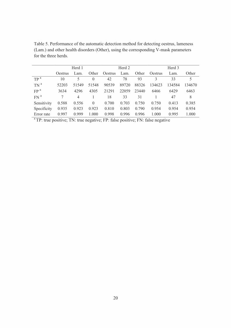
Table 5 shows the performance of the detection method for detecting oestrus, lameness

and other health disorders for the three herds; the total number of days monitored are

55851, 111891 and 141094, respectively, for herds 1, 2 and 3. Each state was detected

using the according V-mask parameters (Table 4) and each time series was modeled

using intervention discounting if relevant (Table 3).

Results indicate that sensitivity ranged from 59% to 75% for oestrus detection, from 41%

to 70% for lameness and from 0% to 75% for detecting other health disorders. To put

these results in perspective, alarms provided by the detection methods are compared to

alarms given when the list of sows that have not eaten is used. Using the lists of sows in

herds 1, 2 and 3, the sensitivity for oestrus detection is 9%, 20% and 50% (less than 5

observations), 39%, 32% and 22% for lameness detection and 71% (less than five

observations) 34% and 16% for detecting other health disorders.

The results in terms of sensitivity are generally higher for the detection method developed

here than when the list of sows is used. The major drawback of the detection method is a

large number of false alarms, which is higher than false alarms provided by the list of

sows: for oestrus detection, the number of false positives observed in herds 1, 2 and 3 is

3634, 21291 and 6466, vs. 1354, 6884 and 3609 when the list of sows was used.

The use of a single V-mask for detecting the three conditions (parameters All in Table 4)

was tested for the three herds. A Pearson’s Chi-square test was made to assess whether

the performances differ compared to the use of each states’ respective V-mask

parameters. For herd 3 sensitivity, specificity and error rate did not differ significantly.

For herd 1, only specificity was significantly different, for the three conditions (p <

0.001). For herd 2, however, only sensitivity and error rate for oestrus detection were

non-significant; the other results differ (p < 0.001). The use of a single V-mask for

detection of the three conditions does not appear relevant; only half the performances

were similar (non significant) when the two methods are compared.

4. Discussion

10

A method is implemented for detecting oestrus, lameness and other health disorders for

group housed sows fed by ESF. The individual eating rank is modeled using a dynamic

linear model; deviations between the model forecast and the observations are monitored

using a V-mask control chart. After optimization of the V-mask parameters, specific

alarms are given for oestrus, lameness and other health disorders.

Results indicate that the detection method allows detection of sows in oestrus with a

sensitivity ranging from 59 to 75%. Compared to other results obtained with either the list

of sows that have not eaten obtained by the ESF (currently the only kind of alarm system

for the farmer) or with a Multi Process Kalman filter (MPKF) as tested by Søllested

(2001), the performance of the automatic detection method developed in this paper

appears satisfying; the sensitivity for these other methods was 9 to 20%, and below 2%

respectively.

However, the number of false alarms given by the detection method was too high. A

possible explanation for the high number of false alarms is the fact that oestrus is a rare

event to monitor: during the implementation of the method in the three herds, only 81

sows showed oestrus, out of the 308836 days of monitoring. Suggestions for improving

the results for automatic oestrus detection are: 1) a reduction of the period for automatic

oestrus detection, as implemented for cows (de Mol et al., 1997). For practical

application, information from ultrasound scanning performed for diagnosing pregnancy

(24 to 38 days after mating) could be included in the model; considering that a sow

cannot be in oestrus the first 14 days after mating (day 0), the period for automatic

oestrus detection could be limited from day 14 to day 38; only sows with a doubtful

pregnancy test should be automatically monitored until a new pregnancy test is

performed. Another suggestion for improving automated oestrus detection would be 2) to

include a sensitive period in the detection model, as done in Søllested (2001), where the

likelihood of a sow being in oestrus was 12.5 greater in the interval day 18-22. To assess

whether this suggestion would improve the results, three sensitive periods were tested:

day 21, day 20-22 and day 19-23. Due to a too low number of sows registered as in

oestrus during these periods, only herd 2 was tested: results indicate that the error rate

was reduced by 0.3% only. The sows registered by the herd’s employees as being in

oestrus were: 5, 15 and 25%, for the three periods. Søllested (2001) indicates that in

normal conditions, 80% of the sows to be mated should be included in the sensitive

period day 18-22; it can therefore be questioned whether all sows showing oestrus were

correctly registered. More reliable reference days should be used in order to improve

accuracy of the detection method; hormonal sampling (progesterone test for instance)

may be used to confirm that ovulation has occurred.

11

The detection method for lameness and other health disorders shows a sensitivity ranging

from 41 to 70%, compared to 22 to 39% when the list of sows from the ESF was used as

alarm. As for oestrus detection, a major drawback of the method is a too high number of

false alarms. A suggestion for reducing the number of false alarms is to broaden the

reference periods in which sows with lameness and other health disorders were observed

at the herd; the reference period used in this experiment was from 6 days before up to the

day of observation (lameness), and from 3 days before to 3 days after the observation

(other health disorders). The justification for the choice of the reference period for other

health disorders was that individual eating behaviour may not be influenced so drastically

in the case of, for instance, vulva biting. For dairy cows, de Mol et al. (1997) suggest a

reference period of 7 days before to 7 days after the observation of other health problems

than mastitis; a broader reference period should be tested in attempt to improve the

method’s performance. Besides, it can be argued that a sow presenting health disorders is

expected to decrease in eating rank; detection of deviations in one side only, i.e.

downward drift of the eating rank, may help reduce the number of false positives. A

control chart such a Tabular Cusum (Montgomery, 1997), which allows monitoring

separately upwards and downwards drifts of model deviations, may be used for this

purpose.

In this study, the average daily visits per sow indicate a stable eating pattern: 3.0, 2.6 and

3.2 for herds 1, 2 and 3, compared to 7.2 reported by Søllested (2001). The high

percentage of sows eating their entire daily ration at the first visit (95.3, 93.5 and 79.5%)

is in accordance with Eddison and Roberts (1995); these last authors reported that 79% of

all sows ate more than 95% of their daily feeding ration at their first visit at the ESF. This

further supported the argument of excluding the number of visits at the ESF for modeling

individual eating behaviour.

The detection method suggested in this article is based on monitoring the individual

eating rank of group housed sows. The eating rank is selected due to its characteristic

stability over a short period of time (Edwards et al., 1988; Bressers, 1993) as well as its

interest in directly including information about the group size; this information is

modeled in a single time series for each sow. An alternative model is to use both

information (eating rank and the group size) in two separate time series, which are

aggregated in a multivariate model based on covariances. However, the complexity of

this kind of multivariate model as well as the variation of group sizes over time in

dynamic groups limit its interest for practical application. On the other hand, a model

including information about the eating hierarchy of an entire group would allow better

predictions within subgroups; information about the age and size of sows could be used

for the purpose (Hunter et al., 1988; Connell et al., 2003).

12

In the DLM presented in this article, model interventions are performed in order to

include information about insertion and/or exclusion of subgroups within a group.

Intervention consists in temporarily decreasing the value of the discount factor, to allow

the model to adapt quicker to the new observation, and limit a drift of the cumulative sum

of forecast errors responsible for alarms. Intervention is performed the same day as the

structure of a group was modified; Arey and Edwards (1998) cite Oldigs et al. (1992) and

Putten and de Burgwal (1990), who report that the number of aggressions after group

mixing stabilizes 3 and 10 days after introduction of new sows in a group, respectively .

The duration of intervention discounting, limited to a single day in this experiment, may

have prevented observation of effects of group mixing: even though all herds were found

to be affected when a subgroup exits a group, only herd 2 was affected by insertion of a

subgroup. Therefore, a longer period of intervention should be tested; however, a too

long intervention risks covering possible changes in individual eating rank. For instance,

lameness caused by fights for rank attribution may not be detected because of the faster

model adaptation in this intervention period.

To improve both the sensitivity and the specificity of the detection method, it is suggested

to include a larger number of variables. For dairy cows, de Mol et al. (1997) suggest a

multivariate model including five response variables for detecting oestrus and health

disorders. For group housed sows fed by ESF, the daily feed consumption could provide

information both for detecting oestrus and health disorders (Søllested, 2001; Forbes,

1995; Friend, 1973); ear based temperature (Bressers et al., 1994; Geers et al., 1996) or

body activity (Bressers et al., 1993b; Cornou and Heiskanen, 2007) are also potential

additional variables. Tasch and Rajkondawar (2004) and Pastell et al. (2006) present a

method for detecting lameness for dairy cows, by measuring leg pressure using force

sensors; such a method may also be considered for detecting lameness for group housed

sows, for instance, when sows are at the ESF. An alternative model, where detection of

abnormal states is built-in is the Multi Process Kalman Filter (MPKF) (Thysen, 1993;

Søllested, 2001); a MPKF consists of parallel models, each with specific parameters, for

a given time series; one of the models, which refers to outliers, can be used to produce

alarms, instead of the V-mask, for instance. A drawback of this kind of model is that it is

based on the last observation only, and may not be apt to detect a gradual change of the

individual eating behaviour, as it may occur for oestrus or health problems; this may

explain the very low sensitivity reported by Søllested (2001).

5. Conclusion

The detection method suggested in this article shows a sensitivity that ranges from 39 to

75% according to the condition detected, i.e. oestrus, lameness or other health disorders.

Results indicate that the detection method performs generally better than when the list of

sows that have not eaten (provided by the ESF and only current tool available to the

13

farmer) is used as alarms. The major drawback of the detection method for the three

conditions is a too high number of false alarms. Measurement of the individual eating

rank appears a relevant response variable, since it includes information on the group size.

However, models including covariance may help to model more accurately interactions

between individual and group eating rank. To improve the performance of the method, it

is suggested to reduce the monitoring period (for oestrus) and to include more variables

such as body activity or temperature (for all conditions).

6. Acknowledgements

The authors gratefully acknowledge the employees of the production herds and the

Danish Pig Production for the data collection.

References

Arey, D. S., 1999. Time course for the formation and disruption of social organization in

group-housed sows. Appl. Anim. Behav. Sci. 62 (2-3), 199–207.

Arey, D. S., Edwards, S., 1998. Factors influencing aggression between sows after

mixing and consequences for welfare and production. Livest. Prod. Sci. 56, 61–70.

Bressers, H. P. M., 1993. Monitoring individual sows in group housing. Possibilities for

automation. Rappoort Instituut voor Veeteeltkundig Onderzoek "Schoonoord" (B-396),

pp. 135.

Bressers, H. P. M., Brake, J. H. A. T., Engel, B., Noordhuizen, J. P. T. M., 1993a.

Feeding order of sows at an individual electronic feed station in a dynamic group housing

system. Appl. Anim. Behav. Sci. 35, 123–134.

Bressers, H. P. M., Cats, T., te Brake, J. H. A., Jansen, M. B., Noordhuizen, J., 1993b.

Oestrus-associated physical activity in group-housed sows. Ph.D. thesis, Wageningen

Agricultural University, Departement of Animal Husbandry, P.O. Box 338 6700 AH

Wageningen.

Bressers, H. P. M., te Brake, J. H. A., Jansen, M. B., Nijenhuis, P. J., Noordhuizen, J. P.

T. M., 1994. Monitoring individual sows: radiotelemetrically recorded ear base

temperature changes around farrowing. Livest. Prod. Sci. 37 (3), 353–361.

Connell, N. E. O., Beattie, V. E., Moss, B., 2003. Influence of social status on the welfare

of sows in static and dynamic groups. Anim. Welf. 12, 239–249.

Cornou, C., 2006. Automated oestrus detection methods in group housed sows: Review

of the current methods and perspectives for development. Livest. Sci. 105, 1–11.

Cornou, C., Heiskanen, T., 2007. Automated oestrus detection method for group housed

sows using acceleration measurements. Proceedings of the 3ECPLF. Skiathos, Greece, 3-

6 June 2007, pp. 211-217.

de Mol, R. M., Keen, A., Kroeze, G. H., Achten, J. M. F. H., April 1999. Description of a

detection model for oestrus and diseases in dairy cattle based on time series analysis

combined with a kalman filter. Comput. Electron. Agric. 22 (2-3), 171–185.

14

de Mol, R. M., Kroeze, G. H., Achten, J. M. F. H., Maatje, K., Rossing, W., 1997.

Results of a multivariate approach to automated oestrus and mastitis detection. Livest.

Prod. Sci. 48, 219–229.

Eddison, J., Roberts, N., 1995. Variability in feeding behaviour of group-housed sows

using electronic feeders. Anim. Sci. 60, 307–314.

Edwards, S., 21-24 August 2000. Alternative housing for dry sows: system studies or

component analyses? improving health and welfare in animal production. In: Proceedings

of sessions of the EAAP Commission on Animal Management and Health. The Hague.

Netherlands, pp. 99–107.

Edwards, S., Armsby, A., Large, J., 1988. Effects of feed station design on the behaviour

of group housed sows using an individual feeding system. Livest. Prod. Sci. 18, 511–522.

Forbes, J. M., 1995. Voluntary food intake and diet selection in farms animals. CAB

international, Wallingford, Oxon OX10DE, UK.

Friend, D.W., 1973. Self-selection of feeds and water by unbred gilts. J. Anim. Sci. 5,

1137–1141.

Geers, R., Janssens, S., Jourquin, J., Goedseels, V., Goossens, K., Ville, H., Vandoorne,

N., 1996. Measurement of ear base temperature as a tool for sow management. Trans.

ASAE 39 (2), 655–659.

Hunter, E., Broom, D., Edwards, S., Sibly, R., 1988. Social hierarchy and feeder access in

a group of 20 sows using a computer-controlled feeder. Anim. Prod. 47, 139–148.

Jensen, K., Sørensen, L., Bertelsen, D., Pedersen, A., Jørgensen, E., Nielsen, N.,

Vestergaard, 2000. Management factors affecting activity and aggression in dynamic

group housing systems with electronic sow feeding: a field trial. Anim. Sci. 71, 635–545.

Kalman, R., 1960. A new approach to linear filtering and prediction problems. J. Basic

Engin. 82, 35–45.

Madsen, T., Andersen, S., Kristensen, A., 2005. Modeling the drinking pattern of young

pigs using a state space model. Comput. Electron. Agric. 48, 39–62.

Madsen, T., Kristensen, A., 2005. A model for monitoring the condition of young pigs by

their drinking behaviour. Comput. Electron. Agric. 48, 138–154.

Montgomery, D., 1997. Introduction to Statistical Quality Control, 3rd Edition. John

Wiley and Sons, USA.

Oldigs, B., Schlichting, M., Ernst, T., November 1992. Trial on the grouping of sows. In:

Proceedings of the 23rd international conference on applied ethology in livestock. No.

351. Freiburg im Breisgau, Germany, pp. 109–120.

Pastell, M., Aisla, A., Hautala, M., Ahokas, J., Poikalainen, V., Praks, J., 2006.

Measuring lameness in dairy cattle using force sensors. In: World Congress: Agricultural

Engineering for a BetterWorld. Book of Abstracts. Bonn, Germany, pp. 525–526.

15

Putten, G. V., de Burgwal, J. V., 1990. Pig breeding in phases. In: Electronic

identification in pig production. Proceedings of an international symposium, Rase,

Stoneleigh. pp. 115–120.

R Development Core Team, 2005. R: A language and environment for statistical

computing. R Foundation for Statistical Computing, Vienna, Austria.

Søllested, T., 2001. Automatic oestrus detection by modelling eating behaviour of group-

housed sows in electronic sow feeding system. Thesis/dissertation.

Spoolder, H., burbidge, J., Edeards, S., Lawrence, A., Simmins, P., 1997. Effects of food

level on performance and behaviour of sows in a dynamic group-housing system with

electronic feeding. Anim. Sci. 65, 473–482.

Tasch, U., Rajkondawar, P. G., 2004. The development of a softseparator for a lameness

diagnostic system. Comput. Electron. Agric. 44, 239–245.

Thysen, I., 1993. Monitoring bulk tank somatic cell counts by a multi-process kalman

filter. Acta Agric. Scand. Sect. A. Animal Sci. (43), 58–64.

West, M., Harrison, J., 1997. Bayesian Forecasting and Dynamic Models, 2nd Edition.

Springer, New York, USA.

Whittemore, C., 1998. The science and practice of pig production, 2nd Edition. Oxford.

Willemse, A.H., Boender, J., 1966. A quantitative and qualitative analysis of oestrus in

gilts. Tijdschr. Diergeneesk. 91 (6), 349-362.

16

Table 1. Characteristics of the herd management, average (standard deviation), for the

three experimental herds. Herd 1 had some pens with 1 electronic sow feeder (ESF) and

some with 2.

Herd 1 Herd 2 Herd 3

Sows in the gestation house 350 (11) 1386 (37) 523 (32)

Group size

1 ESF: 62 (5)

2 ESF: 123 (8)

129 (26) 50 (14)

Sows introduced in a group 9.1 (8.1) 28.0 (37.0) 41.3 (64.1)

Sows taken out from a group 8.3 (7.4) 17.7 (14.1) 8.1 (17.6)

17

Table 2. Use of the electronic sow feeders (ESF), average (standard deviation), for the

three experimental herds.

Herd 1 Herd 2 Herd 3

Sows per ESF per day 61.6 (4.32) 64.7 (13.2) 59.7 (21.0)

Visits per ESF per day 186.4 (52.2) 171.0 (49.4) 191.5 (59.0)

Feeding visits per ESF per day 63.0 (6.7) 67.0 (15.5) 59.7 (21.0)

Perc. of sows eating their

entire ration at first visit

95.3 (6.4) 93.5 (13.8) 79.5 (20.5)

18

Table 3. Value of the optimized discount factors (δ) and respective mean squared errors

(MSE) for the three herds.

Herd 1 Herd 2 Herd 3

δin 0.813 0.204 0.906

δout 0.461 0.644 0.114

δin|out 0.813 0.996 0.906

δ 0.813 0.996 0.906

MSE 0.113 0.763 0.790

19

Table 4. Estimated V-mask parameters used to detect the three respective conditions and

any of the three conditions (All), for the three herds.

Herd 1 Herd 2 Herd 3

Ψ d Ψ d Ψ d

Oestrus 25.8 3.2 25.8 1.7 25.8 4.7

Lameness 27.1 4.1 25.8 6.4 - -

Other - - 25.8 4.7 25.8 4.7

All 25.8 1.5 25.8 3.6 25.8 4.7

20

Table 5. Performance of the automatic detection method for detecting oestrus, lameness

(Lam.) and other health disorders (Other), using the corresponding V-mask parameters

for the three herds.

Herd 1 Herd 2 Herd 3

Oestrus Lam. Other Oestrus Lam. Other Oestrus Lam. Other

TP a 10 5 0 42 78 93 3 33 5

TN a 52203 51549 51548 90539 89720 88326 134623 134584 134670

FP a 3634 4296 4305 21291 22059 23440 6466 6429 6463

FN a 7 4 1 18 33 31 1 47 8

Sensitivity 0.588 0.556 0 0.700 0.703 0.750 0.750 0.413 0.385

Specificity 0.935 0.923 0.923 0.810 0.803 0.790 0.954 0.954 0.954

Error rate 0.997 0.999 1.000 0.998 0.996 0.996 1.000 0.995 1.000 a TP: true positive; TN: true negative; FP: false positive; FN: false negative

21

Figure captions

Figure 1. Evolution of the eating rank over the gestation period, for sow 330 from herd 1

(a1 and a2) and sow 1642 from herd 3 (b1 and b2), before (a1 and b1) and after (a2 and

b2) logarithmic transformation of the individual eating rank; vertical lines indicate when

sows enter (dotted, grey), exit (dotted, black) or both enter and exit the group (plain,

black).

22

Figure 2. Modeling of the individual eating rank over the whole gestation period for sow

44 (herd 1). (a) Observation data (dots) and model forecasts (plain); (b) Evolution of the

adaptive coefficient. Vertical lines indicate when subgroups enter (dotted, grey), exit

(dotted, black) or both enter and exit the group (plain, black).

23

Figure 3. The cumulative-sum control chart. (a) The V mask and scaling. (b) The

cumulative-sum control chart in operation.

24

Figure 4. Implementation of the V-mask control chart on the cumulative sum of the

standardized errors during the gestation period of sow 44 (herd 1); cumulative sum before

(plain) and after (dashed) implementation of the V-mask. Vertical lines: recording of the

onset of oestrus (black) and alarms given by the V-mask (grey).