Automatic Control of the 30 MWe SEGS VI

Parabolic Trough Plant

by

THORSTEN A. STUETZLE

A thesis submitted in partial fulfillment of the requirements for the degree of

MASTER OF SCIENCE (MECHANICAL ENGINEERING)

at the

UNIVERSITY OF WISCONSIN-MADISON

2002

ii

iii

Abstract

A solar electric generating system (SEGS) can be divided into two major subsystems

(Lippke, 1995): a solar collector field and a conventional Clausius-Rankine cycle with a

turbine-generator. For the 30 MWe SEGS VI Parabolic Trough Collector Plant, one task of a

skilled plant operator is to maintain a specified set point of the collector outlet temperature

by adjusting the volume flow rate of the heat transfer fluid circulating through the collectors.

The collector outlet temperature is mainly affected by changes in the sun intensity, by the

collector inlet temperature and by the volume flow rate of the heat transfer fluid. For the

development of next generation SEGS plants and in order to obtain a control algorithm that

approximates an operator’s behaviour, a linear model predictive controller is developed for

use in a plant model. The plant model, which is discussed first in this work, consists of a

model for the parabolic trough collector field and a model for the power plant. The plant

model’s usefulness is evaluated through a comparison between predicted and measured data.

The performance of the controller is evaluated on four different days in 1998. The influence

of the control on the gross output of the plant is examined as well.

iv

v

Acknowledgements

I am very grateful to my advisors, Professor William A. Beckman and Professor John

W. Mitchell, for their guidance and encouragement of my research efforts. In addition, I

would like to thank Professor Sandy Klein for his help with EES during this project.

I am grateful to Professor James B. Rawlings from the Department of Chemical

Engineering who introduced me to Professor Beckman and this project when I attended his

course on model predictive control.

I would like to thank Professor Heisel, Ms. Peik-Stenzel and Dr. Michaelis from the

University of Stuttgart. Their efforts gave me the opportunity to study at the Department of

Mechanical Engineering at the University of Wisconsin-Madison. Thanks to the German

Academic Exchange Service (DAAD) for the financial support during that time. In addition,

I would like to thank Professor Zeitz from the University of Stuttgart for providing great

support to students of Engineering Cybernetics who are studying abroad.

The thesis work was sponsored by Sandia National Laboratories, a multi-program

laboratory operated by Sandia Corporation, a Lockheed Martin Company, for the United

States Department of Energy under Contract DE-AC04-94AL85000. A special thank you to

Scott Jones of Sandia National Laboratories for his assistance during this project.

Many thanks to Professor Tim Shedd, Professor Greg Nellis, and the graduate

students and staff of the Solar Lab for their friendship and help during my stay here.

I would like to thank the international students from the Madison 2001 mailing list for

friendship and joint leisure time activities.

vi

Finally, many thanks to my parents who could always be counted on as a source of

caring and support, even from a distance of about 4000 miles.

vii

Table of Contents Abstract ...................................................................................iii Acknowledgements...................................................................v Table of Contents....................................................................vii List of Figures...........................................................................ix Chapter 1 Introduction..............................................................................1 Chapter 2 Trough Collector Field Model .....................................................5

2.1 Introduction....................................................................................................................5 2.2 Modeling of the Collector..............................................................................................9

2.2.1 Partial Differential Equation for Temperature ......................................................9 2.2.2 Heat Transfer between the Absorber and the HTF .............................................12 2.2.3 Heat Transfer between the Absorber and the Envelope......................................14 2.2.4 Heat Transfer between the Glass Envelope and the Environment......................17 2.2.5 Absorbed Solar Energy .......................................................................................19

2.3 Model Implementation and Simulation Results...........................................................39 2.3.1 Implementation in Digital Machines ..................................................................40 2.3.2 Simulation Results and Model Validation..........................................................42

Chapter 3 Power Plant Model ..................................................................47

3.1 Introduction..................................................................................................................47 3.2 Modeling of the Power Plant .......................................................................................50

3.2.1 Simplifications ....................................................................................................50 3.2.2 Modeling .............................................................................................................54

3.2.2.1 Condensate Pump CP and Feedwater Pump FP ........................................54 3.2.2.2 High-Pressure Turbine HPT 1, HPT 2 and

Low-Pressure Turbine LPT 1, LPT 2, LPT 3 ............................................56 3.2.2.3 Low Pressure Feedwater Heater LPFH......................................................62 3.2.2.4 Deaerator D and Throttle Valve TV 1 .......................................................64 3.2.2.5 High-Pressure Feedwater Heater HPFH....................................................67 3.2.2.6 Condenser C and Throttle Valve TV 2 ......................................................69

viii

3.2.2.7 Heat Exchanger Train HE A and HE B and Reheater RH A and RH B....74 3.2.2.8 Calculation of the Gross Output ................................................................84

3.3 Model Implementation and Simulation Results...........................................................84

Chapter 4 Combined Plant Model.............................................................89 Chapter 5 Linear Model Predictive Control ..............................................95

5.1 Introduction..................................................................................................................95 5.2 The Simplified Model..................................................................................................97 5.3 Models for Linear MPC.............................................................................................103

5.3.1 Model Linearization..........................................................................................107 5.3.2 Discrete-Time Models .......................................................................................121

5.4 The Model Predictive Control Framework ................................................................122 5.4.1 Receding Horizon Regulator Formulation........................................................122 5.4.2 Target Calculation.............................................................................................128 5.4.3 State Estimator ..................................................................................................130

5.5 Controller Implementation and Results .....................................................................132 Chapter 6 Conclusions and Recommendations ......................................141

6.1 Conclusions ................................................................................................................141 6.2 Recommendations ......................................................................................................142

Appendix A Collector Dimensions.............................................................143 Appendix B Nomenclature........................................................................145 References ............................................................................151

ix

List of Figures

Fig. 1.1 Areal view of a SEGS plant .....................................................................................1 Fig. 1.2 Parabolic trough collector of a SEGS plant .............................................................2 Fig. 1.3 Flow diagram of the 30 MWe SEGS VI plant .........................................................3 Fig. 2.1 Layout of the SEGS VI plant ...................................................................................5 Fig. 2.2 Solar collector assembly ..........................................................................................6 Fig. 2.3 Schematic of a heat collection element....................................................................7 Fig. 2.4 Heat transfer of the HCE..........................................................................................8 Fig. 2.5 Schemata of the HCE...............................................................................................9 Fig. 2.6 Emissivity of the absorber vs. temperature ............................................................17 Fig. 2.7 Direct normal radiation at June 20, 1998 and December 16, 1998........................21 Fig. 2.8 North-south tracking ..............................................................................................22 Fig. 2.9 Sun’s coordinates relative to the collector .............................................................23 Fig. 2.10 Celestial sphere showing sun’s declination angle..................................................25 Fig. 2.11 Declination vs. month............................................................................................26 Fig. 2.12 Equation of time.....................................................................................................27 Fig. 2.13 End losses of a trough collector .............................................................................29 Fig. 2.14 Incidence angel modifier vs. angle of incidence....................................................30 Fig. 2.15 Illustration of mutual shading in a multirow collector array .................................32 Fig. 2.16 Mutual collector shading........................................................................................33 Fig. 2.17 Geometric considerations on the collector.............................................................34

x

Fig. 2.18 Optical losses at June 20, 1998 ..............................................................................37 Fig. 2.19 Optical losses at December 16, 1998 .....................................................................38 Fig. 2.20 The collector model as a block ..............................................................................39 Fig. 2.21 Discretization of the HCE......................................................................................41 Fig. 2.22 Measured trough collector field inlet temperature .................................................42 Fig. 2.23 Measured HTF volume flow rate ...........................................................................43 Fig. 2.24 Measured direct normal solar radiation .................................................................43 Fig. 2.25 Measured ambient temperature ..............................................................................43 Fig. 2.26 Measured wind speed.............................................................................................44 Fig. 2.27 Collector model: calculated vs. measured collector outlet temperature, on June 20, 1998 ....................................................................................................45 Fig. 2.28 Collector model: calculated vs. measured collector outlet temperature, on September 19, 1998...........................................................................................45 Fig. 2.29 Collector model: calculated vs. measured collector outlet temperature, on December 16, 1998 ...........................................................................................46 Fig. 2.30 Collector model: calculated vs. measured collector outlet temperature, on December 14, 1998 ...........................................................................................46 Fig. 3.1 The power plant part of SEGS VI ..........................................................................47 Fig. 3.2 Simplification in the power plant structure............................................................51 Fig. 3.3 Simplified power plant structure............................................................................52 Fig. 3.4 T-s-diagram for June 20, 1998, 1.00pm.................................................................53 Fig. 3.5 The power plant model as a block .........................................................................84 Fig. 3.6 Measured expansion vessel temperature................................................................85

xi Fig. 3.7 Measured steam mass flow rate .............................................................................85 Fig. 3.8 Measured cooling water inlet temperature.............................................................86 Fig. 3.9 Power plant: calculated vs. measured collector inlet temperature and gross output, June 20, 1998 .............................................................................86 Fig. 3.10 Power plant: calculated vs. measured collector inlet temperature and gross output, September 19, 1998 ..................................................................87 Fig. 3.11 Power plant: calculated vs. measured collector inlet temperature and gross output, December 16, 1998....................................................................87 Fig. 3.12 Power plant: calculated vs. measured collector inlet temperature and gross output, December 14, 1998....................................................................87 Fig. 4.1 Combinaton of collector model and power plant model........................................89 Fig. 4.2 The combined plant model as a block....................................................................90 Fig. 4.3 Plant model: calculated vs. measured collector outlet temperature and gross output, June 20, 1998 .............................................................................91 Fig. 4.4 Plant model: calculated vs. measured collector outlet temperature and gross output, September 19, 1998 ...................................................................91 Fig. 4.5 Plant model: calculated vs. measured collector outlet temperature and gross output, December 16, 1998....................................................................91 Fig. 4.6 Plant model: calculated vs. measured collector outlet temperature and gross output, December 14, 1998....................................................................92 Fig. 5.1 The MPC controller for the plant model................................................................95 Fig. 5.2 The structure of the simplified model....................................................................98 Fig. 5.3 Simplified model prediction vs. measurement, June 20, 1998 ............................102 Fig. 5.4 Simplified model predicion vs. measurement, December 14, 1998 ....................102 Fig. 5.5 Simplified model: linear vs. nonlinear, June 20, 1998 ........................................118

xii

Fig. 5.6 Simplified model: linear vs. nonlinear, December 14, 1998 ...............................119 Fig. 5.7 Complex model: linear vs. nonlinear ...................................................................120 Fig. 5.8 The receding horizon regulator as a block ...........................................................128 Fig. 5.9 The target calculation as a block..........................................................................129 Fig. 5.10 The state estimator as a block ..............................................................................132 Fig. 5.11 MPC controller structure......................................................................................133 Fig. 5.12 MPC control results, June 20, 1998 .....................................................................134 Fig. 5.13 MPC control results, September 19, 1998 ...........................................................135 Fig. 5.14 MPC control results, December 16, 1998 ............................................................136 Fig. 5.15 MPC control results, December 14, 1998 ............................................................137

1

Chapter 1

Introduction

A solar electric generating system (SEGS), shown in Figure 1.1, refers to a class of solar

energy systems that use parabolic troughs in order to produce electricity from sunlight

(Pilkington, 1996).

Figure 1.1: Areal View of a SEGS Plant

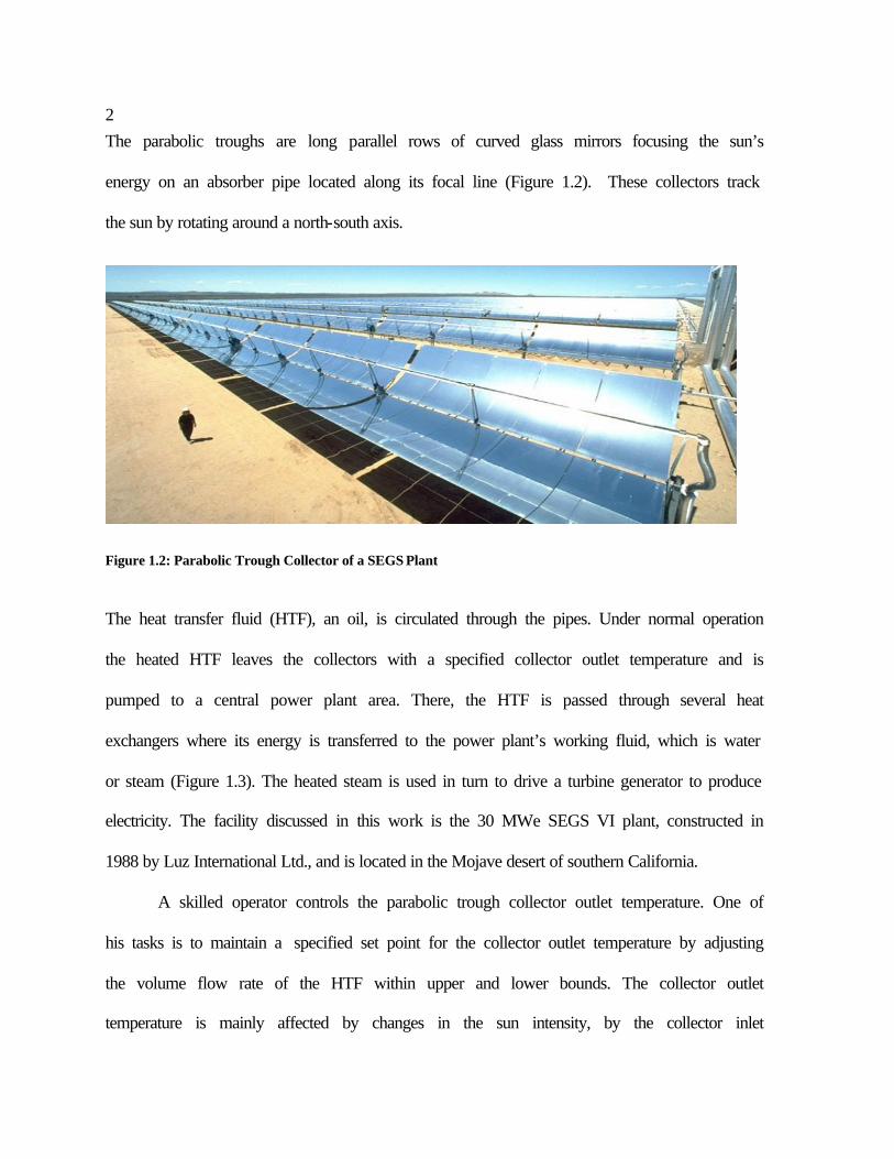
2The parabolic troughs are long parallel rows of curved glass mirrors focusing the sun’s

energy on an absorber pipe located along its focal line (Figure 1.2). These collectors track

the sun by rotating around a north-south axis.

Figure 1.2: Parabolic Trough Collector of a SEGS Plant

The heat transfer fluid (HTF), an oil, is circulated through the pipes. Under normal operation

the heated HTF leaves the collectors with a specified collector outlet temperature and is

pumped to a central power plant area. There, the HTF is passed through several heat

exchangers where its energy is transferred to the power plant’s working fluid, which is water

or steam (Figure 1.3). The heated steam is used in turn to drive a turbine generator to produce

electricity. The facility discussed in this work is the 30 MWe SEGS VI plant, constructed in

1988 by Luz International Ltd., and is located in the Mojave desert of southern California.

A skilled operator controls the parabolic trough collector outlet temperature. One of

his tasks is to maintain a specified set point for the collector outlet temperature by adjusting

the volume flow rate of the HTF within upper and lower bounds. The collector outlet

temperature is mainly affected by changes in the sun intensity, by the collector inlet

3temperature and by the volume flow rate of the HTF. The ambient temperature and the wind

speed also influence the outlet temperature but their influence is small.

Figure 1.3: Flow Diagram of the 30 MWe SEGS VI Plant

Knowledge of the sun’s daily path, observation of clouds and many years of experience and

training give the operator the ability to accomplish his task. But there are limitations on the

performance of a human controller. Thus, for the development of next generation SEGS

plants, it is reasonable to look at automatic controls. In addition, a control algorithm that

approximates an operator’s behavior can be included in simulation models of SEGS plants.

Solar Collector Field

Expansion Vessel

Reheater

Preheater

Steam Generator

Superheater

HTF Pump

~ HP- LP- Turbine

Condenser

Deaerator

HP- Feedwater Heater

LP- Feedwater Heater

Condensate Pump

Feedwater Pump

Generator

4Automatic control of the HTF in a parabolic trough collector through proportional control

has been previously addressed (Schindwolf, 1980). In this study, a linear model predictive

controller is developed for the SEGS VI plant. The essential idea behind model predictive

control (MPC) is to optimize forecasts of process behavior. The forecasting is accomplished

with a process model. Therefore, the model is the essential element of a MPC controller

(Rawlings, 2000). The control strategy considers constraints on both the collector outlet

temperature and the volume flow rate of the HTF.

In this work, the control performance is evaluated through simulations. Consequently

it is very important to obtain an accurate model of the plant on which the controller can be

tested.

The following three chapters deal with the modeling of the plant. From Figure 1.3, it

can be seen that the plant consists of two cycles: the cycle of the HTF through the collector

field, indicated by the orange color, and the power plant cycle, indicated by the blue colors.

In Chapter 2, a trough collector field model is presented. In Chapter 3, a model for the power

plant is proposed. Chapter 4 shows simulation results with the combined model and predicted

and measured data are compared in order to evaluate the model.

Finally, in the last chapter, the model predictive control concept is introduced with a

simplified plant model. The control performance is evaluated through simulations with the

complex plant model from Chapter 4 and compared to the performance of a human

controller. The influence of the control on the gross output of the plant is examined as well.

5

Chapter 2

Trough Collector Field Model

2.1 Introduction The 30 MWe SEGS VI plant is located in the Mojave desert of southern California. The

layout of the plant is shown in Figure 2.1.

Figure 2.1: Layout of the SEGS VI plant

The Figure 2.1 shows the power plant with the solar trough collector field. The solar trough

collector field can be divided into four quadrants. There are three quadrants with 12 solar

trough collectors each and one quadrant with 14 solar trough collectors: for a total of 50 solar

N

Power Plant 1 SCA (Solar Collector Assembly)

A Loop of 16 SCAs = 1 Collector

50 Loops together

397.12 m

6trough collectors. One of these 50 collectors is formed by a loop of 16 solar collector

assemblies (SCA). The cold heat transfer fluid (HTF) flows into the collector loop at one

end, indicated by the blue color in the Figure, is heated up by the absorbed energy of the sun

and leaves the collector at the other end, indicated by the red color. The hot HTF of every

collector merges in a central header, which is connected to the power plant. In the power

plant, the heat energy of the merged hot HTF is used to heat a working fluid, which is water

or steam. After transferring its thermal energy to the power plant, the cold HTF leaves the

power plant in a central header that feeds the 50 collectors in the field with the cold fluid.

There are flow balance valves between the collector loops and the headers. The total length

of one collector is two times 397.12 m. The collectors are single-axis tracking and aligned on

a north-south line, thus tracking the sun from east to west.

Figure 2.2: Solar Collector Assembly

The structure of a part of one SCA is given in Figure 2.2 (Pilkington 1996). The entire SCA

consists of six mirror panels. In Figure 2.2 only two of them are shown. All the SCAs are

Heat Collection Element

Mirror Panel Mirror Panel

Hydraulic Drive System with Controller

Drive Pylon

Intermediate Pylon

V- Truss

Connections, Arms, Bellows, etc.

7controlled by a main process computer, the Field Supervisory Controller (FSC). There is one

drive pylon in the center of each SCA with the FSC controlled hydraulic drive system. The

six mirror panels are held up either by the central drive pylon, intermediate pylons or by

shared pylons between two SCAs or by an end pylon when it is the last SCA in a row. The

length of an entire collector mirror is the length of one mirror panel times the number of

mirror panels in a single collector. The collector mirror length is m6.753=Length . The

low-iron glass parabolic mirrors reflect the solar radiation to the heat collection element

(HCE) that is mounted on the SCA through arms.

The HCE, shown in Figure 2.3, is a cermet-coated, stainless-steel absorber tube,

surrounded by a partially evacuated glass envelope. The HTF flows in the absorber tube.

Figure 2.3: Schematic of a Heat Collection Element

Not shown in Figure 2.3 are bellows between different parts of the HCE to allow differential

expansion between the glass and the stainless steel. There are flexible metallic hoses,

between the SCAs themselves and between the collector loops and the headers.

Glass Envelope

Absorber Tube

Heat Transfer Fluid

Partial Vacuum betweenEnvelope and Absorber

Glass Envelope

Absorber Tube

Heat Transfer Fluid

Partial Vacuum betweenEnvelope and Absorber

Glass Envelope

Absorber Tube

Heat Transfer Fluid

Partial Vacuum betweenEnvelope and Absorber

8

Figure 2.4: Heat Transfer at the HCE

The heat transfer between the different parts of the HCE is shown in Figure 2.4. The sun’s

energy, reflected by the mirrors, falls on the absorber after passing through the glass

envelope. This absorbed solar energy is not fully transmitted to the HTF. There are heat

losses from the absorber to the glass envelope. The glass envelope in turn is loosing heat to

the environment.

These energy considerations lead to the development of the collector model.

Differential equations for the temperatures of the HCE, the absorber and the glass envelope

are established. The differential equations are coupled through relations for the heat transfer

between the different parts of the HCE. Heat transfer between the absorber and the HTF,

between the absorber and the envelope, and between the envelope and the environment is

considered. Finally, the estimation of the absorbed solar energy from the direct normal solar

radiation after optical losses is discussed.

Energy from the Sunto the Absorber

Energy from the Sunto the Absorber Heat Loss to the EnvelopeHeat Loss to the Envelope

Heat Loss to theEnvironmentHeat Loss to theEnvironment

Heat Transfer from theAbsorber to the HTFHeat Transfer from theAbsorber to the HTF

9

2.2 Modeling of the Collector

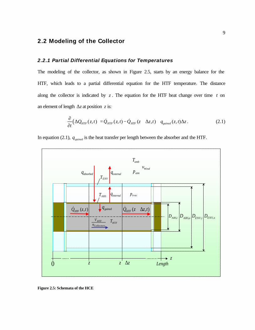
2.2.1 Partial Differential Equations for Temperatures The modeling of the collector, as shown in Figure 2.5, starts by an energy balance for the

HTF, which leads to a partial differential equation for the HTF temperature. The distance

along the collector is indicated by z . The equation for the HTF heat change over time t on

an element of length z∆ at position z is:

( )( , ) ( , ) ( , ) ( , )HTF HTF HTF gainedQ z t Q z t Q z z t q z t zt

∂∆ = − + ∆ + ∆

∂& & . (2.1)

In equation (2.1), gainedq is the heat transfer per length between the absorber and the HTF.

Figure 2.5: Schemata of the HCE

ENVT

ABST

HTFT

evacp

atmp

ambT

z z z+ ∆

iABSD , oABSD , iENVD , oENVD ,

z

absorbedq externalq

internalq

gainedq( , )HTFQ z t& ( , )HTFQ z z t+ ∆&

0 Length

Windv

Collectors

HTFn

V&

ENVT

ABST

HTFT

evacp

atmp

ambT

z z z+ ∆

iABSD , oABSD , iENVD , oENVD ,

z

absorbedq externalq

internalq

gainedq( , )HTFQ z t& ( , )HTFQ z z t+ ∆&

0 Length

Windv

Collectors

HTFn

V&

10From thermodynamics, it follows that

,( , ) ( , )HTF HTF HTF ABSi HTFQ z t c A zT z tρ∆ = ∆ (2.2)

with , ,HTF HTF HTFc Tρ as the HTF density, specific heat and temperature where the first two

depend on the latter. The cross-sectional area of the inside tube of the absorber is ,ABS iA . A

list with all the collector dimensions is given in Appendix A. It also follows from

thermodynamics

( , )( , )

( )( , )

HTFHTF

HTFHTF HTF HTF

Collectors

dQ z tQ z t

dtV t

c T z tn

ρ

=

=

&

& . (2.3)

Notice the overall HTF volume flow rate, HTFV& , depends only on the time t since the fluid is

considered to be incompressible. The number of collectors is Collectorsn . From Figure 2.1 it is

known that 50=Collectorsn . After inserting equation (2.2) and (2.3) into equation (2.1), it

follows that

,( , ) ( )

( , )

( )( , )

( , ) .

HTF HTFHTF HTF ABSi HTF HTF HTF

Collectors

HTFHTF HTF HTF

Collectors

gained

T z t V tc A z c T z t

t n

V tc T z z t

nq z t z

ρ ρ

ρ

∂∆ =

∂

− + ∆

+ ∆

&

& (2.4)

From the definition of the derivative it follows

0

( , ) ( , ) ( , )limHTF HTF HTF

z

T z t T z t T z z tz z∆ →

∂ − + ∆=

∂ ∆. (2.5)

11

Dividing equation (2.4) by z∆ , letting 0z∆ → and considering equation (2.5), yields the

following partial differential equation for the HTF temperature:

),(),()(),(

, tzqz

tzTn

tVc

ttzT

Ac gainedHTF

Collectors

HTFHTFHTF

HTFiABSHTFHTF +

∂∂

−=∂

∂ &ρρ . (2.6)

The boundary condition for equation (2.6) is

,(0, ) ( )HTF HTFinletT t T t= (2.7)

with ,HTFinletT as the HTF collector field inlet temperature. The initial condition for equation

(2.6) is

)()0,( , zTzT initHTFHTF = . (2.8)

In analogy to equation (2.1), the differential equation for the absorber temperature, ABST , is

obtained

( ) ( )( , ) ( ) ( , ) ( , )ABS absorbed internal gainedQ z t q t q z t q z t zt

∂∆ = − − ∆

∂. (2.9)

Here, internalq is the heat transfer per length between the absorber and the glass envelope. The

absorbed solar energy is absorbedq . From thermodynamics it is known that

( , ) ( , )ABS ABS ABS ABS ABSQ z t c A zT z tρ∆ = ∆ (2.10)

with , ,ABS ABS ABSc Tρ as the absorber density, specific heat and temperature. The cross-

sectional area of the absorber is ABSA . Substituting equation (2.10) into equation (2.9) yields

after a division by z∆

),(),()(),(

tzqtzqtqt

tzTAc gainedinternalabsorbed

ABSABSABSABS −−=

∂∂

ρ . (2.11)

12The initial condition for equation (2.11) is

)()0,( , zTzT initABSABS = . (2.12)

The glass envelope is assumed to have no radial temperature gradients. The differential

equation for the envelope temperature is gained through considerations similar to those used

to obtain the differential equation for the absorber temperature (2.11):

( , )( , ) ( , )ENV

ENV ENV ENV internal external

T z tc A q z t q z t

tρ

∂= −

∂ (2.13)

with , ,ENV ENV ENVc Tρ as the envelope density, specific heat and temperature. The heat

transfer per length between the envelope and the environment is externalq . The initial condition

for equation (2.13) is

)()0,( , zTzT initENVENV = . (2.14)

The interacting dynamic of the temperatures given through the differential equations (2.6),

(2.11) and (2.13) is determined by the heat transfer between the HTF, the absorber and the

envelope. It follows a discussion of equations to estimate the occurring heat transfer.

2.2.2 Heat Transfer between the Absorber and the HTF Considering convection for internal flow, the heat transfer, gainedq , is calculated through the

Dittus-Boelter equation for fully developed (hydrodynamically and thermally) turbulent flow

in a smooth circular tube (Incropera & De Witt, 2002). Hence, the local Nusselt number,

,A B S iDNu is given by

, ,

4 / 50.023A B S i A B S i

nD D HTFNu Re Pr= (2.15)

13

where n = 0.4 for heating ( ABS HTFT T> ) and 0.3 for cooling ( ABS HTFT T< ).

The Reynolds number, ,A B S iDRe , for flow in a circular tube, is given by

CollectorsHTFiABS

HTFHTFD nD

ViABS µπ

ρ

,

4Re

,

&= (2.16)

with HTFµ as the viscosity of the HTF. The Prandtl number, HTFPr , is determined by

HTFHTF

HTF

Prνα

= (2.17)

with the kinematic viscosity of the HTF, HTFν , defined by

HTFHTF

HTF

µν

ρ= (2.18)

and the thermal diffusivity of the HTF, HTFα , which is given through

HTFHTF

HTFHTF c

kρ

α = . (2.19)

Within equation (2.19), HTFk is the thermal conductivity of the HTF. The heat transfer

coefficient, ,ABSHTFh , is calculated by using the local Nusselt number, ,A B S iDNu , through

,

,,

A B S iD HTFABSHTF

ABS i

Nu kh

D= , (2.20)

where ,A B S iD is the inside diameter of the absorber tube and 066.0, =iABSD m. The HTF

properties HTFc , HTFk , HTFµ and HTFρ are functions of the HTF temperature, HTFT . Finally

the heat transfer between the absorber and the HTF, gainedq , is calculated as

( ), , ,gained ABS HTF ABSsur f i ABS HTFq h A T T= − (2.21)

14

with the inner surface area per length of the absorber, , ,ABS surf iA ,

, , ,ABS surf i ABS iA Dπ= . (2.22)

2.2.3 Heat Transfer between the Absorber and the Glass Envelope The heat transfer between the absorber and the glass envelope, internalq , is calculated from

convection and radiation

, ,internal internalconvection internalradiat ionq q q= + . (2.23)

Assuming only partial evacuation of the annulus between the absorber and the glass

envelope, the occurring free convection is estimated through relations for a free convection

flow in the annular space between long, horizontal, concentric cylinders (Incropera & De

Witt, 2002). Since the glass envelope is usually cooler than the absorber ( ABS ENVT T> ), the air

ascends along the absorber and descends along the glass envelope. The convection heat

transfer, ,internalconvectionq , may be expressed as

eff,,

, ,

2( )

ln( / )Air

internalconvection ABS ENVENV i A B S o

kq T T

D Dπ

= − (2.24)

where ,ENV iD is the inside diameter of the glass envelope ( 112.0, =iENVD m) and ,A B S oD is

the outside diameter of the absorber ( 07.0, =oABSD m). The effective thermal conductivity,

eff ,Airk , is the thermal conductivity that the stationary air should have to transfer the same

amount of heat as moving air. A suggested correlation for eff ,Airk is

1 /4

eff , * 1 /40.386 ( )0.861

Air Airc

Air Air

k PrRa

k Pr

= + (2.25)

15where

4

, ,*3 3/5 3/5 5

, ,

ln( / )

( )ENV i ABS o

c LABS o ENV i

D DRa Ra

L D D− −

=+

. (2.26)

In equation (2.25), AirPr , is the Prandtl number of air in the annulus. The thermal

conductivity of air is Airk . In equation (2.26), L , is the effective length and is given for the

annulus through

( ), ,0.5 E N V i A B S oL D D= − . (2.27)

The Rayleigh Number of air, LRa , is defined as

( )AirAir

ENVABSAirL

LTTgRa

ναβ 3−

= (2.28)

withg as the gravitational acceleration ( -2sm81.9=g ), the volumetric thermal expansion

coefficient of air, Airβ , and the thermal diffusivity of air, Airα , calculated as

AirpAir

AirAir c

k

,ρα = . (2.29)

Here, Airρ is the density of air in the annulus and Airpc , is the specific heat of air. The

kinematic viscosity of air, Airν , is given by

Air

AirAir ρ

µν = (2.30)

with the viscosity of air, Airµ . The properties of air in the annulus, Airα , Airβ , Airpc , , Airk ,

Airµ , Airν , AirPr and Airρ are dependent on the mean temperature in the annulus

( )ENVABSAnnulus TTT += 5.0 . (2.31)

16

In addition, the density Airρ depends on the evacuation pressure in the annulus, evacp . A

value of 7=evacp kPa is used in the model. This value was chosen such that the calculated

collector outlet temperature fits the measured collector outlet temperature best.

The heat transfer through radiation between long, concentric cylinders, ,internalradiationq ,

may be expressed as (Incropera & De Witt, 2002)

( )4 4, ,

,,

,

11ABSsur f o ABS ENV

internalradiationABS oENV

ABS ENV ENV i

A T Tq

DD

σ

εε ε

−=

−+

. (2.32)

In equation (2.32), σ is the Stefan-Boltzmann constant and has the numerical value

428 KW/m10670.5 ⋅×= −σ .

The outer surface area per length of the absorber, , ,ABS surf oA , is given by

, , ,ABS surf o ABS oA Dπ= . (2.33)

The emissivity of the absorber is ABSε and the emissivity of the glass envelope is ENVε with

9.0=ENVε as measured by SANDIA. The emissivity of the absorber, ABSε , increases with the

absorber temperature, ABST . SANDIA provides a linear function for ABSε from their

measurements:

065971.0000327.0 −⋅= ABSABS Tε . (2.34)

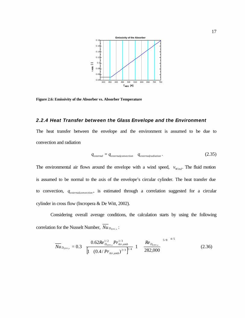
If ABSε < 0.05 then the value is set to ABSε = 0.05 (Figure 2.6).

17

300 350 400 450 500 550 600 650 700 7500.04

0.06

0.08

0.1

0.12

0.14

0.16

0.18

TABS [K]

ε ABS

[-]

Emissivity of the Absorber

Figure 2.6: Emissivity of the Absorber vs. Absorber Temperature 2.2.4 Heat Transfer between the Glass Envelope and the Environment The heat transfer between the envelope and the environment is assumed to be due to

convection and radiation

, ,external externalconvection externalradiationq q q= + . (2.35)

The environmental air flows around the envelope with a wind speed, Windv . The fluid motion

is assumed to be normal to the axis of the envelope’s circular cylinder. The heat transfer due

to convection, ,externalconvectionq , is estimated through a correlation suggested for a circular

cylinder in cross flow (Incropera & De Witt, 2002).

Considering overall average conditions, the calculation starts by using the following

correlation for the Nusselt Number, oENVDNu , :

[ ]

5/48/5

4/13/2,

3/1,

2/1

000,2821

)/4.0(1

62.03.0 ,,

,

+

++= oENVoENV

oENV

D

ambAir

ambAirDD

Re

Pr

PrReNu (2.36)

18

For the circular glass envelope cylinder, the Reynolds Number, oENVDRe

,, is defined as

ambAir

oENVWindambAirD

DvRe

oENV,

,,, µ

ρ= (2.37)

with ambAir,ρ as the density of the ambient air, oENVD , as the outside diameter of the glass

envelope ( 115.0, =oENVD m) and ambAir,µ as the viscosity of the ambient air. The Prandtl

number of the ambient air is ambAirPr , . The convection heat transfer coefficient, tEnvironmenENVh , ,

is then given through

oENV

ambAirDtEnvironmenENV

DkNu

h oENV

,

,,

,= . (2.38)

The thermal conductivity of the ambient air, ambAirk , , and the other properties of the air,

ambAir,µ , ambAirPr , and ambAir,ρ are dependent on the mean ambient temperature

( )ambENVamb TTT += 5.0 , (2.39)

where ambT is the ambient temperature of the environment. In addition, ambAir,ρ depends on the

atmospheric pressure, atmp . Finally, the heat transfer to the environment due to convection is

( ),, , ,ENVEnvironmentexternalconvection ENVsur f o ENV ambq h A T T= − (2.40)

with the outer surface area per length of the glass envelope, , ,ENV s u r f oA , calculated through

, , ,ENV surf o ENV oA Dπ= . (2.41)

The heat transfer to the environment due to radiation, radiationexternalq , , may be expressed as

(Incropera & De Witt, 2002)

( )4 4, , ,externalradiation ENV ENV surf o ENV ambq A T Tε σ= − (2.42)

19

with ENVε as the emissivity of the glass envelope. This relationship describes the radiation of

a small convex object, the glass envelope, in a large cavity, the environment.

The sun’s energy is the energy source that acts on the absorber and induces the heat

transfer discussed above. It governs the amount of energy finally transferred to the HTF and

thus to the power plant for the generation of electricity. Thus, it is necessary to estimate the

amount of absorbed solar energy, absorbedq .

2.2.5 Absorbed Solar Energy The following discussion is based on (Duffie & Beckman, 1991) and (Iqbal, 1983). The sun

is a completely gaseous body. Gravitational forces retain its constituent hot gases. The sun’s

physical structure is complex and may be considered to be composed of several regions,

where the innermost region, the core, is the hottest and densest part. Above the core is the

interior, which contains practically all of the sun’s mass. The core and the interior are

considered as a continuous fusion reactor, the source of almost all the sun’s energy. This

energy is propagated to the outer regions. The sun’s surface, the photosphere, is the source of

most solar radiation arriving at the earth’s atmosphere.

The intensity of solar radiation outside of the earth’s atmosphere is nearly fixed about

1.37 kW/m2 for the mean distance between the earth and the sun of one astronomical unit, 1

AU = 1110496.1 × m. It varies with the earth-sun distance over the year in the range of %3± .

The earth is at its closest point to the sun (perihelion; ≈ 0.983 AU) on approximately 3

January and at its farthest point (aphelion; ≈ 1.017 AU) on approximately 4 July. The mean

distance is approached at approximately 4 April and 5 October. The amount of solar radiation

20reaching the earth’s atmosphere is inversely proportional to the square of its distance from

the sun.

When solar radiation enters the earth’s atmosphere, a part of the incident energy is

removed by scattering in the atmosphere due to interaction of the radiation with air

molecules, water (vapor and droplets), and dust. Another part of the incident energy is

removed in the earth’s atmosphere by absorption of radiation in the solar energy spectrum

due to ozone in the ultraviolet and to water vapor and carbon dioxide in bands in the infrared.

The scattered radiation is called diffuse radiation. A portion of this diffuse radiation goes

back to space and a portion reaches the ground. The remaining part of the solar radiation that

enters the earth’s atmosphere, the radiation arriving on the ground directly in line from the

solar disk without having been scattered by the atmosphere or having been absorbed, is

called beam radiation. Beam radiation incident on a plane normal to the radiation is called the

direct normal radiation. The total solar radiation or global radiation, that is, the sum of the

diffuse and beam solar radiation on a surface, is important for the design of flat-plate

collectors or for the calculations of heating and cooling loads in architecture. For

concentrating systems like the solar trough collector field only the beam radiation or direct

normal radiation is used.

The direct normal radiation, bnG , can be measured by using a Normal Incidence

Pyrheliometer (NIP). The NIP is an instrument for measuring solar radiation from the sun

and from a small portion of the sky around the sun at normal incidence.

21

Figure 2.7: Direct normal radiation vs. time for June 20, 1998 (left hand figure) and for December 16, 1998 (right hand figure)

Figure 2.7 shows the direct normal radiation vs. time for a day measured with a NIP at SEGS

VI. The left hand figure shows the measurement for a clear (no clouds) spring/summer day,

June 20, 1998 and the right hand figure shows the beam radiation during a clear fall/winter

day, December 16, 1998.

Notice the direct normal radiation is not constant between sunrise and sunset because

the effects of the atmosphere in scattering and absorbing radiation are variable with time as

atmospheric conditions and air mass change.

In order to maximize the energy from the solar beam radiation through the

concentrating trough collectors, the surface normal of a collector has to be collinear to the

vector of the incoming solar beam radiation. The angle of incidence, θ , is the angle between

the beam radiation on a surface and the normal to that surface. Throughout the sun’s daily

path between sunrise and sunset, the sun changes its solar position in the sky. Consequently,

during a day, the vector of the incoming solar beam radiation changes its direction as well.

To minimize the angle of incidence, the solar collectors must track the sun by moving in

5 6 7 8 9 10 11 12 13 14 15 16 17 18 19 20 21 220

200

400

600

800

1000

Time [hr]

Gb

n [

W/m

^2]

Direct Normal Radiation, June 20, 1998

5 6 7 8 9 10 11 12 13 14 15 16 17 18 19 20 21 220

200

400

600

800

1000

Time [hr]

Gb

n [

W/m

^2]

Direct Normal Radiation, December 16, 1998

22prescribed ways. The best way to track the sun is by rotating the collector’s surface about

two axis. As can be seen in Figure 2.1, the solar collector troughs of SEGS VI are tracking

the sun by rotating around a single axis, which is the horizontal north-south axis. Due to this

constraint movability, only the component of the solar beam radiation vector, which is

collinear to the normal of the single-axis-tracking collector surface, remains to heat the

absorber, as shown in Figure 2.8. This component of the solar beam radiation vector may be

found by multiplying the amount of solar beam radiation with the cosine of the angle of

incidence. Therefore a relationship for the angle of incidence is needed, which is given by

(Duffie & Beckman, 1991)

( ) 2/1222 sincoscoscos ωδθθ += z . (2.43)

On the right hand side of this equation, there are three angles, δθ ,z and ω , which describe

the position of the sun for its daily path and will be explained in the following (Figure 2.9,

(Iqbal, 1983)).

Figure 2.8: North-South Tracking

South

East

Surface Normal

Beam Radiation

Angle of Incidence

..

South

East

Surface Normal

Beam Radiation

Angle of Incidence

..

23In Figure 2.9, a celestial sphere is drawn with the earth as the center. In the celestial sphere,

the celestial poles are the points at which the earth’s extended polar axis cuts the celestial

sphere. Similarly, the celestial equator is an outward projection of the earth’s equatorial plane

on the celestial sphere. At any given time, the collector on the earth’s surface has a

corresponding position in the celestial sphere called the collector’s zenith: this is the point of

intersection with the celestial sphere of a normal to the earth’s surface at the collector’s

position. The collector’s horizon is a great circle in the celestial sphere described by a plane,

which passes through the center of the earth normal to the line joining the center of the earth

and the zenith.

Figure 2.9: Celestial sphere and sun’s coordinates relative to collector on earth at point C

zθ

δω

Earth

Sun

Local Zenith

Noon

Collector’sSouth

C

Collector’sNorth

Local Nadir

Collector’s

Celestial Horizon

Celestial Equator

CelestialNorth Pole

CelestialSouth Pole

Earth’s Celestia

l Axis

East

φ

zθ

δω

Earth

Sun

Local Zenith

Noon

Collector’sSouth

C

Collector’sNorth

Local Nadir

Collector’s

Celestial Horizon

Celestial Equator

CelestialNorth Pole

CelestialSouth Pole

Earth’s Celestia

l Axis

East

φ

24

The zenith angle, zθ , is the angle between the vertical (the local zenith) and the line to the

sun, that is the angle of incidence of beam radiation, θ , on a horizontal surface. The angle is

within a range of °≤≤° 900 zθ . Since the trough collectors are tracking surfaces, they are

horizontal only at solar noon and thus the zenith angle is equal to the angle of incidence of

beam radiation only at solar noon.

The declination, δ , is the angular position of the sun at solar noon (i.e., when the sun

is on the local meridian) with respect to the plane of the equator, north positive; the

declination angle is within a range of °≤≤°− 45.2345.23 δ . It reaches its minimum value at

the winter solstice (21/22 December) and its maximum value at the summer solstice (21/22

June). The angle is zero at the vernal equinox (20/21 March) and at the autumnal equinox

(22/23 September). In 24 h, the maximum change in declination (which occurs at the

equinoxes) is less than °21 . See also Figure 2.10 where the solar declination is described by

drawing a celestial sphere with the earth at the center and the sun revolving around the earth

in a year. Several expressions giving the approximate value of solar declination have been

suggested.

Spencer presented the following expression for δ , in degrees (Spencer, as quoted by

Iqbal, 1983):

)./180))(3sin(00148.0)3cos(002697.0)2sin(000907.0)2cos(006758.0

sin070257.0cos399912.0006918.0(

π

δ

Γ+Γ−Γ+Γ−

Γ+Γ−= (2.44)

In this equation, Γ , in radiants, is called the day angle. It is represented by

( ) 365/12 −=Γ ndπ , (2.45)

25

where nd is the day number of the year, ranging from 1 on 1 January to 365 on 31 December.

February is always assumed to have 28 days. Equation (44) estimates δ with a maximum

error of 0.0006 rad (<3’) and is recommended for use in digital machines.

Another equation obtained by Perrin de Brichambaut is, in degrees (Brichambaut, as quoted

by Iqbal, 1983),

( )[ ]{ }82sin4.0sin 3653601 −= −

ndδ . (2.46)

Figure 2.10: Celestial Sphere showing sun’s declination angle

SummerSolstice

WinterSolstice

Sun

Earth

N

S

AutumnalEquinox

VernalEquinox

δ

North Pole ofCelestial Sphere

South Pole ofCelestial Sphere

Apparent Path of Sun onThe Ecliptic Plane

Plane of CelestialEquator

90°

≈ 23.5°

≈ 23.5°

SummerSolstice

WinterSolstice

Sun

Earth

N

S

AutumnalEquinox

VernalEquinox

δ

North Pole ofCelestial Sphere

South Pole ofCelestial Sphere

Apparent Path of Sun onThe Ecliptic Plane

Plane of CelestialEquator

90°

≈ 23.5°

≈ 23.5°

26A further and simple equation found by Cooper is, in degrees (Cooper, as quoted by Iqbal

1983),

( )[ ].284sin45.23 365360 += ndδ (2.47)

A plot of the declination,δ , vs. month is shown in Figure 2.11.

The hour angle, ω , is the angular displacement of the sun east or west of the local

meridian due to rotation of the earth on its axis at 15° per hour, morning negative, afternoon

positive. The hour angle, ω , is 0° at solar noon.

Figure 2.11: Declination vs. Month

The solar noon (i.e., the sun is on the local meridian) does not coincide with the local clock

noon (Duffie & Beckman, 1991). It is necessary to convert standard time to solar time by

applying two corrections. First, there is a constant correction for the difference in longitude

between the observer’s meridian (longitude) and the meridian on which the local standard

time is based. The SEGS VI plant is located at the local longitude, locL , of 117.022°W. The

-25

-20

-15

-10

-5

0

5

10

15

20

25

Month

δ [

deg

]

J F M A M J J A S O N D

Declination

27

local clock time is measured with respect to the standard longitude, stL , of 120°W for the

Pacific Standard Time. The sun takes 4 minutes to transverse 1° of longitude. A second

correction is from the equation of time, which takes into account the perturbations in the

earth’s rate of rotation, which affects the time the sun crosses the collector’s meridian. Thus,

in minutes,

( ) tlocst ELL +−⋅= 4 Time Standard-TimeSolar (2.48)

where tE is the equation of time, again from Spencer (Spencer, as quoted by Iqbal, 1983):

())2sin(04089.0)2cos(014615.0

sin032077.0cos001868.0007500.018.229Γ−Γ−

Γ−Γ+=tE . (2.49)

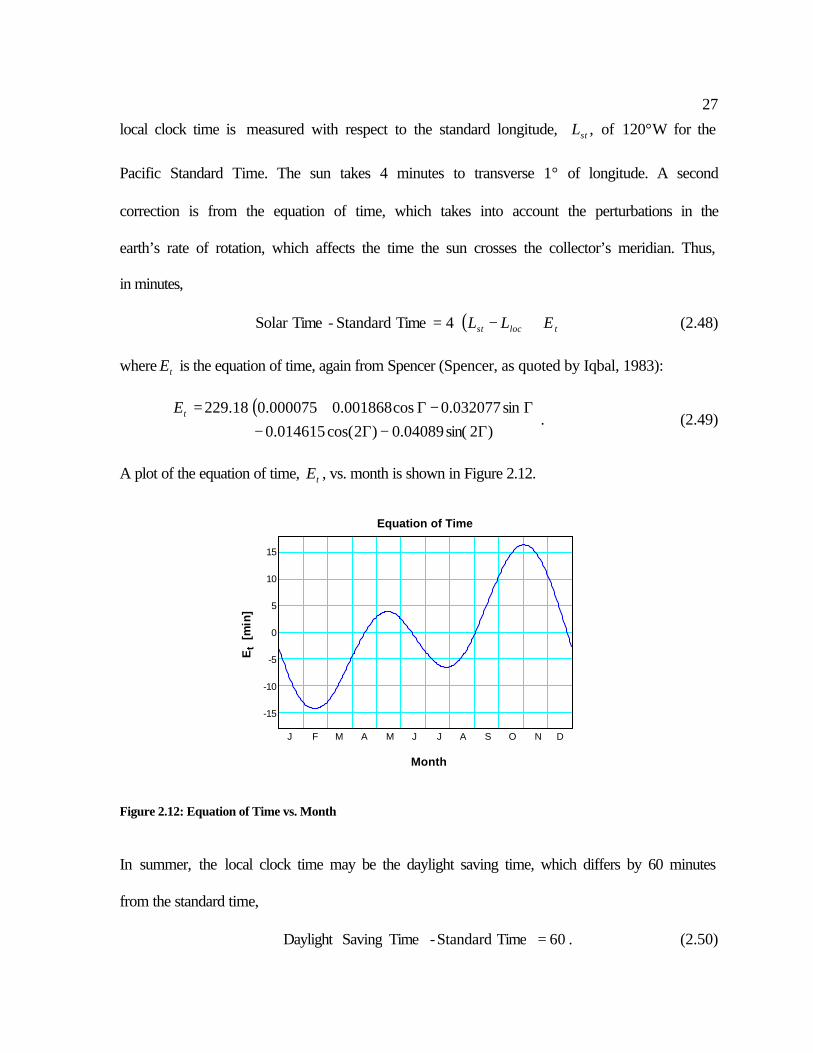
A plot of the equation of time, tE , vs. month is shown in Figure 2.12.

Figure 2.12: Equation of Time vs. Month

In summer, the local clock time may be the daylight saving time, which differs by 60 minutes

from the standard time,

60 Time Standard - Time SavingDaylight = . (2.50)

-15

-10

-5

0

5

10

15

Month

Et

[min

]

J F M A M J J A S O N D

Equation of Time

28

A fourth angle in Figure 2.9 is the latitude, φ , and gives the position of the collector north or

south from the earth’s equator. The SEGS VI plant is located at N35°=φ .

There is a useful relationship among the four angles given in Figure 2.9. An equation relating

the zenith angle, zθ , to the others is (Duffie & Beckman, 1991)

δφωδφθ sinsincoscoscoscos +=z . (2.51)

This equation can be used to solve for the value of the hour angle, ω , at sunset. At sunset,

the zenith angle, zθ , is 90° when the sun is at the horizon. Thus, the sunset hour angle,

sunsetω , in degrees, is given by

δφω tantancos −=sunset . (2.52)

The sunrise hour angel, sunriseω , is consequently

sunsetsunrise ωω −= . (2.53)

Assuming that the time for the solar noon calculated from equation (2.48) is converted from

minutes into hours, the following equation gives the time at sunrise in hours from the fact

that the sun rotates with 15° per hour:

15/ Noon Solar Hour Sunrise sunriseω+= . (2.54)

Finally, an expression for the hour angle, ω , is given through

15Hour) Sunrise - Time(Solar ⋅+= sunriseωω . (2.55)

Here, the solar time is calculated from equation (2.48) after converting the result from

minutes into hours.

The zenith angle, zθ , given by equation (2.51), the declination, δ , given by equation

(2.44) and the hour angle, ω , equation (2.55), are inserted into equation (2.43) to calculate

29the angle of incidence. Thus, multiplying the cosine of the angle of incidence with the

magnitude of solar beam radiation gives the reduced beam radiation acting on an unshaded

single-axis-tracking collector.

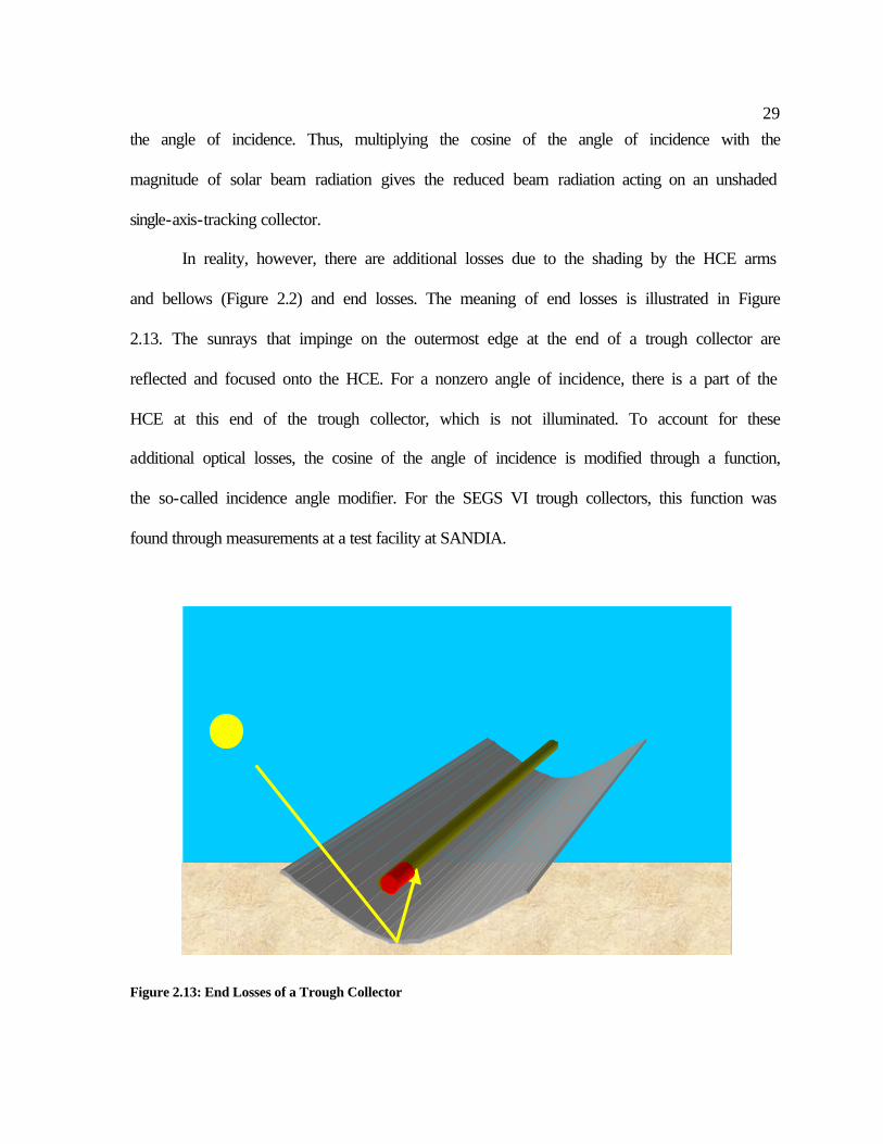
In reality, however, there are additional losses due to the shading by the HCE arms

and bellows (Figure 2.2) and end losses. The meaning of end losses is illustrated in Figure

2.13. The sunrays that impinge on the outermost edge at the end of a trough collector are

reflected and focused onto the HCE. For a nonzero angle of incidence, there is a part of the

HCE at this end of the trough collector, which is not illuminated. To account for these

additional optical losses, the cosine of the angle of incidence is modified through a function,

the so-called incidence angle modifier. For the SEGS VI trough collectors, this function was

found through measurements at a test facility at SANDIA.

Figure 2.13: End Losses of a Trough Collector

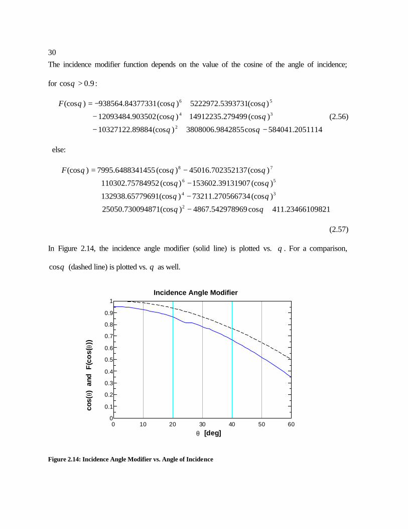
30The incidence modifier function depends on the value of the cosine of the angle of incidence;

for 9.0cos >θ :

2051114.584041cos9842855.3808006)(cos89884.10327122

)(cos279499.14912235)(cos903502.12093484

)(cos5393731.5222972)(cos84377331.938564)(cos

2

34

56

−+−

+−

+−=

θθ

θθ

θθθF

(2.56)

else:

12346610982.411cos542978969.4867)(cos730094871.25050

)(cos270566734.73211)(cos65779691.132938

)(cos39131907.153602)(cos75784952.110302

)(cos702352137.45016)(cos6488341455.7995)(cos

2

34

56

78

+−+

−+

−+

−=

θθ

θθ

θθ

θθθF

(2.57)

In Figure 2.14, the incidence angle modifier (solid line) is plotted vs. θ . For a comparison,

θcos (dashed line) is plotted vs. θ as well.

Figure 2.14: Incidence Angle Modifier vs. Angle of Incidence

0 10 20 30 40 50 600

0.1

0.2

0.3

0.4

0.5

0.6

0.7

0.8

0.9

1

θ [deg]

cos(

θ) a

nd F

(co

s(θ)

)

Incidence Angle Modifier

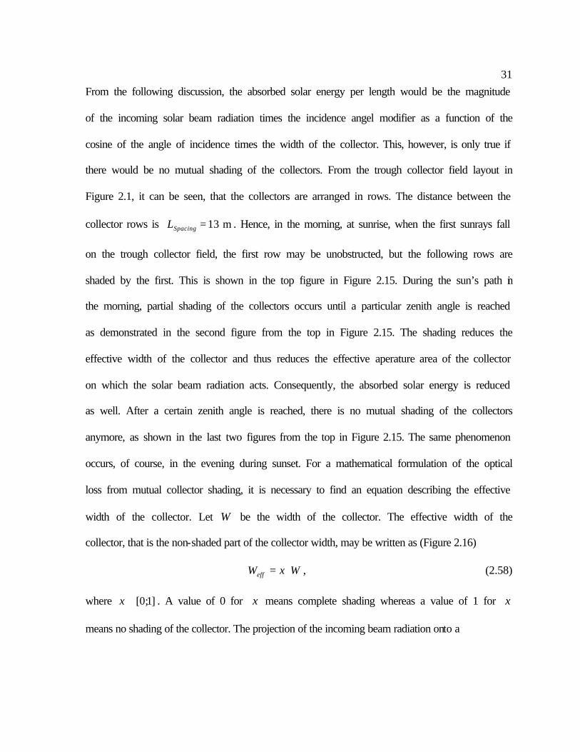
31From the following discussion, the absorbed solar energy per length would be the magnitude

of the incoming solar beam radiation times the incidence angel modifier as a function of the

cosine of the angle of incidence times the width of the collector. This, however, is only true if

there would be no mutual shading of the collectors. From the trough collector field layout in

Figure 2.1, it can be seen, that the collectors are arranged in rows. The distance between the

collector rows is m13=SpacingL . Hence, in the morning, at sunrise, when the first sunrays fall

on the trough collector field, the first row may be unobstructed, but the following rows are

shaded by the first. This is shown in the top figure in Figure 2.15. During the sun’s path in

the morning, partial shading of the collectors occurs until a particular zenith angle is reached

as demonstrated in the second figure from the top in Figure 2.15. The shading reduces the

effective width of the collector and thus reduces the effective aperature area of the collector

on which the solar beam radiation acts. Consequently, the absorbed solar energy is reduced

as well. After a certain zenith angle is reached, there is no mutual shading of the collectors

anymore, as shown in the last two figures from the top in Figure 2.15. The same phenomenon

occurs, of course, in the evening during sunset. For a mathematical formulation of the optical

loss from mutual collector shading, it is necessary to find an equation describing the effective

width of the collector. Let W be the width of the collector. The effective width of the

collector, that is the non-shaded part of the collector width, may be written as (Figure 2.16)

WxWeff ⋅= , (2.58)

where ]1;0[∈x . A value of 0 for x means complete shading whereas a value of 1 for x

means no shading of the collector. The projection of the incoming beam radiation onto a

32

Figure 2.15: Illustration of mutual shading in a multirow collector array

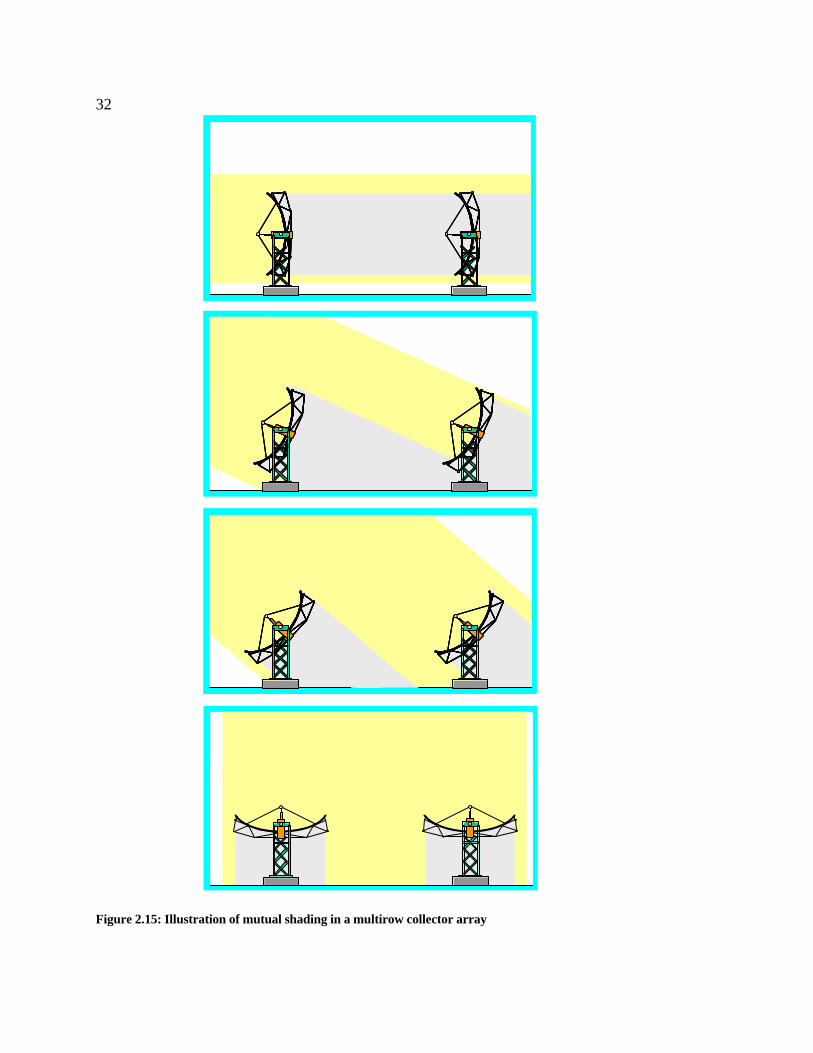
33plane perpendicular to the collector’s rotational north-south axis yields a radiation, which

direction is given by the profile angle pα (Figure 2.16 and Figure 2.17).

Figure 2.16: Mutual Collector Shading

Trigonometric considerations (Figure 2.16) yield

Wx

WxW

L PSpacing

⋅=

−−=

21

2)sin( α

(2.59)

The law of cosines for the spherical triangle O, Sun, P, Z in Figure 2.17 results in

)sin()cos(

)90cos()90sin()sin()90cos()cos()cos(

p

ppz

αθ

αθαθθ

=

°−°+−°=. (2.60)

pα

SpacingL

2W

2W

(1 )x W−

x W⋅

( )12 x W−

1st Collector2nd Collector

Shading

Limiting Sunray

pα

SpacingL

2W

2W

(1 )x W−

x W⋅

( )12 x W−

1st Collector2nd Collector

Shading

Limiting Sunray

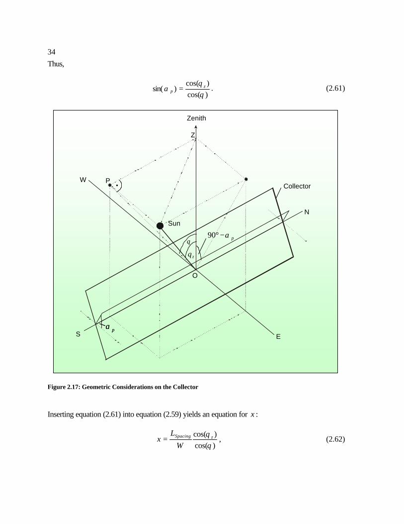
34Thus,

)cos()cos(

)sin(θθ

α zp = . (2.61)

Figure 2.17: Geometric Considerations on the Collector

Inserting equation (2.61) into equation (2.59) yields an equation for x :

)cos()cos(

θθ zSpacing

W

Lx = , (2.62)

pα

zθ

90 pα° −θ

N

S E

W

Zenith

Collector

Sun

O

P

Z

pα pα

zθ

90 pα° −θ

N

S E

W

Zenith

Collector

Sun

O

P

Z

35

where it is necessary to restrict x to be in the interval between 0 and 1:

= 0.1;

)cos()cos(

;0.0maxminθθ zSpacing

W

Lx . (2.63)

The equation for the effective width, effW , is finally given through inserting equation (2.63)

into equation (2.58),

WW

LW zSpacing

eff ⋅

= 0.1;

)cos()cos(

;0.0maxminθθ

. (2.64)

After discussing the optical energy losses due to the tracking geometry and shading,

additional optical energy losses due to radiation characteristics of the mirror, the envelope

and the absorber have to be accounted.

First, the incident solar beam radiation is reflected on the trough mirror and directed

onto the HCE. Two cases of reflection occur, specular reflection and diffuse reflection

(Duffie & Beckman, 1991). The diffuse reflection distributes the radiation in all directions

and thus the part of the incident solar beam radiation that is reflected through diffuse

reflection on the trough mirrors does not contribute noticeably to the beam radiation acting

on the absorber. The specular reflected part of the incident solar beam radiation is the

remaining source for absorbed solar energy. The specular reflectance, ρ , is defined as the

fraction of the specular reflected beam radiation to the incident solar beam radiation on the

trough mirror. Measurements of the specular reflectance, ρ , accomplished at a test facility at

SANDIA, yield a value of 94.0=ρ .

The remaining specular reflected solar beam radiation is transmitted through the glass

envelope of the HCE before it is absorbed. When radiation passes from one medium with a

36particular refractive index to a second medium with a different refractive index, there is

reflection occurring at the interface between the two media (Duffie & Beckman, 1991). A

part of the incoming radiation is reflected while the remaining part enters the second

medium. The glass envelope of the HCE is a cover with two interfaces to cause reflection

losses. A part of the incoming solar beam radiation is reflected at the first interface as

discussed before. The remaining part is passed through the glass where it reaches the second

interface. Of the remaining part, a portion passes through the second interface and the other

portion is reflected back to the first interface, and so on. Summing up the parts of the solar

beam radiation that passed through the second interface yields the amount of radiation that

may be absorbed by the absorber when absorption of the glass envelope is neglected. If it is

not neglected, then there is an additional absorption loss through the glass material and the

remaining solar beam radiation acting on the absorber is even further reduced. The definition

of the transmittance,τ , accounts for the radiation losses through reflection and absorption of

the glass envelope. The transmittance, τ , is the fraction of the remaining solar beam

radiation after transmission through the glass envelope to the incoming specular reflected

solar beam radiation. The transmittance, τ , was measured to 915.0=τ .

Finally, the reflected and transmitted solar beam radiation is absorbed by the surface

of the absorber tube in the HCE. The absorptance, α , is defined as the fraction of the solar

beam radiation absorbed by the surface over the incoming reflected and transmitted solar

beam radiation. SANDIA measured the absorptance, α , to be 94.0=α .

In the annulus between the absorber tube and the glass envelope, the radiation, which

is not absorbed by the absorber but instead reflected back to the glass envelope, is partially

reflected at the glass envelope back to the absorber again where part of it may now be

37absorbed. That’s why there is a slight increase of the absorbed solar beam radiation

compared to the radiation from single absorption, accounted through the definition of the

transmittance-absorptance product )(τα (Duffie & Beckman, 1991). For most practical solar

collectors, a reasonable approximation is

τατα 01.1)( ≅ . (2.65)

Combining the results from above, the optical efficiency from radiation characteristics is

)(ταρε =opt . (2.66)

Finally, an expression for the absorbed solar energy is found:

γεθ opteffbnabsorbed WFGq )(cos= . (2.67)

In equation (2.67), γ is a factor varying from one day to the other. Different amount of dirt

on the mirrors and the number of broken collectors in the field influence this factor.

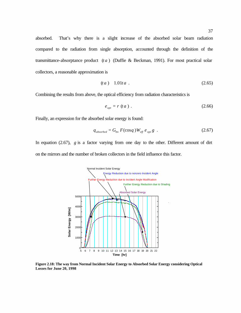
Figure 2.18: The way from Normal Incident Solar Energy to Absorbed Solar Energy considering Optical Losses for June 20, 1998

5 6 7 8 9 10 11 12 13 14 15 16 17 18 19 20 21 220

1000

2000

3000

4000

5000

Time [hr]

So

lar

En

erg

y [

W/m

]

Normal Incident Solar Energy

Energy Reduction due to nonzero Incident Angle

Further Energy Reduction due to Incident Angle Modification

Further Energy Reduction due to Shading

Absorbed Solar Energy

38

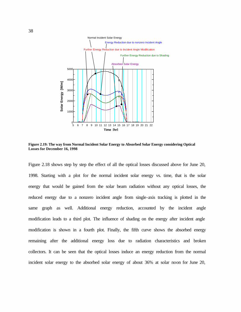
Figure 2.19: The way from Normal Incident Solar Energy to Absorbed Solar Energy considering Optical Losses for December 16, 1998

Figure 2.18 shows step by step the effect of all the optical losses discussed above for June 20,

1998. Starting with a plot for the normal incident solar energy vs. time, that is the solar

energy that would be gained from the solar beam radiation without any optical losses, the

reduced energy due to a nonzero incident angle from single-axis tracking is plotted in the

same graph as well. Additional energy reduction, accounted by the incident angle

modification leads to a third plot. The influence of shading on the energy after incident angle

modification is shown in a fourth plot. Finally, the fifth curve shows the absorbed energy

remaining after the additional energy loss due to radiation characteristics and broken

collectors. It can be seen that the optical losses induce an energy reduction from the normal

incident solar energy to the absorbed solar energy of about 36% at solar noon for June 20,

5 6 7 8 9 10 11 12 13 14 15 16 17 18 19 20 21 220

1000

2000

3000

4000

5000

Time [hr]

So

lar

En

erg

y [

W/m

]

Normal Incident Solar Energy

Energy Reduction due to nonzero Incident Angle

Further Energy Reduction due to Incident Angle Modification

Further Energy Reduction due to Shading

Absorbed Solar Energy

391998. The result is worse for December 16, 1998, shown in Figure 2.19, where the reduction

is about 76% at solar noon.

2.3 Model Implementation and Simulation Results The equations and expressions discussed above form a physical model for the trough

collector field. This model can be used to predict the outlet temperature vs. time of the

collector field when the inlet temperature of the collector field, the volume flow rate of the

HTF and environmental data vs. time are known. The environmental data consist of normal

incident solar radiation, ambient temperature and wind speed. Figure 2.20 shows the

collector model as a block with inputs and the output. An accurate calculation of the collector

field outlet temperature is necessary because the objective of the control problem is to hold

this particular temperature at a constant value. Solutions of the partial differential equations

(PDEs), (2.6), (2.11) and (2.13), have to be found in order to calculate the collector field

outlet temperature. Analytical solutions are not possible due to the nonlinearity and

complexity of the PDEs. Therefore, numerical integration was chosen for the calculation

strategy. Hence, the equations from above have to be prepared for an implementation in

digital machines.

Figure 2.20: The Collector Model as a Block with Inputs and Output

CollectorModel

Inlet Temperature

VolumeFlow Rate

SolarRadiation

AmbientTemperature

WindSpeed

OutletTemperatureCollector

Model

Inlet TemperatureInlet Temperature

VolumeFlow RateVolumeFlow Rate

SolarRadiationSolarRadiation

AmbientTemperatureAmbientTemperature

WindSpeedWindSpeed

OutletTemperatureOutletTemperature

40

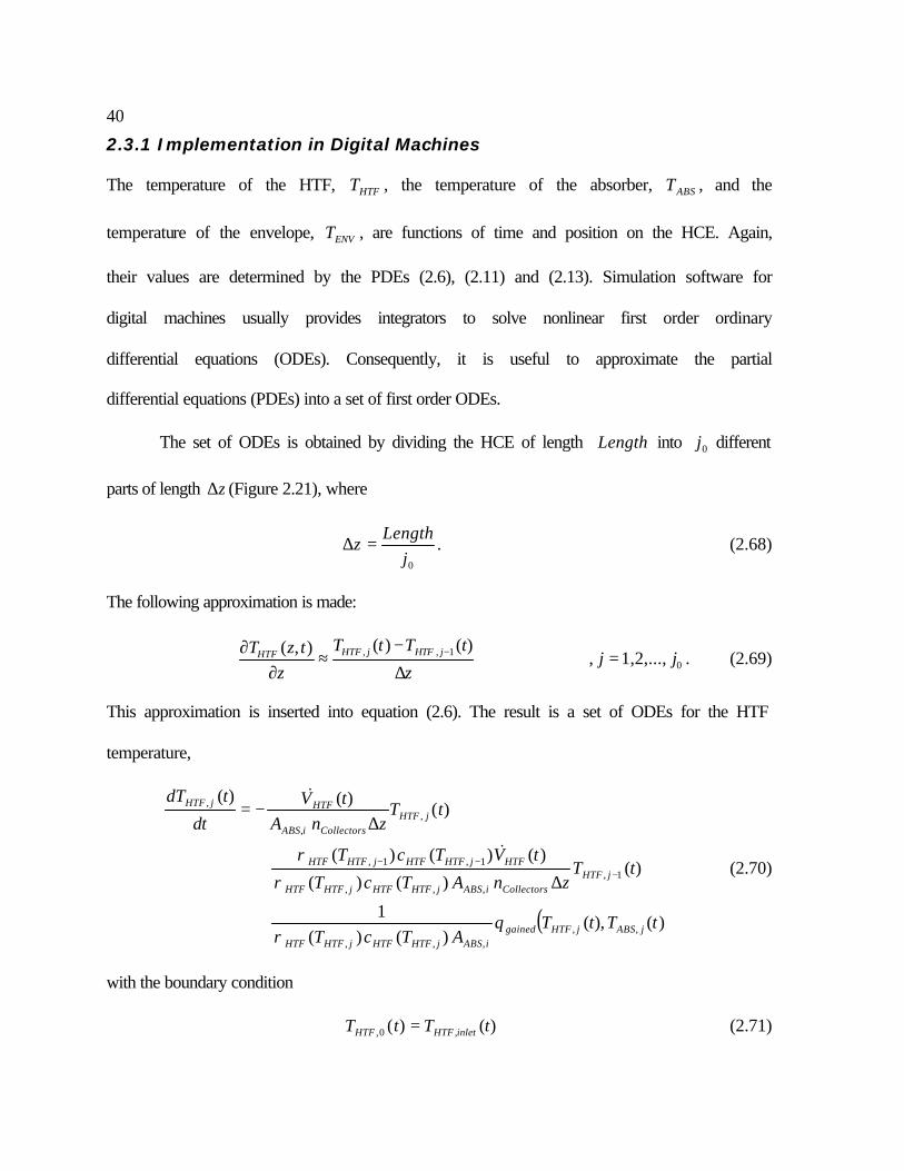
2.3.1 Implementation in Digital Machines The temperature of the HTF, HTFT , the temperature of the absorber, ABST , and the

temperature of the envelope, ENVT , are functions of time and position on the HCE. Again,

their values are determined by the PDEs (2.6), (2.11) and (2.13). Simulation software for

digital machines usually provides integrators to solve nonlinear first order ordinary

differential equations (ODEs). Consequently, it is useful to approximate the partial

differential equations (PDEs) into a set of first order ODEs.

The set of ODEs is obtained by dividing the HCE of length Length into 0j different

parts of length z∆ (Figure 2.21), where

0jLength

z =∆ . (2.68)

The following approximation is made:

, , 10

( ) ( )( , ), 1,2,...,HTF j HTF jHTF

T t T tT z tj j

z z−−∂

≈ =∂ ∆

. (2.69)

This approximation is inserted into equation (2.6). The result is a set of ODEs for the HTF

temperature,

( ))(),()()(

1

)()()(

)()()(

)()()(

,,,,,

1,,,,

1,1,

,,

,

tTtTqATcT

tTznATcT

tVTcT

tTznA

tVdt

tdT

jABSjHTFgainediABSjHTFHTFjHTFHTF

jHTFCollectorsiABSjHTFHTFjHTFHTF

HTFjHTFHTFjHTFHTF

jHTFCollectorsiABS

HTFjHTF

ρ

ρ

ρ

+

∆+

∆−=

−−−

&

&

(2.70)

with the boundary condition

)()( ,0, tTtT inletHTFHTF = (2.71)

41

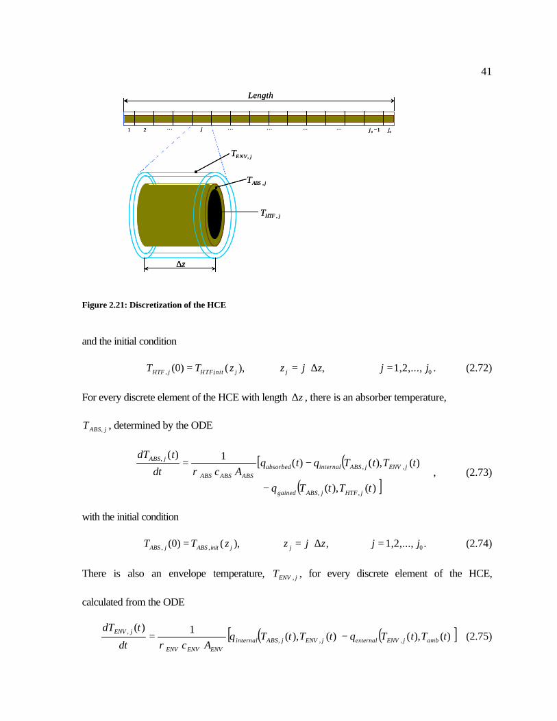
Figure 2.21: Discretization of the HCE

and the initial condition

, , 0(0) ( ), , 1,2,...,HTF j HTFinit j jT T z z j z j j= = ⋅ ∆ = . (2.72)

For every discrete element of the HCE with length z∆ , there is an absorber temperature,

jABST , , determined by the ODE

[ ( )( )])(),(

)(),()(1)(

,,

,,,

tTtTq

tTtTqtqAcdt

tdT

jHTFjABSgained

jENVjABSinternalabsorbedABSABSABS

jABS

−

−=ρ , (2.73)

with the initial condition

, , 0(0) ( ), , 1,2,..., .ABS j ABS init j jT T z z j z j j= = ⋅ ∆ = (2.74)

There is also an envelope temperature, jENVT , , for every discrete element of the HCE,

calculated from the ODE

( ) ( )[ ])(),()(),(1)(

,,,, tTtTqtTtTq

Acdt

tdTambjENVexternaljENVjABSinternal

ENVENVENV

jENV −=ρ

(2.75)

jENVT ,

jABST ,

jHTFT ,

1 2 j 10 −j 0jL L L L L

Length

z∆

jENVT ,

jABST ,

jHTFT ,

1 2 j 10 −j 0jL L L L L

Length

z∆

42with the initial condition

, , 0(0) ( ), , 1,2,...,ENV j ENV i n i t j jT T z z j z j j= = ⋅ ∆ = . (2.76)

The set of ODEs, consisting of equations (2.70), (2.73) and (2.75), and the related initial and

boundary conditions were implemented in the EES (Engineering Equation Solver) simulation

environment (Klein, 2001), together with the model equations for the heat transfer and the

absorbed solar energy discussed above.

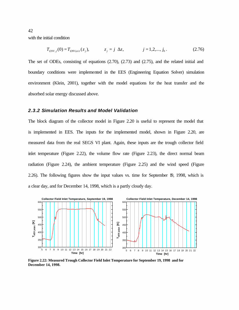
2.3.2 Simulation Results and Model Validation The block diagram of the collector model in Figure 2.20 is useful to represent the model that

is implemented in EES. The inputs for the implemented model, shown in Figure 2.20, are

measured data from the real SEGS VI plant. Again, these inputs are the trough collector field

inlet temperature (Figure 2.22), the volume flow rate (Figure 2.23), the direct normal beam

radiation (Figure 2.24), the ambient temperature (Figure 2.25) and the wind speed (Figure

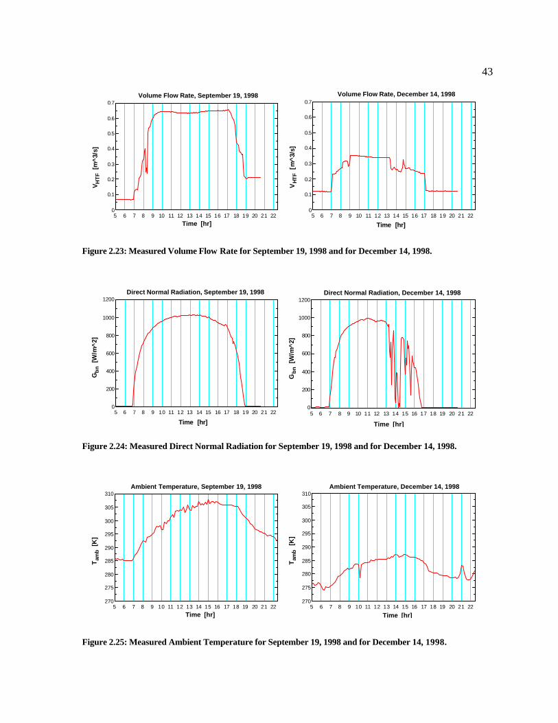
2.26). The following figures show the input values vs. time for September 19, 1998, which is

a clear day, and for December 14, 1998, which is a partly cloudy day.

Figure 2.22: Measured Trough Collector Field Inlet Temperature for September 19, 1998 and for December 14, 1998.

5 6 7 8 9 10 11 12 13 14 15 16 17 18 19 20 21 22300

350

400

450

500

550

600

Time [hr]

TH

TF

,inle

t [K

]

Collector Field Inlet Temperature, September 19, 1998

5 6 7 8 9 10 11 12 13 14 15 16 17 18 19 20 21 22300

350

400

450

500

550

600

Time [hr]

TH

TF

,inle

t [K

]

Collector Field Inlet Temperature, December 14, 1998

43

Figure 2.23: Measured Volume Flow Rate for September 19, 1998 and for December 14, 1998.

Figure 2.24: Measured Direct Normal Radiation for September 19, 1998 and for December 14, 1998.

Figure 2.25: Measured Ambient Temperature for September 19, 1998 and for December 14, 1998.

5 6 7 8 9 10 11 12 13 14 15 16 17 18 19 20 21 220

0.1

0.2

0.3

0.4

0.5

0.6

0.7

Time [hr]

VH

TF [

m^

3/s]

Volume Flow Rate, September 19, 1998

5 6 7 8 9 10 11 12 13 14 15 16 17 18 19 20 21 220

0.1

0.2

0.3

0.4

0.5

0.6

0.7

Time [hr]

VH

TF [

m^

3/s]

Volume Flow Rate, December 14, 1998

5 6 7 8 9 10 11 12 13 14 15 16 17 18 19 20 21 22270

275

280

285

290

295

300

305

310

Time [hr]

Tam

b [

K]

Ambient Temperature, September 19, 1998

5 6 7 8 9 10 11 12 13 14 15 16 17 18 19 20 21 22270

275

280

285

290

295

300

305

310

Time [hr]

Tam

b

[K]

Ambient Temperature, December 14, 1998

5 6 7 8 9 10 11 12 13 14 15 16 17 18 19 20 21 220

200

400

600

800

1000

1200

Time [hr]

Gb

n [

W/m

^2]

Direct Normal Radiation, December 14, 1998

5 6 7 8 9 10 11 12 13 14 15 16 17 18 19 20 21 220

200

400

600

800

1000

1200

Time [hr]

Gb

n [

W/m

^2]

Direct Normal Radiation, September 19, 1998

44

Figure 2.26: Measured Wind Speed for September 19, 1998 and for December 14, 1998.

The trough collector field outlet temperature is calculated through simulations with the model

and compared with measured data of the collector outlet temperature at SEGS VI.

Figure 2.27 shows the calculated collector outlet temperature vs. the measured

collector outlet temperature for June 20, 1998. The calculated values, given through the solid

line, match the measured values, represented by the dashed line, very well. June 20, 1998 is a

clear day with good weather conditions. For another clear day, September 19, 1998, there is

also good agreement between calculated and predicted values (Figure 2.28). The same is true

for December 16, 1998 (Figure 2.29).

Figure 2.30 shows the calculated collector outlet temperature vs. the measured

collector outlet temperature for the partially cloudy day, December 14, 1998. Slight

differences between the calculated and the measured temperatures occur at points where the

slope of the temperature curve changes sign (local temperature minima and maxima).

However, the overall match between the calculated outlet temperature and the measured

outlet temperature is good and verifies that the implemented model is useful as a model for

the real SEGS VI trough collector field.

5 6 7 8 9 10 11 12 13 14 15 16 17 18 19 20 21 220

2

4

6

8

10

12

14

16

Time [hr]

v Win

d [

m/s

]

Wind Speed, September 19, 1998

5 6 7 8 9 10 11 12 13 14 15 16 17 18 19 20 21 220

2

4

6

8

10

12

14

16

Time [hr]

v Win

d [

m/s

]

Wind Speed, December 14, 1998

45

Figure 2.27: Calculated Collector Outlet Temperature vs. Time (solid line) and Measured Collector Outlet Temperature vs. Time (dashed line) on June 20, 1998

Figure 2.28: Calculated Collector Outlet Temperature vs. Time (solid line) and Measured Collector Outlet Temperature vs. Time (dashed line) on September 19, 1998

5 6 7 8 9 10 11 12 13 14 15 16 17 18 19 20 21 22300

350

400

450

500

550

600

650

700

Time [hr]

TH

TF,o

ut

[K]

Collector Outlet Temperature, June 20, 1998

5 6 7 8 9 10 11 12 13 14 15 16 17 18 19 20 21 22300

350

400

450

500

550

600

650

700

Time [hr]

TH

TF,

out

[K]

Collector Outlet Temperature, September 19, 1998

46

Figure 2.29: Calculated Collector Outlet Temperature vs. Time (solid line) and Measured Collector Outlet Temperature vs. Time (dashed line) on December 16, 1998

Figure 2.30: Calculated Collector Outlet Temperature vs. Time (solid line) and Measured Collector Outlet Temperature vs. Time (dashed line) on December 14, 1998

5 6 7 8 9 10 11 12 13 14 15 16 17 18 19 20 21 22300

350

400

450

500

550

600

650

700

Time [hr]

TH

TF,

out

[K]

Collector Outlet Temperature, December 16, 1998

5 6 7 8 9 10 11 12 13 14 15 16 17 18 19 20 21 22300

350

400

450

500

550

600

650

700

Time [hr]

TH

TF

,out

[K

]

Collector Outlet Temperature, December 14, 1998

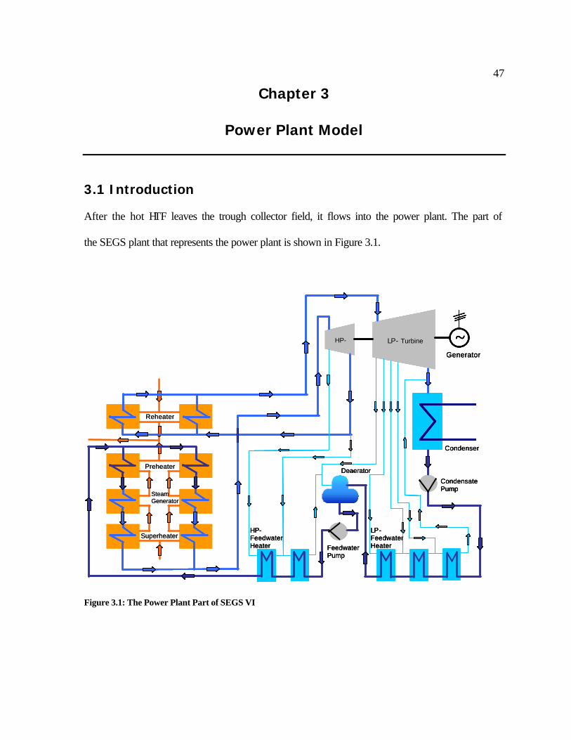
47

Chapter 3

Power Plant Model

3.1 Introduction After the hot HTF leaves the trough collector field, it flows into the power plant. The part of

the SEGS plant that represents the power plant is shown in Figure 3.1.

Figure 3.1: The Power Plant Part of SEGS VI

Reheater

Preheater

SteamGenerator

Superheater

~HP- LP- Turbine

Condenser

Deaerator

HP-FeedwaterHeater

LP-FeedwaterHeater

CondensatePump

FeedwaterPump

Generator

Reheater

Preheater

SteamGenerator

Superheater

~HP- LP- Turbine

Condenser

Deaerator

HP-FeedwaterHeater

LP-FeedwaterHeater

CondensatePump

FeedwaterPump

Generator

~~~HP- LP- Turbine

Condenser

Deaerator

HP-FeedwaterHeater

LP-FeedwaterHeater

CondensatePump

FeedwaterPump

Generator

48Figure 3.1 shows the power plant in pure solar mode. Pure solar mode means that nothing

other than solar energy is used to heat the power plant working fluid. At SEGS VI, an

additional natural-gas-fired boiler is also used to heat the working fluid when no or

insufficient solar energy is available. This combined cycle mode is not considered in this

work and thus the gas-fired boiler is not included in the figure.

The power plant’s working fluid is water or steam. The power plant cycle is a

Clausius-Rankine cycle with feedwater heating, superheating and reheating: the working

fluid leaves the condenser as a condensate and is pressurized by the condensate pump to a

pressure sufficient to pass through the low-pressure feedwater heaters and the deaerator.

Afterwards, the water is heated up in the three low-pressure feedwater heaters through hot

steam extractions withdrawn from the low-pressure turbine. The water then enters the

deaerator (open or direct-contact feedwater heater) where it is mixed with hot steam from the

first extraction of the low-pressure turbine. Through the mixing with steam, the efficient

removal of noncondensables as well as the heating of the water occurs. Since the pressure in

the deaerator cannot exceed the extraction pressure from the first extraction of the low-

pressure turbine, a feedwater pump after the deaerator pumps the water to a higher pressure

to allow the working fluid to pass through the following high-pressure feedwater heaters and

enter the heat exchanger trains. The water is further warmed up in the two high-pressure

feedwater heaters through steam extractions from the high-pressure turbine before it is split

upon entering the two heat exchanger trains. A heat exchanger train consists of a preheater

(economizer), a boiler (steam generator) and a superheater. The water that was warmed up

through feedwater heating enters now the preheater, which is a counterflow heat exchanger,

and is heated by heat exchange with the hot HTF. The working fluid that leaves the preheater

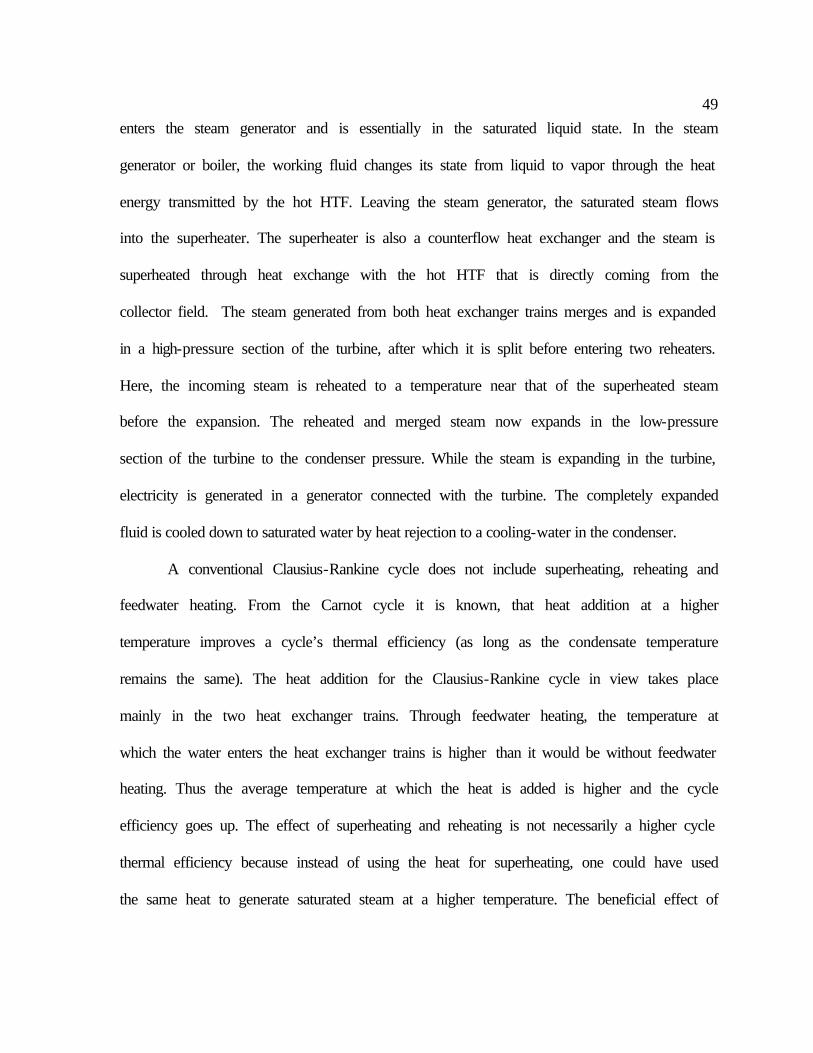
49enters the steam generator and is essentially in the saturated liquid state. In the steam

generator or boiler, the working fluid changes its state from liquid to vapor through the heat

energy transmitted by the hot HTF. Leaving the steam generator, the saturated steam flows

into the superheater. The superheater is also a counterflow heat exchanger and the steam is

superheated through heat exchange with the hot HTF that is directly coming from the

collector field. The steam generated from both heat exchanger trains merges and is expanded

in a high-pressure section of the turbine, after which it is split before entering two reheaters.

Here, the incoming steam is reheated to a temperature near that of the superheated steam

before the expansion. The reheated and merged steam now expands in the low-pressure

section of the turbine to the condenser pressure. While the steam is expanding in the turbine,

electricity is generated in a generator connected with the turbine. The completely expanded

fluid is cooled down to saturated water by heat rejection to a cooling-water in the condenser.

A conventional Clausius-Rankine cycle does not include superheating, reheating and

feedwater heating. From the Carnot cycle it is known, that heat addition at a higher

temperature improves a cycle’s thermal efficiency (as long as the condensate temperature

remains the same). The heat addition for the Clausius-Rankine cycle in view takes place

mainly in the two heat exchanger trains. Through feedwater heating, the temperature at

which the water enters the heat exchanger trains is higher than it would be without feedwater

heating. Thus the average temperature at which the heat is added is higher and the cycle

efficiency goes up. The effect of superheating and reheating is not necessarily a higher cycle

thermal efficiency because instead of using the heat for superheating, one could have used

the same heat to generate saturated steam at a higher temperature. The beneficial effect of

50superheating and reheating, however, is a drier steam at the turbine exhaust that leads to less

erosion at the turbine blades.

The Clausius-Rankine cycle of SEGS VI as described above was modeled in order to

obtain a model of the entire plant. A steady-state model is presented, developed from

measured power plant data and from a report by Lippke on the power plant design conditions

(Lippke, 1995). With the exception of heat exchangers, steady-state models for the power

plant devices seem to be reasonable for the entire plant model since the dynamics of these

systems are much faster compared to the dynamic of the HTF mass circulating in the whole

solar trough collector field.

3.2 Modeling of the Power Plant 3.2.1 Simplifications Before a steady-state model for each part of the power plant is discussed, the Clausius-

Rankine cycle is simplified as shown in Figure 3.2 for easier modeling.

First, the heat exchanger train is considered to be a single heat exchanger instead of

being divided into preheater, steam generator and superheater. It is not assured that the

working fluid’s state between preheater and steam generator and between steam generator

and superheater is defined. This means that the working fluid is not necessarily leaving the

preheater as saturated liquid or entering the superheater as saturated vapor. Treating the heat

exchanger train as a single heat exchanger avoids dealing with this uncertainty. It is now

assumed that pure water is entering the single heat exchanger and superheated steam is

leaving it. But even this assumption may not be satisfied for the start-up period of the plant in

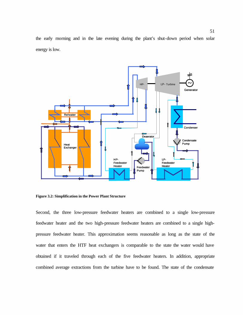
51the early morning and in the late evening during the plant’s shut-down period when solar

energy is low.

Figure 3.2: Simplification in the Power Plant Structure

Second, the three low-pressure feedwater heaters are combined to a single low-pressure

feedwater heater and the two high-pressure feedwater heaters are combined to a single high-

pressure feedwater heater. This approximation seems reasonable as long as the state of the

water that enters the HTF heat exchangers is comparable to the state the water would have

obtained if it traveled through each of the five feedwater heaters. In addition, appropriate

combined average extractions from the turbine have to be found. The state of the condensate

Reheater

~HP- LP- Turbine

Condenser

Deaerator

HP-FeedwaterHeater

LP-FeedwaterHeater

CondensatePump

FeedwaterPump

Generator

HeatExchanger

Reheater

~HP- LP- Turbine

Condenser

Deaerator

HP-FeedwaterHeater

LP-FeedwaterHeater

CondensatePump

FeedwaterPump

Generator

HeatExchanger

52entering the single low-pressure feedwater heater must be comparable to its state in the non-

simplified system as well.

The structure of the simplified power plant is presented again in Figure 3.3, together

with numbers to define the different states in the power plant.

Figure 3.3: Simplified Power Plant Structure

12

3

4

5

6 7

89

10

1112

1314

1516

1718

19

20

21

24

23

22 25

HE A

HE B

RH A

RH B

HPT 1

HPT 2

LPT 1

LPT 2

LPT 3

C

LPFH

HPFH

CP

D

FP

TV 1

TV 212

3

4

5

6 7

89

10

1112

1314

1516

1718

19

20

21

24

23

22 25

HE A

HE B

RH A

RH B

HPT 1

HPT 2

LPT 1

LPT 2

LPT 3

C

LPFH

HPFH

CP

D

FP

TV 1

TV 2

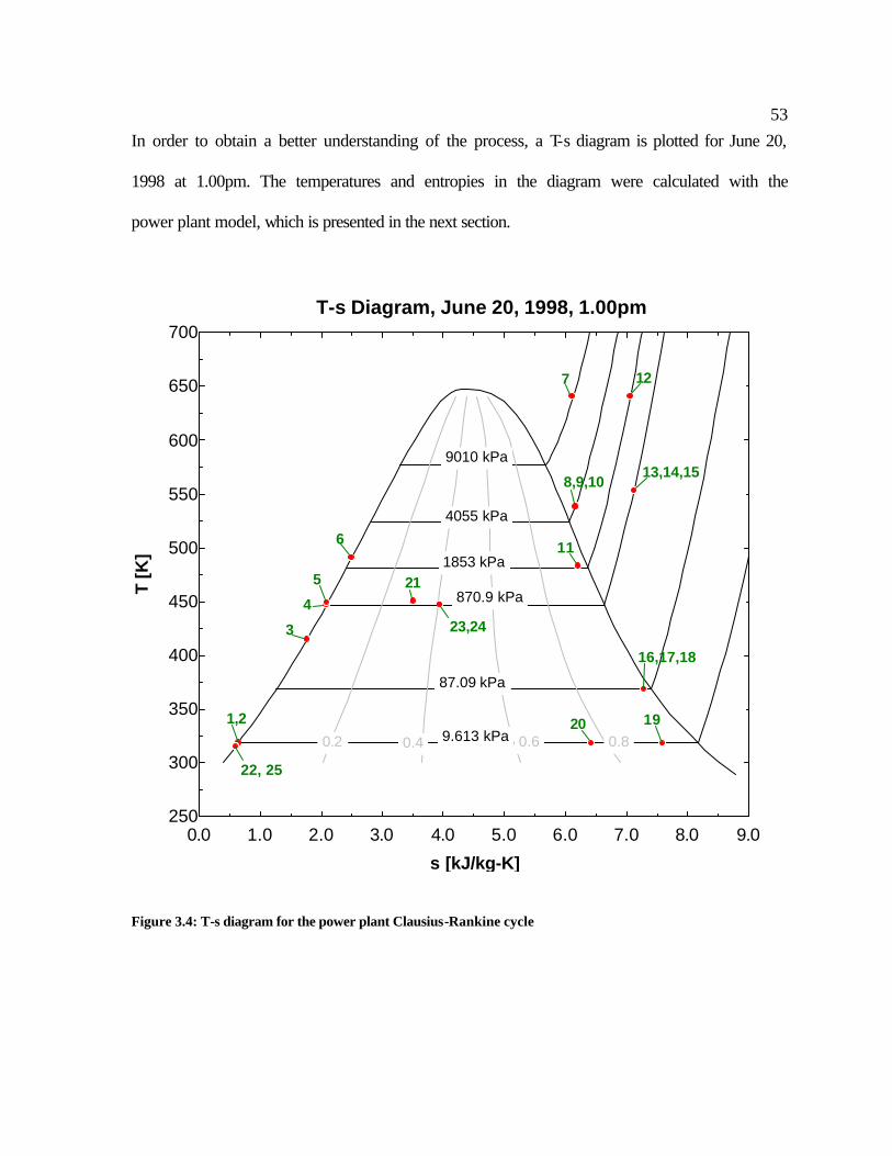
53In order to obtain a better understanding of the process, a T-s diagram is plotted for June 20,

1998 at 1.00pm. The temperatures and entropies in the diagram were calculated with the

power plant model, which is presented in the next section.

Figure 3.4: T-s diagram for the power plant Clausius-Rankine cycle

0.0 1.0 2.0 3.0 4.0 5.0 6.0 7.0 8.0 9.0250

300

350

400

450

500

550

600

650

700

s [kJ/kg-K]

T [K

] 1853 kPa

9010 kPa

4055 kPa

870.9 kPa

87.09 kPa

9.613 kPa 0.2 0.4 0.6 0.8

T-s Diagram, June 20, 1998, 1.00pm

22, 25

1,2

3

4

5

6

7

8,9,10

11

12

13,14,15

16,17,18

1920

23,24

21

54 3.2.2 Modeling 3.2.2.1 Condensate Pump CP and Feedwater Pump FP The pumps are assumed to be adiabatic, but not adiabatic reversible (El-Wakil, 1984). The

internal irreversibility is primarily the result of fluid friction occurring in the pump. Thus the

actual work in CP, 2 1h h− , is greater than the adiabatic reversible work, 2, 1revh h− , - the pump

absorbs more work. The pump irreversibility is represented by a pump isentropic efficiency,

,isCPη , which is given by the ratio of the ideal work to the actual work

2, 1,

2 1

revisCP

h hh h

η−

=−

. (3.1)

The enthalpy, 2,revh , gained if the process would be adiabatic reversible, is calculated from

fluid property functions as the enthalpy of water with the entropy 1s at the pressure 2p :

( )2, 1 2Water, ,rev hh f S s P p= = = . (3.2)

The entropy 1s is known from equation (3.112) and the pressure 2p is calculated through

equation (3.63). The EES inbuilt fluid property functions (Klein, 2001) are used for the

calculation of 2,revh . Since the isentropic efficiency, ,isCPη , is known from Lippke’s report

, 0.7125isCPη = , and the enthalpy 1h is known from equation (3.108), equation (3.1) is used to

calculate the enthalpy 2h . The temperature 2T is also calculated from EES fluid property

functions as the temperature of water with the enthalpy 2h at the pressure 2p

( )2 2 2Water, ,TT f H h P p= = = . (3.3)

55

The entropy 2s is calculated from EES fluid property functions as well. It is the entropy of

water with the enthalpy 2h at the pressure 2p

( )2 2 2Water, ,ss f H h p p= = = . (3.4)

Equations (3.1) – (3.4) define the model for the condensate pump CP. The same calculations

are made for the feedwater pump FP. From Lippke’s report, the isentropic efficiency, ,i s F Pη ,

is the same as for CP, , 0.7125i s F Pη = , and

5, 4,

5 4

revi sFP

h hh h

η−

=−

(3.5)

where the enthalpy 4h is known from equation (3.76). Correspondingly to equation (3.2),

( )5, 4 5Water, ,rev hh f S s P p= = = (3.6)

with the entropy 4s from equation (3.80) and the pressure 5p from equation (3.89). Thus

equation (3.5) is used to calculate the enthalpy 5h . Like for CP, the temperature 5T and the

entropy 5s are calculated from EES fluid property functions

( )5 5 5Water, ,TT f H h P p= = = , (3.7)

( )5 5 5Water, ,ss f H h p p= = = . (3.8)

A mass balance completes the model equations for FP

4 5 0m m− =& & . (3.9)

Through equation (3.9), the mass flow rate 4m& is determined since 5m& is known from

equation (3.85). Equations (3.5) – (3.9) define a model for FP.

In this implementation, a mass balance is not part of the model equations for CP.

Measurements of the mass flow rates in the heat exchanger trains HE A and HE B are

56available. In order to use these measured flow rates as possible inputs to the power plant

model, the mass flow rates in all the different elements of the plant are calculated from

6m& through mass balances for the devices following or preceding the heat exchanger trains

HE A and HE B. Thus 2m& is determined from 3m& through a mass balance for the low-

pressure feedwater heater LPFH, equation (3.61), and 1m& is calculated from 20m& through the

condenser model, equation (3.110). An additional mass balance for CP would have resulted

in an over-determined equation system for the mass flow rates.

3.2.2.2 High-Pressure Turbine HPT 1, HPT 2 and Low-Pressure Turbine LPT 1, LPT 2, LPT 3 Like in pumps, internal irreversibility in turbines is very important. The expansion process is

assumed to be adiabatic, but due to the irreversibility, it is not considered to be adiabatic

reversible (El-Wakil, 1984). For both, the high-pressure section and the low-pressure section

of the turbine, exhaust is to the two-phase region. Hence the entropy increase in the turbine

does not result in a temperature increase but in an increase in enthalpy. Taking the first high-

pressure section of the turbine, HPT 1, as an example, the ideal work through expansion, if

the turbine section were adiabatic reversible, is 7 8,revh h− , but the actual work is 7 8h h− . The

irreversible losses in the turbine are represented by an isentropic efficiency, i.e. for the high-

pressure section, , 1isHPTη .

57It is given by the ratio of the turbine’s actual work to the turbine’s ideal adiabatic reversible

work

7 8, 1

7 8,isHPT

rev

h hh h

η−

=−

. (3.10)

The enthalpy 8,revh is calculated from EES fluid property functions as the enthalpy of steam

with the entropy 7s and the pressure 8p

( )8, 7 8Steam, ,rev hh f S s P p= = = , (3.11)

where the entropy 7s is calculated from equation (3.176) and the pressure 8p is determined

from 7p and a constant pressure ratio, , 1p HPTR ,

8 7 , 1p HPTp p R= ⋅ . (3.12)

The pressure 7p in turn is known from equation (3.174). The enthalpy 7h is calculated from

equation (3.173), hence equation (3.10) is used to determine the enthalpy 8h . The

temperature 8T and the entropy 8s are found through EES fluid property functions as the

temperature and the entropy of steam with the enthalpy 8h at the pressure 8p ,

( )8 8 8Steam, ,TT f H h P p= = = , (3.13)

( )8 8 8Steam, ,ss f H h P p= = = . (3.14)

In order to calculate the mass flow rate 8m& , a mass balance has to be considered

7 8 0m m− =& & . (3.15)

The mass flow rate 7m& is known from equation (3.171).

58Equations (3.10) – (3.15) form the model for the high-pressure section HPT 1 together with

the assumed isentropic efficiency, , 1 0.84i sHPTη = and the assumed constant pressure ratio,

, 1 0.45p HPTR = .

There is a turbine extraction withdrawn between the two high-pressure sections

HPT 1 and HPT 2. This fluid splitting is primarily modeled through the following mass

balance

8 9 10 0m m m− − =& & & . (3.16)

It is assumed that the mass ratio between 9m& and 10m& is known, i.e. from the position of a

splitting valve, and is given as a constant value

9, 1

10mHPT

mR

m= &

&& . (3.17)

For June 20, 1998, the value of , 1mHPTR & is , 1 0.1463mHPTR =& . This value changes for different

days. The split streams are assumed to be in the mechanical and thermodynamic equilibrium:

8 9 10T T T= = , (3.18)

8 9 10p p p= = , (3.19)

8 9 10h h h= = , (3.20)

8 9 10s s s= = . (3.21)

Equations (3.16) – (3.21) describe the model for the extraction splitter between the two high-

pressure turbine sections.

The equations for the turbine sections HPT 2, LPT 1, LPT 2 and LPT 3 are equivalent

to equations (3.10) – (3.15) with the exception that the outlet pressure of the high-pressure

59

turbine part, 11p , and the outlet pressure of the low-pressure turbine part, 19p , are not

calculated from a constant pressure ratio as in equation (3.12). They are rather calculated

from a mass flow rate dependent overall pressure drop, HPp∆ , in the high-pressure part and in

the low-pressure part, LPp∆ of the turbine, where

7

27

0.190594967 0.00141797877

0.0000218417721HPp m

m

∆ = + ⋅

− ⋅

&& , (3.22)

and

12

212

0.00974136866 0.000321840787

0.00000548092767LPp m

m

∆ = − ⋅

+ ⋅

&& . (3.23)

These polynomials are found from measurements of the turbine outlet pressures at different

days. The mass flow rate 12m& is known from equation (3.177).

Thus the set of equations for the turbine section HPT 2 is

10 11, 2

10 11,isHPT

rev

h hh h

η−

=−

, (3.24)

( )11, 10 11Steam, ,revh f S s P p= = = , (3.25)

1011

, 1

HP

p HPT

p pp

R⋅ ∆

= , (3.26)

( )11 11 11Steam, ,TT f H h P p= = = , (3.27)

( )11 11 11Steam, ,ss f H h P p= = = , (3.28)

10 11 0m m− =& & . (3.29)

The isentropic efficiency is assumed to be , 2 0.84isHPTη = .

60There exists a similar set of equations for the first low-pressure turbine section LPT 1:

12 13, 1

12 13,isLPT

rev

h hh h

η−

=−

, (3.30)

where the enthalpy 12h is known from equation (3.179). Similarly to equation (3.11), it is

( )13, 12 13Steam, ,rev hh f S s P p= = = , (3.31)

with the entropy 12s from equation (3.182).

The pressure 13p is determined from

13 12 , 1pLPTp p R= ⋅ , (3.32)

where the pressure 12p is known from equation (3.180). The pressure ratio 1,LPTpR is

assumed to be constant with 47.01, =LPTpR . The remaining equations are

( )13 13 13Steam, ,TT f H h P p= = = , (3.33)

( )13 13 13Steam, ,ss f H h P p= = = , (3.34)

12 13 0m m− =& & . (3.35)

The isentropic efficiency is assumed to be , 1 0.8376isLPTη = .

The turbine extraction between the first low-pressure section LPT 1 and the second

low-pressure section LPT 2 can be modeled equivalently to equations (3.16) – (3.21):

13 14 15 0m m m− − =& & & . (3.36)

14, 1

15mLPT

mR

m= &

&& . (3.37)

13 14 15T T T= = , (3.38)

13 14 15p p p= = , (3.39)

61

13 14 15h h h= = , (3.40)

13 14 15s s s= = . (3.41)

For June 20, 1998, the value of the mass ratio is , 1 0.02mLPTR =& .

The set of equations for the second low-pressure section of the turbine, LPT 2, is

15 16, 2

15 16,isLPT

rev

h hh h

η−

=−

, (3.42)

( )16, 15 16Steam, ,rev hh f S s P p= = = , (3.43)

16 15 , 2pLPTp p R= ⋅ , (3.44)

( )16 16 16Steam, ,TT f H h P p= = = , (3.45)

( )16 16 16Steam, ,ss f H h P p= = = , (3.46)

15 16 0m m− =& & . (3.47)

The isentropic efficiency is assumed to be , 2 0.8623isLPTη = and the assumed constant

pressure ratio is , 2 0.1p LPTR = .

The turbine extraction between the second low-pressure section LPT 2 and the third

low-pressure section LPT 3 is similarly modeled as above:

16 17 18 0m m m− − =& & & . (3.48)

17, 2

18mLPT

mR

m= &

&& . (3.49)

16 17 18T T T= = , (3.50)

16 17 18p p p= = , (3.51)

16 17 18h h h= = , (3.52)

62

16 17 18s s s= = . (3.53)

For June 20, 1998, the value of the mass ratio is , 2 0.2mLPTR =& .

Finally, the model equations for the last low-pressure turbine section, LPT 3, is given

through

18 19, 3

18 19,isLPT

rev

h hh h

η−

=−

, (3.54)

( )19, 18 19Steam, ,rev hh f S s P p= = = , (3.55)

1819

, 1 , 2

LP

pLPT pLPT

p pp

R R⋅ ∆

=⋅

, (3.56)

( )19 19 19Steam, ,TT f H h P p= = = , (3.57)

( )19 19 19Steam, ,ss f H h P p= = = , (3.58)

18 19 0m m− =& & . (3.59)

The isentropic efficiency is assumed to be , 3 0.7isLPTη = .

3.2.2.3 Low-Pressure Feedwater Heater LPFH The low-pressure feedwater heater, LPFH, is a closed-type feedwater heater with a backward

drain. Feedwater heaters are usually shell-and-tube heat exchangers (El-Wakil, 1984) and

since no information on the LPFH at SEGS VI was available, it is assumed to be a shell-and-

tube heat exchanger as well. The feedwater passes through the tubes and the bled steam that

comes from the turbine extraction between LPT 2 and LPT 3, is on the shell side and

transfers its energy to the feedwater.

63Thus an energy balance between the bled steam and the feedwater is the first equation for the

LPFH model

2 2 3 3 17 17 22 22 0m h m h m h m h− + − =& & & & . (3.60)

This equation determines the drain enthalpy 22h since the enthalpy 2h is known from equation

(3.1), the enthalpy 3h is calculated with equation (3.82) and the enthalpy of the bled steam,

17h , is known from equation (3.52). The steam mass flow rate, 17m& , is calculated from

equation (3.48) and (3.49). The feedwater mass flow rate, 2m& , is determined from the

following mass balance that is part of the LPFH model

2 3 0m m− =& & . (3.61)

The mass flow rate 3m& comes from equation (3.81). The drain stream leaves the LPFH with

the mass flow rate 22m& from

17 22 0m m− =& & . (3.62)

Pressure drops of the feedwater in feedwater heaters are usually large because of the flow

friction in long small-diameter tubes. For the LPFH in view, the pressure 2p is given through

3 2 LPFHp p p= ⋅ ∆ (3.63)

where 0.5LPFHp∆ = is assumed to be constant. The pressure 3p is known from equation

(3.78). The temperature 3T and the entropy 3s are found through EES fluid property

functions as the temperature and the entropy of water with the enthalpy 3h at the pressure 3p ,

( )3 3 3Water, ,TT f H h P p= = = , (3.64)

( )3 3 3Water, ,ss f H h P p= = = . (3.65)

64Equations (3.60) – (3.65) form the model for the low-pressure feedwater heater LPFH.

3.2.2.4 Deaerator D and Throttle Valve TV 1 The deaerator D is an open- or direct-contact feedwater heater where the extraction steam is

mixed directly with the incoming feedwater to produce saturated water at the extraction

steam pressure (El-Wakil, 1984). Before it enters D, the extraction steam that is withdrawn

between LPT 1 and LPT 2, is mixed with the drain stream of the high-pressure feedwater

heater HPFH. The higher pressured drain stream passes a throttle valve to reduce its pressure

to the pressure of the turbine extraction steam before the two streams merge. The pressure of

the turbine extraction steam, 14p , is calculated from equation (3.39) and thus

24 14p p= (3.66)

defines the outlet pressure of TV 1. No heat losses are assumed for TV 1, hence

24 21h h= (3.67)

and the temperature is assumed to stay constant:

24 21T T= . (3.68)

The drain enthalpy 21h is calculated from equation (3.86) and the drain temperature 21T is

known from equation (3.93). A mass balance on TV 1 yields

21 24 0m m− =& & , (3.69)

where the drain mass flow rate, 21m& , comes from equation (3.84).

65

The outlet entropy of TV1, 24s , is calculated with EES fluid property functions as the

entropy of steam with the enthalpy 24h at the pressure 24p :

( )242424 ,,Steam pPhHfs s === . (3.70)

Equations (3.66) – (3.70) are the TV 1 model equations.

The throttle’s outlet stream merges with the extraction steam of the turbine. Thus the

fluid that enters D at the steam side has the mass flow rate 23m& from

14 24 23 0m m m+ − =& & & . (3.71)

The extraction mass flow rate 14m& is known from equations (3.36) and (3.37). The enthalpy

of the steam entering D, 23h , is determined from the following energy balance

14 14 24 24 23 23 0m h m h m h+ − =& & & , (3.72)

where the extraction steam enthalpy, 14h , is known from equation (3.40). The merging

streams are in a mechanical equilibrium and hence

23 14p p= . (3.73)

The steam-side inlet temperature, 23T , is calculated with EES fluid property functions as the

temperature of steam with enthalpy 23h at the pressure 23p :

( )23 23 23Steam, ,TT f H h P p= = = . (3.74)

The steam-side inlet entropy, 23s , is also calculated with EES fluid property functions as the

entropy of steam with the enthalpy 23h at the pressure 23p :

( )232323 ,,Steam pPhHfs s === . (3.75)

66Equations (3.71) – (3.75) form the model equations for the merging of the turbine extraction

stream with the HPFH drain stream.

The deaerator is supposed to produce saturated feedwater at the extraction steam

pressure. Thus the enthalpy of the saturated feedwater, 4h , is calculated from EES fluid

property functions as the enthalpy of saturated water at the pressure 23p :

( )4 23Steam, , 0hh f P p X= = = . (3.76)

This assumption includes that the feedwater outlet pressure of D, 4p , is the same as the

steam inlet pressure 23p ,

4 23p p= . (3.77)

In addition, no pressure drop in the feedwater is assumed

3 4p p= . (3.78)

Thus the feedwater outlet temperature, 4T , can be calculated from EES property functions as

the temperature of steam with the enthalpy 4h at the pressure 4p ,

( )4 4 4Steam, ,TT f H h P p= = = . (3.79)

Also the feedwater outlet entropy, 4s , is calculated from fluid property functions as the

entropy of steam with the enthalpy 4h at the pressure 4p ,

( )4 4 4Steam, ,ss f H h P p= = = . (3.80)

A mass balance on D has to account for the fact that the feedwater inlet stream and the steam

inlet stream are mixed together and form the feedwater outlet stream. The feedwater inlet

stream has the mass flow rate 3m& from

3 23 4 0m m m+ − =& & & , (3.81)

67

where the mass flow rate 4m& is known from equation (3.9) and the steam mass flow rate 23m&

is determined from equation (3.71). The following energy balance is used to find a value for

the feedwater inlet enthalpy, 3h ,

3 3 23 23 4 4 0m h m h m h+ − =& & & . (3.82)

Equations (3.76) – (3.82) form the model equations for the deaerator D.

3.2.2.5 High-Pressure Feedwater Heater HPFH The high-pressure feedwater heater HPFH is like the LPFH a closed-type feedwater heater

with a backward drain. Assuming again a shell-and-tube heat exchanger (El-Wakil, 1984), an

energy balance is established between the bled steam and the feedwater

5 5 6 6 9 9 21 21 0m h m h m h m h− + − =& & & & . (3.83)

Through this equation, the feedwater outlet enthalpy, 6h , is calculated since the extraction

enthalpy, 9h , is determined from equation (3.20) and the feedwater inlet enthalpy, 5h , is

given through equation (3.5). The extraction mass flow rate, 9m& , is calculated from equations

(3.16) and (3.17). The drain mass flow rate, 21m& , follows from

9 21 0m m− =& & . (3.84)

The feedwater mass flow rate, 5m& , is determined from the following mass balance for the

feedwater

5 6 0m m− =& & (3.85)

where the mass flow rate 6m& is an input of the power plant model.

68

The drain enthalpy, 21h , is calculated from an effectiveness equation for HPFH

9 21

9 5HPFH

h hh h

ε−

=−

, (3.86)

From measurements of the water inlet conditions and steam outlet conditions of the heat

exchanger trains A and B (HE A and HE B), it seems that the effectiveness, HPFHε , is a

function of the fraction of the two inlet mass flow rates, 9

5

mm&& , and of the feedwater mass flow

rate, 5m& , itself. From Lippke’s report, design values of the two mass flow rates are given.

They are 50 38.969 kg/sm =& and 90 5.7319 kg/sm =& . These design values are used to define

the following variable

9 5 5

90 50 50

/12 /

m m mB

m m m

= +

& & && & & , (3.87)

that is used to estimate the effectiveness, HPFHε , from the following polynomial

2 3

0.433509942 1.72903764

3.21718006 1.29319762HPFH B

B B

ε = − ⋅

+ ⋅ − ⋅. (3.88)

This polynomial was found through fitting measured heat exchanger train inlet water data

when measured heat exchanger train outlet steam data were used as model inputs.

A constant pressure drop is considered in the feedwater and also at the steam side of

the HPFH

6 5 ,HPFH cp p p= ⋅ ∆ , (3.89)

21 9 ,HPFH hp p p= ⋅ ∆ . (3.90)

Estimated from Lippke’s report, the values for the pressure ratios are , 0.8286HPFH cp∆ = and

, 0.236HPFH hp∆ = . Equation (3.89) gives a value for the feedwater inlet pressure 5p , since the

69

feedwater outlet pressure, 6p , is known from equation (3.126). Correspondingly, equation

(3.90) yields a value for the drain pressure 21p , since the extraction pressure, 9p , is known

from equation (3.19). The feedwater outlet temperature, 6T , and the feedwater outlet entropy,

6s , are calculated from fluid property functions as the temperature and entropy of water with

the enthalpy 6h at the pressure 6p :

( )6 6 6Water, ,TT f H h P p= = = , (3.91)

( )6 6 6Water, ,ss f H h P p= = = . (3.92)

Likewise, the drain temperature, 21T , and the drain entropy, 21s , are calculated from fluid

property functions as the temperature and entropy of steam with the enthalpy 21h at the

pressure 21p :

( )21 21 21Steam, ,TT f H h P p= = = , (3.93)

( )21 21 21Steam, ,ss f H h P p= = = . (3.94)

Equations (3.83) – (3.94) define the model for the high-pressure feedwater heater HPFH.

3.2.2.6 Condenser C and Throttle Valve TV 2 The condenser C is primarily a heat-transfer equipment with the purpose to condense the

exhaust steam from the low-pressure part of the turbine and thus recover the high-quality

feedwater for reuse in the cycle (El-Wakil, 1984). Before the turbine exhaust enters the

condenser, it is mixed with the drain stream of the low-pressure feedwater heater LPFH. This

drain stream passes a throttle valve TV 2 before it is mixed with the exhaust stream. Since

70

the mixing streams are in a mechanical equilibrium, the throttle valve’s outlet pressure, 25p ,

is the same as the exhaust pressure

25 19p p= . (3.95)

The turbine exhaust pressure, 19p , is determined by equation (3.56). The pressure drop

induced by TV 2 is given through

25 22 2TVp p p= ⋅ ∆ , (3.96)

where the pressure ratio is estimated to 2 0.57TVp∆ = . This equation is used to calculate the

LPFH drain pressure, 22p . This pressure is used to calculate the LPFH drain temperature,

22T , and the drain entropy, 22s , from fluid property functions as the temperature and entropy

of steam with the enthalpy 22h at the pressure 22p :

( )22 22 22Steam, ,TT f H h P p= = = , (3.97)

( )22 22 22Steam, ,ss f H h P p= = = . (3.98)

The drain enthalpy, 22h , is known from equation (3.60). The enthalpy stays constant in the

adiabatic throttle valve TV 2

25 22h h= . (3.99)

In addition, a constant temperature is assumed

25 22T T= . (3.100)

There is no loss of mass in TV 2, hence

22 25 0m m− =& & . (3.101)

71

The mass flow rate 22m& is calculated from equation (3.62). The entropy of the throttle valve’s

outlet stream is calculated from fluid property functions as the entropy of steam with the

enthalpy 25h at the pressure 25p :

( )25 25 25Steam, ,s f H h P p= = = . (3.102)

Equations (3.95) – (3.102) form the model equations for the throttle valve TV 2.

Before entering the condenser, the throttled drain stream is mixed with the low-

pressure turbine exhaust. This fact is described through the following mass balance

19 25 20 0m m m+ − =& & & . (3.103)

This equation is used to calculate the mass flow rate 20m& since the exhaust mass flow rate

19m& is known from equation (3.59). The fluid entering C is in a mechanical equilibrium with

the merging streams and thus

20 19p p= . (3.104)

The enthalpy of the fluid that enters the condenser C, 20h , is determined from the following

energy balance

19 19 25 25 20 20 0m h m h m h+ − =& & & . (3.105)

The enthalpy of the exhaust, 19h , is known from equation (3.54). The temperature 20T is

calculated from fluid property functions as the temperature of steam with the enthalpy 20h at

the pressure 20p

( )20 20 20Steam, ,TT f H h P p= = = . (3.106)

72

The entropy 20s is also calculated from fluid property functions as the entropy of steam with

the enthalpy 20h at the pressure 20p :

( )20 20 20Steam, ,ss f H h P p= = = . (3.107)

Equations (3.103) – (3.107) define the model for the mixing of the turbine exhaust with the

LPFH drain stream.

The mixed fluid enters the condenser and looses its energy to the circulating cooling

water until it leaves the condenser as saturated liquid. Thus the enthalpy of the outlet flow,

1h , is assumed to be the enthalpy of saturated water at the pressure 20p and is calculated

from fluid property functions:

( )1 20Steam, , 0hh f P p X= = = . (3.108)

Hence the pressure is assumed to remain constant

1 20p p= , (3.109)

and the mass flow rate stays constant as well

20 1 0m m− =& & . (3.110)

The outlet temperature 1T and the entropy 1s are calculated from EES fluid property

functions as the temperature and the entropy of steam with the enthalpy 1h at the pressure

1p :

( )1 1 1Steam, ,TT f H h P p= = = , (3.111)

( )1 1 1Steam, ,ss f H h P p= = = . (3.112)

The incoming cooling water temperature, ,C o o l iT , is one of the inputs to the power plant model

but does not affect the enthalpy 1h in this implementation due to the assumption of saturated

73liquid outlet conditions in equation (3.108). The pressure of the incoming cooling water,

,C o o l ip , is assumed to be the ambient pressure

,Cooli atmp p= . (3.113)

From fluid property functions, the cooling water inlet enthalpy, ,C o o l ih , is calculated as the

enthalpy of water with the temperature ,C o o l iT at the pressure ,C o o l ip

( ), , ,Water, ,Cool i Cool i C o o l ih f T T P p= = = . (3.114)

There is no pressure drop assumed in the cooling water and the cooling water outlet pressure,

,C o o l op , is

, ,Cool o C o o l ip p= , (3.115)

Also the mass flow rate of the cooling water remains constant

, , 0Cool i C o o l om m− =& & , (3.116)

where ,C o o l om& is the cooling water outlet mass flow rate and ,C o o l im& is the mass flow rate of

the incoming cooling water and is estimated to be proportional to the heat exchanger train

inlet mass flow rate, 6m& :

, 639.38C o o l im m= ⋅& & . (3.117)

The factor 39.38 was determined from measurements of the cooling water outlet temperature

to satisfy the following energy balance

( ) ( ), , , 20 20 1Cool i Coolo C o o l im h h m h h− = −& & . (3.118)

74

From this equation, the cooling water outlet enthalpy ,C o o l oh is calculated. From this enthalpy,

the temperature of the outlet cooling water, ,C o o l oT , is determined from fluid property

functions as the temperature of water with the enthalpy ,C o o l oh at the pressure ,C o o l op :

( ), , ,Water, ,Coolo T Coolo Cool oT f H h P p= = = . (3.119)

Equations (3.108) – (3.119) define model for the condenser C.

3.2.2.7 Heat Exchanger Train HE A and HE B and Reheater RH A and RH B The heat exchanger trains HE A and HE B and the reheaters RH A and RH B are very

important parts of the power plant since they represent the interface between the HTF cycle

and the power plant cycle. The heat transfer between the HTF and the working fluid of the

power plant occurs in these heat exchangers.

From the HTF side, the HTF is split into two streams where one stream flows into the

heat exchanger trains and the other stream flows into the reheaters. From the pipe geometry,

the amount of HTF that flows into the reheaters cannot exceed 25% of the entire HTF that

leaves the expansion vessel. However, the splitting fraction that is not measured in the plant

differs from operator to operator. As an approximate value for the splitting fraction, the

design values from Lippke’s report are used in this approach (Lippke, 1995). The HTF splits

evenly between the two heat exchanger trains HE A and HE B. The same is true for the two

reheaters RH A and RH B. The HTF that leaves the expansion vessel is split into a stream of

fraction Aa that flows into HE A, into a stream of fraction Ba that flows into HE B, into a

stream of fraction Ab that flows into RH A and finally into a stream of fraction Bb that flows

75

into RH B. From Lippke’s report, the design values of these fractions are 0.4375A Ba a= =

and 0.0625A Bb b= = .

There is also splitting at the water or steam side. The feedwater of fraction H E AF

enters HE A. The remaining part of the feedwater with fraction H E BF enters HE B and

1HEB H E AF F= − . (3.120)

These fractions may differ from day to day. At June 20, 1998, the feedwater fraction for HE

A is 0.49H E AF = . There is also splitting occurring in front of the reheaters. The expanded

steam flows into RH A with fraction R H AF and R H BF is the fraction determining the steam

that enters RH B.

Correspondingly,

1RHB R H AF F= − . (3.121)

At June 20, 1998, the fraction for RH A is 0.53RHAF = .

From the definition of the flow fractions, it follows the mass flow rates

6HEA H E Am F m= ⋅& & , (3.122)

6HEB H E Bm F m= ⋅& & . (3.123)

Here, HEAm& is the mass flow rate of the fluid that passes through HE A and HEBm& is the mass

flow rate of the fluid that passes through HE B. The mass flow rate of the feedwater that

enters the heat exchanger trains, 6m& , is an input to the power plant model. Measurements

from the real SEGS VI plant of that value are available. These measurements can be used as

possible inputs for simulations with the power plant model. The pressures H E Ap and H E Bp

76that develop in the two heat exchanger trains HE A and HE B respectively, are functions of

the mass flow rates HEAm& and HEBm& . The polynomials were found from measurements of the

mass flow rate and the pressure at SEGS VI:

2

3 4

1373.83964 374.607738 128.736553

8.0075749 0.177361045HEA HEA H E A

H E A HEA atm

p m m

m m p

= − ⋅ + ⋅

− ⋅ + ⋅ +

& && & , (3.124)

2

683.996786 343.994696

4.56017193

HEB H E B

HEB atm

p m

m p

= + ⋅

+ ⋅ +

&& . (3.125)

From these two pressures, the pressure of the feedwater that enters the two heat exchanger

trains, 6p , is calculated as

6 HEA HEA HEB H E Bp F p F p= ⋅ + ⋅ . (3.126)

The feedwater temperature 6T is determined from equation (3.91). The temperatures of the

two feedwater streams into HE A and HE B, ,Water H E AT and ,Water H E BT , are assumed to be the

same as 6T

, 6WaterHEAT T= , (3.127)

, 6WaterHEBT T= . (3.128)

Equations (3.122) – (3.128) model the splitting of the feedwater into the two heat exchanger

train’s inlet flows.

The exhaust steam from the high-pressure part of the turbine is also split two enter the

two reheaters RH A and RH B. Thus similar equations can be found. The mass flow rates are

11R H A R H Am F m= ⋅& & , (3.129)

11R H B R H Bm F m= ⋅& & , (3.130)

77

where the exhaust mass flow rate, 11m& , is found from equation (3.29). From measurements on

the real power plant, it can be seen that a pressure drop occurs in the steam on its way from

the high-pressure turbine outlet to the two reheaters RH A and RH B. Thus the two pressures

R H Ap and R H Bp that develop in RH A and RH B respectively, are determined from the

exhaust pressure 11p as

11R H A R H Ap p p= ⋅ ∆ , (3.131)

11RHB R H Bp p p= ⋅ ∆ . (3.132)

The pressure 11p is known from equation (3.26). The two pressure ratios R H Ap∆ and R H Bp∆

are functions of the two mass flow rates R H Am& and R H Bm& . These functions are polynomials

found through a curve fit on the measured data from SEGS VI

2

1.03315016 0.00615276988

0.000167339399

R H A R H A

R H A

p m

m

∆ = − ⋅

+ ⋅

&& , (3.133)

2

1.01609492 0.00408501006

0.0000767853121

R H B R H B

R H B

p m

m

∆ = − ⋅

+ ⋅

&& . (3.134)

The temperature of the fluid that enters RH A, , ,S t e a m R H A iT , and the temperature of the fluid

that enters RH B, , ,S t e a m R H B iT , is assumed to match the temperature of the high-pressure

turbine exhaust 11T and thus

, , 11S t e a m R H A iT T= , (3.135)

, , 11S t e a m R H B iT T= . (3.136)

Equations (3.129) – (3.136) model the splitting of the high-pressure turbine exhaust into the

two streams entering RH A and RH B.

78The HTF that leaves the expansion vessel is split into the parts that enter HE A, HE B, RH A

and RH B as explained above. The temperature of the four split HTF streams that enter the

heat exchangers and reheaters are assumed to have the expansion vessel temperature, ExpT .

The four streams leave the heat exchangers and reheaters, each with its own HTF outlet

temperature, and merge to form the inlet flow of the solar trough collector field. The HTF

outlet temperature for HE A is ,HTF H E AT , the HTF outlet temperature for HE B is ,HTF H E BT , the

HTF outlet temperature for RH A is ,HTF R H AT and the HTF outlet temperature for RH B is

,HTF R H BT . Since no HTF mass is lost on its way through HE A, HE B, RH A and RH B, the

HTF inlet temperature of the solar trough collector field, ,HTFinletT , is calculated from the flow

fractions defined above:

, , , , ,HTFinlet A HTF HEA B HTF HEB A HTF R H A B HTF R H BT a T a T b T b T= + + + . (3.137)

Since the overall HTF volume flow rate, HTFV& , is available as measurement data from the real

SEGS VI plant, it is used together with the flow fractions to calculated the heat that is

transferred to the working fluid in the different heat exchangers and reheaters:

( ),H E A A HTF HTF HTF Exp HTF HEAQ a c V T Tρ= −& & , (3.138)

( ),HEB B HTF HTF HTF Exp HTF HEBQ a c V T Tρ= −& & , (3.139)

( ),R H A A HTF HTF HTF Exp HTF R H AQ b c V T Tρ= −& & , (3.140)

( ),R H B B HTF HTF HTF Exp HTF R H BQ b c V T Tρ= −& & . (3.141)

To predict the outlet temperatures of the HTF, the log mean temperature difference for

counterflow with an overall heat transfer coefficient is applied as a common calculation

79method for heat exchangers. From Incropera & DeWitt (2001), the heat in equations (3.138)

– (3.141) is balanced with

( ),1 ,2

,1 ,2ln /HEA H E A

H E A H E AH E A H E A

T TQ UA

T T

∆ − ∆=

∆ ∆& , (3.142)

( ),1 ,2

,1 ,2ln /HEB H E B

HEB H E BHEB H E B

T TQ UA

T T

∆ − ∆=

∆ ∆& , (3.143)

( ),1 ,2

,1 ,2ln /R H A R H A

R H A R H AR H A R H A

T TQ UA

T T

∆ − ∆=

∆ ∆& , (3.144)

( ),1 ,2

,1 ,2ln /RHB R H B

R H B R H BR H B R H B

T TQ UA

T T

∆ − ∆=

∆ ∆& . (3.145)

In these equations, the temperature differences are

,1 ,H E A Exp SteamHEAT T T∆ = − , (3.146)

,2 , ,H E A HTF H E A Water H E AT T T∆ = − , (3.147)

,1 ,HEB Exp SteamHEBT T T∆ = − , (3.148)

,2 , ,HEB HTF HEB Water H E BT T T∆ = − , (3.149)

,1 , ,R H A Exp S t e a m R H A oT T T∆ = − , (3.150)

,2 , , ,R H A HTF R H A Steam R H A iT T T∆ = − , (3.151)

,1 , ,R H B Exp S t e a m R H B oT T T∆ = − , (3.152)

,2 , , ,R H B HTF R H B Steam R H B iT T T∆ = − , (3.153)

where ,SteamHEAT is the working fluid outlet temperature of HE A, and ,SteamHEBT , , ,S t e a m R H A oT

and , ,S t e a m R H B oT are the working fluid outlet temperatures of HE B, RH A and RH B

80respectively. The overall heat transfer coefficients are different from heat exchanger to heat

exchanger. They depend on the mass flow rate of the HTF and the mass flow rate of the

working fluid. Since the overall HTF volume flow rate, HTFV& , and the mass flow rate 6m& of

the working fluid are available as measured data, the following variable is defined that is

equally dependent on the HTF volume flow rate and the mass flow rate:

6

,0 6,0

12

HTF

HTF

mVM

V m

= +

& && & . (3.154)

Here, 30 0.624 m /sV =& and 6,0 39.9 kg/sm =& are the values of the HTF volume flow rate and

the mass flow rate at solar noon on June 20, 1998. The variable M is used to find expressions

for the different overall heat transfer coefficient-area products:

2 3

792.404548 5631.66157

5732.19845 2201.04063H E AUA M

M M

= − + ⋅

− ⋅ + ⋅, (3.155)

2 3

1460.34016 8693.5446

10858.5127 4905.3059HEBUA M

M M

= − + ⋅

− ⋅ + ⋅, (3.156)

28217.68129 92925.7393 168323.253R H AUA M M= − + ⋅ + ⋅ , (3.157)

213356.4707 68312.7678 348273.243R H BUA M M= − ⋅ + ⋅ . (3.158)

These polynomials were found through a curve fit on overall heat transfer coefficients that

were calculated from measurement data and plotted vs. M. From equations (3.138) – (3.158),

the HTF outlet temperatures ,HTF H E AT , ,HTF H E BT , ,HTF R H AT and ,HTF R H BT could be determined if

the working fluid outlet temperatures, ,SteamHEAT , ,SteamHEBT , , ,S t e a m R H A oT and , ,S t e a m R H B oT were

known. In order to calculate the working fluid outlet temperatures, an energy balance would

be preferable, but since the flow fractions Aa , Ba , Ab and Bb are uncertain, a heat exchanger

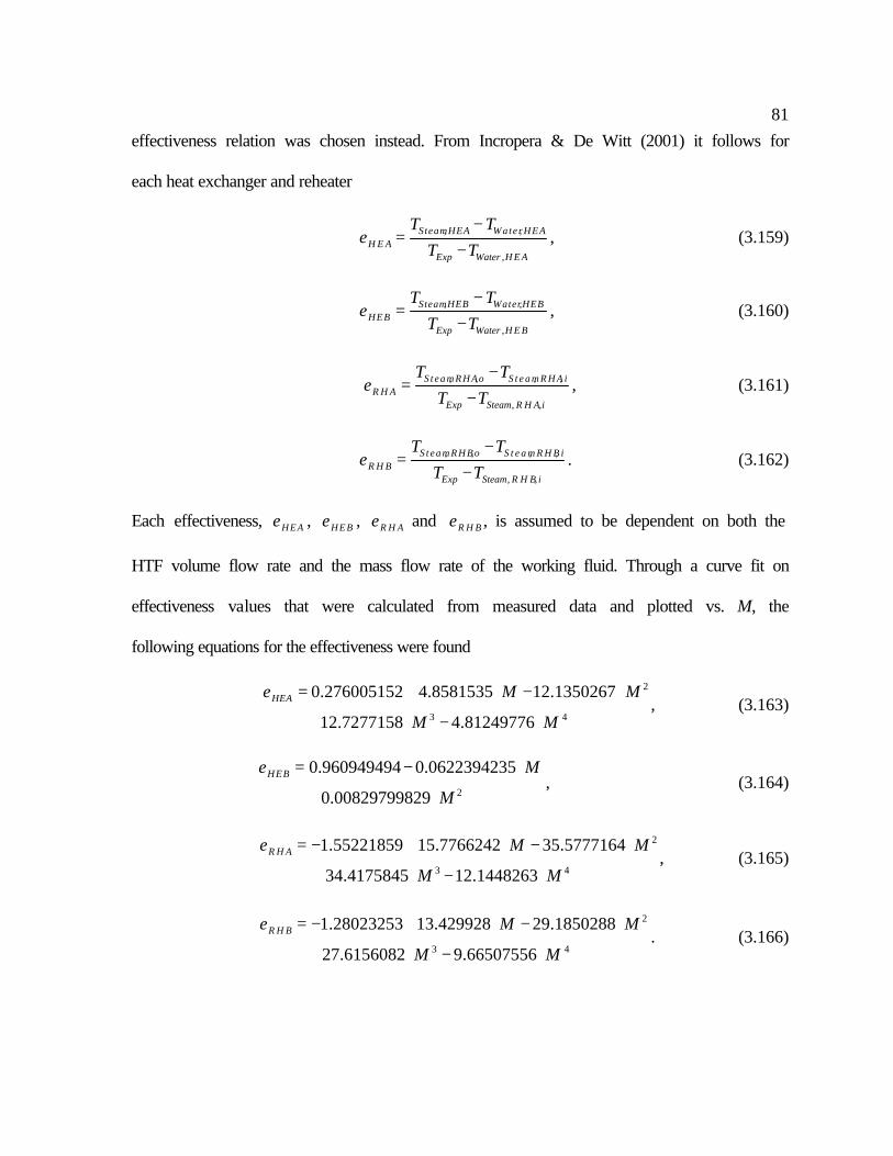
81effectiveness relation was chosen instead. From Incropera & De Witt (2001) it follows for

each heat exchanger and reheater

, ,

,

SteamHEA WaterHEAH E A

Exp Water H E A

T TT T

ε−

=−

, (3.159)

, ,

,

SteamHEB WaterHEBHEB

Exp Water H E B

T TT T

ε−

=−

, (3.160)

, , , ,

, ,

S t e a m R H A o S t e a m R H A iR H A

Exp Steam R H A i

T TT T

ε−

=−

, (3.161)

, , , ,

, ,

S t e a m R H B o S t e a m R H B iR H B

Exp Steam R H B i

T TT T

ε−

=−

. (3.162)

Each effectiveness, HEAε , HEBε , R H Aε and R H Bε , is assumed to be dependent on both the

HTF volume flow rate and the mass flow rate of the working fluid. Through a curve fit on

effectiveness values that were calculated from measured data and plotted vs. M, the

following equations for the effectiveness were found

2

3 4

0.276005152 4.8581535 12.1350267

12.7277158 4.81249776HEA M M

M M

ε = + ⋅ − ⋅

+ ⋅ − ⋅, (3.163)

2

0.960949494 0.0622394235

0.00829799829HEB M

M

ε = − ⋅

+ ⋅, (3.164)

2

3 4

1.55221859 15.7766242 35.5777164

34.4175845 12.1448263R H A M M

M M

ε = − + ⋅ − ⋅

+ ⋅ − ⋅, (3.165)

2

3 4

1.28023253 13.429928 29.1850288

27.6156082 9.66507556R H B M M

M M

ε = − + ⋅ − ⋅

+ ⋅ − ⋅. (3.166)

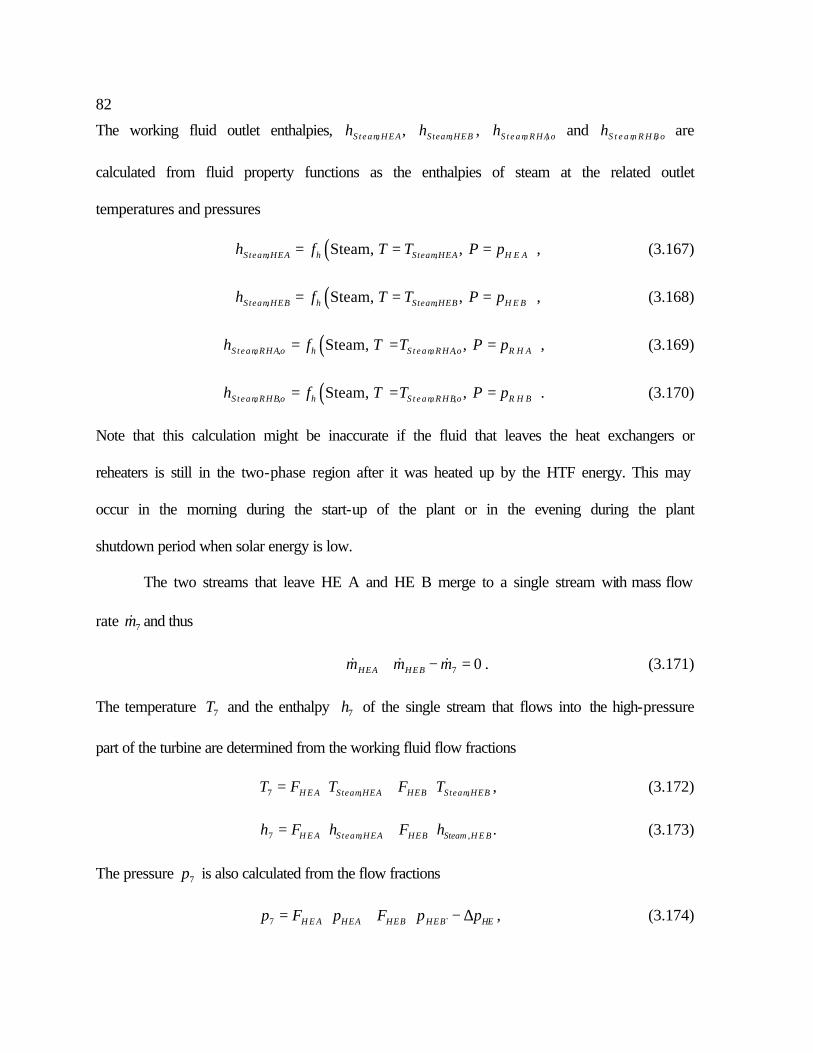
82

The working fluid outlet enthalpies, ,S teamHEAh , ,SteamHEBh , , ,S t e a m R H A oh and , ,S t e a m R H B oh are

calculated from fluid property functions as the enthalpies of steam at the related outlet

temperatures and pressures

( ), ,Steam, ,SteamHEA h SteamHEA H E Ah f T T P p= = = , (3.167)

( ), ,Steam, ,SteamHEB h SteamHEB H E Bh f T T P p= = = , (3.168)

( ), , , ,Steam, ,S teamRHAo h S t e a m R H A o R H Ah f T T P p= = = , (3.169)

( ), , , ,Steam, ,S teamRHBo h S t e a m R H B o R H Bh f T T P p= = = . (3.170)

Note that this calculation might be inaccurate if the fluid that leaves the heat exchangers or

reheaters is still in the two-phase region after it was heated up by the HTF energy. This may

occur in the morning during the start-up of the plant or in the evening during the plant

shutdown period when solar energy is low.

The two streams that leave HE A and HE B merge to a single stream with mass flow

rate 7m& and thus

7 0HEA HEBm m m+ − =& & & . (3.171)

The temperature 7T and the enthalpy 7h of the single stream that flows into the high-pressure

part of the turbine are determined from the working fluid flow fractions

7 , ,H E A SteamHEA HEB SteamHEBT F T F T= ⋅ + ⋅ , (3.172)

7 , ,H E A SteamHEA HEB Steam H E Bh F h F h= ⋅ + ⋅ . (3.173)

The pressure 7p is also calculated from the flow fractions

7 `H E A HEA HEB HEB HEp F p F p p= ⋅ + ⋅ − ∆ , (3.174)

83but from measurements on the real SEGS VI plant, it follows that a pressure drop occurs in

the working fluid on its way from the heat exchanger trains to the high-pressure part of the

turbine. This pressure drop is estimated as a function of the mass flow rate 7m& . The

following polynomial was found from measured data

27 79.81020595 2.7603402 0.278971331HEp m m∆ = − + ⋅ + ⋅& & . (3.175)

The entropy 7s is calculated from fluid property functions as the entropy of steam with the

enthalpy 7h at the pressure 7p

( )7 7 7Steam, ,ss f H h P p= = = . (3.176)

Equations (3.171) – (3.176) form a model for the mixing of the two streams that leave HE A

and HE B. In a similar manner, the mixing of the two streams that leave RH A and RH B can

be described. Thus the following equations are used to calculate the mass flow rate 12m& , the

temperature 12T , the enthalpy 12h , the pressure 12p and the entropy 12s of the fluid that enters

the low-pressure part of the turbine:

12 0R H A R H Bm m m+ − =& & & , (3.177)

12 , , , ,R H A S t e a m R H A o R H B S t e a m R H B oT F T F T= ⋅ + ⋅ , (3.178)

12 , , , ,R H A S t e a m R H A o R H B Steam R H B oh F h F h= ⋅ + ⋅ , (3.179)

12 R H A R H A R H B R H B RHp F p F p p= ⋅ + ⋅ − ∆ , (3.180)

212 12124.845039 5.63854205 0.0510125894RHp m m∆ = − + ⋅ − ⋅& & , (3.181)

( )121212 ,,Steam pPhHfs s === . (3.182)

These equations complete the model for HE A, HE B, RH A and RH B that is given through

equations (3.120) – (3.182).

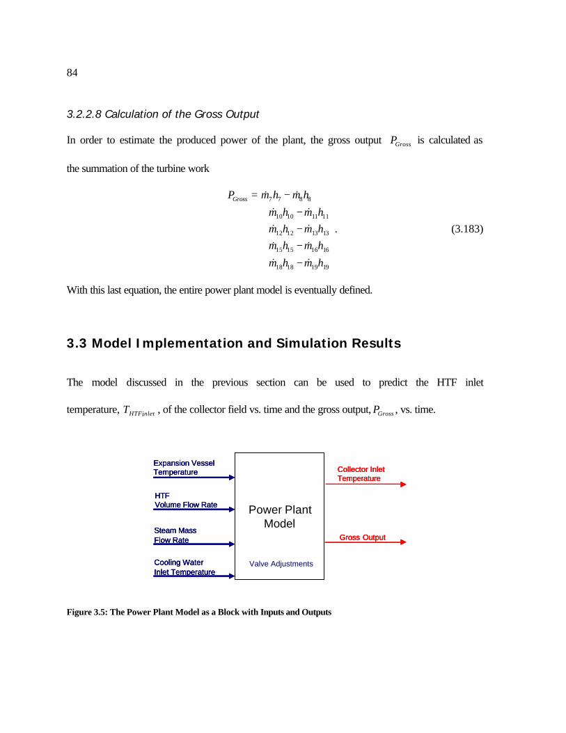
84 3.2.2.8 Calculation of the Gross Output In order to estimate the produced power of the plant, the gross output GrossP is calculated as

the summation of the turbine work

7 7 8 8

10 10 11 11

12 12 13 13

15 15 16 16

18 18 19 19

GrossP m h m h

m h m hm h m hm h m h

m h m h

= −

+ −+ −+ −

+ −

& && && && && &

. (3.183)

With this last equation, the entire power plant model is eventually defined.

3.3 Model Implementation and Simulation Results

The model discussed in the previous section can be used to predict the HTF inlet

temperature, ,HTFinletT , of the collector field vs. time and the gross output, GrossP , vs. time.

Figure 3.5: The Power Plant Model as a Block with Inputs and Outputs

Power PlantModel

Expansion VesselTemperature

HTF Volume Flow Rate

Steam MassFlow Rate

Cooling WaterInlet Temperature

Collector Inlet Temperature

Gross Output

Valve Adjustments

Power PlantModel

Expansion VesselTemperature Expansion VesselTemperature

HTF Volume Flow RateHTF Volume Flow Rate

Steam MassFlow RateSteam MassFlow Rate

Cooling WaterInlet TemperatureCooling WaterInlet Temperature

Collector Inlet TemperatureCollector Inlet Temperature

Gross OutputGross Output

Valve Adjustments

85

The input values of the power plant model are the expansion vessel HTF temperature, ExpT ,

the HTF volume flow rate, HTFV& , the steam mass flow rate, 6m& , and the cooling water inlet

temperature, ,C o o l iT , vs. time. In addition, valve adjustments have to be known that define the

mass flow rates of the turbine extractions. Figure 3.5 shows the power plant model as a block

with inputs and outputs.

Figure 3.6: Measured Expansion Vessel Temperature for September 19, 1998 and for December 14, 1998

Figure 3.7: Measured Steam Mass Flow Rate for September 19, 1998 and for December 14, 1998

5 6 7 8 9 10 11 12 13 14 15 16 17 18 19 20 21 22300

350

400

450

500

550

600

650

700

Time [hr]

T Exp

[K

]

Expansion Vessel Temperature, September 19, 1998

5 6 7 8 9 10 11 12 13 14 15 16 17 18 19 20 21 22300

350

400

450

500

550

600

650

700

Time [hr]

T Exp

[K

]

Expansion Vessel Temperature, December 14, 1998

5 6 7 8 9 10 11 12 13 14 15 16 17 18 19 20 21 220

5

10

15

20

25

30

35

40

Time [hr]

m6 [

kg/s

]

Steam Mass Flow Rate, September 19, 1998

5 6 7 8 9 10 11 12 13 14 15 16 17 18 19 20 21 220

5

10

15

20

25

30

35

40

Time [hr]

m6

[kg

/s]

Steam Mass Flow Rate, December 14, 1998

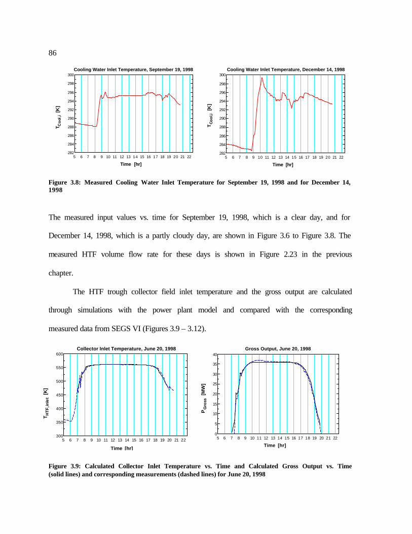
86

Figure 3.8: Measured Cooling Water Inlet Temperature for September 19, 1998 and for December 14, 1998

The measured input values vs. time for September 19, 1998, which is a clear day, and for

December 14, 1998, which is a partly cloudy day, are shown in Figure 3.6 to Figure 3.8. The

measured HTF volume flow rate for these days is shown in Figure 2.23 in the previous

chapter.

The HTF trough collector field inlet temperature and the gross output are calculated

through simulations with the power plant model and compared with the corresponding

measured data from SEGS VI (Figures 3.9 – 3.12).

Figure 3.9: Calculated Collector Inlet Temperature vs. Time and Calculated Gross Output vs. Time (solid lines) and corresponding measurements (dashed lines) for June 20, 1998

5 6 7 8 9 10 11 12 13 14 15 16 17 18 19 20 21 22282

284

286

288

290

292

294

296

298

300

Time [hr]

TC

oo

l,i

[K]

Cooling Water Inlet Temperature, December 14, 1998

5 6 7 8 9 10 11 12 13 14 15 16 17 18 19 20 21 22282

284

286

288

290

292

294

296

298

300

Time [hr]

T Co

ol,i

[K]

Cooling Water Inlet Temperature, September 19, 1998

5 6 7 8 9 10 11 12 13 14 15 16 17 18 19 20 21 22300

350

400

450

500

550

600

Time [hr]

TH

TF

,in

let

[K]

Collector Inlet Temperature, June 20, 1998

5 6 7 8 9 10 11 12 13 14 15 16 17 18 19 20 21 220

5

10

15

20

25

30

35

40

Time [hr]

PG

ross

[M

W]

Gross Output, June 20, 1998

87

Figure 3.10: Calculated Collector Inlet Temperature vs. Time and Calculated Gross Output vs. Time (solid lines) and corresponding measurements (dashed lines) for September 19, 1998

Figure 3.11: Calculated Collector Inlet Temperature vs. Time and Calculated Gross Output vs. Time (solid lines) and corresponding measurements (dashed lines) for December 16, 1998

Figure 3.12: Calculated Collector Inlet Temperature vs. Time and Calculated Gross Output vs. Time (solid lines) and corresponding measurements (dashed lines) for December 14, 1998

5 6 7 8 9 10 11 12 13 14 15 16 17 18 19 20 21 220

5

10

15

20

25

30

35

40

Time [hr]

PG

ros

s [M

W]

Gross Output, September 19, 1998

5 6 7 8 9 10 11 12 13 14 15 16 17 18 19 20 21 22300

350

400

450

500

550

600

Time [hr]

T HT

F,in

let

[K]

Collector Inlet Temperature, September 19, 1998

5 6 7 8 9 10 11 12 13 14 15 16 17 18 19 20 21 22300

350

400

450

500

550

600

Time [hr]

T HT

F,in

let

[K]

Collector Inlet Temperature, December 16, 1998

5 6 7 8 9 10 11 12 13 14 15 16 17 18 19 20 21 220

5

10

15

20

25

30

35

40

Time [hr]

PG

ross

[M

W]

Gross Output, December 16, 1998

5 6 7 8 9 10 11 12 13 14 15 16 17 18 19 20 21 22300

350

400

450

500

550

600

Time [hr]

T HT

F,in

let

[K]

Collector Inlet Temperature, December 14, 1998

5 6 7 8 9 10 11 12 13 14 15 16 17 18 19 20 21 220

5

10

15

20

25

30

35

40

Time [hr]

PG

ros

s [M

W]

Gross Output, December 14, 1998

88Figure 3.9 shows the calculated collector inlet temperature and the calculated gross output vs.

measured data for June 20, 1998. The calculated values, given through the solid line, match

the measured values, represented by the dashed line, sufficiently. The considered day, June

20, 1998, is a day with good weather conditions. For other clear days, September 19, 1998 in

Figure 3.10 and December 16, 1998 in Figure 3.11, the predicted values match the measured

values similarly well.

For a partially cloudy day as December 14, 1998, depicted in Figure 3.12, the

calculated collector inlet temperature and the measured one do not agree as well as for the

clear days. However, the predicted values are still an adequate estimate of the measured

values. The same is true for the calculated gross output.

These results verify that the power plant model as explained above and implemented

in EES is useful as a model for the real SEGS VI power plant. In order to obtain a model for

the entire plant, that is, the trough collector field with the power plant, the trough collector

field model and the power plant model are linked together as explained next.

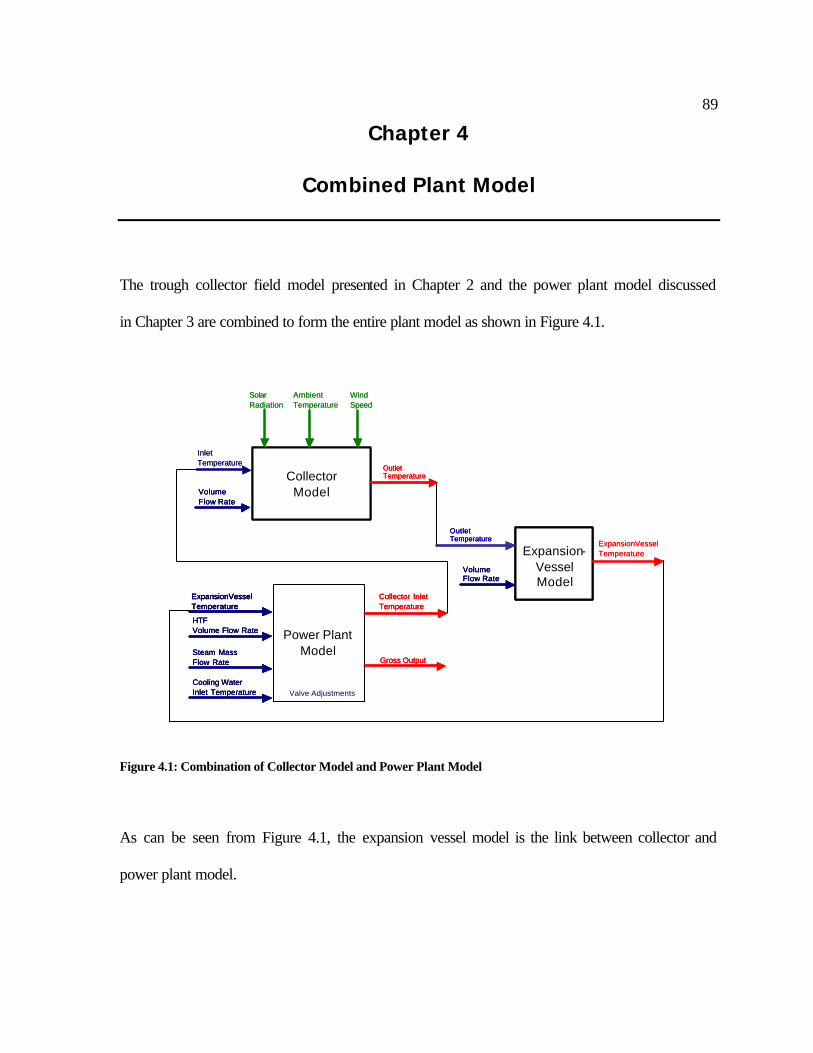
89

Chapter 4

Combined Plant Model

The trough collector field model presented in Chapter 2 and the power plant model discussed

in Chapter 3 are combined to form the entire plant model as shown in Figure 4.1.

Power PlantModel

ExpansionVesselTemperature

HTF Volume Flow Rate

Steam MassFlow Rate

Cooling WaterInlet Temperature

Collector Inlet Temperature

Gross Output

Valve Adjustments

CollectorModel

Inlet Temperature

VolumeFlow Rate

SolarRadiation

AmbientTemperature

WindSpeed

OutletTemperature

Expansion-VesselModel

OutletTemperature

ExpansionVesselTemperature

VolumeFlow Rate

Power PlantModel

ExpansionVesselTemperature

HTF Volume Flow Rate

Steam MassFlow Rate

Cooling WaterInlet Temperature

Collector Inlet Temperature

Gross Output

Valve Adjustments

Power PlantModel

ExpansionVesselTemperatureExpansionVesselTemperature

HTF Volume Flow Rate

Steam MassFlow Rate

Cooling WaterInlet Temperature

Collector Inlet Temperature

Gross Output

Valve Adjustments

CollectorModel

Inlet Temperature

VolumeFlow RateVolumeFlow Rate

SolarRadiation

AmbientTemperature

WindSpeed

OutletTemperatureOutletTemperature

Expansion-VesselModel

Expansion-VesselModel

OutletTemperatureOutletTemperature

ExpansionVesselTemperature

VolumeFlow RateVolumeFlow Rate

Figure 4.1: Combination of Collector Model and Power Plant Model As can be seen from Figure 4.1, the expansion vessel model is the link between collector and

power plant model.

90The expansion vessel is assumed to be a fully mixed tank and thus can be described by a

single differential equation for temperature obtained from an energy balance on the

expansion vessel

0,Exp HTF HTF

Exp HTF jExp Exp

dT V VT T

dt V V= − +

& &. (4.1)

Here, ExpT is the expansion vessel temperature and ExpV is the expansion vessel volume with

3m7.287=ExpV .

The combined plant model can be considered as a single block with inputs and

outputs as depicted in Figure 4.2.

Figure 4.2: The Plant Model as a Block with Inputs and Outputs

Power PlantModel

HTF Volume Flow Rate

Steam MassFlow Rate

Cooling WaterInlet Temperature

Gross Output

Valve Adjustments

CollectorModel

SolarRadiation

AmbientTemperature

WindSpeed

OutletTemperature

Plant Model

Power PlantModel

HTF Volume Flow Rate

Steam MassFlow Rate

Cooling WaterInlet Temperature

Gross OutputGross Output

Valve Adjustments

CollectorModel

SolarRadiation

AmbientTemperature

WindSpeed

OutletTemperature

Plant Model

91

Figure 4.3: With Plant Model calculated Collector Outlet Temperature vs. Time and Gross Output vs. Time (solid lines) and Measured Values (dashed lines) for June 20, 1998

Figure 4.4: With Plant Model calculated Collector Outlet Temperature vs. Time and Gross Output vs. Time (solid lines) and Measured Values (dashed lines) for September 19, 1998

Figure 4.5: With Plant Model calculated Collector Outlet Temperature vs. Time and Gross Output vs. Time (solid lines) and Measured Values (dashed lines) for December 16, 1998

5 6 7 8 9 10 11 12 13 14 15 16 17 18 19 20 21 22300

350

400

450

500

550

600

650

700

Time [hr]

TH

TF

,ou

t [K

]

Collector Outlet Temperature, September 19, 1998

5 6 7 8 9 10 11 12 13 14 15 16 17 18 19 20 21 220

5

10

15

20

25

30

35

40

Time [hr]

PG

ross

[M

W]

Gross Output, September 19, 1998

5 6 7 8 9 10 11 12 13 14 15 16 17 18 19 20 21 22300

350

400

450

500

550

600

650

700

Time [hr]

TH

TF

,ou

t [K

]

Collector Outlet Temperature, December 16, 1998

5 6 7 8 9 10 11 12 13 14 15 16 17 18 19 20 21 220

5

10

15

20

25

30

35

40

Time [hr]

PG

ross

[M

W]

Gross Output, December 16, 1998

5 6 7 8 9 10 11 12 13 14 15 16 17 18 19 20 21 22300

350

400

450

500

550

600

650

700

Time [hr]

TH

TF

,ou

t [K

]Collector Outlet Temperature, June 20, 1998

5 6 7 8 9 10 11 12 13 14 15 16 17 18 19 20 21 220

5

10

15

20

25

30

35

40

Time [hr]

PG

ross

[M

W]

Gross Output, June 20, 1998

92

Figure 4.6: With Plant Model calculated Collector Outlet Temperature vs. Time and Gross Output vs. Time (solid lines) and Measured Values (dashed lines) for December 14, 1998 The combined plant model was implemented in EES and measured data from the real SEGS

VI plant were chosen as inputs. The measured inputs are the HTF volume flow rate (Figure

2.23), the steam mass flow rate (Figure 3.7), the cooling water inlet temperature (Figure 3.8)

and environmental data as the direct normal solar radiation (Figure 2.24), the ambient

temperature (Figure 2.25) and the wind speed (Figure 2.26). The collector outlet temperature

and the gross output as the two considered outputs of the plant, are calculated through

simulations with the plant model and compared with measured data from SEGS VI.

Figure 4.3 shows in the left-hand side figure the plant model calculated collector

outlet temperature vs. the measured collector outlet temperature for June 20, 1998. The

calculated values, given through the solid line, match the measured values, represented by the

dashed line, well. There is also good agreement between the calculated gross output and the

measured gross output. The slight difference between calculated and measured values that

can be seen at around 11 hr is probably due to an inaccurate measurement of the steam mass

5 6 7 8 9 10 11 12 13 14 15 16 17 18 19 20 21 22300

350

400

450

500

550

600

650

700

Time [hr]

TH

TF

,ou

t [K

]

Collector Outlet Temperature, December 14, 1998

5 6 7 8 9 10 11 12 13 14 15 16 17 18 19 20 21 220

5

10

15

20

25

30

35

40

Time [hr]

PG

ross

[M

W]

Gross Output, December 14, 1998

93flow rate at SEGS VI that was used as an input to the plant model for the simulation. June 20,

1998 was a clear day and for the other clear days that are considered, September 19, 1998 in

Figure 4.4 and December 16, 1998 in Figure 4.5, similar good results can be stated.

Even for the partially cloudy day, December 14, 1998, the calculated collector outlet

temperature and the calculated gross output match the measured values well as shown in

Figure 4.6.

These results show that the plant model, as it was described in this and the previous

chapters, is very useful to predict the collector outlet temperature and the produced power of

the real SEGS VI plant. For this model, a control algorithm has to be found that obtains the

ability to hold the collector outlet temperature at a constant set point through the adjustment

of the HTF volume flow rate. The control algorithm that was chosen for this study is taken

from the model predictive control framework as explained in Rawlings and Muske (1993). Its

implementation and performance for the plant model is described in the next chapter.

94

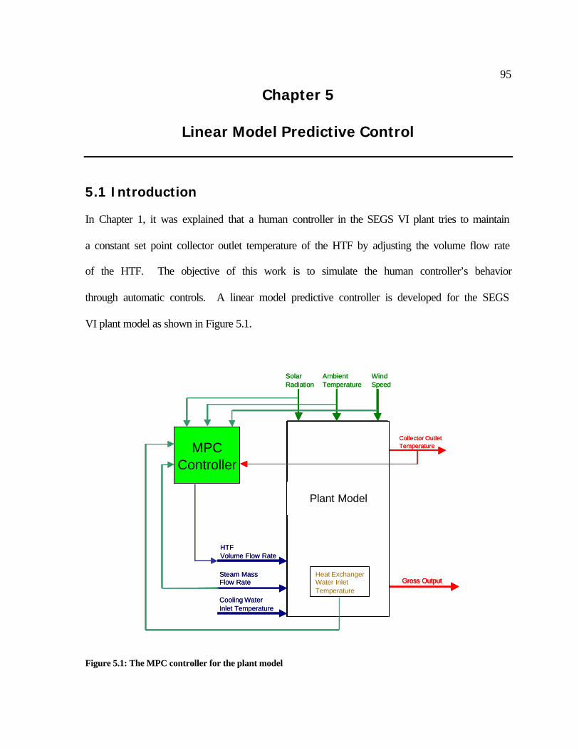
95

Chapter 5

Linear Model Predictive Control

5.1 Introduction In Chapter 1, it was explained that a human controller in the SEGS VI plant tries to maintain

a constant set point collector outlet temperature of the HTF by adjusting the volume flow rate

of the HTF. The objective of this work is to simulate the human controller’s behavior

through automatic controls. A linear model predictive controller is developed for the SEGS

VI plant model as shown in Figure 5.1.

Figure 5.1: The MPC controller for the plant model

Power PlantModel

HTF Volume Flow Rate

Steam MassFlow Rate

Cooling WaterInlet Temperature

Gross Output

Valve Adjustments

CollectorModel

SolarRadiation

AmbientTemperature

WindSpeed

Collector OutletTemperature

Plant Model

MPCController

Heat ExchangerWater InletTemperature

Power PlantModel

HTF Volume Flow Rate

Steam MassFlow Rate

Cooling WaterInlet Temperature

Gross OutputGross Output

Valve Adjustments

CollectorModel

SolarRadiation

AmbientTemperature

WindSpeed

Collector OutletTemperature

Plant Model

MPCController

Heat ExchangerWater InletTemperature

96The MPC controller measures the collector outlet temperature, the solar radiation, the

ambient temperature, the wind speed, the steam mass flow rate in the power plant and the

heat exchanger train water inlet temperature to calculate the HTF volume flow rate that

drives the collector outlet temperature into the set point.

Linear model predictive control (MPC) is a linear optimal control strategy: the

essence of MPC is to optimize, over the manipulable inputs, forecasts of process behavior

(Rawlings, 2000). A feature of MPC is the incorporation of constraints on the manipulated

and controlled variables into the optimization procedure.

In the case of SEGS VI, forecasts of process behavior mean the prediction of how the

collector field outlet temperature of the HTF will behave for a possible variation of the HTF

volume flow rates from now to a point of time in the future. The difference between now and

a future point in time is called the time horizon. If a forecast is made at successive points in

time, there is at each of these points in time a prediction made along a time horizon of the

same length. Thus it is thought of a horizon that moves with time from one prediction point

of time to the next. This is why MPC belongs to a class of control algorithms also referred to

as receding horizon control or moving horizon control.

The optimization of forecasts of process behavior implies that there is a performance

objective. What is the optimal forecasted process behavior? Since an optimization is usually

formulated as a minimization, the performance objective is formulated as a minimization of a

cost functional that is minimal for the optimal forecasted process behavior. The goal of the

human controller at SEGS VI is to maintain the HTF collector field outlet temperature at a

specified set point. Thus, the optimal forecasted process behavior is that the future HTF

collector field outlet temperatures are at the set point and that no change in the HTF volume

97flow rate occure from one point in time to the next point in time. The second criterion reflects

the desire of not having rapid changes in the flow rate. This criterion may be useful for

damping potential oscillations in the HTF collector field outlet temperature while

approaching the set point. Consequently, the value of a cost function that is to be minimized

must increase with an increasing difference between the forecasted HTF collector field outlet

temperatures and the set point temperature. It also must increase with an increasing change in

the HTF volume flow rate from one point in time to the next point in time. The aim is to find

the optimal sequence of HTF volume flow rates among all possible flow rates, that

minimizes the cost function, while keeping the HTF volume flow rates and also the

dependent HTF collector field outlet temperatures between specified upper and lower

bounds. A solution to this problem through MATLAB optimization procedures will be

shown later.

The MPC algorithms presented here are based on a theoretical framework taken from

Rawlings and Muske (1993). In order to obtain a better understanding of the subject, a

simplified model rather than the SEGS VI plant model is chosen to explain the control

strategy. The simplified model is presented next.

5.2 The Simplified Model

The simplified model, shown in Figure 5.2, consists of four elements: a solar collector, an

expansion vessel, a heat exchanger and a HTF pump. Differential equations for temperature

are used to model the system. The simplified system can be described by a system of four

nonlinear differential equations as explained in the following.

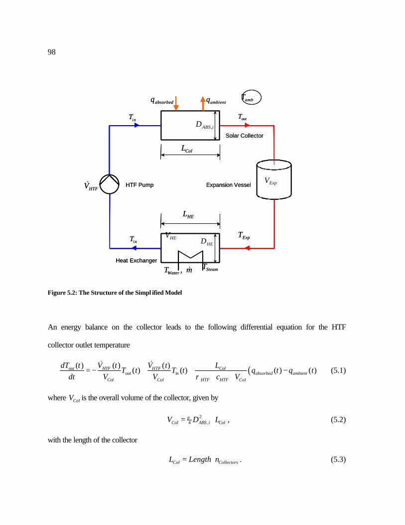
98

Figure 5.2: The Structure of the Simpl ified Model

An energy balance on the collector leads to the following differential equation for the HTF

collector outlet temperature

( )( ) ( ) ( )( ) ( ) ( ) ( )out ColHTF HTF

out in absorbed ambientCol Col HTF HTF Col

dT t LV t V tT t T t q t q t

dt V V c Vρ= − + + −

& & (5.1)

where ColV is the overall volume of the collector, given by

2,4Col ABS i ColV D Lπ= ⋅ , (5.2)

with the length of the collector

Col CollectorsL Length n= ⋅ . (5.3)

HEV

mTWater &,

HEL

iABSD ,

HED

absorbedq ambientq

HTFV&

inT

inT

outT

ambT

HTF Pump

Heat Exchanger

Expansion Vessel

Solar Collector

SteamT

ColL

ExpV

ExpTHEV

mTWater &,

HEL

iABSD ,

HED

absorbedq ambientq

HTFV&

inT

inT

outT

ambT

HTF Pump

Heat Exchanger

Expansion Vessel

Solar Collector

SteamT

ColL

ExpV

ExpT

99

The heat transfer to the environment, ambientq , is described by

( ), ,( ) ( ) ( )ambient ambient ABSsurf i out ambq t h A T t T t= − (5.4)

with a heat transfer coefficient of -1-2KWm5.2=ambienth and the surface area , ,ABS surf iA from

equation (2.22). The initial condition for equation (5.1) is

initoutout TT ,)0( = . (5.5)

The expansion vessel temperature is determined through

( ) ( ) ( )( ) ( )Exp HTF HTF

Exp outExp Exp

dT t V t V tT t T t

dt V V= − +

& & (5.6)

with the expansion vessel volume, 3287.7 mExpV = . The initial condition for equation (5.6)

is

,(0)Exp ExpinitT T= . (5.7)

Finally, the loop is closed through an energy balance on the heat exchanger trains

( ) ( ) ( ) ( ) ( )( ) ( ) ( )in A B HTF A B HTF HE

in Exp transferredHE HE HTF HTF HE

dT t a a V t a a V t LT t T t q t

dt V V c Vρ+ ⋅ + ⋅

= − + −& &

(5.8)

where Aa and Ba are the flow fractions from Chapter 3.2.3.7. The heat transfer in the heat

exchanger is given by

( ),( ) ( ) ( ) ( )transferred HE HEsurf h cq t h t A T t T t= − , (5.9)

where the temperature of the hot fluid, hT , is the mean temperature of the HTF in the heat

exchanger

( )12( ) ( ) ( )h Exp inT t T t T t= + (5.10)

100

and the temperature of the cold working fluid, cT , is the mean temperature

( ))()()( 21 tTtTtT WaterSteamc += . (5.11)

The heat transfer coefficient, HEh , is dependent on the two flow rates that are available as

measurements from SEGS VI

1-2-00, KWm2

/)(/)(74000)(

+⋅=

mtmVtVth HTFHTF

HE

&&&& (5.12)

where m& is the mass flow rate of the working fluid (water or steam). The reference flow rates

are -130, sm624.0=HTFV& for the HTF volume flow rate and -1

0 skg9.39=m& for the mass

flow rate of the working fluid. They are flow rates at solar noon measured at June 20, 1998.

The surface area is determined from

,HE surf HEA Dπ= (5.13)

with an assumed diameter of m1=HED . The volume of the heat exchanger, HEV , is

calculated from

HEHEHE LDV 24π= (5.14)

with an assumed length of m10=HEL . The initial condition for equation (5.8) is

initinin TT ,)0( = . (5.15)

The temperature of the Steam, SteamT , is calculated from a heat exchanger effectiveness

equation

( ) ( )( )

( ) ( )Steam Water

HEExp Water

T t T tt

T t T tε

−=

−, (5.16)

101formulated as the following differential equation

( ) ( )( )( )0.01 ( ) ( ) ( ) ( ) ( )Steam

Steam HE Exp Water Water

dT tT t t T t T t T t

dtε= ⋅ − + − + . (5.17)

The algebraic equation (5.16) is formulated as a differential equation (5.17) because the

model predictive control framework as used in this work considers only differential equations

as system equations. The factor 0.01 s-1 was introduced to adjust the time constant of this

differential equation to the time constant range of the entire system in order to avoid a stiff

differential equation system. The heat exchanger effectiveness is assumed to be flow rate

dependent

025.12

/)(/)()1.0()( 00, +

+⋅−=

mtmVtVt HTFHTF

HE

&&&&ε . (5.18)

The initial condition for equation (5.17) is

initSteamSteam TT ,)0( = . (5.19)

The validation of the simplified model is shown in Figure 5.3 for June 20, 1998, a clear day,

and in Figure 5.4 for December 14, 1998, a partially cloudy day, where the measured input

values for the simplified model are the direct normal solar radiation to calculate absorbedq , the

ambient temperature, ambientT , the HTF volume flow rate, HTFV& , the working fluid mass flow

rate, m& , and the water inlet temperature of the heat exchanger, WaterT . Calculated are the

collector outlet temperature, outT , and the steam outlet temperature of the heat exchanger,

SteamT .

As seen from Figure 5.3 and Figure 5.4, the simplified model can be used to calculate

acceptable HTF temperatures compared to the ones measured at SEGS VI.

102

Figure 5.3: The simplified model calculated collector outlet temperature (solid line) and measured collector outlet temperature (dashed line) are shown in the left hand figure and the calculated steam temperature (solid line) and measured steam temperature (dashed line) are shown in the right hand figure for June 20, 1998

Figure 5.4: The simplified model calculated collector outlet temperature (solid line) and measured collector outlet temperature (dashed line) are shown in the left hand figure and the calculated steam temperature (solid line) and measured steam temperature (dashed line) are shown in the right hand figure for December 14, 1998

In what follows, the simplified model is used to explain the model predictive control scheme.

The name of the control method indicates: a model of the controlled system plays the major

role. It is used to predict values over the time horizon. For the control algorithm presented by

5 6 7 8 9 10 11 12 13 14 15 16 17 18 19 20 21 22300

350

400

450

500

550

600

650

700

Time [hr]

Tou

t [K

]

Collector Outlet Temperature - Simplified Model

5 6 7 8 9 10 11 12 13 14 15 16 17 18 19 20 21 22400

450

500

550

600

650

700

Time [hr]

TS

team

[K

]

Steam Temperature - Simplified Model

5 6 7 8 9 10 11 12 13 14 15 16 17 18 19 20 21 22300

350

400

450

500

550

600

650

700

Time [hr]

Tou

t [K

]

Collector Outlet Temperature - Simplified Model

5 6 7 8 9 10 11 12 13 14 15 16 17 18 19 20 21 22400

450

500

550

600

650

700

Time [hr]

T Ste

am [

K]

Steam Temperature - Simplified Model

103Rawlings and Muske (1993), linear equations are needed. In the next section, it is explained

how the simplified model has to be transformed to obtain linear equations.

5.3 Models for Linear MPC The models in linear MPC are discrete-time linear models in state-space form. First, the

linear model in state-space form is explained, later the time discretization of this model.

The state-space form of a linear model or better linear differential system is

)()()()()( tutBtxtAtx +=& . (5.20)

Here t is the time variable, )(tx is a real n-dimensional time-varying column vector which

denotes the state of the system, and )(tu is a real m-dimensional column vector which

indicates the input variable (Kwakernaak & Sivan, 1972). The time-varying matrix )(tA is of

dimension )( nn × and the time-varying matrix )(tB is of dimension )( mn × . Let )(ty be a

real p-dimensional system variable that can be observed or measured or through which the

system influences its environment.

Such a variable is called an output variable of the system and is expressed through the

output equation of the system

)()()()()( tutDtxtCty += (5.21)

with the time-varying matrix )(tC of dimension )( np × and the time-varying matrix )(tD of

dimension )( mp × . There exists an initial condition for the system described by equation

(5.20)

initxx =)0( . (5.22)

104If the matrices A, B, C, and D are constant, the system is time-invariant:

)()()( tuBtxAtx +=& , (5.23)

)()()( tuDtxCty += . (5.24)

For linear MPC as it is considered in this work, it is necessary to obtain model equations in

the form of equation (5.23) and (5.24) with an initial condition (5.22). Does the simplified

model already obtain this form? If not, what has to be done to gain a system model of that

form?

To answer the first question, the simplified model equations (5.1), (5.6), (5.8) and

(5.17) are written down again with the introduction of some abbreviations. The time constant

Colτ for the collector is defined as

Col

HTF

Col VtV

t)(

)(1 &

=τ

. (5.25)

The crosssectional area of the collector is ColA . An overall heat transfer coefficient-area

product, ColUA , is introduced as

, ,Col ambient ABS surf iUA h A= . (5.26)

With these definitions, the differential equation for the collector outlet temperature (5.1) may

now be written as

( ) ( )( ) ( ))()(

)()()()()(

)(1)(

tTctTAtTtTUAtq

tTtTtdt

tdT

outHTFoutHTFCol

amboutColabsorbedoutin

Col

out

ρτ−−

+−= . (5.27)

There is a time constant for the expansion vessel, Expτ , given through

Exp

HTF

Exp VtV

t)(

)(1 &

=τ

. (5.28)

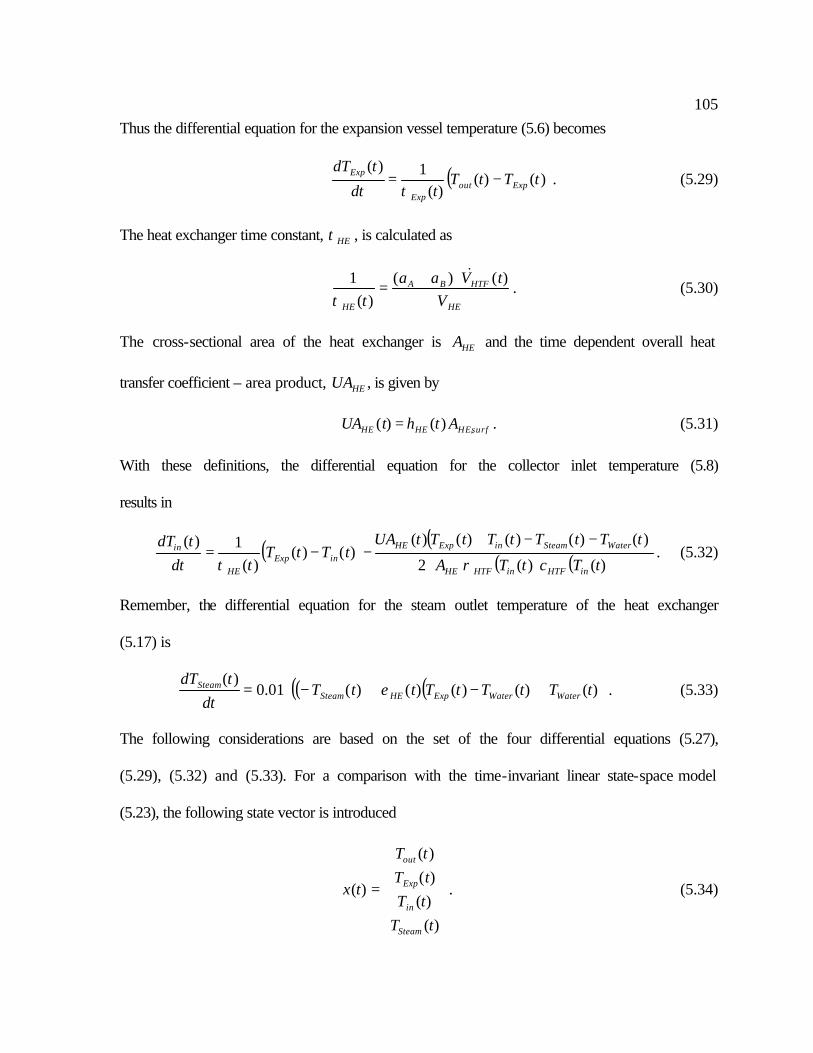
105Thus the differential equation for the expansion vessel temperature (5.6) becomes

( ))()()(

1)(tTtT

tdt

tdTExpout

Exp

Exp −=τ

. (5.29)

The heat exchanger time constant, HEτ , is calculated as

HE

HTFBA

HE VtVaa

t)()(

)(1 &⋅+

=τ

. (5.30)

The cross-sectional area of the heat exchanger is HEA and the time dependent overall heat

transfer coefficient – area product, HEUA , is given by

,( ) ( )HE HE HEsurfUA t h t A= . (5.31)

With these definitions, the differential equation for the collector inlet temperature (5.8)

results in

( ) ( )( ) ( ))()(2

)()()()()()()(

)(1)(

tTctTA

tTtTtTtTtUAtTtT

tdttdT

inHTFinHTFHE

WaterSteaminExpHEinExp

HE

in

ρτ ⋅

−−+−−= . (5.32)

Remember, the differential equation for the steam outlet temperature of the heat exchanger

(5.17) is

( ) ( )( ))()()()()(01.0)(

tTtTtTttTdt

tdTWaterWaterExpHESteam

Steam +−+−⋅= ε . (5.33)

The following considerations are based on the set of the four differential equations (5.27),

(5.29), (5.32) and (5.33). For a comparison with the time-invariant linear state-space model

(5.23), the following state vector is introduced

=

)()()()(

)(

tTtTtTtT

tx

Steam

in

Exp

out

. (5.34)

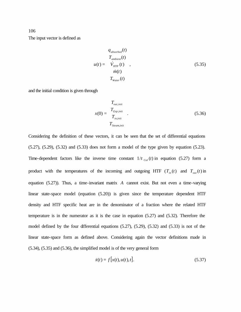
106The input vector is defined as

=

)()(

)()(

)(

)(

tTtm

tVtT

tq

tu

Water

HTF

ambient

absorbed

&& , (5.35)

and the initial condition is given through

=

initSteam

initin

initExp

initout

TTTT

x

,

,

,

,

)0( . (5.36)

Considering the definition of these vectors, it can be seen that the set of differential equations

(5.27), (5.29), (5.32) and (5.33) does not form a model of the type given by equation (5.23).

Time-dependent factors like the inverse time constant )(/1 tColτ in equation (5.27) form a

product with the temperatures of the incoming and outgoing HTF ( )(tTin and )(tTout in

equation (5.27)). Thus, a time-invariant matrix A cannot exist. But not even a time-varying

linear state-space model (equation (5.20)) is given since the temperature dependent HTF

density and HTF specific heat are in the denominator of a fraction where the related HTF

temperature is in the numerator as it is the case in equation (5.27) and (5.32). Therefore the

model defined by the four differential equations (5.27), (5.29), (5.32) and (5.33) is not of the

linear state-space form as defined above. Considering again the vector definitions made in

(5.34), (5.35) and (5.36), the simplified model is of the very general form

[ ]ttutxftx ),(),()( =& . (5.37)

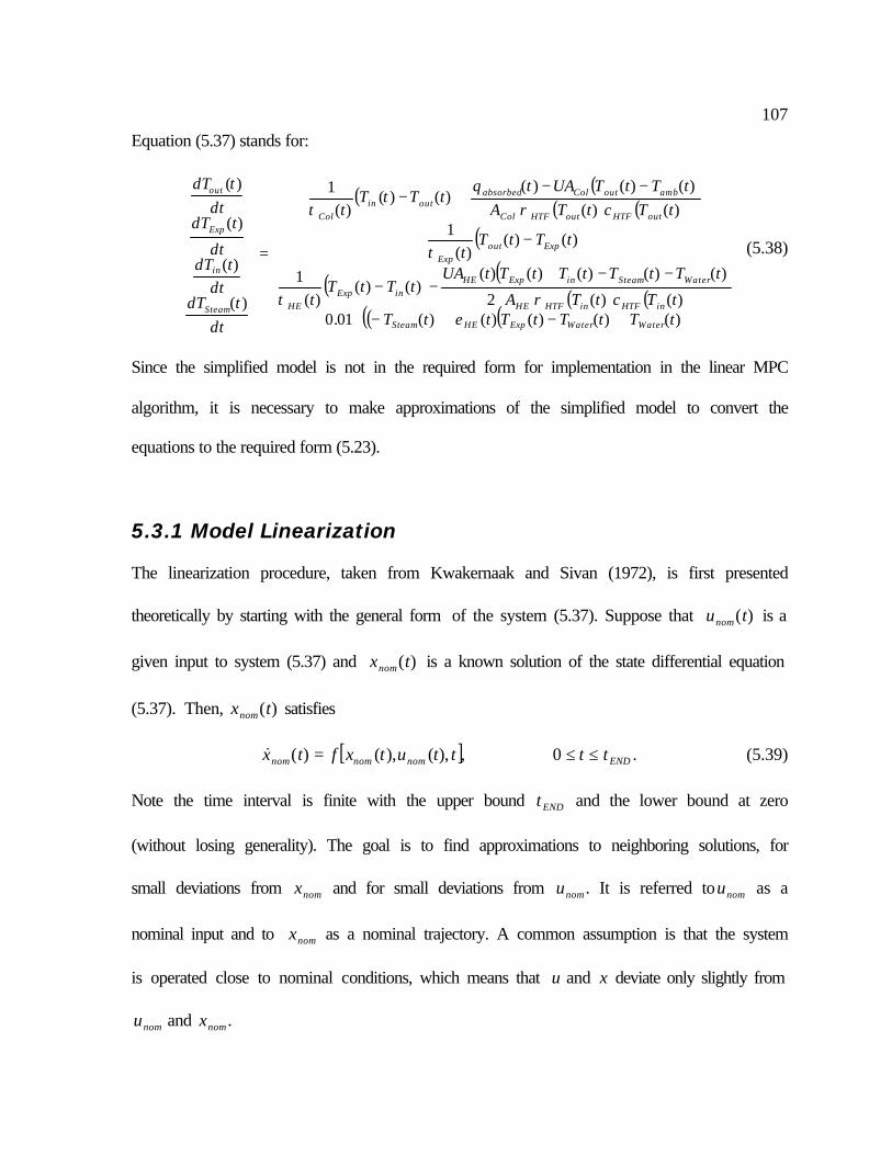
107Equation (5.37) stands for:

( ) ( )( ) ( )

( )

( ) ( )( ) ( )

( ) ( )( )

+−+−⋅⋅

−−+−−

−

−−+−

=

)()()()()(01.0)()(2

)()()()()()()(

)(1

)()()(

1)()(

)()()()()(

)(1

)(

)(

)(

)(

tTtTtTttTtTctTA

tTtTtTtTtUAtTtT

t

tTtTt

tTctTAtTtTUAtq

tTtTt

dttdT

dttdT

dt

tdTdt

tdT

WaterWaterExpHESteam

inHTFinHTFHE

WaterSteaminExpHEinExp

HE

ExpoutExp

outHTFoutHTFCol

amboutColabsorbedoutin

Col

Steam

in

Exp

out

ερτ

τ

ρτ

(5.38)

Since the simplified model is not in the required form for implementation in the linear MPC

algorithm, it is necessary to make approximations of the simplified model to convert the

equations to the required form (5.23).

5.3.1 Model Linearization The linearization procedure, taken from Kwakernaak and Sivan (1972), is first presented

theoretically by starting with the general form of the system (5.37). Suppose that )(tunom is a

given input to system (5.37) and )(txnom is a known solution of the state differential equation

(5.37). Then, )(txnom satisfies

[ ] ENDnomnomnom ttttutxftx ≤≤= 0,),(),()(& . (5.39) Note the time interval is finite with the upper bound ENDt and the lower bound at zero

(without losing generality). The goal is to find approximations to neighboring solutions, for

small deviations from nomx and for small deviations from nomu . It is referred to nomu as a

nominal input and to nomx as a nominal trajectory. A common assumption is that the system

is operated close to nominal conditions, which means that u and x deviate only slightly from

nomu and nomx .

108Thus it can be written

ENDnom tttututu ≤≤+= 0),(~)()( , (5.40)

),0(~)0()0( xxx nom += (5.41)

where )(~ tu and )0(~x are small perturbations. Correspondingly, it is

ENDnom tttxtxtx ≤≤+= 0),(~)()( . (5.42)

After substituting equation (5.40) and equation (5.42) into the state differential equation

(5.37), a Taylor expansion is made, yielding

[ ] [ ][ ] ENDnomnomu

nomnomxnomnomnom

tthottuttutxJtxttutxJttutxftxtx

≤≤+++=+

0,)(~),(),()(~),(),(),(),()(~)( &&

. (5.43)

Here xJ and uJ are the Jacobian matrices of f with respect to x and u. That is, xJ is a

matrix the (i,j)-th element of which is

( ) ,,j

ijix

fJ

ξ∂∂

= (5.44)

where if is the i-th component of f and jξ is the j-th component of x. uJ is similarly defined.

The higher order term, hot, is supposed to be “small” with respect to x~ and u~ and thus is

neglected. Equation (5.43) can then be expressed as

[ ] [ ] ,0),(~),(),()(~),(),()(~ENDnomnomunomnomx tttuttutxJtxttutxJtx ≤≤+=& (5.45)

meaning that x~ and u~ approximately satisfy a linear equation of the form given in equation

(5.20) if [ ]ttutxJtA nomnomx ),(),()( = and [ ]ttutxJtB nomnomu ),(),()( = . Equation (5.45) is

called linearized state differential equation, its initial condition is )0(~x from equation (5.41).

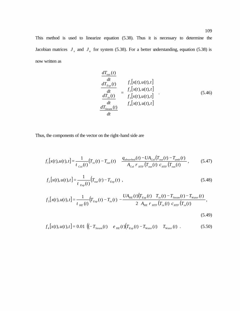
109This method is used to linearize equation (5.38). Thus it is necessary to determine the

Jacobian matrices xJ and uJ for system (5.38). For a better understanding, equation (5.38) is

now written as

[ ][ ][ ][ ]

=

ttutxfttutxfttutxfttutxf

dttdT

dttdT

dt

tdTdt

tdT

Steam

in

Exp

out

),(),(),(),(),(),(),(),(

)(

)(

)(

)(

4

3

2

1

. (5.46)

Thus, the components of the vector on the right-hand side are

[ ] ( ) ( )( ) ( ))()(

)()()()()(

)(1

),(),(1 tTctTAtTtTUAtq

tTtTt

ttutxfoutHTFoutHTFCol

amboutColabsorbedoutin

Col ρτ−−

+−= , (5.47)

[ ] ( ))()()(

1),(),(2 tTtT

tttutxf Expout

Exp

−=τ

, (5.48)

[ ] ( ) ( )( ) ( ))()(2

)()()()()()()(

)(1

),(),(3 tTctTA

tTtTtTtTtUAtTtT

tttutxf

inHTFinHTFHE

WaterSteaminExpHEinExp

HE ρτ ⋅

−−+−−= ,

(5.49)

[ ] ( ) ( )( ))()()()()(01.0),(),(4 tTtTtTttTttutxf WaterWaterExpHESteam +−+−⋅= ε . (5.50)

110From the definition of the Jacobian matrix in equation (5.44) and the state vector in (5.34),

the Jacobian matrix xJ for system (5.38) is

[ ]

∂∂

∂∂

∂∂

∂∂

∂∂

∂∂

∂∂

∂∂

∂∂

∂∂

∂∂

∂∂

∂∂

∂∂

∂∂

∂∂

=

SteaminExpout

SteaminExpout

SteaminExpout

SteaminExpout

x

Tf

Tf

Tf

Tf

Tf

Tf

Tf

Tf

Tf

Tf

Tf

Tf

Tf

Tf

Tf

Tf

ttutxJ

4444

3333

2222

1111

),(),( , (5.51)

and regarding the input vector in (5.35), the Jacobian matrix uJ is

[ ]

∂∂

∂∂

∂∂

∂∂

∂∂

∂∂

∂∂

∂∂

∂∂

∂∂

∂∂

∂∂

∂∂

∂∂

∂∂

∂∂

∂∂

∂∂

∂∂

∂∂

=

WaterHTFambabsorbed

WaterHTFambabsorbed

WaterHTFambabsorbed

WaterHTFambabsorbed

u

Tf

mf

Vf

Tf

qf

Tf

mf

Vf

Tf

qf

Tf

mf

Vf

Tf

qf

Tf

mf

Vf

Tf

qf

ttutxJ

44444

33333

22222

11111

),(),(

&&

&&

&&

&&

. (5.52)

111

In the following, each derivative in the matrices xJ and uJ is listed and new variables for

some of these derivatives are introduced for clarity:

( ) ( )

( ) ( )( )( )

( ) ( )

1

2

1( ) ( ) ( )

( ) ( ) ( )( ) ( )

1( )

( ) ( ) ( )

Col

out Col Col HTF out HTF out

HTF HTFHTF HTF

out outabsorbed Col out amb

Col HTF out HTF out

Col

Col Col HTF out HTF out

UAfT t A T t c T t

cc

T Tq t UA T t T t

A T t c T t

UAN t

t A T t c T t

τ ρ

ρρ

ρ

τ ρ

∂= − −

∂

∂ ∂+ ∂ ∂ − − −

= − − −

, (5.53)

01 =∂∂

ExpTf

, (5.54)

)(11

tTf

Colin τ=

∂∂

, (5.55)

01 =∂

∂

SteamTf

. (5.56)

…………………………………………………………………………………………………..

)(12

tTf

Expout τ=

∂∂

, (5.57)

)(12

tTf

ExpExp τ−=

∂∂

, (5.58)

02 =∂∂

inTf

, (5.59)

02 =∂

∂

SteamTf

. (5.60)

112

03 =∂∂

outTf

, (5.61)

( ) ( ))()(2)(

)(13

tTctTAtUA

tTf

inHTFinHTFHE

HE

HEExp ρτ ⋅−=

∂∂

, (5.62)

( ) ( )

( ) ( )( )( )

( ) ( ))(

)()(2)(

)(1

)()()()()()(2

)(

)()(2)(

)(1

2

3

tNtTctTA

tUAt

tTtTtTtTtTctTA

Tc

cT

tUA

tTctTAtUA

tTf

HEinHTFinHTFHE

HE

HE

WaterSteamExpininHTFinHTFHE

in

HTFHTFHTF

in

HTFHE

inHTFinHTFHE

HE

HEin

+⋅

−−=

−−+⋅

∂

∂+

∂∂

+

⋅−−=

∂∂

ρτ

ρ

ρρ

ρτ

, (5.63)

( ) ( ))()(2)(3

tTctTAtUA

Tf

inHTFinHTFHE

HE

Steam ρ⋅=

∂∂

. (5.64)

…………………………………………………………………………………………………..

04 =∂∂

outTf

, (5.65)

)(01.04 tTf

HEExp

ε⋅=∂∂

, (5.66)

04 =∂∂

inTf

, (5.67)

01.04 −=∂

∂

SteamTf

. (5.68)

…………………………………………………………………………………………………..

( ) ( ))()(11

tTctTAqf

outHTFoutHTFColabsorbed ρ=

∂∂

, (5.69)

( ) ( ) ,)()(

1

tTctTAUA

Tf

outHTFoutHTFCol

Col

amb ρ=

∂∂

(5.70)

113

( ))()(11 tTtT

VVf

outinColHTF

−=∂

∂& , (5.71)

01 =∂∂mf& , (5.72)

01 =∂

∂

WaterTf

. (5.73)

…………………………………………………………………………………………………..

02 =∂

∂

absorbedqf

, (5.74)

02 =∂∂

ambTf

, (5.75)

( ))()(12 tTtT

VVf

ExpoutExpHTF

−=∂

∂& , (5.76)

02 =∂∂mf& , (5.77)

02 =∂

∂

WaterTf

. (5.78)

…………………………………………………………………………………………………..

03 =∂

∂

absorbedqf

, (5.79)

03 =∂∂

ambTf

, (5.80)

114

( )

( ) ( )( )

( )( ) ( ) 0,

0,

,

3

)()(2)(

)()()(

)()()()()()(4

74000

)()()(

HTFinHTFinHTFHEinExp

HE

BA

WaterSteaminExpinHTFinHTFHEHTF

HEsurf

inExpHE

BA

HTF

VtTctTAtK

tTtTV

aa

tTtTtTtTtTctTAV

A

tTtTV

aaV

f

&

&

&

ρ

ρ

⋅−−

+=

−−+⋅

⋅−

−+

=∂

∂

,

(5.81)

( ) ( )( )

( ) ( ) 0

0

,3

)()(2)(

)()()()()()(4

74000

mtTctTAtK

tTtTtTtTtTctTAm

A

mf

inHTFinHTFHE

WaterSteaminExpinHTFinHTFHE

HEsurf

&

&&

ρ

ρ

⋅−=

−−+⋅

⋅−=

∂∂

, (5.82)

( ) ( ))()(2)(3

tTctTAtUA

Tf

inHTFinHTFHE

HE

Water ρ⋅=

∂∂

. (5.83)

………………………………………………………………………………………………

04 =∂

∂

absorbedqf

, (5.84)

04 =∂∂

ambTf

, (5.85)

( ))()(0005.0

0,

4 tTtTVV

fWaterExp

HTFHTF

−−=∂

∂&& , (5.86)

( ))()(0005.0

0

4 tTtTmm

fWaterExp −−=

∂∂

&& , (5.87)

( ))(101.04 tT

fHE

Water

ε−⋅=∂

∂. (5.88)

115

If the Jacobian matrices xJ from equation (5.51) and uJ from equation (5.52) with their

elements given through equations (5.53) – (5.88) are evaluated for a nominal input, )(tunom ,

and a nominal trajectory, )(txnom , then a time-varying linearized state differential equation of

the form given in equation (5.45) is found. Next, the four linear differential equations are

presented that are found after multiplying and simplifying the right-hand side of equation

(5.45). For a small perturbation of the collector outlet temperature, )(~

tTout , around a nominal

solution, the approximate linear differential equation is

( ) ( ) ( ) ( )

( )

, , , ,

,

, ,

( ) ( )( ) ( )( ) ( ) ( ) ( )

1( ) ( ) ( ) ( )

( )

1( ) ( )

Col out ambout absorbed

Col HTF outnom HTF out nom Col HTF out nom HTF o u t nom

in out nom outColnom

innom out nomCol

UA T t T tdT t q tdt A T t c T t A T t c T t

T t T t N t T tt

T t T t VV

ρ ρ

τ

− = −

+ − +

+ −

% %% %

% % %

&% ( )HTF t

,

(5.89)

with the initial condition

initoutout TT ,~

)0(~

= . (5.90)

The linear differential equation for a small perturbation of the expansion vessel temperature,

ExpT~

, around a nominal solution is

[ ] ( ) )(~

)()(1

)(~

)(~

)(1)(

~

,,,

tVtTtTV

tTtTtdt

tTdHTFnomExpnomout

ExpExpout

nomExp

Exp &−+−=τ

, (5.91)

with the initial condition

initExpExp TT ,~

)0(~

= . (5.92)

116For the collector inlet temperature, the linearized differential equation is

[ ]( )

( ) ( )( )

( ) ( )

+

⋅−

−+

+

+⋅

−−+−

−=

00,,,

,,

,,,

,

,

~)(~

)()(2)(

)(~

)()()(

)(~

)()()(2

)(~

)(~

)(~

)(~

)(

)(~)(~)(

1)(~

mm

VtV

tTctTAtK

tVtTtTV

aa

tTtNtTctTA

tTtTtTtTtUA

tTtTtdt

tTd

HTF

HTF

nominHTFnominHTFHE

nom

HTFnominnomExpHE

BA

innomHEnominHTFnominHTFHE

WaterSteaminExpnomHE

inExpnomHE

in

&&

&&

&

ρ

ρ

τ

, (5.93)

with the initial condition

initinin TT ,~

)0(~

= . (5.94)

Finally, the linear differential equation for a small perturbation of the steam outlet

temperature of the heat exchanger, SteamT~

, around a nominal solution is

( ) ( )[ ]

( )

+−⋅−

+−+−⋅=

00,,,

,

)(~)(~)()(0005.0

)(~

)(~

)(~

)()(~

01.0~

mtm

VtV

tTtT

tTtTtTttTdt

Td

HTF

HTFnomWaternomExp

WaterWaterExpnomHESteamSteam

&&

&&

ε

, (5.95)

with the initial condition

initSteamSteam TT ,~

)0(~

= . (5.96)

To obtain a time-invariant linearized state differential equation from (5.45), a steady-state

situation as nominal solution is considered, where all quantities are constant. A constant

input to the system means that the absorbed solar energy, the ambient temperature, the HTF

volume flow rate, the mass flow rate and the water temperature are held constant. For such a

constant input, temperatures will evolve throughout the plant that stay constant with ongoing

117time if no further change in the input variables occurs. The constant input together with the

constant temperatures is called a steady-state situation. If the constant input is taken as

nominal input, nomu , and the evolved constant temperatures as nominal trajectory, nomx , then

the Jacobian matrices xJ and uJ have constant elements if evaluated for this nominal

solution. In this case, the linearized state differential equation (5.45) is time-invariant and a

model of the form (5.23) is found that can be applied to the MPC algorithm

)(~)(~)(~ tuBtxAtx +=& . (5.97)

However, a slight variation of equation (5.97) is used here since a distinction is made

between manipulable inputs and inputs that cannot be manipulated or that are not considered

to be manipulated for the purpose of the collector outlet temperature control (as the steam

mass flow rate )(tm& in this study). In order to control the collector outlet temperature, only

the HTF volume flow rate )(tVHTF& is adjusted and the following scalar is defined

)()( tVtu HTFm&= . (5.98)

The input variable )(tum stands for manipulable input.

In addition, the vector of non-manipulated inputs is defined as

=

)()(

)()(

)(

tTtm

tTtq

tu

Water

ambient

absorbed

d & . (5.99)

Instead of using the input vector )(tu from equation (5.35), the two input variables )(tum

and )(tud are taken.

118

Thus, the time-invariant matrix B is divided into the vector mB and into the matrix dB to

express equation (5.97) as

)(~)(~)(~)(~ tuBtuBtxAtx ddmm ++=& . (5.100)

The measured output variable )(ty of the system is the collector outlet temperature )(tTout ,

the variable that has to be controlled. From equation (5.24) it follows then

)(~)(~ txCty = , (5.101)

with

[ ]0001=C (5.102)

from the definition of )(tx in equation (5.34).

The linear model given through equations (5.100) and (5.101) with the initial

condition in equation (5.41) is compared to the nonlinear model from equation (5.38). Both

models were implemented in EES to predict the collector outlet temperature )(tTout and the

steam temperature )(tTSteam for a clear day, June 20, 1998 and a partially cloudy day,

December 14, 1998.

Figure 5.5: A comparison between the simplified nonlinear model (solid line) and its linearized model (dashed line) through the prediction of the collector outlet temperature and the steam temperature for June 20, 1998

5 6 7 8 9 10 11 12 13 14 15 16 17 18 19 20 21 22300

350

400

450

500

550

600

650

700

Time [hr]

To

ut [

K]

Nonlinear vs. Linear Model - Collector Outlet Temperature

5 6 7 8 9 10 11 12 13 14 15 16 17 18 19 20 21 22400

450

500

550

600

650

700

Time [hr]

TS

team

[K

]

Nonlinear vs. Linear Model - Steam Temperature

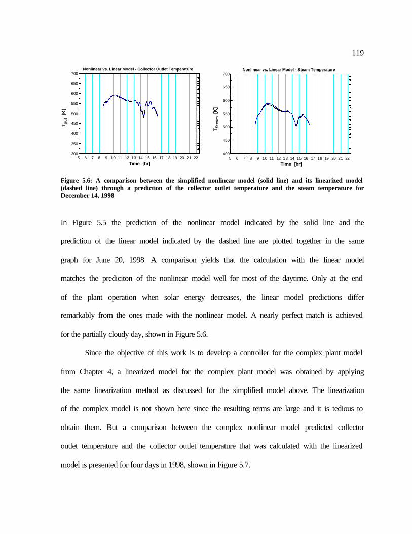
119

Figure 5.6: A comparison between the simplified nonlinear model (solid line) and its linearized model (dashed line) through a prediction of the collector outlet temperature and the steam temperature for December 14, 1998

In Figure 5.5 the prediction of the nonlinear model indicated by the solid line and the

prediction of the linear model indicated by the dashed line are plotted together in the same

graph for June 20, 1998. A comparison yields that the calculation with the linear model

matches the prediciton of the nonlinear model well for most of the daytime. Only at the end

of the plant operation when solar energy decreases, the linear model predictions differ

remarkably from the ones made with the nonlinear model. A nearly perfect match is achieved

for the partially cloudy day, shown in Figure 5.6.

Since the objective of this work is to develop a controller for the complex plant model

from Chapter 4, a linearized model for the complex plant model was obtained by applying

the same linearization method as discussed for the simplified model above. The linearization

of the complex model is not shown here since the resulting terms are large and it is tedious to

obtain them. But a comparison between the complex nonlinear model predicted collector

outlet temperature and the collector outlet temperature that was calculated with the linearized

model is presented for four days in 1998, shown in Figure 5.7.

5 6 7 8 9 10 11 12 13 14 15 16 17 18 19 20 21 22300

350

400

450

500

550

600

650

700

Time [hr]

To

ut

[K]

Nonlinear vs. Linear Model - Collector Outlet Temperature

5 6 7 8 9 10 11 12 13 14 15 16 17 18 19 20 21 22400

450

500

550

600

650

700

Time [hr]

TS

tea

m [

K]

Nonlinear vs. Linear Model - Steam Temperature

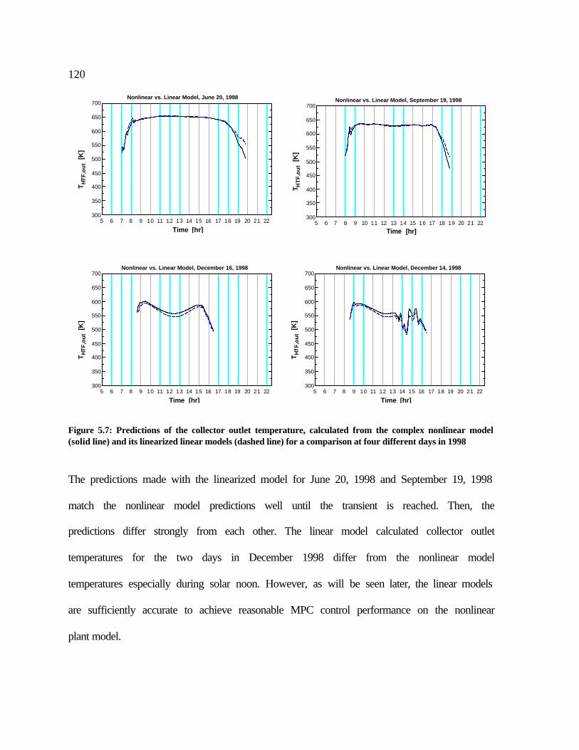
120

Figure 5.7: Predictions of the collector outlet temperature, calculated from the complex nonlinear model (solid line) and its linearized linear models (dashed line) for a comparison at four different days in 1998

The predictions made with the linearized model for June 20, 1998 and September 19, 1998

match the nonlinear model predictions well until the transient is reached. Then, the

predictions differ strongly from each other. The linear model calculated collector outlet

temperatures for the two days in December 1998 differ from the nonlinear model

temperatures especially during solar noon. However, as will be seen later, the linear models

are sufficiently accurate to achieve reasonable MPC control performance on the nonlinear

plant model.

5 6 7 8 9 10 11 12 13 14 15 16 17 18 19 20 21 22300

350

400

450

500

550

600

650

700

Time [hr]

TH

TF

,ou

t [K

]

Nonlinear vs. Linear Model, June 20, 1998

5 6 7 8 9 10 11 12 13 14 15 16 17 18 19 20 21 22300

350

400

450

500

550

600

650

700

Time [hr]

T HT

F,o

ut

[K]

Nonlinear vs. Linear Model, September 19, 1998

5 6 7 8 9 10 11 12 13 14 15 16 17 18 19 20 21 22300

350

400

450

500

550

600

650

700

Time [hr]

TH

TF

,ou

t [K

]

Nonlinear vs. Linear Model, December 16, 1998

5 6 7 8 9 10 11 12 13 14 15 16 17 18 19 20 21 22300

350

400

450

500

550

600

650

700

Time [hr]

TH

TF

,ou

t [K

]

Nonlinear vs. Linear Model, December 14, 1998

121 5.3.2 Discrete-Time Models The linear differential equation system (5.100), the output equation (5.101) and the initial

condition in equation (5.41) form a continuous-time system. However, MPC deals with

discrete-time systems. Consequently, the linear time-invariant continuous-time system has to

be transformed into an equivalent discrete-time system of the form

kdddkmdmkdk uBuBxAx ,,,,1~~~~ ++=+ , (5.103)

kdk xCy ~~ = (5.104)

where kx~ is the state and kmu ,~ , kdu ,

~ the inputs at time instants ,...2,1,0, =ktk The initial

condition is 0~x . The sampling period, ∆ , is the constant difference between two time instants

ii tt −=∆ +1 . (5.105)

A derivation of the following transformation for the discrete-time system can be found in

Kwakernaak and Sivan (1972) and yields

∆= AdA e , (5.106)

1, ( )m d d mB A I A B−= − , (5.107)

1, ( )d d d dB A I A B−= − , (5.108)

CCd = . (5.109)

Through these equations, the discrete-time equations that represent the continuous-time

system are obtained. In the following only the discrete-time system is considered and the d-

index at the matrices is omitted, bearing in mind that the system matrices are the matrices of

a discrete-time system.

122Before the linear discrete-time model is used in the MPC algorithms, equation (5.103) is

augmented by the input step disturbance kd . This results in

( )1 , ,k k m m k k d d kx A x B u d B u+ = + + +% % % % . (5.110)

The affine term kd serves the purpose of adding integral control, what is explained later.

Constraints on the collector outlet temperature as the output and on the HTF volume

flow rate as the manipulable input are considered

, , ,outmin o u t k outmaxT T T≤ ≤% % % , (5.111)

, , ,HTF min HTF k HTF maxV V V≤ ≤& & &% % % , (5.112)

or equivalently

min k maxy y y≤ ≤% % % , (5.113)

, , ,mmin m k mmaxu u u≤ ≤% % % . (5.114)

The time-invariant linear discrete-time model given through (5.110) and (5.104) together

with the constraints (5.113) and (5.114) is now ready for use in the MPC framework from

Rawlings and Muske (1993) that is explained next.

5.4 The Model Predictive Control Framework 5.4.1 Receding Horizon Regulator Formulation As explained in the introduction Chapter 5.1, a cost function that is to be minimized for

optimal control must increase with an increasing difference between the forecasted HTF

collector field outlet temperatures and the set point temperature. In addition, it must increase

with an increasing rate of change in the HTF volume flow rate. Thus the receding horizon

123regulator is based on the minimization of the following infinite horizon open-loop quadratic

objective function at time k (Rawlings & Muske, 1993):

( )2 2, , ,

0

12k o u t k j outset HTF k j

j

Q T T S V∞

+ +=

Φ = − + ∆ ∑ &% % % , (5.115)

where Q is a penalty parameter on the difference between the collector outlet temperature

and the set point temperature with 0Q > . The parameter S with 0S > is a penalty

parameter on the rate of change of the HTF volume flow rate as the input in which

, , , 1HTFk j HTF k j HTF k jV V V+ + + −∆ = −& & &% % % . (5.116)

For this input velocity, the following constraints are considered

max,,min,~~~

HTFkHTFHTF VVV &&& ≤∆≤∆ . (5.117)

The parameters Q and S are the tuning parameters of the receding horizon regulator. A

large value of Q in comparison to S may drive the collector outlet temperature quickly to its

set point at the expense of large changes in the HTF volume flow rate. If S is chosen large

relatively to Q the control action is reduced but the rate at which the collector outlet

temperature approaches its set point is slowed down. Tuning the parameters is a non-trivial

problem in MPC. The cost function in equation (5.115) is now written as

( )2 2,

0

12k k j set m k j

j

Q y y S u∞

+ +=

Φ = − + ∆ ∑ % % % . (5.118)

This follows from equation (5.98) and equation (5.101).

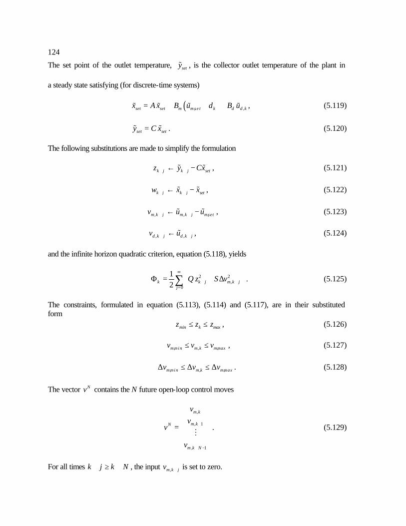
124

The set point of the outlet temperature, sety% , is the collector outlet temperature of the plant in

a steady state satisfying (for discrete-time systems)

( ), ,set set m m s e t k d d kx A x B u d B u= + + +% % % % , (5.119)

set sety C x=% % . (5.120)

The following substitutions are made to simplify the formulation

k j k j setz y Cx+ +← −% % , (5.121)

k j k j setw x x+ +← −% % , (5.122)

, , ,m k j m k j msetv u u+ +← −% % , (5.123)

, ,d k j d k jv u+ +← % , (5.124)

and the infinite horizon quadratic criterion, equation (5.118), yields

2 2,

0

12k k j m k j

j

Q z S v∞

+ +=

Φ = + ∆ ∑ . (5.125)

The constraints, formulated in equation (5.113), (5.114) and (5.117), are in their substituted form

min k maxz z z≤ ≤ , (5.126)

, , ,mmin m k mmaxv v v≤ ≤ , (5.127)

, , ,mmin m k mmaxv v v∆ ≤ ∆ ≤ ∆ . (5.128)

The vector Nv contains the N future open-loop control moves

,

, 1

, 1

m k

m kN

m k N

vv

v

v

+

+ −

=

M . (5.129)

For all times k j k N+ ≥ + , the input ,m k jv + is set to zero.

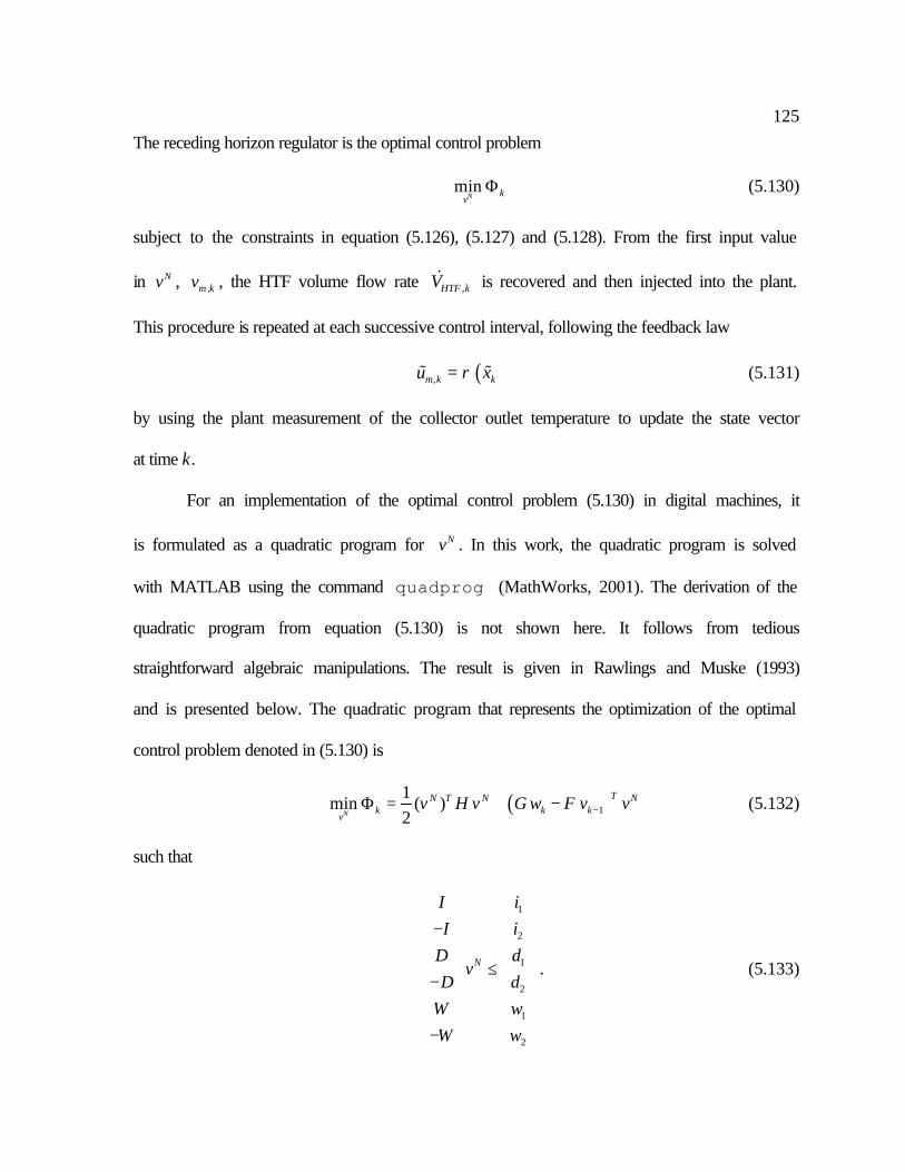
125The receding horizon regulator is the optimal control problem

minN k

vΦ (5.130)

subject to the constraints in equation (5.126), (5.127) and (5.128). From the first input value

in Nv , ,m kv , the HTF volume flow rate ,HTF kV& is recovered and then injected into the plant.

This procedure is repeated at each successive control interval, following the feedback law

( ),m k ku xρ=% % (5.131)

by using the plant measurement of the collector outlet temperature to update the state vector

at time k.

For an implementation of the optimal control problem (5.130) in digital machines, it

is formulated as a quadratic program for Nv . In this work, the quadratic program is solved

with MATLAB using the command quadprog (MathWorks, 2001). The derivation of the

quadratic program from equation (5.130) is not shown here. It follows from tedious

straightforward algebraic manipulations. The result is given in Rawlings and Muske (1993)

and is presented below. The quadratic program that represents the optimization of the optimal

control problem denoted in (5.130) is

( )1

1min ( )

2N

TN T N Nk k k

vv H v G w F v v−Φ = + − (5.132)

such that

1

2

1

2

1

2

N

iIiIdD

vdDwWwW

−

≤ −

−

. (5.133)

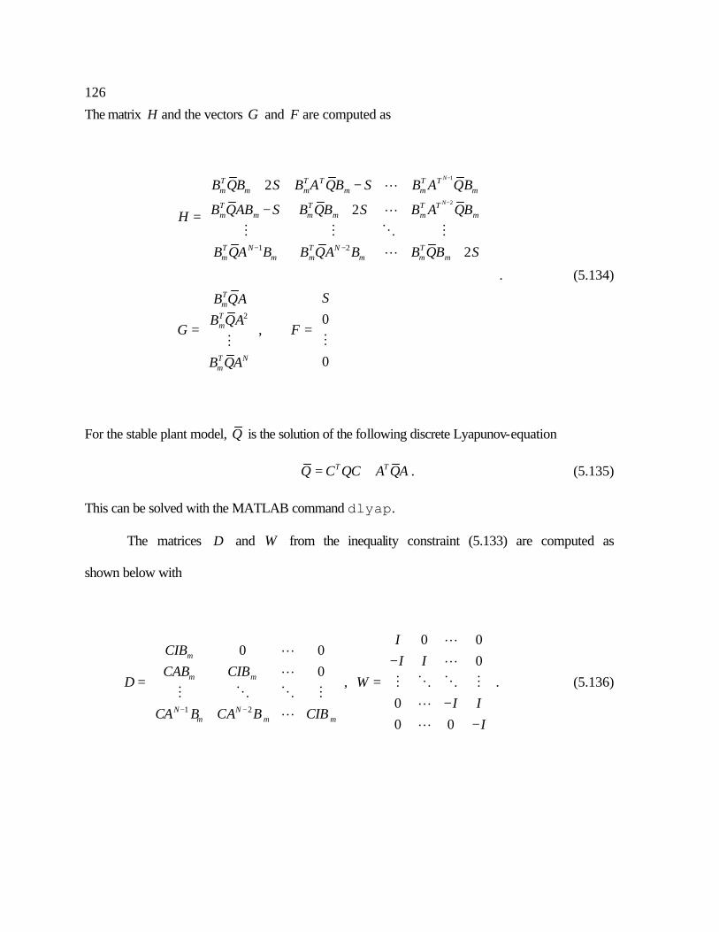
126

The matrix H and the vectors G and F are computed as

1

2

1 2

2

2

2

2

0,

0

N

N

T T T T Tm m m m m m

T T T Tm m m m m m

T N T N Tm m m m m m

Tm

Tm

T Nm

B QB S B A QB S B A QB

B QAB S B QB S B A QBH

B QA B B QA B B QB S

SB QAB QA

G F

B QA

−

−

− −

+ − − += +

= =

LL

M M O ML

MM

. (5.134)

For the stable plant model, Q is the solution of the following discrete Lyapunov-equation

T TQ C QC A QA= + . (5.135)

This can be solved with the MATLAB command dlyap.

The matrices D and W from the inequality constraint (5.133) are computed as

shown below with

1 2

0 00 0

00

,00 0

m

m m

N Nm m m

ICIB

I ICAB CIB

D WI I

CA B CA B CIBI

− −

− = = − −

LL LL M O O MM O O M LL L

. (5.136)

127 The values of the right-hand side vectors in equation (5.133) are the following:

, ,

1 2

, ,

1 2

, , 1 , , 1

, ,1 2

,

, ,

, ,

,

mmax mmin

mmax mmin

max k min k

N Nmax k min k

mmax m k mmin m k

m m a x mmin

mmax

v v

i iv v

z CAw z CAwd d

z CA w z CA w

v v v vv v

w w

v v

− −

− = = −

− − + = = − − +

∆ + ∆ − ∆ ∆ = = ∆ ∆

M M

M M

M M,

.

mmin

(5.137)

The following restrictions are imposed on the constraints to ensure consistence and feasibility

of the origin

,

,

,

,

000000

mmax

mmin

max

min

mmax

mmin

vvzz

vv

−

> − ∆ ∆

. (5.138)

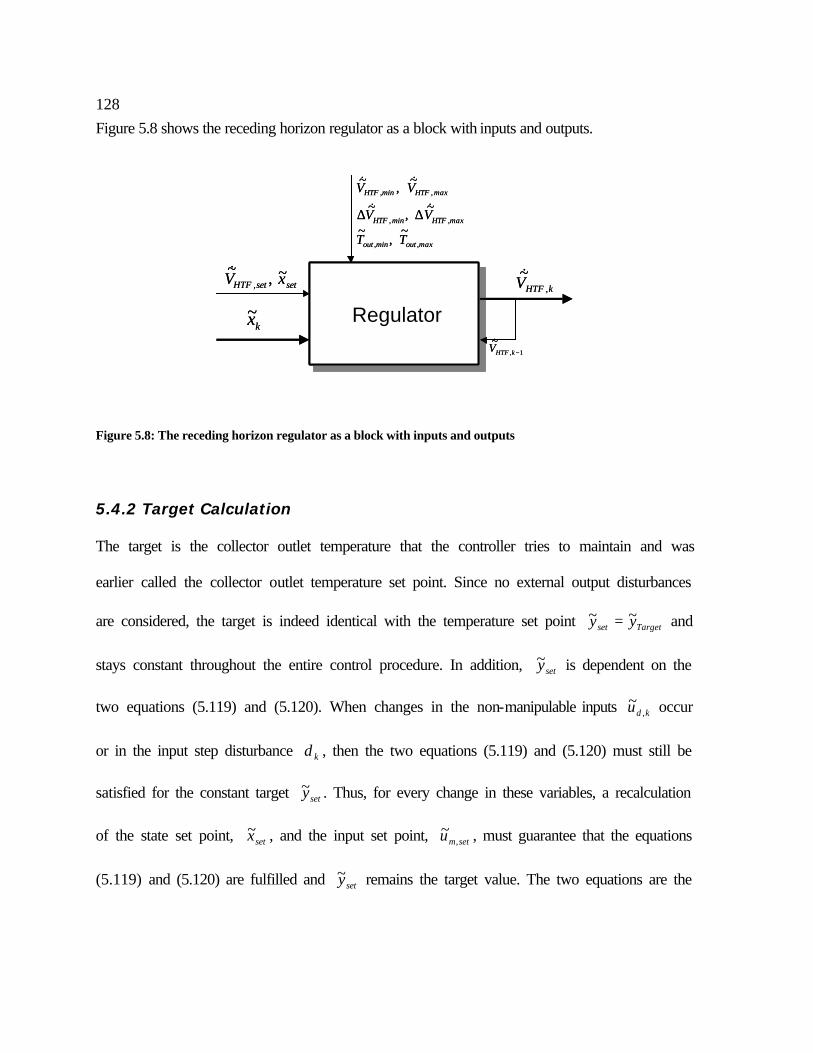
128Figure 5.8 shows the receding horizon regulator as a block with inputs and outputs.

Regulator

maxoutminout

maxHTFminHTF

maxHTFminHTF

TT

VV

VV

,,

,,

,,

~,

~

~,~

~,~

&&&&

∆∆

setsetHTF xV ~,~

,&

kx~kHTFV ,

~&

1,~

−kHTFV&Regulator

maxoutminout

maxHTFminHTF

maxHTFminHTF

TT

VV

VV

,,

,,

,,

~,

~

~,~

~,~

&&&&

∆∆

setsetHTF xV ~,~

,&

kx~kHTFV ,

~&

1,~

−kHTFV&

Figure 5.8: The receding horizon regulator as a block with inputs and outputs 5.4.2 Target Calculation

The target is the collector outlet temperature that the controller tries to maintain and was

earlier called the collector outlet temperature set point. Since no external output disturbances

are considered, the target is indeed identical with the temperature set point Targetset yy ~~ = and

stays constant throughout the entire control procedure. In addition, sety~ is dependent on the

two equations (5.119) and (5.120). When changes in the non-manipulable inputs kdu ,~ occur

or in the input step disturbance kd , then the two equations (5.119) and (5.120) must still be

satisfied for the constant target sety~ . Thus, for every change in these variables, a recalculation

of the state set point, setx~ , and the input set point, setmu ,~ , must guarantee that the equations

(5.119) and (5.120) are fulfilled and sety~ remains the target value. The two equations are the

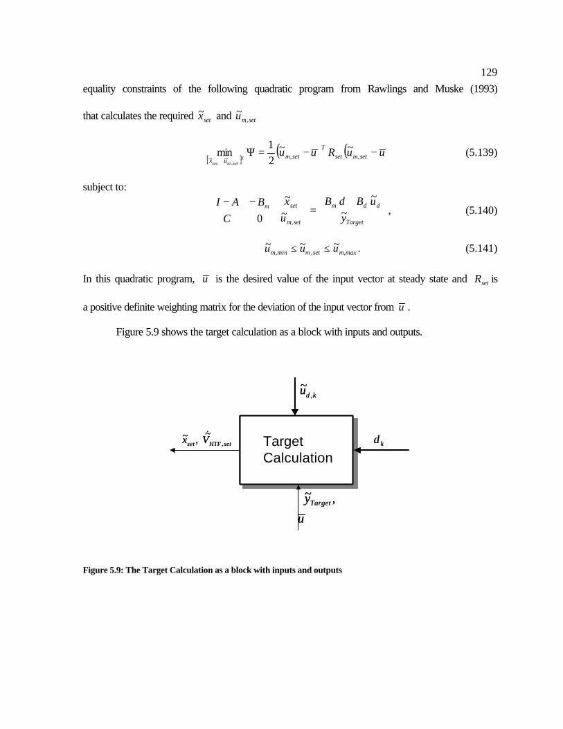
129equality constraints of the following quadratic program from Rawlings and Muske (1993)

that calculates the required setx~ and setmu ,~

[ ]( ) ( )uuRuu setmset

Tsetm

ux Tsetmset

−−=Ψ ,,~~~~

21

min,

(5.139)

subject to:

+=

−−

Target

ddm

setm

setm

yuBdB

ux

CBAI

~~

~~

0 ,

, (5.140)

m,maxsetmm,min uuu ~~~, ≤≤ . (5.141)

In this quadratic program, u is the desired value of the input vector at steady state and setR is

a positive definite weighting matrix for the deviation of the input vector from u .

Figure 5.9 shows the target calculation as a block with inputs and outputs.

TargetCalculation

kd

kdu ,~

,~Targety

u

setHTFset Vx ,~,~ & Target

Calculationkd

kdu ,~

,~Targety

u

setHTFset Vx ,~,~ &

Figure 5.9: The Target Calculation as a block with inputs and outputs

130

5.4.3 State Estimator In the section about the regulator, it was assumed that the states kx~ are measured. In fact,

from the states only the collector outlet temperature koutT , is measured. Thus a method is

sought to estimate the entire state kx~ from the known collector outlet temperature. In

addition to the collector outlet temperature, both the manipulable and the non-manipulable

inputs are known or measured. From these given information, the states are estimated

through an optimal linear observer, called discrete Kalman filter, constructed for the system

( ) ,...2,1,0,~~~~,,1 =++++=+ kGuBduBxAx kkddkkmmkk ξξ (5.142)

kkk dd ω+=+1 (5.143)

kkk xCy ν+= ~~ . (5.144)

In this representation, kξ , kω and kν are zero-mean, uncorrelated, normally distributed,

stochastic variables with covariance matrices ξQ , ωQ and νR respectively.

It was already mentioned that the input step disturbance kd is used for integral

action: in order to obtain offset-free control, it is assumed that the difference between the

Kalman-filter-predicted output and the measured output is caused by an input step

disturbance kd . The input step disturbance can be estimated by the Kalman filter as well if it

is treated as an additional state of the system, accounted by equation (5.143). The estimated

input step disturbance is then used in the target calculation to compensate the offset.

131The system can be rewritten with the following augmented matrices

[ ] 0, , , 0 ,

0 1 0 0 0 1m m d

m d

A B B B GA B B C C G ξ

ξ

= = = = =

% % %% % (5.145)

thus

+++

=

+

+

k

kkddkmm

k

k

k

k GuBuBdx

Adx

ωξ

ξ

~~~~~~~~,,

1

1 , (5.146)

kk

kk d

xCy ν+

=

~~~ . (5.147)

A full-order linear observer for the augmented system (5.146) and (5.147) is

−+++

=

−

−−−

−

−

+

+

1|

1|1|,1|,

1|

1|

|1

|1

ˆˆ~~~~~~

ˆˆ~

ˆˆ

kk

kkkkkddkkmm

kk

kk

kk

kk

dx

CyLuBuBdx

Adx

, (5.148)

where kkx |1ˆ + and kkd |1ˆ

+ is the estimate of the states for time 1+k given output and input

measurements up to time k . The difference between the measured collector outlet

temperature ky~ and the reconstructed output is multiplied by the observer gain L and fed

back to minimize the estimation error, that is, the difference between the real states and the

estimated ones. The stability and the asymptotic behavior of the estimation error are

determined by the choice of L . The observer gain L that minimizes the mean square

estimation error was first solved by Kalman and Bucy and is computed from the solution of

the following discrete filterting steady-state Riccati equation

( )[ ] TTTT GQGAPCRCPCCPPAP ξξξν

~~~~~~~~~ 1++−=

−, (5.149)

( ) 1~~~~ −+= νRCPCCPAL TT . (5.150)

132Here, the following augmented covariance matrix is used

=

ω

ξξ Q

QQ

00~

. (5.151)

The derivation of equation (5.149) and (5.150) is not shown here, it can be found in

Kwakernaak & Sivan (1972). Discrete steady-state Riccati equations can be solved with

MATLAB using the command dare.

Figure 5.10 shows the estimator as a block with inputs and outputs

EstimatorkHTFV ,

~&koutT ,

~

kdu ,~

kkx |1ˆ + kkd |1ˆ

+

EstimatorkHTFV ,

~&koutT ,

~

kdu ,~

kkx |1ˆ + kkd |1ˆ

+

Figure 5.10: The Estimator as a block with inputs and outputs

5.5 Controller Implementation and Results

The receding horizon regulator, the target calculation and the state estimator are

appropriately linked together to form the MPC controller as shown in Figure 5.11. The MPC

controller was implemented in MATLAB following the structure of the flow chart in Figure

5.11. MATLAB was chosen as the controller language since its control and optimization

toolboxes provide the procedures (e.g. the quadratic program) needed to calculate the

adjustment (MathWorks, 2001). The plant model, however, was implemented in EES using

133its great feature of inbuilt thermodynamic fluid property functions. No defined interface

exists between MATLAB and EES. Thus a communication between these two programs was

established through Dynamic Data Exchange (DDE) under the Windows operating system.

MATLAB as the client initiates the DDE communication and requests EES, the server, to

solve the plant model equations. The actual data (e.g. the collector outlet temperature) is

transferred through data files between the two communicating processes.

Figure 5.11: MPC controller for the plant model

The performance of the controller is evaluated for four different days in 1998, shown in

Figures 5.12, 5.13, 5.14 and 5.15. Figure 5.12 shows the collector outlet temperature, the

HTF volume flow rate and the gross output for June 20, 1998. For the HTF volume flow rate,

the dashed line represents the adjustment made by a human controller on that day.

Plant ModelRegulator

Estimator

TargetCalculation

koutT ,~

kdu ,~

kHTFV ,~&

kx̂

kd̂setHTFset Vx ,~

,~ &

Plant ModelRegulator

Estimator

TargetCalculation

koutT ,~

kdu ,~

kHTFV ,~&

kx̂

kd̂setHTFset Vx ,~

,~ &

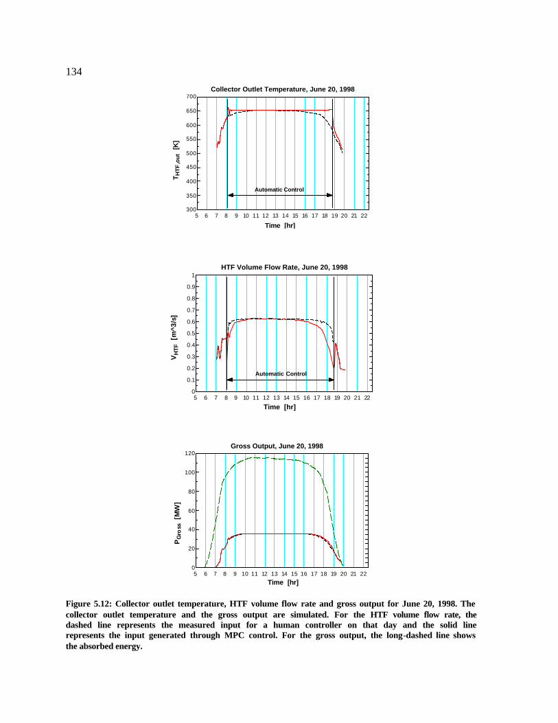
134

5 6 7 8 9 10 11 12 13 14 15 16 17 18 19 20 21 22300

350

400

450

500

550

600

650

700

Time [hr]

T HTF

,out

[K

]

Collector Outlet Temperature, June 20, 1998

Automatic Control

5 6 7 8 9 10 11 12 13 14 15 16 17 18 19 20 21 220

0.1

0.2

0.3

0.4

0.5

0.6

0.7

0.8

0.9

1

Time [hr]

VH

TF [

m^3

/s]

HTF Volume Flow Rate, June 20, 1998

Automatic Control

5 6 7 8 9 10 11 12 13 14 15 16 17 18 19 20 21 220

20

40

60

80

100

120

Time [hr]

PG

ross

[M

W]

Gross Output, June 20, 1998

Figure 5.12: Collector outlet temperature, HTF volume flow rate and gross output for June 20, 1998. The collector outlet temperature and the gross output are simulated. For the HTF volume flow rate, the dashed line represents the measured input for a human controller on that day and the solid line represents the input generated through MPC control. For the gross output, the long-dashed line shows the absorbed energy.

135

5 6 7 8 9 10 11 12 13 14 15 16 17 18 19 20 21 22300

350

400

450

500

550

600

650

700

Time [hr]

T HTF

,out

[K

]

Collector Outlet Temperature, September 19, 1998

Automatic Control

5 6 7 8 9 10 11 12 13 14 15 16 17 18 19 20 21 220

0.1

0.2

0.3

0.4

0.5

0.6

0.7

0.8

0.9

1

Time [hr]

VH

TF [

m^3

/s]

HTF Volume Flow Rate, September 19, 1998

Automatic Control

5 6 7 8 9 10 11 12 13 14 15 16 17 18 19 20 21 220

20

40

60

80

100

120

Time [hr]

PG

ross

[M

W]

Gross Output, September 19, 1998

Figure 5.13: Collector outlet temperature, HTF volume flow rate and gross output for September 19, 1998. The collector outlet temperature and the gross output are simulated. For the HTF volume flow rate, the dashed line represents the measured input for a human controller on that day and the solid line represents the input generated through MPC control. For the gross output, the long-dashed line shows the absorbed energy.

136

5 6 7 8 9 10 11 12 13 14 15 16 17 18 19 20 21 22300

350

400

450

500

550

600

650

700

Time [hr]

T HT

F,o

ut [

K]

Collector Outlet Temperature, December 16, 1998

Automatic Control

5 6 7 8 9 10 11 12 13 14 15 16 17 18 19 20 21 220

0.1

0.2

0.3

0.4

0.5

0.6

0.7

0.8

0.9

1

Time [hr]

VH

TF [

m^3

/s]

HTF Volume Flow Rate, December 16, 1998

Automatic Control

5 6 7 8 9 10 11 12 13 14 15 16 17 18 19 20 21 220

20

40

60

80

100

120

Time [hr]

PG

ross

[M

W]

Gross Output, December 16, 1998

Figure 5.14: Collector outlet temperature, HTF volume flow rate and gross output for December 16, 1998. The collector outlet temperature and the gross output are simulated. For the HTF volume flow rate, the dashed line represents the measured input for a human controller on that day and the solid line represents the input generated through MPC control. For the gross output, the long-dashed line shows the absorbed energy.

137

5 6 7 8 9 10 11 12 13 14 15 16 17 18 19 20 21 22300

350

400

450

500

550

600

650

700

Time [hr]

T HT

F,o

ut [

K]

Collector Outlet Temperature, December 14, 1998

Automatic Control

5 6 7 8 9 10 11 12 13 14 15 16 17 18 19 20 21 220

0.1

0.2

0.3

0.4

0.5

0.6

0.7

0.8

0.9

1

Time [hr]

VH

TF

[m^3

/s]

HTF Volume Flow Rate, December 14, 1998

Automatic Control

5 6 7 8 9 10 11 12 13 14 15 16 17 18 19 20 21 220

20

40

60

80

100

120

Time [hr]

PG

ross

[M

W]

Gross Output, December 14, 1998

Figure 5.15: Collector outlet temperature, HTF volume flow rate and gross output for December 14, 1998. The collector outlet temperature and the gross output are simulated. For the HTF volume flow rate, the dashed line represents the measured input for a human controller on that day and the solid line represents the input generated through MPC control. For the gross output, the long-dashed line shows the absorbed energy.

138The related collector outlet temperature and the gross output, calculated through simulation

with the complex plant model, are the dashed lines in the top figure and in the bottom figure

respectively. The HTF volume flow rate shown as solid line represents the input calculated

through model predictive control. The solid lines in the top and the bottom figure are the

corresponding collector outlet temperature and gross output. The automatic controller is

turned on at 8.05 hr in the morning and turned off at 18.8 hr. The start up and shut down are

assumed to be done by a human. The MPC controller obtains the ability to hold the collector

outlet temperature at a constant set point (653.9 K) for a long time throughout the day. For a

damping of oscillations, the regulator parameters are 20=N , 50=Q and 1000=S for a

sample period of 100=∆ s. A noise free control is assumed and the variances of the

stochastic variables in the estimator are chosen very small. The performance of the automatic

controller is better than the performance of the human controller. However, oscillations occur

when starting the automatic control and when the controlled plant reaches the transient.

Although different regulator parameters were tested, it was not possible to reject these

oscillations. The fact that the MPC controller shows a better performance than the human

controller in generating a constant set point collector outlet temperature, does not improve

the gross output remarkably, as can be seen from the bottom Figure. As an illustration of

efficiency, the absorbed energy is plotted in the graph as well.

In Figure 5.13, the collector outlet temperature and the HTF volume flow rate are

shown for September 19, 1998. Again, dashed lines represent human control and solid lines

represent automatic control. The linear model used to control on that day is different from the

linear model used to control on June 20, 1998 since it was linearized around a different

steady-state solution of the nonlinear model. The MPC controller is turned on at 9.00 hr and

139turned off at 17.8 hr. The regulator parameters are the same as for June 20, 1998. The set

point temperature is 637.2 K. The MPC control action results in a collector outlet

temperature that is held constantly in the set point. Slight oscillations occur before the

automatic controller is turned off. Also in this case, there is no remarkable improvement in

the gross output through automatic control.

In Figure 5.14, the results are shown for December 16, 1998. Again, a different linear

model is applied for MPC control compared to the ones used for the control on a summer or

early fall day. The automatic controller is turned on at 9.00 hr and turned off at 16.00 hr. The

collector outlet temperature set point is 597.3 K, the regulator parameters are the same as

above. The automatic control performance is much better than the human one. The controlled

temperature slightly rises before the controller is turned off. The gross output doesn’t change

much when either human or automatic control is applied.

Finally, a partially cloudy day is considered in Figure 5.15. Since December 14, 1998

was two days before December 16, 1998, considered above in Figure 5.14, the same linear

model and the same controller parameters and set point temperature are taken. The MPC

controller is turned on at 9.00 hr and turned off at 16.00 hr. The automatic controlled

collector outlet temperature is in the set point until the solar energy goes down. The

automatic controller tries to compensate the occurring drop in the collector outlet temperature

through the adjustment of the HTF volume flow rate while reaching its lower bound

/sm0682.0 3, =minHTFV& . Since the MPC controller is now constraint in its control action, it

cannot hold the collector outlet temperature in its set point and the temperature decreases.

However, the control action of the automatic controller results in a collector outlet

140temperature much closer to the set point compared to the human controlled one. There is no

remarkable improvement in the gross output due to automatic controls.

141

Chapter 6

Conclusions and Recommendations

6.1 Conclusions A nonlinear model of the 30 MWe SEGS VI parabolic trough plant has been established. The

model consists of a dynamic model for the collector field and a steady-state model for the

power plant.

First, the collector field model was presented as coupled partial differential equations

for energy. For the implementation in digital machines, a set of ordinary differential

equations was obtained through dicretization of the governing energy PDEs. The calculation

of the absorbed solar energy from the direct normal solar radiation was presented. The

performance of this model was evaluated through a comparison between predicted and

measured data. The model calculations matched the measurement very well.

A steady-state model for the power plant Clausius-Rankine cycle was developed from

measured power plant data and from a report by Lippke (1995) on the power plant design

conditions. Good agreement between the power plant model predictions and measured data

was achieved.

The collector field model and the power plant model were combined to an entire plant

model that was implemented in EES. This plant model was also evaluated through a

comparison between predicted and measured data. It proved to be a useful model for

SEGS VI.

142 A model predictive controller was developed for the SEGS VI plant model. Its task is to

maintain a constant collector outlet temperature on different days of a year by adjusting the

heat transfer fluid volume flow rate while solar radiation changes. The control algorithmic,

which is based on Rawlings and Muske (1993), was introduced on the example of a

simplified model. The automatic controller was implemented in MATLAB. The control

performance was evaluated through simulations for four different days in 1998. The MPC

controller showed the capability to hold the collector outlet temperature close around the

specified set point for a long time during the day. The automatic controller demonstrated a

better control of the collector outlet temperature than the human control. However, the

improvement in the predicted gross output of the power plant due to the better control of the

collector outlet temperature is small.

6.2 Recommendations

Further studies should include the model predictive control strategy with the objective to

maximize the gross output. Controlling both, the HTF volume flow rate and the steam mass

flow rate in the power plant could help improving the daily gross output of the parabolic

trough plant.

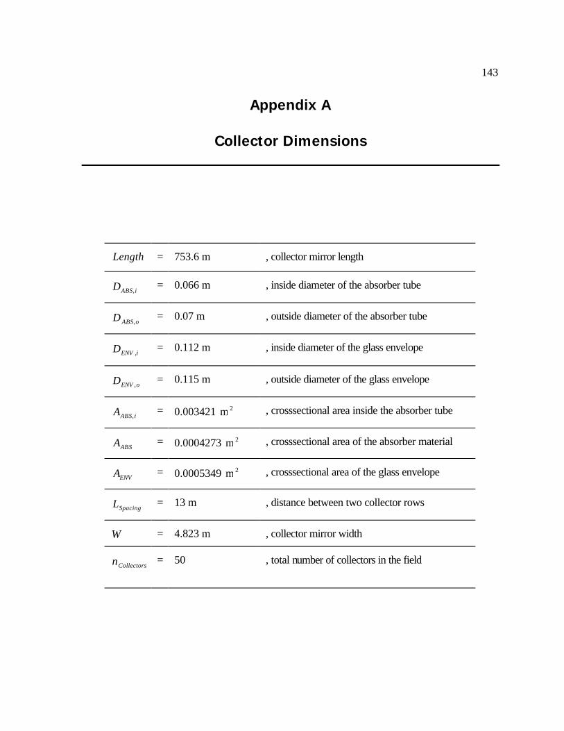
143

Appendix A

Collector Dimensions

Length = 753.6 m , collector mirror length

iABSD , = 0.066 m , inside diameter of the absorber tube

oABSD , = 0.07 m , outside diameter of the absorber tube

iENVD , = 0.112 m , inside diameter of the glass envelope

oENVD , = 0.115 m , outside diameter of the glass envelope

iABSA , = 0.003421 2m , crosssectional area inside the absorber tube

ABSA = 0.0004273 2m , crosssectional area of the absorber material

ENVA = 0.0005349 2m , crosssectional area of the glass envelope

SpacingL = 13 m , distance between two collector rows

W = 4.823 m , collector mirror width

Collectorsn = 50 , total number of collectors in the field

144

145

Appendix B

Nomenclature

A area, m if surface per length or 2m if cross-sectional; state-space model

matrix

Aa , Ba HTF flow fraction for heat exchanger train A or B B state-space model matrix

Ab , Bb HTF flow fraction for reheater A or B C state-space model matrix c specific heat, J/kg

pc specific heat at constant pressure, J/kg·K

D diameter, m; state-space model matrix; quadratic program constraint matrix

d input step disturbance

nd day number

tE equation of time F flow fraction; quadratic program matrix G irradiance, W/m2; quadratic program matrix

ξG state noise dynamics matrix

g gravitational acceleration, m/s2 H quadratic program matrix h specific enthalpy, J/kg; convection heat transfer coefficient, W/m2·K

ux JJ , Jacobian matrix k thermal conductivity, W/m·K L length, m; filter gain matrix

locst LL , standard and local longitude, deg Length collector mirror length m& mass flow rate, kg/s Nu Nusselt number n number P steady-state discrete filtering Riccati matrix

GrossP gross output, W Pr Prandtl number p Pressure, N/m2 Q energy transfer, J; output penalty matrix

ωξ QQ , convariance matrix of ξ and ω

146

Q& heat transfer rate, W

q heat transfer rate per unit length, W/m Ra Rayleigh number Re Reynolds number

mR & mass ratio

pR pressure ratio

νR covariance matrix of ν S input rate of change penalty matrix s specific entropy, J/kg-K T temperature, K t time, s UA overall heat transfer coefficient and area product, W/K u input vector V volume , m3 V& volume flow rate, m3/s v input vector substitute

Nv vector of N future input vectors W collector mirror width, m; quadratic program constraint matrix w state vector substitute x model state vector; shading y output vector z coordinate, m; output vector substitute Greek Letters α thermal diffusivity, m2/s; absorptance

pα profile angle, deg

β volumetric thermal expansion coefficient, K-1 γ fudge factor ∆ sampling period, s

p∆ pressure drop ratio

RHHE pp ∆∆ , pressure drop, N/m2 Q∆ change in the energy transfer, J

V&∆ rate of change in the volume flow rate z∆ length of discrete collector element, m

δ declination, deg ε effectiveness, emissivity η efficiency θ angle of incidence, deg

147

zθ zenith angle, deg µ viscosity, kg/s·m ν kinematic viscosity, m2/s; zero-mean, normal output noise vector ξ zero-mean, normal state noise vector; component of state vector ρ Mass density, kg/m3; specular reflectance; feedback σ Stefan-Boltzmann constant

kΦ regulator objective function value at time k φ latitude, deg Ψ target tracking objective function value τ time constant, s; transmittance

)(τα transmittance-absorptance product ω hour angle, deg; zero-mean, normal state step disturbance noise vector Subscripts ABS absorber Air air Annulus in the annulus absorbed absorbed solar energy amb, ambient ambient, in the environment atm atmospheric bn direct normal beam Col collector Collectors number of collectors Cool cooling water CP condensate pump c cross-sectional; cold fluid convection convection heat transfer d non-manipulable input; discrete-time system matrix END end time ENV envelope Environment environmental Exp expansion vessel eff effective evac evacuated external heat transfer to environment FP feedwater pump gained gained energy Gross gross output HE heat exchanger

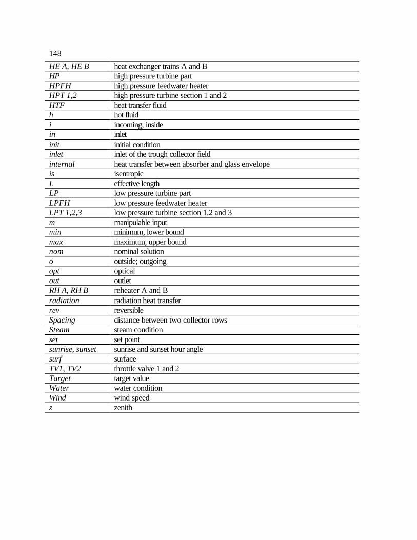
148

HE A, HE B heat exchanger trains A and B HP high pressure turbine part HPFH high pressure feedwater heater HPT 1,2 high pressure turbine section 1 and 2 HTF heat transfer fluid h hot fluid i incoming; inside in inlet init initial condition inlet inlet of the trough collector field internal heat transfer between absorber and glass envelope is isentropic L effective length LP low pressure turbine part LPFH low pressure feedwater heater LPT 1,2,3 low pressure turbine section 1,2 and 3 m manipulable input min minimum, lower bound max maximum, upper bound nom nominal solution o outside; outgoing opt optical out outlet RH A, RH B reheater A and B radiation radiation heat transfer rev reversible Spacing distance between two collector rows Steam steam condition set set point sunrise, sunset sunrise and sunset hour angle surf surface TV1, TV2 throttle valve 1 and 2 Target target value Water water condition Wind wind speed z zenith

149

Overbar, Tilde and Hat

surface average conditions; desired value at steady state

~ perturbation from nominal solution; augmented system matrix ^ estimated value

150

151

References Duffie, J.A and Beckman, W.A. (1991), Solar Engineering of Thermal Processes, John Wiley & Sons, Inc., New York. Iqbal, M. (1983), An Introduction to Solar Radiation, Academic Press Canada, Ontario. Incropera, F.P. and De Witt, D.P. (2002), Introduction to Heat Transfer, John Wiley & Sons, Inc., New York. Pilkington (1996), Status Report on Solar Thermal Power Plants, Pilkington Solar International GmbH, Cologne, Germany. Klein, S.A. (2001), EES Engineering Equation Solver, F-Chart Software, USA Lippke, F. (1995), Simulation of the part-load behavior of a 30 MWe SEGS plant, SAND95-1293, Sandia National Laboratories, Albuquerque, NM. El-Wakil, M.M. (1984), Powerplant Technology, McGraw-Hill, Inc., New York. MathWorks (2001), Using the Optimization Toolbox, The Mathworks, Inc., Natick, MA Kwakernaak, H. and Sivan, R. (1972), Linear Optimal Control Systems, John Wiley & Sons, Inc., New York. Schindwolf, R. (1980), Fluid Temperature Control of Parabolic Trough Solar Collectors, presented at the Joint Automatic Control Conference, San Francisco, Calif., Aug. 13-15, 1980. Rawlings, J.B. and Muske, K.R. (1993), Model Predictive Control with Linear Models, AIChE Journal, 39 (2), 262-287. Rawlings, J.B. (2000), Tutorial Overview of Model Predictive Control, IEEE Control Systems Magazine, 38-52.