Attitude Stabilization of a Biologically Inspired Robotic Housefly

via Dynamic Multimodal Attitude Estimation

Domenico Campolo1 Giovanni Barbera2 Luca Schenato2 Lijuan Pi3

Xinyan Deng3 Eugenio Guglielmelli4

1School of Mechanical & Aerospace Engineering, Nanyang Technological University, 639798 Singapore

2Department of Information Engineering of the University of Padova, 35131 Padova - Italy

3Department of Mechanical Engineering, University of Delaware, Newark, DE - USA

4Biomedical Robotics Laboratory of the Campus Bio-Medico University, 00128 Roma - Italy

d.campolo@ntu.edu.sg

Abstract

In this paper, we study sensor fusion for the attitude stabilization of Micro Aerial Vehicles

(MAVs), in particular mechanical flying insects. Following a geometric approach, a dynamic observer

is proposed which estimates attitude based on kinematic data available from different and redundant

bio-inspired sensors such as halteres, ocelli, gravitometers, magnetic compass and light polarization

compass. In particular, the traditional structure of complementary filters, suitable for multiple

sensor fusion, is specialized to the Lie group of rigid body rotations SO(3). The filter performance

based on a 3-axis accelerometer and a 3-axis gyroscope is experimentally tested on a 2 degrees-

of-freedom support showing its effectiveness. Finally, attitude stabilization is proposed based on

a feedback scheme with dynamic estimation of the state, namely the orientation and the angular

velocity. Almost-global stability of the proposed controller in the case of dynamic state estimation

is demonstrated via the separation principle, and realistic numerical simulations with noisy sensors

and external disturbances are provided to validate the proposed control scheme.

keywords: attitude control on SO(3), separation principle, geometric control, complementary filter-

ing, biologically inspired robots.

1 Introduction

The development of Unmanned Air Vehicles, (UAV), has been a very active area of research for both

civil and military applications. Many remarkable achievements have been obtained with large fixed

and rotary aircrafts, however their use in many tasks is limited by their maneuverability and size. In

order to overcome these limitations, the extraordinary flight capabilities of insects have inspired the

design of small Micro Aerial Vehicles (MAVs) and in particular of inch size robots with flapping wings

1

mimicking real flying insects [1]. Their unmatched maneuverability, low fabrication cost and small size

make them very attractive for cost-critical missions in environments which are impenetrable for larger

size UAVs such as helicopters or airplanes. Moreover, the latest progresses in insect flight aerodynamics

[2] and in micro-technology [3] are providing sufficient tools to fabricate flying insect micro-robots, as

shown by the recent take-off of flapping flight robotic insect [4]. Although many problems remain to

be solved in terms of fabrication and electromechanical design, the next fundamental challenge to be

undertaken is the design of control architectures and algorithms to control and navigate flapping flight

robotic insects. It has been observed by biologists that insects can control the generation of forces and

torques by modulating the wing kinematics trajectories [2] [5]. This observation has suggested the use of

averaging theory tools and a bio-inspired parameterization of the wing kinematics to decouple the wing

control design from the attitude control design [6] [7]. This approach has been shown successful also in

other bio-mimetic forms of locomotion such as fish swimming [8], and greatly simplifies the design of an

autonomous navigation systems, since it naturally leads to a hierarchical architectures [7].

Based on these considerations, in this paper, we focus on the design of attitude control which uses

as inputs the signals coming from bio- inspired sensors such as ocelli, halteres, magnetometers and

gravitometers. The ability of controlling attitude in a robust and stable manner is fundamental for

the design of path planning and navigation control schemes. Previous work exists in this context. For

instance, in [9] the authors propose a static output feedback scheme for hovering recovery, however

this scheme is sensitive to measurement noise and external disturbances, moreover cannot be easily

extended to attitude maneuvering or control schemes based on body orientation. Rifai et al. [10]

provide an attitude control scheme which takes into account saturation limits, but they do not consider

sensors and assume to have access to exact body orientation and angular velocity. Finally, Epstein et

al. [11] propose a dynamic output feedback schemes based on a linearized model of the insect dynamics

suitable for longitudinal control or other simple flight modes, but not for more aggressive maneuvers.

Here, we propose a dynamic output feedback control scheme that is globally stable and that is based

on state estimation from redundant measurements, make it more robust to external disturbances and

measurement noise. In particular, we show that we can decouple the orientation estimation problem

from the attitude control problem. Although, this separation principle is classical for linear dynamical

systems, it is hard to be guaranteed for general nonlinear systems and in particular for the Lie group

of rigid body orientations SO(3). Although this scheme has been specifically designed for robotic flying

insects with bio-inspired sensors, it is rather general and can be used also for more traditional UAVs as

long as the output signals are “linear” in the rotation matrix, as explained later. In fact, this scheme

has the advantage to be globally stable differently from more traditional control strategies based on

Extended Kalman Filters.

As for the outline of the paper, Section 3 briefly describes the attitude dynamics of a robotic fly-

ing insect and reviews navigation sensory system of real insects. Section 4 presents a complementary

filter for sensor fusion as well as the experimental validation of its performance. Section 5 proposes a

control feedback based on the dynamic attitude estimation which is proven to be globally stable via

2

the separation principle, and it is tested using realistic numerical simulations. Before proceeding some

mathematical background is presented.

2 Mathematical Background

This section briefly describes the notation and several geometric notions that will be used throughout

the paper. For additional details, the reader is referred to texts such as [12, 13, 14, 15, 16].

2.1 Basic Definitions

As shown in [12, 13], the natural configuration space for a rigid body is the Lie group SO(3), i.e. the

configuration of a rigid body can always be represented by a rotation matrix R, i.e. a matrix such that

R−1 = RT and detR = +1.

Consider now the coordinate frames R3S and R3

B :

• R3S ≈ R3: the space coordinate frame, or initial configuration frame.

• R3B ≈ R3: the body frame, which is attached to the body (can be thought of as defined by the

sensors sensitive axis), initially coincident with the space frame.

An element R of SO(3) can be thought of as a map from the body frame to the space frame, i.e.

R : R3B → R3

S .

A trajectory of the rigid body is curve R(t) : R → SO(3). The velocity vector R is tangent to the

group SO(3) in R but, as shown in [12, 13], rather than considering R, two important quantities are

worth to be considered:

• R RT : representing the rigid body angular velocity relative to the space frame;

• RT R: representing the rigid body angular velocity relative to the body frame.

These are both elements of the Lie algebra so(3), i.e. the tangent space to the group SO(3) at the

identity I.

Elements of the Lie algebra are represented by skew-symmetric matrices. Systems on Lie groups

described in terms of body (space) coordinates are called left-invariant (right-invariant).

Left-invariance: let R1(t) be a trajectory of a rigid body relative to a space frame R3S1

. Consider a

change of space frame G : R3S1 → R3

S2, now R2(t) = GR1(t) represents the same trajectory but with

respect to the new space frame. It is straightforward to verify that RT2 R2 = RT1 R1, i.e. the angular

velocity relative to the body frame RT R does not depend on the choice of space frame.

Right-invariance: similarly, it can be shown that the angular velocity of a rigid body relative to a

space frame R RT does not depend on the choice of coordinate frame attached to the body.

3

In the case of SO(3), there exists [13] an isomorphism of vector spaces · : so(3)→ R3, referred to as

hat operator, that allows writing so(3) ≈ R3. For a given vector a = [a1 a2 a3]T ∈ R3, we write:

· : a =

a1

a2

a3

−→

0 −a3 a2

a3 0 −a1

−a2 a1 0

= a (1)

Denote (·)∨ : R3 → so(3) its inverse, referred to as vee operator:

(·)∨ : a =

0 −a3 a2

a3 0 −a1

−a2 a1 0

−→a1

a2

a3

= (a)∨ (2)

The Lie algebra is equipped with an operator, the Lie brackets [·, ·] which is defined by the matrix

commutator:

[a, c] = a c− c a = a× c (3)

where a, c ∈ R3, a, c ∈ so(3) and × is cross product in R3.

Given a finite-dimensional vector space V , let V ∗ be its dual space, i.e. the space whose elements

(covectors) are linear functions from V to R. If σ ∈ V ∗, then σ : V → R. Denote the value of σ on

v ∈ V by 〈σ,v〉, i.e. the pairing operator 〈·, ·〉 : V ∗ × V → R.

If V = Rn then V ∗ ' Rn. For all v ∈ V and σ ∈ V ∗ ' Rn then

〈σ,v〉 = σTa

〈 σ, v 〉 = 12trace( σT v )

(4)

2.2 Metric properties of SO(3)

In what follows necessary background and geometric tools are reviewed in order to define a norm (a

distance) on SO(3). This will be used later to prove convergence of the proposed feedback.

On a general manifold M , a positive definite quadratic form 〈〈ξ1, ξ2〉〉TxM defined on any tangent

space TxM 3 ξ1, ξ2 (the space tangent to M in x ∈ M) is called a Riemannian metric [12]. It is the

equivalent of the scalar product in Rn, can be used to measure the distance between different points of

a manifold, in mechanics a metric is tightly linked to the definition of kinetic energy [16]. A metric is

extra structure, does not come with the manifold. Many different metrics, i.e. many different distance

measures, can be defined on the same manifold [12].

Lie groups are, by definition, manifolds and therefore are entitled to posses metric properties. Lie

groups, in particular SO(3), are structured in such a way that some metrics naturally1 arise. A left-

invariant metrics does not depend on the choice of the space frame, i.e. it only needs to be defined on

the Lie algebra and then it can be left-translated to the tangent space at any other group element:

〈〈R a, R c〉〉TRSO(3) = 〈〈a, c〉〉so(3)

1 Natural means that it does not depend on a particular choice of coordinates.

4

where R ∈ SO(3) and a, c ∈ so(3).

Still, there many choices for a metric in the Lie algebra, as many as there are positive definite

matrices P :

〈〈a, c〉〉so(3)∆= aTP c

where a, c ∈ R3 correspond to a, c ∈ so(3) as in Eq.(1). However, there only exists one choice (up to a

coefficient, [12, 13, 16, 17]) when the metrics needs to be bi-invariant (i.e. both right- and left-invariant):

〈〈a, c〉〉so(3)∆= aT I c = aT c = 〈a, c〉 (5)

where I is the 3× 3 identity matrix.

Two main results provided in [17] are:

- the existence of a natural norm2 on SO(3):

‖R‖SO(3) = 〈〈φR, φR〉〉1/2so(3) = ‖φR‖R3 (6)

- and a formula for computing its time derivative on the Lie algebra so(3):

12d

dt‖R(t)‖SO(3) = 〈〈φR, RT R〉〉so(3)R

T >so(3) (7)

where φR ∈ so(3), also referred to as logR, is defined as the angular velocity that takes the rigid body

from I to R ∈ SO(3) in one time unit, see [13] for details on the logarithmic map:

φR = logR =θR

2 sin θR(R−RT ) (8)

where, for trace(R) 6= −1, θR satisfies 1 + 2 cos θR = trace(R) and ‖φR‖2 = θ2R, and the Rodrigues’

formula:

R = exp(φR) = I + αR φR + βR φ2

R (9)

where αR = ‖φR‖−1 sin ‖φR‖ and βR = (1− cos ‖φR‖)‖φR‖−2.

3 BIOLOGICALLY INSPIRED ROBOTIC HOUSEFLY

In this section we review the most important features of a Micromechanical Flying Insect, summarizing

some of the results presented in [6][7].

3.1 Dynamics of the Micromechanical Flying insect

Insect flight dynamics is still a very active area of research. In particular, there is great interest in

understanding the unsteady state nature of flapping wings aerodynamics, which is believed to be source

of the high maneuverability of insect flight as compared to fixed-winged vehicles and helicopters [18]. A2Which measures the distance between R and the identity I.

5

detailed discussion of flying insect aerodynamics and modeling is beyond the scope of this paper, and

we address the interested readers to the recent paper by Deng et al. and references therein [6]. Here,

we simply summarize some results relevant to our discussion on attitude stabilization.

Since the mass of the wings is negligible with respect to the body mass, the dynamics of a flying insect

can be modeled as the dynamics of a rigid body subject to external forces and torques. In particular,

as long as attitude is concerned, the dynamics is described by:

Jω = τ aero − ω × Jω (10)

where J is the moment of inertia of the insect, τ aero is the total external torque with respect to the

insect center of mass in the body frame due to the aerodynamic forces generated by the flapping wings,

and ω is the angular velocity with respect to the body.

The dynamics of (10), affine with respect to the forcing input τ aero, can be averaged out as in [7].

The time varying components of the torque can be neglected while the mean value of the torque τFB

will be used as the feedback (FB) term for attitude stabilization. As this term depends upon the current

orientation R and the current angular velocity ω, the averaged attitude dynamics of a mechanical flying

insect are described by the system R = R ω

ω = J−1(Jω × ω + τFB(R,ω))(11)

where the . hat operator transforms the ω vector into a skew-symmetric matrix ω and (R,ω) is an

element of SO(3) × so(3), i.e. the product space of the Lie Group SO(3) of rigid body rotations and

its Algebra so(3).

3.2 The Sensory System of Flying Insects

The highly specialized sensory system of flying insects is at the base of their extraordinary flying per-

formance. In fact flying insects can rely on an heterogeneous set of redundant sensors for controlling

flight maneuvers and navigate the environment. Redundancy is the key to robustness. Some of these

sensors represent a rich source of inspiration for the design of mechanical flying insects [19][6] and they

motivate the control strategy proposed in this work.

3.2.1 Halteres

The halteres are club-shaped small appendages behind each wing that oscillate in anti-phase with respect

of the wing, as shown in Fig. 1. The plane of oscillation is slightly tilted toward the tail of the insect to

be able to measure Coriolis forces along all three body axes [20]. The halteres function as tiny gyroscopes

and through appropriate signal processing [21] they can reconstruct the body angular velocity vector:

yhl = ω (12)

Recently, preliminary prototypes of micro-electromechanical halteres have been fabricated and have

shown promising results [22].

6

Figure 1: Photo of a fly haltere. Courtesy of [23].

3.2.2 Mechanoreceptors

Many parts of the insect body such as wings, antennae, neck and legs are innervated by campaniform

sensilla. These cells can measure and encode pressure forces when they are stretched or strained [24].

For example sensilla at the base of wing hinges can measure aerodynamic forces, which are used to fine

tune the wing motion. Similarly, the sensilla on the legs might be used to measure the gravity sensor,

thus acting as a gravitometer. Therefore, in static conditions, insect can measure the gravity vector

with respect to the body frame, i.e.

yg = RTg0 (13)

where g0 are the (known) gravity vector components, measured with respect to the fixed frame. In

non-static conditions, also noninertial accelerations add-up to the output of mechanoreceptors, as a

form of disturbance. Combining information from mechanoreceptors and halteres (sensor fusion) can

greatly alleviate the effects of such disturbances.

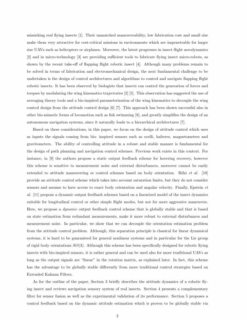
3.2.3 Ocelli

The ocelli are three additional light-sensitive organs located at the vertices of an imaginary triangle on

the middle of head of the insect as shown in Fig. 2, and provide signals that are used for stabilization

7

with respect to rapid perturbations in roll and pitch [19]. In fact, these sensors collect and measure light

intensity from a portion of the sky, and they estimate the position of the sun with respect to insect body

by comparing the signals from the left and right ocelli to estimate the roll angle, and by comparing the

signal from the forward-looking ocellus with the mean of the signals from the left and the right ocelli to

estimate the pitch angle [25].

Figure 2: Photo of fly’s head showing compound eyes and the ocelli with its three photoreceptors.

Courtesy of [26].

3.2.4 Compound eyes

The compound eyes of the insects are an advanced vision system that processes different types of signals

needed for the optomotor systems. In fact they can process the visual stimuli to estimates angular

velocities thanks to large-field neurons that are tuned to respond to the specific patterns of optic flow

that are generated by yaw, roll and pitch [27], as well as body orientation and position by higher level

visual processing like object fixation and landmarks detection for navigation and path planning [11].

However, such signals requires quite a specialized signal processing system that might not be necessary

for attitude stabilization, which is the objective of this work. However, the dorsally directed (upward-

looking) regions of the compound eyes of many insects are equipped with specialized photoreceptors

that are sensitive to the polarized light patterns that are created by the sun in the sky. More precisely

insects can measure their orientation relative to the direction of the light polarization: p0 ∈ R3, as:

yp = RTp0 (14)

Differently from the ocelli, the light polarization direction is not affected by light intensity. Bio-inspired

polarized light compasses are easier to fabricate that the full insect visual system, and have been suc-

cessfully fabricated and used for robot navigation [28] and it is relevant to the flight control design

proposed in this work.

8

3.2.5 Magnetic compass

Recent studies indicate that some insects also can detect the earth magnetic and it is used to maintain

a desired heading direction [29]. Similarly to the light polarization sensor, we can argue that insect can

measure the components of the magnetic field with respect to the body as follows:

ym = RTb0 (15)

where b0 ∈ R3 is the direction of magnetic field relative to the fixed frame. A possible electromechanical

implementation of a magnetic compass suitable for small size vehicles is given in [30].

4 SENSOR FUSION VIA COMPLEMENTARY FILTERS

The sensory system of real insects is clearly redundant, e.g. kinematic quantities such as the angular

velocity are derived from more than one sensor. Information from different sensors is then ‘fused’

together. Complementary filters traditionally arise in applications where redundant measurements of

the same signal are available [31] and the problem is combining all available information in order to

minimize the instrumentation error.

For sake of simplicity, consider only two sensors, s1 and s2, providing readings of the same quantity,

e.g. the angular velocity ω, with different noise characteristics, i.e. s1 = ω+ n1 and s2 = ω+ n2, where

‖n1‖ < ‖n2‖ at high frequency while ‖n2‖ < ‖n1‖ at low frequency. Then an low-pass filter L(s) and

its complementary high-pass filter H(s) = 1− L(s) can be used to fuse information

sfusion = s1H(s) + s2L(s) = ω + n2L(s) + n1(1− L(s)) (16)

from two or more sensors (e.g. halteres, ocelli and compound eyes). The cut-off frequency of the filter

L(s) can be chosen so that the spectral content of n2L(s) + n1(1− L(s)) will be less than the spectral

content of n1 or n2 [31].

The kinematic variable ω is dynamically unaffected by the filter. The estimated variable (i.e. the

output of the filter) is related to the input variable via a purely algebraic relation in the time domain

and no dynamics are involved in the noiseless case. Such filters can be safely used in feedback loops to

fuse readings of the same kinematic variable from different sensors since no extra dynamics is added to

the overall system and stability (which involves noiseless conditions) is not affected.

Complementary filters can be generalized to fuse information deriving from sensors when the sensed

variables are related by differential equations, e.g. position and speed. In these cases, the filter introduces

some dynamics between the estimated output and the sensed inputs.

The differential equations relating the sensed variables may be nonlinear, this is typically the case

when attitude is concerned. Theory of complementary and Kalman filters has been traditionally used

to design attitude filters. Although the Kalman filters can be extended (EKF) to nonlinear cases, they

fail in capturing the nonlinear structure of the configuration space of problems involving, for example,

9

rotations of a rigid body, and most importantly, they can run into instabilities. On the other hand,

nonlinear filters [32], in particular complementary filters, can better capture such a nonlinear structure.

4.1 Dynamic Attitude Estimation

As an example of use of complementary filters when different kinematic variables are involved, consider

the linear case of a rotational mechanical system with one degree of freedom (θ). As shown in [31],

complementary filters such as the one represented in Fig. 3 are traditionally used to fuse information

available from both angular position sensors and tachometers, respectively θsens and ωtacho. Let θ∗ be

the estimate of θ. The filter gain k in Fig. 3 determines the transition frequency of the filter after which

the data from the tachometer (ωtacho) are weighted more whereas before the transition frequency data

from the position sensors (θsens) are predominant on the dynamic equation (the integrator 1/s). The

optimal value for k is in fact determined from the spectral characteristics of measurement noise [31].

!sens

k

+ 1s

+ _

!*"tacho

Figure 3: Linear complementary filter for a rotational mechanical system with one degree of freedom.

Differently from previous example, SO(3) is a nonlinear space and that is where the advantages

of a geometric approach can be fully appreciated. Besides nonlinear dynamics, the very definition of

estimation error requires caution. In the linear case e = θ−θ∗ is a typical choice while quantities such as

R−R∗ with R,R∗ ∈ SO(3) are no longer guaranteed to belong to SO(3). Following [17], the estimation

error will be defined as E = RTR∗.

A complementary filter on SO(3) was presented in [33] for dynamic attitude estimation. Main

definition, theorem and related lemmas are reported in Appendix A for convenience, the interested

reader can refer to [33] for the proof.

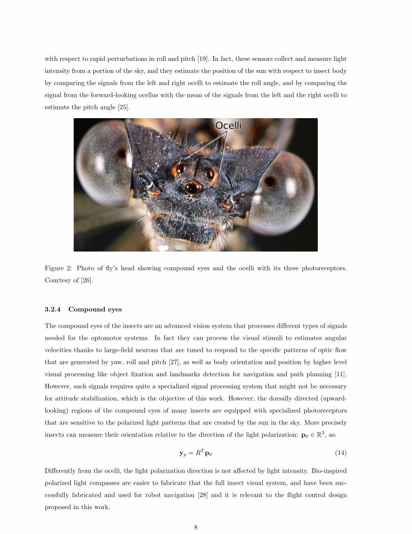
A block diagram of the filter, for the specific case of interest, is shown in Fig. 4. Raw data from

gyroscopes (ωgyr), from accelerometers (g) and from magnetometers (b) (i.e. a total of 9 channels) are

fused together to provide an estimate of the orientation (R∗). The filter also uses two initial readings g0

and b0 respectively from accelerometers and magnetometers. The orientation matrix R∗ can be initially

set to any appropriate value (e.g the 3× 3 identity matrix) in the integration block.

As a final note, in linear cases such as in Fig. 3 all the variables belong to the same space Rn. In the

nonlinear filter in Fig. 4, variables in different nodes of the block diagram belong to very different spaces,

some linear (so(3)) and some nonlinear (SO(3)). The adopted geometric approach leads to recognize

how sensor fusion naturally occurs on the linear space of angular velocities, i.e. the Lie algebra so(3).

10

1s

*

b

g

×R*T

b0

g0×

.

+

kg

kb

R*

b*

g*

b×b*

g×g*

!* !*^ R* = R* !*^.!gyr

Figure 4: Complementary filter for dynamic attitude estimation.

4.2 Numerical Implementation

The filter in Fig. 4, in principle, can be directly implemented in simulation environments such as

MATLAB/ Simulink from MathWorks Inc. Any digital implementation of the filter would i) transform

the filter in a discrete-time one with time sequence tn and ii) necessarily introduce numerical errors.

The main risk is that, as numerical errors accumulate, quantities such as R∗n = R∗(tn) are likely to

drift away from SO(3), i.e. detR∗n very different from 1 and/or R∗Tn R∗n very different from the identity

matrix I. This can be avoided by considering that data from analog sensors are typically acquired via

DACs (Digital to Analog Converters) with a fixed sampling time, let this sampling time be ∆T . In the

time interval tn ≤ t < tn+1 = tn + ∆T , data from sensors can be assumed constantly equal to the last

sampled value. This allows computing R∗n+1 via the Rodrigues’ formula [13] as:

ω∗n = ωn + kg(gn × (R∗Tn g0)) + kb(bn × (R∗Tn b0))

αn = sin ‖∆T ω∗n‖ / ‖∆T ω∗n‖

βn = (1− cos ‖∆T ω∗n‖) / ‖∆T ω∗n‖2

R∗n+1 = R∗n

(I + αn∆T ω∗n + βn∆T 2ω∗2n

) (17)

which is guaranteed not to drift away from SO(3).

4.3 Experimental Tests of Attitude Estimation

In this section we present some experimental results relative to attitude estimation based on the com-

plimentary filter given by Equations (17).

4.3.1 Experimental Setup

A circuit board equipped with a pair of IDG-300 dual-axis gyroscopes (InvenSense) and one 3-axis

ADXL330 accelerometer (Analog Devices) was mounted on a holder and set free to rotate about the

11

Figure 5: The support used to perform the combined roll/pitch motion. The body-fixed coordinate

system is also shown.

roll (x) and pitch (y) axis (see Fig. 5). The holder included two MAE-3 US-Digital angular sensors

to measure exact angular displacement. The accelerometers are used to measure the static gravity

acceleration, while the gyroscopes provide the angular rate with respect to the three axes in the body

reference frame.

4.3.2 Results

According to the reference frame presented in Fig. 5, and adopting the yaw-pitch-roll Euler angles

(ZYX), the rotation matrix R ∈ SO(3) can be considered as a map from the body-fixed frame to the

space frame given by the sequential rotation about the Zb, Yb and Xb axis:

R =

r11 r12 r13

r21 r22 r23

r31 r32 r33

= Rx(−φ)Ry(−θ)Rz(−ψ), (18)

being φ, θ and ψ the roll, pitch and yaw angles, respectively. Since this map is surjective, with the only

exception of the singularity in θ = π/2 for the pitch angle, one can directly evaluate φ, θ and ψ invert

Eqn. (18), and thus immediately compare the true angular position measured by the position sensors

mounted on the holder with the estimated angles from the complimentary filter. Inverting Eqn. (18)

12

yields

θ = − arcsin(r31)

φ = atan2( r32cos(θ) ,

r33cos(θ) )

ψ = atan2( r21cos(θ) ,

r11cos(θ) )

(19)

The matrix RT (t)R∗(t) is guaranteed to converge to the identity matrix I for any initial condition,

i.e. the estimated orientation R∗(t) converges to the true orientation R(t), the initial condition of the

complementary filter. In the experiments the initial orientation R∗(t0), was set to be different from the

true R(t0) in order to evaluate the speed of convergence. The results of attitude estimation from the

! " # $ % & ' ( ) * "!!#

!"

!

"

#

+,--./01-2.!.34/56

! " # $ % & ' ( ) * "!!"

!!7&

!

!7&

89:2.3;6

</=./01-2.".34/56

.

.

/>8?/-./01-2

1@4,A/>>

1@4,.,0-@

/>>.,0-@

Figure 6: Comparison between the actual roll angle (top) and pitch angle (bottom) and three different

estimations evaluated using the only accelerometers data, the only gyroscopes data or both.

complementary filter are shown in Fig. 6 and the associated sensor readouts are shown in Fig. 7 and 8.

The plots show rapid convergence of the estimated angles to the true angles in the first half second of

the experiments when the body frame is kept fixed, and then they remain very close to the true angles

also during the body motion. The effectiveness of sensor fusion is best appreciated by removing either

the gyros or the accelerometers from the filter. In the first case, the removal of the gyros results in an

evident low pass behavior of the estimated angles which exhibit a time lag as compared to the true angle.

Differently, if only gyros are used, the estimated angles have rapid response to body motion, but they

incurs in a drift that overtime leads to large offsets as compared to the true angles. The complementary

filter, as explained above, fuse the benefits from both sensor modality giving rise to a filter with a very

13

! " # $ % & ' ( ) * "!!"

!

"+,-./01/23423

56617189:

! " # $ % & ' ( ) * "!!"

!

"

5661;189:

! " # $ % & ' ( ) * "!!"

!

"

5661<189:

Figure 7: Accelerometers readouts. Readings are normalized with respect to gravity acceleration g.

0 1 2 3 4 5 6 7 8 9 10−5

0

5

Gyr

o x

[rad/

s]

0 1 2 3 4 5 6 7 8 9 10−2

0

2

Gyr

o y

[rad/

s]

0 1 2 3 4 5 6 7 8 9 10−2

0

2

time [s]

Gyr

o z

[rad/

s]

Figure 8: Gyroscopes readouts.

14

high bandwidth.

5 ATTITUDE STABILIZATION VIA THE SEPARATION

PRINCIPLE

In this section, results of traditional attitude control are first reviewed and then applied to derive a

control law based on state feedback. Since in the application of interest the state of the system is

not known and only an estimation of the current state can be used as feedback, it is natural to wonder

whether dynamic output feedback control preserves the stability properties of the state-feedback control,

i.e. whether the separation principle holds. Maithripala et al. [34, 35] proved that the separation

principle also holds in the general case of compact Lie Groups and therefore also for SO(3). For the

reader’s convenience this general result is restated in terms of SO(3) in the Appendix B. In this section,

results from [34, 35] are specialized to SO(3), the Lie Groups of rigid body rotations, and traditional

state feedback control is combined with the dynamic attitude observer presented in [33].

5.1 Attitude Control via State Feedback

Traditionally, control of (11) is performed via passivity-based arguments. Maithripala et al. [34] show

that the system (11) can be stabilized by a state feedback torque τFB(R,ω) which consists of a conser-

vative part, derived from a potential (also referred to as “error”) Morse3 function U : SO(3)→ R, and

a dissipative (Rayleigh-type) part:

τFB(R,ω) = −J (RT gradU + kωω)∨ (20)

where gradU , the gradient of the function U(R). Differently from the differential dU , the gradient

gradU depends on the geometry of the space itself. The gradient is in fact defined by the following

identities:U(R) = 〈dU,R ω〉

= 〈RT dU, ω〉

= 〈〈RT gradU, ω〉〉so(3)

(21)

where, for a vector space V and its dual V ∗, 〈·, ·〉 : V ∗ × V → R is the pairing operator and 〈〈·, ·〉〉V :

V × V → R is the inner product defined via a proper isomorphism J : V → V ∗ as 〈〈a,b〉〉V = 〈Ja,b〉V ,

see [33, 34, 35]. In Mechanics, a natural isomorphism J is provided by the inertia tensor (constant in

body coordinates) and so the gradient is determined by:

RT gradU = J−1RT dU (22)

Therefore, the problem of stabilizing (11) is reduced to defining a potential function U(R) on SO(3)

with a nondegenerate critical point in the desired configuration R ∈ SO(3). To this end, a commonly

3A Morse function is function whose critical points are non-degenerate [16].

15

used potential function, first introduced by Koditschek in [36], on SO(3) is:

U(R) ∆=12trace(K(I − RTR)) (23)

where K is a symmetric 3 × 3 matrix with eigenvalues {k1, k2, k3}. Once the potential function U(R)

is defined, the gradient (and therefore the feedback torque) can be computed as in [37] via the time

derivative of the error function:

U(R) = 12trace(K(−RT R))

= 12trace(−KRTR ω)

= 12trace(skew(KRTR)T ω)

= 〈skew(KRTR), ω〉

(24)

where skew(A) = 12 (A−AT ). This allows computing RT gradU from (22):

RT gradU = J−1skew(KRTR) (25)

Convergence properties of systems like (11) when the state feedback (20) is used can be found in

[34, 35], here briefly restated for the case of interest. The proof is based on La Salle’s principle [15]

and involves a function V = U(R) + 12 〈〈ω, ω〉〉so(3)as well as a set S ⊂ SO(3) × so(3) defined as

S = {(R,ω)|V = 0}.

The sign of V is studied as follows:

V = U(R) + 12 ω

TJω + 12ω

TJω

= U(R) + ωTJω

= U(R) + ωT (Jω × ω + τFB)

= U(R) + ωT τFB

= U(R) + 〈〈J−1τFB , ω〉〉so(3)

(26)

since ωT (Jω × ω) = 0 for all ω ∈ R3.

Considering (22) and (20), then:

V = 〈〈RT gradU, ω〉〉so(3) + 〈〈J−1τFB , ω〉〉so(3)

= −kω‖ω‖2(27)

which implies S = {(R,ω)|ω = 0} and

〈〈RT gradU, ω〉〉so(3) + 〈〈J−1τFB , ω〉〉so(3) ≤ 0 (28)

where the inequality is strict for all (R,ω) /∈ S, implying asymptotic convergence. This satisfies the

assumption A.1 of Lemma 3 in Appendix B.

In order to perform attitude stabilization of the system (11) via state feedback (20), the current

attitude R and angular velocity ω need to be available.

Angular velocity can be directly measured from gyroscopes (for example fusing signals from halteres,

ocelli and compound eyes) while attitude can be estimated from mechanoreceptors and magnetic compass

sensors, as shown next.

16

5.2 Dynamic Attitude Estimation Feedback

In this section, previous results on attitude control via state feedback and the dynamic attitude observer

are coupled via the separation principle, restated in Appendix B.

The full dynamic equations for the proposed attitude stabilization system are:

R = R ω

ω = J−1(τFB(R∗,ω∗)− ω × Jω)attitude controller

R∗ = R∗ ω∗

ω∗ = ωgyr + kb(b× b∗) + kg(g × g∗)dynamic observer

(29)

The first two equations represent the system dynamics (11) with a feedback τFB similar to (20) except

that it is based on the estimates (R∗ and ω∗) of the current orientation and angular velocity, instead

of the actual values (R and ω). The last two equations represent the dynamics of the observer (A-5) in

Appendix A where, without loss of generality, only the minimum number of independent fields (b and

g) is used.

Besides proving almost-global asymptotic stability of the proposed observer, Theorem 1 in [33]

(reported in Appendix A) also provides an upper bound of the attitude estimation error E, defined as:

E = RTR∗ (30)

based on the natural Lyapunov function [17] of the estimation error:

W (E) =12‖E‖2SO(3) =

12‖φE‖2 (31)

where φE is defined via the logarithmic map as φE = logE.

One of the outcomes of Theorem 1 in [33] is the existence of real number η > 0 such that, if the

initial estimation error E(0) is such that traceE 6= −1 (i.e. ‖φE‖ < π which is almost globally verified,

see Remark 1 below), then a bound for the Lyapunov function is

0 < W (E) < W (E(0)) e−ηt

for all t > 0. This translates, via the (31), into an upper bound for the attitude tracking error:

‖φE‖ < c‖φE(0)‖e−λt (32)

where c = W (E(0))/‖φE(0)‖ and λ = η/2. This satisfies assumption A.2 of Lemma 3 in the appendix.

In order to apply the separation principle, rewrite (29) as

R = R ω

ω = J−1(τFB(R,ω)− ω × Jω) +ψ(R,ω,q)

R∗ = R∗ ω∗

ω∗ = ωgyr + kb(b× b∗) + kg(g × g∗)

(33)

17

where ψ(R,ω,q) represents the term J−1(τFB(R∗,ω∗)− τFB(R,ω)). This is possible because ω∗ is a

(linear) function of R, ω and R∗; R∗ can in turn be written as RRTR∗ = RE and E is parameterized

by q ∆= φE .

Since φ(R,ω,q) is linear in ω and SO(3) is a compact Lie group, then assumption A.3 of Lemma 3

in the appendix is also automatically satisfied, see [35, Assumption 3] for details. Recalling that also

assumptions A.1 and A.2 in Lemma 3 where satisfied (respectively in (28) and (32)), then Lemma 3

guarantees that the system (29) almost globally stabilizes the attitude at (R, 0) ∈ SO(3) × so(3) and

that convergence is asymptotic.

Remark 1 (π-rotations) The chosen Lyapunov function (31) proves convergence almost for all pos-

sible initial estimation errors E(0). A question arises: what can be said about the initial configurations

which are left out? Note first that, as clear from the definition of the logarithmic map, any configuration

can be reached via a rotation about some axis by an angle less than or equal to π. The only configurations

left out by the chosen Lyapunov function are those such that trace(E) 6= −1, i.e. such that ‖φE‖ = π.

Such configurations correspond to the set of rotations about an arbitrary axis by an angle exactly equal

to π and will be referred to as π-rotations.

The presence of unstable equilibria is inherently related to π- rotations. As a simple example, for the

needle of a magnetic compass, the North direction is a stable equilibrium while the South direction

(a π-rotation from the North) is an unstable one. In practice, due to the presence of noise, unstable

equilibria are not an issue.

5.3 Simulation results

The housefly body is modeled as an ellipsoid with mass m = 10mg and moment of inertia J =

diag{Jx, Jy, Jz}, where Jx = 0.13 · 10−7kg m2, Jy = 0.16 · 10−7kg m2 and Jz = 0.226 · 10−7kg m2. Three

independent sensors are considered for the attitude estimation: a 3-axis gravitomer which measures the

gravity vector4 components with respect to the body frame, a 3-axis magnetometer which measures the

geomagnetic field vector5, and a 3-axis gyroscope with measures the angular velocity vector. Readouts

from the gravitometer, the magnetometer and gyroscope are simulated as follows:

ωgyro = ω(t) + w1(t)

gmeas(t) = P (s)RT (t)b0 + w2(t)

bmeas(t) = RT (t− τd)g0 + w3(t)

(34)

where ω(t) and R(t) obey to Eqn. (29), wi(t) ∈ R3 are zero-mean independent additive gaussian noises

with variance σ21 = 0.6, σ2

2 = σ23 = 0.2. With a little abuse of notation we indicate with z(t) = P (s)y(t)

the filtered version of the signal y(t) where P (s) is the transfer function of a second order low-pass

filter which models the dynamics of the accelerometers inside the gravitometer. The variable τd (set

4normalized without loss of generality to g0 = [0 0 1]T with respect to a right-handed space frame5normalized w.l.o.g. to b0 = [1 0 0]T

18

to 30ms in the simulation) represents a delay in the magnetic sensor outputs which models possible

HW/SW measurement signal processing time. In the simulations we used P (s) = ω2n

s2+2ξωns+ω2n

, where

ωn = 30, ξ = 0.5. The control torque τFB(R∗,ω∗) used in (33) was designed based on (20) where kω = 8

and K = 30 I ∈ R3×3.

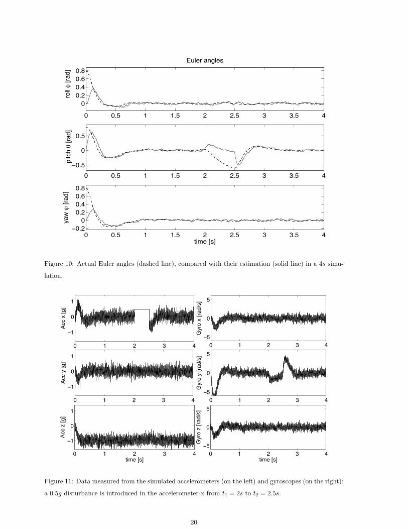
Some closed loop simulations results are shown in Fig. 10. During the simulation the body, starting

from an orientation R(0) 6= I, namely φ0 = θ0 = ψ0 = π/4, is driven by the control torque to the desired

position R(t) = I. A block diagram illustrating the control algorithm6 is presented in Fig. 9.

Figure 9: Schematic design of the control algorithm implementation.

Because R∗(0) is chosen to be the identity matrix I, the estimation initially differ from the actual

position, thus a transient in the attitude estimation is observed. Also, to simulate a linear acceleration

of the body due for example to a transition from hovering to cruise, a 0.5g disturbance lasting 0.5s

is introduced along the x-axis at time t1 = 2s (see Fig. 11). As a result, the estimated orientation

is miscalculated, i.e. the acceleration is interpreted as a pitch-down rotation, therefore the controller

produces a wrong pitch-up control input which creates a temporary displacement from the equilibrium

position. Nonetheless, as soon as the disturbance disappears, the observer promptly settles on the

correct value, and the disturbance is effectively compensated for by the control algorithm.

6 Conclusion

In this work we presented a geometric (i.e. intrinsic and coordinate- free) approach to robust attitude

estimation, derived from multiple and possibly redundant bio-inspired navigation sensors, for attitude

stabilization of a micromechanical flying insect.

Such a multimodal sensor fusion was implemented by a dynamic observer, in particular a comple-6For the sake of simplicity the continuous time version is here presented; in fact a discretization of this algorithm is

operated, using the Rodrigues’ formula 9 to guarantee R(t) and R∗(t) not to drif from SO(3).

19

! !"# $ $"# % %"# & &"# '

!

!"%

!"'

!"(

!")

*+,-./012,-3.4,,/!/5.067

! !"# $ $"# % %"# & &"# '

!!"#

!

!"#

89:;</"/5.067

! !"# $ $"# % %"# & &"# '!!"%

!

!"%

!"'

!"(

!")

=0>/#/5.067

:9?-/537

Figure 10: Actual Euler angles (dashed line), compared with their estimation (solid line) in a 4s simu-

lation.

! " # $ %

!"

!

"

&''()(*+,

! " # $ %

!-

!

-

./01()(*02345,

! " # $ %

!"

!

"

&''(/(*+,

! " # $ %

!-

!

-

./01(/(*02345,

! " # $ %

!"

!

"

&''(6(*+,

789:(*5,! " # $ %

!-

!

-

789:(*5,

./01(6(*02345,

Figure 11: Data measured from the simulated accelerometers (on the left) and gyroscopes (on the right):

a 0.5g disturbance is introduced in the accelerometer-x from t1 = 2s to t2 = 2.5s.

20

mentary filter is proposed which is specialized to the nonlinear structure of the Lie group of rigid body

rotations.

The numerical implementation was also provided in the specific case of interest for inertial/magnetic

navigation, i.e. when gravitometers, magnetometers and gyroscopes are available.

Performance of the proposed filter was experimentally tested. In particular, a 2-degree of freedom

support was used to generate a known trajectory and compare it with the estimated trajectory from

the filter, showing good performance.

We then merged the proposed filter with state-feedback attitude control techniques which was proven

to provide a globally stable control system for body attitude based on a generalized separation principle

valid for Lie Groups. Moreover, the proposed controller does not depend on specific choice of coordinated,

thus leading to easy and robust implementation on robotic flying insects.

As future work, theoretical performance properties of the proposed observer will be analyzed in

presence of noisy data and disturbances(e.g. non- inertial accelerations, geomagnetic field distortion

etc...). The filter will be also tested in more realistic conditions: miniaturized inertial/magnetic systems

will be mounted onboard of small flying vehicles as well as biomimetic swimming robots.

21

APPENDIX

22

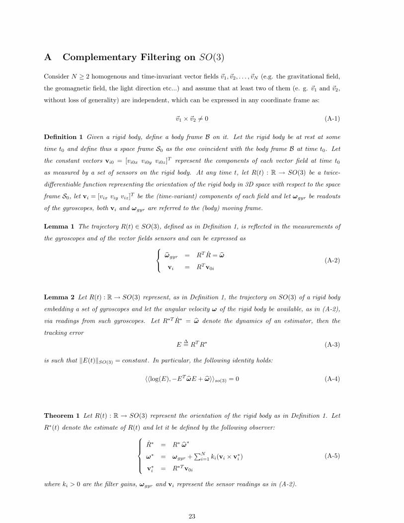
A Complementary Filtering on SO(3)

Consider N ≥ 2 homogenous and time-invariant vector fields ~v1, ~v2, . . . , ~vN (e.g. the gravitational field,

the geomagnetic field, the light direction etc...) and assume that at least two of them (e. g. ~v1 and ~v2,

without loss of generality) are independent, which can be expressed in any coordinate frame as:

~v1 × ~v2 6= 0 (A-1)

Definition 1 Given a rigid body, define a body frame B on it. Let the rigid body be at rest at some

time t0 and define thus a space frame S0 as the one coincident with the body frame B at time t0. Let

the constant vectors vi0 = [vi0x vi0y vi0z]T represent the components of each vector field at time t0

as measured by a set of sensors on the rigid body. At any time t, let R(t) : R → SO(3) be a twice-

differentiable function representing the orientation of the rigid body in 3D space with respect to the space

frame S0, let vi = [vix viy viz]T be the (time-variant) components of each field and let ωgyr be readouts

of the gyroscopes, both vi and ωgyr are referred to the (body) moving frame.

Lemma 1 The trajectory R(t) ∈ SO(3), defined as in Definition 1, is reflected in the measurements of

the gyroscopes and of the vector fields sensors and can be expressed as ωgyr = RT R = ω

vi = RTv0i

(A-2)

Lemma 2 Let R(t) : R→ SO(3) represent, as in Definition 1, the trajectory on SO(3) of a rigid body

embedding a set of gyroscopes and let the angular velocity ω of the rigid body be available, as in (A-2),

via readings from such gyroscopes. Let R∗T R∗ = ω denote the dynamics of an estimator, then the

tracking error

E∆= RTR∗ (A-3)

is such that ‖E(t)‖SO(3) = constant. In particular, the following identity holds:

〈〈log(E),−ET ωE + ω〉〉so(3) = 0 (A-4)

Theorem 1 Let R(t) : R → SO(3) represent the orientation of the rigid body as in Definition 1. Let

R∗(t) denote the estimate of R(t) and let it be defined by the following observer:R∗ = R∗ ω∗

ω∗ = ωgyr +∑Ni=1 ki(vi × v∗i )

v∗i = R∗Tv0i

(A-5)

where ki > 0 are the filter gains, ωgyr and vi represent the sensor readings as in (A-2).

23

The observer (A-5) asymptotically tracks R(t) for almost any initial condition R∗(0) 6= R(0) and in

particular:

limt→∞

RT (t)R∗(t) = I (A-6)

24

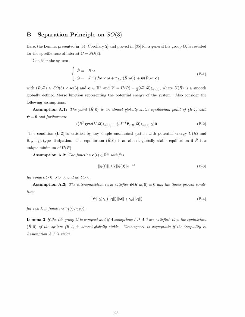
B Separation Principle on SO(3)

Here, the Lemma presented in [34, Corollary 2] and proved in [35] for a general Lie group G, is restated

for the specific case of interest G = SO(3).

Consider the system R = Rω

ω = J−1(Jω × ω + τFB(R,ω)) +ψ(R,ω,q)(B-1)

with (R, ω) ∈ SO(3) × so(3) and q ∈ Rn and V = U(R) + 12 〈〈ω, ω〉〉so(3), where U(R) is a smooth

globally defined Morse function representing the potential energy of the system. Also consider the

following assumptions.

Assumption A.1: The point (R, 0) is an almost globally stable equilibrium point of (B-1) with

ψ ≡ 0 and furthermore

〈〈RT gradU, ω〉〉so(3) + 〈〈J−1τFB , ω〉〉so(3) ≤ 0 (B-2)

The condition (B-2) is satisfied by any simple mechanical system with potential energy U(R) and

Rayleigh-type dissipation. The equilibrium (R, 0) is an almost globally stable equilibrium if R is a

unique minimum of U(R).

Assumption A.2: The function q(t) ∈ Rn satisfies

‖q(t)‖ ≤ c‖q(0)‖e−λt (B-3)

for some c > 0, λ > 0, and all t > 0.

Assumption A.3: The interconnection term satisfies ψ(R,ω, 0) ≡ 0 and the linear growth condi-

tions

‖ψ‖ ≤ γ1(‖q‖) ‖ω‖+ γ2(‖q‖) (B-4)

for two K∞ functions γ1(·), γ2(·).

Lemma 3 If the Lie group G is compact and if Assumptions A.1-A.3 are satisfied, then the equilibrium

(R, 0) of the system (B-1) is almost-globally stable. Convergence is asymptotic if the inequality in

Assumption A.1 is strict.

25

REFERENCES

[1] R.S. Fearing, K.H. Chiang, M.H. Dickinson, D.L. Pick, M. Sitti, and J. Yan, Wing transmission

for a micromechanical flying insect, in Proc. of the IEEE International Conference on Robotics and

Automation (ICRA), San Francisco, vol. 2, pp. 1509 - 1516 (2000).

[2] M.H. Dickinson, F.O. Lehnmann, and S.S. Sane, Wing rotation and the aerodynamic basis of insect

flight, Science, 284 (5422):1954-1960 (1999).

[3] R.J. Wood, Design, fabrication, and analysis, of a 3DOF, 3cm flapping-wing MAV, in Proc. of the

IEEE/RSJ International Conference on Intelligent Robotics and Systems (IROS), San Diego, pp.

1576-1581 (2007).

[4] R.J. Wood, The first takeoff of a biologically-inspired at-scale robotic insect , in IEEE Trans. on

Robotics, Vol.24, No. 2, pp. 341-347 (2008).

[5] G.K. Taylor, Mechanics and aerodynamics of insect flight control, in Biological Review, Vol. 76,

No. 4, pp. 449-471 (2001).

[6] X. Deng and L. Schenato and W.C. Wu and S.S. Sastry, Flapping Flight for Biomimetic Robotic

Insects. Part I: System modeling, in IEEE Transactions on Robotics, Vol. 22, No. 4, pp. 789- 803

(2006).

[7] X. Deng and L. Schenato and S.S. Sastry, Flapping Flight for Biomimetic robotic Insects. Part II:

Flight Control Design, in IEEE Transactions on Robotics, Vol. 22, No. 4, pp. 789- 803 (2006).

[8] P. Vela, K. Morgansen, and J.W. Burdick, Trajectory stabilization for a planar carangiform fish,

in Proc of the IEEE International Conference on Robotics and Automation (ICRA), Washington

DC, vol.1, pp. 756-762 (2002).

[9] L. Schenato and W.C. Wu and S.S. Sastry, Attitude Control for a Micromechanical Flying Insect

Via Sensor Output Feedback, in IEEE Transactions on Robotics and Automation, Vol. 20, pp.

93-106 (2004).

[10] H. Rifai and N. Marchand and G. Poulin, Bounded attitude control of a biomimetic flapping robot,

in Proc. of the IEEE International Conf. on Robotics and Biomimetics (ROBIO), Sanya, pp. 1-6,

(2007).

[11] M. Epstein, S. Waydo, S.B. Fuller, W. Dickson, A. Straw, M.H. Dickinson, R.M. Murray, Bio-

logically Inspired Feedback Design for Drosophila Flight, in Proc. of the IEEE American Control

Conference (ACC), New York, pp. 3395-3401 (2007).

[12] V. I. Arnold, Mathematical Methods of Classical Mechanics, 2 nd ed., Springer-Verlag, New York

(1989).

26

[13] R. M. Murray, Z. Li, and S. S. Sastry, A Mathematical Introduction to Robotic Manipulation, CRC,

Boca Raton, FL (1994).

[14] T. Frankel, The Geometry of Physics: an Introduction, Cambridge University Press, Cambridge,

UK (1997).

[15] S. S. Sastry, Nonlinear Systems: Analysis, Stability and Control, Springer, New York (1999).

[16] F. Bullo and A. D. Lewis, Geometric Control of Mechanical Systems, Springer (2005).

[17] F. Bullo and R. F. Murray Proportional derivative (PD) Control on the Euclidean Group, Technical

report, California Institute of Technology, Anaheim, CA USA (1995).

[18] S.P. Sane, The aerodynamics of insect flight, in Journal of Experimental Biology, Vol. 206, pp.

4191-4208 (2003).

[19] J. Chahl, Bioinspired engineering of exploration systems: a horizon sensor/attitude reference system

based on the dragonfly ocelli for mars exploration applications, in Journal of Robotic Systems, Vol.

20, No. 1, pp. 35-42 (2003).

[20] R. Hengstenberg, Mechanosensory control of compensatory head roll during flight in the blowfly

Calliphora erythrocephala, in Journal of Comparative Physiology A - Sensory Neural & Behavioral

Physiology, Vol. 163, pp. 151-165 (1988).

[21] G. Nalbach, The halteres of the blowfly Calliphora: I. Kinematics and dynamics, in Journal of

Comparative Physiology A, Vol. 173, pp. 293-300 (1993).

[22] W. C. Wu, R. J. Wood and R. F. Fearing, Halteres for the Micromechanical Flying Insect, in Proc.

of IEEE Intl. Conf. on Robotics and Automation (ICRA), Washington DC, vol.1, pp. 60-65 (2002).

[23] Absoluteastronomy.com, http://www.absoluteastronomy.com/topics/Halteres

[24] M.H. Dickinson, Linear and nonlinear encoding properties of an identified mechanoreceptor on the

fly wing measured with mechanical noise stimuli, in Journal of Experimental Biology, Vol. 151, pp.

219-244 (1990).

[25] H. Schuppe and R. Hengstenberg, Optical properties of the ocelli of Calliphora erythrocephala and

their role in the dorsal light response, Journal of Comparative Biology A, Vol. 173, pp. 143-149

(1993).

[26] Boris Krylov, Ekaweeka.com, https://www.ekaweeka.com/1251/gallery/9028/?show=post comment

[27] W. Reichardt and M. Egelhaaf, Properties of individual movement detectors as derived from be-

havioural experiments on the visual system of the fly, in Biological Cybernetics, Vol. 58, No. 5, pp.

287-294 (1988).

27

[28] D. Lambrinos, H. Kobayashi, R. Pfeifer, M. Maris, T. Labhart, R. Wehner, Adaptive Behavior An

Autonomous Agent Navigating with a Polarized Light Compass, in Adaptive Behavior, Vol. 6, No.

1, pp. 131-161 (1997).

[29] E. Wajnberga and G. Cernicchiaroa and D. Acosta-Avalosb and L. J. El-Jaicka and D. M. S.

Esquivel, Induced remanent magnetization of social insects, in Journal of Magnetism and Magnetic

Materials, Vol. 226-230, pp. 2040-2041 (2001).

[30] W. C. Wu, L. Schenato, R. J. Wood and R. F. Fearing, Biomimetic sensor suite for flight control

of MFI: design and experimental results, in Proc. of IEEE Intl. Conf. on Robotics and Automation

(ICRA), Tsipei, Vol. 1, pp. 1146-1151 (2003).

[31] R. G. Brown and P. Y. C. Hwang, Introduction to random signals and applied Kalman filtering, J.

Wiley, New York (1992).

[32] F. Daum, Nonlinear Filters: Beyond the Kalman Filter, in IEEE A&E Systems Magazine, Vol.20,

No. 8 (2005).

[33] D. Campolo, L. Schenato, L. Pin, X. Deng, E. Guglielmelli, Attitude stabilization of biologically

inspired micromechanical flying insects. Part I: attitude estimation via multimodal sensor fusion,

to appear on Advanced Robotics (Special Issue on Biomimetic Robotics).

[34] D. H. S. Maithripala, J. M. Berg and W. P. Dayawansa, An intrinsic observer for a class of simple

mechanical systems on a lie group, in SIAM Journ. Control Optim., Vol. 44, No. 5, pp. 1691-1711

(2005).

[35] D. H. S. Maithripala, J. M. Berg, and W. P. Dayawansa, Almost-global tracking of simple mechan-

ical systems on a general class of lie groups”, in IEEE Trans. on Automatic Control, Vol. 51, No.

1 (2006).

[36] D. E. Koditschek, The application of total energy as a Lyapunov function for mechanical control

systems, in J. E. Marsden, P. S. Krishnaprasad & J. C. Simo (eds), Dynamics and Control of

Multibody Systems, Vol. 97, AMS, pp. 131-157 (1989).

[37] F. Bullo and R. M. Murray, Tracking for fully actuated mechanical systems: a geometric framework,

in Automatica, Vol. 35, No. 1, pp. 17-34 (1999).

28