Asymmetry of Tidal Plume Fronts in an Eastern Boundary Current Regime

Journal of Marine Systems 78 (2009) 442–459

Contents lists available at ScienceDirect

Journal of Marine Systems

j ourna l homepage: www.e lsev ie r.com/ locate / jmarsys

Asymmetry of Columbia River tidal plume fronts

David A. Jay a,⁎, Jiayi Pan a, Philip M. Orton b, Alexander R. Horner-Devine c

a Department of Civil and Environmental Engineering, Portland State University, PO Box 751, Portland, OR 97201, USAb Ocean and Climate Physics, Lamont Doherty Earth Observatory, Columbia University, 61 Route 9W, Palisades, NY 10964, USAc Department of Civil and Environmental Engineering, University of Washington, Box 352700, Seattle, WA 98195-2700, USA

⁎ Corresponding author. Tel.: +1 503 725 4247.E-mail addresses: [email protected] (D.A. Jay), panj

[email protected] (P.M. Orton), [email protected]

0924-7963/$ – see front matter © 2009 Elsevier B.V. Adoi:10.1016/j.jmarsys.2008.11.015

a b s t r a c t
a r t i c l e i n f o
Article history:
Columbia River tidal plume Received 9 October 2006Received in revised form 1 April 2008Accepted 12 November 2008Available online 14 February 2009
Keywords:PlumesFrontsInternal wavesTidal effectsCalifornia currentUpwelling

dynamics can be explained in terms of two asymmetries related to plume-frontdepth and internal wave generation. These asymmetries may be an important factor contributing to theobserved greater primary productivity and phytoplankton standing crop on the Washington shelf. The tidalplume (the most recent ebb outflow from the estuary) is initially supercritical with respect to the frontalinternal Froude number FR on strong ebbs. It is separated from the rotating plume bulge by a front, whoseproperties are very different under upwelling vs. downwelling conditions. Under summer upwelling conditions,tidal plume fronts are sharp andnarrow (b20–50mwide) on their upwind ornorthern side andmark a transitionfrom supercritical to subcritical flow for up to 12 h after high water. Such sharp fronts are a source of turbulentmixing, despite the strong stratification. Because the tidal plumemayoverlie newly upwelledwaters, these frontscanmixnutrients into the plume. Symmetrywould suggest that there should be a sharp front south of the estuarymouth under summer downwelling conditions. Instead, the downwelling tidal plume front is usually diffuse onits upstreamside.Mixing isweaker, and thewatermasses immediately beloware low innutrients. There is alsoanupwelling–downwelling asymmetry in internal wave generation. During upwelling and weak wind conditions,plume fronts often generate trains of non-linear internal waves as they transition from a supercritical to asubcritical state. Under downwelling conditions, internal wave release is less common and the waves are lessenergetic. Furthermore, regardless of wind conditions, solition formation almost always begins on the south sideof the plume so that the front “unzips” from south to north. This distinction is important, because these internalwaves contribute to vertical mixing in the plume bulge and transport low-salinity water across the tidal plumeinto the plume bulge.FR and plume depth are key parameters in distinguishing the upwelling and downwelling situations, and thesetwoasymmetries canbeexplained in termsof potential vorticity conservation. Thedivergenceof the tidal outflowafter it leaves the estuaryembeds relative vorticity in the emerging tidal plumewatermass. This vorticity controlsthe transition of the tidal plume front to a subcritical state and consequently the timing and location of internalwave generation by plume fronts.

© 2009 Elsevier B.V. All rights reserved.

1. Introduction

A buoyant river plume and its fronts interact stronglywith ambientalongshore flow, influencing thereby vertical mixing, the nutrientsupply to surface waters, and the transport of organisms and particles.These issues have been studied to date in several contexts (e.g., Chao,1988; Fong et al., 1997; O'Donnell et al., 1998; Garcia-Berdeal et al.,2002; Hickey et al., 2005). Here, we consider the interaction of theColumbia River plume with the California Current. This interaction isimportant because it supports high levels of primary production andmajor fisheries in the Pacific Northwest (Landry et al., 1989), andbecause freshwater inflow is vital to the supply of micronutrients to

@cecs.pdx.edu (J. Pan),ton.edu (A.R. Horner-Devine).

ll rights reserved.

the entire California Current upwelling regime (Lohan and Bruland,2006).

More specifically, this paper investigates the interaction of theColumbiaRiver tidalplume frontswith theCalifornia Currentupwelling/downwelling regime. For this purpose, we use synthetic aperture radar(SAR) andocean colordata, vessel data collected 2004–2006 by theRISE(River-Influences on Shelf Ecosystems) project, and a scaling analysis.The “tidal plume” is the water from the most recent ebb. This usagereflects the fact that outflow from the Columbia River is discontinuous,occurring as distinct, high-velocity ebb pulses. The interactions of tidalplume fronts with the upwelling regime are of particular interest,because up to 20% of total mixing between river and oceanwater occurswithin 100 m behind the tidal plume front, even though this is b2% oftotal plume area (Orton and Jay, 2005). Internal waves spawned at thefront cause additionalmixing (Nash andMoum, 2005) not considered inthe Orton and Jay estimate.

mailto:[email protected]




http://dx.doi.org/10.1016/j.jmarsys.2008.11.015

http://www.sciencedirect.com/science/journal/09247963

443D.A. Jay et al. / Journal of Marine Systems 78 (2009) 442–459

Discussion of the interaction of the tidal plume with the upwellingregime is conveniently framed in terms of the two asymmetriesbetween tidal plume fronts observed during upwelling vs. downwellingperiods. During summer upwelling periods, our observations show thatthe tidal plume fronts remain super-critical for many hours after theyleave the estuary entrance, particularly on their upwind, northern side.They are sharp and narrow (20–50mwide) and mark a transition fromsupercritical to sub-critical flow for up to 12 h after high water. Despitehigh stratification, these fronts and the internal waves they generaterepresent a source of vigorous turbulent mixing north of the estuarymouth. Symmetry would suggest that, under summer downwellingconditions, there should be a sharp front south (upwind) of the estuarymouth. In fact, tidal plume fronts under summer downwelling periodsare usually broad and diffuse even on their upstream side, because atransition from supercritical to subcritical conditions has alreadyoccurred close to the estuary mouth. Less mixing is accomplished, andthe water immediately below the plume consists of old plume andsurface waters, both low in nutrients.

Internal wave generation by plume fronts is also asymmetric.Supercritical plume fronts often generate trains of non-linear internalwaves (IW) as they transition to a subcritical state. SAR imagespresented herein show that internal wave formation occurs frequentlyunder upwelling or neutral conditions, and less frequently underdownwelling conditions. Moreover, IW formation begins on the southside of the tidal plume (regardless of wind forcing) andmoves along theplume front so that the front “unzips” (undergoes fission) from south tonorth. This implies that a frontal transition fromsupercritical to subcriticalconditions first occurs south of the estuary mouth, regardless of whetherthis is the upwind or downwind side of the plume. We show below thatboth of these asymmetries can be explained in terms of potential vorticityconservation.

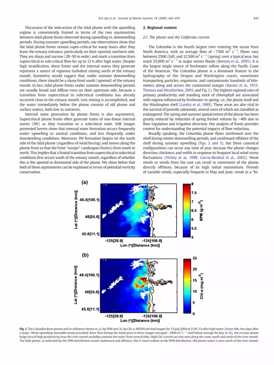
Fig. 1. The Columbia River plume and its influence shown in (a) by SPM and (b) by Chl-a;MODa neap). Weak upwelling-favorable winds prevailed. River flow during the week prior to thesbulge area of high productivity near the rivermouth probably contains thewater from severaThe bulk plume, as indicated by the SPM distribution trends southward and offshore; this is

2. Regional context

2.1. The plume and the California current

The Columbia is the fourth largest river entering the ocean fromNorth America, with an average flow of ~7300 m3 s−1. Flows varybetween 2500 (fall) and 12,500 m3 s−1 (spring) over a typical year, butreach 25,000 m3 s−1 in major winter floods (Bottom et al., 2005). It isthe largest single source of freshwater inflow along the Pacific Coastof the Americas. The Columbia plume is a dominant feature in thehydrography of the Oregon and Washington coasts, sometimestransporting particles, organisms, and contaminants hundreds of kilo-meters along and across the continental margin (Barnes et al., 1972;Thomas andWeatherbee, 2005, and Fig.1). The highest regional rates ofprimary productivity and standing stock of chlorophyll are associatedwith regions influenced by freshwater in spring; i.e., the plume itself andthe Washington shelf (Landry et al., 1989). These areas are also vital tothe survival of juvenile salmonids, several races of which are classified asendangered. The spring and summer spatial extent of theplumehas beengreatly reduced by reduction of spring freshet volume by N40% due toflow regulation and irrigation diversion. Our analysis of fronts providescontext for understanding the potential impacts of flow reduction.

Broadly speaking, the Columbia plume flows northward over theshelf duringwinter downwelling periods, and southward offshore of theshelf during summer upwelling (Figs. 2 and 3), but these canonicalconfigurations can occur any time of year, because the plume changesdirection, thickness and width in response to frequent local wind stressfluctuations (Hickey et al., 1998; Garcia-Berdeal et al., 2002). Weakwinds or winds from the east can result in movement of the plumedirectly offshore, because of its high initial momentum. Periodsof variable winds, especially frequent in May and June, result in a “bi-

IS derived images for 12 July 2004 at 2130, 5 h after highwater (lesser ebb, twodays aftere images averaged ~5000 m3 s−1, well below average for July. In (b), the circular plumel ebbs. High Chl-a levels are also seen along the coast, north and south of the rivermouth.most evident in the SPM distribution. Old plume water is seen north of the river mouth.

Fig. 2. Transition to upwelling: maps obtained 29 May to 3 June 2005 of salinity (a) and Chl-a (b) ~3 m below free surface during RISE-2; data are from the R/V Pt. Sur UDAS. Plumewaters have moved southwestward under the influence of weak upwelling-favorable winds, but old plume waters remain at the surface along the coast except at the very south endof the map. The large volume of freshwater input by the spring freshet caps upwelled waters along the coast; elevated Chl-a levels are seen only within the plume. Several stormsduring May caused nutrient levels in river water to be above average for the season.

444 D.A. Jay et al. / Journal of Marine Systems 78 (2009) 442–459

directional” plume with freshwater north and south of the river mouth(Hickeyet al., 2005). Because of theveryhighbuoyancy input, theplumenear-field and bulge are very stratified, with the 3–10 m thick plumeoverlying shelf waters. In the parlance of Yankovsky and Chapman(1997), theColumbia plume is in the “surface-advected” category, due tothe relatively narrow, steep shelf off the rivermouth. It differs, therefore,from the more-studied Rhine plume, which usually has a lowerbuoyancy input and stronger tides, allowing mixing to sometimesextend to the bed (e.g., Souza and Simpson,1997). The Columbia plumeaffects the bed only immediately beneath plume fronts and in the plumenear-field (Orton and Jay, 2005; Spahn et al., submitted for publication).

RISE observations show that there are several reasons why theColumbia plume is itself highly productive and contributes to regionalprimary production:

• The paradoxical nature of plume mixing: Despite high stratification,plume fronts exhibit vigorous mixing and disturb the seabed downto at least 50–60m (Orton and Jay, 2005). This contributes tomixingupwelled nutrients and iron (Fe) from re-suspended river sedi-ments into the surface layer.

• Plume nutrients and micronutrients: The plume supplies nitrogen(N), phosphate (P), iron (Fe) and manganese (Mn) from land (Jayet al., 2002; Lohan and Bruland, 2006).

• Compensating production: Elevated riverine nutrient input to theplume due to precipitation over the coastal subbasin of theColumbia River partially compensates for primary production lostduring periods of prolonged downwelling. This mechanism is mostimportant during years like 2005 when strong upwelling is delayeduntil midsummer (cf. Fig. 2).

An important feature of the Pacific Northwest coastal ecosystem isthat the standing stocks of chlorophyll and primary productivity areboth higher on the Washington shelf than the Oregon shelf (Landryet al., 1989; Hickey, 1989). The fact that the movement of new plumewater is often northward and onshore in a coastal current duringdownwelling vs. off-shelf and southward during upwelling is onefactor that may explain this observation. The northward movement ofFe-rich silt during winter storms is another important factor. Wesuggest in Section 5 that differences between upwelling and down-welling tidal plume fronts are also important. Upwelling fronts exhibit

Fig. 3. Moderate downwelling winds: a map obtained 18–20 June 2005 of salinity (a) and Chl-a (b) ~3 m below free surface during RISE-2; data are from the R/V Pt. Sur UDAS. Lowsalinity, new plumewater is found only in the near-field and north of the river mouth, though old plumewater is found to the south. Downwelling-favorable winds reached 10m s−1

on 17 June, but winds dropped to light and variable by the end of the survey period.


stronger mixing, and are more likely to mix plume and recentlyupwelled waters; this mixing occurs primarily north of the estuarymouth. Thus, frontal propagation provides a mechanism for mixing onthe shelf and slope in the sense of Kelvinwave propagation (northward)relative to the estuary mouth, where it would otherwise be suppressedby the stratification of the plume.

2.2. Plume anatomy and function

Understanding plume processes requires terminology for plumefunctional components. Garvine (1982) divided a steady buoyant plumeinto three zones or regimes: a source zone, the near-field and the far-field. The Columbia plume, where a very strong tidal outflow overridesand interacts with a larger anticyclonic plume bulge, requires adistinction between the tidal plume and the remainder of the plume

near-field. Thus, the Columbia plume has the following components(Fig. 3 in Horner-Devine et al., 2009-this volume):

• The plume source zone: The plume source zone is the area at theentrance of the estuary where low-salinity estuarine water lifts offfrom the seabed to form the nascent plume. Plume lift-off occurs atan internal hydraulic control (a width constriction associated withlateral stone jetty), near the landward boundary of the source zone(Cudaback and Jay, 1996, 2000). After lift-off, the plume flow islaterally confined by stone jetties for about 3 km before its expansioninto the coastal ocean as a tidal plume. An internal hydraulic control isa common feature of plume lift-off in river estuaries (e.g., in the FraserRiver, Macdonald and Geyer, 2004).

• The tidal plume: The tidal plume consists of the most recent ebboutflow fromtheplumeand is surroundedby strong fronts (Orton andJay, 2005; Nash andMoum, 2005). It remains distinct from the plume


bulge until its fronts become subcritical, after which time it graduallymerges into the rotating plume bulge. Under weak wind forcingconditions, the plume is semicircular to circular. Typical tidal plumediameters are 10–35 km. The scaling of the tidal-plume and plumebulge is considered in Horner-Devine et al. (2009-this volume).

• The plume bulge: The bulge surrounds the tidal plume under mostwind conditions (but may be displaced and diminished in size duringperiods of strong winds from the south). It usually contains the waterfromseveral ebbs and is separated from theplume far-field byadiffusefrontal zone.

• The plume far-field: The far-field is the zone beyond the bulgewherefinal mixing of plume and ambient seawater occurs; S=32 to 32.5defines its outer boundary (Barnes et al., 1972).

In addition to these four components, we also refer to the plume asa whole as the “bulk plume.”

These four zones provide a good basis for a detailed description ofthe features of Columbia tidal plume fronts and the internal wavesgenerated at these fronts. It is also useful to define a “front.” A front isa distinct boundary between two water masses. Tidal plume frontsoccur through convergence in the presence of a buoyancy gradientimposed by river inflow. A convergent front, especially one that issuper-critical, will have a well defined “head” or plunge at the visiblesurface signature, followed by a broader area of elevated mixing(O'Donnell et al., 2008).

3. Methods: data collection and processing

Sampling the Columbia River plume is challenging, because it isshallow (2–10 m) and highly mobile. It also varies on time scales ofless than a day and is characterized by length scales that are difficultto cover synoptically with a single vessel (Hickey et al., 1998). Therefore,

Fig. 4. 300 kHz ADCP current meter and wind times series for July 2004 for the central RISEpassed to remove tides; wind data have been filtered to remove diurnal sea breeze effects. Froall in m s−1. Time on the x-axis is in calendar days, July 2004 (PST). See (Fig. 6b) for moori

remote sensing data and results from towed vehicle (TRIAXUS) samplingare used herein. Despite the ~3 m s−1 tow speed of TRIAXUS, it wasnecessary to alternatebetween twosamplingmodes: a)plumescalemapsof 2–3 d duration, and b) process studies in a limited area, with 2–6 hrepeat times.

RISE physical oceanography was carried out on R/V Pt Sur. The R/VPt Sur performed rapid surveys using a towed body (the TRIAXUS,steerable in 3D) and the vessel's near-surface underway data acquisitionsystem or UDAS (nominally at 3 m depth). The high mobility ofTRIAXUS was used to sample surface waters (up to within 0.5–2 m ofthe surface, depending on sea state) outside of the ship wake. TRIAXUSwas used during three cruises. RISE1 (July 2004) occurred during aperiod of decreasing river flow after a weak spring freshet; prolongedupwellingwas seen at the end of the cruise. RISE2 (June 2005) occurredduring decreasing river flowafter aweak spring freshet; strong upwellingwas absent. RISE4 (June 2006) had moderately high but decreasing riverflow; some weak upwelling was observed.

Instrumentation was as follows. The R/V Pt Sur carried a pole-mounted acoustic Doppler current profiler (ADCP; 300 kHz for RISE1,1200 kHz for RISE2 and RISE4). The UDAS acquired position,meteorological data, salinity (S), temperature (T), and fluorescence at3 m. TRIAXUS carried a 911 SeaBird conductivity–temperature–depth(CTD) profiler equipped with sensors for nitrate (N), C, T, pressure,transmissivity and fluorescence, and other instruments not relevanthere. CTD casts were made at the beginning and end of maps with asecond, identical SeaBird 911 CTD for calibration purposes. The vesseland pole-mounted ADCP data sets and TRIAXUS scalar data are used inthe analyses described herein.

Synthetic aperture radar (SAR) and ocean color images are used inthis study to provide synoptic coverage of the plume area. SAR imageswere obtained from RADARSAT-1. The SAR data were archived anddistributed through the Comprehensive Large Array-data Stewardship

mooring at 46 10.02° N 124 11.72° W, in 69 mwater depth. Current data have been low-m top to bottom: wind, currents at 1.5 m, currents at 25m, and depth averaged velocity,ng locations.

Fig. 5.Well-established upwelling: a map obtained 24–27 July 2004 of salinity (a) and Chl-a (b) at ~2 m depth during RISE-1. Data are from the R/V Pt UDAS; tides were weak. Plumewaters have moved southward under the influence of sustained upwelling favorable winds. Upwelled waters are seen shoreward of the plume. MODIS-derived Chl-a (c) for 23 July2004 at 2110 UT, ~8 h after high water (neap tide); Chl-a standing stock is generally low and mostly associated with plume waters.


System (CLASS) of National Oceanic and Atmospheric Administration(NOAA). Here, our use of the images involves rectification and editingto include only the relevant region near the mouth of the Columbia.

The ocean color data used here are from the Moderate ResolutionImaging Spectro-radiometer (MODIS) aboard an Aqua satellite,launched on 4 May 2002. Aqua MODIS views the entire Earth's

surface every 1 to 2 days, acquiring data in 36 spectral bands. TheMODIS ocean color data have been processed using O'Reilly et al.(1998) for chlorophyll a (Chl-a) and Van Mol and Ruddick (2005) forsuspended particulate matter (SPM). To obtain concentrations of Chla and suspended particulate matter (SPM), we used the normalizedwater leaving radiance (nLw) at bands of 412 nm, 443 nm, 488 nm,


531 nm, and 551 nm. The nLw data are available from: http://oceancolor.gsfc.nasa.gov.

4. Results: plume front dynamics

The asymmetries in frontal strength and internal wave generationdefined in the introduction are a multi-scale problem, both concep-tually and logistically, because the tidal plume (with its fronts andinternal waves) is embedded within the plume near-field and themuch larger plume far-field. The analysis in this section moves,therefore, from bulk-plume scales (described by remote sensing andvessel survey maps), to the tidal plume (described primarily by SARimages), to the tidal plume fronts and internal waves (described bySAR images and TRIAXUS sections). Regional context is provided bymoored instrument data (Fig. 4). A dynamical explanation for theasymmetries described in this section is provided in the Discussion(Section 5).

4.1. Summer plume configurations

We begin by defining bulk plume configurations. The size andposition of the bulk plume is related to the amount of Columbia River

Fig. 6. SAR images for (a) upwelling (26 July 2004 at 1439 UT, 8 h after highwater; a greater ebhigh water, a neap tide). Also shown for both cases is the hypothetical vorticity incurred by thsolitons visible on the west side of the plume. In (b) the upwind, S-SW quadrant of the tidaoutside the tidal plume, appear to have originated in deep water and are propagating landwatwo mooring sites are shown by +. A typical strong soliton pattern (c) and a typical weak

outflow, ambient currents, and coastal winds. There are four plumeconfigurations that occur frequently during spring and summer inresponse to variable forcing (Hickey et al., 2005): upwelling (Figs. 2,5a and b and 6a), weak and variable winds (with a tidal plume similarto that for upwelling winds; Fig. 1), downwelling (Figs. 3 and 6b), andbi-directional (combining features of Figs. 2 and 3). See Fig. 3 ofHorner-Devine et al. (2009-this volume) for a conceptual view ofplume configurations. Note that in terms of atmospheric forcing, thereare only three states (upwelling-favorable, weak or neutral winds, anddownwelling favorable). The bi-directional plume is a result ofvariable wind forcing over time, often after a period of elevated flow.

A typical example of summer winds and currents observed at amooring in the plume area is shown in Fig. 4 for July 2004 (see Fig. 6afor mooring location). Light and variable winds (b5 m s−1) prevaileduntil 17 July. This was followed by a brief downwelling episode 18–20July with winds to 6 m s−1, then persistent upwelling favorable windsas strong as 7 m s−1 on 21 July. While there is only a small disparity inthe magnitude of the upwelling vs. downwelling-favorable winds,there is a much stronger difference in the currents at 1.5 m depth.Southward near-surface currents exceed 0.4 m s−1 on two occasions,while northward currents never reach 0.2 m s−1. This disparity occursonly at the surface — at 25 m, currents are predominantly northward,

bwithmoderate tidal range) and (b) downwelling (24May 2003 at 1439 UT, ~10 h aftere upwind plume front in each case (see discussion in Section 5.1). In (a), there are 10–12l plume front has dissipated. Internal waves south of the river mouth, both inside andrd. The location of the 2005 RISE mooring data in Fig. 4 is shown by an x in (b); the othersoliton pattern (d).

http://oceancolor.gsfc.nasa.gov

http://oceancolor.gsfc.nasa.gov


while depth-averaged currents show little predominance. The moor-ing shown in Fig. 4 is most representative of conditions in the plumenear-field, but the other two RISE moorings show a similar (or larger)predominance of surface flow to the south; their locations are alsoshown in Fig. 6b.

Though there are four common summer bulk plume configurationsand three forcing conditions, we focus here on upwelling and

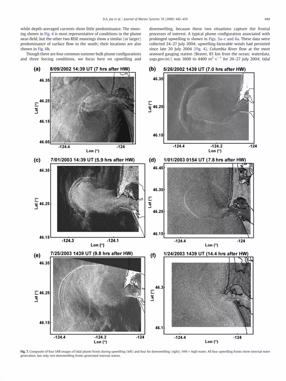
Fig. 7. Composite of four SAR images of tidal plume fronts during upwelling (left) and four fogeneration, but only two downwelling fronts generated internal waves.

downwelling, because these two situations capture the frontalprocesses of interest. A typical plume configuration associated withprolonged upwelling is shown in Figs. 5a–c and 6a. These data werecollected 24–27 July 2004; upwelling-favorable winds had persistedsince late 20 July 2004 (Fig. 4). Columbia River flow at the mostseaward gauging station (Beaver, 85 km from the ocean; waterdata.usgs.gov/or/) was 3600 to 4400 m3 s−1 for 20–27 July 2004; tidal

r downwelling (right); HW=high water. All four upwelling fronts show internal wave

Fig. 7 (continued).

Table 1Summary for 2001–2003 of fronts observed in SAR images, by forcing condition.

Wind direction Stronga Weakw/ IWb

Strong+weakwith IW

Weakc Grandtotal

Upwelling(52 cases)

N&NW 8 14 22 8 30S&SW 4 0 4 2 6Both 3 1 4 2 6Total/% 15/29 15/29 30/58 12/23 42/81

Neutral(43 cases)


Downwelling(34 cases)


All forcingconditions(132 cases)


a Strong: there is a narrow band of intense reflection.b Weak with IW: a front is weak, but front-generated, seaward propagating internal

waves appear.c Weak: a front is visible but faint or diffuse.


forcing was weak, 50–60% of the long-term average of 7300 m3 s−1.The UDAS data in Fig. 5a show the plume moving southward and offthe slope with Sb31 water as far south as 45.3° N. Newly upwelledwater (SN33.5) reaches the surface inshore of the new plume south of46° N. High Chl-a levels are seen along the outer edge of the newplume to the north of the entrance and as its spreads offshore between45.95° N and 46.2° N, and at the inshore end of several lines.

A MODIS-derived Chl-a map for 23 July 2004 shows high Chl-alevels (up to ~25mgm−3) and suggests strong productivity inshore ofthe plume, where some mixing of plume and upwelled water hasoccurred (Fig. 5c). There are also elevated Chl-a levels in a bandextending offshore through the plume at about 45.85° N. A similarmap for 22 July 2004, just after the onset of upwelling, suggests strongproductivity around the margins of the plume, especially on its southside. Such Chl-a is likely the result of productivity associated withwind mixing of upwelled water into the plume as the plume bulgethinned and spread south into an area not occupied by the bulge theprevious day (cf. Fong and Geyer, 2001). This interpretation issupported by a broad band of T=12–14 °C water on the 22 July2004 SST map that corresponds to the higher Chl-a; new tidal plumewaters had T=15–17 °C at this time (not shown).

The MODIS image does not define the tidal plume configuration,but Fig. 6a, a SAR image taken 26 July 2004, shows the correspondingtidal plume configuration. Note the strong tidal-plume front on thenorth side of the plume, where the plume is propagating into theoncoming flow, and internal wave generation has not yet taken place.There are at least six internal waves generated from a fission pointthat, given the propagation distances of the internal waves, has movedfrom south to north. These conditions are typical for upwelling.

Salinity and Chl-a for a typical bulk-plume configuration associatedwith downwelling are shown in Fig. 3. These observations werecollected 18–20 June 2005 just before a spring tide and two days aftera transition to downwelling favorable winds on 16 June 2004. Windswere weak and variable by the end of the map. River flow averaged6400 m3 s−1 and was decreasing slowly after the peak of the springfreshet on 20 May 2004 (~10,000 m3 s−1). The lowest salinity waterassociated with the tidal plumewater is directly offshore of themouthat 45.25° N; new plumewater has also moved northward between the50 and 100 m isobaths. Moderate levels of Chl-a are associated withthe plume bulge, north of the river mouth, but little Chl-a is beingproduced along the coast. The year 2005 was notable for the absenceof sustained upwelling before mid-July. Under those conditions, theriver and plume provides a significant part of the total (muchreduced) production of Chl-a in the plume region. We do not have aSAR images for this time period, but a SAR image for similar springflow levels in 2003 (Fig. 6b) shows a weaker front without internal

wave generation. In fact, the front has dissipated entirely on its south(upwind) side. These conditions are typical for downwelling.

4.2. Occurrence of fronts and internal waves relative to forcing

Now consider tidal plume configurations for upwelling anddownwelling in the context of the asymmetries mentioned in theIntroduction. Fig. 7 includes eight representative SAR images (fourupwelling and four downwelling) that show tidal plume fronts and/or plume-front generated internal waves. Fig. 7 conveys the idea thatfronts are stronger under upwelling than downwelling conditions.Table 1 tabulates frontal properties in 52 SAR images for the 2001–2003 period for upwelling (winds predominantly to the south), 43for neutral (winds not predominantly alongshore) conditions, and34 for downwelling (winds predominantly to the north) conditions.Interestingly, Table 1 shows that it is primarily when the occurrenceof weak fronts with internal waves is added to the occurrence ofstrong fronts that a difference between upwelling (and neutral)conditions is seen relative to downwelling conditions. The rationalefor summing these two situations is as follows. Internal wavegeneration can remove as much as 75% of the total energy of a front(Pan and Jay, 2008), greatly reducing it advance speed into ambientwater. We infer, therefore, that fronts that have released internal

Table 2Summary for 2001–2003 of plume-front generated internal waves in SAR images,classified by wind forcing condition.

Cases Stronga number/% Weakb number/% Total number/%

Upwelling (52 cases) 9/17 6/12 15/29Neutral (43 cases) 4/9 7/16 11/26Downwelling (34 cases) 2/5 5/11 7/16

a A SAR image is classified as having “Strong” internal waves when there is a clear,obvious internal wave pattern.

b A classification of “Weak” indicates that the internal wave pattern is faint or barelyvisible. Typical strong and weak solitons displayed in Fig. 6c and d.


waves were strong until their transition to subcritical condition andrelease of the waves. On this basis, upwelling and neutral conditionsdo more commonly show strong (or recently strong) fronts, but thedifference is not huge.

There is a larger difference, however, in internal wave generationcharacteristics. Table 2 summarizes internal wave occurrence byforcing condition. (Fig. 6c and d show “Strong” and “Weak” internalwaves, as used for classification in Table 2.) SAR images taken duringupwelling and neutral conditions more commonly show front-generated internal waves (especially strong internal waves) than dodownwelling images. In fact, only two downwelling cases show stronginternal wave generation. This is important, because the rate ofconvergence at a front or internal wave “crest” is directly related to thestrength of the SAR scattering cross-section — a stronger backscatterindicates a more energetic wave or front (Pan et al., 2007). Also, wheninternal wave generation is occurring, SAR images show a “fissionpoint” — the location at which an internal wave is just leaving theplume front (cf. Fig. 6a). As further discussed in Section 4.6, the fissionpoint always moves from south to north, un-zipping the front to

Fig. 8. Section showing internal wave fission from an upwelling plume front on 13 June 200tide). Shown are: a) salinity, (b) cross-frontal velocity in m s−1 from the 1200 kHz ADCP, wThe disturbance due to the front and internal wave penetrates to the bottom of the ADCPestimation of frontal and ambient (upstream) conditions.

produce non-linear internal waves. South-to-north fission is char-acteristic for all the internal waves captured in Fig. 7 and for almost allthe SAR images summarized in Table 2, regardless of the sense ofcoastal forcing (upwelling, neutral or downwelling).

4.3. Upwelling frontal phenomenology and processes

We now examine the details of plume frontal propagation andinternal wave generation by the tidal plume fronts, first for upwelling,then for downwelling. TRIAXUS sections taken on a neap tide, 13 June2005, are typical for upwelling and neutral conditions (Figs. 8 and 9).The TRIAXUS section in Fig. 8 captures the initial fission of anorthwestern front, ~5.6 h after high water. Fig. 9 shows a detail ofa later stage of evolution of the internal wave train, starting 8 h afterhigh water. A partial MODIS map for 13 June 2005 shows that thelarge-scale picture was similar to that shown in Fig. 2 for 29 May to 3June 2005. The light northwesterly (upwelling-favorable) winds thatbegan on 12 June 2005 were sufficient, in any event, to cause tidalplume fronts to behave in the manner similar to Fig. 6a. The priorweek's river flow averaged 6800 m3 s−1, down from a freshet peak on20May 2005 of 10,200m3 s−1 and 3000m3 s−1 below season averagefor mid-June.

The double depression in Fig. 8 represents a front (to the right at124.314° W) and a newly spawned internal wave left of the front (at124.318° W). The front, on the northwest side of the tidal plume, ispropagating at 0.54 m s−1 into a relatively stratified plume bulge(Fig. 8b). High salinity, upwelled waters are found below 25–30 m.The front has become subcritical (FR=0.4) and has slowed afterinternal wave release. (Here, FR=Uf / (g′Ha)1/2 is the frontal FRnumber, Uf is frontal speed, estimated by the velocity of plumewater above a near surface stability maximum and relative to the

5 1638 to 1941 UT; frontal crossing occurred at ~1810 UT, ~5.6 h after high water (neapith estimated internal FR number, and (c) ADCP echo intensity corrected for absorption.section at 25 m; salinity is perturbed to 35 m. Vertical lines define regions used for

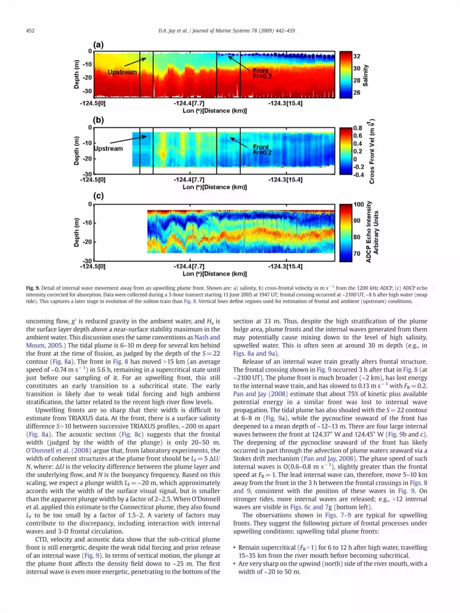
Fig. 9. Detail of internal wave movement away from an upwelling plume front. Shown are: a) salinity, b) cross-frontal velocity in m s−1 from the 1200 kHz ADCP, (c) ADCP echointensity corrected for absorption. Data were collected during a 3-hour transect starting 13 June 2005 at 1947 UT; frontal crossing occurred at ~2100 UT, ~8 h after high water (neaptide). This captures a later stage in evolution of the soliton train than Fig. 8. Vertical lines define regions used for estimation of frontal and ambient (upstream) conditions.


oncoming flow, g′ is reduced gravity in the ambient water, and Ha isthe surface layer depth above a near-surface stability maximum in theambient water. This discussion uses the same conventions as Nash andMoum, 2005.) The tidal plume is 6–10 m deep for several km behindthe front at the time of fission, as judged by the depth of the S=22contour (Fig. 8a). The front in Fig. 8 has moved N15 km (an averagespeed of ~0.74 m s−1) in 5.6 h, remaining in a supercritical state untiljust before our sampling of it. For an upwelling front, this stillconstitutes an early transition to a subcritical state. The earlytransition is likely due to weak tidal forcing and high ambientstratification, the latter related to the recent high river flow levels.

Upwelling fronts are so sharp that their width is difficult toestimate from TRIAXUS data. At the front, there is a surface salinitydifference SN10 between successive TRIAXUS profiles, ~200 m apart(Fig. 8a). The acoustic section (Fig. 8c) suggests that the frontalwidth (judged by the width of the plunge) is only 20–50 m.O'Donnell et al. (2008) argue that, from laboratory experiments, thewidth of coherent structures at the plume front should be LF=5 ΔU/N, where: ΔU is the velocity difference between the plume layer andthe underlying flow, and N is the buoyancy frequency. Based on thisscaling, we expect a plunge width LF=~20 m, which approximatelyaccords with the width of the surface visual signal, but is smallerthan the apparent plunge width by a factor of 2–2.5. When O'Donnellet al. applied this estimate to the Connecticut plume, they also foundLF to be too small by a factor of 1.5–2. A variety of factors maycontribute to the discrepancy, including interaction with internalwaves and 3-D frontal circulation.

CTD, velocity and acoustic data show that the sub-critical plumefront is still energetic, despite the weak tidal forcing and prior releaseof an internal wave (Fig. 9). In terms of vertical motion, the plunge atthe plume front affects the density field down to ~25 m. The firstinternal wave is evenmore energetic, penetrating to the bottom of the

section at 33 m. Thus, despite the high stratification of the plumebulge area, plume fronts and the internal waves generated from themmay potentially cause mixing down to the level of high salinity,upwelled water. This is often seen at around 30 m depth (e.g., inFigs. 8a and 9a).

Release of an internal wave train greatly alters frontal structure.The frontal crossing shown in Fig. 9 occurred 3 h after that in Fig. 8 (at~2100 UT). The plume front is much broader (~2 km), has lost energyto the internal wave train, and has slowed to 0.13 m s−1 with FR=0.2.Pan and Jay (2008) estimate that about 75% of kinetic plus availablepotential energy in a similar front was lost to internal wavepropagation. The tidal plume has also shoaled with the S=22 contourat 6–8 m (Fig. 9a), while the pycnocline seaward of the front hasdeepened to a mean depth of ~12–13 m. There are four large internalwaves between the front at 124.37° W and 124.45° W (Fig. 9b and c).The deepening of the pycnocline seaward of the front has likelyoccurred in part through the advection of plume waters seaward via aStokes drift mechanism (Pan and Jay, 2008). The phase speed of suchinternal waves is O(0.6–0.8 m s−1), slightly greater than the frontalspeed at FR=1. The lead internal wave can, therefore, move 5–10 kmaway from the front in the 3 h between the frontal crossings in Figs. 8and 9, consistent with the position of these waves in Fig. 9. Onstronger tides, more internal waves are released; e.g., N12 internalwaves are visible in Figs. 6c and 7g (bottom left).

The observations shown in Figs. 7–9 are typical for upwellingfronts. They suggest the following picture of frontal processes underupwelling conditions; upwelling tidal plume fronts:

• Remain supercritical (FRN1) for 6 to 12 h after high water, travelling15–35 km from the river mouth before becoming subcritical.

• Are very sharp on the upwind (north) side of the rivermouth, with awidth of ~20 to 50 m.

Fig. 11. Downwelling conditions: a TRIAXUS section corresponding to the first, more landward transect in Fig. 10; data were collected 19 July 2004, 4–5 h after high water (2 d after aspring tide). Shown are: (a) TRIAXUS salinity, and (b) across-frontal velocity as a function of depth, with the frontal Froude number FR. FR is calculated for the front relative toupstream conditions using the zones shown in (b). The entire frontal zone is wider than for upwelling, extending from ~46.166 to 46.172° N, N300 m.

Fig.10. SAR image taken 19 July 2004 at 1428 UT, about 5.5 h after high water under downwelling conditions (2 d after a spring tide), simultaneous with a TRIAXUS section. The Pt SurUDAS salinity data overlaid on the SAR image were collected between 1322 and 1511 UT. The southern front is diffuse and deeper than upwelling fronts. There has been a transitionbetween the time of the two transects from supercritical to subcritical conditions.



• Bound a tidal plume that is shallower on its upwind side than duringdownwelling, are more energetic, and can accomplish more mixingthan downwelling fronts (cf. Section 4.5).

• Are underlain by upwelled water (high in the nutrients, N and P) andsurface ocean water. Thus, they should contribute to primary produc-tion more effectively than downwelling fronts, which overlie surface-ocean or old plume waters, both of which are nutrient depleted.

• Frequently spawn, upon transition to subcritical conditions, anenergetic internal wave train that may contribute to mixing outsidethe plume and carries tidal plume water across the front (Pan et al.,2007).

An interpretation of these phenomena in terms of vorticityconservation is provided below.

4.4. Downwelling frontal phenomenology and processes

The observations used to describe typical summer downwellingfrontal phenomena stem from 19 July 2004; a regional salinity map isshown in Fig. 3. This downwelling episodewas brief (17–20 July), withpeak polewardwinds on 18 July of ~6m s−1. Fig.10 shows a SAR imagefor 19 July 2004 at 1428 UT, 2 d after a spring tide. Superimposed onthe SAR image are two 3 m salinity traces (from the R/V Pt Sur UDAS)across the frontal zone, covering the time period from 1322 to 1511 UT,~4 to 6 h after high water. A moderately sharp front is seen at ~46.17°N in the earlier (more landward) of the two transects, but the secondcrossing of the frontal zone (covering the time of the SAR image)shows a diffuse frontal zone at ~46.2° N. Thus, a transition fromsupercritical to subcritical conditions has occurred between the timesof the two transects. No seaward propagating internal waves weregenerated in the southern sector by this front, as is clear from theabsence of such waves seaward of the front in Figs. 11 and 12. (There

Fig.12.Downwelling conditions: a TRIAXUS section corresponding to the second, more seawaspring tide). Shown are: (a) TRIAXUS salinity, and (b) across-frontal velocity as a functioncritical conditions has occurred between the two sections. FR is calculated for the front relativextending from ~46.167 to 46.2° N, N2 km.

are several bands behind themain front in Figs.10–12, and their originis unclear.)

The TRIAXUS sections corresponding to the surface traces in Fig. 10are shown in Figs. 11 and 12. The first section, the more landward ofthe two in Fig. 10, shows a well-defined front, ~300 mwide as judgedfrom the salinity transition zone (Fig. 11a). The front is propagating at0.59 m s−1 into nearly motionless (Fig. 11b), weakly stratified water.Total propagation distance over 4.5 h was ~15 km. There is a plungedefined by a single ADCP ensemble, which penetrates N30 m, deepenough to cause somemixing with high salinity, upwelled waters. Thefront is supercritical, with FR=~2. Between the times of Figs. 11 and12, the plume deepened and became just subcritical (FR=0.9); itsfront is more diffuse. Also, the base of the plume (judged by the S=31contour) is at 8–14 m at right, deeper than in the upwelling case(compare Figs. 8a and 9awith Figs.11a and 12a). After the transition tosubcritical, the frontal speed has slowed to 0.14 m s−1 (Fig. 12b). Afrontal plunge is barely visible in the ADCP record (Fig. 12b), affectingthe flow only to about 12 m. Even though this is a spring tide and thesections were occupied before the end of the ebb (4–6 h after highwater), the frontal zone is ~2 km wide (from ~46.167 to 46.2° N).

Clearly, the downwelling front in Figs. 10–12 is more diffuse thanthe upwelling front in Figs. 8 and 9. This situation is typical fordownwelling conditions — upwind fronts during downwelling makean early transition to subcritical, usually without releasing internalwaves. The absence of internal waves may be related to the lowambient stratification as well as to lower frontal energy levels. What isunusual about this pair of sections is that we were able to capturesupercritical condition at all. Normally the transition to subcriticalconditions occurs close to the estuary mouth, in an area too shallowfor TRIAXUS observations. It is likely that an atypically long period ofsupercritical propagation occurred because of the large tidal rangeprevailing at this time.

rd transect in Fig.10; datawere collected 19 July 2004, 5–6 h after high water (2 d after aof depth, with the frontal internal Froude number FR. A transition from critical to sub-e to upstream conditions using the zones shown in (b). The entire frontal zone is broad,


In summary, tidal plume fronts during summer downwellingconditions typically:

• Make an early transition to a subcritical state, b10–20 km from theestuary mouth, often before the end of ebb.

• Are, after transition, diffuse on the upwind (south) side, such that“frontal zone” is perhaps a better descriptor than “front”.

• Are deeper on the upwind side than upwelling fronts, and cause lessmixing (cf. Section 4.5).

• Usually do not spawn internal wave trains that contribute to mixingoutside the plume.

4.5. Upwelling vs. downwelling differences in mixing

One method to evaluate the relative strength of mixing on theupstream side for upwelling and downwelling plume fronts is toexamine plume layer properties for typical sections. Fig. 13 contrastsplume upper-layer depth H, upper-layer salinity S, and bulkRichardson number Rib = gΔρH

ΔU for the upwelling sections shown inFigs. 8 and 9 versus the downwelling sections in Figs. 11 and 12. (H isthe depth of water above a near-surface stability maximum, and Rib is

Fig. 13. A comparison of plume layer-averaged properties between upwelling and downwelliupwelling (c) and downwelling (d), bulk Richardson number Rib for upwelling (e) and downwfull section, Figs. 8 and 9 for upwelling and Figs. 11 and 12 for downwelling. The x-axis for (a)other details.

based on the velocity ΔU and density Δρ contrasts between the upperand lower plume layers.) Of the four sections, one occurs before(Fig. 11), and three after (Figs. 8, 9 and 12) the transition to subcritical.Especially in the section corresponding to Fig. 8 (just after thetransition to subcritical conditions), the layer depth is smaller for theupwelling case, though layer depths are rather irregular for thedownwelling case.

Only the section that corresponds to Fig. 8, for upwelling, shows aRib value at or belowcritical level for suppression ofmixing (~0.25) forany considerable distance, and then primarily on the plume side,where elevatedmixing is expected. This same section shows a gradualincrease in S over 4 km in a region where Rib is essentially critical,while H is actually decreasing in the direction of propagation. Thissuggests that plume spreading andmixing are both active, but that themixing is not rapid enough to counteract spreading. The secondupwelling section (for Fig. 9) shows an abrupt increase in S at thepoint of initial internal wave generation and then a gradual furtherincrease in S in the seaward direction; H shows a slight thinningseaward of the fission point. If mixing is occurring seaward of thefission point, it may be due to a combination of internal wave andmean shear not reflected in our Rib, which is based onmean shear. The

ng conditions: plume depth H for upwelling (a) and downwelling (b), salinity at 3 m forelling (f), and (g) transect locations. The numbers in (a) refer to the figure showing theto (f) is distance in km along the transect from the location of the “x” in (g). See text for


downwelling sections (for Figs. 11 and 12) show generally larger layerdepths, RibN5, a gradual increase in S across the front, and a nearlyconstant S behind the front.

These salinity changes and layer depths strongly suggest thatmore mixing is associated with upwelling plume than downwellingfronts, and that internal waves are responsible for mixing beyondthe plume front. The plume behind the downwelling fronts is alsodeeper. These features are consistent with potential vorticity controlof frontal dynamics and internal wave generation described belowin Section 5.1.

4.6. Asymmetry of internal wave generation

Sections 4.2–4.5 document tidal plume properties for variousplume forcing conditions. Here, we examine internal wave generationby tidal plume fronts. Table 2 categorizes tidal plume-generatedinternal waves in SAR images by forcing condition (upwelling, neutralor downwelling). Internal waves generated at the tidal plume front arevisible in 29% of the upwelling, 26% of the neutral cases, and 16% of thedownwelling cases. Strong internal waves are seen in 17, 9 and 5%(respectively) of the upwelling, neutral and downwelling cases,emphasizing the more energetic nature of upwelling fronts. Thispredominance of strong internal wave generation under upwellingand (to a lesser extent) neutral conditions is consistent with theargument in Section 4.5 that these fronts are responsible for moremixing.

Not only is generation of internal wave trains by downwellingplume fronts less common than for upwelling and neutral fronts, butthe direction of movement of the fission point does not changebetween upwelling and downwelling. In all upwelling and neutralcases and all downwelling cases for which the sense of frontal fissioncan be discerned, the front “unzips” from south to north. (There aretwo downwelling cases where the direction of unzipping is unclear,but that there are no confirmed examples for any forcing conditionwhere the internal waves unzip from north to south.) This south tonorth unzipping is seen, for example, in the four upwelling cases inFig. 7, as well as in the two downwelling cases with internal waves. Inboth of the downwelling cases, the front on the southerly side of thetidal plume has become indistinct by the end of ebb. The tidal plumefront has unzipped from the southern quadrant to the northwest side,and an internal wave train is seen along the west side of the tidalplume.

In summary, when internal waves are generated by tidal plumefronts, the front first became subcritical on the south side of the tidalplume, leading to “unzipping” of the front from south to north. Asargued in the next section, the most satisfactory explanation of thisasymmetric internal wave generation is that the vorticity embeddedin the emerging plume by the tidal outflow, not the strength anddirection of alongshore currents, primarily controls the timing andlocation of internal wave generation from fronts.

5. Discussion and conclusions

5.1. A dynamical interpretation of tidal plume behavior in terms ofpotential vorticity

Analysis of tidal-plume potential vorticity conservation can be usedto understand the asymmetric behavior of tidal plume fronts andinternal waves. Potential vorticity is useful because it explains temporalchanges in the frontal internal Froude number FR=Uf/(g′Ha)½ asso-ciated with the tidal plume, which governs internal wave generation.Consider conservation of potential vorticity Ω=( f+ξ)/H following aparcel ofwater (assumed vertically uniform) emerging from the estuarywith the tidal plume front; ξ=(∂v/∂x−∂u/∂y) is thevertical componentof vorticity, f is planetary vorticity, and H is plume layer depth. The tidalstream (the ebb jet) seaward of the estuary entrance and alongshore

coastal currents transfer vorticity to the nascent plume, altering itsvelocity and vorticity, and constraining the time and space variations ofH. The results are different, however, for summer upwelling anddownwelling situations.

Conservation of Ω and mass require for this emerging parcel ofplume water:

DXDt

=D f + n

H

� �

Dt= − 1

Hj ×

τ→i

Hρ0ð5:1Þ

jH � [H = − 1HDHDt

ð5:2Þ

Where: ∪H={u,v} is the plume horizontal velocity, τ→i is theinterfacial stress vector, ∇H={∂/∂x, ∂ /∂y}; x is onshore and y isalongshore, and ρ0 is reference density. Assume for the moment thatthe plume is inviscid (unaffected by mixing) but that it takes onvorticity from the underlying tidal and coastal flows while stillspreading radially due to its own buoyancy forcing. Changes in f overthe tidal plume are also neglected as small. These assumptions arejustified below using a scaling analysis, and effects of mixing areaddressed. Because the analysis is inviscid, this analysis cannot beused to describe the highly non-hydrostatic plume front itself, whererelatively strong mixing occurs. It is intended to apply to waters justbehind the front.

The initial mid-channel condition at the plume lift-off point(where the initial value of H is set) is that ξ0≅0 because: a) v=∂v/∂x~0 (the flow is straight west [with ub0] and axially non-divergentin a jetty-constrained channel of nearly constant width and depth),and b) ∂u/∂y=0 inmid-outflow because the tidal outflow is strongestin mid-channel. Once the plume has left the estuary, there is lateralshear in the jet-like ebb outflow (Chao, 1990). Specifically, ∂v/∂xb0and ∂u/∂yN0 north of the channel centerline (so that ξ decreases),while ∂v/∂xN0 and ∂u/∂yb0 south of the channel centerline (so that ξincreases).

Now consider near-frontal water parcels on the upwind side of theriver mouth for upwelling and downwelling conditions; see Fig. 6aand b for a conceptual view of plume potential vorticity:

• Upwelling: the winds are from north to south, and the upwind frontis to the north of the river mouth. The upwind front remainssupercritical (FRN1) for ~6–12 h after high water, with a sharp front(Section 4). For water in a northward turning plume front, thespreading and anticyclonic rotation of the tidal outflow causes ξ todecrease (ξbξ0; Fig. 6a). The scale of the tidal plume (b25 km) issmall enough that changes in f are small relative to those in ξ.Therefore, H must decrease to conserve Ω (Eq. (5.1)), maintainingrapid seaward movement of the front. From Eq. (5.2), the plumespreading necessary to decrease H can occur both by axial andlateral divergence. Given any fixed density contrast, the small H andhigh velocity will raise the frontal Froude number FR. The front stayssharp because waves cannot propagate away from it. Frontal energyis eventually lost by a pulse of internal wave generation (Nash andMoum, 2005), but this typically occurs after the end of ebb, well intothe following flood. The coastal flow contributes to frontalconvergence, and more strongly during upwelling than down-welling, because the oncoming coastal flow for upwelling conditionsis usually larger during the summer season considered here— it mayreach 0.4 m s−1 at the surface (Fig. 4).The vertical density contrast between plume waters and theunderlying flow also affects FR in a different way during upwellingvs. downwelling. Upwelling pushes old plume water away from thecoast, replacing it by high salinity (S), low temperature (T) upwelledwater, yielding a high initial value of g′ beneath the plume. Thisinitially high value of g′ does not, however, preclude supercriticalconditions from occurring at the plume front, and variations in Uf


dominate evolution of FR near the front (Nash and Moum, 2005).Moreover, to the extent that mixing occurs, it reduces g′ moreduring upwelling than downwelling, helping to maintain FRN1.When the plume eventually becomes subcritical, it usually gen-erates internal waves. However, internal wave generation from thenorth side of the plume is sometimes limited during upwelling bylow ambient stratification.

• Downwelling: the winds are from south to north, and the upwindfront is to the south of the river mouth (Fig. 6b). The upwind frontbecomes subcritical (FRb1), broad and diffuse within a few hoursafter it leaves the estuary. For the waters in the upwind front (i.e., inwaters that turn southward), the spreading and cyclonic rotation ofthe ebb jet cause ξ to increase (ξNξ0; Fig. 6b), H must also increase.From Eq. (5.2), lateral spread (plume divergence) must becompensated by axial convergence to satisfy Eq. (5.1), slowing thefront. Given any fixed density contrast, low frontal velocity and highH will both lead to a low value of FR, even if the initial densitycontrast is less than in the upwelling case. The front is diffuse,because the front becomes sub-critical at an early point in itspropagation, and energy can propagate away from it. Downwellingtraps old plume water near the coast, reducing the initial g′, but notusually enough to allow the plume front to be supercritical (FRN1)through the entire ebb (6 h).Whatever the initial density contrast, itis not greatly altered by mixing before the end of the relatively briefsupercritical phase.

A scaling argumentusing representative velocitiesmakes the abovechanges in vorticity clearer. The initial value of planetary vorticity f fora plume at 45 N is ~1.2×10−4 s−1 The maximum absolute change inf over 20 km (a typical radius for a fully developed tidal plume) is~5×10−7 s−1, small enough to be neglected. The initial boundarycondition requires that ξ ~0 for water in mid-channel. The change inrelative vorticity ξ=(∂v/∂x−∂u/∂y) implied by the initial turning of theplume from directly offshore (with U~−1.5 m s−1 and V=0) tonorthward (U=0, V~0.75 m s−1) over half the above radius (12.5 km)is ξ=(∂v/∂x−∂u/∂y)~−0.6×10−4 s−1, yielding f+ξ=0.6×10−4 s−1.The subsequent turning of the water near the front as it moves backonshore and begins to rotate (U~0.5, V~0.5 m s−1) ~25 km north of theentrance yields ξ=(∂v/∂x−∂u/∂y)~−0.8×10−4 s−1, reducing f+ξ to0.4×10−4 s−1, 1/3 its initial value.

Further, for an initial ξ~0 and a typical plume lift-off depth of ~8–10 m, the initial ~50% decrease in f+ξ (to ~0.6×10−4 s−1) for waterparcels moving north during upwelling cannot be fully balanced bychanges in plume depth (which are typically still 6–8 m at this stage),because this would require a plume of only ~3 m depth. Dissipation isimportant during initial tidal plume movement, and thinning of theplume is counteracted by mixing and increased salinity. The latterevolution of plume waters (which caused in our example a furtherdrop in f+ξ to ~0.4×10−4 s−1) is more closely balanced by changesin plume depth, which is typically 3–6 m at this stage.

Changes in ξ during downwelling are not exactly opposite tothose for upwelling, because of rotation and coastal currents. Awater parcel originating near mid-channel and moving southwardbehind the plume front during downwelling would incur anincrease in f+ ξ to ~2×10−4 s−1, requiring (for potential vorticityconservation) a thickening of the plume that is not observed — theplume remains close to its initial thickness (~8 m) as it spreadsand mixes. As is also the case for the northern plume front, thetorque associated with plume dissipation opposes the changes inpotential vorticity implied by the imparting of ξ to the plume bythe tides. Thus, the southern plume front is deeper than thenorthern one, but not as deep as this inviscid argument wouldmake it. Clearly, mixing (not considered in the above scaling)alters frontal propagation, e.g., by limiting the speed of frontalmovement. Nonetheless, there is ample precedent to suggest thatan inviscid analysis can provide a lowest-order explanation of

important bulk plume properties (e.g., Yankovsky and Chapman,1997; Horner-Devine, 2009).

Scaling also justifies use of an inviscid analysis; i.e., neglect of theright hand side of Eq. (5.1). The above values of ξ suggest aD n = Hð Þ

Dt 10−9m−1s−2, assuming H~5 m and a 6 h propagation time.Taking eddy and mass diffusivities Km~Kρ~10−3–10−4 behind thefront (Orton and Jay, 2005), we estimate the neglected stress curl term[on the right in Eq. (5.1)] as 10−10 to 10−11 m−1 s−2 for water massesjust behind the front.

Further, we should consider the implications for tidal plumesduring neutral and variable (light) wind circumstances. Our analysesof SAR images suggest that the tidal plume and its fronts behave underneutral and variable (low) wind conditions very much as they doduring upwelling. This is not surprising, because the California currentimposes a bias toward equatorward alongshore currents in summer(Hickey, 1989). Equatorward currents are weakened by neutral windsbut do not altogether disappear, at least not in summer. There is,however, one important difference between the upwelling andneutral cases — during low winds, mixing by plume fronts is unlikelyto mix high-nutrient, newly upwelled waters into surface waters.

Finally, our analysis can be tested byexaminingnorth–south sectionsacross the plume before the transition to subcritical conditions. Theseshow that the tidal plume is indeed deeper on the south side; see Fig.14and Figs. 5 and 6 in Horner-Devine et al. (2009-this volume), all forrelativelyweakwinds. (It is necessary to confine this test of the vorticityhypothesis to the period of critical propagation. After that time, thetransition of the southern plume front to a subcritical state allowsthinningof the southern frontal area, as is seen in Figs. 8 and9ofHorner-Devine et al., 2009-this volume) The observations of the ConnecticutRiver plume by O'Donnell et al. (1998) showa similar decrease in plumedepth for waters with a more negative vorticity (judged by theirposition). Because the Connecticut plume always turns left with the ebbin Long Island Sound, it is not possible to compare upwelling anddownwelling plumes for that system.

5.2. Tidal plume fronts and internal wave generation

Tidal plume fronts play a vital role in mixing of plume waters intothe bulk plume, and in nutrient supply to the plume. Strong mixingoccurs much of the way around the periphery of the tidal plume,presumably anywhere the plume is supercritical. Mixing occurs inassociation with frontal passage and, after internal wave release, dueto the combination of mean and internal wave shear (Pan et al., 2007).Internal wave generation is common during upwelling and neutralperiods with cross-shore winds, but much less common duringdownwelling periods.

The Nash and Moum (2005) analysis and the results discussedhere suggest that, for internal waves to form, a front must be initiallysuper-critical, with strong frontal convergence causing formation ofa bore head. A sub-critical front will lack the energy to releaseinternal waves. The stratification of the ambient ocean outside theplume front is also vital, however, and this is one reason that theplume region is so rich in internal waves. The ocean on the seawardside of the front must be stratified (but not too stratified) such thatthe propagation speed for nonlinear internal waves is less than theinitial plume propagation speed, but greater than the intrinsic(linear wave) propagation speed of the stratified coastal ocean.Furthermore, internal wave formation modulates the strength andpropagation of fronts. The strongest fronts on the north side of thefront during upwelling conditions maintain rapid propagation for upto 12 h past high water. They usually spawn internal waves, exceptwhen the plume lies over unstratified, high-salinity upwelled waterwhere such waves cannot propagate. These internal waves bothtransport freshwater across the initial plume front and propagateenergy seaward. This energy may cause mixing outside theimmediate plume bulge (Pan and Jay, 2008). Thus, plume fronts

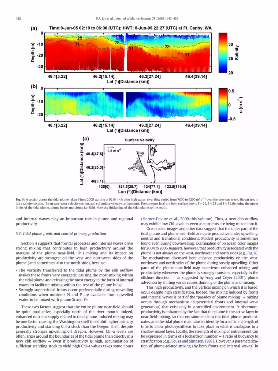
Fig. 14. A section across the tidal plume taken 9 June 2005 starting at 0219, ~4 h after high water; river flow varied from 7800 to 9200 m3 s−1 over the previous week. Shown are: in(a) a salinity section, (b) an east–west velocity section, and (c) surface velocity components. The contours in a) are from surface down, S=24, S=28 and S=31, denoting the upperlimits of the tidal plume, plume bulge and plume far-field. Note the thickening of the tidal plume to the south.


and internal waves play an important role in plume and regionalproductivity.

5.3. Tidal plume fronts and coastal primary production

Section 4 suggests that frontal processes and internal waves drivestrong mixing that contributes to high productivity around themargins of the plume near-field. This mixing and its impact onproductivity are strongest on the west and northwest sides of theplume (and sometimes also the north side), because:

• The vorticity transferred to the tidal plume by the ebb outflowmakes these fronts very energetic, causing the most mixing withinthe tidal plume and releasing themost energy in the form of internalwaves to facilitate mixing within the rest of the plume bulge.

• Strongly supercritical fronts occur preferentially during upwellingconditions when nutrients N and P are available from upwelledwater to be mixed with plume Si and Fe.

These two factors suggest that the entire plume near-field shouldbe quite productive, especially north of the river mouth. Indeed,enhanced nutrient supply related to tidal-plume-induced mixing maybe one factor causing the Washington shelf to exhibit higher primaryproductivity and standing Chl-a stock than the Oregon shelf, despitegenerally stronger upwelling off Oregon. However, Chl-a levels areoften larger around the boundaries of the tidal plume than directly in anew ebb outflow — even if productivity is high, accumulation ofsufficient standing stock to yield high Chl-a values takes some hours

(Horner-Devine et al., 2009-this volume). Thus, a new ebb outflowmay exhibit low Chl-a values even as nutrients are being mixed into it.

Ocean color images and other data suggest that the outer part of thetidal plume and plume near-field are quite productive under upwelling,neutral and transitional conditions. Modest productivity is sometimesfound even during downwelling. Examination of 56 ocean color imagesfor 2004 to 2005 suggests, however, that productivity associatedwith theplume is not always on the west, northwest and north sides (e.g., Fig. 6).The mechanisms discussed here enhance productivity on the west,northwest and north sides of the plume during steady upwelling. Otherparts of the plume near-field may experience enhanced mixing andproductivity whenever the plume is strongly transient, especially in theoffshore direction — as suggested by Fong and Geyer (2001), plumeadvection by shifting winds causes thinning of the plume and mixing.

This high productivity, and the vertical mixing on which it is based,occur despite high stratification. Indeed, the mixing induced by frontsand internal waves is part of the “paradox of plume mixing” — mixingoccurs through mechanisms (supercritical fronts and internal wavegeneration) that exist only in a stratified environment. Furthermore,productivity is enhanced by the fact that the plume is the active layer innear-field mixing, so that entrainment into the tidal plume predomi-nates, and the tidal plumemaintains its identity for a sufficient length oftime to allow photosysnthesis to take place in what is analogous to ashallowmixed layer. Locally, the strength of mixing or entrainment canbe expressed in terms of a Richardson number— a ratio of buoyancy tostratification (e.g., Souza and Simpson,1997). However, a parameteriza-tion of plume-related mixing (by both fronts and internal waves) in


terms of the bulk plume properties (e.g., river discharge, estuary mouthwidth and initial density difference) is lacking.

5.4. Salmonids and the seasonality of plume processes

There is an important connection between the plume mixingprocesses discussed here and survival of the Pacific Northwest'sendangered salmonids. Persistent upwelling typically begins in lateJune (Hickey,1989), and the seasonal timing of upwelling has changedlittle over time, at least as judged by the timing of the spring transition(Logerwell et al., 2003). Though some out-migration occurredthroughout the year, the largest number of juvenile salmonids alsocame downstream in late June and July (Bottom et al., 2005), just intime to utilize secondary productivity based on upwelled nutrients.Historically, this out-migrationwas associated with the spring freshet;now it is set by hatchery schedules.

A striking change has taken place in the Columbia River flow cycleover the last 125 years (Bottom et al., 2005), de-synchronizing it withthe onset of upwelling and salmonid behavior. The peak river flow hasshifted from late June prior to 1900 to late May. The freshet continuestomigrate to earlier dates, because of an earlier snowmelt and humanalteration of the flow cycle. Moreover, the average and freshet peakflows have decreased ~15% and N40%, respectively, mostly due tohuman factors. Thus, before 1900, a large freshet peak typicallyoccurred in late June about the same time as the onset of strongupwelling. This combination of high river flow and strong upwellingprovided high levels of N, P, Si and micronutrients to the plume areaand Oregon and Washington shelves. The frontal processes discussedhere facilitated mixing of plume and upwelled nutrients. Moreover,colder water temperatures and the shorter residence time of water inthe historical river (without dams) likely caused the system to providemore nutrients to coastal waters than at present (Small et al., 1990).Thus, even if the largest historic freshets suppressedmixing for a time,productivity could have been supported by plume nutrients (cf. Fig. 2).

High levels of primary productivity (and the secondary productionit supported) during and after the spring freshet must have providedseaward migrating juvenile salmonids with an ample food source.Also, the higher historic sediment load (at least double modern levels;Bottom et al., 2005) associated with larger historic freshets providedjuvenile salmonids with protection from predation (Pearcy, 1992).While a full understanding of the support of salmonid survival by thecoastal ecosystem remains elusive, the growing mismatch betweenthe peak river flow (now late May) and the onset of upwelling and thepeak of the juvenile salmonid migration (late June) may limit theability of the coastal ocean to support juvenile salmonids.

Acknowledgements

This research was funded by the Bonneville Power Administrationand NOAA-Fisheries (project: Ocean Survival of Salmonids), and theNSF (project RISE — River Influences on Shelf Ecosystems OCE0239072). Thanks to Ed Dever of Oregon State University for thecurrent meter data in Fig. 4. We also thank Captain Ron L. Short of theR/V Pt Sur and Marine Technicians Stewart Lamberdin, ChristinaCourcier, and Ben Jokinen for their superb support of in-situ datacollection. The SAR images were provided by Comprehensive LargeArray-data Stewardship System (CLASS) of National Oceanic andAtmospheric Administration (NOAA). Thanks to Nate Mantua andAlan Hamlet of the University of Washington for discussion of theconnection between salmonid survival and freshet timing.

References

Barnes, C.A., Duxbury, C., Morse, B.-A., 1972. Circulation and selected properties of theColumbia River plume at sea. In: Pruter, A.T., Alverson, D.L. (Eds.), The ColumbiaRiver Estuary and Adjacent Ocean Waters. University of Washington Press, Seattle,WA, pp. 41–80.

Bottom, D.L., Simenstad, C.A., Burke, J., Baptista, A.M., Jay, D.A., Jones, K.K., Casillas, E.,Schiewe, M.H. 2005. Salmon at river's end: The role of the estuary in the decline andrecovery of Columbia River salmon. U.S. Dept. of Commerce, NOAA Tech. Memo.,NMFS-NWFSC-68, 246 pp.

Chao, S.-Y., 1988. Wind-driven motion of estuarine plumes. J. Phys. Oceanogr. 18,1144–1166.

Chao, S.-Y., 1990. Tidal modulation of estuarine plumes. J. Phys. Oceanogr. 20,1115–1123.Cudaback, C.N., Jay, D.A., 1996. Buoyant plume formation at the mouth of the Columbia

River— an example of internal hydraulic control? In: Aubrey, D.G., Friedrichs, C. (Eds.),Buoyancy Effects on Coastal and Estuarine Dynamics. AGU Coastal and EstuarineStudies, vol. 53. American Geophysical Union, Washington, DC, pp. 139–154.

Cudaback, C.N., Jay, D.A., 2000. Tidal asymmetry in an estuarine pycnocline: I. Depth andthickness. J. Geophys. Res. 105, 26,237–26,252.

Fong, D.A., Geyer, W.R., 2001. Response of a river plume during and upwelling favorablewind event. J. Geophys. Res. 106, 1067–1084.

Fong, D.A., Geyer, W.R., Signell, R.P., 1997. Thewind-forced response of a buoyant coastalcurrent: observations of the western Gulf of Maine plume. J. Mar. Sys. 12, 69–81.

Garcia-Berdeal, Hickey, B.M., Kawase, M., 2002. Influence of wind stress and ambient flowon ahighdischarge river plume. J. Geophys. Res.107, 3130. doi:10.1029/ 2001JC000392.

Garvine, R.W., 1982. A steady-state model for buoyant surface plume hydrodynamics incoastal waters. Tellus 34, 293–306.

Hickey, B.M.,1989. Patterns and processes of shelf and slope circulation. In: Landry, M.R.,Hickey, B.M. (Eds.), Coastal Oceanography of Washington and Oregon. ElsevierScience, Amsterdam, pp. 41–115.

Hickey, B.M., Pietrafesa, L.J., Jay, D.A., Boicourt, W.C., 1998. The Columbia River plumestudy — subtidal variability in the velocity and salinity fields. J. Geophys. Res. 103,10339–10368.

Hickey, B.M., Geier, S.L., Kachel, N.B., MacFadyen, A., 2005. A bi-directional river plume:the Columbia in summer. Cont. Shelf Res. 25, 1631–1656.

Horner-Devine, A.R., 2009. The bulge circulation in the Columbia River plume. Cont.Shelf Res 29, 234–251.

Horner-Devine, A.R., Fong, D.A., Monismith, S.G., Maxworthy, T., 2006. Laboratoryexperiments simulating a coastal river discharge. J. Fluid Mech. 555, 203–232.

Horner-Devine, A.R., Jay, D.A., Orton, P.M., Spahn, E.Y., 2009. A conceptual model of thestrongly tidal Columbia plume. J. Mar. Sys 78, 460–475 (this volume).

Jay, D.A., Orton, P.M., Chisholm, T., 2002. Speculations on Human and Climate-ChangeAlteration of Iron Input to Upwelling Areas off Oregon and Washington, EasternPacific Ocean Conference, Timberline Lodge, OR, September 2002.

Landry, M.R., Postel, J.R., Peterson, W.K., Newman, J., 1989. Broad-scale distributionalpatterns of hydrographic variables on the Washington/Oregon shelf. In: Landry, M.,Hickey, B.M. (Eds.), Coastal Oceanography of Washington and Oregon. Elsevier,Amsterdam, pp. 1–40.

Logerwell, E.A., Mantua, N., Lawson, P.W., Francis, R.C., Agostini, V.N., 2003. Trackingenvironmental processes in the coastal zone for understanding and predictingOregon coho (Oncorhynchus kisutch) marine survival. Fish. Oceanogr. 12, 554–568.

Lohan, M.C., Bruland, K.W., 2006. Importance of Vertical Mixing for Additional Sourcesof Nitrate and Iron to Surface Waters of the Columbia River Plume: Implications forBiology. Mar. Chem. 98, 260–273.

Macdonald, D.G., Geyer,W.R., 2004. Turbulent energy production andentrainment at a highlystratified estuarine front. J. Geophys. Res. 109, C05004. doi:10.1029/2003JC002094.

Nash, J.D., Moum, J.N., 2005. River plumes as a source of large-amplitude internal wavesin the coastal ocean. Nature 43, 400–403.

O'Donnell, J., Marmorino, G.O., Trump, C.L., 1998. Convergence and downwelling at ariver plume front. J. Phys. Oceanogr. 28, 1481–1495.

O'Donnell, J., Ackleson, S.G., Levine, E.R., 2008. On the spatial scales of a river plume. J.Geophys. Res. 113, C04017. doi:10.1029/2007JC004440.

O’Reilly, J.E., Maritorena, S., Mitchell, B.G., Siegel, D.A., Carder, K.L., Garver, S.A., Kahru,M., McClain, C., 1998. Ocean color chlorophyll algorithms for SeaWiFS. J. Geophys.Res. 103, 24,937–24,953.

Orton, P.M., Jay, D.A., 2005. Observations at the tidal plume front of a high-volume riveroutflow. Geophys. Res. Lett. 32, L11605. doi:10.1029/2005GL022372.

Pan, J., Jay, D.A., 2008. Dynamic characteristics and horizontal transports of internalsolitons generated at the Columbia River plume front. Cont. Shelf Res 29, 252–262.

Pan, J., Jay, D.A., Orton, P.M., 2007. Analyses of internal solitary waves generated at theColumbia River plume front using SAR imagery. J. Geophys. Res. 112, C07014.doi:10.1029/2006JC003688.

Pearcy, W.G., 1992. Ocean Ecology of North Pacific Salmon, Washington Sea GrantProgram. University of Washington Press, Seattle, WA. 179 pp.

Small, L.F., McIntire, C.D., Macdonald, K.B., Lara-Lara, J.R., Frey, B.E., Amspoker, M.C.,Winfield, T., 1990. Primary production, plant and detrital biomass, and particletransport in the Columbia River Estuary. Prog. Oceanogr. 25, 175–210.

Souza, A.J., Simpson, J.H., 1997. Controls on stratification in the Rhine ROFI system.J. Mar. Sys. 12, 311–323.

Spahn, E.Y., Horner-Devine, A.R., Nash, J., Jay, D.A., submitted for publication. Particleprocesses in the Columbia River plume near-field, Submited to J. Geophys. Res.

Thomas, A.C., Weatherbee, R.A., 2005. Satellite-measured temporal variability of theColumbia River plume. Remote Sens. Environ. 100, 167–178.

Van Mol, B., Ruddick, K., 2005. Total Suspended Matter maps from CHRIS imagery of asmall inland water body in Oostende, Proceedings of the 3rd ESA CHRIS/ProbaWorkshop, 21–23 March, ESRIN, Frascati, Italy, (ESA SP-593, June 2005).

Yankovsky, A.E., Chapman, D.C., 1997. A simple theory for the fate of buoyant coastaldischarges. J. Phys. Oceanogr. 27, 1386–1401.

http://dx.doi.org/10.1029/ 2001JC000392

http://dx.doi.org/10.1029/2003JC002094

http://dx.doi.org/10.1029/2007JC004440

http://dx.doi.org/10.1029/2005GL022372

http://dx.doi.org/10.1029/2006JC003688

Documents

Asymmetry of Tidal Plume Fronts in an Eastern Boundary Current Regime