Ship plume modelling in EOSTAR

M. van Iersel *a

, A. Mack b, M.A.C. Degache

a, and A.M.J. van Eijk

a

a TNO, Oude Waalsdorperweg 63, 2597 AK The Hague, The Netherlands

b TNO, Stieltjesweg 1, 2628 CK Delft, The Netherlands

ABSTRACT

The EOSTAR model aims at assessing the performance of electro-optical (EO) sensors deployed in a maritime surface

scenario, by providing operational performance measures (such as detection ranges) and synthetic images. The target

library of EOSTAR includes larger surface vessels, for which the exhaust plume may constitute a significant signature

element in the thermal wavelength bands. The main steps of the methodology to include thermal signatures of exhaust

plumes in EOSTAR are discussed, and illustrative examples demonstrate the impact of the ship’s superstructure, the

plume exit conditions, and the environment on the plume behavior and signature.

Keywords: Exhaust plumes, atmospheric propagation, transmission, radiance, IR signatures, modelling

1. INTRODUCTION

The past decades have seen a proliferation of more and more technologically advanced electro-optical (EO) sensors.

These sensors are deployed in a multitude of applications, where their capability to generate images has been particularly

useful, such as in the identification of objects and the assessment of their intentions. However, when deployed in the

field, the limiting factor of these imaging systems is often not of a technological nature, but determined by the

environmental conditions. The intervening atmosphere between the object and the imaging sensor degrades the

performance. Molecules and aerosols in the atmosphere cause scattering and absorption of radiation, resulting in

transmission losses. Spatial and temporal fluctuations in the temperature and humidity of the atmosphere induce

inhomogeneities in the refractive index, which in turn are responsible for the blurring and scintillation in an image.

The presence of non-natural objects in the atmosphere may lead to further degradation of image quality. Exhaust plumes

of aircraft or ships alter the natural composition of the atmosphere by introducing a different mixture of gases at higher

temperature and density. Mixing of these hot exhaust gases with the surrounding air are the cause of turbulence effects in

the so-called plume region, which extends to some distance from the exhaust. Typical values of the refractive index

structure parameter, Cn2, for an exhaust plume (over a relatively short path) are of the order of 10

-10 m

-2/3. The presence

of an exhaust plume can thus cause severe blurring and scintillation in optical paths that intersect with the plume region,

in addition to enhanced transmission losses due to the hot and concentrated gases in the plume. This is an important

effect for e.g. directed infrared countermeasure (DIRCM) systems, which use a directed laser to counter a threat from

e.g. a missile. Several studies1-3

provide a good overview of laser beam propagation through a turbulent region of the

atmosphere, like a jet engine plume.

This paper focuses on ship exhaust plumes. While the temperatures in these ship exhaust plumes are not as high as the

plumes of jet engines and the effects in the image are thus less severe, the plume temperature is still a few hundred

degrees higher than the surrounding atmosphere resulting in a reasonable loss of transmission. Engine settings and type

of engine (diesel or gas turbine), speed and engine power have an influence on the size of the exhaust plume and on the

concentration of species (predominantly CO2, H2O, and CO) present in it. Since the plume exit velocity is lower than that

of a jet plume, the interaction with external parameters such as the wind field becomes more prominent. This does not

only apply to the larger-scale plume dispersion in the atmosphere, but also to the initial dynamics that are influenced by

the interaction of the wind field with the ship’s superstructure. An analysis of the influence of the aforementioned

parameters on the characteristics of the plume, such as spatial coverage and infrared (IR) signature of the exhaust plume

will be presented. To calculate the IR signature of the exhaust plume one needs to calculate the radiation by the gas in

the exhaust plume as well as the transmission through the plume. The gas radiation calculations are performed by a

modified version of NIRATAM.4 A computational fluid dynamics (CFD) model is used to provide information on the

* miranda.vaniersel@tno.nl

3D flow field of the exhaust plume (spatial coverage, gas concentrations, densities, and temperatures), which then can be

used as input to the gas radiation calculations.

Ultimately, the ship exhaust plume will be introduced as a scene element in the EOSTAR Pro model suite developed by

TNO The Hague in cooperation with the Royal Netherlands Navy and SPAWAR Systems Center Pacific San Diego.5-7

The EOSTAR model aims at providing an end-to-end solution for the assessment of sensor performance against a

specific threat in a specific (maritime) environment. Thus, the radiant intensities of the target8 and its background

9 are

evaluated as function of the environmental conditions.10,11

. In contrast with other ship signature prediction models such

as ShipIR12

, the CFD calculations of the ship exhaust plume will not be directly coupled to EOSTAR.

The present paper discusses the methodology to evaluate the spatial and temporal extent of the exhaust plume, as well as

the calculation of radiation of and transmission through the plume. The effect of specific plume exit conditions, and the

interaction with the ship’s superstructure and the environmental conditions are illustrated. The pathway for coupling with

EOSTAR is discussed.

2. METHODOLOGY

The methodology to evaluate the radiation of an exhaust plume and the transmission through this plume consists of

several steps, which are explained in more detail in the next subsections. The first step exploits CFD calculations to

determine the 3D flow field of the plume. This flow field serves as input to the gas radiation calculations performed by

the modified version of NIRATAM, which yields as output the IR signature of the exhaust plume. This signature will be

coupled to EOSTAR.

2.1 CFD calculations

Computational Fluid Dynamics (CFD) is used to model the 3D flow field around a ship and its plume. Included in these

calculations are the turbulent mixing effects of the hot exhaust gases with the ambient air and the interaction with the

ship geometry itself. The CFD model consists of the Reynolds Averaged Navier-Stokes (RANS) equations with a

standard k- closure for turbulence, which are solved using Ansys Fluent.13

The output parameters of the calculations are

the position coordinates (x, y, z), and for each coordinate, the pressure, density and temperature of the flow field. After

conclusion of the CFD-run, the output is reduced by selecting the local part of the numerical CFD domain containing the

exhaust plume, which is then interpolated on a mesh of 100 x 100 x 50 points. This will then serve as input for the gas

radiance calculations.

Input parameters to the CFD calculations are the wind speed and direction, the atmospheric air temperature, ship speed

and heading, engine power, the temperature of the exhaust gas, the speed of the exhaust gas at the exit plane and a

geometrical representation of the ship’s superstructure. For the studies presented in this paper, a simplified geometry of

the Royal Netherlands Navy M-frigate was used (Figure 1). The simplified geometry allows identifying the macroscopic

interactions between the undisturbed wind field, the ship’s superstructure, and the plume flow field. For the present

study, detailed and local flow fields at specific locations of the ship are not required, and a simplified geometry thus

suffices.

Figure 1: Dutch M-frigate and the simplified geometry used in the CFD calculations.

The exhaust gas composition at the exhaust exit plane is specified. In the first implementation, only three gasses (CO2,

H2O, and CO) are considered as constituents of the plume. It is assumed that no further chemical reactions take place;

hence, the mixing of the exhaust gas species with ambient air can be considered as passive. The exhaust gas is modelled

as one component (air), and it is further assumed that the thermal and mass diffusion processes behave similarly with

respect to the momentum diffusion (identical Schmidt and Prandtl numbers). In that case, the temperature distribution of

the plume serves as an indicator for the mixing process. and the concentrations of the relevant gasses (CO2, H2O, and

CO) are obtained from the temperature distribution. More specifically, the molar fractions of H2O, CO2, and CO, denoted

by CX, are derived from the temperature field T using

(

)

, (1)

with Tref the temperature of the ambient air, Tmax the temperature of the plume at the exhaust (stack), and CX,max the molar

fraction of the species at the exhaust. The factor F (equal to 1.005) is a correction factor that results from the simplified

approach of considering momentum diffusion only. The value of F was established from CFD-calculations that included

all mass and thermal diffusion processes explicitly, and allows mapping the results of the simplified approach on those of

the full calculations.

The calculations presented in this paper were conditioned by setting the temperature of the ambient air to 300 K.

Experimental data yielded the initial (maximum) temperature of the exhaust gases (633 K, corresponding to 100% power

setting) and the maximum molar fractions Cmax(CO2) = 0.037, Cmax(CO) = 0.00015, and Cmax(H2O) = 0.037. Here, the

maximum molar fractions are taken as constant since no load dependent values were available.

2.2 Plume radiation calculations

The radiant intensity of the exhaust plume is calculated using a modified version of the NATO Infrared Air Target

Model (NIRATAM).4 The major modification consists of replacing the (2D) rotation-symmetric exhaust plume provided

by NIRATAM’s sub-model N-plume by the (asymmetric (3D)) ship exhaust plume provided by the CFD code discussed

in the previous section. Furthermore, the aircraft model in NIRATAM was replaced by a rudimentary ship model. The

gas radiation calculations constitute, also in this modified version, the core of NIRATAM.

The radiant intensity of the exhaust plume results from three effects: (1) spectral emission lines determined by the

composition and temperature of the gases; (2) broadband (Planck) radiation determined by the temperature of the gases;

(3) (spectral) absorption of the radiance by the plume itself. The spectral lines denote transitions between the vibrational-

rotational energy levels of a molecule. Each vibration in the molecule gives rise to a band of spectral lines with energies

corresponding to the common vibrational transition energy offset by the various rotational sub-transitions. The

fundamental lines are broadened by the Doppler effect and by collisions between the molecules. Ideally, the radiant

intensity is calculated by a summation of all individual lines, but this process is time-consuming and often the transition

cross-sections are not precisely known. Therefore, NIRATAM uses band-line models in which the spectrum is divided in

several intervals / bands. A single-line group (SLG) model or a multi-line group (MLG) model can be used to calculate

the spectrum. In a SLG model all lines within an interval are treated as if they represent a single line. In a MLG model

the lines in an interval are divided into groups such that all lines in a group have similar strengths. In both models the

Curtis-Godson approximation is used to replace the inhomogeneous concentration of the species in an interval with a

homogeneous concentration.

For a specified sensor-plume viewing geometry, NIRATAM divides the exhaust plume in segments and passes a number

of rays through the plume along the line of sight of the sensor. For each segment the contribution to the radiation in the

wavelength band of the sensor is added to a running sum of the total radiation along the line of sight. The radiation

transfer equations and spectral information are taken from literature.14

The Planck radiation and the spectral line

contributions of the molecules H2O, CO2, and CO in the exhaust plume are evaluated. Also included in the calculations

are the molecules H2, N2, and O2. While these do not yield vibrational-rotational spectral emission line because of the

absence of an electric dipole moment, they contribute to the line broadening of the spectral lines of the other molecules.

Furthermore, the transmission through the exhaust plume is calculated.

The 3D flow fields calculated with the CFD code are input for the calculations with the modified version of NIRATAM.

A list of additional input parameters can be found elsewhere,15

which includes the background temperature and

emissivity, wavelength or wavenumber interval, a characterization of the atmosphere, and the sensor – plume viewing

geometry. As an output NIRATAM can produce image files containing the radiant intensity, radiance, or apparent

temperature as well as a spectral radiance file containing the intrinsic or apparent radiance for the wavelength or

wavenumber interval. The image file is only spatially resolved and provides a 2D radiance image of the plume viewed by

the sensor. The spectral radiance file contains a spectral table of plume radiance and plume transmission. This table is

spatially not resolved and thus represents the “overall” radiance and transmission as viewed by the sensor.

NIRATAM offers the added feature of calculating the atmospheric transmission outside the plume. This can be done by

the internal LOWTRAN module, or by an external coupling to MODTRAN. If activated, this calculation thus yields the

total signal received at the sensor as the sum of two parts; the radiation of the plume transmitted through the atmosphere

over a path between plume and sensor and the transmission of the background radiation through the atmosphere over a

path between background and plume, then through the exhaust plume, and finally the transmission through the

atmosphere over a path between the plume and the sensor.

2.3 EOSTAR

As already mentioned, the plume module will be coupled to the Electro-Optical Signal Transmission And Ranging

(EOSTAR) model. EOSTAR evaluates the performance of an electro-optical sensor against targets in a scene under

varying meteorological conditions. One of the central elements in EOSTAR is the Snell’s Law Ray Tracing Scheme

(SLARTS),16

which provides the ‘sensor ray trajectories’ that are the basis for evaluating the effects of atmospheric

refraction and path-integrated effects (e.g., transmission, radiance, blur, and scintillation) on the image. The ray

trajectories represent the observation paths of the individual sensor pixels and the trajectories can thus be considered as

the axes of the instantaneous field of view (IFOV) of the single detector elements of the sensor. Each trajectory is

launched from the center of this pixel, crosses the middle of the optics and starts its propagation path in the atmosphere

at the position and at the azimuth and elevation angles corresponding to the particular detector element. The fan of ray

trajectories covers the field-of-view of the sensor.

In order to calculate the ray trajectories through the atmosphere, EOSTAR first evaluates the fields of pressure,

temperature and humidity, using (a combination of) Monin-Obukhov similarity theory, radiosonde observations and

numerical weather prediction data,10,11

and from these, the field of refractive index. The fields of pressure, temperature

and humidity, as well as various other parameters that characterize the atmosphere, are also used to drive MODTRAN

for the evaluation of molecular transmission, and ANAM for the evaluation of aerosol extinction in a maritime

environment. Finally, the field of the refractive index structure-function parameter Cn2 can be evaluated, which quantifies

turbulence effects (scintillation, blur) on the image.

The trajectories are constructed as a series of small steps (typically 50 m). At each step, the local ray direction and local

refractive index gradient are used to evaluate the change in ray direction due to refraction in a spherically stratified

atmosphere. At the same time, the transmission losses due to molecular and aerosol extinction are evaluated over the

step, and the overall transmission from the sensor to the current ray position. Neighboring rays are used to evaluate the

local geometric distortion, i.e., the phenomenon that refractive effects cause the pixel IFOV to deviate from R2. The

geometric gain factor and the transmission losses together specify the propagation factor, i.e., the transfer function for

radiant intensity between the sensor and the ray position. When an object (e.g., a ship) with a specific radiant intensity is

positioned in the scene, the ray tracer thus provides the distribution of detector IFOVs over the target and all the

information required to evaluate the radiant intensity of the target on the sensor.

The coupling of the exhaust plume to EOSTAR will initially be done by file transfer. Intermediate results of the modified

version of NIRATAM are written to file. These results contain the spatially and spectrally resolved radiation of the

exhaust plume (without propagation through a NIRATAM atmosphere), calculated for the same sensor characteristics

and sensor – target geometry as EOSTAR will use. EOSTAR reads in the file and positions the plume on top of the

exhaust of the ship, thereby completing the target signature. EOSTAR then calculates the radiant intensity of the

complete target received at the sensor.

EOSTAR provides a synthetic image of the scene as perceived by the sensor as output. Another output of EOSTAR

consists of range-height and range-azimuth coverage diagrams of quantities of interest (e.g., detection range). When

building coverage diagrams, EOSTAR takes target constraints into account, e.g., the constraint that a ship must be at the

surface, whereas an aircraft can be at any altitude.

3. RESULTS

The size, temperature distribution and shape of an exhaust plume are influenced by atmospheric parameters like the (air)

temperature, wind speed and direction, as well as by engine settings like engine power, speed, and type of engine. These

parameters also have an influence on the radiant intensity of the exhaust plume and the transmission through the plume.

The sections below addresses the influence of several of these parameters on the radiant intensity and transmission

through the exhaust plume.

All calculations have been made with the model of the Royal Netherlands Navy M-frigate (see Figure 1). The speed

vector, v, is a combination of the ship’s speed vector and the wind speed vector. The combined speed vector is denoted

by a length v and a direction θ. The ship is assumed to sail in a heading of 0°. A wind direction of 0° is defined as head

on to the bow of the ship. A homogeneous background with a temperature of 300K is used in the simulations. The sensor

is positioned behind and to the left of the ship, with a range R = 2km.

3.1 Output of modified version of NIRATAM for the case v = 15 m/s, θ = 0°, engine power = 100%

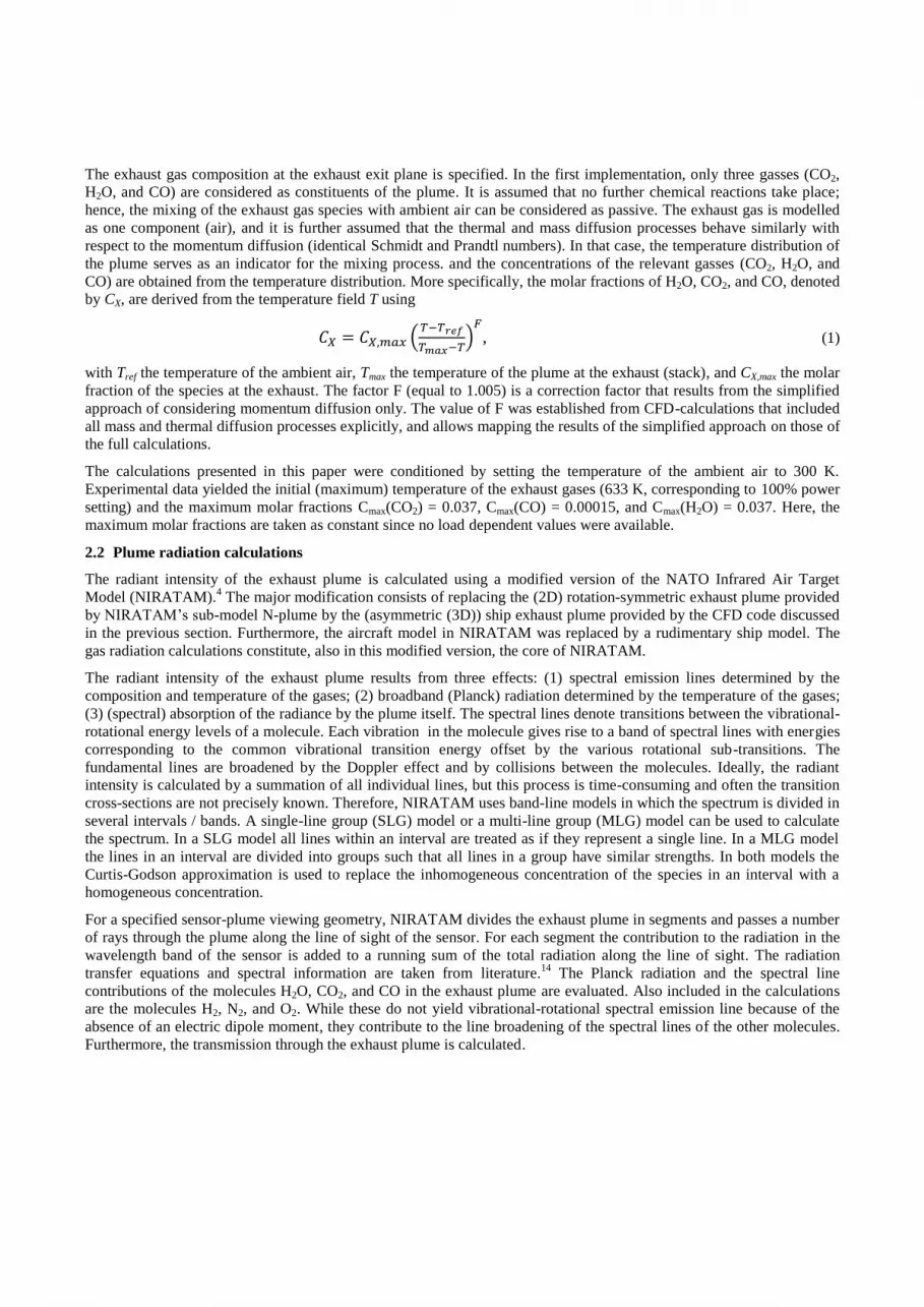
In this case, which will serve as a reference later on, the combined speed is v = 15 m/s and the direction θ = 0° (head on).

The engine power is set to 100% and other conditions are as mentioned in section 2.1. The modified version of

NIRATAM provides a radiant intensity image, as well as the apparent or intrinsic radiance, and the contrast intensity of

the object (plume) against the background. An example of a radiance map is shown in Figure 2a. Note that these images

are spatially resolved, but not spectrally. The example shows the radiance integrated over the band of 3.0 – 5.0 μm (3333

– 2000 cm-1

). Figure 2b presents the contrast irradiance spectrum for the wavelength band of 2.0 – 14.0 μm (5000 – 715

cm-1

), i.e., the radiant contrast between the plume and the background. Note that this output is not spatially resolved, and

thus includes the overall plume radiance and transmission. The spectrum in Figure 2b exhibits the major emission peaks

of CO2, CO, and H2O, which lead to a maximum contrast at those wavelengths. At other wavelengths, the contrast

intensity is zero signaling that the plume does not produce radiation at these wavelengths.

(a) (b)

Figure 1: (a) Radiance map of the exhaust plume for 3.0 - 5.0 μm and (b) the contrast irradiance spectrum of the

plume for 2.0 – 14.0 μm.

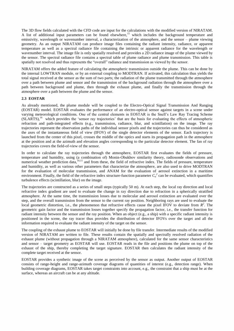
The results in Figure 2 were obtained with the additional atmosphere module of NIRATAM turned off; the results thus

represent the inherent properties of the plume. Alternatively, Figure 3 shows results with the additional atmosphere

module (external MODTRAN v4.3.1) turned on. The Figure thus displays the contrasts as perceived by the sensor

positioned at 2 km from the ship. For comparison, results obtained with the older and obsolete LOWTRAN internal

module as provided by the standard NIRATAM code are also shown. For simplicity, the mid-latitude summer scenario

with the marine aerosol model (visibility of 23 km) was used in both cases. Figure 3a shows the contrast irradiance

spectrum for 2.0 – 14.0 μm (5000 – 715 cm-1

), whereas Figure 3b presents a zoom along the vertical (contrast

irradiance) axis. Black curves denote the absence of an atmosphere (equivalent to Figure 2b), the blue and red curves

denote calculations with MODTRAN and LOWTRAN, respectively. The blue and red curves clearly demonstrate the

higher spectral resolution of the (recommended) MODTRAN code. The higher spectral resolution is required for

EOSTAR, which generally runs at a resolutions below 20 cm-1

.

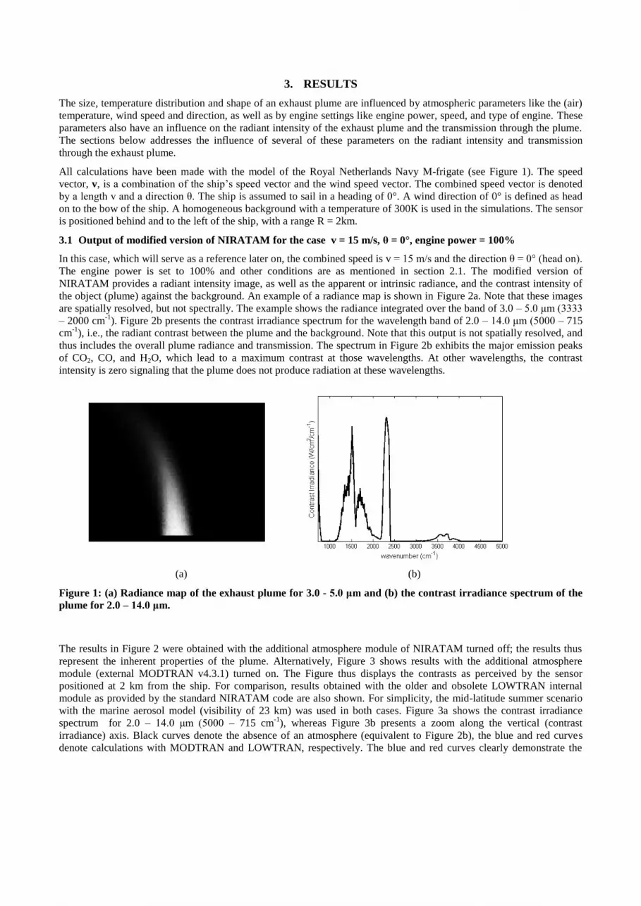
Figure 3 shows that the major emission peaks of the plume are efficiently absorbed by the atmosphere, resulting in zero

contrast over large wavelength bands. This is not surprising, since the plume constituents CO2, CO and H2O are also

abundant in the ambient atmosphere. However, the higher temperature of the exhaust gases causes line broadening,

which causes the absorption and the emission not to cancel out completely at the extreme edges of the peaks, e.g., for the

peak at 4.1 – 4.5 μm (2222 – 2439 cm-1

). The non-zero contrast peaks at either end of the peak are known as the blue and

red spikes, and are particular relevant for sensors operating in the midwave band (3 – 5 μm). As an illustration, Figure 4

shows the contrast irradiance spectrum of the peak for nominal midwave and longwave (8 – 12 μm) infrared sensors. The

figure suggests that both types of sensors may be able to detect the presence of the plume; note, however, that the

vertical scales of figures 4a and 4b are not identical.

(a) (b)

Figure 2: (a) Contrast irradiance spectrum of the exhaust plume without atmosphere (black line) and with

LOWTRAN (red line) or MODTRAN (blue line) atmospheres. (b) Zoom along the vertical axis.

(a) (b)

Figure 3: Contrast irradiance spectrum of the exhaust plume measured in midwave (a) and longwave (b) bands.

3.2 Effect of θ (angle of attack of combined speed vector)

As mentioned before, the combined speed vector results from the vector addition of the ship’s speed vector and the wind

speed vector. The direction (or angle of attack) θ = 0° corresponds to a combined speed vector onto the bow of the ship.

The direction of the combined speed vector has a significant influence on the shape and size of the exhaust plume, as

demonstrated by Figure 5. The Figure shows three radiance maps for three angles of attack (a-c), as well as a plot of the

maximum plume contrast as function of angle of attack (d). The calculations were made for a combined speed v = 15

m/s, engine power of 100%, the midwave infrared band (3.0 – 5.0 μm), the MODTRAN atmosphere (see previous

section) and show the radiance as perceived by the sensor at 2 km distance, located to the left of the ship. Figure 5d also

shows results for LOWTRAN and the absence of an atmosphere.

The shape of the plume is clearly different for the different directions (different angles of attack of the wind). The plume

for θ = 30° stays much lower compared to the plumes for 0° and 90°. In accordance with this, Figure 5d shows that the

minimum radiant intensity occurs at θ = 20° and that the maximum occurs at θ = 0°. The explanations for the observed

behavior of the plume can be related to the geometry of the M-frigate and the streamlines on the ship’s surface (not

shown here).

(a) (b)

(c) (d)

Figure 4: Radiance maps of the exhaust plume at the midwave IR-sensor for (a) θ = 0°, (b) 30°, and (c) 90°. (d)

Maximum contrast irradiance vs. angle of attack in the absence of atmosphere (black line), or with LOWTRAN

(red line) and MODTRAN (blue line) atmospheres.

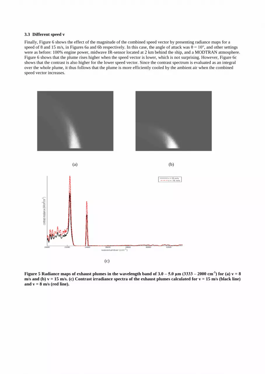
3.3 Different speed v

Finally, Figure 6 shows the effect of the magnitude of the combined speed vector by presenting radiance maps for a

speed of 8 and 15 m/s, in Figures 6a and 6b respectively. In this case, the angle of attack was θ = 10°, and other settings

were as before: 100% engine power, midwave IR-sensor located at 2 km behind the ship, and a MODTRAN atmosphere.

Figure 6 shows that the plume rises higher when the speed vector is lower, which is not surprising. However, Figure 6c

shows that the contrast is also higher for the lower speed vector. Since the contrast spectrum is evaluated as an integral

over the whole plume, it thus follows that the plume is more efficiently cooled by the ambient air when the combined

speed vector increases.

(a) (b)

(c)

Figure 5 Radiance maps of exhaust plumes in the wavelength band of 3.0 – 5.0 μm (3333 – 2000 cm-1

) for (a) v = 8

m/s and (b) v = 15 m/s. (c) Contrast irradiance spectra of the exhaust plumes calculated for v = 15 m/s (black line)

and v = 8 m/s (red line).

4. CLOSING REMARKS

The previous sections present the methodology for including (ship) exhaust plumes in the EOSTAR model suite, which

aims at assessing the performance of electro-optical sensors in a maritime environment. Although the methodology

allows capturing several of the characteristic plume elements like dispersion, radiance and transmission as function of

internal (engine settings) and external (atmospheric) parameters, only a rough framework is in place at this stage,

especially where it concerns the coupling with EOSTAR. Obviously, further development may include the scientific

improvement of individual modules, e.g., by incorporating additional species in the plume such as black carbon. In our

opinion, however, it is more important to first optimize the coupling with EOSTAR that will allow us to study the effect

of the plume on sensor performance measures such as detection range.

EOSTAR is intended for use in an operational context, which leads to the requirement that the sensor performance

measures can be calculated within relatively short time. This implies that the CFD-calculations must be performed as an

offline process before the actual operational deployment of EOSTAR. The results of the CFD-calculations should thus be

stored in a database of pre-calculated plumes. The example of the ship-plume interaction given in section 3.2 suggests

that each individual target in the EOSTAR database requires its own set of exhaust plumes. Within a specific set (or in

other words, for a specific platform or target), certain parameters are constant (e.g., the geometry of the exhaust stack,

and the position of the stack on the platform). However, there remains a relatively large number of free parameters

(engine power, wind speed, wind direction, etc), which thus implies that the database of pre-calculated plumes has to be

quite large. The possibility of establishing approximate relations between the free parameters and, e.g., plume height or

plume radiance should thus be investigated to keep the size of the database manageable.

The NIRATAM calculations are also relatively time-consuming. Possibly, an optimization of the code may speed up this

process, but this is currently not under investigation. However, even though NIRATAM is relatively time-consuming

there are advantages in coupling NIRATAM more stringently with EOSTAR. The two codes share a number of input

parameters, related to the sensor specifications (wavelength band, # pixels, sensor response curve, ..) and the sensor –

target (plume) viewing geometry. A common interface would ensure that both codes use the same parameters and reduce

the possibility of errors.

The EOSTAR model suite requires a spatial, temporal and spectrally resolved representation of the plume, which is then

entered in the synthetic scene as an additional signature element. The propagation of the radiation from the plume to the

sensor, and for that matter, the propagation of background radiance through the plume and onto the sensor, must be

handled by EOSTAR. The additional MODTRAN module provided by NIRATAM (cf Figures 3, 5 and 6) cannot be

used, because this would lead to a discrepancy between EOSTAR’s ray-tracer and MODTRAN’s internal ray-tracer.

This then suggests that the EOSTAR – NIRATAM interface must consist of a transfer of fundamental plume data only.

ACKNOWLEDGEMENTS

Our colleague Ric Schleijpen is acknowledged for valuable contributions to the work presented here. The work in this

paper was performed as part of the TNO research program V1303 – Above Water Signatures, sponsored by the Ministry

of Defence of the Netherlands.

REFERENCES

[1] Sjöqvist, L., “Laser beam propagation in jet engine plume environments – a review,” Proc. SPIE 7115 (2008).

[2] Andrews, L.C. and Phillips, R.L., “Laser Beam Propagation Through Random Media,” SPIE Press (2005).

[3] Ric H. Schleijpen, “Laser pointing in the vicinity of jet engine plumes,” SPIE Vol. 7483, paper13,

Technologies for Optical Countermeasures VI (2009).

[4] Noah, M., Kristl, J., Schroeder, J., “NIRATAM – NATO Infrared Air Target Model,” Proc. SPIE 1479, 275 –

282 (1991).

[5] Kunz, G.J. , Moerman, M.M., van Eijk, A.M.J., Doss-Hammel, S.M., and Tsintikidis, D., “EOSTAR : An

electro-optical sensor performance model for predicting atmospheric refraction, turbulence and transmission in

the marine surface layer,” Proc. SPIE 5237, 81-92 (2003).

[6] Van Eijk, A.M.J., Degache, M.A.C., Tsintikidis, D., and Hammel, S., “EOSTAR Pro: a flexible extensive

library to assess EO sensor performance,” Proc. SPIE 7828 (2010).

[7] Van Eijk, A.M.J., Degache, M.A.C, and de Lange, D.J.J., “The EOSTAR model suite,” in International

Symposium on Optronics in Defense and Security, OPTRO 2010, 3-5 February, Paris, France. (2010).

[8] Neele, F.P., “Infrared ship signature prediction, model validation and sky radiance,” Proc. SPIE 5811, 180-187

(2005).

[9] Schwering, P.B.W., “IRST evaluation methodologies: Maritime infrared background simulator,” Proc. SPIE

6206 (2006).

[10] Kunz, G.J., “A bulk model to predict optical turbulence in the marine surface layer,” TNO-FEL Report Nr.

FEL-96-A053, TNO Physics and Electronics Laboratory, The Hague, The Netherlands (1996).

[11] Penelon, T., Calmet, I., and Mironov, D.V., “Mircometeorological simulations over complex terrain with

SUBMESO: a model study using a novel preprocessor,” Int. J. Env. Poll. 16, 583-602 (2001).

[12] Vaitekunas, D.A., Sideroff, Ch., and Moussa, Ch., “Improved signature prediction through coupling of ShipIR

and CFD,” Proc. SPIE 8014 (2011).

[13] ANSYS Inc., “Fluent 13 Documentation,” 2010.

[14] Ludwig, C.B., Malkmus, W., Raerdon, Y.E., and Thomson, J.A.L., “Handbook of Infrared Radiation from

Combustion Gases,” National Aeronautics and Space Administration, NASA-SP 3080 (1973).

[15] Fair, M.L., “NIRATAM Software User Guide,” TR/DERA/WSS/WX3/TR980154/1.0 (1998).

[16] Kunz, G.J., Moerman, M.M., and van Eijk, A.M.J., “ARTEAM : Advanced Ray Tracing with Earth

Atmospheric Models,” Proc. SPIE 4718, 397-404 (2002).