APPLICATION OF RANDOM FINITE ELEMENT METHOD TO BEARING CAPACITY DESIGN OF STRIP FOOTING

Vessia et al.: Application of Random Finite Element Method to Bearing Capacity Design of Strip Footing 103

Manuscript received September 1, 2009; revised December 16,2009; accepted December 21, 2009.

1 Contract researcher (corresponding author), Department of Civiland Environmental Engineering, Technical University of Bari, ViaOrabona, 4, Italy (e-mail: [email protected]).

2 Full professor, Department of Civil and Environmental Engineer-ing, Technical University of Bari, Via Orabona 4, Italy (e-mail:[email protected]).

3 Ph.D. student, Wroclaw University of Technology, WybrzeżeWyspiańskiego 27, Poland (e-mail: [email protected]).

4 Associate Professor, Wroclaw University of Technology, WybrzeżeWyspiańskiego 27, Poland (e-mail: [email protected]).

APPLICATION OF RANDOM FINITE ELEMENT METHOD TO BEARING CAPACITY DESIGN OF STRIP FOOTING

Giovanna Vessia1, Claudio Cherubini2, Joanna Pieczyńska3, and Wojciech Puła4

ABSTRACT

According to the reliability-based design approach suggested by Eurocode 7, the random finite element method has been em-ployed for calculating the reliability index for the bearing capacity design of strip foundation. Such study has been carried out on a well-defined soil from a stochastic point of view, that is the grey-blue clay from Taranto area. The RFEM formulation used has been implemented by Griffiths and Fenton but here the authors have focused on a description of the anisotropic random field for c and φ design variables. Results clearly show that the introduction of anisotropy in random fields makes RFEM predictions effec-tive for design purpose because it is less conservative and more realistic than the isotropy assumption.

Key words: RFEM, bearing capacity, strip foundation, anisotropic random field.

1. INTRODUCTION The shallow footing geotechnical design is mainly based on

the evaluation of the bearing capacity. Random character of physical and mechanical soil properties heavily influences the randomness of the bearing capacity estimation which is not usu-ally taken into account into practice.

New building codes as Eurocodes and Italian TU 2008 have absorbed the contribution of about 30 year research in random field and nowadays reliability-based design is one of the sug-gested design approaches. Nonetheless whenever 2D numerical simulations are employed for the estimation of the shallow foot-ing bearing capacity, the random finite element method (RFEM) can be used. Such a numerical methodology was introduced by Griffiths and Fenton (Griffiths and Fenton 1993; Fenton and Griffiths 1993) and employed in many applications (Griffiths and Fenton 2001; Fenton and Griffiths 2003; Griffiths et al. 2002; Griffiths and Fenton 2004; Fenton and Griffiths 2005; Griffiths et al. 2006). By now over 50 papers applying this methodology in geotechnics have been reported. RFEM connects random field theory (Vanmarcke 1984) and deterministic formulation of the finite element method by taking into account mean value, stan-dard deviation, correlation length of strength and load design parameters. Thus, implementing Terzaghi’s formula (Terzaghi 1943) into RFEM the bearing capacity can be calculated as fol-lows:

1 2f c qq c N q N BNγ= + + γ (1)

where qf is the ultimate bearing stress, c is the cohesion, q is the overburden load due to foundation embedment, γ is the soil unit weight, B is the footing width, and Nc, Nq and Nγ are the bearing capacity factors. To simplify the analysis and focus on the ran-dom character of soil parameters Eq. (1) is accordingly simplified (neglecting the contributions of both the footing embedment and the soil weight) for the case of drained conditions:

f cq c N= (2)

where the Nc expression is given below (Bowles 1996):

tan 2tan 14 2

tanc

eN

π φ π φ⎛ ⎞+ −⎜ ⎟⎝ ⎠=

φ (3)

In this paper the authors focused their attention on analyzing the influence of some relevant aspects of the random characterization of soil by means of the numerical algorithm created by Fenton and Griffiths (2003), that is: • the rule of anisotropy in random field approach to soil pa-

rameters, implemented by analyzing different values of corre-lation length along vertical and horizontal direction;

• verification of the worst case, which means that in every single situation it is possible to assign the characteristic value of cor-relation length corresponding to the most conservative evalua-tion of the bearing capacity;

• to investigate random variability of soil properties based on statistical data resulting from real soil testing. The soil under investigation is the grey-blue clay from South East of Italy.

2. THE RANDOM FIELD FORMULATION FOR SOIL

The random soil model proposed by Fenton and Griffiths (2003) describes strength soil parameters by means of isotropic two-dimensional random field by local averaging approach (Vanmarcke 1984).

Two random field variables are taken into account in this paper, that is c and φ.

Journal of GeoEngineering, Vol. 4, No. 3, pp. 103-112, December 2009

104 Journal of GeoEngineering, Vol. 4, No. 3, December 2009

The cohesion random field is assumed to be lognormal dis-tributed with mean μc, standard deviation σc and different spatial correlation lengths θcy and θcx in vertical and horizontal direction, respectively.

Theoretical aspects of the anisotropic random field assump-tion have been analyzed in earlier papers (Pula and Shahrour 2003; Pula 2004).

Lognormal random field is derived from a normally distrib-uted random field Gln c(x), having zero mean, unit variance and spatial correlation length θln c transformed as follows:

{ }ln ln ln( ) exp ( )c c cc G= μ + σx x (4)

where x is the spatial position at which c is calculated and μln c and σln c parameters are obtained as mean and standard deviation values of cohesion function:

22ln 2ln 1 c

cc

⎛ ⎞σσ = +⎜ ⎟

μ⎝ ⎠ (5)

2ln ln

1ln2c c cμ = μ − σ (6)

Such a transformation is very useful because there are many ef-fective methods for generating normal field and then using Monte Carlo simulation. Realizations of cohesion field have been calculated after having generated the realization of normal field using the transformation in Eq. (4). Correlation structure of cohe-sion lognormal field Gln c(x) is expressed by determining the cor-relation function, whose parameters are correlation lengths along the two directions θ(ln c)y and θ(ln c)x.

In this paper the following correlation function has been as-sumed:

2 2

2 1ln

(ln ) (ln )

2( ) 2( )expcc x c y

⎛ ⎞⎛ ⎞ ⎛ ⎞τ τ⎜ ⎟ρ = − +⎜ ⎟ ⎜ ⎟⎜ ⎟ ⎜ ⎟⎜ ⎟θ θ⎜ ⎟⎝ ⎠ ⎝ ⎠⎝ ⎠

(7)

where τ1 = y2 − y1 and τ2 = x2 − x1 are the two components of the absolute distance between the two points in 2D space where the

correlation function is calculated by taking into account the ani-sotropic character of the random field (θ(ln c)y and θ(ln c)). It is worth mentioning that such a correlation function works in a normal random field ln c. θ(ln c)y and θ(ln c)x values are derived from θcy and θcx values.

Correlation lengths θcy and θcx can be drawn from in situ tests. One method for converting soil testing results into correla-tion length is the moment method (Baecher and Christian 2003). Such methodology has been used in this paper.

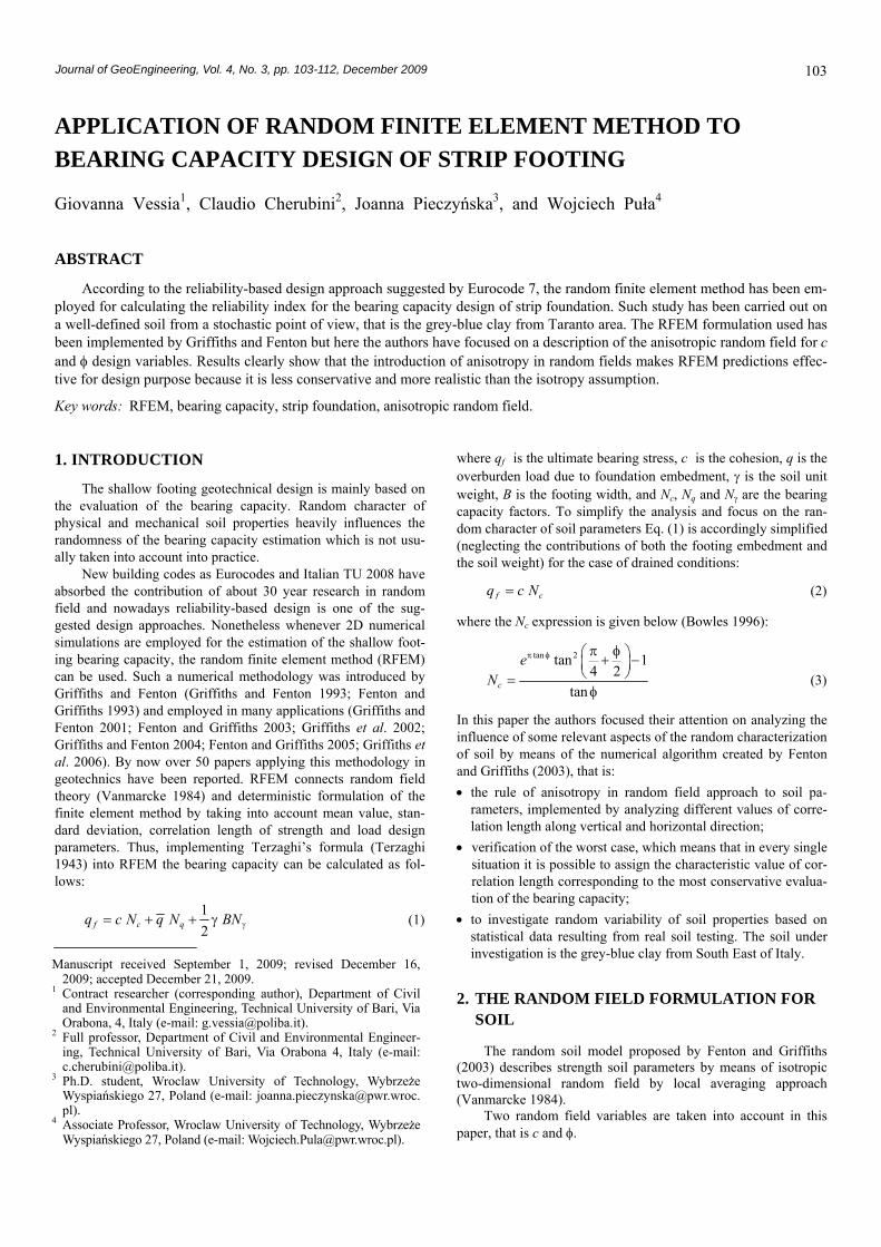
The second random field considered in this paper is the fric-tion angle. Since friction angle values change within a bounded interval, neither normal nor lognormal distributions are appropri-ate models for random variable. Fenton and Griffiths (2003) rep-resented bounded distributed fields as a bounded distribution which resembles a beta distribution but arises as a simple trans-formation of a Gφ(x), according to:

min max min( )1( ) ( ) 1 tanh

2 2sG x

x φ⎧ ⎫⎛ ⎞⎪ ⎪φ = φ + φ − φ +⎨ ⎬⎜ ⎟π⎪ ⎪⎝ ⎠⎩ ⎭ (8)

where φmin and φmax are the minimum and maximum values of friction angle, respectively, and s is the scale factor depending on standard deviation.

Shapes shown in Fig. 1 represent probability distribution functions of φ variable. In the graph, φ functions are reported for three different scale factor values s. For s values greater than 5 frequency distribution leads to a U-shaped function which is unrealistic in current situations. The mean distribution is in the middle of the interval [φmin, φmax]. Relationship between the stan-dard deviation and the scale parameter s has no analytic form. It can be obtained by numerical integration or by Taylor’s expan-sion. The first order approximation leads to:

( )max min0 0

1 2( )2 exp(2 ) exp( 2 ) 2

sφσ ≈ φ − φ

π φ + − φ + (9)

where φ0 is the mean value of the friction angle. Correlation function and correlation length values have been estimated as in the case of cohesion.

3. THE CASE STUDY OF ITALIAN BLUE-GREY CLAY

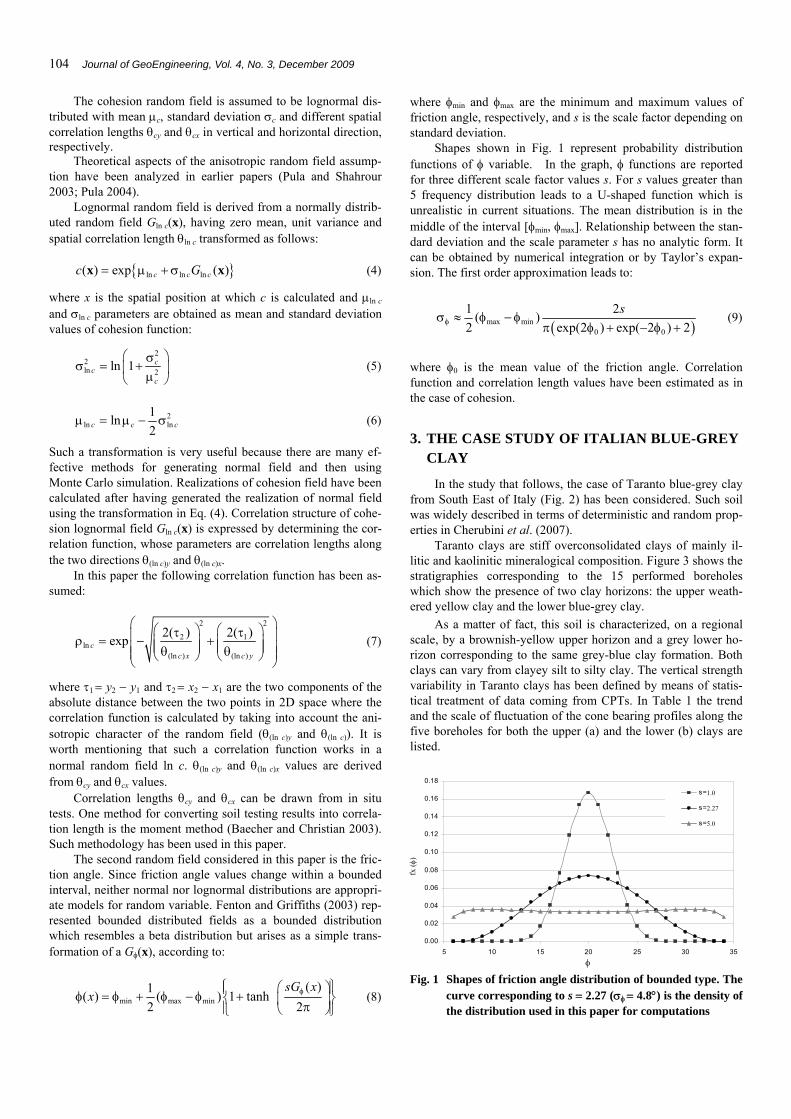
In the study that follows, the case of Taranto blue-grey clay from South East of Italy (Fig. 2) has been considered. Such soil was widely described in terms of deterministic and random prop-erties in Cherubini et al. (2007).

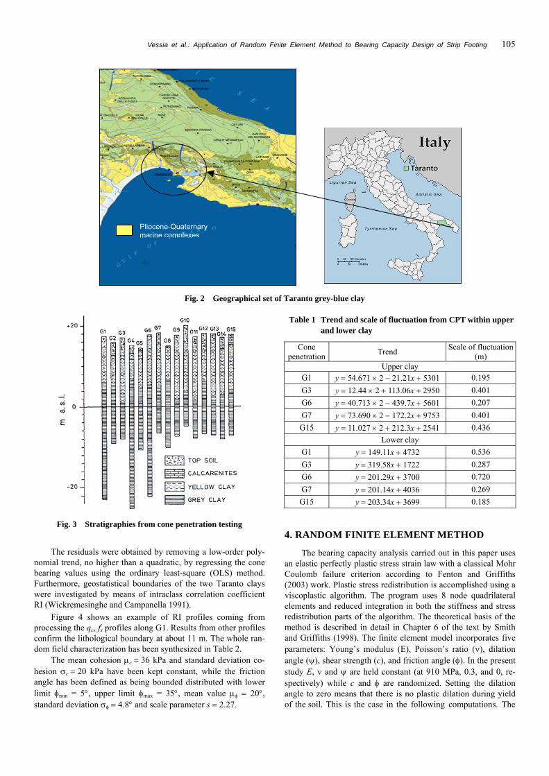
Taranto clays are stiff overconsolidated clays of mainly il-litic and kaolinitic mineralogical composition. Figure 3 shows the stratigraphies corresponding to the 15 performed boreholes which show the presence of two clay horizons: the upper weath-ered yellow clay and the lower blue-grey clay.

As a matter of fact, this soil is characterized, on a regional scale, by a brownish-yellow upper horizon and a grey lower ho-rizon corresponding to the same grey-blue clay formation. Both clays can vary from clayey silt to silty clay. The vertical strength variability in Taranto clays has been defined by means of statis-tical treatment of data coming from CPTs. In Table 1 the trend and the scale of fluctuation of the cone bearing profiles along the five boreholes for both the upper (a) and the lower (b) clays are listed.

0.00

0.02

0.04

0.06

0.08

0.10

0.12

0.14

0.16

0.18

5 10 15 20 25 30 35

fx(Φ

)

s=1,0

s=2,27

s=5,0

Fig. 1 Shapes of friction angle distribution of bounded type. The curve corresponding to s = 2.27 (σφ = 4.8°) is the density of the distribution used in this paper for computations

φ

fx (φ

)

1.0 2.27 5.0


Fig. 2 Geographical set of Taranto grey-blue clay

Fig. 3 Stratigraphies from cone penetration testing

The residuals were obtained by removing a low-order poly-nomial trend, no higher than a quadratic, by regressing the cone bearing values using the ordinary least-square (OLS) method. Furthermore, geostatistical boundaries of the two Taranto clays were investigated by means of intraclass correlation coefficient RI (Wickremesinghe and Campanella 1991).

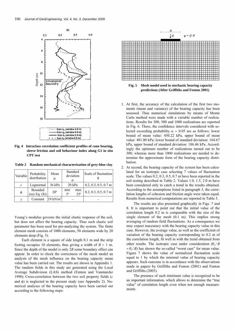
Figure 4 shows an example of RI profiles coming from processing the qc, fs profiles along G1. Results from other profiles confirm the lithological boundary at about 11 m. The whole ran-dom field characterization has been synthesized in Table 2.

The mean cohesion μc = 36 kPa and standard deviation co-hesion σc = 20 kPa have been kept constant, while the friction angle has been defined as being bounded distributed with lower limit φmin = 5°, upper limit φmax = 35°, mean value μφ = 20°, standard deviation σφ = 4.8° and scale parameter s = 2.27.

Table 1 Trend and scale of fluctuation from CPT within upper and lower clay

Cone penetration Trend Scale of fluctuation

(m) Upper clay

G1 y = 54.671 × 2 − 21.21x + 5301 0.195 G3 y = 12.44 × 2 + 113.06x + 2950 0.401 G6 y = 40.713 × 2 − 439.7x + 5601 0.207 G7 y = 73.690 × 2 − 172.2x + 9753 0.401

G15 y = 11.027 × 2 + 212.3x + 2541 0.436 Lower clay

G1 y = 149.11x + 4732 0.536 G3 y = 319.58x + 1722 0.287 G6 y = 201.29x + 3700 0.720 G7 y = 201.14x + 4036 0.269

G15 y = 203.34x + 3699 0.185

4. RANDOM FINITE ELEMENT METHOD

The bearing capacity analysis carried out in this paper uses an elastic perfectly plastic stress strain law with a classical Mohr Coulomb failure criterion according to Fenton and Griffiths (2003) work. Plastic stress redistribution is accomplished using a viscoplastic algorithm. The program uses 8 node quadrilateral elements and reduced integration in both the stiffness and stress redistribution parts of the algorithm. The theoretical basis of the method is described in detail in Chapter 6 of the text by Smith and Griffiths (1998). The finite element model incorporates five parameters: Young’s modulus (E), Poisson’s ratio (ν), dilation angle (ψ), shear strength (c), and friction angle (φ). In the present study E, ν and ψ are held constant (at 910 MPa, 0.3, and 0, re-spectively) while c and φ are randomized. Setting the dilation angle to zero means that there is no plastic dilation during yield of the soil. This is the case in the following computations. The

Pliocene-Quaternary marine complexes


Fig. 4 Intraclass correlation coefficient profiles of cone bearing,

sleeve friction and soil behaviour index along G1 in situ CPT test

Table 2 Random mechanical characterization of grey-blue clay

Variable Probability distribution

Mean μ

Standard deviation

σ

Scale of fluctuationθ

c Lognormal 36 kPa 20 kPa 0.2, 0.3, 0.5, 0.7 m

φ Bounded (see Eq. (8)) 20° min max

5° 35° 0.2, 0.3, 0.5, 0.7 m

γ Constant 19 kN/m3 − −

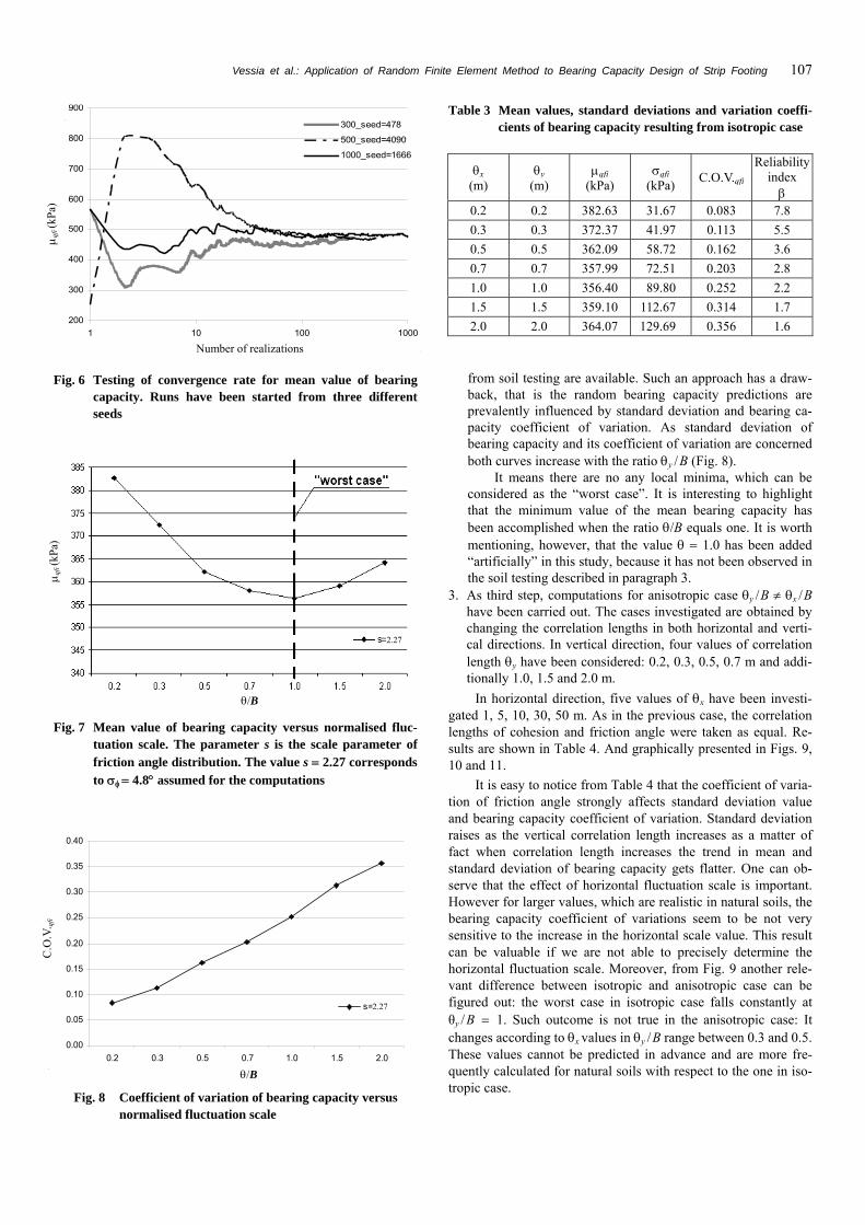
Young’s modulus governs the initial elastic response of the soil, but does not affect the bearing capacity. Thus such elastic soil parameter has been used for pre-analyzing the system. The finite element mesh consists of 1000 elements, 50 elements wide by 20 elements deep (Fig. 5).

Each element is a square of side length 0.1 m and the strip footing occupies 10 elements, thus giving a width of B = 1 m. Since the depth of the model is only 2B some boundary effect can appear. In order to check the correctness of the mesh model an analysis of the mesh influence on the bearing capacity mean value has been carried out. The results are shown in Appendix 1. The random fields in this study are generated using the Local Average Subdivision (LAS) method (Fenton and Vanmarcke 1990). Cross-correlation between the two soil property fields (c and φ) is neglected in the present study (see Appendix 2). Nu-merical analyses of the bearing capacity have been carried out according to the following steps:

Fig. 5 Mesh model used in stochastic bearing capacity

predictions (After Griffiths and Fenton 2001)

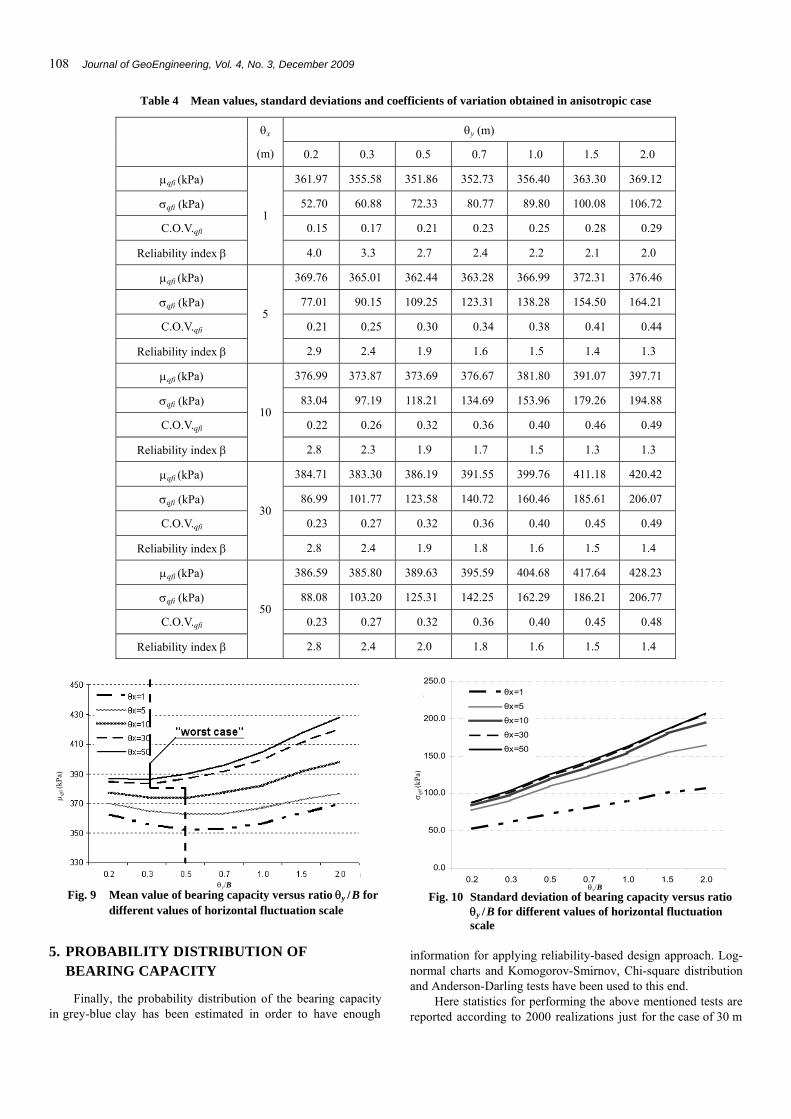
1. At first, the accuracy of the calculation of the first two mo-ments (mean and variance) of the bearing capacity has been assessed. Thus numerical simulations by means of Monte Carlo method were made with a variable number of realiza-tions. Results for 300, 500 and 1000 realizations are reported in Fig. 6. There, the confidence intervals considered with se-lected exceeding probability α = 0.05 are as follows: lower bound of mean value: 450.22 kPa, upper bound of mean value: 481.00 kPa; lower bound of standard deviation: 164.67 kPa, upper bound of standard deviation: 186.46 kPa. Accord-ingly the optimum number of realizations turned out to be 300; whereas more than 1000 realizations are needed to de-termine the approximate form of the bearing capacity distri-bution.

2. At second, the bearing capacity of the system has been calcu-lated for an isotropic case selecting 7 values of fluctuation scale. The values 0.2, 0.3, 0.5, 0.7 m have been reported in the soil testing described in Table 2. Values 1.0, 1.5, 2.0 m have been considered only to catch a trend in the results obtained. According to the assumptions listed in paragraph 3, the corre-lation lengths of cohesion and friction angle were taken equal. Results from numerical computations are reported in Table 3.

The results are also presented graphically in Figs. 7 and 8. It is important to point out that the initial value of the correlation length 0.2 m is comparable with the size of the single element of the mesh (0.1 m). This implies strong averaging of random field fluctuations. As a consequence we may expect inaccuracy with the bearing capacity value in this case. However, the average value, as well as the coefficient of variation of the bearing capacity corresponding to 0.2 m of the correlation length, fit well in with the trend obtained from other results. The isotropic case under consideration (θy / B = θx / B) has shown the so-called “worst case” for mean value. Figure 7 shows the value of normalized fluctuation scale equal to 1 by which the minimal value of bearing capacity appears. Such outcome is in accordance with the observations made in papers by Griffiths and Fenton (2001) and Fenton and Griffiths (2003).

The presence of such minimum value is recognized to be an important information, which allows to determine the “true value” of correlation length even when not enough measure-ments

Dep

th (m

)


200

300

400

500

600

700

800

900

1 10 100 1000Number of realizations

mqf

i

300_seed=478

500_seed=4090

1000_seed=1666

Fig. 6 Testing of convergence rate for mean value of bearing capacity. Runs have been started from three different seeds

Fig. 7 Mean value of bearing capacity versus normalised fluc-tuation scale. The parameter s is the scale parameter of friction angle distribution. The value s = 2.27 corresponds to σφ = 4.8° assumed for the computations

0.00

0.05

0.10

0.15

0.20

0.25

0.30

0.35

0.40

0.2 0.3 0.5 0.7 1.0 1.5 2.0 θ/B

C.O

.V.q

fi

s=2,27

Fig. 8 Coefficient of variation of bearing capacity versus normalised fluctuation scale

Table 3 Mean values, standard deviations and variation coeffi-cients of bearing capacity resulting from isotropic case

θx (m)

θy (m)

μqfi (kPa)

σqfi (kPa) C.O.V.qfi

Reliability index

β 0.2 0.2 382.63 31.67 0.083 7.8 0.3 0.3 372.37 41.97 0.113 5.5 0.5 0.5 362.09 58.72 0.162 3.6 0.7 0.7 357.99 72.51 0.203 2.8 1.0 1.0 356.40 89.80 0.252 2.2 1.5 1.5 359.10 112.67 0.314 1.7 2.0 2.0 364.07 129.69 0.356 1.6

from soil testing are available. Such an approach has a draw-back, that is the random bearing capacity predictions are prevalently influenced by standard deviation and bearing ca-pacity coefficient of variation. As standard deviation of bearing capacity and its coefficient of variation are concerned both curves increase with the ratio θy / B (Fig. 8).

It means there are no any local minima, which can be considered as the “worst case”. It is interesting to highlight that the minimum value of the mean bearing capacity has been accomplished when the ratio θ/B equals one. It is worth mentioning, however, that the value θ = 1.0 has been added “artificially” in this study, because it has not been observed in the soil testing described in paragraph 3.

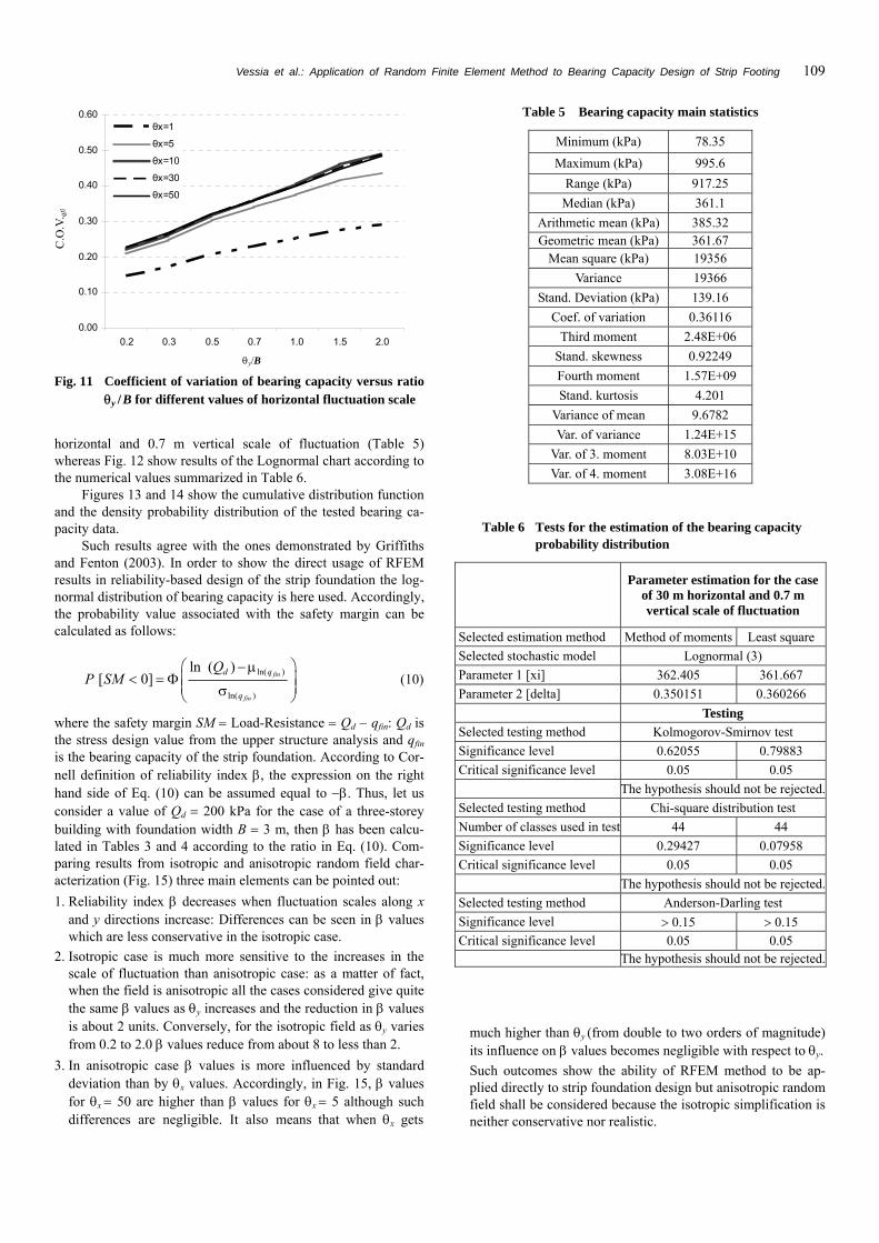
3. As third step, computations for anisotropic case θy / B ≠ θx / B have been carried out. The cases investigated are obtained by changing the correlation lengths in both horizontal and verti-cal directions. In vertical direction, four values of correlation length θy have been considered: 0.2, 0.3, 0.5, 0.7 m and addi-tionally 1.0, 1.5 and 2.0 m.

In horizontal direction, five values of θx have been investi-gated 1, 5, 10, 30, 50 m. As in the previous case, the correlation lengths of cohesion and friction angle were taken as equal. Re-sults are shown in Table 4. And graphically presented in Figs. 9, 10 and 11.

It is easy to notice from Table 4 that the coefficient of varia-tion of friction angle strongly affects standard deviation value and bearing capacity coefficient of variation. Standard deviation raises as the vertical correlation length increases as a matter of fact when correlation length increases the trend in mean and standard deviation of bearing capacity gets flatter. One can ob-serve that the effect of horizontal fluctuation scale is important. However for larger values, which are realistic in natural soils, the bearing capacity coefficient of variations seem to be not very sensitive to the increase in the horizontal scale value. This result can be valuable if we are not able to precisely determine the horizontal fluctuation scale. Moreover, from Fig. 9 another rele-vant difference between isotropic and anisotropic case can be figured out: the worst case in isotropic case falls constantly at θy / B = 1. Such outcome is not true in the anisotropic case: It changes according to θx values in θy / B range between 0.3 and 0.5. These values cannot be predicted in advance and are more fre-quently calculated for natural soils with respect to the one in iso-tropic case.

μ qfi

(kPa

)

Number of realizations

μ qfi

(kPa

)

θ/B

θ/B

C.O

.V. qf

i

2.27

2.27


Table 4 Mean values, standard deviations and coefficients of variation obtained in anisotropic case

θy (m)

θx

(m) 0.2 0.3 0.5 0.7 1.0 1.5 2.0

μqfi (kPa) 361.97 355.58 351.86 352.73 356.40 363.30 369.12

σqfi (kPa) 52.70 60.88 72.33 80.77 89.80 100.08 106.72

C.O.V.qfi 0.15 0.17 0.21 0.23 0.25 0.28 0.29

Reliability index β

1

4.0 3.3 2.7 2.4 2.2 2.1 2.0

μqfi (kPa) 369.76 365.01 362.44 363.28 366.99 372.31 376.46

σqfi (kPa) 77.01 90.15 109.25 123.31 138.28 154.50 164.21

C.O.V.qfi 0.21 0.25 0.30 0.34 0.38 0.41 0.44


5

2.9 2.4 1.9 1.6 1.5 1.4 1.3

μqfi (kPa) 376.99 373.87 373.69 376.67 381.80 391.07 397.71

σqfi (kPa) 83.04 97.19 118.21 134.69 153.96 179.26 194.88

C.O.V.qfi 0.22 0.26 0.32 0.36 0.40 0.46 0.49


10

2.8 2.3 1.9 1.7 1.5 1.3 1.3

μqfi (kPa) 384.71 383.30 386.19 391.55 399.76 411.18 420.42

σqfi (kPa) 86.99 101.77 123.58 140.72 160.46 185.61 206.07

C.O.V.qfi 0.23 0.27 0.32 0.36 0.40 0.45 0.49


30

2.8 2.4 1.9 1.8 1.6 1.5 1.4

μqfi (kPa) 386.59 385.80 389.63 395.59 404.68 417.64 428.23

σqfi (kPa) 88.08 103.20 125.31 142.25 162.29 186.21 206.77

C.O.V.qfi 0.23 0.27 0.32 0.36 0.40 0.45 0.48


50

2.8 2.4 2.0 1.8 1.6 1.5 1.4

Fig. 9 Mean value of bearing capacity versus ratio θy / B for

different values of horizontal fluctuation scale

5. PROBABILITY DISTRIBUTION OF BEARING CAPACITY

Finally, the probability distribution of the bearing capacity in grey-blue clay has been estimated in order to have enough

0.0

50.0

100.0

150.0

200.0

250.0

0.2 0.3 0.5 0.7 1.0 1.5 2.0 θy/B

σqfi θx=1

θx=5

θx=10

θx=30

θx=50

Fig. 10 Standard deviation of bearing capacity versus ratio

θy / B for different values of horizontal fluctuation scale

information for applying reliability-based design approach. Log-normal charts and Komogorov-Smirnov, Chi-square distribution and Anderson-Darling tests have been used to this end.

Here statistics for performing the above mentioned tests are reported according to 2000 realizations just for the case of 30 m

μ qfi

(kPa

)

θy/B

σ qfi

(kPa

)

θy/B


0.00

0.10

0.20

0.30

0.40

0.50

0.60

0.2 0.3 0.5 0.7 1.0 1.5 2.0θy/B

C.O

.V.q

fi θx=1

θx=5

θx=10

θx=30

θx=50

Fig. 11 Coefficient of variation of bearing capacity versus ratio

θy / B for different values of horizontal fluctuation scale

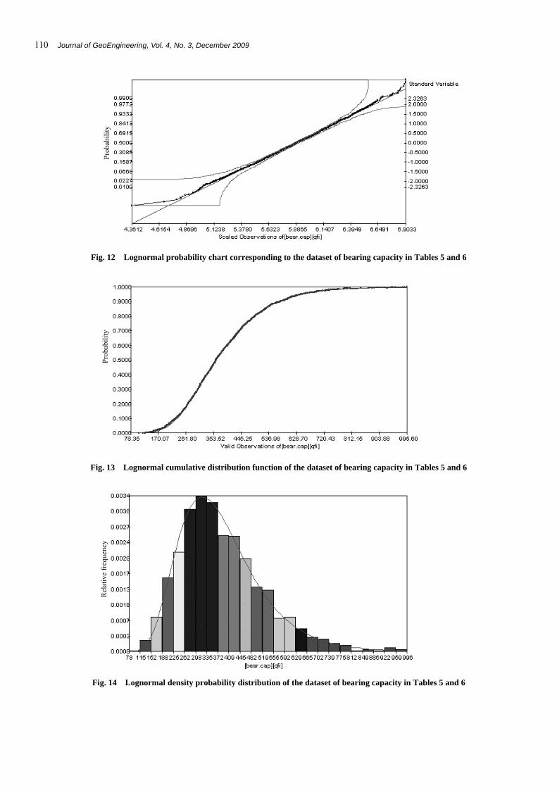
horizontal and 0.7 m vertical scale of fluctuation (Table 5) whereas Fig. 12 show results of the Lognormal chart according to the numerical values summarized in Table 6.

Figures 13 and 14 show the cumulative distribution function and the density probability distribution of the tested bearing ca-pacity data.

Such results agree with the ones demonstrated by Griffiths and Fenton (2003). In order to show the direct usage of RFEM results in reliability-based design of the strip foundation the log-normal distribution of bearing capacity is here used. Accordingly, the probability value associated with the safety margin can be calculated as follows:

ln( )

ln( )

ln ( ) [ 0] fin

fin

d q

q

QP SM

⎛ ⎞− μ< = Φ ⎜ ⎟⎜ ⎟σ⎝ ⎠

(10)

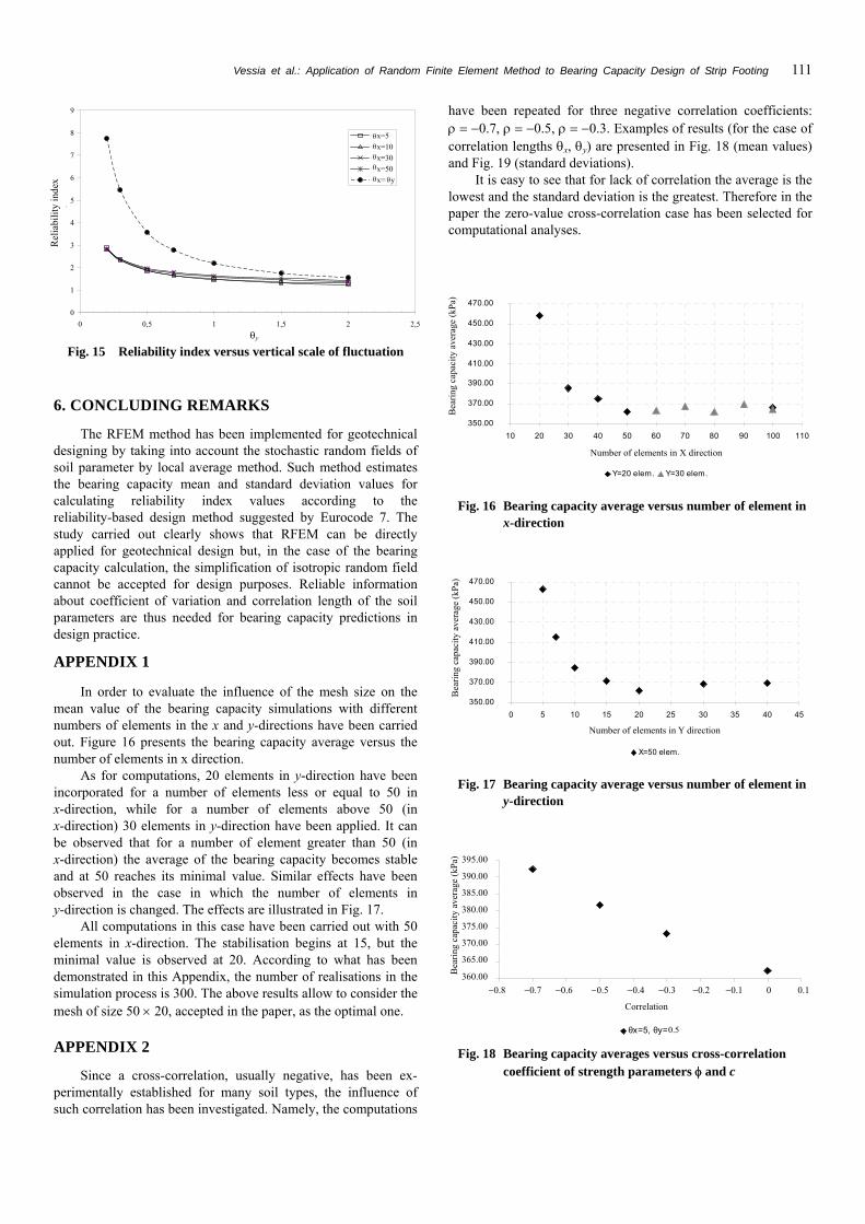
where the safety margin SM = Load-Resistance = Qd − qfin: Qd is the stress design value from the upper structure analysis and qfin is the bearing capacity of the strip foundation. According to Cor-nell definition of reliability index β, the expression on the right hand side of Eq. (10) can be assumed equal to −β. Thus, let us consider a value of Qd = 200 kPa for the case of a three-storey building with foundation width B = 3 m, then β has been calcu-lated in Tables 3 and 4 according to the ratio in Eq. (10). Com-paring results from isotropic and anisotropic random field char-acterization (Fig. 15) three main elements can be pointed out: 1. Reliability index β decreases when fluctuation scales along x

and y directions increase: Differences can be seen in β values which are less conservative in the isotropic case.

2. Isotropic case is much more sensitive to the increases in the scale of fluctuation than anisotropic case: as a matter of fact, when the field is anisotropic all the cases considered give quite the same β values as θy increases and the reduction in β values is about 2 units. Conversely, for the isotropic field as θy varies from 0.2 to 2.0 β values reduce from about 8 to less than 2.

3. In anisotropic case β values is more influenced by standard deviation than by θx values. Accordingly, in Fig. 15, β values for θx = 50 are higher than β values for θx = 5 although such differences are negligible. It also means that when θx gets

Table 5 Bearing capacity main statistics

Minimum (kPa) 78.35 Maximum (kPa) 995.6

Range (kPa) 917.25 Median (kPa) 361.1

Arithmetic mean (kPa) 385.32 Geometric mean (kPa) 361.67

Mean square (kPa) 19356 Variance 19366

Stand. Deviation (kPa) 139.16 Coef. of variation 0.36116

Third moment 2.48E+06 Stand. skewness 0.92249 Fourth moment 1.57E+09 Stand. kurtosis 4.201

Variance of mean 9.6782 Var. of variance 1.24E+15

Var. of 3. moment 8.03E+10 Var. of 4. moment 3.08E+16

Table 6 Tests for the estimation of the bearing capacity probability distribution

Parameter estimation for the caseof 30 m horizontal and 0.7 m vertical scale of fluctuation

Selected estimation method Method of moments Least squareSelected stochastic model Lognormal (3) Parameter 1 [xi] 362.405 361.667 Parameter 2 [delta] 0.350151 0.360266 Testing Selected testing method Kolmogorov-Smirnov test Significance level 0.62055 0.79883 Critical significance level 0.05 0.05 The hypothesis should not be rejected.Selected testing method Chi-square distribution test Number of classes used in test 44 44 Significance level 0.29427 0.07958 Critical significance level 0.05 0.05 The hypothesis should not be rejected.Selected testing method Anderson-Darling test Significance level > 0.15 > 0.15 Critical significance level 0.05 0.05 The hypothesis should not be rejected.

much higher than θy (from double to two orders of magnitude) its influence on β values becomes negligible with respect to θy. Such outcomes show the ability of RFEM method to be ap-plied directly to strip foundation design but anisotropic random field shall be considered because the isotropic simplification is neither conservative nor realistic.

C.O

.V. qf

i

θy/B


Fig. 12 Lognormal probability chart corresponding to the dataset of bearing capacity in Tables 5 and 6

Fig. 13 Lognormal cumulative distribution function of the dataset of bearing capacity in Tables 5 and 6

Fig. 14 Lognormal density probability distribution of the dataset of bearing capacity in Tables 5 and 6

Prob

abili

ty

Prob

abili

ty

Rel

ativ

e fr

eque

ncy


0

1

2

3

4

5

6

7

8

9

0 0,5 1 1,5 2 2,5θy

Rel

iabi

lity

Inde

x

Θx=5Θx=10Θx=30Θx=50Θx=Θy

Fig. 15 Reliability index versus vertical scale of fluctuation

6. CONCLUDING REMARKS

The RFEM method has been implemented for geotechnical designing by taking into account the stochastic random fields of soil parameter by local average method. Such method estimates the bearing capacity mean and standard deviation values for calculating reliability index values according to the reliability-based design method suggested by Eurocode 7. The study carried out clearly shows that RFEM can be directly applied for geotechnical design but, in the case of the bearing capacity calculation, the simplification of isotropic random field cannot be accepted for design purposes. Reliable information about coefficient of variation and correlation length of the soil parameters are thus needed for bearing capacity predictions in design practice.

APPENDIX 1

In order to evaluate the influence of the mesh size on the mean value of the bearing capacity simulations with different numbers of elements in the x and y-directions have been carried out. Figure 16 presents the bearing capacity average versus the number of elements in x direction.

As for computations, 20 elements in y-direction have been incorporated for a number of elements less or equal to 50 in x-direction, while for a number of elements above 50 (in x-direction) 30 elements in y-direction have been applied. It can be observed that for a number of element greater than 50 (in x-direction) the average of the bearing capacity becomes stable and at 50 reaches its minimal value. Similar effects have been observed in the case in which the number of elements in y-direction is changed. The effects are illustrated in Fig. 17.

All computations in this case have been carried out with 50 elements in x-direction. The stabilisation begins at 15, but the minimal value is observed at 20. According to what has been demonstrated in this Appendix, the number of realisations in the simulation process is 300. The above results allow to consider the mesh of size 50 × 20, accepted in the paper, as the optimal one.

APPENDIX 2

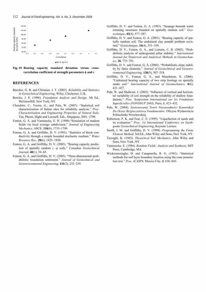
Since a cross-correlation, usually negative, has been ex-perimentally established for many soil types, the influence of such correlation has been investigated. Namely, the computations

have been repeated for three negative correlation coefficients: ρ = −0.7, ρ = −0.5, ρ = −0.3. Examples of results (for the case of correlation lengths θx, θy) are presented in Fig. 18 (mean values) and Fig. 19 (standard deviations).

It is easy to see that for lack of correlation the average is the lowest and the standard deviation is the greatest. Therefore in the paper the zero-value cross-correlation case has been selected for computational analyses.

350.00

370.00

390.00

410.00

430.00

450.00

470.00

10 20 30 40 50 60 70 80 90 100 110

number of elements in X directionB

earin

g C

apac

ity A

vera

ge

Y=20 elem. Y=30 elem.

Fig. 16 Bearing capacity average versus number of element in x-direction

350.00

370.00

390.00

410.00

430.00

450.00

470.00

0 5 10 15 20 25 30 35 40 45

number of elements in Y direction

Bea

ring

Cap

acity

Ave

rage

X=50 elem.

Fig. 17 Bearing capacity average versus number of element in y-direction

360,00

365,00

370,00

375,00

380,00

385,00

390,00

395,00

-0,8 -0,7 -0,6 -0,5 -0,4 -0,3 -0,2 -0,1 0 0,1

correlation

Bear

ing

Capa

city

Ave

rage

θx=5, θy=0,5 Fig. 18 Bearing capacity averages versus cross-correlation

coefficient of strength parameters φ and c

Rel

iabi

lity

inde

x

θy

θθθθ

θ θ

Bea

ring

capa

city

ave

rage

(kPa

) Number of elements in X direction

Bea

ring

capa

city

ave

rage

(kPa

)

Number of elements in Y direction

0.5

Bea

ring

capa

city

ave

rage

(kPa

) 395.00

390.00

385.00

380.00

375.00

370.00

365.00

360.00−0.8 −0.7 −0.6 −0.5 −0.4 −0.3 −0.2 −0.1 0 0.1

Correlation


60,00

70,00

80,00

90,00

100,00

110,00

120,00

-0,8 -0,7 -0,6 -0,5 -0,4 -0,3 -0,2 -0,1 0 0,1

correlation

Bea

ring

Cap

acity

Sta

ndar

d D

evia

tion

θx=5, θy=0,5. Fig. 19 Bearing capacity standard deviation versus cross-

correlation coefficient of strength parameters φ and c

REFERENCES

Baecher, G. B. and Christian, J. T. (2003). Reliability and Statistics in Geotechnical Engineering, Wiley, Chichester, U.K.

Bowles, J. E. (1996). Foundation Analysis and Design, 5th Ed., McGrawHill, New York, NY.

Cherubini, C., Vessia, G., and Pula, W. (2007). “Statistical soil characterization of Italian sites for reliability analysis.” Proc. Characterization and Engineering Properties of Natural Soils, Tan, Phoon, Hight and Lerouell, Eds., Singapore, 2681−2706.

Fenton, G. A. and Vanmarcke, E. H. (1990).“Simulation of random fields via local average subdivision.” Journal of Engineering Mechanics, ASCE, 116(8), 1733−1749.

Fenton, G. A. and Griffiths, D. V. (1993). “Statistics of block con-ductivity through a simple bounded stochastic medium.” Water Resource Res., 29(6), 1825−1830.

Fenton, G. A. and Griffiths, D. V. (2003). “Bearing capacity predic-tion of spatially random c - ϕ soils.” Canadian Geotechnical Journal, 40(1), 54−65.

Fenton, G. A. and Griffiths, D. V. (2005). “Three-dimensional prob-abilistic foundation settlement.” Journal of Geotechnical and Geoenvironmental Engineering, 131(2), 232−239.

Griffiths, D. V. and Fenton, G. A. (1993). “Seepage beneath water retaining structures founded on spatially random soil.” Geo-technique, 43(4), 577−587.

Griffiths, D. V. and Fenton, G. A. (2001). “Bearing capacity of spa-tially random soil: The undrained clay prandtl problem revis-ited.” Geotechnique, 54(4), 351−359.

Griffiths, D. V., Fenton, G. A., and Lemons, C. B. (2002). “Prob-abilistic analysis of underground pillar stability.” International Journal for Numerical and Analytical Methods in Geomechan-ics, 26, 775−791.

Griffiths, D. V. and Fenton, G. A. (2004). “Probabilistic slope stabil-ity by finite elements.” Journal of Geotechnical and Geoenvi-ronmental Engineering, 130(5), 507−518.

Griffiths, D. V., Fenton, G. A., and Manoharan, N. (2006). “Undrained bearing capacity of two strip footings on spatially rando soil.” International Journal of Geomechanics, 6(6), 421−427.

Puła, W. and Shahrour, I. (2003). “Influence of vertical and horizon-tal variability of soil strength on the reliability of shallow foun-dations.” Proc. Symposium International sur les Fondations Superficielles (FONDSUP 2003), Paris, 1, 423−432.

Puła, W. (2004). Zastosowania Teorii Niezawodności Konstrukcji Do Oceny Bezpieczeństwa Fundamentów. Oficyna Wydawnicza Politechniki Wrocławskiej.

Robertson, P. K. and Fear, C. E. (1995). “Liquefaction of sands and its evaluation.” Proc. 1st International Conference on Earth-quake Geotechnical Engineering, Keynote Lecture.

Smith, I. M. and Griffiths, D. V. (1998). Programming the Finite Element Method, 3rd Ed., John Wiley and Sons, New York, NY.

Terzaghi, K. (1943). Theoretical Soil Mechanics, John Wiley and Sons, New York, NY.

Vanmarcke, E. (1984). Random Fields: Analysis and Synthesis, MIT Press, Cambridge, MA.

Wickremesinghe, D. and Campanella, R. G. (1991). “Statistical methods for soil layer boundary location using the cone penetra-tion test.” Proc. ICASP6, Mexico City, 2, 636−643.

Correlation

0.5

Bea

ring

capa

city

stan

dard

de

viat

ion

(kPa

)

120.00

110.00

100.00

90.00

80.00

70.00

60.00−0.8 −0.7 −0.6 −0.5 −0.4 −0.3 −0.2 −0.1 0 0.1

Documents

APPLICATION OF RANDOM FINITE ELEMENT METHOD TO BEARING CAPACITY DESIGN OF STRIP FOOTING