Flux through a Möbius strip?

European Journal of Physics

Eur. J. Phys. 42 (2021) 065804 (12pp) https://doi.org/10.1088/1361-6404/ac1e79

Flux through a Möbius strip?

L Fernández-Jambrina

Matemática e Informática Aplicadas, E.T.S.I, Navales, Universidad Politecnica deMadrid, Avenida de la Memoria 4, E-28040 Madrid, Spain

E-mail: [email protected]

Received 29 May 2021, revised 22 July 2021Accepted for publication 17 August 2021Published 6 September 2021

AbstractIntegral theorems such as Stokes’ and Gauss’ are fundamental in many partsof physics. For instance, Faraday’s law allows computing the induced electriccurrent on a closed circuit in terms of the variation of the flux of a magnetic fieldacross the surface spanned by the circuit. The key point for applying Stokes’theorem is that this surface must be orientable. Many students wonder whathappens to the flux through a surface when this is not orientable, as it happenswith a Möbius strip. On an orientable surface one can compute the flux of asolenoidal field using Stokes’ theorem in terms of the circulation of the vectorpotential of the field along the oriented boundary of the surface. But this cannotbe done if the surface is not orientable, though in principle this quantity couldbe measured on a laboratory. For instance, checking the induced electric currenton a circuit along the boundary of a surface if the field is a variable magneticfield. We shall see that the answer to this puzzle is simple and the problem liesin the question rather than in the answer.

Keywords: Stokes theorem, Moebius strip, Faraday’s law, flux, circulation

1. Introduction

The Möbius strip [1] has attracted the interest of researchers and academics due to its fasci-nating geometric properties [2]. In spite of its name [3], it was not discovered first by AugustFerdinand Möbius, but independently by Johann Benedict Listing [4], the father of moderntopology.

The construction is fairly simple: starting with a rectangular piece of paper, one can jointwo opposite edges in order to form a cylinder. But if before joining the opposite edges wetwist the rectangle 180o we obtain this reknowned one-sided surface.

The strip is a non-orientable surface and for this reason it does not have an outer and an innerside as usual surfaces, such as the sphere, the plane or the cylinder. It is a one-sided surfaceand this fact has suggested many applications in engineering [2]. For instance, for designingaudio and film tapes which could record longer, since they could be used on the only, but

0143-0807/21/065804+12$33.00 © 2021 European Physical Society Printed in the UK 1

https://doi.org/10.1088/1361-6404/ac1e79

https://orcid.org/0000-0002-4872-6973

mailto:[email protected]

http://crossmark.crossref.org/dialog/?doi=10.1088/1361-6404/ac1e79&domain=pdf&date_stamp=2021-9-6

Eur. J. Phys. 42 (2021) 065804 L Fernández-Jambrina

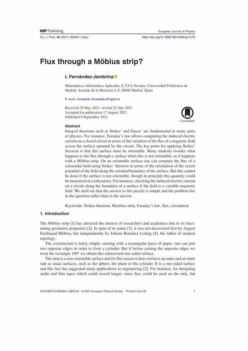
Figure 1. Stokes’ theorem: we have a surface S with unitary normal ν, bounded by aclosed curve Γ with tangent field τ . We may compute the flux of the vector field curl veither by summing up the contributions of 〈curl v, ν〉 on the surface S or the contributionsof 〈v, τ〉 along the curve Γ.

double length, side. For the same reason, it has been used in printing tapes for printers andold typewriters. There are also Möbius’ strips in luggage conveyor belts in airports in orderto double their useful life. And a resistor with this shape was patented [5, 6], made up oftwo conductive layers and filled with a dielectric material, preventing residual self-inductance.There are even aromatic molecules in organic chemistry with this shape [7]. And we cannotforget that it is part of the universal recycling symbol, formed by three green arrows.

But besides academics and engineers, the Möbius strip has attracted the attention of manyscience students. Just check for ‘flux across a Möbius strip’ and you will obtain thousands ofresults in your favourite search engine. We focus on their interest in this issue as target for thispaper, as well as their teachers’.

The reason for this is that integral theorems such as Stokes’ just can be applied to orientablesurfaces [8], relating the flux of the curl of a vector field across a surface with its circulationalong the boundary of the surface (see figure 1).

One might think this is a tricky question, since the answer is negative: it just cannot becalculated. But there are experiments in physics where one could think this question couldhave a meaning.

Consider for instance a circuit attached to the boundary of a Möbius strip. According toFaraday’s law, the flux of a variable magnetic field across the surface induces an electric currenton the circuit. One can measure the electromotive force on the circuit, but in principle Faraday’slaw cannot be applied to calculate it with the flux across the surface. This is the issue we wouldlike to clarify in this paper.

But before providing a solution to this puzzle, we need to recall some useful concepts. Insection 2 we review the concepts of flux and circulation before stating Stokes’ theorem. Insection 3 we describe the Möbius strip as a non-orientable surface. As it was expected, thecalculations performed on the Möbius strip and on its boundary do not coincide, as Stokes’theorem is not applicable, as we show in section 4. But a simple solution to this issue is providedin section 5. A final section of conclusions is included at the end of the paper.

2


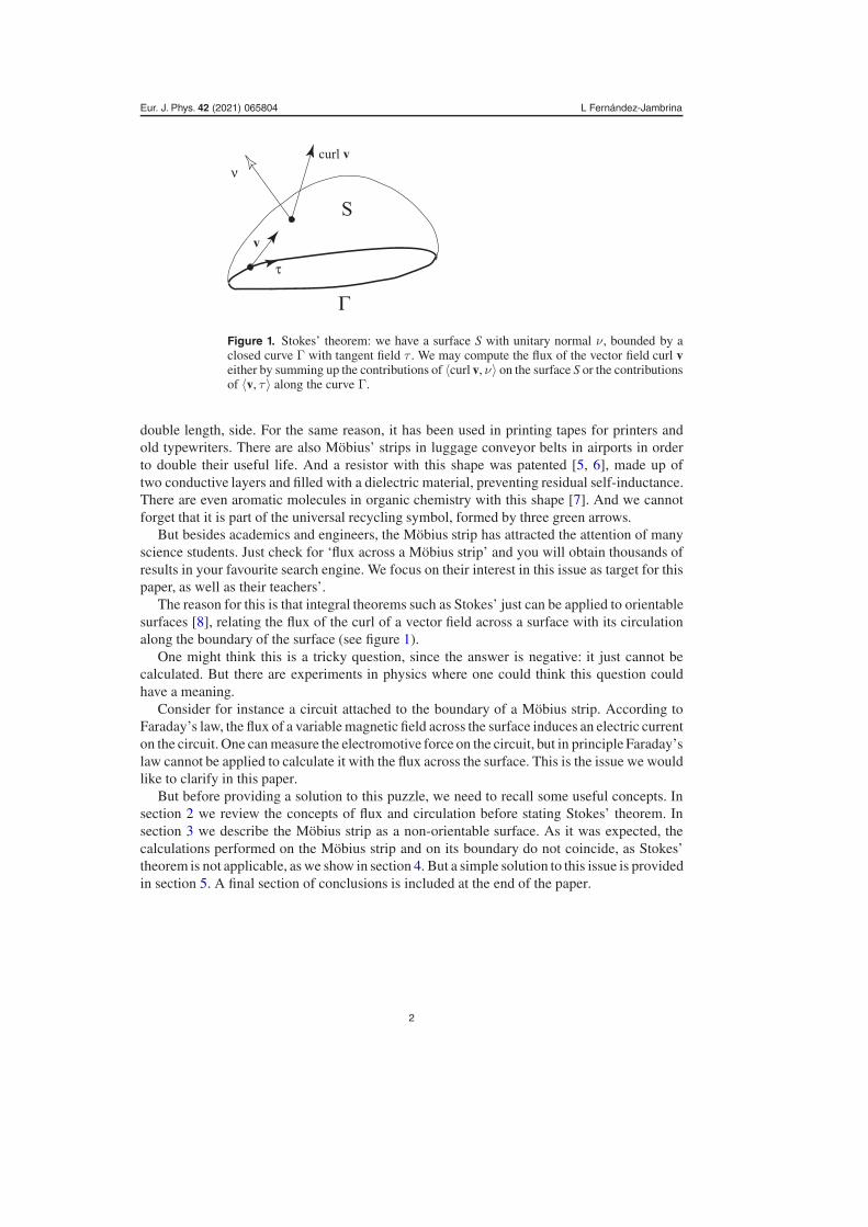
Figure 2. Circulation of the vector field v along the curve Γ: the circulation of thefield v along the curve Γ is calculated summing up the contributions of 〈v, τ〉 along thecurve Γ.

2. Stokes’ theorem

Before recalling Stokes’ theorem, there are a few definitions we need to recall: the circulation ofa vector field along a curve and the flux of a vector field across a surface. This can be reviewedin your favourite Vector Calculus book. I have chosen [8] for its nice examples relating physicsand mathematics.

The line integral or circulation of a vector field along a curve is the generalisation of theconcept of the work done by a force along a trajectory.

Let us consider a continuous vector field v and a curve Γ oriented by its tangent fieldof velocities τ : that is, we specify if the curve is followed onwards or backwards. If thepoints on the curve Γ are parameterised by γ(t) = (x(t), y(t), z(t)), t ∈ [a, b], the velocity ofthis parameterisation is given by τ (γ(t)) = γ ′(t), where the ′ denotes derivation with respect totime t.

We define the line integral or circulation of v along Γ as the sum of the projections of valong τ at the points on the curve,

Cv,Γ :=∫Γ

⟨v,

τ

‖τ‖

⟩ds =

∫ b

a〈v, τ〉γ(t) dt, (1)

taking into account that the length element of a parameterised curve is ds = ‖γ′(t)‖dt. The 〈, 〉stands for the scalar or inner product, whereas ‖‖ stands for the length of a vector.

We see that this definition does not change on changing the parameterisation of the curve,but it depends on the orientation of the curve. That is, it is the same no matter how fast wefollow the curve. But if we follow the curve the other way round, the circulation changes bya sign (see figure 2).

On the other hand, the flux integral of a vector field across a surface is also suggested byexamples in Mechanics, Electromagnetism and Fluid Mechanics [9]: the flux of a gravitationalfield across a closed surface is related to the mass contained inside, the flux of a electrostaticfield is related to the total charge inside the surface and the variation of the flux of a magneticfield across a surface is related to the electromotive force induced on the boundary of thesurface.

Let us consider a compact surface S and a continuous vector field v. The orientation of thesurface is given by a continuous unitary vector field ν normal to S at every point. For a closedsurface, we have just two choices: a vector field pointing inwards or outwards. If such a vector

3


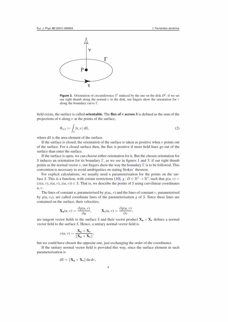
Figure 3. Orientation of circumference S1 induced by the one on the disk D2: if we setour right thumb along the normal ν to the disk, our fingers show the orientation for τalong the boundary curve Γ.

field exists, the surface is called orientable. The flux of v across S is defined as the sum of theprojections of v along ν at the points of the surface,

Φv,S :=∫

S〈v, ν〉 dS, (2)

where dS is the area element of the surface.If the surface is closed, the orientation of the surface is taken as positive when ν points out

of the surface. For a closed surface then, the flux is positive if more field lines go out of thesurface than enter the surface.

If the surface is open, we can choose either orientation for it. But the chosen orientation forS induces an orientation for its boundary Γ, as we see in figures 1 and 3: if our right thumbpoints as the normal vector ν, our fingers show the way the boundary Γ is to be followed. Thisconvention is necessary to avoid amibiguities on stating Stokes’ theorem.

For explicit calculations, we usually need a parameterisation for the points on the sur-face S. This is a function, with certain restrictions [10], g : D ∈ R

2 → R3, such that g(u, v) =

(x(u, v), y(u, v), z(u, v)) ∈ S. That is, we describe the points of S using curvilinear coordinatesu, v.

The lines of constant u, parameterised by g(u0, v) and the lines of constant v, parameterisedby g(u, v0), are called coordinate lines of the parameterisation g of S. Since these lines arecontained on the surface, their velocities,

Xu(u, v) =∂g(u, v)

∂u, Xv(u, v) =

∂g(u, v)∂v

,

are tangent vector fields to the surface S and their vector product Xu × Xv defines a normalvector field to the surface S. Hence, a unitary normal vector field is

ν(u, v) =Xu × Xv

‖Xu × Xv‖,

but we could have chosen the opposite one, just exchanging the order of the coordinates.If the unitary normal vector field is provided this way, since the surface element in such

parameterisation is

dS = ‖Xu × Xv‖ du dv,

4


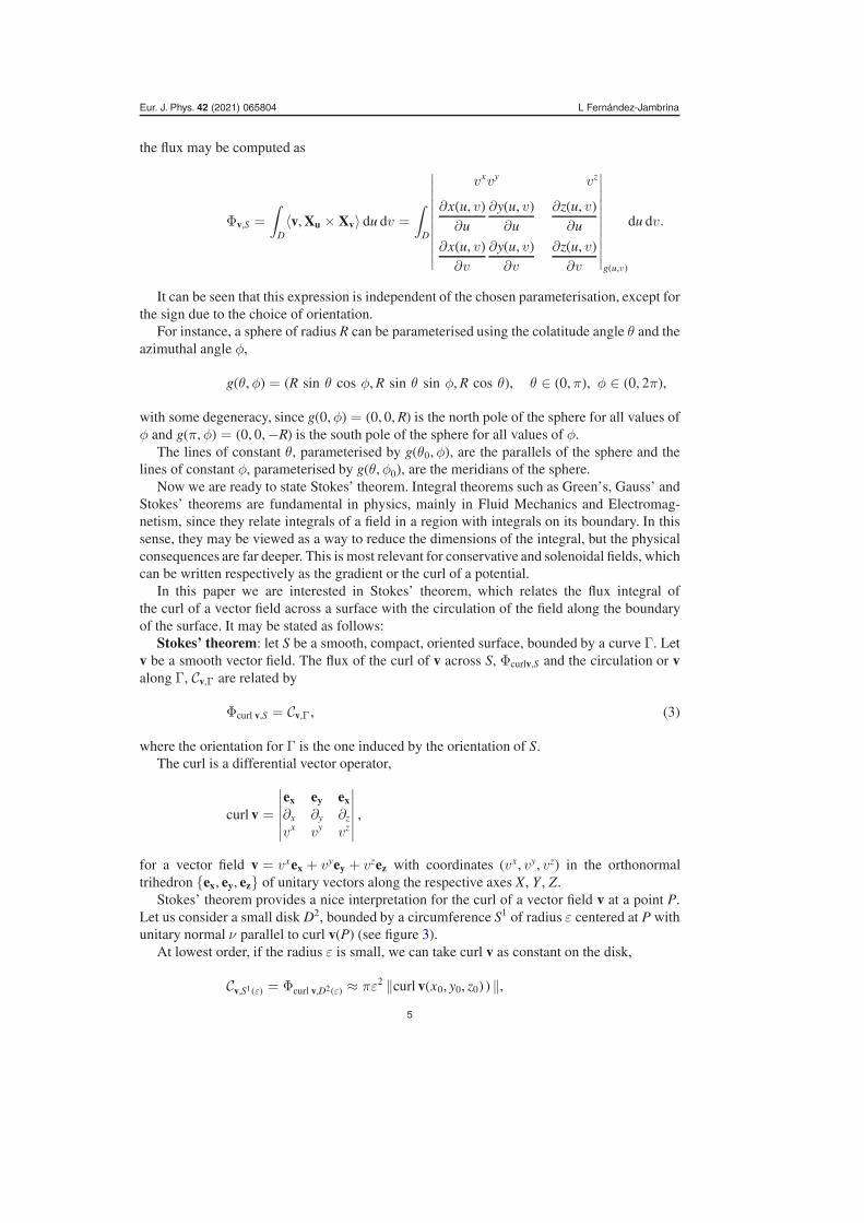
the flux may be computed as

Φv,S =

∫D〈v, Xu × Xv〉 du dv =

∫D

∣∣∣∣∣∣∣∣∣∣∣

vxvy vz

∂x(u, v)∂u

∂y(u, v)∂u

∂z(u, v)∂u

∂x(u, v)∂v

∂y(u, v)∂v

∂z(u, v)∂v

∣∣∣∣∣∣∣∣∣∣∣g(u,v)

du dv.

It can be seen that this expression is independent of the chosen parameterisation, except forthe sign due to the choice of orientation.

For instance, a sphere of radius R can be parameterised using the colatitude angle θ and theazimuthal angle φ,

g(θ,φ) = (R sin θ cos φ, R sin θ sin φ, R cos θ), θ ∈ (0, π), φ ∈ (0, 2π),

with some degeneracy, since g(0,φ) = (0, 0, R) is the north pole of the sphere for all values ofφ and g(π,φ) = (0, 0,−R) is the south pole of the sphere for all values of φ.

The lines of constant θ, parameterised by g(θ0,φ), are the parallels of the sphere and thelines of constant φ, parameterised by g(θ,φ0), are the meridians of the sphere.

Now we are ready to state Stokes’ theorem. Integral theorems such as Green’s, Gauss’ andStokes’ theorems are fundamental in physics, mainly in Fluid Mechanics and Electromag-netism, since they relate integrals of a field in a region with integrals on its boundary. In thissense, they may be viewed as a way to reduce the dimensions of the integral, but the physicalconsequences are far deeper. This is most relevant for conservative and solenoidal fields, whichcan be written respectively as the gradient or the curl of a potential.

In this paper we are interested in Stokes’ theorem, which relates the flux integral ofthe curl of a vector field across a surface with the circulation of the field along the boundaryof the surface. It may be stated as follows:

Stokes’ theorem: let S be a smooth, compact, oriented surface, bounded by a curve Γ. Letv be a smooth vector field. The flux of the curl of v across S, Φcurlv,S and the circulation or valong Γ, Cv,Γ are related by

Φcurl v,S = Cv,Γ, (3)

where the orientation for Γ is the one induced by the orientation of S.The curl is a differential vector operator,

curl v =

∣∣∣∣∣∣ex ey ex

∂x ∂y ∂z

vx vy vz

∣∣∣∣∣∣ ,

for a vector field v = vxex + vyey + vzez with coordinates (vx, vy, vz) in the orthonormaltrihedron {ex, ey, ez} of unitary vectors along the respective axes X, Y , Z.

Stokes’ theorem provides a nice interpretation for the curl of a vector field v at a point P.Let us consider a small disk D2, bounded by a circumference S1 of radius ε centered at P withunitary normal ν parallel to curl v(P) (see figure 3).

At lowest order, if the radius ε is small, we can take curl v as constant on the disk,

Cv,S1(ε) = Φcurl v,D2(ε) ≈ πε2 ‖curl v(x0, y0, z0) ) ‖,

5


and so we may view the curl of v at a point P as the density of circulation of this field on theorthogonal plane, since

‖curl v(P) ) ‖ = limε→0

Cv,S1(ε)

πε2.

Hence, the curl of a field shows the existence of closed field lines or whirlpools (finitecirculation) around a point. Besides, its direction provides the orientation of these whirlpools.This is related to the fact that solenoidal fields are generated by currents instead of charges.

One typical example of application of Stokes’ theorem is Faraday’s law, one of Maxwell’slaws for Electromagnetism [8], which relates the electrical field E with the magnetic field Bthrough

curl E = −∂B∂t

. (4)

If we calculate the circulation of the electric field along a closed curve Γ, after applyingStokes’ theorem to a surface S bounded by Γ, we get

CE,Γ = Φcurl E,S = −Φ ∂B∂t ,S = −∂ΦB,S

∂t,

using Faraday’s law and taking out the derivative with respect to time.If we think of the curve Γ as a closed circuit, the circulation of E is the electromotive force

induced by the varying magnetic field. This is the simple principle which explains how electricmotors work.

Another useful application of the theorem is the calculation of the flux of a solenoidal fieldv = curl A, that is, of a vector field v endowed with a vector potential A,

Φv,S = CA,Γ, (5)

so that it equals the circulation of its vector potential along the boundary of the surface.According to this result, the flux of the solenoidal field v does not depend on the surface

S, but just on its boundary Γ. If the surface is closed, there is no boundary and the flux of asolenoidal field across closed surfaces is always zero. For open surfaces, the flux is the sameacross any other surface bounded by Γ. This fact shall be useful for our purposes later on.

3. Möbius strip

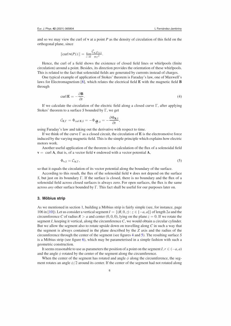
As we mentioned in section 1, building a Möbius strip is fairly simple (see, for instance, page106 in [10]). Let us consider a vertical segment I = {(R, 0, z) : z ∈ [−a, a]} of length 2a and thecircumference C of radius R > a and center (0, 0, 0), lying on the plane z = 0. If we rotate thesegment I, keeping it vertical, along the circumference C, we would obtain a circular cylinder.But we allow the segment also to rotate upside down on travelling along C in such a way thatthe segment is always contained in the plane described by the Z axis and the radius of thecircumference through the center of the segment (see figures 4 and 5). The resulting surface Sis a Möbius strip (see figure 6), which may be parameterised in a simple fashion with such ageometric construction.

It seems reasonable to use as parameters the position of a point on the segment I, r ∈ (−a, a)and the angle φ rotated by the center of the segment along the circumference.

When the center of the segment has rotated and angle φ along the circumference, the seg-ment rotates an angle φ/2 around its center. If the center of the segment had not rotated along

6


Figure 4. Initial location of the segment I and after its center rotates φ = π/2.

Figure 5. Location of the segment I after its center rotates φ = π, 3π/2, 2π.

Figure 6. Möbius strip.

the circumference, it would have been parameterised as (R + r sin(φ/2), 0, r cos(φ/2)). Butsince it has rotated an angle φ along the circumference, we have

7


g(r,φ) =

((R + r sin

φ

2

)cos φ,

(R + r sin

φ

2

)sin φ, r cos

φ

2

),

for r ∈ (−a, a), φ ∈ (0, 2π) as a parameterisation for the Möbius’ strip.That is, g(r,φ) describes the position of the original point corresponding to r ∈ (−a, a) after

rotation of the segment by an angle φ/2 and rotation of its center along the circumference byan angle φ.

Using the velocities of the coordinate lines,

Xr(r,φ) =

(sin

φ

2cos φ, sin

φ

2sin φ, cos

φ

2

),

Xφ(r,φ) =

(−(

R + r sinφ

2

)sin φ,

(R + r sin

φ

2

)cos φ, 0

)

+12

(r cos

φ

2cos φ, r cos

φ

2sin φ,−r sin

φ

2

),

we may obtain a normal vector field, Xr × Xφ to the strip at every point.We notice that this normal vector field is not continuous: if we compare the expressions at

the center of the segment, r = 0, after completing a turn from φ = 0 to φ = 2π,

N(0, 0) = (0, 0, 1)× (0, R, 0) = (−R, 0, 0),

N(0, 2π) = (0, 0,−1)× (0, R, 0) = (R, 0, 0),

the normal vector changes from pointing out of the center of the circumference to pointingtowards the center, though the point on the strip is the same. Hence, the Möbius strip is notorientable.

The boundary Γ of the Möbius strip S is the curve described by both endpoints {−a, a} ofthe segment on rotating. Or equivalently, since the endpoint a arrives at the original positionof −a after a whole turn, we may describe Γ by the motion of just the endpoint a after thesegment travels twice along the circumference to end up at the original position,

γ(φ) =

((R + a sin

φ

2

)cos φ,

(R + a sin

φ

2

)sin φ, a cos

φ

2

),

for φ ∈ [0, 4π].

4. Flux across a Möbius’ strip

We are ready to perform some calculations on the strip and its boundary. For simplicity, weconsider a simple constant vector field along the Z axis, v = (0, 0, 1). This field is solenoidaland a simple vector potential for it is A(x, y, z) = (−y/2, x/2, 0). That is, v = curl A.

The circulation of A along Γ, the boundary of the strip S is well defined, since it is anoriented curve, and may be readily computed.

We need the velocity of the parameterisation of Γ, with velocity,

γ ′(φ) =

(−(

R + a sinφ

2

)sin φ,

(R + a sin

φ

2

)cos φ, 0

)

+12

(a cos

φ

2cos φ, a cos

φ

2sin φ,−a sin

φ

2

),

8


and the vector potential on the points of Γ in this parameterisation,

A(x(r,φ), y(r,φ), z(r,φ)) =12

(−(

R + a sinφ

2

)sin φ,

(R + a sin

φ

2

)cos φ, 0

).

Their inner product is just

〈A(γ (φ)), γ ′(φ)〉 = 12

(R + a sin

φ

2

)2

,

which makes the calculation of the circulation simple,

CA,Γ =

∫ 4π

0〈A(γ(φ)), γ ′(φ)〉 dφ =

12

∫ 4π

0

(R + a sin

φ

2

)2

dφ = 2πR2 + πa2.

(6)

But if we naively calculate the flux of v across the strip,

Φv,S =

∫ a

−adr∫ 2π

0dφ 〈v, Xr × Xφ〉 =

∫ a

−adr∫ 2π

0dφ

(R + r sin

φ

2

)sin

φ

2

= 8Ra,

which of course does not provide the same result as the circulation of A along the boundary Γ,since the strip is not orientable and Stokes’ theorem is not applicable.

However, there is a way to provide a meaning and an interpretation to the previous integral.If we cut the strip along the original segment at φ = 0, we obtain an oriented open strip, butits boundary is not Γ as one could expect, but the union Γ of four pieces: the piece of Γ corre-sponding to φ ∈ (0, 2π), the piece ofΓ corresponding to φ ∈ (2π, 4π) with reversed orientationand the original segment I counted twice to link both segments of Γ (see figure 7). Since I isorthogonal to A, it does not contribute to the circulation,

CA,Γ =

∫ 2π

0〈A(γ(φ)), γ ′(φ)〉 dφ−

∫ 4π

2π〈A(γ(φ)), γ ′(φ)〉 dφ

=12

∫ 2π

0

(R + a sin

φ

2

)2

dφ− 12

∫ 4π

2π

(R + a sin

φ

2

)2

dφ = 8Ra,

which of course provides the same result as the flux across the open strip, since Stokes’ theoremis applicable to this oriented surface.

Though of course it is not the result we are after, since we wish to recover the circulationof A along Γ, not the flux of curl A across a broken Möbius strip.

5. Circulation along the boundary of the strip

We have checked explicitly that the flux of a solenoidal field across a Möbius’ strip and thecirculation of its potential vector along the boundary of the strip are not the same, since Stokes’theorem cannot be applied to a non-orientable surface.

9


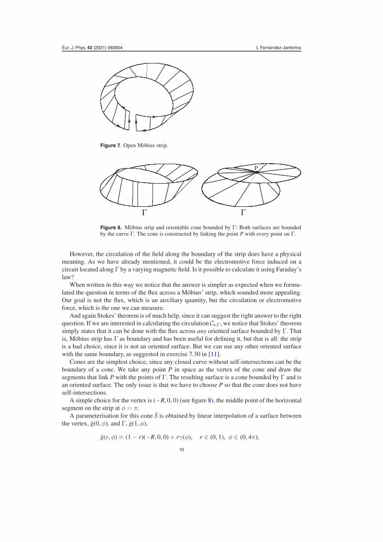
Figure 7. Open Möbius strip.

Figure 8. Möbius strip and orientable cone bounded by Γ: Both surfaces are boundedby the curve Γ. The cone is constructed by linking the point P with every point on Γ.

However, the circulation of the field along the boundary of the strip does have a physicalmeaning. As we have already mentioned, it could be the electromotive force induced on acircuit located along Γ by a varying magnetic field. Is it possible to calculate it using Faraday’slaw?

When written in this way we notice that the answer is simpler as expected when we formu-lated the question in terms of the flux across a Möbius’ strip, which sounded more appealing.Our goal is not the flux, which is an auxiliary quantity, but the circulation or electromotiveforce, which is the one we can measure.

And again Stokes’ theorem is of much help, since it can suggest the right answer to the rightquestion. If we are interested in calculating the circulation Cv,Γ, we notice that Stokes’ theoremsimply states that it can be done with the flux across any oriented surface bounded by Γ. Thatis, Möbius strip has Γ as boundary and has been useful for defining it, but that is all: the stripis a bad choice, since it is not an oriented surface. But we can use any other oriented surfacewith the same boundary, as suggested in exercise 7.30 in [11].

Cones are the simplest choice, since any closed curve without self-intersections can be theboundary of a cone. We take any point P in space as the vertex of the cone and draw thesegments that link P with the points of Γ. The resulting surface is a cone bounded by Γ and isan oriented surface. The only issue is that we have to choose P so that the cone does not haveself-intersections.

A simple choice for the vertex is (−R, 0, 0) (see figure 8), the middle point of the horizontalsegment on the strip at φ = π.

A parameterisation for this cone S is obtained by linear interpolation of a surface betweenthe vertex, g(0,φ), and Γ, g(1,φ),

g(r,φ) = (1 − r)(−R, 0, 0) + rγ(φ), r ∈ (0, 1), φ ∈ (0, 4π),

10


with the corresponding velocities for the coordinate lines,

Xr(r,φ) = γ(φ) − (R, 0, 0), Xφ(r,φ) = rγ ′(φ),

allows calculation of the flux of v across the cone,

Φv,S =

∫ 1

0dr∫ 4π

0dφ 〈v, Xr × Xφ〉

=

∫ 1

0dr∫ 4π

0dφ

(2R2 cos2φ

2+ Ra

(1 + 3 cos2 φ

2

)sin

φ

2+ a2 sin2 φ

2

)r

= 2πR2 + πa2,

and obtain the same results as with the circulation (6), according to Stokes’ theorem, since thecone is orientable.

Calculations provide the same result for any other choice of the vertex P of the cone.

6. Conclusions

In this paper we have provided a simple answer to the calculation of the flux of a vector fieldacross a one-sided surface, where Stokes’ theorem is not applicable.

We have shown that, though the question is ill posed, there is a way of restating the problemin order to provide a right answer, that is related to experiments we may perform in a laboratory.

It has been pointed out that the physically meaningful quantity is not the flux across theone-sided surface, but the circulation along the boundary of the surface. This quantity is notalso meaningful, but can be measured, for instance, as the electromotive force along a circuitinduced by a varying magnetic field.

In fact, once we focus in computing the circulation along the boundary, we notice that theone-sided surface is auxiliary and may be replaced by any other surface with the same bound-ary. If the chosen surface is orientable, this allows us to calculate the flux and the circulationan obtain the same result, according to Stokes’ theorem. In fact, cones are always available fordesigning orientable surfaces with a given closed curve as boundary.

Summarising, the circulation of a vector field along the boundary of a Möbius strip, or anyother one-sided surface, can be calculated using Stokes’ theorem, though not using the Möbiusstrip, but any other surface with the same boundary.

Acknowledgments

This work is partially supported by Protocommunity SSERIES (Science for Sustainable Envi-sion of Reality and Information for an Engaged Society), European Engineering LearningInnovation and Science Alliance (EELISA).

ORCID iDs

L Fernández-Jambrina https://orcid.org/0000-0002-4872-6973

References

[1] Pickover C A 2006 The Möbius Strip (New York: Thunder’s Mouth Press)

11

https://orcid.org/0000-0002-4872-6973

https://orcid.org/0000-0002-4872-6973


[2] Macho M 2008 Las sorprendentes aplicaciones de la banda de Möbius Actas Segundo Con-greso Internacional de Matemáticas en la Ingeniería y la Arquitectura (Madrid: UniversidadPolitecnica de Madrid) pp 29–61

[3] O’Connor J J and Robertson E F 1997 August Ferdinand Möbius MacTutor History of MathematicsArchive (Scotland: University of St Andrews)

[4] O’Connor J J and Robertson E F 2000 Johann Benedict Listing MacTutor History of MathematicsArchive (Scotland: University of St Andrews)

[5] Time 1964 Electronics: Making Resistors with Math vol 84 (New York: Time Warner) http://content.time.com/time/subscriber/article/0,33009,876181,00.html

[6] Davies R 1969 Non-inductive resistor https://rexresearch.com/davis/davis.htm[7] Flapan E 2000 When Topology Meets Chemistry: A Topological Look at Molecular Chirality

(Cambridge: Cambridge University Press)[8] Marsden J E and Tromba A J 2003 Vector Calculus 5th edn (San Francisco, CA: Freeman)[9] Aris R 1989 Vectors, Tensors and the Basic Equations of Fluid Mechanics (New York: Dover)

[10] do Carmo M P 1976 Differential Geometry of Curves and Surfaces (Englewood Cliffs, NJ: Prentice-Hall)

[11] Purcell E M 1985 Electricity and magnetism Berkeley Physics Course 2nd edn (New York: McGraw-Hill)

12

http://content.time.com/time/subscriber/article/0,33009,876181,00.html

http://content.time.com/time/subscriber/article/0,33009,876181,00.html

https://rexresearch.com/davis/davis.htm

Documents

Flux through a Möbius strip?