Analytical model for the performance of the tunnel-type greenhouse drier

Renewable Energy 28 (2003) 467–485www.elsevier.com/locate/renene

Analytical model for the performance of thetunnel-type greenhouse drier

M. Condorı*, L. SaraviaINENCO, Instituto de Investigacio´n en Energı´a no Convencional, Universidad Nacional de Salta,

Calle Buenos Aires 177, 4400 Salta, Argentina

Received 9 November 2000; accepted 12 June 2001

Abstract

An analytical study describing the performance of a tunnel greenhouse drier is presented.Considering the greenhouse as a solar collector, a linear function between the incident solarradiation and the greenhouse output temperature is obtained. Using the drier characteristicfunction, the drier performance is evaluated as a function of the drying potentials. The resultsshow that an almost constant production is obtained each day. The generalized drying curveconcept is applied to the first tunnel cart, obtaining a result that is similar to the single chamberdrier case. The simulation tests with red sweet pepper show an improvement of 160% in theproduction, compared with the single chamber drier case, and an improvement around 40%,if the double chamber drier is considered. 2002 Elsevier Science Ltd. All rights reserved.

1. Introduction

This paper is an analytical study of a recently proposed drier [1]: the tunnel green-house drier. This study is similar to one carried out with other kinds of greenhousedrier, the single and double chamber driers [2], where the main simplifying hypoth-esis was that the chambers had a uniform distribution of temperature and humidity.In this work, the change of the main variables on the position along a drying tunnelis considered.

* Corresponding author. Tel.:+54-387-425-5579; fax:+54-387-425-5489.E-mail address:[email protected] (M. Condorı´).

0960-1481/03/$ - see front matter 2002 Elsevier Science Ltd. All rights reserved.PII: S0960 -1481(01 )00137-9

https://www.researchgate.net/publication/222919816_The_performance_of_forced_convection_greenhouse_driers?el=1_x_8&enrichId=rgreq-c91917c4869b8d5cb7754cd09f1c9815-XXX&enrichSource=Y292ZXJQYWdlOzIyMjM2OTA3MjtBUzoyNjc3ODMzNjc4MTkyNzRAMTQ0MDg1NTkzODIwOA==

https://www.researchgate.net/publication/223209899_Solar_drying_of_sweet_pepper_and_garlic_using_the_tunnel_greenhouse_drier?el=1_x_8&enrichId=rgreq-c91917c4869b8d5cb7754cd09f1c9815-XXX&enrichSource=Y292ZXJQYWdlOzIyMjM2OTA3MjtBUzoyNjc3ODMzNjc4MTkyNzRAMTQ0MDg1NTkzODIwOA==

468 M. Condorı, L. Saravia / Renewable Energy 28 (2003) 467–485

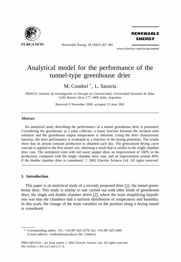
Fig. 1. Working scheme for the tunnel greenhouse drier. Sectional view.

Two working schemes for the tunnel greenhouse drier are shown in Fig. 1 andFig. 2. The drier consists of two main parts: (a) the solar collector and (b) the dryingtunnel. Both of them are integrated under the same greenhouse structure. The dryingtunnel, built with transparent plastic and wood, has a relatively small soil area inthe greenhouse while the remaining surface of the greenhouse works as a solar collec-tor. The fresh product is placed on trays that are stacked on movable carts that runalong the tunnel.

The ambient air is introduced in the greenhouse through two small windows onthe cover and it is heated by convection with the soil. The fans push the air throughthe carts, where it is loaded with vapor delivered by the product. Then, the air leavesthe drier.

The most commonly used greenhouse driers are the batch ones. In these driers,the product remains in the drier for some days. The drying time depends on themoisture content of the product, the exposure area, the initial product load and themeteorological conditions. The available energy is fully used only during the firstday, when the moisture content of the product is still high. In the following days,the drying resistance of the product increases and the air flow leaves the drier with

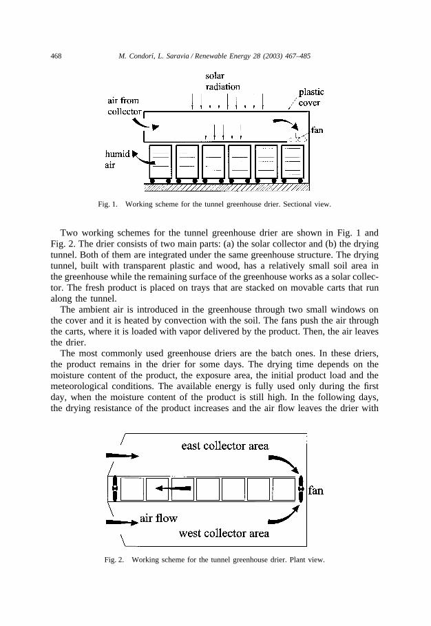
Fig. 2. Working scheme for the tunnel greenhouse drier. Plant view.

469M. Condorı, L. Saravia / Renewable Energy 28 (2003) 467–485

a low humidity and a high temperature; thus, only a small percentage of the incomingsolar energy is used in the drying process.

On the other hand, the tunnel greenhouse drier works continuously, obtaining adaily production. The maximum drying potential of the hot air coming from thecollector area is mainly used in the first carts. Each day, dried product is removedfrom the tunnel, while an equal amount of new fresh product is loaded through itsother end. As the air flows in a reverse sense — relative to the carts — the availableenergy is used efficiently.

Another characteristic feature of this proposed greenhouse drier is that the tunnelreceives direct solar radiation. The product receives solar radiation through the trans-parent walls, increasing its internal temperature and improving the final evapor-ation velocity.

An analytical model for the product-drier system is presented in the followingsections. The solar collector area is analyzed separately from the drying tunnel. How-ever, both behaviors are related given that part of the tunnel heat losses are absorbedby the collector zone.

2. The greenhouse as a collector

In this case, the air coming into the greenhouse is at ambient temperature and thethermal efficiency of the solar collector h only depends on the heat remotion factorFR and of the greenhouse optic parameters [3]

h � FR(ta) (1)

where t is the cover transmittance and a the greenhouse average radiation absorptioncoefficient. According to Eq. (1), the greenhouse works at a unique point of theefficiency curve that corresponds to the intersection of this curve with the ordinateaxis.

The instantaneous efficiency is

h �Cpma(Ts�Ta)

AscI(2)

where I is the total incident solar radiation on horizontal surface, Asc the solar collec-tion surface, Cp the air specific heat capacity, ma the air mass flow, Ts the exit tem-perature in the collector zone, and Ta the ambient temperature.h is constant, since FR and (ta) have no appreciable changes during the process,

and Eq. (2) determines a linear relation between the temperature Ts and the incidentradiation I

Ts � Ta � kI (3)

where the constant k is defined as

k �hAsc

Cpma(4)



Moreover, if a simple global energy balance is performed, the following equationfor the greenhouse is obtained:

(ta)AscI � Cpma(Ts�Ta) � hcAc(Ts�Ta) (5)

where the absorbed solar radiation is distributed between the air heating and thethermal losses to the environment. Ac is the heat losses surface and hc the correspond-ing global losses coefficient. In this balance, a uniform temperature for the collectorzone is considered. The heat stored in the soil is not included, since part of it returnsto the greenhouse in the afternoon and evening hours. From Eq. (5), the relationbetween the temperature Ts and the incident radiation I is determined, obtaininganother expression for the constant k

k �(ta)Asc

Cpma � hcAc

(6)

Eliminating the constant k from Eq. (4) and Eq. (6), the following expressions forthe efficiency and the heat remotion factor are determined:

h �(ta)Cpma

Cpma � hcAc

(7)

FR �1

1 � c(8)

In these equations, both h and FR have a constant behavior with respect to time andonly depend on the greenhouse operative parameters. For the FR case, these para-meters are grouped in a non-dimensional variable: the ratio between the total heatlosses and the sensible heat carried by the air flow

c �hcAc

Cpma(9)

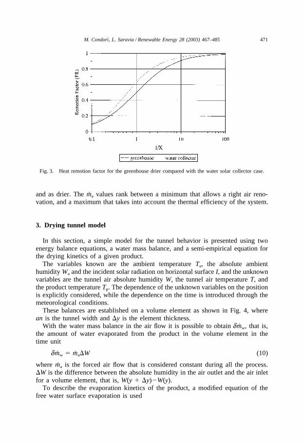
If c � 1, both contributions are equal and FR � 0.5. In greenhouses, typical valuesof c are bigger than 1, producing a low value for the heat remotion factor. Fig. 3shows FR given by Eq. (8) when it is compared with FR corresponding to the watersolar collector [3]. Both have a similar general behavior, being values that correspondto water collector higher since it has better thermal insulation.

According to Eq. (1), it is possible to improve the thermal efficiency of the drierif the following alternatives are adopted, considering constant values for t, hc and Cp:

1. to increase a using materials with a better radiation absorption,2. optimizing c either decreasing the greenhouse dimensions to reduce the cover

heat losses or increasing the air flow.

In the latter case, the air flow is also conditioned by the drying process, since itdetermines the tunnel temperature and the evaporation velocity. To obtain anadequate value for ma it is necessary to optimize the system behavior both as collector


Fig. 3. Heat remotion factor for the greenhouse drier compared with the water solar collector case.

and as drier. The ma values rank between a minimum that allows a right air reno-vation, and a maximum that takes into account the thermal efficiency of the system.

3. Drying tunnel model

In this section, a simple model for the tunnel behavior is presented using twoenergy balance equations, a water mass balance, and a semi-empirical equation forthe drying kinetics of a given product.

The variables known are the ambient temperature Ta, the absolute ambienthumidity Wa and the incident solar radiation on horizontal surface I, and the unknownvariables are the tunnel air absolute humidity W, the tunnel air temperature T, andthe product temperature Tp. The dependence of the unknown variables on the positionis explicitly considered, while the dependence on the time is introduced through themeteorological conditions.

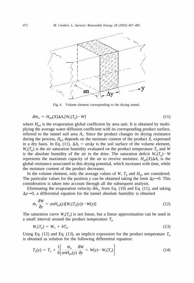
These balances are established on a volume element as shown in Fig. 4, wherean is the tunnel width and �y is the element thickness.

With the water mass balance in the air flow it is possible to obtain dmw, that is,the amount of water evaporated from the product in the volume element in thetime unit

dmw � ma�W (10)

where ma is the forced air flow that is considered constant during all the process.�W is the difference between the absolute humidity in the air outlet and the air inletfor a volume element, that is, W(y � �y)�W(y).

To describe the evaporation kinetics of the product, a modified equation of thefree water surface evaporation is used


Fig. 4. Volume element corresponding to the drying tunnel.

dmw � Hpd(X)�As[Ws(Tp)�W] (11)

where Hpd is the evaporation global coefficient by area unit. It is obtained by multi-plying the average water diffusion coefficient with its corresponding product surface,referred to the tunnel soil area As. Since the product changes its drying resistanceduring the process, Hpd depends on the moisture content of the product X, expressedin a dry basis. In Eq. (11), �As � an�y is the soil surface of the volume element,Ws(Tp) is the air saturation humidity evaluated on the product temperature Tp and Wis the absolute humidity of the air in the drier. The saturation deficit Ws(Tp)�Wrepresents the maximum capacity of the air to receive moisture. Hpd(X)�As is theglobal resistance associated to this drying potential, which increases with time, whilethe moisture content of the product decreases.

In the volume element, only the average values of W, Tp and Hpd are considered.The particular values for the position y can be obtained taking the limit �y→0. Thisconsideration is taken into account through all the subsequent analysis.

Eliminating the evaporation velocity dmw from Eq. (10) and Eq. (11), and taking�y→0, a differential equation for the tunnel absolute humidity is obtained

ma

∂W∂y

� anHpd(y)[Ws(Tp(y))�W(y)] (12)

The saturation curve Ws(Tp) is not linear, but a linear approximation can be used ina small interval around the product temperature Tp

Ws(Tp) � Wo � bTp. (13)

Using Eq. (12) and Eq. (13), an implicit expression for the product temperature Tp

is obtained as solution for the following differential equation:

Tp(y) � Ta �1b� ma

anHpd(y)∂W∂y

� W(y)�Ws(Ta)� (14)


where Ws(Ta) is the proposed linear relation in Eq. (13), evaluated in Ta.The first energy balance is performed on the product. The effective solar radiation

received by the product is spent among the evaporation energy and the convectivelosses toward the air flow. The heat stored in the product is underrated if comparedwith the aforementioned energies.

(tap)2Api�AsI � qfdmw � HpT�As(Tp�T) (15)

where (tap)2 is the cover transmittance — the product average absorption coefficient,Api the exposure area of the product to the solar radiation, referred to As, qf the waterevaporation latent heat and HpT the average convective coefficient multiplied by itscorresponding product surface, also referred to As.

Replacing Eq. (10) in Eq. (15), and taking the limit �y→0, the following implicitdifferential expression for T(y) as a function of Tp and W is obtained:

T(y) � Tp(y) �1

HpT�qf

ma

an∂W∂y

�(tap)2ApiI�. (16)

Furthermore, if the product temperature, given in Eq. (14), is used in Eq. (16), anew implicit differential equation is obtained where only T and W are coupled

T(y) � Ta � B(y)∂W∂y

�1b[W(y)�Ws(Ta)]�(tap)2

Api

HpT

I. (17)

The coefficient B depends on the position y through Hpd

B(y) �ma

an� 1bHpd(y)

�qf

HpT�.

Another global balance of the energy is carried out in the tunnel. The absorbed solarradiation in the tunnel is distributed among the energy used in the evaporation, theheat losses toward the air flow, and the thermal losses toward the collector zone;the latter having a uniform temperature Ts

(ta)1�AsI � Cpma�T � qfdmw � hcAc�As(T�Ts) (18)

where (ta)1 is the cover transmittance — the tunnel average absorption coefficient,Cp the air specific heat, �T the temperature difference between the air outlet and airinlet of the volume element, hc the thermal losses coefficient of the tunnel, and Ac

its corresponding surface, referred to as As. The soil-stored heat is not considered.Combining Eq. (10) and Eq. (18), using Eq. (3), and taking the limit �y→0,

another differential equation for T and W is obtained

Cp

ma

an∂T∂y

� qf

ma

an∂W∂y

� hcAc(T�Ta�kI) � (ta)1I � 0 (19)

The two differential equations, Eq. (17) and Eq. (19), have a unique solution, andit is possible to obtain an explicit differential expression for W(y) using the firstderivative of Eq. (17). In this way, we can obtain the following non-homogeneous-second-order differential equation with variable coefficients


a1(y)∂2W∂y2 � a2(y)

∂W∂y

� a3W � a4 (20)

where

a1(y) �ma

anCpB(y)

a2(y) �ma

an�Cp�∂B∂y

�1b� � qf� � hcAcB(y)

a3 �hcAc

b

a4 � A∗I � a3Ws(Ta)

A∗ � (ta)1 � hcAc�k � (tap)2

Api

HpT�

The constant a4 considers the most important meteorological variables in the process,I and Ta, that only depend on time.

It is possible to solve Eq. (20) using power series if the functions a1(y) and a2(y)are known, but both of them are unknown variables at the initial time.

An easier approach would be to consider the constant coefficients. That is, thewater content of the product is considered constant during a short interval, in whichthe mass and the energy balances are established. Such assumption can only be madefor a small section of the tunnel; however, this section should be long enough sothat its application makes sense. This consideration agrees with the actual situation:the product is distributed in carts and an average behavior is considered for eachone. The error that is introduced in the final result due to the use of this approachcan be bounded by decreasing the section length.

Next, the tunnel is divided into sections, and the problem of constant coefficientis solved for a given section where the boundary conditions are known. This solutionis considered as the boundary condition for the next tunnel section, which containsproduct with a different moisture content.

Considering a tunnel section of longitude �L, where L is the total length of thetunnel and the condition �L��y is accomplished, Eq. (20) is changed into a second-order-homogeneous differential equation with constant coefficients, DECC (21). Per-forming the following change of variables CHV (22):

W∗(y) � W(y)�a4

a3(21)

∂2W∗∂y2 � b1

∂W∗∂y

� b2W∗ � 0 (22)

where


b1 �1B�qf

Cp

�1b� �

anhcAc

maCp

b2 �1B

anhcAc

bmaCp

The characteristic polynomial, associated with Eq. (21) has m1 and m2 as solutions

m1, m2 ��b1 ± �b2

1�4b2

2. (23)

The terms of the determinant given in Eq. (23) can be grouped as follows:

� � � 1bB

�hcAc

Cp

anma�2

�2B

qfhcAc

C2p

anma

�1B2��qf

Cp�2

�2b

qf

Cp�

and as all the terms are positive, m1 and m2 are real and different roots. The determi-nant is definite, included for B→� when the product is completely dried. This con-dition assures the solution of the problem for any section of the tunnel. Taking m1

as the bigger root, the condition m2�m1�0 is established, and Eq. (20) has thefollowing solution:

W(y) � c1 exp(m1y) � c2 exp(m2y) �a4

a3. (24)

To determine c1 and c2, it is necessary to solve the following initial value problem,taking y=0 at the entrance of the section.

W(0) � c1 � c2 �a4

a3� We (25)

c1m1 � c2m2 �1B�Ws(Te)�We

b� (tap)2

Api

HpT

I� (26)

where Eq. (17) is used for the second initial condition.The problem is solvable since B, We and Te are definite in each section, assuring

the existence and unicity of the solution [4].From Eq. (25) and Eq. (26) the constants c1 and c2 are determined

� � �Ws(Te)�We

b� (tap)2

Api

HpT

I�c1 � �� m2

m1�m2��We�

�

m2B�

a4

a3� (27)

c2 � � m1

m1�m2��We�

�

m1B�

a4

a3� (28)

Finally, Eq. (14) and Eq. (16) are used to obtain T(y) and Tp(y).


When B→�, it is verified that (∂W /∂y)(0) � 0, m1 � 0 and W(y) � We, being theproduct totally dried in these conditions.

In Eq. (24), the two first terms on the right, depend on the position y, while thelast term is constant for a given time. In this equation, the air humidity of the tunnelis an increasing function of the position, showing that m1�m2, as was previouslyestablished. With respect to the time, the two first terms change with the moisturecontent of the product through Hpd, while the last one follows the variations of themeteorological variables.

Using Eq. (10) and Eq. (24), the instant production of evaporated water for eachsection is obtained. The total amount of evaporated water in the drier by time unit,mw, is obtained through the sum of all the n sections

mw � ma �k � 1

n

�Wk (29)

In Eq. (29), the neighboring terms cancel one another. Then, the drier instantproduction is only proportional to the air humidity difference between the tunnelexit (y � L) and the tunnel entry (y � 0):

mw � ma[W(L)�Wa] (30)

Since, according to Eq. (24), W(L) requires knowing the boundary conditions insection L�1, the problem is solved using a computational algorithm, which isdetailed in Section 5 of this paper.

4. The drying curve

Different moisture content of the product corresponds to each section of the tunnel.That is, a drying gradient is established all over the length of the tunnel. The mostimportant point of this curve corresponds to the first cart, since it is replaced withthe neighboring cart when its load dries.

The first section receives air flow from the collector zone, where a sensible heatingis produced

W(0) � Wa

T(0) � Ta � kI

It is convenient to express c1 and c2, given for Eq. (27) and Eq. (28), according tothe solar radiation I and the saturation deficit Ws(Ta)�Wa

c1(1) � c11I � c2

1[Ws(Ta)�Wa]

c2(1) � c12I � c2

2[Ws(Ta)�Wa]

where c1(1) means that c1 is evaluated in the first section, and the same for c2(1).

c11 � � m2

m1�m2�� 1

m2B�(tap)2Api

HpT� k� �

A∗a3�


c21 � � m2

m1�m2�� 1

m2Bb� 1�

c12 � �� m1

m1�m2�� 1

m1B�(tap)2Api

HpT� k� �

A∗a3�

c22 � �� m1

m1�m2�� 1

m1Bb� 1�

Finally, the instant production for this section is

dmw(1) � ma{K1I � K2[Ws(Ta)�Wa]} (31)

where

K1 � c11 exp(m1�L) � c1

2 exp(m2�L) �A∗a3

K2 � c21 exp(m1�L) � c2

2 exp(m2�L) � 1

Eq. (31) gives the section production as a linear function of the drying potentials:the solar radiation I and saturation deficit of the ambient air Ws(Ta)�Wa. The drierand product parameters are considered in the constants K1 and K2, that play thedrying resistance role.

The drying velocity dmw is defined as the derivative of the moisture content ofthe product with respect to time

dmw � �Md

dXdt

(32)

where Md is the dry weight of the product.If Eq. (31) and Eq. (32) are combined, an implicit differential equation for X

is obtained

Md

∂X∂t

� �ma{K1(X)I � K2(X)[Ws(Ta)�Wa]} (33)

To solve this equation, the exponential functions in the constants K1 and K2 areexpanded in power series. The terms in the expansion other than the first one canbe dropped given that for the usual values of m1 and m2 the following conditionsare verified for lengths minor or equal to 0.5 m

|m1�L| � 1; |m2�L| � 1.

Performing this approximation, the simplified constants K1 and K2 have the follow-ing values:

K1 ��LB �(tap)2

Api

HpT

� k�K2 �

�LB

1b


where K1 and K2 depend on X through B, and the dependence on X is removed inthe K1/K2 ratio.

Eq. (33) can be integrated using the variable separation method

Md

maXi

X

∂XK2(X)

� �0

t

�K1

K2I � Ws(Ta)�Wa� ∂t (34)

where I, Ta, and Wa change with time and K2 changes only with X. The integrationlimit Xi is the initial moisture content of the product. This integral determines thefunction X(t), the drying curve of the product corresponding to this tunnel section.

Eq. (34) depends on I, Ta and Wa, and it is necessary to know the temporal behaviorof these meteorological variables to solve the integral. This problem is overcome byusing a new variable with time dimension, the equivalent drying time [2]

t∗(t) � 0

t

�K1

K2

I(t) � Ws(Ta(t))�Wa(t)� dt. (35)

To obtain X(t*), it is necessary to perform the same measurement sets as for X(t),plus the measuring of radiation, ambient temperature and ambient humidity. FunctionX(t*) was previously defined as the generalized drying curve [2], where the dryingpotentials and its associated resistances are considered through the equivalent dry-ing time.

To solve the left integral in Eq. (34), it is necessary to know the Hpd dependenceon X. During the first drying stage, under controlled conditions, the drying velocityis constant. In this case, K2 is constant too and X(t*) results in a linear function

X � Xi�maK2

Mdt∗. (36)

During the second drying stage, for several products, one linear function is enoughto fit the function Hpd(X)

Hpd(X) � a∗ � b∗X. (37)

Then, K2 is expressed as

1K2

�ma

�As� 1

a∗ � b∗X�

bqf

HpT� (38)

and the following expression for the drying generalized curve is obtained:

bqf

HpT

(X�Xi) �1

b∗ ln�a∗ � b∗Xa∗ � b∗Xi

� � ��As

Md

t∗ (39)

Xi is the initial moisture content of the product when only one drying stage is con-sidered. If a constant drying velocity is taken into account, it would be replaced bythe critic moisture content.




Eq. (35), Eq. (36), and Eq. (39) agree with the results obtained for the simplechamber drier case [1], and they are more general results that can be applied to anytunnel section.

5. The numerical simulation

The previous equations were solved in each tunnel section, using the developedanalytical model. A numerical program was prepared to perform Eq. (29) calculation,where the output conditions for one given tunnel section are used as input conditionsin the next. The same meteorological database as in the previous work with thesingle and double chamber greenhouse driers [1] was used. A tunnel drier of 50 m2

area was considered. In order to compare the simulation results with those of thetwo other driers, the same conditions were used.

The following linear relation between the tunnel output temperature and the inci-dent solar radiation is obtained from the experimental tests performed with a tunnelgreenhouse drier prototype [1]

Ts � Ta � 0.0208I. (40)

According to the model, Eq. (4) is the slope of Eq. (40), and the thermal losses canbe determined from the slope. The results are shown in Table 1. The values adoptedfor the other drier parameters are similar to the single chamber drier and are listedin [2]. The thermal losses are mainly of convective type as the result of the largesize of the greenhouse cover surface.

Although the tunnel drier works like a countercurrent exchanger, the problem tosolve is not a boundary-condition type one since the moisture content of the productis not known at the tunnel exit. For each section, the humidity W is connected tothe X values, implying that an increase of the first will mean a decrease of the second.This relation is determined by the corresponding mass balance and then, Eq. (32) isused to determine the new moisture content of the product.

Eq. (17) is used as convergence control, it is valued in each tunnel section, compar-ing its result with the one obtained by the numerical program. The required conditionis that the difference between them has to be lesser than 5×10�6, so that errors are

Table 1The operative parameters and their values as used in the collector greenhouse

Parameters Values

ma 0.5 kg/sr 1 kg/m3

Cp 1 kJ/kg/°CAc 50 m2

(ta) 0.6hcAc 798 W/°C






below 1%. If this condition is not accomplished a minor length �L is adopted, run-ning the program again.

The replacement of dried product by fresh one is achieved through moving allsections forward when a moisture content lesser than or equal to 0.1 is obtained inthe first section. The fresh product is loaded exclusively during the morning, becauseit resembles the best closest to the actual situation. The total load is determinedestablishing a limit for the relative humidity (around 60%) at the tunnel exit, to avoidfungus growth. In this limit, only the daily behavior is considered, because duringthe night there is a higher ambient humidity. The possible product rehydration isnot considered in the model, since only sunny days were included in the database.The other assumptions are analogous to those considered in [2].

6. The results

The model simulation is compared with the tests performed on a tunnel drierprototype [1], built in Salta, north of Argentina. Red sweet pepper was used asload product.

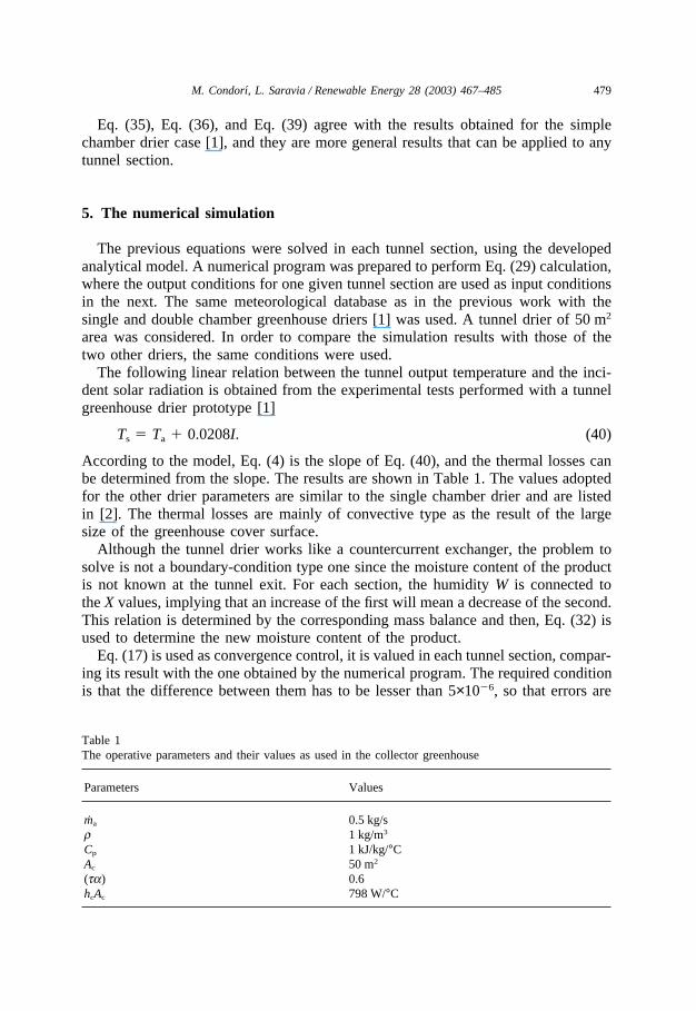
In Fig. 5, the simulated drying curve for the first section is compared with thecorresponding one to the first cart of the tunnel prototype. In general, the fit is good,being better for the first day. The larger dispersion occurs for the nightly records,since the soil-stored heat is delivered to the surrounding, increasing the evapor-ation rate.

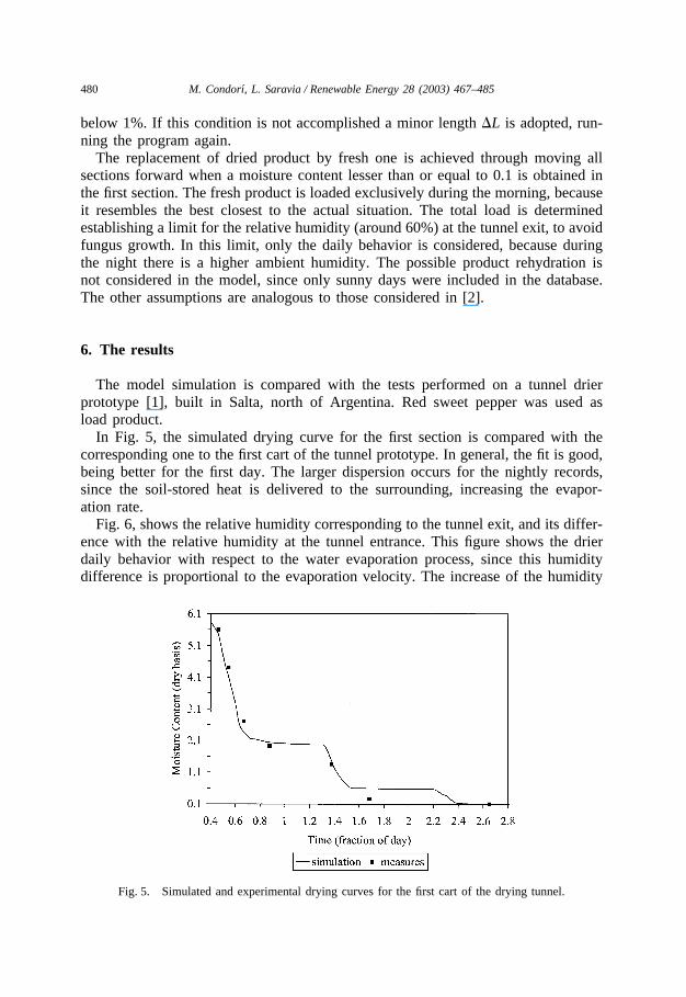
Fig. 6, shows the relative humidity corresponding to the tunnel exit, and its differ-ence with the relative humidity at the tunnel entrance. This figure shows the drierdaily behavior with respect to the water evaporation process, since this humiditydifference is proportional to the evaporation velocity. The increase of the humidity

Fig. 5. Simulated and experimental drying curves for the first cart of the drying tunnel.




Fig. 6. Above: relative humidity at the tunnel exit. Bottom: the relative humidity difference betweenthe exit and the entrance of the tunnel.

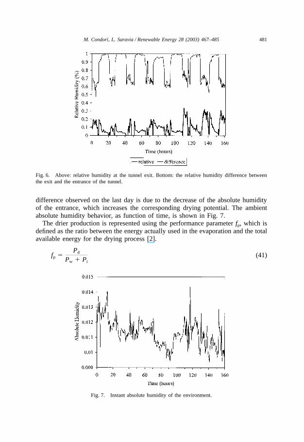
difference observed on the last day is due to the decrease of the absolute humidityof the entrance, which increases the corresponding drying potential. The ambientabsolute humidity behavior, as function of time, is shown in Fig. 7.

The drier production is represented using the performance parameter fp, which isdefined as the ratio between the energy actually used in the evaporation and the totalavailable energy for the drying process [2].

fp �Pd

Pw � Pi

(41)

Fig. 7. Instant absolute humidity of the environment.



Pd � qfmw

Pi � AsI

Pw � qfma[Ws(Ta)�Wa]

where Pd is the drier production expressed in energy units, Pi the drying potentialdue to the solar radiation, and Pw the drying potential due to the saturation deficitof the ambient air.

A non-dimensional variable Z defined as

Z �Pw

Pw � Pi

has all the meteorological information. The parameter fp is expressed as function ofZ and fp(Z) is defined as the drier characteristic function [2].

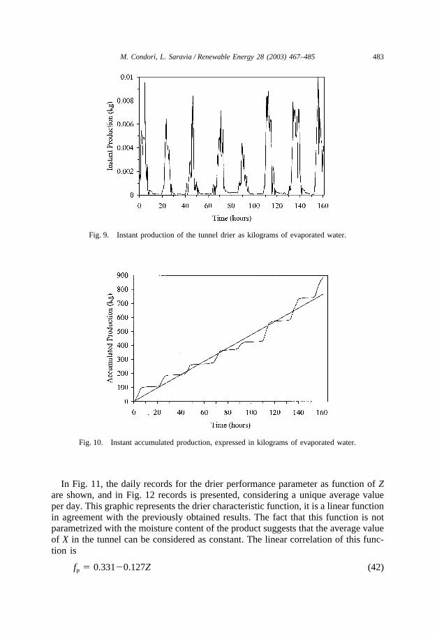
In Fig. 8, the drier performance parameter is shown as function of time. The sharppoints are due to the clouds presence. During the day, values rise upto 30% andthey go down to 20% during the night. Although, the nocturnal performance valuesseem high, the evaporation volume is small, as is shown in Fig. 9, where the instantdrier production is presented. During the nights, the only drying potential is thesaturation deficit, which decreases with the ambient temperature.

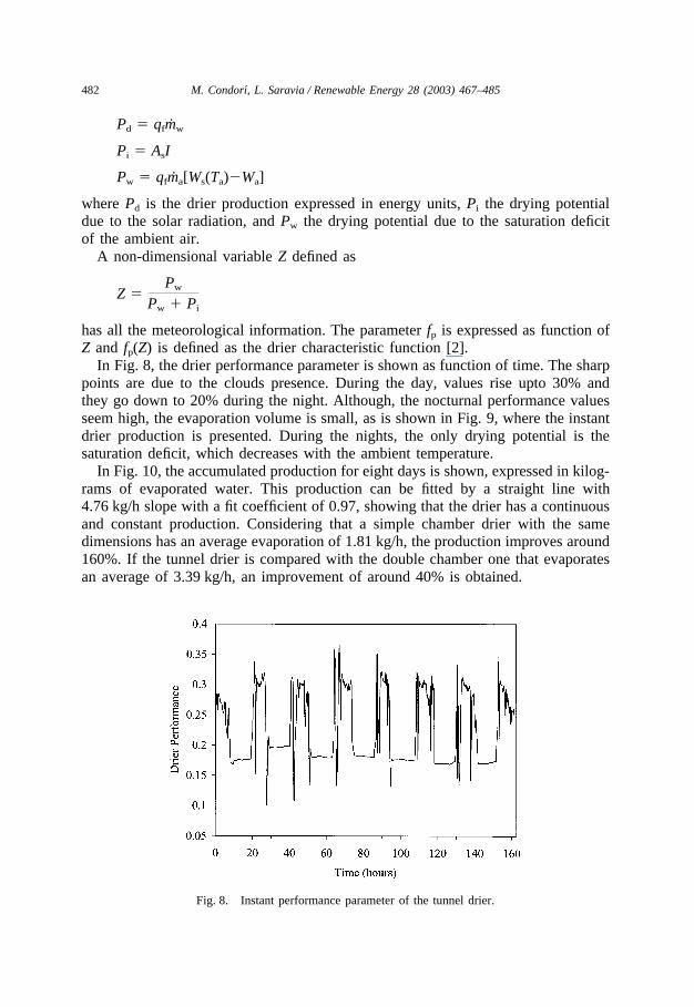
In Fig. 10, the accumulated production for eight days is shown, expressed in kilog-rams of evaporated water. This production can be fitted by a straight line with4.76 kg/h slope with a fit coefficient of 0.97, showing that the drier has a continuousand constant production. Considering that a simple chamber drier with the samedimensions has an average evaporation of 1.81 kg/h, the production improves around160%. If the tunnel drier is compared with the double chamber one that evaporatesan average of 3.39 kg/h, an improvement of around 40% is obtained.

Fig. 8. Instant performance parameter of the tunnel drier.



Fig. 9. Instant production of the tunnel drier as kilograms of evaporated water.

Fig. 10. Instant accumulated production, expressed in kilograms of evaporated water.

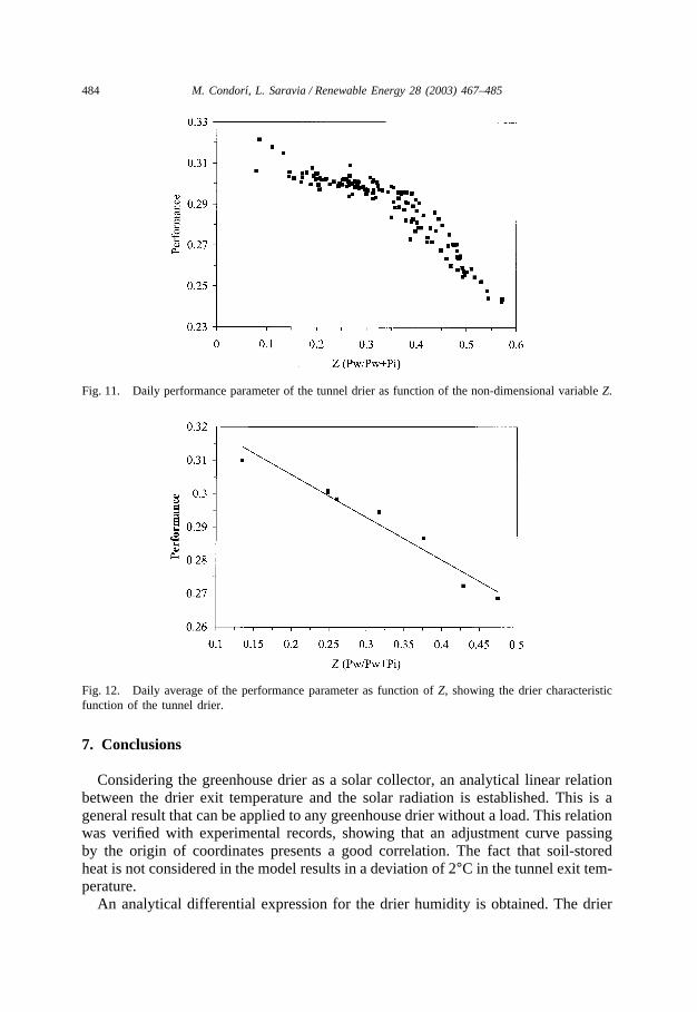
In Fig. 11, the daily records for the drier performance parameter as function of Zare shown, and in Fig. 12 records is presented, considering a unique average valueper day. This graphic represents the drier characteristic function, it is a linear functionin agreement with the previously obtained results. The fact that this function is notparametrized with the moisture content of the product suggests that the average valueof X in the tunnel can be considered as constant. The linear correlation of this func-tion is

fp � 0.331�0.127Z (42)


Fig. 11. Daily performance parameter of the tunnel drier as function of the non-dimensional variable Z.

Fig. 12. Daily average of the performance parameter as function of Z, showing the drier characteristicfunction of the tunnel drier.

7. Conclusions

Considering the greenhouse drier as a solar collector, an analytical linear relationbetween the drier exit temperature and the solar radiation is established. This is ageneral result that can be applied to any greenhouse drier without a load. This relationwas verified with experimental records, showing that an adjustment curve passingby the origin of coordinates presents a good correlation. The fact that soil-storedheat is not considered in the model results in a deviation of 2°C in the tunnel exit tem-perature.

An analytical differential expression for the drier humidity is obtained. The drier


accumulated production presents a linear relation with the drying time, showing thatthe drying potentials in the tunnel drier are properly used each day. Although theaverage performance is around 30%, it can be improved by optimizing the parametersK1 and K2, which are functions of the drying potential resistances. Particularly, thecover surface, through the global losses coefficient hcAc, has a strong incidence onthe drier thermal efficiency.

The performance function and the generalized drying curve concepts are applied,obtaining general results analogous to the single and double chamber drier cases.The tunnel drier characteristic function fp(Z), is a linear equation with negative slope.The origin ordinate represents the maximum possible performance obtained duringthe day, and the condition Z=1 determines the minimum possible performanceobtained during the night. The global drier production is constant, without appreci-able changes each day, and average moisture content of the product may be con-sidered constant for the tunnel.

A numerical simulation of the analytical model is run with the same database usedwith other driers to compare their behaviors. There is an improvement of around160% with respect to the single chamber drier, while the improvement is of about40% if compared with the double chamber drier.

Acknowledgements

This work was supported by the CONICET (Consejo Nacional de InvestigacionesCientıficas y Tecnicas).

References

[1] Condorı M, Echazu R, Saravia L. Solar drying of sweet pepper and garlic using a tunnel greenhousedrier. Renewable Energy 2000;22(4):447–60.

[2] Condorı M, Saravia L. The performance of forced convection greenhouse driers. Renewable Energy1998;13(4):453–69.

[3] Dufie JA, Beckman WA. Solar engineering of thermal processes, 2nd ed. New York: Wiley, 1991.[4] Edwards CH, Penney DE. Elementary differential equations with applications. New Jersey: Prentice-

Hall, 1985 (p. 101–30).





Documents

Analytical model for the performance of the tunnel-type greenhouse drier