arX

iv:c

ond-

mat

/031

0444

v1 [

cond

-mat

.dis

-nn]

19

Oct

200

3 Analysis of Norms Game in networked so ieties

Pawel Sobkowi z

19th O tober 2003

Abstra t

Norms, de�ned as generally a epted behaviour in so ieties without entral au-

thority (and thus distinguished from laws), are very powerful me hanism leading

to oherent behaviour of the so iety members. This paper examines, within a

simple numeri al simulation, the various e�e ts that may lead to norm forma-

tion and stability. The approa h has been �rst used by Axelrod, who proposed

two step model of norm and meta-norm enfor ement. We present here an ex-

tension and detailed analysis of the original work, as well as several new ideas

that may bear on the norm establishment me hanisms in so ieties. It turns out

that a relatively simple model for simulated norm enfor ement predi ts persis-

tent norm breaking even when it is asso iated with high punishment levels. The

key fa tors appear to be the ombination of the level of penalty for breaking

the norm and proximity of norm enfor ers. We also study a totally di�erent

me hanism of norm establishment, without meta-norms but using instead the

dire t bonus me hanism to norm-enfor ers.

1 De�nitions of the Norms Game variants

The original work of Axelrod [1℄, later reprinted and expanded, as Chapter 3

of [2℄ has des ribed a possible s enario for modelling norm formation, alled

the Norms Game (NG), and its higher level variant, the Meta Norms Game

(MNG). The games are based on extended Prisoner's Dilemma game, in luding

additional a tion by the rest of ommunity: punishment of a defe tor (NG),

and additional possibility of punishment of for failing to punish the defe tor

(MNG). The idea behind the model is to see if su h enfor ement may lead to

formation of stable ooperative so iety, and whether simple enfor ement has to

be augmented by meta-enfor ement, to a hieve stability of the system.

1.1 The lassi formulation of Norms Game.

The model presented by Axelrod is based on an N -person PD game. Within the

game, ea h player i has several "a tion opportunities" ea h turn, during whi h

he an either play safe, in whi h ase he gets no bene�t, or defe t in whi h

ase he gets a treasure of T > 0, while players j 6= i get extra harm H < 0.The willingness of an agent i to ommit a defe tion is alled boldness bi. For

obvious reasons, the only stable strategy in su h game is that of total defe tion

� ea h "safe player" is at distin t disadvantage with the defe tors.

1

The next step is the introdu tion of norm enfor ement a tivities (the

norm being understood as the neutral, safe behaviour).

If the player i does not defe t, other players do not take a tion. If, on

the other hand, i does break the norm, other players j may, with probability

vj (vengefulness), punish him for misbehaviour. In the original treatment,

the punishment value P was assumed greater than the treasure T . At the

same time, ea h punishing agent pays punishment osts E (enfor ement).

The punishment for defe tion onstitutes the proper Norms Game: so iety uses

a tive measures to enfor e the norms.

After ea h round of intera tions between agents, Axelrod used simple popu-

lation adjustment, giving higher population ratios to those players with higher

overall bene�ts. He has also used a small "mutation" rate to introdu e small

random shifts in strategies. Results of simulations were presented after 100 gen-

erations. In Axelrod's simulations two out of �ve runs ended up in boldness

b ≈ 1 and v ≈ 0, while other simulations ended with various levels of vengeful-

ness, with very small boldness. The pure norm enfor ing behaviour, depending

on the simulation history or initial onditions led to either almost fully defe ting

so iety or to one pa i�ed by vengefulness. Axelrod's argument was that pure

NG is too weak to ensure norm respe ting behaviour.

Introdu ing Meta Norms Game, as an extension of the previous model, Ax-

elrod proposed that if agent i defe ts and agent j does not punish i, then with

probability v′ any other agent k should punish j for failing to enfor e the norm!

The meta-punishment P ′and ost asso iated with it, E′

were assumed to be

equal to P and E.

More importantly, themeta-vengefulness v′ was assumed to be equal to v.This de ision was based on rather vague arguments. The link de�nitely simpli-

�ed al ulations, but, as noted by Axelrod himself, prohibited situations when

ertain agents would use di�erent values of v and v′ to their advantage. Resultsof simulations with v = v′ were uniform: in all ases the so iety onverged to

almost pure high vengefulness, low boldness, norm-observing one.

From his simulations Axelrod has on luded that, for pure Norms Game,

. . . at �rst, boldness levels fell dramati ally due to the vengefulness

in the population. Then, gradually, the amount of vengefulness also

fell be ause there was no dire t in entive to pay the enfor ement

ost of punishing the defe tion. On e vengefulness be ame rare, the

average level of boldness rose again, and then the norm ompletely

ollapsed. Moreover, the ollapse was a stable out ome.

In ontrast, the in lusion of meta-norm enfor ement had provided the agents

with a strong in entive to in rease their vengefulness and this to promote the

norm (de rease boldness). This was indeed on�rmed by the simulation results.

From one point of view this is obvious onsequen e of the model, in whi h

some hara teristi s are penalised (boldness in ase of NG, boldness and la k

of vengefulness in the ase of MNG). La k meta-vengefulness is not penalised

at all, just the opposite � it arries its own ost, and is thus disadvantageous

evolutionarily. This leads to minimization of the meta-vengefulness in the evo-

lution pro ess � unless, as in Axelrod's model, it is for ibly �xed, for example by

oupling it to vengefulness. By setting v = v′, P = P ′and E = E′

Axelrod has

not only simpli�ed the simulations, but also made a sort of self-poli ing model.

2

He has thus ex luded analysis treating meta-enfor ement and enfor ement as

independent yet intera ting phenomena.

Additionally, be ause in the original form, the Norms Game was played

with a very small number of agents (20) no s aling e�e ts were visible. One of

su h e�e ts is the umulation of penalties due to the model in whi h anyone is

apable of punishing everyone, and individual punishments add up. This results

in penalties easily "over oming" bene�ts of trespassing. Despite the mentioned

oversimpli� ations of the simulations themselves, the MNG model seems to be

interesting enough to use it as a basis for more detailed studies. A signi� ant

and open question remains whether the results would be hanged by larger and

longer simulations and by more �exible model.

1.2 Modi�ed form of Norms Game with single enfor ers

To extend the validity of the model and to he k if the assumptions made by

Axelrod ould be derived from more general prin iples we propose a modi�ed

form of MNG.

We assume that NT agents (NT ≫ 1) are onne ted via a network of on-

ne tions, ea h intera ting with a number of neighbors. In di�erent simulations

we have used four basi network topologies, typi al for biologi al or so ial net-

works. These types in luded: fully onne ted network, in whi h every agent

is onne ted with all others; random network, where agents are onne ted

by randomly distributed links; nearest neighbour network, where the links

are highly lustered and �nally the small world networks. The three latter

types of networks may be alled lo al, as the number of agents that a given

agent intera ts with (a tively or passively) is mu h smaller than the total num-

ber of agents. This limits the in�uen e and sets stage for possible indire t

in�uen es. General des ription of su h networks may be found in Albert and

Barabási [3℄, Dorogovtsev and Mendes [5℄, Dorogovtsev et al. [6℄, Dorogovtsev

and Mendes [4℄, Newman [7, 8℄, Newman and Park [9℄. All these networks are

hara terized by �lling ratio, whi h relates to the average number of links per

node (agent). The larger the �lling ratio, the more agents are dire tly onne ted.

In our simulations we have used ratios from 0.005 to 0.02 (whi h orresponds to

ir a 5 to 20 links per agent. The di�eren e between the various types of lo al

networks are in the way the agents are onne ted.

In random (RAND) networks the links are distributed randomly, thus we

have a meshed network of links, with agents di�ering in number of the neigh-

bours, and no general stru ture.

The nearest neighbor (NN) nets are formed by linking ertain number of

losest neighbors together. The easiest way to visualize su h network is to pla e

the agents on an imaginary ir le and onne ting ea h agent to n neighbors.

The number of onne tions per agent is onstant. Interesting property of NN

networks is that for small �lling fa tors, agents on the opposite points at the

ir le to ommuni ate must go through many intermediaries. For 2000 agents

and number of neighbors set at 10, the longest `distan e' is 100 `hops'. This

suggests in�uen e on the hanges in norm adheren e and enfor ement: any

hange of behavior of the agent i is seen immediately by his losest neighbors

(who an see him through dire t links) but only after onsiderable delay and

�ltering by members of so iety lo ated far from i.The Small World (SW) networks, introdu ed and popularized in re ent years,

3

reprodu e a urious fa t observed in many natural and human-produ ed net-

works, namely that the distan e between any two nodes of the network, mea-

sured in links needed to onne t them, is usually mu h smaller than that in

nearest neighbor or even random networks of the same �lling ratio. The name

of the network ategory omes exa tly from su h observation. One of the models

for SW networks is a simple reworking of the NN model: one takes a small (even

very small!) fra tion of the links from between nearest neighbors and applies

them instead between random agents. Keeping in mind the visualization of NN

networks as nodes along a ir le, this orresponds to adding onne tions that

riss- ross the ir le at random. Due to su h short uts, even if their number

is very small, the average distan e between any two nodes drops dramati ally.

Thus we have a network that for ea h agent, lo ally is very similar to NN model

(as most of the neighbors are, in fa t, the same), but globally the ommuni ation

through the network is mu h faster.

Within our MNG s enario ea h agent has a hoi e between a ting in a or-

dan e with a norm, in whi h ase he gets no extra bonus, or breaking the norm

(trespassing), in whi h ase he gets extra bonus (treasure) T . If the agent imisbehaves, every agent in the population is harmed by this a tion. We an

imagine this orresponds, for example, to the agent stealing some ` ommunal

property'. The treasure T is the bene�t to the trespasser, but the harm H to

the ommunity may be greater than T . It is then assumed that the harm H is

divided evenly among population, ea h agent `losing' H/NT .

Let's denote the probability of misbehavior (boldness) of agent i by bi. The

payo� X(i) of agent i is (without any punishments) given by

X(i) = biT − NT 〈b〉T H/NT = biT − H〈b〉T (1)

where 〈b〉T denotes average of bi over the total population. With H > T the

overall average payo� be omes negative 〈b〉T (T −H) and is disadvantageous to

the ommunity, but as any agent with boldness higher than the average gets

more bene�t than the rest, su h behaviour gives evolutionary advantage, and

thus multiplies. Natural end of su h a pro ess is a free-for-all, bi = 1 so iety.

As in Axelrod's work we propose that to urb boldness, so iety enfor es the

norm through penalization of trespassing. Our model di�ers slightly in the way

the pro ess of dete tion and punishment is en oded.

Ea h agent wat hes his neighbours for a ts of misbehavior and is may be

willing to punish for su h a ts. For an agent j with vengefulness vj the prob-

ability of dete tion that another agent i has broken the norm is just vj . The

wat hfulness and vengefulness result in enfor ement e�ort E, the overall ost of

being vigilant to an agent j being vjE. The �rst agent to noti e that someone

has broken the norm punishes the transgressor with a punishment of P . Thus

only one punishment a t take pla e and there is no umulation e�e ts, but the

value of P may be set freely. To al ulate the expe ted penalty value we start

with the probability of no-one dete ting the misbehaviour of i is

∏

(j 6=i)

(1 − vj), (2)

where the produ t is taken over all agents j with links to i, that is over the

4

neighbours of i. As a result the penalty for agent i would be given by

πP (i) =

1 −∏

(j 6=i)

(1 − vj)

biP, (3)

that is proportional to probability is at least one agent dete ting the a t of

breaking the norm times probability of su h a t times the penalty value. With-

out meta-norms the payo� for player i is thus

biT − H〈b〉T − viE −

1 −∏

(j 6=i)

(1 − vj)

biP (4)

So far the di�eren e between the modi�ed model and Axelrod's one was in

the fa t that the punishment takes pla e only on e. The real hange omes in

the way the meta-norm is introdu ed. In the original model every failure to

punish a norm breaker was meta-punished. Here, we have only one punishing

agent (the �rst one to dete t the trespasser). The problem is how should the

meta-enfor er de ide whether non-punishment by ertain agent was intentional

(due to la k of vengefulness or it's small value) or just a result of oming in

se ond, after the enfor ement has already taken pla e? One way is to set the

probability of meta-punishment as being proportional to the la k of vengefulness

of the observed agent:

XMP (j, i) = v′j(1 − vi), (5)

with v′j being the meta-vengefulness of the observing agent j and 1 − vi being

the la k of vengefulness of the observed agent i. Thus the expe ted value of

meta-punishment for an agent i is

πMP (i) =

1 −∏

(j 6=i)

(1 − XMP (j, i))

P ′(6)

As our simulations were on eived as extension of the work of Axelrod, we

have used similar onvention of allowing dis retized values of bi, vi and v′i (from0 to 1 with steps of 0.1). To see if su h dis retization does not produ e any

arti� ial e�e ts we have also performed al ulations in whi h boldness, venge-

fulness and meta-vengefulness were allowed to take arbitrary values between 0

and 1. To our slight surprise the results did not di�er signi� antly. The spe i�

results presented in this paper refer to the dis rete model.

1.2.1 Results of NG and MNG for large fully onne ted networks

Lets turn now to the NG and MNG played in relatively large, fully onne ted

networks. Here every agent intera ts with all agents as in the ase of the small

model of Axelrod, and the evolution seems rather simple. The most important

fa t here is that even a single enfor er or meta-enfor er (say an a idental mu-

tant) would be able to in�uen e the payo�s of all agents, and dire t the ourse

of evolution of population.

Lets onsider �rst the situation where there is no meta-norm enfor ement at

all (P ′ = 0). If one starts from a random population in all simulations the �nal

5

average value of vengefulness was v = 0. This is due to additional osts borne bythe enfor ers, and the pressure to minimize this ost. However, as initially there

were some norm enfor ers (and remember that in a fully onne ted network just

one mutant would su� e to enfor e the norm on the whole population!) the

enfor ement put a lear divide between two basi situations. When the treasure

T is greater than P it pays to be bold, and b → 1. On the ontrary, for T < Pwe have b → 0. This orresponds to ommon sense observation that the norm

would be obeyed if the penalty for breaking it would be sure (whi h is made

probable by large number of observers) and greater than the bene�ts.

When the meta-norm enfor ement is present the situation shifts to meta-

level. In all simulations the �nal average value of meta-vengefulness goes to zero

(v′ → 0) � due to the same arguments as vengefulness dropped in previously

des ribed simulation. However, as already noted, in a fully onne ted network

even a single meta-enfor er is able to meta-punish everyone in so iety! Thus,

although nominally the number of these meta-enfor ers goes is zero in the stable

situation, their initial in�uen e and o asional mutant presen e are su� ient to

distinguish the situation from the previously des ribed ase of P ′ = 0.The results of simulations di�er in small details (su h as the number of

iterations it takes to a hieve stability) but in prin iple are governed by two

simple rules.

• The boldness is de ided by relation of T vs. P , as des ribed above

• The vengefulness is de ided by relation of the ost of vengefulness E and

the meta-punishment P ′

Again, the above results are very mu h ommon sense. De oupling v from

v′ results in v′ → 0 for MNG, whi h ontrasts the assumed v = v′ in Axelrod

approa h. Large size of the population leads to elimination of `unde ided' runs

� all simulations ended with uniform populations.

1.2.2 Lo al networks

In ontrast to the fully onne ted ase, the lo al networks present mu h more

interesting norms dependen e on the payo� parameters.

As in the original formulation of MNG, in addition to a breeding me ha-

nism, in whi h ertain per entage of agents with the best payo�s were allowed

to breed (at the ost of the worst faring agents), we have used additional mu-

tation pro ess. This was simulated as allowing ertain fra tion of agents (given

by mutation ratio) to hange their hara teristi bi, vi and v′i values between

intera tions. Although the number of mutants per iteration was usually kept

very small in relation with the population size (e.g. 2 mutants out of 2000

per iteration), its e�e ts were quite important. Without mutation populations

sometimes froze in a given on�guration, `far' from results obtained with even

minimal mutation rates.

Another e�e t we set out to investigate was the dependen e of the behaviour

on the starting onditions. Two general types of starting onditions were used:

in the �rst the initial populations had randomly distributed values of bi, vi and

v′i. In the se ond, we have started from pure so iety of, for example, bi = 0,vi = 1 and v′i = 0, or bi = 1, vi = 1 and v′i = 0 � to observe if su h pure so ieties

were evolutionary stable with respe t to small mutation rates. It turned out that

6

regardless of the starting ondition, if the mutation was present, the �nal state

was very similar.

We present general results of simulation runs through a few examples, and

dis uss the role of the starting onditions. The simulations were run for 2000

agents using �xed values of P = 20, P ′ = 3, E′ = 1, H = 12, with top 1% of

the population being allowed to reprodu e ea h iteration (at the expense of the

bottom 1%). Other parameters (T , E) were used to ontrol the simulations and

the dependen e on them is presented and dis ussed below.

1.2.3 Similarities and di�eren es between random, NN and SW net-

works

In our simulations we ompare results for all three types of lo al networks.

Despite the fa t that the three types of lo ally onne ted networks have many

di�erent properties (see, for example [3, 5, 6, 4℄) the results of our simulations

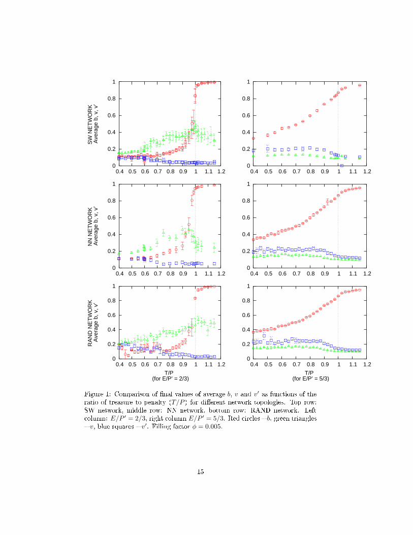
for random, small world and nearest neighbour networks are strikingly similar

(see Figure 1). It turns out that the key fa tor is the ommon hara teristi of all

models, given in the �rst approximation by the average number of neighbours.

The number of neighbors is related network �lling fa tor φ, de�ned as ratio of

the a tual links in the network to the total possible number of links:

φ =NLINKS

NT (NT − 1)/2. (7)

For regular networks, su h as NN network, the number of neighbors is the

same for all agents, NN = NLINKS = φNTOT /2. For small world networks,

onstru ted as in this work, the NN de�ned above is a very lose measure of

the number of neighbors, with very few ex eptions. For random networks, the

dispersion in number of links per agent is greater, but still NN gives the average

value.

The di�eren es between lo al network topologies for the same �lling fa tor

values are relatively small. Thus the use of the word `lo al' is justi�ed: behaviour

of an agent is then determined by his immediate surrounding, mainly by the

number of agents who observe it and vi e-versa, the number of agents it observes.

The two verti al olumns of plots in Figure 1 orrespond to two ases of E/P ′

ratio. The left olumn has E/P ′ = 2/3 < 1, whi h in the ase of fully onne ted

network would orrespond to large vengefulness v � so, to strong pressure to

de rease b. The right olumn has E/P ′ = 5/3, with meta-penalty smaller

than the ost of being vigilant there is little in entive to be a norm enfor er.

Indeed, the results of simulations for the two ases are strikingly di�erent. For

E/P ′ < 1 v is relatively large and b resembles the step-like fun tion found in

fully onne ted network. v′ remains relatively small. On the other hand, for

E/P ′ > 1 v is smaller, v′ larger, and the step like hara ter of b is repla ed

by gradual growth. This orresponds to the presen e of trespassers who, in

lo al environments, �nd that lo ally the e�e tive punishment is smaller than

the treasure value. Thus even at T/P mu h smaller than 1 we have relatively

high average b.

1.2.4 Dis ussion of the dependen e on the �lling fa tor

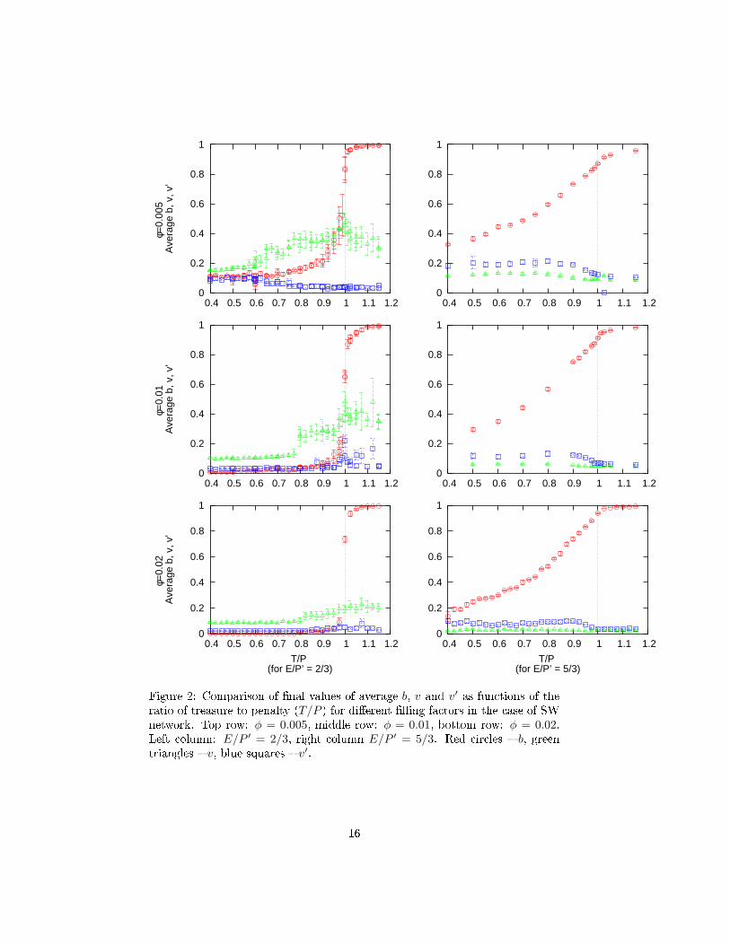
Figure 2 presents another set of omparisons of the average �nal b, v and v′

values, this time for a single type of the network topology (Small World) but

7

di�ering by the �lling fa tor φ. The top row orresponds to φ = 0.005, middle

row to φ = 0.01, bottom row to φ = 0.02. Corresponding average number of

neighbours hanges from 5 to 20. For the ase of E/P ′ = 5/3 (right olumn)

the di�eren e is visible mostly in lowering values of v and v′ below T/P = 1,and in more pronoun ed kink in b at T/P = 1 with in reasing φ.

For E/P ′ = 2/3 one an observe two e�e ts:

• a shift of the step-like in rease of b as fun tion of T/P to values lower

than 1;

• an in rease in vengefulness v in the region of T far below P for E = 2,where simple explanations suggest no dependen e of v over T .

The �rst e�e t an �nd a qualitative explanation through analogy with sim-

pli�ed, small size fully onne ted model. Then the �nite size of neighbourhood

hanges the ondition for the misbehaviour to be advantageous from T > P to:

Ti > P

1 −∏

j 6=i

(1 − vj)

≃ P(

1 − (1 − v)NN

)

(8)

with v being the average vengefulness. The expression P(

1 − (1 − v)NN

)

may

be dubbed the e�e tive deterrent, as it weights the penalty with probability of

being punished. For large number of neighbors NN the term (1 − v)NNgoes to

zero, and we re over the T > P ondition. For small NN the di�eren e is visible

as the shift of the step in b(T ) fun tion.

1.3 Simulations with group enfor ement

The previous se tions have dis ussed the extreme opposite to Axelrod's assump-

tion of additive punishment � only a single agent was exe uting the punishment,

and it was assumed that this single agent had enough power to e�e t the pun-

ishment on anyone it had links with. Within this model a single enfor er or

meta-enfor er ould `poli e' the whole neighbourhood.

It is interesting to see if the results obtained in previous simulations would

be hanged when one would require some greater number of agents, a ting in

unison, to e�e t a punishment or meta-punishment. Su h situation of `group

a tion', or oalition forming against a trespasser seems more similar to `real life'.

Lets assume that the punishment would take pla e if at least kP neighbors

of trespassing agent i would be willing to enfor e the norm. Similarly, meta-

punishment would require kMP neighbors to a t together. In our al ulations

we would limit ourselves to low values of kP and kMP of 2 and 3.

To obtain the expressions for group punishment model one starts with Φm(i)and Ψm(i) de�ned as: probability that exa tly m neighbors if agent i would be

willing to enfor e the norm (or meta-norm) on i. We have:

Φ0(i) =∏

j 6=i

(1 − vj) (9)

Φ1(i) =∑

k 6=i

∏

j 6=i,k

vk(1 − vj) (10)

Φ2(i) =∑

k 6=i

∑

l>k,l 6=i

vkvl

∏

j 6=i,k,l

(1 − vj) (11)

8

Φ3(i) =∑

k 6=i

∑

l>k,l 6=i

∑

m>l,m 6=i

vkvlvm

∏

j 6=i,k,l,m

(1 − vj) (12)

Ψ0(i) =∏

j 6=i

(

1 − v′j(1 − vi))

(13)

Ψ1(i) =∑

k 6=i

v′k(1 − vi)∏

j 6=i,k

(

1 − v′j(1 − vi))

(14)

Ψ2(i) =∑

k 6=i

∑

l>k,l 6=i

v′kv′l(1 − vi)2∏

j 6=i,k,l

(

1 − v′j(1 − vi))

(15)

Ψ3(i) =∑

k 6=i

∑

l>k,l 6=i

∑

m>l,m 6=i

v′kv′lv′m(1 − vi)

3∏

j 6=i,k,l,m

(

1 − v′j(1 − vi))

(16)

Thus, requiring that more than kP agents (who are neighbors) de ide group

together and punish transgressor i (or respe tively kMP agents group to meta-

punish i) we have the expression for punishment (meta-punishment)

πkP

P (i) =

(

1 −

kP∑

k=0

Φk(i)

)

biP (17)

πkP

MP (i) =

(

1 −

kMP∑

k=0

Ψk(i)

)

P ′(18)

Obviously, for kP = 0 and kMP = 0 (whi h orresponds to just one agent being

able to e�e t punishment) the above expressions redu e to Equations 3, 6.

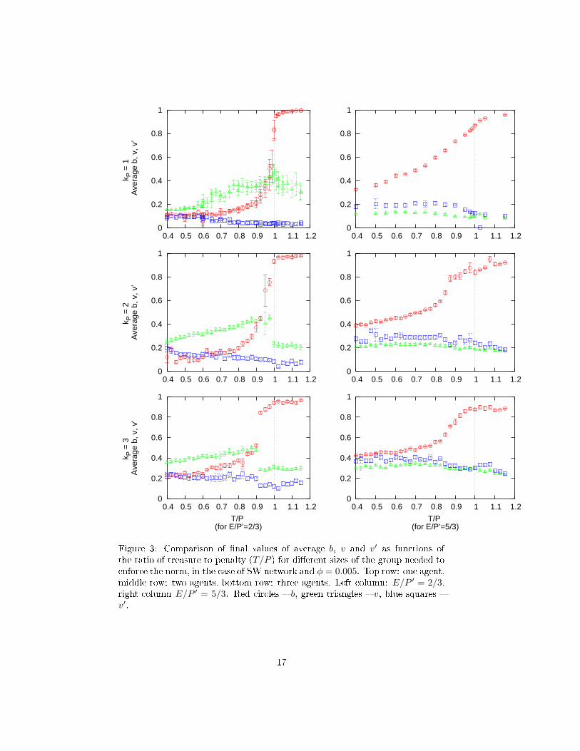
Figure 3 ompares results for SW network at low �lling fa tor φ = 0.005,where the problems related to the need to �nd enough enfor ers for the group

a tion should be most visible, for three values of kP = 1, 2, 3 (top, middle and

bottom row respe tively). The shift of high b regime to regions of T/P < 1 is

even more pronoun ed than in Figure 2, the reason being lear: it is in reasingly

more di� ult to �nd two and three agents a ting in unison in neighborhoods

of average size of 5. However, there is no radi al hange in behaviour of the

system as the whole.

2 To enfor e or to break the norm?

In Axelrod's study as well as in the results presented above, boldness and venge-

fulness were treated as separate hara teristi s of an agent. Details of our sim-

ulations show that in most ases the best payo�s are a hieved by agents who

at the same time take advantage from breaking the norm and a tively pursue

enfor ement on other trespassers, that is agents with simultaneously high b andv. while perfe tly a eptable from mathemati al point of view, this is somewhat

against psy hologi al expe tations: one an either be a poli eman or a thief. We

dub this ase the ex lusive model.

To see if su h ontradi tion of hoi es has in�uen e on the simulated so ieties

we have performed series of runs in whi h bi and vi were oupled through vi =1 − bi, that is, the more the agent a ted as trespasser (higher bi) the smaller

was his vengefulness. This simple relation does not re�e t the omplexity of the

issue of the ex lusivity of hoi es, but allows an insight into possible out omes.

9

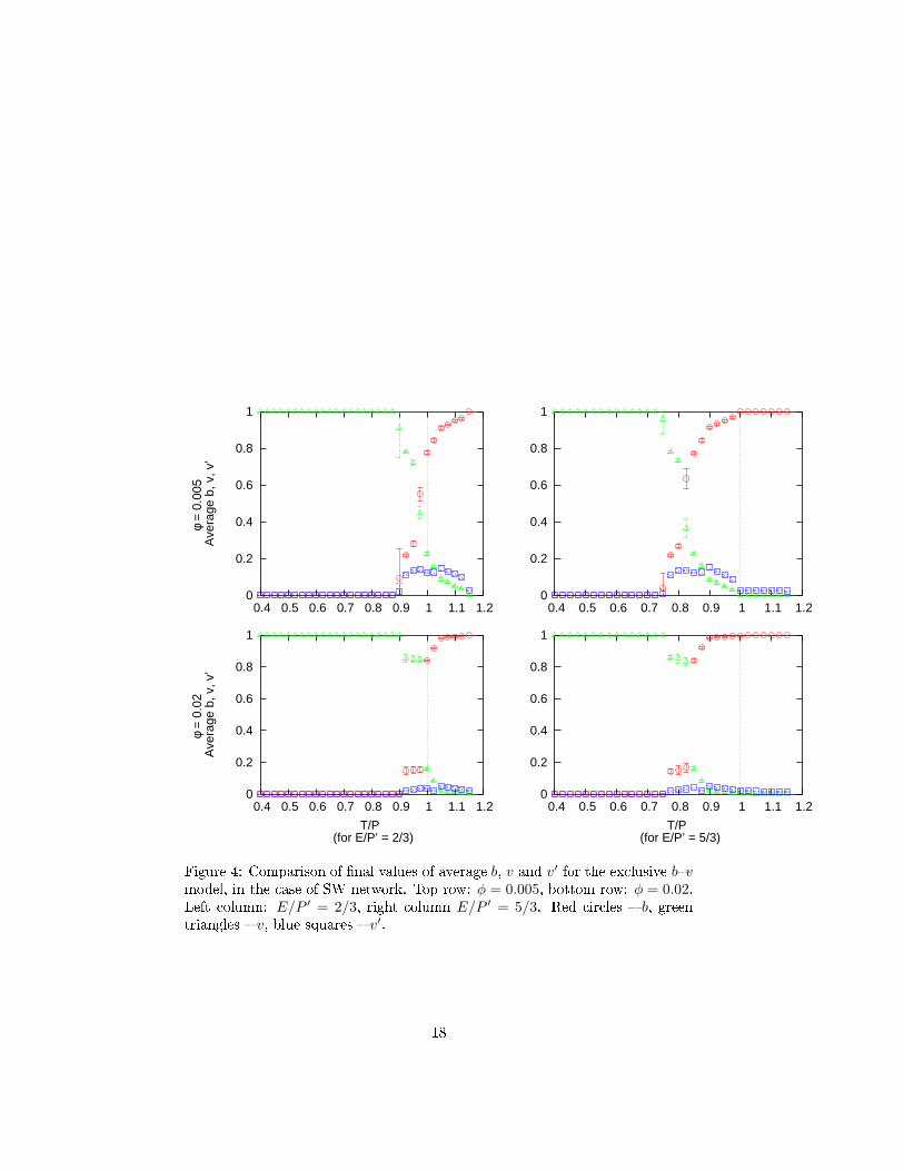
The simulations returned quite interesting results, as presented in Figure 4

for SW network at two �lling fa tors (φ = 0.005 and φ = 0.02), with single

agent enfor ement. For small T/P stable result was b = 0 and v = 1. For

large T/P the opposite result was true. The width of the transition region

depends on the �lling fa tor, for larger number of neighbors the region was

mu h narrower. The hange in the value of the of E resulted in almost dire t

shift of the of the step-like in rease of b as fun tion of T toward lower T . Theonset of the norm-breaking behaviour was given by simple relation T0 = P −E.

This orresponds to ondition when the bene�t of norm breaking (T ) ex eedsthe optimum bene�ts of the enfor ers (P − E).

The ex lusive b�v model ould be enhan ed in a way that instead of using

relation b = 1 − v (whi h allows an agent to a t `a bit as a poli eman and a

bit as a thief') one would use more ompli ated rule. This may be subje t of

separate investigation.

3 Norm enfor ement through bounty hunting

Within Axelrod's model vengefulness and meta-vengefulness were dire tly ou-

pled. In our extension of the approa h des ribed above we have de oupled them,

and studied in�uen e of the meta-enfor ement of the norm persisten e. There

is, however another interesting possibility, whi h is based on simpli�ed observa-

tions of `real life' situations, where norm enfor ement, although in itself ostly

(through onstant wat hfulness ost E), may be positively reinfor ed, without

resorting to meta-norms.

The me hanism is quite simple. Suppose the trespasser is aught. Then the

agent or agents who have aught him would get a bounty B. The bounty may

be set arbitrarily, but in out simulations we use the following s enario. The

e�e tive penalty πkP

P (j) may be treated as a �ne imposed on the trespasser j.Part of it a ounts for general osts, but the rest, des ribed through fra tion

f , is divided among all agents that have parti ipated in the a t of enfor ement

on the trespasser (or, to formulate it within the model used here, among all

agents that might have parti ipated in the a t of enfor ement). This allows for a

strategy using bounty hunting as means of in reasing the payo� of an agent,

and thus in reases v, whi h might help in keeping b down.

Suppose we want to establish the payo� for agent i for at hing a trespassingagent j. The whole bounty fπkP

P (j) has to be divided among all agents k that

are neighbors of j, in a way that relates to their ability and willingness to enfor ethe norm. We introdu e a simple (though arbitrary) formula that preserves the

relation of the individual bounties B(i, j) to the vengefulness e�ort. First we

introdu e the summed vengefulness around agent j:

vSj =

(neighbors of j)∑

k

vk, (19)

where summation goes over all neighbors of j. Using this it is easy to divide

the bounty: the bounty for agent i for at hing trespasser j (who's willingness

to break the norm is given by boldness bj) is

B(i, j) = fπkP

P (j)vi/vSj . (20)

10

Thus the total bounty payo� for agent i is given by:

B(i) =∑

j

B(i, j) = fPvi

(neighbors of i)∑

j

bj

∑kP

n=0 (1 − Φn(j))∑(neighbors of j)

k vk

(21)

For large number of enfor ers with high vengefulness, the bounty would be

divided among many agents, and thus relatively small. But suppose there is

just a few enfor ers � they would get signi� ant advantage for at hing the

trespassers. The model has, in pla e of P ′and E′

only a single parameter f ,des ribing how mu h of the penalty P is divided among the vengeful agents.

The new formula for payo�s repla es the meta-enfor ement terms with the

bounty term. The simulation spa e is now simpler (two-dimensional, with vari-

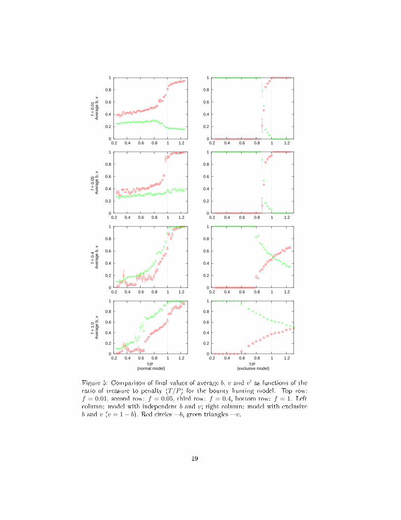
ables b and v). Example of simulation results is presented in Figure 5. Left

olumn shows average b and v values as fun tions of T/P , right olumn shows

results for the ex lusive model dis ussed in previous se tion.

Rows orrespond to in reasing fra tions of the penalty divided as bounty

among enfor ers, from f = 0.01, through f = 0.05 and f = 0.4 to f = 1. It isworth noting that as ea h agent has on average 5 neighbors, these fra tions allow,

in prin iple to get quite signi� ant payo� from bounty. With our simulation we

have set the enfor ement ost at E = 2 and penalty P = 20. Thus the bountyfrom 5 trespassers at f = 0.05 might rea h 5, over oming the ost of being

vengeful.

As a result in the model with independent b and v only for very low f we

observe behaviour resembling the one found in MNG simulations. For larger fboth b and v in rease simultaneously, in a smooth way. These results form the

best illustration of the statement that it pays best to be a thief and poli emen

at the same time.

For the ex lusive ase the growth of b is quite similar, with v mirroring it

a ording to ondition v = 1 − b. The onset of the in rease of b as fun tion of

T/P takes pla e at almost the same values for both the normal and ex lusive

models

4 Con lusions

The on lusions of our models and simulations may be summarized as follows:

• de oupling norm enfor ement and meta-norm enfor ement (v and v′), setas equal in the original model of Axelrod, has shown that the quantities

evolve in very di�erent ways, thus the original assumption was probably

introdu ing arti� ial e�e ts into results presented in [1, 2℄;

• for large (more than 20 agents), fully onne ted so ieties, boldness and

vengefulness followed simple rules, dire tly relating them to net payo�s

for trespassers and enfor ers (T > P , P ′ > E);

• lo ally networked so ieties show ompli ated interplay of various param-

eters, with the leading role of the T/P and E/P ′ratios and strong de-

penden e on the �lling fa tor (number of neighbours). No dis ernible

di�eren es were observed for di�erent network topologies;

11

• in all ases we have observed lo al `po kets' of norm breakers (high bagents) well below the limit of T/P = 1;

• a variant of the model, aimed at repli ating the di hotomy of hoi e norm

breaking/norm enfor ement, in the simplest form of setting v = 1 − bleads to a smoothed step like behaviour of b, with the position of the step

de ided by T vs P − E, and its width by the number of neighbours;

• a new model, Bounty Norms Game (BNG), alternative to Meta Norms

Game, based on the division of part of the penalty among norm enfor ers

has been presented. Despite totally di�erent nature of the pro ess govern-

ing the evolutionary bene�ts of enfor ement the results resemble in general

way results from MNG simulations. Simpli ity and `real life' ba kground

of BNG make it a good andidate for at least some of the norm enfor e-

ment studies.

12

Referen es

[1℄ Axelrod, R. (1986). An evolutionary approa h to norms. Ameri an Politi al

S ien e Review 80, 1095�1111.

[2℄ Axelrod, R. (1997). The Complexity of Cooperation. Prin eton University

Press.

[3℄ Albert, R. and A. L. Barabási (2002). Statisti al me hani s of omplex

networks. Review of Modern Physi s 74, 67�97.

[4℄ Dorogovtsev, S. and J. Mendes (2002a). A elerated growth of networks.

In S. Bornholdt and H. S huster (Eds.), Handbook of Graphs and Networks:

From the Genome to the Internet, pp. 320�343. Wiley-VCH.

[5℄ Dorogovtsev, S. and J. Mendes (2002b). Evolution of networks. Advan es

in Physi s 51, 1079�1087.

[6℄ Dorogovtsev, S., J. Mendes, and A. Samukhin (2002). Prin iples of statisti al

me hani s of random networks. Nu l. Phys. B 666, 396�416.

[7℄ Newman, M. E. J. (2000). Models of the small world. J. Stat. Phys. 101,

819�841.

[8℄ Newman, M. E. J. (2003). Random graphs as models of networks. In S. Born-

holdt and H. G. S huster (Eds.), Handbook of Graphs and Networks. Wiley-

VCH.

[9℄ Newman, M. J. and J. Park (2003). Why so ial networks are di�erent from

other types of networks. submitted to Phys. Rev. E .

13

5 Figures

14

0

0.2

0.4

0.6

0.8

1

0.4 0.5 0.6 0.7 0.8 0.9 1 1.1 1.2

SW

NE

TW

OR

K

Ave

rage

b, v

, v’

0

0.2

0.4

0.6

0.8

1

0.4 0.5 0.6 0.7 0.8 0.9 1 1.1 1.2

0

0.2

0.4

0.6

0.8

1

0.4 0.5 0.6 0.7 0.8 0.9 1 1.1 1.2

NN

NE

TW

OR

K

Ave

rage

b, v

, v’

0

0.2

0.4

0.6

0.8

1

0.4 0.5 0.6 0.7 0.8 0.9 1 1.1 1.2

0

0.2

0.4

0.6

0.8

1

0.4 0.5 0.6 0.7 0.8 0.9 1 1.1 1.2

RA

ND

NE

TW

OR

K

Ave

rage

b, v

, v’

T/P (for E/P’ = 2/3)

0

0.2

0.4

0.6

0.8

1

0.4 0.5 0.6 0.7 0.8 0.9 1 1.1 1.2

T/P (for E/P’ = 5/3)

Figure 1: Comparison of �nal values of average b, v and v′ as fun tions of theratio of treasure to penalty (T/P ) for di�erent network topologies. Top row:

SW network, middle row: NN network, bottom row: RAND network. Left

olumn: E/P ′ = 2/3, right olumn E/P ′ = 5/3. Red ir les � b, green triangles

� v, blue squares � v′. Filling fa tor φ = 0.005.

15

0

0.2

0.4

0.6

0.8

1

0.4 0.5 0.6 0.7 0.8 0.9 1 1.1 1.2

φ=0.

005

Ave

rage

b, v

, v’

0

0.2

0.4

0.6

0.8

1

0.4 0.5 0.6 0.7 0.8 0.9 1 1.1 1.2

0

0.2

0.4

0.6

0.8

1

0.4 0.5 0.6 0.7 0.8 0.9 1 1.1 1.2

φ=0.

01

Ave

rage

b, v

, v’

0

0.2

0.4

0.6

0.8

1

0.4 0.5 0.6 0.7 0.8 0.9 1 1.1 1.2

0

0.2

0.4

0.6

0.8

1

0.4 0.5 0.6 0.7 0.8 0.9 1 1.1 1.2

φ=0.

02

Ave

rage

b, v

, v’

T/P (for E/P’ = 2/3)

0

0.2

0.4

0.6

0.8

1

0.4 0.5 0.6 0.7 0.8 0.9 1 1.1 1.2

T/P (for E/P’ = 5/3)

Figure 2: Comparison of �nal values of average b, v and v′ as fun tions of theratio of treasure to penalty (T/P ) for di�erent �lling fa tors in the ase of SW

network. Top row: φ = 0.005, middle row: φ = 0.01, bottom row: φ = 0.02.Left olumn: E/P ′ = 2/3, right olumn E/P ′ = 5/3. Red ir les � b, greentriangles � v, blue squares � v′.

16

0

0.2

0.4

0.6

0.8

1

0.4 0.5 0.6 0.7 0.8 0.9 1 1.1 1.2

k P =

1

Ave

rage

b, v

, v’

0

0.2

0.4

0.6

0.8

1

0.4 0.5 0.6 0.7 0.8 0.9 1 1.1 1.2

0

0.2

0.4

0.6

0.8

1

0.4 0.5 0.6 0.7 0.8 0.9 1 1.1 1.2

k P =

2

Ave

rage

b, v

, v’

0

0.2

0.4

0.6

0.8

1

0.4 0.5 0.6 0.7 0.8 0.9 1 1.1 1.2

0

0.2

0.4

0.6

0.8

1

0.4 0.5 0.6 0.7 0.8 0.9 1 1.1 1.2

k P =

3

Ave

rage

b, v

, v’

T/P (for E/P’=2/3)

0

0.2

0.4

0.6

0.8

1

0.4 0.5 0.6 0.7 0.8 0.9 1 1.1 1.2

T/P (for E/P’=5/3)

Figure 3: Comparison of �nal values of average b, v and v′ as fun tions of

the ratio of treasure to penalty (T/P ) for di�erent sizes of the group needed to

enfor e the norm, in the ase of SW network and φ = 0.005. Top row: one agent,middle row: two agents, bottom row: three agents. Left olumn: E/P ′ = 2/3,right olumn E/P ′ = 5/3. Red ir les � b, green triangles � v, blue squares �

v′.

17

0

0.2

0.4

0.6

0.8

1

0.4 0.5 0.6 0.7 0.8 0.9 1 1.1 1.2

φ =

0.0

05

Ave

rage

b, v

, v’

0

0.2

0.4

0.6

0.8

1

0.4 0.5 0.6 0.7 0.8 0.9 1 1.1 1.2

0

0.2

0.4

0.6

0.8

1

0.4 0.5 0.6 0.7 0.8 0.9 1 1.1 1.2

φ =

0.0

2 A

vera

ge b

, v, v

’

T/P (for E/P’ = 2/3)

0

0.2

0.4

0.6

0.8

1

0.4 0.5 0.6 0.7 0.8 0.9 1 1.1 1.2

T/P (for E/P’ = 5/3)

Figure 4: Comparison of �nal values of average b, v and v′ for the ex lusive b�vmodel, in the ase of SW network. Top row: φ = 0.005, bottom row: φ = 0.02.Left olumn: E/P ′ = 2/3, right olumn E/P ′ = 5/3. Red ir les � b, greentriangles � v, blue squares � v′.

18

0

0.2

0.4

0.6

0.8

1

0.2 0.4 0.6 0.8 1 1.2

f = 0

.01

Ave

rage

b, v

0

0.2

0.4

0.6

0.8

1

0.2 0.4 0.6 0.8 1 1.2

f = 0

.05

Ave

rage

b, v

0

0.2

0.4

0.6

0.8

1

0.2 0.4 0.6 0.8 1 1.2

f = 0

.4

Ave

rage

b, v

0

0.2

0.4

0.6

0.8

1

0.2 0.4 0.6 0.8 1 1.2

f = 1

.0

Ave

rage

b, v

T/P (normal model)

0

0.2

0.4

0.6

0.8

1

0.2 0.4 0.6 0.8 1 1.2

0

0.2

0.4

0.6

0.8

1

0.2 0.4 0.6 0.8 1 1.2

0

0.2

0.4

0.6

0.8

1

0.2 0.4 0.6 0.8 1 1.2

0

0.2

0.4

0.6

0.8

1

0.2 0.4 0.6 0.8 1 1.2

T/P (exclusive model)

Figure 5: Comparison of �nal values of average b, v and v′ as fun tions of theratio of treasure to penalty (T/P ) for the bounty hunting model. Top row:

f = 0.01, se ond row: f = 0.05, third row: f = 0.4, bottom row: f = 1. Left

olumn: model with independent b and v; right olumn: model with ex lusive

b and v (v = 1 − b). Red ir les � b, green triangles � v.

19