1

Analysis of LT Codes with Unequal Recovery

Time

Jesper H. Sørensen∗, Petar Popovski∗, Jan Østergaard∗, ∗Aalborg University,

Department of Electronic Systems, E-mail:jhs, petarp, jo@es.aau.dk

Abstract

In this paper we analyze a specific class of rateless codes, called LT codes with unequal recovery

time. These codes provide the option of prioritizing different segments of the transmitted data over other.

The result is that segments are decoded in stages during the rateless transmission, where higher prioritized

segments are decoded at lower overhead. Our analysis focuses on quantifying the expected amount of

received symbols, which are redundant already upon arrival, i.e. all input symbols contained in the received

symbols have already been decoded. This analysis gives novel insights into the probabilistic mechanisms

of LT codes with unequal recovery time, which has not yet beenavailable in the literature. We show that

while these rateless codes successfully provide the unequal recovery time, they do so at a significant price

in terms of redundancy in the lower prioritized segments. Wepropose and analyze a modification where a

single intermediate feedback is transmitted, when the firstsegment is decoded in a code with two segments.

Our analysis shows that this modification provides a dramatic improvement on the decoding performance

of the lower prioritized segment.

I. INTRODUCTION

Rateless codes are capacity achieving erasure correcting codes. Common for all rateless codes

is the ability to generate a potentially infinite amount of encoded symbols fromk input symbols.

Decoding is possible when(1+ ǫ)k encoded symbols have been received, whereǫ is close to zero.

Rateless codes are attractive due to their flexibility. Regardless of the channel conditions, a rateless

code will approach the channel capacity, without the need for feedback. Successful examples are

LT codes [1] and Raptor codes [2].

Standard rateless codes treat all data as equally important. In some applications, e.g. video

streaming [3], [4], this is not desirable due to dependencies between data segments. Several works

April 4, 2012 DRAFT

2

address the problem of designing rateless codes which provide unequal error protection (UEP),

where different data segments have different error probabilities when a certain amount of symbols

have been collected. Equivalently they can also provide unequal recovery time (URT), which refers

to the different amounts of symbols it requires for the different data segments to achieve the

same error probability. Variants based on LT codes are foundin [5]–[9], while [10] is an example

using Raptor codes. Common for all approaches is the idea of biasing the random sampling in

the rateless code towards the more important data. The different works are distinguished by how

this is achieved. A very simple yet elegant solution, which stays true to the original LT encoding

structure is found in [9]. This solution replaces the originally uniform sampling of input symbols

with a nonuniform one, where more important symbols are sampled with higher probability than

less important symbols. The authors provide asymptotic analysis of the proposed codes for belief

propagation (BP) decoding and finite-length analysis for maximum-likelihood (ML) decoding. In

both cases, the UEP and URT properties are shown to be provided.

In this work, finite-length analysis is presented for BP decoding of the UEP/URT LT code from

[9]. We focus on the case of full recovery of the individual data segments, i.e. fixed error rate of

zero. Thus, these codes are referred to as URT-LT codes. The purpose of this analysis is to quantify

the amount of redundancy realizations of these codes introduce, when recovery of all data segments

is desired. The analytical approach is based on a decoder state recursion, similar in structure to the

one presented in [11], though fundamentally different in its elements. To the best of our knowledge,

this is the first finite-length analysis for BP decoding of this type of URT-LT codes.

Through evaluation of our analytical results, we show that the improved decoding performance

of the more important data is only achieved by significantly degrading the decoding performance

of less important data. Motivated by this result, we proposeand analyze a modification of these

codes, where successful decoding of a data segment is reported to the transmitter through a feedback

channel. Adding such an intermediate acknowledgment of data is shown to have great potential in

URT-LT codes. The proposal to acknowledge only a data segment is deceptively simple, however,

as it can be seen from this text, the analysis is very involved. Most importantly, adding such an

intermediate acknowledgment is shown to have a great potential in URT-LT codes. The assumption

of having additional feedback available during a transmission may be considered a strong assumption

in many communication systems. Yet it should be noted that rateless codes require a single feedback

message at the end of the successful decoding. Our analysis shows that it is very beneficial to add

April 4, 2012 DRAFT

3

one more such feedback message. On the other hand, often feedback is inherently available from

the layers that run below the rateless code, such as e.g. the link-layer in cellular systems.

The remainder of this paper is structured as follows. Section II gives an introduction to LT

codes, explaining the encoding and decoding processes and the relevant terms. In section III the

notation and definitions are introduced. The analytical work is described in section IV, followed

by a numerical evaluation of the analytical results in section V. Conclusions are drawn in section

VI and proofs of theorems and lemmas are provided in the Appendix.

II. BACKGROUND

In this section an overview of standard LT codes is given, followed by a description of how to

achieve URT in these codes. Assume we wish to transmit a givenamount of data, which is divided

into k input symbols. An encoded symbol, also called anoutput symbol, is generated as the bitwise

XOR of i input symbols, wherei is found by sampling the degree distribution,π(i). The valuei is

referred to as thedegreeof the output symbol, and all input symbols contained in an output symbol

are calledneighborsof the output symbol. The degree distribution is a key element in the design

of good LT codes. The encoding process of an LT code can be broken down into three steps:

[Encoder]

1) Randomly choose a degreei by samplingπ(i).

2) Choose uniformly at randomi of the k input symbols.

3) Perform bitwise XOR of thei chosen input symbols. The resulting symbol is the output

symbol.

This process can be iterated as many times as needed, which results in a rateless code.

A widely used decoder for LT codes is the belief propagation (BP) decoder. The strength of this

decoder is its very low complexity [2]. It is based on performing the reverse XOR operations from

the encoding process. Assume a number of symbols have been collected and stored in a buffer,

which we refer to as thecloud. Then initially, all degree-1 output symbols are identified, which

makes it possible to recover their corresponding neighboring input symbols. These are moved to

a storage referred to as theripple. Symbols in the ripple areprocessedone by one, which means

they are XOR’ed with all output symbols, who have them as neighbors. Once a symbol has been

processed, it is removed from the ripple and considered decoded. The processing of symbols in the

ripple will potentially reduce some of the symbols in the cloud to degree one, in which case the

April 4, 2012 DRAFT

4

neighboring input symbols are recovered and moved to the ripple. This is called a symbolrelease.

This makes it possible for the decoder to process symbols continuously in an iterative fashion.

When a symbol is released, there is a risk that it is already available in the ripple, which means it

is redundant. This part of the total redundancy is denotedǫR. The iterative decoding process can

be explained in two steps:

[Decoder]

1) Identify all degree-1 symbols and add the neighboring input symbols to the ripple.

2) Process a symbol from the ripple and remove it afterwards.Go to step1.

Decoding is successful when all input symbols have been recovered. If at any point before this,

the ripple size equals zero, decoding has failed. If this happens, the receiver can either signal a

decoding failure to the transmitter, or wait for more outputsymbols. In the latter case, new incoming

output symbols are initially stripped for already recovered input symbols at the receiver, leaving the

output symbol with what we refer to as areduced degree. For symbols having a reduced degree,

i is referred to as theoriginal degree. If the reduced degree is one, the symbol is added to the

ripple and the iterative decoding process is restarted. In case the reduced degree is greater than one,

the symbol is added to the cloud, while a reduced degree equalto zero means that the symbol is

redundant. This part of the total redundancy,ǫ, is denotedǫ0, and we have thatǫ = ǫ0 + ǫR.

A. LT Codes with URT

In this work we will use the approach to URT proposed in [12]. In this approach the uniform

distribution used for selection of input symbols is replaced by a distribution which favors more

important symbols. Hence, in step2 of the encoder, a non-uniform random selection of symbols is

performed instead. This solution to URT has no impact on the decoder. We refer to these codes as

URT-LT codes.

III. D EFINITIONS AND NOTATION

Vectors will be denoted in bold and indexed with subscripts,e.g.Xi is the i’th element of the

vectorXXX. The sum of all elements is denotedX and the zero vector is denoted000. Random variables

are denoted with upper case letters and any realization in lower case. The probability mass function

(pmf) of a random variableX is denotedfX(x). For ease of notation, we will denote the conditional

distribution ofX givenY asfX(x|y) as an equivalent offX(x|Y = y).

April 4, 2012 DRAFT

5

In URT-LT codes, thek input symbols are divided intoN subsetss1, s2,..., sN , each with size

α1k, α2k,..., αNk, where∑N

j=1 αj = 1. We refer to these subsets aslayers. We define the vector

ααα = [α1, α2, ..., αN ]. The probability of selecting input symbols fromsj is pj(k)αjk, such that∑N

j=1 pj(k)αjk = 1 and without loss of generality we assume thatpi(k) ≥ pj(k) if i < j. Note

that if pj(k) = 1k∀j, then all data is treated equally, as in the standard single layer LT code. We

define a vector,βββ, whereβi =pi(k)pN (k)

.

An encoded symbol of a URT-LT code can be seen as having at mostN dimensions. TheN-

dimensional original degree is denotedjjj, wherejn denotes the number of neighbors belonging to

then’th layer. Correspondingly, we refer toi′i′i′ as the reduced degree, wherei′n denotes the reduced

number of neighbors belonging to then’th layer. Moreover, we defineLLL, whereLn denotes the

number of unprocessed input symbols from then’th layer. Similarly, we defineRRR, whereRn is

the number of symbols in the ripple belonging to then’th layer. The cloud content is denotedCCC,

whereCi is the number of symbols in the cloud having original degreei. Note that no differentiation

between layers is made for the cloud. For the purpose of the analysis, this differentiation is not

necessary in the definition of the cloud content. Instead, the differentiation will be made in the

analysis. ByJi, we denote the set ofjjj which satisfyjn ≥ i′n, n = 1, 2, ..., N , and j = i.

Definition 1. (Decoder State) A decoder state,DDD, is defined by three parameters; the remaining

unprocessed symbols,LLL = [L1 L2...Ln], the ripple content,RRR = [R1 R2...Rn], and the cloud

content,CCC = [C2 C3...Ck]. Hence,

DDD = [LLL RRR CCC].

The receiver collects a number of encoded symbols, denoted∆, prior to decoding. We define

the vectorΩΩΩ = [Ω1, . . . ,Ωi, . . . ,Ωk], whereΩi denotes the number of symbols with original degree

i among the∆ collected symbols. After having identified allΩ1 degree-1 symbols and created the

initial ripple, we have what we refer to as aninitial state, whose distribution function is defined in

Definition 2.

Definition 2. (Initial State) An initial state,DDDI = [LLLI RRRI CCCI ], is defined as the state of the decoder

after having identified the initial ripple, but before processing the first symbol. Its probability

distribution function is denotedfDDDI

(

dddI |∆)

and is supported by the state spaceDDD. ByI, we denote

the set of alldddI for which fDDDI

(

dddI |∆)

> 0.

April 4, 2012 DRAFT

6

Example: Consider the case ofk = 10, N = 2, α1k = 6 and α2k = 4. Decoding is at-

tempted at∆ = 10 and the received output symbols have the following degrees respectively:

2, 3, 2, 4, 7, 1, 2, 1, 4, 1. Hence,Ω = [3, 3, 1, 2, 0, 0, 1, 0, 0, 0]. The three degree-1 symbols constitute

the initial ripple and two of them belong to layer1. In this case the initial state will be as follows:

LLLI = [6 4] ,

RRRI = [2 1] ,

CCCI = [3 1 2 0 0 1 0 0 0] . (1)

With an initial state as a starting point, the decoding process can be performed. Whenever a

symbol from the ripple is processed,L will decrease by one. We refer to this as a decoding step. A

new decoding step can only be performed if the ripple size is greater than zero. The state distribution

after k − L decoding steps, given that∆ output symbols have been collected prior to decoding, is

denotedfDDDL

(

dddL|∆)

. It is implicitly understood that the∆ output symbols, through sampling of

the degree distribution, give rise to the initial state distribution, fDDDI

(

dddI |∆)

, which is the starting

point of the decoding. A recursive expression offDDDL

(

dddL|∆)

is presented in equation (2), where

L is the recursion parameter. The joint state distribution isin (2) expressed as a function of the

individual conditional distribution functions. HereDDDL denotes the decoder state whenL symbols

remain unprocessed. Through the definition of the decoder state, we similarly haveLLLL, RRRL and

CCC L. Note that fixingL only fixes the sum ofLLL, thereby leavingLLLL as a random variable.

fDDDL

(

dddL|∆)

=∑

dddL+1:rrrL+1 6=000

fRRRL

(

rrrL|cccL, ℓℓℓL, dddL+1)

× fCCCL

(

cccL|ℓℓℓL, dddL+1)

fLLLL

(

ℓℓℓL|dddL+1)

× fDDDL+1

(

dddL+1|∆)

, for dddL /∈ I,

fDDDL

(

dddL|∆)

= fDDDI

(

dddL|∆)

, for dddL ∈ I, (2)

wherefRRRL (·|·), fCCCL (·|·) andf

LLLL (·|·) denote conditional distributions ofRRRL, CCC L andLLLL, respec-

tively, and are derived in the analysis in section IV.

In a decoding step, a number of output symbols may release andenable recovery of input

symbols. We define the matrixMMM L =[

MMM L1 , . . . ,MMM

Li , . . . ,MMM

Lk

]

, with column vectorsMMM Li =

April 4, 2012 DRAFT

7

[

M L1i, . . . ,M

Lni, . . . ,M

LNi

]T

, whereM Lni denotes the number of releases in the(k − L)’th decoding

step from symbols of original degreei, whose single remaining neighbor belongs to layern.

Similarly, we define the row vectors of matrixMMM L asMMM Ln =

[

M Ln1, . . . ,M

Lni, . . . ,M

Lnk

]

. Whenever

ripple size equals zero, the decoding process stops. In thiscase we are left with what we refer to

as aterminal state. Its distribution function is defined in Definition 3.

Definition 3. (Terminal State Distribution) A terminal state,DDDT = [LLLT RRRT CCCT ], is defined as a

state in whichRRR = 000. Hence,

fDDDT

(

dddT |∆)

=

fDDDL

(

dddT |∆)

, for rrrT = 000,

0, elsewhere.(3)

If the decoder is in a terminal state and allk input symbols have not yet been decoded, it means

that more symbols must be collected in order to further progress the decoding. Once a symbol of

reduced degree1 is received, the decoding can be restarted. The number of symbols collected while

being in the terminal statedddT is denoted∆dddT .

Table I shows an example of a decoder state evolution, where each row refers to a decoder state,

in which k − L symbols have been decoded and processed. The initial state is the example from

(1). The first decoding attempt results in a terminal state after processing three symbols. In this

terminal state, two new symbols of reduced degrees2 and1 respectively are received, which enables

further progress until a new terminal state is reached. Herea single new symbol of reduced degree

1 is collected, which enables decoding of the final symbols. The individual decoding attempts are

indicated with double line separations, and terminal states are highlighted in bold. Note that a

decoding attempt can be interpreted as a realization of the recursion in (2). The evolution ofLLL is

illustrated in Fig. 2 and the graph representation of this example is illustrated in Fig. 1.

We have allowed ourselves an abuse of notation, since e.g. the T in fDDDT

(

dddT |∆)

does not refer

to a specific value ofL. It is used as an indication of a certain type of state, in thiscase a terminal

state. Hence, wheneverDDDX is used, whereX 6= L, this refers to a subset of the state space, for

which certain criteria are defined.

IV. A NALYSIS

When an LT code has been partially decoded, i.e.k′, 0 < k′ < k, input symbols have been

recovered, there is a probability that the reduced degree ofa new incoming symbol is zero. If

April 4, 2012 DRAFT

8

this happens, the symbol is redundant and therefore discarded. Naturally this probability is of great

importance in the search of well performing LT codes. In thisanalysis we derive the reduced degree

distribution for an LT code with URT and use it to show the probability of redundancy in such

codes. We also show how simple use of ACK can significantly decrease this probability.

A. URT-LT Codes Without Feedback

Initially, we express in Theorem 1 the reduced degree distribution,π′β(i

′i′i′, ℓℓℓ), for a certainβ-value

and as a function of the number of unprocessed symbols from individual layers,ℓℓℓ.

Theorem 1. (N-Layer Reduced Degree Distribution) Given that the encoder appliesπ(i) in an

N-layer URT-LT code with parameters,ααα andβββ, whereℓn symbols remain unprocessed from the

n’th layer, n = 1, 2...N , the reduced degree distribution,π′β(i

′i′i′, ℓℓℓ), is found as

π′β(i′i′i′,ℓℓℓ) =

i′+k−ℓ∑

i=i′

(

π(i)

∑

jjj∈Ji

(

Φ(jjj,i,αααk,βββ)

N∏

n=1

(ℓni′n)(αnk−ℓnjn−i′n

)(αnk

jn )

))

for ℓn<i′n≤αnk, n=1,2,...,N,

π′β(i′i′i′,ℓℓℓ) = 0 elsewhere.

whereΦ is Wallenius’ noncentral hypergeometric distribution.

When evaluatingπ′β(i

′i′i′, ℓℓℓ) at i′i′i′ = 000 we get an interesting quantity. At a given terminal state,

dddT , during transmission, whenℓTn symbols remain unprocessed from then’th layer, n = 1, 2...N ,

π′β

(

000, ℓℓℓT)

is the probability that the next received symbol is redundant. This is a key element of

this analysis, since it enables us to evaluate the expected value of ǫ0. This requires that we know

how ℓℓℓT evolves as∆ increases. The derivation of this, is the goal of the furtheranalysis.

In the rest of the analysis, we will treat the case ofN = 2, where we refer to the layers as

base layer(n = 1) and refinement layer(n = 2). In Fig. 3,π′β(000, ℓℓℓ) has been plotted as a function

of LB andLR, the number of undecoded symbols from the base layer and the refinement layer,

respectively. The parameters,αB = 0.5, henceforth denoted asα, αR = 1 − α, β = pBpR

= 9 and

k = 100 have been chosen. An optimized degree distribution is not provided in [9] and such an

optimization is out of the scope of this paper, thus we have chosen the Robust Soliton distribution

(RSD). The RSD is the de facto standard degree distribution for LT codes and was originally

proposed in [1]. The plot shows that the probability of redundancy increases faster for decreasing

April 4, 2012 DRAFT

9

LB than for decreasingLR, which is expected since the base layer symbols are more likely to occur

as neighbors.

We will now useπ′β (000, ℓℓℓ) to derive the expected amount of redundancy,E [kǫ0(∆max)], due to

symbols having reduced degree zero, when a maximum of∆max symbols are collected. In order

to do this, we must find the expected number of symbols received in each possible state. In this

regard, we note that the∆’th symbol is received in statedddT , if the decoding of the first∆ − 1

symbols resulted in the terminal statedddT . Hence, the expected number of symbols,E [∆dddT (∆max)],

received while being in statedddT , equals the expected number of times decoding fails in that state.

When havingE [∆dddT (∆max)], it is easy to obtainE [kǫ0(∆max)] by multiplying with π′β

(

000, ℓℓℓT)

and

summing over alldddT , for whichℓℓℓT 6= 000. Note thatπ′β

(

000, ℓℓℓT)

only depends ondddT and not∆, hence

it can be left outside the innermost expectation. The expected amount of redundancy is expressed

in Theorem 2.

Theorem 2. (Redundancy in Two-Layer URT-LT Code) In a two-layer URT-LTcode using any

degree distribution,π(i), the expected total amount of redundancy,E [kǫ0(∆max)], due to reduced

degree zero, is:

E [kǫ0(∆max)] =∑

dddT :ℓℓℓT 6=000

E [∆dddT (∆max)] π′β

(

000, ℓℓℓT)

,

E [∆dddT (∆max)] =∆max∑

∆=1

fDDDT

(

dddT |∆)

.

Theorem 2 makes use of the recursive state distribution function in (2). This function depends

on the initial state distribution,fDDDI

(

dddI |∆)

, which has not yet been derived, as is the case for

the conditional distributions of the three dimensions of the decoder state,fRRRL (·|·), fCCCL (·|·) and

fLLLL (·|·). To support the derivation of these, we state Lemma 1, which expresses the distribution,

fM ′n(m′

n|mn, ℓn, rn), of M ′n, the number of symbols added to then’th dimension of the ripple,

when the ripple size in this dimension isrn, ℓn symbols remain unprocessed in then’th layer and

mn symbols have been released and have a neighbor from then’th layer.

Lemma 1. (Ripple Influx) Whenmn symbols have been released, i.e. have only one neighbor, which

belongs to then’th layer, at a point whereℓn symbols remain unprocessed from then’th layer and

April 4, 2012 DRAFT

10

the ripple containsrn symbols in then’th dimension, the random variableM ′n denotes how many

of those will be added to the ripple. It has the following distribution:

fM ′n(m′

n|mn, ℓn, rn) =

min(mn,ℓn)∑

q=m′n

(

ℓnq

)

Zq(mn)

ℓmnn

Υ(m′n, ℓn, ℓn − rn, q),

Zq(mn) =

q∑

p=0

(

q

p

)

(q − p)mn(−1)p,

whereΥ is the hypergeometric distribution.

For the initial state distribution, it is given thatLLLI = [αk, (1 − α)k], however,RRRI and CCCI

are random variables, which depend on the realization,ωωω, of ΩΩΩ. These realizations follow the

multinomial distribution. We have thatCIi = ωi for i > 1. Symbols of degree1 will release

immediately, henceMk1 = ω1. Each released symbol will have a base layer symbol as neighbor

with probability βα

βα+(1−α), hence the binomial distribution describes the distinction of the Mk

1

releases among layers, sinceMk1 = Mk

B1 +MkR1. The releases within a layer will potentially result

in the recovery of a new symbol and thereby contribute toRRRI . Lemma 1 is thus used to express

the distribution ofRRRI givenMkB1 andMk

R1. We then get the following initial state distribution:

fDDDI

(

dddI |∆)

=

mk1

∑

mkB1

=0

µ(

[mk1 cccI ],∆, π(i)

)

θ

(

mkB1, m

k1,

βα

βα + (1− α)

)

× fM ′n

(

rIB|mkB1, αk, 0

)

fM ′n

(

rIR|mk1 −mk

B1, (1− α)k, 0)

, (4)

where θ is the binomial distribution,µ is the multinomial distribution and its realizations are

constrained by∆ = mk1 + cI .

Lemma 2 introducesfLLLL

(

ℓℓℓL|dddL+1)

, which expresses the probability that the next processed

symbol is a base layer symbol and the probability that it is a refinement layer symbol.

Lemma 2. (Next Processed Symbol) Given a decoder statedddL+1, the probability that the next

processed symbol is a base layer symbol(

ℓLB = ℓL+1B − 1, ℓLR = ℓL+1

R

)

and the probability that it

April 4, 2012 DRAFT

11

is a refinement layer symbol(

ℓLB = ℓL+1B , ℓLR = ℓL+1

R − 1)

, is:

fLLLL

(

ℓℓℓL|dddL+1)

=

rL+1

B

rL+1

B+rL+1

R

, for ℓLB = ℓL+1B − 1 and ℓLR = ℓL+1

R ,

rL+1

R

rL+1

B+rL+1

R

, for ℓLB = ℓL+1B and ℓLR = ℓL+1

R − 1.

Next step is to find the distribution of the releases during decoding, since they determine the

dynamics of the buffer content and are the basis of the rippleinflux. Lemma 3 expresses the

probability that a symbol of degreei is released in a certain decoding step.

Lemma 3. (Release Probability in Two-Layer URT-LT Code) In a two-layer URT-LT code with

parametersα, β and k, the prior probability, qXY , that a symbol of degreei is released as a

symbol from layerY , after processing a symbol from layerX, whenℓB and ℓR symbols remain

unprocessed from base layer and refinement layer respectively, is:

qBB(i, ℓℓℓ) =

i∑

j=0

(

Φ(j, i, αk, β)ℓB(

αk−ℓB−1j−2

)(

(1−α)k−ℓRi−j

)

(

αk

j

)(

(1−α)ki−j

)

)

qBR(i, ℓℓℓ) =i∑

j=0

(

Φ(j, i, αk, β)ℓR(

αk−ℓB−1j−1

)(

(1−α)k−ℓRi−j−1

)

(

αk

j

)(

(1−α)ki−j

)

)

qRB(i, ℓℓℓ) =

i∑

j=0

(

Φ(j, i, αk, β)ℓB(

αk−ℓBj−1

)(

(1−α)k−ℓR−1i−j−1

)

(

αk

j

)(

(1−α)ki−j

)

)

qRR(i, ℓℓℓ) =

i∑

j=0

(

Φ(j, i, αk, β)ℓR(

αk−ℓBj

)(

(1−α)k−ℓR−1i−j−2

)

(

αk

j

)(

(1−α)ki−j

)

)

whereΦ is Wallenius’ noncentral hypergeometric distribution.

WhenM Li symbols are released in the(k− L)’th decoding step, we have thatC L

i = C L+1i −M L

i ,

which allows us to express the cloud development recursively, if we derive the distribution of

M Li . This can be done using Lemma 3 and the binomial distribution, which gives us the cloud

development expressed in Lemma 4.

Lemma 4. (Cloud Development in a Decoding Step) Given a decoder statedddL+1, with a cloud

contentcccL+1, the probability of having a cloud content ofcccL, after processing a symbol from either

April 4, 2012 DRAFT

12

the base layer(

ℓLB = ℓL+1B − 1, ℓLR = ℓL+1

R

)

or the refinement layer(

ℓLB = ℓL+1B , ℓLR = ℓL+1

R − 1)

,

is:

fCCCL

(

cccL|ℓℓℓL, dddL+1)

=∏

i

θ

mL

i , cL+1i ,

q(

i, ℓℓℓL)

∑ℓLR

ℓR=0 q (i, [0 ℓR]) +∑ℓL

B

ℓB=1 q(

i, [ℓB ℓLR])

q(

i, ℓℓℓL)

=

qBB

(

i, ℓℓℓL)

+ qBR

(

i, ℓℓℓL)

for ℓLB = ℓL+1B − 1 and ℓLR = ℓL+1

R ,

qRB

(

i, ℓℓℓL)

+ qRR

(

i, ℓℓℓL)

for ℓLB = ℓL+1B and ℓLR = ℓL+1

R − 1,

mLi = cL+1

i − cLi ,

whereθ is the binomial distribution,q(

i, ℓℓℓL)

is the probability that an output symbol of degreei

is released whenLLL = ℓℓℓL and qXY are given in Lemma 3.

Lemma 4 expresses the probability distribution of the cloudand thereby the probability distribu-

tion of the symbol releases in a decoding step. However, a released symbol is not guaranteed to be

added to the ripple. Some released symbols might be identical and some might already be in the

ripple. Lemma 1 can be applied to express the distribution ofthe number of symbols added to the

two dimensions of the ripple. For this purpose, we introduceqXB

(

i, ℓℓℓL)

, which is the probability

that a symbol releases as a base layer symbol, given that it has been released. It is given by:

qXB

(

i, ℓℓℓL)

=

qBB(i,ℓℓℓL)

qBB(i,ℓℓℓL)+qBR(i,ℓℓℓL)for ℓLB = ℓL+1

B − 1 and ℓLR = ℓL+1R ,

qRB(i,ℓℓℓL)

qRB(i,ℓℓℓL)+qRR(i,ℓℓℓL)for ℓLB = ℓL+1

B and ℓLR = ℓL+1R − 1.

(5)

We now note thatM LBi follows the binomial distribution with parametersmL

i and qXB

(

i, ℓℓℓL)

,

i.e. θ(

mLBi, m

Li , qXB

(

i, ℓℓℓL))

. Moreover, we have that the distribution ofM LB is a convolution of

these binomial distributions over alli. Hence,

fM L

B

(

mLB|ccc

L, cccL+1)

=k∐

i=1

θ(

mLBi, m

Li , qXB

(

i, ℓℓℓL))

,

mLi = cL+1

i − cLi , (6)

April 4, 2012 DRAFT

13

whereθ is the binomial distribution andk∐

i=1

denotes ak-way convolution of the binomial distribu-

tions with i = 1, 2, ..., k.

We denote the number of base (refinement) layer symbols, which are added to the ripple,M L′

B(

M L′

R

)

, and can then express the probability distribution of the ripple size after the processing of

a new symbol in Lemma 5.

Lemma 5. (Ripple Development in a Decoding Step) Given a decoder state dddL+1, containing a

ripple size ofrrrL+1, the probability of having a ripple size ofrrrL, after the next decoding step

resulting in the cloudcccL, is:

fRRRL

(

rrrL|cccL, ℓℓℓL, dddL+1)

= fM ′n

(

mL′

B |mLB, ℓ

LB, r

L+1B −

(

ℓL+1B − ℓLB

))

× fM ′n

(

mL′

R |mL − mLB, ℓ

LR, r

L+1R −

(

ℓL+1R − ℓLR

))

× fM L

B

(

mLB|ccc

L, cccL+1)

,

rLB = mL′

B + rL+1B −

(

ℓL+1B − ℓLB

)

,

rLR = mL′

R + rL+1R −

(

ℓL+1R − ℓLR

)

.

Lemmas 1 through 5 provide the necessary support for Theorem2. The case where feedback is

applied is analyzed in the following subsection.

B. URT-LT Codes With Feedback

In this subsection we treat the case where an intermediate feedback message is applied during

the transmission. This message tells the transmitter that the base layer has been decoded, i.e. it

works as an acknowledgment of the base layer. The transmitter adapts by excluding the base layer

symbols from the random selection in step2 of the encoder. This means that only refinement layer

symbols are included in future encoding. The feedback message is assumed to be perfect, i.e. zero

error probability and delay. In the event where the refinement layer is decoded before the base

layer, no intermediate feedback is transmitted.

In the case of feedback, we can divide the transmission into two phases; one before feedback

(phase1) and one after (phase2). The number of symbols collected in phase1 is denoted∆1 and

April 4, 2012 DRAFT

14

the total number of symbols collected in both phases is denoted∆2. Hence, the number of symbols

collected in phase2 is ∆2 −∆1. One of the main differences between the two phases is the initial

state distribution. In phase1 it is equivalent to the case without feedback, whereas in phase2 the

initial state will be the result of adding∆2−∆1 symbols to the outcome of phase1 and identifying

the new ripple. Moreover, in phase2 the encoder only considers refinement layer symbols, which is

the equivalent ofβ = 0, thus entailing the reduced degree distributionπ′0

(

000, ℓℓℓT)

. Phase1 continues

as long asℓTB 6= 0 and phase2 continues as long asℓTR 6= 0.

The expected redundancy, caused by symbols of reduced degree zero, is denotedE[

kǫF0 (∆max)]

and is found using the same approach as in Theorem 2. First we find the expected number of

times the decoder fails in any statedddT in both phase1 and phase2. This will provide the expected

numbers,E[

∆1dddT(∆max)

]

andE[

∆2dddT(∆max)

]

, of symbols received in any such state in the two

phases. We then multiply with the probability that the next symbol is redundant,π′β

(

000, ℓℓℓT)

, and

sum over all terminal statesdddT for which ℓTB 6= 0 in phase1, since this is required for phase1 to

continue. Similarly, we multiply withπ′0

(

000, ℓℓℓT)

and sum over alldddT for which ℓTR 6= 0 in phase2.

The expected redundancy is formally expressed in Theorem 3.

Theorem 3. (Redundancy in Two-Layer URT-LT Code with Feedback) In a two-layer URT-LT code

using any degree distribution,π(i), and a single feedback message when the base layer has been

decoded, the expected total amount of redundancy,E[

kǫF0 (∆max)]

, due to reduced degree zero, is:

E[

kǫF0 (∆max)]

=∑

dddT :ℓTB6=0

E[

∆1dddT (∆max)

]

π′β

(

000, ℓℓℓT)

+∑

dddT :ℓTR6=0

E[

∆2dddT (∆max)

]

π′0

(

000, ℓℓℓT)

,

E[

∆1dddT (∆max)

]

=∆max∑

∆1=1

fDDDT

(

dddT |∆1)

,

E[

∆2dddT (∆max)

]

=

∆max∑

∆1=1

∆max∑

∆2=∆1

fDDDT

(

dddT |∆1,∆2)

,

wherefDDDT

(

dddT |∆1)

is the terminal state distribution in phase1, which has initial state distribution

fDDDI1

(

dddI1|∆1)

, andfDDDT

(

dddT |∆1,∆2)

is the terminal state distribution in phase2, which has initial

state distributionfDDDI2

(

dddI2|∆1,∆2)

.

The initial state distribution for the first phase,fDDDI1

(

dddI1|∆1)

, is found using (4). For the second

phase, we note that the initial state distribution,fDDDI2

(

dddI2|∆1,∆2)

, will be the result of receiving

an additional∆2 −∆1 symbols and identifying the initial ripple, while being in astate where the

April 4, 2012 DRAFT

15

feedback was transmitted, which is referred to as afeedback stateand denotedDDDF = [LLLF RRRF CCCF ].

The outcome leading to an initial state for phase2 can be viewed as the combination of four events,

E1, E2, E3 andE4, which are defined below:

E1 : The terminal state of the first phase is a feedback state,DDDF .

E2 : The new∆2 −∆1 symbols have original degrees as expressed byω2ω2ω2, whereω2i is the

number of new symbols of original degreei.

E3 : For eachi, out of theω2i new symbols of original degreei, mI2

Ri have reduced degree1,

and cFi + ω2i −mI2

Ri − cI2i have reduced degree0.

E4 : Out of themI2R released symbols,rI2R are added to the ripple.

These events are not independent, sinceE3 depends onE1 andE2, andE4 depends onE1, E2

andE3. We can express the initial state distribution for phase2 as follows:

fDDDI2

(

dddI2|∆1,∆2)

=∑

dddF∈S1

∑

ω2ω2ω2∈S2

∑

mmmI2R∈S3

Pr(E1)Pr(E2)Pr(E3|E1, E2)Pr(E4|E1, E2, E3)

S1 , dddF : cFi ≤ cI2i , ∀i,

S2 , ω2ω2ω2 : ω2 = ∆2 −∆1 andcFi + ω2i ≥ cI2i , ∀i,

S3 , mmmI2R : mI2

R ≥ rI2R andmI2Ri ≤ ω2

i , ∀i, (7)

where the setsS1, S2 andS3 refers to all possible eventsE1, E2 andE3, which enable an event

E4 that providesdddI2.

The probability ofE1 is found by evaluating the feedback state distribution,fDDDF

(

dddF |∆1)

. A

feedback state is defined as a terminal state in whichLB = 0, provided that the decoding attempt

of ∆1 − 1 symbols resulted in a terminal state in whichLB > 0. Hence, the∆’th received symbol

must have reduced degree1 and enable the decoder to recover the remaining base layer symbols. By

fDDDF−

(

dddF−|∆1)

, we denote the state distribution after the decoding of∆1−1 symbols and receiving

the∆’th symbol, which is potentially added to the ripple. We can then express the feedback state

distribution, and thereby the probability ofE1, as follows:

April 4, 2012 DRAFT

16

Pr(E1) = fDDDF

(

dddF |∆1)

=

fDDDT

(

dddF |∆1)

, for ℓFB = 0,

0, elsewhere,

(8)

where the initial state distribution of the state recursionused to expressfDDDT

(

dddF |∆1)

is given by

fDDDF−

(

dddF−|∆1)

, which is found as follows:

fDDDF−

(

dddF−|∆1)

=

fDDDT

(

[ℓℓℓF− 000 cccF−]|∆1 − 1)

π′β

(

rrrF−|ℓℓℓF−)

, for ℓF−B > 0, rF− = 1,

0, elsewhere.(9)

The probability ofE2 is found using the multinomial distribution, since the original degrees are

sampled fromπ(i). Hence,

Pr(E2) = µ(

ω2ω2ω2,∆2 −∆1, π(i))

. (10)

E3 concerns the reduced degree,i′R, which follows the hypergeometric distribution,Υ(i′R, (1 −

α)k, ℓFR, i), since new output symbols are encoded using only refinement layer symbols. The

probability that a symbol with original degreei has reduced degree0 (1) is denotedp0(i) (p1(i)).

Then for anyi, mI2Ri follows the binomial distribution,θ

(

mI2Ri, ω

2i , p1(i)

)

. The remainingω2i −

mI2Ri symbols have reduced degree0 with conditional probability p0(i)

1−p1(i). For a givencI2i and

mI2Ri, we have that the number of symbols of reduced degree0 must becFi + ω2

i − mI2Ri − cI2i ,

since the total amount of symbols with original degreei is cFi + ω2i . The probability of this is

θ(

cFi + ω2i −mI2

Ri − cI2i , ω2i −mI2

Ri,p0(i)

1−p1(i)

)

. The probability ofE3 is then found as a multiplication

of the two binomials for alli. Hence,

Pr(E3|E1, E2) =

k∏

i=1

(

θ(

mI2Ri, ω

2i , p1(i)

)

θ

(

cFi + ω2i −mI2

Ri − cI2i , ω2i −mI2

Ri,p0(i)

1− p1(i)

))

. (11)

For a givenE3, the vectormmmI2R is given and therebymI2

R , the total amount of released symbols.

The probability thatrI2R of these are added to the ripple is found using Lemma 1. Hence,

Pr(E4|E1, E2, E3) = fM ′n

(

rI2R |mI2R , ℓ

FR, 0)

. (12)

April 4, 2012 DRAFT

17

This concludes the analysis and we are now able to evaluate the presented theorems. This is

described in the following section.

V. NUMERICAL RESULTS

In this section we present evaluations of the expressions derived in section IV as well as

simulations of a URT-LT code. All evaluations are performedwith k = 100, α = 0.5 and the

RSD as the degree distribution, with parametersc = 0.1 and δ = 1. To evaluate the expressions,

we use Monte Carlo simulations with1000 iterations.

Initially, we evaluateE [∆dddT (∆max)], i.e. the expected amount of symbols received in a given

terminal state,dddT , at different values ofβ and in the case of no feedback. We evaluate it at all

possibleDDDT and normalize with the maximum number of received symbols,∆max, hence providing

the expected fraction of symbols received in that given state. Moreover we marginalize outRRRT and

CCCT , which means we get the expected fraction as a function ofLLLT . The results are illustrated in

Fig. 4 forβ = 1, 4, 16, 32. Note that the color code is using a logarithmic scale, in order to better

visualize the results. From the figure it is seen that atβ = 1, symbol receptions are distributed

symmetrically around the lineLTB = LT

R, which was expected, since atβ = 1 we have a standard LT

code with no bias towards the base layer. In this case, we alsosee that most symbols are received

in states where none or very few input symbols have been recovered. This confirms the well-known

avalanche effect in LT decoding [13], which refers to the fact that the first many received symbols

only enable the recovery of very few input symbols. Then suddenly, a single new symbol enables

the recovery of all the remaining input symbols. A brief lookat Fig. 3 reveals that this effect is

essential to the performance of standard LT codes. Moving onto higherβ values, we see the bias

towards the base layer come into effect. Clearly, symbols are more likely to be received in states

whereLTB < LT

R, which is an indication of the URT property. However, it is also clear that this bias

results in more symbols being received in states whereLTB = 0 andLT

R > 0. In other words, the

avalanche fades out prematurely and new symbols must be received in a state where few symbols

are unrecovered, leading to high probability of redundancy, cf. Fig. 3. The case ofβ = 4 with

three simulations, not analytical results, of the corresponding URT-LT code added as an extra layer

on top is shown in Fig. 5. In the simulationsLB andLR have been logged during a successful

decoding. This figure illustrates that the behavior seen in Fig. 4 corresponds well with practice.

The fact that the URT property is indeed achieved with these codes is verified by Fig. 6, where

April 4, 2012 DRAFT

18

the probability of having successfully decoded the base layer is plotted as a function of∆. Note

that this probability is found by evaluatingfDDDT

(

dddT ,∆)

at LTB = 0 and marginalizing out all other

dimensions of the state space.

Next, we evaluateE [kǫ0(∆max)] andE[

kǫF0 (∆max)]

, again for increasing values ofβ. The results

are shown in Fig. 7 (no feedback) and Fig. 8 (with feedback) asa function of∆max. In general in

both figures, we see that the amount of redundancy remains close to zero until roughly50 symbols

have been received, after which redundancy starts to occur.The amount of redundancy increases

until all input symbols have been recovered (LLLT = 000) with high probability and converges to a

level, that depends uponβ. In the case of no feedback, it is seen that the redundancy increases

linearly with β. Hence, the URT property comes at a significant price in the form of additional

overhead and this price increases with the bias towards the base layer. In the case where feedback

is used to acknowledge the base layer, we also see an increasein redundancy for increasingβ.

However, the redundancy reaches a maximum atβ = 8 and then starts to decrease forβ > 8. This

clearly demonstrates the great potential a single intermediate feedback has in URT-LT codes. Fig. 9

shows the converged redundancy values, i.e.E [kǫ0(∞)] andE[

kǫF0 (∞)]

, as a function ofβ. This

makes it easy to compare the two schemes. Note that the redundancy converges for increasingβ

in the scheme applying intermediate feedback. This is due tothe fact that this scheme, in the limit

β = ∞, is the equivalent of two standard LT coded transmissions, with k1 = αk andk2 = (1−α)k.

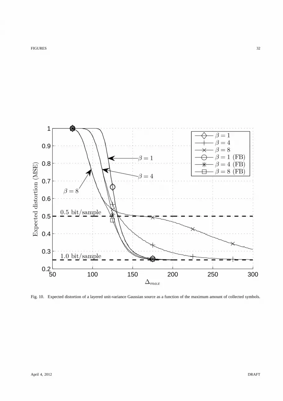
Finally, we present an evaluation where we map terminal states to distortion measures. We assume

that the decoded data describes a successive refinable [14] Gaussian source with unit variance, which

has been partitioned into two layers; base layer and refinement layer. It is assumed that if both

layers are decoded (LTB = LT

R = 0), 1 bit/sample is available to describe the source. If only the base

layer is decoded (LTB = 0, LT

R > 0), α bit/sample is available. If either no layers (LTB = LT

R > 0)

or the refinement layer only (LTB > 0, LT

R = 0) is decoded, we have0 bit/sample to describe the

source. This layered structure, which is common in e.g. video streaming, motivates the use of URT-

LT codes, since the base layer has more importance with respect to the distortion measure. For the

unit variance Gaussian source, we have thatD ≥ 2(−2R), whereD is the distortion measured as

the mean squared error andR is the rate measured in bits per sample. We assume that the bound

is achievable and use this relationship to calculate the expected distortion of the URT-LT codes

for both the case with acknowledgment of the base layer and the case without. The results are

shown in Fig. 10 for the same code parameters as in previous evaluations. The figure shows that

April 4, 2012 DRAFT

19

the optimal value ofβ depends on the overhead of the URT-LT code. Moreover, it is evident that

in the case of no acknowledgment of the base layer, if a low distortion is required at low overhead,

the price to pay is a very significant increase of the distortion at higher overhead. If the base layer

is acknowledged, the distortion quickly decreases to the minimum level, regardless of the choice

of β.

VI. CONCLUSIONS

We have analyzed finite-length LT codes with unequal recovery time, termed URT-LT codes

in this paper. The analysis is based on a state recursion function, which allows us to evaluate

the distributions of the ripple, cloud and decoding progress in individual segments, as the overall

decoding progresses. This gives novel insight into the probabilistic mechanisms in URT-LT codes,

which is a major contribution of this paper. The analysis enables us to evaluate the expected amount

of symbols with reduced degree0, i.e. redundant symbols, during a transmission. Evaluations in

the case of two data segments show that this amount increasesroughly linearly with the level of

priority given to the first data segment. As a result, successful decoding of the lower prioritized

data is delayed substantially. Thus, we can conclude that the unequal recovery time comes at a

significant price in terms of redundancy in lower prioritized data.

A slight modification of the URT-LT codes has been proposed, where an intermediate feedback

message informs the encoder that the higher prioritized data has been decoded. The encoder adapts

by excluding the decoded data from future encoding. Analysis of this code reveals that such a

modification is able to dramatically decrease the redundancy in lower prioritized data. The impact

of this improvement is further illustrated with an evaluation, where the decoding probabilities are

mapped to an expected distortion measure of a layered unit variance Gaussian source. Improvements

of roughly 0.25 in mean squared error is observed compared to the original URT-LT code.

APPENDIX

Proof of Theorem 1: Initially it is noted thatjjj follows Wallenius’ multivariate noncentral

hypergeometric distribution with parametersi, αααk andβββ. This distribution generalizes the hyper-

geometric distribution to take nonuniform sampling into account. For a certainjjj, the probability

of receiving a symbol with reduced degreei′i′i′ is found as a product ofN regular hypergeometric

distributions. This follows from the fact that a degree reduction from jn to i′n, n = 1, 2, ..., N ,

April 4, 2012 DRAFT

20

occurs wheni′n of the neighbors are among theℓn undecoded symbols and the remainingjn − i′n

neighbors are among theαnk−ℓn already decoded symbols. Sampling of neighbors within a single

layer is done uniformly, hence the hypergeometric distribution applies. Finally it is noted that any

symbol with jjj ∈ Ji can potentially reduce toi′i′i′ sincejn ≥ i′n, n = 1, 2, ..., N , and thatJi = ∅

unlessi′ ≤ i ≤ i′ + k − L.

Proof of Theorem 2: The probability of ending in the terminal statedddT , thus receiving the

next symbol in this state, when trying to decode the first∆ symbols, is given byfDDDT

(

dddT ,∆)

. The

expected number of symbols,E [∆dddT (∆max)], received in this state during an entire transmission

is found by summingfDDDT

(

dddT ,∆)

for all possible∆, i.e. ∆ = 1, ...,∆max. Of these, an expected

E [∆dddT (∆max)]π′β

(

000, ℓℓℓT)

have reduced degree0. Finally, the total amount of symbols,E [ǫ0k], with

reduced degree0 is found by summing over all terminal states in which the transmission continues,

i.e. any state in whichℓℓℓT 6= 000.

Proof of Theorem 3:The contribution from phase1,∑

dddT :ℓTB6=0 E

[

∆1dddT(∞)

]

π′β

(

000, ℓℓℓT)

, follows

the same structure as Theorem 2, although with a different condition for receiving more symbols,

since phase1 continues as long asℓTB 6= 0. The same holds for the contribution from phase2,∑

dddT :ℓTR6=0 E

[

∆2dddT(∞)

]

π′0

(

000, ℓℓℓT)

, although the amount of symbols received in phase2 is ∆2 −∆1

and the condition for receiving more symbols isℓTR 6= 0. See proof of Theorem 2 for details.

Proof of Lemma 1: If mn samples are drawn uniformly at random from a set of sizeℓn,

then the number of unique samples,q, will follow a distribution expressed by(ℓnq )Zq(mn)

(ℓn)mn, where

Zq(mn) =∑q

p=0

(

q

p

)

(q − p)mn(−1)p. This is an inverse variant of the coupon collector’s problem,

whose details can be found in []. Havingq unique released symbols, the number of those,m′n, who

are among theℓn − rn symbols not already in the ripple follows the hypergeometric distribution.

Having m′n ripple additions can be the result of any amount of unique releases higher thanm′

n.

Proof of Lemma 2: Since the next symbol to be processed is chosen uniformly at random

among the symbols in the ripple, the probability that it is a base layer symbol is the fraction of base

layer symbols currently in the ripple, rL+1

B

rL+1

B+rL+1

R

. Similarly, the probability that it is a refinement

layer symbol is rL+1

R

rL+1

B+rL+1

R

.

Proof of Lemma 3:Given a degreei, Φ(j, i, αk, β) expresses the probability of havingj base

layer symbols among thei neighbors. See proof of Theorem 1 for details. Assuming a base layer

symbol has just been processed, a symbol is released as a new base layer symbol whenℓB andℓR

April 4, 2012 DRAFT

21

symbols remain unprocessed from base layer and refinement layer respectively, ifj − 2 base layer

neighbors are among theαk − ℓB − 1 first processed base layer symbols, one is the(αk − ℓB)’th

processed base layer symbol, alli − j refinement layer neighbors are among the(1 − α)k − ℓR

processed refinement layer symbols and the last base layer neighbor is among theℓB undecoded

base layer symbols. This proves the expression forqBB(i, ℓℓℓL). Similar proofs can be made for

qBR(i, ℓℓℓL), qRB(i, ℓℓℓ

L) andqRR(i, ℓℓℓL).

Proof of Lemma 4:Any symbol with original degreei is released in the(k− L)’th decoding

step with prior probabilityq(

i, ℓℓℓL)

according to Lemma 3. All symbols with original degreei still

left in the cloud afterk−(L+1) decoding steps will release with conditional probabilityqc

(

i, ℓℓℓL)

=

q(i,ℓℓℓL)∑ℓL

RℓR=0

q(i,[0 ℓR])+∑ℓL

BℓB=1

q(i,[ℓB ℓLR])

, where the denominator expresses the remaining probability mass

of the prior probability distribution from Lemma 3. Hence, the amount of degreei symbols,M Li ,

released in the next decoding step, follows the binomial distribution, θ(

mLi , c

L+1i , qc

(

i, ℓℓℓL))

. The

probability of having a cloud ofcccL after that decoding step is thus found as a product of binomial

distributions, evaluated atmLi , ∀ i.

Proof of Lemma 5:For a certain cloud development in the(k− L)’th decoding step, the total

amount of releases,mL, is found asmL =∑k

i=2 cL+1i − cLi . These releases are differentiated among

layers using equation (6), thereby achievingmLB and mL

B = mL − mLB. Lemma 1 is then used to

express the distributions of the amounts,M L′

B andM L′

R , which are added to the ripple.

REFERENCES

[1] M. Luby, “LT Codes,” in Proceedings. The 43rd Annual IEEE Symposium on Foundationsof Computer Science., pp. 271–280,

November 2002.

[2] A. Shokrollahi, “Raptor codes,”IEEE Transactions on Information Theory., pp. 2551–2567, 2006.

[3] Y. Cao, S. Blostein, and W.-Y. Chan, “Optimization of rateless coding for multimedia multicasting,” inBroadband Multimedia

Systems and Broadcasting (BMSB), 2010 IEEE International Symposium on, pp. 1–6, March 2010.

[4] K. Nybom, S. Gronroos, and J. Bjorkqvist, “Expanding window fountain coded scalable video in broadcasting,” inMultimedia

and Expo (ICME), 2010 IEEE International Conference on, pp. 516–521, July 2010.

[5] S. Karande, K. Misra, S. Soltani, and H. Radha, “Design and analysis of generalized lt-codes using colored ripples,”in

Information Theory, 2008. ISIT 2008. IEEE International Symposium on, pp. 2071–2075, July 2008.

[6] M. Bogino, P. Cataldi, M. Grangetto, E. Magli, and G. Olmo, “Sliding-window digital fountain codes for streaming of

multimedia contents,” inCircuits and Systems, 2007. ISCAS 2007. IEEE InternationalSymposium on, pp. 3467–3470, May

2007.

April 4, 2012 DRAFT

22

[7] D. Sejdinovic, D. Vukobratovic, A. Doufexi, V.Senk, and R. Piechocki, “Expanding window fountain codes for unequal error

protection,”Communications, IEEE Transactions on, vol. 57, pp. 2510 –2516, september 2009.

[8] H. Neto, W. Henkel, and V. da Rocha, “Multi-edge framework for unequal error protecting lt codes,” inInformation Theory

Workshop (ITW), 2011 IEEE, pp. 267–271, October 2011.

[9] N. Rahnavard, B. Vellambi, and F. Fekri, “Rateless codeswith unequal error protection property,”Information Theory, IEEE

Transactions on, vol. 53, pp. 1521–1532, April 2007.

[10] P. Cataldi, M. Grangetto, T. Tillo, E. Magli, and G. Olmo, “Sliding-window raptor codes for efficient scalable wireless video

broadcasting with unequal loss protection,”Image Processing, IEEE Transactions on, vol. 19, pp. 1491–1503, June 2010.

[11] R. Karp, M. Luby, and A. Shokrollahi, “Finite length analysis of lt codes,” inInformation Theory, 2004. ISIT 2004. Proceedings.

International Symposium on, p. 39, June/July 2004.

[12] N. Rahnavard, B. N. Vellambi and F. Fekri, “Rateless Codes With Unequal Error Protection Property,”IEEE Transactions on

Information Theory vol. 53., pp. 1521 – 1532, April 2007.

[13] D. MacKay, “Fountain codes,”Communications, IEE Proceedings-, vol. 152, pp. 1062 – 1068, December 2005.

[14] T. Cover and J. Thomas,Elements of information theory. New York: Wiley, 1991.

April 4, 2012 DRAFT

FIGURES 23

1 2 3 4 5 6 7 8 9 10

1 2 3 4 5 6 7 8 9 10

15 792 468 3 10

11 12 13

Input symbols

Output symbols

Order of processing:

Degree: 2 3 2 4 7 1 2 1 4 1 2 1 1

Fig. 1. Graph representation of the example code.

April 4, 2012 DRAFT

FIGURES 24

0 1 2 3 4 5 60

1

2

3

4

L1

L2

Initial State

Terminal State

Fig. 2. An example of a decoder state evolution with two terminal states before successful decoding.

April 4, 2012 DRAFT

FIGURES 25

010

2030

4050

010

2030

4050

0

0.2

0.4

0.6

0.8

1

ℓTB

ℓTR

π′ β(0

,ℓT

)

Fig. 3. The probability of receiving a symbol with reduced degree zero,π′β (000, ℓℓℓ), for a two-layer LT code with parametersα = 0.5,

β = 9 andk = 100.

April 4, 2012 DRAFT

FIGURES 26

LT B

LTR

β =1

50 40 30 20 10 0

0

10

20

30

40

50

LT B

LTR

β =4

50 40 30 20 10 0

0

10

20

30

40

50

LT B

LTR

β =16

50 40 30 20 10 0

0

10

20

30

40

50

LT B

LTR

β =32

50 40 30 20 10 0

0

10

20

30

40

50

0.0000

0.0000

0.0003

0.0025

0.0183

0.1353

Fig. 4. NormalizedE [∆dddT ] as a function ofLTB andLT

R at different values ofβ.

April 4, 2012 DRAFT

FIGURES 27

LT B

LTR

50 40 30 20 10 0

0

5

10

15

20

25

30

35

40

45

50

Fig. 5. Actual simulations of the analyzed URT-LT code illustrated on top of the analytical results.

April 4, 2012 DRAFT

FIGURES 28

50 100 150 2000

0.1

0.2

0.3

0.4

0.5

0.6

0.7

0.8

0.9

1

∆max

Pr(L

T B=

0)

β = 1β = 4β = 8

Fig. 6. Probability of successfully decoding the base layeras a function of the maximum amount of collected symbols.

April 4, 2012 DRAFT

FIGURES 29

0 200 400 600 800 1000 1200 1400 1600 18000

100

200

300

400

500

600

∆max

E[k

ǫ 0(∆

max)]

β = 1β = 2β = 4β = 8β = 16β = 24β = 32

Fig. 7. Expected amount of redundancy due to reduced degree zero as a function of the maximum amount of collected symbolsfor different values ofβ in the case of no feedback.

April 4, 2012 DRAFT

FIGURES 30

0 50 100 150 2000

5

10

15

20

25

∆max

E[

kǫF 0

(∆m

ax)]

β = 1β = 2β = 4β = 8β = 16β = 24β = 32β = 48

Fig. 8. Expected amount of redundancy due to reduced degree zero as a function of the maximum amount of collected symbolsfor different values ofβ in the case of feedback.

April 4, 2012 DRAFT

FIGURES 31

0 10 20 30 40 5010

0

101

102

103

E[k

ǫ 0(∞

)]/

E[

kǫF 0

(∞)]

β

Without FBWith FB

Fig. 9. Asymptotic values ofE [kǫ0(∆max)] andE[

kǫF0 (∆max)]

as a function ofβ.

April 4, 2012 DRAFT

FIGURES 32

50 100 150 200 250 3000.2

0.3

0.4

0.5

0.6

0.7

0.8

0.9

1

0.5 bit/sample

1.0 bit/sample

∆max

Expec

ted

dis

tort

ion

(MSE

)

β = 1β = 4β = 8β = 1 (FB)β = 4 (FB)β = 8 (FB)

β = 8

β = 4

β = 1

Fig. 10. Expected distortion of a layered unit-variance Gaussian source as a function of the maximum amount of collectedsymbols.

April 4, 2012 DRAFT

TABLES 33

TABLE IEXAMPLE OF A DECODER STATE EVOLUTION.

k − L L1 L2 R1 R2 C2 C3 C4 C5 C6 C7 C8 C9 C10

0 6 4 2 1 3 1 2 0 0 1 0 0 01 5 4 1 1 3 1 2 0 0 1 0 0 02 4 4 0 1 3 1 2 0 0 1 0 0 03 4 3 0 0 3 1 2 0 0 1 0 0 0

3 4 3 1 0 4 1 2 0 0 1 0 0 04 3 3 2 0 2 1 2 0 0 1 0 0 05 2 3 1 0 2 1 2 0 0 1 0 0 06 1 3 0 0 2 1 2 0 0 1 0 0 0

6 1 3 0 1 2 1 2 0 0 1 0 0 07 1 2 1 0 2 0 2 0 0 1 0 0 08 0 2 0 2 0 0 1 0 0 1 0 0 09 0 1 0 1 0 0 0 0 0 0 0 0 010 0 0 0 0 0 0 0 0 0 0 0 0 0

April 4, 2012 DRAFT