Decipherability of codes

Journal of Pure and Applied Algebra 141 (1999) 13–35www.elsevier.com/locate/jpaa

Decipherability of codesFernando Guzm�an

Department of Mathematical Sciences, SUNY, Binghamton, NY 13902-6000, USA

Communicated by J. Rhodes; received 26 June 1995; received in revised form 5 November 1997

Abstract

Several forms of decipherability of codes, like unique decipherability, multiset decipherabilityand set decipherability are subsumed under a general concept of decipherability using varieties ofmonoids. A Galois connection is established between classes of codes and varieties of monoids,establishing a measure of the decipherability of a class of codes. Several well-known classes ofcodes are shown to be varieties, and several varieties of monoids are shown to be codi�able.Examples are also given of non-codi�able varieties of monoids. The simpli�ed domino graph ofa code is constructed, and it is shown that the language it accepts forms a basis for the varietyof monoids associated with the code. c© 1999 Elsevier Science B.V. All rights reserved.

MSC: 94A45; 20M07; 08B15; 68R15; 06B99

When a source message is encoded using a uniquely decipherable code, UD forshort, the deciphering process will recover the original message in its entirety. This isthe de�ning property of unique decipherability. There are situations, however, when itis not desirable or necessary to recover the whole original message, but only part of theinformation embedded in it. In these cases, something weaker than unique decipher-ability is the appropriate property for a code to have. One of these weaker conceptsis that of multiset decipherability, MSD for short, introduced by Lempel in [8] andfurther explored by Restivo in [11] and by Head and Weber in [6]. In this case the de-ciphering process recovers the original message up to a permutation of the codewords,i.e., up to commutativity. In other words, the original message itself is not alwaysrecovered, but the multiset of code words that form it is. As pointed out in [8], acouple of situations where multiset decipherability is su�cient, are in the transmissionof information for the construction of histograms and in compiling an inventory; wewill use this last situation as our standard example in the next couple of paragraphs.Obviously there are situations where this form of decipherability is not only su�cient,but also desirable, if the additional information is to be kept concealed.

0022-4049/99/$ - see front matter c© 1999 Elsevier Science B.V. All rights reserved.PII: S0022 -4049(98)00019 -X

14 F. Guzm�an / Journal of Pure and Applied Algebra 141 (1999) 13–35

We introduce in this paper a very similar concept, that of set decipherability, SDfor short. In this case the original message is recovered up to commutativity andactual count of occurrences. This may be useful for example in the case of two rivalparties willing to inform each other of the presence or absence of certain items in theirinventories, without revealing the exact count.Another form of transmitting only partial information about the inventory is with the

use of numerically decipherable codes, ND for short, introduced by Weber and Headin [13]. In this case only the total number of items in the inventory can be recovered,but not their type.We propose to measure the decipherability of a code or a class of codes using va-

rieties of monoids. When we say that a message encoded with a MSD code can berecovered up to commutativity, what we are saying is that MSD codes can be deci-phered over commutative monoids. Of the four examples of decipherability mentionedabove, UD, MSD, SD, and ND, the �rst three are particular cases of this more generalconcept of decipherability in monoids; see Propositions 1.1, 1.2 and 2.3. Unfortunately,the last one does not �t into this scheme; see Proposition 2.11. This suggests that aneven more general study of decipherability should be attempted.The connection between codes and monoids is established using the simpli�ed

domino graph of a code. This is a minor variation on the domino graph of a code usedin [6, 13], and by Weber in [12]. From our point of view the simpli�ed domino graphof a code is an improvement over the domino graph, because it eliminates duplicityin the relations read from the graph, as well as trivial relations. We believe many ofthe results of Head and Weber can be expressed, and sometimes with fewer technicalrestrictions, using the simpli�ed domino graph.The concept of decipherability that we introduce, establishes a Galois connection

between certain classes of codes, varieties of codes, and certain varieties of monoids,codi�able varieties of monoids. Our hope is that this connection will allow the use ofknowledge about monoids to better understand decipherability of codes; at the sametime allowing the use of codes to explore problems connected with the lattice ofvarieties of monoids.In Section 1 we introduce the concept of decipherability, show that UD and MSD

are special cases of it and establish the Galois connection between classes of codes andclasses of monoids; see Theorem 1.5. We also show that the concept of decipherabilityis alphabet independent, and therefore one can work over a two letter alphabet, withoutany loss of generality. In Section 2 we give some examples of varieties of codes, aswell as codi�able and non-codi�able varieties of monoids. In particular we show thatUD, MSD and SD are varieties of codes, whereas the variety of Abelian monoidsand the variety of semilattices are codi�able. We also show that the class of NDcodes is not a variety of codes. In Section 3 we construct the simpli�ed dominograph of a code, and show that the language accepted by this graph when treatedas an automaton, is a basis of identities for the variety of monoids where the code isdecipherable; see Theorem 3.3. In other words, one can read one direction of the Galoisconnection from the simpli�ed domino graph. In Section 4 we show that all varieties

F. Guzm�an / Journal of Pure and Applied Algebra 141 (1999) 13–35 15

of commutative monoids are codi�able, and as a consequence the lattice of varietiesof codes contains a complete sublattice anti-isomorphic to the lattice of non-negativeintegers under divisibility; see Theorem 4.1 and Corollary 4.2. We believe this is asmall �rst step in the process of describing the lattice of varieties of codes.

1. Decipherability of codes in monoids

Throughout this paper A will denote an alphabet, i.e., a �nite non-empty set, A∗ thefree monoid on A, consisting of all words over A, including the empty word �, andA+ = A∗−{�}. By a code over A we mean a �nite subset C of A+. We denote by C∗

the submonoid of A∗ generated by C. It consists of all words which are concatenationof code words. The elements of C∗ are called messages. Note that C∗ is not necessarilyfreely generated by C; see Proposition 1.1 below. In fact, it does not even have to bea free monoid. For background material on codes we refer the reader to Ad�amek [1]and Berstel and Perrin [2]. For background material on universal algebra we refer toBurris and Sankappanavar [3].Given a code C and a monoid M , we say that C is decipherable in M if every map

f :C→M extends to a (unique) homomorphism f :C∗ →M . In other words, if underany interpretation f of the code words in M , every message has a unique meaning.A code C is said to be uniquely decipherable (UD for short), if every message has

a unique factorization into code words. The following proposition includes well-knownfacts about free monoids, written here in terms of decipherability to illustrate the factthat unique decipherability is a special case of decipherability as de�ned above.

Proposition 1.1. Let C be a code; and F the free monoid in 2 generators. Thefollowing are equivalent:(1) C is UD.(2) C is decipherable in every monoid.(3) C is decipherable in F.(4) C∗ is freely generated by C.

Proof. (1)⇔ (4)⇔ (2) is a well-known fact about free monoids written here in termsof decipherability.(2)⇒ (3) is obvious.(3)⇒ (1): Let C = {c1; : : : ; ck} be a code which is decipherable in F the free monoid

in two generators a and b. Suppose C is not UD. Let u∈C∗ be the shortest messagewith two distinct factorizations, u= ci1 · · · cin = cj1 · · · cjm . By the choice of u we haveci1 6= cj1 , and the map f :C→F de�ned by f(ci1 ) = a, f(cj1 ) = b and f(cl)= � forcl ∈C−{ci1 ; cj1} does not extend to C∗.

A code C is said to be multiset decipherable (MSD for short), if for any messageu∈C∗, all factorizations of u over C yield the same multiset of code words [8]. Thefollowing proposition shows that MSD is also a special case of decipherability.


Proposition 1.2. Let C be a code; and N the monoid of natural numbers under ad-dition. The following are equivalent:(1) C is MSD.(2) C is decipherable in every Abelian monoid.(3) C is decipherable in N.

Proof. (1)⇒ (2): Suppose C = {c1; : : : ; ck} is MSD. Let M be an Abelian monoid andf :C→M a map. If u∈C∗ is a message over C that factors as u= ci1 · · · cin = cj1 · · ·cjm , then C being MSD implies equality of the multisets {ci1 ; : : : ; cin} and {cj1 ; : : : ; cjm}.M being Abelian implies that f(ci1 ) · · ·f(cin)=f(cj1 ) · · ·f(cjm) so we just set f(u)=f(ci1 ) · · ·f(cin).(2)⇒ (3) is obvious.(3)⇒ (1): Suppose C = {c1; : : : ; ck} is decipherable in N. Consider the maps

fi :C→N for i=1; : : : ; k, given by fi(cj)= �i; j. By hypothesis, fi extends to C∗,and for u∈C∗, fi(u) is the number of times ci occurs in any factorization of u. There-fore any two factorizations of u involve the same number of occurrences of ci. Sincethis holds for every i=1; : : : ; k; C is MSD.

The equivalence of (1) and (2) in Propositions 1.1 and 1.2 suggests that we lookat the class of monoids a given code is decipherable in. More generally, for K aclass of codes let M(K) denote the class of monoids M such that every C ∈K isdecipherable in M . For V a class of monoids, let C(V ) be the class of codes C whichare decipherable in every M ∈V . When K is a singleton K = {C}, we will denoteM({C}) by M(C). Similarly C(M) denotes C({M}).Note that M(K)=

⋂C∈K M(C), and C(V )=

⋂M∈V C(M). Moreover, M ∈M(C)

i� C ∈C(M).

Proposition 1.3. Let K be a class of codes. M(K) is a variety of monoids.

Proof. Since M(K)=⋂C∈K M(C), it su�ces to show that for a code C, M(C) is a

variety. That is what we prove in the next lemma.

Let C be a code, and consider the code words in an arbitrary but �xed order C ={c1; : : : ; ck}. Let B be an alphabet, disjoint from A, and with the same cardinalityas C. Consider the letters of B also in an arbitrary but �xed order B= {b1; : : : ; bk}.We will refer to B as the alphabet of relations of C. Let �; �∈B∗. We say that Csatis�es the relation �∼ � if �(c1; : : : ; ck)= �(c1; : : : ; ck) where �(c1; : : : ; ck) is obtainedfrom � by substituting ci for bi, i=1; : : : ; k. A monoid M satis�es the identity �≈ � if�(m1; : : : ; mk)= �(m1; : : : ; mk) for every m1; : : : ; mk ∈M ; see [3, Section III.11.1]. Whenrefering to varieties of monoids de�ned by identities, the monoid identities, associativityand identity element, will be implicitly assumed. When writing identities we will use1 instead of �. For example, the variety of groups of n-bounded exponent is de�nedby the identity xn≈ � that we will write as xn≈ 1.


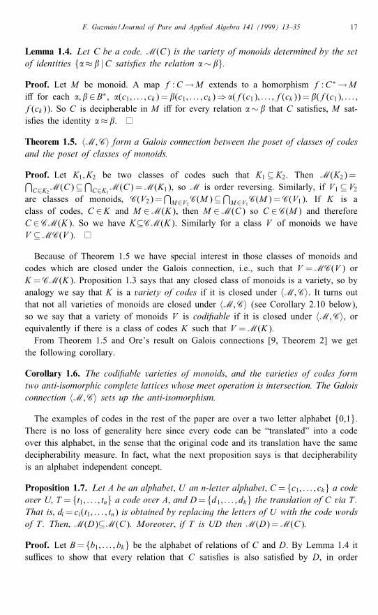
Lemma 1.4. Let C be a code. M(C) is the variety of monoids determined by the setof identities {�≈ � |C satis�es the relation �∼ �}.

Proof. Let M be monoid. A map f :C→M extends to a homorphism f :C∗ →Mi� for each �; �∈B∗, �(c1; : : : ; ck)= �(c1; : : : ; ck)⇒ �(f(c1); : : : ; f(ck))= �(f(c1); : : : ;f(ck)). So C is decipherable in M i� for every relation �∼ � that C satis�es, M sat-is�es the identity �≈ �.

Theorem 1.5. 〈M;C〉 form a Galois connection between the poset of classes of codesand the poset of classes of monoids.

Proof. Let K1; K2 be two classes of codes such that K1⊆K2. Then M(K2)=⋂C∈K2M(C)⊆⋂C∈K1M(C)=M(K1), so M is order reversing. Similarly, if V1⊆V2

are classes of monoids, C(V2)=⋂M∈V2C(M)⊆

⋂M∈V1C(M)=C(V1). If K is a

class of codes, C ∈K and M ∈M(K), then M ∈M(C) so C ∈C(M) and thereforeC ∈CM(K). So we have K⊆CM(K). Similarly for a class V of monoids we haveV ⊆MC(V ).

Because of Theorem 1.5 we have special interest in those classes of monoids andcodes which are closed under the Galois connection, i.e., such that V =MC(V ) orK =CM(K). Proposition 1.3 says that any closed class of monoids is a variety, so byanalogy we say that K is a variety of codes if it is closed under 〈M;C〉. It turns outthat not all varieties of monoids are closed under 〈M;C〉 (see Corollary 2.10 below),so we say that a variety of monoids V is codi�able if it is closed under 〈M;C〉, orequivalently if there is a class of codes K such that V =M(K).From Theorem 1.5 and Ore’s result on Galois connections [9, Theorem 2] we get

the following corollary.

Corollary 1.6. The codi�able varieties of monoids; and the varieties of codes formtwo anti-isomorphic complete lattices whose meet operation is intersection. The Galoisconnection 〈M;C〉 sets up the anti-isomorphism.

The examples of codes in the rest of the paper are over a two letter alphabet {0,1}.There is no loss of generality here since every code can be “translated” into a codeover this alphabet, in the sense that the original code and its translation have the samedecipherability measure. In fact, what the next proposition says is that decipherabilityis an alphabet independent concept.

Proposition 1.7. Let A be an alphabet; U an n-letter alphabet; C = {c1; : : : ; ck} a codeover U; T = {t1; : : : ; tn} a code over A; and D= {d1; : : : ; dk} the translation of C via T .That is; di= ci(t1; : : : ; tn) is obtained by replacing the letters of U with the code wordsof T . Then; M(D)⊆M(C). Moreover; if T is UD then M(D)=M(C).

Proof. Let B= {b1; : : : ; bk} be the alphabet of relations of C and D. By Lemma 1.4 itsu�ces to show that every relation that C satis�es is also satis�ed by D, in order


to get the �rst inclusion. Let �; �∈B∗ and suppose that C satis�es the relation �∼ �.Then �(c1; : : : ; ck)= �(c1; : : : ; ck), and if we replace each letter ui of U with the cor-responding code word ti of T , we get �(d1; : : : ; dk)= �(d1; : : : ; dk), so D satis�esthe relation �∼ �. Assume now that T is UD and D satis�es the relation �∼ �.Then �(d1; : : : ; dk)= �(d1; : : : ; dk), that is �(c1(t1; : : : ; tn); : : : ; ck(t1; : : : ; tn))=�(c1(t1; : : : ; tn); : : : ; ck(t1; : : : ; tn)). Since T is a UD code, it follows that �(c1; : : : ; ck)=�(c1; : : : ; ck), that is, C satis�es �∼ �.

Over a non-trivial alphabet A (|A| ≥ 2) there are UD codes of arbitrary size. Forexample, for every n≥ 1, An is a UD code. Therefore, any code can be translated intoa code over a non-trivial alphabet, preserving the decipherability.

2. Examples: varieties of codes. Codi�able varieties of monoids

In this section we will use the Galois connection 〈M;C〉, to show the correspondencebetween some well known classes of codes and some familiar varieties of monoids.We will also use it to give examples of non-codi�able varieties of monoids.Let UD stand for the class of all uniquely decipherable codes, and MSD for the

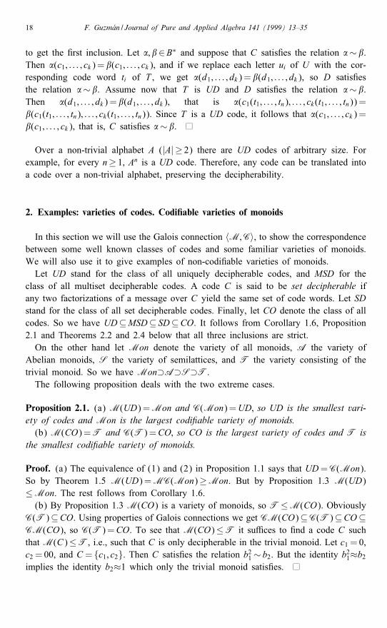
class of all multiset decipherable codes. A code C is said to be set decipherable ifany two factorizations of a message over C yield the same set of code words. Let SDstand for the class of all set decipherable codes. Finally, let CO denote the class of allcodes. So we have UD⊆MSD⊆ SD⊆CO. It follows from Corollary 1.6, Proposition2.1 and Theorems 2.2 and 2.4 below that all three inclusions are strict.On the other hand let Mon denote the variety of all monoids, A the variety of

Abelian monoids, S the variety of semilattices, and T the variety consisting of thetrivial monoid. So we have Mon⊃A⊃S⊃T.The following proposition deals with the two extreme cases.

Proposition 2.1. (a) M(UD)=Mon and C(Mon)=UD; so UD is the smallest vari-ety of codes and Mon is the largest codi�able variety of monoids.(b) M(CO)=T and C(T)=CO; so CO is the largest variety of codes and T is

the smallest codi�able variety of monoids.

Proof. (a) The equivalence of (1) and (2) in Proposition 1.1 says that UD=C(Mon).So by Theorem 1.5 M(UD)=MC(Mon)≥Mon. But by Proposition 1.3 M(UD)≤Mon. The rest follows from Corollary 1.6.(b) By Proposition 1.3 M(CO) is a variety of monoids, so T≤M(CO). Obviously

C(T)⊆CO. Using properties of Galois connections we get CM(CO)⊆C(T)⊆CO⊆CM(CO), so C(T)=CO. To see that M(CO)≤T it su�ces to �nd a code C suchthat M(C)≤T, i.e., such that C is only decipherable in the trivial monoid. Let c1 = 0,c2 = 00, and C = {c1; c2}. Then C satis�es the relation b21∼ b2. But the identity b21≈b2implies the identity b2≈1 which only the trivial monoid satis�es.


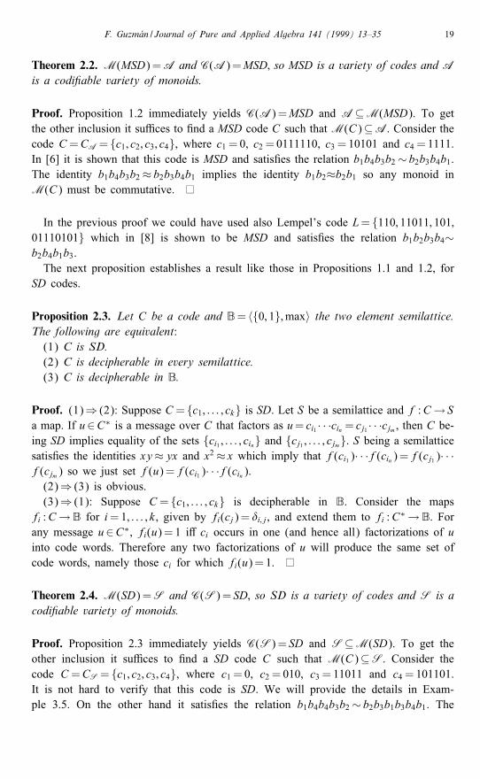
Theorem 2.2. M(MSD)=A and C(A)=MSD; so MSD is a variety of codes and A

is a codi�able variety of monoids.

Proof. Proposition 1.2 immediately yields C(A)=MSD and A⊆M(MSD). To getthe other inclusion it su�ces to �nd a MSD code C such that M(C)⊆A. Consider thecode C =CA= {c1; c2; c3; c4}, where c1 = 0, c2 = 0111110, c3 = 10101 and c4 = 1111.In [6] it is shown that this code is MSD and satis�es the relation b1b4b3b2∼ b2b3b4b1.The identity b1b4b3b2≈ b2b3b4b1 implies the identity b1b2≈b2b1 so any monoid inM(C) must be commutative.

In the previous proof we could have used also Lempel’s code L= {110; 11011; 101;01110101} which in [8] is shown to be MSD and satis�es the relation b1b2b3b4∼b2b4b1b3.The next proposition establishes a result like those in Propositions 1.1 and 1.2, for

SD codes.

Proposition 2.3. Let C be a code and B= 〈{0; 1};max〉 the two element semilattice.The following are equivalent:(1) C is SD.(2) C is decipherable in every semilattice.(3) C is decipherable in B.

Proof. (1)⇒ (2): Suppose C = {c1; : : : ; ck} is SD. Let S be a semilattice and f :C→ Sa map. If u∈C∗ is a message over C that factors as u= ci1 · · ·cin = cj1 · · ·cjm , then C be-ing SD implies equality of the sets {ci1 ; : : : ; cin} and {cj1 ; : : : ; cjm}. S being a semilatticesatis�es the identities xy≈yx and x2≈ x which imply that f(ci1 )· · ·f(cin)=f(cj1 )· · ·f(cjm) so we just set f(u)=f(ci1 )· · ·f(cin).(2)⇒ (3) is obvious.(3)⇒ (1): Suppose C = {c1; : : : ; ck} is decipherable in B. Consider the maps

fi :C→B for i=1; : : : ; k, given by fi(cj)= �i; j, and extend them to fi :C∗ →B. Forany message u∈C∗, fi(u)= 1 i� ci occurs in one (and hence all) factorizations of uinto code words. Therefore any two factorizations of u will produce the same set ofcode words, namely those ci for which fi(u)= 1.

Theorem 2.4. M(SD)=S and C(S)= SD; so SD is a variety of codes and S is acodi�able variety of monoids.

Proof. Proposition 2.3 immediately yields C(S)= SD and S⊆M(SD). To get theother inclusion it su�ces to �nd a SD code C such that M(C)⊆S. Consider thecode C =CS= {c1; c2; c3; c4}, where c1 = 0, c2 = 010, c3 = 11011 and c4 = 101101.It is not hard to verify that this code is SD. We will provide the details in Exam-ple 3.5. On the other hand it satis�es the relation b1b4b4b3b2∼ b2b3b1b3b4b1. The


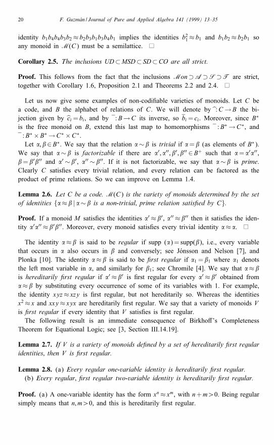
identity b1b4b4b3b2≈ b2b3b1b3b4b1 implies the identities b21≈ b1 and b1b2≈ b2b1 soany monoid in M(C) must be a semilattice.

Corollary 2.5. The inclusions UD⊂MSD⊂ SD⊂CO are all strict.

Proof. This follows from the fact that the inclusions Mon⊃A⊃S⊃T are strict,together with Corollary 1.6, Proposition 2.1 and Theorems 2.2 and 2.4.

Let us now give some examples of non-codi�able varieties of monoids. Let C bea code, and B the alphabet of relations of C. We will denote by :C→B the bi-jection given by ci= bi, and by :B→C its inverse, so bi= ci. Moreover, since B∗

is the free monoid on B, extend this last map to homomorphisms :B∗ →C∗, and:B∗ ×B∗ →C∗ ×C∗.Let �; �∈B∗. We say that the relation �∼ � is trivial if �= � (as elements of B∗).

We say that �∼ � is factorizable if there are �′; �′′; �′; �′′ ∈B+ such that �= �′�′′,�= �′�′′ and �′ ∼ �′, �′′ ∼ �′′. If it is not factorizable, we say that �∼ � is prime.Clearly C satis�es every trivial relation, and every relation can be factored as theproduct of prime relations. So we can improve on Lemma 1.4.

Lemma 2.6. Let C be a code. M(C) is the variety of monoids determined by the setof identities {�≈ � | �∼ � is a non-trivial; prime relation satis�ed by C}.

Proof. If a monoid M satis�es the identities �′ ≈ �′, �′′ ≈ �′′ then it satis�es the iden-tity �′�′′ ≈ �′�′′. Moreover, every monoid satis�es every trivial identity �≈ �.

The identity �≈ � is said to be regular if supp (�)= supp(�), i.e., every variablethat occurs in � also occurs in � and conversely; see J�onsson and Nelson [7], andPlonka [10]. The identity �≈ � is said to be �rst regular if �1 = �1 where �1 denotsthe left most variable in �, and similarly for �1; see Chromile [4]. We say that �≈ �is hereditarily �rst regular if �′ ≈ �′ is �rst regular for every �′ ≈ �′ obtained from�≈ � by substituting every occurrence of some of its variables with 1. For example,the identity xyz≈ xzy is �rst regular, but not hereditarily so. Whereas the identitiesx2≈ x and xxy≈ xyx are hereditarily �rst regular. We say that a variety of monoids Vis �rst regular if every identity that V satis�es is �rst regular.The following result is an immediate consequence of Birkho�’s Completeness

Theorem for Equational Logic; see [3, Section III.14.19].

Lemma 2.7. If V is a variety of monoids de�ned by a set of hereditarily �rst regularidentities; then V is �rst regular.

Lemma 2.8. (a) Every regular one-variable identity is hereditarily �rst regular.(b) Every regular; �rst regular two-variable identity is hereditarily �rst regular.

Proof. (a) A one-variable identity has the form xn≈ xm, with n+m¿0. Being regularsimply means that n; m¿0, and this is hereditarily �rst regular.


(b) If �≈ � is a regular, �rst regular two-variable identity then substituting one of thevariables with 1 yields a regular one-variable identity and by part (a) it is hereditarily�rst regular.

The identities x2≈ x and xxy≈ xyx are examples of (a) and (b), respectively.

Theorem 2.9. Let V be a �rst regular; proper variety of monoids. Then V is notcodi�able.

Proof. We know from Proposition 2.1(a) that UD≤C(V ). Let us show that in factC(V )=UD. Let C be a non-UD code. Then C satis�es some non-trivial, prime relation�∼ �. By Lemma 2.6 M(C) satis�es �≈ �. Since �∼ � is prime and non-trivial, �≈ �is not �rst regular, and therefore V 6≤ M(C). So C =∈C(V ), and we have C(V )≤UD.It follows that MC(V )=M(UD). By Proposition 2.1(a), and the hypothesis of Vbeing proper, MC(V )=Mon 6=V , so V is not codi�able.

Note that the appropriate de�nitions and arguments symmetric to those used inLemmas 2.7, 2.8 and Theorem 2.9 yield

Theorem 2.9′. Let V be a last regular; proper variety of monoids. Then V is notcodi�able.

Corollary 2.10. (a) The variety of monoids de�ned by the identity xn≈ xm wheren¿m≥ 1 is not codi�able. In particular the variety of bands with unity which isde�ned by the identity x2≈ x is not codi�able.(b) Let � 6= �∈{x; y}∗ be such that y∈ supp(�)∩ supp(�). The variety of monoids

de�ned by x�≈ x� is not codi�able. In particular the variety of monoids de�ned bythe identity xxy≈ xyx is not codi�able.

Proof. Follows from Lemmas 2.8, 2.7 and Theorem 2.9. Note that V is a propervariety, by the hypotheses n 6=m, and � 6=� in (a) and (b) respectively.

Note that the variety of monoids de�ned by xxy≈ xyx contains A, whereas thevariety of bands with unity is not comparable to A. Contrast this with Theorem 4.1below.Let us close this section showing that the class ND of numerically decipherable codes

is not a variety. Recall from [13] that a code is said to be numerically decipherable ifany two factorizations of a message over the code involve the same number of codewords, counting multiplicity.

Proposition 2.11. The class ND of numerically decipherable codes is not a varietyof codes.

Proof. The class ND is a proper class of codes. For example the code {0; 00} is notND. So it su�ces to �nd a ND code C such that M(C)=T. Consider the code


C = {0; 10; 01}. It is easy to verify that the only non-trivial prime relations that Csatis�es are the relations b1bn2∼ bn3b1 for n≥ 1. So C is ND. Let M be a monoid suchthat M ∈M(C). By Lemma 2.6, taking n=1 we have that M satis�es the identityxy≈ zx. Thus, it satis�es y≈ z; and M is trivial.

3. Codes and their relations

In order to study the relations satis�ed by a code C, we will look at the simpli�eddomino graph and the domino function of C. This is a minor variation on the dominogroup of a code used in [6] to decide multiset decipherability. In fact, the simpli�eddomino graph of C is a subgraph of the Head–Weber domino graph of C, but stillgives us the information about decipherability of C as it is shown in Theorem 3.3below.For two words u; v over the same alphabet, we will write u≤p v to indicate that u

is a pre�x of v, and u¡p v to indicate that u≤p v and u 6= v. If u≤p v then we denoteby u−1v the su�x w of v such that v= uw, and call it their balance.Let P=Pre�x(C) denote the set of all pre�xes of words in C. Let G=(V ; E) be

the directed graph having as vertex set

V = {open,close}∪ {(u; �) | u∈P−{�}}∪ {(�; u) | u∈P−{�}}

and as edge set E=E1 ∪E2 ∪E3 ∪E4 where

E1 = {(open; (�; u)) | u∈C};

E2 = {((u; �); close) | u∈C};

E3 = {((u; �); (uv; �)) | v∈C}∪ {((�; u); (�; uv)) | v∈C};

E4 = {((u; �); (�; v)) | uv∈C}∪ {((�; u); (v; �)) | uv∈C}:

Notice that the edges in E3 and E4 come in symmetric pairs: ((u; �); (uv; �)) with((�; u); (�; uv)) and ((u; �); (�; v)) with ((�; u); (v; �)), each one being the mirror imageof the other. In Section 4 below when we list the type E3 and E4 edges of G fora particular C, we will only list half of them, and refer to the other half as theirsymmetric images.Recall from Section 2 that :C→B is the bijection from the code to the alphabet

of relations, and :B→C its inverse. The domino function associated with C is themap d : E→B×{�}∪ {�}×B de�ned– on E1 by d(open; (�; u))= ( u; �),– on E2 by d((u; �); close)= ( u; �),– on E3 by d((u; �); (uv; �))= (�; v) and d((�; u); (�; uv))= ( v; �),– on E4 by d((u; �); (�; v))= (uv; �) and d((�; u); (v; �))= (�; uv).


The pair d(e) is called the domino associated with edge e of G. The domino functionis extended to paths in a standard way. If p is the path in G consisting of edgese1; e2; : : : ; em; in that order, we de�ne d(p)=d(e1)·d(e2) · · ·d(em)∈B∗ ×B∗. The pair(�; �)∈B∗ ×B∗ will often be written as [�

�].

Let V consist of open,close and those w∈ V such that there is a path from open

to close that goes through w. Let E consists of those e∈ E such that there is a pathfrom open to close that goes through e. The graph G=G(C)= (V; E) is called thesimpli�ed domino graph of C. We call the elements of V biaccessible vertices in G,i.e., accessible from open and coaccessible from close. The elements of E are calledbiaccessible edges in G.The next two lemmas illustrate how the paths from open to close in G correspond

to non-trivial prime relations satis�ed by C.Let �=�C∗ = {(u; u) | u∈C∗}. Observe that except for open and close, all other

vertices in V are elements of P×P. In the next lemma, to simplify the notation, wewill identify both open and close with (�; �). This identi�cation is natural if we thinkof a path from open to a vertex w, as the beginning of an ambiguous factorization of amessage: each edge adds a codeword to one of the two meanings, top or bottom; eachvertex, keeps the balance of what has been deciphered in one meaning against whathas been deciphered in the other. So at the beginning (open) there is a “zero-balance”,and the same is true at the end (close).

Lemma 3.1. (a) Let w; w′ ∈ V ; and e∈ E be an edge from w to w′: Then d(e) · w′

=w·�; for some �∈�P.(b) Let w∈ V : If p is a path from open to w then d(p) ·w∈�.(c) If p is a path from open to close and d(p)= [�

�]; then �∼ � is a relation

satis�ed by C:

Proof. (a) For e=(open; (�; u))∈E1, w= open, w′=(�; u); and u∈C, take �=(u; u).For e=((u; �); close)∈E2; w=(u; �), w′= close, and u∈C, take �=(�; �). For theother cases, e∈{((u; �); (uv; �)); ((�; u); (�; uv)); ((u; �); (�; v)); ((�; u); (v; �))}, take�=(v; v).(b) Since d(p)∈B∗ we have d(p)∈C∗, and since at least one component of w is

�, it su�ces to show that d(p) ·w∈�A∗ . This follows from (a) by induction. Noticethat the only path from open to open is the empty path, since there are not edges intoopen. That gets the induction started.(c) From (b) it follows that d(p)∈� since close is identi�ed with (�; �). But this

simply says that ��= ��, i.e., �∼ � is a relation satis�ed by C.

The next lemma tells us how to obtain the path corresponding to a given non-trivialprime relation. First we need a de�nition. Let �; �∈B∗; �= bi1 · · · bin and �= bj1 · · · bjm .


We say that [��] has a proper pre�x relation if there are �′; �′ ∈B+ such that �′ ≤p �,

�′ ≤p �; (�; �) 6=(�′; �′); and �′ ∼ �′ is a relation satis�ed by C. Observe that a primerelation �∼ � has no proper pre�x relation. We say that [�

�] has the nppr property if

the following three conditions hold:(i) One of ��; �� is a pre�x of the other, and their balance, ��−1 �� or ��−1 �� is in

Pre�x(C).

(ii) [��] has no proper pre�x relation.

(iii) If m¿0 then n¿0 and |ci1 |¡|cj1 |.Notice that if �′ ≤p �, �′ ≤p �; and

[��

]has the nppr property, then [�

′

�′ ] also has the

nppr property, provided that its balance, �′−1�′ or �′

−1�′, is in Pre�x(C).

Lemma 3.2. (a) Let �; �∈B∗ be such that there is a path p′ from open to w′ ∈ Vwith d(p′)=

[��

].

(i) If w′=(u; �) and v∈C is such that uv∈Pre�x(C) then there is a w∈ V and

a path p=p′·e from open to w such that d(p)=[�� v

].

(ii) If w′=(u; �) and v∈C is such that u≤p v and u−1v∈Pre�x(C) then there isa w∈ V and a path p=p′·e from open to w such that d(p)=

[� v�

].

(iii) If w′=(�; u) and v∈C is such that uv∈Pre�x(C) then there is a w∈ V and

a path p=p′·e from open to w such that d(p)=[� v�

].

(iv) If w′=(�; u) and v∈C is such that u¡p v and u−1v∈Pre�x(C) − {�} thenthere is a w∈ V and a path p=p′·e from open to w such that d(p)=[�� v

].

(b) Let �; �∈B∗ such that [��

]has the nppr property: Then there is w∈ V ; and a

path p from open to w such that d(p)=[��

].

(c) Let �∼� be a non-trivial prime relation satis�ed by C: Then there is a path pfrom open to close; such that d(p)=

[��

]or d(p)=

[��

].

Proof. (a) The four cases are very similar. Cases (i) and (iii) lead to edges in E3,case (iv) leads to edges in E4, and case (ii) can lead to edges in E2 or E4, depend-ing on whether u−1v= � or not. Let us consider this second case. If v∈C is suchthat u≤p v and � 6= u−1v∈Pre�x(C) take w=(�; u−1v) and e=((u; �); (�; u−1v))∈E4.Then

d(p)=d(p′)·d(e)=[��

]·[[uu−1v�

]=[� v�

]:


On the other hand if u−1v= � so u= v, take w= close and e=((v; �); close)∈E2. Then

d(p)=d(p′)·d(e)=[��

]·[v�

]=[� v�

]:

(b) Let �= bi1 · · · bin and �= bj1 · · · bjm . The proof is by induction on n + m. Ifn + m=0 then �= �= �. Take w= open and p the length zero path from open toopen.If n+m=1 then by the nppr property we must have m=0 and n=1, so �= bi1 and

�= �. Let w=(�; ci1 ) and p be the path consisting of a single edge e=(open; w)∈E1.Then

d(p)=d(e)=[ci1�

]=[��

]:

If n+m¿ 1 then by the nppr property we must have n¿ 0, so let �′= bi1 · · · bin−1

and whenever m¿0 let �′= bj1 · · · bjm−1 . Note that when ��¡p �� then m¿0 and �′

is de�ned. Moreover, by the nppr property, we cannot have ��= �′ or �′= ��. So weconsider four cases:If ��¡p �� and ��¡p �′ use the inductive hypothesis on

[��′]and case (i) from (a).

If ��¡p �� and �′¡p �� use the inductive hypothesis on[��′]and case (iv) from (a).

If ��≤p �� and �′¡p �� use the inductive hypothesis on[�′

�

]and case (ii) from (a).

If ��≤p �� and ��¡p �′ use the inductive hypothesis on[�′

�

]and case (iii) from (a).

All the cases are very similar, so let us consider one of them in detail. If ��≤p �� and�′¡p �� take v= cin . Then the balance of [

�′

�] is u= �′

−1 ��≤p v∈C, so [�′

�] has the

nppr property and by induction there is w′ ∈ V and a path p′ from open to w′ such that

d(p′)= [�′

�]. By Lemma 3.1(b) w′=(u; �), and u−1v= ��

−1�′cin = ��

−1��∈Pre�x(C) so

by part (a) case (ii) there is w∈ V and a path p from open to w such that

d(p)=[�′ v�

]=[��

]:

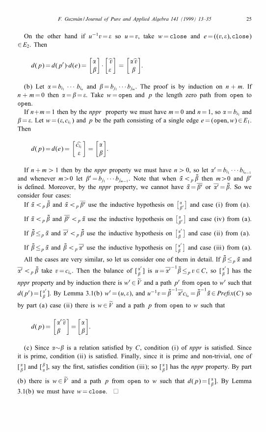
(c) Since �∼� is a relation satis�ed by C, condition (i) of nppr is satis�ed. Sinceit is prime, condition (ii) is satis�ed. Finally, since it is prime and non-trivial, one of

[��] and [�

�], say the �rst, satis�es condition (iii); so [�

�] has the nppr property. By part

(b) there is w∈ V and a path p from open to w such that d(p)= [��]. By Lemma

3.1(b) we must have w= close.


If we treat G, the simpli�ed domino group of C, as an automaton, with initial stateopen and �nal state close, by Lemma 3.1(c) L(G), the language accepted by G,

consists of dominoes [��] with the property that �∼ � is a relation satis�ed by C, and

therefore �≈� is an identity in M(C). If we use the domino to denote both the relationand the identity, depending on the context, we get the following theorem.

Theorem 3.3. Let C be a code; and G the simpli�ed domino graph of C: Then L(G)is a basis for the variety M(C).

Proof. Follows from Lemmas 1.4, 2.6, 3.1(c) and 3.2(c).

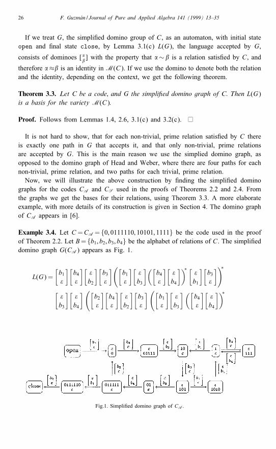
It is not hard to show, that for each non-trivial, prime relation satis�ed by C thereis exactly one path in G that accepts it, and that only non-trivial, prime relationsare accepted by G. This is the main reason we use the simplied domino graph, asopposed to the domino graph of Head and Weber, where there are four paths for eachnon-trivial, prime relation, and two paths for each trivial, prime relation.Now, we will illustrate the above construction by �nding the simpli�ed domino

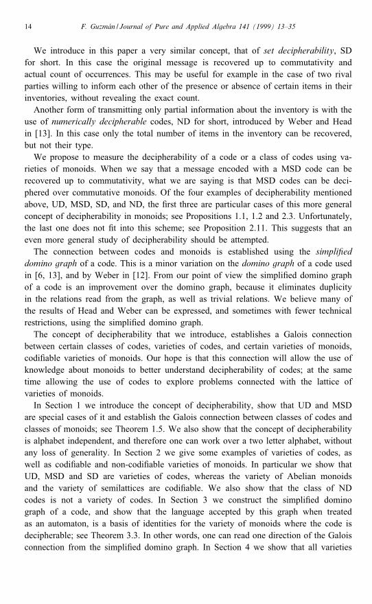
graphs for the codes CA and CS used in the proofs of Theorems 2.2 and 2.4. Fromthe graphs we get the bases for their relations, using Theorem 3.3. A more elaborateexample, with more details of its construction is given in Section 4. The domino graphof CA appears in [6].

Example 3.4. Let C =CA= {0; 0111110; 10101; 1111} be the code used in the proofof Theorem 2.2. Let B= {b1; b2; b3; b4} be the alphabet of relations of C. The simpli�eddomino graph G(CA) appears as Fig. 1.

L(G) =[b1�

][b4�

][�b2

][b3�

]([b1�

][�b3

]([b4�

][�b4

])∗ [�b1

][b3�

])∗[�b3

][�b4

]([b2�

][b4�

][�b2

][b3�

]([b1�

][�b3

]([b4�

][�b4

])∗

Fig.1. Simpli�ed domino graph of CA.


[�b1

] [b3�

])∗ [�b3

] [�b4

])∗ [�b1

] [b2�

]

=[b1�

]([b4�

][�b2

][b3�

]([b1�

][�b3

]([b4�

][�b4

])∗ [�b1

][b3�

])∗[�b3

][�b4

] [b2�

])+ [�b1

]

=

[b1(b4b3b2

(b1b3

(b4b4

)∗b3b1

)∗b2b3b4

)+b1

]:

Clearly all the identities in L(G) are consequences of commutativity. Therefore, byProposition 1.2, C is a MSD code.

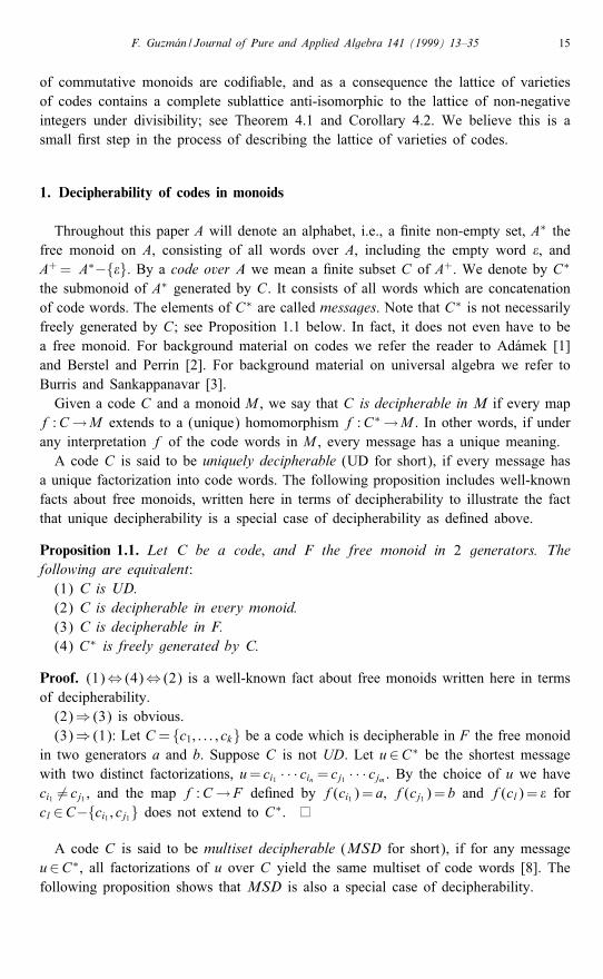
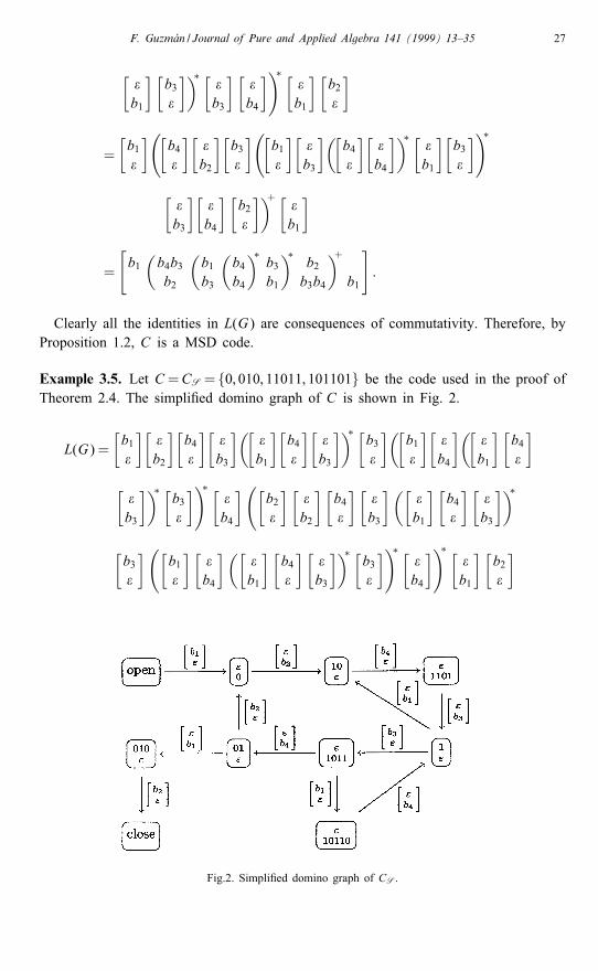
Example 3.5. Let C =CS= {0; 010; 11011; 101101} be the code used in the proof ofTheorem 2.4. The simpli�ed domino graph of C is shown in Fig. 2.

L(G) =[b1�

][�b2

][b4�

][�b3

]([�b1

][b4�

][�b3

])∗ [b3�

]([b1�

][�b4

]([�b1

] [b4�

][�b3

])∗ [b3�

])∗ [�b4

]([b2�

] [�b2

] [b4�

] [�b3

]([�b1

] [b4�

] [�b3

])∗[b3�

]([b1�

] [�b4

]([�b1

] [b4�

] [�b3

])∗ [b3�

])∗ [�b4

])∗ [�b1

] [b2�

]

Fig.2. Simpli�ed domino graph of CS.


=[b1�

]([�b2

][b4�

][�b3

]([�b1

][b4�

][�b3

])∗ [b3�

]([b1�

][�b4

]([�b1

][b4�

][�b3

])∗ [b3�

])∗ [�b4

] [b2�

])+ [�b1

]

=

b1 ( b4b2b3

(b4b1b3

)∗b3(b1b4

(b4b1b3

)∗b3)∗b2b4

)+b1

:This shows that C is SD (completing the proof of Theorem 2.4) since any non-trivial

relation [ ��] must include all four code words both on top and bottom. On the other

hand [ b1b4b4b3b2b2b3b1b3b4b1

]∈L(G). This shows that C is not MSD, verifying directly that the

inclusion MSD⊂ SD is strict (see Corollary 2.5).

4. Varieties of commutative monoids

In Section 2 we showed that the varieties of monoids, T, S, and A, are codi�able.In this section we show that this is also the case for all varieties of commutativemonoids.The varieties of commutative monoids were classi�ed by Head in [5]. It is shown

there that each proper variety of commutative monoids is determined by one identity inaddition to commutativity, namely xi= xi+p with i≥ 0; p≥ 1. Let’s denote this varietyby A(i; p). For example S=A(1; 1) and T=A(0; 1).

Theorem 4.1. Every variety V of commutative monoids is codi�able.

Proof. The case V =A is Theorem 2.2. The case V =A(i; p) with i¿0 will be treatedin detail, whereas the case V =A(0; p) will only be sketched; the details are similarto and simpler than those of i¿0.Let V =A(i; p) with i¿0, p≥ 1. Consider the code C =CA(i;p) = {c1; : : : ; c7} wherec1 = 001;

c2 = 100;

c3 = 01cp−11 0cp−12 10=0cp−12 101cp−11 0;

c4 = 11011011;

c5 = 11011;

c6 = 1110111;

c7 = 01(c2c6c1c5)i−1c2110=011(c1c5c2c6)i−1c110:


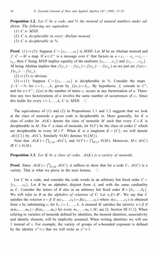
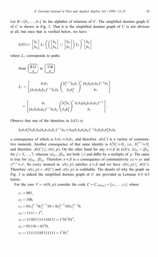
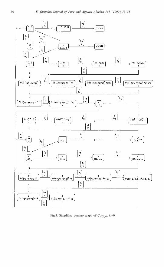
Let B={b1; : : : ; b7} be the alphabet of relations of C. The simpli�ed domino graph Gof C is shown in Fig. 3. That it is the simpli�ed domino graph of C is not obviousat all, but once that is veri�ed below, we have

L(G)=[b5b4

]L1

(([b4b4

]∪[b5b5

])L1

)∗ [b4b5

]where L1 corresponds to paths

from to

L1 =

[b7b1

(b1b5b2b6)i−1b1b2

(bp−11 b3b1b3b

p2

)∗(b2b6b1b5)i−1b2

b7

]

=

[b7

(b1b5b2b6)i−1b1b2

(bp1 b3b3b

p2

)∗b1b2(b6b1b5b2)i−1

b7

]:

Observe that one of the identities in L(G) is

b5b7bp1 b3b1b2(b6b1b5b2)

i−1b4≈ b4(b1b5b2b6)i−1b1b2b3bp2 b7b5

a consequence of which is b7b3≈ b3b7, and therefore M(C) is a variety of commuta-tive monoids. Another consequence of that same identity is bp1 b

i1≈ bi1, i.e., bp+i1 ≈ bi1

and therefore M(C)⊆A(i; p). On the other hand for any �≈ � in L(G), |�|bj = |�|bjfor j=3; : : : ; 7, whereas |�|b1 , |�|b1 are both ≥ i and di�er by a multiple of p. The sameis true for |�|b2 , |�|b2 . Therefore �≈ � is a consequence of commutativity xy≈yx andxp+i≈ xi. So every monoid in A(i; p) satis�es �≈ � and we have A(i; p)⊆M(C).Therefore A(i; p)=M(C) and A(i; p) is codi�able. The details of why the graph onFig. 3 is indeed the simpli�ed domino graph of C are provided in Lemmas 4.3–4.5below.For the case V =A(0; p) consider the code C =CA(0;p) = {c1; : : : ; c7} where

c1 = 001;

c2 = 100;

c3 = 01cp−11 0cp−12 10=0cp−12 101cp−11 0;

c4 = 1111=14;

c5 = 111011111110111=13017013;

c6 = 01110=0130;

c7 = 111111101111111=17017:


Fig.3. Simpli�ed domino graph of CA(i;p), i¿0.


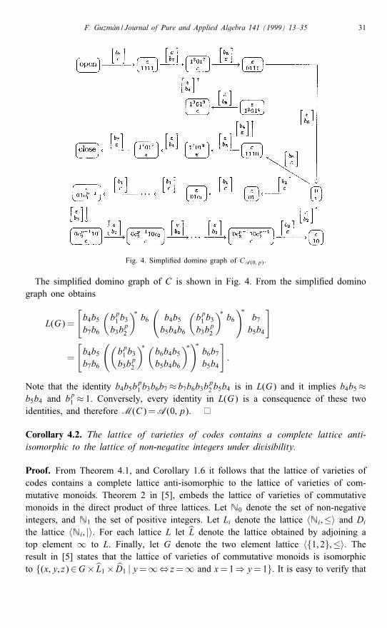
Fig. 4. Simpli�ed domino graph of CA(0; p).

The simpli�ed domino graph of C is shown in Fig. 4. From the simpli�ed dominograph one obtains

L(G) =

[b4b5b7b6

(bp1 b3b3b

p2

)∗b6(b4b5b5b4b6

(bp1 b3b3b

p2

)∗b6)∗

b7b5b4

]

=

[b4b5b7b6

((bp1 b3b3b

p2

)∗(b6b4b5b5b4b6

)∗)∗b6b7b5b4

]:

Note that the identity b4b5bp1 b3b6b7≈ b7b6b3bp2 b5b4 is in L(G) and it implies b4b5≈

b5b4 and bp1 ≈ 1. Conversely, every identity in L(G) is a consequence of these two

identities, and therefore M(C)=A(0; p).

Corollary 4.2. The lattice of varieties of codes contains a complete lattice anti-isomorphic to the lattice of non-negative integers under divisibility.

Proof. From Theorem 4.1, and Corollary 1.6 it follows that the lattice of varieties ofcodes contains a complete lattice anti-isomorphic to the lattice of varieties of com-mutative monoids. Theorem 2 in [5], embeds the lattice of varieties of commutativemonoids in the direct product of three lattices. Let N0 denote the set of non-negativeintegers, and N1 the set of positive integers. Let Li denote the lattice 〈Ni ;≤〉 and Dithe lattice 〈Ni ; |〉. For each lattice L let L denote the lattice obtained by adjoining atop element ∞ to L. Finally, let G denote the two element lattice 〈{1; 2};≤〉. Theresult in [5] states that the lattice of varieties of commutative monoids is isomorphicto {(x; y; z)∈G× L1× D1 |y=∞⇔ z=∞ and x=1⇒y=1}. It is easy to verify that


this lattice is isomorphic to [L0×D1 by mapping (1; 1; p) 7→ (0; p); (2; i; p) 7→ (i; p) and(2;∞;∞) 7→∞. Let Q= {q1; q2; : : :} be the set of all primes. Note that D1 is isomor-phic to the sublattice of

∏Q L0 consisting of sequences with �nite support, via the map

�(n)= (�1; �2; : : : ; �k ; 0; 0; : : :) where n= q�11 q

�22 · · · q�kk . So L0×D1 is isomorphic to D1

by mapping (i; n) 7→ (i; �1; �2; : : : ; �k ; 0; 0; : : :). Finally D1 is isomorphic to D0 since 0 isthe largest element of D0.

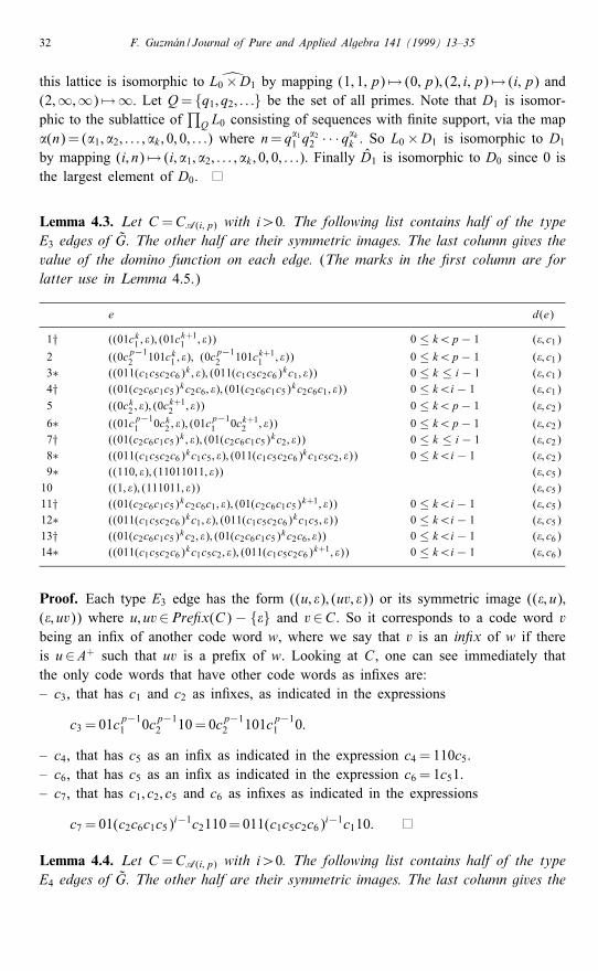
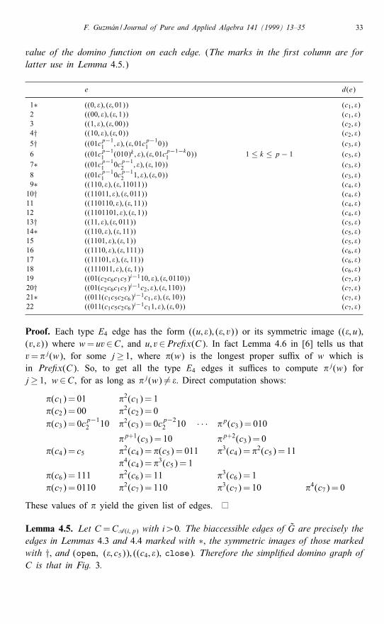
Lemma 4.3. Let C =CA(i; p) with i¿0. The following list contains half of the typeE3 edges of G. The other half are their symmetric images. The last column gives thevalue of the domino function on each edge. (The marks in the �rst column are forlatter use in Lemma 4.5.)

e d(e)

1† ((01ck1 ; �); (01ck+11 ; �)) 0 ≤ k¡p− 1 (�; c1)

2 ((0cp−12 101ck1 ; �); (0cp−12 101ck+11 ; �)) 0 ≤ k¡p− 1 (�; c1)

3∗ ((011(c1c5c2c6)k ; �); (011(c1c5c2c6)k c1; �)) 0 ≤ k ≤ i − 1 (�; c1)4† ((01(c2c6c1c5)k c2c6; �); (01(c2c6c1c5)k c2c6c1; �)) 0 ≤ k¡i − 1 (�; c1)5 ((0ck2 ; �); (0c

k+12 ; �)) 0 ≤ k¡p− 1 (�; c2)

6∗ ((01cp−11 0ck2 ; �); (01cp−11 0ck+12 ; �)) 0 ≤ k¡p− 1 (�; c2)

7† ((01(c2c6c1c5)k ; �); (01(c2c6c1c5)k c2; �)) 0 ≤ k ≤ i − 1 (�; c2)8∗ ((011(c1c5c2c6)k c1c5; �); (011(c1c5c2c6)k c1c5c2; �)) 0 ≤ k¡i − 1 (�; c2)9∗ ((110; �); (11011011; �)) (�; c5)10 ((1; �); (111011; �)) (�; c5)11† ((01(c2c6c1c5)k c2c6c1; �); (01(c2c6c1c5)k+1; �)) 0 ≤ k¡i − 1 (�; c5)12∗ ((011(c1c5c2c6)k c1; �); (011(c1c5c2c6)k c1c5; �)) 0 ≤ k¡i − 1 (�; c5)13† ((01(c2c6c1c5)k c2; �); (01(c2c6c1c5)k c2c6; �)) 0 ≤ k¡i − 1 (�; c6)14∗ ((011(c1c5c2c6)k c1c5c2; �); (011(c1c5c2c6)k+1; �)) 0 ≤ k¡i − 1 (�; c6)

Proof. Each type E3 edge has the form ((u; �); (uv; �)) or its symmetric image ((�; u);(�; uv)) where u; uv∈Pre�x(C) − {�} and v∈C. So it corresponds to a code word vbeing an in�x of another code word w, where we say that v is an in�x of w if thereis u∈A+ such that uv is a pre�x of w. Looking at C, one can see immediately thatthe only code words that have other code words as in�xes are:– c3, that has c1 and c2 as in�xes, as indicated in the expressions

c3 = 01cp−11 0cp−12 10=0cp−12 101cp−11 0:

– c4, that has c5 as an in�x as indicated in the expression c4 = 110c5.– c6, that has c5 as an in�x as indicated in the expression c6 = 1c51.– c7, that has c1; c2; c5 and c6 as in�xes as indicated in the expressions

c7 = 01(c2c6c1c5)i−1c2110=011(c1c5c2c6)i−1c110:

Lemma 4.4. Let C =CA(i; p) with i¿0. The following list contains half of the typeE4 edges of G. The other half are their symmetric images. The last column gives the


value of the domino function on each edge. (The marks in the �rst column are forlatter use in Lemma 4.5.)

e d(e)

1∗ ((0; �); (�; 01)) (c1; �)2 ((00; �); (�; 1)) (c1; �)3 ((1; �); (�; 00)) (c2; �)4† ((10; �); (�; 0)) (c2; �)5† ((01cp−11 ; �); (�; 01cp−11 0)) (c3; �)6 ((01cp−11 (010)k ; �); (�; 01cp−1−k1 0)) 1 ≤ k ≤ p− 1 (c3; �)7∗ ((01cp−11 0cp−12 ; �); (�; 10)) (c3; �)8 ((01cp−11 0cp−12 1; �); (�; 0)) (c3; �)9∗ ((110; �); (�; 11011)) (c4; �)10† ((11011; �); (�; 011)) (c4; �)11 ((110110; �); (�; 11)) (c4; �)12 ((1101101; �); (�; 1)) (c4; �)13† ((11; �); (�; 011)) (c5; �)14∗ ((110; �); (�; 11)) (c5; �)15 ((1101; �); (�; 1)) (c5; �)16 ((1110; �); (�; 111)) (c6; �)17 ((11101; �); (�; 11)) (c6; �)18 ((111011; �); (�; 1)) (c6; �)19 ((01(c2c6c1c5)i−110; �); (�; 0110)) (c7; �)20† ((01(c2c6c1c5)i−1c2; �); (�; 110)) (c7; �)21∗ ((011(c1c5c2c6)i−1c1; �); (�; 10)) (c7; �)22 ((011(c1c5c2c6)i−1c11; �); (�; 0)) (c7; �)

Proof. Each type E4 edge has the form ((u; �); (�; v)) or its symmetric image ((�; u);(v; �)) where w= uv∈C, and u; v∈Pre�x(C). In fact Lemma 4.6 in [6] tells us thatv= �j(w), for some j≥ 1, where �(w) is the longest proper su�x of w which isin Pre�x(C). So, to get all the type E4 edges it su�ces to compute �j(w) forj≥ 1; w∈C, for as long as �j(w) 6= �. Direct computation shows:

�(c1)= 01 �2(c1)= 1�(c2)= 00 �2(c2)= 0�(c3)= 0c

p−12 10 �2(c3)= 0c

p−22 10 · · · �p(c3)= 010

�p+1(c3)= 10 �p+2(c3)= 0�(c4)= c5 �2(c4)= �(c5)= 011 �3(c4)= �2(c5)= 11

�4(c4)= �3(c5)= 1�(c6)= 111 �2(c6)= 11 �3(c6)= 1�(c7)= 0110 �2(c7)= 110 �3(c7)= 10 �4(c7)= 0

These values of � yield the given list of edges.

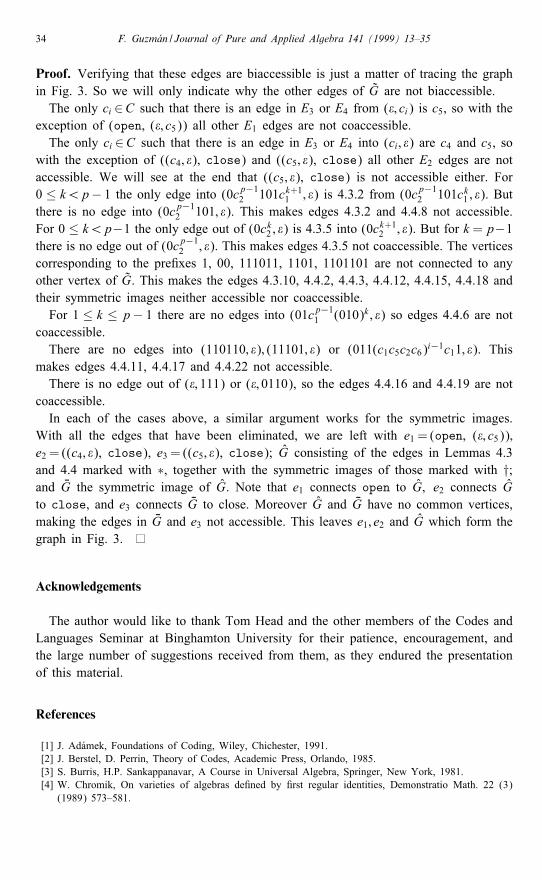
Lemma 4.5. Let C =CA(i; p) with i¿0. The biaccessible edges of G are precisely theedges in Lemmas 4.3 and 4.4 marked with ∗; the symmetric images of those markedwith †; and (open; (�; c5)); ((c4; �); close). Therefore the simpli�ed domino graph ofC is that in Fig. 3.


Proof. Verifying that these edges are biaccessible is just a matter of tracing the graphin Fig. 3. So we will only indicate why the other edges of G are not biaccessible.The only ci ∈C such that there is an edge in E3 or E4 from (�; ci) is c5, so with the

exception of (open, (�; c5)) all other E1 edges are not coaccessible.The only ci ∈C such that there is an edge in E3 or E4 into (ci; �) are c4 and c5, so

with the exception of ((c4; �), close) and ((c5; �), close) all other E2 edges are notaccessible. We will see at the end that ((c5; �), close) is not accessible either. For0 ≤ k¡p− 1 the only edge into (0cp−12 101ck+11 ; �) is 4.3.2 from (0cp−12 101ck1 ; �). Butthere is no edge into (0cp−12 101; �). This makes edges 4.3.2 and 4.4.8 not accessible.For 0 ≤ k¡p−1 the only edge out of (0ck2 ; �) is 4.3.5 into (0ck+12 ; �). But for k =p−1there is no edge out of (0cp−12 ; �). This makes edges 4.3.5 not coaccessible. The verticescorresponding to the pre�xes 1, 00, 111011, 1101, 1101101 are not connected to anyother vertex of G. This makes the edges 4.3.10, 4.4.2, 4.4.3, 4.4.12, 4.4.15, 4.4.18 andtheir symmetric images neither accessible nor coaccessible.For 1 ≤ k ≤ p− 1 there are no edges into (01cp−11 (010)k ; �) so edges 4.4.6 are not

coaccessible.There are no edges into (110110; �); (11101; �) or (011(c1c5c2c6)i−1c11; �). This

makes edges 4.4.11, 4.4.17 and 4.4.22 not accessible.There is no edge out of (�; 111) or (�; 0110), so the edges 4.4.16 and 4.4.19 are not

coaccessible.In each of the cases above, a similar argument works for the symmetric images.

With all the edges that have been eliminated, we are left with e1 = (open, (�; c5));e2 = ((c4; �), close), e3 = ((c5; �), close); G consisting of the edges in Lemmas 4.3and 4.4 marked with ∗, together with the symmetric images of those marked with †;and �G the symmetric image of G. Note that e1 connects open to G; e2 connects Gto close, and e3 connects �G to close. Moreover G and �G have no common vertices,making the edges in �G and e3 not accessible. This leaves e1; e2 and G which form thegraph in Fig. 3.

Acknowledgements

The author would like to thank Tom Head and the other members of the Codes andLanguages Seminar at Binghamton University for their patience, encouragement, andthe large number of suggestions received from them, as they endured the presentationof this material.

References

[1] J. Ad�amek, Foundations of Coding, Wiley, Chichester, 1991.[2] J. Berstel, D. Perrin, Theory of Codes, Academic Press, Orlando, 1985.[3] S. Burris, H.P. Sankappanavar, A Course in Universal Algebra, Springer, New York, 1981.[4] W. Chromik, On varieties of algebras de�ned by �rst regular identities, Demonstratio Math. 22 (3)

(1989) 573–581.


[5] T.J. Head, The varieties of commutative monoids, Nieuw Arch. Wisk. 16 (3) (1968) 203–206.[6] T.J. Head, A. Weber, Deciding multiset decipherability, IEEE Trans. Inform. Theory 41 (1) (1995)

291–297.[7] B. J�onsson, E. Nelson, Relatively free products in regular varieties, Algebra Universalis 4 (1974)

14–19.[8] A. Lempel, On multiset decipherable codes, IEEE Trans. Inform. Theory 32 (5) (1986) 714–716.[9] O. Ore, Galois connexions, Trans. Amer. Math. Soc. 55 (1944) 493–513.[10] J. Plonka, On a method of construction of abstract algebras, Fund. Math. 61 (1967) 183–189.[11] A. Restivo, A note on multiset decipherable codes, IEEE Trans. Inform. Theory 35 (3) (1989)

662–663.[12] A. Weber, Computing the intercode index by means of dominoes, preprint.[13] A. Weber, T.J. Head, The �nest homophonic partition and related code concepts, in: I. Pr��vara,

B. Rovan, P. Ru�zi�cka (Eds.), Mathematical Foundations of Computer Science 1994, Lecture Notesin Computer Science, vol. 841, Springer, Berlin, 1994, pp. 618–628.

Documents

Decipherability of codes