Analysing Quantitative Data

AnAlysing

QuAntitAtive DAtA

00_Kent_Prelims.indd 1 25/02/2015 11:15:35 AM

2DATA PREPARATION

Learning objectives

In this chapter you will learn:

•• how datasets are prepared, ready for the next stages of data analysis;•• that all data need to be checked, edited, coded and assembled before any

further processes can take place;•• that the transformation of some of the properties in a dataset may involve

one or more of a number of activities, including, for variables, regrouping values on a nominal or ordered category measure to create fewer categories, creating class intervals from metric measures, computing totals or other scores from combinations of several variables, treating groups of variables as a multiple response question, upgrading or downgrading measures, han-dling missing values and ‘Don’t know’ responses, or coding open-ended questions;

•• that, for set memberships, transformations may entail creating crisp sets or fuzzy sets from existing variables;

•• how survey analysis software like SPSS can be used for assembling data and assisting in data transformations;

•• that many of the codes used in the original alcohol marketing dataset were illogical or inconsistent and many data transformations were needed before analysis could begin.

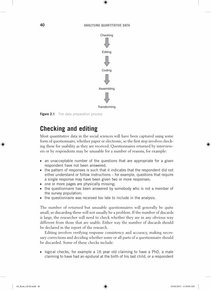
IntroductionBefore quantitative data that have been constructed by researchers can be ana-lysed using techniques appropriate for pursuing the objectives of the research, they need to be prepared in various ways to make them ready for analysis. In their raw form, captured data will consist of stacks of completed paper question-naires or diaries, entries into an online questionnaire or records made by researchers themselves. Before statistical techniques can be applied to the data, they will need to undergo many of the various processes listed in Figure 2.1.

02_Kent_Ch 02.indd 39 25/02/2015 11:59:05 AM

ANALYSING QUANTITATIVE DATA40

Checking and editingMost quantitative data in the social sciences will have been captured using some form of questionnaire, whether paper or electronic, so the first step involves check-ing these for usability as they are received. Questionnaires returned by interview-ers or by respondents may be unusable for a number of reasons, for example:

•• an unacceptable number of the questions that are appropriate for a given respondent have not been answered;

•• the pattern of responses is such that it indicates that the respondent did not either understand or follow instructions – for example, questions that require a single response may have been given two or more responses;

•• one or more pages are physically missing;•• the questionnaire has been answered by somebody who is not a member of

the survey population;•• the questionnaire was received too late to include in the analysis.

The number of returned but unusable questionnaires will generally be quite small, so discarding these will not usually be a problem. If the number of discards is large, the researcher will need to check whether they are in any obvious way different from those that are usable. Either way the number of discards should be declared in the report of the research.

Editing involves verifying response consistency and accuracy, making neces-sary corrections and deciding whether some or all parts of a questionnaire should be discarded. Some of these checks include:

•• logical checks, for example a 16 year old claiming to have a PhD, a male claiming to have had an epidural at the birth of his last child, or a respondent

Figure 2.1 The data preparation process

Checking

Editing

Coding

Assembling

Transforming

02_Kent_Ch 02.indd 40 25/02/2015 11:59:05 AM

DATA PREPARATION 41

may have answered a series of questions about his or her usage of a partic-ular product, but other responses indicate that he or she does not possess one or has never used one;

•• range checks, for example a code of 8 is entered when there are only six response categories for that question;

•• response set checks, for example somebody has ‘strongly agreed’ with all the items on a Likert scale.

Where a question fails a logical check, then the pattern of responses in the rest of the questionnaire may be scrutinized to see what is the most likely explanation for the apparent inconsistency. Range check failures may be referred back to the original respondent. Response set checks may indicate that the respondent is simply being frivolous and the questionnaire may be discarded.

If questionnaires are checked and edited as they come in, it may still be possible to remedy fieldwork deficiencies before they turn into a major problem. If prob-lems are traced to particular interviewers, for example, then they can be replaced or asked to undergo further training. It may be possible to re-contact respondents to seek clarification or completion before the last date on which data can be pro-cessed. If this is not feasible, the researcher can treat these as missing values, that is, treat the questions involved as unanswered. This may be suitable if the unsatis-factory responses are not key properties and the number of questions concerned is quite small. If this is not the case, values may be imputed. How this can be done is discussed later in the chapter. The alternative is to discard the questionnaire.

CodingAs was explained in Chapter 1, data analysis software usually requires that all the values to be entered are either already numerical (as in age = 23) or they are given a number that is a code that ‘stands for’ values that are in words. Binary variables will normally be coded either as 1 or 0 or as 1 or 2. The categories for nominal and ordered category variables will generally be numbered 1, 2, 3, 4, and so on. Note that it makes sense for ordered categories to give the highest code number to the highest or most positive value as in Figures 1.2 and 1.3 in Chapter 1. Metric data already have numerical values that can be entered directly, for example the number of units of alcohol consumed last week as 10.7. Some, perhaps all, of the categorical responses on a questionnaire will have been pre-coded, that is they are already numbered on the questionnaire. If not, they need to be coded afterwards by the researcher.

Qualitative responses to open-ended questions will normally be classified into categories, which are then coded. The categories developed should meet the minimum requirements for a binary or nominal measure, namely, they should be exhaustive, mutually exclusive and refer to a single dimension. If, however, most of the spaces left for text in the questionnaire have been left empty, it may not be worthwhile doing this. Some pre-coded questions may have an ‘Other, please specify’ category, in which case some further coding may be worthwhile.

02_Kent_Ch 02.indd 41 25/02/2015 11:59:05 AM


If a question is unanswered, the researcher, when entering data into a survey analysis program, can record a missing value or enter a code for, for example, ‘Not applicable’ or ‘Refused to answer’. For multiple response questions where the respondent can indicate more than one category as applicable, each response category will need to be treated as a separate variable, and will usually be coded as 1 if the category is ticked and 0 or 2 if not. The treatment of open-ended and multiple response questions is considered in more detail later in this chapter.

In large-scale projects, and particularly when data entry is to be performed by a number of people or by subcontractors, researchers will often develop a code-book, which lists all the variable names (which are short, one-word identifiers), the variable labels (which are more extended descriptions of the variables and which appear as table or chart headings), the response categories used and the code numbers assigned. This means that any researcher can work on the dataset irrespective of whether or not they were involved in the project in its formative stages. Codebooks, however, are not always needed. Survey analysis packages like SPSS record all this information as part of the data matrix.

AssemblingData assembly means gathering together all the checked, edited and coded questionnaires, diaries or other forms of record, and entering the values for each variable for each case into data analysis software. This is usually achieved in a framework of rows and columns for storing the data called a data matrix. Data matrices are explained in more detail in Chapter 3. The range of software for assembling data is briefly reviewed at the end of Chapter 4. Some research-ers like to assemble data first into a spreadsheet like Excel before exporting to a survey analysis package. Some survey analysis software packages allow the researcher to enter the data by clicking the appropriate box against the answer given on an electronic version of the questionnaire. In the background, the software creates the data matrix. The researcher does not need to pre-code response categories in the questionnaire nor engage in post-coding when the questionnaires have been completed. With online surveys, the data matrix is automatically built up as respondents submit their completed online question-naires. Box 2.1 explains how to enter data into SPSS, the package that will be used throughout this text.

Mistakes can, of course, occur in the data entry process. Any entry that is outside the range of codes that have been allocated to a given variable will quickly show up in a table. Provided the questionnaires have been numbered, it is a simple matter to check the number of the respondent from the data matrix where the wrong codes have been entered and find what the code should have been from the questionnaire. In some packages any entry that is outside of a specified range will be flagged as the data are being keyed in. To detect erroneous codes that are inside the specified range, data may be subjected to double-entry data validation. In effect this means that the data are entered twice, usually by

02_Kent_Ch 02.indd 42 25/02/2015 11:59:05 AM

DATA PREPARATION 43

two different people, and any discrepancies in the two entries are flagged up by the computer and can be checked against the original questionnaire.

Box 2.1 Entering data into IBM SPSS Statistics

This software is one of the most widely used survey analysis computer programs and focuses exclusively on variable-based statistical analysis. It has gone through many versions, the latest being version 22.0. This text uses version 19.0. For more infor-mation and a free download of a demo version visit www.spss.com/spss.

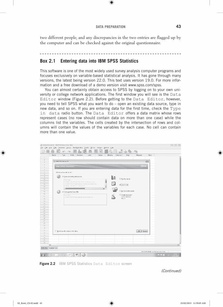
You can almost certainly obtain access to SPSS by logging on to your own uni-versity or college network applications. The first window you will see is the Data Editor window (Figure 2.2). Before getting to the Data Editor, however, you need to tell SPSS what you want to do – open an existing data source, type in new data, and so on. If you are entering data for the first time, check the Type in data radio button. The Data Editor offers a data matrix whose rows represent cases (no row should contain data on more than one case) while the columns list the variables. The cells created by the intersection of rows and col-umns will contain the values of the variables for each case. No cell can contain more than one value.

Figure 2.2 IBM SPSS Statistics Data Editor screen

(Continued)

02_Kent_Ch 02.indd 43 25/02/2015 11:59:05 AM


The alcohol marketing dataset was introduced in Chapter 1. The full dataset consists of 61 properties and 920 cases, and is available at https://study.sagepub.com/kent. As an exercise in data entry, instead of attempting to enter over 40,000 values, try entering just the nine key variables for the first 12 cases that are illustrated in the next chapter in Figure 3.1.

The key dependent variables relate to alcohol drinking behaviour and included here are Drinkstatus (whether or not they had ever had a proper alcoholic drink), Intentions (whether they think they will drink alcohol at any time in the next year) and Initiation (how old they were when they had their first proper alcoholic drink). Three key independent variables have been picked out: Totalaware (the number of alcohol marketing channels seen), Totalinvolve (the number of marketing involvements) and Likeads (how they feel about alco-hol ads as a whole). Finally, there are two demographics: Gender (male or female) and Socialclass (A, B, C1, C2, D, E).

Before entering any data, it is advisable first to name the variables (if you do not, you will be supplied with exciting names like var00001 and var00002). These names must begin with a letter and must not end with a full stop/period. There must be no spaces and the names chosen should not be one of the key words that SPSS uses as special computing terms, for example and, not, eq, by, all.

To enter variable names, click on the Variable View tab at the bottom left of the Data Editor window. Each variable now occupies a row rather than a column as in the Data Editor window. Enter the name of the first variable Drinkstatus in the top left box. As soon as you hit Enter or the down arrow or right arrow, the remaining boxes will be filled with default settings, except for Label. It is always better to enter labels, since these are what are printed out in your tables and graphs. Labels can be the wording of the questions asked or a fur-ther explanation of the variable. For Drinkstatus, you can, for example, type in Have you ever had a proper alcohol drink? You can put in labels for the remaining seven variables.

For categorical variables, you will also need to put in Values and Value Labels. Click on the appropriate cell under Values and click again on the little blue box to the right of the cell. This will produce the Value Labels dialog box. Enter an appropriate code value (e.g. 1) and label Yes and click on Add. Repeat for each value. Note that, in SPSS, allocated codes are called ‘values’, while the values in words are ‘labels’.

The default under Decimals is usually two decimal places. If all the vari-ables are integers, then it is worthwhile changing this to 0. Simply click on the cell and use the little down arrow to reduce to zero. Under Measure, you can put in the correct type of measure – Nominal, Ordinal or Scale. Note that Nominal includes binary measures, Ordinal does not distinguish between ordered category and ranked measures, and Scale refers to what have been called metric measures in Chapter 1. The default setting is Scale. Changing Measure to Nominal or Ordinal as appropriate creates a useful icon against each listed variable, making them easy to spot; it makes a difference to some operations in SPSS and forces you to think about what kind of measure is attained by each variable.

(Continued)

02_Kent_Ch 02.indd 44 25/02/2015 11:59:05 AM

DATA PREPARATION 45

To copy any variable information to another variable, like value labels, just use Edit/Copy and Paste. SPSS does not have an automatic timed backup facil-ity. You need to save your work regularly as you go along. Use the File|Save sequence as usual for Windows applications. The first time you go to save, you will be given the Save As dialog box. Make sure this indicates the drive you want. File|Exit will get you out of SPSS and back to the Program Manager or Windows desktop. SPSS will ask you if you want to save before exiting if unsaved changes have been made. Always save any changes to your data, but saving output is less important because it can quickly be recreated. The completed Variable View is shown in Figure 2.3.

Key points and wider issues

The careful checking, editing, coding and assembly of data should never be neglected. If poor-quality data are entered into the analysis, then no matter how sophisticated the statistical techniques applied, a poor or untrustworthy analysis will result. In this context the phrase ‘Garbage In, Garbage Out’ (or GIGO) is often mentioned. Checking, editing, coding, assembly and entry of data into a data matrix will commonly account for a substantial amount of time that an analyst will spend on the data.

Figure 2.3 The completed Variable View

02_Kent_Ch 02.indd 45 25/02/2015 11:59:06 AM


TransformingBefore beginning data analysis, the researcher may wish to transform some of the variables in a number of ways that might include:

•• regrouping values on a nominal or ordered category measure to create fewer categories;

•• creating class intervals from metric measures;•• computing totals or other scores from combinations of several values of

variables;•• treating groups of variables as a single multiple response question;•• upgrading or downgrading measures;•• handling missing values and ‘Don’t know’ responses;•• coding open-ended questions;•• creating crisp or fuzzy set memberships from nominal, ordered category,

ranked or metric measures.

Most of these tasks can be accomplished by using SPSS procedures, which are explained in Boxes 2.2–2.6 in this chapter.

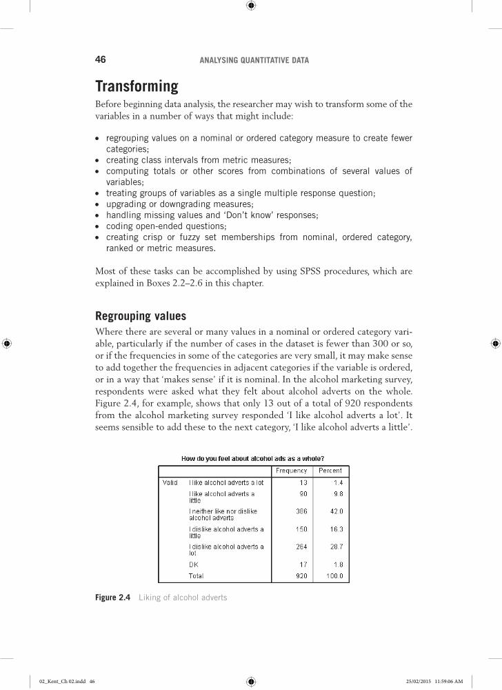
Regrouping valuesWhere there are several or many values in a nominal or ordered category vari-able, particularly if the number of cases in the dataset is fewer than 300 or so, or if the frequencies in some of the categories are very small, it may make sense to add together the frequencies in adjacent categories if the variable is ordered, or in a way that ‘makes sense’ if it is nominal. In the alcohol marketing survey, respondents were asked what they felt about alcohol adverts on the whole. Figure 2.4, for example, shows that only 13 out of a total of 920 respondents from the alcohol marketing survey responded ‘I like alcohol adverts a lot’. It seems sensible to add these to the next category, ‘I like alcohol adverts a little’.

Figure 2.4 Liking of alcohol adverts

02_Kent_Ch 02.indd 46 25/02/2015 11:59:06 AM

DATA PREPARATION 47

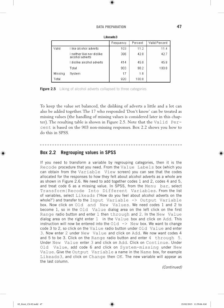
To keep the value set balanced, the disliking of adverts a little and a lot can also be added together. The 17 who responded ‘Don’t know’ can be treated as missing values (the handling of missing values is considered later in this chap-ter). The resulting table is shown in Figure 2.5. Note that the Valid Per-cent is based on the 903 non-missing responses. Box 2.2 shows you how to do this in SPSS.

Box 2.2 Regrouping values in SPSS

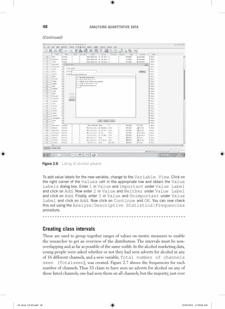
If you need to transform a variable by regrouping categories, then it is the Recode procedure that you need. From the Value Labels box (which you can obtain from the Variable View screen) you can see that the codes allocated for the responses to how they felt about alcohol adverts as a whole are as shown in Figure 2.6. We need to add together codes 1 and 2, codes 4 and 5, and treat code 6 as a missing value. In SPSS, from the Menu bar, select Transform|Recode Into Different Variables. From the list of variables, select Likeads (‘How do you feel about alcohol adverts on the whole?’) and transfer to the Input Variable -> Output Variable box. Now click on Old and New Values. We need codes 1 and 2 to become 1, so in the Old Value dialog area on the left click on the first Range radio button and enter 1 then through and 2. In the New Value dialog area on the right enter 1 in the Value box and click on Add. This instruction will now be entered into the Old -> New box. We want to change code 3 to 2, so click on the Value radio button under Old Value and enter 3. Now enter 2 under New Value and click on Add. We now want codes 4 and 5 to be 3. Click on the Range radio button and enter 4 through 5. Under New Value enter 3 and click on Add. Click on Continue. Under Old Value, add code 6 and click on System-missing under New Value. Give the Output Variable a name in the Name box, for example Likeads3, and click on Change then OK. The new variable will appear as the last column.

Figure 2.5 Liking of alcohol adverts collapsed to three categories

(Continued)

02_Kent_Ch 02.indd 47 25/02/2015 11:59:06 AM


To add value labels for the new variable, change to the Variable View. Click on the right corner of the Values cell in the appropriate row and obtain the Value Labels dialog box. Enter 1 in Value and Important under Value Label and click on Add. Now enter 2 in Value and Neither under Value Label and click on Add. Finally, enter 3 in Value and Unimportant under Value Label and click on Add. Now click on Continue and OK. You can now check this out using the Analyze|Descriptive Statistics|Frequencies procedure.

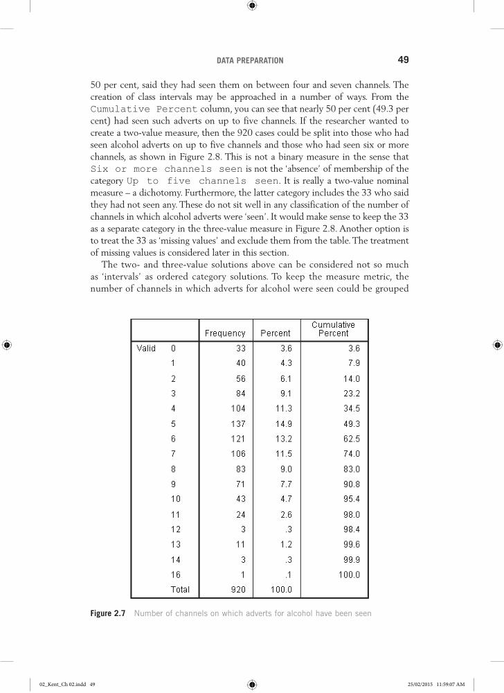
Creating class intervalsThese are used to group together ranges of values on metric measures to enable the researcher to get an overview of the distribution. The intervals must be non-overlapping and as far as possible of the same width. In the alcohol marketing data, young people were asked whether or not they had seen adverts for alcohol in any of 16 different channels, and a new variable, Total number of channels seen (Totalseen), was created. Figure 2.7 shows the frequencies for each number of channels. Thus 33 claim to have seen no adverts for alcohol on any of these listed channels, one had seen them on all channels, but the majority, just over

Figure 2.6 Liking of alcohol adverts

(Continued)

02_Kent_Ch 02.indd 48 25/02/2015 11:59:06 AM

DATA PREPARATION 49

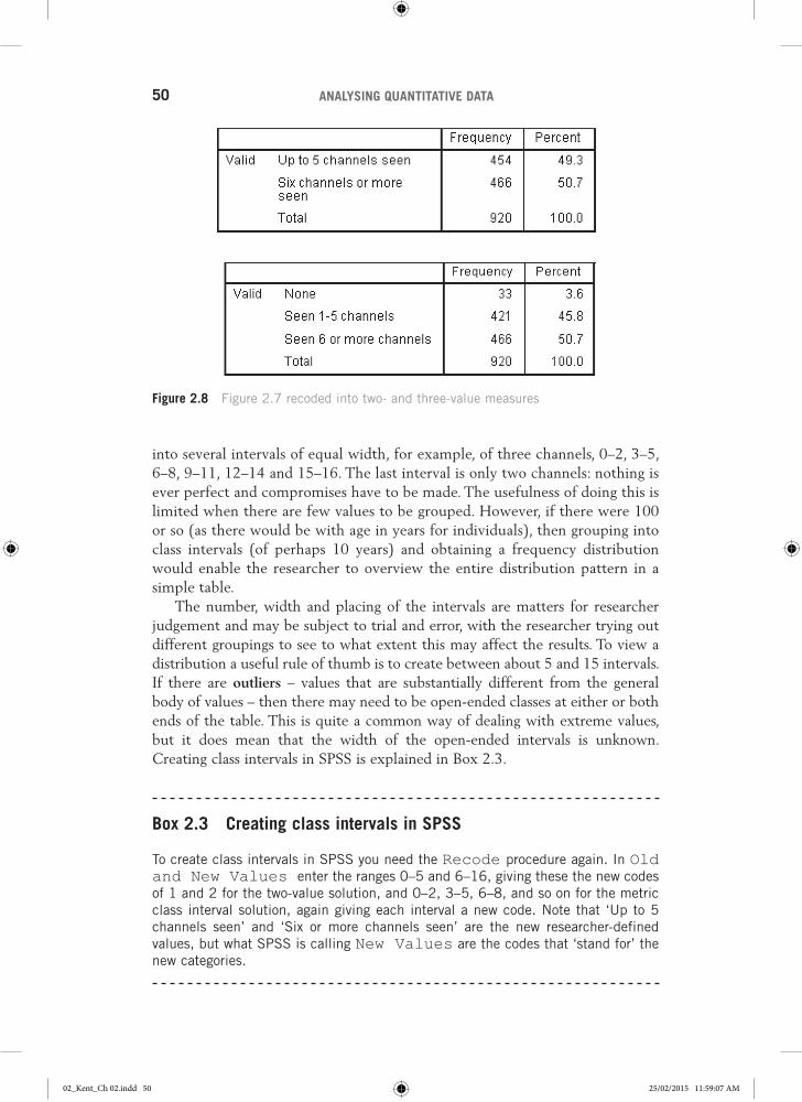
50 per cent, said they had seen them on between four and seven channels. The creation of class intervals may be approached in a number of ways. From the Cumulative Percent column, you can see that nearly 50 per cent (49.3 per cent) had seen such adverts on up to five channels. If the researcher wanted to create a two-value measure, then the 920 cases could be split into those who had seen alcohol adverts on up to five channels and those who had seen six or more channels, as shown in Figure 2.8. This is not a binary measure in the sense that Six or more channels seen is not the ‘absence’ of membership of the category Up to five channels seen. It is really a two-value nominal measure – a dichotomy. Furthermore, the latter category includes the 33 who said they had not seen any. These do not sit well in any classification of the number of channels in which alcohol adverts were ‘seen’. It would make sense to keep the 33 as a separate category in the three-value measure in Figure 2.8. Another option is to treat the 33 as ‘missing values’ and exclude them from the table. The treatment of missing values is considered later in this section.

The two- and three-value solutions above can be considered not so much as ‘intervals’ as ordered category solutions. To keep the measure metric, the number of channels in which adverts for alcohol were seen could be grouped

Figure 2.7 Number of channels on which adverts for alcohol have been seen

02_Kent_Ch 02.indd 49 25/02/2015 11:59:07 AM


Figure 2.8 Figure 2.7 recoded into two- and three-value measures

into several intervals of equal width, for example, of three channels, 0–2, 3–5, 6–8, 9–11, 12–14 and 15–16. The last interval is only two channels: nothing is ever perfect and compromises have to be made. The usefulness of doing this is limited when there are few values to be grouped. However, if there were 100 or so (as there would be with age in years for individuals), then grouping into class intervals (of perhaps 10 years) and obtaining a frequency distribution would enable the researcher to overview the entire distribution pattern in a simple table.

The number, width and placing of the intervals are matters for researcher judgement and may be subject to trial and error, with the researcher trying out different groupings to see to what extent this may affect the results. To view a distribution a useful rule of thumb is to create between about 5 and 15 intervals. If there are outliers – values that are substantially different from the general body of values – then there may need to be open-ended classes at either or both ends of the table. This is quite a common way of dealing with extreme values, but it does mean that the width of the open-ended intervals is unknown. Creating class intervals in SPSS is explained in Box 2.3.

Box 2.3 Creating class intervals in SPSS

To create class intervals in SPSS you need the Recode procedure again. In Old and New Values enter the ranges 0–5 and 6–16, giving these the new codes of 1 and 2 for the two-value solution, and 0–2, 3–5, 6–8, and so on for the metric class interval solution, again giving each interval a new code. Note that ‘Up to 5 channels seen’ and ‘Six or more channels seen’ are the new researcher-defined values, but what SPSS is calling New Values are the codes that ‘stand for’ the new categories.

02_Kent_Ch 02.indd 50 25/02/2015 11:59:07 AM

DATA PREPARATION 51

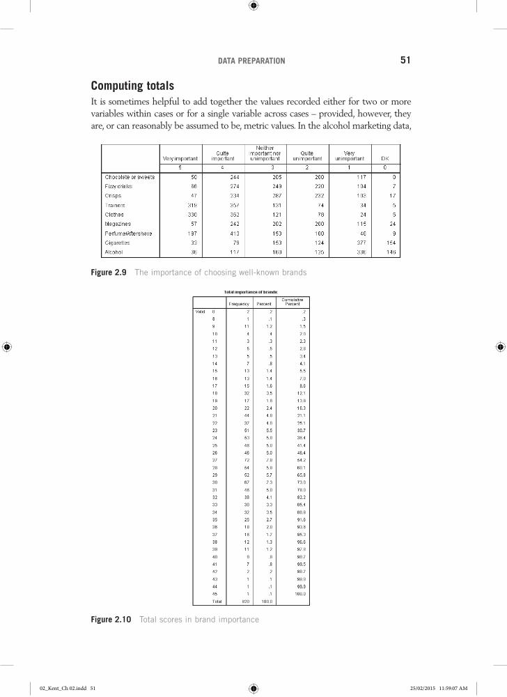
Computing totalsIt is sometimes helpful to add together the values recorded either for two or more variables within cases or for a single variable across cases – provided, however, they are, or can reasonably be assumed to be, metric values. In the alcohol marketing data,

Figure 2.9 The importance of choosing well-known brands

Figure 2.10 Total scores in brand importance

02_Kent_Ch 02.indd 51 25/02/2015 11:59:07 AM


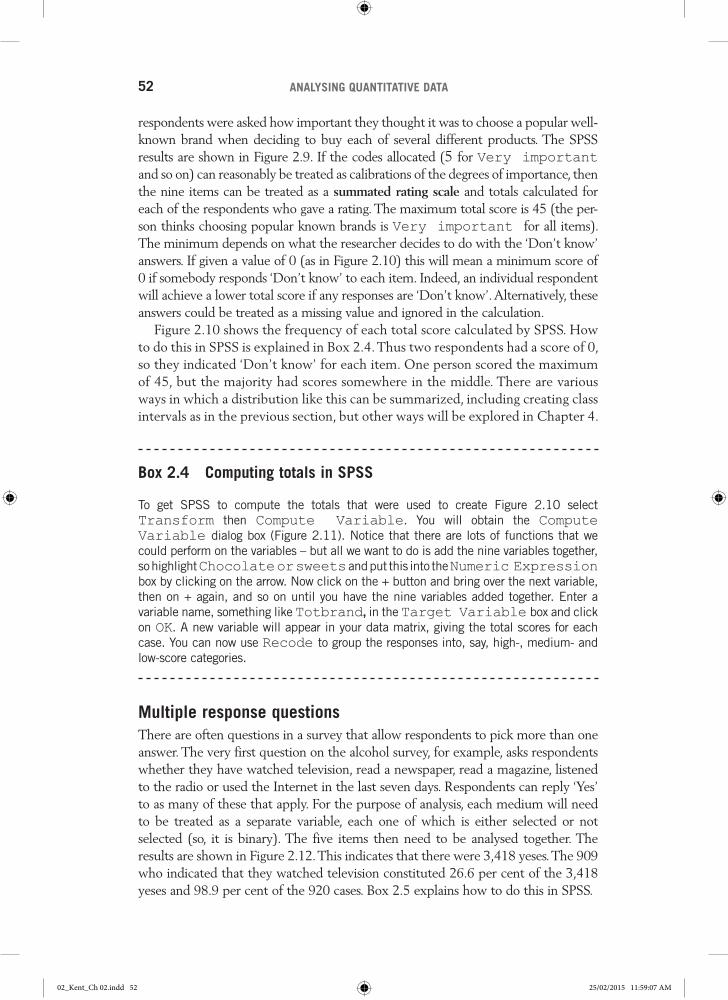
respondents were asked how important they thought it was to choose a popular well-known brand when deciding to buy each of several different products. The SPSS results are shown in Figure 2.9. If the codes allocated (5 for Very important and so on) can reasonably be treated as calibrations of the degrees of importance, then the nine items can be treated as a summated rating scale and totals calculated for each of the respondents who gave a rating. The maximum total score is 45 (the per-son thinks choosing popular known brands is Very important for all items). The minimum depends on what the researcher decides to do with the ‘Don’t know’ answers. If given a value of 0 (as in Figure 2.10) this will mean a minimum score of 0 if somebody responds ‘Don’t know’ to each item. Indeed, an individual respondent will achieve a lower total score if any responses are ‘Don’t know’. Alternatively, these answers could be treated as a missing value and ignored in the calculation.

Figure 2.10 shows the frequency of each total score calculated by SPSS. How to do this in SPSS is explained in Box 2.4. Thus two respondents had a score of 0, so they indicated ‘Don’t know’ for each item. One person scored the maximum of 45, but the majority had scores somewhere in the middle. There are various ways in which a distribution like this can be summarized, including creating class intervals as in the previous section, but other ways will be explored in Chapter 4.

Box 2.4 Computing totals in SPSS

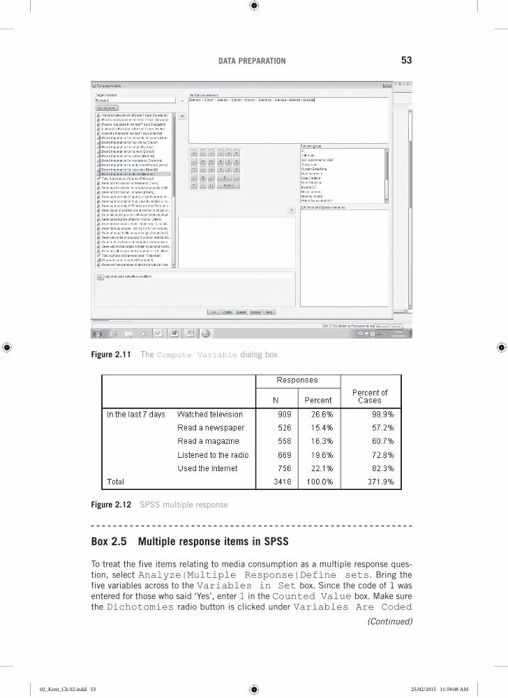
To get SPSS to compute the totals that were used to create Figure 2.10 select Transform then Compute Variable. You will obtain the Compute Variable dialog box (Figure 2.11). Notice that there are lots of functions that we could perform on the variables – but all we want to do is add the nine variables together, so highlight Chocolate or sweets and put this into the Numeric Expression box by clicking on the arrow. Now click on the + button and bring over the next variable, then on + again, and so on until you have the nine variables added together. Enter a variable name, something like Totbrand, in the Target Variable box and click on OK. A new variable will appear in your data matrix, giving the total scores for each case. You can now use Recode to group the responses into, say, high-, medium- and low-score categories.

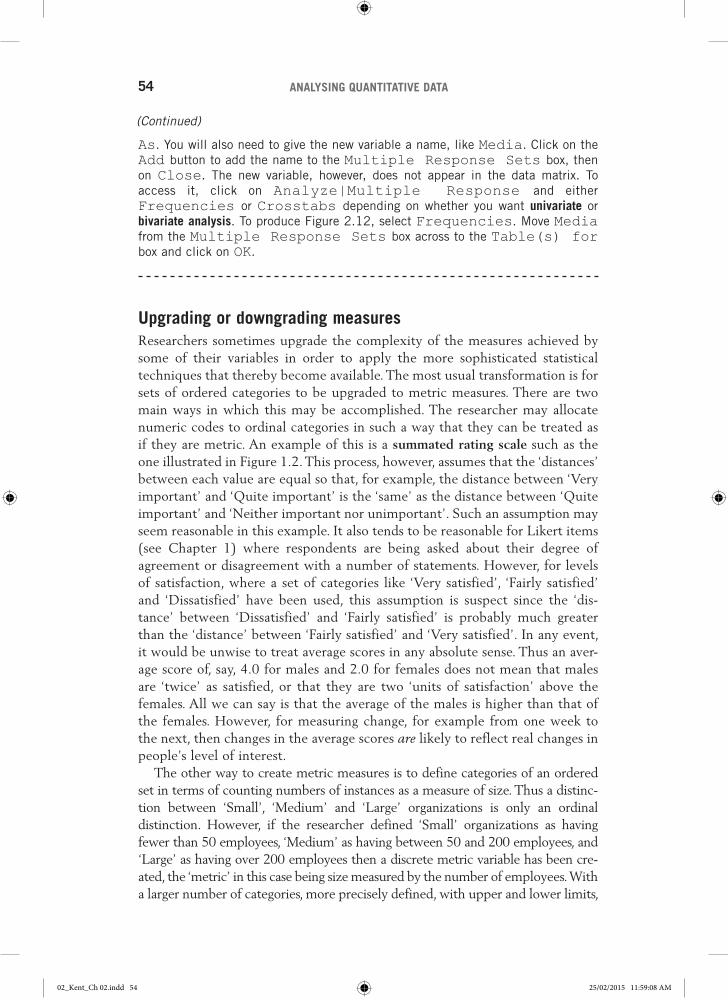
Multiple response questionsThere are often questions in a survey that allow respondents to pick more than one answer. The very first question on the alcohol survey, for example, asks respondents whether they have watched television, read a newspaper, read a magazine, listened to the radio or used the Internet in the last seven days. Respondents can reply ‘Yes’ to as many of these that apply. For the purpose of analysis, each medium will need to be treated as a separate variable, each one of which is either selected or not selected (so, it is binary). The five items then need to be analysed together. The results are shown in Figure 2.12. This indicates that there were 3,418 yeses. The 909 who indicated that they watched television constituted 26.6 per cent of the 3,418 yeses and 98.9 per cent of the 920 cases. Box 2.5 explains how to do this in SPSS.

02_Kent_Ch 02.indd 52 25/02/2015 11:59:07 AM

DATA PREPARATION 53

Box 2.5 Multiple response items in SPSS

To treat the five items relating to media consumption as a multiple response ques-tion, select Analyze|Multiple Response|Define sets. Bring the five variables across to the Variables in Set box. Since the code of 1 was entered for those who said ‘Yes’, enter 1 in the Counted Value box. Make sure the Dichotomies radio button is clicked under Variables Are Coded

Figure 2.11 The Compute Variable dialog box

Figure 2.12 SPSS multiple response

(Continued)

02_Kent_Ch 02.indd 53 25/02/2015 11:59:08 AM


As. You will also need to give the new variable a name, like Media. Click on the Add button to add the name to the Multiple Response Sets box, then on Close. The new variable, however, does not appear in the data matrix. To access it, click on Analyze|Multiple Response and either Frequencies or Crosstabs depending on whether you want univariate or bivariate analysis. To produce Figure 2.12, select Frequencies. Move Media from the Multiple Response Sets box across to the Table(s) for box and click on OK.

Upgrading or downgrading measuresResearchers sometimes upgrade the complexity of the measures achieved by some of their variables in order to apply the more sophisticated statistical techniques that thereby become available. The most usual transformation is for sets of ordered categories to be upgraded to metric measures. There are two main ways in which this may be accomplished. The researcher may allocate numeric codes to ordinal categories in such a way that they can be treated as if they are metric. An example of this is a summated rating scale such as the one illustrated in Figure 1.2. This process, however, assumes that the ‘distances’ between each value are equal so that, for example, the distance between ‘Very important’ and ‘Quite important’ is the ‘same’ as the distance between ‘Quite important’ and ‘Neither important nor unimportant’. Such an assumption may seem reasonable in this example. It also tends to be reasonable for Likert items (see Chapter 1) where respondents are being asked about their degree of agreement or disagreement with a number of statements. However, for levels of satisfaction, where a set of categories like ‘Very satisfied’, ‘Fairly satisfied’ and ‘Dissatisfied’ have been used, this assumption is suspect since the ‘dis-tance’ between ‘Dissatisfied’ and ‘Fairly satisfied’ is probably much greater than the ‘distance’ between ‘Fairly satisfied’ and ‘Very satisfied’. In any event, it would be unwise to treat average scores in any absolute sense. Thus an aver-age score of, say, 4.0 for males and 2.0 for females does not mean that males are ‘twice’ as satisfied, or that they are two ‘units of satisfaction’ above the females. All we can say is that the average of the males is higher than that of the females. However, for measuring change, for example from one week to the next, then changes in the average scores are likely to reflect real changes in people’s level of interest.

The other way to create metric measures is to define categories of an ordered set in terms of counting numbers of instances as a measure of size. Thus a distinc-tion between ‘Small’, ‘Medium’ and ‘Large’ organizations is only an ordinal distinction. However, if the researcher defined ‘Small’ organizations as having fewer than 50 employees, ‘Medium’ as having between 50 and 200 employees, and ‘Large’ as having over 200 employees then a discrete metric variable has been cre-ated, the ‘metric’ in this case being size measured by the number of employees. With a larger number of categories, more precisely defined, with upper and lower limits,

(Continued)

02_Kent_Ch 02.indd 54 25/02/2015 11:59:08 AM

DATA PREPARATION 55

it becomes possible to calculate an average size. This procedure is fine provided there is accurate information, for example, in the situation above, on the number of employees in each organization of interest. By creating (or assuming the crea-tion of) metric measures, the researcher can now, for example, add up and then calculate average scores, calculate standard deviations and use the variables in ways that will be explained in Chapters 4–6.

There are some circumstances when a researcher may downgrade a measure and treat it as if it were at a less complex level. Thus a metric variable may be treated as ranked by ignoring the distances between categories. A class test out of 100 may be used to create ranks of first, second, third, and so on. This may be undertaken by the researcher either because he or she feels that the assumptions of the original metric are unwarranted, or because the variable concerned is to be correlated with another ranked variable and the researcher wants to apply a statistic that requires two ranked variables. Metric variables can be ranked in SPSS using the procedure Transform|Rank Cases.

Another example of downgrading is when a researcher wishes to crosstabulate a nominal with an ordered category variable. An appropriate coefficient may be chosen that treats both variables as nominal, thereby ignoring the ordering of the categories in one of the variables. A more extreme example is when a researcher takes a continuous metric variable like age and groups respondents into a binary measure of ‘old’ and ‘young’ or into an ordered category measure of ‘old’, ‘middle aged’ and ‘young’. This may be undertaken if the researcher wishes to crosstabu-late age with another binary, nominal or ordered category variable, for example ‘purchased’ and ‘did not purchase’ a newspaper in the last seven days. The age split would normally be done in a way that creates two (or three or more as required) roughly equal groups. The SPSS procedure Transform|Compute can be used to create a new variable grouped in this way.

Handling missing values and ‘Don’t know’ responsesIn any survey, not all respondents will answer all the questions. This is less likely to be the result of individual refusal to answer some of the questions (although this does happen), or people accidentally omitting to consider some of the ques-tions, than a result of questionnaire design whereby not all the questions are relevant to all the respondents. The result is that values will be missing from some of the cells in the data matrix.

Where a question would be appropriate to a given respondent, but an answer is not recorded, then such missing values may be referred to as ‘item non-response’. Most researchers are inclined just to accept that there will be item non-response for some of the variables and will simply exclude them from the analysis. This is fine when the number of cases entered into the data matrix is large or at least sufficient for the kinds of analyses that are required. However, there is always the danger that this approach may reduce the number of cases used in a particular analysis to such an extent that meaningful analysis is not possible. There is, however, a bewildering array of techniques that have been suggested in the literature for ways of dealing with this situation. Most of these

02_Kent_Ch 02.indd 55 25/02/2015 11:59:08 AM


involve filling the gaps caused by missing values by finding an actual replace-ment value. The process is sometimes called ‘explicit imputation’ and the idea is to select a replacement value that is as similar as possible to the missing value. Where variables are metric, one remedial technique, for example, is to substitute the mean value for the missing value. For categorical variables one technique that is sometimes used is to give the questionnaire with the missing value the same value as the questionnaire immediately preceding it.

Most of the techniques assume, however, that question items not responded to are done so at random. This can be quite difficult to determine. Furthermore, when the amount of item non-response is small – less than about 5 per cent – then applying any of the methods is unlikely to make any significant difference to the interpretation of the data. Ideally, of course, researchers should, in report-ing their findings, communicate the nature and amount of item non-response in the dataset and describe the procedures used to remedy or cope with it. How missing values are handled in SPSS is explained in Box 2.6.

Box 2.6 Missing values in SPSS

SPSS makes a distinction between two kinds of missing value: system missing values and user-defined missing values. The former result when the person enter-ing the data has no value to enter for a particular variable (for whatever reason) for a particular case. In this situation the data analyst will just skip the cell and SPSS will enter a full stop in that cell to indicate that no value has been recorded. For most non-graphical outputs, SPSS will list in a separate Case Processing Summary the number of valid and the number of missing cases. In some tables, as in Figure 2.5 in an earlier section, valid and missing cases are shown in the printed output table itself. Percentages are then calcu-lated both for the total number of cases entered into the data matrix and for the total of non-missing cases for that variable – what SPSS calls the Valid Percent.

User-defined missing values are ones that have been entered into the data matrix, but the researcher decides to exclude them from the analysis. To create them for any particular variable, from the Variable View select the little blue box in the Missing column against the variable you want and obtain the Missing Values dialog box. This enables you either to pick out particular codes to be treated as missing values by clicking on the Discrete missing values radio button and entering up to three codes, or to select a range of missing values.

It would be a sensible policy to reserve system missing values in effect for ques-tions that are not applicable to the respondent in question and to give a special code for those where responses are missing for other reasons. The combination of system-defined and user-defined missing values can mean that, for some tables or calculations, the number of cases used is considerably less than the number of cases entered into the data matrix. Furthermore, it will mean that the number of

02_Kent_Ch 02.indd 56 25/02/2015 11:59:08 AM

DATA PREPARATION 57

cases included will vary from table to table or statistical analysis. If the number of cases in the data matrix is quite small to begin with, this can have serious implications for the analysis.

‘Don’t know’ answers are one type of non-committal reply that a respondent may give along with undecided or neutral responses in a balanced rating with a middle point. These responses may be built into the design of the questionnaire with explicit options for a non-committal response. In Figure 2.9, there are, for example, separate categories for ‘Neither important nor unimportant’ and for ‘Don’t know’: 285 or over 30 per cent gave a neutral response for the impor-tance of choosing well-known brands for chocolate or sweets, and 154 (over 16 per cent) indicated ‘Don’t know’ for cigarettes. In some questionnaires the ‘Don’t know’ answers are included in the ‘Neither’ category.

An understanding of the pattern of such replies is important for formulating research methodology, particularly questionnaire design, item phrasing or the sampling plan, or for interpreting the results when there are many ‘Don’t know’ responses. Non-committal replies have been interpreted very differently by researchers. These interpretations fit into two broad patterns:

•• ‘Don’t know’ responses are a valid indicator of the absence of attitudes, beliefs, opinions or knowledge.

•• ‘Don’t know’ replies are inaccurate reflections of existing cognitive states.

The first interpretation provides a rationale for including explicit non-committal response categories in the questionnaire. It also implies that such responses should be excluded from the analysis (treating them as user-defined missing val-ues in SPSS, see Box 2.6), even if this means that the number of cases on which the analysis is based is thereby reduced. If there are a lot of respondents in this category, then it is possible that the question to which people are being asked to respond is not well thought through and there may well be an argument for excluding the question from the analysis altogether.

The second interpretation has been used to set in motion various efforts to minimize ‘Don’t know’ responses on the basis that only committed responses will reflect a respondent’s true mental state. Such efforts will include providing ordered category measures that have no middle position or non-committal option, or that have interviewers probe each non-committal reply until a com-mittal response has been obtained.

If there are relatively few non-committal responses then leaving them out of the analysis may well be the best course of action to take, particularly if the number of remaining cases is still adequate for the statistical analyses being pro-posed. There will certainly be a case, however, for including them in any preliminary analysis of the variables. A decision can then be taken about whether they are to be excluded from subsequent analyses.

Survey research findings are certainly not invariant to decisions about what to do with non-committal responses. Treating such responses as randomly distrib-uted missing data points when in fact some responses are a genuine result of ambivalence or uncertainty may introduce bias into the data. The same would

02_Kent_Ch 02.indd 57 25/02/2015 11:59:08 AM


be true if responses are included as neutral positions when they are in fact an indicator of no opinion or refusal to answer. A first step in any analysis would be to investigate the extent to which non-committal responses are a function of demographic, behavioural or other cognitive variables. Some studies, for exam-ple, have reported an inverse relation between education and non-committal responses (the better educated are less prone to give them), but it has to be said that other research has found exactly the reverse. Durand and Lambert (1988) found that such responses vary systematically with socio-demographic charac-teristics and with involvement with the topic area.

Open-ended questionsMost surveys contain one or more open-ended questions where responses are recorded as words, phrases, sentences or even more extended text. To be used in quantitative data analysis, the responses need to be categorized and each cate-gory given a code. The result should be either a binary or a nominal measure such that the values are exhaustive and mutually exclusive, or a fuzzy set giving degrees of membership of a defined category.

The approach to coding can be split into two situations. In the first situation, the open-ended question is being used to capture factual information, since list-ing all the options for responses in a closed question would take up too much space. Where respondents can give their answer in numerical form, for example putting in their age, then no additional coding is necessary. The actual age can simply be put into the data matrix. Where responses are in words, like brand purchased last time, then coding will involve creating a list of all the possible answers, assigning a code to each and recording a code for each respondent’s answer. It may be necessary to develop coding rules which specify codes to be allocated when the answer does not fit any of the obvious categories. For exam-ple, if respondents are asked ‘Not counting yourself, how many other people were you with?’ then most will give a clear number, but some may say ‘30–40’ or ‘a lot’. In this situation, one rule might be to give the mid-point of a range of values, so the answer ‘30–40’ will be coded as 35.

Where open-ended questions are being used not to capture factual informa-tion but to record respondent opinions, attitudes, views, knowledge, and so on, then creating a sensible code frame is the most important part of the analysis. By definition this is likely to get quite complex – if it were easy then the ques-tion could no doubt be pre-coded! The aim is to formulate a set of categories that accurately represents the answers and where each category includes an appreciable number of responses. Ideally, the set of categories should be exhaustive, mutually exclusive and minimize the loss of information. Furthermore, they should be meaningful, consistent and relatively straightfor-ward to apply. There may also need to be separate codes for ‘No response’, ‘Not applicable’ and ‘Don’t know’. Where the information is very detailed there may need to be many codes.

02_Kent_Ch 02.indd 58 25/02/2015 11:59:08 AM

DATA PREPARATION 59

Developing a frame may require several ‘passes’ over the data. It is probably a good idea to have all the comments collected and typed out, but this may not be possible. A method of constant comparison is probably best. Begin by looking at a few of the comments and see whether they should be put into separate categories. Then look at a few more and see if some can be put into the same category or whether more categories will need to be developed. When too many categories begin to emerge, look for similarities so that some categories can be brought together. If there are a large number of responses then it may not be sensible to look through all of them to develop the fame, but take a sample. Thus if there are 500 cases, a sample of 50–100 should enable the frame to be finalized. It also helps if more than one person develops a code frame separately; they should then work together on a final code. This maximizes the validity and reliability of the process.

It helps if the researcher sets up the objectives for which the code frame is to be used before beginning the process. Thus if the objective is to look for positive and negative statements about a situation or a product then answers will be coded along this dimension, perhaps with categories of very positive, vaguely positive, mixed, vaguely negative and very negative. Sometimes answers to open-ended questions can be coded in several ways according to different dimensions. Thus a study of injuries following an earthquake could look at the way injuries occurred, the parts of the body affected, where the injury occurred, what the person was doing at the time, and so on. Each of these aspects may need to be recorded separately in a different variable.

At one time researchers had to code all open-ended questions before data entry could begin. With modern survey analysis packages like SPSS, however, this may be done after all the pre-coded questions have been entered. This is a big advantage because researchers are not always sure how responses to open-ended questions should be coded until they have started analysis of the data. In short, it is sometimes better to delay coding of open-ended responses until they are needed for analysis.

Key points and wider issues

Before engaging in the description of a dataset, or even following an initial overview of the distribution for each variable one at a time or each case one at a time, the researcher may wish to transform variables in a number of ways: for example, regrouping values on a nominal or ordered category measure to create fewer categories, creating class intervals from metric variables, com-puting totals or other scores from combinations of several variables, treating groups of variables as a multiple response question, upgrading or downgrading measures, handling missing values and non-committal responses, or coding open-ended questions. Some transformations might involve creating crisp or fuzzy set memberships as was explained in Chapter 1.

(Continued)

02_Kent_Ch 02.indd 59 25/02/2015 11:59:08 AM


Data transformation is an important part of the data analysis process. There are no ‘right’ or ‘wrong’ ways of engaging in data transformation and there are usually several different ways in which it can be done. Perhaps the best strat-egy is what is sometimes called ‘sensitivity analysis’, whereby transformations may be tried in different ways to see how sensitive the results are to such processes. This is particularly true for how missing cases and ‘Don’t know’ answers are handled.

Implications of this chapter for the alcohol marketing dataMany of the codings in the original dataset were illogical or inconsistent; for example, for some questions relating to whether or not they had done particular activities, respondents were given the choice between ‘Yes’, ‘No’ and ‘Don’t know’, while for others it was just ‘Yes’ and ‘No’. In a question asking respond-ents to indicate how often they had come across adverts for a range of different products, ‘Very often’ was coded 1 and ‘Never’ coded as 6, with ‘Don’t know’ as 7. Besides being counter-intuitive (the higher the score, the less often), this way of coding makes it impossible to use the codes as metric values for summation since ‘Don’t know’ has the highest value. Accordingly, a number of data transfor-mations were needed before analysis could begin. It was also necessary to create new variables additional to those in the questionnaire, for example the number of channels on which respondents had seen adverts for alcohol.

Chapter summaryBefore researchers can proceed with the next stages of data analysis, the data need to be prepared by checking questionnaires or other instruments of data capture for usability, editing responses for legibility, completeness and consistency, coding any responses that are not pre-coded, and assembling the data together by enter-ing all the values for all the variables for all the cases into a data matrix. Data entry into the survey analysis package SPSS was explained in some detail.

Before analysis of the data can begin, some of the variables may need to be transformed in various ways and decisions may have to be made about how to handle missing values. The careful preparation of data ready for analysis should never be neglected. If poor-quality data are entered into the analysis, then no matter how sophisticated the statistical techniques applied, a poor or untrust-worthy analysis will result. Handled with care, data preparation can substantially enhance the quality and usefulness of data analysis: paying inadequate attention to it can seriously compromise the validity of the results.

(Continued)

02_Kent_Ch 02.indd 60 25/02/2015 11:59:08 AM

DATA PREPARATION 61

Exercises and questions for discussion

1. To what extent can treating codes allocated to ordered category measures as if they are numeric values be justified in the data analysis process?

2. When transforming variables, researchers make many decisions for which there are no ‘rules’ or even rough guidelines. What impact might these decisions have on the validity of the data?

3. What are the key circumstances in which missing values might be a severe problem for the data analyst?

4. Open IBM SPSS on whatever system you are using and enter the nine key vari-ables for the first 12 cases for the alcohol marketing dataset that are illustrated in the next chapter in Figure 3.1. The procedures for doing so are explained in Box 2.1.

5. Figure 2.10 shows the total scores for the importance of well-known brands in choosing products. Try creating class intervals in various different ways using SPSS. The procedures for doing so are explained in Boxes 2.2 and 2.3.

6. Go to the website www.surveyresearch.weebly.com. Here you will find lots of inter-esting information about social surveys created by John Hall, previously Senior Research Fellow at the UK Social Science Research Council (1970–6) and Principal Lecturer in Sociology and Unit Director at the Survey Research Unit, Polytechnic of North London (1976–92). Download the Trinians dataset. Select Survey Unit, Social Science Research Council, then Surveys by SSRC Survey Unit and then the ‘Trinians’ survey. Read the back-ground to the survey, download the article in Folio and the questionnaire. Finally download and save the dataset from trinians.sav onto your SPSS file. Not all the questions in the questionnaire appear as variables and they are not all in the same order as in the questionnaire, but the question numbers are clearly marked. Check out the values being used from the Values column. Under Measure, they are all indicated as Scale. This is the default if researchers do not change any of these. Go down the variables and change to Ordinal or Nominal as appropri-ate (left click on Scale and the other two options will appear).

Further readingCragun, R. (2013) ‘Using SPSS and PASW’, Wikibooks. Available at http://en.wikibooks.

org/wiki/Using_SPSS_and_PASW.A useful (and free) wiki book giving a series of mini SPSS tutorials. For this chapter, have

a look through the section on basic operations.De Vaus, D. (2002) Analyzing Social Science Data: 50 Key Problems and Data Analysis.

London: Sage.Parts One and Two give quite detailed answers to frequently asked questions about data

preparation in the form of 15 problems like ‘How to code answers with multiple answers’.

Diamantopoulos, A. and Schlegelmilch, B. (1997) Taking the Fear Out of Data Analysis. London: Dryden Press. Republished by Cengage Learning, 2000.

Chapter 4 is about data preparation and transformation, but beware that the image of a data matrix is rather dated and does not look like an SPSS matrix.

02_Kent_Ch 02.indd 61 25/02/2015 11:59:08 AM


Suggested answers to the exercises and questions for discussion can be found at the end of this text, pp. 293–321, and on the companion website, (https://study.sagepub.com/kent), which also give links to relevant free online Sage journal articles, PowerPoint slides, an overview of data analysis packages, an introduction to SPSS and weblinks to alternative datasets.

02_Kent_Ch 02.indd 62 25/02/2015 11:59:08 AM

Documents

Analysing Quantitative Data