An efficient image segmentation algorithm for landscape analysis

www.elsevier.com/locate/jag

International Journal of Applied Earth Observation

and Geoinformation 6 (2004) 47–61

An efficient image segmentation algorithm

for landscape analysis

B.J. Devereuxa,*, G.S. Amablea, C. Costa Posadab

aUnit for Landscape Modelling, University of Cambridge, Mond Building, Free School Lane, Cambridge CB2 3RF, UKbDirector de Polıtica Ambiental, Departamento Nacional de Planeacion, Calle 26 No 13-19, Bogota, Colombia

Received 13 November 2003; accepted 7 July 2004

Abstract

Widespread development and use of object-based GIS in the environmental sciences has stimulated a rapid growth in demand

for parcel-based land cover data. Despite the fact that image segmentation techniques applied to remotely sensed data offer the

most effective and direct approach to generating such data their use is still restricted to specialist applications. This paper

describes a general purpose segmentation algorithm capable of creating parcel boundaries from a wide range of image types. A

brief review of image segmentation in a range of disciplines identifies key elements of a successful segmentation algorithm. The

structure and implementation of the algorithm is then described and its performance is illustrated using Landsat ETM imagery of

Eastern England. Comparison of the segmentation product generated by the algorithm with those generated by independent

human analysts demonstrates that the computer algorithm and the manually derived products have just less than eighty percent

correspondence. Most of the differences stem from the more detailed results achieved by the segmentation algorithm.

# 2004 Elsevier B.V. All rights reserved.

Keywords: Region growing; Image segmentation; Land cover; Edge detection; Cover parcels; Mixture modelling

1. Overview and objectives

The last decade has seen major progress in our

ability to extract land cover information from

remotely sensed data whether from space- or airborne

platforms. A vast number of classification algorithms

have been described in the literature and classification

products are widely used in a range of environmental

planning activities. With increasing use of Geogra-

* Corresponding author. Fax: +44 1223 763300.

E-mail address: [email protected] (B.J. Devereux).

0303-2434/$ – see front matter # 2004 Elsevier B.V. All rights reserved

doi:10.1016/j.jag.2004.07.007

phical Information Systems for land use applications

the demand for parcel-based land cover data has

grown rapidly. Furthermore, in the search for more

accurate classifiers there has been a growing recogni-

tion that so called ‘per pixel’ classifiers have inherent

limitations and a parcel-based approach can often lead

to more accurate classification. This growing demand

for parcel-based land cover data has been further

strengthened by developments in landscape ecology

which have revealed that an understanding of land-

scape structure as embodied in patchworks of land

cover polygons is fundamental in understanding many

.

B.J. Devereux et al. / International Journal of Applied Earth Observation and Geoinformation 6 (2004) 47–6148

ecosystems. The population performance and

dynamics of numerous animal species have been

related to land parcel or ‘patch’ properties such as

area, size, configuration and connectivity.

The need to acquire land cover parcel outlines for

large areas is thus fundamental to a wide range of

remote sensing applications both in the world of

environmental research and also in the context of

applied work such as mapping and environmental

planning. One method for extracting such data from

remotely sensed imagery is image segmentation.

Segmentation is the process of partitioning a digital

image into a set of discrete, non-overlapping regions on

the basis of internal homogeneity criteria. These may

be defined in terms of a simple measure such as image

contrast or may be the result of complex statistical

analysis. Either way, it is now well known that when

such regions have been extracted from satellite images

and aerial photographs, they form an excellent starting

point for subsequent geospatial analyses such as land

cover classification, mapping of landscape structure

and modelling of terrain attributes. Not unsurprisingly,

geoscientists have thus devoted considerable energy to

devising effective computational procedures for sol-

ving the image segmentation problem.

Given the range of applications for image

segmentation it is perhaps surprising that their use

as a basis for both land cover classification and

landscape ecological analyses has been relatively

limited. This is in part because the benefits of

segmentation procedures in these fields are only just

beginning to receive widespread recognition. Further-

more, software for image segmentation is not widely

available and many published algorithms are tailored

for specific rather than general applications. This

paper will describe a general purpose image segmen-

tation algorithm which has a proven track record for

delineation of land cover parcels and which can be

used in both landscape modelling and subsequent per-

parcel classification schemes.

A notable feature of the algorithm is its relative

simplicity. Many existing segmentors make substantial

demands on computing resources. Processing of even

small images (256 � 256 pixels) can require either

very large computers or substantial processing time or,

on some occasions, both. The algorithm described here

was designed and built for intensive use in applications

work. An important design criterion was thus the

ability to process full satellite image scenes (typically

6000 � 6000 pixels) on a PC workstation. As a

consequence, the temptation to include refinements

that might lead to a small improvement in performance

at the cost of substantial increase in processing time has

been resisted. The algorithm has been implemented in

the C programming language under the MS Visual

Studio C compiler. A Unix version is also available.

Typical execution times for a Landsat scene are less

than 30 minutes.

The remainder of this paper will present a brief

overview of image segmentation methods with

reference to their application in the geosciences. It

will then provide a description of the segmentation

algorithm followed by an example of how it can be

used for analysis of landscape structure. The example

involves segmenting an area of Eastern England

characterised by cover types ranging in complexity

from large scale patterns of arable farmland through

areas of semi-natural grassland and marsh to complex

urban and suburban areas. The paper will conclude

with an evaluation of segmentation performance.

2. Image segmentation methods and applications

In the last 20 years image segmentation has become

the focus of attention for a wide variety of disciplines

sharing a common need to extract useful information

from raster images. Early impetus for segmentation

research stemmed from the field of computer vision

with efforts to simulate the human brain’s ability to

understand photographs. This work was based on the

premise that the human mind interprets an image by

recognising distinct regions. Initially, the broad image

regions are recognised with subsequent focussing to

assimilate more and more detail (Marr, 1982). This

basic idea has persisted and forms the basis for

hierarchical approaches to image segmentation where

filtered and sub-sampled versions of the digital image

are arranged in a hierarchical data structure and

objects are extracted at increasing levels of detail from

successively lower levels of the tree.

With the rapid, widespread growth in availability of

raster scanning devices these basic ideas are now

being explored and applied in an enormous variety of

applications. Nunez and Llacer (2003) for example,

illustrate how segmentation of astronomical images

B.J. Devereux et al. / International Journal of Applied Earth Observation and Geoinformation 6 (2004) 47–61 49

using self-organizing neural networks can be used for

identification of stars. Li et al. (2003) show how

invariant features can be extracted from palm print

images for consistent alignment and identification.

Medical applications are extensive. Soltanian-Zadeh

et al. (2003) have used a clustering-based method to

identify stroke induced tissue damage in rats from

MRI images and Taur (2003) presents a segmentation

methodology for monitoring the extent of psoriasis

based on feature extraction and fuzzy data analysis. In

engineering Kim et al. (2003) describe a method for

analysing the shape and size of aggregate particles in

digital camera and laser profile data.

Applications in the geosciences revolve around two

principal requirements. Firstly, the vast quantities of

image data generated by earth orbiting satellites are

only of value for environmental analysis if they can be

converted to meaningful data via classification.

Secondly, the rapid growth and analytical power of

GIS systems have fuelled an enormous demand for

object-based information (Geneletti and Gorte, 2003).

By far the cheapest and richest source of such data is

segmentation and classification of remotely sensed

images derived from satellites or aircraft. Whilst

examples abound in meteorology, oceanography,

geology, cartography and the biosciences it is in the

area of land cover and landscape analysis that most

applications can be found.

Wicks et al. (2002) have highlighted the need for

accurate delineation of vegetation parcels to ensure

accurate evaluation of carbon sinks in studies of global

change. Numerous studies have focussed on the

segmentation of field patterns for use in crop inventory

and monitoring (See Benie and Thomson, 1992;

Meyer, 1992). Forestry applications aimed at measur-

ing stand canopy properties, biomass and health have

received extensive attention (Woodcock and Harward,

1992; Pekkarinen, 2002) as have efforts to map and

extract biophysical properties from tropical rain-

forests. Hill (1999) for example, reports that the use of

segmented Landsat TM imagery resulted in a major

improvement in ability to discriminate between

different forest types over basic per-pixel analysis.

In relation to soil moisture analysis Bosworth et al.

(2003) describe a segment-based approach to mapping

soil moisture using Landsat channels 3, 4 and 6 whilst

van der Sande et al. (2003) use segment-based

classification for evaluating flood risk.

Despite this strong body of evidence that image

segmentation can play a key role in object-based,

geospatial analysis the use of image segmentation

is rather less widespread than one might expect

(Lobo et al., 1996). Few of the leading image

analysis systems in remote sensing offer high quality

segmentation modules for use in classification

although demand from landscape ecologists is

contributing to the success of new products such

as ‘Ecognition’ which offer a sophisticated, seg-

ment-based approach to classification (Ecognition,

2002). One reason for this may be lack of awareness

of the benefits segment-based analysis can bring

coupled with a shortage of available software

implementations. An additional, more subtle pro-

blem perhaps relates to the diversity of applications

itself. Many of the studies referred to above relate to

very specific applications areas and as a conse-

quence, many published procedures in the geos-

ciences are tailored for specific needs.

One of the guiding principles in the work described

here has been to design a segmentor with the widest

possible range of applications in the environmental

sciences. Inevitably, this introduces the risk of less

than optimum performance in any specific application

but the present authors follow Woodcock and Harward

(1992) in being convinced of the need for a theory of

image structure for geospatial analysis. Such a theory

must take account of basic issues including resolution,

scale, scene noise and generalisation. It is only by

understanding the relationships between image struc-

ture and scene structure that such a theory will emerge

and this means that segmentation methods which

focus on image structure have a key role to play.

Frequent and comprehensive reviews of image

segmentation techniques (see for example Haralick

and Shapiro, 1985; Pal and Pal, 1993; Freixenet et al.,

2002) abound and these provide the background for

the technique described here.

For the purposes of this discussion it is convenient

to recognise three distinct approaches to image

segmentation which are a combination of the more

detailed, six category typology originally proposed by

Haralick and Shapiro (op. cit.). These are

1. m
easurement space clustering,
2. s
plit and merge techniques,
3. s
patial linkage procedures.


Measurement space clustering involves identifica-

tion of clusters in the measurement or feature space of

the image. One of the simplest approaches is to build

an image histogram and search for peaks and valleys.

Peaks are assumed to correspond with distinct objects

and valley low points are assumed to be their separ-

ation points. By selection of one or more appropriate

thresholds the image can be partitioned into homo-

genous objects which can be displayed by mapping

back into the image space. Density slicing is a simple

example of such a technique which reveals the main

weakness of the method for environmental applica-

tions. Most remotely sensed images are extremely

complex and the identification of thresholds which

give clean, well defined objects is almost impossible.

Other, more sophisticated variations on the

approach include statistical clustering methods such

as the ISODATA algorithm that groups pixels into

classes based on some measure of their distance apart

in feature space. Strictly speaking these are classifiers

rather than segmentors. Whilst they are frequently

used in the geosciences to segment images they suffer

from major shortcomings when used in this way. In

particular, failure to use spatial and contextual

information to determine the status of each pixel

tends to result in segmentations which have large

amounts of ‘salt and pepper’ noise and which result in

excessive merging of segments due to computational

constraints limiting the ultimate numbers of clusters

which can be identified.

Split and merge procedures work by treating an

entire image as an ‘existing’ segment. Existing

segments are split into quarters if they fail to meet

some homogeneity criterion based on greyscale

difference or segment variance. Continued splitting

results in a quad tree structure in which the leaves

represent the smallest segments. Such a structure

would clearly result in very square regions and to

avoid this the option of merging adjacent nodes in the

tree is introduced. This can be achieved by comparison

of greyscale intensity distributions using analysis of

variance. Cross et al. (1988) describe an early

implementation of this technique for analysis of

remotely sensed data and highlight its efficiency for

displaying versions of the original image at differing

levels of resolution.

The ability of split and merge approaches to store

multiple renditions of remotely sensed images at

different levels of generalisation has led to interest in

hierarchical segmentation. In these approaches it is

assumed that there is a relationship between object

boundaries at each level of generalisation thus leading

to the idea of nested, hierarchical scene models

proposed by Woodcock and Harward (op.cit.).

Examples of this approach are provided by Bosworth

et al. (2003) who employed a multi-resolution image

pyramid for watershed mapping and Benie and

Thomson (op.cit.) who achieved region merging on

the basis of adaptive similarity rules in their efforts to

segment agricultural landscapes.

By far the largest category of segmentation

methods is the spatial linkage techniques. These treat

each pixel in an image as a node in a graph. Adjacent

pixels which meet some similarity criterion are joined

by an arc and image segments are defined as maximal

sets of pixels belonging to the same connected

component (Haralick and Shapiro, op. cit.). Regions

are grown by systematically scanning the image.

Pixels which meet the similarity criterion are merged

and pixels which do not, form starting or ‘seed’ points

for new segments.

Usually, a simple, grey level difference is used as

the similarity criterion with adjacent pixels being

merged if they are within a greyscale difference

threshold. However, Baraldi and Parmiggiani (1996)

have shown that improved region growing can be

achieved when Landsat TM images are being

segmented by using a quantity called the ‘vector

degree of match’. This is based on a normalised and

adaptive comparison of pixel vectors rather than a

simple difference threshold. The great advantage of

linkage-based methods is their simplicity. However,

their main disadvantage is ‘region leakage’ where

segments leak out into their neighbours. Leakage

problems may arise as a consequence of beginning

new segments with excessively noisy pixels or may be

a consequence of the order in which image pixels are

processed. Either way, they result in serious problems

for subsequent analysis.

Numerous strategies have been devised to try and

circumvent the shortcomings of the simple linkage

approach. So called ‘hybrid linkage region growing’

recognises that it is important to avoid the inclusion of

edge pixels in the early stages of segment growth as

these are inherently noisy and lead to ill-conditioned

segments. Both Le Moigne and Tilton (1995) and


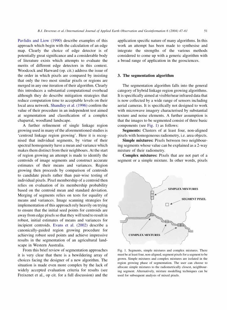
Fig. 1. Segments, simple mixtures and complex mixtures. There

must be at least four, non-aligned, segment pixels for a segment to be

grown. Simple mixtures and complex mixtures are isolated in the

region growing phase of segmentation. The user can choose to

allocate simple mixtures to the radiometrically closest, neighbour-

ing segment. Alternatively, mixture modelling techniques can be

used for subsequent analysis of mixed pixels.

Pavlidis and Liow (1990) describe examples of this

approach which begin with the calculation of an edge

map. Clearly the choice of edge detector is of

potentially great significance and a considerable body

of literature exists which attempts to evaluate the

merits of different edge detectors in this context.

Woodcock and Harward (op. cit.) address the issue of

the order in which pixels are compared by insisting

that only the two most similar pixels or regions are

merged in any one iteration of their algorithm. Clearly

this introduces a substantial computational overhead

although they do describe mitigation strategies that

reduce computation time to acceptable levels on their

local area network. Shandley et al. (1996) confirm the

value of their procedure in an independent test aimed

at segmentation and classification of a complex

chaparral, woodland landscape.

A further refinement of single linkage region

growing used in many of the aforementioned studies is

‘centroid linkage region growing’. Here it is recog-

nised that individual segments, by virtue of their

spectral homogeneity have a mean and variance which

makes them distinct from their neighbours. At the start

of region growing an attempt is made to identify the

centroids of image segments and construct accurate

estimates of their means and variances. Region

growing then proceeds by comparison of centroids

to candidate pixels rather than pair-wise testing of

individual pixels. Pixel membership of a centroid then

relies on evaluation of its membership probability

based on the centroid mean and standard deviation.

Merging of segments relies on tests for equality of

means and variances. Image scanning strategies for

implementation of this approach rely heavily on trying

to ensure that the initial seed points for centroids are

away from edge pixels so that they will tend to result in

robust, initial estimates of means and variances for

incipient centroids. Evans et al. (2002) describe a

canonically-guided region growing procedure for

achieving robust seed points and achieve impressive

results in the segmentation of an agricultural land-

scape in Western Australia.

From this brief review of segmentation approaches

it is very clear that there is a bewildering array of

choices facing the designer of a new algorithm. The

situation is made even more complex by the lack of

widely accepted evaluation criteria for results (see

Freixenet et al., op cit. for a full discussion) and the

application specific nature of many algorithms. In this

work an attempt has been made to synthesise and

integrate the strengths of the various methods

considered to come up with a generic algorithm with

a broad range of application in the geosciences.

3. The segmentation algorithm

The segmentation algorithm falls into the general

category of hybrid linkage region growing algorithms.

It is specifically aimed at visible/near infrared data that

is now collected by a wide range of sensors including

aerial cameras. It is specifically not designed to work

with microwave imagery characterised by substantial

texture and noise elements. A further assumption is

that the images to be segmented consist of three basic

components (see Fig. 1) as follows:

Segments: Clusters of at least four, non-aligned

pixels with homogeneous radiometry, i.e. area objects.

Simple mixtures: Pixels between two neighbour-

ing segments whose value can be explained as a 2-way

mixture of their radiometry.

Complex mixtures: Pixels that are not part of a

segment or a simple mixture. In other words, pixels


which are distinctive from their neighbours but cannot

be explained by a simple mixture of neighbouring

segments. These are mosaic pixels whose radiometry

is defined by more than two scene objects. They might

represent pixels covering the corner point of three

adjacent fields or a narrow linear feature such as a road

bounded by fields on either side.

This assumption has two important ramifications.

Firstly, it implies that scene objects occupying less

than four, non-aligned pixels cannot be identified by

the procedure as segments. Thus no attempt will be

made to extract scene objects which are too small to be

identified at the resolution of the sensor. Also it

provides a lower limit for specifying any minimum

mappable unit which might be required in subsequent

classification or analysis of the segments. Secondly, it

enables simple and complex mixed pixels to be

isolated in subsequent image analysis and treated

differently to area objects. Whilst many analyses

might simply follow the route of generalisation and

append these pixels to the closest segment, the

possibility of having hybrid classifiers based on both

per-pixel classification and linear mixture modelling is

opened up. It is this latter possibility which makes

segment-based classification so powerful.

Building on this basic assumption about the

structure of images, the segmentor has two key

stages. In the first stage an edge detection procedure is

used to label all pixels which would be unsuitable as

seed points for growing segments. In the second stage,

rectangular ‘seed regions’ are identified such that no

seed region contains an edge pixel. The seed regions

are then ordered in terms of their quality and grown

into segments using a recursive, centroid linkage

algorithm. The main features of the edge detection and

seeding/region growing stages will be described in the

following sub-sections.

3.1. Edge detection

By far the most common approach to generating

edge information for use in segmentation procedures

is the use of a conventional edge detection algorithm

applied to the image to be segmented (Pavlidis and

Liow, 1990). However, remotely sensed imagery

differs from that used in many other disciplines

because survey and cartographic data held in GIS

systems also has the potential to offer a source of edge

data (Janssen and Molenaar, 1995; Wicks et al., 2002).

Unfortunately both of these sources have problems

which result in noisy or incorrect edges and can lead to

difficulty for subsequent use by segmentors. Survey

data problems include poor image to map registration,

lack of temporal match, cartographic generalisation,

differences in scale and incomplete boundaries (e.g.

gates and gaps in hedgerows). Edge detectors suffer

from problems in the selection of appropriate thresh-

olds for splitting edge and non-edge pixels. This issue

can be particularly critical in segmentation algorithms

that use edge data for terminating the growth of

segments (see Le Moigne and Tilton, op. cit.).

Furthermore, there is such a plethora of edge detection

techniques now available, each with slightly differing

properties, that selection of an appropriate method can

also be difficult.

The segmentation algorithm described here has

been designed to work with both external survey data

rasterised into an edge map or with data generated by

any edge detection algorithm which results in a good,

but potentially imperfect structural representation of

the image in question. The main function of the edge

data is to ensure that well-behaved seed points can be

identified for subsequent region growing. Although

the edge data are used at the region growing stage they

are used for collateral checking of segment integrity

rather than as an absolute control over the process.

Taken together, these constraints on the use of edge

information mean that the segmentor is very robust in

the face of inaccurate edge information and a poor

quality edge map will not necessarily result in poor

quality segmentation.

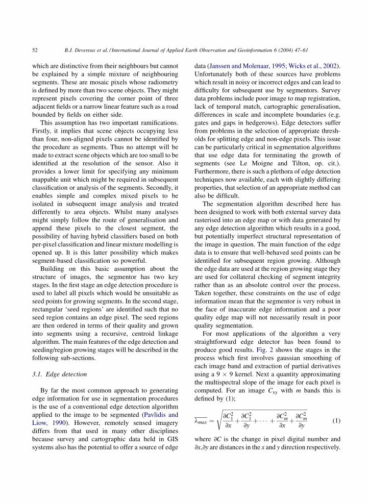
For most applications of the algorithm a very

straightforward edge detector has been found to

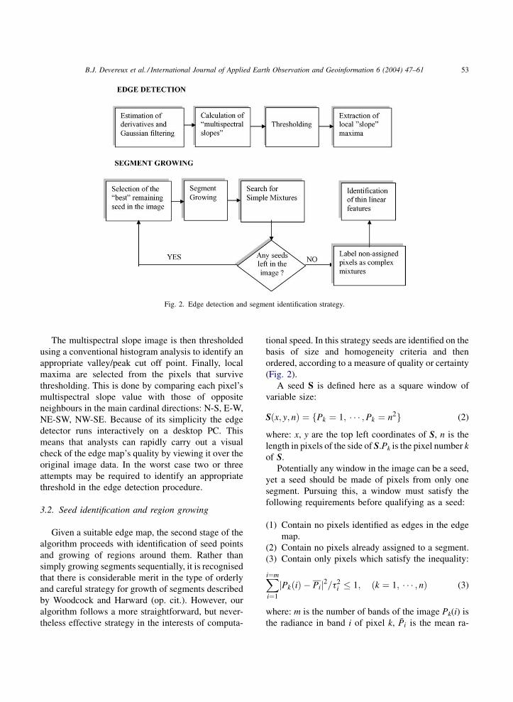
produce good results. Fig. 2 shows the stages in the

process which first involves gaussian smoothing of

each image band and extraction of partial derivatives

using a 9 � 9 kernel. Next a quantity approximating

the multispectral slope of the image for each pixel is

computed. For an image Cxy with m bands this is

defined by (1);

lmax ¼

ffiffiffiffiffiffiffiffiffiffiffiffiffiffiffiffiffiffiffiffiffiffiffiffiffiffiffiffiffiffiffiffiffiffiffiffiffiffiffiffiffiffiffiffiffiffiffiffiffiffiffiffiffiffiffiffiffiffiffiffi@C2

1

@xþ @C2

1

@yþ � � � þ @C2

m

@xþ @C2

m

@y

s(1)

where @C is the change in pixel digital number and

@x,@y are distances in the x and y direction respectively.


Fig. 2. Edge detection and segment identification strategy.

The multispectral slope image is then thresholded

using a conventional histogram analysis to identify an

appropriate valley/peak cut off point. Finally, local

maxima are selected from the pixels that survive

thresholding. This is done by comparing each pixel’s

multispectral slope value with those of opposite

neighbours in the main cardinal directions: N-S, E-W,

NE-SW, NW-SE. Because of its simplicity the edge

detector runs interactively on a desktop PC. This

means that analysts can rapidly carry out a visual

check of the edge map’s quality by viewing it over the

original image data. In the worst case two or three

attempts may be required to identify an appropriate

threshold in the edge detection procedure.

3.2. Seed identification and region growing

Given a suitable edge map, the second stage of the

algorithm proceeds with identification of seed points

and growing of regions around them. Rather than

simply growing segments sequentially, it is recognised

that there is considerable merit in the type of orderly

and careful strategy for growth of segments described

by Woodcock and Harward (op. cit.). However, our

algorithm follows a more straightforward, but never-

theless effective strategy in the interests of computa-

tional speed. In this strategy seeds are identified on the

basis of size and homogeneity criteria and then

ordered, according to a measure of quality or certainty

(Fig. 2).

A seed S is defined here as a square window of

variable size:

Sðx; y; nÞ ¼ fPk ¼ 1; � � � ;Pk ¼ n2g (2)

where: x, y are the top left coordinates of S, n is the

length in pixels of the side of S.Pk is the pixel number k

of S.

Potentially any window in the image can be a seed,

yet a seed should be made of pixels from only one

segment. Pursuing this, a window must satisfy the

following requirements before qualifying as a seed:

(1) C
ontain no pixels identified as edges in the edge
map.

(2) C
ontain no pixels already assigned to a segment.
(3) C
ontain only pixels which satisfy the inequality:
Xi¼m

jP ðiÞ Pij2=t2 � 1; ðk ¼ 1; � � � ; nÞ (3)
i¼1
k i

where: m is the number of bands of the image Pk(i) is

the radiance in band i of pixel k, Pi is the mean ra-


diance of S in band I, ti is a threshold specified by the

analyst in one of two ways: As a number of standard

deviations for the seed S in each band or as a constant

value for each band i of the entire image.

By restricting seeds to square blocks free of known

or suspected edge pixels, seeds are pushed away from

edges (even fragmented edges) towards the inside of

segments. When ti is specified as a constant then (3)corresponds to the simple linkage difference situation

and images can be processed which do not have

normally distributed segment radiometry. When ti is

specified in terms of standard deviations from the

seed’s mean, the assumption is implicitly made that

the segment in question is multivariate normal. Seeds

are generated which are tightly concentrated around

their radiometric mean and thus yield a good estimate

of the true segment mean for subsequent region

growing. This reduces the possibility of aberrant

segments being grown as a consequence of inap-

propriate starting pixels for segment growth.

The image is searched for seed points in such a way

that the largest seeds are identified first. A typical

starting size for most VIS/NIR satellite imagery would

be 15 � 15. All seeds of this size are identified and

grown into segments. Successively smaller seeds are

then processed until size 2 � 2 is reached. Because

large seeds give the best estimates of segment means

and standard deviations this search strategy tends to

maximise the reliability of the subsequent region

growing stage. A refinement of the search strategy

involves ordering all seeds of a particular size by their

standard deviation and processing those with the

smallest standard deviation first. Whilst this does

produce a slight improvement in performance the

additional computational costs are substantial and are

difficult to justify when dealing with production

situations where cost is an issue.

Growth of seeds into segments involves checking

neighbouring pixels in all directions. Pixels are added

to the segment if they meet the following require-

ments:

� T
hey are not assigned to another segment. (a) � T hey satisfy inequality (3) above (b) � T hey are not contained in the edge map. (c)
This process is performed using a recursive routine

that starts with a pixel in the middle of the seed. If the

pixel meets requirements (a) and (b), it is marked as

part of the growing segment. If it also fulfils requir-

ement (c), its four-connected neighbours (N, S, W, E)

are subsequently checked in order of distance from the

centre of the seed. Due to the four-connected, recu-

rsive approach, errors in the edge map are ignored and

the routine is able to grow around disconnected fea-

tures wrongly identified as edges. These are thus in-

cluded in the segment as long as requirements (a) and

(b) are satisfied. The region growing strategy enables

segments of any shape to be created. As a result of the

seed selection strategy and the recursive growing

routine, segments are grown from the biggest square

seed that can be fitted inside the segment, are not

affected by edge noise, are limited by clear continuous

edges and are radiometrically constrained by inequal-

ity (3).Finally, as each segment S is completed, all of its

perimeter pixels that neighbour a previously created

segment Sp are tested to see if they can be explained as

linear mixtures of S and Sp. Due to atmospheric noise

and the impact of processing methods such as

resampling, simple mixtures in satellite imagery can

be up to two pixels wide. For this reason, neighbouring

segments are allowed to be up to one pixel away from

the pixel being tested. Pixels identified as simple

mixtures are marked accordingly for subsequent

processing and all remaining pixels in the image are

assumed to be complex mixtures. Simple mixtures can

be either allocated to their radiometrically closest

neighbouring segment or could be decomposed using

linear mixture modelling techniques depending on the

application.

4. Performance evaluation: image segmentationand models of landscape structure

The algorithm described in this paper has been used

extensively over the last 5 years by both the authors

and a range of other institutions concerned with land

cover and associated issues (see Murfitt, 1999 for a

review). The types of imagery processed includes

CASI, ATM, LIDAR and aerial photography. Many of

the applications involve use of the segmentor as part

of a wider classification methodology aimed at the

production of parcel-based land cover maps. Fuller

et al. (2002) used our software implementation of


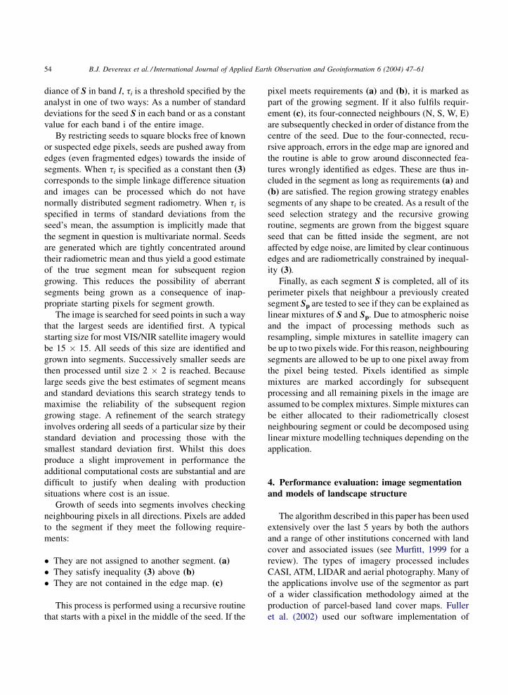
Fig. 3. The east of England study area.

the algorithm1 in the production of land cover 2000, a

Landsat TM/ETM based land cover map of the United

Kingdom. This work involved segmentation and

classification of some 79 images in a 2 year project.

The parcel-based approach made possible by image

segmentation was a key factor in producing a superior

product to its predecessor, the Land Cover Map of

Great Britain. Smith and Fuller (2001) describe a

similar approach to land cover classification in Jersey

which again underlines the value of the segmentor as

an element in classification methodology.

As these and other studies amply demonstrate the

value of the technique in image classification, this

paper will illustrate the performance of the algorithm

as a basis for extracting models of landscape structure

from Landsat ETM imagery. Recent developments in

landscape ecology have demonstrated very clearly that

the structure of landscapes, as defined by the pattern of

land cover parcels, corridors and matrix background

can have a profound influence on ecosystem function

(Forman, 1997). The result has been a substantial

increase in demand for mapping of land parcel and

corridor boundaries. However, manual recording of

such data from imagery is extremely time consuming

and rarely leads to products which are complete or

have consistent properties in terms of generalisation.

1 This software is distributed with Laserscan’s IGIS product or

can be obtained by contacting the University of Cambridge Unit for

Landscape Modelling.

Use of boundaries derived by raster to vector

conversion of classified images also has significant

problems stemming from classification errors,

unwanted merging of distinct segments which fall

into the same class and large numbers of unwanted

segments caused by erroneous classification of mixed

pixels.

By contrast image segmentation provides a direct

and effective approach to mapping landscape structure

by enabling the delineation of land cover parcels and

subsequently, their associated parameters (size, area,

connectivity, adjacency etc.). Furthermore, the seg-

mentation strategy described here permits effective

implementation of minimum mappable units and a

mechanism for dealing consistently with the problem

of mixed pixels. The aim of the evaluation experiment

was thus to compare the performance of the segmentor

as a basis for mapping landscape structure with

traditional visual interpretation.

The study site selected for the experiment was an

area of Eastern England stretching from the Thames

estuary in the south to the ports of Ipswich, Felixtowe

and Harwich in the north (Fig. 3). The diversity of

landscape types included in the area made it an

excellent example for testing the segmentor. The

dominant land use is one of large scale, arable farming

leading to a mosaic of large, clearly defined fields.

However, in terms of providing a challenge for the

algorithm, most of the remaining land covers are

rather more complex. In the north of the region there is


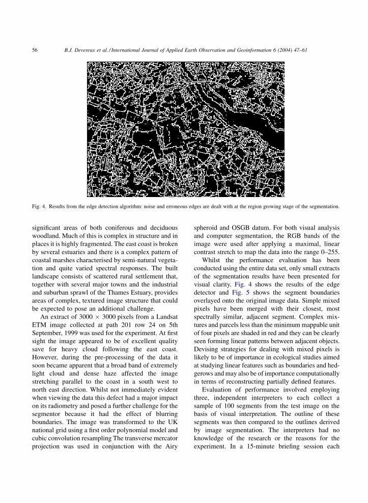
Fig. 4. Results from the edge detection algorithm: noise and erroneous edges are dealt with at the region growing stage of the segmentation.

significant areas of both coniferous and deciduous

woodland. Much of this is complex in structure and in

places it is highly fragmented. The east coast is broken

by several estuaries and there is a complex pattern of

coastal marshes characterised by semi-natural vegeta-

tion and quite varied spectral responses. The built

landscape consists of scattered rural settlement that,

together with several major towns and the industrial

and suburban sprawl of the Thames Estuary, provides

areas of complex, textured image structure that could

be expected to pose an additional challenge.

An extract of 3000 � 3000 pixels from a Landsat

ETM image collected at path 201 row 24 on 5th

September, 1999 was used for the experiment. At first

sight the image appeared to be of excellent quality

save for heavy cloud following the east coast.

However, during the pre-processing of the data it

soon became apparent that a broad band of extremely

light cloud and dense haze affected the image

stretching parallel to the coast in a south west to

north east direction. Whilst not immediately evident

when viewing the data this defect had a major impact

on its radiometry and posed a further challenge for the

segmentor because it had the effect of blurring

boundaries. The image was transformed to the UK

national grid using a first order polynomial model and

cubic convolution resampling The transverse mercator

projection was used in conjunction with the Airy

spheroid and OSGB datum. For both visual analysis

and computer segmentation, the RGB bands of the

image were used after applying a maximal, linear

contrast stretch to map the data into the range 0–255.

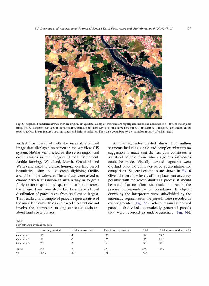
Whilst the performance evaluation has been

conducted using the entire data set, only small extracts

of the segmentation results have been presented for

visual clarity. Fig. 4 shows the results of the edge

detector and Fig. 5 shows the segment boundaries

overlayed onto the original image data. Simple mixed

pixels have been merged with their closest, most

spectrally similar, adjacent segment. Complex mix-

tures and parcels less than the minimum mappable unit

of four pixels are shaded in red and they can be clearly

seen forming linear patterns between adjacent objects.

Devising strategies for dealing with mixed pixels is

likely to be of importance in ecological studies aimed

at studying linear features such as boundaries and hed-

gerows and may also be of importance computationally

in terms of reconstructing partially defined features.

Evaluation of performance involved employing

three, independent interpreters to each collect a

sample of 100 segments from the test image on the

basis of visual interpretation. The outline of these

segments was then compared to the outlines derived

by image segmentation. The interpreters had no

knowledge of the research or the reasons for the

experiment. In a 15-minute briefing session each


Fig. 5. Segment boundaries drawn over the original image data. Complex mixtures are highlighted in red and account for 84.26% of the objects

in the image. Large objects account for a small percentage of image segments but a large percentage of image pixels. It can be seen that mixtures

tend to follow linear features such as roads and field boundaries. They also contribute to the complex mosaic of urban areas.

analyst was presented with the original, stretched

image data displayed on screen in the ArcView GIS

system. He/she was briefed on the seven major land

cover classes in the imagery (Urban, Settlement,

Arable farming, Woodland, Marsh, Grassland and

Water) and asked to digitise homogenous land parcel

boundaries using the on-screen digitising facility

available in the software. The analysts were asked to

choose parcels at random in such a way as to get a

fairly uniform spatial and spectral distribution across

the image. They were also asked to achieve a broad

distribution of parcel sizes from smallest to largest.

This resulted in a sample of parcels representative of

the main land cover types and parcel sizes but did not

involve the interpreters making conscious decisions

about land cover classes.

Table 1

Performance evaluation data

Over segmented Under segmented Ex

Operator 1 17 4 77

Operator 2 18 0 77

Operator 3 25 3 67

Total 60 7 221

% 20.8 2.4 76

As the segmentor created almost 1.25 million

segments including single and complex mixtures no

suggestion is made that the test data constitutes a

statistical sample from which rigorous inferences

could be made. Visually derived segments were

overlaid onto the computer-based segmentation for

comparison. Selected examples are shown in Fig. 6

Given the very low levels of line placement accuracy

possible with the screen digitising process it should

be noted that no effort was made to measure the

precise correspondence of boundaries. If objects

drawn by the interpreters were sub-divided by the

automatic segmentation the parcels were recorded as

over-segmented (Fig. 6c). Where manually derived

parcels sub-divided automatically generated parcels

they were recorded as under-segmented (Fig. 6b).

act correspondence Total Total correspondence (%)

98 78.6

95 81.0

95 70.5

288 76.7

.7 100


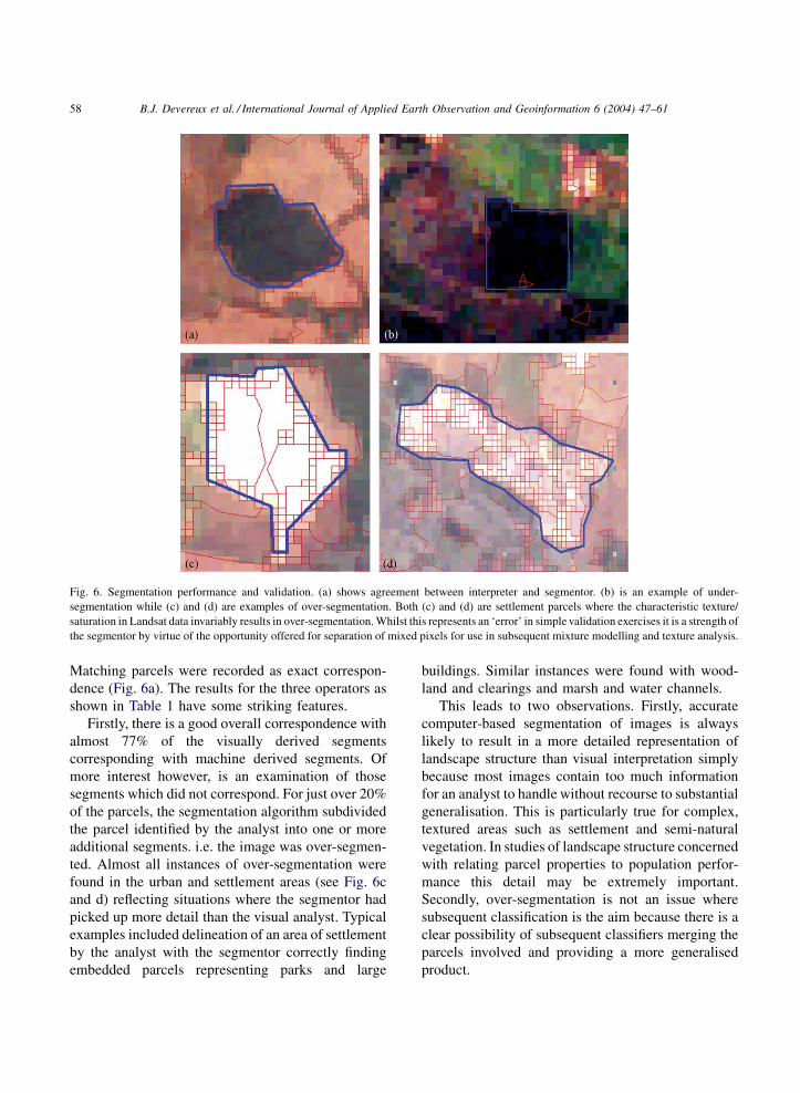
Fig. 6. Segmentation performance and validation. (a) shows agreement between interpreter and segmentor. (b) is an example of under-

segmentation while (c) and (d) are examples of over-segmentation. Both (c) and (d) are settlement parcels where the characteristic texture/

saturation in Landsat data invariably results in over-segmentation. Whilst this represents an ‘error’ in simple validation exercises it is a strength of

the segmentor by virtue of the opportunity offered for separation of mixed pixels for use in subsequent mixture modelling and texture analysis.

Matching parcels were recorded as exact correspon-

dence (Fig. 6a). The results for the three operators as

shown in Table 1 have some striking features.

Firstly, there is a good overall correspondence with

almost 77% of the visually derived segments

corresponding with machine derived segments. Of

more interest however, is an examination of those

segments which did not correspond. For just over 20%

of the parcels, the segmentation algorithm subdivided

the parcel identified by the analyst into one or more

additional segments. i.e. the image was over-segmen-

ted. Almost all instances of over-segmentation were

found in the urban and settlement areas (see Fig. 6c

and d) reflecting situations where the segmentor had

picked up more detail than the visual analyst. Typical

examples included delineation of an area of settlement

by the analyst with the segmentor correctly finding

embedded parcels representing parks and large

buildings. Similar instances were found with wood-

land and clearings and marsh and water channels.

This leads to two observations. Firstly, accurate

computer-based segmentation of images is always

likely to result in a more detailed representation of

landscape structure than visual interpretation simply

because most images contain too much information

for an analyst to handle without recourse to substantial

generalisation. This is particularly true for complex,

textured areas such as settlement and semi-natural

vegetation. In studies of landscape structure concerned

with relating parcel properties to population perfor-

mance this detail may be extremely important.

Secondly, over-segmentation is not an issue where

subsequent classification is the aim because there is a

clear possibility of subsequent classifiers merging the

parcels involved and providing a more generalised

product.


By contrast, under-segmentation is a greater

analytical problem. Where subsequent classification

is envisaged it is impossible for most widely used

classifiers to split the segments. For landscape

structure analyses the result is a clear error that

would contribute to over-estimation of parcel sizes in

landscape indices. In this examination only 2.4% of

the parcels checked were under-segmented. Most

cases were found to be situations where adjacent

arable fields containing the same crop had been split

by the visual analyst and merged by the segmentor.

Subsequent examination revealed that in these cases a

faint broken boundary could be discerned in the

image. The analyst had extrapolated the boundary

components into a complete feature and correctly

inferred the presence of two distinct fields. Such

extrapolation and inference is currently far beyond our

segmentor and whilst it may be claimed that human

operators cannot cope with the volume of data in even

medium resolution imagery, it is clear that computers

are a long way away from reproducing this type of

interpretation skill.

Clearly there are relatively small differences

between the results for each operator reflecting their

analytical skills, experience in image analysis and

sample composition. However, despite these differ-

ences the results are very consistent and demonstrate

in a simple way the performance of the segmentor.

Overall, it might be concluded that the segmentation

algorithm has done an excellent job at extracting a

model of landscape structure from the imagery in

question despite its defects and challenges. Whilst

there is a correspondence with visual interpretation of

around 77% it is clear that in most cases of over-

segmentation the algorithm is more accurate than the

analysts. It is only in the case of under segmented

parcels where there is a clear difficulty and these

account for less than 3% of the parcels processed

implying a real accuracy in excess of 97%.

5. Conclusions

Image segmentation algorithms can play a key role

in satisfying the demand for parcel based GIS data.

They also provide a mechanism for both improved

image classification systems and building patch,

corridor matrix models of landscapes. An efficient

computational algorithm has been described which

has a proven track record of performing well in all of

these applications areas. The algorithm has been

designed on the basis of a wide ranging review of

published procedures in a variety of disciplines

stretching beyond the environmental sciences. It can

process full satellite image scenes on a PC workstation

from a range of space and airborne sensors with

typical execution times of less than 30 minutes.

The algorithm embodies a two-stage procedure

based on edge detection followed by centroid linkage

region growing. Edges are used to enable the

identification of well- conditioned rectangular regions

that can be used for seeding a centroid linkage region

growing process. By using rectangular regions as

opposed to single pixels to start the growth of

segments, robust estimates of segment means and

standard deviations can be acquired and this enables

reliable, subsequent allocation of pixels to segments

based on membership probabilities. By ordering seeds

for processing in terms of a quality measure based on

size and homogeneity, an orderly pattern of region

growth is achieved in which leakage and other errors

are reduced. Systematic grey level trends within clearly

bounded objects are handled well by this process.

The segmentor assumes that remotely sensed

images can be decomposed into coherent regions

representing scene objects and that these regions are

separated by simple and complex mixed pixels which

form edges and areas of texture. These mixed pixels

lead to problems in most image classification systems

and the ability of the segmentor to isolate them for

differential treatment opens up new possibilities for

classification. Furthermore, its ability to deal with these

image features explicitly in terms of area enables

implementation of standards in the form of minimum

mappable units.

Several major classification studies have employed

the algorithm as part of their methodology and its value

in this context is well documented. This paper has thus

illustrated its value as a tool for mapping landscape

structure. A Landsat image covering an area of Eastern

England was segmented and despite the challenges of

complex land use patterns and cloud/haze affected

data, excellent results were achieved. Comparison of

segmented regions with those identified by three

independent visual interpreters revealed a 77%

correspondence in results. In a further 20% of instances


the algorithm produced a more detailed result than the

interpreters and in only 3% of cases did the algorithm

fail to find boundaries in the data which were of

operational significance.

These results demonstrate that computer based

image segmentation can play a key role in mapping of

landscape structure. Results are likely to be both more

consistent and significantly more detailed than those

achieved by visual interpretation. They are also

produced considerably faster and this is exemplified

by the fact that the entire segmentation process was

completed in about half of the time required by each

interpreter to collect the hundred test parcels used for

evaluation. In the very few situations where inference

was needed to arrive at the correct configuration of

boundaries, the analyst’s skills proved superior.

Building this type of inference into segmentation

procedures is perhaps the next major challenge facing

researchers in this field.

Acknowledgements

The contribution of both Leigh Carter and Tim

Mayo to the early development phase of the

segmentation algorithm has been an important

element of this work. More recently, the authors

gratefully acknowledge financial support from the

British National Space Centre provided as part of their

CLEVER mapping project. The patience and con-

structive comments of Geoff Smith and other

members of the Land Cover 2000 team at the NERC

Centre for Ecology and Hydrology is also acknowl-

edged. Thanks are due to colleagues at the ULM who

have helped to compile the evaluation data and others

who have also made key contributions. The efforts of

Tim Cockerell, Robin Fuller and Gill Renshaw are

also gratefully acknowledged. Finally, the authors

would like to thank Arko Lucieer and a second

anonymous referee whose constructive comments

have resulted in notable improvements to the paper.

References

Baraldi, A., Parmiggiani, F., 1996. Single linkage region growing

algorithms based on the vector degree of match. IEE Transact.

Geosci. Remote Sens. 34 (1), 137–147.

Benie, G., Thomson, K., 1992. Hierarchical image segmentation

using local and adaptive similarity rules. Int. J. Remote Sens. 13

(8), 1559–1570.

Bosworth, J., Koshimizu, T., Acton, S., 2003. Multi-resolution

segmentation of soil moisture imagery by watershed pyramids

with region merging. Int. J. Remote Sens. 24 (4), 741–

760.

Cross, A., Mason, D., Dury, S., 1988. Segmentation of remotely

sensed images by a split-and-merge process. Int. J. Remote Sens.

9, 1329–1345.

ECognition (2002). User Guide, Definiens Imaging GmbH, Munich,

p. 65. Available via http://www.definiens-imaging.com/pro-

duct.htm.

Evans, C., Jones, R., Svalbe, I., Berman, M., 2002. Segmenting

multispectral Landsat TM images into field units. IEEE Trans-

act. Geosci. Remote Sens. 40 (5), 1054–1064.

Forman, R.T., 1997. Land Mosaics. Cambridge University Press,

Cambridge.

Freixenet, J., Munoz, X., Raba, D., Marti, J., Cufi, X., 2002.

Yet another survey on image segmentation: Region and bound-

ary information integration. In: Heyden, A., et al. (Eds.), ECCV

Lecture Notes in Computer Science, vol. 2352. pp. 408–422.

Fuller, R., Smith, G., Sanderson, J., Hill, R., Thompson, A., 2002.

The UK land cover map 2000: construction of a parcel-based

vector map from satellite images. Cartogr. J. 39 (1), 15–25.

Geneletti, D., Gorte, B., 2003. A method for object-oriented land

cover classification combining Landsat TM data and aerial

photographs. Int. J. Remote Sens. 24 (6), 1273–1286.

Haralick, R., Shapiro, L., 1985. Image segmentation techniques.

Comput. Vis., Graph. Image Process. 29, 100–132.

Hill, R.A., 1999. Image segmentation for humid tropical forest

classification in Landsat TM data. Int. J. Remote Sens. 20

(5), 1039–1044.

Janssen, L., Molenaar, M., 1995. Terrain objects, their dynamics and

their monitoring by the integration of GIS and remote sensing.

IEEE Transact. Geosci. Remote Sens. 33 (3), 749–759.

Kim, H., Haas, C., Rauch, A., Browne, C., 2003. 3d image seg-

mentation of aggregates from laser profiling. Comput. Aid. Civil

Infrastruct. Eng. 18 (4), 254–263.

Le Moigne, J., Tilton, C., 1995. Refining image segmentation by

integration of edge and region data. IEEE Transact. Geosci.

Remote Sens. 33 (3), 605–615.

Li, W.X., Zhang, D., Xu, Z., 2003. Image alignment based on

invariant features for palmprint identification. Signal pro-

cess.–image commun. 18 (5), 373–379.

Lobo, A., Chic, O., Casterad, A., 1996. Classification of Mediter-

ranean crops with multisensor data: per-pixel versus per-object

statistics and image segmentation. Int. J. Remote Sens. 17 (12),

2385–2400.

Marr, D., 1982. Vision, Freeman, San Francisco.

Meyer, P., 1992. Segmentation and symbolic description for a

classification of agricultural areas with multispectral scanner

data. IEEE Transact. Geosci. Remote Sens. 30 (4), 673–

679.

Murfitt, P., 1999. Imagery in mapping. In: Nieuwenhuis, G.,

Vaughan, R., Molenaar, M. (Eds.), Operational Remote Sensing

for Sustainable Development. Balkema, pp. 363–366.

http://www.definiens-imaging.com/product.htm

http://www.definiens-imaging.com/product.htm


Nunez, J., Llacer, J., 2003. Astronomical image segmentation by

self-organizing neural networks and wavelets. Neural Netw. 16

(3–4), 411–417.

Pal, R., Pal, K., 1993. A review on image segmentation techniques.

Pattern Recognit. 26 (9), 1277–1294.

Pavlidis, T., Liow, Y., 1990. Integrating region growing and edge

detection. IEEE Transact. Pattern Anal. Machine Intell. 12 (3),

225–233.

Pekkarinen, A., 2002. A method for the segmentation of very high

spatial resolution images of forested landscapes. Int. J. Remote

Sens. 23 (14), 2817–2836.

Shandley, J., Franklin, J., White, T., 1996. Testing the Woodcock–

Harward image segmentation algorithm in an area of southern

California chaparral and woodland vegetation. Int. J. Remote

Sens. 17 (5), 983–1004.

Smith, G., Fuller, R., 2001. An integrated approach to land cover

classification: an example in the Island of Jersey. Int. J. Remote

Sens. 22 (16), 3123–3142.

Soltanian-Zadeh, H., Pasnoor, M., Hammoud, R., Jacobs, M., Patel,

S., Mitsias, P., Knight, R., Zheng, Z., Lu, M., Chopp, M., 2003.

MRI tissue characterization of experimental cerebral ischemia in

rat. J. Magn. Reson. Imaging 17 (4), 398–409.

Taur, J., 2003. Neuro-fuzzy approach to the segmentation of psor-

iasis images. J. VLSI Signal process. Syst. Signal Image Video

Technol. 35 (1), 19–27.

van der Sande, C.J., De Jong, S.M., De Roo, A.P.J., 2003. A

segmentation and classification approach of IKONOS-2 imagery

for land cover mapping to assist flood risk and flood damage

assessment. Int. J. Appl. Earth Observat. Geoinformat. 4 (3),

217–229.

Wicks, T., Smith, G., Curran, P., 2002. Polygon-based aggregation

of remotely-sensed data for regional ecological analyses. Int. J.

Appl. Earth Observat. Geoinformat. 4, 161–173.

Woodcock, C., Harward, V., 1992. Nested-hierarchical scene models

and image segmentation. Int. J. Remote Sens. 13 (16), 3167–

3187.

Documents

An efficient image segmentation algorithm for landscape analysis