1 Copyright © 2014 by ASME

Proceedings of the ASME 2014 33rd International Conference on Ocean, Offshore and Arctic Engineering OMAE2014

June 8-13, 2014, San Francisco, California, U.S.A.

OMAE2014-23437

AN ANALYSIS OF SLURRY TRANSPORT AT LOW LINE SPEEDS

Sape A. Miedema Offshore and Dredging Engineering

Delft University of Technology Delft, The Netherlands

ABSTRACT In Deep Sea Mining, material will be excavated at the sea

floor and transported to the surface. This transport always

consists of horizontal and vertical transport and can be carried

out mechanically or hydraulically. If the transport is

hydraulically, during the horizontal transport there is a danger of

bed formation and plugging the line. This is similar to the

horizontal transport in dredging with the difference that in deep-

sea mining the line length is much smaller, but also the line

speeds may be smaller. To avoid plugging the line, the line speed

has to be higher than a certain critical line speed. In literature

there are many theories about this critical line speed and about

bed forming in the pipe, but these theories are usually empirical

and cannot be applied under all circumstances. Different

particles sizes, pipe diameters and line speeds require different

equations, although a generic theory should cover everything.

For the critical velocity different definitions exist. Some

researchers use the definition that above the critical velocity no

bed, either stationary or sliding, exits. This definition is also

referred to as the limit deposit velocity. Others use the transition

between a stationary bed and a sliding bed as the definition of

the critical velocity. Whatever definition is used, the Moody

friction factor on the bed always plays an important role. Since

in literature no explicit formulation for this Moody friction factor

exists, an attempt is made to find an explicit formulation for the

Moody friction factor for the interface of the fluid flow and the

bed, where this interface consists of sheet flow.

INTRODUCTION

In slurry transport 4 main flow regimes can be

distinguished, the stationary or fixed bed regime, the sliding bed

regime, the heterogeneous regime and the homogeneous regime.

Ramsdell & Miedema (2013) subdivided this into 9 regimes also

distinguishing spatial and delivered volumetric concentration

curves. Based on the 4 main flow regimes the D-HL-LDV (Delft

Head Loss & Limit Deposit Velocity) model has been developed,

consisting of 4 sub models. The behavior of the fixed or

stationary bed regime is described in this paper, the behavior of

the sliding bed regime is described by Miedema & Ramsdell

(2014), the behavior of the homogeneous regime has been

described by Talmon (2013) and is used in a modified form,

while a possible solution for the heterogeneous flow regime has

been described by Miedema & Ramsdell (2013). The

heterogeneous flow regime is the flow regime where dredging

companies normally operate. At very high line speeds the

transition region between the heterogeneous regime and the

homogeneous regime can be reached. Since in deep sea mining

the pipe diameter, particle diameters, concentrations and line

speeds may be different from normal dredging operations, it is

important to know when a bed will occur. Thus the Moody

friction factor on the bed has to be determined more accurately.

The Wilson et al. (1992) model for the hydraulic transport

of solids in pipelines is a widely used model for the sliding bed

regime and will be used as a basis for the modelling. A

theoretical background of the model has been published piece by

piece in a number of articles over the years. A variety of

information provided in these publications makes the model

difficult to reconstruct.

A good understanding of the model structure is inevitable for the

user who wants to extend or adapt the model to specific slurry

flow conditions. The aim of this chapter is to summarize the

model theory and submit the results of the numerical analysis

carried out on the various model configurations. The numerical

results show some differences when compared with the

nomographs presented in the literature as the graphical

presentations of the generalized model outputs. Model outputs

are sensitive on a number of input parameters and on a model

configuration used. This chapter contains an overview of a

theory for the Wilson et al. (1992) two-layer model as it has been

published in a number of articles over the years. Results are

presented from the model computation. The results provide an

insight to the behavior of the mathematical model.

The model is based on an equilibrium of forces acting on the bed.

Driving forces and resisting forces can be distinguished. The

2 Copyright © 2014 by ASME

driving forces on the bed are the shear forces on the top of the

bed and the force resulting from the pressure times the bed cross

section. The pressure is the result of the sum of the shear force

on the pipe wall in the restricted area above the bed and the shear

force on the bed, divided by the cross section of this restricted

area. The resisting forces are the force as a result of the sliding

friction between the bed and the pipe wall and the viscous

friction force of the fluid between the particles in the bed and the

pipe wall. When the sum of the driving forces equals the sum of

the resisting forces, the so called limit deposit velocity is

reached. At line speeds below the limit deposit velocity, the bed

is stationary and does not move, because the driving forces are

smaller than the maximum resisting forces (maximum if the

sliding friction would be fully mobilized, which is not the case

at line speeds below the limit deposit velocity). At line speeds

above the limit deposit velocity, the bed is sliding with a speed

that is increasing with increasing line speed.

THE BASIC EQUATIONS FOR FLOW AND GEOMETRY

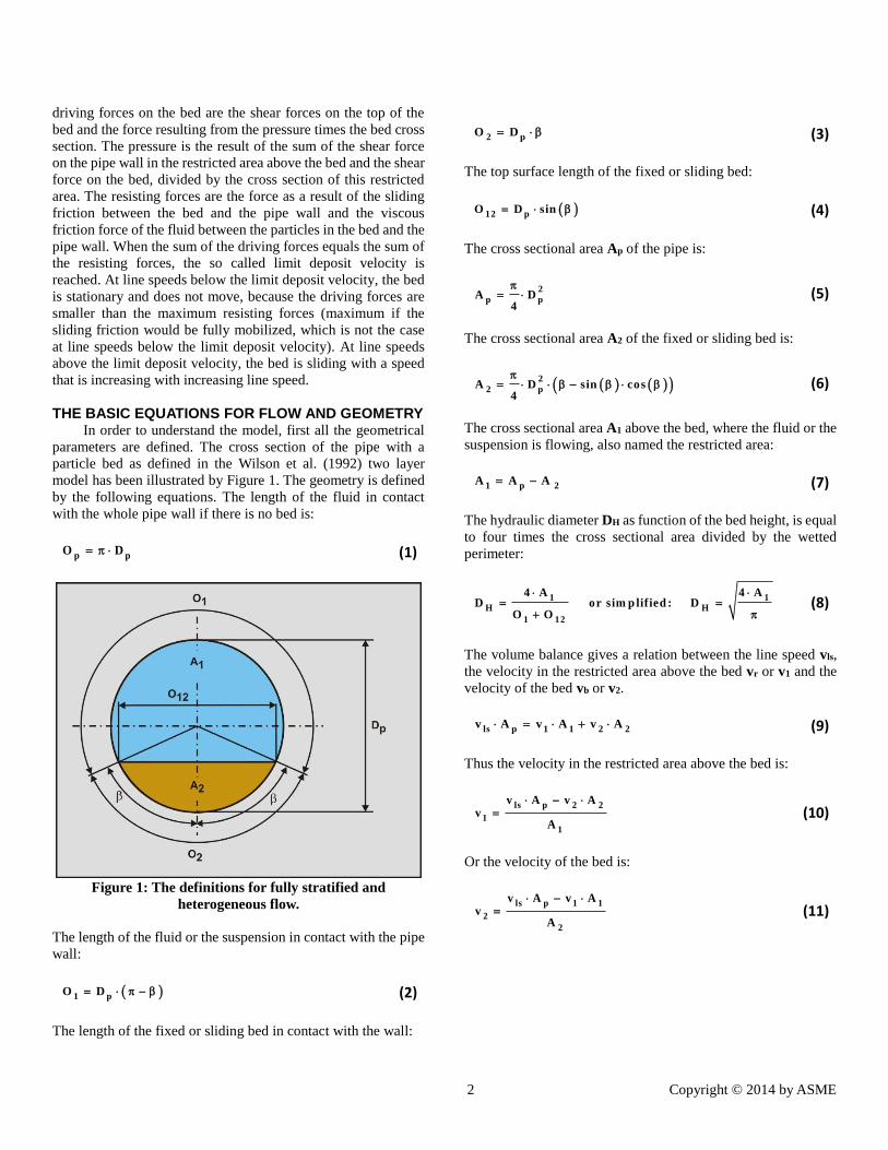
In order to understand the model, first all the geometrical

parameters are defined. The cross section of the pipe with a

particle bed as defined in the Wilson et al. (1992) two layer

model has been illustrated by Figure 1. The geometry is defined

by the following equations. The length of the fluid in contact

with the whole pipe wall if there is no bed is:

p pO D (1)

Figure 1: The definitions for fully stratified and

heterogeneous flow.

The length of the fluid or the suspension in contact with the pipe

wall:

1 pO D (2)

The length of the fixed or sliding bed in contact with the wall:

2 pO D (3)

The top surface length of the fixed or sliding bed:

12 pO D sin (4)

The cross sectional area Ap of the pipe is:

2

p pA D4

(5)

The cross sectional area A2 of the fixed or sliding bed is:

2

2 pA D sin cos4

(6)

The cross sectional area A1 above the bed, where the fluid or the

suspension is flowing, also named the restricted area:

1 p 2A A A (7)

The hydraulic diameter DH as function of the bed height, is equal

to four times the cross sectional area divided by the wetted

perimeter:

1 1H H

1 12

4 A 4 AD or sim p lified : D

O O

(8)

The volume balance gives a relation between the line speed vls,

the velocity in the restricted area above the bed vr or v1 and the

velocity of the bed vb or v2.

ls p 1 1 2 2v A v A v A (9)

Thus the velocity in the restricted area above the bed is:

ls p 2 2

1

1

v A v Av

A

(10)

Or the velocity of the bed is:

ls p 1 1

2

2

v A v Av

A

(11)

3 Copyright © 2014 by ASME

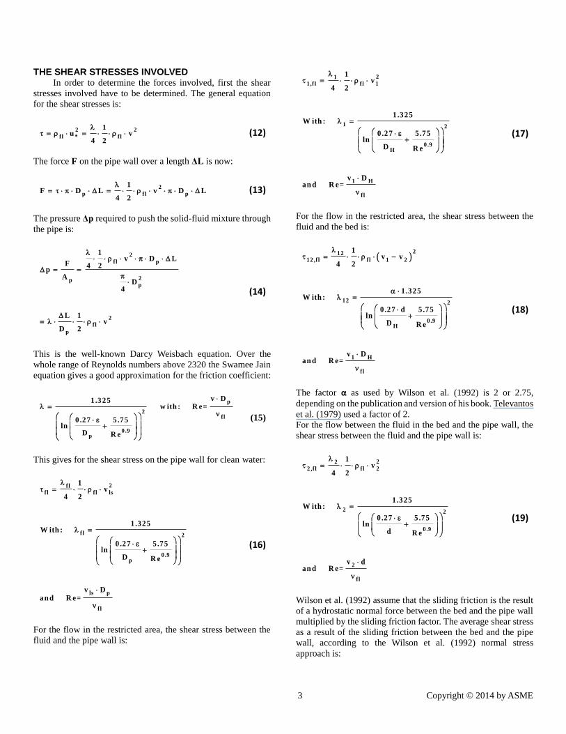
THE SHEAR STRESSES INVOLVED In order to determine the forces involved, first the shear

stresses involved have to be determined. The general equation

for the shear stresses is:

2 2

fl * fl

1u v

4 2

(12)

The force F on the pipe wall over a length ΔL is now:

2

p fl p

1F D L v D L

4 2

(13)

The pressure Δp required to push the solid-fluid mixture through

the pipe is:

2

fl p

2pp

2

fl

p

1v D L

F 4 2p

AD

4

L 1v

D 2

(14)

This is the well-known Darcy Weisbach equation. Over the

whole range of Reynolds numbers above 2320 the Swamee Jain

equation gives a good approximation for the friction coefficient:

p

2fl

0 .9p

v D1.325 w ith : R e=

0.27 5 .75ln

D R e

(15)

This gives for the shear stress on the pipe wall for clean water:

2flfl fl ls

fl 2

0 .9p

ls p

fl

1v

4 2

1 .325W ith :

0 .27 5 .75ln

D R e

v Dan d R e=

(16)

For the flow in the restricted area, the shear stress between the

fluid and the pipe wall is:

211,fl fl 1

1 2

0 .9H

1 H

fl

1v

4 2

1 .325W ith :

0 .27 5 .75ln

D R e

v Dan d R e=

(17)

For the flow in the restricted area, the shear stress between the

fluid and the bed is:

212

12 ,fl fl 1 2

12 2

0 .9H

1 H

fl

1v v

4 2

1 .325W ith :

0 .27 d 5 .75ln

D R e

v Dan d R e=

(18)

The factor α as used by Wilson et al. (1992) is 2 or 2.75,

depending on the publication and version of his book. Televantos

et al. (1979) used a factor of 2.

For the flow between the fluid in the bed and the pipe wall, the

shear stress between the fluid and the pipe wall is:

222 ,fl fl 2

2 2

0 .9

2

fl

1v

4 2

1 .325W ith :

0 .27 5 .75ln

d R e

v dan d R e=

(19)

Wilson et al. (1992) assume that the sliding friction is the result

of a hydrostatic normal force between the bed and the pipe wall

multiplied by the sliding friction factor. The average shear stress

as a result of the sliding friction between the bed and the pipe

wall, according to the Wilson et al. (1992) normal stress

approach is:

4 Copyright © 2014 by ASME

fr fl sd vb p

2 ,fr

p

g R C A

D

2 sin cos

(20)

It is however also possible that the sliding friction force results

from the weight of the bed multiplied by the sliding friction

factor. For low volumetric concentrations, there is not much

difference between the two methods, but at higher volumetric

concentrations there is.The average shear stress as a result of the

sliding friction between the bed and the pipe wall, according to

the weight normal stress approach is:

fr fl sd vb p

2 ,fr

p

g R C A

D

sin cos

(21)

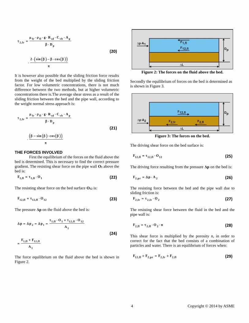
THE FORCES INVOLVED First the equilibrium of the forces on the fluid above the

bed is determined. This is necessary to find the correct pressure

gradient. The resisting shear force on the pipe wall O1 above the

bed is:

1,fl 1,fl 1F O (22)

The resisting shear force on the bed surface O12 is:

12 ,fl 12 ,fl 12F O (23)

The pressure Δp on the fluid above the bed is:

1,fl 1 12 ,fl 12

2 1

1

1,fl 12 ,fl

1

O Op p p

A

F F

A

(24)

The force equilibrium on the fluid above the bed is shown in

Figure 2.

Figure 2: The forces on the fluid above the bed.

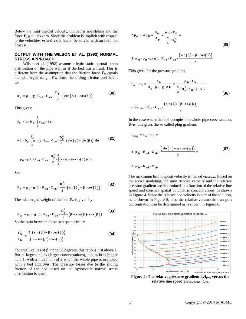
Secondly the equilibrium of forces on the bed is determined as

is shown in Figure 3.

Figure 3: The forces on the bed.

The driving shear force on the bed surface is:

12 ,fl 12 ,fl 12F O (25)

The driving force resulting from the pressure Δp on the bed is:

2 ,pr 2F p A (26)

The resisting force between the bed and the pipe wall due to

sliding friction is:

2 ,fr 2 ,fr 2F O (27)

The resisting shear force between the fluid in the bed and the

pipe wall is:

2 ,fl 2 ,fl 2F O n (28)

This shear force is multiplied by the porosity n, in order to

correct for the fact that the bed consists of a combination of

particles and water. There is an equilibrium of forces when:

12 ,fl 2 ,pr 2 ,fr 2 ,flF F F F (29)

5 Copyright © 2014 by ASME

Below the limit deposit velocity, the bed is not sliding and the

force F2,fl equals zero. Since the problem is implicit with respect

to the velocities v1 and v2, it has to be solved with an iteration

process.

OUTPUT WITH THE WILSON ET AL. (1992) NORMAL STRESS APPROACH

Wilson et al. (1992) assume a hydrostatic normal stress

distribution on the pipe wall as if the bed was a fluid. This is

different from the assumption that the friction force Ffr equals

the submerged weight FW times the sliding friction coefficient

μfr.

p

n fl sd vb

Dg R C cos cos

2

(30)

This gives:

N p s ,N

0

2

p

p fl sd vb

0

2

p

fl sd vb

0

F L D d

DL D g R C cos cos d

2

Dg L R C cos cos d

2

(31)

So:

2

p

N fl sd vb

DF g L R C sin cos

2

(32)

The submerged weight of the bed Fw is given by:

2

p

W fl sd vb

DF g L R C sin cos

4

(33)

So the ratio between these two quantities is:

N

W

2 sin cosF

F sin cos

(34)

For small values of β, up to 60 degrees, this ratio is just above 1.

But at larges angles (larger concentrations), this ratio is bigger

than 1, with a maximum of 2 when the whole pipe is occupied

with a bed and β=π. The pressure losses due to the sliding

friction of the bed based on the hydrostatic normal stress

distribution is now:

fr Nfrm fl

2pp

fr fl sd vb

FFp p

AD

4

sin cos2 g L R C

(35)

This gives for the pressure gradient:

fr Nfrm fl

2p flp fl

fr sd vb

FFi i

A g LD g L

4

sin cos2 R C

(36)

In the case where the bed occupies the whole pipe cross section,

β=π, this gives the so called plug gradient:

p lu g m fl

fr sd vb

fr sd vb

i i i

s in cos2 R C

2 R C

(37)

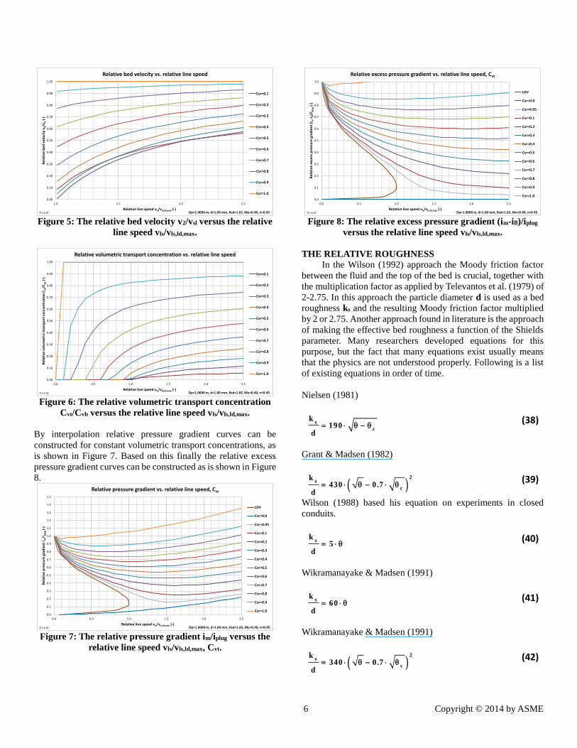
The maximum limit deposit velocity is named vls,ld,max. Based on

the above modeling, the limit deposit velocity and the relative

pressure gradient are determined as a function of the relative line

speed and constant spatial volumetric concentrations, as shown

in Figure 4. Since the relative bed velocity is part of the solution,

as is shown in Figure 5, also the relative volumetric transport

concentration can be determined as is shown in Figure 6.

Figure 4: The relative pressure gradient im/iplug versus the

relative line speed vls/vls,ld,max, Cvs.

0.0

0.1

0.2

0.3

0.4

0.5

0.6

0.7

0.8

0.9

1.0

1.1

1.2

1.3

1.4

1.5

0.0 0.5 1.0 1.5 2.0 2.5

Rel

ativ

e p

ress

ure

gra

die

nt

i m/i

plu

g(-

)

Relative line speed vls/vls,ld,max (-)

Relative pressure gradient vs. relative line speed, Cvs

LDV

Cvr=0.0

Cvr=0.1

Cvr=0.2

Cvr=0.3

Cvr=0.4

Cvr=0.5

Cvr=0.6

Cvr=0.7

Cvr=0.8

Cvr=0.9

Cvr=1.0

© S.A.M. Dp=1.0000 m, d=1.00 mm, Rsd=1.65, Mu=0.40, n=0.45

6 Copyright © 2014 by ASME

Figure 5: The relative bed velocity v2/vsl versus the relative

line speed vls/vls,ld,max.

Figure 6: The relative volumetric transport concentration

Cvt/Cvb versus the relative line speed vls/vls,ld,max.

By interpolation relative pressure gradient curves can be

constructed for constant volumetric transport concentrations, as

is shown in Figure 7. Based on this finally the relative excess

pressure gradient curves can be constructed as is shown in Figure

8.

Figure 7: The relative pressure gradient im/iplug versus the

relative line speed vls/vls,ld,max, Cvt.

Figure 8: The relative excess pressure gradient (im-ifl)/iplug

versus the relative line speed vls/vls,ld,max.

THE RELATIVE ROUGHNESS

In the Wilson (1992) approach the Moody friction factor

between the fluid and the top of the bed is crucial, together with

the multiplication factor as applied by Televantos et al. (1979) of

2-2.75. In this approach the particle diameter d is used as a bed

roughness ks and the resulting Moody friction factor multiplied

by 2 or 2.75. Another approach found in literature is the approach

of making the effective bed roughness a function of the Shields

parameter. Many researchers developed equations for this

purpose, but the fact that many equations exist usually means

that the physics are not understood properly. Following is a list

of existing equations in order of time.

Nielsen (1981)

s

c

k190

d (38)

Grant & Madsen (1982)

2

s

c

k430 0.7

d (39)

Wilson (1988) based his equation on experiments in closed

conduits.

sk

5d

(40)

Wikramanayake & Madsen (1991)

sk

60d

(41)

Wikramanayake & Madsen (1991)

2

s

c

k340 0.7

d (42)

0.00

0.10

0.20

0.30

0.40

0.50

0.60

0.70

0.80

0.90

1.00

1.0 1.5 2.0 2.5

Re

lati

ve b

ed

ve

loci

ty v

2/v

ls(-

)

Relative line speed vls/vls,ld,max (-)

Relative bed velocity vs. relative line speed

Cvr=0.1

Cvr=0.2

Cvr=0.3

Cvr=0.4

Cvr=0.5

Cvr=0.6

Cvr=0.7

Cvr=0.8

Cvr=0.9

Cvr=1.0

© S.A.M. Dp=1.0000 m, d=1.00 mm, Rsd=1.65, Mu=0.40, n=0.45

0.00

0.10

0.20

0.30

0.40

0.50

0.60

0.70

0.80

0.90

1.00

0.0 0.5 1.0 1.5 2.0 2.5

Rel

ativ

e vo

lum

etri

c tr

ansp

ort

co

nce

ntr

atio

n C

vt/C

vb(-

)

Relative line speed vls/vls,ld,max (-)

Relative volumetric transport concentration vs. relative line speed

Cvr=0.1

Cvr=0.2

Cvr=0.3

Cvr=0.4

Cvr=0.5

Cvr=0.6

Cvr=0.7

Cvr=0.8

Cvr=0.9

Cvr=1.0

© S.A.M. Dp=1.0000 m, d=1.00 mm, Rsd=1.65, Mu=0.40, n=0.45

0.0

0.1

0.2

0.3

0.4

0.5

0.6

0.7

0.8

0.9

1.0

1.1

1.2

1.3

1.4

1.5

0.0 0.5 1.0 1.5 2.0 2.5

Rel

ativ

e p

ress

ure

gra

die

nt

i m/i

plu

g(-

)

Relative line speed vls/vls,ld,max (-)

Relative pressure gradient vs. relative line speed, Cvt

LDV

Cvr=0.0

Cvr=0.05

Cvr=0.1

Cvr=0.2

Cvr=0.3

Cvr=0.4

Cvr=0.5

Cvr=0.6

Cvr=0.7

Cvr=0.8

Cvr=0.9

Cvr=1.0

© S.A.M. Dp=1.0000 m, d=1.00 mm, Rsd=1.65, Mu=0.40, n=0.45

0.0

0.1

0.2

0.3

0.4

0.5

0.6

0.7

0.8

0.9

1.0

0.0 0.5 1.0 1.5 2.0 2.5

Rel

ativ

e ex

cess

pre

ssu

re g

rad

ien

t (i

m-i

fl)/

i plu

g(-

)

Relative line speed vls/vls,ld,max (-)

Relative excess pressure gradient vs. relative line speed, Cvt

LDV

Cvr=0.0

Cvr=0.05

Cvr=0.1

Cvr=0.2

Cvr=0.3

Cvr=0.4

Cvr=0.5

Cvr=0.6

Cvr=0.7

Cvr=0.8

Cvr=0.9

Cvr=1.0

© S.A.M. Dp=1.0000 m, d=1.00 mm, Rsd=1.65, Mu=0.40, n=0.45

7 Copyright © 2014 by ASME

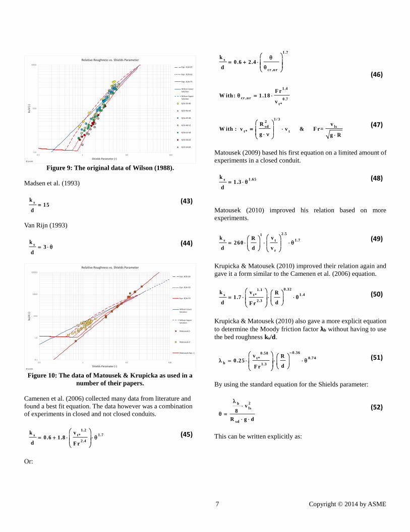
Figure 9: The original data of Wilson (1988).

Madsen et al. (1993)

sk

15d

(43)

Van Rijn (1993)

sk

3d

(44)

Figure 10: The data of Matousek & Krupicka as used in a

number of their papers.

Camenen et al. (2006) collected many data from literature and

found a best fit equation. The data however was a combination

of experiments in closed and not closed conduits.

1.2

1 .7s t*

2 .4

k v0.6 1 .8

d F r

(45)

Or:

1 .7

s

cr ,u r

1 .4

cr ,u r 0 .7

t*

k0.6 2 .4

d

F rW ith : 1 .18

v

(46)

1 / 3

2

sd ls

t* t

R vW ith : v v & F r=

g g R

(47)

Matousek (2009) based his first equation on a limited amount of

experiments in a closed conduit.

1.65sk

1.3d

(48)

Matousek (2010) improved his relation based on more

experiments.

2 .51

1 .7s t

r

k vR260

d d v

(49)

Krupicka & Matousek (2010) improved their relation again and

gave it a form similar to the Camenen et al. (2006) equation.

0.321.1

1 .4s t*

2 .3

k v R1.7

d dF r

(50)

Krupicka & Matousek (2010) also gave a more explicit equation

to determine the Moody friction factor λb without having to use

the bed roughness ks/d.

0.360.58

0.74t*

b 1.3

v R0.25

dF r

(51)

By using the standard equation for the Shields parameter:

2b

ls

sd

v8

R g d

(52)

This can be written explicitly as:

1.0

10.0

100.0

0.1 1 10 100

ks/d

(-)

Shields Parameter (-)

Relative Roughness vs. Shields Parameter

Eqn. R/d=35

Eqn. R/d=55

Eqn. R/d=75

Wilson LowerSolution

Wilson UpperSolution

R/d=30-40

R/d=40-43

R/d=43-48

R/d=48-52

R/d=52-58

R/d=58-64

R/d=64-83

© S.A.M.

0.1

1.0

10.0

100.0

1000.0

0.1 1 10 100

ks/d

(-)

Shields Parameter (-)

Relative Roughness vs. Shields Parameter

Eqn. R/d=35

Eqn. R/d=55

Eqn. R/d=75

Wilson LowerSolution

Wilson UpperSolution

Matousek 1

Matousek 2

Matousek Eqn. 1

© S.A.M.

8 Copyright © 2014 by ASME

0.74

20.360 .58 ls

0 .26 t*

b 1.3sd

1v

v R 80.25

d R g dF r

(53)

Whether this is the purpose of this equation is not clear, but

mathematically it’s correct.

Camenen & Larson (2013) wrote a technical note on the

accuracy of equivalent roughness height formulas in practical

applications. They already concluded that most equations are

based on a relation between the relative roughness ks/d and the

Shields parameter.

The relative roughness is a parameter that often has nothing to

do with the real roughness of the bed, but it is a parameter to use

in calculations to estimate an equivalent roughness value in the

case of sheet flow. Sheet flow is a layer of particles flowing with

a higher speed than the bed and with a velocity gradient, from a

maximum velocity at the top to the bed velocity at the solid bed.

Camenen & Larson (2013) also concluded that the equations are

implicit and have to be solved by iteration, since the Shields

parameter depends on the relative roughness through the Moody

friction factor.

2 2

b

H H

s s

8 83.7 D 14.8 R

ln lnk k

(54)

The Moody friction factor as applied here is for very large

Reynolds numbers. Camenen & Larson (2013) stated that this

implicit equation is difficult to solve and that it has either two

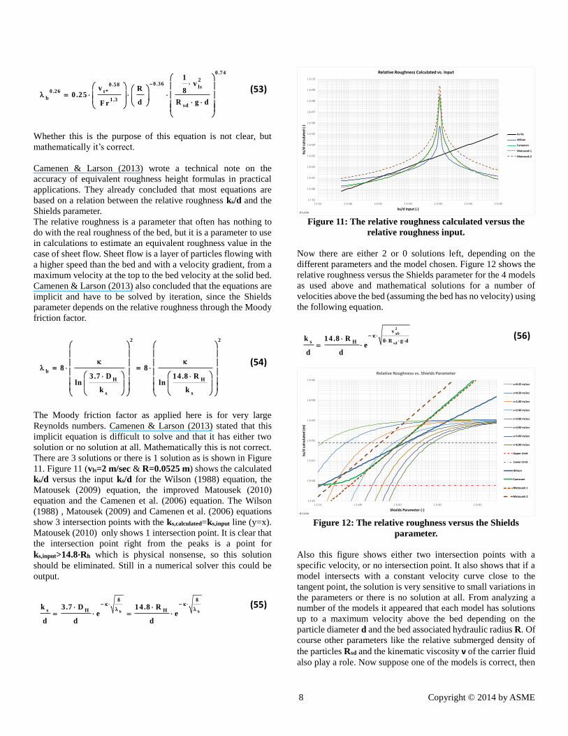
solution or no solution at all. Mathematically this is not correct.

There are 3 solutions or there is 1 solution as is shown in Figure

11. Figure 11 (vls=2 m/sec & R=0.0525 m) shows the calculated

ks/d versus the input ks/d for the Wilson (1988) equation, the

Matousek (2009) equation, the improved Matousek (2010)

equation and the Camenen et al. (2006) equation. The Wilson

(1988) , Matousek (2009) and Camenen et al. (2006) equations

show 3 intersection points with the ks,calculated=ks,input line (y=x).

Matousek (2010) only shows 1 intersection point. It is clear that

the intersection point right from the peaks is a point for

ks,input>14.8·Rh which is physical nonsense, so this solution

should be eliminated. Still in a numerical solver this could be

output.

b b

8 8

s H Hk 3.7 D 14.8 R

e ed d d

(55)

Figure 11: The relative roughness calculated versus the

relative roughness input.

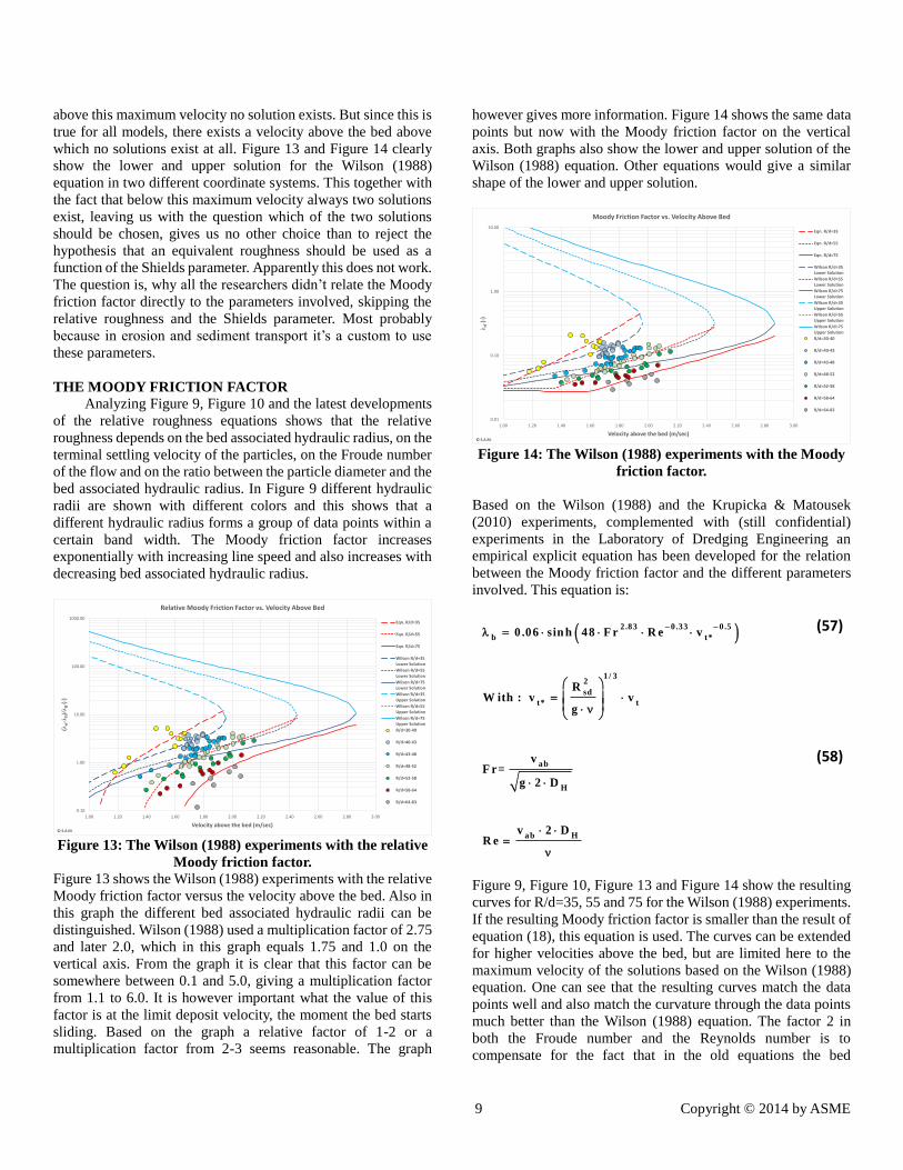
Now there are either 2 or 0 solutions left, depending on the

different parameters and the model chosen. Figure 12 shows the

relative roughness versus the Shields parameter for the 4 models

as used above and mathematical solutions for a number of

velocities above the bed (assuming the bed has no velocity) using

the following equation.

2

ab

sd

v

R g ds Hk 14 .8 R

ed d

(56)

Figure 12: The relative roughness versus the Shields

parameter.

Also this figure shows either two intersection points with a

specific velocity, or no intersection point. It also shows that if a

model intersects with a constant velocity curve close to the

tangent point, the solution is very sensitive to small variations in

the parameters or there is no solution at all. From analyzing a

number of the models it appeared that each model has solutions

up to a maximum velocity above the bed depending on the

particle diameter d and the bed associated hydraulic radius R. Of

course other parameters like the relative submerged density of

the particles Rsd and the kinematic viscosity ν of the carrier fluid

also play a role. Now suppose one of the models is correct, then

1.E-01

1.E+00

1.E+01

1.E+02

1.E+03

1.E+04

1.E+05

1.E+06

1.E+07

1.E+08

1.E+09

1.E+10

1.E-01 1.E+00 1.E+01 1.E+02 1.E+03 1.E+04 1.E+05

ks/d

cal

cula

ted

(-)

ks/d input (-)

Relative Roughness Calculated vs. Input

ks=ks

Wilson

Camenen

Matousek 1

Matousek 2

© S.A.M.

1.E-01

1.E+00

1.E+01

1.E+02

1.E+03

1.E+04

1.E+05

1.E-01 1.E+00 1.E+01 1.E+02 1.E+03

ks/d

cal

cula

ted

(m

)

Shields Parameter (-)

Relative Roughness vs. Shields Parameter

v=0.25 m/sec

v=0.50 m/sec

v=1.00 m/sec

v=2.00 m/sec

v=3.00 m/sec

v=4.00 m/sec

v=5.00 m/sec

v=6.00 m/sec

Upper Limit

Lower Limit

Wilson

Camenen

Matousek 1

Matousek 2

© S.A.M.

9 Copyright © 2014 by ASME

above this maximum velocity no solution exists. But since this is

true for all models, there exists a velocity above the bed above

which no solutions exist at all. Figure 13 and Figure 14 clearly

show the lower and upper solution for the Wilson (1988)

equation in two different coordinate systems. This together with

the fact that below this maximum velocity always two solutions

exist, leaving us with the question which of the two solutions

should be chosen, gives us no other choice than to reject the

hypothesis that an equivalent roughness should be used as a

function of the Shields parameter. Apparently this does not work.

The question is, why all the researchers didn’t relate the Moody

friction factor directly to the parameters involved, skipping the

relative roughness and the Shields parameter. Most probably

because in erosion and sediment transport it’s a custom to use

these parameters.

THE MOODY FRICTION FACTOR

Analyzing Figure 9, Figure 10 and the latest developments

of the relative roughness equations shows that the relative

roughness depends on the bed associated hydraulic radius, on the

terminal settling velocity of the particles, on the Froude number

of the flow and on the ratio between the particle diameter and the

bed associated hydraulic radius. In Figure 9 different hydraulic

radii are shown with different colors and this shows that a

different hydraulic radius forms a group of data points within a

certain band width. The Moody friction factor increases

exponentially with increasing line speed and also increases with

decreasing bed associated hydraulic radius.

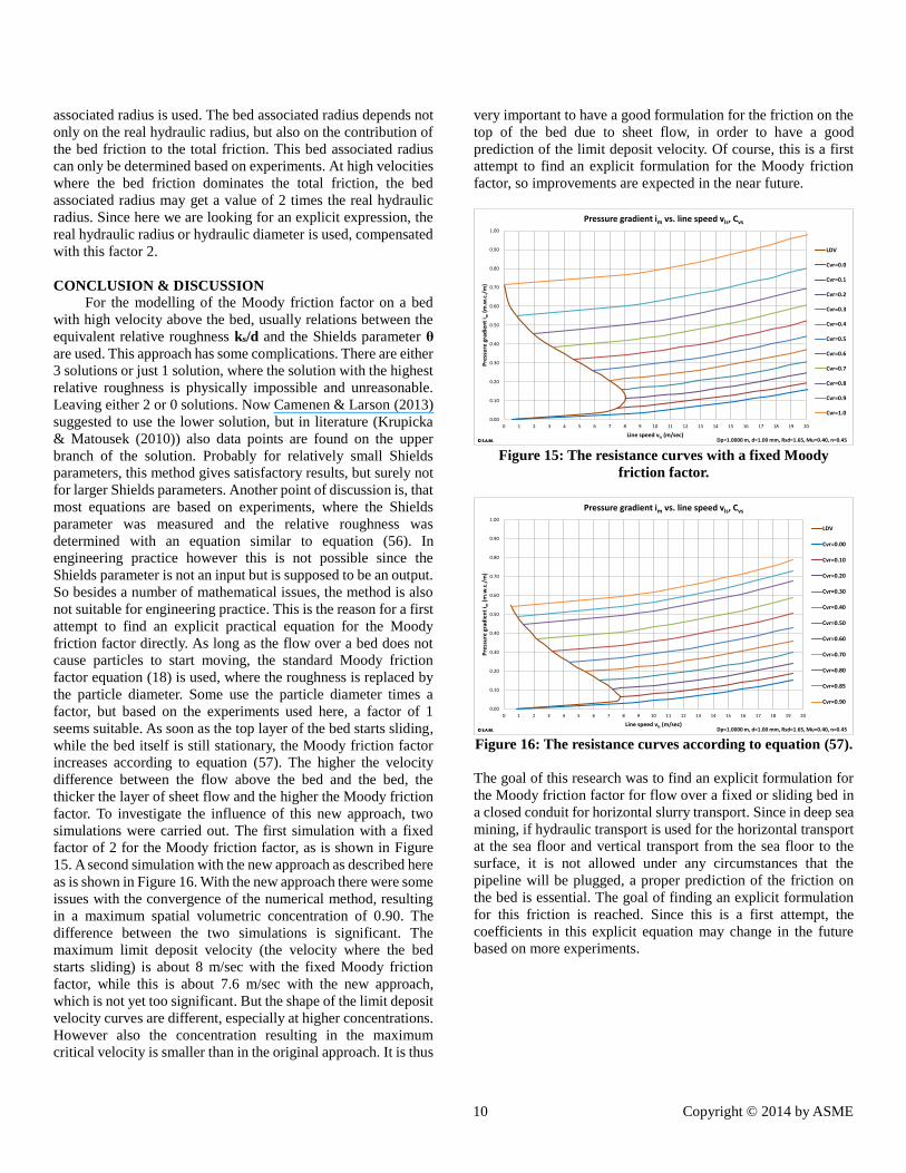
Figure 13: The Wilson (1988) experiments with the relative

Moody friction factor.

Figure 13 shows the Wilson (1988) experiments with the relative

Moody friction factor versus the velocity above the bed. Also in

this graph the different bed associated hydraulic radii can be

distinguished. Wilson (1988) used a multiplication factor of 2.75

and later 2.0, which in this graph equals 1.75 and 1.0 on the

vertical axis. From the graph it is clear that this factor can be

somewhere between 0.1 and 5.0, giving a multiplication factor

from 1.1 to 6.0. It is however important what the value of this

factor is at the limit deposit velocity, the moment the bed starts

sliding. Based on the graph a relative factor of 1-2 or a

multiplication factor from 2-3 seems reasonable. The graph

however gives more information. Figure 14 shows the same data

points but now with the Moody friction factor on the vertical

axis. Both graphs also show the lower and upper solution of the

Wilson (1988) equation. Other equations would give a similar

shape of the lower and upper solution.

Figure 14: The Wilson (1988) experiments with the Moody

friction factor.

Based on the Wilson (1988) and the Krupicka & Matousek

(2010) experiments, complemented with (still confidential)

experiments in the Laboratory of Dredging Engineering an

empirical explicit equation has been developed for the relation

between the Moody friction factor and the different parameters

involved. This equation is:

2.83 0 .33 0 .5

b t*0 .06 sin h 48 F r R e v

(57)

1 / 3

2

sd

t* t

ab

H

ab H

RW ith : v v

g

vF r=

g 2 D

v 2 DR e

(58)

Figure 9, Figure 10, Figure 13 and Figure 14 show the resulting

curves for R/d=35, 55 and 75 for the Wilson (1988) experiments.

If the resulting Moody friction factor is smaller than the result of

equation (18), this equation is used. The curves can be extended

for higher velocities above the bed, but are limited here to the

maximum velocity of the solutions based on the Wilson (1988)

equation. One can see that the resulting curves match the data

points well and also match the curvature through the data points

much better than the Wilson (1988) equation. The factor 2 in

both the Froude number and the Reynolds number is to

compensate for the fact that in the old equations the bed

0.10

1.00

10.00

100.00

1000.00

1.00 1.20 1.40 1.60 1.80 2.00 2.20 2.40 2.60 2.80 3.00

(λsf-λ

fl)/λ

fl(-

)

Velocity above the bed (m/sec)

Relative Moody Friction Factor vs. Velocity Above Bed

Eqn. R/d=35

Eqn. R/d=55

Eqn. R/d=75

Wilson R/d=35Lower Solution

Wilson R/d=55Lower Solution

Wilson R/d=75Lower Solution

Wilson R/d=35Upper Solution

Wilson R/d=55Upper Solution

Wilson R/d=75Upper Solution

R/d=30-40

R/d=40-43

R/d=43-48

R/d=48-52

R/d=52-58

R/d=58-64

R/d=64-83

© S.A.M.

0.01

0.10

1.00

10.00

1.00 1.20 1.40 1.60 1.80 2.00 2.20 2.40 2.60 2.80 3.00

λsf

(-)

Velocity above the bed (m/sec)

Moody Friction Factor vs. Velocity Above Bed

Eqn. R/d=35

Eqn. R/d=55

Eqn. R/d=75

Wilson R/d=35Lower Solution

Wilson R/d=55Lower Solution

Wilson R/d=75Lower Solution

Wilson R/d=35Upper Solution

Wilson R/d=55Upper Solution

Wilson R/d=75Upper Solution

R/d=30-40

R/d=40-43

R/d=43-48

R/d=48-52

R/d=52-58

R/d=58-64

R/d=64-83

© S.A.M.

10 Copyright © 2014 by ASME

associated radius is used. The bed associated radius depends not

only on the real hydraulic radius, but also on the contribution of

the bed friction to the total friction. This bed associated radius

can only be determined based on experiments. At high velocities

where the bed friction dominates the total friction, the bed

associated radius may get a value of 2 times the real hydraulic

radius. Since here we are looking for an explicit expression, the

real hydraulic radius or hydraulic diameter is used, compensated

with this factor 2.

CONCLUSION & DISCUSSION

For the modelling of the Moody friction factor on a bed

with high velocity above the bed, usually relations between the

equivalent relative roughness ks/d and the Shields parameter θ

are used. This approach has some complications. There are either

3 solutions or just 1 solution, where the solution with the highest

relative roughness is physically impossible and unreasonable.

Leaving either 2 or 0 solutions. Now Camenen & Larson (2013)

suggested to use the lower solution, but in literature (Krupicka

& Matousek (2010)) also data points are found on the upper

branch of the solution. Probably for relatively small Shields

parameters, this method gives satisfactory results, but surely not

for larger Shields parameters. Another point of discussion is, that

most equations are based on experiments, where the Shields

parameter was measured and the relative roughness was

determined with an equation similar to equation (56). In

engineering practice however this is not possible since the

Shields parameter is not an input but is supposed to be an output.

So besides a number of mathematical issues, the method is also

not suitable for engineering practice. This is the reason for a first

attempt to find an explicit practical equation for the Moody

friction factor directly. As long as the flow over a bed does not

cause particles to start moving, the standard Moody friction

factor equation (18) is used, where the roughness is replaced by

the particle diameter. Some use the particle diameter times a

factor, but based on the experiments used here, a factor of 1

seems suitable. As soon as the top layer of the bed starts sliding,

while the bed itself is still stationary, the Moody friction factor

increases according to equation (57). The higher the velocity

difference between the flow above the bed and the bed, the

thicker the layer of sheet flow and the higher the Moody friction

factor. To investigate the influence of this new approach, two

simulations were carried out. The first simulation with a fixed

factor of 2 for the Moody friction factor, as is shown in Figure

15. A second simulation with the new approach as described here

as is shown in Figure 16. With the new approach there were some

issues with the convergence of the numerical method, resulting

in a maximum spatial volumetric concentration of 0.90. The

difference between the two simulations is significant. The

maximum limit deposit velocity (the velocity where the bed

starts sliding) is about 8 m/sec with the fixed Moody friction

factor, while this is about 7.6 m/sec with the new approach,

which is not yet too significant. But the shape of the limit deposit

velocity curves are different, especially at higher concentrations.

However also the concentration resulting in the maximum

critical velocity is smaller than in the original approach. It is thus

very important to have a good formulation for the friction on the

top of the bed due to sheet flow, in order to have a good

prediction of the limit deposit velocity. Of course, this is a first

attempt to find an explicit formulation for the Moody friction

factor, so improvements are expected in the near future.

Figure 15: The resistance curves with a fixed Moody

friction factor.

Figure 16: The resistance curves according to equation (57).

The goal of this research was to find an explicit formulation for

the Moody friction factor for flow over a fixed or sliding bed in

a closed conduit for horizontal slurry transport. Since in deep sea

mining, if hydraulic transport is used for the horizontal transport

at the sea floor and vertical transport from the sea floor to the

surface, it is not allowed under any circumstances that the

pipeline will be plugged, a proper prediction of the friction on

the bed is essential. The goal of finding an explicit formulation

for this friction is reached. Since this is a first attempt, the

coefficients in this explicit equation may change in the future

based on more experiments.

0.00

0.10

0.20

0.30

0.40

0.50

0.60

0.70

0.80

0.90

1.00

0 1 2 3 4 5 6 7 8 9 10 11 12 13 14 15 16 17 18 19 20

Pre

ssu

re g

rad

ien

t i m

(m.w

.c./

m)

Line speed vls (m/sec)

Pressure gradient im vs. line speed vls, Cvs

LDV

Cvr=0.0

Cvr=0.1

Cvr=0.2

Cvr=0.3

Cvr=0.4

Cvr=0.5

Cvr=0.6

Cvr=0.7

Cvr=0.8

Cvr=0.9

Cvr=1.0

© S.A.M.© S.A.M.© S.A.M. Dp=1.0000 m, d=1.00 mm, Rsd=1.65, Mu=0.40, n=0.45

0.00

0.10

0.20

0.30

0.40

0.50

0.60

0.70

0.80

0.90

1.00

0 1 2 3 4 5 6 7 8 9 10 11 12 13 14 15 16 17 18 19 20

Pre

ssu

re g

rad

ien

t i m

(m.w

.c./

m)

Line speed vls (m/sec)

Pressure gradient im vs. line speed vls, Cvs

LDV

Cvr=0.00

Cvr=0.10

Cvr=0.20

Cvr=0.30

Cvr=0.40

Cvr=0.50

Cvr=0.60

Cvr=0.70

Cvr=0.80

Cvr=0.85

Cvr=0.90

© S.A.M.© S.A.M.© S.A.M. Dp=1.0000 m, d=1.00 mm, Rsd=1.65, Mu=0.40, n=0.45

11 Copyright © 2014 by ASME

NOMENCLATURE Ap Cross section pipe m2

A1 Cross section above bed m2

A2 Cross section bed m2

Cvb Volumetric bed concentration -

d Particle diameter m DH Hydraulic diameter m

Dp Pipe diameter m

F Force kN

F1,fl Force between fluid and pipe wall kN

F12,fl Force between fluid and bed kN

F2,pr Force on bed due to pressure kN

F2,fr Force on bed due to friction kN

F2,fl Force on bed due to pore fluid kN

FN Normal force kN

FW Weight of bed kN

Ffr Friction force kN Fr Froude number -

g Gravitational constant 9.81 m/sec2

im Pressure gradient mixture -

iplug Pressure gradient plug flow -

ks Bed roughness m

L Length of pipe m

Op Circumference pipe m

O1 Circumference pipe above bed m

O2 Circumference pipe in bed m

O12 Width of bed m

p Pressure kPa Re Reynolds number -

Rsd Relative submerged density -

R Bed associated radius m

RH Hydraulic radius m

u* Friction velocity m/sec

v Velocity m/sec

vab Velocity above the bed m/sec vt Terminal settling velocity m/sec

vt* Dimensionless terminal settling velocity -

vls Line speed m/sec

v1 Velocity above bed m/sec

v2 Velocity bed m/sec

β Bed angle rad

ε Pipe wall roughness m

ρfl Density carrier fluid ton/m3

θ Shields parameter -

θc Critical Shields parameter -

λ Moody friction factor -

λfl Moody friction factor fluid-pipe wall -

λb Moody friction factor on the bed -

λ1 Moody friction factor with pipe wall -

λ2 Moody friction factor with pipe wall -

λ12 Moody friction factor on the bed -

ν Kinematic viscosity m2/sec

τ Shear stress kPa

τfl Shear stress fluid-pipe wall kPa

τ1,fl Shear stress fluid-pipe above bed kPa

τ12,fl Shear stress bed-fluid kPa

τ2,fl Shear stress fluid-pipe in bed kPa

τ2,fr Shear stress from sliding friction kPa

μfr Sliding friction coefficient -

σn Normal stress kPa

12 Copyright © 2014 by ASME

REFERENCES Camenen, B., & Larson, M. (2013). Accuracy of Equivalent

Roughness Height Formulas in Practical Applications.

Journal of Hydraulic Engineering., 331-335. Camenen, B., Bayram, A. M., & Larson, M. (2006). Equivalent

roughness height for plane bed under steady flow.

Journal of Hydraulic Engineering, 1146-1158.

Grant, W. D., & Madsen, O. S. (1982). Movable bed roughness

in unsteady oscillatory flow. Journal Geophysics

Resources, 469-481.

Madsen, O. S., Wright, L. D., Boon, J. D., & Chrisholm, T. A.

(1993). Wind stress, bed roughness and sediment

suspension on the inner shelf during an extreme storm

event. Continental Shelf Research 13, 1303Ð1324. .

Matousek, V., & Krupicka, J. (2009). On equivalent roughness

of mobile bed at high shear stress. Journal of Hydrology

& Hydromechanics, Vol. 57-3., 191-199.

Matousek, V., & Krupicka, J. (2010). Semi empirical formulae

for upper plane bed friction. Hydrotransport 18 (pp. 95-

103). BHRA.

Miedema, S. A. (2014). AN ANALYSIS OF SLURRY

TRANSPORT AT LOW LINE SPEEDS. ASME 2014

33rd International Conference on Ocean, Offshore and

Arctic Engineering, OMAE. (p. 11). San Francisco,

USA.: ASME.

Miedema, S. A., & Ramsdell, R. C. (2013). A Head Loss Model

for Slurry Transport based on Energy Considerations.

World Dredging Conference XX (p. 14). Brussels,

Belgium.: WODA.

Miedema, S. A., & Ramsdell, R. C. (2014). An Analysis of the

Hydrostatic Approach of Wilson for the Friction of a

Sliding Bed. WEDA/TAMU (p. 21). Toronto, Canada:

WEDA.

Nielsen, P. (1981). Dynamics and geometry of wave generated

ripples. Journal of Geophysics Research, Vol. 86.,

6467-6472.

Ramsdell, R. C., & Miedema, S. A. (2013). AN OVERVIEW OF

FLOW REGIMES DESCRIBING SLURRY

TRANSPORT. WODCON XX (p. 15). Brussels,

Belgium.: WODA.

Rijn, L. v. (1993). Principles of Sediment Transport, Part 1. .

Blokzijl: Aqua Publications.

Talmon, A. (2013). Analytical model for pipe wall friction of

pseudo homogeneous sand slurries. Particulate Science

& technology: An International Journal, 264-270.

Televantos, Y., Shook, C. A., Carleton, A., & Street, M. (1979).

Flow of slurries of coarse particles at high solids

concentrations. Canadian Journal of Chemical

Engineering, Vol. 57., 255-262.

Wikramanayake, P. N., & Madsen, O. S. (1991). Calculation of

movable bed friction factors. Vicksburg, Mississippi.:

Tech. Rep. DACW-39-88-K-0047, 105 pp., Coastal

Eng. Res. Cent.,.

Wilson, K. C. (1988). Evaluation of interfacial friction for

pipeline transport models. Hydrotransport 11 (p. B4).

BHRA.

Wilson, K. C., Addie, G. R., & Clift, R. (1992). Slurry Transport

using Centrifugal Pumps. New York: Elsevier Applied

Sciences.