AIAA-2006-0623-Internal Flow Noise

Internal Flow and Noise of Chevrons and Lobe Mixers in Mixed-Flow Nozzles

Vinod G. Mengle*

The Boeing Company, Seattle, WA, 98124-2207

Lobe mixers have been traditionally used in mixed-flow exhaust nozzles of turbofan engines to enhance mixing in order to increase thrust efficiency and reduce noise. Earlier, the author has shown how the use of internal chevrons, instead of lobe mixers, in combination with external chevrons on the mixed-nozzle lip can reduce the far field perceived noise level below that of lobe mixers for a range of typical gas conditions at take-off. In this paper, we explore experimentally the mean flow-field characteristics of internal chevrons inside the hot nozzle by developing a unique nozzle with a set of rotatable internal rakes. The inner boundary layer profile at the nozzle exit plane is also obtained and can be useful in designing immersions of external chevrons. A lower bound on the noise contribution of this internal mixing to far field noise is then found by using the technique of hard- and soft-walled nozzles. Similar internal flow and internal noise characteristics are then found for an advanced lobe mixer, as well as a simple splitter nozzle. The “gentle” mixing due to internal chevrons appears to correlate with lower contribution of internal jet noise to far field. However, the simple splitter nozzle has a fairly strong contribution from internal jet noise. Besides giving an improved understanding of these flows and noise characteristics, the experimental database generated can be used to validate predictive theories for internal flow and internal jet noise.

I. Introduction N mixed-flow nozzles (or, internally-mixed nozzles) of modern turbofan engines, where the hot core flow and fan flow are mixed inside a nozzle duct, the traditional device for reducing jet noise in a thrust-efficient manner (in

comparison to a simple splitter) has been the lobe mixer. However, recently the author has shown1 for the first time that appropriately designed combinations of "internal" chevrons, in lieu of lobe mixers, and "external" chevrons added to the aft mixed nozzle lip can reduce jet noise as much as, or even better than, the quietest lobe mixers for typical high bypass ratio nozzles at take-off conditions, when compared at same thrust-level and nozzle size. Internal chevrons, by themselves, as illustrated in Fig. 1(a), also proved to be quieter than simple round splitter nozzles.

I

Internal chevrons reduced low frequency noise below that of simple splitter with hardly any high frequency “lift.” External chevrons further aided the internal chevrons by reducing the low frequency noise even more. Lobe mixers, on the other hand, reduce the low frequency noise tremendously to compensate for their high frequency lift, if any. Thus there appears to be a paradigm shift in the way overall perceived noise level can be reduced for internally mixed nozzles: rather than reducing the low frequency noise tremendously and accepting high frequency lift, as with lobe mixers, one can reduce the low frequency noise somewhat less but without much high frequency lift by using appropriately designed chevrons.

Two key reasons were suggested for this beneficial behavior of internal chevrons in mixed-flow nozzles. To understand them note that in such internally mixed nozzles, the noise generated inside the nozzle (termed “internal” jet noise) due to the turbulent mixing between the core and the fan stream, downstream of the mixer, can also contribute to the far field noise in addition to the classic jet mixing noise generated outside the nozzle (termed “external’ jet noise). Figure 1(b) illustrates these two sources of jet noise. Then the reasons suggested for their success were: the "gentler" mixing of chevrons which supposedly reduces the contribution of internal jet mixing noise and, secondly, the higher discharge coefficient of chevrons compared to lobe mixers (the latter typically have higher blockage area ratio due to the several convoluted lobes).

Although the discharge coefficients were measured and compared earlier for such internal chevrons and lobe mixers, their internal flow and internal noise characteristics were not verified. Internal flow evolution, in general, * Engineer/Scientist, Acoustics and Fluid Mechanics, P.O. Box 3707, MC: 67-ML, Senior AIAA Member

American Institute of Aeronautics and Astronautics

1

44th AIAA Aerospace Sciences Meeting and Exhibit9 - 12 January 2006, Reno, Nevada

AIAA 2006-623

Copyright © 2006 by The Boeing Company. Published by the American Institute of Aeronautics and Astronautics, Inc., with permission.

has not been reported in the published literature for such nozzles, primarily because of the difficulty of measuring these quantities deep inside the mixing duct without interference or without any possible optical means for non-transparent nozzles. Additionally, the internal boundary layer thickness at the mixed-nozzle lip, which is also an important parameter for determining the so-called "immersion" of external chevrons has also not been studied earlier. In this paper, we present for the first time (i) the axial evolution of the mean flow properties inside such nozzles using a unique apparatus, (ii) the internal boundary layer profiles at the nozzle exit plane, and (iii) their internal mixing noise contribution in the far field using diagnostic techniques previously developed by the author2. We also compare and contrast these three quantities for internal chevrons, lobe mixers and simple splitter. This gives a more complete understanding of the flow and noise processes that take place inside these nozzles and would help in even further reduction of jet noise as well as provide a database for validation of flow and noise prediction methods.

The enhanced internal mixing in such devices is produced by the axial vorticity generated by the lobe mixers or internal chevrons. The typical width of these mixing devices, that is, the lobe width or the internal chevron width at the root, governs the maximum size of the typical axial vortices ("mushroom-shaped" vortex pairs) in the cross-plane, and provides an additional length-scale for mixing and, hence, for the frequency-scaling of internal mixing noise. The lobe widths or the chevron spans, being smaller than the nozzle diameter, provide higher frequency-scaling for the internal noise than that from external noise, which is known to scale with the nozzle exit diameter. Such moderate-to-high frequency internal sound has more annoyance (or, noy) weighting than lower frequency external sound, and can raise the perceived noise levels for these mixers – the internal noise from lobe mixers, for example, can give a second hump in their far field spectral noise characteristics3. Hence, it is crucial to understand these noise characteristics, especially, for the newer internal chevrons and relate it to the corresponding internal flow properties.

This paper presents one part of a comprehensive series of tests that was conducted by the author in Boeing's Low Speed Aeroacoustic Facility (LSAF) for such internally mixed nozzles with chevrons and lobe mixers in 2003. Other relevant material can be found in Refs. 1, 2 and 4. The focus here is on internal chevrons and the comparative results for lobe mixers and simple splitter are given more for a complete exposition.

The paper is divided into two parts: (a) internal flow, and (b) internal noise. We begin by presenting the unique nozzle instrumentation that was developed to measure the internal flow, and also briefly describe the internal jet noise diagnostics using the soft-wall/hard-wall technique. We limit ourselves to obtaining only the gross mean flow characteristics inside the nozzle. Then the experimental results for each part are presented separately and discussed.

II. Nozzle Models and Instrumentation The test was carried out on the high temperature jet simulator in Boeing’s LSAF. The LSAF is basically a low

speed open jet wind-tunnel located in a large anechoic chamber. Other details of this facility can be found in Ref. 1. The scaled nozzle models, described below, were mounted in the dual-flow hot jet rig and for the purposes of this test the open jet wind-tunnel flow was not used. A horizontal polar array of microphones at a radius of R = 25 ft from the nozzle exit plane center and spanning the directivity angles (measured from the jet inlet axis) from 45 degrees to 145 degrees was used to measure the far field sound. A. Mixer Scale Models

Although several internal chevrons and lobe mixers were tested using these techniques, results for only one internal chevron nozzle case and one lobe mixer case are presented here for brevity. Figure 2 shows the internal chevron mixer (IC2) and the lobe mixer (M3) whose results are presented: IC2 has 18 similar-shaped chevrons, which are triangular, and bent slightly inwards; M3 is a state-of the-art lobe mixer with 18 uniform unscalloped lobes. In addition, for the sake of comparison, internal noise results are also presented for the simple splitter (SS) or confluent nozzle which does not have any enhanced mixing devices.

The nozzle exit diameter, D, is 6.67 in. and the mixing length, L, (defined nominally as the distance between the mixer tip and the nozzle exit plane) is nominally 14.46 in. for IC2 mixer and 14.87 in. for M3 mixer. The mixing-length to exit diameter ratio, L/D, thus becomes 2.17 or 2.23 which is unusually long. More typical mixed-flow nozzles have L/D = 1 or so. This makes the process of probing the internal flow of such long nozzles even more difficult. B. Internal Flow Measurement

A good scalar marker for the axial evolution of the mean flow inside such turbofan nozzles at typical take-off operating conditions, where the core flow is hot and the fan flow is relatively cool, is the total temperature5. Other


2

scalar and vector markers to measure flow-mixedness have also been used in past CFD and experimental studies of internally mixed nozzles with lobe mixers by the MIT group6 and UTRC/Pratt & Whitney group7, but total temperature is the simplest measurable scalar. Yu et al8 have also measured detailed mean cross-stream velocities for lobe mixers kept in transparent rectangular ducts using optical or laser diagnostic tools, such as, laser-Doppler anemometry, and, hence, computed the evolution of mean axial vorticity and circulation for lobe mixers. However, for practical metallic scaled nozzles which are opaque, such as those used in our experiments with hot flows, the use of optical means for internal flows is rendered impossible.

To gain a reasonable understanding of such internal flows one needs a snap-shot of these flow values in the whole cross-section, or at least in one azimuthal period of the mixer, if it is periodic, and repeated at different axial stations in order to understand its axial evolution. Hence, even though measurement of turbulent flow properties, such as, turbulent velocity components may not be impossible at each point with, say, a hot-wire anemometer or the like, it would be extremely cumbersome for points deep inside the nozzle across several cross-planes in a hot flow environment. Hence, in this study where the goal was only to get a global understanding of the internal flow differences between internal chevrons and lobe mixers, and its relation to internal noise, we limited ourselves to measuring only the mean total temperature (TT) across one-full period of the mixers at several axial stations. In addition, we also used wall static pressure taps, a boundary layer probe at the nozzle exit, and a wake rake in the plume.

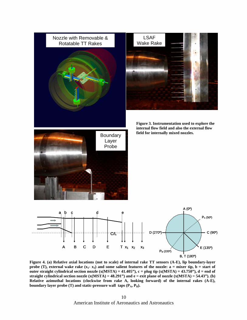
Figure 3(a) shows the inside view (a CAD/CAM view) of the unique total temperature rakes that were built for measurements inside the nozzle. The convergent nozzle itself was made up of three different pieces – two straight cylinders, just aft of the mixer exit plane, and an aft-most conical piece for the convergent nozzle, as seen in Fig. 1(a). The TT-rakes were designed to be placed at maximum five axial stations, each at a different azimuthal location to avoid interference, with two rakes per straight cylindrical portion of the nozzle and one rake in the conical portion. Each rake, placed radially, is of increasing length as we go downstream, to avoid interference near the central axis portion, especially, for the downstream rakes, and has varying number of sheathed thermocouples with varying distances between them. These rakes were removable and could be used one at a time, to avoid interference, or as many as five at a time, if required. The choice of using only one rake at a time at different axial locations to avoid any rake-to-rake interference was deemed to be too laborious, especially, when the mixing length is very long.

Since these rakes were fixed to the nozzle, the azimuthal direction could be traversed simultaneously at multiple axial stations by rotating the aft portion of the whole nozzle with respect to the mixer. To avoid leakage but allow rotation of the nozzle, two degrees at a time, the external instrumented nozzle was removed and reattached to the upstream flange every time a radial survey was made at a different azimuthal angle. An indexing ring fixture was made on the nozzle flange upstream to keep tab on the clocking values (angle = θ from some fixed reference) as the nozzle was rotated. Thus, for example, if there are 18 periodic internal chevrons or lobes then the azimuthal period is 20 degrees, and these rakes needed positioning at 11 different angles to cover one period from end to end. Each rake will cover a different azimuthal sector when the nozzle is rotated, as can be seen from Fig. 4(b), but assuming periodicity in the flow for periodic mixers, we can approximately consider the flow in each sector as an axial progression of the flow in a lobe period. This process is fairly arduous especially when the flows are hot and cooling time is needed each time the nozzle is rotated manually; however, it gives an accurate assessment of the evolution of the internal flow.

Figure 4(a) shows the axial locations of the rakes, named, A, B, C, D and E, in relation to the salient features of the nozzle, and Fig. 4(b) shows their azimuthal locations relative to rake A. The absolute values of their axial locations, in terms of the model station, x(MSTA), referred to some fixed station on the nozzle model far upstream are given in Table 1, where their locations in terms of percentage of the mixing lengths (defined here as the distance between the mixer tip plane and the nozzle exit plane) for the two different mixers (IC2 and M3) are also noted. Thus note that the two most upstream rakes, A and B, are located diametrically opposite to reduce mutual rake-to-rake interference, and so are the next two rakes C and D, although the latter are orthogonal to the first pair. The most downstream rake, E, is located azimuthally exactly between C and B, again to avoid rake interference, if used in conjunction with others. The blockage area ratio of these rakes, with multiple thermocouples, was minimized by using standard streamlined struts; the nominal blockage area ratio varied from as low as 1.2% for A to 1.99% for E.

There were also two axial arrays of static pressure taps on the nozzle wall, PA and PB, downstream of the mixer exit plane. Their azimuthal locations are given in Fig. 4(b) and are designed to coincide with the chevron tip (or lobe valley) and the chevron root (or lobe crown), respectively, for the mixers with 18 periods. These static pressure arrays, being fixed to the nozzle, of course rotate when the nozzle is rotated; thus, they can give the azimuthal flow properties on the inner nozzle wall.

Figure 3 also shows the relative location of the boundary layer probe, which is a hypodermic needle, flattened to an ellipse at its tip (with major axis parallel to the wall), to measure total pressure. It was designed to traverse the


3

radial direction in minute increments (as low as 0.005 in.) near the nozzle exit plane using an outside traversing mechanism stationed at 6 o'clock position (see Fig. 4(b)). Hence, although the nozzle is kept inside a free-jet wind-tunnel to simulate flight effects, the boundary-layer probe could be used only under static wind-tunnel conditions.

Figure 3 further shows the LSAF wake rake that was used to measure total temperature (TT), total pressure (PT) and also static pressure (Ps) in the external plume. The total temperature thermocouples and total/static pressure probes are placed alternately half-an-inch apart radially (short and long supports, respectively, in the photo) to avoid mutual interference, and were limited for use in subsonic flow conditions. This LSAF wake rake can traverse in three orthogonal directions and can give cross-sectional mean flow information at various axial stations downstream of the nozzle exit plane. Since the total temperature sensor is axially offset from the total pressure probe by 2.875 in., it would require two passes of this rake to cover a given axial station in order to find TT, PT and Ps at that station. Brief data was obtained at three axial stations, x1, x2 and x3, using this wake rake, and is shown in Fig. 4(a). Only minimal use is made of the external flow data from this wake rake in this paper, as the focus here is more on the internal flow characteristics.

C. Internal Jet Noise Measurement

The complementary part of this paper is the measurement of internal jet noise for such nozzles. Although in this study we used all the three methods developed by the author in Ref. 2, namely, (i) softwall/hardwall difference, (ii) modified shifted angle with varying free-jet speed, and (iii) cross-spectra between an internal kulite and two far-field microphones, only the results from the first method will be discussed in this paper. The first two methods gave corroborating results previously for lobe mixers and were deemed successful, but the last one did not.

In the softwall/hardwall method, as the name implies, the difference in far-field sound due to hardwall and softwall nozzles is attributed to internal noise. The softwall nozzle is a special nozzle with same internal flow lines as the hardwall but made with broadband lining and perforated inner wall. The softwall nozzle was proven earlier to reduce sound produced by internal speakers (also seen in fig. 3(a)) by a large magnitude beyond a certain frequency (5000 hz) in both the no-flow and with-flow situations. More details on this softwall attenuation calibration can be seen in Ref. 2. This method obviously has certain limitations, as described in Ref. 2, and gives a lower bound of the internal noise contribution in the far field at different directivity angles and frequencies under static wind-tunnel conditions. We will explore this lower bound on internal jet noise more fully in a later section.

Thus, in summary, we used three different pieces of external nozzle hardware which had the same internal flow lines but different external flow lines: the un-instrumented reference nozzle with smooth external contours, the instrumented nozzle with internal total temperature rakes and static pressure taps, and the softwall nozzle. The first nozzle can be used in free-jet simulation tests whereas, the latter two cannot. In this paper, we are mainly interested in the static tests, with wind-tunnel off, for understanding the internal flow and internal noise characteristics.

III. Experimental Results and Discussion Tests were conducted at several typical gas conditions representative of operating points at take-off of a modern

turbofan engine cycle, the same as used in Ref. 1. Table 2 shows these operating conditions in terms of the nozzle pressure ratios (total pressure at an upstream charging station to ambient pressure) and total temperatures in the primary (NPRP, TTP) and the secondary streams (NPRS, TTS). Only a subset of the total test points is shown which are representative of full take-off power although other gas conditions representative of cut-back conditions were also tested.

Since we will be comparing results from the 18-lobed internal chevron nozzle (IC2) and the 18-lobed mixer (M3) it is better to clock them similarly so that the radial flow characteristics will correspond to each other. Since the flow goes radially outwards in the valley between two flipped-in chevrons or near the crown of a lobe mixer, we placed IC2 with one of its valleys at top-dead center (TDC) and M3 with one of its lobe crowns at TDC.

A. Internal Flow We will focus on TO # 2 in this paper. Note that although NPRS is supercritical (>1.89), in internally mixed

nozzles it does not necessarily imply that the secondary flow speed is supersonic at the mixer exit plane because the static pressure there (upstream of the nozzle exit plane) need not have expanded to ambient pressure. The wall static pressure is a good indicator of the pressures in the flow and flow speeds near the wall.

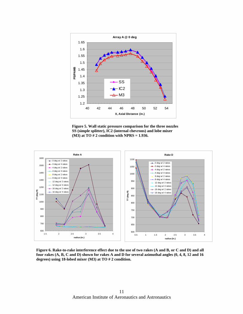
Figure 5 shows the wall static pressure, PS, normalized with the ambient pressure, PAMB, for all the three mixer nozzles (SS = Simple Splitter; IC2 = Internal Chevrons: M3 = 18-lobed mixer) on array A which is located at 50 deg. from the top dead center (see Fig. 4(b)). This coincides with a chevron tip or a lobe keel (valley). The general shape of these curves are similar for all these nozzles: initially rising, then almost constant and then quickly


4

decreasing. The rising portion is in the diverging area of the nozzle where the plug is located; the almost constant value corresponds to the constant area of the nozzle in the straight cylindrical portion; and, the decreasing values correspond to the convergent portion of the nozzle. These correspond to area-velocity relations from simple one-dimensional considerations for subsonic flows.

There is almost no difference between IC2 and SS which implies that the flow speeds near the nozzle wall must be similar and subsonic. Since the simple splitter (SS) nozzle is not expected to have great mixing between the two streams it must be the secondary flow that must be clinging to the wall throughout the mixing length. If, for IC2 nozzle, it is also the secondary flow that is still clinging to the wall, as seen from this pressure plot, then even though it may have enhanced the mixing between the two streams, the high-speed core flow has presumably not yet reached the wall. On the other hand, the lobe mixer, M3, shows slightly lower static pressures which implies that the flow speeds near the wall must be higher than for IC2 – which is possible if the high-speed core flow has already mixed with the low-speed fan stream and this partially mixed flow is flowing by the wall. We will see if this simple interpretation corroborates with the total temperature profiles seen by the internal TT-rakes.

Before we present the results for the internal TT-rakes it is pertinent to check first if multiple rakes can cause mutual rake-to-rake flow interference due to the downstream rake being in the wake of the upstream rake although we have already tried to minimize this interaction by keeping them at different azimuthal locations. The more the number of rakes to be used simultaneously, the quicker it is to take data at several axial stations simultaneously. For example, to cover same axial stations and azimuthal angles four rakes will take half the time for two rakes, and two rakes will take half the time for one rake. With data to be taken at several azimuthal angles and several axial stations, this does become an important time consideration.

Figure 6 shows an example of the difference in TT by using two rakes at a time (A and B, or C and D) to using all four of them simultaneously for the lobe mixer M3 which is expected to have the strongest mixing and, hence, most complex flow pattern. Note that A and B are diametrically opposite to each other (see Fig. 4(b)), and so are C and D, so that mutual interference between A and B itself (or C and D) is assumed to be minimal. The data is shown at several different nozzle clock-indexing angles (θ = 0, 4, 8, 12 and 16 degrees (see legend)) as the external nozzle is rotated (with the lobe mixer fixed) and the rakes scan different azimuthal angles of the lobe mixer flow. Interestingly, the most downstream rake D shows no difference in TT whether two or four rakes are used, implying minimal rake-to-rake interference (A/B to C/D). This is similar to the data for rakes C and B (not shown for brevity). However, Rake A, which although the most upstream, shows slight evidence of interference effects at θ = 16º and 4º but not at other angles. Although disturbances can travel upstream in subsonic flows, as this may be the case from the wall static pressure tap data, note that these two angles are closest to the side walls of the lobe mixer where the two flows are mixing strongly and the flow is unsteady. For this reason, to improve accuracy, we decided to use only two diametrically opposite rakes at a time (A and B, or C and D) but not all four; the most downstream rake E was used alone so that it is not in the wake of any upstream rakes.

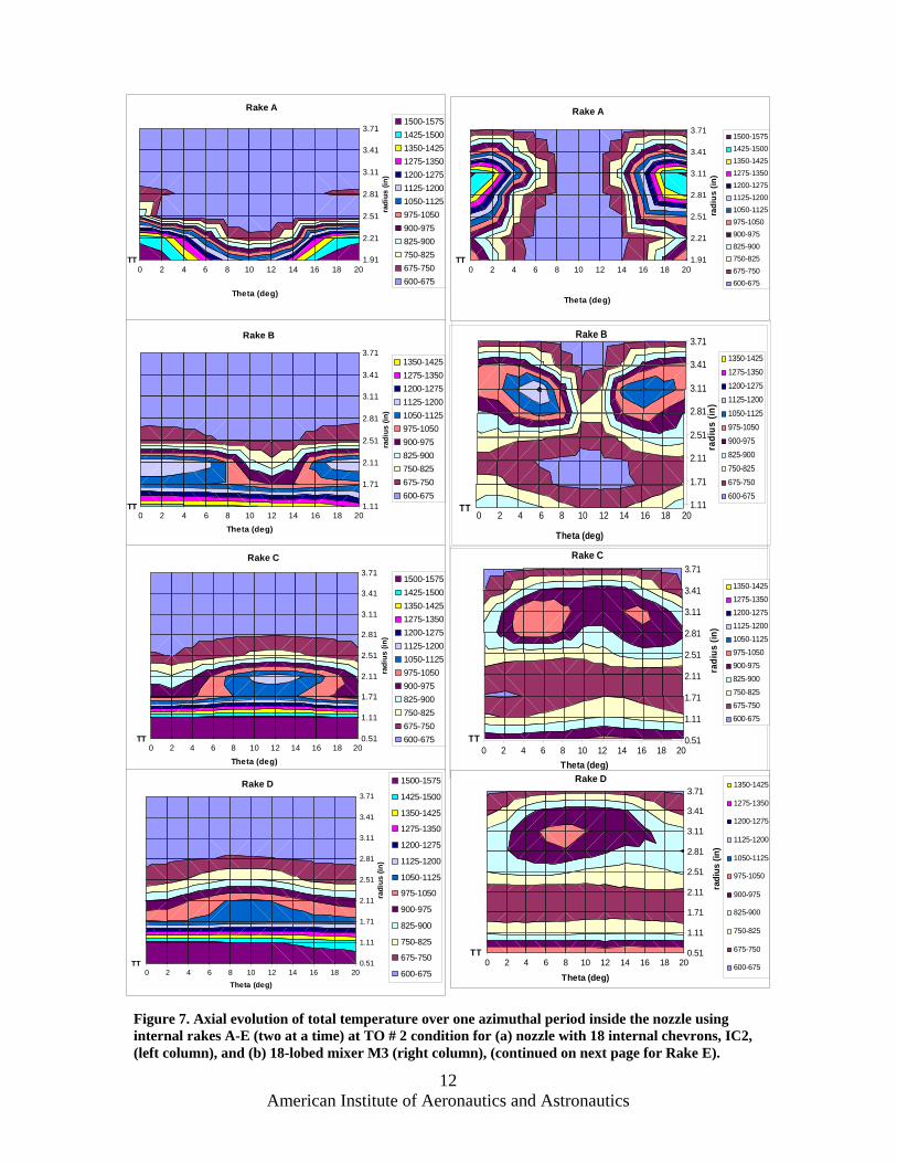
Now let us examine the internal flow total temperatures for the internal chevron nozzle, IC2, and the lobe mixer, M3, at different axial stations along their mixing length. Figure 7(a) shows these results for IC2 and 7(b) for M3. The pie sector of the spanned region for each rake is mapped to a rectangular region with (r, θ) as coordinates, where θ is the common nozzle indexing angle mentioned earlier. Thus, the region near the central axis (small values of r) appears to be considerably expanded compared to the region near the nozzle wall (larger values of r).

Another item to note when looking at these contour plots is that each rake is located at a different azimuthal angle (clocked differently) with respect to the chevrons, so that appropriate shift in angle needs to be accounted for when interpreting results relative to the location of the chevrons. Thus, for example, rakes A and B are originally located at the valleys between chevrons, so that θ = 0 or 20 for them corresponds to the chevron valleys (or lobe crowns); whereas, θ = 10 corresponds to the chevron tips (or lobe valleys). For Rakes C and D, θ = 0 or 20 in their plots correspond to chevron tips (or lobe valleys), whereas, θ = 10 corresponds to chevron valley (or lobe crowns). Hence, when comparing these plots from Rake C to Rake A we need to account for this shift of 10 deg. in Rake C. Similarly Rake E, originally located at 135 deg., is -5 deg. from the chevron tip (or lobe valley) and an appropriate shift of -5 deg. is needed when comparing plots from Rakes A and B.

Since the core flow is hotter than the fan flow, Fig. 7 immediately shows the smaller radially shift of the core flow in internal chevrons IC2 as compared to lobe mixer M3. Several previous CFD studies with lobe mixers have shown that the eye of the hot core flow can usually be associated with the eye of the streamwise vortex generated by such devices. Thus the radial and the azimuthal migration of the axial-vortex eyes is clearly captured in these plots, especially, for the lobe mixer. It also shows that in general at least the scalar mixing in internal chevrons is far less violent than in lobe mixers.


5

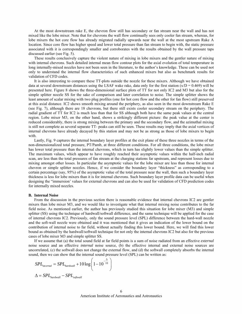
At the most downstream rake E, the chevron flow still has secondary or fan stream near the wall and has not mixed like the lobe mixer. Note that for chevrons the wall flow continually sees only cooler fan stream, whereas, for lobe mixers the hot core flow has already migrated radially upwards near the wall at the most upstream Rake A location. Since core flow has higher speed and lower total pressure than fan stream to begin with, the static pressure associated with it is correspondingly smaller and corroborates with the results obtained by the wall pressure taps discussed earlier (see Fig. 5).

These results conclusively capture the violent nature of mixing in lobe mixers and the gentler nature of mixing with internal chevrons. Such detailed internal mean flow contour plots for the axial evolution of total temperature in long internally-mixed nozzles have not been seen in the literature, to the author’s knowledge. These can be used not only to understand the internal flow characteristics of such enhanced mixers but also as benchmark results for validation of CFD codes.

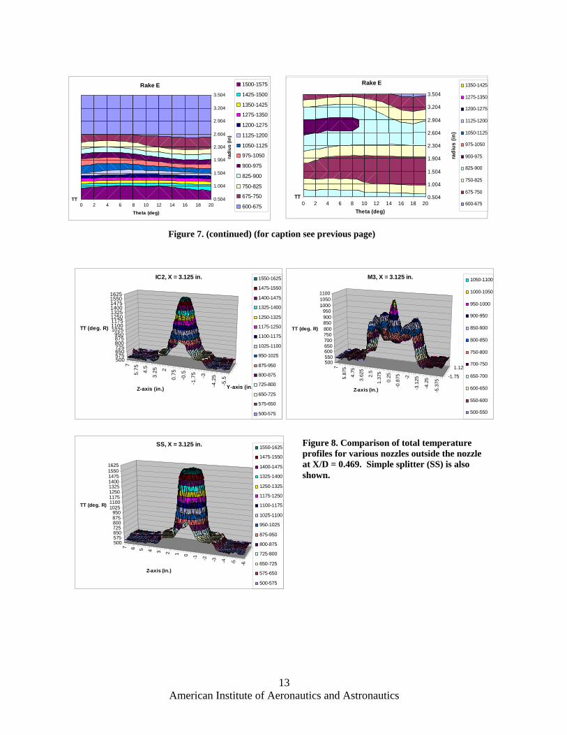
It is also interesting to compare these TT-plots outside the nozzle for these mixers. Although we have obtained data at several downstream distances using the LSAF wake rake, data only for the first station (x/D = 0.469) will be presented here. Figure 8 shows the three-dimensional surface plots of TT for not only IC2 and M3 but also for the simple splitter nozzle SS for the sake of comparison and later correlation to noise. The simple splitter shows the least amount of scalar mixing with two plug profiles (one for hot core flow and the other for fan flow) still preserved at this axial distance. IC2 shows smooth mixing around the periphery, as also seen in the most downstream Rake E (see Fig. 7), although there are 18 chevrons, but there still exists cooler secondary stream on the periphery. The radial gradient of TT for IC2 is much less than that for SS although both have the same peak values at the central region. Lobe mixer M3, on the other hand, shows a strikingly different picture: the peak value at the center is reduced considerably, there is strong mixing between the primary and the secondary flow, and the azimuthal mixing is still not complete as several separate TT- peaks can still be seen. These results may imply that the axial vortices of internal chevrons have already decayed by this station and may not be as strong as those of lobe mixers to begin with.

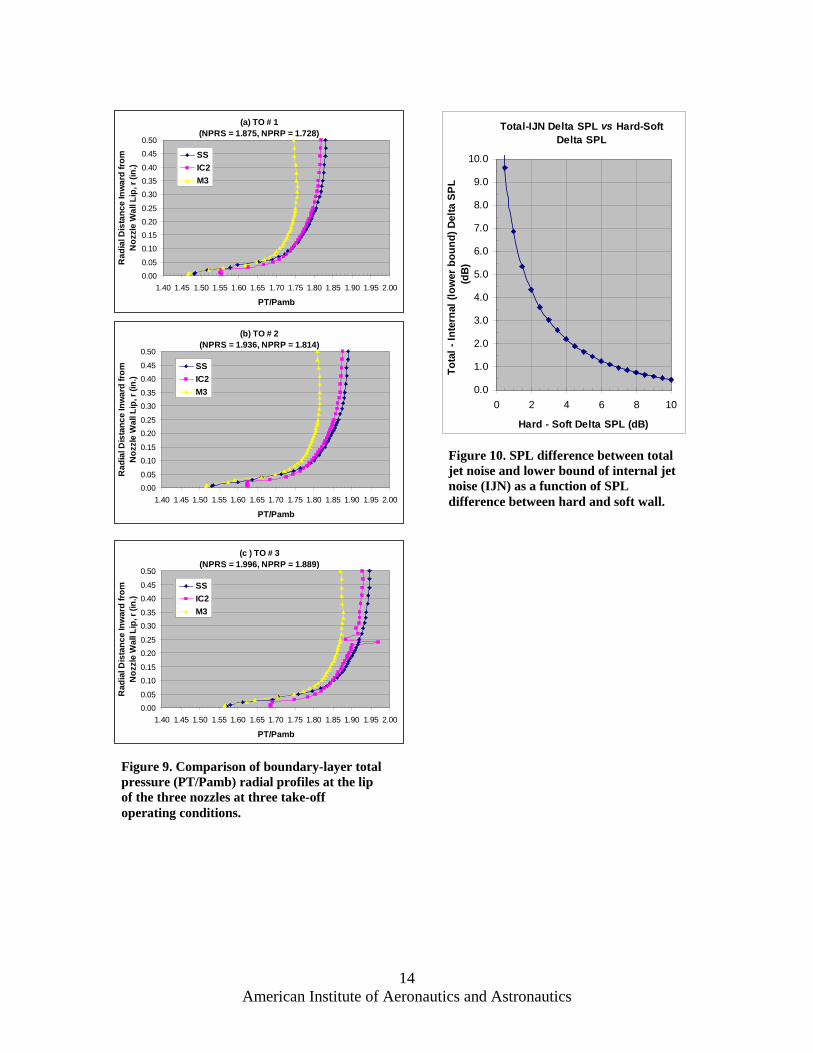
Lastly, Fig. 9 captures the internal boundary layer profiles at the exit plane of these three nozzles in terms of the non-dimensionalized total pressure, PT/Pamb, at three different conditions. For all three conditions, the lobe mixer has lower total pressure than the internal chevrons, which in turn has slightly lower values than the simple splitter. The maximum values, which appear to have roughly reached their asymptotic values within the half-inch radial scan, are less than the total pressures of fan stream at the charging stations far upstream, and represent losses due to mixing amongst other losses. In particular the asymptotic values for the lobe mixer are less than those for internal chevron or simple splitter nozzles. Hence, if we consider the boundary layer “thickness” as corresponding to a certain percentage (say, 95%) of the asymptotic value of the total pressure near the wall, then such a boundary layer thickness is less for lobe mixers than it is for internal chevrons. Such boundary layer profile data can be useful when designing the “immersion’ values for external chevrons and can also be used for validation of CFD prediction codes for internally mixed nozzles.

B. Internal Noise From the discussion in the previous section there is reasonable evidence that internal chevrons IC2 are gentler

mixers than lobe mixer M3, and we would like to investigate what that internal mixing noise contributes to the far field noise. As mentioned earlier, the author has previously studied this situation for lobe mixer (M3) and simple splitter (SS) using the technique of hardwall/softwall difference, and the same technique will be applied for the case of internal chevrons IC2. Previously, only the sound pressure level (SPL) difference between the hard-wall nozzle and the soft-wall nozzle were obtained and it was mentioned that it gives an indication of the lower bound on the contribution of internal noise to far field, without actually finding this lower bound. Here, we will find this lower bound as obtained by the hardwall/softwall technique for not only the internal chevrons IC2 but also for the previous cases of lobe mixer M3 and simple splitter SS.

If we assume that (a) the total sound field at far field points is a sum of noise radiated from an effective external noise source and an effective internal noise source, (b) the effective internal and external noise sources are uncorrelated, (c) the softwall does not change the external flow, and (d) the softwall completely absorbs the internal sound, then we can show that the internal sound pressure level (SPL) can be written as:

10int 10 log 1 10ernal hardwall

hardwall softwall

SPL SPL

SPL SPL

∆−⎛ ⎞

= + −⎜ ⎟⎝ ⎠

∆ = −


6

Although the first three assumptions are very reasonable, the last one is not necessarily a good assumption. In practice, the softwall can never completely absorb the internally generated sound because (a) some acoustic rays (representative of high frequency sound) can escape from internal sources to far field regions without ever interacting with the nozzle wall, and (b) the soft wall does cannot absorb all the sound that is incident upon it at all frequencies. This acoustic leakage of internal sound in the softwall case is a function of directivity angle and frequency and can be easily shown to always give a positive contribution to the right hand side of the above equation. Hence, the above equation for the internal sound actually becomes a lower bound for the internal sound contribution to far field.

In order to appreciate how ∆ is related to the difference between the total noise (or hard wall noise) and the

lower bound of this internal noise, we plot ⎟⎟⎠

⎞⎜⎜⎝

⎛−−

∆−

10101log10 as a function of ∆ in Fig. 10. As the difference

between the hardwall and the softwall noise, ∆, increases it shows that the internal noise contributes more and more to the total noise. For example, when the difference between the hard wall and the soft wall noise is 3 dB, this plot shows that the internal jet noise contribution to far field noise is at most within 3 dB of the total noise – in other words, the internal noise contributes at least as much to the far field noise as external noise. For lower values of ∆ the lower bound of internal noise contribution to far field noise becomes smaller and smaller.

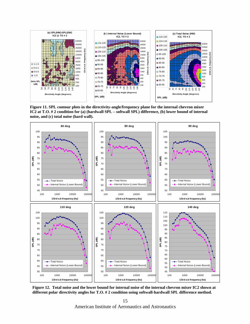
Figure 11(a) shows ∆, the SPL difference between the hardwall and the softwall nozzles, for the internal chevron nozzle, IC2, with 18 chevrons at TO # 2 condition at static wind-tunnel conditions. These are contour plots in the frequency-directivity plane of the difference between the SPL with hardwall and softwall nozzle for a given mixer obtained from the polar array of microphones placed in the far field at 25 ft. The SPL values have been normalized to standard acoustic day conditions to remove differences in the test-day conditions during the hardwall and softwall nozzle tests. Repeatability in these acoustic tests at LSAF is ±0.5 dB, so that anything above 0.5 dB is considered actual physical difference. The strongest contribution appears at 90 deg. and very high frequencies, although the low values of ∆ = 1 to 1.5 there suggest that the contribution of internal jet noise (IJN) from internal chevrons to far field total noise even there is at most 5 to 5.5 dB less than the total noise.

Fig. 12 shows this lower bound for IC2 on IJN spectra as compared to the total noise at different angles. The lower bound simply implies that at any angle, say, 90 deg. at any given frequency, IJN is at least as much as shown in this figure – but it can be higher, the uncertainty arising from the leakage contribution mentioned earlier. For low frequencies, the contribution is far lower, but the IJN contribution at higher frequencies at 90 deg. gets closer to the total noise. At very shallow angles, like 140 deg., the contribution at peak SPL frequencies is higher than at higher frequencies.

Figure 11(b) shows the lower bound on IJN as a contour plot in the directivity-frequency plane to get an appreciation of the relative SPL magnitudes at different angles and frequencies. It can be compared to that for the total noise shown in Fig. 11(c). Interestingly, the general characteristics of IJN appear to be similar to that of the total noise with peak values at shallow angles (like 140 deg.) and low frequencies (800 hz). The total noise has this characteristics because the external jet mixing noise, which is seen to dominate the far field, arises from the end of the potential core and is well-known to have this source directivity. On the other hand, for internal jet noise it is possible to explain this by noting that all the sound that radiates in the duct in the axial direction simply must refract to the critical angle bordering the so-called “zone of silence” for a parallel jet which is close to these shallow angle values.

Thus, the hardwall/softwall SPL difference contour plots capture where in the directivity-frequency plane the softwall can influence most, thus depicting the dominance of the relative contribution of internal jet noise to total noise for a given mixer nozzle; whereas, IJN contour plots show where in this directivity-frequency plane IJN itself dominates. Both are useful but different pieces of information which help understand these IJN characteristics.

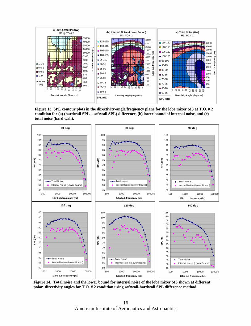
Figure 13 shows these same contour plots for the lobe mixer M3. Fig. 13(a) shows that the lobe mixer has similar contribution from IJN to the total noise but is at wider angles around 90 deg. This can also be seen in the IJN spectral plots of Fig. 14. However, Fig. 13(c) shows that the total noise of M3 is far less than that of this internal chevron mixer IC2 under static wind-tunnel conditions. Interestingly, Fig. 13(b) shows that the peak value of the lower bound for IJN for M3 (at 140 deg.) is lower than that for the internal chevron mixer.

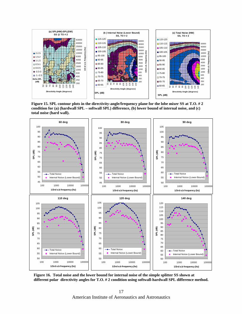
Figures 15 and 16 show these similar plots for the simple splitter nozzle, SS, at the same conditions. It is very interesting to see that Fig. 15(a) shows that IJN contributes fairly strongly (difference is 1.5-2.5 dB) at higher frequencies near 90 deg., as opposed to the lower contribution to IJN to total noise of internal chevrons, IC2, (see Fig. 11(a)), but the IJN and total noise spectral/directivity characteristics are very similar to that of the internal chevrons.


7

Since all these are only lower bounds on IJN and not IJN values themselves it may not be apt to compare IJN of one mixer nozzle against the other. However, these lower bounds can be used to check the validity of predictive methods. For example, any internal jet noise prediction method for such internally-mixed nozzles should give results which are at least above these lower bounds for IJN – that by itself is very useful, since at present there is nothing in the literature which extracts these internal jet noise contributions to validate prediction methods. The results for the simple splitter nozzle with simplistic two-plug flows may be a useful start and the author has started developing along those lines for internal jet noise propagation inside a very long duct.9

Another useful fact that seems to emerge from all these IJN plots is the emergence of a spectral hump of IJN at higher frequencies. If we assume that very low SPL differences between hardwall and softwall nozzles can be discarded as giving the correct spectral characteristics of IJN (and this occurs at low frequencies), then there appears to exist a hump in the IJN spectra located at fairly high frequencies (10-20 KHz). This is most clearly seen for M3 at 90 deg. This may not be true at all angles, however. Such a secondary hump from IJN located at relatively high frequencies, if it really exists, can complement the other two well-known spectral humps arising from external jet mixing noise, namely, the dominant low frequency hump from large-scale eddies near the end of the potential core, and the “mid-frequency” hump from fine scale turbulence near the nozzle exit plane.

IV. Summary An experimental study was conducted to understand the internal flow and noise characteristics of internal

chevrons and lobe mixers. This was achieved by developing two extra pieces of hardware for the external nozzle: a uniquely instrumented nozzle with internal total temperature rakes which can rotate with respect to the internal mixer to give the flow properties in the azimuthal direction at several axial stations, and a softwall nozzle to deduce the lower bound on internal jet noise contribution to the far field noise. The boundary layer profiles obtained at the nozzle exit plane can be useful in selecting the appropriate immersions for external chevrons on such nozzles.

The internal chevron mixer appears to have lower mixing between the primary and the secondary stream, as expected, and also lower internal noise contribution to the far field noise. The lobe mixer has much stronger mixing, as expected, and has slightly higher internal jet noise contribution to far field. A simple splitter nozzle was also tested and, interestingly, shows strong contribution from internal jet noise to far field although the absolute internal jet noise spectral-directivity characteristics are very similar to that of the internal chevron mixer. This may be the result of high shear between the two streams in the simple splitter nozzle and should be amenable to theoretical investigation.

Besides the better understanding obtained from this study, the database generated for several internally mixed nozzles can be used to validate both CFD flow predictions inside the nozzle and any predictive theory for internal jet noise.

References 1Mengle, V. G., “Jet Noise Characteristics of Chevrons in Internally Mixed Nozzles,” AIAA Paper 2005-2934. 2Mengle, V. G., “Internal Jet Noise Diagnostics for Internally Mixed Nozzles,” AIAA Paper 2004-2900. 3Mengle, V. G. and Dalton, W. N., “Lobed Mixer Design for Noise Suppression. Acoustic and Aerodynamic Test Data Analysis,” NASA CR-2002-210823, Vol. 1, July 2002. 4Mengle, V. G., “Relative Clocking of Enhanced Mixing Devices for Jet Noise Benefit,” AIAA Paper 2005-0996. 5Greitzer, E.M., Tan, C.S. and Graf, M.B., Internal Flow – Concepts and Applications, Cambridge Univ. Press, Cambridge, U.K., 2004, Section 9.9. 6Waitz, I., Qiu, Y.J., Manning, T.A., Fung A.K.S., Elliot, J.K., Kerwin, J.M., Krasodebski, J.K., O’Sullivan, M.N., Tew, D.E., Greitzer, E.M., Marble, F.E., Tan, C.S. and Tillman, “Enhanced Mixing with Streamwise Vorticity,” Prog. Aerospace Sci., 33, No. 5-6, 1997, pp. 323-351. 7Patterson, R.W., “Turbofan Forced Mixer-Nozzle Internal Flow Field I – A Benchmark Experimental Study,” NASA CR 3492, April 1982. 8Yu, S.C.M. and Xu, X.G., “Turbulent Mixing of Coaxial Nozzle Flows with a Central-Lobed Mixer,” J. Prop. & Power, Vol. 13, No. 4, July-August 1997, pp. 517-524. 9Mengle, V.G., “Jet Noise Propagation in Ducts of Arbitrary Cross-Section with Parallel Sheared Flows,” AIAA Paper 2003-3284.


8

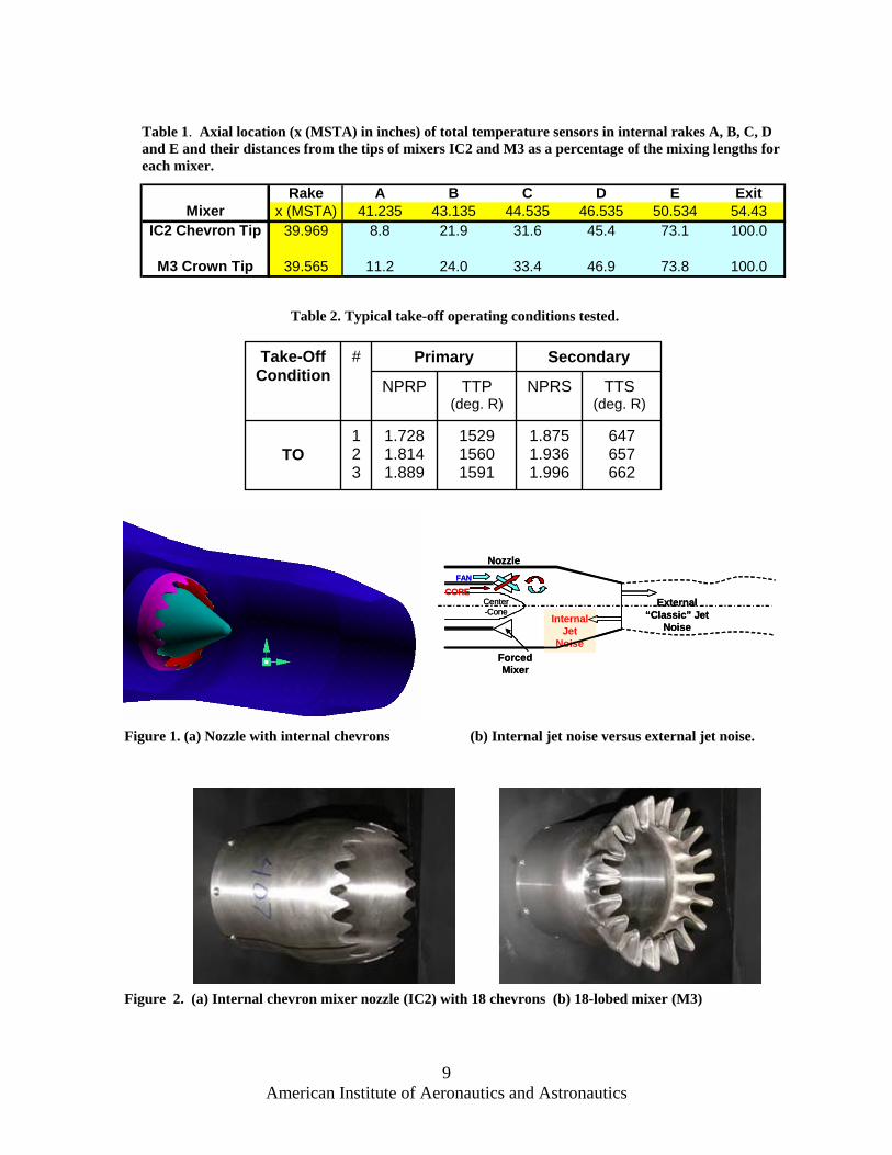
Rake A B C D E ExitMixer x (MSTA) 41.235 43.135 44.535 46.535 50.534 54.43

IC2 Chevron Tip 39.969 8.8 21.9 31.6 45.4 73.1 100.0

M3 Crown Tip 39.565 11.2 24.0 33.4 46.9 73.8 100.0

Table 1. Axial location (x (MSTA) in inches) of total temperature sensors in internal rakes A, B, C, D and E and their distances from the tips of mixers IC2 and M3 as a percentage of the mixing lengths for each mixer.

647 657 662

1.8751.936 1.996

15291560 1591

1.7281.814 1.889

12 3

TO

TTS (deg. R)

NPRSTTP(deg. R)

NPRP

Secondary Primary#Take-Off Condition

Table 2. Typical take-off operating conditions tested.

Internal Jet

Noise

External “Classic” Jet

Noise

Nozzle

Forced Mixer

FAN

Center-Cone

CORE

Internal Jet

Noise

External “Classic” Jet

Noise

Nozzle

Forced Mixer

FAN

CORECenter-Cone

Figure 1. (a) Nozzle with internal chevrons (b) Internal jet noise versus external jet noise.

Figure 2. (a) Internal chevron mixer nozzle (IC2) with 18 chevrons (b) 18-lobed mixer (M3)


9

LSAF

Wake RakeNozzle with Removable &

Rotatable TT Rakes Figure 3. Instrumentation used to explore the

internal flow field and also the external flow field for internally mixed nozzles.

Boundary

Layer Probe

A B C D E T x1 x2 x3

a b c d e

C/L

A B C D E T x1 x2 x3

a b c d e

C/L

A (0º)

D (270º)

B, T (180º)

E (135º)

PA (50º)

C (90º)

PB (220º)

A (0º)

D (270º)

B, T (180º)

E (135º)

PA (50º)

C (90º)

PB (220º)

Figure 4. (a) Relative axial locations (not to scale) of internal rake TT sensors (A-E), lip boundary-layer probe (T), external wake rake (x1- x3) and some salient features of the nozzle: a = mixer tip, b = start of outer straight cylindrical section nozzle (x(MSTA) = 41.405”), c = plug tip (x(MSTA) = 43.750”), d = end of straight cylindrical section nozzle (x(MSTA) = 48.291”) and e = exit plane of nozzle (x(MSTA) = 54.43”). (b) Relative azimuthal locations (clockwise from rake A, looking forward) of the internal rakes (A-E), boundary layer probe (T) and static-pressure wall taps (PA, PB).


10

Array A @ 0 deg

1.2

1.25

1.3

1.35

1.4

1.45

1.5

1.55

1.6

1.65

40 42 44 46 48 50 52 54X, Axial Distance (in.)

PS/P

AM

B

SSIC2M3

Figure 5. Wall static pressure comparison for the three nozzles SS (simple splitter), IC2 (internal chevrons) and lobe mixer (M3) at TO # 2 condition with NPRS = 1.936.

Ra

ke A

600

700

800

900

1000

1100

1200

1300

1400

1500

1600

1.5 2 2.5 3 3.5 4

radius (in.)

TT (d

eg R

)

0 deg w/ 2 rakes

0 deg w/ 4 rakes

4 deg w/ 2 rakes

4 deg w/ 4 rakes

8 deg w/ 2 rakes

8 deg w/ 4 rakes

12 deg w/ 2 rakes

12 deg w/ 4 rakes

16 deg w/ 2 rakes

16 deg w/ 4 rakes

Rake D

600

650

700

750

800

850

900

950

1000

1050

1100

0.5 1 1.5 2 2.5 3 3.5 4

radius (in.)

TT (d

eg R

)

0 deg w/ 2 rakes0 deg w/ 4 rakes4 deg w/ 2 rakes4 deg w/ 4 rakes8 deg w/ 2 rakes8 deg w/ 4 rakes12 deg w/ 2 rakes12 deg w/ 4 rakes16 deg w/ 2 rakes16 deg w/ 4 rakes

Figure 6. Rake-to-rake interference effect due to the use of two rakes (A and B, or C and D) and all four rakes (A, B, C and D) shown for rakes A and D for several azimuthal angles (0, 4, 8, 12 and 16 degrees) using 18-lobed mixer (M3) at TO # 2 condition.


11

0 2 4 6 8 10 12 14 16 18 201.91

2.21

2.51

2.81

3.11

3.41

3.71

TT

Theta (deg)

radi

us (i

n)

Rake A1500-15751425-15001350-14251275-13501200-12751125-12001050-1125975-1050900-975825-900750-825675-750600-675

0 2 4 6 8 10 12 14 16 18 201.11

1.71

2.11

2.51

2.81

3.11

3.41

3.71

TT

Theta (deg)

radi

us (i

n)

Rake B

1350-14251275-13501200-12751125-12001050-1125975-1050900-975825-900750-825675-750600-675

0 2 4 6 8 10 12 14 16 18 200.51

1.11

1.71

2.11

2.51

2.81

3.11

3.41

3.71

TT

Theta (deg)

radi

us (i

n)

Rake C

1500-15751425-15001350-14251275-13501200-12751125-12001050-1125975-1050900-975825-900750-825675-750600-675

0 2 4 6 8 10 12 14 16 18 200.51

1.11

1.71

2.11

2.51

2.81

3.11

3.41

3.71

TT

Theta (deg)

radi

us (i

n)

Rake D 1500-1575

1425-1500

1350-1425

1275-1350

1200-1275

1125-1200

1050-1125

975-1050

900-975

825-900

750-825

675-750

600-675

0 2 4 6 8 10 12 14 16 18 201.11

1.71

2.11

2.51

2.81

3.11

3.41

3.71

TT

Theta (deg)

radi

us (i

n)

Rake B

1350-14251275-13501200-12751125-12001050-1125975-1050900-975825-900750-825675-750600-675

0 2 4 6 8 10 12 14 16 18 200.51

1.11

1.71

2.11

2.51

2.81

3.11

3.41

3.71

TT

Theta (deg)

radi

us (i

n)

Rake C

1350-14251275-13501200-12751125-12001050-1125975-1050900-975825-900750-825675-750600-675

0 2 4 6 8 10 12 14 16 18 200.51

1.11

1.71

2.11

2.51

2.81

3.11

3.41

3.71

TT

Theta (deg)

radi

us (i

n)

Rake D1350-1425

1275-1350

1200-1275

1125-1200

1050-1125

975-1050

900-975

825-900

750-825

675-750

600-675

0 2 4 6 8 10 12 14 16 18 201.91

2.21

2.51

2.81

3.11

3.41

3.71

TT

Theta (deg)

radi

us (i

n)

Rake A

1500-15751425-15001350-14251275-13501200-12751125-12001050-1125975-1050900-975825-900750-825675-750600-675

Figure 7. Axial evolution of total temperature over one azimuthal period inside the nozzle using internal rakes A-E (two at a time) at TO # 2 condition for (a) nozzle with 18 internal chevrons, IC2, (left column), and (b) 18-lobed mixer M3 (right column), (continued on next page for Rake E).


12

0 2 4 6 8 10 12 14 16 18 200.504

1.004

1.504

1.904

2.304

2.604

2.904

3.204

3.504

TT

Theta (deg)

radi

us (i

n)

Rake E 1500-1575

1425-1500

1350-1425

1275-1350

1200-1275

1125-1200

1050-1125

975-1050

900-975

825-900

750-825

675-750

600-675 0 2 4 6 8 10 12 14 16 18 200.504

1.004

1.504

1.904

2.304

2.604

2.904

3.204

3.504

TT

Theta (deg)

radi

us (i

n)

Rake E 1350-1425

1275-1350

1200-1275

1125-1200

1050-1125

975-1050

900-975

825-900

750-825

675-750

600-675

Figure 7. (continued) (for caption see previous page)

7 6 5 4 3 2 1 0 -1 -2 -3 -4 -5 -6

500575650725800875950

102511001175125013251400147515501625

TT (deg. R)

Z-axis (in.)

Y-axis (in.)

SS, X = 3.125 in. 1550-1625

1475-1550

1400-1475

1325-1400

1250-1325

1175-1250

1100-1175

1025-1100

950-1025

875-950

800-875

725-800

650-725

575-650

500-575

75.

75 4.5

3.25 2

0.75

-0.5

-1.7

5 -3

-4.2

5

-5.5

500575650725800875950

102511001175125013251400147515501625

TT (deg. R)

Z-axis (in.) Y-axis (in.)

IC2, X = 3.125 in. 1550-1625

1475-1550

1400-1475

1325-1400

1250-1325

1175-1250

1100-1175

1025-1100

950-1025

875-950

800-875

725-800

650-725

575-650

500-575

7

5.87

5

4.75

3.62

5

2.5

1.37

5

0.25

-0.8

75 -2

-3.1

25

-4.2

5

-5.3

75

-1.75

1.125500550600650700750800850900950

10001050

00

TT (deg. R)

Z-axis (in.)

Y-axis (in.)

M3, X = 3.125 in. 1050-1100

1011 00-1050

950-1000

900-950

850-900

800-850

750-800

700-750

650-700

600-650

550-600

500-550

Figure 8. Comparison of total temperature profiles for various nozzles outside the nozzle at X/D = 0.469. Simple splitter (SS) is also shown.


13

(a) TO # 1(NPRS = 1.875, NPRP = 1.728)

0.00

0.05

0.10

0.15

0.20

0.25

0.30

0.35

0.40

0.45

0.50

1.40 1.45 1.50 1.55 1.60 1.65 1.70 1.75 1.80 1.85 1.90 1.95 2.00

PT/Pamb

Rad

ial D

ista

nce

Inw

ard

from

N

ozzl

e W

all L

ip, r

(in.

)

SSIC2M3

(b) TO # 2(NPRS = 1.936, NPRP = 1.814)

0.000.05

0.10

0.15

0.20

0.25

0.300.35

0.40

0.45

0.50

1.40 1.45 1.50 1.55 1.60 1.65 1.70 1.75 1.80 1.85 1.90 1.95 2.00

Rad

ial D

ista

nce

Inw

ard

from

N

ozzl

e W

all L

ip, r

(in.

)

PT/Pamb

SSIC2M3

(c ) TO # 3(NPRS = 1.996, NPRP = 1.889)

0.00

0.05

0.10

0.15

0.20

0.25

0.300.35

0.40

0.45

0.50

1.40 1.45 1.50 1.55 1.60 1.65 1.70 1.75 1.80 1.85 1.90 1.95 2.00

PT/Pamb

Rad

ial D

ista

nce

Inw

ard

from

N

ozzl

e W

all L

ip, r

(in.

)

SSIC2M3

Figure 9. Comparison of boundary-layer tpressure (PT/Pamb) radial profiles at the lipof the three nozzles at three take-off operating conditions.

otal

Total-IJN Delta SPL vs Hard-Soft Delta SPL

0.0

1.0

2.0

3.0

4.0

5.0

6.0

7.0

8.0

9.0

10.0

0 2 4 6 8 10

Hard - Soft Delta SPL (dB)

Tota

l - In

tern

al (l

ower

bou

nd) D

elta

SP

L (d

B)Figure 10. SPL difference between total jet noise and lower bound of internal jet noise (IJN) as a function of SPL difference between hard and soft wall.


14


15

50 60 70 80 90 100

110

120

130

140

160250

400630100016002500400063001000016000250004000063000

De

lta SPL (dB)

Directivity Angle (degrees)

1/3

rd o

.b. F

requ

ency

(hz)

(a) SPL(HW)-SPL(SW)IC2 @ TO # 2

1-1.50.5-10-0.5-1-0

50 60 70 80 90 100

110

120

130

140

160250

400630100016002500

40006300100001600025000

4000063000

SPL (dB)Directivity Angle (degrees)

1/3r

d o.

b. fr

eque

ncy

(hz)

(c) Total Noise (HW)IC2, TO # 2115-120

110-115

105-110

100-105

95-100

90-95

85-90

80-85

75-80

70-75

65-70

60-65

50 60 70 80 90 100

110

120

130

140

160

250

400630

1000

1600

2500

4000

630010000

16000

25000

40000

63000

SPL (dB)


1/3r

d o.

b. fr

eque

ncy

(hz)

(b ) Internal Noise (Lower Bound)IC2, TO # 2

115-120

110-115

105-110

100-105

95-100

90-95

85-90

80-85

75-80

70-75

65-70

60-65

Figure 11. SPL contour plots in the directivity-angle/frequency plane for the internal chevron mixer IC2 at T.O. # 2 condition for (a) (hardwall SPL – softwall SPL) difference, (b) lower bound of internal noise, and (c) total noise (hard wall).

60 deg

45

50

55

60

65

70

75

80

85

90

95

100

100 1000 10000 100000

1/3rd o.b frequency (hz)

SPL

(dB

)

Total NoiseInternal Noise (Lower Bound)

80 deg

45

50

55

60

65

70

75

80

85

90

95

100

100 1000 10000 100000


SPL

(dB

)


90 deg

50

55

60

65

70

75

80

85

90

95

100

105

100 1000 10000 100000


SPL

(dB

)


110 deg

50

55

60

65

70

75

80

85

90

95

100

105

100 1000 10000 100000


)L

(dB

SP


120 deg

50

55

60

65

70

75

80

85

90

95

100

105

100 1000 10000 100000


SPL

(dB

)


140 deg

45

50

55

60

65

70

75

80

85

90

95

100

105

110

115

100 1000 10000 100000


SPL

(dB

)


Figure 12. Total noise and the lower bound for internal noise of the internal chevron mixer IC2 shown at different polar directivity angles for T.O. # 2 condition using softwall-hardwall SPL difference method.


16

50 60 70 80 90 100

110

120

130

140

160250

400630100016002500400063001000016000250004000063000

Delta SPL (dB)

Directivity Angle (degrees)1/

3 rd

o.b

. Fre

quen

cy (h

z)

(a) SPL(HW)-SPL(SW)M3 @ TO # 2

1-1.50.5-10-0.5-1-0

50 60 70 80 90 100

110

120

130

140

160250400630100016002500

400063001000016000250004000063000


1/3r

d o.

b. fr

eque

ncy

(hz)

(b ) Internal Noise (Lower Bound)M3, TO # 2

115-120

110-115

105-110

100-105

95-100

90-95

85-90

80-85

75-80

70-75

65-70

60-65 50 60 70 80 90 100

110

120

130

140

160250400630100016002500

400063001000016000250004000063000


1/3r

d o.

b. fr

eque

ncy

(hz)

(c) Total Noise (HW)M3, TO # 2

115-120

110-115

105-110

100-105

95-100

90-95

85-90

80-85

75-80

70-75

65-70

60-65

Figure 13. SPL contour plots in the directivity-angle/frequency plane for the lobe mixer M3 at T.O. # 2 condition for (a) (hardwall SPL – softwall SPL) difference, (b) lower bound of internal noise, and (c) total noise (hard wall).

60 deg

45

50

55

60

65

70

75

80

85

90

95

100

100 1000 10000 100000


SPL

(dB

)


80 deg

45

50

55

60

65

70

75

80

85

90

95

100

100 1000 10000 100000


SPL

(dB

)


90 deg

50

55

60

65

70

75

80

85

90

95

100

105

100 1000 10000 100000


SPL

(dB

)


Figure 14. Total noise and the lower bound for internal noise of the lobe mixer M3 shown at different polar directivity angles for T.O. # 2 condition using softwall-hardwall SPL difference method.

110 deg

50

55

60

65

70

75

80

85

90

95

100

105

100 1000 10000 100000


SPL

(dB

)


120 deg

50

55

60

65

70

75

80

85

90

95

100

105

100 1000 10000 100000


SPL

(dB

)


140 deg

45

50

55

60

65

70

75

80

85

90

95

100

105

110

115

100 1000 10000 100000


SPL

(dB

)


50 60 70 80 90 100

110

120

130

140

160250

400630100016002500400063001000016000250004000063000

Delta SPL (dB)


1/3

rd o

.b. F

requ

ency

(hz)

(a) SPL(HW)-SPL(SW)SS @ TO # 2

2-2.51.5-21-1.50.5-10-0.5-0.5-0-1--0.5

50 60 70 80 90 100

110

120

130

140

160250400630100016002500

400063001000016000250004000063000

SPL (dB)


1/3r

d o.

b. fr

eque

ncy

(hz)

(b ) Internal Noise (Lower Bound)SS, TO # 2

115-120

110-115

105-110

100-105

95-100

90-95

85-90

80-85

75-80

70-75

65-70

60-65

50 60 70 80 90 100

110

120

130

140

160250400630100016002500400063001000016000250004000063000


1/3r

d o.

b. fr

eque

ncy

(hz)

(c) Total Noise (HW)SS, TO # 2

115-120

110-115

105-110

100-105

95-100

90-95

85-90

80-85

75-80

70-75

65-70

60-65

Figure 15. SPL contour plots in the directivity-angle/frequency plane for the lobe mixer SS at T.O. # 2 condition for (a) (hardwall SPL – softwall SPL) difference, (b) lower bound of internal noise, and (c) total noise (hard wall).

60 deg

45

50

55

60

65

70

75

80

85

90

95

100

100 1000 10000 100000


SPL

(dB

)


80 deg

45

50

55

60

65

70

75

80

85

90

95

100

100 1000 10000 100000


SPL

(dB

)


90 deg

50

55

60

65

70

75

80

85

90

95

100

105

100 1000 10000 100000


SPL

(dB

)


110 deg

50

55

60

65

70

75

80

85

90

95

100

105

100 1000 10000 100000


SPL

(dB

)


120 deg

50

55

60

65

70

75

80

85

90

95

100

105

100 1000 10000 100000


SPL

(dB

)


140 deg

50

55

60

65

70

75

80

85

90

95

100

105

110

115

120

100 1000 10000 100000


SPL

(dB

)


Figure 16. Total noise and the lower bound for internal noise of the simple splitter SS shown at different polar directivity angles for T.O. # 2 condition using softwall-hardwall SPL difference method.


17

Documents

AIAA-2006-0623-Internal Flow Noise