1

Age and socioeconomic inequalities in health: examining the role

of lifestyle choices

Abstract

The role of lifestyle choices in explaining how socioeconomic inequalities in health vary with

age has received little attention. This study explores how the income and education gradients

in both important lifestyle choices and self-assessed health (SAH) vary with age. Repeated

cross-sectional data from Norway (n =25,016) and logistic regression models are used to track

the income and education gradients in physical activity, smoking, consumption of fruit and

vegetables and SAH over the age range 25–79 years. The education gradient in smoking, the

income gradient in consumption of fruit and vegetables and the education gradient in physical

activity among males become smaller at older ages. Physical activity among females is the

only lifestyle indicator in which the income and education gradients grow stronger at older

ages. In conclusion, this study shows that income and education gradients in lifestyle choices

may not remain constant, but vary with age, and such variation could be important in

explaining corresponding age patterns of inequality in health.

Keywords: Socioeconomic status; Inequality; Life course; Lifestyles; Health; Norway

1. Introduction

A large and growing body of literature seeks to improve our understanding of why indicators

of socioeconomic status and health are so strongly associated (Marmot et al., 2008; Cutler et

al., 2011). Acknowledging the dynamic nature of health production, this literature has partly

focused on how socioeconomic inequalities in health evolve over the adult life course. The

current empirical evidence on this important issue is mixed, in part because different

2

indicators of socioeconomic status and health have been investigated (Kim & Durden, 2007).

However, three main patterns of results stand out.

In some studies, health differences by socioeconomic status are found to be increasing

in age throughout the adult life course (Benzeval et al., 2011; Kim & Durden, 2007; Ross &

Wu, 1996; Wilson et al., 2007). Such results correspond with the cumulative advantage

hypothesis. This hypothesis asserts that throughout the adult life course, socioeconomic status

is closely associated with our daily investments into the production of poor and good health.

Gradually, these investments result in a relatively more rapid deterioration of health among

lower than higher socioeconomic status groups.

In other studies, health differences by socioeconomic status are found to be increasing

in age until late midlife, or pre-retirement (50–60 years of age), after which they level off or

begin to decrease (Beckett, 2000; Huijts et al., 2010; van Kippersluis et al., 2010). Such

results are in line with the cumulative advantage hypothesis until late midlife, but with an age-

as-leveler hypothesis thereafter. More particularly, biological factors become increasingly

important with older age in determining health, thus downplaying the role of socioeconomic

status (Herd, 2006). Also other factors have been found to contribute to age-as-leveler effects

in health. These factors include the effects of mortality selection (Kim & Durden, 2007),

cohort effects (Lynch, 2003) and labor market participation status (van Kippersluis et al.,

2010; Case & Deaton, 2005).

Finally, some studies have found that, for selected health and socioeconomic status

indicators, health differences by socioeconomic status do not vary significantly with age (Kim

& Durden, 2007; Beckett, 2000). We refer to such patterns of results as being in line with the

persistent health inequality hypothesis (Ferraro & Farmer, 1996).

To the best of our knowledge, no studies have yet explicitly examined the potential

role of healthy lifestyle choices in explaining these competing hypotheses for the dynamics of

3

socioeconomic inequalities in health. This is surprising for at least three reasons. First, there is

convincing evidence for the protective effect of certain lifestyle choices, including physical

activity, not smoking and consumption of fruit and vegetables, against adverse health

outcomes such as type 2 diabetes, cardiovascular disease and certain types of cancer (World

Health Organization, 2003; He et al., 2007; Jeon et al., 2007; Gandini et al., 2008; Sofi et al.,

2008). Second, similar to most health outcomes, the probability of making healthy lifestyle

choices is closely associated with socioeconomic status indicators such as education and

income (Pampel et al., 2010; Cutler & Lleras-Muney, 2010). Third, the effects of healthy

lifestyle choices on the incidence of adverse health outcomes are often characterized by

cumulative, long-processes (Kuh & Shlomo, 2004), which highlights the importance of taking

a life course perspective with respect to the dynamic relationship between socioeconomic

status, lifestyle choices and health.

As noted, we often implicitly assume that lifestyle choices differ systematically by

socioeconomic status and thereby contribute to patterns of cumulative advantage effects in

health. This is a reasonable assumption to the extent that the socioeconomic gradients in

lifestyle choices remain stable or increase over the adult life course. But what if the

socioeconomic gradients in lifestyle choices become smaller with older age? For example,

people of lower socioeconomic status may grow more health conscious and thus engage in

healthier lifestyles when they reach late midlife and realize that good health investments are

important for longevity.

We use repeated cross-sectional data from Norway from 1997–2011 to explore how

the income and education gradients in both important lifestyle choices and SAH vary with

age. Repeated cross-sectional data are often referred to as pseudo-panel data because although

not tracking the same individuals as they age, such data allow for tracking the average age

patterns for groups of individuals as they age while controlling for possibly confounding

4

cohort and period effects (Deaton, 1997). However, note that our study is not a pure ‘life

course’ study in the sense that we do not follow the same individuals as they age.

Our lifestyle indicators are physical activity, smoking and consumption of fruit and

vegetables. We use these lifestyle indicators because they are different in nature and because

of their close association with both socioeconomic status indicators and the risk of major

health outcomes, as described above. Our research questions are as follows. First, to what

extent are the observed age patterns of inequality in lifestyle choices consistent with (i) the

age-as-leveler, (ii) the persistent health inequality, and (iii) the cumulative advantage

hypothesis in health? Second, to what extent do age patterns of inequality vary across

different lifestyle choices, education and income, and gender?

2. Methods

2.1. Data source

The Norwegian Monitor Survey is a nationally representative and repeated cross-sectional

survey of adults aged 15–95 years. The survey has been conducted every second year since

1985 and is one of Norway’s most comprehensive consumer and opinion surveys. The

institution behind the survey (Ipsos Norway) recruits respondents through a short telephone

interview, and those who accept to participate receive a paper-based questionnaire by mail.

Ethical approval was not required for this research; we represent a third party user of the data

in question, and we only have access to a data file that contains anonymous data, i.e., we do

not have access to any information that can be used to identify specific individuals.

The question about SAH was not included in the survey before 1997, and therefore

data from 1997 to 2011 are used. For two reasons, only respondents between the ages of 25

and 79 years were included. First, we want to study individuals who have completed most of

their education and started earning their own income. Second, the sample includes relatively

5

few respondents between the ages of 80 and 95 years. After deleting observations with

missing information for any of the variables included in this study (3,066 observations), we

obtain our sample of 25,016 observations. Based on statistical tests comparing group means,

the deleted respondents were on average significantly older, more likely female, less educated

and had lower incomes than the respondents that are included in the sample.

2.2. Outcome variables

The survey questions related to physical activity, smoking, consumption of fruit and

vegetables and SAH are based on various types of categorical scales. The respondents were

asked to indicate their frequency of intake for nine different fruit and vegetables on the

following scale; “daily”; “3−5 times per week”; “1−2 times per week”; “2−3 times per

month”; “about once per month”; “3−11 times per year”; “rarer”; or “never”. Similarly,

physical activity has an 8-point frequency scale ranging from “never” to “once or more per

day”. The respondents also indicated if they smoked tobacco “daily”, “sometimes” or “never”

at the time of the survey, whereas SAH is based on the typical 5-point scale ranging from

“very poor” to “very good” health. To facilitate the comparison of how income and education

gradients vary with age, we have dichotomized each of these categorical variables. We define

being physically active at least twice per week, not a daily smoker (non-smoking), eating fruit

and vegetables at least twice per day and reporting one’s SAH to be “good” or “very good” as

binary indicators of healthy lifestyles and good health.

2.3. Explanatory variables

We categorize education into four groups using dummy indicators, ranging from having

completed only lower secondary education (9 years of education) or less, to having obtained a

university or college degree. We divide household income into age-group survey-year specific

6

income quartiles, with each age group comprising a 5-year interval (e.g., people aged 25–29

years). The original survey question on household income included nine response alternatives,

each representing a specific income interval. Before dividing income into age-group survey-

year specific quartiles, we (i) set household income to the midpoint value of each income

interval, and (ii) adjusted for household size by dividing the resulting income measure by the

square root of household size (OECD, 2008).

We define age as a continuous variable, but center it at age 30 to reduce

multicollinearity between age and age-squared in the later statistical analyses (Kim & Durden,

2007). Dichotomous indicators for gender, survey years and 5-year birth cohorts are also

included in the statistical analyses, which we describe next.

2.4. Statistical analyses

We employ multivariate logistic regression models to predict how the income and education

gradients in lifestyles and SAH vary with age and to assess whether such age variation is

statistically significant. The income models control for age, age-squared, the second, third and

fourth income quartiles, interactions between each of these age and income indicators, as well

as education, gender, survey years and 5-year birth cohorts. In cases where no age-squared ×

income interactions are statistically significant at the 95% level, the model is simplified by

removing these interactions to allow for the income gradient to possibly change linearly

instead of non-linearly in age (Beckett, 2000). The corresponding education models are

obtained by replacing the second, third and fourth income quartiles with the education

dummies for having completed upper secondary education, some university and university

with a degree, respectively.

In our models, we treat age, period and cohort effects as fixed effects. The linear

dependence between a respondent’s age, birth year and the survey year (Deaton, 1997) is

7

handled by allowing for non-linear effects in age and by using 5-year birth cohort dummies,

while period effects are accounted for by including dummy indicators for each survey year

except the first (reference year) (Sarma et al., 2011). There were no major changes in health

policy during the study period 1997–2011 that should affect our results. We also tested

alternative strategies for estimating age, period and cohort effects, including the random

intercept model (O’Brien et al., 2008) and the cross-classified model (Reither et al., 2009).

The estimated age effects, which are the focus of this study, were very similar across these

alternative model specifications.

We also estimate SAH models in which we add the three lifestyle indicators as

explanatory variables. This allows for assessing whether the lifestyle indicators are

significantly associated with SAH, and whether the income and education gradients in SAH

become smaller once we control for lifestyle choices. Age patterns of health inequalities may

differ by gender (Corna, 2013), and therefore we also estimate our models separately by

gender. We comment on the results of gender specific models when they are relevant. All the

statistical models in this study are estimated using survey weights and robust standard errors.

The survey weights are provided by the institution behind the survey and account for

sampling differences with respect to age, gender and geographic region, such that the

statistical results are made representative of the overall population within each survey year.

Our four outcome variables are binary, but three of them contain more information. As

a robustness check, we have estimated ordered logit models with alternative variable

definitions for physical activity (frequency scale 1–8), consumption of fruit and vegetables

(frequency scale 1–9) and SAH (likert scale 1–5). The results of these alternative model

specifications suggest that the conclusions of this study are not sensitive to how we define the

dependent variables in our models.

8

Finally, as described above, in this study we decided to delete observations with

missing values rather than use imputation techniques. The main reason for this decision is that

nearly seventy percent of the 3,066 observations with missing values are due to missing

information on one or several of the four outcome variables. However, as a robustness

check, we have re-estimated the models for each lifestyle indicator and SAH after adding

observations for which we have data on all explanatory variables and the outcome variable in

question, but missing information on at least one of the remaining three outcome variables

that are not part of the model.1 The results from these models with additional observations

were nearly identical to the results of the models to follow in the results section below.

Therefore, we believe that the results of this study are not sensitive to left-out observations.

3. Results

3.1. Descriptive statistics

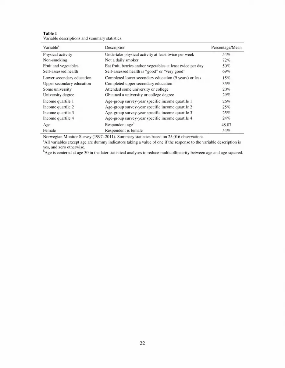
Table 1 provides the descriptions and sample means for the outcome and explanatory

variables of this study. Approximately 54% of the respondents exercise at least twice per

week, 72% are non-smokers, 50% eat fruit and vegetables at least twice per day and 69%

report their health status as either “good” or “very good”.

<< Table 1 about here >>

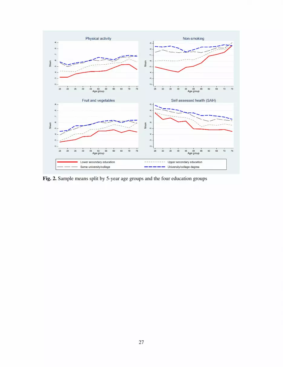
<< Fig. 1 and 2 about here >>

Fig. 1 and 2 depict age variation in lifestyles and SAH by income and education,

respectively. The figures illustrate the development in sample means for physical activity,

non-smoking, consumption of fruit and vegetables and SAH for each income quartile and

each education group at each 5-year age interval. The figures indicate that lifestyle habits

1 We thereby add 1,804 observations to the physical activity model, 1,381 observations to the non-smoking model, 619 observations to the fruit and vegetables model and 1,679 observations to the SAH model compared to the models in the results section, which all include 25,016 observations.

9

become healthier with increasing age until at least late midlife, while SAH is decreasing in

age. There are clear income and education gradients in lifestyles and SAH in most age groups.

The main exceptions are the small income gradients in lifestyles at age 25–29 years and the

small income and education gradients in non-smoking at age 75–79 years. Age variation in

the gradients are most evident in the case of income and SAH, with the gradient clearly

peaking at age 55–59 years, and in the case of education and non-smoking, with the gradient

clearly declining with higher age.

3.2. Logistic regression models

Table 2 reports the results of the income models for physical activity, non-smoking,

consumption of fruit and vegetables and SAH, and Table 3 reports the results of the

corresponding education models. The tables show odds ratios (ORs) and indicate the

significance of different ORs using asterisks.

<< Table 2 and 3 about here >>

Table 2 shows that at 30 years of age, there are clear income gradients in all outcome

variables except consumption of fruit and vegetables, and Table 3 shows that there are clear

education gradients in all outcome variables – and in particular non-smoking – at this age

(recall that the age variable is centered at 30 years of age). Thus, the results in Table 2 and 3

confirm the patterns observed in Fig. 1 and 2 with respect to the income and education

gradients in lifestyles and SAH in young adulthood.

The SAH models in the rightmost column of Table 2 and 3 suggest that SAH is

significantly associated with all three lifestyle choices, and in particular physical activity and

non-smoking. Furthermore, comparing the two SAH models in Table 2, the education

gradient in SAH becomes smaller once we control for lifestyles (e.g., the OR of university

degree is reduced from 1.88 to 1.61 when we add lifestyles as control variables). Similarly,

10

Table 3 shows that also the income gradient in SAH becomes smaller once we control for

lifestyles.2 The cross-sectional nature of our data do not allow for any casual inference.

However, these results indicate, at least, that our lifestyle indicators might be important in

affecting health (World Health Organization, 2003), and in mediating the relationship

between socioeconomic status and health (Cutler et al., 2011).

3.2. Predicted income and education gradients

Our main interest is to explore how the income and education gradients in lifestyles and

health vary with age. To facilitate interpretation, we will in the following focus mainly on

comparing results across the lowest and the highest income and education groups, and focus

less on results for the two intermediate income and education groups.

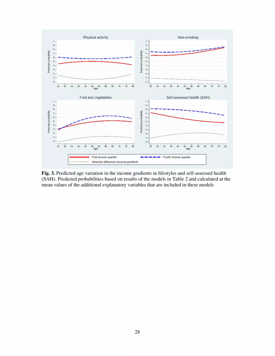
Fig. 3 is based on the results of the first four income models in Table 2 and shows how

the predicted probabilities for healthy lifestyles and good health vary with age for people in

the first and the fourth income quartiles. The figure also shows the absolute differences in

predicted probabilities between these two income groups, which we refer to as the income

gradient. The predictions were calculated at the mean values of the other explanatory

variables that are included in the models (i.e., variables that do not involve age and income).

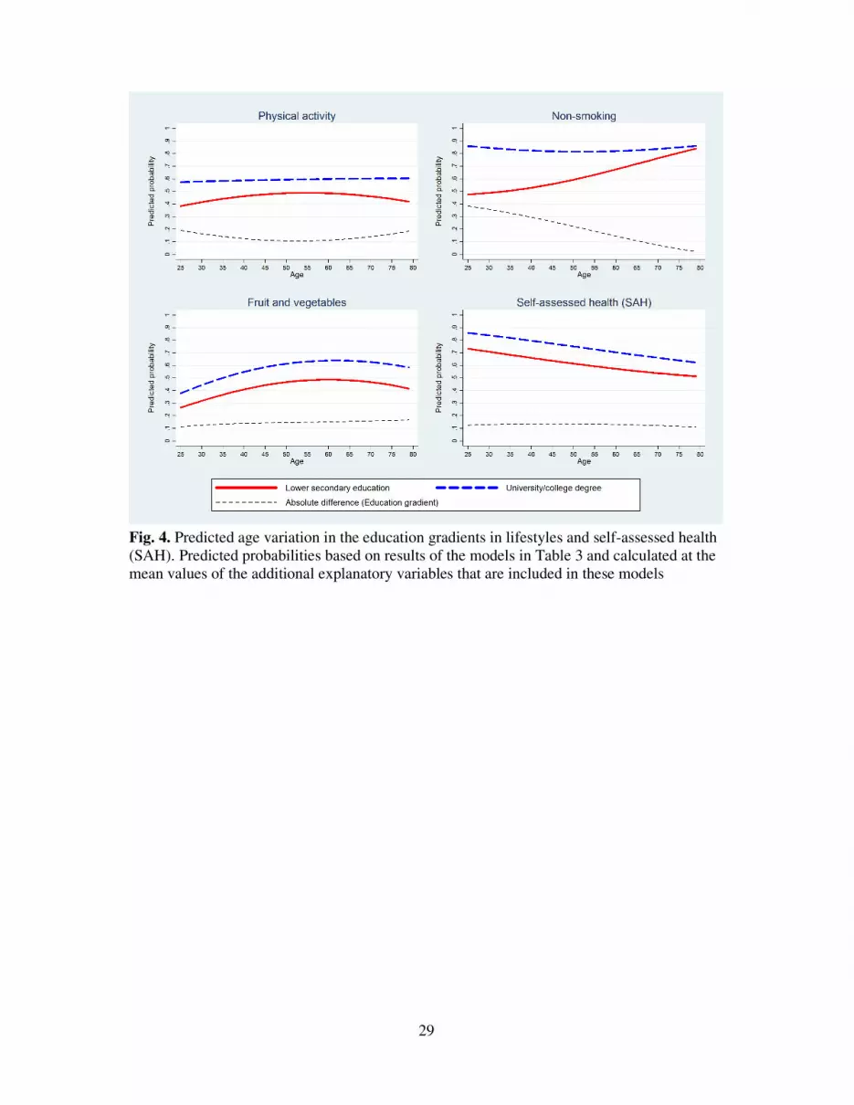
Similarly, Fig. 4 is based on the results of the first four education models in Table 3 and

shows how the predicted probabilities for healthy lifestyles and good health vary with age for

people who have completed only lower secondary education or less and for those with a

university degree, along with the absolute differences in predicted probabilities between these

two education groups, which we refer to as the education gradient.

<< Fig. 3 about here >>

2 We find similar patterns when we instead estimate the lifestyle models with current SAH added as explanatory variable. That is, all three lifestyle choices are positively associated with SAH (P < 0.01), and the income and education gradients in all three lifestyle choices become smaller once we control for SAH.

11

Fig. 3 shows that the income gradients in consumption of fruit and vegetables and

SAH are concave in age, i.e., income differences are stronger during late midlife – and at their

strongest at 60 and 61 years of age, respectively – than at younger and older ages. Table 2

shows that this age variation (Age × Income quartile 4 and Age2 × Income quartile 4) is

statistically significant at the 95% level. The strongest predicted income gradient across the

four outcome variables is found in SAH at 61 years of age, where only 52.3% of those in the

first income quartile are predicted to report being in good or very good health, compared with

75.0% of those in the fourth income quartile. As discussed, the age pattern of cumulative

advantage effects in SAH by income until late midlife followed by age-as-leveler effects at

older ages have been reported in several earlier studies (Beckett, 2000; Huijts et al., 2010; van

Kippersluis et al., 2010).

The income gradient in physical activity is convex in age, and this age variation is

statistically significant, i.e., income differences in physical activity are smaller during midlife

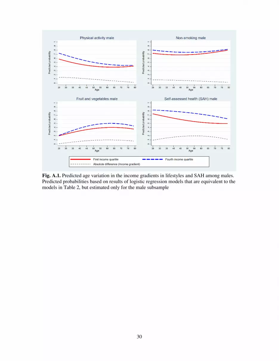
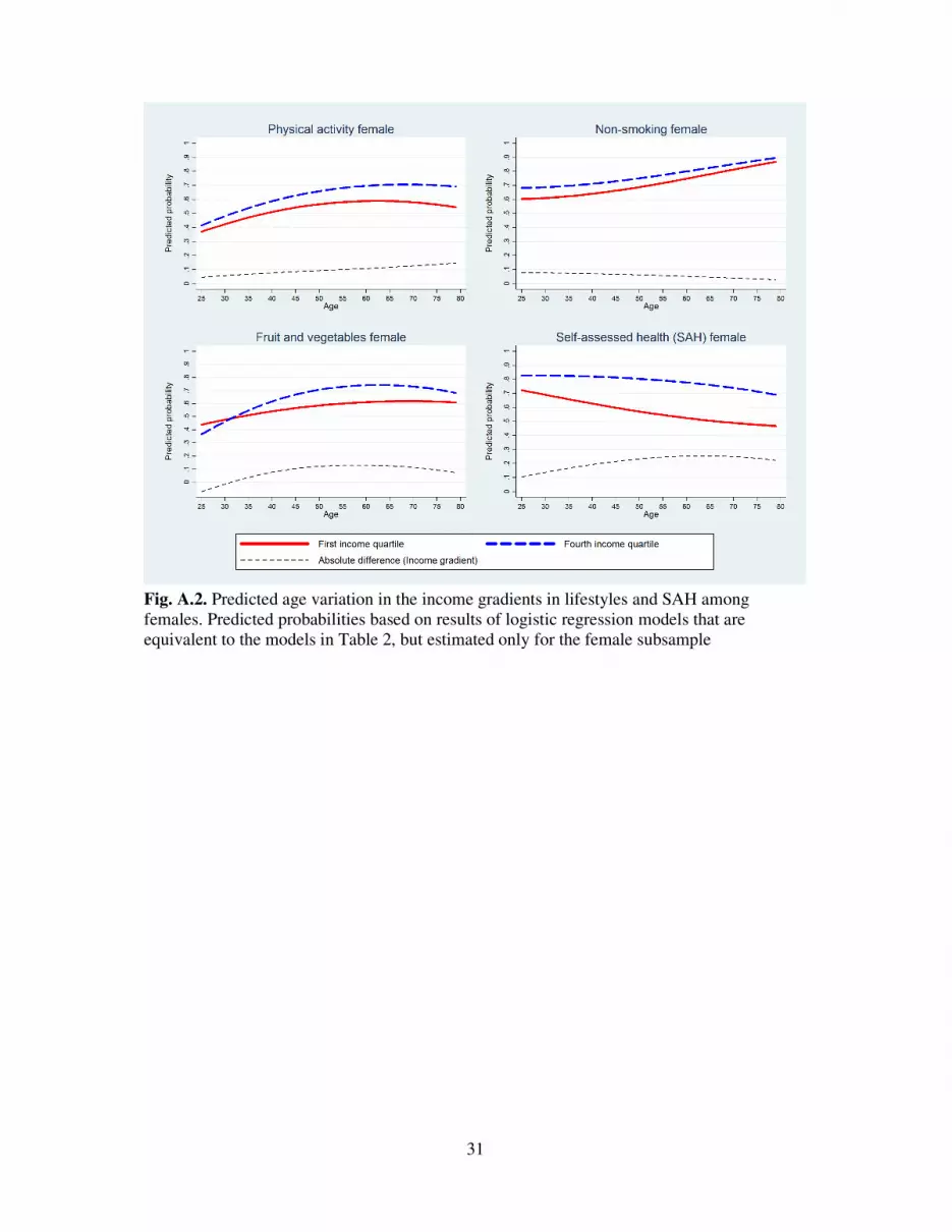
than at younger and older ages. However, this result seems to reflect gender differences; when

we estimate the models separately by gender, the income gradient in physical activity is

decreasing linearly in age among males (P < 0.05) and increasing linearly in age among

females (P < 0.10). Fig. A.1–A.4 in the Appendix are based on these gender specific models

and show how the predicted income and education gradients vary with age separately for

males and females. Finally, while Fig. 3 suggests that the income gradient in non-smoking is

decreasing somewhat in age, Table 2 shows that this age variation is not statistically

significant.

<< Fig. 4 about here >>

Table 3 shows that the education gradient in non-smoking decreases significantly and

linearly in age, and Fig. 4 shows that it moves from being very steep at young ages to almost

zero at older ages. According to our model predictions, at 25 years of age those with a

12

university or college degree are thirty-eight percentage points more likely than those who

have only completed lower secondary education or less to be non-smokers, while at 79 years

of age this difference in predicted probabilities is reduced to only two percentage points.

The education gradients in physical activity, consumption of fruit and vegetables and

SAH do not vary significantly with age, as shown in Table 2 and reflected in Fig. 4. However,

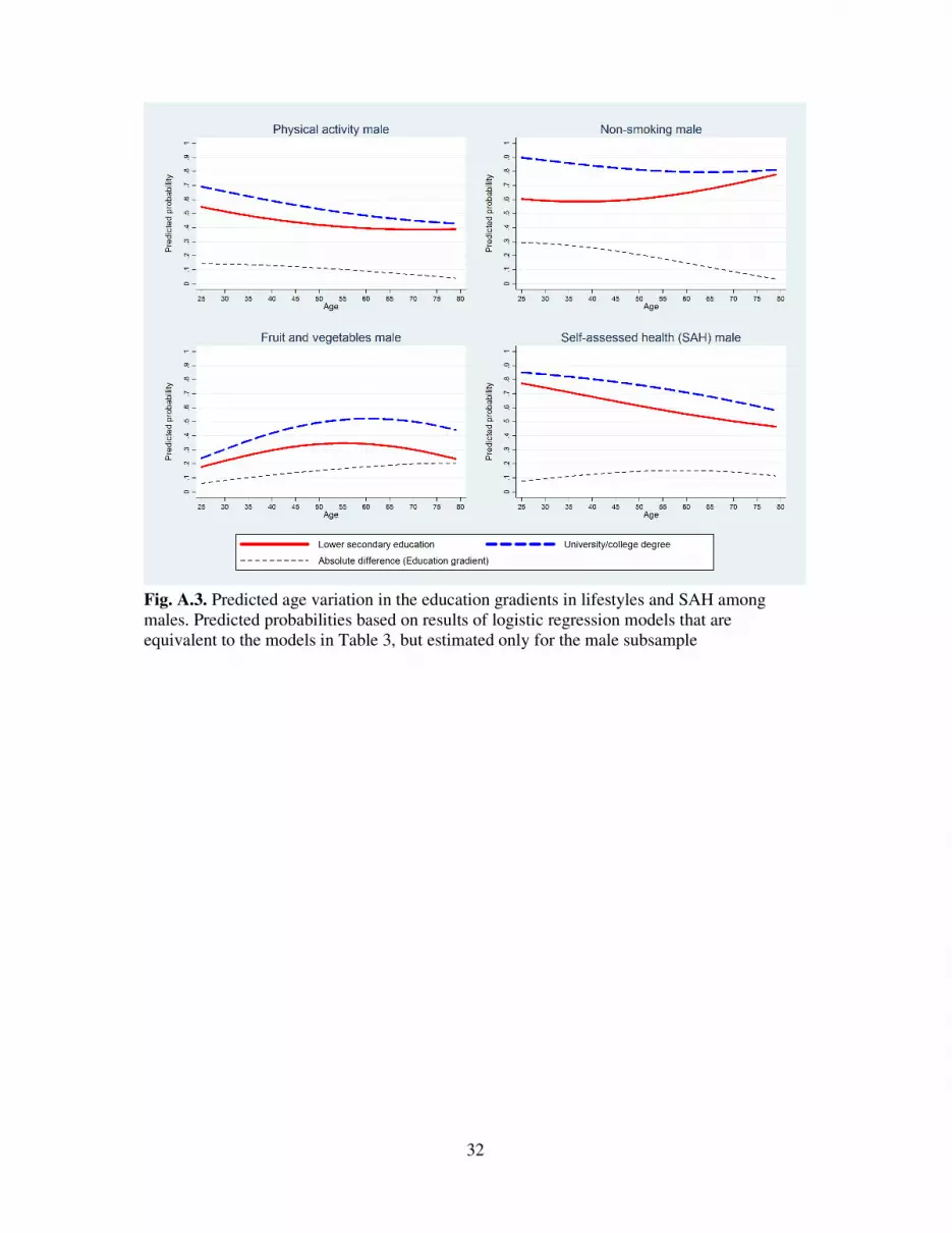
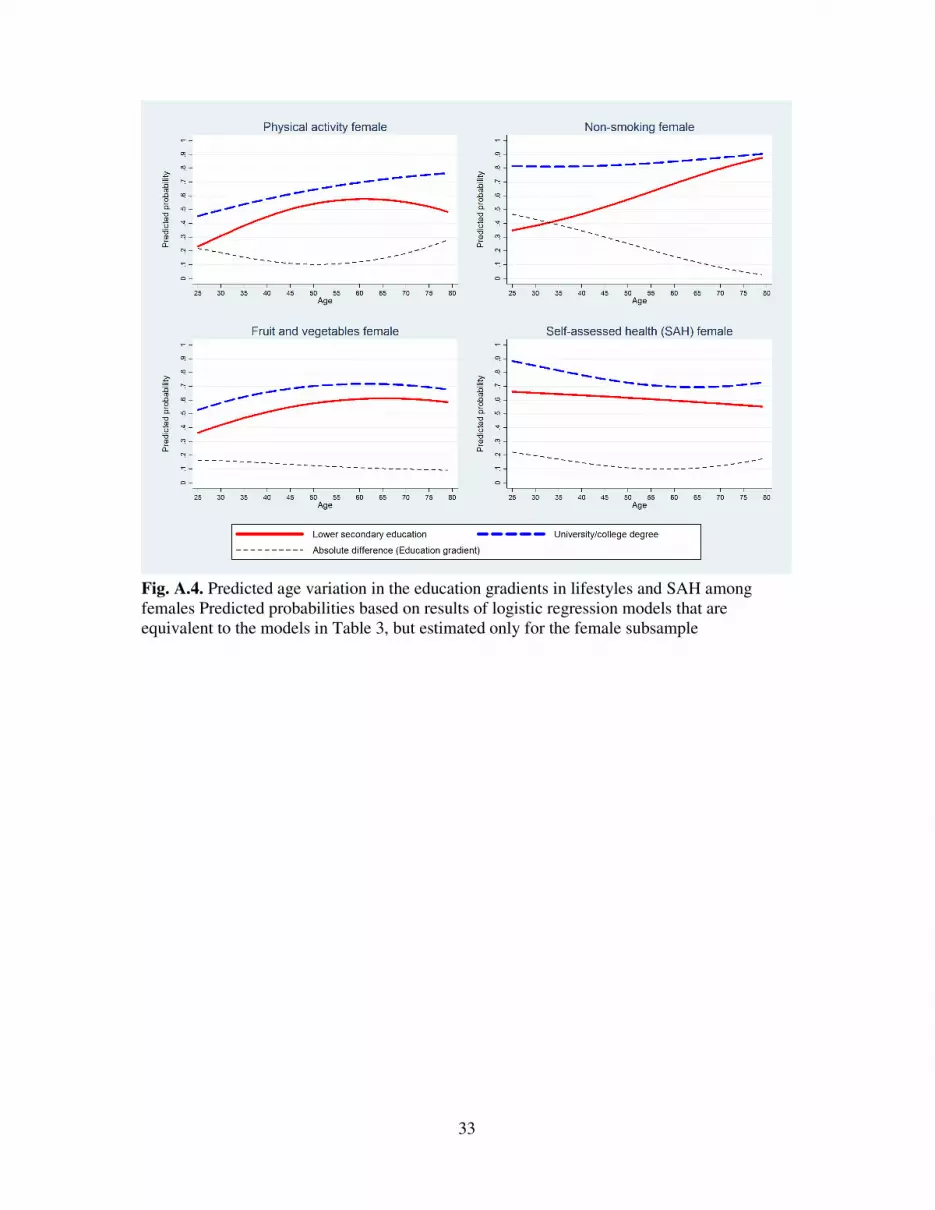
when we estimate the models separately by gender, we find that while the education gradients

in physical activity and SAH do not vary significantly with age among males, they are convex

in age among females, i.e., the education gradients in these variables among females are

smaller during late midlife – and at their smallest at 51 and 58 years of age, respectively –

than at younger and older ages (see Fig. A.4 in the Appendix).

<< Table 4 about here >>

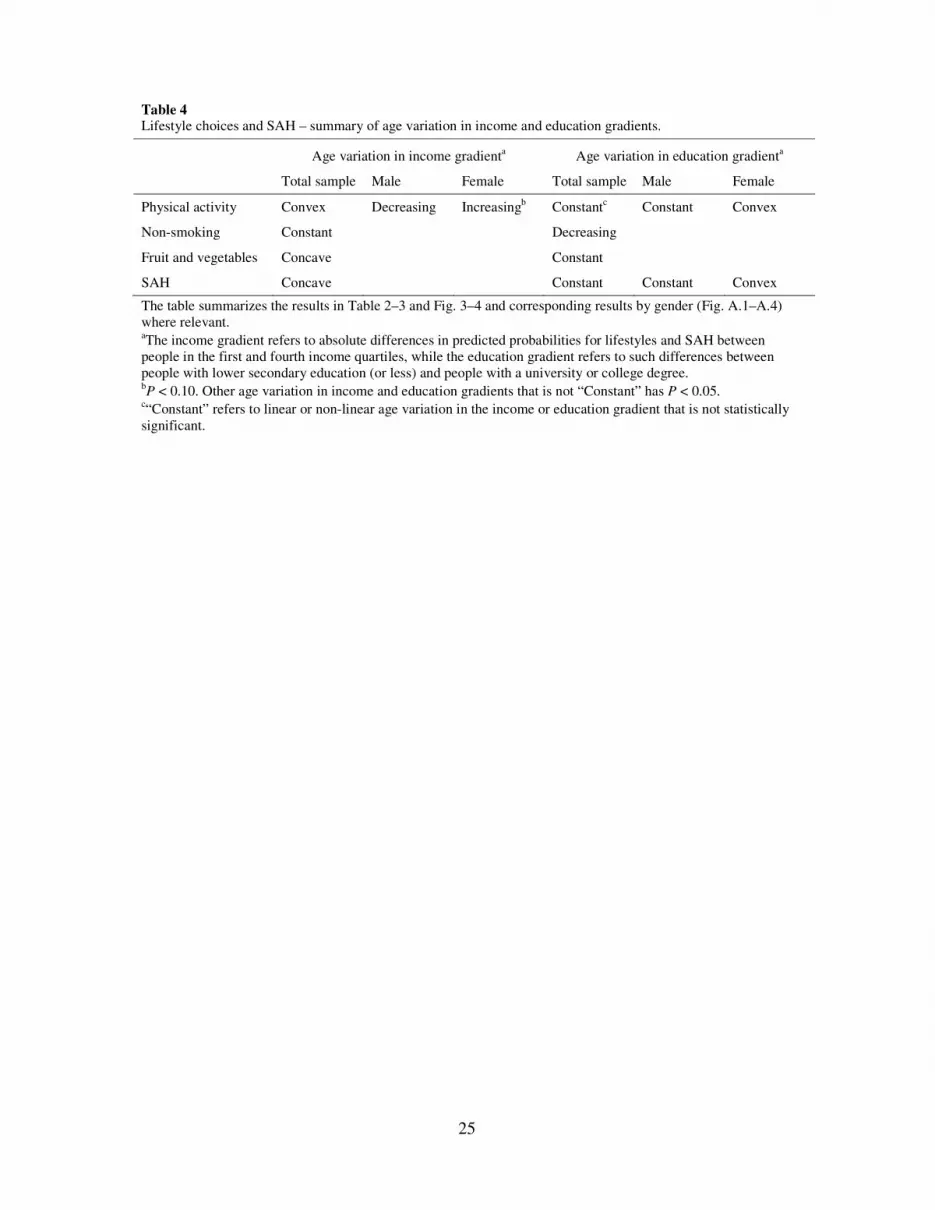
We summarize our results in Table 4. Based on the above statistical and graphical

analysis, we indicate how the income and education gradients in physical activity, non-

smoking, consumption of fruit and vegetables and SAH vary with age, including whether this

age variation is statistically significant. We separate the results by gender where relevant.

4. Discussion

The relationship between socioeconomic status and health is dynamic and may vary with age.

Our analysis has explored the potential role of lifestyle choices in explaining some of these

dynamics. We find that in Norway, there are clear income and education gradients in the

probability of being physically active, smoking and eating fruit and vegetables throughout

most stages of the adult life course. However, the predicted age patterns of inequality are

found to vary across different lifestyle choices, education and income, and to some extent

gender (see Table 4).

13

The income gradient in smoking, the education gradient in consumption of fruit and

vegetables and the education gradient in physical activity among males do not vary

significantly with age. These results suggest that lifestyle choices are expected to contribute to

cumulative advantage effects in health by socioeconomic status (Benzeval et al., 2011; Kim &

Durden, 2007; Ross & Wu, 1996; Wilson et al., 2007); throughout the life course,

socioeconomic status is closely associated with our daily investments into the production of

poor and good health. Because many adverse health outcomes are the result of long-term,

cumulative processes (Kuh & Shlomo, 2004), these daily health investments eventually result

in a relatively more rapid deterioration of health among lower than higher socioeconomic

status groups.

The education gradient in smoking, the income gradient in consumption of fruit and

vegetables and the income gradient in physical activity among males become smaller as

people grow older. These results suggest that, in some cases, the income and education

gradients in lifestyle choices may not be constant, but vary with age. To the extent that

lifestyle habits are converging with older age, as found in these examples, this may contribute

to patterns of age-as-leveler effects in health (Beckett, 2000; Huijts et al., 2010; van

Kippersluis et al., 2010), persistent health inequalities (Ferraro & Farmer, 1996), or a slowing

down of cumulative advantage effects in health by socioeconomic status at older ages.

Our analysis is based on repeated cross-sectional data, and thus we are not able to

directly assess whether converging lifestyle habits in age contribute to a slowing down of

cumulative advantage effects in health by socioeconomic status. We find that current lifestyle

choices are significantly associated with the probability of reporting good health, as

represented by SAH, and that the income and education gradients in SAH become smaller

once we control for these lifestyle indicators. We further find patterns of age-as-leveler effects

in SAH by income, persistent inequalities in SAH by education among males, and after

14

decreasing until late midlife, cumulative advantage effects in SAH by education among

females after 58 years of age.

As noted, our results are relatively mixed across different lifestyle choices, education

and income, and to some extent gender. For example, while the education gradient in physical

activity and consumption of fruit and vegetables for the total sample do not vary significantly

with age, the education gradient in non-smoking moves from being very strong at younger

ages, to almost zero at older ages. This age pattern in smoking appears too pronounced to be

explained fully by sample selection because of high mortality rates among people in the lower

education groups (Beckett, 2000). Instead, different age patterns for the above education

gradients might in part reflect systematic variation across different lifestyle choices in terms

of perceived health risks. That is, people with low levels of formal education quit smoking at

faster rates as they grow older because they learn that not doing so can seriously damage their

health (Gandini et al., 2008). While eating fruit and vegetables and being physically active are

also clearly associated with good health outcomes (Word Health Organization, 2003; He et

al., 2007; Jeon et al., 2007), this evidence may be less accessible or perceived as less striking

than the corresponding evidence on smoking (Sanderson et al., 2009).

Physical activity among females is the only lifestyle indicator for which income and

education differences are increasing in age; the income gradient increases linearly in age and

the education gradient is convex in age and at its smallest at 51 years of age. This result could

reflect the effect of time constraints as a result of combining a career with raising children

during the earlier stages of the adult life course (Sørensen & Gill, 2008). These time

constraints may be particularly pronounced among women in the highest socioeconomic

status groups. For example, studies from the USA find that both number of working hours in

the labor market and time spent with the children increases markedly with length of education

(Aguiar & Hurst, 2007; Guryan et al., 2008), which leaves less hours available for time-

15

consuming leisure activities such as physical activity (Welch et al., 2009). Thus, income and

education differences in physical activity among females may be smaller until about 50 years

of age, when time constraints are likely to be important, particularly among higher

socioeconomic status women, than at older ages, when time constraints are likely to become

increasingly less important.

To some extent, our results are sensitive to choice of education or income as

socioeconomic status indicator. While education and income are usually highly correlated,

previous life course studies have shed light on some of the fundamental differences between

these two leading socioeconomic status indicators (Cutler et al., 2011). For example, while

education is more or less fixed at an early stage of the adult life course, income may be

affected by many factors throughout the adult life course, including health shocks and the

gradual deterioration of health in age (Smith, 2004). We find, for example, that while the

income gradient in SAH is clearly peaking around pre-retirement (50–60 years of age), this is

not the case for the education gradient in SAH. According to previous studies that find similar

patterns of results, the income gradient in SAH peaks around pre-retirement mostly because

of the effect of poor health on premature exit from the labor force, which in turn negatively

affect incomes because of the shift from wage earning to a reliance on social security

payments (van Kippersluis et al., 2010).

We find that there are strong education and income gradients in lifestyles and health in

Norway, which is considered an egalitarian country, with a strong, well-funded welfare state

and a low level of income inequality (OECD, 2011). However, this result is not surprising

considering that similar results have been found in several other studies from Norway and

other Scandinavian countries (e.g., Mackenbach et al., 2008; Huijts et al., 2010; Shkolnikov et

al., 2012). While strong welfare states may not be sufficient to avoid socioeconomic

inequalities in health, it may influence the way in which such inequalities evolve over the life

16

course. For example, Lundberg et al. (2008) found that countries with generous basic security

pension systems, including Norway, experience lower rates of excess mortality among elderly

people than other countries. However, in general, the evidence on the role of social policies

and different types of welfare states in shaping life course patterns of health inequalities is

scarce (Corna, 2013), and thus more studies that address this issue are needed.

The results of this study must be considered in light of its limitations. In particular, our

analysis employs repeated cross-sectional data, and thus we are not able to fully capture the

dynamic nature of health production, nor are we able to capture possible feedbacks between

socioeconomic status, lifestyle choices and health. Thus, the results of this study are mainly of

a descriptive nature, since our data do not allow for any causal inference. Some of our key

variables may also include measurement error because of incompleteness and the reliance on

self-reported data, although, for example, SAH has been shown to be highly correlated with

several objective health measures (Idler & Benyamini, 1997). Biases may also arise from

mortality selection, as discussed, and from the fact that 10.9% of the respondents were

excluded from our final sample because of missing information on one or more relevant

variables.

Factors such as mortality selection (Beckett, 2000), the increasing importance of

biological factors relative to socioeconomic status in determining health at older ages (Herd,

2006), cohort effects (Lynch, 2003) and labor market participation status (Case & Deaton,

2005) may all be important in explaining why we sometimes observe that socioeconomic

inequalities do not continue to widen, or accumulate, into older age. However, our results

suggest that also dynamics in the relationship between socioeconomic status and health

affecting lifestyle choices may be important in explaining such patterns. Given the results and

limitations of this study, there is a need for more similar research. Studies based on long panel

data that track important lifestyle and health indicators as well as socioeconomic status in the

17

same individuals over most stages of the adult life course would be particularly relevant.

Studies on other lifestyle indicators, such as alcohol use and the consumption of unhealthy

foods, would also be interesting, as would further analyses of the three lifestyle indicators

used in this study, but possibly using alternative variable definitions (e.g., physical activity

accounting for intensity level).

Our results suggest that, except for physical activity among females, income and

education gradients in lifestyle choices either remain constant in age or become smaller with

older age. While policies for reducing health inequalities and its sources are important at all

stages of the life course, from birth to old age, policies for improved lifestyle habits may

benefit especially from targeting young people, and particularly young people with low levels

of income and formal education. Health information policies aimed towards making people

more health consciousness at younger ages may be efficient. This type of health information

could focus on the long-term, cumulative nature of health production and thus the importance

of making healthy lifestyle choices already at younger ages.

Acknowledgements

Funding for this research was provided by the Research Council of Norway, Grant Nos.

182289 and 184809. We thank two anonymous reviewers for their helpful comments and

suggestions.

References

Aguiar, M., & Hurst, E. (2007). Measuring trends in leisure: The allocation of time over five

decades. The Quarterly Journal of Economics, 122, 969–1006.

Beckett, M. (2000). Converging health inequalities in later life: an artifact of mortality

selection? Journal of Health and Social Behavior, 41, 106–119.

18

Benzeval M., Green, M. J., & Leyland, A. H. (2011). Do social inequalities in health widen or

converge with age? Longitudinal evidence from three cohorts in the West of Scotland.

BMC Public Health, 11, 947.

Case, A., & Deaton, A. (2005). Broken down by work and sex: how our health declines. In D.

A. Wise (Ed.), Analyses in the economics of aging (pp. 185–205). Chicago: Chicago

University Press.

Corna, L. M. (2013). A life course perspective on socioeconomic inequalities in health: A

critical review of conceptual frameworks. Advances in Life Course Research, 18, 150–

159.

Cutler, D. M., & Lleras-Muney, A. (2010). Understanding differences in health behaviors by

education. Journal of health economics, 29, 1–28.

Cutler, D. M., Lleras-Muney, A., & Vogl, T. (2011). Socioeconomic status and health:

dimensions and mechanisms. In: S. Glies, & P.C. Smith (Eds.), The Oxford Handbook

of Health Economics (pp. 124–163). Oxford: Oxford University Press.

Deaton, A. (1997). The analysis of Household Surveys: a Microeconometric Approach to

Development Policy (World Bank). Baltimore: The Johns Hopkins University Press.

Ferraro, K. F., & Farmer, M. M. (1996). Double jeopardy, aging as leveller, or persistent

health inequality? A longitudinal analysis of white and black Americans. Journal of

Gerontology, 51B, S319–S328.

Gandini, S., Botteri, E., Iodice, S., Boniol, M., Lowenfels, A. B., Maisonneuve, P., & Boyle,

P. (2008). Tobacco smoking and cancer: A meta‐analysis. International journal of

cancer, 122, 155–164.

Guryan, J., Hurst, E., & Kearney, M. (2008). Parental Education and Parental Time with

Children. The Journal of Economic Perspectives, 22, 23–46.

19

He, F. J., Nowson, C. A., Lucas, M., & MacGregor, G. A. (2007). Increased consumption of

fruit and vegetables is related to a reduced risk of coronary heart disease: meta-

analysis of cohort studies. Journal of human hypertension, 21, 717–728.

Herd, P. (2006). Do functional health inequalities decrease in old age? Educational status and

functional decline among the 1931-1941 birth cohort. Research on Aging, 28, 375–

392.

Huijts, T., Eikemo, T. A., & Skalická, V. (2010). Income-related health inequalities in the

Nordic countries: examining the role of education, occupational class and age. Social

Science & Medicine, 71, 1964–1972.

Idler, E. L., & Benyamini, Y. (1997). Self-rated health and mortality: a review of twenty-

seven community studies. Journal of Health and Social Behavior, 38, 21–37.

Jeon, C. Y., Lokken, R. P., Hu, F. B., & Van Dam, R. M. (2007). Physical activity of

moderate intensity and risk of type 2 diabetes: a systematic review. Diabetes Care, 30,

744–752.

Kim, J., & Durden, K. (2007). Socioeconomic status and age trajectories of health. Social

Science & Medicine, 65, 2489–2502.

van Kippersluis, H., O’Donnell, O., van Doorslaer, E., & van Ourti, T. (2010). Socioeconomic

differences in health over the life cycle in an egalitarian country. Social Science &

Medicine, 70, 428–438.

Kuh, D., & Shlomo, Y. B. (Eds.). (2004). A life course approach to chronic disease

epidemiology (Vol. 2). Oxford: Oxford University Press.

Lundberg, O., Yngwe, M. Å., Stjärne, M. K., Elstad, J. I., Ferrarini, T., Kangas, O., Norström,

T., Palme, J., & Fritzell, J. (2008). The role of welfare state principles and generosity

in social policy programmes for public health: an international comparative study. The

Lancet, 372, 1633–1640.

20

Lynch, S. M. (2003). Cohort and life course patterns in the relationship between education

and health: a hierarchical approach. Demography, 40, 309–331.

Mackenbach, J. P., Stirbu, I., Roskam, A. J. R., Schaap, M. M., Menvielle, G., Leinsalu, M.,

& Kunst, A. E. (2008). Socioeconomic inequalities in health in 22 European

countries. New England Journal of Medicine, 358, 2468–2481.

Marmot, M., Friel, S., Bell, R., Houweling, T. A., & Taylor, S. (2008). Closing the gap in a

generation: health equity through action on the social determinants of health. The

Lancet, 372, 1661–1669.

O’Brien, R. M., Hudson, K., & Stockard, J. (2008). A mixed model estimation of age, period,

and cohort effects. Sociological Methods Research, 36, 402–442.

OECD (2008). Growing unequal? Income distribution and poverty in OECD countries. Paris:

OECD Publishing.

OECD (2011). Society at a glance 2011 – OECD social indicators. Paris: OECD Publishing.

Pampel, F. C., Krueger, P. M., & Denney, J. T. (2010). Socioeconomic disparities in health

behaviors. Annual review of sociology, 36, 349.

Reither, E. N., Hauser, R. M., & Yang, Y. (2009). Do birth cohorts matter? Age–period–

cohort analyses of the obesity epidemic in the United States. Social Science &

Medicine, 69, 1439–1448.

Ross, C. E., & Wu, C. L. (1996). Education, age, and the cumulative advantage in health.

Journal of Health and Social Behavior, 37, 104–120.

Sanderson, S. C., Waller, J., Jarvis, M. J., Humphries, S. E., & Wardle, J. (2009). Awareness

of lifestyle risk factors for cancer and heart disease among adults in the UK. Patient

Education and Counseling, 74, 221–227.

21

Sarma, S., Thind, A., & Chu, M. (2011). Do new cohorts of family physicians work less

compared to their older predecessors? The evidence from Canada. Social Science &

Medicine, 72, 2049–2058.

Shkolnikov, V. M., Andreev, E. M., Jdanov, D. A., Jasilionis, D., Kravdal, Ø., Vågerö, D., &

Valkonen, T. (2012). Increasing absolute mortality disparities by education in Finland,

Norway and Sweden, 1971–2000. Journal of epidemiology and community health, 66,

372–378.

Sofi, F., Capalbo, A., Cesari, F., Abbate, R., & Gensini, G. F. (2008). Physical activity during

leisure time and primary prevention of coronary heart disease: an updated meta-

analysis of cohort studies. European Journal of Cardiovascular Prevention &

Rehabilitation, 15, 247–257.

Smith, J. P. (2004). Unraveling the SES: health connection. Population and Development

Review, 30, 108–132.

Sørensen, M., & Gill, D. L. (2008). Perceived barriers to physical activity across Norwegian

adult age groups, gender and stages of change. Scandinavian Journal of Medicine &

Science in Sports, 18, 651–663.

Welch, N., McNaughton, S. A., Hunter, W., Hume, C., & Crawford, D. (2009). Is the

perception of time pressure a barrier to healthy eating and physical activity among

women? Public health nutrition, 12, 888–895.

Wilson, A., Shuey, K., & Elder, G. (2007). Cumulative advantage processes as mechanisms

of inequality in life course health. American Journal of Sociology, 112, 1886–1924.

World Health Organization (2003). Diet, nutrition and the prevention of chronic diseases.

WHO Technical Report Series No. 916, Geneva, Switzerland.

22

Table 1 Variable descriptions and summary statistics.

Variablea Description Percentage/Mean

Physical activity Undertake physical activity at least twice per week 54% Non-smoking Not a daily smoker 72% Fruit and vegetables Eat fruit, berries and/or vegetables at least twice per day 50% Self-assessed health Self-assessed health is “good” or “very good” 69%

Lower secondary education Completed lower secondary education (9 years) or less 15% Upper secondary education Completed upper secondary education 35% Some university Attended some university or college 20% University degree Obtained a university or college degree 29%

Income quartile 1 Age-group survey-year specific income quartile 1 26% Income quartile 2 Age-group survey-year specific income quartile 2 25% Income quartile 3 Age-group survey-year specific income quartile 3 25% Income quartile 4 Age-group survey-year specific income quartile 4 24%

Age Respondent ageb 48.07 Female Respondent is female 54% Norwegian Monitor Survey (1997–2011). Summary statistics based on 25,016 observations. aAll variables except age are dummy indicators taking a value of one if the response to the variable description is yes, and zero otherwise. bAge is centered at age 30 in the later statistical analyses to reduce multicollinearity between age and age-squared.

23

Table 2 Logistic regressions for lifestyle choices and health – income models.

Physical activity

Non- smoking

Fruit and vegetables

Self-assessed health (SAH)

Self-assessed health (SAH)

OR OR OR OR OR

Agea 1.17 0.98 1.47*** 0.73** 0.69*** Age2 0.96** 1.05*** 0.95*** 1.03 1.03

Income quartile 2b 1.19** 1.26*** 1.05 1.60*** 1.55*** Income quartile 2 × Age 0.85* 1.02 1.15 0.98 1.00 Income quartile 2 × Age2 1.05** –c 0.97 1.00 1.00

Income quartile 3 1.39*** 1.38*** 1.11 1.83*** 1.74*** Income quartile 3 × Age 0.92 1.00 1.19* 1.11 1.10 Income quartile 3 × Age2 1.02 –c 0.97 0.98 0.98

Income quartile 4 1.68*** 1.49*** 1.07 2.01*** 1.85*** Income quartile 4 × Age 0.77*** 0.95 1.34*** 1.29** 1.31** Income quartile 4 × Age2 1.07*** –c 0.95** 0.95** 0.95**

Female 1.33*** 0.93** 2.73*** 1.03 0.97 Upper secondary educationb 1.21*** 1.26*** 1.20*** 1.18*** 1.13** Some university 1.57*** 1.97*** 1.65*** 1.54*** 1.37*** University degree 1.71*** 3.09*** 1.86*** 1.88*** 1.61***

Physical activity 1.63*** Non-smoking 1.57*** Fruit and vegetables 1.11*** Norwegian Monitor Survey (1997–2011). All models based on 25,016 observations. a Age and Age2 have been centered at age 30 and divided by 10 and 102, respectively. b Income quartile 1 and Lower secondary education are the reference groups. c No Age2 × Income-interactions had P < 0.05 and were removed from the final model. OR odds ratio. *P < 0.10; **P < 0.05; ***P < 0.01.

24

Table 3 Logistic regressions for lifestyle choices and health – education models.

Physical activity

Non-smoking

Fruit and vegetables

Self-assessed health (SAH)

Self-assessed health (SAH)

OR OR OR OR OR

Agea 1.27 1.12 1.60*** 0.79** 0.74*** Age2 0.95* 1.05*** 0.92*** 1.01 1.02

Upper secondary educationb 1.31* 1.71*** 1.04 1.18 1.09 Upper secondary education × Age 0.84 0.90** 1.07* 1.01 1.02 Upper secondary education × Age2 1.05* –c –c –c –c

Some university 1.90*** 3.39*** 1.50*** 1.78*** 1.49*** Some university × Age 0.74** 0.78*** 1.04 0.94 0.96 Some university × Age2 1.07** –c –c –c –c

University degree 1.94*** 5.77*** 1.71*** 2.15*** 1.72*** University degree × Age 0.82 0.72*** 1.03 0.94 0.97 University degree × Age2 1.05 –c –c –c –c

Female 1.33*** 0.91*** 2.73*** 1.02 0.97 Income quartile 2b 1.19*** 1.31*** 1.16*** 1.57*** 1.51*** Income quartile 3 1.31*** 1.39*** 1.30*** 1.95*** 1.86*** Income quartile 4 1.48*** 1.39*** 1.41*** 2.49*** 2.35***

Physical activity 1.63*** Non-smoking 1.56*** Fruit and vegetables 1.11*** Norwegian Monitor Survey (1997–2011). All models based on 25,016 observations. a Age and Age2 have been centered at age 30 and divided by 10 and 102, respectively. b Income quartile 1 and Lower secondary education are the reference groups. c No Age2 × Education-interactions had P < 0.05 and were removed from the final model. OR odds ratio. *P < 0.10; **P < 0.05; ***P < 0.01.

25

Table 4 Lifestyle choices and SAH – summary of age variation in income and education gradients.

Age variation in income gradienta Age variation in education gradienta

Total sample Male Female Total sample Male Female

Physical activity Convex Decreasing Increasingb Constantc Constant Convex

Non-smoking Constant Decreasing

Fruit and vegetables Concave Constant

SAH Concave Constant Constant Convex

The table summarizes the results in Table 2–3 and Fig. 3–4 and corresponding results by gender (Fig. A.1–A.4) where relevant. aThe income gradient refers to absolute differences in predicted probabilities for lifestyles and SAH between people in the first and fourth income quartiles, while the education gradient refers to such differences between people with lower secondary education (or less) and people with a university or college degree. bP < 0.10. Other age variation in income and education gradients that is not “Constant” has P < 0.05.

c“Constant” refers to linear or non-linear age variation in the income or education gradient that is not statistically significant.

26

Fig. 1. Sample means split by 5-year age groups and age-group survey-year specific income quartiles

27

Fig. 2. Sample means split by 5-year age groups and the four education groups

28

Fig. 3. Predicted age variation in the income gradients in lifestyles and self-assessed health (SAH). Predicted probabilities based on results of the models in Table 2 and calculated at the mean values of the additional explanatory variables that are included in these models

29

Fig. 4. Predicted age variation in the education gradients in lifestyles and self-assessed health (SAH). Predicted probabilities based on results of the models in Table 3 and calculated at the mean values of the additional explanatory variables that are included in these models

30

Fig. A.1. Predicted age variation in the income gradients in lifestyles and SAH among males. Predicted probabilities based on results of logistic regression models that are equivalent to the models in Table 2, but estimated only for the male subsample

31

Fig. A.2. Predicted age variation in the income gradients in lifestyles and SAH among females. Predicted probabilities based on results of logistic regression models that are equivalent to the models in Table 2, but estimated only for the female subsample

32

Fig. A.3. Predicted age variation in the education gradients in lifestyles and SAH among males. Predicted probabilities based on results of logistic regression models that are equivalent to the models in Table 3, but estimated only for the male subsample

33

Fig. A.4. Predicted age variation in the education gradients in lifestyles and SAH among females Predicted probabilities based on results of logistic regression models that are equivalent to the models in Table 3, but estimated only for the female subsample