Embed Size (px)
Citation preview
LILIANA COJOCARU
Advanced Studies on the Complexity of Formal Languages
Acta Universitatis Tamperensis 2192
LILIAN
A CO
JOC
AR
U A
dvanced Studies on the C
omplexity of Form
al Languages A
UT 2192
LILIANA COJOCARU
Advanced Studies on the Complexity of Formal Languages
ACADEMIC DISSERTATIONTo be presented, with the permission of
the Board of the School of Information Sciences of the University of Tampere, for public discussion in the Väinö Linna auditorium K 104,
Kalevantie 5, Tampere, on 24 August 2016, at 12 o’clock.
UNIVERSITY OF TAMPERE
LILIANA COJOCARU
Advanced Studies on the Complexity of Formal Languages
Acta Universi tati s Tamperensi s 2192Tampere Universi ty Pres s
Tampere 2016
ACADEMIC DISSERTATIONUniversity of TampereSchool of Information Sciences Finland
Copyright ©2016 Tampere University Press and the author
Cover design byMikko Reinikka
Acta Universitatis Tamperensis 2192 Acta Electronica Universitatis Tamperensis 1691ISBN 978-952-03-0183-5 (print) ISBN 978-952-03-0184-2 (pdf )ISSN-L 1455-1616 ISSN 1456-954XISSN 1455-1616 http://tampub.uta.fi
Suomen Yliopistopaino Oy – Juvenes PrintTampere 2016 441 729
Painotuote
Distributor:[email protected]://verkkokauppa.juvenes.fi
The originality of this thesis has been checked using the Turnitin OriginalityCheck service in accordance with the quality management system of the University of Tampere.
To my parents
Declaration of Authorship
I declare that this thesis titled Advanced Studies on the Complexity of Formal Languages
has been thought and written by me, and the results presented in it are my own results.
Results by other authors have been cited accordingly.
Most of the work in this thesis has been published in [30, 31, 32, 33, 34, 36, 37, 38, 39,
40, 41, 42]. The results in Chapter 3 have been merged into the work [35], and are being
prepared for submission.
Liliana Cojocaru
ii
Abstract
Advanced Studies on the Complexity of
Formal Languagesby Liliana Cojocaru
In the fields of computer science, mathematics, statistics, (bio)physics, or in any other
science that requires mathematical approaches, complexity estimates the computational
resources needed by a device to resolve a problem. Almost in all scientific fields, compu-
tational processes are measured in terms of time (steps or elementary operations), space
(memory), circuitry (nets or hardware) and more recently communication (amount of
information).
Computational complexity theory deals with the minimum of computational resources
required by a process to carry out a certain computation. Imposing restrictions on the
resources used by a particular computational model, this theory classifies problems and
algorithms into complexity classes. Hence, a complexity class is the set of all problems
(or languages, if we properly encode a problem over an alphabet) solvable (or acceptable)
by a certain model of computation using a certain amount of resources.
This dissertation encompasses results obtained by the author in the area of the complex-
ity of formal languages. We focus on classes of languages of low complexity, where low
complexity means sublinear resources. In general, low level complexity can be reached
via parallel computation, and therefore the main computational model used throughout
this thesis is the indexing alternating Turing machine. This “hybrid model” defines the
so called ALOGTIME complexity class, which may be considered as a binder between
circuitry, parallel, and sequential complexity classes. Other acceptors used in this the-
sis, to simulate generators in formal language theory, are sequential Turing machines,
multicounter machines, and branching programs.
The most frequently cited low level complexity classes in this thesis are DSPACE(log n)
and NSPACE(log n) (the classes of languages accepted by a deterministic and, respec-
tively, nondeterministic, sequential Turing machine usingO(log n) space), ALOGTIME,
and uniform-NC1 (the class of languages accepted by polynomial size log-space uniform
Boolean circuits, with depth O(log n) and fan-in 2).
The generative devices investigated in this dissertation are Chomsky grammars, regulated
rewriting systems, and grammar systems. Each generative device has assigned a Szilard
iii
language, which in terms of labels associated with the rules or components, describes
the derivations in the considered generator.
Chomsky grammars We prove NC1 upper bounds for the classes of unrestricted and
leftmost Szilard languages associated with Chomsky grammars. Most of them are tighter
improvements of the DSPACE(log n) bound. Additionally, we propose an alternative
proof of the Chomsky-Schutzenberger theorem, based on a graphical approach. In this
respect we introduce a new normal form for context-free grammars, called Dyck normal
form, and a transition diagram associated with derivations in context-free grammars in
Dyck normal form. Inspired from these structures we propose a new regular approxima-
tion method for context-free languages.
Regulated Rewriting Systems We investigate the complexity of unrestricted and leftmost-
like Szilard languages associated with matrix grammars, random context grammars, and
programmed grammars. We prove that the classes of unrestricted Szilard languages of
matrix grammars without appearance checking, random context grammars and pro-
grammed grammars, with or without appearance checking, can be accepted by indexing
alternating Turing machines in logarithmic time and space. The same results hold for
the classes of leftmost-1 Szilard languages of matrix grammars and programmed gram-
mars, without appearance checking, and for the class of leftmost-1 Szilard languages
of random context grammars, with or without appearance checking. All these classes
are contained in UE∗-uniform NC1. The class of unrestricted Szilard languages of ma-
trix grammars with appearance checking can be recognized by deterministic Turing
machines in O(log n) space and O(n log n) time. Consequently, all classes of Szilard lan-
guages mentioned above are contained in DSPACE(log n). The classes of leftmost-i,
i ∈ 1, 2, 3, Szilard languages of matrix, random-context, and programmed grammars
with context-free rules, with or without appearance checking, can be recognized by non-
deterministic Turing machines in O(log n) space and O(n log n) time. Consequently,
these classes of leftmost-like Szilard languages are included in NSPACE(log n).
Grammar Systems One of the most important dimension of the real life is the capacity
of communication. Communication is everywhere, expressed through the meaning of
human languages or coding systems, communication between different parts of a com-
puter, communication between agents and networks, communication in plants (cellular
communication), in chemical or physical reactions. The parallelism applied to them
will improve the communication performance, the time and space complexity, and the
amount of information exchanged during the communication process. Grammar systems
are formal devices that encompasses some of these phenomena. In this dissertation we
investigate two grammar system models, the parallel communicating grammar system
and cooperating distributed grammar system.
The communication in parallel communicating grammar systems is based on request-
response operations performed by the system components through so called query sym-
bols produced by query rules. Hence, the Szilard language associated with derivations in
these systems is a suitable structure through which the communication can be visualized
and studied. We prove that the classes of Szilard languages of returning or non-returning
centralized and non-returning non-centralized parallel communicating grammar systems
are included in UE∗-uniform NC1.
To study the communication in cooperating distributed grammar systems, working under
the classical derivation modes, we define several complexity structures (by means of
cooperation and communication Szilard languages) and two complexity measures (the
cooperation and communication complexity measures). We present trade-offs between
time, space, cooperation, and communication complexity of languages generated by these
grammar systems with regular, linear, and context-free components.
We present simulations of cooperating distributed grammar systems, working in com-
petence modes, by one-way multicounter machines and one-way partially blind multi-
counter machines. These simulations are performed in linear time and space, with a
linear-bounded number of reversals, and respectively, in quasirealtime. As main conse-
quences we reach (alternative) proofs of some decidability problems for these grammar
systems and (through their generative power) for regulated rewriting grammars and
systems. We further prove, via bounded width branching program simulations, that the
classes of Szilard languages of cooperating distributed grammar systems, working under
the classical derivation modes, are included in UE∗-uniform NC1.
Acknowledgements
First of all, I would like to express my deepest gratitude to my PhD supervisor Professor
Erkki Makinen for his continuous support and encouragement in everything we have
planned and brought to an end at the School of Information Sciences, University of
Tampere. For his patience with me over the years, for his patience and meticulosity in
handling the hundreds of drafts I sent to him for verification, for his technical and stylistic
suggestions that made my papers readable, and above all these, for his confidence in my
work. Without his guidance this work would not have been possible.
I am indebted to all people in the Computer Science Department at the University of
Tampere, who, directly or indirectly, have contributed to a pleasant working atmosphere
and unforgettable moments. Especially, I would like to thank to Professors Lauri Hella,
Kari-Jouko Raiha, Jyrki Nummenmaa, Roope Raisamo, and last but not least, to the
Dean of the School, Professor Mika Grundstrom. I thank the administrative staff who
helped me to deal with all (unavoidable) bureaucratic matters: Elisa Laatikainen, Soile
Levalahti, Tuula Mantyniemi, Minna Parviainen, and Kirsi Tuominen.
I am very grateful to the University of Tampere and the School of Information Sciences
for all the financial support granted to me, which made possible my productive PhD
research.
“Trees must develop deep roots in order to grow strong and produce their beauty.” I
have many roots and I am deeply grateful to all who contributed to my (scientific)
formation. I am very grateful to Professor Erzsebet Csuhaj-Varju for introducing me
into the field of grammar systems. I would like to thank her and Professor Gyorgy Vaszil
for giving me the opportunity to have a research stay at the Computer and Automation
Research Institute of the Hungarian Academy of Sciences, for all scientific discussions
we had in Budapest and in Tarragona. I am also grateful to Professor Jurgen Dassow
for introducing me into the field of regulated grammars, for the research stay he offered
me at Otto-von-Guericke University of Magdeburg. I would like to thank Professor
Juraj Hromkovic for the opportunity he gave me to visit the Swiss Federal Institute
of Technology in Zurich, Department of Information Technologies and Education. The
plan was to finalize a paper on the communication complexity of grammar systems. The
other (unplanned) papers were merely the product of the challenging discussions we had
on the complexity of grammar systems.
I would also like to express my warmest gratitude to Professor Ferucio Laurentiu Tiplea,
Alexandru Ioan Cuza University of Iasi, for his constant encouragement, for all construc-
tive discussions we had regarding my papers and my research work in computational
vi
and complexity theory, for the opportunity he gave me to conduct some of his seminars,
and for his confidence in me. I hope I did not disappoint him.
Once in my life I spent (good and productive) times at Rovira i Virgili University of
Tarragona, inside the PhD School in Formal Languages and Applications, developed by
Professor Carlos Martın-Vide. We were too many for him to take care of thoroughly,
and therefore some of us decided to make their own way. But now, looking back into
the past, I may say that this place was like a Mecca for me. Great place and great
people from all around the world. I could not have reached my current scientific level if
I had not had the chance to attend the lectures of the PhD School in Formal Languages
and Applications at Rovira i Virgili University. Therefore, I wish to express my sincere
thanks to all professors who have been involved in this program, especially to those I had
the opportunity to share some ideas: Professors Erzsebet Csuhaj-Varju, Jurgen Dassow,
Hendrik Jan Hoogeboom, Tero Harju, Henning Bordihn, Markus Holzer, Carlos Martın-
Vide, Victor Mitrana, Gheorghe Paun, Masami Ito, Juhani Karhumaki, Jarkko Kari,
Jetty Kleijn, Zoltan Esik, Gemma Bel Enguix, Maria Dolores Jimenez Lopez, Jean-Eric
Pin, Kai Salomaa, Valtteri Niemi, and Detlef Wotschke.
I have to confess that many passages in my PhD thesis are the product of many brain-
storming discussions I had with my supervisor Prof. Erkki Makinen (on Szilard lan-
guages), with Prof. Erzsebet Csuhaj-Varju and Prof. Jurgen Dassow (on grammar
systems), with Prof. Juraj Hromkovic (on communication complexity and multicounter
machines), with Prof. Hendrik Jan Hogeboom and Prof. Ferucio Laurentiu Tiplea (on
the complexity of context-free languages), with Prof. Henning Bordihn (on a simple
formula: Mathematics + Philosophy = Computer Science), and also with myself.
I would also like to thank the pre-examiners of my PhD thesis: Professor Henning Fernau,
University of Trier, and Professor Alexander Meduna, Brno University of Technology,
for reading my dissertation and for their constructive comments upon the manuscript. I
feel honored that Professor Galina Jiraskova, Slovak Academy of Sciences, accepted to
be the opponent in my public PhD defense.
Finally, I wish to thank Sydney Padua and Shafali Anand for the permission to use their
lovely caricatures.
Iasi, Romania, June 2016
Liliana Cojocaru
Contents
Declaration of Authorship ii
Abstract iii
Acknowledgements vi
Contents viii
1 Introduction 1
1.1 On a Simple Formula:Mathematics + Philosophy = Computer Science . . . . . . . . . . . . . . . 1
1.2 Overview and the Structure of the Thesis . . . . . . . . . . . . . . . . . . 10
2 Elements of Formal Language Theory 20
2.1 Graphs and Graph Representations . . . . . . . . . . . . . . . . . . . . . . 21
2.2 Alphabets, Words, and Languages . . . . . . . . . . . . . . . . . . . . . . 22
2.3 Chomsky Grammars . . . . . . . . . . . . . . . . . . . . . . . . . . . . . . 23
2.3.1 Grammars, Languages, and Hierarchies . . . . . . . . . . . . . . . 23
2.3.2 Szilard Languages . . . . . . . . . . . . . . . . . . . . . . . . . . . 27
2.3.3 Dyck Languages . . . . . . . . . . . . . . . . . . . . . . . . . . . . 28
2.3.4 Normal Forms . . . . . . . . . . . . . . . . . . . . . . . . . . . . . 29
2.3.5 Dyck Normal Form . . . . . . . . . . . . . . . . . . . . . . . . . . . 30
3 Homomorphic Representations and Regular Approximations of Lan-guages 36
3.1 Homomorphic Representations of Languages . . . . . . . . . . . . . . . . . 38
3.2 Further Remarks on the Structure of Context-Free Languages and Homo-morphic Representation . . . . . . . . . . . . . . . . . . . . . . . . . . . . 42
3.3 Further Refinements of the Regular Language in the Chomsky-SchutzenbergerTheorem . . . . . . . . . . . . . . . . . . . . . . . . . . . . . . . . . . . . . 51
3.4 On a Regular Superset Approximation for Context-Free Languages . . . . 58
3.5 Conclusions and Further Investigations . . . . . . . . . . . . . . . . . . . . 62
4 Asymptotic Growth, Computational Models, and Complexity Classes 64
4.1 Asymptotic Growth Ratio . . . . . . . . . . . . . . . . . . . . . . . . . . . 64
viii
Contents
4.1.1 Asymptotic Upper Bounds . . . . . . . . . . . . . . . . . . . . . . 65
4.1.2 Asymptotic Lower Bounds . . . . . . . . . . . . . . . . . . . . . . . 66
4.1.3 Asymptotic Equivalence . . . . . . . . . . . . . . . . . . . . . . . . 66
4.2 Computational Models and Complexity Classes . . . . . . . . . . . . . . . 67
4.2.1 Turing Machines . . . . . . . . . . . . . . . . . . . . . . . . . . . . 69
4.2.2 Alternating Turing Machines . . . . . . . . . . . . . . . . . . . . . 72
4.2.3 Multicounter Machines . . . . . . . . . . . . . . . . . . . . . . . . . 76
4.2.4 Boolean Circuits and the NC-classes . . . . . . . . . . . . . . . . . 79
4.2.5 Branching Programs . . . . . . . . . . . . . . . . . . . . . . . . . . 83
5 The Complexity of Szilard Languages of Chomsky Grammars 85
5.1 A Brief Survey . . . . . . . . . . . . . . . . . . . . . . . . . . . . . . . . . 85
5.2 NC1 Refinements . . . . . . . . . . . . . . . . . . . . . . . . . . . . . . . . 87
5.2.1 Szilard Languages of Context-Free Grammars . . . . . . . . . . . . 88
5.2.2 Szilard Languages of Phrase-Structure Grammars . . . . . . . . . . 90
5.3 Conclusions and Further Investigations . . . . . . . . . . . . . . . . . . . . 101
6 Regulated Rewriting Grammars and Lindenmayer Systems 102
6.1 Matrix Grammars . . . . . . . . . . . . . . . . . . . . . . . . . . . . . . . 103
6.1.1 Definitions and Notations . . . . . . . . . . . . . . . . . . . . . . . 103
6.1.2 Generative Capacity . . . . . . . . . . . . . . . . . . . . . . . . . . 106
6.1.3 On the Complexity of Szilard Languages . . . . . . . . . . . . . . . 107
6.1.4 Conclusions and Further Investigations . . . . . . . . . . . . . . . . 121
6.2 Random Context Grammars . . . . . . . . . . . . . . . . . . . . . . . . . . 122
6.2.1 Definitions and Notations . . . . . . . . . . . . . . . . . . . . . . . 122
6.2.2 Generative Capacity . . . . . . . . . . . . . . . . . . . . . . . . . . 124
6.2.3 On the Complexity of Szilard Languages . . . . . . . . . . . . . . . 125
6.2.4 Conclusions and Further Investigations . . . . . . . . . . . . . . . . 136
6.3 Programmed Grammars . . . . . . . . . . . . . . . . . . . . . . . . . . . . 137
6.3.1 Prerequisites . . . . . . . . . . . . . . . . . . . . . . . . . . . . . . 137
6.3.2 Generative Capacity . . . . . . . . . . . . . . . . . . . . . . . . . . 139
6.3.3 On the Complexity of Szilard Languages . . . . . . . . . . . . . . . 139
6.3.4 Conclusions and Further Investigations . . . . . . . . . . . . . . . . 143
6.4 Lindenmayer Systems . . . . . . . . . . . . . . . . . . . . . . . . . . . . . 144
6.4.1 Prerequisites . . . . . . . . . . . . . . . . . . . . . . . . . . . . . . 144
6.4.2 Computational Power . . . . . . . . . . . . . . . . . . . . . . . . . 145
7 Grammar Systems 147
7.1 Parallel Communicating Grammar Systems . . . . . . . . . . . . . . . . . 148
7.1.1 Prerequisites . . . . . . . . . . . . . . . . . . . . . . . . . . . . . . 148
7.1.2 Computational Power and Computational Complexity . . . . . . . 152
7.1.3 Communication Complexity of PC Grammar Systems . . . . . . . 153
7.1.4 Complexity Results for Szilard Languages of PC GrammarSystems . . . . . . . . . . . . . . . . . . . . . . . . . . . . . . . . . 157
7.1.5 Conclusions and Further Research . . . . . . . . . . . . . . . . . . 168
7.2 Cooperating Distributed Grammar Systems . . . . . . . . . . . . . . . . . 169
7.2.1 Prerequisites . . . . . . . . . . . . . . . . . . . . . . . . . . . . . . 169
Contents
7.2.2 Computational Power and Computational Complexity . . . . . . . 173
7.2.3 A Simulation of CD Grammar Systems by MulticounterMachines - Decidability Results . . . . . . . . . . . . . . . . . . . . 174
7.2.4 A Simulation of CD Grammar Systems by Branching Programs -Relations to NC1 . . . . . . . . . . . . . . . . . . . . . . . . . . . . 187
7.2.5 The Nature of Communication in CD Grammar Systems . . . . . 194
7.2.5.1 Communication and Cooperation Complexity Measures . 196
7.2.5.2 Trade-Offs Between the Complexity Measures for CDGrammar Systems with Regular and Linear Components 200
7.2.5.3 Trade-Offs Between Cooperation and Communication Com-plexity for CD Grammar Systems with Context-Free Com-ponents . . . . . . . . . . . . . . . . . . . . . . . . . . . . 205
7.2.5.4 Trade-Offs Between Time, Space, and Cooperation Com-plexity for CD Grammar Systems with Context-Free Com-ponents . . . . . . . . . . . . . . . . . . . . . . . . . . . . 223
7.2.6 Conclusions and Further Research . . . . . . . . . . . . . . . . . . 229
Bibliography 231
List of Figures 248
Index 250
Chapter 1
Introduction
There are two reasons why everyone should
study computing:
1. Nearly all of the most exciting and important
technologies, arts, and sciences of today and to-
morrow are driven by computing.
2. Understanding computing illuminates deep
insights and questions into the nature of our
minds, our culture, and our universe. (David
Evans, Introduction to Computing)
1.1 On a Simple Formula:
Mathematics + Philosophy = Computer Science
It is difficult to estimate when Mathematics has been born. It may be happened when
the Maya people had conceived their first (astrological) calendars or when the Egyptians
had built their first (astronomical oriented) pyramids, or even more, this science should
be considered as old as the human race is (and it seems that its emergence is rather
due to celestial objects than to what is happening on Earth). Much younger than
Mathematics, Computer Science, at its beginnings, was recognized as a mathematical
discipline, since the mathematicians was those who conceived it. Its conceptualization
was motivated by the human desire to create procedures and machineries to substitute
the human activity at different ranges of complexity. In other words, the aim was to
simulate (replace) the human brain and to build an “intelligent machinery” that behaves
as a human being, as the God conceived the humans after His likeness. This is the myth
that motivates the belief that the whole universe is nothing else than a “continuous”
1
Chapter 1. Introduction
output of a continuously running program, and we are nothing else than an infinitesimal
subroutine of God’s Universe.
Nowadays computer science is the scientific discipline that studies computational pro-
cesses called algorithms1 and the manner in which these algorithms can be implemented
in the language of an abstract machine called computational model or of a “realistic”2
electronic digital machine called computer. It studies the manner in which the informa-
tion can be stored and processed by these machines in order to provide accuracy and
efficiency of algorithms. Therefore, computer science lies somewhere between the art
of algorithmical thinking and the art of designing electronic computers. Some mathe-
maticians get satisfied by only doing mathematics, others go further by thinking how to
make a machine think as a mathematician. These are computer scientists.
Roots in Computer Science
Roots in computer science and mechanical computing come from the 17th century when
Blaise Pascal and Gottfried Wilhelm Leibniz conceived the first mechanical calculators,
the Pascaline (1644) and the Step Reckoner (1694), both devices being designated to
compute the main arithmetical operations. However, the “father of computers” is con-
sidered to be Charles Babbage, the designer of the Analytical Engine (1837), which later
has been proved to be the first non-binary, decimal, programmable mechanical Turing-
complete computer, able to compute any function that can be computed by a standard
Turing machine. Applications for the Analytical Engine were done by Ada Lovelace,
who wrote the first “programming manual” for this machine and the first algorithm in
terms of the “language” used by the Analytical Engine. That is why Lovelace is widely
considered to be the first computer programmer.
Babbage never succeeded to build his computer. It was Konrad Zuse who designed
and built the first binary electro-mechanical programmable Turing-complete computer
(1941), with an architecture similar to the von Neumann architecture, in which the
memory and the control unit are independent subcomponents. This had happened at
the same time with (but independently of) Alan Turing’s work on the universal model
of computation, and several years before John von Neumann proposed the standard
present-day computer architecture. Konrad Zuse was also the first to define a high-
level programming language, Plankalkul (Plan Calculus) in 1945. Nowadays, almost all
programming languages are Turing-complete, those that are not, are less powerful.
1An algorithm is a procedure composed of a finite set of well-defined instructions for solving a math-ematically well-formalized problem in a finite number of steps. “An algorithm is a finite answer to aninfinite number of questions” (Stephen Kleene [156]).
2Actually, we use to call “realistic” (“unrealistic”) everything that we can (cannot) compute, whichdoes not imply that sometime in the future, unrealistic matters may become realistic.
2
Chapter 1. Introduction
In this list of firsts in computer science, Alan Turing seems to be the second, but actually,
he is the greatest. This is because computer science is built on the notions of Turing
machine and Turing computability.
Turing Machine, the Church-Turing Thesis, and the Computable Universe
A Turing machine is one of the simplest abstract model of computation “by finite means”,
but the most powerful ever conceived, in the sense that no other “reasonable” abstract
machine (or “reasonable” computational model) has been built so far to compute more
than a Turing machine can do, as long as the computation is algorithmically feasible,
that is, it is reasonable3 and uniform4. In other words, no other abstract machine has
been found so far to prove that what is undecidable on a Turing machine can be decid-
able on the other machine. All models of computation, sequential or parallel, including
the physical model of quantum computer, are computationally equivalent to the Turing
machine model, that is, they are Turing-complete.
Up to now no abstract machine, or (uniform) computational model, has been built to
compute more than algorithms can do. It may be said that the algorithmic modus
operandi is the highest methodology, the most efficient strategy, known so far to solve
problems. What is beyond the algorithms, nobody knows. There might be a method
that will allow us to compute more than recursively enumerable sets (of languages).
But how to reach this realm, for the moment, it is beyond the present level of human
understanding.
“(...) the Universe could be conceived as a gigantic computing machine (...) relay cal-
culators contain relay chains. When a relay is triggered, the impulse propagates through
the entire chain (...) this must also be how a quantum of light propagates.” [219] This
idea of a “computing universe” was first stated in 1967 by Konrad Zuse [218], and it is
the cornerstone of digital physics - how to create a machinery that (re)creates the Uni-
verse. Everything should be computable, but for the moment we are able to compute
only sparse subsets of real numbers, the so called computable real numbers. Probably
then when we will be able to compute all the reals we will be able to access infinity,
and thus to go further with the computation beyond the recursively enumerable sets,
creating our own Universe in the God’s Universe - like a recursive process at the scale
of Universe. Another evidence that the time and space, and the Universe itself, are
(continuously changeable) infinite matters. Since the laws that rule the Universe can be
rediscovered is an evidence that the science that governs the Universe has been created,
3The computation is realistic and practicable (not exhaustive concerning the machine/model re-sources). It corresponds to what the human brain can compute, in a sequential manner and in a limitednumber of steps.
4Informally, each step in a computation can be inferred from the previous step.
3
Chapter 1. Introduction
and it can be recreated, and then when the human intelligence will reach new levels of
evolution, we will be able to recompute the Universe.
(On the Earth) A Turing machine rivals with any electronic digital computer. No
computer has been built so far to compute more than a Turing machine can do, and
vice versa. This is an equivalent version of the Church-Turing thesis in terms of digital
computers. It is a direct consequence of the original Church-Turing thesis in terms of
algorithms. A problem can be solved algorithmically if and only if it can be solved by a
Turing machine, which equivalently can be expressed in terms of (computable) functions:
Any computable (effectively calculable) function can be carried out by a Turing machine,
and vice versa.
According to Turing a number is computable if its expression “as a decimal is calculable
by finite means”, in other words “if its decimals can be written down by a machine” [205]
or by a human being. A function (of computable variables) is computable (effectively
calculable) if there exists a finite mechanical procedure (such an algorithm) for comput-
ing the value of that function. Turing proved [205] that the notions of computability,
effective calculability (introduced by Alonzo Church [28]) and recursiveness (introduced
by Kurt Godel [85] are equivalent. Hence, Turing machines and the theory of recursive
functions are a formalization of the notion “algorithm”.
Turing has conceived his abstract machine as a first step in building an intelligent ma-
chine. At his own question “if a machine can show intelligence” he answered that this
is nothing else “but a reflection of the intelligence of its creator” [206]. Hence, human
intelligence is creative, while that of a machine resumes only to the knowledge and pro-
grams stored and implemented in its memory. However, in spite of its intelligence, a
single human brain is not able to memorize the whole knowledge achieved so far by the
humanity, while a machine is able to do it.
The Turing machine model has the main advantage that any problem solvable on a
standard Turing machine can be naturally simulated on a digital computer (because
any digital computer has been conceived to work sequentially). This is difficult, or
even impossible, to be achieved for some randomized or parallel models of computation.
That is why, simulating randomness or parallelism on a present-day digital computer
is like computing irrational numbers from natural numbers: There will always be an
error! This error makes some parallel or randomized algorithms (described in terms of
parallelism or randomness) be harder (or even impossible) to be simulated by sequential
Turing machines (and thus implemented on the present-day computers). Therefore, they
are not considered entirely reasonable computational models. This is the main reason
for which the Turing machine has been chosen as a referential model in computability
and complexity theory. Everything can be expressed in terms of a Turing machine (the
4
Chapter 1. Introduction
strong Church-Turing thesis) and even more, the simulation can be done efficiently: Any
computable process can be carried out by a Turing machine with at most polynomial time
overhead (the extended or the efficient Church-Turing thesis [216]), where “efficiently”
means polynomial-time related. In other words, if a problem is solvable in time t(n),
where n is the length of the input, on a certain model of computation or by an algorithm,
it can be solved on a Turing machine in time t(n)O(1). This thesis is also known as the
sequential computation thesis, since it concerns only sequential computational models.
Non-Uniform Computation Expands the Notion of Computability
In order to be simulated in a reasonable manner by a (sequential) Turing machine (hence,
implemented on a digital computer) a computational model must possess the uniformity
property. A computational model is said to be uniform if any algorithm (described in
terms of the considered model) works on inputs of any length, whereas on a non-uniform
model of computation for an input of a given length a device of its own, from the model
in question, must be used. In other words, the algorithm for an input of length n may
have nothing in common with the algorithm for an input of length n+ 1.
The uniformity property of a computational model may be considered as an intrinsic
property that makes possible simulations on digital computers. In computability and
complexity theory, uniformity may be considered as a synonym of reasonability.
Non-uniform models of computation cannot be implemented on the present-day digital
computers5, and for the moment, they remain non-realistic models. However, theo-
retically they are of a great interest. First, because they can be used as methods for
proving lower bounds in complexity theory (and thus they help in separating complexity
classes ). Second, because under uniformity restrictions6, non-uniform models become
suitable for being simulated by uniform models of computation. Third, because there
are non-computable problems (on uniform computational models) that can be “non-
uniformly” solvable. The halting problem can be considered such an example. This
does not deny the Church-Turing thesis, since non-uniform computational models are
considered unreasonable models. Theoretically, if we think of them as abstract mod-
els, the class of problems solvable by Turing machines is strictly included in the class of
problems “solvable” by non-uniform models. However, even if they cannot be practically
implemented, non-uniform models are open windows to the Universe, to breakdown the
Turing non-computability.
5Note that the reverse may be possible. A problem solvable on a Turing machine (or on any otheruniform model) can be also resolved on a non-uniform model.
6That is to find (a subclass of) devices, in a non-uniform model, that possess some regularity prop-erties that allow them to be algorithmically describable.
5
Chapter 1. Introduction
The introduction of the Turing machine is a milestone in the theory of computing. It had
impelled the emergence of computability and computational complexity theory, and it
has anticipated the nascence of automata and formal language theory, 20 years before the
notions of finite automaton [124] and formal (Chomsky) grammar [27] were introduced.
Turing’s research was highly motivated by the seminal work of his contemporaries Alonzo
Church, Kurt Godel, Stephen Kleene and J. Barkley Rosser.
One would not exaggerate when calling Alan Turing the Isaac Newton of Computer
Science. The Albert Einstein of Computer Science has not been born yet.
Again on Roots: Godel Incompleteness
In spite of the great importance of the Turing machine, the founder of the computability
theory is widely considered to be Kurt Godel. This is because Godel was the first to
define a (deductive) formal system, to claim the existence of (proof-theoretical) decidable
and undecidable problems in this system, and to describe the incompleteness property of
a system or theory. What is undecidable in a system can be decidable in a more complex
one, properly defined to attack more (unsolvable) problems. Godel was also the first to
define an encoding scheme that allows further processing within a system. According to
Godel “a formula is a finite sequence of natural numbers, and a proof is a finite sequence
of finite sequences of natural numbers. Metamathematical concepts (assertions) thereby
become concepts (assertions) about natural numbers or sequences of such, and therefore
(at least partially) expressible in the symbols of the system” [63, 85]. The encoding
procedure he used is known as the Godel numbering. Hence, the Godel numbering
can be considered the forerunner of the present-day encoding schemata, such as the
binary, ASCII, and Markov encodings. Turing machines, and hence the present-day
computers, may be considered incomplete systems. Godel’s theory motivates the need
of further searching for more complete and powerful systems (or theories) that would
allow computations at the level of the Universe (which may strengthen or disapprove
the Church-Turing thesis).
Complexity Considerations
Once the notions of computation, decidable and undecidable problems, and recursive
functions have been sorted out, a new challenge arose: how to find a criterion that allows
to decide which algorithm is the best for solving a certain problem and to classify problems
with respect to their algorithmic difficulty. This perspective has been first emphasized
in [97, 181, 215], opening a new course in the theory of computation, the computational
complexity perspective. Since then, the hardness of an algorithm executed on a certain
machine is the “amount of work” used by that machine during the computation. A
computational model without clear specifications of its computational resources has no
6

Chapter 1. Introduction
sense in complexity theory. The aim is not only to solve a problem, but also to find the
most suitable model that requires minimal resources in solving the problem.
The main “handicap” of the standard Turing machine is that it uses a single tape for
the input and auxiliary computations, unlike a digital computer in which the input
devices, the central processing unit, and the random access memory form distinct parts
of a computer (the von Neumann architecture). To overcome this lack several classes of
multitape Turing machines were introduced [97, 181, 215]. In the multitape model of a
Turing machine there is a separate tape to record the input and one or more tapes used
as working tapes, hence as memory. The amount of work of a multitape Turing machine
executing a certain task is measured in terms of space (introduced in [181]) and time
(introduced in [97, 215]).
Informally, the space complexity of a multitape Turing machine to solve a problem is the
size of the memory used by the machine during the computation, that is, the maximum
number of cells used on any of the machine working tapes. The time complexity of a
multitape Turing machine is the number of elementary operations (expressed as con-
figurations) performed by a multitape Turing machine to solve a problem. A standard
Turing machines is used with computational reasons (to show that a problem is solvable,
no matter what its cost is). A multitape Turing machine is used with complexity consid-
erations, to measure the computation with respect to various machine’s resources. As a
main principle in complexity theory, the machine that uses less computational resources
is the most suitable one to solve a certain problem. All computational Turing-complete
models are equivalent, in the sense that they solve the same class of problems, only the
amounts of resources used by each model make them different.
Computational complexity theory deals with the minimum of computational resources,
such as time, space, information, parallelism, randomness, oracles, counters, number
of reversals, and so forth, required by a particular computational model to carry out
a certain computation. Imposing restrictions on the computational resources used by
a computational model, this theory classifies problems and algorithms into complexity
classes. Hence, a complexity class is the set of all problems (or languages, if we properly
encode a problem over an alphabet) solvable (or acceptable) by a certain computational
model using a certain amount of resources. In other words, computational complexity
theory creates hierarchies of problems in terms of their hardness. Some problems can
be solved on an abstract model of computation by using a certain amount of resources
which may not suffice to solve some other problems. Hence, either it is needed to enlarge
the computational resources of the model, or if this still does not suffice (because the
model is not Turing-complete) another computational model should be chosen. If no
7
Chapter 1. Introduction
model suffices the problems in question may be unsolvable (undecidable), since there is
no algorithm (hence, no computational model) that solves them.
Randomness, that is, a probabilistic or random access (to its input) abstract machine,
and parallelism are two methods to substantially reduce the space and/or time resource
in a computation. Computational models, that use randomness and/or parallelism, can
perform polynomially related computations in sublinear time and space. In general,
sequential space and parallel time are polynomially related (the parallel computation
thesis). In other words, a computation performed by a sequential machine that uses
space s(n), on an input of length n, can be simulated by a parallel machine by using
s(n)O(1) time, and vice versa, a computation performed by a parallel machine that uses
time t(n), on an input of length n, can be simulated by a sequential machine by using
t(n)O(1) space.
Randomized and parallel models of computation are the most challenging from the
complexity point of view. Although, computationally all these models are equivalent
(under “reasonability” restrictions), it is difficult to simulate them on a Turing machine.
However, theoretically they are extremely useful (with or without “reasonability” re-
strictions) in covering and discovering gaps between complexity classes. For an excellent
survey on parallel machines and their practical implementation the reader is referred to
[214].
On Humans and Machines Languages
The key notion in communication between humans or between humans and computers
is that of the language. In order to make a computer to “understand” the problem it
has to resolve, the machine must receive a proper encoding of that problem into the
language it has been programmed to read, resolve, and output a solution.
In order to process the human language, Noam Chomsky introduced the notion of formal
grammar. A formal grammar is composed of a finite set of rules over a finite set of
variables and letters. Each grammar generates a (formal) language, according to the
manner in which the rules can be applied. The type of the rules and the manner they
can be applied during the generative (derivational) process, forms the syntax of the
grammar.
Chomsky introduced and studied four types of rules, hence four types of grammars
[27], type-0 or unrestricted grammars which generate the class of recursively enumerable
languages recognizable by Turing machines, type-1 or context-sensitive grammars which
generate the class of context-sensitive languages recognizable by linear-bounded automa-
8
Chapter 1. Introduction
ta, type-2 or context-free grammars which generate the class of context-free languages
recognizable by nondeterministic pushdown automata, and type-3 or regular grammars
which generate the class of regular languages recognizable by finite-state automata. In-
formally, each of these recognition devices can be regarded as a Turing machine with
restricted use of its resources. Hence, a linear-bounded automaton is a nondeterminis-
tic Turing machine in which its computation space is restricted to a linear function in
the input length. A nondeterministic pushdown automaton is a nondeterministic Tur-
ing machine with a one-way read-only input tape and a two-way working tape (called
pushdown stack) obeying the LIFO7 principle. A pushdown automaton is allowed to
perform an unbounded number of alternations (called turns) of push and pop (or vice
versa) operations. Pushdown automata that are restricted to perform only one turn
recognize exactly the class of linear context-free languages, which is a proper subclass of
context-free languages. A finite-state automaton is a Turing machine with an one-way
read-only input tape (no space, hence memory, is required).
Natural languages are somewhere between context-free and context-sensitive languages.
Almost all programming languages are context-free, while regular expressions are used to
describe regular languages. There are infinitely many classes of languages lying between
the four main classes defined by the Chomsky hierarchy8. They can be obtained by
imposing restrictions on rules and on the manner in which rules are applied to generate
a language.
Each problem solvable by a computer can be properly formalized in terms of the syntax
of a certain formal language. A complexity class is the set of all languages acceptable
by a certain computational model using a certain amount of resources.
Consequently, there are three main possibilities to divide the set of all languages into
classes of languages. First, by imposing restrictions on the rules of formal grammars
and on the derivation mechanism. Second, by the type of the automata (computa-
tional models) recognizing a language. Third, by the computational resources used by
a computational model to recognize a language. Since there are infinitely many classes
of formal grammars and computational models there are infinitely many hierarchies of
language classes, in which some of the classes of a hierarchy may coincide, overlap, or
have nothing in common, with the classes of another hierarchy.
7A LIFO (last in, first out) structure, called also stack, is an abstract structure performing twooperations: push, which adds an element to the stack, and pop, which removes the most recently addedelement.
8REGL ⊂ CFL ⊂ CSL ⊂ REL, where REGL is the class of regular languages, CFL and CSL areclasses of context-free and context-sensitive languages, respectively, while REL is the class of recursivelyenumerable languages. Additionally, REGL ⊂ LINL ⊂ CFL, where LINL is the class of linear context-free languages.
9
Chapter 1. Introduction
1.2 Overview and the Structure of the Thesis
In this PhD thesis we cover a large variety of grammars and grammar formalisms, such
as Chomsky grammars (Section 2.3 and Chapter 3), grammars with regulated rewriting
(Chapter 6), grammar systems (Chapter 7), and only tangentially Lindenmayer systems
(Section 6.4). The computational models used to simulate them are on-line and off-line
multitape Turing machines (Subsection 4.2.1), indexing alternating Turing machines
(Subsection 4.2.2), multicounter machines (Subsection 4.2.3), and branching programs
(Subsection 4.2.5).
To study the efficiency of a system it is necessary to know which are the limits that
bound the system functionality, that is, the upper and lower bounds. In general, upper
bounds can easily be identified. More difficult are those bounds that allow a system
to function, namely, the lower bounds. Sequential Turing machines with logarithmic
restrictions on space accept all regular languages and a little bit more, some subclasses
of context-free languages. If logarithmic restrictions are imposed on time resources, a
Turing machine cannot even read the entire input. The situation is totally different for
parallel randomized models of computation. With logarithmic restrictions on time and
space a parallel machine can do amazing things. Indexing alternating Turing machines,
that is, Turing machines with access to random bits working in a parallel fashion, accept
the “heavy” ALOGTIME complexity class, which under some uniformity restrictions
has been proved to be equal to NC1 [187] (see also Subsection 4.2.4).
The Complexity-Zoo and the Log-Space Problem
Nowadays more attention is paid to refine the complexity-Zoo, to find the frontiers
between complexity classes and strictly separate these classes from each others. The
Turing machine is the most suitable model to define and study complexity classes. Turing
machines are easy to manipulate, and can be naturally related to other computational
models. However, if the aim is to investigate boundaries between complexity classes,
sequential Turing machines become inefficient. As sequential Turing machines are, in
general, too weak to study upper and lower bounds, the aim is to characterize languages
and complexity classes in terms of parallel and randomized computations. This is the
most suitable way to keep computational resources as low as possible. Therefore, in
this thesis, we investigate computational resources such as parallel time, space, and
alternations, required during the recognition of several classes of languages by alternating
Turing machines, branching programs, and indirectly by uniform Boolean circuits.
We focus on the classes of languages contained in the low-level complexity class NC1 and
on the rich structure existing between NC1 and NC2 (classes of languages acceptable
10
Chapter 1. Introduction
by uniform families of bounded fan-in Boolean circuits of polynomial size and depth
O(logi n), i∈ 1, 2, where n is the number of input bits). For the definition of Boolean
circuits and their complexity classes see Subsection 4.2.4.
It is well known that REGL⊂ NC1 and CFL⊆ NC2 [187]. Up to now the last in-
clusion is the best upper bound for the whole class of context-free languages. In [112]
it is proved that several subclasses of context-free languages, such as Dyck languages,
structural, bracketed and deterministic linear context-free languages are in NC1 (un-
der UE∗-uniformity9 restriction). It is a long-standing open problem whether the entire
class of context-free languages, or at least the class of linear context-free languages, is
included in UE∗-uniform NC1. Proving that CFL ⊆ NC1, or at least LINL ⊆ NC1,
would imply that DSPACE(log n) = NSPACE(log n), where DSPACE(log n) and
NSPACE(log n) are the classes of languages recognizable using logarithmic amount of
space by deterministic and nondeterministic Turing machines, respectively. This holds
true due to the fact that for both classes LINL and CFL there exists a “hardest”
language which is NSPACE(log n)-complete, the hardest linear context-free language
[198], and the hardest context-free language [88, 159, 197].
Recall that between the circuit complexity classes NC1 and NC2, and deterministic or
nondeterministic Turing time and space complexity classes the following relationships
hold: NC1 ⊆ DSPACE(log n) ⊆ NSPACE(log n) ⊆ NC2, and NC1 = ALOGTIME,
under UE∗-uniformity reduction, where ALOGTIME is the class of languages recogniz-
able by indexing alternating Turing machines in logarithmic time.
One of the most challenging open problem in complexity theory is the log-space problem,
that is, to decide whether the complexity classes DSPACE(log n) and NSPACE(log n)
are equal or not. A solution to this problem would resolve a vast catalog of other fun-
damental open problems in the complexity theory, and it would dramatically refine
the complexity-Zoo. A possibility to resolve this problem can be done via formal lan-
guages, by proving that there exists (at least) one class of languages that contains an
NSPACE(log n)-complete language and which is included in DSPACE(log n), or even
tighter in NC1. The work in progress manuscript [33] is an attempt to prove that the
LINL class is a proper subset of NC1. It may be considered a justification of why
almost all research and results presented in this dissertation are focused on logarithmic
computations and especially on the circuit complexity classes NC1 and NC2.
9A family of Boolean circuits (or a non-uniform model) is UE∗ -uniform if there exists a “reasonablesimulation” of the circuit family (respectively, non-uniform model) performed by alternating Turingmachines by using logarithmic space in terms of the circuit family size (see also Subsection 4.2.4).
11
Chapter 1. Introduction
On a Superset Approximation of Context-Free Languages
Further research concerns homomorphic representations of context-free languages (Sec-
tions 3.1 and 3.2). Based on homomorphic approaches we build a superset approximation
of context-free languages in terms of regular languages (Section 3.4). In this respect, we
introduce a new normal form for context-free grammars, called Dyck normal form (Sub-
section 2.3.5, Definition 2.14). Using this normal form we prove that for each context-free
language L, there exist an integer K and a homomorphism ϕ such that L = ϕ(D′K),
where D′K ⊆ DK , and DK is the one-sided Dyck language over K letters (Theorem 3.6).
Moreover, D′K has a peculiar structure. It represents the trace-language (Definition 3.2)
associated with the grammar, in Dyck normal form, generating L. This makes D′K to be
a structure specific to context-free languages. Then, through a transition diagram for
a context-free grammar in Dyck normal form, we build a regular language R such that
D′K = R ∩ DK , which leads to the Chomsky-Schutzenberger theorem (Theorem 3.10).
Based on graphical approaches, in Section 3.3 we refine the language R up to a reg-
ular language Rm such that D′K = Rm ∩ DK still holds. From the refined-transition
diagram that provides the regular language Rm we depict, in Section 3.4, a transition
diagram for a regular grammar that generates a regular superset approximation of L.
The main application of this approximation technique concerns elaboration of efficient
parsing algorithms for context-free languages.
The results concerning the Dyck normal form, homomorphic representations of context-
free languages, and regular approximations of context-free languages have been merged
into the work [35].
On the Complexity of Szilard Languages
A Szilard language is a language theoretical tool used to describe the derivations in
formal grammars and systems [157, 175]. Understanding how these languages are rec-
ognized by sequential and parallel models of computation leads to understanding how
the derivation mechanisms in these grammars can be simulated by sequential or parallel
machines. This is the main reason for investigating derivation languages. In [42] (see
also Chapter 5) we relate classes of Szilard languages of context-free and unrestricted
grammars to parallel complexity classes, such as ALOGTIME and NC1. The shown
strict inclusions of unrestricted Szilard languages of context-free grammars and leftmost
Szilard languages of unrestricted grammars in NC1 (Theorems 5.2 and 5.9) are the best
upper bounds obtained so far.
Parallel communicating (PC) grammar systems [50, 169, 171] are a language theoreti-
cal framework to simulate the classroom model in problem solving , in which the main
strategy of the system is the communication by request-response operations performed
12
Chapter 1. Introduction
by the system components through so called query symbols produced by query rules.
Hence, the Szilard language associated with derivations in these systems appears to be
a suitable structure through which the communication can be visualized and studied.
The efficiency of several protocols of communication in PC grammar systems, related to
time, space, communication, and descriptional complexity measures, such as the number
of occurrences of query rules used in a derivation, can be resolved through a rigorous
investigation of these languages. Therefore, one of the main questions is how to recover
the communication strategy used by each component in a PC grammar system from
the structure of the system’s Szilard words. Based on this observation, we investigate
in [40, 41] (see also Subsection 7.1.4) the parallel complexity of Szilard languages of
several classes of PC grammar systems, with context-free rules. We prove that the
classes of Szilard languages of returning or non-returning centralized and non-returning
non-centralized PC grammar systems are included in the circuit complexity class NC1
(Corollaries 7.20, 7.23, and 7.26).
Cooperating distributed (CD) grammar systems [48, 50] are a language theoretical
framework to simulate the blackboard architecture in cooperative problem solving in
which the blackboard is the common sentential form, and the components are knowl-
edge sources. In [32] (see also Subsection 7.2.4) we present several simulations of CD
grammar systems, working in ≤ k, = k, ≥ k, t, and ∗ derivation modes, by bounded
width branching programs (Theorems 7.47, 7.48, and 7.49, and Corollary 7.50). These
simulations lead to NC1 upper bounds for classes of Szilard languages associated with
these CD grammar systems (Theorem 7.51). Complexity results for classes of Szilard
languages associated with CD grammar systems working in ≤ k, = k, ≥ k compe-
tence derivation modes can be found in [31] (see also Subsection 7.2.3). These results
are the main consequences of several simulations of CD grammar systems working in
these competence derivation modes by multicounter machines (Theorems 7.41, 7.43,
and 7.44). They directly lead to positive answers of some decidability problems, such
as finiteness, emptiness, and membership problems for languages generated by these
types of CD grammar systems (Theorem 7.46), and indirectly, through the generative
power of these grammar systems, for languages generated by several types of regulated
rewriting grammars and systems, such as forbidding random context grammars, ordered
grammars, ET0L systems and random context ET0L systems.
Regulated rewriting grammars [60] are Chomsky grammars with restricted use of pro-
ductions. The regulated rewriting mechanism in these grammars obeys several filters
and controlling constraints that allow or prohibit the use of the rules during the genera-
tive process. These constraints may disable some derivations to develop, by generating
terminal strings. We focus on three types of rewriting mechanisms provided by ma-
trix grammars (Section 6.1), random context grammars (Section 6.2), and programmed
13
Chapter 1. Introduction
grammars (Section 6.3). These grammars are equivalent concerning their generative
power [60], but they are interesting because each of them uses totally different regu-
lating restrictions, providing good structures to handle a large variety of problems in
formal languages, computational linguistics, programming languages, and graph theory.
A matrix grammar is a regulated rewriting grammar in which rules are grouped into
sequences of rules, each sequence defining a matrix. A matrix can be applied if all
its rules can be applied one by one according to the order they occur in the matrix
sequence. In the case of matrix grammars with appearance checking a rule in a matrix
can be passed over if its left-hand side does not occur in the sentential form and the rule
belongs to a special set of rules defined within the matrix grammar. Matrix grammars
with context-free rules have been first defined by Abraham [1] in order to increase the
generative power of context-free grammars. The definition has been extended for the
case of phrase-structure rules in [60]. The generative power of these devices has been
studied in [56, 60, 62, 79, 188].
A random context grammar is a regulated rewriting grammar in which the application
of a rule is enabled by the existence, in the sentential form, of some nonterminals that
provide the permitted context under which the rule in question can be applied. The use of
a rule may be disabled by the existence, in a sentential form, of some nonterminals that
provide the forbidden context under which the rule cannot be applied. Random context
grammars with context-free rules have been introduced by van der Walt [211] in order to
cover the gap between the classes of context-free and context-sensitive languages. The
generative capacity and several descriptional properties of random context grammars
can be found in [46, 60, 62, 77, 211, 212].
A programmed grammar is a regulated rewriting grammar in which the application of
a rule is conditioned by its occurrence in the so called success field associated with the
rule previously applied in the derivation. If a rule is effectively applied, in the sense
that its left-hand side occurs in the current sentential form, then the next rule to be
used is chosen from its success field. For programmed grammars working in appearance
checking mode, if the left-hand side of a rule (chosen to be applied) does not occur in the
current sentential form then, at the next derivation step, a rule from its failure field must
be used. Programmed grammars have been introduced by Rosenkrantz [182, 183], as a
generalization of Chomsky grammars with applications in natural language processing.
A possibility to reduce the high nondeterminism in regulated rewriting grammars is to
impose an order in which nonterminals occurring in a sentential form can be rewritten.
In this respect, the most significant are the leftmost-like derivation orders, such as
leftmost-i derivations, i ∈ 1, 2, 3, defined and studied in [56, 60, 79, 188].
14
Chapter 1. Introduction
Szilard languages of several regulated rewriting grammars with context-free rules have
been first introduced and studied in [60]. In [36, 37, 38, 39] we study the complex-
ity of Szilard languages of regulated rewriting grammars with context-free and phrase-
structure rules. We prove that the class of unrestricted Szilard languages of matrix
grammars without appearance checking (Theorem 6.8), random context grammars and
programmed grammars with or without appearance checking (Theorems 6.31 and 6.52,
respectively) can be accepted by indexing alternating Turing machines in logarithmic
time and space. The same results hold for the class of leftmost-1 Szilard languages
of matrix grammars (Theorems 6.14 and 6.22) and programmed grammars (Theorems
6.54 and 6.64) with context-free and phrase-structure rules without appearance checking,
and for the class of leftmost-1 Szilard languages of random context grammars (Theorems
6.34 and 6.45) with context-free and phrase-structure rules, with or without appearance
checking. All these classes are contained in UE∗-uniform NC1.
The class of unrestricted Szilard languages of matrix grammars with appearance check-
ing can be recognized by off-line deterministic Turing machines in O(log n) space and
O(n log n) time (Theorem 6.13). Consequently, all classes of Szilard languages mentioned
above are contained in DSPACE(log n).
For leftmost-like derivations in regulated rewriting grammars we prove that leftmost-
i, i ∈ 1, 2, 3, Szilard languages of regulated rewriting grammars with context-free
rules, with or without appearance checking, can be recognized by indexing alternat-
ing Turing machines by using logarithmic space and square logarithmic time [36, 37]
(Theorem 6.38). Hence, all these classes are contained in NC2, and consequently
in DSPACE(log2 n). In [39] we strengthen these results by proving that leftmost-i,
i ∈ 1, 2, 3, Szilard languages of matrix grammars with context-free rules and ap-
pearance checking, can be recognized by an off-line nondeterministic Turing machine
in O(log n) space and O(n log n) time (Theorem 6.18). Consequently, the classes of
leftmost-i, i ∈ 1, 2, 3, Szilard languages of matrix grammars with context-free rules
and appearance checking, are included in NSPACE(log n).
The method presented in [39] (or in the proof of Theorem 6.18) can be applied for
leftmost-i, i ∈ 2, 3, Szilard languages of random context and programmed gram-
mars. Hence, the NC2 (or DSPACE(log2 n)) upper bound can be strengthened to
NSPACE(log n) also for random context and programmed grammars.
Most of the methods described in [36, 37, 38, 39] can be more or less generalized for sev-
eral other regulated rewriting grammars, such as regularly controlled grammars, valence
grammars, conditional random context grammars, and bag context string grammars [65]
with context-free rules (and partially for the case of phrase-structure rules).
15
Chapter 1. Introduction
Communication Complexity of Grammar Systems
Communication complexity theory , introduced in 1979 by Yao [217], is one of the most
fascinating branches of the complexity theory. It has been inspired from the inter-
processor communication in which the input, viewed as sequences of messages distributed
among different parts of a system, has to be split in different partitions in order to
allow an optimal communication. Communication complexity theory deals with the
communication spent during a computational process, by minimizing the amount of
information (the number of bits) exchanged between the components of a system.
The challenge of communication does not concern only the communication strategy be-
tween different parts of a system, that is, how the communication can be performed
with respect to a given protocol of collaboration, but it also deals with the mathe-
matical formalization of communication phenomena that take place inside a system.
We deal with the mathematical interpretation of different aspects of communication in
several sequential, parallel or distributive grammar systems, such as parallel communi-
cating grammar systems (Subsection 7.1.3) and cooperating distributed grammar systems
(Subsection 7.2.5).
For a CD grammar system we define a protocol of communication, deterministic or not,
according to the manner in which the corresponding system works (Subsection 7.2.5.1).
We introduce several communication structures and communication complexity mea-
sures. We use them to characterize the system’s computational power and to divide the
families of languages generated by the system into classes of communications. We inves-
tigate the interdependency between the yielded communication classes and we enclose
these classes into hierarchies of communication. These aims have been attained in [34],
where we study the communication complexity of these grammar systems. This work
has been inspired by the pioneering works in the domain of communication complexity
of PC grammar systems [109, 110, 165, 166].
CD grammar systems are “sequential version” of PC grammar systems. The commu-
nication phenomenon in these systems is not so visible as in their counterparts. Some
remarks concerning this phenomenon have been mentioned in [151], but no further in-
vestigations have been done on this topic. Our main aim in [34] is to cover this lack.
All results in [34], presented also in Subsection 7.2.5, are the author’s attempts to define
and study the hidden communication in CD grammar systems working in ≤ k, = k,
≥ k, t, and ∗ derivation modes, and to provide several trade-offs between complexity
measures, such as time, space, cooperation, and communication, for these systems.
In [34] (see Subsections 7.2.5.2 and 7.2.5.4) we also investigate the class of q-fair lan-
guages generated by CD grammar systems under fairness conditions [58]. We prove that
16

Chapter 1. Introduction
the communication/cooperation complexity of weakly and strongly q-fair languages, in
the case of CD grammar systems with regular or linear components, is linear (The-
orem 7.66). These languages can be accepted by nondeterministic multitape Turing
machines in linear time and space (Theorem 7.67). In the case of languages generated
by CD grammar systems with non-linear context-free components, under fairness re-
strictions, the communication complexity varies from linear to logarithmic, in terms of
lengths of words in the generated language (Theorem 7.79). Languages generated by
CD grammar systems with context-free components are accepted by nondeterministic
multitape Turing machines either in quadratic time, linear space, and with communica-
tion complexity that varies from logarithmic to linear, or in polynomial or exponential
time and space, and linear communication complexity (Theorem 7.79). Particular fam-
ilies of languages generated by CD grammar systems require O( p√n), p ≥ 2, or O(log n)
communication complexity (Corollary 7.78).
This thesis is based on the papers [30, 31, 32, 33, 34, 35, 36, 37, 38, 39, 40, 41, 42], and
it is structured as follows.
In Chapter 1, Section 1.1 we emphasize some philosophical roots in computer science
that anticipated the notions of Turing machine and Turing computability. Turing ma-
chine and computability may be considered as the main weapons to attack a problem,
and therefore the (sequential or parallel) Turing machine is the main model used through-
out this thesis.
Chapter 2 is a brief introduction in the theory of formal languages. We present the
main notions used along this thesis that concern graph theory, Chomsky grammars,
and languages generated by Chomsky grammars. We focus on some special kind of
languages, such as Dyck and Szilard languages, and on some special normal forms of
Chomsky grammars. In Subsection 2.3.5 we propose a new normal form for Chomsky
grammars, called Dyck normal form. We use this normal form in an attempt to prove
that the class of linear context-free languages is included in NC1 [33]. We further use
this normal form in Chapter 3.
Chapter 3 is dedicated to the homomorphic representation and regular approximations
of languages. Using the Dyck normal form we give an alternative proof of the Chomsky-
Schutzenberger theorem and we propose a new method for a regular superset approxi-
mation of context-free languages. This chapter is a “homomorphic image” of paper [35].
Theoretically, the asymptotic notation, called also asymptotic approximation, is a method
to divide families of functions into classes of functions that share the same asymptotic
properties. Practically, asymptotic approximations are used to study the complexity
of algorithms and therefore to introduce, analyze, and compare complexity classes. In
17
Chapter 1. Introduction
Chapter 4, Section 4.1 we define and present properties of the main asymptotic ap-
proximations: big-O, big-Ω, big-Θ, small-o and small-ω. This staff is unavoidable any-
where in this thesis, but properties and operations with asymptotic approximations are
explicitly used in Subsection 7.2.5.
In Chapter 4, Section 4.2 we present the computational models used throughout this
thesis. These can be divided into two main models: uniform and non-uniform. From
the former one we present the sequential Turing machine, (indexing) alternating Turing
machine, and multicounter machine, while from the latter we present Boolean circuits
and branching programs. With respect to the computational resources that characterize
each model we define several complexity classes and relate them to each other.
In Chapter 5 we recall the notions of Szilard languages for Chomsky grammars, provide
a brief survey on the complexity, decidability and other descriptional complexity prop-
erties of these languages, and present our contributions on this topic. These concern
improvements of the DSPACE(log n) upper bound for the family of Szilard languages
associated with context-free grammars and for the family of leftmost Szilard languages
associated with unrestricted grammars. Results in this section are collected from [42].
Chapter 6 is dedicated to regulated rewriting devices such as matrix grammars, random
context grammars, and programmed grammars. For each of them we provide an intro-
ductory section in which we present the definitions and notations used throughout this
chapter, followed by a brief description of the generative capacity. We define and study
the Szilard languages associated with unrestricted and certain leftmost-like derivations
performed in these devices. Then we switch to the complexity of their unrestricted
and leftmost-like Szilard languages. Results in this chapter are based on the papers
[36, 37, 38, 39].
In Chapter 7 we focus on PC and CD grammar systems. For each of them we provide an
introductory section in which we present the corresponding definitions and notations,
followed by a brief sketch of their generative capacity and computational complexity.
PC grammar systems are strong communicating grammar systems. The communication
phenomenon occurring in these systems has been intensively studied in various papers,
and therefore in a separate section we present a state of the art survey on the commu-
nication complexity of these systems based on the papers [109, 110, 165, 166]. Then we
present our main results concerning the complexity of Szilard languages associated with
several types of PC grammar systems, such as centralized returning or non-returning,
and non-centralized non-returning PC grammar systems. These results are selected from
[40, 41].
18
Chapter 1. Introduction
CD grammar systems are “sequential version” of PC grammar systems. The communi-
cation phenomenon in CD grammar systems is not so visible as in PC grammar systems.
Some remarks concerning this phenomenon have been mentioned in [151], but no fur-
ther investigations have been done on this topic. Our main aim in [34] is to cover this
lack. All results in [34], presented also in Subsection 7.2.5, are the author’s attempts
to define and study the hidden communication in CD grammar systems and to provide
several trade-offs between complexity measures, such as time, space, cooperation, and
communication, for these systems. In this chapter we also present several simulations of
CD grammar systems working in ≤ k, = k, ≥ k, t, and ∗ derivation modes by bounded
width branching programs [32], and of CD grammar systems working in ≤ k, = k, ≥ k
competence derivation modes by multicounter machines [31].
Each chapter in this thesis is featured by a proper picture and quote. The motivation
comes from Alice’s Adventures in Wonderland: “Alice was beginning to get very tired
of sitting by her sister on the bank, and of having nothing to do: once or twice she had
peeped into the book her sister was reading, but it had no pictures or conversations in it,
’and what is the use of a book,’ thought Alice, ’without pictures or conversations?’ ”
19
Chapter 2
Elements of Formal Language
Theory
At lunch one day, Isaac suddenly sees the in-
visible string as it pulls a piece of fruit toward
the earth. “The planets are like these fruits” he
thinks. “The sun is like the earth. The force
that pulls the fruit toward the earth is the same
invisible string that causes the planet to circle
the sun instead of flying off into space.” Isaac
names the invisible string “gravity”, and sci-
ence takes a giant leap forward. The queen de-
cides Isaac is a genius and dubs him Sir Isaac
Newton. (Roy H. Williams, Wizard of Ads)
Soon after the advent of modern electronic computers, people realized that all forms of
information - whether numbers, names, pictures, or sound waves - can be represented
as strings. Then collections of strings known as languages became central to computer
science. (T. Jiang, at all, [117])
Our aim in this chapter is to introduce the concepts related to formal language theory
that we further use in this thesis. The notations of concepts from the topic covered in
this thesis are given too. We also provide several basic results from the field of formal
language theory, without going into details concerning their proofs. We assume the
reader to be familiar with concepts of set theory and algebraic structures [96, 102, 132,
167, 189, 199].
20
Chapter 2. Elements of Formal Language Theory
2.1 Graphs and Graph Representations
Graphs have been widely studied and applied in almost all branches of (discrete) math-
ematics or computer science to model objects and relations between objects.
Definition 2.1. A finite graph G = (V, E) consists of a finite set of vertices V and a
finite set of edges E in which each edge connects two vertices, V ⊆ (u, v)|u, v ∈ V.If E is composed of ordered pair of vertices, then G is called directed graph (or simply
digraph) and undirected otherwise.
Let G = (V, E) be a graph. Two vertices u, v ∈ V are adjacent if (u, v) ∈ E . If G is
a digraph, then the in-degree (out-degree) of a vertex u ∈ V is the cardinality of the
set v|(v, u) ∈ E (v|(u, v) ∈ E, respectively). If G is undirected, then the degree of
a vertex u is the cardinality of the set v|(v, u) = (u, v) ∈ E. A path in a graph is a
sequence of vertices v1, v2, ..., vn in V such that (vi, vi+1) ∈ E , for 1 ≤ i ≤ n− 1. A path
v1, v2, ..., vn, n ≥ 2, is simple if all vertices in the path are distinct, with the exception of
v1 and vn, which may be identical. A cycle (sometimes called loop) in G is a simple path
v1, v2, ..., vn, n ≥ 2, for which v1 = vn. A cycle from v to v, that contains no other edge,
is a self-loop. If G contains at least one cycle, then G is called cyclic, and otherwise
acyclic. If G is a digraph, then G is acyclic (also called as DAG directed acyclic graph)
if it contains no directed cycle. Two vertices u, v ∈ V are connected if either u = v or
there exists a path between u and v in G. We say that G is connected if for all u, v ∈ V,
u and v are connected.
Definition 2.2. A connected acyclic (undirected) graph is called tree.
If in a tree we fix upon one vertex, denoted by S, then the tree is called rooted, and
S is called the root of the tree. In a rooted tree vertices are arranged into levels. The
root forms the level 0, the sons of the root, i.e., adjacent vertices to the root, forms the
level 1 of the tree. Supposing that we have built the ith level of the tree, then adjacent
vertices to any vertex u placed at the ith level form the (i + 1)th level of the tree. For
a fixed u, adjacent vertices to u are called the children (or sons) of u, and u is referred
to as their parent. Consequently, a vertex u is placed at the ith level of a rooted tree,
if the length of the (unique) path from the root S to u has the length i. Vertices with
no children are called leaves. Vertices with at least one child are called internal. The
height of a rooted tree is the length of the longest path from its root to a leaf. A path
from an internal vertex (including the root) to a leaf is referred to as a branch.
Useful for our considerations (see Section 3.1) is the concept of the depth-first search
order, which is a method of visiting (with the purpose of listing or investigating) the
vertices of a rooted tree.
21
Chapter 2. Elements of Formal Language Theory
Depth-first search order is a procedure that consists in visiting all vertices of a rooted
tree starting from its root by exploring, each time, the leftmost (unexplored) branch
in the tree as deeply as possible (by visiting each vertex) and then backtracking to the
nearest vertex v (placed on that path) that has at least one unexplored child. The
procedure continues recursively with the leftmost unexplored branch rooted by the first
unexplored child of v, considered from left to right.
2.2 Alphabets, Words, and Languages
An alphabet is a finite nonempty set of symbols. We denote by Σ∗ the set of words1
(strings of symbols) over the alphabet Σ. If λ is the empty word then Σ+ = Σ∗ − λ.If w is a word in Σ∗, then the length of w is denoted by |w|. For an arbitrary finite
set X by |X| we denote the cardinality of X, while by P(X) the set of all subsets of
X. We have |P(X)| = 2|X|. The number of occurrences of a given symbol a ∈ Σ in
w ∈ Σ∗ is denoted by |w|a. For any word w ∈ Σ∗ we have |w| =∑
a∈V |w|a. For a
string w = a1a2...ak ∈ Σ∗, by wr we denote the mirror image (or the reverse) of w, i.e.,
wr = akak−1...a1.
Since languages are sets of words the usual operations on languages ∪ (union) and ∩(intersection) have the same meanings as those for sets. If L ⊆ Σ∗ is a language, then
the complement of L, denoted by L is the language Σ∗ − L. The mirror image (or the
reverse) of a language L ⊆ Σ∗ is defined as Lr = wr|w ∈ L. The concatenation of two
languages L1 and L2 from Σ∗ is the language L1L2 = uv|u ∈ L1, v ∈ L2. Furthermore,
L0 = λ, Li+1 = LLi, i ≥ 0, L∗ =⋃∞i=0 L
i (the ∗-Kleene closure) and L+ =⋃∞i=1 L
i
(the +-Kleene closure).
Consider two alphabets Σ and Γ. A homomorphism is a function h: Σ → Γ∗, that can
be extended to h: Σ∗ → Γ∗, such that for all u, v ∈ Σ∗, h(uv) = h(u)h(v) and h(λ) = λ.
If h(u) 6= λ, for any u ∈ Σ, then h is a λ-free homomorphism. If L is a language over Σ,
then its homomorphic image is defined as h(L) = h(w)|w ∈ L.
A class of languages is a set composed of all (formal) languages that satisfy a certain
property. We say that a class of languages is closed under a certain operation (on
languages) if applying the considered operation to elements in the class produces an
element of the same class. A prefix of a word w ∈ Σ∗ is any word v such that w = vu,
for some word u ∈ Σ∗. A proper prefix of w ∈ Σ∗ is any word v such that w = vu, for
some word u 6= λ. A suffix (proper suffix) of a word w ∈ Σ∗ is any word u such that
w = vu, for some word v ∈ Σ∗ (v 6= λ). A subword (proper subword) of w ∈ Σ∗ is any
word x such that w = vxu, for some words u, v ∈ Σ∗ (u, v 6= λ).
1Σ∗ has the structure of a monoid, and it is also called the free monoid generated by Σ [13].
22
Chapter 2. Elements of Formal Language Theory
2.3 Chomsky Grammars
Languages can be obtained by applying operations on languages, like those defined in
Section 2.2, or by using several types of string-generating tools, such as Chomsky gram-
mars, regulated rewriting grammars, pure and indexed grammars, grammar systems,
and so on. All of them form the so called grammar formalism. The idea of the grammar
formalism was introduced by Noam Chomsky [27] in order to describe the syntax and
semantics of natural languages and to create a framework under which natural languages
can be processed by a computer. Roots on this idea come from Emil Post’s and Axel
Thue’s works on Post-canonical [178] and string rewriting [202] systems, respectively.
2.3.1 Grammars, Languages, and Hierarchies
Definition 2.3. A Chomsky grammar is a quadruple G = (N,T, S, P ), where N and
T are disjoint alphabets, called the nonterminal and terminal alphabet, respectively,
S ∈ N − T is the axiom, and P is a finite set of rules (called also productions, or even
more rewriting rules) of the form α→ β, α ∈ (N ∪ T )∗N(N ∪ T )∗ and β ∈ (N ∪ T )∗.
In the sequel, for any rule p of the form α → β, α and β are called the left-hand side
and the right-hand side of p, respectively. It is also said that rule p rewrites α. For any
u ∈ N ∪ T occurring in β, it is said that p produces u. If β ∈ T ∗, then the rule p is
called terminal. Otherwise, p is a non-terminal rule. If β = λ, then p is called erasing
rule. Otherwise, p is a non-erasing rule. If α, β ∈ N , then p is a chaining rule.
For each v, w ∈ (N ∪ T )∗, one says that v directly derives w in G, written as v ⇒G w,
or even more as v ⇒p w, if there exist u1, u2, α, β ∈ (N ∪ T )∗, such that v = u1αu2,
w = u1βu2, and p ∈ P is a rule of the form α→ β. This is also called a derivation step
in G. A sequence of the form S ⇒G w1 ⇒G w2 ⇒G ...⇒G ws−1 ⇒G ws = w, such that
wi ∈ (N ∪ T )∗, for 1 ≤ i ≤ s − 1, and ws = w ∈ T ∗, is called a derivation in G of w,
which is also called a terminal derivation in G, since it leads to a string composed only
of terminals. Each wi ∈ (N ∪ T )∗, 1 ≤ i ≤ s − 1, is called a sentential form, while s is
the length of the derivation D. Depending on the position of α in v (in the definition
of the ⇒G relation) there are several types of derivations in a Chomsky grammar. The
most important are the leftmost and rightmost derivation orders.
Definition 2.4. Let G = (N,T, S, P ) be a Chomsky grammar. A terminal derivation
D: S = w0 ⇒pi1w1 ⇒pi2
...⇒pis ws = w is a leftmost (rightmost) derivation of w, if for
each 1 ≤ j ≤ s, wj−1 = uj−1αjvj−1 ⇒pijuj−1βjvj−1 = wj and uj−1 ∈ T ∗ (vj−1 ∈ T ∗,
respectively), where pij is the rule αj → βj in P .
23
Chapter 2. Elements of Formal Language Theory
Denote by ⇒∗G the reflexive and transitive closure of ⇒G. The language generated by
G is defined as L(G) = w ∈ T ∗| S ⇒∗ w.
The beauty of the Chomsky grammars dwells on their vast applicability in computer
science and computational linguistics, in fields like parsing theory and natural language
processing. Chomsky grammars form the best known framework to describe the syntax2
of programming languages. They represent the most suitable generative devices to study
and manipulate the syntax and semantics of natural languages. This is possible due to
the simplicity of the Chomsky grammars rules and due to their applicability in infinitely
many contexts. Depending on the type of the rules, Chomsky grammars can be divided
into several classes of grammars. Below we recall the most important of them, which
will be further used during this thesis.
Definition 2.5. Let G = (N,T, S, P ) be a Chomsky grammar.
- If no restrictions are imposed on the rules in P (Definition 2.3) then G is called a
phrase-structure (PS), or unrestricted , or type 0 grammar.
- If each rule in P is either of the form α → β ∈ P , α = α′Aβ′ and β = α′xβ′, where
α′, β′ ∈ (N ∪ T )∗, A ∈ N , and x ∈ (N ∪ T )+, or of the form S → λ, and S does not
appear on the right-hand side of any rule in P , then G is called a context-sensitive (CS)
or type 1 grammar.
- If each rule in P is of the form α → β, |α| ≤ |β|, then G is called a monotonous
or length-increasing grammar. Moreover, the grammar may contain the rule S → λ,
assuming that S does not occur on the right-hand side of any rule in P .
- If each rule in P is of the form α → β, α ∈ N , β ∈ (N ∪ T )∗, then G is called a
context-free (CF) or type 2 grammar.
- If each rule in P is of the form α→ β, α ∈ N , β = aX, X ∈ N∗, such that there is no
other rule in P that rewrites α and produces a ∈ T , then G is an s-grammar [126].
- If each rule in P is of the form α→ β, α ∈ N and β ∈ TN∗, and for each pair of rules
X → aY , X ′ → bY ′, X,X ′ ∈ N , Y, Y ′ ∈ N∗, a, b ∈ T , we have a 6= b, then G is called
an ss-grammar [137].
- If each rule in P is of the form α→ β, α ∈ N and β ∈ T ∗ ∪ T ∗NT ∗, then G is called
a linear (LIN) grammar.
- If each rule in P is of the form α → β, α ∈ N and β ∈ T ∗ ∪ T ∗N , then G is a
right-linear grammar. If for each rule in P , α ∈ N and β ∈ T ∗ ∪NT ∗, then G is called
a left-linear grammar. A right- or left-linear grammar is called a regular (REG) or type
3 grammar.
2The syntax of a programming language defines i. the form of the instructions that describe theprogramming language (which can be seen as rules in a grammar), ii. the symbols from which theseinstructions can be composed (which can be considered as elements of the grammar alphabet), iii. themanner in which these symbols can be combined to provide correct instructions, and finally, iv. themanner in which instructions can be used to provide a correct program.
24
Chapter 2. Elements of Formal Language Theory
Context-sensitive grammars and monotonous grammars generate the same class of lan-
guages. The classes of languages generated by REG, LIN, CF, CS, and PS grammars are
denoted by REGL, LINL, CFL, CSL, and PSL, respectively. The class PSL equals
the class of recursively enumerable languages, also denoted by REL3. Between these
classes of languages the next inclusions (Chomsky hierarchy) hold REGL ⊂ LINL ⊂CFL ⊂ CSL ⊂ PSL = REL.
Sometimes, due to notation constraints, the class of languages generated by grammars
of type X, where X ∈ REG,LIN,CF,CS, PS, is also denoted by L(X).
A terminal derivation in a context-free grammar G can be graphically sketched through
a derivation tree associated with the word that it generates.
Definition 2.6. Let G = (N,T, S, P ) be a context-free grammar and w ∈ L(G). The
derivation tree of w is a rooted tree T = (V, E) for which vertices are labeled by elements
in N ∪ T ∪ λ, i.e., V = N ∪ T ∪ λ, the axiom S is the root of the tree, and the set
of edges V is built as follows
- Vertices labeled by X1, X2, ..., Xk ∈ N ∪ T are children of the root, enumerated
from left to right in the same order, if and only if there is a rule in P of the form
S → X1X2...Xk applied at the beginning of the derivation of w. If Xi ∈ T then the
vertex labeled by Xi is a leaf, otherwise is an internal node, 1 ≤ i ≤ k. A vertex labeled
by λ is a child of the root if and only if P contains a rule of the form S → λ (case in
which w = λ).
- An internal node labeled by X ∈ N has Y1, Y2, ..., Ym ∈ N∪T as children, enumerated
from left to right in the same order, if there exists a rule in P of the form X → Y1Y2...Ym
applied during the derivation of w, independent of the derivation order. If Yi ∈ T then
the vertex labeled by Yi is a leaf, otherwise is an internal node, 1 ≤ i ≤ m. A vertex
labeled by λ is a child of an internal node labeled by X if and only if there is a rule in
P of the form X → λ, which is also a leaf in the tree.
The labels of the leaves, read from left to right, in a derivation tree as defined above,
gives the word w. A context-free grammar G is ambiguous if there exists at least one
word in L(G) that has more than one derivation tree, or equivalently, if there exists
at least one word in L(G) that has more than one leftmost derivation (Definition 2.4).
Otherwise, the grammar is unambiguous. A language is ambiguous if there exists at least
one ambiguous grammar generating it. Otherwise, it is unambiguous. A language for
3A language is recursively enumerable if there exists a Turing machine that accepts it, in the sensethat the machine either says yes when it accepts the input (in a final state), or, either it halts in anon-final state or it fails to halt. Recursively enumerable languages are also known as semi-decidablelanguages. A language is decidable, or recursive, if there exists a Turing machine that halts, on anyword in the language, with yes, if the word is accepted, and no otherwise. In other words, there is analgorithm that decides the membership problem.
25
Chapter 2. Elements of Formal Language Theory
which there is no unambiguous grammar generating it is called an inherently ambiguous
language.
Note that the Chomsky hierarchy lists classes of languages according to the complexity
of the rules that define the grammars. In general, in any hierarchy of languages built on
the base of their grammar complexity, the less restrictions are imposed on the grammar
rules, the larger the class of the language generated by that grammar is.
The syntax of almost all programming languages can be specified by using the Backus-
Naur form4 [5], which is a grammar mechanism proved to be equivalent with the context-
free grammar formalism. Hence, the set of all strings, including programs (i.e., the
source code of a valid program), that can be generated using this syntax is a context-
free language. However, checking the correctness of a program, i.e. to build a parser or
compiler for that program, is a more complex problem that dwells beyond the context-
free formalism. A parser should be able to handle all possible errors and ambiguities,
and fix them. This depends on the context in which an error (or an ambiguity) occurs.
Checking the validity of a program is a matter of context-sensitiveness.
Another reason for which context-free grammars are used to define the syntax of pro-
gramming languages, is that parsers for context-free languages are easier and more
efficient to be built than for context-sensitive languages. Parsing context-free languages
takes less time than parsing context-sensitive languages.
Deterministic context-free languages can be recognized (or parsed) in O(n) time, linear
context-free languages require O(n2) time, while (unrestricted) context-free grammars
can be parsed in O(n3) time (on-line computation). Context-sensitive languages are
harder to be parsed. It is presumed that (unrestricted) context-sensitive grammars
cannot be parsed by using polynomial time, as the membership problem for context-
sensitive languages is PSPACE-complete. If reductio ad absurdum all context-sensitive
languages would be parsed in polynomial time, then we would have N = NP (see also
Subsection 4.2.1), which is not a contradiction, but it is widely believed that it is not
possible.
On the other hand, the syntax of natural languages is more complex than that of pro-
gramming languages, due to the ambiguity of their semantics. A word may have different
meanings, depending on the context in which it is used5. This makes context-free gram-
mars insufficient in describing natural languages, requiring the use of context-sensitive
4There are programming languages for which the Backus-Naur form, or any other context-free gram-mar, does not suffice to describe their syntax. ALGOL-like languages or C(++)-like languages are suchexamples.
5This should not happen in programming languages, where each symbol has a precise meaning whichworks under a precise context, precisely provided by its syntax.
26
Chapter 2. Elements of Formal Language Theory
grammars. For a convincing pleading for the non-context-freeness of natural languages
the reader is referred to [195].
Since the context-free formalism is too weak to cover all syntactical and semantical phe-
nomena in natural languages, and the context-sensitivity formalism is too strong, one
of the main question (which is still under debates) in computational linguistics, is what
kind of properties must satisfy a grammar to properly define a certain natural language.
The most widely accepted, and the most efficient (computationally and syntactically)
grammar formalism in this respect may be considered the mildly context-sensitive gram-
mar formalism [120], which generates a class of languages that properly contains the
CFL class and it is strictly included in CSL. Besides, any language in this class has
some nested and limited crossing dependencies, a constant growth property, and it can
be parsed in polynomial time.
2.3.2 Szilard Languages
A Szilard language is a language theoretical tool used to describe the derivation mecha-
nism in Chomsky grammars. Informally, the Szilard language associated with derivations
in a Chomsky grammar represents the language obtained by concatenating the rules in
the same order they have been used to yield terminal derivations. The concept has been
studied in [82, 157, 175, 196], and it is also known as “label language”, “associate lan-
guage”, or “derivation language”. The term “label language” comes from the fact that
in Szilard languages words are composed of the labels used in naming the productions.
Formally we have
Definition 2.7. Let G = (N,T, S, P ) be a Chomsky grammar, P = p1, p2, ..., pk the
set of productions, L(G) the language generated byG, and w a word in L(G). The Szilard
word of w associated with the derivation D: S = w0 ⇒pi1w1 ⇒pi2
... ⇒pis ws = w is
defined as SzD(w) = pi1pi2 ...pis , pij ∈ P , 1 ≤ j ≤ s. The Szilard language associated
with terminal derivations in G is Sz(G) = SzD(w)|w ∈ L(G), D is a derivation of w.
Definition 2.8. The leftmost Szilard language of a Chomsky grammar G is Szleft(G) =
SzD(w)|w ∈ L(G), D is a leftmost derivation of w.
Consider SZ(X) = Sz(G)|G is an X-grammar and SZL(X) = Szleft(G)|G is an X-
grammar, the classes of Szilard languages and leftmost Szilard languages associated
with X-grammars, respectively, where X ∈ REG,CF,CS, PS. It is well known
that SZ(REG) ⊂ REGL, SZ(CF ) and CFL are incomparable, SZ(PS) ⊂ CSL,
SZL(PS) ⊂ CFL, SZL(CF ) ⊂ SZ(CF ), and SZL(CF )[137]
= SS[137]⊂ S, where SS is
the class of ss-languages and S is the class of s-languages (Definition 2.5).
27
Chapter 2. Elements of Formal Language Theory
2.3.3 Dyck Languages
One of the most exploited language in the theory of formal grammars and automata
is the Dyck language. Informally, a Dyck language is the set of all balanced strings of
parentheses that can be built over a finite set of left and right (distinguished) pairs of
parentheses, such that each left parenthesis has a unique right pairwise that cancels it.
A string of parentheses is considered balanced if it possesses the following cancellation
property: a left parenthesis may be canceled (by its right pairwise) if all left parentheses
that occurs at its right side (in the string) are already canceled6. Because of this “nested”
property, Dyck languages form an interesting tool to study homeomorphic representa-
tions, computational and complexity properties of several classes and subclasses of the
Chomsky hierarchy. Dyck words and Dyck languages turned out to play a crucial role
in the description and characterization of context-free languages [12, 73, 74, 75, 112].
Formally we have
Definition 2.9. A one-sided Dyck language over k letters, k ≥ 1, is a context-free lan-
guage defined by the grammar Γk = (S, Tk, P, S), where Tk = [1, [2, ..., [k, ]1, ]2, ..., ]kand P = S → [i S ]i, S → SS, S → [i ]i | 1 ≤ i ≤ k.
For a string w, we denote by wi:j the substring of w starting at the ith position and
ending at the jth position. From [112] we recall the next characterizations of Dk, k ≥ 1,
(Definition 2.10, and Lemmas 2.11 and 2.12).
Definition 2.10. Let h be a homomorphism defined as follows:
h([1) = h([2) = ... = h([k) = [1, h(]1) = h(]2) = ... = h(]k) =]1.
Let w ∈ Dk, 1 ≤ i ≤ j ≤ |w|. We say that (i, j) is a matched pair of w, if h(wi:j) is
balanced, i.e., h(wi:j) has an equal number of [1’s and ]1’s and, in any prefix of h(wi:j),
the number of [1’s is greater than or equal to the number of ]1’s.
Lemma 2.11. A string w ∈ [1 , ]1∗ is in D1 if and only if it is balanced.
Define the homomorphisms hi([j) = hi(]j) = λ, if i 6= j, hi([i) = [1, and hi(]i) =]1, for
any 1 ≤ i, j ≤ k.
Lemma 2.12. We have w ∈ Dk, k ≥ 2, if and only if the following conditions hold:
1. (1, |w|) is a matched pair,
2. for all matched pairs (i, j), the strings hk(wi:j) are in D1, for k ≥ 1.
6Certainly, if a left parenthesis cannot be canceled, because there exists, at its right side in the string,at least one uncanceled left parenthesis, then, each uncanceled (left) parenthesis must be canceled (byits right pairwise) or another left parenthesis can be opened.
28
Chapter 2. Elements of Formal Language Theory
2.3.4 Normal Forms
A normal form, for Chomsky grammars, consists of restrictions imposed on the struc-
ture of the grammar’s productions. These restrictions concern, for instance, the number
of terminals and nonterminals allowed on the right- and left-hand sides of the rules,
or on the manner in which terminals and nonterminals are arranged into the rules.
Normal forms turned out to be useful tools in studying syntactical properties of Chom-
sky grammars, in parsing theory, structural and descriptional complexity, inference and
learning theory. The most important normal forms are Chomsky normal form [96],
Greibach normal form [87], and operator normal form [96] for context-free grammars,
one-sided normal form [143] and Kuroda normal form [127] for context-sensitive gram-
mars, extended one-sided normal form [143] and simple and strong normal forms for
phrase-structure grammars [192]. For definitions, results, and surveys on normal forms
the reader is referred to [11, 45, 96, 132, 143, 144, 145, 160, 192].
A normal form is correct if it preserves the language generated by the original grammar.
This condition is called the weak equivalence, i.e., a normal form preserves the language
but may lose important syntactical or semantical properties of the original grammar.
The more syntactical, semantical, or ambiguity properties a normal form preserves, the
stronger it is. For example, Chomsky normal form and the strong normal form (for
phrase-structure grammars) are strong normal forms. Below we recall the definitions of
those normal forms further used in this thesis.
Definition 2.13. Let G = (N,T, P, S) be a phrase-structure grammar.
- G is in Chomsky normal form if every rule in P is in one of the following forms: A→ t
or A→ BC, where A ∈ N , B,C ∈ N − S, t ∈ T . In addition we allow the rule S → λ.
- G is in Kuroda normal form if every rule in P is in one of the following forms: A→ t,
A→ BC, or AB → CD, where A,B,C,D ∈ N , and t ∈ T .
- G is in one-sided normal form or Penttonen normal form if every rule in P is in one
of the following forms: A→ t, A→ BC, or AB→ AD, where A,B,C,D ∈ N , and t ∈ T .
- G is in simple normal form if every rule in P is in one of the following forms: A→ α
or AB → λ, where A,B ∈ N , α ∈ (N ∪ T )∗.
- G is in extended Kuroda normal form if every rule in P is in one of the following forms:
A→ λ, A→ t, A→ BC, or AB → CD, where A,B,C,D ∈ N , and t ∈ T .
- G is in extended one-sided (Penttonen) normal form if every rule in P is in one of the
following forms: A→ λ, A→ t, A→ BC, or AB → AD, where A,B,C,D ∈ N , t ∈ T .
Any context-free language can be generated by a grammar in Chomsky normal form
[96]. Any context-sensitive language can be generated by a grammar in Kuroda or in
one-sided normal form [143, 145]. Any recursively enumerable language can be generated
29
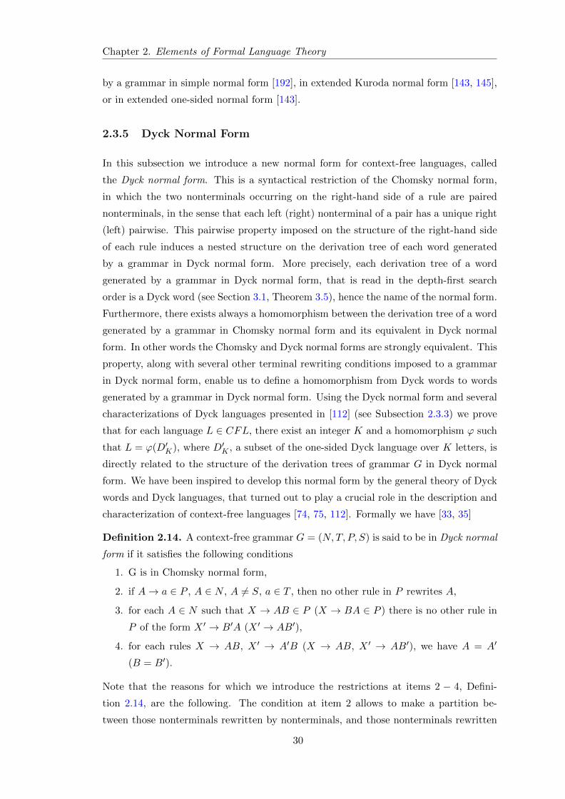
Chapter 2. Elements of Formal Language Theory
by a grammar in simple normal form [192], in extended Kuroda normal form [143, 145],
or in extended one-sided normal form [143].
2.3.5 Dyck Normal Form
In this subsection we introduce a new normal form for context-free languages, called
the Dyck normal form. This is a syntactical restriction of the Chomsky normal form,
in which the two nonterminals occurring on the right-hand side of a rule are paired
nonterminals, in the sense that each left (right) nonterminal of a pair has a unique right
(left) pairwise. This pairwise property imposed on the structure of the right-hand side
of each rule induces a nested structure on the derivation tree of each word generated
by a grammar in Dyck normal form. More precisely, each derivation tree of a word
generated by a grammar in Dyck normal form, that is read in the depth-first search
order is a Dyck word (see Section 3.1, Theorem 3.5), hence the name of the normal form.
Furthermore, there exists always a homomorphism between the derivation tree of a word
generated by a grammar in Chomsky normal form and its equivalent in Dyck normal
form. In other words the Chomsky and Dyck normal forms are strongly equivalent. This
property, along with several other terminal rewriting conditions imposed to a grammar
in Dyck normal form, enable us to define a homomorphism from Dyck words to words
generated by a grammar in Dyck normal form. Using the Dyck normal form and several
characterizations of Dyck languages presented in [112] (see Subsection 2.3.3) we prove
that for each language L ∈ CFL, there exist an integer K and a homomorphism ϕ such
that L = ϕ(D′K), where D′K , a subset of the one-sided Dyck language over K letters, is
directly related to the structure of the derivation trees of grammar G in Dyck normal
form. We have been inspired to develop this normal form by the general theory of Dyck
words and Dyck languages, that turned out to play a crucial role in the description and
characterization of context-free languages [74, 75, 112]. Formally we have [33, 35]
Definition 2.14. A context-free grammar G = (N,T, P, S) is said to be in Dyck normal
form if it satisfies the following conditions
1. G is in Chomsky normal form,
2. if A→ a ∈ P , A ∈ N , A 6= S, a ∈ T , then no other rule in P rewrites A,
3. for each A ∈ N such that X → AB ∈ P (X → BA ∈ P ) there is no other rule in
P of the form X ′ → B′A (X ′ → AB′),
4. for each rules X → AB, X ′ → A′B (X → AB, X ′ → AB′), we have A = A′
(B = B′).
Note that the reasons for which we introduce the restrictions at items 2 − 4, Defini-
tion 2.14, are the following. The condition at item 2 allows to make a partition be-
tween those nonterminals rewritten by nonterminals, and those nonterminals rewritten
30
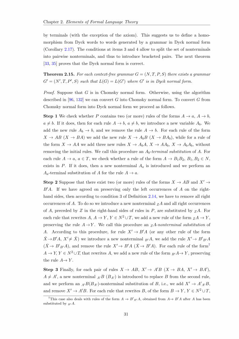
Chapter 2. Elements of Formal Language Theory
by terminals (with the exception of the axiom). This suggests us to define a homo-
morphism from Dyck words to words generated by a grammar in Dyck normal form
(Corollary 2.17). The conditions at items 3 and 4 allow to split the set of nonterminals
into pairwise nonterminals, and thus to introduce bracketed pairs. The next theorem
[33, 35] proves that the Dyck normal form is correct.
Theorem 2.15. For each context-free grammar G = (N,T, P, S) there exists a grammar
G′ = (N ′, T, P ′, S) such that L(G) = L(G′) where G′ is in Dyck normal form.
Proof. Suppose that G is in Chomsky normal form. Otherwise, using the algorithm
described in [96, 132] we can convert G into Chomsky normal form. To convert G from
Chomsky normal form into Dyck normal form we proceed as follows.
Step 1 We check whether P contains two (or more) rules of the forms A → a, A → b,
a 6= b. If it does, then for each rule A → b, a 6= b, we introduce a new variable Ab. We
add the new rule Ab → b, and we remove the rule A → b. For each rule of the form
X → AB (X → BA) we add the new rule X → AbB (X → BAb), while for a rule of
the form X → AA we add three new rules X → AbA, X → AAb, X → AbAb, without
removing the initial rules. We call this procedure an Ab-terminal substitution of A. For
each rule A → a, a ∈ T , we check whether a rule of the form A → B1B2, B1, B2 ∈ N ,
exists in P . If it does, then a new nonterminal Aa is introduced and we perform an
Aa-terminal substitution of A for the rule A→ a.
Step 2 Suppose that there exist two (or more) rules of the forms X → AB and X ′ →B′A. If we have agreed on preserving only the left occurrences of A on the right-
hand sides, then according to condition 3 of Definition 2.14, we have to remove all right
occurrences of A. To do so we introduce a new nonterminal ZA and all right occurrences
of A, preceded by Z in the right-hand sides of rules in P , are substituted by ZA. For
each rule that rewrites A, A→ Y , Y ∈ N2 ∪T , we add a new rule of the form ZA→ Y ,
preserving the rule A→Y . We call this procedure an ZA-nonterminal substitution of
A. According to this procedure, for rule X ′ → B′A (or any other rule of the form
X→B′A, X ′ 6= X) we introduce a new nonterminal B′A, we add the rule X ′→ B′B′A
(X→ B′B′A), and remove the rule X ′→ B′A (X→ B′A). For each rule of the form7
A→ Y, Y ∈ N2∪T, that rewrites A, we add a new rule of the form B′A→ Y , preserving
the rule A→ Y .
Step 3 Finally, for each pair of rules X→ AB, X ′→ A′B (X→ BA, X ′→ BA′),
A 6= A′, a new nonterminal A′B (BA′) is introduced to replace B from the second rule,
and we perform an A′B(BA′)-nonterminal substitution of B, i.e., we add X ′ → A′A′B,
and remove X ′ → A′B. For each rule that rewrites B, of the form B → Y , Y ∈ N2 ∪T ,
7This case also deals with rules of the form A → B′B′A, obtained from A→ B′A after A has beensubstituted by B′A.
31
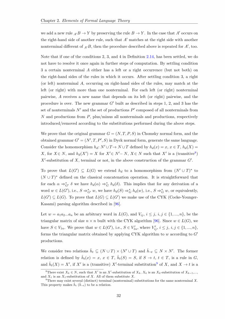
Chapter 2. Elements of Formal Language Theory
we add a new rule A′B → Y by preserving the rule B → Y . In the case that A′ occurs on
the right-hand side of another rule, such that A′ matches at the right side with another
nonterminal different of A′B, then the procedure described above is repeated for A′, too.
Note that if one of the conditions 2, 3, and 4 in Definition 2.14, has been settled, we do
not have to resolve it once again in further steps of computation. By settling condition
3 a certain nonterminal A either has a left or a right occurrence (but not both) on
the right-hand sides of the rules in which it occurs. After settling condition 3, a right
(or left) nonterminal A, occurring on right-hand sides of the rules, may match at the
left (or right) with more than one nonterminal. For each left (or right) nonterminal
pairwise, A receives a new name that depends on its left (or right) pairwise, and the
procedure is over. The new grammar G′ built as described in steps 1, 2, and 3 has the
set of nonterminals N ′ and the set of productions P ′ composed of all nonterminals from
N and productions from P , plus/minus all nonterminals and productions, respectively
introduced/removed according to the substitutions performed during the above steps.
We prove that the original grammar G = (N,T, P, S) in Chomsky normal form, and the
obtained grammar G′ = (N ′, T, P ′, S) in Dyck normal form, generate the same language.
Consider the homomorphism hd: N′ ∪T→ N ∪T defined by hd(x) = x, x ∈ T , hd(X) =
X, for X∈ N , and hd(X′) = X for X ′∈ N ′−N , X∈ N such that X ′ is a (transitive8)
X ′-substitution of X, terminal or not, in the above construction of the grammar G′.
To prove that L(G′) ⊆ L(G) we extend hd to a homomorphism from (N ′ ∪ T )∗ to
(N ∪ T )∗ defined on the classical concatenation operation. It is straightforward that
for each α ⇒∗G′ δ we have hd(α) ⇒∗G hd(δ). This implies that for any derivation of a
word w ∈ L(G′), i.e., S ⇒∗G′ w, we have hd(S)⇒∗G hd(w), i.e., S ⇒∗G w, or equivalently,
L(G′) ⊆ L(G). To prove that L(G) ⊆ L(G′) we make use of the CYK (Cocke-Younger-
Kasami) parsing algorithm described in [96].
Let w = a1a2...an be an arbitrary word in L(G), and Vij , i ≤ j, i, j ∈ 1, ..., n, be the
triangular matrix of size n× n built with the CYK algorithm [96]. Since w ∈ L(G), we
have S ∈ V1n. We prove that w ∈ L(G′), i.e., S ∈ V ′1n, where V ′ij , i ≤ j, i, j ∈ 1, ..., n,forms the triangular matrix obtained by applying CYK algorithm to w according to G′
productions.
We consider two relations ht ⊆ (N ∪ T ) × (N ′ ∪ T ) and h¬t ⊆ N × N ′. The former
relation is defined by ht(x) = x, x ∈ T , ht(S) = S, if S → t, t ∈ T , is a rule in G,
and ht(X) = X ′, if X ′ is a (transitive) X ′-terminal substitution9 of X, and X → t is a
8There exist Xk ∈ N , such that X ′ is an X ′-substitution of Xk, Xk is an Xk-substitution of Xk−1,...,and X1 is an X1-substitution of X. All of them substitute X.
9There may exist several (distinct) terminal (nonterminal) substitutions for the same nonterminal X.This property makes ht (h¬t) to be a relation.
32
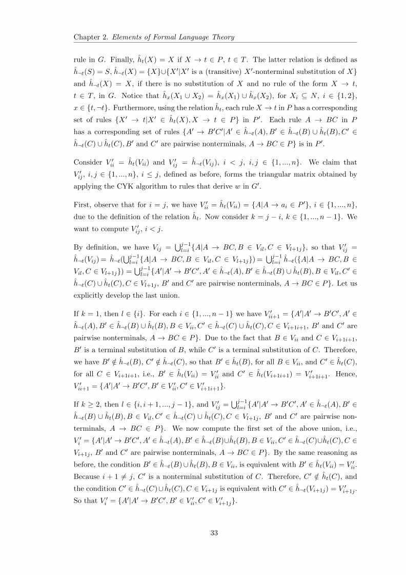
Chapter 2. Elements of Formal Language Theory
rule in G. Finally, ht(X) = X if X → t ∈ P , t ∈ T . The latter relation is defined as
h¬t(S) = S, h¬t(X) = X∪X ′|X ′ is a (transitive) X ′-nonterminal substitution of Xand h¬t(X) = X, if there is no substitution of X and no rule of the form X → t,
t ∈ T , in G. Notice that hx(X1 ∪ X2) = hx(X1) ∪ hx(X2), for Xi ⊆ N , i ∈ 1, 2,x ∈ t,¬t. Furthermore, using the relation ht, each ruleX → t in P has a corresponding
set of rules X ′ → t|X ′ ∈ ht(X), X → t ∈ P in P ′. Each rule A → BC in P
has a corresponding set of rules A′ → B′C ′|A′ ∈ h¬t(A), B′ ∈ h¬t(B) ∪ ht(B), C ′ ∈h¬t(C) ∪ ht(C), B′ and C ′ are pairwise nonterminals, A→ BC ∈ P is in P ′.
Consider V ′ii = ht(Vii) and V ′ij = h¬t(Vij), i < j, i, j ∈ 1, ..., n. We claim that
V ′ij , i, j ∈ 1, ..., n, i ≤ j, defined as before, forms the triangular matrix obtained by
applying the CYK algorithm to rules that derive w in G′.
First, observe that for i = j, we have V ′ii = ht(Vii) = A|A → ai ∈ P ′, i ∈ 1, ..., n,due to the definition of the relation ht. Now consider k = j − i, k ∈ 1, ..., n − 1. We
want to compute V ′ij , i < j.
By definition, we have Vij =⋃j−1l=i A|A → BC,B ∈ Vil, C ∈ Vl+1j, so that V ′ij =
h¬t(Vij) = h¬t(⋃j−1l=i A|A → BC,B ∈ Vil, C ∈ Vl+1j) =
⋃j−1l=i h¬t(A|A → BC,B ∈
Vil, C ∈ Vl+1j) =⋃j−1l=i A
′|A′ → B′C ′, A′ ∈ h¬t(A), B′ ∈ h¬t(B) ∪ ht(B), B ∈ Vil, C ′ ∈h¬t(C) ∪ ht(C), C ∈ Vl+1j , B
′ and C ′ are pairwise nonterminals, A→ BC ∈ P. Let us
explicitly develop the last union.
If k = 1, then l ∈ i. For each i ∈ 1, ..., n − 1 we have V ′ii+1 = A′|A′ → B′C ′, A′ ∈h¬t(A), B′ ∈ h¬t(B) ∪ ht(B), B ∈ Vii, C ′ ∈ h¬t(C) ∪ ht(C), C ∈ Vi+1i+1, B′ and C ′ are
pairwise nonterminals, A → BC ∈ P. Due to the fact that B ∈ Vii and C ∈ Vi+1i+1,
B′ is a terminal substitution of B, while C ′ is a terminal substitution of C. Therefore,
we have B′ /∈ h¬t(B), C ′ /∈ h¬t(C), so that B′ ∈ ht(B), for all B ∈ Vii, and C ′ ∈ ht(C),
for all C ∈ Vi+1i+1, i.e., B′ ∈ ht(Vii) = V ′ii and C ′ ∈ ht(Vi+1i+1) = V ′i+1i+1. Hence,
V ′ii+1 = A′|A′ → B′C ′, B′ ∈ V ′ii, C ′ ∈ V ′i+1i+1.
If k ≥ 2, then l ∈ i, i + 1, ..., j − 1, and V ′ij =⋃j−1l=i A
′|A′ → B′C ′, A′ ∈ h¬t(A), B′ ∈h¬t(B) ∪ ht(B), B ∈ Vil, C ′ ∈ h¬t(C) ∪ ht(C), C ∈ Vl+1j , B
′ and C ′ are pairwise non-
terminals, A → BC ∈ P. We now compute the first set of the above union, i.e.,
V ′i = A′|A′ → B′C ′, A′ ∈ h¬t(A), B′ ∈ h¬t(B)∪ht(B), B ∈ Vii, C ′ ∈ h¬t(C)∪ht(C), C ∈Vi+1j , B
′ and C ′ are pairwise nonterminals, A → BC ∈ P. By the same reasoning as
before, the condition B′ ∈ h¬t(B)∪ ht(B), B ∈ Vii, is equivalent with B′ ∈ ht(Vii) = V ′ii.
Because i + 1 6= j, C ′ is a nonterminal substitution of C. Therefore, C ′ /∈ ht(C), and
the condition C ′ ∈ h¬t(C)∪ ht(C), C ∈ Vi+1j is equivalent with C ′ ∈ h¬t(Vi+1j) = V ′i+1j .
So that V ′i = A′|A′ → B′C ′, B′ ∈ V ′ii, C ′ ∈ V ′i+1j.
33
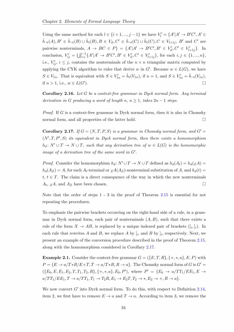
Chapter 2. Elements of Formal Language Theory
Using the same method for each l ∈ i+ 1, ..., j − 1 we have V ′l = A′|A′ → B′C ′, A′ ∈h¬t(A), B′ ∈ h¬t(B) ∪ ht(B), B ∈ Vil, C
′ ∈ h¬t(C) ∪ ht(C), C ∈ Vl+1j , B′ and C ′ are
pairwise nonterminals, A → BC ∈ P = A′|A′ → B′C ′, B′ ∈ V ′il, C′ ∈ V ′l+1j. In
conclusion, V ′ij =⋃j−1l=i A
′|A′ → B′C ′, B′ ∈ V ′il, C ′ ∈ V ′l+1j, for each i, j ∈ 1, ..., n,i.e., V ′ij , i ≤ j, contains the nonterminals of the n × n triangular matrix computed by
applying the CYK algorithm to rules that derive w in G′. Because w ∈ L(G), we have
S ∈ V1n. That is equivalent with S ∈ V ′1n = ht(V1n), if n = 1, and S ∈ V ′1n = h¬t(V1n),
if n > 1, i.e., w ∈ L(G′).
Corollary 2.16. Let G be a context-free grammar in Dyck normal form. Any terminal
derivation in G producing a word of length n, n ≥ 1, takes 2n− 1 steps.
Proof. If G is a context-free grammar in Dyck normal form, then it is also in Chomsky
normal form, and all properties of the latter hold.
Corollary 2.17. If G = (N,T, P, S) is a grammar in Chomsky normal form, and G′ =
(N ′, T, P ′, S) its equivalent in Dyck normal form, then there exists a homomorphism
hd : N ′ ∪ T → N ∪ T , such that any derivation tree of w ∈ L(G) is the homomorphic
image of a derivation tree of the same word in G′.
Proof. Consider the homomorphism hd: N′ ∪ T → N ∪ T defined as hd(At) = hd(ZA) =
hd(AZ) = A, for each At-terminal or ZA(AZ)-nonterminal substitution of A, and hd(t) =
t, t ∈ T . The claim is a direct consequence of the way in which the new nonterminals
At, ZA, and AZ have been chosen.
Note that the order of steps 1 - 3 in the proof of Theorem 2.15 is essential for not
repeating the procedures.
To emphasis the pairwise brackets occurring on the right-hand side of a rule, in a gram-
mar in Dyck normal form, each pair of nonterminals (A,B), such that there exists a
rule of the form X → AB, is replaced by a unique indexed pair of brackets ([i, ]i). In
each rule that rewrites A and B, we replace A by [i, and B by ]i, respectively. Next, we
present an example of the conversion procedure described in the proof of Theorem 2.15,
along with the homomorphism considered in Corollary 2.17.
Example 2.1. Consider the context-free grammar G = (E, T,R, +, ∗, a, E, P ) with
P = E → a/T ∗R/E+T, T → a/T ∗R,R→ a. The Chomsky normal form of G is G′ =
(E0, E,E1, E2, T, T1, T2, R, +, ∗, a, E0, P′), where P ′ = E0 → a/TT1/EE1, E →
a/TT1/EE1, T → a/TT1, T1 → T2R,E1 → E2T, T2 → ∗, E2 → +, R→ a.
We now convert G′ into Dyck normal form. To do this, with respect to Definition 2.14,
item 2, we first have to remove E → a and T → a. According to item 3, we remove the
34
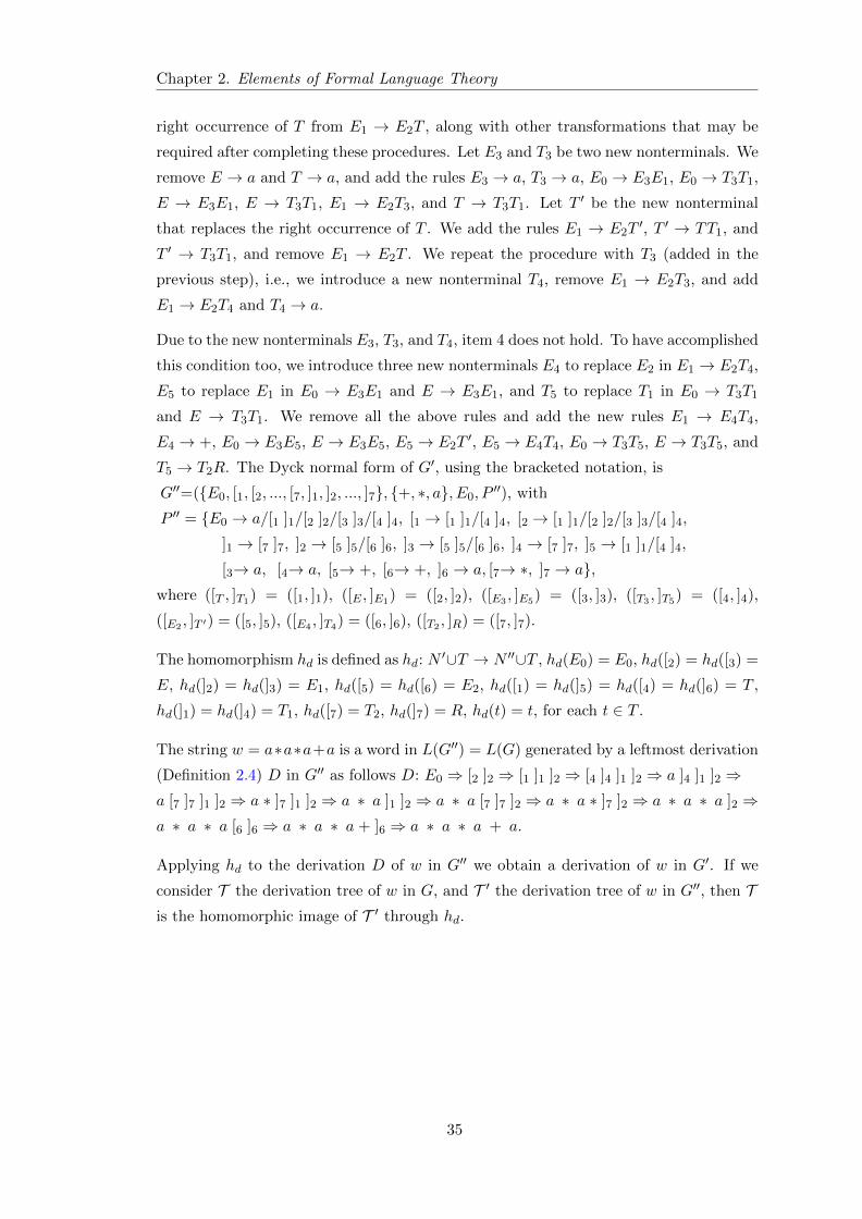
Chapter 2. Elements of Formal Language Theory
right occurrence of T from E1 → E2T , along with other transformations that may be
required after completing these procedures. Let E3 and T3 be two new nonterminals. We
remove E → a and T → a, and add the rules E3 → a, T3 → a, E0 → E3E1, E0 → T3T1,
E → E3E1, E → T3T1, E1 → E2T3, and T → T3T1. Let T ′ be the new nonterminal
that replaces the right occurrence of T . We add the rules E1 → E2T′, T ′ → TT1, and
T ′ → T3T1, and remove E1 → E2T . We repeat the procedure with T3 (added in the
previous step), i.e., we introduce a new nonterminal T4, remove E1 → E2T3, and add
E1 → E2T4 and T4 → a.
Due to the new nonterminals E3, T3, and T4, item 4 does not hold. To have accomplished
this condition too, we introduce three new nonterminals E4 to replace E2 in E1 → E2T4,
E5 to replace E1 in E0 → E3E1 and E → E3E1, and T5 to replace T1 in E0 → T3T1
and E → T3T1. We remove all the above rules and add the new rules E1 → E4T4,
E4 → +, E0 → E3E5, E → E3E5, E5 → E2T′, E5 → E4T4, E0 → T3T5, E → T3T5, and
T5 → T2R. The Dyck normal form of G′, using the bracketed notation, is
G′′=(E0, [1, [2, ..., [7, ]1, ]2, ..., ]7, +, ∗, a, E0, P′′), with
P ′′ = E0 → a/[1 ]1/[2 ]2/[3 ]3/[4 ]4, [1 → [1 ]1/[4 ]4, [2 → [1 ]1/[2 ]2/[3 ]3/[4 ]4,
]1 → [7 ]7, ]2 → [5 ]5/[6 ]6, ]3 → [5 ]5/[6 ]6, ]4 → [7 ]7, ]5 → [1 ]1/[4 ]4,
[3→ a, [4→ a, [5→ +, [6→ +, ]6 → a, [7→ ∗, ]7 → a,where ([T , ]T1) = ([1, ]1), ([E , ]E1) = ([2, ]2), ([E3 , ]E5) = ([3, ]3), ([T3 , ]T5) = ([4, ]4),
([E2 , ]T ′) = ([5, ]5), ([E4 , ]T4) = ([6, ]6), ([T2 , ]R) = ([7, ]7).
The homomorphism hd is defined as hd: N′∪T → N ′′∪T , hd(E0) = E0, hd([2) = hd([3) =
E, hd(]2) = hd(]3) = E1, hd([5) = hd([6) = E2, hd([1) = hd(]5) = hd([4) = hd(]6) = T ,
hd(]1) = hd(]4) = T1, hd([7) = T2, hd(]7) = R, hd(t) = t, for each t ∈ T .
The string w = a∗a∗a+a is a word in L(G′′) = L(G) generated by a leftmost derivation
(Definition 2.4) D in G′′ as follows D: E0 ⇒ [2 ]2 ⇒ [1 ]1 ]2 ⇒ [4 ]4 ]1 ]2 ⇒ a ]4 ]1 ]2 ⇒a [7 ]7 ]1 ]2 ⇒ a ∗ ]7 ]1 ]2 ⇒ a ∗ a ]1 ]2 ⇒ a ∗ a [7 ]7 ]2 ⇒ a ∗ a ∗ ]7 ]2 ⇒ a ∗ a ∗ a ]2 ⇒a ∗ a ∗ a [6 ]6 ⇒ a ∗ a ∗ a + ]6 ⇒ a ∗ a ∗ a + a.
Applying hd to the derivation D of w in G′′ we obtain a derivation of w in G′. If we
consider T the derivation tree of w in G, and T ′ the derivation tree of w in G′′, then Tis the homomorphic image of T ′ through hd.
35
Chapter 3
Homomorphic Representations
and Regular Approximations of
Languages
“Would you tell me, please, which way I ought to go from here?”
“That depends a good deal on where you want to get to,” said the Cat.”
“I dont much care where” said Alice.
“Then it doesn’t matter which way you
go,” said the Cat.
“so long as I get SOMEWHERE,”
Alice added as an explanation.
“Oh, you’re sure to do that,” said the
Cat, “if you only walk long enough.”
(Lewis Carroll, Alice’s Adventures in
Wonderland)
This chapter is devoted to the homomorphic representations of context-free languages by
means of Dyck languages. We present an alternative proof of the Chomsky-Schutzenberger
theorem. To reach the Chomsky-Schutzenberger theorem, for each context-free grammar
G in Dyck normal form (Definition 2.14) we define, in Section 3.1, the trace-language
associated with derivations in G (Definition 3.2), which is the set of all derivation trees of
G read in the depth-first search order, starting from the grammar axiom. By exploiting
the Dyck normal form, and several characterizations of Dyck languages presented in [112]
36
Chapter 3. Homomorphic Representations and Regular Approximations of Languages
(see also Subsection 2.3.3) we prove that for each context-free language L, generated by
a grammar G in Dyck normal form, there exist an integer K and a homomorphism ϕ
such that L = ϕ(D′K), where D′K (a subset of the Dyck language over K letters) equals
the trace-language associated with G (Theorem 3.6).
In Section 3.2 we show that the representation theorem described in Section 3.1 (Theo-
rem 3.6) emerges, through a transition-like diagram for context-free grammars in Dyck
normal form, to the Chomsky-Schutzenberger theorem. By improving this transition
diagram, in Section 3.3 we refine the regular language in the Chomsky-Schutzenberger
theorem. Then in Section 3.4 we show that the refined graphical representation of deriva-
tions in a context-free grammar in Dyck normal form, built in Section 3.3, provides a
framework for a regular grammar that generates a regular superset approximation for
the initial context-free language.
The method used throughout this chapter is graph-constructive, in the sense that it
supplies a graphical interpretation of the Chomsky-Schutzenberger theorem and conse-
quently it shows how to graphically build a regular language (as minimal as possible)
that satisfies this theorem. Even if we reach a well-known theorem, the method used to
approach it is different from the other methods known in the literature.
Recall that the method described in [96] is based on pushdown approaches, while that in
[84] uses some kind of imaginary brackets that simulate the work of a pushdown store,
when deriving a context-free language. The method presented in [12] uses equations on
languages and algebraical approaches to derive several types of Dyck language generators
for context-free languages. In all these works the Dyck language is somehow hidden
behind the derivative structure of the context-free language (supplementary brackets
are needed to derive a Dyck language generator for a context-free language).
The Dyck language provided by the method proposed in this chapter is merely found
through a pairwise-renaming procedure of the nonterminals in the original context-free
grammar. Hence, it lies inside the context-free grammar it describes. Each method used
in the literature to prove the Chomsky-Schutzenberger theorem provides its own regular
language. Our aim is to find a thiner regular language (see Section 3.3) that satisfies
this theorem (with respect to the method hereby used) and approaching this language to
build a regular superset approximation for context-free languages (likely to be as thiner
as possible).
Note that, the concept of a thiner (minimal) regular language, for the Chomsky-Schutzen-
berger theorem and for the regular superset approximation, provided in this chapter,
is relative, in the sense that it depends on the structure of the grammar in Dyck nor-
mal form used to generate the original context-free language. In [22, 92, 93, 94] it is
37
Chapter 3. Homomorphic Representations and Regular Approximations of Languages
proved that there is no algorithm that builds, for an arbitrary context-free language L,
the minimal context-free grammar that generates L, where the minimality of a context-
free grammar is considered, in principal, with respect to descriptional measures such
as number of nonterminals, rules, and loops (i.e., grammatical levels [92], encountered
during derivations in a context-free grammar). Consequently, there is no algorithm to
build a minimal regular superset approximation for an arbitrary context-free language.
Attempts to find optimal regular superset (subset) approximations for context-free lan-
guages can be found in [43, 71, 155, 194].
In Sections 3.2, 3.3, and 3.4 we also illustrate, through several examples, the manner
in which the regular languages provided by the Chomsky-Schutzenberger theorem and
by the regular approximation can be built, with regards to the method proposed in this
chapter. Results in this chapter are collected from [35].
3.1 Homomorphic Representations of Languages
There are situations in which the elements of a certain class C of languages can be
described in terms of elements of another class C′, upon which there have been ap-
plied some (simple) operations on languages, such as intersection (with another class
C′′), concatenation, or homomorphism. This is what is called the representation (or
characterization) of the class C by means of languages in the class C′. In a good rep-
resentation the class1 C′ is as simple as possible, but in the same time it is rich in
decidability and closure properties, and/or endowed with efficient parsing algorithms.
In this way properties of the class C′ can be inferred by C, assuming that the former class
is closed under the operations applied to it. This is the main reason why characteriza-
tion theorems are extensively used in formal languages, computational and complexity
theory. These facilitate further refinements on computational and complexity results
of languages in C. Due to their computational simplicity, class C′ is usually a regular
language, or a little bit more complicated subclasses of context-free languages, such as
linear context-free or Dyck languages. One of the most famous representation theo-
rem is the Chomsky-Schutzenberger theorem which is a homomorphic representation of
context-free languages, by means of Dyck languages intersected with regular languages.
Theorem 3.1. (Chomsky-Schutzenberger) For each context-free language L there exist
an integer k, a regular set R, and a homomorphism h, such that L = h(Dk ∩R).
Furthermore, the homomorphism h in Theorem 3.1 is non-erasing, assuming that L does
not contain any word of length 1 [162].
1Languages in C′ are also called generators of C.
38
Chapter 3. Homomorphic Representations and Regular Approximations of Languages
Chomsky-Schutzenberger-like theorems, by means of Dyck languages, have been set-
tled for various classes and subclasses of languages in the Chomsky hierarchy, such as
slender context-free languages [64], indexed languages [164], recursively enumerable lan-
guages [100, 101], and Petri nets languages [95]. For instance, according to [100, 101],
any recursively enumerable language is the homomorphic image of the intersection of
a Dyck language with a minimal linear context-free language. These representation
results show that most of the languages in the Chomsky hierarchy can be reduced,
through a homomorphic image, to a Dyck language, modified in a proper way that de-
pends on the grammar formalism we want to characterize. This is advantageous because
Dyck languages are built on symmetrical patterns based on balanced (nested) strings of
parentheses, endowed with many combinatorial and descriptional properties that allow
efficient parsing algorithms. In conclusion, Dyck languages modified in a proper way
may be generators of a large variety of languages.
Next we give an alternative proof of the Chomsky-Schutzenberger theorem based on
graphical approaches. The regular language in this theorem is obtained from a transition-
like diagram associated with derivations in a context-free grammar set in Dyck normal
form (Definition 2.14). In this respect, we introduce some new notions based on the
Dyck normal form of a context-free grammar [33, 35].
Definition 3.2. Let Gk = (Nk, T, Pk, S) be a context-free grammar in Dyck normal
form with |Nk − S| = 2k. Let D : S ⇒ u1 ⇒ u2 ⇒ ...⇒ u2n−1 = w, n ≥ 2, be
a leftmost derivation of w ∈ L(G). The trace-word of w associated with D, denoted
as tw,D, is defined as the concatenation of nonterminals consecutively rewritten in D,
excluding the axiom. The trace-language associated with Gk, denoted as L(Gk), is
L(Gk) = tw,D| for any w ∈ L(Gk), and any leftmost derivation D of w.
Note that tw,D, w ∈ L(G), can also be read from the derivation tree in the depth-
first search order (Section 2.1) starting with the root, but omitting the root and the
leaves. The trace-word associated with w and the leftmost derivation D in Example 2.1
is ta∗a∗a+a,D = [2 [1 [4 ]4 [7 ]7 ]1 [7 ]7 ]2 [6 ]6.
Let Gk = (Nk, T, Pk, S) be a context-free grammar in Dyck normal form. In order
to emphasize possible relations between the structure of the trace-words in L(Gk) and
the structure of words belonging to a Dyck language (Definition 2.9), and also to keep
control of each bracketed pair occurring on the right-hand sides of rules in Gk, we
fix Nk = S, [1, [2, ..., [k, ]1, ]2, ..., ]k, and Pk to be composed of rules of the forms
X → [i ]i, 1 ≤ i ≤ k, and Y → t, X,Y ∈ Nk, t ∈ T .
In the sequel, for a string w, by wi:j we denote the substring of w starting at the ith
position and ending at the jth position. In the next definitions and results we use the
39
Chapter 3. Homomorphic Representations and Regular Approximations of Languages
notion of a matched pair, introduced in Subsection 2.3.3, Definition 2.10. The proof of
Theorem 3.5 is based on Lemmas 2.11 and 2.12 (Subsection 2.3.3).
Definition 3.3. A pair (i, j) is a nested pair of w ∈ Dk, if (i, j) is a matched pair, and
either j = i+ 1, or (i+ 1, j − 1) is a matched pair.
Definition 3.4. Let w ∈ Dk, and (i, j) be a matched pair of w. We say that (i, j)
is reducible if there exists an integer j′, i < j′ < j, such that (i, j′) and (j′ + 1, j) are
matched pairs of w.
If (i, j) is a nested pair of w ∈ Dk then (i, j) is an irreducible pair. If (i, j) is a nested
pair of w then (i+ 1, j − 1) may be a reducible pair.
Theorem 3.5. The trace-language associated with a context-free grammar G = (Nk, T, Pk,
S) in Dyck normal form, with |Nk| = 2k + 1, is a subset of Dk.
Proof. Let Nk = S, [1, ..., [k, ]1, ..., ]k be the set of nonterminals, w ∈ L(G), and
D a leftmost derivation of w. We show, by using Lemma 2.12, that any subtree of
the derivation tree, read in the depth-first search order, by ignoring the root and the
terminal nodes, corresponds to a matched pair in tw,D. In particular, (1, |tw,D|) will be
a matched pair. Denote by tw,Di:j the substring of tw,D starting at the ith position and
ending at the jth position in tw,D. We show that for all matched pairs (i, j), hk′(tw,Di:j)
belong to D1, 1 ≤ k′ ≤ k. We prove these claims by induction on the height of subtrees.
Basis. Any subtree of height n = 1, read in the depth-first search order, is of the form
[i ]i, 1 ≤ i ≤ k. Therefore, it satisfies the above conditions.
Induction step. Assume that the claim is true for all subtrees of height ~, ~ < n, and we
prove it for ~ = n. Each subtree of height n can have one of the following struc-
tures. The level 0 of the subtree is marked by a left or right bracket. This bracket
will not be considered when we read the subtree. Denote by [m the left child of the
root. Then the right child is labeled by ]m. These are the roots of a left and right
subtree, for which at least one has the height n − 1. Suppose that both subtrees have
the height 1 ≤ ~ ≤ n− 1. By the induction hypothesis, let us further suppose that
the left subtree corresponds to the matched pair (il, jl), and the right subtree corre-
sponds to the matched pair (ir, jr), ir = jl+ 2, because the position jl+ 1 is taken
by ]m. As h is a homomorphism, we have h(tw,Dil−1:jr)= h([mtw,Dil:jl ]mtw,Djl+2:jr
)=
h([m)h(tw,Dil:jl)h(]m)h(tw,Djl+2:jr). Hence h(tw,Dil−1:jr
) satisfies all conditions in Defi-
nition 2.10, and thus (il − 1, jr) that corresponds to the considered subtree of height n,
is a matched pair. By the induction hypothesis, hk′(tw,Dil:jl) and hk′(tw,Dir:jr) are in
D1, 1≤ k′≤ k. Therefore, hk′(tw,Dil−1:jr)= hk′([m)hk′(tw,Dil:jl)hk
′(]m)hk′(tw,Djl+2:jr)∈
hk′(tw,Dil:jl)hk′(tw,Djl+2:jr), [1hk′(tw,Dil:jl)]1hk
′(tw,Djl+2:jr), i.e., hk′(tw,Dil−1:jr
)∈ D1.
40
Chapter 3. Homomorphic Representations and Regular Approximations of Languages
Note that in this case the matched pair (il − 1, jr) is reducible into (il − 1, jl + 1) and
(jl+2, jr), where (il−1, jl+1) corresponds to the substring tw,Dil−1:jl+1 = [mtw,Dil:jl ]m.
We refer to this structure as the left embedded subtree, i.e., (il − 1, jl + 1) is a nested
pair. A similar reasoning is applied for the case when one of the subtrees has height
0. Analogously, it can be shown that the initial tree corresponds to the matched pair
(1, |tw,D|), i.e., the first condition of Lemma 2.12 holds.
So far, we have proved that each subtree of the derivation tree and each left embedded
subtree correspond to a matched pair (i, j) and (il, jl), respectively, such that hk′(tw,Di:j)
and hk′([mtw,Dil:jl ]m), 1 ≤ k′ ≤ k, are in D1. Next we show that all matched pairs from
tw,D correspond only to subtrees, or left embedded subtrees, from the derivation tree.
To derive a contradiction, let us suppose that there exists a matched pair (i, j) in tw,D,
that does not correspond to any subtree, or left embedded subtree of the derivation tree
read in the depth-first search order. We show that this leads to a contradiction.
Since (i, j) does not correspond to any subtree, or left embedded subtree, there exist
two adjacent subtrees θ1 (a left embedded subtree) and θ2 (a right subtree) such that
(i, j) is composed of two adjacent “subparts” of θ1 and θ2. In terms of matched pairs,
if θ1 corresponds to the matched pair (i1, j1) and θ2 corresponds to the matched pair
(i2, j2), such that i2 = j1 + 2, then there exist a suffix si1−1:j1+1 of tw,Di1−1:j1+1, and a
prefix pi2:j2 of tw,Di2:j2, such that tw,Di:j= si1−1:j1+1pi2:j2 . Furthermore, without loss of
generality, we assume that (i1, j1) and (i2, j2) are nested pairs. Otherwise, the matched
pair (i, j) can be “narrowed” until θ1 and θ2 are characterized by two nested pairs. If
(i1, j1) is a nested pair, then so is (i1 − 1, j1 + 1).
Since si1−1:j1+1 is a suffix of tw,Di1−1:j1+1 and (i1 − 1, j1 + 1) is a matched pair, with
respect to Definition 2.10, the number of ]1’s in h(si1−1:j1+1) is greater than or equal
to the number of [1’s in h(si1−1:j1+1). On the other hand, si1−1:j1+1 is also a prefix of
tw,Di:j , because (i, j) is a matched pair, by our hypothesis. Therefore, the number of [1’s
in h(si1−1:j1+1) is greater than or equal to the number of ]1’s in h(si1−1:j1+1). Hence, the
only possibility for si1−1:j1+1 to be a suffix for tw,Di1−1:j1+1 and a prefix for tw,Di:j is the
equality between the number of [1’s and ]1’s in h(si1−1:j1+1). This property holds if and
only if si1−1:j1+1 corresponds to a matched pair in tw,Di1−1:j1+1, i.e., if is and js are the
start and the end positions of si1−1:j1+1 in tw,Di1−1:j1+1, then (is, js) is a matched pair.
Thus, (i1−1, j1 + 1) is a reducible pair into (i1−1, is−1) and (is, js), where js = j1 + 1,
and we have reached a contradiction.
Therefore, the matched pairs in tw,D correspond to subtrees, or left embedded subtrees,
in the derivation tree. For these matched pairs we have already proved that they satisfy
the conditions of Lemma 2.12. Accordingly, tw,D ∈ Dk, and consequently the trace-
language associated with G is a subset of Dk.
41
Chapter 3. Homomorphic Representations and Regular Approximations of Languages
Theorem 3.6. Given a context-free grammar G there exist an integer K, a homo-
morphism ϕ, and a subset D′K of the Dyck language DK , such that L(G) = ϕ(D′K).
Furthermore, if G has no rules of the form S → t, where t is a terminal, then D′K equals
the trace-language associated with G in Dyck normal form. Otherwise, D′K is a very
small extension of the trace-language of grammar G in Dyck normal form.
Proof. Let G be a context-free grammar and Gk= (Nk, T, Pk, S) the Dyck normal form
of G, such that Nk = S, [1, [2, ..., [k, ]1, ]2, ..., ]k. Let L(Gk) be the trace-language asso-
ciated with Gk. Consider tk+1, ..., tk+p the ordered subset of T where S → tk+i ∈ P ,
1≤ i≤ p. Define Nk+p = Nk ∪ [tk+1, ..., [tk+p
, ]tk+1, ...]tk+p
, and Pk+p = (Pk − S→tk+i ∈ P |1≤ i ≤ p) ∪ S → [tk+i
]tk+i, [tk+i
→ tk+i, ]tk+i→ λ | S → tk+i ∈ P, 1≤ i ≤ p,
then the grammar Gk+p = (Nk+p, T, Pk+p, S) has the property that L(Gk+p) = L(Gk).
Let ϕ : (Nk+p − S)∗→ T ∗ be the homomorphism defined by ϕ(N) = λ, for each
rule of the form N→ XY , N,X, Y ∈ Nk − S, and ϕ(N) = t, for each rule of the
form N → t, N ∈ Nk − S, and t ∈ T , ϕ([k+i) = tk+i, and ϕ(]k+i) = λ, for each
1≤ i≤ p. It is evident that L= ϕ(D′K), where K= k + p, D′K= L(Gk) ∪ Lp(Gk), and
Lp(Gk) = [tk+1]tk+1
, ..., [tk+p]tk+p. If G has no rule of the form S → t, t ∈ T ∪λ, then
Lp(Gk) = and D′K = L(Gk).
In the sequel, grammar Gk+p is called the extended grammar of Gk. Gk has an extended
grammar if and only if Gk (or G) has rules of the form S → t, t ∈ T ∪λ. Recall that, if
Gk does not have an extended grammar then D′K = D′k = L(Gk). This property makes
the subset D′k+p (D′k) of the Dyck language Dk+p (respectively, Dk) to be characteristic
to context-free languages.
3.2 Further Remarks on the Structure of Context-Free
Languages and Homomorphic Representation
Let Gk = (Nk, T, Pk, S) be an arbitrary context-free grammar in Dyck normal form,
with Nk = S, [1, [2, ..., [k, ]1, ]2, ..., ]k. Let ϕ: (Nk − S)∗ → T ∗ be a restriction of the
homomorphism introduced in the proof of Theorem 3.6, defined as follows ϕ(λ) = λ,
ϕ(N) = λ, for each rule of the form N → XY , N,X, Y ∈ Nk − S, and ϕ(N) = t, for
each rule of the form N → t, N ∈ Nk −S, t ∈ T . Next we divide Nk −S into three
main sets N (1), N (2), N (3) as follows
1. [i, ]i ∈ N (1) if and only if ϕ([i), ϕ(]i) ∈ T ,
2. [i, ]i ∈ N (2) if and only if ϕ([i) ∈ T and ϕ(]i) = λ, or if ϕ([i) = λ and ϕ(]i) ∈ T ,
3. [i, ]i ∈ N (3) if and only ϕ([i) = ϕ(]i) = λ.
42
Chapter 3. Homomorphic Representations and Regular Approximations of Languages
The set N (2) is further divided into N(2)l and N
(2)r , such that N
(2)l contains all bracketed-
pairs [i, ]i ∈ N (2) such that ϕ([i) 6= λ, and N(2)r contains all bracketed-pairs [i, ]i∈ N (2)
such that ϕ(]i) 6= λ. We have N (2)= N(2)l ∪N
(2)r and N
(2)l ∩N
(2)r = ∅, i.e., N (2)
l , N(2)r is
a partition of N (2). Besides, N (1), N (2), N (3) is a partition of Nk − S. Note that if
[i ∈ X (or ]i∈ X), X∈ N (1), N (2), N (3), N(2)l , N
(2)r , then ]i∈ X ([i∈ X). Sometimes, to
emphasize that a bracket [i or ]i produces a terminal symbol, we use for it the notation
[ti or ]ti if [i ∈ N (2)l or ]i ∈ N (2)
r , respectively. We use the notation [ti and ]ti if [i, ]i ∈ N (1).
Definition 3.7. A grammar Gk is in linear-Dyck normal form if Gk is in Dyck normal
form and N (3) = ∅.
Theorem 3.8. For each linear grammar G, there exits a grammar Gk in linear-Dyck
normal form such that L(G) = L(Gk), and vice versa.
Proof. Each linear grammar G can be written in a standard form using only rules of the
forms X→λ, X→ t, X→ t1Y , X→ Y t2, X→ t1Y t2, t, t1, t2 ∈ T , X,Y ∈ N . Trans-
forming G from standard form into the Chomsky normal form, and then into the Dyck
normal form, we obtain a grammar Gk in linear-Dyck normal form. As standard, Chom-
sky, and Dyck normal forms for linear context-free language are weakly equivalent we
have L(G) = L(Gk).
Corollary 3.9. LINL is equal with the family of languages generated by grammars in
linear-Dyck normal form.
In the sequel we consider more closely the structures of the derivation trees (Defini-
tion 2.6) associated with words generated by linear and context-free grammars in linear-
Dyck and Dyck normal forms, respectively. We are interested in the structure of the
trace-words associated with words generated by these grammars.
Let Gk = (Nk, T, Pk, S) be an arbitrary (linear) context-free grammar in (linear-)Dyck
normal form, and L(Gk) the language generated by this grammar. Let w ∈ L(Gk), D a
leftmost derivation of w, and tw,D the trace-word of w associated with D (Definition 3.2).
From the structure of the derivation tree of w, read in the depth-first search order, it is
easy to observe that each bracket [i ∈ N (1) is immediately followed in tw,D by its pairwise
]i. The same property holds for the pairs of brackets [i, ]i ∈ N (2)l . If [i, ]i ∈ N (2)
r ∪N (3)
then the pair [i, ]i should embed a left subtree, i.e., the case of the left embedded subtree
in the proof of Theorem 3.5. In this case the bracket [i may have a long distance
placement from its pairwise ]i, in tw,D.
Suppose that Gk is a linear grammar in linear-Dyck normal form, i.e., N (3) = ∅, such
that both N(2)r and N
(2)l are non-empty. Each word w = a1a2...an, of an arbitrary length
43
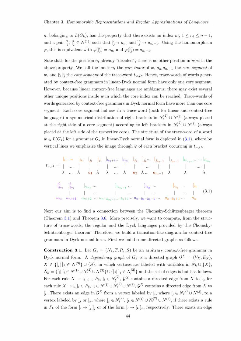
Chapter 3. Homomorphic Representations and Regular Approximations of Languages
n, belonging to L(Gk), has the property that there exists an index nt, 1 ≤ nt ≤ n − 1,
and a pair [tj , ]tj ∈ N (1), such that [tj→ ant and ]tj → ant+1. Using the homomorphism
ϕ, this is equivalent with ϕ([tj) = ant and ϕ(]tj) = ant+1.
Note that, for the position nt already “decided”, there is no other position in w with the
above property. We call the index nt the core index of w, antant+1 the core segment of
w, and [tj ]tj the core segment of the trace-word tw,D. Hence, trace-words of words gener-
ated by context-free grammars in linear-Dyck normal form have only one core segment.
However, because linear context-free languages are ambiguous, there may exist several
other unique positions inside w in which the core index can be reached. Trace-words of
words generated by context-free grammars in Dyck normal form have more than one core
segment. Each core segment induces in a trace-word (both for linear and context-free
languages) a symmetrical distribution of right brackets in N(2)r ∪ N (3) (always placed
at the right side of a core segment) according to left brackets in N(2)r ∪ N (3) (always
placed at the left side of the respective core). The structure of the trace-word of a word
w ∈ L(Gk) for a grammar Gk in linear-Dyck normal form is depicted in (3.1), where by
vertical lines we emphasize the image through ϕ of each bracket occurring in tw,D.
tw,D =
[i1 ... [ik1[j1 ]j1 [ik1+1... [ik2
[j2 ]j2 ... [jnt−1]jnt−1
[iknt−1+1... [iknt
| ... | | | | ... | | | ... | | | ... |λ ... λ a1 λ λ ... λ a2 λ ... ant−1 λ λ λ
[tjnt]tjnt
]iknt... ]iknt−1
... ]ik2... ]ik1
... ]i1
| | | ... | ... | ... | ... |ant ant+1 ant+2 ... an−knt−1...−k1+1 ...an−k2−k1+1 ... an−k1+1 ... an
(3.1)
Next our aim is to find a connection between the Chomsky-Schutzenberger theorem
(Theorem 3.1) and Theorem 3.6. More precisely, we want to compute, from the struc-
ture of trace-words, the regular and the Dyck languages provided by the Chomsky-
Schutzenberger theorem. Therefore, we build a transition-like diagram for context-free
grammars in Dyck normal form. First we build some directed graphs as follows.
Construction 3.1. Let Gk = (Nk, T, Pk, S) be an arbitrary context-free grammar in
Dyck normal form. A dependency graph of Gk is a directed graph GX = (VX , EX),
X ∈ ]j | ]j ∈ N (3) ∪ S, in which vertices are labeled with variables in Nk ∪ X,Nk = [i| [i ∈ N (1)∪N (2)
r ∪N (3)∪]j | ]j ∈ N (2)l and the set of edges is built as follows.
For each rule X → [i ]i ∈ Pk, ]i ∈ N (2)l , GX contains a directed edge from X to ]i, for
each rule X → [i ]i ∈ Pk, [i ∈ N (1) ∪N (2)r ∪N (3), GX contains a directed edge from X to
[i. There exists an edge in GX from a vertex labeled by [i, where [i ∈ N (2)r ∪N (3), to a
vertex labeled by ]j or [k, where ]j ∈ N (2)l , [k ∈ N (1) ∪N (2)
r ∪N (3), if there exists a rule
in Pk of the form [i → [j ]j or of the form [i → [k ]k, respectively. There exists an edge
44
Chapter 3. Homomorphic Representations and Regular Approximations of Languages
in GX from a vertex labeled by ]i, where ]i ∈ N (2)l , to a vertex labeled by ]j or by [k,
where ]j ∈ N (2)l , [k ∈ N (1) ∪N (2)
r ∪N (3), if there exists a rule in Pk of the form ]i → [j ]j
or of the form ]i → [k ]k, respectively. The vertex labeled by X is the initial vertex of
GX . Any vertex labeled by a left bracket in N (1) is a final vertex.
We recall (see Section 2.1) that a cycle or loop in a graph is a simple path from v to v.
If from v to v there is no other vertex then the loop is called self-loop. The cycle rank of
a graph is a measure of the loop complexity formally defined and studied in [29, 72, 91].
It is trivial to prove, by induction on the number of vertices, that the cycle rank of a
digraph, with a finite number of vertices, is finite. In brief, the rank of a cycle C is 1 if
there exists v ∈ C such that C − v is not a cycle. Recursively, the rank of a cycle C is k if
there exists v ∈ C such that C − v contain a cycle of rank k − 1 and all the other cycles
in C − v have the rank at most k − 1.
In [72] it is proved that from each two vertices u and v belonging to a digraph of cycle
rank k, there exists a regular expression of star-height2 at most k that describes the set
of paths from u to v. On the other hand, the cycle rank of a digraph with n vertices is
upper bounded by n log n [91]. Hence, any regular expression obtained from a digraph
with n vertices has the star-height at most n log n.
Let GX be a dependency graph of Gk. Consider the set of all possible paths in GX
starting from the initial vertex to a final vertex. Such a path is called terminal path.
According to the above observations, the (infinite) set of paths from an initial vertex to
a final vertex in GX , can be divided into a finite number of classes of terminal paths.
Paths belonging to the same class are characterized by the same regular expression, in
terms of ∗ and +-Kleene operations, of star-height at most |VX | log |VX | (which is finite
related to the lengths of strings in L(Gk)).
Denote by RX[ti
the set of all regular expressions over Nk ∪ X that can be read in GX ,
starting from the initial vertex X and ending in the final vertex [ti. The cardinality ofRX[ti
is finite. Define the homomorphism hG : Nk∪X → ]i| ]i ∈ N(2)r ∪N (3)∪λ such that
hG([i) = ]i for any [i ∈ N (2)r ∪N (3), hG(X) = hG([ti) = hG(]i) = λ, for any [ti ∈ N (1) and
[i ∈ N (2)l . For any element r.e
(l,X)
[ti∈ RX
[tiwe build a new regular expression3 r.e
(r,X)
[ti=
hrG(r.e(l,X)
[ti), where hrG is the mirror image of hG . Consider r.eX
[ti= r.e
(l,X)
[tir.e
(r,X)
[ti. For
a certain X and [ti, denote by R.eX[ti
the set of all regular expressions r.eX[ti
obtained as
above. Furthermore, R.eX =⋃
[ti∈N(1) R.eX[ti and R.e = R.eS ∪ (⋃
]i∈N(3) R.e]i).
2Informally, this is the (maximal) power of a nested star-loop occurring in the description of a regularexpression. For the formal definition the reader is referred to [72, 98] (see also Definition 3.11).
3Since regular languages are closed under homomorphism and the reverse operation, r.e(r,X)
[tiis a
regular expression.
45
Chapter 3. Homomorphic Representations and Regular Approximations of Languages
Construction 3.2. Let Gk = (Nk, T, Pk, S) be a context-free grammar in Dyck normal
form and GX | X∈ ]j | ]j∈ N (3)∪S the set of dependency graphs of Gk. The exten-
ded dependency graph of Gk, denoted as Ge = (Ve, Ee), is a directed graph for which Ve =
Nk ∪ S ∪ ]i| ]i∈ N(2)r ∪N (3), S is the initial vertex of Ge and Ee is built as follows4:
1. - S[i (or S]j) - there exists an edge in Ge from the vertex labeled by S to a vertex
labeled by [i (from S to ]j), [i ∈ N (1) ∪N (2)r ∪N (3) (]j ∈ N (2)
l ), if there exists a regular
expression in R.eS with a prefix of the form S[i (S]j , respectively).
2. - ]i]j - there exists an edge in Ge from a vertex labeled by ]i to a vertex labeled by ]j
]i, ]j ∈ N (2)l , if there exists a regular expression in R.e having a substring of the form
]i]j (if i = j then ]i]i forms a self-loop in Ge).
3. - ]i[j (or [j ]i) - there exists an edge in Ge from a vertex labeled by ]i to a vertex labeled
by [j (or vice versa from [j to ]i) such that ]i ∈ N (2)l and [j ∈ N (2)
r ∪N (3), if there exists
a regular expression in R.e having a substring of the form ]i[j ([j ]i, respectively).
4. - [i[j - there exists an edge in Ge from a vertex labeled by [i to a vertex labeled by [j ,
[i, [j ∈ N (2)r ∪N (3), if there exists a regular expression in R.e having a substring of the
form [i[j (if i = j then [i[i forms a self-loop in Ge).
5. - ]i[tj (or [i[
tj) - there exists an edge in Ge from a vertex labeled by ]i (or by [i) to a
vertex labeled by [tj , where ]i ∈ N (2)l (or [i ∈ N (2)
r , respectively) and [tj ∈ N (1), if there
exists a regular expression in R.e with a substring of the form ]i[tj ([i[
tj , respectively).
6. - ]j [ti - there exists an edge in Ge from a vertex labeled by ]j to a vertex labeled by [ti,
]j ∈ N (3), [ti ∈ N (1), if there exists a regular expression in R.e]j[ti
of the form ]j [ti.
7. - ]j [i (or ]j ]i) - there exists an edge in Ge from a vertex labeled by ]j to a vertex
labeled by [i, where ]j ∈ N (3), [i ∈ N (2)r (]i ∈ N (2)
l , respectively), if there exists a regular
expression in R.e]j with a prefix of the form ]j [i (]j ]i, respectively).
8. - ]i]j (or [ti]j) - there exists an edge in Ge from a vertex ]i (respectively, from [ti) to
a vertex labeled by ]j , where ]i ∈ N(2)r ([ti ∈ N (1)) and ]j ∈ N
(2)r ∪ N (3) (i and j not
necessarily distinct if ]i, ]j ∈ N (2)r ), if either i., ii., or iii. holds:
i. there exists at least one regular expression in R.e having a substring of the form
]i]j ([ti]j , respectively) (if i = j then ]i]i is a self-loop in Ge),ii. there exists ]k ∈ N (3) and a regular expression in R.e having a substring of the
form ]k]j , and a regular expression in R.e]k that ends in ]i ([ti, respectively) (if i = j then
]i]i is a self-loop).
iii. there exist ]k, ]k1 , ..., ]km ∈ N (3) and a regular expression in R.e having a substring
of the form ]k]j , a regular expression in R.e]k that ends in ]k1 , a regular expression in
4At the beginning of each item we pose the type of the edge defined by that item.
46
Chapter 3. Homomorphic Representations and Regular Approximations of Languages
R.e]k1 that ends in ]k2 , and so on, until a regular expression in R.e]km−1 ending in ]km
and a regular expression in R.e]km ending in ]i ([ti, respectively) are reached.
9. - A vertex labeled by [ti, [ti ∈ N (1) (or by ]i, ]i ∈ N (2)r ) is a final vertex in Ge if either
i., ii., or iii. holds:
i. there exists a regular expression in R.eS that ends in [ti (in ]i, respectively),
ii. there exists ]k ∈ N (3), such that there is a regular expression in R.eS that ends in
]k, and a regular expression in R.e]k that ends in [ti (in ]i, respectively);
iii. there exists ]k∈N (3) such that there is a regular expression in R.eS ending in ]k and
]k1 , ..., ]km∈N (3) such that there is a regular expression in R.e]k ending in ]k1 , a regular
expression in R.e]k1 ending in ]k2 , and so on until a regular expression in R.e]km−1 ending
in ]km , and a regular expression in R.e]km ending in [ti (in ]i, respectively) are reached.
Denote by Re the set of all regular expressions obtained by reading all paths in Ge from
the initial vertex S to all final vertices (i.e., all terminal paths). We have [35]
Theorem 3.10. (Chomsky-Schutzenberger) For each context-free language L there
exist an integer K, a regular set R, and a homomorphism h, such that L = h(DK ∩R).
Furthermore, if G is a context-free grammar that generates L, Gk the Dyck normal form
of G, and Gk has no extended grammar, then K = k and DK ∩R = L(Gk). Otherwise,
there exists p > 0 such that K = k + p, and DK ∩ R = D′K , where D′K is the subset of
DK computed as in Theorem 3.6.
Proof. According to Theorem 3.6 for a context-free grammar G there exist an integer
K, a homomorphism ϕ, and a subset D′K of the Dyck language DK , such that L(G) =
ϕ(D′K). Recall that, if Gk = (Nk, T, Pk, S) is the Dyck normal form of G (such that
L = L(G)), where Nk = S, [1, [2, ..., [k, ]1, ]2, ..., ]k, then D′K = L(Gk) ∪ Lp(Gk),where L(Gk) is the trace-language of Gk and Lp(Gk) = [tk+1
]tk+1, ..., [tk+p
]tk+p, such
that the set S → [tk+j]tk+j
, [tk+j→ tk+j , ]tk+j
→ λ| S → tk+j ∈ P, 1 ≤ j ≤ p substitutes
the set of productions S → tk+j ∈ P |1 ≤ j ≤ p. Furthermore, K = k + p.
Suppose that Gk does not have an extended grammar. Then K = k and Lp(Gk) = ∅,hence D′K = D′k = Lk. Let hk: Nk∪]i| ]i ∈ N
(2)r ∪N (3)∪S → [i, ]i|[i ∈ N (2)
r ∪N (3)∪[i]i|[i ∈ N (2)
l ∪ N (1) ∪ λ be the homomorphism defined by hk(S) = λ, hk([i) = [i,
hk(]i) = ]i for [i ∈ N (2)r ∪N (3), hk(]i) = [i ]i for [i ∈ N (2)
l , and hk([ti) = [ti ]ti for [ti ∈ N (1).
Then R = hk(Re) is a regular language such that Dk ∩R = L(Gk).
To prove the last equality, notice that each terminal path in a dependency graph GX
(Construction 3.1) provides a string equal to a substring (or a prefix if X = S) of a trace-
word in L(Gk) (in which left brackets in N(2)l are omitted) generated (in the leftmost
derivation order) from the derivation time when X is rewritten, up to the moment when
the very first left bracket of a pair in N (1) is rewritten. This string corresponds to
47
Chapter 3. Homomorphic Representations and Regular Approximations of Languages
a regular expression r.e(l,X)
[ti∈ RX
[ti, which is extended with another regular expression
r.e(r,X)
[tithat is the “mirror image” of left brackets in N
(2)r ∪N (3) occurring in r.e
(l,X)
[ti.
If left brackets in N(2)r ∪ N (3) are enrolled in a star-height, then their homomorphic
image (through hrG) in r.e(r,X)
[tiis another star-height. The “mirror image” of consecutive
left brackets in N(2)r (with respect to their relative core) is a segment composed of
consecutive right brackets in N(2)r . The “mirror image” of consecutive left brackets in
N (3) is “broken” by the interpolation of a regular expression r.e]j[ti
inR.e]j , ]j ∈ N (3). The
number of r.e]j[ti
insertions matches the number of left brackets [j placed at the left side
of the relative core (this is assured by the intersection with Dk). In fact, the extended
dependency graph of Gk has been built such that it reproduces, on regular expressions
in Re, the structure of trace-words in L(Gk). The main problem is the “star-height
synchronizations” for brackets in N(2)r ∪N (3), i.e., the number of left-brackets occurring
in a loop placed at the left-side of a core segment [i ]i, to be equal to the number of
their pairwise right-brackets, in N(2)r ∪ N (3), occurring in the corresponding “mirror”
loop placed at the right-side of [i ]i, [i ∈ N (1). This is controlled by the intersection
of hk(Re) with Dk, leading to L(Gk). In few words, the proof is by the construction
described in Construction 3.2. Another problem that occurs is that the construction
of Ge allows to concatenate r.e(l,X)
[ti∈ RX
[tito its right pairwise r.e
(r,X)
[tias well as to
another regular expression r.e(r,X′)[ti
(which by construction it is also concatenated to its
left pairwise r.e(l,X′)[ti
) where X and X ′ are not necessarily distinct. This does not change
the intersection with the Dyck language, but enlarges the regular language R = hk(Re)with useless5 words.
If Gk has an extended grammar Gk+p = (Nk+p, T, Pk+p, S), built as in the proof
of Theorem 3.6, then Re is augmented with ∇e = S[tk+1, ..., S[tk+p
and hk is ex-
tended to hK : Nk ∪ S ∪ ]i| ]i ∈ N(2)r ∪ N (3) ∪ [tk+1
, ..., [tk+p → [i, ]i|[i ∈ N
(2)r ∪
N (3) ∪ [i]i|[i ∈ N(2)l ∪ N (1) ∪ [tk+1
]tk+1, ..., [tk+p
]tk+p ∪ λ, where hK(x) = hk(x),
x /∈ [tk+1, ..., [tk+p
, hK([tk+j) = [tk+j
]tk+j, 1 ≤ j ≤ p, K = k + p. L(Gk) is augmented
with Lp = [tk+1]tk+1
, ..., [tk+p]tk+p and D′K = hK(Re ∪∇e) ∩DK = L(Gk) ∪ Lp.
The homomorphism h is equal to ϕ in Theorem 3.6, i.e., ϕ: (Nk+p−S)∗ → T ∗, ϕ(N) = λ
for each rule of the form N → XY , N,X, Y ∈ Nk, and ϕ(N) = t, for each rule of the
form N → t, N ∈ Nk − S, t ∈ T , ϕ(S) = λ, ϕ([k+i) = tk+i, and ϕ(]k+i) = λ, for each
1 ≤ i ≤ p.
Note that for the case of linear context-free languages there is only one dependency
graph GS . The regular language in the Chomsky-Schutzenberger theorem can be built
5In Section 3.3 we show how these unnecessary concatenations can be avoided, through a refinementprocedure of the regular language in the Chomsky-Schutzenberger theorem.
48
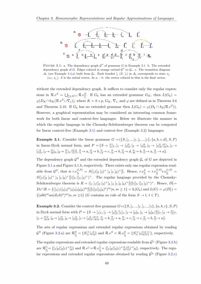
Chapter 3. Homomorphic Representations and Regular Approximations of Languages
Figure 3.1: a. The dependency graph GS of grammar G in Example 3.1. b. The extended
dependency graph of G. Edges colored in orange extend GS to Ge. c. The transition diagram
Ae (see Example 3.4.a) built from Ge. Each bracket [i (S, ]i) in Ae corresponds to state s[i
(sS , s]i). S is the initial vertex. In a. - b. the vertex colored in blue is the final vertex.
without the extended dependency graph. It suffices to consider only the regular expres-
sions in R.eS =⋃
[ti∈N(1) R.eS[ti . If Gk has an extended grammar GK , then L(Gk) =
ϕ(DK ∩hK(R.eS ∪∇e)), where K = k+p, GK , ∇e, and ϕ are defined as in Theorem 3.6
and Theorem 3.10. If Gk has no extended grammar then L(Gk) = ϕ(Dk ∩ hk(R.eS)).
However, a graphical representation may be considered an interesting common frame-
work for both linear and context-free languages. Below we illustrate the manner in
which the regular language in the Chomsky-Schutzenberger theorem can be computed
for linear context-free (Example 3.1) and context-free (Example 3.2) languages.
Example 3.1. Consider the linear grammar G =(S, [1..., [7, ]1..., ]7, a, b, c, d, S, P )
in linear-Dyck normal form, and P = S→ [t1]1, ]1→ [2]t2, [2 → [3]t3, [3 → [2]t2/[t4]4, ]4→
[5]t5, [5→ [t6]6, ]6→ [t1]1/[t7]t7, [
t1→ a, ]t2→ b, ]t3→ c, [t4→ b, ]t5→ d, [t6→ b, [t7→ a, ]t7 → a.
The dependency graph GS and the extended dependency graph Ge of G are depicted in
Figure 3.1.a and Figure 3.1.b, respectively. There exists only one regular expression read-
able from GS , that is r.e(l,S)
[t7= S(]1([2 [3)+ ]4 [5 ]6)+[t7. Hence, r.eS
[t7= r.e
(l,S)
[t7r.e
(r,S)
[t7=
S(]1([2 [3)+ ]4 [5 ]6)+[t7(]5 (]3 ]2)+)+. The regular language provided by the Chomsky-
Schutzenberger theorem is R = ([1 ]1([2 [3)+[4 ]4 [5 [6 ]6)+[t7]t7(]5 (]3 ]2)+)+. Hence, D′7=
D7∩R = ([1]1([2[3)n[4]4[5[6]6)m[t7]t7(]5(]3]2)n)m|n,m ≥ 1 = L(Gk) and L(G) = ϕ(D′7) =
(abb)maa(d(cb)n)m|n,m ≥1 (G contains no rule of the form S → t, t ∈ T ).
Example 3.2. Consider the context-free grammarG=(S, [1..., [7, ]1..., ]7, a, b, c, S, P )
in Dyck normal form with P = S → [1]1, [1 → [5]t5/[1]1, ]1→ [6]6, [2 → [6]6/[t7]7, [3 → [t7]7,
[5→ [t4]t4, [6→ [3]t3, ]6→ [2]t2, ]7→ [3]t3/[t4]t4, ]
t2→ b, ]t3→ a, [t4→ c, ]t4→ c, ]t5→ b, [t7→ a.
The sets of regular expressions and extended regular expressions obtained by reading
GS (Figure 3.2.a) are RS[t4
= S[+1 [5[t4 and R.eS = R.eS[t4
= S[+1 [5[t4]t5]+1 , respectively.
The regular expressions and extended regular expressions readable from G]1 (Figure 3.2.b)
are R]1[t4
= ]1[6([3]7)+[t4 and R.e]1=R.e]1[t4
= ]1[6([3]7)+[t4(]t3)+]6, respectively. The regu-
lar expressions and extended regular expressions obtained by reading G]6 (Figure 3.2.c)
49
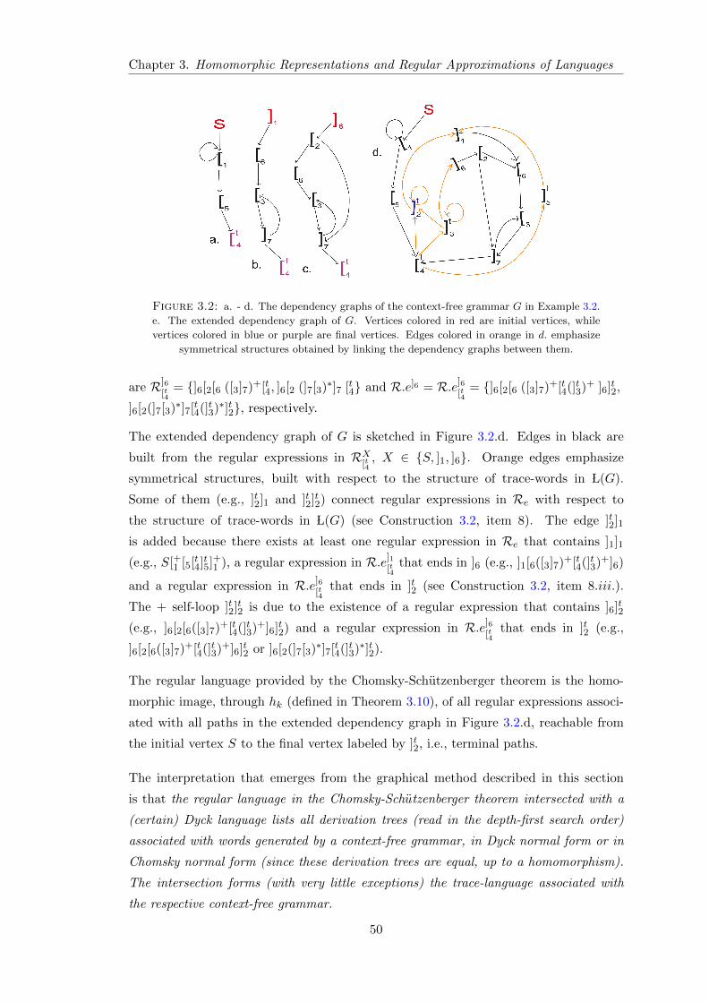
Chapter 3. Homomorphic Representations and Regular Approximations of Languages
Figure 3.2: a. - d. The dependency graphs of the context-free grammar G in Example 3.2.
e. The extended dependency graph of G. Vertices colored in red are initial vertices, while
vertices colored in blue or purple are final vertices. Edges colored in orange in d. emphasize
symmetrical structures obtained by linking the dependency graphs between them.
are R]6[t4
= ]6[2[6 ([3]7)+[t4, ]6[2 (]7[3)∗]7 [t4 and R.e]6 = R.e]6[t4
= ]6[2[6 ([3]7)+[t4(]t3)+ ]6]t2,
]6[2(]7[3)∗]7[t4(]t3)∗]t2, respectively.
The extended dependency graph of G is sketched in Figure 3.2.d. Edges in black are
built from the regular expressions in RX[t4
, X ∈ S, ]1, ]6. Orange edges emphasize
symmetrical structures, built with respect to the structure of trace-words in L(G).
Some of them (e.g., ]t2]1 and ]t2]t2) connect regular expressions in Re with respect to
the structure of trace-words in L(G) (see Construction 3.2, item 8). The edge ]t2]1
is added because there exists at least one regular expression in Re that contains ]1]1
(e.g., S[+1 [5[t4]t5]+1 ), a regular expression in R.e]1[t4
that ends in ]6 (e.g., ]1[6([3]7)+[t4(]t3)+]6)
and a regular expression in R.e]6[t4
that ends in ]t2 (see Construction 3.2, item 8.iii.).
The + self-loop ]t2]t2 is due to the existence of a regular expression that contains ]6]t2
(e.g., ]6[2[6([3]7)+[t4(]t3)+]6]t2) and a regular expression in R.e]6[t4
that ends in ]t2 (e.g.,
]6[2[6([3]7)+[t4(]t3)+]6]t2 or ]6[2(]7[3)∗]7[t4(]t3)∗]t2).
The regular language provided by the Chomsky-Schutzenberger theorem is the homo-
morphic image, through hk (defined in Theorem 3.10), of all regular expressions associ-
ated with all paths in the extended dependency graph in Figure 3.2.d, reachable from
the initial vertex S to the final vertex labeled by ]t2, i.e., terminal paths.
The interpretation that emerges from the graphical method described in this section
is that the regular language in the Chomsky-Schutzenberger theorem intersected with a
(certain) Dyck language lists all derivation trees (read in the depth-first search order)
associated with words generated by a context-free grammar, in Dyck normal form or in
Chomsky normal form (since these derivation trees are equal, up to a homomorphism).
The intersection forms (with very little exceptions) the trace-language associated with
the respective context-free grammar.
50
Chapter 3. Homomorphic Representations and Regular Approximations of Languages
In the next section we refine the extended dependency graph Ge to provide a thiner
regular language in the Chomsky-Schutzenberger theorem with respect to the structure
of the context-free grammar in Dyck normal form obtained through the algorithm de-
scribed in the proof of Theorem 2.15. Based on this readjustment in Section 3.4 we
sketch a transition diagram for a finite automaton and a regular grammar that generates
a regular superset approximation for the initial context-free language.
3.3 Further Refinements of the Regular Language in the
Chomsky-Schutzenberger Theorem
One of the main disadvantage of considering ∗-height regular expressions in building
the extended dependency graph associated with a context-free grammar in Dyck nor-
mal form is that some ∗-loops composed of right brackets in N(2)r ∪ N (3) may not be
symmetrically arranged according to their corresponding left brackets in N(2)r ∪ N (3),
if we consider their corresponding core segment as a symmetrical center. This is due
to the possibility of having “λ-loops”. This deficiency does not affect the intersection
with a Dyck language, but it has the disadvantage of enlarging considerable the regular
language in the Chomsky-Schutzenberger theorem. This can be avoided by considering
only loops described in terms of +-Kleene closure.
Another disfunction of the extended dependency graph built through Construction 3.2 is
the concatenation of a regular expression r.e(l,X)
[tiwith another regular expression r.e
(r,X′)[ti
,
r.e(r,X′)[ti
6= r.e(r,X)
[ti(due to the common tie [ti that marks a core segment). This can be
avoided by a renaming procedure of the regular expressions we want to concatenate.
All these additional modifications in building an extended dependency graph are useful
only if we want to refine the regular language that satisfies the Chomsky-Schutzenberger
theorem (with regards to the grammar in Dyck normal form). This will be further
handled (in Section 3.4) to build a tighter approximation for the context-free language
it characterizes.
Each regular expression of a finite star-height can be described as a finite union of regular
expressions in terms of +-Kleene closure (shortly plus-height). For instance the ∗-height
regular expression ]6[2(]7[3)∗]7[t4 in R]6[t4
can be forked into ]6[2(]7[3)+]7[t4 and ]6[2]7[t4. The
plus-height of a regular expression, can be defined analogous to the star-height of a
regular expression in [98], as follows.
Definition 3.11. Let Σ be a finite alphabet. The plus-height h(r) of a regular expression
r is defined recursively as follows: i. h(λ) = h(∅) = h(a) = 0 for a ∈ Σ, ii. h(r1 ∪ r2) =
h(r1r2) = maxh(r1), h(r2), and h(r+) = h(r) + 1.
51
Chapter 3. Homomorphic Representations and Regular Approximations of Languages
Note that for any star-height regular expression it is possible to build a digraph, with
an initial vertex vi and a final vertex vf , such that all paths in this digraph, from vi to
vf , to provide the respective regular expression (which can be done in a similar manner
as in Construction 3.2). However, if the regular expression is described in terms of plus-
height then this statement may not be true (due to the repetition of some symbols). To
force this statement be true, also for plus-height regular expressions, each repetition of a
bracket is marked by a distinct symbol (e.g., ]6[2(]7[3)+]7[t4 becomes ]6[2(]7[3)+ ]7[t4), and
then, for the new plus-height regular expression obtained in this way, we build a digraph
with the above property. In order to recover the initial plus-height regular expression
from the associated digraph, a homomorphism that maps all the marked brackets (by
distinct symbols) into the initial one must be applied. Each time it is required, we refer
to such a vertex as a ~-marked vertex. Therefore, due to the technical transformations
described above and the symmetrical considerations used in the construction of a trace-
language, we may assume to work only with plus-height regular expressions.
Let Gk = (Nk, T, Pk, S) be an arbitrary context-free grammar in Dyck normal form, and
GX the dependency graph of Gk (see Construction 3.1). Denote by PX[ti
the set of all
plus-height regular expressions over Nk ∪ X that can be read in GX , starting from
the initial vertex X and ending in the final vertex [ti. The cardinality of PX[ti
is finite.
Now, we consider the same homomorphism as defined for the case of the set RX[ti
, i.e.,
hG : Nk∪X → ]i| ]i ∈ N(2)r ∪N (3)∪λ such that hG([i) = ]i for any [i, ]i ∈ N (2)
r ∪N (3),
hG(X) = hG([ti) = hG(]j) = λ, for any [ti ∈ N (1) and ]j ∈ N(2)l . For any element
r.e(l,X)
[ti∈ PX
[tiwe build a new plus-height regular expression r.e
(r,X)
[ti= hrG(r.e
(l,X)
[ti),
where hrG is the mirror image of hG . Consider r.eX[ti
= r.e(l,X)
[tir.e
(r,X)
[ti. For a certain X
and [ti, denote by P.eX[ti
the set of all (plus-height) regular expressions r.eX[ti
obtained as
above. Furthermore, P.eX =⋃
[ti∈N(1) P.eX[ti , and P.e = P.eS ∪ (⋃
]i∈N(3) P.e]i).
Note that linear context-free languages do not need an extended dependency graph. The
set of all regular expressions P.eS suffices to build a regular language in the Chomsky-
Schutzenberger theorem (see Theorem 3.10) that cannot be further adjusted by using the
graphical method proposed in this section. Furthermore, |R.eS | ≤ |P.eS |. Equality takes
place only when each regular expression in R.eS is a plus-height regular expression (see
Example 3.1). For the case of context-free languages the plus-height regular expressions
in P.e must be linked with each other in such a way it approximates, as much as possible,
the trace-language associated with the respective context-free language.
In order to find an optimal connection of the regular expressions in P.e, we consider
the following labeling procedure of elements in P.e. Denote by c0 the cardinality of
P.eS and by cj the cardinality of P.e]j , where ]j ∈ N (3). Each regular expression
r ∈ P.eS is labeled by a unique q, 1 ≤ q ≤ c0, and each regular expression r ∈ P.e]j ,
52
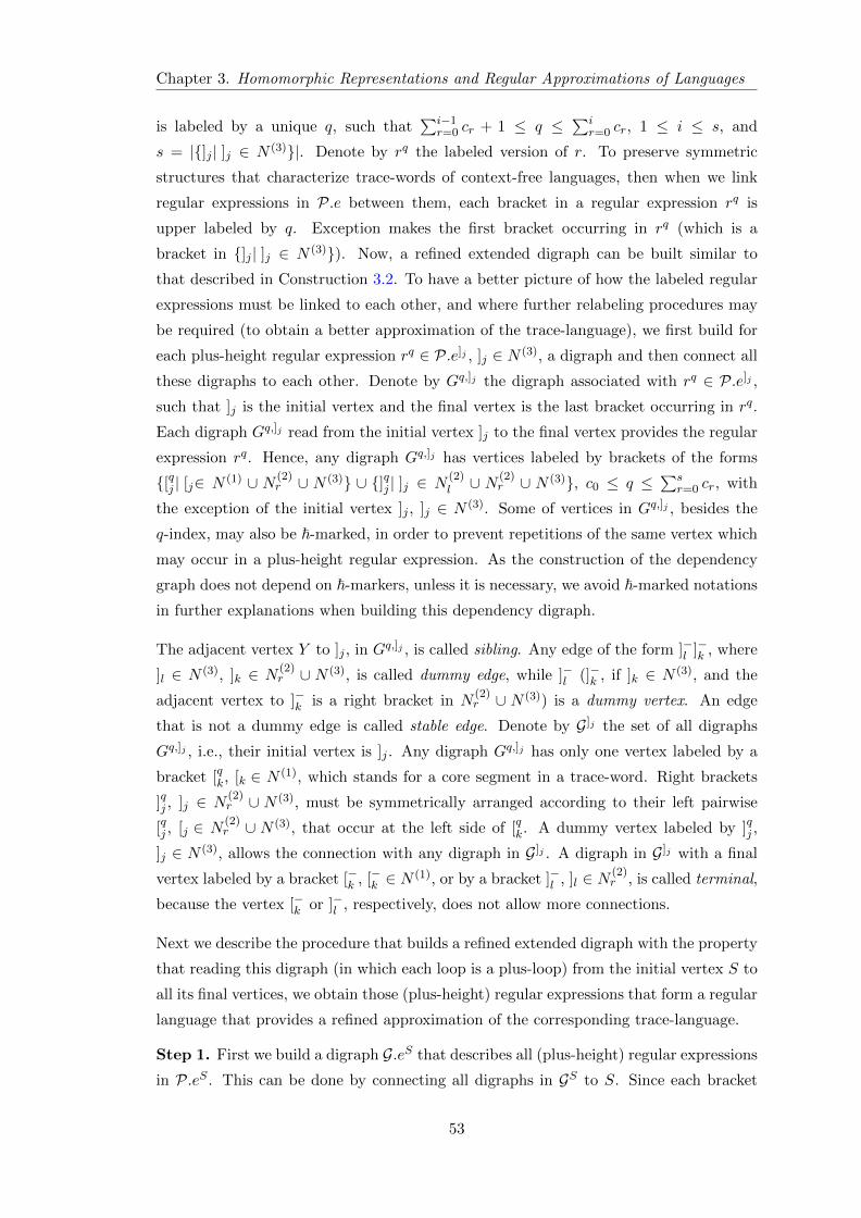
Chapter 3. Homomorphic Representations and Regular Approximations of Languages
is labeled by a unique q, such that∑i−1
r=0 cr + 1 ≤ q ≤∑i
r=0 cr, 1 ≤ i ≤ s, and
s = |]j | ]j ∈ N (3)|. Denote by rq the labeled version of r. To preserve symmetric
structures that characterize trace-words of context-free languages, then when we link
regular expressions in P.e between them, each bracket in a regular expression rq is
upper labeled by q. Exception makes the first bracket occurring in rq (which is a
bracket in ]j | ]j ∈ N (3)). Now, a refined extended digraph can be built similar to
that described in Construction 3.2. To have a better picture of how the labeled regular
expressions must be linked to each other, and where further relabeling procedures may
be required (to obtain a better approximation of the trace-language), we first build for
each plus-height regular expression rq ∈ P.e]j , ]j ∈ N (3), a digraph and then connect all
these digraphs to each other. Denote by Gq,]j the digraph associated with rq ∈ P.e]j ,
such that ]j is the initial vertex and the final vertex is the last bracket occurring in rq.
Each digraph Gq,]j read from the initial vertex ]j to the final vertex provides the regular
expression rq. Hence, any digraph Gq,]j has vertices labeled by brackets of the forms
[qj | [j∈ N (1) ∪ N (2)r ∪ N (3) ∪ ]qj | ]j ∈ N
(2)l ∪ N (2)
r ∪ N (3), c0 ≤ q ≤∑s
r=0 cr, with
the exception of the initial vertex ]j , ]j ∈ N (3). Some of vertices in Gq,]j , besides the
q-index, may also be ~-marked, in order to prevent repetitions of the same vertex which
may occur in a plus-height regular expression. As the construction of the dependency
graph does not depend on ~-markers, unless it is necessary, we avoid ~-marked notations
in further explanations when building this dependency digraph.
The adjacent vertex Y to ]j , in Gq,]j , is called sibling. Any edge of the form ]−l ]−k , where
]l ∈ N (3), ]k ∈ N(2)r ∪ N (3), is called dummy edge, while ]−l (]−k , if ]k ∈ N (3), and the
adjacent vertex to ]−k is a right bracket in N(2)r ∪ N (3)) is a dummy vertex. An edge
that is not a dummy edge is called stable edge. Denote by G]j the set of all digraphs
Gq,]j , i.e., their initial vertex is ]j . Any digraph Gq,]j has only one vertex labeled by a
bracket [qk, [k ∈ N (1), which stands for a core segment in a trace-word. Right brackets
]qj , ]j ∈ N(2)r ∪ N (3), must be symmetrically arranged according to their left pairwise
[qj , [j ∈ N(2)r ∪ N (3), that occur at the left side of [qk. A dummy vertex labeled by ]qj ,
]j ∈ N (3), allows the connection with any digraph in G]j . A digraph in G]j with a final
vertex labeled by a bracket [−k , [−k ∈ N(1), or by a bracket ]−l , ]l ∈ N
(2)r , is called terminal,
because the vertex [−k or ]−l , respectively, does not allow more connections.
Next we describe the procedure that builds a refined extended digraph with the property
that reading this digraph (in which each loop is a plus-loop) from the initial vertex S to
all its final vertices, we obtain those (plus-height) regular expressions that form a regular
language that provides a refined approximation of the corresponding trace-language.
Step 1. First we build a digraph G.eS that describes all (plus-height) regular expressions
in P.eS . This can be done by connecting all digraphs in GS to S. Since each bracket
53
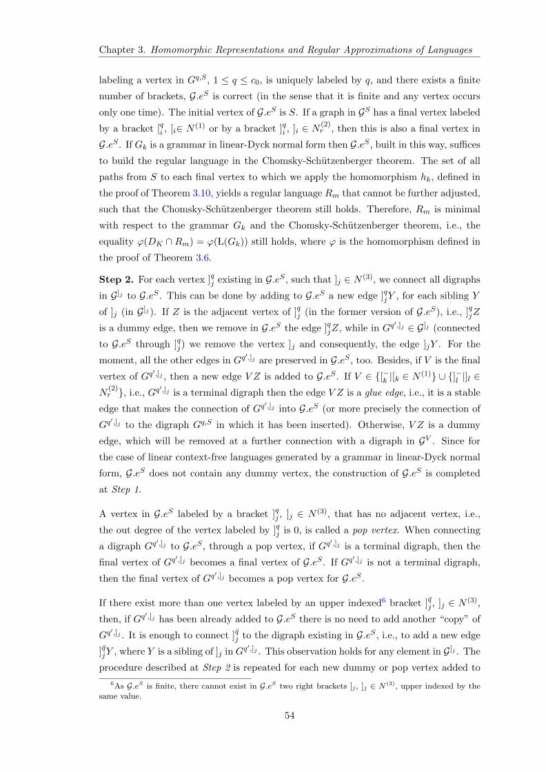
Chapter 3. Homomorphic Representations and Regular Approximations of Languages
labeling a vertex in Gq,S , 1 ≤ q ≤ c0, is uniquely labeled by q, and there exists a finite
number of brackets, G.eS is correct (in the sense that it is finite and any vertex occurs
only one time). The initial vertex of G.eS is S. If a graph in GS has a final vertex labeled
by a bracket [qi , [i∈ N (1) or by a bracket ]qi , ]i ∈ N (2)r , then this is also a final vertex in
G.eS . If Gk is a grammar in linear-Dyck normal form then G.eS , built in this way, suffices
to build the regular language in the Chomsky-Schutzenberger theorem. The set of all
paths from S to each final vertex to which we apply the homomorphism hk, defined in
the proof of Theorem 3.10, yields a regular language Rm that cannot be further adjusted,
such that the Chomsky-Schutzenberger theorem still holds. Therefore, Rm is minimal
with respect to the grammar Gk and the Chomsky-Schutzenberger theorem, i.e., the
equality ϕ(DK ∩ Rm) = ϕ( L(Gk)) still holds, where ϕ is the homomorphism defined in
the proof of Theorem 3.6.
Step 2. For each vertex ]qj existing in G.eS , such that ]j ∈ N (3), we connect all digraphs
in G]j to G.eS . This can be done by adding to G.eS a new edge ]qjY , for each sibling Y
of ]j (in G]j ). If Z is the adjacent vertex of ]qj (in the former version of G.eS), i.e., ]qjZ
is a dummy edge, then we remove in G.eS the edge ]qjZ, while in Gq′,]j ∈ G]j (connected
to G.eS through ]qj) we remove the vertex ]j and consequently, the edge ]jY . For the
moment, all the other edges in Gq′,]j are preserved in G.eS , too. Besides, if V is the final
vertex of Gq′,]j , then a new edge V Z is added to G.eS . If V ∈ [−k |[k ∈ N
(1) ∪ ]−l |]l ∈N
(2)r , i.e., Gq
′,]j is a terminal digraph then the edge V Z is a glue edge, i.e., it is a stable
edge that makes the connection of Gq′,]j into G.eS (or more precisely the connection of
Gq′,]j to the digraph Gq,S in which it has been inserted). Otherwise, V Z is a dummy
edge, which will be removed at a further connection with a digraph in GV . Since for
the case of linear context-free languages generated by a grammar in linear-Dyck normal
form, G.eS does not contain any dummy vertex, the construction of G.eS is completed
at Step 1.
A vertex in G.eS labeled by a bracket ]qj , ]j ∈ N (3), that has no adjacent vertex, i.e.,
the out degree of the vertex labeled by ]qj is 0, is called a pop vertex. When connecting
a digraph Gq′,]j to G.eS , through a pop vertex, if Gq
′,]j is a terminal digraph, then the
final vertex of Gq′,]j becomes a final vertex of G.eS . If Gq
′,]j is not a terminal digraph,
then the final vertex of Gq′,]j becomes a pop vertex for G.eS .
If there exist more than one vertex labeled by an upper indexed6 bracket ]qj , ]j ∈ N (3),
then, if Gq′,]j has been already added to G.eS there is no need to add another “copy” of
Gq′,]j . It is enough to connect ]qj to the digraph existing in G.eS , i.e., to add a new edge
]qjY , where Y is a sibling of ]j in Gq′,]j . This observation holds for any element in G]j . The
procedure described at Step 2 is repeated for each new dummy or pop vertex added to
6As G.eS is finite, there cannot exist in G.eS two right brackets ]j , ]j ∈ N (3), upper indexed by thesame value.
54
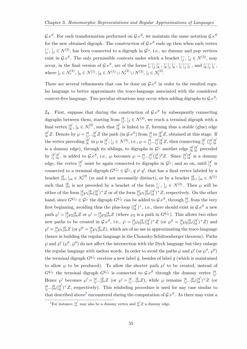
Chapter 3. Homomorphic Representations and Regular Approximations of Languages
G.eS . For each transformation performed on G.eS , we maintain the same notation G.eS
for the new obtained digraph. The construction of G.eS ends up then when each vertex
]−j , ]j ∈ N (3), has been connected to a digraph in G]j , i.e., no dummy and pop vertices
exist in G.eS . The only permissible contexts under which a bracket ]−j , ]j ∈ N (3), may
occur, in the final version of G.eS , are of the forms ]−i ]−j [−k , [−h ]−j [−k , ]−i ]−j ]−l , and [−h ]−j ]−l ,
where ]i ∈ N (2)r , [h ∈ N (1), [k ∈ N (1) ∪N (2)
r ∪N (3), ]l ∈ N(2)l .
There are several refinements that can be done on G.eS in order to the resulted regu-
lar language to better approximate the trace-language associated with the considered
context-free language. Two peculiar situations may occur when adding digraphs to G.eS :
I1. First, suppose that during the construction of G.eS by subsequently connecting
digraphs between them, starting from ]qj , ]j ∈ N (3), we reach a terminal digraph with a
final vertex ]q′
k , ]k ∈ N(2)r , such that ]q
′
k is linked to Z, forming thus a stable (glue) edge
]q′
k Z. Denote by ℘ = ]qj ...]q′
k Z the path (in G.eS) from ]qj to ]q′
k Z, obtained at this stage. If
the vertex preceding ]q′
k in ℘ is ]q′
j , ]j ∈ N (3), i.e., ℘ = ]qj ...]q′
j ]q′
k Z, then connecting ]q′
j (]q′
j ]q′
k
is a dummy edge), through its siblings, to digraphs in G]j another edge ]q′
k ]q′
k preceded
by ]q′
j ]q′
k , is added to G.eS , i.e., ℘ becomes ℘ = ]qj ...]q′
j (]q′
k )2Z. Since ]q′
j ]q′
k is a dummy
edge, the vertex ]q′
j must be again connected to digraphs in G]j , and so on, until ]q′
j is
connected to a terminal digraph Gq,]j ∈ G]j , q 6= q′, that has a final vertex labeled by a
bracket ]qm, ]m ∈ N (2)r (m and k not necessarily distinct), or by a bracket [qm, [m ∈ N (1)
such that ]qm is not preceded by a bracket of the form ]−j , ]j ∈ N (3). Then ℘ will be
either of the form ]qj℘1]qm(]q′
k )+Z or of the form ]qj℘1[qm(]q′
k )+Z, respectively. On the other
hand, since Gq,]j ∈ G]j the digraph Gq,]j can be added to G.eS , through ]qj , from the very
first beginning, avoiding thus the plus-loop (]q′
k )+, i.e., there should exist in G.eS a new
path ℘′ = ]qj℘2]qmZ or ℘′ = ]qj℘2[qmZ (where ℘2 is a path in Gq,]j ). This allows two other
new paths to be created in G.eS , i.e., ℘ = ]qj℘2]qm(]q′
k )+Z (or ℘′′ = ]qj℘2[qm(]q′
k )+Z) and
℘′ = ]qj℘1]qmZ (or ℘′′ = ]qj℘1[qmZ), which are of no use in approximating the trace-language
(hence in building the regular language in the Chomsky-Schutzenberger theorem). Paths
℘ and ℘′ (℘′′, ℘′′) do not affect the intersection with the Dyck language but they enlarge
the regular language with useless words. In order to avoid the paths ℘ and ℘′ (or ℘′′, ℘′′)
the terminal digraph Gq,]j receives a new label q, besides of label q (which is maintained
to allow ℘ to be produced). To allow the shorter path ℘′ to be created, instead of
Gq,]j the terminal digraph Gq,]j is connected to G.eS through the dummy vertex ]qj .
Hence ℘′ becomes ℘′ = ]qj ...]qmZ (or ℘′ = ]qj ...[
qmZ), while ℘ remains ]qj ...]
qm(]q
′
k )+Z (or
]qj ...[qm(]q
′
k )+Z, respectively). This relabeling procedure is used for any case similar to
that described above7 encountered during the computation of G.eS . As there may exist a
7For instance, ]q′
k may also be a dummy vertex and ]q′
k Z a dummy edge.
55
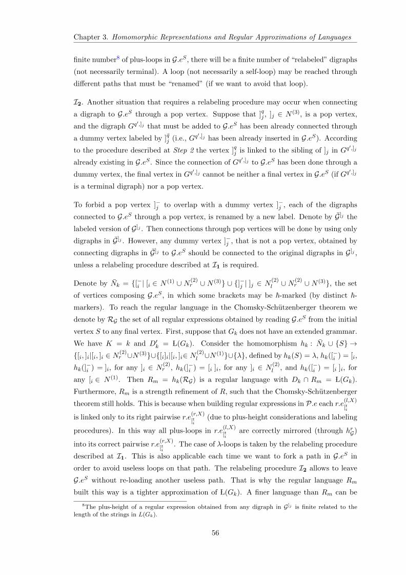
Chapter 3. Homomorphic Representations and Regular Approximations of Languages
finite number8 of plus-loops in G.eS , there will be a finite number of “relabeled” digraphs
(not necessarily terminal). A loop (not necessarily a self-loop) may be reached through
different paths that must be “renamed” (if we want to avoid that loop).
I2. Another situation that requires a relabeling procedure may occur when connecting
a digraph to G.eS through a pop vertex. Suppose that ]qj , ]j ∈ N (3), is a pop vertex,
and the digraph Gq′,]j that must be added to G.eS has been already connected through
a dummy vertex labeled by ]qj (i.e., Gq′,]j has been already inserted in G.eS). According
to the procedure described at Step 2 the vertex ]qj is linked to the sibling of ]j in Gq′,]j
already existing in G.eS . Since the connection of Gq′,]j to G.eS has been done through a
dummy vertex, the final vertex in Gq′,]j cannot be neither a final vertex in G.eS (if Gq
′,]j
is a terminal digraph) nor a pop vertex.
To forbid a pop vertex ]−j to overlap with a dummy vertex ]−j , each of the digraphs
connected to G.eS through a pop vertex, is renamed by a new label. Denote by G]j the
labeled version of G]j . Then connections through pop vertices will be done by using only
digraphs in G]j . However, any dummy vertex ]−j , that is not a pop vertex, obtained by
connecting digraphs in G]j to G.eS should be connected to the original digraphs in G]j ,
unless a relabeling procedure described at I1 is required.
Denote by Nk = [−i | [i ∈ N (1) ∪ N (2)r ∪ N (3) ∪ ]−j | ]j ∈ N
(2)l ∪ N (2)
r ∪ N (3), the set
of vertices composing G.eS , in which some brackets may be ~-marked (by distinct ~-
markers). To reach the regular language in the Chomsky-Schutzenberger theorem we
denote by RG the set of all regular expressions obtained by reading G.eS from the initial
vertex S to any final vertex. First, suppose that Gk does not have an extended grammar.
We have K = k and D′k = L(Gk). Consider the homomorphism hk : Nk ∪ S →[i, ]i|[i, ]i ∈ N (2)
r ∪N (3)∪[i]i|[i, ]i∈ N (2)l ∪N
(1)∪λ, defined by hk(S) = λ, hk([−i ) = [i,
hk(]−i ) = ]i, for any ]i ∈ N (2)
r , hk(]−i ) = [i ]i, for any ]i ∈ N (2)
l , and hk([−i ) = [i ]i, for
any [i ∈ N (1). Then Rm = hk(RG) is a regular language with Dk ∩ Rm = L(Gk).
Furthermore, Rm is a strength refinement of R, such that the Chomsky-Schutzenberger
theorem still holds. This is because when building regular expressions in P.e each r.e(l,X)
[ti
is linked only to its right pairwise r.e(r,X)
[ti(due to plus-height considerations and labeling
procedures). In this way all plus-loops in r.e(l,X)
[tiare correctly mirrored (through hrG)
into its correct pairwise r.e(r,X)
[ti. The case of λ-loops is taken by the relabeling procedure
described at I1. This is also applicable each time we want to fork a path in G.eS in
order to avoid useless loops on that path. The relabeling procedure I2 allows to leave
G.eS without re-loading another useless path. That is why the regular language Rm
built this way is a tighter approximation of L(Gk). A finer language than Rm can be
8The plus-height of a regular expression obtained from any digraph in G]j is finite related to thelength of the strings in L(Gk).
56
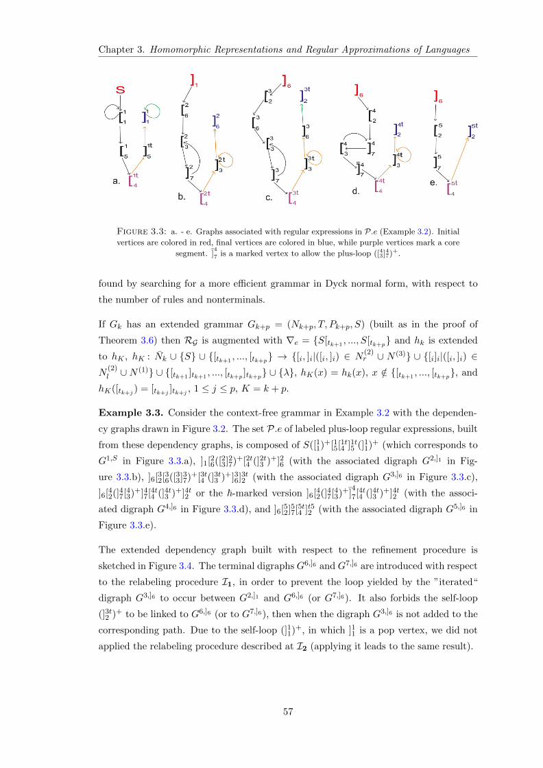
Chapter 3. Homomorphic Representations and Regular Approximations of Languages
Figure 3.3: a. - e. Graphs associated with regular expressions in P.e (Example 3.2). Initial
vertices are colored in red, final vertices are colored in blue, while purple vertices mark a core
segment. ]4
7 is a marked vertex to allow the plus-loop ([43]47)+.
found by searching for a more efficient grammar in Dyck normal form, with respect to
the number of rules and nonterminals.
If Gk has an extended grammar Gk+p = (Nk+p, T, Pk+p, S) (built as in the proof of
Theorem 3.6) then RG is augmented with ∇e = S[tk+1, ..., S[tk+p
and hk is extended
to hK , hK : Nk ∪ S ∪ [tk+1, ..., [tk+p
→ [i, ]i|([i, ]i) ∈ N(2)r ∪ N (3) ∪ [i]i|([i, ]i) ∈
N(2)l ∪ N (1) ∪ [tk+1
]tk+1, ..., [tk+p
]tk+p ∪ λ, hK(x) = hk(x), x /∈ [tk+1
, ..., [tk+p, and
hK([tk+j) = [tk+j
]tk+j, 1 ≤ j ≤ p, K = k + p.
Example 3.3. Consider the context-free grammar in Example 3.2 with the dependen-
cy graphs drawn in Figure 3.2. The set P.e of labeled plus-loop regular expressions, built
from these dependency graphs, is composed of S([11)+[15[1t4 ]1t5 (]11)+ (which corresponds to
G1,S in Figure 3.3.a), ]1[26([23]27)+[2t4 (]2t3 )+]26 (with the associated digraph G2,]1 in Fig-
ure 3.3.b), ]6[32[36([33]37)+[3t4 (]3t3 )+]36]3t2 (with the associated digraph G3,]6 in Figure 3.3.c),
]6[42(]47[43)+]47[4t4 (]4t3 )+]4t2 or the ~-marked version ]6[42(]47[43)+ ]47[4t4 (]4t3 )+]4t2 (with the associ-
ated digraph G4,]6 in Figure 3.3.d), and ]6[52]57[5t4 ]t52 (with the associated digraph G5,]6 in
Figure 3.3.e).
The extended dependency graph built with respect to the refinement procedure is
sketched in Figure 3.4. The terminal digraphs G6,]6 and G7,]6 are introduced with respect
to the relabeling procedure I1, in order to prevent the loop yielded by the ”iterated“
digraph G3,]6 to occur between G2,]1 and G6,]6 (or G7,]6). It also forbids the self-loop
(]3t2 )+ to be linked to G6,]6 (or to G7,]6), then when the digraph G3,]6 is not added to the
corresponding path. Due to the self-loop (]11)+, in which ]11 is a pop vertex, we did not
applied the relabeling procedure described at I2 (applying it leads to the same result).
57
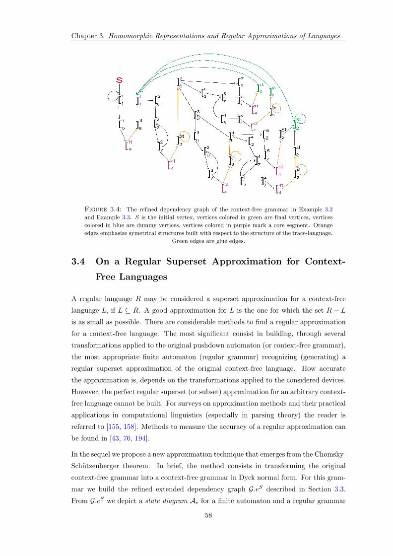
Chapter 3. Homomorphic Representations and Regular Approximations of Languages
Figure 3.4: The refined dependency graph of the context-free grammar in Example 3.2
and Example 3.3. S is the initial vertex, vertices colored in green are final vertices, vertices
colored in blue are dummy vertices, vertices colored in purple mark a core segment. Orange
edges emphasize symetrical structures built with respect to the structure of the trace-language.
Green edges are glue edges.
3.4 On a Regular Superset Approximation for Context-
Free Languages
A regular language R may be considered a superset approximation for a context-free
language L, if L ⊆ R. A good approximation for L is the one for which the set R − Lis as small as possible. There are considerable methods to find a regular approximation
for a context-free language. The most significant consist in building, through several
transformations applied to the original pushdown automaton (or context-free grammar),
the most appropriate finite automaton (regular grammar) recognizing (generating) a
regular superset approximation of the original context-free language. How accurate
the approximation is, depends on the transformations applied to the considered devices.
However, the perfect regular superset (or subset) approximation for an arbitrary context-
free language cannot be built. For surveys on approximation methods and their practical
applications in computational linguistics (especially in parsing theory) the reader is
referred to [155, 158]. Methods to measure the accuracy of a regular approximation can
be found in [43, 76, 194].
In the sequel we propose a new approximation technique that emerges from the Chomsky-
Schutzenberger theorem. In brief, the method consists in transforming the original
context-free grammar into a context-free grammar in Dyck normal form. For this gram-
mar we build the refined extended dependency graph G.eS described in Section 3.3.
From G.eS we depict a state diagram Ae for a finite automaton and a regular grammar
58
Chapter 3. Homomorphic Representations and Regular Approximations of Languages
Gr = (Nr, T, Pr, S) that generates a regular (superset) approximation for L(Gk) (which
is nothing else than the image through ϕ of the language Rm built in Section 3.3).
Let Gk = (Nk, T, Pk, S) be an arbitrary context-free grammar in Dyck normal form,
and G.eS = (Ve, Ee) the extended dependency graph of Gk. Recall that Ve = [−i |[i ∈N (1) ∪N (2)
r ∪N (3) ∪ ]−j |]j ∈ N(2)l ∪N (2)
r ∪N (3) ∪ S in which some of the vertices
may be ~-marked, in order to prevent repetition of the same bracket when building the
digraph associated with a plus-height regular expression. In brief, the state diagram Aecan be built by skipping in G.eS all left brackets in N
(2)r and all brackets in N (3), and
labeling the edges with the symbol produced by left or right bracket in N (2)∪N (1). This
reasoning is applied no matter whether the vertex in Ve is ~-marked or not. Therefore, we
avoid ~-marker specifications when building Ae, unless this is strictly necessary. Denote
by sf the accepting state of Ae. The start state of Ae is sS , where S is the axiom of Gk.
We proceed as follows:
1. There exists an edge inAe from sS to s]qi, labeled by a, where ]i ∈ N (2)
l and [i → a ∈ Pk,if either S]qi ∈ Ee or there exists a path in G.eS from S to ]qi that contains no vertex
labeled by ]qj , ]j ∈ N (2)l , or by [−tk , [k ∈ N (1). We fix S → a]qi ∈ Pr.
2. There exists an edge in Ae from sS to s[qti, labeled by a, and an edge from s[qti
to s]qti
labeled by b, where [ti, ]ti ∈ N (1), [ti → a, and ]ti → b ∈ Pk, if either S[qti ∈ Ee or there
exists a path in G.eS from S to [qti that contains no vertex labeled by ]qj , ]j ∈ N (2)l , or
labeled by [−tk , [k ∈ N (1). We fix S → a[qti , [qti → b]qti ∈ Pr.
3. There exists an edge in Ae from s]qito s]qj
, labeled by a, where ]i, ]j ∈ N(2)l and
[j → a ∈ Pk, if either ]qi ]qj ∈ Ee or there exists a path in G.eS from ]qi to ]qj that contains
no vertex labeled by [qtk or by ]ql , [k ∈ N (1), ]l ∈ N(2)l . If i = j, i.e., ]qi ]
qi is a self-loop in
G.eS , then s]qis]qi
is a self-loop9 in Ae. We fix ]qi → a]qj ∈ Pr.
4. There exists an edge in Ae from s]qito s[qtj
, labeled by a and an edge from s[qtjto s]qtj
labeled by b, where ]i ∈ N (2)l , [j , ]j ∈ N (1), [tj → a, and ]tj → b ∈ Pk, if either ]qi [
qtj ∈ Ee or
there exists a path in G.eS from ]qi to [qtj that contains no vertex labeled by ]qk, ]k ∈ N(2)l .
We fix ]qi → a[qtj , [qtj → b]qtj ∈ Pr.
5. There exists an edge in Ae from s]qito s
]q′j
, labeled by a, where ]i, ]j ∈ N(2)r , and
]j → a ∈ Pk, if ]qi ]q′
j ∈ Ee. If i = j and q = q′, then s]qis]qi
is a self-loop in Ae (because ]qi ]qi
is a self-loop in G.eS). We fix ]qi → a]q′
j ∈ Pr. Note that, it is also possible to have i 6= j
and q = q′ or q 6= q′ (with i = j or i 6= j, case in which ]q−]q′
− is a glue edge in G.eS).
9This case deals also with the situation when ]qi , ]i ∈ N (2)l , occurs in a loop in G.eS composed of only
left brackets in N(2)r ∪N (3), excepting ]qi . A loop composed of only left brackets in N
(2)r ∪N (3) is ignored
when building Ae.
59
Chapter 3. Homomorphic Representations and Regular Approximations of Languages
6. There exists an edge in Ae from s]qito s
]q′j
, labeled by a, where ]i ∈ N (2)r , ]j ∈ N (2)
l ,
and [j → a ∈ Pk, if there exists a path in G.eS from ]qi to ]q′
j that contains no vertex
labeled by ]−k , ]k ∈ N(2)l ∪N
(2)r , or labeled by [−tl , [l ∈ N (1). We fix ]qi → a]q
′
j ∈ Pr. Note
that, q may be equal to q′.
7. There exists an edge s]qis
[q′tj
labeled by a, and an edge s[q′tj
s]q′tj
labeled by b, where
]i ∈ N (2)r , [j , ]j ∈ N (1), [tj → a, and ]tj → b ∈ Pk, if there exists a path in G.eS from ]qi to
[q′tj that contains no vertex labeled by ]−k , ]k ∈ N
(2)l ∪N (2)
r , or by [−tl , [l ∈ N (1). We fix
]qi → a[q′tj , [q
′tj → b]q
′tj ∈ Pr.
8. There exists an edge in Ae from s]qtito s
]q′j
, labeled by a, where [i ∈ N (1), ]j ∈ N (2)r ,
and ]j → a ∈ Pk, if [qti ]q′
j ∈ Ee. We fix ]qti → a]qj ∈ Pr. Note that, it is possible to have
q = q′ or q 6= q′ (in the last case ]qti ]q′
j is a glue edge in G.eS).
9. There exists an edge s]qtis
[q′tj
, labeled by a, and an edge s[q′tj
s]q′tj
labeled by b, where
]i, [j ∈ N (1), [tj → a, and ]tj → b ∈ Pk, if there exists a path in G.eS from [qti to [q′tj
that contains no vertex labeled by ]−k , ]k ∈ N(2)l ∪ N (2)
r , or by [−tl , [l ∈ N (1). We fix
]qti → a[q′tj , [q
′tj → b]q
′tj ∈ Pr. Note that, [qti may be equal to [q
′tj , i.e., i = j and q = q′, i.e.,
the case of a loop in [qti .
10. For any final vertex labeled by ]qi , ]i ∈ N (2)r , or by [qti , [ti ∈ N (1), in G.eS , we add in
Ae a new edge s]qisf , or s]qti
sf , respectively. In both cases, this is labeled by λ. We set
in Pr a rule of the form ]qi → λ or ]qti → λ, respectively.
The new grammar Gr = (Nr, T, Pr, S), in which the set of rules Pr is built as above, and
Nr = ]−i | ]i ∈ N (2) ∪ [−i , ]−i |[i, ]i ∈ N (1) is a regular grammar generating a regular
superset approximation for L(Gk). Recall that some of the brackets in Nr may also be
~-marked (by distinct symbols). It is easy to observe that L(Gr) = ϕ(Rm), where ϕ is
the homomorphism in the proof of Theorem 3.6.
Note that since the regular language in the Chomsky-Schutzenberger theorem is an ap-
proximation of the trace-language, Rm depends on the considered context-free grammar
in Dyck normal form. As for L = L(Gk) there exist several other grammars generating
it, setting these grammars in Dyck normal form other trace-languages can be drawn, and
consequently other regular languages, of type Rm, can be built. The best approximation
for L is the regular language with fewer words that are not in L.
Denote by GL the set of grammars in Dyck normal form generating L, by Rm the set of
all regular languages obtained from the refined extended dependency graphs associated
with grammars in GL, and by AL = ϕ(Rm)|Rm ∈ Rm the set of all superset regular
approximations of L. It is easy to observe that AL, with the inclusion relation on sets,
is a partially ordered subset of context-free languages. AL has an infimum equal to the
60
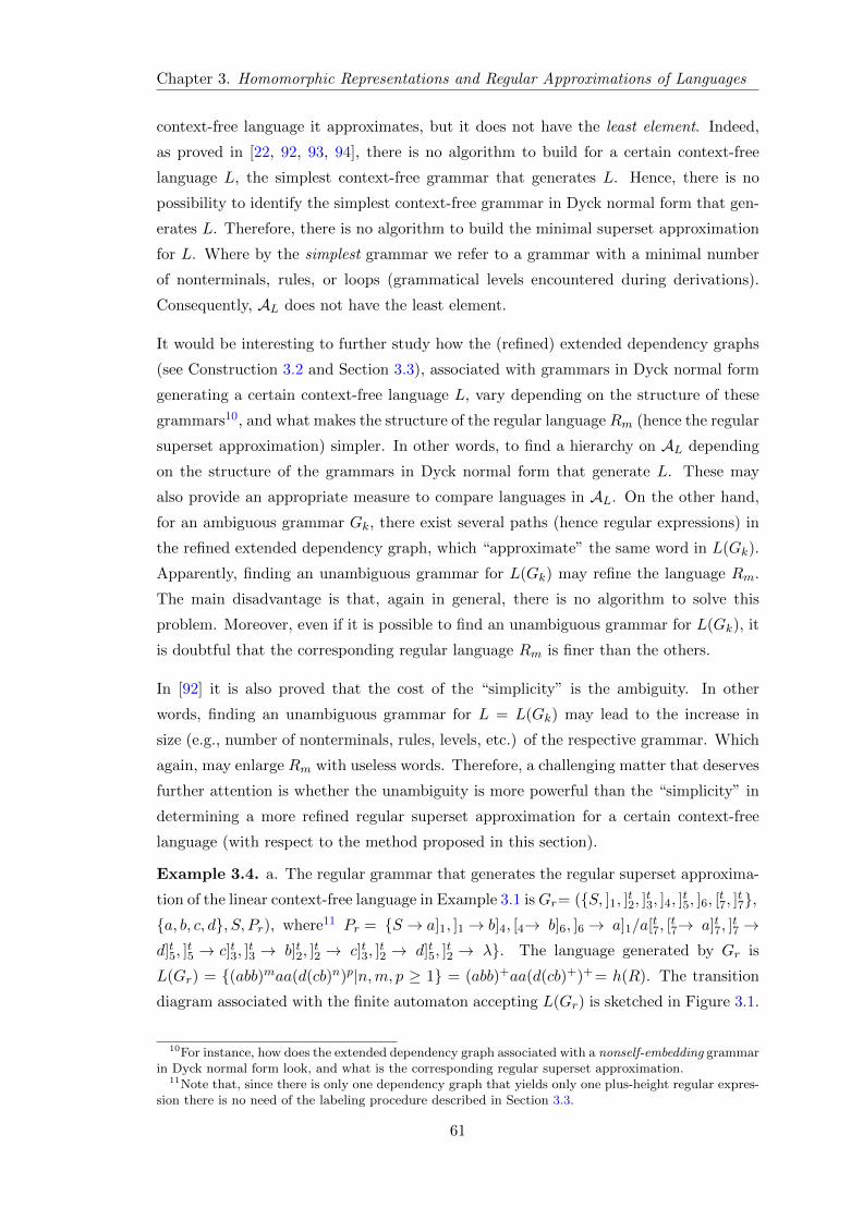
Chapter 3. Homomorphic Representations and Regular Approximations of Languages
context-free language it approximates, but it does not have the least element. Indeed,
as proved in [22, 92, 93, 94], there is no algorithm to build for a certain context-free
language L, the simplest context-free grammar that generates L. Hence, there is no
possibility to identify the simplest context-free grammar in Dyck normal form that gen-
erates L. Therefore, there is no algorithm to build the minimal superset approximation
for L. Where by the simplest grammar we refer to a grammar with a minimal number
of nonterminals, rules, or loops (grammatical levels encountered during derivations).
Consequently, AL does not have the least element.
It would be interesting to further study how the (refined) extended dependency graphs
(see Construction 3.2 and Section 3.3), associated with grammars in Dyck normal form
generating a certain context-free language L, vary depending on the structure of these
grammars10, and what makes the structure of the regular language Rm (hence the regular
superset approximation) simpler. In other words, to find a hierarchy on AL depending
on the structure of the grammars in Dyck normal form that generate L. These may
also provide an appropriate measure to compare languages in AL. On the other hand,
for an ambiguous grammar Gk, there exist several paths (hence regular expressions) in
the refined extended dependency graph, which “approximate” the same word in L(Gk).
Apparently, finding an unambiguous grammar for L(Gk) may refine the language Rm.
The main disadvantage is that, again in general, there is no algorithm to solve this
problem. Moreover, even if it is possible to find an unambiguous grammar for L(Gk), it
is doubtful that the corresponding regular language Rm is finer than the others.
In [92] it is also proved that the cost of the “simplicity” is the ambiguity. In other
words, finding an unambiguous grammar for L = L(Gk) may lead to the increase in
size (e.g., number of nonterminals, rules, levels, etc.) of the respective grammar. Which
again, may enlarge Rm with useless words. Therefore, a challenging matter that deserves
further attention is whether the unambiguity is more powerful than the “simplicity” in
determining a more refined regular superset approximation for a certain context-free
language (with respect to the method proposed in this section).
Example 3.4. a. The regular grammar that generates the regular superset approxima-
tion of the linear context-free language in Example 3.1 isGr= (S, ]1, ]t2, ]t3, ]4, ]t5, ]6, [t7, ]t7,a, b, c, d, S, Pr), where11 Pr = S → a]1, ]1→ b]4, [4→ b]6, ]6→ a]1/a[t7, [
t7→ a]t7, ]
t7→
d]t5, ]t5 → c]t3, ]
t3 → b]t2, ]
t2 → c]t3, ]
t2 → d]t5, ]
t2 → λ. The language generated by Gr is
L(Gr) = (abb)maa(d(cb)n)p|n,m, p ≥ 1 = (abb)+aa(d(cb)+)+ = h(R). The transition
diagram associated with the finite automaton accepting L(Gr) is sketched in Figure 3.1.
10For instance, how does the extended dependency graph associated with a nonself-embedding grammarin Dyck normal form look, and what is the corresponding regular superset approximation.
11Note that, since there is only one dependency graph that yields only one plus-height regular expres-sion there is no need of the labeling procedure described in Section 3.3.
61
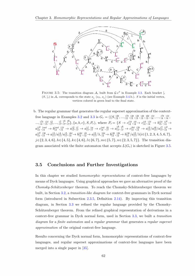
Chapter 3. Homomorphic Representations and Regular Approximations of Languages
Figure 3.5: The transition diagram Ae built from G.eS in Example 3.3. Each bracket [i(S, ]i) in Ae corresponds to the state s[i (sS , s]i) (see Example 3.4.b.). S is the initial vertex,
vertices colored in green lead to the final state.
b. The regular grammar that generates the regular superset approximation of the context-
free language in Examples 3.2 and 3.3 is Gr = (S, ]3t2 , ..., ]7t2 , ]2t3 , ]3t3 , ]4t3 , ]6t3 , [1t4 , ..., [7t4 , ]1t4 ,..., ]7t4 , ]
1t5 , ]
27, ..., ]
77, ]
47, ]
67, a, b, c, S, Pr), where Pr= S → c[1t4 , [
it4→ c]it4 , ]
1t4 → b]1t5 , ]
jt4 →
a]jt3 , ]mt4 → b]mt2 , ]1t5 → a]27, ]
j7 → a]j7, ]
n7 → c[nt4 , ]
k7 → a]
k7, ]
k7 → c[kt4 , ]
2t3 → a]37/a]67/a]77, ]
jt3 →
a]jt3 , ]3t3 → a]37/a]47/a]57, ]
kt3 → b]kt2 , ]
lt2→ a]27/λ, ]
ht2 → b]3t2 , ]
3t2 → b]3t2 /a]27/λ|i∈1, 2, 3, 4, 5, 6, 7,
j∈2, 3, 4, 6, h∈4, 5, k∈4, 6, l∈6, 7,m∈5, 7, n∈2, 3, 5, 7. The transition dia-
gram associated with the finite automaton that accepts L(Gr) is sketched in Figure 3.5.
3.5 Conclusions and Further Investigations
In this chapter we studied homomorphic representations of context-free languages by
means of Dyck languages. Using graphical approaches we gave an alternative proof of the
Chomsky-Schutzenberger theorem. To reach the Chomsky-Schutzenberger theorem we
built, in Section 3.2, a transition-like diagram for context-free grammars in Dyck normal
form (introduced in Subsection 2.3.5, Definition 2.14). By improving this transition
diagram, in Section 3.3 we refined the regular language provided by the Chomsky-
Schutzenberger theorem. From the refined graphical representation of derivations in a
context-free grammar in Dyck normal form, used in Section 3.3, we built a transition
diagram for a finite automaton and a regular grammar that generates a regular superset
approximation of the original context-free language.
Results concerning the Dyck normal form, homomorphic representations of context-free
languages, and regular superset approximations of context-free languages have been
merged into a single paper in [35].
62
Chapter 3. Homomorphic Representations and Regular Approximations of Languages
A challenging problem for further investigations may be to further refine this superset
approximation depending on the type of the grammar (e.g. nonself-embedding or un-
ambiguous) or on the size of the grammar (e.g. number of nonterminals, rules, etc.)
generating a certain context-free language. In [43] it is proved that optimal (minimal)
superset approximations exist for several kind of context-free languages, but no specifi-
cation is provided of how the existing minimal approximation can be built starting from
the context-free language it approximates. It would be challenging to further investigate
whether there exist subsets of context-free languages for which it would be possible to
build a minimal superset approximation (by using the graphical method proposed in
this chapter).
The method used throughout this chapter is graphically constructive, and it shows that i.
derivational structures in context-free grammars can be better described through nested
systems of parenthesis (Dyck languages), and ii. the Chomsky-Schutzenberger theorem
may render a good and efficient approximation for context-free languages. Furthermore,
the method provides a graphical framework to handle derivations and descriptional struc-
tures in context-free grammars, which may be useful in further complexity investigations
of context-free languages.
63
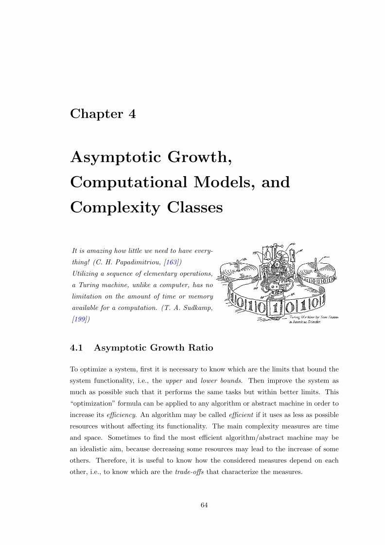
Chapter 4
Asymptotic Growth,
Computational Models, and
Complexity Classes
It is amazing how little we need to have every-
thing! (C. H. Papadimitriou, [163])
Utilizing a sequence of elementary operations,
a Turing machine, unlike a computer, has no
limitation on the amount of time or memory
available for a computation. (T. A. Sudkamp,
[199])
4.1 Asymptotic Growth Ratio
To optimize a system, first it is necessary to know which are the limits that bound the
system functionality, i.e., the upper and lower bounds. Then improve the system as
much as possible such that it performs the same tasks but within better limits. This
“optimization” formula can be applied to any algorithm or abstract machine in order to
increase its efficiency. An algorithm may be called efficient if it uses as less as possible
resources without affecting its functionality. The main complexity measures are time
and space. Sometimes to find the most efficient algorithm/abstract machine may be
an idealistic aim, because decreasing some resources may lead to the increase of some
others. Therefore, it is useful to know how the considered measures depend on each
other, i.e., to know which are the trade-offs that characterize the measures.
64
Chapter 4. Asymptotic Growth, Computational Models, and Complexity Classes
The main tool used to achieve the above goals is the so called asymptotic analysis,
which investigates how the amount of resources spent by an algorithm (or an abstract
machine) grows as a function of the size of the input, as the size of the input approaches
infinity. If the corresponding function is unintuitive, such as a sum or a product of
several elementary functions, in terms of the input size, an asymptotic approximation
of the initial function, in terms of the most appropriate function concerning the order
of magnitude, is required.
For surveys and applications of asymptotic analysis in computer science, especially in
analysis of algorithms and complexity classes, the reader is referred to [44, 86, 125].
There are three types of asymptotic approximations, usually called asymptotic notations,
asymptotic upper bounds provided by O(·) and o(·) notations, asymptotic lower bounds
provided by Ω(·) and ω(·) notations, and asymptotic equivalence relation provided by
Θ(·) notation.
4.1.1 Asymptotic Upper Bounds
An asymptotic upper bound is an approximation of a function in terms of the most
appropriate function of the same or greater magnitude. Formally, we have
Definition 4.1. Let f, g : N→ R be two functions.
- We say that f(n) is big-O of g(n), denoted by f(n) = O(g(n)), if and only if there
exist two positive constants c and n0 such that |f(n)| ≤ c|g(n)|, for all n ≥ n0.
- We say that f(n) is small-o of g(n), denoted by f(n) = o(g(n)), if and only if for any
positive constant c there exists a positive constant n0 such that |f(n)| ≤ c|g(n)|, for all
n ≥ n0.
Remarks 1. f(n) = O(g(n)) means that f(n) is a member of the set O(g(n)) which
is composed of all functions asymptotically upper bounded by g(n). In other words,
O(g(n)) is composed of functions of equal, within a constant factor, or smaller magnitude
than g(n), as n approaches infinity. In terms of limit operation1, if limn→∞
∣∣∣f(n)g(n)
∣∣∣ < ∞then f(n) = O(g(n)). The O(·) notation allows asymptotic upper approximations of
f(n) in terms of a function of the same or greater magnitude, multiplied by a constant
factor. Hence, O(1) is the set of at most constant growth functions, O(log n) is the
set of at most logarithmic growth functions, O(n) is the set of at most linear growth
functions, O(nc), c ≥ 1, is the set of polynomial growth functions, while O(cn), c ≥ 1,
is the set of exponentially growing functions, and so on. The next hierarchy hold:
... ⊂ O( 12n ) ⊂ O( 1
n) ⊂ O(1) ⊂ O(log log n) ⊂ O(log n) ⊂ O(√n) ⊂ O(n) ⊂ O(n log n) ⊂
1Recall that the converse does not hold. A counter example can be provided by the functions g(n) = nand f(n) = n sinn. Clearly, n sinn ∈ O(n), but lim
n→∞
∣∣n sinnn
∣∣ = limn→∞
| sinn| does not exist.
65
Chapter 4. Asymptotic Growth, Computational Models, and Complexity Classes
O(nc) ⊂ O(cn) ⊂ O(n!) ⊂ O(nn) ⊂ O(22n) ⊂ ..., which certainly can be enriched with
infinitely many other classes.
2. f(n) = o(g(n)) means that f(n) is a member of the set o(g(n)) which is composed
of all functions asymptotically strict upper bounded by g(n), as n approaches infinity,
i.e., limn→∞
∣∣∣f(n)g(n)
∣∣∣ = 0 if and only if f(n) = o(g(n)). The o(·) notation allows asymptotic
upper approximations of f(n) in terms of functions of greater magnitude than f(n).
3. o(g(n)) ⊂ O(g(n)).
4.1.2 Asymptotic Lower Bounds
An asymptotic lower bound is an approximation of a function in terms of the most
appropriate function of the same or lower magnitude. Formally, we have
Definition 4.2. Let f, g : N→ R be two functions.
- We say that f(n) is big-Ω of g(n), denoted by f(n) = Ω(g(n)), if and only if there exist
two positive constants c and n0 such that |f(n)| ≥ c|g(n)|, for all n ≥ n0.
- We say that f(n) is small-ω of g(n), denoted by f(n) = ω(g(n)), if and only if for any
positive constant c there exists a positive constant n0 such that |f(n)| ≥ c|g(n)|, for all
n ≥ n0.
Remarks 1. f(n) = Ω(g(n)) means that f(n) is a member of the set Ω(g(n)) which is
composed of all functions asymptotically lower bounded by g(n). In other words, Ω(g(n))
is composed of functions of equal, within a constant factor, or greater magnitude than
g(n), as n approaches infinity. In terms of limit operation, if limn→∞
∣∣∣f(n)g(n)
∣∣∣ > 0 then
f(n) = Ω(g(n)). The Ω(·) notation allows asymptotic lower approximations of f(n) in
terms of a function of the same or lower magnitude, multiplied by a constant factor.
2. f(n) = ω(g(n)) means that f(n) is a member of the set ω(g(n)) which is composed
of all functions asymptotically strict lower bounded by g(n), as n approaches infinity,
i.e., limn→∞
∣∣∣f(n)g(n)
∣∣∣ =∞ if and only if f(n) = ω(g(n)). The ω(·) notation allows asymptotic
lower approximations of f(n) in terms of functions of smaller magnitude than f(n).
3. ω(g(n)) ⊂ Ω(g(n)) and ω(g(n)) ∩ O(g(n)) = ∅.
4.1.3 Asymptotic Equivalence
Definition 4.3. Let f, g : N→ R be two functions. We say that f(n) is big-Θ of g(n),
denoted by f(n) = Θ(g(n)), if and only if there exist three positive constants c1, c2, and
n0 such that c1|g(n)| ≤ |f(n)| ≤ c2|g(n)|, for all n ≥ n0.
66
Chapter 4. Asymptotic Growth, Computational Models, and Complexity Classes
Remarks 1. f(n) = Θ(g(n)) means that f(n) grows at the same rate as g(n), and that
f(n) is a member of the set Θ(g(n)) which is composed of all functions asymptotically
equivalent to g(n), i.e., functions of equal magnitude as g(n), within some constant
factors. In terms of limits, if 0 < limn→∞
∣∣∣f(n)g(n)
∣∣∣ < ∞ then f(n) = Θ(g(n)). The Θ(·)notation allows in the same time asymptotic lower and upper approximations of f(n) in
terms of the same function of the same magnitude, multiplied by some constant factors.
Hence, the Θ(·) notation provides the most appropriate approximation of a function.
2. Θ(1) is the set of constant growth functions, Θ(log(n)) is the set of logarithmic
equivalent growth functions, Θ(n) is the set of linear equivalent growth functions, Θ(nc),
c ≥ 1, is the set of polynomially equivalent growth functions, while Θ(cn), c ≥ 1, is the
set of exponential equivalent growth functions. Hence, the main difference between Θ(cn)
andO(cn), c ≥ 1, is that Θ(cn) cannot contain, for instance, logarithmic functions, which
are included in O(cn). Therefore, Θ(g(n)) ⊂ O(g(n)). The same observation holds for
Θ(g(n)) and Ω(g(n)), i.e., Θ(g(n)) ⊂ Ω(g(n)). Hence, O(g(n)) ∩ Ω(g(n)) = Θ(g(n)).
4.2 Computational Models and Complexity Classes
Classes of languages can be defined by grammars that effectively generate them (see
Subsection 2.3.1), or by abstract computing machines that recognize them. Such an
abstract machine analyses an input (that is a string over an alphabet), performs a
computation, viewed as a finite number of instructions (hence, an algorithm in terms of
the machine instructions), and indicates at the end of computation whether the input
is accepted or not. The set of all strings, accepted by the same computational model,
represents the language recognized by that machine.
A computational model is called uniform if it resolves a problem (hence, it accepts a
language) through an algorithmic-like solution, i.e., it resolves the problem by using a
finite number of instructions (steps) allowed and properly defined inside that model.
Then, the solution must work for an arbitrarily large number of inputs, whose sizes
cover an infinite set of instances of the problem. In other words, the solution does
not depend on the size of the instances of the problem and it has a finite description.
Therefore, any uniform model of computation may be considered another formalization
of the notion algorithm. The uniform computational models described in this section,
and used throughout this thesis, are Turing machines (Chapters 6 and 7), multicounter
machines (Chapter 7), and alternating Turing machines (Chapters 5, 6, and 7).
In contrast, a non-uniform model of computation provides infinitely many solutions to a
problem, in the sense that for an instance of size n the model yields a solution that may
67
Chapter 4. Asymptotic Growth, Computational Models, and Complexity Classes
have nothing in common with the “algorithm” that solves the problem for an instance
of size n+1. In other words, for any instance of a problem the model may yield a totally
different solution such that the overall solution set may be of an infinite cardinality.
Non-uniform models of computation are considered unrealistic models, since they cannot
be practically implemented. However, theoretically, they are of a great interest because
they are easy to deal with in order to obtain lower and upper bounds in complexity the-
ory. Computationally, non-uniform models are more powerful than their counterparts.
They can solve undecidable problems2 (in terms of Turing or algorithmic computability).
Hence, any lower or upper bound for a non-uniform model holds for its counterpart in
uniform computation. Comparisons of uniform and non-uniform models are possible due
to several uniformity restrictions that can be imposed to non-uniform models to accept a
finite description, hence the “overall solution” in the uniform version of the non-uniform
model becomes algorithmically describable. With the exception of Subsection 7.2.4, in
which we present a simulation of CD grammar systems by branching programs, in this
thesis we do not directly deal with non-uniform computational models, but indirectly
through the notions of NC-classes and alternating Turing machine. This is how we reach
the notion of a Boolean circuit, which is a non-uniform model.
There is a strong connection between grammars and machines. For each Chomsky gram-
mar there is an automaton that recognizes the language generated by that grammar,
and vice versa, for each abstract machine there exists a corresponding grammar that
generates the language recognized by that machine. The class of regular languages
is recognized by finite state automata (deterministic or not). The class of context-
free languages is recognized by nondeterministic pushdown automata. Deterministic
pushdown automata recognize a proper subclass of context-free languages, the so called
deterministic context-free languages. Hence, at the level of pushdown-automata the non-
determinism is much stronger than determinism. Much more, deterministic context-free
languages are unambigous languages, i.e., for each deterministic context-free language,
there exists always an unambiguos grammar generating it. The class of context-sensitive
languages is accepted by linear-bounded non-deterministic Turing machines. They are
nondeterministic Turing machines for which the input is limited at the right and left
sides by two special endmarkers, such that the computation is enforced to be performed
only between these markers. Deterministic linear-bounded Turing machines recognize a
subclass of context-sensitive languages, the so called deterministic context-sensitive lan-
guages. It is an open problem whether at the level of linear-bounded Turing machines
nondeterminism is more powerful than determinism, known as the LBA problem.
2See, for instance, the solution to the halting problem, by using Boolean circuits, in [213].
68
Chapter 4. Asymptotic Growth, Computational Models, and Complexity Classes
4.2.1 Turing Machines
Informally, a Turing machine is a finite-state automaton equipped with an unbounded
memory composed of one or more (but a finite) number of tapes which, depending on the
model, may be either infinite on both directions or unbounded at only one direction (i.e.,
semi-infinite). The tapes are divided into an infinite number of cells. Each cell can hold
a single symbol. On each tape, at a given moment, only one cell can be investigated. To
access the information on the tapes, each of them is provided with a read-write head that
may move in either direction, allowing the machine to read and manipulate the stored
string indefinitely, on each tape. At a certain moment the machine reads the tapes
simultaneously by using only one state, so that there is only one finite control. What
can be computed by a Turing machine having more than one tape can be also computed
by a Turing machine with only one tape, i.e., the input tape, and vice versa. Due to
complexity considerations we are interested especially on multitape Turing machines.
Definition 4.4. A nondeterministic k-tape Turing machine (TM) is an 8-tuple M =
(Q,Σ,Γ, k, q0, B, δ, F ), where k, k ≥ 1, is the number of read-write working tapes (two-
way, semi-infinite), Q is the finite set of states, F ⊆ Q is the set of accepting final states,
q0 ∈ Q is the initial state, Γ is the tape alphabet, Σ is a subset of Γ−B, called the input
alphabet, B is the blank symbol, while δ ⊆ (Q×Σ×Γk)×(Q×Γk×left, right, stayk+1)
is the transition relation.
A configuration of a TM consists of a state, the head position on the read-only input tape
(which contains the input word delimited at the left and right by blank symbols), and
the positions of the k heads on the working tapes. A TM starts the computation in the
initial state q0, with all its working tapes empty, and all its heads placed on the leftmost
cell of their respective tapes. This defines the initial configuration. When passing from
a state to another, the TM reads a symbol from each of the k+ 1 tapes, moves its heads
to the left or right, or leaves them in the same position, on their corresponding tapes,
and it modifies at most one cell from each of the working tapes, which are infinite at
the right sides and limited at the left by a certain leftmost cell. This is what is called a
transition step or step of computation in a TM, and it is controlled by δ. When a TM
reaches a configuration from which there is no transition, i.e., δ is not defined on that
configuration, the machine halts.
A computation of a TM is a (finite or infinite) sequence of configurations, which starts
in the initial configuration. An input w is accepted by a TM if starting from the initial
configuration it halts in a final state (also called accepting state). An input w is not
accepted if either the TM halts in a non-final state or it never halts (because it enters in
a loop). The language recognized by a TM is the set of all accepted strings. A language
accepted by a TM (by final states) is called recursively enumerable language. A language
69
Chapter 4. Asymptotic Growth, Computational Models, and Complexity Classes
is called recursive if there exists at least one TM that accepts the language and it halts
on all inputs. Recursive languages are also called decidable languages (there exists a
Turing machine that returns yes, on any accepted word, and no if it halts in a non-
accepting state). Recursive languages form a proper subset of recursively enumerable
languages (also called semi-decidable languages). Languages for which there is no TM
that recognizes them form the class of undecidable languages.
If from each transition (defined by δ in Definition 4.4) a TM has at most one option
to follow, then the machine is called deterministic. Otherwise, it is a nondeterministic
TM. Computationally, deterministic and nondeterministic TMs are of equivalent power.
Standard TMs are composed of only one read-write working tape, usually considered
infinite on both directions. This tape stores the input which can be modified and used
also as an output. This model is too simple to measure the amount of space, i.e., the
number of cells, used during a computation.
A (nondeterministic) on-line k-tape TM is a (nondeterministic) k-tape TM equipped
with a read-only, one-way, input tape. If the input head of the k-tape TM is allowed
to shift on both directions, then the machine is called an off-line k-tape TM. The main
complexity measures of a TM are time and space formally defined as follows.
Definition 4.5. Let M be a (nondeterminitic) multitape TM that always halts, and Σ
the input alphabet of M . The function t : N → N is the time complexity of M if each
input w ∈ Σ∗, of length n, is decided by M through a sequence of moves composed of
at most t(n) configurations. In this case, the language L ⊆ Σ∗ accepted by M is said to
be of time complexity t(n). The time complexity class DTIME(t(n)) (NTIME(t(n)))
is composed of all languages decided by a deterministic (nondeterministic, respectively)
multitape TM within O(t(n)) time.
Definition 4.6. Let M be a (nondeterminitic) multitape TM that always halts and Σ
the input alphabet. The function s: N → N is the space complexity of M if each input
w ∈ Σ∗, of length n, is decided by M by scanning at most s(n) cells on each working
tape. In this case, the language L ⊆ Σ∗ accepted by M is said to be of space complexity
s(n). The space complexity class DSPACE(s(n)) (NSPACE(s(n))) is composed of
all languages decided by a deterministic (nondeterministic, respectively) multitape TM
using O(s(n)) space.
The time complexity t(n) represents the maximum number of moves performed by M
on any input of length n. The space complexity s(n) is the maximum number of cells
scanned on each working tape during the computation of M on any input of length n.
Since the space complexity concerns only the visited cells on the working tapes, it is
possible to have s(n) ≤ n. Furthermore, we may assume that s(n) ≥ 1 (the machine
70
Chapter 4. Asymptotic Growth, Computational Models, and Complexity Classes
has some output) and that t(n) ≥ n (the machine has to reach the end of the input, in
order to completely process it).
Obviously, DTIME(t(n)) ⊆ NTIME(t(n)), DSPACE(s(n)) ⊆ NSPACE(s(n)) (1)
and NTIME(t(n)) ⊆ DSPACE(t(n)). (2)
Furthermore, NSPACE(s(n))[108]
⊆⋃c>1DTIME(cs(n)), for any s(n) ≥ log n, (3)
NSPACE(s(n))[193]
⊆ DSPACE(s2(n)), for any s(n) ≥ log n, (4)
NTIME(t(n))[108]
⊆⋃c>1DTIME(ct(n)), for any t(n) ≥ n. (5)
Depending on the type of the functions t(n) and s(n) several complexity classes can be
defined as follows:
L = DSPACE(log n) (deterministic logarithmic space) and L2 = DSPACE(log2 n)
NL = NSPACE(log n) (nondeterministic logarithmic space)
LIN = DTIME(n) (deterministic linear time)
NLIN = NTIME(n) (nondeterministic linear time)
LINSPACE = DSPACE(n) (deterministic linear space)
NLINSPACE = NSPACE(n) (nondeterministic linear space)
P =⋃k≥0DTIME(nk) (deterministic polynomial time)
NP =⋃k≥0NTIME(nk) (nondeterministic polynomial time)
PSPACE =⋃k≥0DSPACE(nk) (deterministic polynomial space)
NPSPACE =⋃k≥0NSPACE(nk) (nondeterministic polynomial space)
EXPTIME =⋃k≥0DTIME(2n
k) (deterministic exponential time)
NEXPTIME =⋃k≥0NTIME(2n
k) (nondeterministic exponential time)
EXPSPACE =⋃k≥0DSPACE(2n
k) (deterministic exponential space)
NEXPSPACE =⋃k≥0NSPACE(2n
k) (nondeterministic exponential space).
Below we recall some of the widely known containment relationships [108, 163, 210] be-
tween the above complexity classes and classes of languages from the Chomsky hierarchy.
Some of them are direct consequences of the inclusions (1) to (5):
L ⊆ NL ⊆ P ⊆ NP ⊆ PSPACE = NPSPACE ⊆ EXPTIME ⊆ NEXPTIME ⊂EXPSPACE, L ⊂ L2, NL ⊂ PSPACE, P ⊂ EXPTIME, REGL ⊂ L, LINL ⊆NL ⊆ L2, DCFL ⊆ LIN ⊆ NLIN , CFL ⊆ NLIN , CFL ⊆ L2 ⊂ LINSPACE ⊆NLINSPACE = CSL ⊂ PSPACE, LIN ⊂ LINSPACE, NLIN ⊆ NLINSPACE.
Note that standard, one tape or multitape TMs, off-line or on-line TMs (or any other
TM model) are equivalent concerning the computational power. They differ only in
computational resources used to resolve a problem. TMs with only one-tape (or off-line
TMs) using t(n) time (on inputs of length n) accept the same class of languages as
standard TMs using O(t(n)) time. The class of languages accepted by multitape TMs
71
Chapter 4. Asymptotic Growth, Computational Models, and Complexity Classes
using t(n) time equals the class of languages accepted by one-tape (or off-line) TMs
using O(t2(n)) time. TMs with two-tapes (i.e., an input and a working tape) using s(n)
space accept the same class of languages as multitape TMs using O(s(n)) space. More
relationships between computational resources used by several other TMs models can
be found, for instance, in [132, 199].
It is also worth mentioning how much time and space need TMs to recognize languages
from the Chomsky hierarchy. Since regular languages can be recognized by finite state
automata they can be also recognized by deterministic Turing machines using O(n) time
and no memory cells. Hence REGL ⊂ LIN = DTIME(n). The membership problem
for context-free languages is in NTIME(n) ∩ DTIME(n3) ∩ DSPACE(log2 n), and
therefore CFL ⊂ NLIN ∩ L2. Hence, O(log2 n) space is sufficient for off-line TMs to
recognize context-free languages, but there are context-free languages that cannot be
recognized by an off-line TM using less than O(log n) space. Because on-line computa-
tion is more restrictive, O(n) space is sufficient for on-line TMs to recognize context-free
languages, but there are context-free languages that cannot be recognized by an on-line
TM using less than O(n) space [102].
The class CSL coincides with NSPACE(n) and therefore it is placed somewhere in
EXPTIME. Since P ⊆ NP ⊆ PSPACE some of context-sensitive languages can be
recognized (or parsed) by using polynomial time, but it is presumed that polynomial
time does not suffice to resolve this problem, unless P = NP or NP = PSPACE. This
is because membership problem for context-sensitive languages is PSPACE-complete.
Hence, proving that the membership problem for context-sensitive languages is in P ,
would collapse the entire PSPACE class into P , i.e., NP ⊆ P , which is most unlikely.
Proving that the membership problem for context-sensitive languages is in NP would
imply that NP = PSPACE, which is another hard open problem in complexity theory.
4.2.2 Alternating Turing Machines
An alternating Turing machine (henceforth ATM) is a generalization of a nondeterminis-
tic TM, in an attempt to capture parallelism and logical facts involved in computations.
The ATM model is the parallel version of the TM model. Consequently, an ATM may
be logarithmically faster than its counterpart. Intuitively, this is because when passing
from a configuration to another, a nondeterministic TM has several options to follow,
but only one at a moment, in an “horizontal” computation fashion, while in an ATM
the bulk of all possible options (guesses) are considered all at a moment and spawned in
a “vertical” fashion. Each bulk of guesses may be handled either by an OR (existential,
also denoted by “∨”) or by an AND (universal, also denoted by “∧”) state. Therefore,
what is computed in a “left to right” fashion by a sequential TM is computed in a “top-
72
Chapter 4. Asymptotic Growth, Computational Models, and Complexity Classes
down” fashion by an ATM, which, at a certain moment, handles several guesses that a
sequential TM may perform along a certain “horizontal” path.
Since a sequential nondeterministic TM accepts an input if, starting from an initial
configuration, there exists at least one sequence of moves, in an “horizontal” fashion that
leads to acceptance, intuitively, each TM configuration, placed on a successful path, must
be handled in an ATM by an OR state (OR acceptance corresponds to nondeterministic
acceptance). Hence, an ATM with only OR guesses works exactly as a nondeterministic
TM (there is no parallelism). What makes an ATM be faster than a sequential TM is
the existence of AND states, which intuitively means that up to a certain AND bulk the
input is accepted if each guess in this bulk is placed on a successful computation path.
In order to allow acceptance in sublinear time, besides AND states, an ATM must be
endowed with random access to its input facility, which leads to the idea of the random
access or indexing ATM. Theoretically, (indexing) ATMs are very economical machines.
Unfortunately, (indexing) ATMs are difficult to be implemented by sequential TMs.
However, finding an algorithm that leads to the acceptance of a language by an indexing
ATM proves that the corresponding language is efficiently parallelizable, i.e., it is of low
complexity. Therefore, the (indexing) ATM model may be considered a bridge between
sequential models of computations, and more complex parallel models of computations,
such as Boolean or arithmetical circuits, allowing relationships between sequential and
parallel complexity classes. Formally, we have [6]
Definition 4.7. A k-tape alternating Turing machine (ATM) is an 8-tupleM = (Q,Σ,Γ,
k, q0, B, δ, g), where k, k ≥ 1, is the number of read-write working tapes (two-way, semi-
infinite), Q is the finite set of states, g: Q→ ∧,∨, acc, rej is a function that partitions
the states of Q into universal (∧), existential (∨), accepting, and rejecting, respectively,
Γ and Σ are the finite sets of tape and input alphabets, respectively, q0 is the initial
state, B is the blank symbol, while δ ⊆ (Q×Σ×Γk)× (Q×Γk×left, right, stayk+1)
is the transition relation.
A configuration of an ATM consists of a state (universal, existential, accepting or reject-
ing), the head position on the read-only, semi-infinite, input tape (which contains the
input word delimited at the right by blank symbols), and the positions of the k heads
on the working tapes. When passing from a state to another, the ATM reads a symbol
from each of the k + 1 tapes, moves its heads to the left or right, or leaves them in
the same position, on their corresponding tapes, and it modifies at most one cell from
each working tape. An ATM starts the computation in the initial state q0, with all its
working tapes empty, and all its heads placed on the first cell of their respective tapes.
This is what is called the initial configuration.
73
Chapter 4. Asymptotic Growth, Computational Models, and Complexity Classes
The computation tree associated with an ATM and an input x is a (possibly infinite, if
the ATM does not halt) tree whose vertices are the ATM’s configurations, such that the
root holds the initial configuration and for any vertex v its children are the immediate
successor configurations of v. The leaves of the computation tree correspond to accepting
or rejecting configurations. An input w is accepted if there exists a computation tree
of M on w, called accepting computation tree, in which the root is labeled by 1 using
the following bottom-up labeling procedure. Each accepting leaf is labeled by 1. Each
vertex corresponding to an existential configuration is labeled by 1 if at least one of its
children is labeled by 1, and each vertex corresponding to an universal configuration is
labeled by 1 if all its children are labeled by 1.
Definition 4.8. An indexing (random-access) ATM is an ATM composed of an input
tape, k working tapes (k ≥ 1), and an index tape. The indexing ATM has k + 1 heads
corresponding to the working tapes and the index tape. There is no need of a head for
the input tape, since the indexing ATM reads a symbol from the input tape, through
the index tape as follows. It writes an integer i, i ≤ n, in binary, on the index tape,
where n is the length of the input, and enters in a state requiring the symbol placed at
the ith location on the input tape to be visible to the machine.
From the initial state or a given vertex in the computation tree an (indexing) ATM
may proceed either with an universal configuration (of which state is an universal state)
or with an existential configuration (of which state is existential). Since an ATM is
a non-deterministic machine, there will be one or more such universal or existential
configurations placed at the same level of the ATM. All edges going from a certain
vertex, in the computation tree, to universal (existential) configurations, placed at the
same level of the ATM, are called universal (respectively, existential) branches. When in
a universal (existential) branch the ATM performs some more complex operations, such
as simulating another ATM, we call the corresponding branch universal (respectively,
existential) process.
The main complexity measures of an ATM are time, i.e., the height of the computation
tree of M , space of M , i.e., the maximum of the space used by M on any configu-
ration, and alternations i.e., the number of alternations from existential to universal
configurations in a computation tree.
Definition 4.9. Let M be an ATM that always halts, and Σ the input alphabet of M .
The function t: N → N is the time complexity of M if for any input w ∈ Σ∗, of length
n, there exits an accepting computation tree of M on w of height at most t(n). In this
case, the language L ⊆ Σ∗ composed of all words accepted by M is said to be of time
complexity t(n). The time complexity class ATIME(t(n)) is composed of all languages
decided by an ATM within O(t(n)) time.
74
Chapter 4. Asymptotic Growth, Computational Models, and Complexity Classes
Using universal branches to relate different symbols on the input an indexing ATM can
read a string of length n in O(log n) time. ALOGTIME is the class of languages recog-
nizable by an indexing ATM in logarithmic time, i.e., ALOGTIME = ATIME(log n).
APOLY LOGTIME =⋃k≥1ATIME(logk n), APTIME =
⋃k≥1ATIME(nk), while
AEXPTIME =⋃k≥1ATIME(2n
k).
Definition 4.10. Let M be an ATM that always halts, and Σ the input alphabet of M .
The function s: N→ N is the space complexity of M if for any input w ∈ Σ∗, of length
n, there exits an accepting computation tree of M on w such that the space used on
each configuration, on this accepting computation tree, is at most s(n). In this case, the
language L ⊆ Σ∗ composed of all words accepted by M is said to be of space complexity
s(n). The space complexity class ASPACE(s(n)) is composed of all languages decided
by an ATM by using O(s(n)) space.
Note that the space used to write an integer in binary, on the index tape of an indexing
ATM, is included in the machine space bound. We have the next space complexity classes
ALOGSPACE = ASPACE(log n), APOLY LOGSPACE =⋃k≥1ASPACE(logk n),
APSPACE =⋃k≥1ASPACE(nk), AEXPSPACE =
⋃k≥1ASPACE(2n
k).
Let i ≥ 1. An ATM M is called a Σi-ATM (Πi-ATM) if each accepting computation
tree of M , on any input, has as root an existential configuration (respectively, universal
configuration) and at most i−1 alternations from existential to universal configurations.
The complexity class ΣiTIME(t(n)) (ΠiTIME(t(n))) is the set of languages accepted
by a Σi-ATM (respectively, by a Πi-ATM) within O(t(n)) time. The complexity class
ΣiSPACE(s(n)) (ΠiSPACE(s(n))) is the set of languages accepted by a Σi-ATM (re-
spectively, by a Πi-ATM) by using O(s(n)) space.
By convention, Σ0TIME(t(n)) = Π0TIME(t(n)) =DTIME(t(n)) and Σ0SPACE(s(n))
= Π0SPACE(s(n)) = DSPACE(s(n)), since a Σ0-ATM and Π0-ATM are considered
to be deterministic TMs. On the other hand Σ1TIME(t(n)) = NTIME(t(n)) and
Σ1SPACE(s(n)) = NSPACE(s(n)) since, a Σ1-ATM is exactly a nondeterministic
TM (as explained above). As ¬∨ = ∧ we have ΠiTIME(t(n)) = coΣiTIME(t(n)) and
ΠiSPACE(s(n)) = coΣiSPACE(s(n)), for each i ≥ 1, where by coX = L|L ∈ X, we
denote the complement of the class X, where L is the complement of L (see Section 2.2).
Consequently, ΣP0 =
⋃k≥0 Σ0TIME(nk) = ΠP
0 =⋃k≥0 Π0TIME(nk) = P ,
ΣP1 =
⋃k≥0 Σ1TIME(nk) = NP , ΠP
1 =⋃k≥0 Π1TIME(nk) = coNP ,
ΣL0 = Σ0SPACE(log n) = ΠL
0 = Π0SPACE(log n) = L, and
ΣL1 = Σ1SPACE(log n) = NL, ΠL
1 = Π1SPACE(log n) = coNL.
AsNL[114,200]
= coNL, we have ΣL1 = ΠL
1 . It is an open question whether or not ΣP1 = ΠP
1 ,
75
Chapter 4. Asymptotic Growth, Computational Models, and Complexity Classes
since it is not known whether or not NP = coNP holds. ΣL0 ⊆ ΣL
1 and ΣP0 ⊆ ΣP
1 , since
L ⊆ NL and P ⊆ NP , respectively.
In general ΣPi =
⋃k≥0 ΣiTIME(nk), ΠP
i =⋃k≥0 ΠiTIME(nk), ΣL
i = ΣiSPACE(log n),
and ΠLi = ΠiSPACE(log n). The following inclusions hold ΣX
i ⊆ ΣXi+1, ΠX
i ⊆ ΠXi+1,
ΣXi ∪ΠX
i ⊆ ΣXi+1 ∩ΠX
i+1, for each i ≥ 0, where X ∈ P,L.
The polynomial time alternation hierarchy is defined as PH =⋃i≥0 ΣP
i =⋃i≥1 ΠP
i and
the logarithmic space alternation hierarchy is defined as LAH =⋃i≥0 ΣL
i =⋃i≥1 ΠL
i .
Since ΣL1 = ΠL
1 the LAH hierarchy collapses at the first level, i.e., NL = coNL =
LAH. This is because ΣXi = ΠX
i , for some i, if and only if ΣXj = ΣX
i , for any
i < j, where X ∈ P,L. In this case it is said that the corresponding alternation
hierarchy collapses at the level i. Furthermore, any s(n)-space alternation hierarchy,
such that s(n) ≥ log n is a fully space constructible function, collapses at the second
level3 [116]. If log logn ≤ s(n) < log n, then Σi−1SPACE(s(n)) ⊂ ΣiSPACE(s(n)),
Σi−1SPACE(s(n)) ⊂ ΠiSPACE(s(n)), Πi−1SPACE(s(n)) ⊂ ΣiSPACE(s(n)), and
Πi−1SPACE(s(n)) ⊂ ΠiSPACE(s(n)), for any i ≥ 2, [18, 83, 133]. Hence, for any
function s(n), with log log n ≤ s(n) < log n, there is an infinite alternating space hierar-
chy. Whether or not the PH hierarchy collapses is still an open problem.
We have DTIME(f(n)) ⊆ NTIME(f(n)) ⊆ ATIME(f(n))[26]
⊆ DSPACE(f(n)) ⊆
NSPACE(f(n)) ⊆ ASPACE(f(n))[26]=⋃c>1DTIME(cf(n)), (6)
NSPACE(s(n))[26]
⊆ ATIME(s2(n)), for any s(n) ≥ log n, (7)
ATIME(t(n))[26]
⊆ DSPACE(t2(n)), for any t(n) ≥ n, (8)
DTIME(f(n))[26]
⊆ ASPACE(log f(n)) for any f(n) ≥ n. (9)
Consequently, from (6) to (9) we have P = ALOGSPACE, EXPTIME = APSPACE,
PSPACE = APTIME, EXPSPACE = AEXPTIME, ALOGTIME ⊆ L, LAH ⊆P , P ⊆ PH ⊆ PSPACE, (if PH = PSPACE, then PH collapses), P,NP ⊆ ΣP
2 .
4.2.3 Multicounter Machines
Informally, a multicounter (MC) machine is an accepting device composed of a finite
state control, an input head, an input tape, and a finite number of semi-infinite storage
tapes that function as counters capable to store any integer. If the input head is allowed
to move only to the right the machine is a one-way (or on-line) multicounter, otherwise
is a two-way (or off-line) multicounter machine. In this thesis we deal only with on-line
MC machines. Formally we have
3An alternative reason is that, for any space constructible function s(n) ≥ logn, we haveNSPACE(s(n)) = coNSPACE(s(n)).
76
Chapter 4. Asymptotic Growth, Computational Models, and Complexity Classes
Definition 4.11. A k multicounter (MC) machine is a 7-tuple M = (Q,Σ, k, q0, \, δ, F ),
where k, k ≥ 1, is the number of counters, Q is the finite set of states, Σ is the finite set
of input alphabet, q0 ∈ Q is the initial state, \ is the input delimiter, F ⊆ Q is the set of
accepting (final) states, and δ: Q× (Σ ∪ \)× 0, 1k → Q× −1, 0, 1k is a transition
mapping.
A configuration of a k-MC consists of a state, the head position on the read-only, one-
way, input tape (which contains the input word delimited at the left and right by a \
symbol), and the contents (integers) of the k counters. When passing from a state to
another, a k-MC reads a symbol from the input tape, moves its heads (independently)
to the right for the on-line version (in both directions for the off-line version) or leaves
them in the same position, and it modifies the content of each counter by adding 0, +1,
or −1. This is a transition step or step of computation performed by a k-MC, and it is
controlled by the δ mapping.
An on-line MC machine starts the computation in the initial state q0, with an input of
the form \w\, w ∈ (Σ − \)∗, having the input head placed on the left delimiter and
all counters set on zero. Each time the input head reads a symbol from the input tape,
on a particular state q, the machine checks the configuration of each counter, changes
each counter by +1, −1, or 0, moves the head on the right and changes the state q into
q′. When the k-MC reaches a configuration from which there is no transition, i.e., δ is
not defined on that configuration, the machine halts. If the halting state is also a final
state, and the input head is placed on the right delimiter with all counters empty then
the k-MC accepts the input. It rejects the input otherwise. If the machine has at most
one choice of actions on any configuration, then the k-MC machine is deterministic.
Otherwise, the machine is a nondeterministic MC.
The most important resources of MC machines are time, i.e., the number of steps per-
formed by the MC during the computation, space, i.e., the sum of the maximum absolute
values of the contents of each counter during the computation, the number of counters
[81, 89, 90], the number of reversals, i.e., the number of alternations from increasing to
decreasing and vice versa performed during the computation [24, 90, 106, 107, 111] and
the number of 0-tests [69, 104, 115].
Informally, a blind multicounter is a particular MC that does not depend on the counters
configurations, but only on states and input. A blind MC is unable to test the signs of
its counters. A partially blind multicounter is a blind MC for which its counters store
only natural numbers. They cannot be checked for zero, but the computation is blocked
whenever at least one of the counters becomes negative. In both cases, the computation
ends when the MC enters in a final state with empty counters, by reading the entire
input. More precisely we have [90]
77
Chapter 4. Asymptotic Growth, Computational Models, and Complexity Classes
Definition 4.12. A k-MC machine M = (Q,Σ, k, q0, \, δ, F ) is a blind MC (henceforth
BMC) if for any q ∈ Q and a ∈ Σ ∪ \, δ(q, a, c1, c2, ..., c2) = δ(q, a, c′1, c′2, ..., c
′2),
for all ci, c′i ∈ −1, 0, 1, 1 ≤ i ≤ k. A k-MC machine M = (Q,Σ, k, q0, \, δ, F ) is a
partially blind MC (henceforth pBMC) if it is blind and for any q ∈ Q, a ∈ Σ ∪ \,δ(q, a, c1, c2, ..., c2) = ∅ if there exist at least one ci = −1, 1 ≤ i ≤ k.
Note that since a BMC does not depend on the counters’ configurations it knows nothing
about the signs of its counters but the computation can be performed even if some of its
counters are negative. In opposite, a pBMC cannot use negative integers and therefore
the computation is blocked whenever at least one of its counters becomes negative. Since
the counters of a pBMC cannot be checked for 0 (because of the “blindness” property)
the pBMC does not know whether and when the integers stored on its counters become
negative. Therefore, each time a certain counter ci is decreased by 1 the pBMC must
guess if ci becomes negative or not. To do so, the machine first decreases by 1 and then
increases by 1 the content of the counter ci. This forces the pBMC to block on that
branch of computation, if ci = 0, and to continue otherwise (but when continuing it
does not know whether the value stored on ci is “exactly” 0 or strictly positive).
A (blind or partially blind) MC machine works in quasirealtime if there exists a constant
d such that the length of each part of any computation in which the reading head is
stationary is bounded by d.
The class of languages accepted by 1-MC machines is a proper subset of context-free
languages. Unrestricted 2-MC machines accept the class of recursively enumerable lan-
guages [154], hence with no computational restrictions 2-MCs are as powerful as TMs.
From [90] we recall the following results. On-line nondeterministic BMC machines accept
the same class of languages as on-line nondeterministic reversal-bounded MC machines.
On-line linear time BMCs are computationally equal with quasirealtime BMCs. On-line
linear time pBMCs are more powerful than on-line quasirealtime pBMCs. BMCs are
strictly less powerful than quasirealtime time pBMCs. Quasirealtime pBMCs accept
the family of Petri net languages as defined in [95]. The class of languages accepted by
on-line pBMCs with no time restriction forms a proper subclass of recursive languages,
while the class of languages accepted by on-line quasirealtime time pBMCs is strictly
included in the class of languages accepted by quasirealtime time nondeterministic MCs.
Off-line MCs are more powerful than on-line MCs, except for the real time.
From [81] we recall the following results. The class of languages accepted by a MC
machine using space S(n) is equal with the class of languages accepted by a Turing
machine using logS(n) space (where n is the length of the input). The class of languages
accepted by a MC machine by using space S(n) is equal with the class of languages
78
Chapter 4. Asymptotic Growth, Computational Models, and Complexity Classes
accepted by a MC machine in time S(n)O(1). The class of languages recognized by
(k+ 1)-MC machines by using space S(n) = n (i.e., real-time) properly includes the the
class of languages recognized by k-MC machines by using space S(n) = n.
In Subsection 7.2.3 we present some simulations of CD grammar systems (Definition 7.29)
working under competence-based cooperation protocols (Definition 7.33) by MC ma-
chines. We use these simulations to depict some complexity results in terms of (partially
blind) MC machine resources. These results are further used to resolve several deci-
sion problems for CD grammar systems working under competence-based cooperation
protocols and, indirectly through computational relationships, for classes of languages
generated by some regulated rewriting grammars.
4.2.4 Boolean Circuits and the NC-classes
Due to their capability to cover a large variety of computational phenomena Boolean
circuits have proved to be one of the most suitable models of parallel computation. In
this thesis we do not directly deal with Boolean circuits but indirectly through the no-
tions of NCi, i ∈ 1, 2, AC1, indexing (random-access) ATMs, and branching programs.
Therefore, in this section, we provide only a brief description of circuits and uniformity
restrictions imposed on them. For the formal definition of Boolean circuits, other notions
and results concerning circuit complexity and Boolean functions, the reader is referred
to [6, 187, 209, 213].
Informally, a Boolean circuit is an assembly composed of a fixed number n of Boolean
input variables x1, ..., xn, a finite number of gates over a basis set of Boolean functions B,
and a fixed number m of outputs y1, ..., ym. The graphical representation of a Boolean
circuit is viewed as a finite (labeled) directed acyclic graph (V , E) in which vertices are
labeled by input variables, gates, and outputs [209]. Usually, the gates in B are the OR,
AND, or NOT Boolean functions.
The in-degree (out-degree) (see Section 2.1), which for a Boolean circuit is also called fan-
in (respectively fan-out), of each vertex depends on the type of the variable that labels
that vertex. Inputs have fan-in 0. Outputs have fan-out 0. A Boolean circuit with n
input vertices and m output vertices computes a Boolean function f : 0, 1n → 0, 1m.
Each output element yi, 1 ≤ i ≤ m, gives the ith bit of the output y = (y1, ..., ym).
Intuitively, since the input of a Boolean circuit has a fixed length n it solves a problem
P for an fixed instance of length n of P . Hence, the circuity model builds for each input
length a circuit of its own, and therefore, for arbitrarily large number of inputs, whose
lengths cover an infinite set of instances of a problem, there would be an infinite number
of circuits solving the problem. A family of Boolean circuits Cii≥1 solves a problem
79
Chapter 4. Asymptotic Growth, Computational Models, and Complexity Classes
P if the function computed by Ci, which has i input vertices, solves the problem P for
an instance of length i.
Since the input of a Boolean circuit has a fixed length, this model builds for each input
length a circuit of its own. Therefore, for arbitrarily large number of inputs, whose
lengths cover an infinite set of instances of a problem, there would be an infinite number
of circuits solving the problem. Hence, Boolean circuits are non-uniform models of
computation. In order to rank them among the realistic models of computation, an
infinite family of circuits should be restructured according to several rules that make
them “regular” and “uniformly constructible”. Under uniformity conditions Boolean
circuits are called uniform Boolean circuits. This makes it possible to compare Boolean
circuits with other parallel or sequential models such as alternating or sequential TMs.
The main complexity measures of Boolean circuits are size, i.e., the number of non-input
gates, and depth, i.e., the length of the longest directed path from some input vertex
to some output vertex. The size complexity of a family of circuits C = Cii≥1 is the
function s : N → N such that Cn has size s(n), for every n. The depth complexity of
C is the function d: N → N such that Cn has depth d(n), for every n. In other words,
the size complexity of a circuit family C is a function that provides the number of gates
(vertices) in the nth circuit in C, while the depth complexity is a function that provides
the depth of the nth circuit in C.
A Boolean circuit family C = Cii≥1 of size s(n) and depth d(n) is log-space uniform if
there exists a deterministic TM that simulates4 the nth circuit in C by using O(log s(n))
space on any input of length n. This uniformity restriction is called UL-uniformity, while
C is called UL-uniform. If the deterministic TM simulating the C-family is restricted to
use O(log s(n)) time, on any input of length n, then C is called UE-uniform. If instead
of a TM we use an ATM that simulates the C-family in O(log s(n)) space and O(d(n))
time, on inputs of length n, then C is called UE∗-uniform.
Denote by [209]
- SIZE(s(n)) the class of all sets A ⊆ 0, 1∗ for which there is a family of circuits C of
size O(s(n)) that accepts A;
- DEPTH(d(n)) the class of all sets A ⊆ 0, 1∗ for which there is a family of circuits
C of depth O(d(n)) that accepts A;
- SIZE-DEPTH(s(n), d(n)) the class of all sets A ⊆ 0, 1∗ for which there is a family
of circuits C of size O(s(n)) and depth O(d(n)) that accepts A;
- X-Y the class of all sets A ⊆ 0, 1∗ for which there is an X-uniform circuit family C of
complexity Y acceptingA, whereX∈ UL, UE , UE∗ and Y ∈ SIZE(s(n)), DEPTH(d(n)),
SIZE-DEPTH(s(n), d(n)).4In other words (see also [209]), a Boolean circuit family C = Cii≥1 is log-space uniform if there ex-
ists a proper encoding scheme of the nth circuit such that the function 1n → Cn is in DSPACE(log s(n)).
80
Chapter 4. Asymptotic Growth, Computational Models, and Complexity Classes
The following relations between time and space complexity classes of TMs or ATMs and
the above circuit complexity classes hold [6, 17, 187, 209]:
If t(n) ≥ n is time-constructible and s(n) ≥ log n space-constructible, then
DTIME(t(n)) ⊆ SIZE(t(n) log t(n)), NSPACE(s(n)) ⊆ DEPTH(s2(n)),
DTIME(t(n)) ⊆ UL-SIZE(t(n) log t(n)), UL-SIZE(tO(1)(n)) = DTIME(tO(1)(n)),
UL-DEPTH(s(n)) ⊆ DSPACE(s(n)) ⊆ NSPACE(s(n)) ⊆ UL-DEPTH(s2(n)) ⊆DSPACE(s2(n)), UL-SIZE-DEPTH(2s(n), s(n)) ⊆ DSPACE(O(s(n))),
PSPACE = UL-SIZE-DEPTH(2nO(1)(n), nO(1)).
Let s(n), t(n) ≥ log n such that s(n) and t(n) are computable by a deterministic TM in
O(s(n))) time, thenATIME-SPACE(t(n), s(n))= UE-SIZE-DEPTH(2O(s(n)), t(n))=
UE∗-SIZE-DEPTH(2O(s(n)), t(n)). Consequently, if t(n) ≥ log n and s(n) ≥ n such
that log s(n) is computable by a deterministic TM in O(log s(n))) time, then UE-SIZE-
DEPTH(s(n), t(n))=UE∗-SIZE-DEPTH(s(n), t(n))=ATIME-SPACE(t(n), log s(n)).
If t(n) ≥ s2(n) then ATIME-SPACE(t(n), s(n)) = UL-SIZE-DEPTH(2O(s(n)), t(n)).
Furthermore we have UE∗-DEPTH(log n) = UE-DEPTH(log n) = ATIME(log n) =
ALOGTIME ⊆ DSPACE(log n).
Other connections between the above complexity measures of Boolean circuits, TMs,
and ATMs, can be found in [6, 17, 187, 209], oeuvres from which we have gathered the
above results. It is easy to observe that the size complexity of a circuit corresponds
to the time complexity of a TM, and to the space complexity of an ATM. The depth
complexity of a circuit corresponds to the space of a TM, and to the time of an ATM.
The depth is referred to as a parallel time complexity , while the size as the amount of
hardware used by that circuit. Recall that the parallel time complexity of a parallel
machine is polynomially related to the space complexity of a sequential machine (the the
parallel computation thesis).
The NC class is defined as the class of all languages (functions or problems) accepted
(respectively, computable or solvable) by a family of log-space uniform Boolean circuits
with polynomial size, depth bounded by a polynomial in log n, and bounded fan-in gates.
AC is the class of languages (functions or problems) accepted (respectively, computable
or solvable) by a family of log-space uniform Boolean circuits with polynomial size, depth
bounded by a polynomial in log n, and unbounded fan-in gates [209, 213].
For i ≥ 0 denote by NCi (ACi) the class of languages accepted by polynomial size log -
space uniform Boolean circuits, with depth O(logi n) and fan-in 2 (respectively unres -
tricted fan-in). We have NCi ⊆ NCi+1, i ≥1, (ACi ⊆ ACi+1, i ≥ 0) and NC = ∪i≥1NCi
(AC = ∪i≥0ACi). For all i ≥ 0, we have NCi ⊆ ACi ⊆ NCi+1. Hence, NC = AC.
81
Chapter 4. Asymptotic Growth, Computational Models, and Complexity Classes
Depending on the type of the uniformity restrictions, i.e., speedups on time and space
imposed on (alternating) TMs simulating a family of circuits, we obtain several NC“uniform” classes. With respect to these uniformity restrictions several characterizations
of theNC class in terms of ATM resources are presented in [187, 209]. It is proved that for
i ≥ 2, all NCi classes behave similarly, no matter which uniformity restriction is imposed
on circuits, i.e., UX -NCi = NCi = ASPACE-TIME(log n, logi n) ⊆ DSPACE(logi n),
where ASPACE-TIME(s(n), t(n)) denotes the class of languages acceptable by ATMs
in simultaneous space s(n) and time t(n), and X ∈ UL, UE , UE∗. For i = 1, the
above equality holds only for the UE-uniformity and UE∗-uniformity, more precisely,
UE-NC1 = UE∗-NC1 = ASPACE-TIME(log n, log n) = ALOGTIME ⊆ UL-NC1 ⊆DSPACE(log n). The uniformity condition we are dealing with in this thesis is the
UE∗-uniformity.
A similar characterization holds also for the ACi classes, where i ≥ 1, for which we have
UL-ACi = ACi = ASPACE-ALT (log n, logi n), where ASPACE-ALT (s(n), a(n)) de-
notes the class of languages acceptable by ATMs using a(n) alternations between existen-
tial and universal states and space s(n). For i = 0, AC0 = ATIME-ALT (log n,O(1)),
while for i = 1, AC1 = ASPACE-ALT (log n, log n).
The next relations between NC1,AC1,NC2, and (nondeterministic) Turing time and
space complexity classes5 hold: NC1⊆ DSPACE(log n) ⊆ NSPACE(log n) = LOGLIN
⊆ LOGCFL ⊆ AC1 ⊆ NC2 ⊆ DSPACE(log2 n) ⊆ NC ⊆ DTIME(nO(1)) = P .
Note that NC1 is contained in DSPACE(log n) no matter which uniformity restriction
is imposed to circuits. Hence, NC1 ⊆ DSPACE(log n) “universally” holds. For more
characterizations of NCi, i ≥ 1, in terms of TM and ATM resources, and more results
concerning parallel and circuit complexity classes the reader is referred to [6, 7, 26,
187, 209]. Concerning the Chomsky hierarchy it is well known that REG ⊂ NC1,
CFL ⊂ LOGCFL[208]
⊆ AC1 ⊆ NC2, and CFL[187]
⊆ NC2.
Recall that LOGCFL coincides with the class of all decision problems recognized by
ATMs using logarithmic space and having polynomial size accepting computation trees
[186]. Furthermore, in [208] it is proved that LOGCFL coincides with the class of
languages recognizable by uniform semi-unbounded Boolean circuits of polynomial size
and logarithmic depth, where semi-unbounded means that the fan-in of all AND-gates
is bounded by some constant. Hence, the main difference between LOGCFL and AC1
is that LOGCFL is characterized by Boolean circuits with bounded fan-in AND gates
and unbounded fan-in OR gates, while AC1 is characterized by Boolean circuits with
unbounded fan-in gates.5Recall that LOGCFL (LOGLIN) is the class of decision problems logarithmic space reducible to a
context-free (respectively, linear context-free) language.
82
Chapter 4. Asymptotic Growth, Computational Models, and Complexity Classes
4.2.5 Branching Programs
Another way to approach parallel computation is to use branching programs (BPs).
Informally, a BP is represented as a directed acyclic graph (DAG) with a unique source
vertex and one or more terminal vertices called sinks. Non-sink vertices are labeled by
the program’s variables, while edges out of vertices by values of these variables. The
sink vertices are each labeled by an output value. Each path from the source vertex
to a sink represents a computation path in a BP which depends on the values of the
input variables. These values prescribe which arcs to follow in the computation path.
The maximum length of paths in a BP, i.e., the depth of the BP, corresponds to time
in sequential computation, while the logarithm of the number of vertices in a BP, i.e.,
the logarithm of the size of a BP, corresponds to sequential space. BPs have been
introduced in [129], under the name of binary decision programs, as an alternative to
Boolean circuits. They have been further studied in [3, 7, 8, 9, 177, 201, 209]. Formally,
we have
Definition 4.13. Let D and X be two finite sets, where D is the domain of the variables
in X and |D| = q. A q-way deterministic branching program B over D is a DAG that
satisfies the properties:
(i) B has exactly one vertex with in-degree 0 called the source vertex of B.
(ii) Each vertex of a non-zero out-degree is labeled by an element in X , and it has the
out-degree equal to q. Each of the q edges leaving such a vertex is distinctly labeled by
an element in D.
(iii) There are exactly two vertices with out-degree 0 called the sink vertices of B. One
of the sink vertex is labeled by 1, and represents acceptance. The other one is labeled
by 0, and represents rejection.
A computation on an input α = α1α2...αn ∈ Dn begins at the source vertex of B. If
at the ith step the computation reaches a non-sink vertex labeled by xi ∈ X , then the
computation of B proceeds along the edge labeled by the value assigned to variable xi.
The procedure continues in this way until a sink vertex is reached. The sequence of
vertices and edges encountering during the computation forms the computation path
associated with α. The input α is accepted or rejected depending on whether the sink
vertex is labeled by 1 or by 0, respectively. Thus, B computes a function fB: Dn → 0, 1defined by setting fB equal to the label of the sink reached when B accepts α.
The BP model described above has the property that a single BP can only work on
inputs of a fixed length. Therefore BPs accepts only subsets of Dn. If we consider the
infinite union of BPs such that for each n there exists a BP that accepts an input of
length n, then this family recognizes a language in D∗. Due to this property the BP
model is a non-uniform computation model.
83
Chapter 4. Asymptotic Growth, Computational Models, and Complexity Classes
If in Definition 4.13 we have q = 2, then B is a 2-way deterministic BP, known also as
Boolean deterministic BP. If in Definition 4.13 we allow that each vertex of a non-zero
out-degree has an unrestricted number of outgoing edges labeled by elements in D, so
that they are not necessarily distinctly labeled, then B is a nondeterministic BP.
The size of a BP B, denoted size(B), is the number of computation vertices in B. The
length of the longest directed path in B, denoted depth(B), is called the depth of B.
The complexity of a BP is measured in terms of depth (time) and program size (space).
Let B be a q-way BP. If s is the size of B, then the space complexity of B is logqs. The
time complexity of B is the depth of B.
Let t: N→ N (s: N→ N) be a time (respectively, space) constructible function. We say
that a family of BPs B = Bi∞i=1 has the time complexity t (space complexity s) if and
only if for every input of length n, Bi has the time complexity t(n) (respectively, space
complexity s(n)).
A BP of depth d is leveled if its vertices can be partitioned into d ordered disjoint subsets
V0, V1,..., Vd, called levels, such that V0 contains only the source vertex, Vd is the set of
the sink vertices, and each directed edge that goes out from Vi enters in Vi+1, 0 ≤ i < d.
Every deterministic (nondeterministic) BP of size s and depth d can be converted into
a leveled deterministic (respectively, nondeterministic) BP of the same depth with at
most s vertices in each level, without affecting its computational power [177].
The width of a BP B, denoted width(B), is the size of the largest level of B. A BP is of
width c if it is leveled and each level has at most c vertices. A bounded width branching
program (BWBP) is a BP of width c and polynomial size, where c is a constant.
Denote by BWBP the class of languages generated by BWBPs. We have BWBP[7]=
NC1, equality that holds for both uniform and non-uniform cases. Hence, ALOGTIME =
UL-BWBP = UE-NC1 = UE∗-NC1.
Definition 4.14. A read k-time branching program (k-time BP) B is a BP with the
property that no input variable xi occurs more than k times on any path from the
source vertex to a sink. If k = 1 then B is a read 1-time branching program (each varia-
ble is tested only one time on each path from the source vertex to a sink vertex of B.)
Read (k+1)-times BPs are strictly more powerful than k-times BPs [201], and therefore
an infinite hierarchy on read-times BPs exists.
Definition 4.15. A BP is called oblivious if it is leveled, and on each path, from the
source vertex to a sink vertex of B, all variables are tested in the same order.
84
Chapter 5
The Complexity of Szilard
Languages of Chomsky
Grammars
You are doomed to make choices. This
is life’s greatest paradox. [...] Our
lives are a sum total of the choices we
have made. (Wayne Dyer, Co-creating
at Its Best - A Conversation Between
Master Teachers)
The aim of this chapter is twofold. First we make a brief survey of the most impor-
tant complexity, descriptional, closure, and decidability results on Szilard languages of
Chomsky grammars. Then we present our main contribution that strengthen some of
the known results on the complexity of these languages.
5.1 A Brief Survey
When we consider a formal grammar one of the very first tasks is to study the derivation
mechanism of the system in question. Once the derivation mechanism has been settled
on, we can go further by studying the computational power, closure and decidability
properties of that generative device.
One of the most important tools to investigate the derivation mechanism in formal
language theory, is the Szilard language (defined in Subsection 2.3.2). The concept
of Szilard language has been first introduced for Chomsky grammars in [82, 157, 175,
85
Chapter 5. The Complexity of Szilard Languages of Chomsky Grammars
189]. Roots of Szilard languages come from [4, 196]. The notion has been extended
afterwards for several other generative devices, such as pure context-free grammars [137,
139], grammar systems [59, 150], and regulated rewriting grammars [60, 70, 168, 189].
If restrictions are imposed on the derivation order then particular classes of Szilard
languages, such as leftmost Szilard languages [135, 137, 188], depth-first and breadth-
first Szilard languages [134, 137, 138] are obtained.
Hierarchies and closure properties of Szilard languages associated with (pure) context-
free grammars are considered in [137, 139, 140, 141, 175, 189]. Szilard languages of
(pure) context-free grammars have very weak closure properties. They are not closed
under union, concatenation, homomorphism and inverse homomorphism, +-Kleene, or
intersection with regular languages. Hence, all of them are anti-AFL’s1. In [189] it
is proved that the closure of Szilard languages of context-free grammars under the in-
tersection with regular languages equals the family of derivation languages associated
with context-free matrix grammars (Section 6.1). Another characterization of context-
free matrix languages by means of Szilard languages is provided in [47]. There exists a
proper hierarchy of Szilard languages of pure context-free grammars with respect to the
degree of grammars [139].
Decidability properties of Szilard languages associated with context-free grammars are
investigated in [134, 137, 140, 175]. The emptiness, finiteness, and equivalence problems
are decidable for these languages [175]. The inclusion problem for leftmost Szilard
languages is decidable [134, 157], and for unrestricted Szilard languages it is NP-complete
[141]. Several operations on Szilard languages and semilinearity properties of these
languages are studied in [103] and [136], respectively.
Time and space bounds of Turing machines and multicounter machines to recognize
Szilard languages associated with Chomsky grammars, are presented in [113, 176]. In
[176] it is proved that (leftmost) Szilard languages of context-free grammars can be
recognized by a linearly bounded2 multicounter machine (Definition 4.11). Since each
linearly bounded multicounter machine can be simulated by a deterministic off-line Tur-
ing machine (Subsection 4.2.1) with logarithmic space [81], in terms of the length of the
input string, it follows that the classes of Szilard languages and (leftmost) Szilard lan-
guages associated with context-free grammars are contained in DSPACE(log n) (Sub-
section 4.2.1). In [42] (see also Subsection 5.2.1) we strengthen this result by proving
that the above classes of Szilard languages can be accepted by an indexing alternating
1A family of languages is an abstract family of languages (AFL) if it is closed under λ-free homomor-phism, inverse homomorphism, intersection with regular languages, union, concatenation, and +-Kleeneoperation.
2A multicounter machine M is linearly bounded if there exists a constant k such that for any wordw, belonging to the language accepted by M, the content of each counter used during the computationis less than k|w|, where |w| is the length of w.
86
Chapter 5. The Complexity of Szilard Languages of Chomsky Grammars
Turing machine (Definition 4.8) in logarithmic time and space. Since the class of lan-
guages recognizable by indexing alternating Turing machines in logarithmic time equals
the UE∗-uniform NC1 class [187] (see also Subsection 4.2.2), we obtain that the above
classes of Szilard languages are strictly contained in NC1, i.e., the class of Boolean func-
tions computable by polynomial size Boolean circuits, with depth O(log n) and constant
fan-in [209] (see also Subsection 4.2.4).
Characterizations of (leftmost) Szilard languages of context-free and phrase-structure
(unrestricted) grammars in terms of Turing machine resources are provided in [113]. It
is proved that log n is the optimal space bound for an on-line3 deterministic Turing
machine to recognize (leftmost) Szilard languages of context-free grammars. It is also
an optimal bound for an off-line deterministic Turing machine to recognize leftmost
Szilard languages of phrase-structure grammars. However, the optimal bound for an
on-line deterministic Turing machine to recognize leftmost Szilard languages of context-
free and phrase-structure grammars is n, where n is the length of the input word. As
leftmost Szilard languages of phrase-structure grammars are off-line recognizable by a
deterministic Turing machine that uses only logarithmic space, in terms of the length of
the input string, leftmost Szilard languages of phrase-structure grammars are included in
DSPACE(log n). In [42] (see also Subsection 5.2.2) we prove that the class of leftmost
Szilard languages of phrase-structure grammars is strictly contained in NC1 under the
UE∗-uniformity restriction. For a more complex survey on complexity, descriptional,
closure and decidability results on Szilard languages of (pure) context-free grammars
the reader is referred to [137]. All results in Section 5.2 are selected from [42].
5.2 NC1 Refinements
Our aim in this section is to relate classes of Szilard languages to parallel complexity
classes, such as ALOGTIME (Subsection 4.2.2) and NC1 (Subsection 4.2.4). We prove
in Subsection 5.2.1, that Szilard languages of context-free grammars with no restriction
on derivations can be simulated by an indexing alternating Turing machine (henceforth
ATM) in logarithmic time and space. The same result holds for the class of leftmost
Szilard languages of phrase-structure grammars, studied in Subsection 5.2.2. Since the
class of languages recognizable by indexing ATMs in logarithmic time equals the UE∗-
uniform NC1 class [187], we obtain that SZ(CF ) ⊆ NC1 and SZL(PS) ⊆ NC1. The
inclusions are strict, since there exist languages in NC1 that cannot be Szilard languages
of any context-free or phrase-structure grammar. Recall (see also Subsection 2.3.2) that
3Recall that an on-line Turing machine is an off-line Turing machine with the restriction that theinput head cannot be shifted to the left (Subsection 4.2.1).
87
Chapter 5. The Complexity of Szilard Languages of Chomsky Grammars
by SZ(X) and SZL(X) we denote the class of Szilard languages and leftmost Szilard
languages associated with X-grammars, respectively, where X ∈ CF,CS, PS.
Let G = (N,T, P,A1) be a Chomsky grammar, where A1 is the axiom, N is the ordered
finite set of nonterminals N = A1, A2, ..., Am, and P = p1, p2, ..., pk the ordered
finite set of labels associated in one-to-one correspondence with rules in P . For each
production p of the form αp → βp, αp ∈ (N ∪ T )∗N(N ∪ T )∗, βp ∈ (N ∪ T )∗, its net
effect during the derivation D with respect to each nonterminal Al ∈ N , 1 ≤ l ≤ m,
is given by the difference dfAl(p) = |βp|Al − |αp|Al , i.e., p consumes some nonterminals
and produces some others. Recall that |x|a represents the number of occurrences of the
letter a in the string x. Accordingly, to each rule p we associate a vector V (p) ∈ Zm
defined by V (p) = (dfA1(p), dfA2(p), ..., dfAm(p)), where Z is the set of integers. The
value of V (p) taken at the lth place, 1 ≤ l ≤ m, is denoted by Vl(p). It has the same
meaning as Vαp , for αp = Al, where p ∈ P is a context-free rule.
5.2.1 Szilard Languages of Context-Free Grammars
Let G = (N,T, P,A1) be a context-free grammar, L(G) the language generated by G,
and w an arbitrary word in L(G). Let D be a derivation of w, D: S = w0 ⇒pi1w1 ⇒pi2
... ⇒pis ws = w. According to the definition of the Szilard word (Definition 2.7),
SzD(w) = pi1pi2 ...pis , pij ∈ P , 1 ≤ j ≤ s. For the case of context-free grammars, a rule
pij of the form αpij → βpij , 2 ≤ j ≤ s, can be applied, at the jth step of D, if and only
if αpij is a nonterminal occurring in the sentential form obtained at the step j − 1, i.e.,
|wj−1|αpij ≥ 1. With respect to this observation, an algorithm that checks whether a
string γ = pi1pi2 ...pis belongs to Sz(G), works as follows. The computation starts with
a vector V 0, in which V 01 = V 0
A1= 1, V 0
l = V 0Al
= 0, 2 ≤ l ≤ m. It checks whether
• pi1 corresponds to a production having the axiom A1 on its left-hand side (αpi1 = A1),
• for each j, 2 ≤ j ≤ s − 1, pi1pi2 ...pij−1pij is a possible prefix of a Szilard word, i.e.,
pij can be applied on the sentential form wj−1, formally expressed by the condition
V 0αpij
+∑j−1
l=1 Vαpij(pil) ≥ 1, αpij ∈ N ,
• pis ends up the computation, i.e., for each 1 ≤ i ≤ m, V 0i +
∑sl=1 Vi(pil) = 0, and
V 0αpis
+∑s−1
l=1 Vαpis(pil) ≥ 1.
Next we describe an indexing ATM that simulates the above algorithm in O(log n)
time and space [42]. Recall that an indexing ATM (Definition 4.8) is an ATM that is
allowed to write any binary number on a special tape, called index tape. This number
is interpreted as an address of a location on the input tape. With i, written in binary
on the index tape, the machine can read the symbol placed on the ith cell of the input
tape.
88
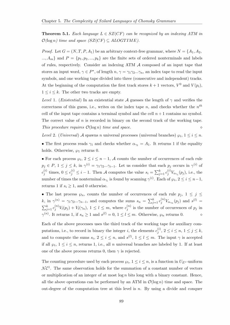
Chapter 5. The Complexity of Szilard Languages of Chomsky Grammars
Theorem 5.1. Each language L ∈ SZ(CF ) can be recognized by an indexing ATM in
O(log n) time and space (SZ(CF ) ⊆ ALOGTIME).
Proof. Let G = (N,T, P,A1) be an arbitrary context-free grammar, where N = A1, A2,
..., Am and P = p1, p2, ..., pk are the finite sets of ordered nonterminals and labels
of rules, respectively. Consider an indexing ATM A composed of an input tape that
stores an input word, γ ∈ P ∗, of length n, γ = γ1γ2...γn, an index tape to read the input
symbols, and one working tape divided into three (consecutive and independent) tracks.
At the beginning of the computation the first track stores k + 1 vectors, V 0 and V (pi),
1 ≤ i ≤ k. The other two tracks are empty.
Level 1. (Existential) In an existential state A guesses the length of γ and verifies the
correctness of this guess, i.e., writes on the index tape n, and checks whether the nth
cell of the input tape contains a terminal symbol and the cell n+ 1 contains no symbol.
The correct value of n is recorded in binary on the second track of the working tape.
This procedure requires O(log n) time and space.
Level 2. (Universal) A spawns n universal processes (universal branches) ℘i, 1 ≤ i ≤ n.
• The first process reads γ1 and checks whether αγ1 = A1. It returns 1 if the equality
holds. Otherwise, ℘1 returns 0.
• For each process ℘i, 2 ≤ i ≤ n − 1, A counts the number of occurrences of each rule
pj ∈ P , 1 ≤ j ≤ k, in γ(i) = γ1γ2...γi−1. Let us consider that each pj occurs in γ(i) of
c(i)j times, 0 ≤ c
(i)j ≤ i− 1. Then A computes the value si =
∑kj=1 c
(i)j Vαγi (pj), i.e., the
number of times the nonterminal αγi is found by scanning γ(i). Each of ℘i, 2 ≤ i ≤ n−1,
returns 1 if si ≥ 1, and 0 otherwise.
• The last process ℘n, counts the number of occurrences of each rule pj , 1 ≤ j ≤k, in γ(n) = γ1γ2...γn−1, and computes the sums sn =
∑kj=1 c
(n)j Vαγn (pj) and s(l) =∑k
j=1 c(n)j Vl(pj) + Vl(γn), 1 ≤ l ≤ m, where c
(n)j is the number of occurrences of pj in
γ(n). It returns 1, if sn ≥ 1 and s(l) = 0, 1 ≤ l ≤ m. Otherwise, ℘n returns 0.
Each of the above processes uses the third track of the working tape for auxiliary com-
putations, i.e., to record in binary the integer i, the elements c(i)j , 2 ≤ i ≤ n, 1 ≤ j ≤ k,
and to compute the sums si, 2 ≤ i ≤ n, and s(l), 1 ≤ l ≤ m. The input γ is accepted
if all ℘i, 1 ≤ i ≤ n, returns 1, i.e., all n universal branches are labeled by 1. If at least
one of the above process returns 0, then γ is rejected.
The counting procedure used by each process ℘i, 1 ≤ i ≤ n, is a function in UE∗-uniform
NC1. The same observation holds for the summation of a constant number of vectors
or multiplication of an integer of at most log n bits long with a binary constant. Hence,
all the above operations can be performed by an ATM in O(log n) time and space. The
out-degree of the computation tree at this level is n. By using a divide and conquer
89
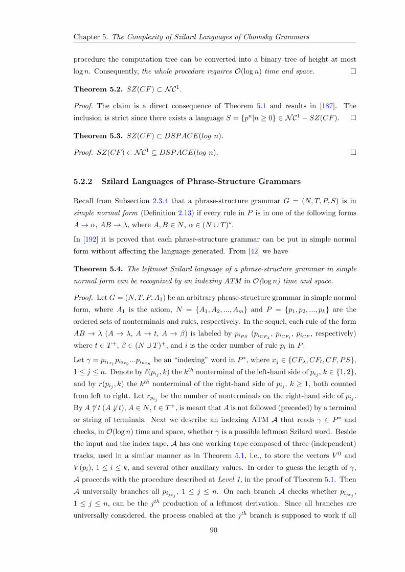
Chapter 5. The Complexity of Szilard Languages of Chomsky Grammars
procedure the computation tree can be converted into a binary tree of height at most
log n. Consequently, the whole procedure requires O(log n) time and space.
Theorem 5.2. SZ(CF ) ⊂ NC1.
Proof. The claim is a direct consequence of Theorem 5.1 and results in [187]. The
inclusion is strict since there exists a language S = pn|n ≥ 0 ∈ NC1 − SZ(CF ).
Theorem 5.3. SZ(CF ) ⊂ DSPACE(log n).
Proof. SZ(CF ) ⊂ NC1 ⊆ DSPACE(log n).
5.2.2 Szilard Languages of Phrase-Structure Grammars
Recall from Subsection 2.3.4 that a phrase-structure grammar G = (N,T, P, S) is in
simple normal form (Definition 2.13) if every rule in P is in one of the following forms
A→ α, AB → λ, where A,B ∈ N , α ∈ (N ∪ T )∗.
In [192] it is proved that each phrase-structure grammar can be put in simple normal
form without affecting the language generated. From [42] we have
Theorem 5.4. The leftmost Szilard language of a phrase-structure grammar in simple
normal form can be recognized by an indexing ATM in O(log n) time and space.
Proof. Let G = (N,T, P,A1) be an arbitrary phrase-structure grammar in simple normal
form, where A1 is the axiom, N = A1, A2, ..., Am and P = p1, p2, ..., pk are the
ordered sets of nonterminals and rules, respectively. In the sequel, each rule of the form
AB → λ (A → λ, A → t, A → β) is labeled by piPS (piCFλ , piCFt , piCF , respectively)
where t ∈ T+, β ∈ (N ∪ T )+, and i is the order number of rule pi in P .
Let γ = pi1x1pi2x2
...pinxn be an “indexing” word in P ∗, where xj ∈ CFλ, CFt, CF, PS,1 ≤ j ≤ n. Denote by `(pij , k) the kth nonterminal of the left-hand side of pij , k ∈ 1, 2,and by r(pij , k) the kth nonterminal of the right-hand side of pij , k ≥ 1, both counted
from left to right. Let rpij be the number of nonterminals on the right-hand side of pij .
By A 6↑ t (A 6↓ t), A ∈ N , t ∈ T+, is meant that A is not followed (preceded) by a terminal
or string of terminals. Next we describe an indexing ATM A that reads γ ∈ P ∗ and
checks, in O(log n) time and space, whether γ is a possible leftmost Szilard word. Beside
the input and the index tape, A has one working tape composed of three (independent)
tracks, used in a similar manner as in Theorem 5.1, i.e., to store the vectors V 0 and
V (pi), 1 ≤ i ≤ k, and several other auxiliary values. In order to guess the length of γ,
A proceeds with the procedure described at Level 1, in the proof of Theorem 5.1. Then
A universally branches all pijxj , 1 ≤ j ≤ n. On each branch A checks whether pijxj ,
1 ≤ j ≤ n, can be the jth production of a leftmost derivation. Since all branches are
universally considered, the process enabled at the jth branch is supposed to work if all
90
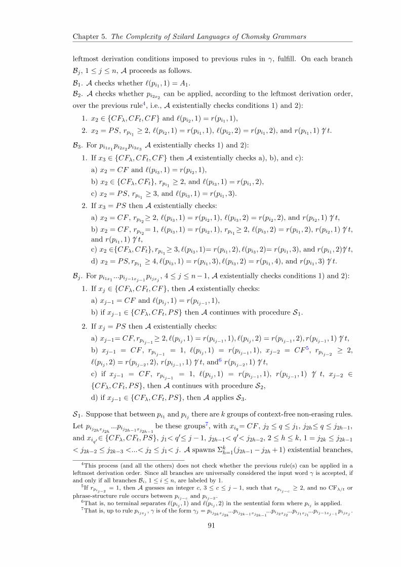
Chapter 5. The Complexity of Szilard Languages of Chomsky Grammars
leftmost derivation conditions imposed to previous rules in γ, fulfill. On each branch
Bj , 1 ≤ j ≤ n, A proceeds as follows.
B1. A checks whether `(pi1 , 1) = A1.
B2. A checks whether pi2x2can be applied, according to the leftmost derivation order,
over the previous rule4, i.e., A existentially checks conditions 1) and 2):
1. x2 ∈ CFλ, CFt, CF and `(pi2 , 1) = r(pi1 , 1),
2. x2 = PS, rpi1 ≥ 2, `(pi2 , 1) = r(pi1 , 1), `(pi2 , 2) = r(pi1 , 2), and r(pi1 , 1) 6↑ t.
B3. For pi1x1pi2x2
pi3x3A existentially checks 1) and 2):
1. If x3 ∈ CFλ, CFt, CF then A existentially checks a), b), and c):
a) x2 = CF and `(pi3 , 1) = r(pi2 , 1),
b) x2 ∈ CFλ, CFt, rpi1 ≥ 2, and `(pi3 , 1) = r(pi1 , 2),
c) x2 = PS, rpi1 ≥ 3, and `(pi3 , 1) = r(pi1 , 3).
2. If x3 = PS then A existentially checks:
a) x2 = CF , rpi2≥ 2, `(pi3 , 1) = r(pi2 , 1), `(pi3 , 2) = r(pi2 , 2), and r(pi2 , 1) 6↑ t,b) x2 = CF , rpi2 = 1, `(pi3 , 1) = r(pi2 , 1), rpi1≥ 2, `(pi3 , 2) = r(pi1 , 2), r(pi2 , 1) 6↑ t,and r(pi1 , 1) 6↑ t,c) x2 ∈CFλ, CFt, rpi1≥ 3, `(pi3 , 1)= r(pi1 , 2), `(pi3 , 2)= r(pi1 , 3), and r(pi1 , 2) 6↑ t,d) x2 = PS, rpi1 ≥ 4, `(pi3 , 1) = r(pi1 , 3), `(pi3 , 2) = r(pi1 , 4), and r(pi1 , 3) 6↑ t.
Bj . For pi1x1...pij−1xj−1
pijxj , 4 ≤ j ≤ n− 1, A existentially checks conditions 1) and 2):
1. If xj ∈ CFλ, CFt, CF, then A existentially checks:
a) xj−1 = CF and `(pij , 1) = r(pij−1 , 1),
b) if xj−1 ∈ CFλ, CFt, PS then A continues with procedure S1.
2. If xj = PS then A existentially checks:
a) xj−1= CF, rpij−1≥ 2, `(pij , 1) = r(pij−1 , 1), `(pij , 2) = r(pij−1 , 2), r(pij−1 , 1) 6↑ t,
b) xj−1 = CF , rpij−1= 1, `(pij , 1) = r(pij−1 , 1), xj−2 = CF 5, rpij−2
≥ 2,
`(pij , 2) = r(pij−2 , 2), r(pij−1 , 1) 6↑ t, and6 r(pij−2 , 1) 6↑ t,c) if xj−1 = CF , rpij−1
= 1, `(pij , 1) = r(pij−1 , 1), r(pij−1 , 1) 6↑ t, xj−2 ∈CFλ, CFt, PS, then A continues with procedure S2,
d) if xj−1 ∈ CFλ, CFt, PS, then A applies S3.
S1. Suppose that between pi1 and pij there are k groups of context-free non-erasing rules.
Let pij2hxj2h...pij2h−1xj2h−1
be these groups7, with xiq= CF , j2 ≤ q ≤ j1, j2h≤ q ≤ j2h−1,
and xiq′∈ CFλ, CFt, PS, j1< q′≤ j − 1, j2h−1< q′< j2h−2, 2 ≤ h ≤ k, 1 = j2k ≤ j2k−1
< j2k−2 ≤ j2k−3 <...< j2 ≤ j1< j. A spawns Σkh=1(j2h−1− j2h + 1) existential branches,
4This process (and all the others) does not check whether the previous rule(s) can be applied in aleftmost derivation order. Since all branches are universally considered the input word γ is accepted, ifand only if all branches Bi, 1 ≤ i ≤ n, are labeled by 1.
5If rpij−2= 1, then A guesses an integer c, 3 ≤ c ≤ j − 1, such that rpij−c ≥ 2, and no CFλ/t or
phrase-structure rule occurs between pij−c and pij−2 .6That is, no terminal separates `(pij , 1) and `(pij , 2) in the sentential form where pij is applied.7That is, up to rule pijxj , γ is of the form γj = pij2kxj2k
...pij2k−1xj2k−1...pij2xj2
...pij1xj1...pij−1xj−1
pijxj .
91
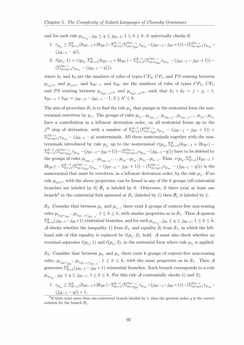
Chapter 5. The Complexity of Szilard Languages of Chomsky Grammars
and for each rule piqxiq, j2h ≤ q ≤ j2h−1, 1 ≤ h ≤ k, it universally checks if:
1. rpiq ≥ Σhh′=1(k2h′−1+2k2h′)−Σh−1
h′=1(Σj2h′−1
m=j2h′rpim−(j2h′−1−j2h′+1))−(Σ
j2h−1
m=q+1rpim−(j2h−1 − q)),
2. `(pij , 1) = r(piq ,Σhh′=1(k2h′−1 + 2k2h′)−Σh−1
h′=1(Σj2h′−1
m=j2h′rpim − (j2h′−1− j2h′ + 1))−
(Σj2h−1
m=q+1rpim − (j2h−1 − q))),
where k1 and k2 are the numbers of rules of types CFλ, CFt, and PS existing between
pij1CF and pijCF , and k2h′−1 and k2h′ are the numbers of rules of types CFλ, CFt,
and PS existing between pij2h′−1CFand pij2h′−2CF
, such that k1 + k2 = j − j1 − 1,
k2h′−1 + k2h′ = j2h′−2 − j2h′−1 − 1, 2 ≤ h′ ≤ k.
The aim of procedure S1 is to find the rule piq that pumps in the sentential form the non-
terminal rewritten by pij . The groups of rules piq ... pij2h−1, pij2h−2
...pij2h−3,..., pij2 ...pij1
have a contribution in a leftmost derivation order, on all sentential forms up to the
jth step of derivation, with a number of Σh−1h′=1(Σ
j2h′−1
m=j2h′rpim − (j2h′−1 − j2h′ + 1)) +
Σj2h−1
m=q+1rpim − (j2h−1 − q) nonterminals. All these nonterminals together with the non-
terminals introduced by rule piq up to the nonterminal r(piq ,Σhh′=1(k2h′−1 + 2k2h′) −
Σh−1h′=1(Σ
j2h′−1
m=j2h′rpim−(j2h′−1−j2h′+1))−(Σ
j2h−1
m=q+1rpim−(j2h−1−q))) have to be deleted by
the groups of rules pij2h−1...pij2h−2
, ..., pij2 ...pij1 , pij1 ...pij−1 . Thus, r(piq ,Σhh′=1(k2h′−1 +
2k2h′) − Σh−1h′=1(Σ
j2h′−1
m=j2h′rpim − (j2h′−1 − j2h′ + 1)) − (Σ
j2h−1
m=q+1rpim − (j2h−1 − q))) is the
nonterminal that must be rewritten, in a leftmost derivation order, by the rule pij . If no
rule piqCF , with the above properties, can be found in any of the k groups (all existential
branches are labeled by 0) Bj is labeled by 0. Otherwise, if there exist at least one
branch8 in the existential fork spawned at S1 (labeled by 1) then Bj is labeled by 1.
S2. Consider that between pi1 and pij−1 there exist k groups of context-free non-erasing
rules pij2hxj2h...pij2h−1xj2h−1
, 1 ≤ h ≤ k, with similar properties as in S1. Then A spawns
Σkh=1(j2h−1−j2h+1) existential branches, and for each piqxiq
, j2h ≤ q ≤ j2h−1, 1 ≤ h ≤ k,
A checks whether the inequality 1) from S1, and equality 2) from S1, in which the left-
hand side of this equality is replaced by `(pij , 2), hold. A must also check whether no
terminal separates `(pij , 1) and `(pij , 2), in the sentential form where rule pij is applied.
S3. Consider that between pi1 and pij there exist k groups of context-free non-erasing
rules, pij2hxj2h...pij2h−1xj2h−1
, 1 ≤ h ≤ k, with the same properties as in S1. Then Agenerates Σk
h=1(j2h−1− j2h + 1) existential branches. Each branch corresponds to a rule
piqxiq, j2h ≤ q ≤ j2h−1, 1 ≤ h ≤ k. For this rule A existentially checks 1) and 2):
1. rpiq ≥ Σhh′=1(k2h′−1+2k2h′)−Σh−1
h′=1(Σj2h′−1
m=j2h′rpim−(j2h′−1−j2h′+1))−(Σ
j2h−1
m=q+1rpim−(j2h−1 − q)) + 1,
8If there exist more than one existential branch labeled by 1, then the greatest index q is the correctsolution for the branch Bj .
92
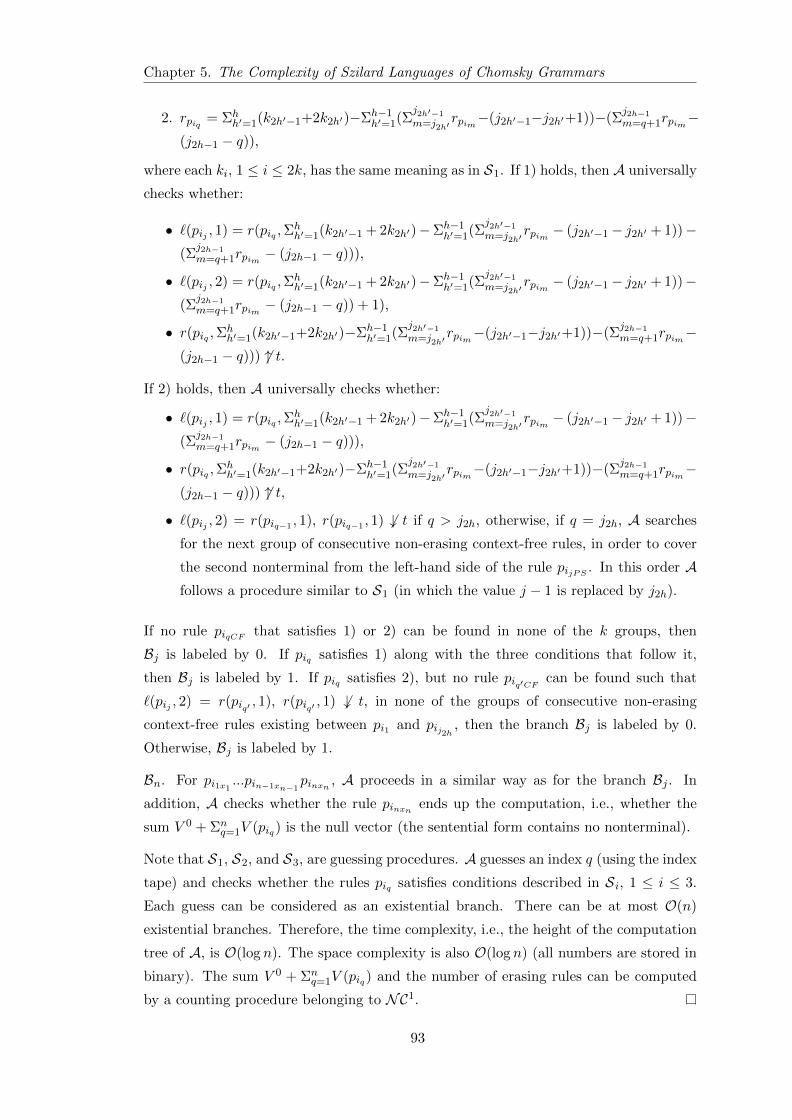
Chapter 5. The Complexity of Szilard Languages of Chomsky Grammars
2. rpiq = Σhh′=1(k2h′−1+2k2h′)−Σh−1
h′=1(Σj2h′−1
m=j2h′rpim−(j2h′−1−j2h′+1))−(Σ
j2h−1
m=q+1rpim−(j2h−1 − q)),
where each ki, 1 ≤ i ≤ 2k, has the same meaning as in S1. If 1) holds, then A universally
checks whether:
• `(pij , 1) = r(piq ,Σhh′=1(k2h′−1 + 2k2h′)−Σh−1
h′=1(Σj2h′−1
m=j2h′rpim − (j2h′−1− j2h′ + 1))−
(Σj2h−1
m=q+1rpim − (j2h−1 − q))),
• `(pij , 2) = r(piq ,Σhh′=1(k2h′−1 + 2k2h′)−Σh−1
h′=1(Σj2h′−1
m=j2h′rpim − (j2h′−1− j2h′ + 1))−
(Σj2h−1
m=q+1rpim − (j2h−1 − q)) + 1),
• r(piq ,Σhh′=1(k2h′−1+2k2h′)−Σh−1
h′=1(Σj2h′−1
m=j2h′rpim−(j2h′−1−j2h′+1))−(Σ
j2h−1
m=q+1rpim−(j2h−1 − q))) 6↑ t.
If 2) holds, then A universally checks whether:
• `(pij , 1) = r(piq ,Σhh′=1(k2h′−1 + 2k2h′)−Σh−1
h′=1(Σj2h′−1
m=j2h′rpim − (j2h′−1− j2h′ + 1))−
(Σj2h−1
m=q+1rpim − (j2h−1 − q))),
• r(piq ,Σhh′=1(k2h′−1+2k2h′)−Σh−1
h′=1(Σj2h′−1
m=j2h′rpim−(j2h′−1−j2h′+1))−(Σ
j2h−1
m=q+1rpim−(j2h−1 − q))) 6↑ t,
• `(pij , 2) = r(piq−1 , 1), r(piq−1 , 1) 6↓ t if q > j2h, otherwise, if q = j2h, A searches
for the next group of consecutive non-erasing context-free rules, in order to cover
the second nonterminal from the left-hand side of the rule pijPS . In this order Afollows a procedure similar to S1 (in which the value j − 1 is replaced by j2h).
If no rule piqCF that satisfies 1) or 2) can be found in none of the k groups, then
Bj is labeled by 0. If piq satisfies 1) along with the three conditions that follow it,
then Bj is labeled by 1. If piq satisfies 2), but no rule piq′CF can be found such that
`(pij , 2) = r(piq′ , 1), r(piq′ , 1) 6↓ t, in none of the groups of consecutive non-erasing
context-free rules existing between pi1 and pij2h , then the branch Bj is labeled by 0.
Otherwise, Bj is labeled by 1.
Bn. For pi1x1...pin−1xn−1
pinxn , A proceeds in a similar way as for the branch Bj . In
addition, A checks whether the rule pinxn ends up the computation, i.e., whether the
sum V 0 + Σnq=1V (piq) is the null vector (the sentential form contains no nonterminal).
Note that S1, S2, and S3, are guessing procedures. A guesses an index q (using the index
tape) and checks whether the rules piq satisfies conditions described in Si, 1 ≤ i ≤ 3.
Each guess can be considered as an existential branch. There can be at most O(n)
existential branches. Therefore, the time complexity, i.e., the height of the computation
tree of A, is O(log n). The space complexity is also O(log n) (all numbers are stored in
binary). The sum V 0 + Σnq=1V (piq) and the number of erasing rules can be computed
by a counting procedure belonging to NC1.
93
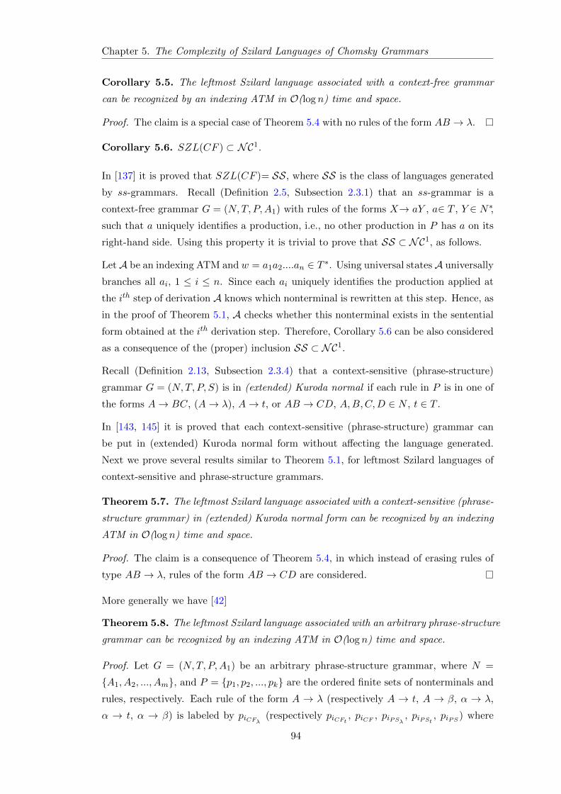
Chapter 5. The Complexity of Szilard Languages of Chomsky Grammars
Corollary 5.5. The leftmost Szilard language associated with a context-free grammar
can be recognized by an indexing ATM in O(log n) time and space.
Proof. The claim is a special case of Theorem 5.4 with no rules of the form AB → λ.
Corollary 5.6. SZL(CF ) ⊂ NC1.
In [137] it is proved that SZL(CF )= SS, where SS is the class of languages generated
by ss-grammars. Recall (Definition 2.5, Subsection 2.3.1) that an ss-grammar is a
context-free grammar G = (N,T, P,A1) with rules of the forms X→ aY , a∈ T , Y ∈ N∗,such that a uniquely identifies a production, i.e., no other production in P has a on its
right-hand side. Using this property it is trivial to prove that SS ⊂ NC1, as follows.
LetA be an indexing ATM and w = a1a2....an ∈ T ∗. Using universal statesA universally
branches all ai, 1 ≤ i ≤ n. Since each ai uniquely identifies the production applied at
the ith step of derivation A knows which nonterminal is rewritten at this step. Hence, as
in the proof of Theorem 5.1, A checks whether this nonterminal exists in the sentential
form obtained at the ith derivation step. Therefore, Corollary 5.6 can be also considered
as a consequence of the (proper) inclusion SS ⊂ NC1.
Recall (Definition 2.13, Subsection 2.3.4) that a context-sensitive (phrase-structure)
grammar G = (N,T, P, S) is in (extended) Kuroda normal if each rule in P is in one of
the forms A→ BC, (A→ λ), A→ t, or AB → CD, A,B,C,D ∈ N , t ∈ T .
In [143, 145] it is proved that each context-sensitive (phrase-structure) grammar can
be put in (extended) Kuroda normal form without affecting the language generated.
Next we prove several results similar to Theorem 5.1, for leftmost Szilard languages of
context-sensitive and phrase-structure grammars.
Theorem 5.7. The leftmost Szilard language associated with a context-sensitive (phrase-
structure grammar) in (extended) Kuroda normal form can be recognized by an indexing
ATM in O(log n) time and space.
Proof. The claim is a consequence of Theorem 5.4, in which instead of erasing rules of
type AB → λ, rules of the form AB → CD are considered.
More generally we have [42]
Theorem 5.8. The leftmost Szilard language associated with an arbitrary phrase-structure
grammar can be recognized by an indexing ATM in O(log n) time and space.
Proof. Let G = (N,T, P,A1) be an arbitrary phrase-structure grammar, where N =
A1, A2, ..., Am, and P = p1, p2, ..., pk are the ordered finite sets of nonterminals and
rules, respectively. Each rule of the form A → λ (respectively A → t, A → β, α → λ,
α → t, α → β) is labeled by piCFλ (respectively piCFt , piCF , piPSλ , piPSt , piPS ) where
94
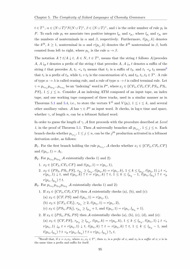
Chapter 5. The Complexity of Szilard Languages of Chomsky Grammars
t ∈ T+, α ∈ (N ∪ T )∗N(N ∪ T )∗, β ∈ (N ∪ T )+, and i is the order number of rule pi in
P . To each rule pi we associate two positive integers lpi and rpi , where lpi and rpi are
the numbers of nonterminals in α and β, respectively. Furthermore, `(pij , k) denotes
the kth, k ≥ 1, nonterminal in α and r(pij , k) denotes the kth nonterminal in β, both
counted from left to right, where pij is the rule α→ β.
The notation A ↑ t/A ↓ t, A ∈ N , t ∈ T ∗, means that the string t follows A/precedes
A, A ↓p t denotes a prefix of the string t that precedes A, A ↓s t denotes a suffix of the
string t that precedes A, t1 ≺s t2 means that t1 is a suffix of t2, and t1 ≺p t2 means9
that t1 is a prefix of t2, while t1 + t2 is the concatenation of t1 and t2, t1, t2 ∈ T ∗. A rule
of type α→ λ is called erasing rule, and a rule of type α→ t is called terminal rule. Let
γ = pi1x1pi2x2
...pinxn be an “indexing” word in P ∗, where xj ∈ CFλ, CFt, CF, PSλ, PSt,PS, 1 ≤ j ≤ n. Consider A an indexing ATM composed of an input tape, an index
tape, and one working tape composed of three tracks, used in a similar manner as in
Theorems 5.1 and 5.4, i.e., to store the vectors V 0 and V (pi), 1 ≤ i ≤ k, and several
other auxiliary values. A has γ ∈ P ∗ as input word. It checks, in log n time and space,
whether γ, of length n, can be a leftmost Szilard word.
In order to guess the length of γ, A first proceeds with the procedure described at Level
1, in the proof of Theorem 5.1. Then A universally branches all pijxj , 1 ≤ j ≤ n. Each
branch checks whether pijxj , 1 ≤ j ≤ n, can be the jth production activated in a leftmost
derivation order, as follows:
B1. For the first branch holding the rule pi1x1, A checks whether x1 ∈ CFλ, CFt, CF
and `(pi1 , 1) = A1.
B2. For pi1x1pi2x2
A existentially checks 1) and 2):
1. x2 ∈ CFλ, CFt, CF and `(pi2 , 1) = r(pi1 , 1),
2. x2 ∈ PSλ, PSt, PS, rpi1 ≥ lpi2 , `(pi2 , k) = r(pi1 , k), 1 ≤ k ≤ lpi2 , `(pi2 , 1) ↓ t ≺sr(pi1 , 1) ↓ t, and `(pi2 , k) ↑ t = r(pi1 , k) ↑ t, 1 ≤ k ≤ lpi2 − 1, `(pi2 , lpi2 ) ↑ t ≺pr(pi1 , lpi2 ) ↑ t.
B3. For pi1x1pi2x2
pi3x3A existentially checks 1) and 2):
1. If x3 ∈ CFλ, CFt, CF then A existentially checks (a), (b), and (c):
(a) x2 ∈ CF,PS and `(pi3 , 1) = r(pi2 , 1),
(b) x2 ∈ CFλ, CFt, rpi1 ≥ 2, `(pi3 , 1) = r(pi1 , 2),
(c) x2 ∈ PSλ, PSt, rpi1 ≥ lpi2 + 1, and `(pi3 , 1) = r(pi1 , lpi2 + 1).
2. If x3 ∈ PSλ, PSt, PS then A existentially checks (a), (b), (c), (d), and (e):
(a) x2 ∈ CF,PS, rpi2 ≥ lpi3 , `(pi3 , k) = r(pi2 , k), 1 ≤ k ≤ lpi3 , `(pi3 , 1) ↓ t ≺sr(pi1 , 1) ↓p t + r(pi2 , 1) ↓ t, `(pi3 , k) ↑ t = r(pi2 , k) ↑ t, 1 ≤ k ≤ lpi3 − 1, and
`(pi3 , lpi3 ) ↑ t ≺p r(pi2 , lpi3 ) ↑ t+ r(pi1 , lpi2 ) ↑s t,9Recall that, if x = x1x2, where x1, x2 ∈ T ∗, then x1 is a prefix of x, and x2 is a suffix of x; x is in
the same time a prefix and suffix for itself.
95
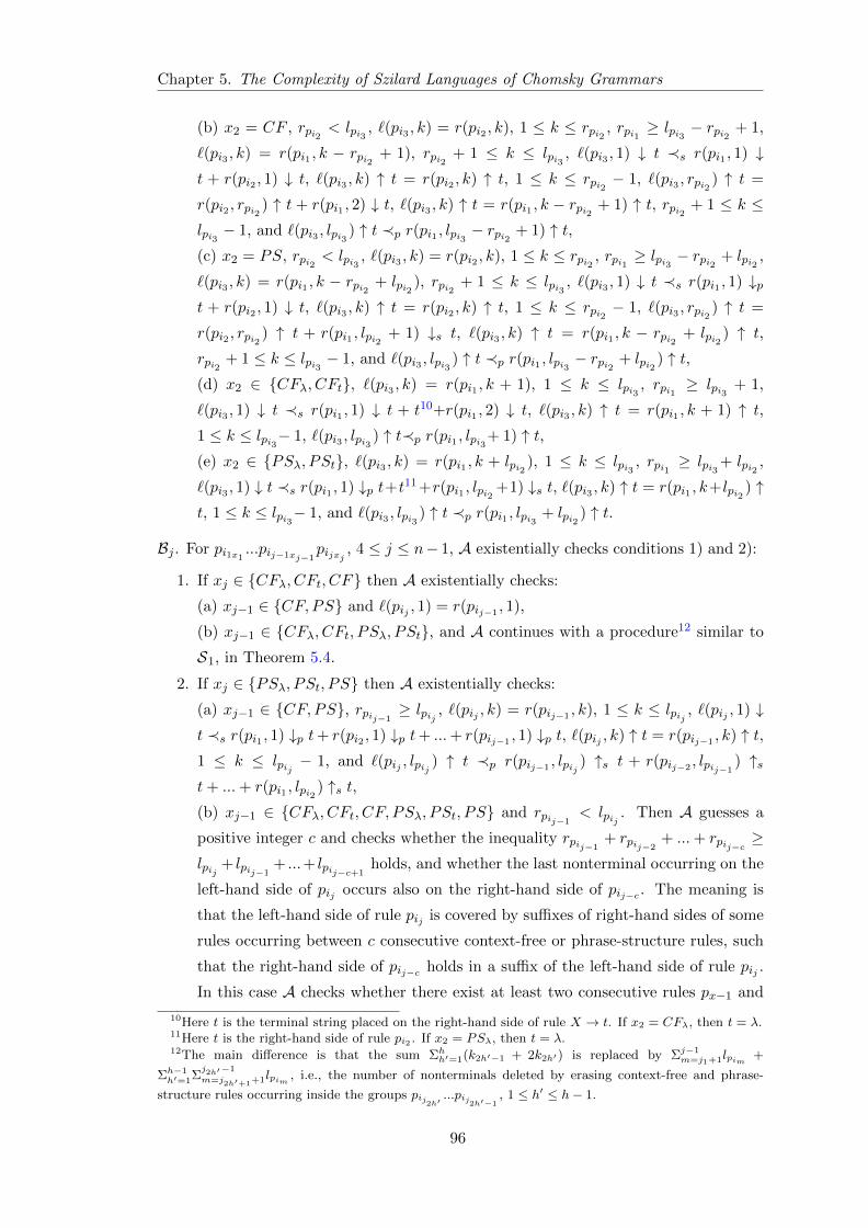
Chapter 5. The Complexity of Szilard Languages of Chomsky Grammars
(b) x2 = CF , rpi2 < lpi3 , `(pi3 , k) = r(pi2 , k), 1 ≤ k ≤ rpi2 , rpi1 ≥ lpi3 − rpi2 + 1,
`(pi3 , k) = r(pi1 , k − rpi2 + 1), rpi2 + 1 ≤ k ≤ lpi3 , `(pi3 , 1) ↓ t ≺s r(pi1 , 1) ↓t + r(pi2 , 1) ↓ t, `(pi3 , k) ↑ t = r(pi2 , k) ↑ t, 1 ≤ k ≤ rpi2 − 1, `(pi3 , rpi2 ) ↑ t =
r(pi2 , rpi2 ) ↑ t + r(pi1 , 2) ↓ t, `(pi3 , k) ↑ t = r(pi1 , k − rpi2 + 1) ↑ t, rpi2 + 1 ≤ k ≤lpi3 − 1, and `(pi3 , lpi3 ) ↑ t ≺p r(pi1 , lpi3 − rpi2 + 1) ↑ t,(c) x2 = PS, rpi2 < lpi3 , `(pi3 , k) = r(pi2 , k), 1 ≤ k ≤ rpi2 , rpi1 ≥ lpi3 − rpi2 + lpi2 ,
`(pi3 , k) = r(pi1 , k − rpi2 + lpi2 ), rpi2 + 1 ≤ k ≤ lpi3 , `(pi3 , 1) ↓ t ≺s r(pi1 , 1) ↓pt + r(pi2 , 1) ↓ t, `(pi3 , k) ↑ t = r(pi2 , k) ↑ t, 1 ≤ k ≤ rpi2 − 1, `(pi3 , rpi2 ) ↑ t =
r(pi2 , rpi2 ) ↑ t + r(pi1 , lpi2 + 1) ↓s t, `(pi3 , k) ↑ t = r(pi1 , k − rpi2 + lpi2 ) ↑ t,rpi2 + 1 ≤ k ≤ lpi3 − 1, and `(pi3 , lpi3 ) ↑ t ≺p r(pi1 , lpi3 − rpi2 + lpi2 ) ↑ t,(d) x2 ∈ CFλ, CFt, `(pi3 , k) = r(pi1 , k + 1), 1 ≤ k ≤ lpi3 , rpi1 ≥ lpi3 + 1,
`(pi3 , 1) ↓ t ≺s r(pi1 , 1) ↓ t + t10+r(pi1 , 2) ↓ t, `(pi3 , k) ↑ t = r(pi1 , k + 1) ↑ t,1 ≤ k ≤ lpi3− 1, `(pi3 , lpi3 ) ↑ t≺p r(pi1 , lpi3+ 1) ↑ t,(e) x2 ∈ PSλ, PSt, `(pi3 , k) = r(pi1 , k + lpi2 ), 1 ≤ k ≤ lpi3 , rpi1 ≥ lpi3 + lpi2 ,
`(pi3 , 1) ↓ t ≺s r(pi1 , 1) ↓p t+t11 +r(pi1 , lpi2 +1) ↓s t, `(pi3 , k) ↑ t = r(pi1 , k+lpi2 ) ↑t, 1 ≤ k ≤ lpi3− 1, and `(pi3 , lpi3 ) ↑ t ≺p r(pi1 , lpi3 + lpi2 ) ↑ t.
Bj . For pi1x1...pij−1xj−1
pijxj , 4 ≤ j ≤ n− 1, A existentially checks conditions 1) and 2):
1. If xj ∈ CFλ, CFt, CF then A existentially checks:
(a) xj−1 ∈ CF,PS and `(pij , 1) = r(pij−1 , 1),
(b) xj−1 ∈ CFλ, CFt, PSλ, PSt, and A continues with a procedure12 similar to
S1, in Theorem 5.4.
2. If xj ∈ PSλ, PSt, PS then A existentially checks:
(a) xj−1 ∈ CF,PS, rpij−1≥ lpij , `(pij , k) = r(pij−1 , k), 1 ≤ k ≤ lpij , `(pij , 1) ↓
t ≺s r(pi1 , 1) ↓p t+ r(pi2 , 1) ↓p t+ ...+ r(pij−1 , 1) ↓p t, `(pij , k) ↑ t = r(pij−1 , k) ↑ t,1 ≤ k ≤ lpij − 1, and `(pij , lpij ) ↑ t ≺p r(pij−1 , lpij ) ↑s t + r(pij−2 , lpij−1
) ↑st+ ...+ r(pi1 , lpi2 ) ↑s t,(b) xj−1 ∈ CFλ, CFt, CF, PSλ, PSt, PS and rpij−1
< lpij . Then A guesses a
positive integer c and checks whether the inequality rpij−1+ rpij−2
+ ...+ rpij−c ≥lpij + lpij−1
+ ...+ lpij−c+1holds, and whether the last nonterminal occurring on the
left-hand side of pij occurs also on the right-hand side of pij−c . The meaning is
that the left-hand side of rule pij is covered by suffixes of right-hand sides of some
rules occurring between c consecutive context-free or phrase-structure rules, such
that the right-hand side of pij−c holds in a suffix of the left-hand side of rule pij .
In this case A checks whether there exist at least two consecutive rules px−1 and
10Here t is the terminal string placed on the right-hand side of rule X → t. If x2 = CFλ, then t = λ.11Here t is the right-hand side of rule pi2 . If x2 = PSλ, then t = λ.12The main difference is that the sum Σhh′=1(k2h′−1 + 2k2h′) is replaced by Σj−1
m=j1+1lpim +
Σh−1h′=1Σ
j2h′−1
m=j2h′+1+1lpim , i.e., the number of nonterminals deleted by erasing context-free and phrase-
structure rules occurring inside the groups pij2h′...pij
2h′−1, 1 ≤ h′ ≤ h− 1.
96
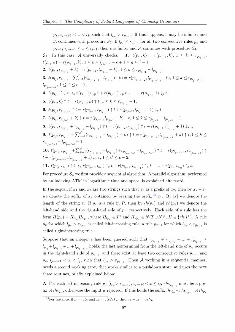
Chapter 5. The Complexity of Szilard Languages of Chomsky Grammars
px, ij−c+1 < x < ij , such that lpx > rpx−1 . If this happens, c may be infinite, and
A continues with procedure S5. If lpx ≤ rpx−1 for all two consecutive rules px and
px−1, ij−c+1 ≤ x ≤ ij−1, then c is finite, and A continues with procedure S4.
S4. In this case, A universally checks: 1. `(pij , k) = r(pij−1 , k), 1 ≤ k ≤ rpij−1,
`(piq , k) = r(piq−1 , k), 1 ≤ k ≤ lpiq , j − c+ 1 ≤ q ≤ j − 1,
2. `(pij , rpij−1+ k) = r(pij−2 , lpij−1
+ k), 1 ≤ k ≤ rpij−2− lpij−1
,
3. `(pij , rpij−1+∑c′
x=1(rpij−x−1−lpij−x )+k) = r(pij−c′−2
, lpij−c′−1+k), 1 ≤ k ≤ rpij−c′−2
−lpij−c′−1
, 1 ≤ c′ ≤ c− 2,
4. `(pij , 1) ↓ t ≺s r(pi1 , 1) ↓p t+ r(pi2 , 1) ↓p t+ ...+ r(pij−1 , 1) ↓p t,
5. `(pij , k) ↑ t = r(pij−1 , k) ↑ t, 1 ≤ k ≤ rpij−1− 1,
6. `(pij , rpij−1) ↑ t = r(pij−1 , rpij−1
) ↑ t+ r(pij−2 , lpij−1+ 1) ↓s t,
7. `(pij , rpij−1+ k) ↑ t = r(pij−2 , lpij−1
+ k) ↑ t, 1 ≤ k ≤ rpij−2− lpij−1
− 1
8. `(pij , rpij−1+ rpij−2
− lpij−1) ↑ t = r(pij−2 , rpij−2
) ↑ t+ r(pij−3 , lpij−2+ 1) ↓s t,
9. `(pij , rpij−1+∑c′
x=1(rpij−x−1− lpij−x ) + k) ↑ t = r(pij−c′−2
, lpij−c′−1+ k) ↑ t, 1 ≤ k ≤
rpij−c′−2− lpij−c′−1
− 1,
10. `(pij , rpij−1+∑c′
x=1(rpij−x−1−lpij−x )+rpij−c′−2
−lpij−c′−1) ↑ t = r(pij−c′−2
, rpij−c′−2) ↑
t+ r(pij−c′−3, lpij−c′−2
+ 1) ↓s t, 1 ≤ c′ ≤ c− 2,
11. `(pij , lpij ) ↑ t ≺p r(pij−1 , lpij ) ↑s t+ r(pij−2 , lpij−1) ↑s t+ ...+ r(pi1 , lpi2 ) ↑s t.
For procedure S5 we first provide a sequential algorithm. A parallel algorithm, performed
by an indexing ATM in logarithmic time and space, is explained afterward.
In the sequel, if x1 and x2 are two strings such that x1 is a prefix of x2, then by x2− x1
we denote the suffix of x2 obtained by erasing the prefix13 x1. By |x| we denote the
length of the string x. If px is a rule in P , then by lh(px) and rh(px) we denote the
left-hand side and the right-hand side of px, respectively. Each side of a rule has the
form H(px) = HtpxHVpx , where Htpx ∈ T∗ and HVpx ∈ N(T ∪N)∗, H ∈ rh, lh. A rule
px for which lpx > rpx−1 is called left-increasing rule, a rule px−1 for which lpx < rpx−1 is
called right-increasing rule.
Suppose that an integer c has been guessed such that rpij−1+ rpij−2
+ ... + rpij−c ≥lpij + lpij−1
+ ...+ lpij−c+1holds, the last nonterminal from the left-hand side of pij occurs
in the right-hand side of pij−c , and there exist at least two consecutive rules px−1 and
px, ij−c+1 < x < ij , such that lpx > rpx−1 . Then A working in a sequential manner,
needs a second working tape, that works similar to a pushdown store, and uses the next
three routines, briefly explained below.
A. For each left-increasing rule px (lpx> rpx−1), ij−c+1< x ≤ ij , rhVpx−1must be a pre-
fix of lhVpx , otherwise the input is rejected. If this holds the suffix lhVpx−rhVpx−1of lhpx
13For instance, if x1 = abc and x2 = abcdefg, then x2 − x1 = defg.
97
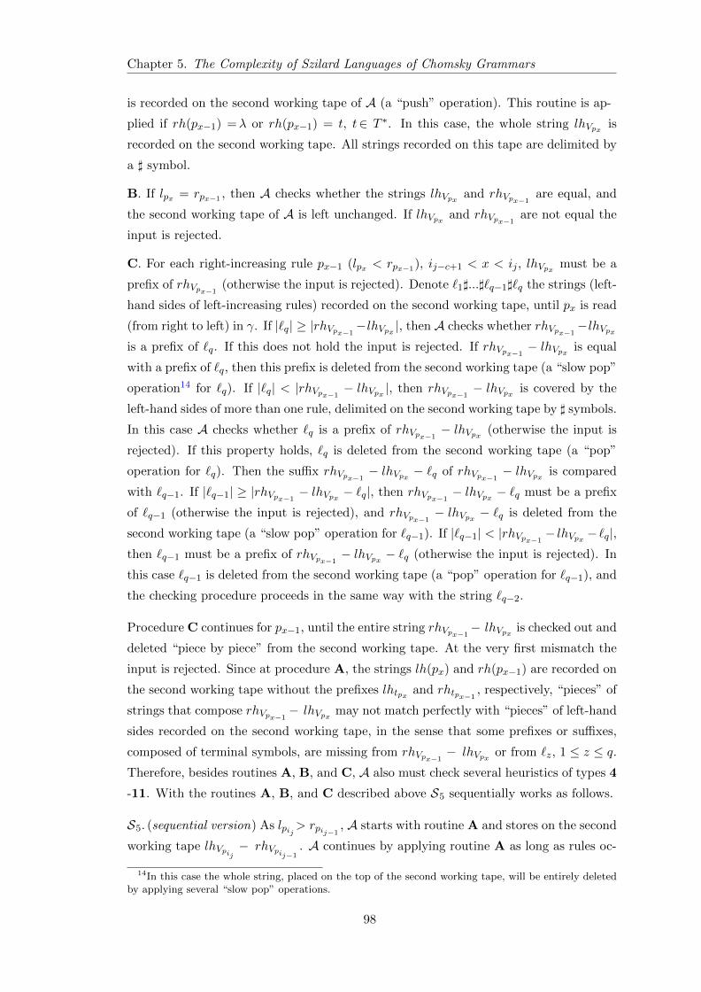
Chapter 5. The Complexity of Szilard Languages of Chomsky Grammars
is recorded on the second working tape of A (a “push” operation). This routine is ap-
plied if rh(px−1) =λ or rh(px−1) = t, t∈ T ∗. In this case, the whole string lhVpx is
recorded on the second working tape. All strings recorded on this tape are delimited by
a ] symbol.
B. If lpx = rpx−1 , then A checks whether the strings lhVpx and rhVpx−1are equal, and
the second working tape of A is left unchanged. If lhVpx and rhVpx−1are not equal the
input is rejected.
C. For each right-increasing rule px−1 (lpx < rpx−1), ij−c+1 < x < ij , lhVpx must be a
prefix of rhVpx−1(otherwise the input is rejected). Denote `1]...]`q−1]`q the strings (left-
hand sides of left-increasing rules) recorded on the second working tape, until px is read
(from right to left) in γ. If |`q| ≥ |rhVpx−1−lhVpx |, then A checks whether rhVpx−1
−lhVpxis a prefix of `q. If this does not hold the input is rejected. If rhVpx−1
− lhVpx is equal
with a prefix of `q, then this prefix is deleted from the second working tape (a “slow pop”
operation14 for `q). If |`q| < |rhVpx−1− lhVpx |, then rhVpx−1
− lhVpx is covered by the
left-hand sides of more than one rule, delimited on the second working tape by ] symbols.
In this case A checks whether `q is a prefix of rhVpx−1− lhVpx (otherwise the input is
rejected). If this property holds, `q is deleted from the second working tape (a “pop”
operation for `q). Then the suffix rhVpx−1− lhVpx − `q of rhVpx−1
− lhVpx is compared
with `q−1. If |`q−1| ≥ |rhVpx−1− lhVpx − `q|, then rhVpx−1
− lhVpx − `q must be a prefix
of `q−1 (otherwise the input is rejected), and rhVpx−1− lhVpx − `q is deleted from the
second working tape (a “slow pop” operation for `q−1). If |`q−1| < |rhVpx−1− lhVpx − `q|,
then `q−1 must be a prefix of rhVpx−1− lhVpx − `q (otherwise the input is rejected). In
this case `q−1 is deleted from the second working tape (a “pop” operation for `q−1), and
the checking procedure proceeds in the same way with the string `q−2.
Procedure C continues for px−1, until the entire string rhVpx−1− lhVpx is checked out and
deleted “piece by piece” from the second working tape. At the very first mismatch the
input is rejected. Since at procedure A, the strings lh(px) and rh(px−1) are recorded on
the second working tape without the prefixes lhtpx and rhtpx−1, respectively, “pieces” of
strings that compose rhVpx−1− lhVpx may not match perfectly with “pieces” of left-hand
sides recorded on the second working tape, in the sense that some prefixes or suffixes,
composed of terminal symbols, are missing from rhVpx−1− lhVpx or from `z, 1 ≤ z ≤ q.
Therefore, besides routines A, B, and C, A also must check several heuristics of types 4
-11. With the routines A, B, and C described above S5 sequentially works as follows.
S5. (sequential version) As lpij> rpij−1, A starts with routine A and stores on the second
working tape lhVpij− rhVpij−1
. A continues by applying routine A as long as rules oc-
14In this case the whole string, placed on the top of the second working tape, will be entirely deletedby applying several “slow pop” operations.
98
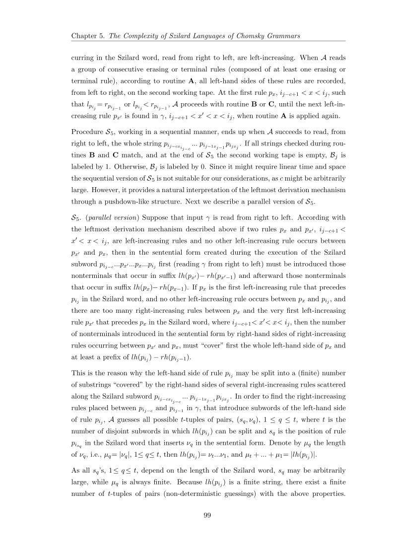
Chapter 5. The Complexity of Szilard Languages of Chomsky Grammars
curring in the Szilard word, read from right to left, are left-increasing. When A reads
a group of consecutive erasing or terminal rules (composed of at least one erasing or
terminal rule), according to routine A, all left-hand sides of these rules are recorded,
from left to right, on the second working tape. At the first rule px, ij−c+1 < x < ij , such
that lpij = rpij−1or lpij< rpij−1
, A proceeds with routine B or C, until the next left-in-
creasing rule px′ is found in γ, ij−c+1 < x′ < x < ij , when routine A is applied again.
Procedure S5, working in a sequential manner, ends up when A succeeds to read, from
right to left, the whole string pij−cxij−c... pij−1xj−1
pijxj . If all strings checked during rou-
tines B and C match, and at the end of S5 the second working tape is empty, Bj is
labeled by 1. Otherwise, Bj is labeled by 0. Since it might require linear time and space
the sequential version of S5 is not suitable for our considerations, as cmight be arbitrarily
large. However, it provides a natural interpretation of the leftmost derivation mechanism
through a pushdown-like structure. Next we describe a parallel version of S5.
S5. (parallel version) Suppose that input γ is read from right to left. According with
the leftmost derivation mechanism described above if two rules px and px′ , ij−c+1 <
x′ < x< ij , are left-increasing rules and no other left-increasing rule occurs between
px′ and px, then in the sentential form created during the execution of the Szilard
subword pij−c ...px′ ...px...pij first (reading γ from right to left) must be introduced those
nonterminals that occur in suffix lh(px′)− rh(px′−1) and afterward those nonterminals
that occur in suffix lh(px)− rh(px−1). If px is the first left-increasing rule that precedes
pij in the Szilard word, and no other left-increasing rule occurs between px and pij , and
there are too many right-increasing rules between px and the very first left-increasing
rule px′ that precedes px in the Szilard word, where ij−c+1< x′< x< ij , then the number
of nonterminals introduced in the sentential form by right-hand sides of right-increasing
rules occurring between px′ and px, must “cover” first the whole left-hand side of px and
at least a prefix of lh(pij )− rh(pij−1).
This is the reason why the left-hand side of rule pij may be split into a (finite) number
of substrings “covered” by the right-hand sides of several right-increasing rules scattered
along the Szilard subword pij−cxij−c... pij−1xj−1
pijxj . In order to find the right-increasing
rules placed between pij−c and pij−1 in γ, that introduce subwords of the left-hand side
of rule pij , A guesses all possible t-tuples of pairs, (sq, νq), 1 ≤ q ≤ t, where t is the
number of disjoint subwords in which lh(pij ) can be split and sq is the position of rule
pisq in the Szilard word that inserts νq in the sentential form. Denote by µq the length
of νq, i.e., µq= |νq|, 1≤ q≤ t, then lh(pij )= νt...ν1, and µt + ...+ µ1= |lh(pij )|.
As all sq’s, 1≤ q≤ t, depend on the length of the Szilard word, sq may be arbitrarily
large, while µq is always finite. Because lh(pij ) is a finite string, there exist a finite
number of t-tuples of pairs (non-deterministic guessings) with the above properties.
99
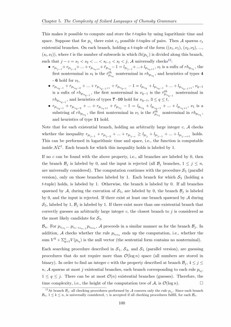
Chapter 5. The Complexity of Szilard Languages of Chomsky Grammars
This makes it possible to compute and store the t-tuples by using logarithmic time and
space. Suppose that for pij there exist cs possible t-tuples of pairs. Then A spawns cs
existential branches. On each branch, holding a t-tuple of the form ((s1, ν1), (s2, ν2), ...,
(st, νt)), where t is the number of subwords in which lh(pij ) is divided along this branch,
such that j − c = s1 < s2 < ... < st−1 < st < j, A universally checks15:
• rpij−1+ rpij−2
+ ...+ rpist+1+ rpist
− 1 = lpij−1+ ...+ lpist+1
, νt is a sufix of rhpist, the
first nonterminal in νt is the rthpistnonterminal in rhpist
, and heuristics of types 4
- 6 hold for νt,• rpisq−1
+ rpisq−2+ ...+ rpisq−1+1
+ rpisq−1− 1 = lpisq + lpisq−1
+ ...+ lpisq−1+1, νq−1
is a sufix of rhpisq−1, the first nonterminal in νq−1 is the rthpisq−1
nonterminal in
rhpisq−1, and heuristics of types 7 -10 hold for νq−1, 3 ≤ q ≤ t,
• rpis2−1+ rpis2−2
+ ... + rpis1+1+ rpis1
− 1 = lpis2+ lpis2−1
+ ... + lpis1+1, ν1 is a
substring of rhpis1, the first nonterminal in ν1 is the rthpis1
nonterminal in rhpis1,
and heuristics of type 11 hold.
Note that for each existential branch, holding an arbitrarily large integer c, A checks
whether the inequality rpij−1+ rpij−2
+ ... + rpij−c ≥ lpij + lpij−1+ ... + lpij−c+1
holds.
This can be performed in logarithmic time and space, i.e., the function is computable
inside NC1. Each branch for which this inequality holds is labeled by 1.
If no c can be found with the above property, i.e., all branches are labeled by 0, then
the branch Bj is labeled by 0, and the input is rejected (all Bj branches, 1 ≤ j ≤ n,
are universally considered). The computation continues with the procedure S5 (parallel
version), only on those branches labeled by 1. Each branch for which S5 (holding a
t-tuple) holds, is labeled by 1. Otherwise, the branch is labeled by 0. If all branches
spawned by A, during the execution of S5, are labeled by 0, the branch Bj is labeled
by 0, and the input is rejected. If there exist at least one branch spawned by A during
S5, labeled by 1, Bj is labeled by 1. If there exist more than one existential branch that
correctly guesses an arbitrarily large integer c, the closest branch to j is considered as
the most likely candidate for S5.
Bn. For pi1x1... pin−1xn−1
pinxn , A proceeds in a similar manner as for the branch Bj . In
addition, A checks whether the rule pinxn ends up the computation, i.e., whether the
sum V 0 + Σnq=1V (piq) is the null vector (the sentential form contains no nonterminal).
Each searching procedure described in S1, S4, and S5 (parallel version), are guessing
procedures that do not require more than O(log n) space (all numbers are stored in
binary). In order to find an integer c with the property described at branch Bj , 4 ≤ j ≤n, A spawns at most j existential branches, each branch corresponding to each rule piq ,
1 ≤ q ≤ j. There can be at most O(n) existential branches (guesses). Therefore, the
time complexity, i.e., the height of the computation tree of A, is O(log n).
15At branch Bj , all checking procedures performed by A concern only the rule pij . Since each branchBk, 1 ≤ k ≤ n, is universally considered, γ is accepted if all checking procedures fulfill, for each Bk.
100
Chapter 5. The Complexity of Szilard Languages of Chomsky Grammars
Theorem 5.9. SZL(PS) ⊂ NC1.
Proof. The claim is a direct consequence of Theorem 5.8 and results in [187]. The
inclusion is strict, since the language S = pn|n ≥ 0 belongs to NC1 − SZL(PS).
Theorem 5.10. SZL(PS) ⊂ DSPACE(log n).
Proof. SZL(PS) ⊂ NC1 ⊆ DSPACE(log n).
Corollary 5.11. Leftmost Szilard languages of context-sensitive grammars can be rec-
ognized by indexing ATMs in O(log n) time and space.
Proof. The result is a consequence of Theorem 5.8, in which all phrase-structure rules
are length-increasing, i.e., α→ β, |α| ≤ |β|, and no erasing rule is allowed.
Corollary 5.12. SZL(CS) ⊂ NC1 ⊆ DSPACE(log n).
5.3 Conclusions and Further Investigations
In this chapter we have investigated computational resources, such as time and space,
of indexing ATMs to accept classes of Szilard languages of Chomsky grammars. We
proved that Szilard languages of context-free grammars and leftmost Szilard languages
of context-sensitive and unrestricted (phrase-structure) grammars can be accepted by
indexing ATMs in logarithmic time and space. Since the class of languages recognizable
by indexing ATMs in logarithmic time equals the UE∗-uniformNC1 class [187], we obtain
that the above classes of Szilard languages, i.e., SZ(CF ), SZL(X), X ∈ CF,CS, PS,are strictly included in NC1. This has as main consequence the strict inclusion of
SZ(CF ) and SZL(X), X ∈ CF,CS, PS, in DSPACE(log n).
The NC1 upper bound is the best one obtained so far for these classes of Szilard lan-
guages. Upper bounds, in terms of NC-classes, for unrestricted Szilard languages of
context-sensitive and phrase-structure grammars are left open for further investigations.
Results in this chapter are collected from [42].
101
Chapter 6
Regulated Rewriting Grammars
and Lindenmayer Systems
All matter originates and exists only
by virtue of a force ... We must as-
sume behind this force the existence of
a conscious and intelligent Mind. This
Mind is the matrix of all matter. (Max
Planck, Conscious, Mind, Matter)
Due to the weak restrictions imposed on the types of rules and derivation mechanism,
the Chomsky hierarchy is a “sparse” hierarchy. The gaps existing between its classes give
the possibility of several other classes of languages to set in this hierarchy. If restrictions
are imposed on the rules and on the derivation mechanism in a Chomsky grammar, the
Chomsky hierarchy can be substantially augmented. A possibility to achieve this goal
is to make use of the regulated rewriting mechanisms.
Regulated rewriting grammars are Chomsky grammars with restricted use of produc-
tions. In these grammars the derivation mechanism obeys several contextual filters and
controlling constraints that allow or prohibit the use of the rules during the genera-
tive process. These constraints may disable some derivations to develop, by generating
terminal strings. There exists a wide variety of regulated rewriting mechanisms and
grammars [1, 14, 54, 60, 62, 65, 130, 146, 164, 182, 183, 211, 212] which are interesting
because each of them operates under different regulating restrictions, providing useful
102
Chapter 6. Regulated Rewriting Grammars and Lindenmayer Systems
structures to handle problems in formal languages, programming languages, computa-
tional linguistics, graph theory, DNA computing, and biologically inspired mechanisms.
Regulated rewriting grammars are highly nondeterministic grammars. A possibility to
reduce the nondeterminism in these grammar formalisms is to impose an order in which
nonterminals occurring in sentential forms can be rewritten. In this respect, the most
significant are the leftmost-like derivation orders defined and studied in [56, 60, 79, 146,
188]. Leftmost-like derivation mechanisms are important due to their applicability in
descriptional complexity, parsing theory, and DNA computing. Furthermore, they refine
the computational power of the generative system to which are applied.
A possibility to spell and control a derivation in a generative device is to define its
Szilard language. So far, for almost each generative device a proper Szilard language
has been defined. Szilard languages of regulated rewriting grammars with context-free
rules have been introduced and studied in [60].
In this chapter we are concerned especially with rewriting mechanisms in matrix gram-
mars, random context grammars, and programmed grammars. We focus on the com-
plexity of Szilard languages associated with unrestricted and leftmost-i derivations,
i ∈ 1, 2, 3, with or without appearance checking. We consider grammars with context-
free rules but we tackle also the context-senzitive case. The main aim is to relate these
classes of languages to parallel complexity classes, such as ALOGTIME, NC1, NC2,
and AC1. This may bring new insights in finding fast parallel algorithms to recognize
classes of languages generated by regulated rewriting grammars.
The main computational models used to “measure” the derivation in these grammars are
off-line Turing machines and indexing alternating Turing machines. Results presented
in this chapter are gathered from [36, 37, 38, 39].
6.1 Matrix Grammars
6.1.1 Definitions and Notations
A matrix grammar is a regulated rewriting grammar in which rules are grouped into
sequences of rules, each sequence defining a matrix. A matrix can be applied if all its rules
can be applied one by one according to the order they occur in the matrix sequence. In
the case of matrix grammars with appearance checking a rule in a matrix can be passed
over if its left-hand side does not occur in the sentential form and the rule belongs to a
special set of rules defined within the matrix grammar. Matrix grammars with context-
free rules have been first defined in [1] in order to increase the generative power of
context-free grammars. The definition has been extended for the case of phrase-structure
103
Chapter 6. Regulated Rewriting Grammars and Lindenmayer Systems
rules in [60]. The generative power, descriptional and decidability properties, along with
several applications of these devices can be found in [14, 54, 56, 60, 62, 79, 146, 188].
Formally, a matrix grammar is defined as follows [54].
Definition 6.1. A matrix grammar is a quintuple G = (N,T, S,M,F ) where S is the
axiom, N and T , N ∩ T = ∅, are finite sets of nonterminals and terminals, respectively,
M = m1,m2, ...,mk is a finite set of finite sequences of rules of the form mj =
(pmj ,1, pmj ,2, ..., pmj ,kmj ), where each pmj ,i is a phrase-structure rule over N ∪ T , 1 ≤i ≤ kmj , 1 ≤ j ≤ k, and F is a subset of the rules occurring in the elements of M ,
i.e., F ⊆ pmj ,r|1 ≤ j ≤ k, 1 ≤ r ≤ kmj. If F 6= ∅ then G is a matrix grammar with
appearance checking and without appearance checking otherwise.
If all rules in M are phrase-structure (PS), context-sensitive (CS), context-free (CF), or
regular (REG) rules then G is a PS, CS, CF, or REG matrix grammar, respectively.
Definition 6.2. Let G = (N,T, S,M,F ) be a matrix grammar and V = N ∪ T . We
say that x ∈ V + directly derives y ∈ V ∗ in appearance checking mode by application of
a rule p of the form α → β, α ∈ (N ∪ T )∗N(N ∪ T )∗ and β ∈ (N ∪ T )∗, denoted by
x⇒acp y, if one of the following conditions holds i. x = x1αx2 and y = x1βx2, or ii. the
rule α→ β is not applicable to x, i.e., α is not a substring of x, p ∈ F , and x = y.
Note that, if rule p in Definition 6.2 satisfies condition i., then we say that p is effectively
applied. If G is a matrix grammars without appearance checking (F = ∅) then only
condition i., in Definition 6.2, has to be checked, and then instead of x ⇒acp y the
notation x⇒p y is used.
Definition 6.3. Let G = (N,T, S,M,F ) be a matrix grammar and V = N ∪ T . For
mj = (pmj ,1, pmj ,2, ..., pmj ,kmj ), kmj ≥ 1, 1 ≤ j ≤ k, and x, y ∈ V ∗, we define a derivation
step in G, denoted as x ⇒mj y, by x = x0 ⇒acpmj,1
x1 ⇒acpmj,2
x2 ⇒acpmj,3
... ⇒acpmj,kmj
xkmj = y (and by x = x0 ⇒pmj,1x1 ⇒pmj,2
x2 ⇒pmj,3... ⇒pmj,kmj
xkmj = y if F = ∅).The language L(G) generated by G is defined as the set of all words w ∈ T ∗ such that
there is a derivation D: S ⇒mj1y1 ⇒mj2
y2 ⇒mj3...⇒mjq w, 1 ≤ ji ≤ k, 1 ≤ i ≤ q.
Denote by L(M,X) (L(M,X, ac)) the class of languages generated by matrix grammars
with appearance checking (without appearance checking, respectively) with X-rules1,
X ∈ REG,CF − λ,CF,CS, PS.
Let G = (N,T, S,M,F ) be a matrix grammar with M = m1,m2...,mk. According
to Definition 6.2 when a matrix mj , 1≤ j≤ k, becomes active in appearance checking
mode, rules in mj belonging to F can be passed over if they cannot be applied, i.e., the
1That is all rules in mj ∈ M , 1 ≤ j ≤ k, are of type X. Recall that by CF − λ we denote the classof non-erasing context-free rules, i.e., rules of the form α→ β, where α ∈ N , β ∈ (N ∪ T )+.
104
Chapter 6. Regulated Rewriting Grammars and Lindenmayer Systems
nonterminal rewritten by a rule in mj , and belonging to F , does not occur in the senten-
tial form. However, rules in mj must be effectively applied, if this is possible. If F = ∅then all rules in mj must be effectively applied in the order they occur in mj . When a
matrix mj is applied we say that a derivation step in G is consumed. When a rule in mj
is applied (according to Definition 6.2) we say that a derivation step in mj is consumed.
Since rules in a matrix grammar are arranged into matrices, and rules inside each matrix
are applied in a predefined order, it is more convenient to associate labels with matrices
than with rules. In this manner each terminal derivation in a matrix grammar can be
expressed as a word over the set of labels associated in one-to-one correspondence with
the matrices in the grammar, such that labels are concatenated in the same order they
have been used during the derivation. Informally, the Szilard language associated with
a matrix grammar is the set of all words obtained in this way. In the sequel, for the sake
of simplicity, we use the same notation both for a matrix and the label associated with
it. Formally, we have [38, 39]
Definition 6.4. Let G = (N,T, S,M,F ) be a matrix grammar, M = m1,m2, ...,mkthe set of matrices of G, L(G) the language generated by G, and w ∈ L(G). The Szilard
word of w associated with the derivation D : S ⇒mj1y1 ⇒mj2
y2 ⇒mj3... ⇒mjq w in
G is defined as SzD(w) = mj1mj2 ...mjq , mji ∈ M , 1 ≤ ji ≤ k, 1 ≤ i ≤ q. The Szilard
language of G is Sz(G) = SzD(w)|w ∈ L(G), D is a derivation of w.
At each step of derivation a context-free matrix grammar nondeterministically chooses
which matrix is applied. Once a matrix becomes active, it works deterministically, in
the sense that the order in which the rules are applied is predefined by their order in
the matrix sequence. However, the order in which multiple occurrences of a nonterminal
in a sentential form are rewritten, is still nondeterministically chosen. A possibility to
reduce the nondeterminism in context-free matrix grammars is to impose an order in
which nonterminals occurring in a sentential form can be rewritten. As in the case of
Chomsky grammars, the most significant are the leftmost-like derivation orders, such
as leftmost of type i, i ∈ 1, 2, 3, defined and studied in [56, 60, 79, 146, 188]. For
context-free matrix grammars, they are formally defined in [60], as follows:
Definition 6.5. Let G= (N,T, S,M,F ) be a context-free matrix grammar, with or
without appearance checking. A derivation in G is called
• leftmost-1 if each rule used in the derivation rewrites the leftmost nonterminal
occurring in the current sentential form,
• leftmost-2 if at each step of derivation the leftmost occurrence of a nonterminal
which can be rewritten (by first rules of matrices that can be effectively applied,
with no restrictions on the other rules) is rewritten,
105

Chapter 6. Regulated Rewriting Grammars and Lindenmayer Systems
• leftmost-3 if each rule used in the derivation rewrites the leftmost occurrence of
its left-hand side in the current sentential form.
In other words, for leftmost-1 derivation in matrix grammars without appearance check-
ing, each rule in the sequence that defines a matrix rewrites the leftmost nonterminal
occurring in the current sentential form (otherwise the matrix cannot be applied in the
leftmost-1 derivation manner). In matrix grammars with appearance checking, if a cer-
tain rule of a matrix cannot rewrite the leftmost nonterminal, because the nonterminal
rewritten by the rule does not occur in the sentential form, then the rule is passed over
if it belongs to F . If the nonterminal rewritten by the rule occurs in the sentential form,
but this is not the leftmost nonterminal in the sentential form, then the rule, and hence
the matrix, cannot be applied in the leftmost-1 manner on that branch of derivation.
A matrix is applied in leftmost-2 derivation manner if the first rule in the matrix se-
quence rewrites the leftmost nonterminal that can be rewritten by any matrix. Hence,
a matrix mj can be applied in leftmost-2 derivation manner, if the first rule of mj (ef-
fectively applied, for the case of appearance checking) rewrites the first occurrence of a
nonterminal X, and no other matrix mj′ exists such that the first rule in mj′ (effectively
applicable) rewrites a nonterminal X ′, where X ′ occurs before X in the sentential form
on which mj is applied. No other restrictions are imposed on the other rules of mj .
A matrix is applied in leftmost-3 derivation manner if each rule of the matrix rewrites
the leftmost occurrence of its left-hand side in the sentential form. If a certain rule in
the matrix cannot rewrite the leftmost occurrence of its left-hand side (because this does
not occur in the sentential form) then the rule is passed over if it belongs to F .
Szilard languages associated with leftmost-i derivations are defined in the same way as
in Definition 6.4 with the specification that D is a leftmost-i derivation of w. Denote by
SZMac(CF ) (SZM(CF )) and SZMLaci (CF ) (SZMLi(CF )) the classes of Szilard lan-
guages and leftmost-i, i∈1, 2, 3, Szilard languages of matrix grammars with appear-
ance checking (matrix grammars without appearance checking) with context-free rules.
6.1.2 Generative Capacity
Decidability and descriptional complexity properties, normal forms, along with the com-
putational power of matrix grammars have been intensively studied in [54, 60, 62, 146,
188], with the related references. From these we recall2 the main results.
Theorem 6.6.
1. L(M,X) = L(M,X, ac) = L(X), for X ∈ REG,CS, PS.2Here, and throughout this chapter, by L(X) we denote the class of languages generated by grammars
of type X. Hence, L(CF ) = CFL, L(CS) = CSL, L(PS) = REL, etc.
106
Chapter 6. Regulated Rewriting Grammars and Lindenmayer Systems
2. L(M,REG) ⊂ L(M,CF − λ) ⊆ L(M,CF ) ⊆ L(M,CS) ⊂ L(M,PS) = REL.
3. CFL ⊂ L(M,CF − λ) ⊂ L(M,CF − λ, ac) ⊂ CSL ⊂ L(M,CF, ac) = REL.
4. CFL ⊂ L(M,CF − λ) ⊆ L(M,CF ) ⊂ L(M,CF, ac) = REL.
Denote by L(M,CF, ac, left−i) (L(M,CF, left−i)) the class of languages generated by
matrix grammars with appearance checking (without appearance checking, respectively)
working in leftmost-i, i ∈ 1, 2, 3, derivation manner. From [60] we have
Theorem 6.7.
1. L(M,CF, left− 1) = L(M,CF, ac, left− 1) = L(M,CF −λ, left− 1) = L(M,CF −λ, ac, left− 1) = CFL.
2. CSL = L(M,CF − λ, left− 2) ⊂ L(M,CF, left− 2) = REL.
3. L(M,CF − λ, left− 3) ⊆ L(M,CF, left− 3) ⊆ L(M,CF, ac, left− 3) ⊆ REL.
4. L(M,CF − λ, ac, left− 3) ⊆ CSL.
6.1.3 On the Complexity of Szilard Languages
Henceforth, in any reference to a matrix grammar G = (N,T,A1,M, F ), A1 is supposed
to be the axiom, N = A1, A2, ..., Am the ordered finite set of nonterminals, and M =
m1,m2, ...,mk the ordered finite set of labels associated with matrices in M . Each
matrix mj , 1 ≤ j ≤ k, is a sequence of the form mj = (pmj ,1, pmj ,2, ..., pmj ,kmj ), kmj ≥ 1.
Unless otherwise specified, each pmj ,r, 1 ≤ r ≤ kmj , is a context-free rule of the form
αmj ,r → βmj ,r, αmj ,r ∈ N and βmj ,r ∈ (N ∪ T )∗. If βmj ,r ∈ T ∗, then pmj ,r is called a
terminal rule. Otherwise, pmj ,r is called a non-terminal rule.
We define the net effect of rule pmj ,r, 1 ≤ r ≤ kmj , with respect to nonterminal Al ∈ N ,
1 ≤ l ≤ m, by the difference dfAl(pmj ,r) = |βmj ,r|Al−|αmj ,r|Al . If G is a matrix grammar
without appearance checking, then the net effect of matrix mj with respect to each non-
terminal Al ∈ N , 1 ≤ l ≤ m, is the sum sAl(mj) = Σkmjr=1dfAl(pmj ,r). To each matrix mj
we associate a vector V (mj) ∈ Zm defined by V (mj) = (sA1(mj), sA2(mj), ..., sAm(mj)).
Depending on the context, the value of V (mj) taken at the lth place, 1 ≤ l ≤ m, i.e.,
Vl(mj), is also denoted by VAl(mj) = sAl(mj).
If G is a matrix grammar with appearance checking, then a policy of a matrix mj ∈M ,
denoted by `qj , is a choice of mj of using a certain subsequence of matrix mj obtained
by dropping out some rules that occur in the same time in mj and F . Hence, if the
policy `qj is defined by the subsequence mqj = (pmj ,1, pmj ,2, ..., pmj ,ξqmj
) of mj , then rules
in mqj occur in the same order they occur in mj . The net effect of matrix mj , with
respect to policy `qj and nonterminal Al ∈ N , is defined by sAl(`qj) = Σ
ξqmjr=1dfAl(pmj ,r).
To each policy `qj , identified by the sequence mqj , we associate a vector V (`qj) ∈ Zm
107
Chapter 6. Regulated Rewriting Grammars and Lindenmayer Systems
defined by V (`qj) = (sA1(`qj), sA2(`qj), ..., sAm(`qj)). The value of V (`qj) taken at the lth
place, 1 ≤ l ≤ m, is denoted by Vl(`qj) = VAl(`
qj) = sAl(`
qj).
The Case of Unrestricted Szilard Languages
In terms of indexing ATM resources, for Szilard languages associated with context-free
matrix grammars without appearance checking, we have the next result [36, 38, 39].
Theorem 6.8. Each language L ∈ SZM(CF ) can be recognized by an indexing ATM
in O(log n) time and space (SZM(CF ) ⊆ ALOGTIME).
Proof. Let G = (N,T,A1,M, F ) be a context-free matrix grammar with F = ∅, and Aan indexing ATM composed of an input tape that stores an input word η ∈ M∗ of
length n, η = η1η2...ηn, an index tape to read the input symbols, and a (read-write)
working tape, divided into three horizontal tracks. The first track is of a fixed and finite
dimension and, at the beginning of computation, it stores the Parikh vector of the axiom
V 0, i.e., V 01 = V 0
A1= 1 and V 0
l = V 0Al
= 0, V (mj), and the net effects dfAl(pmj ,r) of all
rules in mj , 1≤ j ≤ k, 1≤ r ≤ kmj , 1≤ l ≤ m. The other two tracks are initially empty.
Level 1 (Existential) In an existential state A guesses the length of η and verifies the
correctness of this guess, i.e., writes on the index tape n, and checks whether the nth cell
of the input tape contains a terminal symbol and the cell n+1 contains no symbol. The
correct value of n is recorded in binary on the second track of the working tape. The
first and second tracks are parted by a double bar symbol (‖). The end of the second
track (and the beginning of the third track) is market by another symbol ‖.
Level 2 (Universal) A spawns n universal processes ℘i, 1 ≤ i ≤ n.
•On ℘1, A reads η1= (pη1,1, pη1,2, ..., pη1,kη1) and checks whether αη1,1= A1 and sdfαη1,r+1
= V 0αη1,r+1
+∑r
l=1 dfαη1,r+1(pη1,l) ≥ 1, 1≤ r ≤ kη1−1, i.e., whether the nonterminal αη1,r+1
rewritten by the (r+ 1)th rule of η1 exists in the sentential form generated up to the rth
step of derivation in η1. Process ℘1 returns 1 if these conditions hold, and 0, otherwise.
• For each ℘i, 2 ≤ i ≤ n−1, A counts the number of occurrences of each matrix mj ∈M ,
1 ≤ j ≤ k, in η(i) = η1η2...ηi−1. Suppose that each mj occurs in η(i) of c(i)j times,
0 ≤ c(i)j ≤ i−1. Then, for each 1 ≤ l ≤ m, A computes s
(i)Al
= V 0l +
∑kj=1 c
(i)j Vl(mj), i.e.,
the number of occurrences of each Al in the sentential form upon which ηi is applied.
Consider ηi = (pηi,1, pηi,2, ..., pηi,kηi ) and αηi,1 = Aqi , 1 ≤ qi ≤ m. A checks whether
s(i)Aqi
= s(i)αηi,1
≥ 1, i.e., whether the matrix ηi can start the computation. For each
1 ≤ r ≤ kηi − 1, A checks whether3 sdfαηi,r+1 = s(i)αηi,r+1 +
∑rl=1 dfαηi,r+1(pηi,l) ≥ 1, i.e.,
whether the rules pηi,r, 2 ≤ r ≤ kηi , can be applied in the same order they occur in ηi.
Process ℘i, 2 ≤ i ≤ n− 1, returns 1 if these conditions hold. Otherwise, ℘i returns 0.
3Here s(i)αηi,r+1 is actually the sum s
(i)Al
where αηi,r+1 is the lth nonterminal in N .
108
Chapter 6. Regulated Rewriting Grammars and Lindenmayer Systems
• The last process ℘n counts the number c(n)j of occurrences of each mj , 1 ≤ j ≤ k, in
η(n) = η1η2...ηn−1, and computes the sums s(n)Al
= V 0l +
∑kj=1 c
(n)j Vl(mj) and s
(n,out)Al
=
V 0l +
∑kj=1 c
(n)j Vl(ηj) + Vl(ηn), 1 ≤ l ≤ m. Consider ηn = (pηn,1, pηn,2, ..., pηn,kηi ), and
αηn,1 = Aqn , 1 ≤ qn ≤ m. Process ℘n returns 1, if s(n)Aqn≥ 1, sdfαηn,r+1 = s
(n)αηn,r+1 +∑r
l=1 dfαηn,r+1(pηn,l) ≥ 1, for each 1 ≤ r ≤ kηn − 1, and s(n,out)Al
= 0, for each 1 ≤ l ≤ m.
Otherwise, ℘n returns 0.
Each of the above processes uses the third track of the working tape for auxiliary com-
putations, i.e., to record in binary the elements c(i)j , 2 ≤ i ≤ n, 1 ≤ j ≤ k, and to
compute the sums s(i)Al
, 2 ≤ i ≤ n, sdfαηi,r+1 , 1 ≤ r ≤ kηi − 1, 1 ≤ i ≤ n, and s(n,out)Al
,
1 ≤ l ≤ m. The input η is accepted if all ℘i, 1 ≤ i ≤ n, return 1. If at least one of the
above processes returns 0, then η is rejected.
The counting procedure used by each process ℘i, 1 ≤ i ≤ n, is a function in the UE∗-
uniform NC1. The same observation holds for the summation of a constant number
of vectors or multiplication of an integer of at most log n bits with a binary constant.
Hence, all the above operations can be performed by an ATM in log n time and space.
The out-degree of the computation tree at this level is n. By using a divide and conquer
procedure the computation tree can be converted into a binary tree of height at most
log n. Consequently, the whole algorithm requires O(log n) time and space.
Corollary 6.9. SZM(CF ) ⊂ NC1.
Proof. The claim is a direct consequence of Theorem 6.8 and results in [187]. The
inclusion is strict since there exists L = pn|n ≥ 0 ∈ NC1 − SZM(CF ).
Corollary 6.10. SZM(CF ) ⊂ DSPACE(log n).
Let G be a context-free matrix grammar with appearance checking. When reading a
symbol ηi, 1 ≤ i ≤ n, as in the proof of Theorem 6.8, an indexing ATM A cannot
deduce which of the rules in F have been previously applied or not. Hence, A has to
consider all possibilities of computing the net effect of a matrix mj , 1 ≤ j ≤ k, occurring
in the Szilard word, with respect to the policies of mj . By using a divide and conquer
algorithm in [38] we proved that each language in SZMac(CF ) can be recognized by
an indexing ATM in logarithmic space and square logarithmic time, with logarithmic
number of alternations between existential and universal states. Hence, we have [38]
Theorem 6.11. Each language L ∈ SZMac(CF ) can be recognized by an indexing ATM
in O(log2 n) time and O(log n) space, by using O(log n) alternations.
Corollary 6.12. SZMac(CF ) ⊂ AC1.
109
Chapter 6. Regulated Rewriting Grammars and Lindenmayer Systems
Proof. The claim is a direct consequence of Theorem 6.11 and the well known character-
ization of the AC1 class in terms of ATM resources, AC1 = ASPACE-ALT (log n, log n)
(see Section 4.2.4).
Next we strengthen this result by proving that the above class of Szilard languages is in
DSPACE(log n) [39].
Theorem 6.13. Each language L ∈ SZMac(CF ) can be recognized by an off-line
deterministic Turing machine in O(log n) space and O(n log n) time (SZMac(CF ) ⊂DSPACE(log n)).
Proof. Let G = (N,T,A1,M, F ) be a context-free matrix grammar with appearance
checking. Denote by P = p`1 , p`2 , ..., p`s the ordered set of productions in M , where
`q is the unique label associated with the qth production in P , and each p`q is a rule of
the form α`q → β`q , α`q ∈ N , β`q ∈ (N ∪ T )∗, that may belong to one or more matrices.
Let B be an off-line deterministic Turing machine (with stationary positions) composed
of an input tape that stores an input word η ∈ M∗, η = η1η2...ηn, of length n, and
a (read-write) working tape. For each rule p`q , B records on the working tape, the `q
symbol, the left-hand side of p`q (i.e., the nonterminal α`q), and the net effects of rule
p`q , with respect to each nonterminal Al ∈ N . Besides, any rule in P ∩ F is marked
by a symbol ]. In this way each production in mj has associated a unique label `x,
and mj can be seen as a sequence of productions of the form p`x , whose characteristics,
i.e., the rule’s left-hand side, the net effects with respect to each nonterminal in N , and
the ] symbol, can be read from the working tape. For each matrix mj , labeled by a
certain η , B also records on its working tape the (unique) sequence of rules defining
mj . In order to be readable these characteristics are separated by a special symbol. As
each matrix is a finite sequence of rules, and the net effect of a rule, with respect to a
certain nonterminal, does not depend on the length of the input, to record the rules’
characteristics B requires a constant amount of time and space.
At the beginning of the computation the working tape is empty. From an initial state
q0, in stationary positions, B records (in constant time) the characteristics of all rules
in P . At the right-hand side of these characteristics B books m blocks, each of which
is composed of O(log n) cells. These blocks are used to record, in binary, the Parikh
vectors associated with sentential forms. We refer to these blocks as Parikh blocks. For
the moment, B uses the first cell of each Parikh block to record the Parikh vector V 0 of
the axiom, i.e., V 01 = V 0
A1= 1 and V 0
l = V 0Al
= 0, 2 ≤ l ≤ m. The net effects of the rules
in P and the Parikh blocks are each separated by a ⊥ symbol. Denote by qc the state
reached at the end of this procedure. Then B continues with the next procedures.
Bη1,j1 : B searches for the very first rule pη1,j1 in η1 = (pη1,1, pη1,2, ..., pη1,kη1), such
that pη1,j1 rewrites the axiom. This can be done by letting B when reading η1, pass
110
Chapter 6. Regulated Rewriting Grammars and Lindenmayer Systems
from state qc to state qη1,1, and from state qη1,j (in stationary positions) to state qη1,j+1,
1≤ j ≤ j1−1, and checking for each rule pη1,j , when entering in qη1,j , whether A1 6= αη1,j ,
pη1,j∈ F (so that pη1,j can be skipped), and when entering in qη1,j1 , whether A1= αη1,j1 .
Suppose that rule pη1,j1 , with the above properties, is labeled by `x1 , i.e., pη1,j1 = p`x1.
B adds the net effect of p`x1with respect to nonterminal Al to V 0
l , for any 1 ≤ l ≤ m.
Hence, B computes the sums sdf(η1,j1)Al
= V 0l +dfAl(p`x1
). For each l, the lth Parikh block
used to record V 0l is now used to record sdf
(η1,j1)Al
in binary.
Bη1,j2 : B searches for the very first rule pη1,j2 in η1 that can be applied after rule
pη1,j1 = p`x1. This can be done by letting B, in stationary position, pass from state
qη1,j to state qη1,j+1, j1 ≤ j ≤ j2 − 1, and checking for each rule pη1,j , when entering in
state qη1,j , whether sdf(η1,j1)αη1,j
= 0 and pη1,j ∈ F (i.e., pη1,j can be skipped), and whether
sdf(η1,j1)αη1,j2
≥ 1 (when entering in state qη1,j2). Suppose that rule pη1,j2 , with the above
properties, is labeled by `x2 , i.e., pη1,j2 = p`x2. B adds the net effect of rule p`x2
, with
respect to nonterminal Al, to sdf(η1,j1)Al
, for any 1 ≤ l ≤ m, i.e., B computes the sums
sdf(η1,j2)Al
= sdf(η1,j1)Al
+ dfAl(pη1,j2) = V 0l + dfAl(p`x1
) + dfAl(p`x2). The space used to
record sdf(η1,j1)Al
is now used to record sdf(η1,j2)Al
in binary, for any 1 ≤ l ≤ m.
Suppose that up to the rth step of derivation in appearance checking in η1, B found
a subsequence (pη1,j1 , pη1,j2 , ..., pη1,jr) of η1, composed of rules that can be effectively
applied and that the sentential form obtained at the rth step of derivation in η1 contains
sdf(η1,jr)Al
= V 0l +
∑ri=1 dfAl(pη1,ji) nonterminals Al, 1 ≤ l ≤ m. The binary value of
sdf(η1,jr)Al
, 1 ≤ l ≤ m, can be found on the lth Parikh block.
Bη1,jr+1 : B searches for the very first rule pη1,jr+1 in η1, that can be applied after rule
pη1,jr . This can be done by letting B, in stationary positions, to pass from state qη1,j
to state qη1,j+1, jr ≤ j ≤ jr+1 − 1, and checking for each rule pη1,j , when entering
in state qη1,j , whether sdf(η1,jr)αη1,j
= 0 and pαη1,j ∈ F , jr ≤ j ≤ jr+1 − 1, and whether
sdf(η1,jr)αη1,jr+1
≥ 1. Then B computes sdf(η1,jr+1)Al
= sdf(η1,jr)Al
+ dfAl(pη1,jr+1). The space
used to record sdf(η1,jr)Al
is now used to record (in binary) sdf(η1,jr+1)Al
, 1 ≤ l ≤ m.
B continues in this way until a subsequence `qη1 = (pη1,j1 , pη1,j2 , ..., pη1,jqξη1
) of η1 is found
such that rules in `qη1 can be effectively applied in the order they occur in `qη1 , and
all rules in η1 that do not occur in `qη1 are skipped because they cannot be effectively
applied according to Definition 6.2. If jqξη16= kη1 , then B continues to check, by passing
from state qη1,j to state qη1,j+1, jξqη1≤ j ≤ kη1 − 1, whether rule pη1,j can be passed over
because αη1,j does not occur in the sentential form obtained at the jth step of derivation,
in appearance checking, in η1. If no such a subsequence of η1 can be found η is rejected.
Suppose that all rules in η1 can be applied in appearance checking, and at the end of the
checking procedures described above B reaches the state qη1,kη1. From state qη1,kη1
Benters in qη2,1, by reading η2 = (pη2,1, pη2,2, ..., pη2,kη2
), and from qη2,j , B passes to qη2,j+1,
111
Chapter 6. Regulated Rewriting Grammars and Lindenmayer Systems
j1≤ j≤ kη2−1, by checking, in stationary positions, whether all rules in η2 can be applied
in appearance checking. This can be done by consecutively applying procedures of type
Bη2,jr , 1≤ r ≤ ξqη2 , where `qη2= (pη2,j1 , pη2,j2 , ..., pη2,jξqη2) is a subsequence of η2 composed
of rules that can be effectively applied. The Parikh vector of the sentential form obtained
after the application of matrix η2, in appearance checking, is recorded on the m Parikh
blocks. B proceeds in the same manner for each matrix ηi, 3 ≤ i ≤ n.
The input is accepted if, for each ηi, a policy `qηi = (pηi,j1 , pηi,j2 , ..., pη2,jξqηi) of ηi can be
found, such that all rules in `qηi can be effectively applied, while rules in ηi that are not
in `qηi are skipped according to Definition 6.2. Besides, for the last matrix ηi, in the last
state qηn,kηn , B also checks whether the Parikh vector of the last sentential form contains
no nonterminal, i.e., sdfAl = V 0l +
∑ni=1
∑jξqηi
r=1 dfAl(pηi,jr) = 0, for any 1 ≤ l ≤ m.
Since matrix grammars work sequentially, the length of each sentential form is linearly
bounded by the length of the input. Hence, O(log n) cells are enough in order to record,
in binary, the number of occurrences of each nonterminal Al in a sentential form. There-
fore, the space used by B is O(log n). Because each time, reading an input symbol, Bhas to visit O(log n) cells in the working tape, and the constant number of auxiliary
operations with binary numbers (performed at each step of derivation in G) require
O(log n) time, B performs the whole computation in O(n log n) time.
The strict inclusion of SZMac(CF ) in DSPACE(log n) follows, e.g., from the existence
of the language L = pn|n ≥ 0 ∈ DSPACE(log n)− SZMac(CF ).
The Case of Leftmost Szilard Languages
Matrix grammars are highly nondeterministic rewriting systems. First, due to the non-
deterministic manner in which nonterminals can be rewritten, and second, due to the
appearance checking restriction on which rules in a matrix can be passed over. The first
type of nondeterminism can be reduced by imposing an order on the manner in which
nonterminals are rewritten. As in the case of Chomsky grammars, the leftmost deriva-
tion is the most interesting one. Next we focus on the complexity of Szilard languages
associated with leftmost-i derivations, i ∈ 1, 2, 3, (Definition 6.5) introduced in [60].
However, proofs provided in this section can be considered as “prototypes” for a large
variety of complexity results concerning Szilard languages associated with several other
types of leftmost derivations introduced in [56, 79, 188]. The second type of nonde-
terminism can be avoided by omitting the appearance checking mode. For leftmost-1
Szilard languages of matrix grammars without appearance checking we have [36, 38, 39]
Theorem 6.14. Each language L ∈ SZML1(CF ) can be recognized by an indexing
ATM in O(log n) time and space (SZML1(CF ) ⊆ ALOGTIME).
112
Chapter 6. Regulated Rewriting Grammars and Lindenmayer Systems
Proof. Let G = (N,T,A1,M, F ) be a context-free matrix grammar without appearance
checking, working in leftmost-1 derivation manner. Consider A an indexing ATM having
a similar configuration as the one used in the proof of Theorem 6.8, and let η ∈ M∗,η = η1η2...ηn, be an input word of length n. In order to guess the length of η, Aproceeds with the procedure described at Level 1 (Existential), Theorem 6.8. Then Aspawns (Level 2) n universal processes ℘i, 1 ≤ i ≤ n.
• On ℘1 A reads η1= (pη1,1, pη1,2, ..., pη1,kη1) and it checks if αη1,1= A1 and if sdfαη1,r+1=
V 0αη1,r+1
+∑r
l=1 dfαη1,r+1(pη1,l) ≥ 1, 1≤ r ≤ kη1 − 1, i.e., whether the nonterminal αη1,r+1
rewritten by the (r + 1)th rule of η1 exists in the sentential form generated up to the
rth step of the derivation in η1. Then A checks whether rules in η1 can be applied in a
leftmost-1 derivation manner.
• For each ℘i, 2 ≤ i ≤ n, A counts the number of occurrences of each matrix mj ,
1 ≤ j ≤ k, in η(i) = η1η2...ηi−1. Suppose that this number is c(i)j , 0 ≤ c
(i)j ≤ i − 1. For
each 1 ≤ l ≤ m, A computes the sums s(i)Al
= V 0l +
∑kj=1 c
(i)j Vl(mj), i.e., A computes
the number s(i)Al
of occurrences of Al in the sentential form upon which ηi is applied.
Consider ηi = (pηi,1, pηi,2, ..., pηi,kηi ) and αηi,1 = Aqi , 1 ≤ qi ≤ m. A checks whether
s(i)Aqi
= s(i)αηi,1
≥ 1, i.e., whether the matrix ηi can start the computation. For each
1 ≤ r ≤ kηi − 1, A checks whether sdfαηi,r+1 = s(i)αηi,r+1 +
∑rl=1 dfαηi,r+1(pηi,l) ≥ 1, i.e.,
whether the rules pηi,r, 2 ≤ r ≤ kηi , can be applied in the same order they occur in ηi.
Then, A checks whether the rules in ηi can be applied in the leftmost-1 derivation
manner. To do so, A checks, from right-to-left in the sequence ηi = (pηi,1, pηi,2, ...,
pηi,kηi ), whether each rule pηi,r, 2 ≤ r ≤ kηi , rewrites the first nonterminal occurring on
the right-hand side of the previous rule pηi,r−1, if this is not a terminal rule. If pηi,r−1
is a terminal rule, then A searches backwards in η(i) = η1η2...ηi−1 for a matrix ηv such
that there exists a non-terminal rule in ηv producing the nonterminal rewritten by pηi,r.
In this order, A spawns i− 1 existential branches (Level 3) such that each branch takes
a matrix ηv = (pηv ,1, pηv ,2, ..., pηv ,kηv ), 1 ≤ v ≤ i − 1. A checks whether there exists a
non-terminal rule pηv ,s, 1 ≤ s ≤ kηv , in ηv, such that pηv ,s produces the nonterminal
rewritten by pηi,r. This is performed as follows.
Denote by sv the number of rules used in the derivation process between rule pηv ,s of
matrix ηv and rule pηi,r−1 of matrix ηi (including rules pηv ,s and pηi,r−1). Suppose
that q of these rules (excluding pηv ,s) are non-terminal. Denote by sq the total number
of nonterminals produced by the q non-terminal rules. A checks whether αηi,r is the
(sv−sq)th nonterminal occurring on the right-hand side of rule pηv ,s. Note that, if pηv ,s is
the rule that produces the nonterminal rewritten by pηi,r, and this is the rth nonterminal
occurring on the right-hand side pηv ,s, then for the case of leftmost-1 derivation order,
we must have r + sq = sv. This is because each nonterminal produced in the sentential
113
Chapter 6. Regulated Rewriting Grammars and Lindenmayer Systems
form between pηv ,s and pηi,r (including nonterminals existing up to the rth nonterminal
on the right-hand side of pηv ,s), must be fully rewritten by these rules. The nonterminals
existing in the sentential form before pηv ,s is applied, will be rewritten only after the new
nonterminals produced between pηv ,s and pηi,r are fully rewritten. For each existential
branch at Level 3, such that the relation r + sq = sv holds, A checks whether the rth
nonterminal occurring in βηv ,s is indeed the nonterminal αηi,r rewritten by pηi,r, i.e., no
other rule used between rule pηv ,s of matrix ηv and rule pηi,r of matrix ηi rewrites the rth
nonterminal αηi,r, occurring in βηv ,s (for which a relation of type “r+ sq = sv” may also
hold). In this respect A universally branches (Level 4) all symbols occurring between
ηv+1 and ηi−1. There are i − v − 1 such branches. On each branch holding a matrix
ηl = (pηl,1, pηl,2, ..., pηl,kηv ), v < l < i, A settles on a non-terminal rule pηl,s, 1 ≤ s ≤ kηl ,and it checks whether
1. αηl,s equals αηi,r,
2. r+ sq = sv, providing that αηi,r is the rth nonterminal occurring on the right-hand
side of pηv ,r, sq is the number of nonterminals produced between rules pηv ,s+1 and
pηl,s−1, and sv is the number of rules used between pηv ,s and pηl,s (excluding pηl,s),
3. the number of nonterminals αηi,r rewritten between pηv ,s and pηl,s−1 is equal to
the number of nonterminals αηi,r produced between these rules, up to the rth non-
terminal occurring on the right-hand side of pηv ,s (excluding the rth nonterminal).
Each universal branch (at Level 4) returns 0 if conditions 1−3 hold, and otherwise 1. If
all universal branches spawned for the value s at Level 4 return 1, then rule pηv ,s (found
at Level 3) is the rule that produces the nonterminal rewritten by pηi,r in the leftmost-1
derivation manner. Then the existential branch spawned at Level 3, corresponding to
the s value, will be labeled by 1.
Each process ℘i, 2 ≤ i ≤ n− 1, returns 1 if there exists an existential branch at Level 3,
labeled by 1. Otherwise, ℘i returns 0. The last process ℘n, returns 1 if besides, at the
end of the application of matrix ηn, the sentential form contains no nonterminal, i.e.,
whether s(n,out)Al
= 0, where s(n,out)Al
= V 0l +
∑kj=1 c
(n)j Vl(ηj) + Vl(ηn), 1 ≤ l ≤ m.
Note that for each ℘i, 1 ≤ i ≤ n, A does not have to check whether matrices ηv and
ηl can be applied in a leftmost-1 derivation manner. If ηv and ηl do not satisfy these
requirements, then the wrong logical value returned by ℘i is “rectified” by the 0 value
returned by ℘v or ℘l, since all processes are universally considered.
As in Theorem 6.8, each of the above processes uses the third track of the working
tape for auxiliary computations, i.e., to record in binary the elements c(i)j , 2 ≤ i ≤ n,
1 ≤ j ≤ k, and to compute the sums s(i)Al
, 2 ≤ i ≤ n, sdfαηi,r+1 , 1 ≤ r ≤ kηi−1, 1 ≤ i ≤ n,
and s(n,out)Al
, 1 ≤ l ≤ m. It is easy to see that A performs the whole computation in
logarithmic time and space.
114
Chapter 6. Regulated Rewriting Grammars and Lindenmayer Systems
Corollary 6.15. SZML1(CF ) ⊂ NC1.
Corollary 6.16. SZML1(CF ) ⊂ DSPACE(log n).
The algorithm described in the proof of Theorem 6.14 cannot be applied in the case of
leftmost-1 Szilard languages of matrix grammars with appearance checking, nor in the
case of leftmost-i derivations in matrix grammars, with or without appearance checking,
i ∈ 2, 3. The explanation, for the leftmost-1 derivation case, is that in the proof of
Theorem 6.14, for any matrix ηi, 2 ≤ i ≤ n, A has to guess a policy of a matrix ηv
that contains a non-terminal rule that produces the nonterminal rewritten by rule pηi,r
of ηi. However, even if process ℘v returns true, which means that at its turn ηv can be
applied in a leftmost-1 derivation manner on η1η2...ηv−1, the process ℘i cannot “see”
with which policy ηv works, since all branches (or processes) spawned at the same level of
the computation tree of A are independent on each other. Hence, the policy of matrix ηv
(guessed by ℘v) that provides the non-terminal rule producing the nonterminal rewritten
by rule pηi,r, may not work in the leftmost-1 derivation manner upon η1η2...ηv−1. In
general, for all leftmost-i derivations in matrix grammars, i ∈ 1, 2, 3, with or without
appearance checking, for each matrix ηj , 1 ≤ j ≤ n, occurring in an input of length n, a
Turing machine must have information concerning the order in which first occurrences
of nonterminals in N occur in the sentential form at any step of derivation. To this end
we introduce the notion of the ranging vector for a matrix grammar.
Informally, a ranging vector associated with a sentential form, denoted by SF`qj (SFp`qj
),
obtained after the policy `qj of a matrix mj (or, respectively, the rule p`qj in `qj) has
been applied at a certain step of derivation, provides the order of the first occurrences
of nonterminals in N occurring in SF`qj (SFp`qj
). Denote by ∂mj the (finite) number of
policies of matrix mj . By defining an order on these policies we can uniquely label them.
Thus, to the qth policy of matrix mj , we associate the label `qj , 1 ≤ q ≤ ∂mj , 1 ≤ j ≤ k.
Formally we have [39]
Definition 6.17. Let G = (N,T,A1,M, F ) be a matrix grammar with appearance
checking and w ∈ (N ∪ T )∗. The ranging vector associated with a word w, denoted by
RV (w), with respect to the set of nonterminals N , is a vector in Nm defined as
RVl(w) =
0, if Al ∈ N does not occur in w, i.e., |w|Al = 0,
i,if the first occurrence of Al in w is the ith element in the
order of first occurrences of nonterminals from N in w.
We denote by RV (SF`qj ) (RV (SFp`qj
)) the ranging vector associated with the sentential
form SF`qj (SFp`qj
) obtained after matrix mj with policy `qj (or rule p`qj in `qj), 1 ≤ j ≤ k,
1 ≤ q ≤ ∂mj , has been applied at a certain step of derivation in G (or in mj).
115
Chapter 6. Regulated Rewriting Grammars and Lindenmayer Systems
The rv-codification of SF`qj (SFp`qj
), denoted by rv.SF`qj (rv.SFp`qj
), is a ∗-based notation
of SF`qj (SFp`qj
) in which the order of the first occurrences of nonterminals is provided by
RV (SF`qj ) (RV (SFp`qj
)), while substrings (denoted by small letters, see Example 6.1),
occurring between the first occurrences of nonterminals in N are strings in (N ∪ T )∗.
Note that if matrix mj′ , with the policy `qj′ , is applied before matrix mj , with the
policy `qj , then RV (SF`qj ) can be nondeterministically computed knowing RV (SF`qj′
)
(Example 6.1), for all leftmost-i, i ∈ 1, 2, 3, derivations. Next we give an example for
the letfmost-2 derivation case.
Example 6.1. Consider RV (SF`qj′
) = (4, 1, 3, 2, 0) ∈ N5 the ranging vector associated
with the sentential form SF`qj′
, obtained after the policy `qj′ of matrix mj′ has been
applied, at the ith step of derivation, such that SF`qj′
contains one occurrence of A1,
two occurrences of A3, and an arbitrary number of A2 and A4. The rv-codification
of SF`qj′
is rv.SF`qj′
= tA2x2A4x2,4A3x2,3,4A1x2,3,4, where t ∈ T ∗, x2 ∈ (A2 ∪ T )∗,
x2,4 ∈ (A2, A4 ∪ T )∗, x2,3,4, x2,3,4 ∈ (A2, A3, A4 ∪ T )∗. Suppose that mj , with the
policy `qj , identified by the sequence mqj = (A4 → tA5, A3 → λ), t ∈ T ∗, is applied at
the (i+ 1)th step of derivation. If mqj rewrites the first occurrence of A4 in rv.SF`q
j′and
the second occurrence of A3 in rv.SF`qj′
, then the sentential form, in the rv-codification,
obtained after `qj has been applied, in the leftmost-2 derivation manner, may look like
• rv.SF`qj= tA2x2A5x2A4x2,4A3x2,4A1x2,4, t ∈ T ∗, x2, x2 ∈ (A2∪T )∗, x2,4, x2,4, x2,4,
∈ (A2, A4 ∪ T )∗, i.e., RV (SF`qj ) = (5, 1, 4, 3, 2),
• rv.SF`qj = tA2x2A5x2A3x2A4x2,4A1x2,4, t ∈ T ∗, x2, x2, x2 ∈ (A2∪T )∗, x2,4, x2,4 ∈(A2, A4 ∪ T )∗, i.e., RV (SF`qj ) = (5, 1, 3, 4, 2), or like
• rv.SF`qj = tA2x2A5x2A3x2A1x2A4X2,4, t ∈ T ∗, x2, x2, x2, x2 ∈ (A2 ∪ T )∗, x2,4 ∈(A2, A4 ∪ T )∗, i.e., RV (SF`qj ) = (4, 1, 3, 5, 2).
Note that since the first rule in `qj rewrites A4, `qj can be applied in leftmost-2 derivation
manner, if and only if there is no other policy of mj and no other matrix in M , distinct
of mj , for which the first rule in the matrix sequence rewrites A2.
In [36] we proved, by using a divide and conquer algorithm (similar to the algorithm used
in the proof of Theorem 6.38) that each language in SZMLaci (CF ), i ∈ 1, 2, 3, can
be recognized by an indexing ATM in logarithmic space and square logarithmic time.
Briefly, this algorithm works as follows. Through a number of log n iterated divisions the
input of length n is divided into (log n)logn substrings of length log n. At each iterated
division, log n substrings of length log n are considered and in parallel verified whether
they can be generated in leftmost-i derivation manner, starting from the derivation point
when the leftmost matrix in the substring is produced and ending in the derivation point
when the rightmost matrix in the substring is produced. These points are also called
116
Chapter 6. Regulated Rewriting Grammars and Lindenmayer Systems
cutting points. Then the indexing ATM checks in parallel whether matrices placed in
cutting points can link two adjacent substrings, i.e., a matrix placed in a cutting points
uses the same policy when it ends a substring, say s, as well as when it starts the
adjacent substring of s, placed at the right side of s, and this is performed upon the
same order of the nonterminals in the sentential form, guessed through a ranging vector.
Consequently, the SZMLaci (CF ) classes of leftmost Szilard languages, i ∈ 1, 2, 3, are
in NC2 [187]. In the sequel we provide an NSPACE(log n) upper bound for these
classes of languages [39].
Theorem 6.18. Each language L ∈ SZMLaci (CF ), i ∈ 1, 2, 3, can be recognized
by an off-line nondeterministic Turing machine in O(log n) space and O(n log n) time
(SZMLaci (CF ) ⊂ NSPACE(log n), i ∈ 1, 2, 3).
Proof. We prove the claim for the leftmost-2 derivation case. For leftmost-i derivations,
i ∈ 1, 3, this is almost the same. Let G = (N,T,A1,M, F ) be a context-free matrix
grammar with appearance checking. Denote by P = p`1 , ..., p`s the ordered set of pro-
ductions in M , where `q is the unique label associated with the qth production in P , and
each p`q is a rule of the form α`q→ β`q , α`q∈ N and β`q∈ (N ∪ T )∗. Let B be an off-line
nondeterministic TM (with stationary positions) composed of an input tape that stores
an input word η ∈ M∗, η = η1η2...ηn, of length n, and one (read-write) working tape.
As in the proof of Theorem 6.13, for each rule p`q , B records on the working tape the
`q symbol, the left-hand side of p`q , and the binary values of the net effects of rule p`q ,
with respect to each nonterminal Al ∈ N . Any rule in P ∩ F is marked by a symbol ].
In an initial state q0, in stationary positions, B records the net effects of rules in P and it
books m Parikh blocks, each of which composed of O(log n) cells. First, B uses the first
cell of each Parikh block to record the Parikh vector V 0 of the axiom, i.e., V 01 = V 0
A1= 1
and V 0l = V 0
Al= 0, 2 ≤ l ≤ m. The net effects of rules in P and the Parikh blocks are
separated by a ⊥ symbol. Then B continues with procedures of type Bηi,ju , 1≤ i ≤ n,
1≤ u ≤ ξqηi , that simulate leftmost-2 derivations in G, as follows. Suppose that all
rules in η1 can be applied in appearance checking and `qη1 = (pη1,j1 , pη1,j2 , ..., pη1,jξqη1) is
the subsequence of η1 composed of rules effectively applied according to Definition 6.2.
Each procedure Bη1,ju , 1 ≤ u ≤ ξqη1 , is performed in the same manner as described in
the proof of Theorem 6.13, with the difference that each time a rule in η1 is effectively
applied, B remembers in its states system the rv-codification of the current sentential
form (see Example 6.1), which is also computed and recorded at the right-hand side of
the Parikh blocks. Recall that by RV (SF`qη1) we denote the ranging vector associated
with SF`qη1and by rv.SF`qη1
the rv-codification of this sentential form according to the
ranging vector RV (SF`qη1). At this point of computation B has also recorded, on the
Parikh blocks, the Parikh vector associated with SF`qη1, i.e., the lth Parikh block keeps
117
Chapter 6. Regulated Rewriting Grammars and Lindenmayer Systems
in binary the values sdf(`qη1 )
Al= V 0
l +∑ξqη1
r=1 dfAl(pη1,jr), 1≤ l ≤ m. At the end of the
checking procedure Bη1,jξqη1, B reaches the state qη1,kη1 ,rv.SF`qη1
.
Bη2,j1 : In state qη1,kη1 ,rv.SF`qη1, B searches for the very first rule pη2,j1 in η2= (pη2,1, pη2,2, ...,
pη2,kη1), such that pη2,j1 can be the first rule occurring in a policy of matrix η2 with which
η2 can be applied, in appearance checking and leftmost-2 derivation manner. This can be
done by letting B when reading η2, pass form state qη1,kη1 ,rv.SF`qη1to state qη2,1,rv.SF`qη1
,
and from state qη2,j,rv.SF`qη1(reading no symbol) to state qη2,j+1,rv.SF
`qη1
, 1≤ j≤ j1 − 1,
and checking for each rule pη2,j , when entering in state qη2,j,rv.SF`qη1, whether sdf
(`qη1 )αη2,j
= 0
and pη2,j∈ F (i.e., pη2,j can be skipped), and by entering in state qη2,j1,rv.SFpη2,j1, whether
sdf(`qη1 )αη2,j1
≥ 1, where rv.SFpη2,j1 is the rv-codification of the sentential form obtained after
the application of rule pη2,j1 . Then, B checks (reading no symbol) weather pη2,j1 can
be applied in the leftmost-2 manner. Suppose that αη2,j1 is the lth nonterminal in the
ordered set N and RVl(SF`qη1) ≥ 1.
Matrix η2 can be applied in the leftmost-2 derivation manner, with a policy in which
pη2,j1 is its first rule, if there is no matrix mj , mj 6= η2, and no policy `qmj of mj , such
that the first rule in `qmj rewrites a nonterminal Al′ with RVl′(SF`qη1) < RVl(SF`qη1
).
Hence, B checks (as in the proof of Theorem 6.13) if matrix mj , mj 6= η2, can be
applied in appearance checking, after matrix η1, such that the first rule of a policy, with
which mj may be successful, rewrites Al′ . If such a matrix can be found, η is rejected.
Otherwise, B adds the net effect of rule pη2,j1 , with respect to nonterminal Al, to sdf(`qη1 )
Al,
i.e., B computes sdf(η2,j1)Al
= sdf(`qη1 )
Al+ dfAl(pη2,j1), 1≤ l ≤ m. The space used to record
sdf(η1)Al
is now used to record the binary value of sdf(η2,j1)Al
, for any 1 ≤ l ≤ m. When
αη2,j1 is rewritten in SF`qη1, B builds a new sentential form SFpη2,j1 recorded, in the
rv-codification form, at the right-hand side of all Parikh blocks, and it enters in state
qη2,j1,rv.SFpη2,j1. Then B continues the search for a policy of η2, having pη2,j1 as first rule,
such that η2 can be applied in appearance checking (as in procedure Bη2,j2).
Bη2,j2 : In state qη2,j1,rv.SFpη2,j1, B searches for the very first rule pη2,j2 in η2, that can be
effectively applied after pη2,j1 . This can be done letting B, in stationary positions, pass
from qη2,j,rv.SFpη2,j1to state qη2,j+1,rv.SFpη2,j1
, j1≤ j≤ j2 − 1, and checking for each rule
pη2,j , when entering in state qη2,j,rv.SFpη2,j1, if sdf
(η2,j1)αη2,j
= 0 and pαη2,j∈ F (i.e., pη2,j can
be skipped), and by entering qη2,j2,rv.SFpη2,j2if sdf
(η2,j1)αη2,j2
≥ 1. Then B adds the net effect
of rule pη2,j2 , with respect to nonterminal Al, to sdf(η2,j1)Al
, for any 1≤ l≤ m, i.e., Bcomputes sdf
(η2,j2)Al
= sdf(η2,j1)Al
+ dfAl(pη2,j2). The space used to record sdf(η2,j1)Al
is now
used to record sdf(η2,j2)Al
in binary. Since there is no restriction on the position in the
sentential form of the nonterminal rewritten by pη2,j2 , there will be several (but always
a finite number of) sentential forms in the rv-codification, obtained after the application
of rule pη2,j2 . Hence, reading η2, from state qη2,j2−1,rv.SFpη2,j1, B may enter in several
118
Chapter 6. Regulated Rewriting Grammars and Lindenmayer Systems
states qη2,j2,rv.SFpη2,j2(which provides the nondeterministic character of B). The same
observation holds for the rules in `qη1 , found during the application of procedures Bη1,ju ,
1≤u ≤ ξqη1 , for which we have provided only a brief description.
Suppose that up to the rth step of derivation in η2, by entering in several states
qη2,jr,rv.SFpη2,jr, B has found a subsequence (pη2,j1 , pη2,j2 , ..., pη2,jr) of η2, composed of
rules that can be effectively applied. The sentential form SFpη2,jr , obtained at the rth
step of derivation, (recorded in the rv-codification at the right-hand side of the Parikh
blocks) contains sdf(η2,jr)Al
= sdf(η2,jr−1)Al
+ dfAl(pη2,jr) nonterminals Al, 1≤ l≤ m. Each
sdf(η2,jr)Al
is recorded in binary on the lth Parikh block.
Bη2,jr+1 : In state qη2,jr,rv.SFpη2,jr, B searches for the first rule pη2,jr+1 in η2, that can
be effectively applied after pη2,jr . This can be done by letting B (reading no symbol)
to pass from state qη2,j,rv.SFpη2,jrto state qη2,j+1,rv.SFpη2,jr
, jr ≤ j ≤ jr+1 − 1, and
checking for each rule pη2,j , when entering in qη2,j,rv.SFpη2,jr, whether sdf
(η2,jr)αη2,j
= 0 and
pαη2,j∈ F , jr≤ j≤ jr+1 − 1, and whether sdf(η2,jr)αη2,jr+1
≥ 1, by entering qη2,jr+1,rv.SFpη2,jr+1,
where rv.SFpη2,jr+1is the rv-codification of the sentential form obtained by rewriting an
arbitrary occurrence of αpη2,jr+1in rv.SFpη2,jr . Then B computes sdf
(η2,jr+1)Al
= sdf(η2,jr)Al
+
dfAl(pη2,jr+1), for each 1≤ l ≤ m, which is recorded in binary on the lth Parikh block.
B continues in this way until a subsequence `qη2 = (pη2,j1 , pη2,j2 , ..., pη2,jξqη2) of η2 is found
such that rules in `qη2 can be effectively applied in the order they occur in `qη2 , and all
rules in η2 that do not occur in `qη2 are skipped according to Definition 6.2. If no such a
subsequence of η2 can be found then η is rejected. At the end of the checking procedures
described above, B reaches the state qη2,kη2 ,rv.SF`qη2(after checking whether rule pη2,kη2
can be applied in appearance checking). At this moment B has recorded, in binary, on
the lth Parikh block, the sum sdf(`qη2 )
Al= V 0
l +∑2
i=1
∑ξqηir=1 dfAl(pηi,jr) and it computes the
ranging vector RV (SF`qη2). B proceeds in the same manner for each ηi, 3 ≤ i ≤ n.
The input is accepted if for each matrix ηi, 1 ≤ i ≤ n, a subsequence `qηi = (pηi,j1 , pηi,j2 , ...,
pη2,jξqηi) of ηi can be found, such that the first rule pηi,j1 rewrites the leftmost non-
terminal that can be rewritten by a matrix in M , all rules in `qηi can be effectively
applied, while rules in ηi that are not in `qηi are skipped according to Definition 6.2.
Besides, for the last matrix ηn, in the state qηn,kηn ,rv.SF`qηn, B also checks whether
the Parikh vector of the last sentential form contains no nonterminal, i.e., whether
sdfAl = V 0l +
∑ni=1
∑jξqηi
r=1 dfAl(pηi,jr) = 0, for any 1 ≤ l ≤ m.
As in the proof of Theorem 6.13, O(log n) cells are enough in order to record the Parikh
vector of each sentential form, while the rv-codification of each sentential form requires
only constant space. Therefore, the space used by B is O(log n). Each time B reads an
input symbol, i.e., the label of a matrix, B has to visit O(log n) cells in the working tape.
Since each matrix is composed of a finite number of rules, B performs a constant number
119
Chapter 6. Regulated Rewriting Grammars and Lindenmayer Systems
of auxiliary operations with binary numbers, which require O(log n) time. Hence, Bperforms the whole computation in O(n log n) time.
The strict inclusion of SZMLac2 (CF ) in NSPACE(log n) is due to the existence of the
language L = pn|n ≥ 0 ∈ NSPACE(log n)− SZMac2 (CF ).
Corollary 6.19. SZMLi(CF ) ∪ SZMLaci (CF ) ⊂ NSPACE(log n), i ∈ 1, 2, 3.
Corollary 6.20. SZMLi(CF ) ∪ SZMLaci (CF ) ⊂ AC1, i ∈ 1, 2, 3.
Remarks on Szilard Languages of Matrix Grammars with Phrase-Structure Rules
The derivation mechanism in matrix grammars without appearance checking is quite
similar to the derivation mechanism in Chomsky grammars. The only difference is that
productions are grouped into matrices composed of a finite number of rules obeying a
predefined order. On the other hand, Definition 6.5 of leftmost-i derivations, i ∈ 1, 2, 3,in matrix grammars can be naturally generalized for phrase-structure rules as follows.
Let G = (N,T, S,M,F ) be a matrix grammar with phrase-structure rules, where F =
∅, M = m1,m2, ...,mk, each mj is a finite sequence mj = (pmj ,1, pmj ,2, ..., pmj ,kmj ),
kmj ≥ 1, and each rule pmj ,r ∈ mj , 1≤ r≤ kmj , is of the form αpmj,r→ βpmj,r , αpmj,r ∈(N ∪ T )∗N(N ∪ T )∗, βpmj,r∈ (N ∪ T )∗. Consider Pα = αpmj,r |1 ≤ j ≤ k, 1 ≤ r ≤ kmjthe set of the left-hand sides of all rules in M .
Definition 6.21. Let G be a phrase-structure matrix grammar. A derivation in G is
• leftmost-1 if each rule used in the derivation rewrites the leftmost substring α
occurring in the current sentential form, such that if α0α is a prefix of the current
sentential form, then α0 ∈ T ∗ and α ∈ Pα,
• leftmost-2 if at each step of derivation, the leftmost possible occurrence of α ∈ Pαis rewritten,
• leftmost-3 if each rule used in the derivation rewrites the leftmost occurrence of
its left-hand side in the current sentential form.
In Subsection 5.2.2, Theorem 5.8 (see also [42]), we proved that the class of leftmost
Szilard languages of phrase-structure (PS), and particularly of context-sensitive (CS),
grammars can be recognized in logarithmic time and space by indexing ATMs. It is
easy to observe that the leftmost-1 derivation in matrix grammars without appearance
checking is not more restrictive than leftmost derivations in Chomsky grammars. Denote
by SZML1(X) the classes of leftmost-1 Szilard languages of matrix grammars, without
appearance checking, with X rules, X ∈ CS,PS. We have
Theorem 6.22. SZML1(X) ⊂ ALOGTIME, X ∈ CS,PS.
120
Chapter 6. Regulated Rewriting Grammars and Lindenmayer Systems
Proof. Let G = (N,T,A1,M, F ) be a matrix grammar with phrase-structure rules,
without appearance checking. Consider an indexing ATM A composed of an input
tape that stores an input word η ∈ M∗, η = η1η2...ηn, of length n. The claim can
be proved using the same method as in [42] (see also Subsection 5.2.2, Theorem 5.8),
i.e., to check for each matrix ηi, 1 ≤ i ≤ n, whether each rule in ηi can be applied
on the current sentential form in the leftmost-1 derivation manner (by using the same
technique as described in the proof of Theorem 5.8, for the leftmost derivations in a
Chomsky grammar). Besides, A has to check whether rules in ηi can be applied in the
order they occur in ηi.
Corollary 6.23. SZML1(X) ⊂ NC1, X ∈ CS,PS.
Corollary 6.24. SZML1(X) ⊂ DSPACE(log n), X ∈ CS,PS.
6.1.4 Conclusions and Further Investigations
In Section 6.1 we have investigated the complexity of unrestricted and leftmost-like
Szilard languages of matrix grammars, with or without appearance checking. We focused
on context-free matrix grammars, but we have also considered some particular classes of
Szilard languages associated with phrase-structure matrix grammars. We proved that
the class of unrestricted Szilard languages of context-free matrix grammars without
appearance checking can be accepted by an indexing ATM in logarithmic time and
space (Theorem 6.8), and therefore this class is contained in NC1. Szilard languages of
context-free matrix grammars with appearance checking can be recognized by an off-line
deterministic Turing machine in O(log n) space and O(n log n) time, and therefore this
class is contained in DSPACE(log n) (Theorem 6.13).
The class of leftmost-1 Szilard languages of context-free matrix grammars without ap-
pearance checking can be recognized by an indexing ATM in logarithmic time and space
(Theorem 6.14), while classes of leftmost-i Szilard languages, i ∈ 1, 2, 3, of context-free
matrix grammars with appearance checking can be recognized by an off-line nondeter-
ministic Turing machine in O(log n) space and O(n log n) time, and therefore these
classes belong to NSPACE(log n) (Theorem 6.18). As a consequence of Theorem 5.8
(Subsection 5.2.2) the class of leftmost-1 Szilard languages of matrix grammars without
appearance checking with phrase-structure rules is contained in NC1 (Theorem 6.22).
The results in Section 6.1 are gathered from [36, 38, 39]. We have no results concern-
ing the complexity of leftmost-1 Szilard languages of matrix grammars with appear-
ance checking with phrase-structure rules, or leftmost-i, i ∈ 2, 3, Szilard languages of
phrase-structure matrix grammars, with or without appearance checking. We left open
these problems for further investigations.
121
Chapter 6. Regulated Rewriting Grammars and Lindenmayer Systems
6.2 Random Context Grammars
6.2.1 Definitions and Notations
A random context grammar is a regulated rewriting grammar in which the application
of a rule is enabled by the existence, in the sentential form, of some nonterminals that
provide the context under which the rule in question can be applied. These nonterminals
are listed by the so called permitting context of that rule. The use of a rule may be
disabled by the existence in the current sentential form of some nonterminals that provide
the context under which the rule in question cannot be applied. These nonterminals
are listed by the so called forbidding context of that rule. Random context grammars
with context-free rules have been introduced in [211] to cover the gap between the
classes of context-free and context-sensitive languages. Generalization of random context
grammars for phrase-structure rules can be found in [60]. The generative capacity and
several structural and descriptional properties of random context grammars can be found
in [46, 54, 60, 62, 77, 146, 211, 212].
Definition 6.25. A random context grammar is a quadruple G = (N,T, S, P ) where S
is the axiom, N and T , N ∩T = ∅, are finite sets of nonterminals and terminals, respec-
tively. P is a finite set of triplets (random context rules) of the form r = (pr, Qr, Rr),
where pr : αr → βr is a phrase-structure rule over N ∪ T , i.e., αr ∈ (N ∪ T )∗N(N ∪ T )∗
and βr ∈ (N ∪ T )∗, Qr and Rr are subsets of N , the permitting and forbidding context
of r, respectively. If Rr = ∅, for any r ∈ P , then G is a permitting random context
grammar. If Qr = ∅, for any r ∈ P , then G is a forbidding random context grammar.
A permitting random context grammar is a random context grammar without appearance
checking, i.e., Rr = ∅ for any r ∈ P . If there exists at least one r ∈ P such that Rr 6= ∅,then G is a random context grammar with appearance checking . If all rules pr are phrase-
structure (PS), context-sensitive (CS), context-free (CF), or regular (REG) then G is a
PS, CS, CF, or REG random context grammar, respectively.
Definition 6.26. Let G = (N,T, S, P ) be a random context grammar and V = N ∪ T .
The language L(G) generated by G is defined as the set of all words w ∈ T ∗ for which
there exists a derivation D: S = w0 ⇒ri1w1 ⇒ri2
w2 ⇒ri3... ⇒ris ws = w, s ≥ 1,
where rij = (αij → βij , Qij , Rij ), 1 ≤ j ≤ s−1, wj−1 = w′j−1αijw′′j−1, wi = w′j−1βijw
′′j−1
for some w′j−1, w′′j−1 ∈ V ∗, such that i. all symbols in Qij occur in w′j−1w′′j−1, and ii. no
symbol of Rij occurs in w′j−1w′′j−1.
Note that for random context grammars without appearance checking we have Rij = ∅,for any ij , and therefore there is no reason to check in Definition 6.26 the condition ii.
For forbidding random context grammars we have Qij = ∅, for any ij , and therefore
there is no reason to check in Definition 6.26 the condition i.
122
Chapter 6. Regulated Rewriting Grammars and Lindenmayer Systems
Denote by L(RC,X), L(RC,X, ac), and L(fRC,X) the classes of languages generated
by random context grammars without appearance checking, random context grammars
with appearance checking, and forbidding random context grammars respectively, with
X-rules, X ∈ REG,CF − λ,CF,CS, PS.
Let G = (N,T, S, P ) be a random context grammar. If labels are associated with
triplets4 r = (pr, Qr, Rr) ∈ P , in one-to-one correspondence, then the Szilard language
associated with a random context grammar is defined as follows [37].
Definition 6.27. LetG = (N,T, S, P ) be a random context grammar, P = r1, r2, ..., rkthe set of productions, L(G) the language generated by G, and w a word in L(G). The
Szilard word of w associated with the derivation D: S = w0 ⇒ri1w1 ⇒ri2
w2 ⇒ri3
... ⇒ris ws = w, s ≥ 1, is defined as SzD(w) = ri1ri2 ...ris , rij ∈ P , 1 ≤ j ≤ s. The
Szilard language of G is Sz(G) = SzD(w)|w ∈ L(G), D is a terminal derivation of w.
Denote by SZRC(X) and SZRC(X)ac the classes of Szilard languages associated with
random context grammars without appearance checking and random context grammars
with appearance checking and X rules, X ∈ CF,CS, PS, respectively.
To reduce the nondeterminism in random context grammars with context-free rules in
[46, 60] three types of leftmost derivations have been defined as follows.
Definition 6.28. Let G = (N,T, S, P ) be a random context grammar with context-free
rules. A derivation in G is called
• leftmost-1 if each rule used in the derivation rewrites the leftmost nonterminal
occurring in the current sentential form,
• leftmost-2 if at each step of derivation, the leftmost possible occurrence of a non-
terminal has to be rewritten,
• leftmost-3 if each rule used in the derivation rewrites the leftmost occurrence of
its left-hand side in the current sentential form.
In terms of triplets r = (pr, Qr, Rr) ∈ P , where pr is a context-free rule, the leftmost-like
derivations in Definition 6.28 have the following meaning.
A production r = (pr, Qr, Rr) ∈ P is used in leftmost-1 manner if pr rewrites the leftmost
nonterminal occurring in the sentential form, as long as the sentential form on which r
is applied contains all nonterminals in Qr and no nonterminal in Rr.
A production r = (pr, Qr, Rr) ∈ P is applied in leftmost-2 manner if the rule pr rewrites
the leftmost nonterminal X that can be rewritten by any rule in P eligible to be applied
4As in the case of programmed grammar rules (see Section 6.3), for the sake of simplicity, we use thesame notation both for a triple and the label associated with it.
123
Chapter 6. Regulated Rewriting Grammars and Lindenmayer Systems
on the current sentential form, in the sense that if any other random context rule r =
(pr, Qr, Rr) ∈ P can be applied, because the sentential form contains all nonterminals in
Qr and no nonterminal in Rr, then the nonterminal X ′ rewritten by r either is equal to
X, in which case the rule is nondeterministically chosen between r and r, or X ′ follows
X in this sentential form.
A production r = (pr, Qr, Rr) ∈ P is applied in leftmost-3 manner if rule pr rewrites
the leftmost nonterminal that can be rewritten by r, as long as the sentential form on
which r is applied contains all nonterminals in Qr and no nonterminal in Rr.
Szilard languages associated to leftmost-i, i ∈ 1, 2, 3, derivations are defined in the
same way as in Definition 6.27, specifying that D is a leftmost-i derivation of w. Denote
by SZRCac(CF ) and SZRCLaci (CF ) the classes of Szilard languages and leftmost-i
Szilard languages of random context grammars with appearance checking with context-
free rules, respectively.
6.2.2 Generative Capacity
The generative capacity of random context grammars with or without appearance check-
ing have been studied in [46, 54, 60, 62, 77, 78, 146, 211, 212], from which we recall
Theorem 6.29.
1. L(RC,X, ac) = L(M,X, ac), for X ∈ REG,CF − λ,CF,CS, PS.2. L(RC,X) = L(M,X), for X ∈ REG,CS, PS.3. L(RC,CF ) ⊆ L(M,CF ), L(RC,CF − λ) ⊆ L(M,CF − λ).
4. L(RC,X) = L(RC,X, ac) = L(X), for X ∈ REG,CS, PS.
5. CFL ⊂ L(RC,CF − λ)[146]⊂ L(RC,CF − λ, ac) ⊂ CSL ⊂ L(RC,CF, ac) = REL.
6. CFL ⊂ L(fRC,CF − λ)[146]
⊆ L(fRC,CF ) ⊂ CSL.
7. L(fRC,CF − λ)[78]⊂ L(RC,CF − λ, ac).
8. L(RC,CF − λ)[146]
= L(RC,CF ) ⊂ L(RC,CF, ac) = REL.
9. L(RC,REG) ⊂ L(RC,CF − λ) ⊂ L(RC,CS) ⊂ L(RC,PS).
Denote by L(RC,CF, ac, left− i) (L(RC,CF, left− i)) the class of languages generated
by context-free random context grammars with appearance checking (without appear-
ance checking, respectively) working in leftmost-i derivation, i ∈ 1, 2, 3. We have [60]
Theorem 6.30.
1. L(RC,CF, left−1) = L(RC,CF, ac, left−1) = L(RC,CF−λ, left−1) = L(RC,CF−λ, ac, left− 1) = CFL.
2. L(RC,CF −λ, left−2) = L(RC,CF −λ, ac, left−2) = CSL ⊂ L(RC,CF, left−2)
= L(RC,CF, ac, left− 2) = REL.
124

Chapter 6. Regulated Rewriting Grammars and Lindenmayer Systems
3. L(RC,CF − λ, left− 3) ⊆ L(RC,CF, left− 3) ⊆ L(RC,CF, ac, left− 3) ⊆ REL.
4. L(RC,CF − λ, ac, left− 3) ⊆ CSL.
5. L(RC,X, left− 3) ⊆ L(M,X, left− 3), for X ∈ CF − λ,CF.6. L(RC,X, ac, left− 3) = L(M,X, ac, left− 3), for X ∈ CF − λ,CF.
6.2.3 On the Complexity of Szilard Languages
Henceforth, in any reference to a random context grammar G = (N,T,A1, P ), A1 is
considered to be the axiom, N = A1, A2, ..., Am the ordered finite set of nonterminals,
and P = r1, r2, ..., rk the ordered finite set of labels associated with triplets in P .
Unless otherwise specified, each rule pr in a triplet r ∈ P is a context-free rule of the
form αpr → βpr , αpr ∈ N , and βpr ∈ (N ∪ T )∗. If βpr ∈ T ∗, then pr is a terminal rule.
Otherwise, pr is a non-terminal rule. For each random context rule r = (pr, Qr, Rr) ∈ Pthe net effect of pr with respect to each nonterminal Al ∈ N , 1 ≤ l ≤ m, is provided
by dfAl(pr) = |βpr |Al − |αpr |Al . To each rule r we associate a vector V (r) ∈ Zm defined
by V (r) = (dfA1(pr), dfA2(pr), ..., dfAm(pr)), where Z is the set of integers. The value of
V (r) taken at the lth place, 1 ≤ l ≤ m, is denoted by Vl(r).
The Case of Unrestricted Szilard Languages
In this subsection we focus on the complexity of Szilard languages of context-free random
context grammars with appearance checking. All results presented herein hold also for
random context grammars without appearance checking. From [36, 37] we have
Theorem 6.31. Each language L ∈ SZRCac(CF ) can be recognized by an indexing
ATM in O(log n) time and space (SZRCac(CF ) ⊆ ALOGTIME).
Proof. Let G = (N,T, P,A1) be an arbitrary context-free random context grammar with
appearance checking. We describe an indexing ATM that decides in logarithmic time
and space whether an input word γ = γ1γ2...γn ∈ P ∗ of length n, belongs to Sz(G).
Let A be an indexing ATM composed of an input tape that stores γ, an index tape,
and a working tape composed of three (horizontal) tracks. Here and throughout this
chapter, each label γi corresponds to a triplet in P of the form (pγi , Qγi , Rγi), where pγi
is a context-free rule of the form αγi → βγi , αγi ∈ N , and βγi ∈ (N ∪T )∗, 1 ≤ i ≤ n. At
the beginning of the computation the first track of the working tape of A stores k + 1
vectors, V 0 corresponding to the axiom, i.e., V 01 = 1 and V 0
l = 0, 2 ≤ l ≤ m, and V (rj),
1 ≤ j ≤ k. The other two tracks are initially empty.
Level 1 (Existential) In an existential state A guesses the length of γ, i.e., writes on
the index tape n, and checks whether the nth cell of the input tape contains a terminal
symbol and the cell n + 1 contains no symbol. The correct value of n is recorded in
125
Chapter 6. Regulated Rewriting Grammars and Lindenmayer Systems
binary on the second track of the working tape.
Level 2 (Universal) A spawns n universal processes ℘i, 1 ≤ i ≤ n.
• On ℘1, A checks whether αγ1 = A1. Process ℘1 returns 1 if this equality holds.
• On each ℘i, 2 ≤ i≤ n, A counts the number of occurrences of each rule rj∈ P in γ(i)=
γ1γ2...γi−1, 1≤ j ≤ k. Suppose that each rj occurs c(i)j times, 0≤ c(i)
j ≤ i− 1, in γ(i). For
each 1≤ l ≤ m, A computes s(i)Al
= V 0l +
∑kj=1 c
(i)j Vl(rj), i.e., the number of occurrences
of Al in the sentential form obtained at the ith step of derivation. Besides for ℘n, Acomputes s
(n,out)Al
= V 0l +∑k
j=1 c(n)j Vl(rj)+Vl(γn), for any 1≤ l≤m. Each ℘i, 2≤ i ≤ n−1,
returns 1 if only one of the conditions 1− 3, described below, holds, while ℘n returns 1,
if one of the conditions 1− 3 holds, and besides s(n,out)Al
= 0, for each 1 ≤ l ≤ m.
1. s(i)αγi≥ 1, αγi /∈ Qγi∪Rγi , s
(i)X ≥ 1, for each X ∈ Qγi , and s
(i)Y = 0 for each Y ∈ Rγi ,
2. s(i)αγi≥ 2 if αγi ∈ Qγi − Rγi , s
(i)X ≥ 1, for each X ∈ Qγi , X 6= αγi , and s
(i)Y = 0 for
each Y ∈ Rγi ,3. s
(i)αγi
= 1 if αγi ∈ Rγi − Qγi , s(i)X ≥ 1, for each X ∈ Qγi , and s
(i)Y = 0 for each
Y ∈ Rγi , Y 6= αγi .
The computation tree of A has two levels, in which each vertex has unbounded out-
degree. Using a divide and conquer algorithm each of these levels can be converted into
a binary tree of height O(log n). All functions used in the algorithm, such as counting
and addition, are in NC1 which is equal to ALOGTIME under the UE∗-uniformity
restriction [187]. To store, on the third track of the working tape, c(i)j and to compute in
binary s(i)Al
and s(n,out)Al
, 1≤ i ≤ n, 1≤ j ≤ k, 1≤ l ≤ m, A needs O(log n) space. Hence,
for the whole computation A uses O(log n) time and space.
Corollary 6.32. SZRC(CF ) ∪ SZRCac(CF ) ⊂ NC1.
Proof. The claim is a direct consequence of Theorem 6.31 and the results in [187]. The
inclusion is strict since there exists L = pn|n ≥ 0 ∈ NC1 − SZRCac(CF ).
Corollary 6.33. SZRC(CF ) ∪ SZRCac(CF ) ⊂ DSPACE(log n).
The Case of Leftmost Szilard Languages
Concerning leftmost-i Szilard languages, i ∈ 1, 2, 3, from [36, 37] we have
Theorem 6.34. Each language L ∈ SZRCLac1 (CF ) can be recognized by an indexing
ATM in O(log n) time and space(SZRCLac1 (CF ) ⊆ ALOGTIME).
Proof. Let G= (N,T, P,A1) be a context-free random context grammar, with appear-
ance checking, working in leftmost-1 manner. Let A be an indexing ATM with a similar
structure as in the proofs of Theorems 6.8 and 6.31. Let γ= γ1γ2...γn∈ P ∗ be an input
126
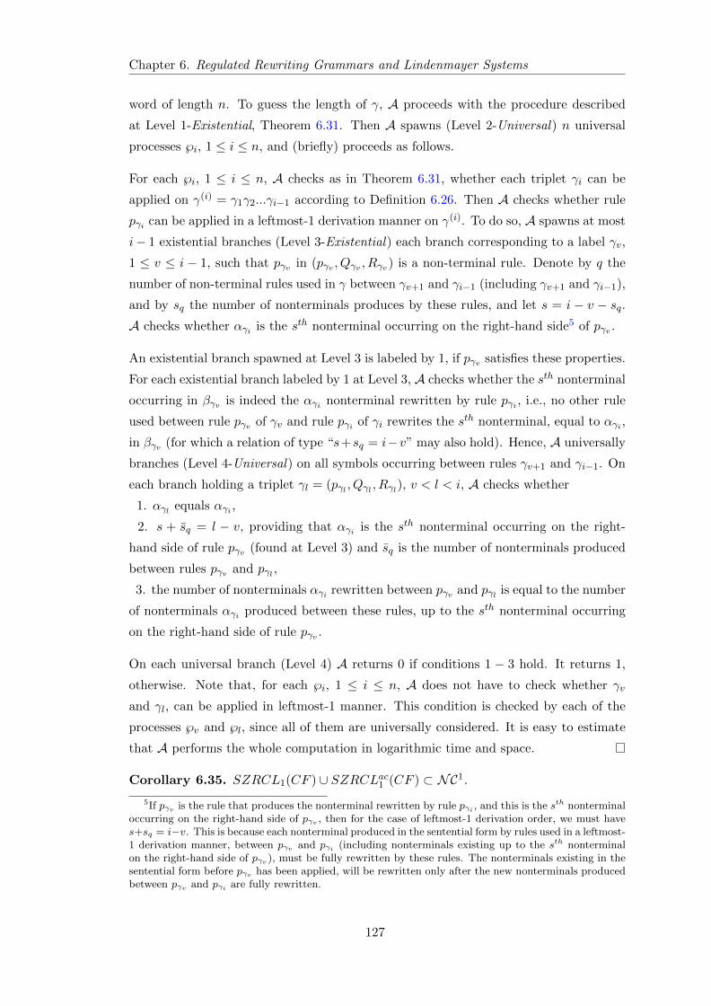
Chapter 6. Regulated Rewriting Grammars and Lindenmayer Systems
word of length n. To guess the length of γ, A proceeds with the procedure described
at Level 1-Existential, Theorem 6.31. Then A spawns (Level 2-Universal) n universal
processes ℘i, 1 ≤ i ≤ n, and (briefly) proceeds as follows.
For each ℘i, 1 ≤ i ≤ n, A checks as in Theorem 6.31, whether each triplet γi can be
applied on γ(i) = γ1γ2...γi−1 according to Definition 6.26. Then A checks whether rule
pγi can be applied in a leftmost-1 derivation manner on γ(i). To do so, A spawns at most
i− 1 existential branches (Level 3-Existential) each branch corresponding to a label γv,
1 ≤ v ≤ i − 1, such that pγv in (pγv , Qγv , Rγv) is a non-terminal rule. Denote by q the
number of non-terminal rules used in γ between γv+1 and γi−1 (including γv+1 and γi−1),
and by sq the number of nonterminals produces by these rules, and let s = i − v − sq.A checks whether αγi is the sth nonterminal occurring on the right-hand side5 of pγv .
An existential branch spawned at Level 3 is labeled by 1, if pγv satisfies these properties.
For each existential branch labeled by 1 at Level 3, A checks whether the sth nonterminal
occurring in βγv is indeed the αγi nonterminal rewritten by rule pγi , i.e., no other rule
used between rule pγv of γv and rule pγi of γi rewrites the sth nonterminal, equal to αγi ,
in βγv (for which a relation of type “s+sq = i−v” may also hold). Hence, A universally
branches (Level 4-Universal) on all symbols occurring between rules γv+1 and γi−1. On
each branch holding a triplet γl = (pγl , Qγl , Rγl), v < l < i, A checks whether
1. αγl equals αγi ,
2. s + sq = l − v, providing that αγi is the sth nonterminal occurring on the right-
hand side of rule pγv (found at Level 3) and sq is the number of nonterminals produced
between rules pγv and pγl ,
3. the number of nonterminals αγi rewritten between pγv and pγl is equal to the number
of nonterminals αγi produced between these rules, up to the sth nonterminal occurring
on the right-hand side of rule pγv .
On each universal branch (Level 4) A returns 0 if conditions 1 − 3 hold. It returns 1,
otherwise. Note that, for each ℘i, 1 ≤ i ≤ n, A does not have to check whether γv
and γl, can be applied in leftmost-1 manner. This condition is checked by each of the
processes ℘v and ℘l, since all of them are universally considered. It is easy to estimate
that A performs the whole computation in logarithmic time and space.
Corollary 6.35. SZRCL1(CF ) ∪ SZRCLac1 (CF ) ⊂ NC1.
5If pγv is the rule that produces the nonterminal rewritten by rule pγi , and this is the sth nonterminaloccurring on the right-hand side of pγv , then for the case of leftmost-1 derivation order, we must haves+sq = i−v. This is because each nonterminal produced in the sentential form by rules used in a leftmost-1 derivation manner, between pγv and pγi (including nonterminals existing up to the sth nonterminalon the right-hand side of pγv ), must be fully rewritten by these rules. The nonterminals existing in thesentential form before pγv has been applied, will be rewritten only after the new nonterminals producedbetween pγv and pγi are fully rewritten.
127
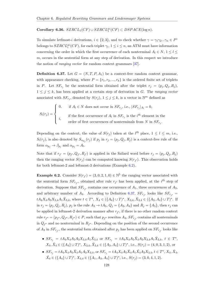
Chapter 6. Regulated Rewriting Grammars and Lindenmayer Systems
Corollary 6.36. SZRCL1(CF ) ∪ SZRCLac1 (CF ) ⊂ DSPACE(log n).
To simulate letfmost-i derivations, i ∈ 2, 3, and to check whether γ = γ1γ2...γn ∈ P ∗
belongs to SZRCLaci (CF ), for each triplet γi, 1 ≤ i ≤ n, an ATM must have information
concerning the order in which the first occurrence of each nonterminal Al ∈ N , 1 ≤ l ≤m, occurs in the sentential form at any step of derivation. In this respect we introduce
the notion of ranging vector for random context grammars [37].
Definition 6.37. Let G = (N,T, P,A1) be a context-free random context grammar,
with appearance checking, where P = r1, r2, ..., rk is the ordered finite set of triplets
in P . Let SFrj be the sentential form obtained after the triplet rj = (pj , Qj , Rj),
1 ≤ j ≤ k, has been applied at a certain step of derivation in G. The ranging vector
associated with SFrj , denoted by S(rj), 1 ≤ j ≤ k, is a vector in Nm defined as
Sl(rj) =
0, if Al ∈ N does not occur in SFrj , i.e., |SFrj |Al = 0,
i,if the first occurrence of Al in SFrj is the ith element in the
order of first occurrences of nonterminals from N in SFrj .
Depending on the context, the value of S(rj) taken at the lth place, 1 ≤ l ≤ m, i.e.,
Sl(rj), is also denoted by Sαpj (rj) if pj in rj = (pj , Qj , Rj) is a context-free rule of the
form αpj → βpj and αpj = Al.
Note that if rj′ = (pj′ , Qj′ , Rj′) is applied in the Szilard word before rj = (pj , Qj , Rj)
then the ranging vector S(rj) can be computed knowing S(rj′). This observation holds
for both leftmost-2 and leftmost-3 derivations (Example 6.2).
Example 6.2. Consider S(rj′) = (3, 0, 2, 1, 0) ∈ N5 the ranging vector associated with
the sentential form SFrj′ , obtained after rule rj′ has been applied, at the ith step of
derivation. Suppose that SFrj′ contains one occurrence of A1, three occurrences of A3,
and arbitrary number of A4. According to Definition 6.37, SFrj′ looks like SFrj′ =
tA4X4A3X3,4A1X3,4, where t ∈ T ∗, X4 ∈ (A4 ∪ T )∗, X3,4, X3,4 ∈ (A3, A4 ∪ T )∗. If
in rj = (pj , Qj , Rj), pj is the rule A3 → tA5, Qj = A3, A4 and Rj = A5, then rj can
be applied in leftmost-2 derivation manner after rj′ , if there is no other random context
rule rj′′ = (pj′′ , Qj′′ , Rj′′) ∈ P , such that pj′′ rewrites A4, SFrj′ contains all nonterminals
in Qj′′ and no nonterminal in Rj′′ . Depending on the position of the second occurrence
of A3 in SFrj′ , the sentential form obtained after pj has been applied on SFrj′ looks like
• SFrj = tA4X4A5A3X3,4A1X3,4 or SFrj = tA4X4A5X4A3X3,4A1X3,4, t ∈ T ∗,
X4, X4 ∈ (A4 ∪ T )∗, X3,4, X3,4 ∈ (A3, A4 ∪ T )∗, i.e., S(rj) = (4, 0, 3, 1, 2), or
• SFrj = tA4X4A5X4A1A3X3,4, or SFrj = tA4X4A5X4A1X4A3X3,4, t ∈ T ∗, X4, X4,
X4 ∈ (A4 ∪ T )∗, X3,4 ∈ (A1, A3, A4 ∪ T )∗, i.e., S(rj) = (3, 0, 4, 1, 2).
128
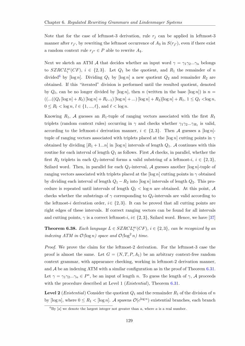
Chapter 6. Regulated Rewriting Grammars and Lindenmayer Systems
Note that for the case of leftmost-3 derivation, rule rj can be applied in leftmost-3
manner after rj′ , by rewriting the leftmost occurrence of A3 in S(rj′), even if there exist
a random context rule rj′′ ∈ P able to rewrite A4.
Next we sketch an ATM A that decides whether an input word γ = γ1γ2...γn belongs
to SZRCLaci (CF ), i ∈ 2, 3. Let Q1 be the quotient, and R1 the remainder of n
divided6 by [log n]. Dividing Q1 by [log n] a new quotient Q2 and remainder R2 are
obtained. If this “iterated” division is performed until the resulted quotient, denoted
by Q`, can be no longer divided by [log n], then n (written in the base [log n]) is n =
((...((Q` [log n] +R`) [log n] +R`−1) [log n] + ...) [log n] +R2)[log n] +R1, 1 ≤ Q` <log n,
0 ≤ Rl < log n, l ∈ 1, ..., `, and ` < log n.
Knowing R1, A guesses an R1-tuple of ranging vectors associated with the first R1
triplets (random context rules) occurring in γ and checks whether γ1γ2...γR1 is valid,
according to the leftmost-i derivation manner, i ∈ 2, 3. Then A guesses a [log n]-
tuple of ranging vectors associated with triplets placed at the [log n] cutting points in γ
obtained by dividing [R1 + 1...n] in [log n] intervals of length Q1. A continues with this
routine for each interval of length Q1 as follows. First A checks, in parallel, whether the
first R2 triplets in each Q1-interval forms a valid substring of a leftmost-i, i ∈ 2, 3,Szilard word. Then, in parallel for each Q1-interval, A guesses another [log n]-tuple of
ranging vectors associated with triplets placed at the [log n] cutting points in γ obtained
by dividing each interval of length Q1−R2 into [log n] intervals of length Q2. This pro-
cedure is repeated until intervals of length Q` < log n are obtained. At this point, Achecks whether the substrings of γ corresponding to Q`-intervals are valid according to
the leftmost-i derivation order, i∈ 2, 3. It can be proved that all cutting points are
right edges of these intervals. If correct ranging vectors can be found for all intervals
and cutting points, γ is a correct leftmost-i, i∈ 2, 3, Szilard word. Hence, we have [37]
Theorem 6.38. Each language L ∈ SZRCLaci (CF ), i ∈ 2, 3, can be recognized by an
indexing ATM in O(log n) space and O(log2 n) time.
Proof. We prove the claim for the leftmost-2 derivation. For the leftmost-3 case the
proof is almost the same. Let G = (N,T, P,A1) be an arbitrary context-free random
context grammar, with appearance checking, working in leftmost-2 derivation manner,
and A be an indexing ATM with a similar configuration as in the proof of Theorem 6.31.
Let γ = γ1γ2...γn ∈ P ∗, be an input of length n. To guess the length of γ, A proceeds
with the procedure described at Level 1 (Existential), Theorem 6.31.
Level 2 (Existential) Consider the quotient Q1 and the remainder R1 of the division of n
by [log n], where 0 ≤ R1 < [log n]. A spawns O(clogn) existential branches, each branch
6By [a] we denote the largest integer not greater than a, where a is a real number.
129
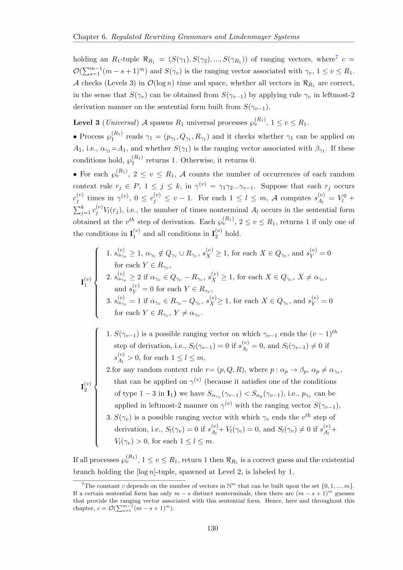
Chapter 6. Regulated Rewriting Grammars and Lindenmayer Systems
holding an R1-tuple <R1 = (S(γ1), S(γ2), ..., S(γR1)) of ranging vectors, where7 c =
O(∑m−1
s=1 (m− s+ 1)m) and S(γv) is the ranging vector associated with γv, 1 ≤ v ≤ R1.
A checks (Levels 3) in O(log n) time and space, whether all vectors in <R1 are correct,
in the sense that S(γv) can be obtained from S(γv−1) by applying rule γv in leftmost-2
derivation manner on the sentential form built from S(γv−1).
Level 3 (Universal) A spawns R1 universal processes ℘(R1)v , 1 ≤ v ≤ R1.
• Process ℘(R1)1 reads γ1 = (pγ1 , Qγ1 , Rγ1) and it checks whether γ1 can be applied on
A1, i.e., αγ1 =A1, and whether S(γ1) is the ranging vector associated with βγ1 . If these
conditions hold, ℘(R1)1 returns 1. Otherwise, it returns 0.
• For each ℘(R1)v , 2 ≤ v ≤ R1, A counts the number of occurrences of each random
context rule rj ∈ P , 1 ≤ j ≤ k, in γ(v) = γ1γ2...γv−1. Suppose that each rj occurs
c(v)j times in γ(v), 0 ≤ c
(v)j ≤ v − 1. For each 1 ≤ l ≤ m, A computes s
(v)Al
= V 0l +∑k
j=1 c(v)j Vl(rj), i.e., the number of times nonterminal Al occurs in the sentential form
obtained at the vth step of derivation. Each ℘(R1)v , 2 ≤ v ≤ R1, returns 1 if only one of
the conditions in I(v)1 and all conditions in I
(v)2 hold.
I(v)1
1. s(v)αγv ≥ 1, αγv /∈ Qγv ∪Rγv , s
(v)X ≥ 1, for each X ∈ Qγv , and s
(v)Y = 0
for each Y ∈ Rγv ,2. s
(v)αγv ≥ 2 if αγv ∈ Qγv −Rγv , s
(v)X ≥ 1, for each X ∈ Qγv , X 6= αγv ,
and s(v)Y = 0 for each Y ∈ Rγv ,
3. s(v)αγv = 1 if αγv ∈ Rγv−Qγv , s
(v)X ≥ 1, for each X ∈ Qγv , and s
(v)Y = 0
for each Y ∈ Rγv , Y 6= αγv .
I(v)2
1. S(γv−1) is a possible ranging vector on which γv−1 ends the (v − 1)th
step of derivation, i.e., Sl(γv−1) = 0 if s(v)Al
= 0, and Sl(γv−1) 6= 0 if
s(v)Al
> 0, for each 1 ≤ l ≤ m,
2.for any random context rule r= (p,Q,R), where p : αp → βp, αp 6= αγv ,
that can be applied on γ(v) (because it satisfies one of the conditions
of type 1− 3 in I1) we have Sαγv (γv−1) < Sαp(γv−1), i.e., pγv can be
applied in leftmost-2 manner on γ(v) with the ranging vector S(γv−1),
3. S(γv) is a possible ranging vector with which γv ends the vth step of
derivation, i.e., Sl(γv) = 0 if s(v)Al
+ Vl(γv) = 0, and Sl(γv) 6= 0 if s(v)Al
+
Vl(γv) > 0, for each 1 ≤ l ≤ m.
If all processes ℘(R1)v , 1 ≤ v ≤ R1, return 1 then <R1 is a correct guess and the existential
branch holding the [log n]-tuple, spawned at Level 2, is labeled by 1.
7The constant c depends on the number of vectors in Nm that can be built upon the set 0, 1, ...,m.If a certain sentential form has only m − s distinct nonterminals, then there are (m − s + 1)m guessesthat provide the ranging vector associated with this sentential form. Hence, here and throughout thischapter, c = O(
∑m−1s=1 (m− s+ 1)m).
130

Chapter 6. Regulated Rewriting Grammars and Lindenmayer Systems
Level 4 (Existential) Let Q2 be the quotient and R2 the remainder of Q1 divided by
[log n], 0 ≤ R2 < [log n]. A spawns O(clogn) existential branches, each branch holding a
2 [log n]-tuple <cR2=(S(γR1), S(γR1+R2), S(γR1+Q1), S(γR1+Q1+R2), ..., S(γR1+([logn]−1)Q1
),
S(γR1+([logn]−1)Q1+R2)), where S(γR1) is the ranging vector belonging to the R1-tuple
found correct at Level 3. Because the tuple <R1 is not useful anymore, the space used
by A to record <R1 is allocated now to record <cR2.
Level 5 (Universal) On each existential branch from Level 4, A spawns [log n] uni-
versal processes ℘(Q1)i1
, 0 ≤ i1 ≤ [log n] − 1. Each process ℘(Q1)i1
takes the interval
[R1 + i1Q1...R1 + i1Q1 + R2], and checks whether the ranging vectors S(γR1+i1Q1) and
S(γR1+i1Q1+R2), 1 ≤ i1 ≤ [log n] − 1, provide a correct order in which the leftmost-2
derivation can be performed between γR1+i1Q1 and γR1+i1Q1+R2 . Besides S(γR1+i1Q1)
and S(γR1+i1Q1+R2), each ℘(Q1)i1
also keeps, from the previous level, the ranging vector
S(γR1+(i1+1)Q1). In this way each ranging vector S(γR1+i1Q1), 1 ≤ i1 ≤ [log n] − 1,
guessed at Level 4, is redirected to only one process, i.e., ℘(Q1)i1−1. Denote by xi1 =
R1 + i1Q1, 0 ≤ i1 ≤ [log n]− 1.
Level 6 (Existential) For each universal process ℘(Q1)i1
, 0 ≤ i1 ≤ [log n] − 1, A spawns
O(clogn) existential branches, each branch holding an (R2 + 1)-tuple of ranging vec-
tors <R2 = (S(γxi1 ), S(γxi1+1), ..., S(γxi1+R2−1), S(γxi1+R2)). Then A checks whether
all vectors in <R2 are correct ranging vectors according to the leftmost-2 derivation re-
quirements. This can be done, for each process ℘(Q1)i1
, 0 ≤ i1 ≤ [log n] − 1, in O(log n)
time and space, through Level 7 as follows.
Level 7 (Universal) For each existential branch spawned at Level 6, A spawns R2 uni-
versal processes ℘(R2)v , 1 ≤ v ≤ R2. On each ℘
(R2)v , A checks whether each substring
γxi1γxi1+1...γxi1+v is correct according to the leftmost-2 derivation order. In this re-
spect, for each ℘(R2)v , 1 ≤ v ≤ R2, A counts the number of occurrences of each random
context rule rj ∈ P , 1 ≤ j ≤ k, in γ(i1,v) = γ1γ2...γxi1+v−1. Suppose that each rj occurs
c(i1,v)j times, 0 ≤ c
(i1,v)j ≤ xi1 + v − 1, in γ(i1,v). For each 1 ≤ l ≤ m, A computes
s(i1,v)Al
= V 0l +
∑kj=1 c
(i1,v)j Vl(rj), i.e., the number of times Al occurs in the sentential
form obtained at the (xi1 + v)th step of derivation. Then A checks conditions of type
I(v)1 and I
(v)2 (Level 3) for the random context rule γxi1+v, i.e., instead of v, xi1 + v is
considered. Denote by I(i1,v)1 and I
(i1,v)2 these conditions.
Each ℘(R2)v , 1 ≤ v ≤ R2, is said partially correct if one of the conditions in I
(i1,v)1 and all
conditions in I(i1,v)2 hold. If ℘
(R2)v is not partially correct, it is labeled by 0. Note that, at
this moment we cannot decide whether ℘(R2)v can be labeled by 1, since we do not know
whether S(γxi1 ) is valid, i.e., whether γxi1 indeed ends the xthi1 step of derivation with
the ranging vector S(γxi1 ), and whether γxi1 can be applied in the leftmost-2 derivation
131
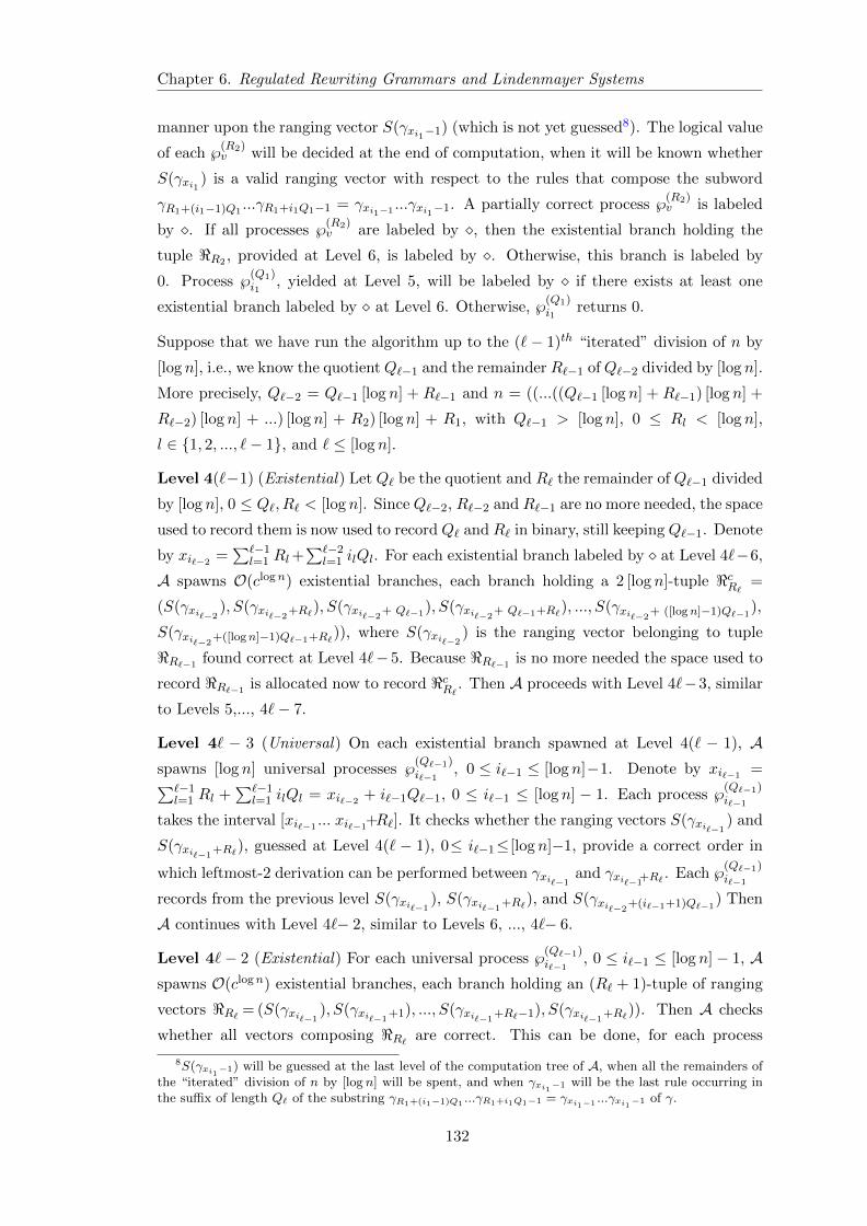
Chapter 6. Regulated Rewriting Grammars and Lindenmayer Systems
manner upon the ranging vector S(γxi1−1) (which is not yet guessed8). The logical value
of each ℘(R2)v will be decided at the end of computation, when it will be known whether
S(γxi1 ) is a valid ranging vector with respect to the rules that compose the subword
γR1+(i1−1)Q1...γR1+i1Q1−1 = γxi1−1 ...γxi1−1. A partially correct process ℘
(R2)v is labeled
by . If all processes ℘(R2)v are labeled by , then the existential branch holding the
tuple <R2 , provided at Level 6, is labeled by . Otherwise, this branch is labeled by
0. Process ℘(Q1)i1
, yielded at Level 5, will be labeled by if there exists at least one
existential branch labeled by at Level 6. Otherwise, ℘(Q1)i1
returns 0.
Suppose that we have run the algorithm up to the (`− 1)th “iterated” division of n by
[log n], i.e., we know the quotientQ`−1 and the remainder R`−1 ofQ`−2 divided by [log n].
More precisely, Q`−2 = Q`−1 [log n] + R`−1 and n = ((...((Q`−1 [log n] + R`−1) [log n] +
R`−2) [log n] + ...) [log n] + R2) [log n] + R1, with Q`−1 > [log n], 0 ≤ Rl < [log n],
l ∈ 1, 2, ..., `− 1, and ` ≤ [log n].
Level 4(`−1) (Existential) Let Q` be the quotient and R` the remainder of Q`−1 divided
by [log n], 0 ≤ Q`, R` < [log n]. Since Q`−2, R`−2 and R`−1 are no more needed, the space
used to record them is now used to record Q` and R` in binary, still keeping Q`−1. Denote
by xi`−2=∑`−1
l=1 Rl+∑`−2
l=1 ilQl. For each existential branch labeled by at Level 4`−6,
A spawns O(clogn) existential branches, each branch holding a 2 [log n]-tuple <cR` =
(S(γxi`−2), S(γxi`−2
+R`), S(γxi`−2+ Q`−1
), S(γxi`−2+ Q`−1+R`), ..., S(γxi`−2
+ ([logn]−1)Q`−1),
S(γxi`−2+([logn]−1)Q`−1+R`)), where S(γxi`−2
) is the ranging vector belonging to tuple
<R`−1found correct at Level 4`− 5. Because <R`−1
is no more needed the space used to
record <R`−1is allocated now to record <cR` . Then A proceeds with Level 4`−3, similar
to Levels 5,..., 4`− 7.
Level 4` − 3 (Universal) On each existential branch spawned at Level 4(` − 1), Aspawns [log n] universal processes ℘
(Q`−1)i`−1
, 0 ≤ i`−1 ≤ [log n]−1. Denote by xi`−1=∑`−1
l=1 Rl +∑`−1
l=1 ilQl = xi`−2+ i`−1Q`−1, 0 ≤ i`−1 ≤ [log n] − 1. Each process ℘
(Q`−1)i`−1
takes the interval [xi`−1... xi`−1
+R`]. It checks whether the ranging vectors S(γxi`−1) and
S(γxi`−1+R`), guessed at Level 4(` − 1), 0≤ i`−1≤ [log n]−1, provide a correct order in
which leftmost-2 derivation can be performed between γxi`−1and γxi`−1
+R` . Each ℘(Q`−1)i`−1
records from the previous level S(γxi`−1), S(γxi`−1
+R`), and S(γxi`−2+(i`−1+1)Q`−1
) Then
A continues with Level 4`− 2, similar to Levels 6, ..., 4`− 6.
Level 4`− 2 (Existential) For each universal process ℘(Q`−1)i`−1
, 0 ≤ i`−1 ≤ [log n]− 1, Aspawns O(clogn) existential branches, each branch holding an (R` + 1)-tuple of ranging
vectors <R` = (S(γxi`−1), S(γxi`−1
+1), ..., S(γxi`−1+R`−1), S(γxi`−1
+R`)). Then A checks
whether all vectors composing <R` are correct. This can be done, for each process
8S(γxi1−1) will be guessed at the last level of the computation tree of A, when all the remainders ofthe “iterated” division of n by [logn] will be spent, and when γxi1−1 will be the last rule occurring inthe suffix of length Q` of the substring γR1+(i1−1)Q1
...γR1+i1Q1−1 = γxi1−1 ...γxi1−1 of γ.
132
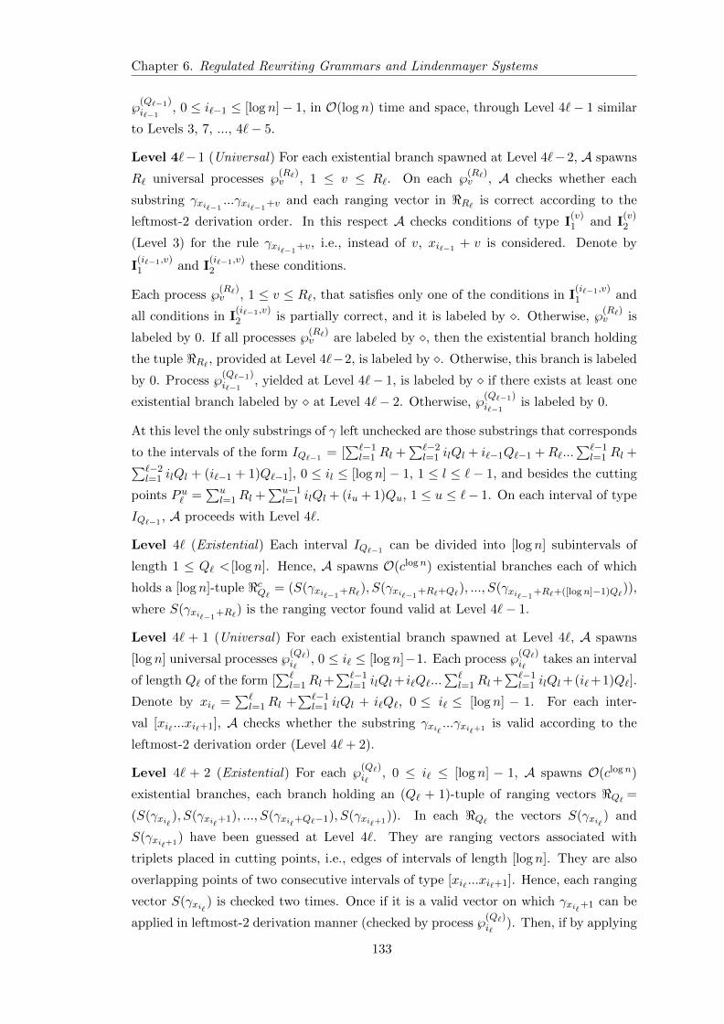
Chapter 6. Regulated Rewriting Grammars and Lindenmayer Systems
℘(Q`−1)i`−1
, 0 ≤ i`−1 ≤ [log n]− 1, in O(log n) time and space, through Level 4`− 1 similar
to Levels 3, 7, ..., 4`− 5.
Level 4`−1 (Universal) For each existential branch spawned at Level 4`−2, A spawns
R` universal processes ℘(R`)v , 1 ≤ v ≤ R`. On each ℘
(R`)v , A checks whether each
substring γxi`−1...γxi`−1
+v and each ranging vector in <R` is correct according to the
leftmost-2 derivation order. In this respect A checks conditions of type I(v)1 and I
(v)2
(Level 3) for the rule γxi`−1+v, i.e., instead of v, xi`−1
+ v is considered. Denote by
I(i`−1,v)1 and I
(i`−1,v)2 these conditions.
Each process ℘(R`)v , 1 ≤ v ≤ R`, that satisfies only one of the conditions in I
(i`−1,v)1 and
all conditions in I(i`−1,v)2 is partially correct, and it is labeled by . Otherwise, ℘
(R`)v is
labeled by 0. If all processes ℘(R`)v are labeled by , then the existential branch holding
the tuple <R` , provided at Level 4`−2, is labeled by . Otherwise, this branch is labeled
by 0. Process ℘(Q`−1)i`−1
, yielded at Level 4`− 1, is labeled by if there exists at least one
existential branch labeled by at Level 4`− 2. Otherwise, ℘(Q`−1)i`−1
is labeled by 0.
At this level the only substrings of γ left unchecked are those substrings that corresponds
to the intervals of the form IQ`−1= [∑`−1
l=1 Rl +∑`−2
l=1 ilQl + i`−1Q`−1 +R`...∑`−1
l=1 Rl +∑`−2l=1 ilQl + (i`−1 + 1)Q`−1], 0 ≤ il ≤ [log n]− 1, 1 ≤ l ≤ `− 1, and besides the cutting
points P u` =∑u
l=1Rl +∑u−1
l=1 ilQl + (iu + 1)Qu, 1 ≤ u ≤ `− 1. On each interval of type
IQ`−1, A proceeds with Level 4`.
Level 4` (Existential) Each interval IQ`−1can be divided into [log n] subintervals of
length 1 ≤ Q` < [log n]. Hence, A spawns O(clogn) existential branches each of which
holds a [log n]-tuple <cQ` = (S(γxi`−1+R`), S(γxi`−1
+R`+Q`), ..., S(γxi`−1+R`+([logn]−1)Q`)),
where S(γxi`−1+R`) is the ranging vector found valid at Level 4`− 1.
Level 4` + 1 (Universal) For each existential branch spawned at Level 4`, A spawns
[log n] universal processes ℘(Q`)i`
, 0 ≤ i` ≤ [log n]−1. Each process ℘(Q`)i`
takes an interval
of length Q` of the form [∑`
l=1Rl+∑`−1
l=1 ilQl+ i`Q`...∑`
l=1Rl+∑`−1
l=1 ilQl+(i`+1)Q`].
Denote by xi` =∑`
l=1Rl +∑`−1
l=1 ilQl + i`Q`, 0 ≤ i` ≤ [log n] − 1. For each inter-
val [xi` ...xi`+1], A checks whether the substring γxi` ...γxi`+1 is valid according to the
leftmost-2 derivation order (Level 4`+ 2).
Level 4` + 2 (Existential) For each ℘(Q`)i`
, 0 ≤ i` ≤ [log n] − 1, A spawns O(clogn)
existential branches, each branch holding an (Q` + 1)-tuple of ranging vectors <Q` =
(S(γxi` ), S(γxi`+1), ..., S(γxi`+Q`−1), S(γxi`+1)). In each <Q` the vectors S(γxi` ) and
S(γxi`+1) have been guessed at Level 4`. They are ranging vectors associated with
triplets placed in cutting points, i.e., edges of intervals of length [log n]. They are also
overlapping points of two consecutive intervals of type [xi` ...xi`+1]. Hence, each ranging
vector S(γxi` ) is checked two times. Once if it is a valid vector on which γxi`+1 can be
applied in leftmost-2 derivation manner (checked by process ℘(Q`)i`
). Then, if by applying
133
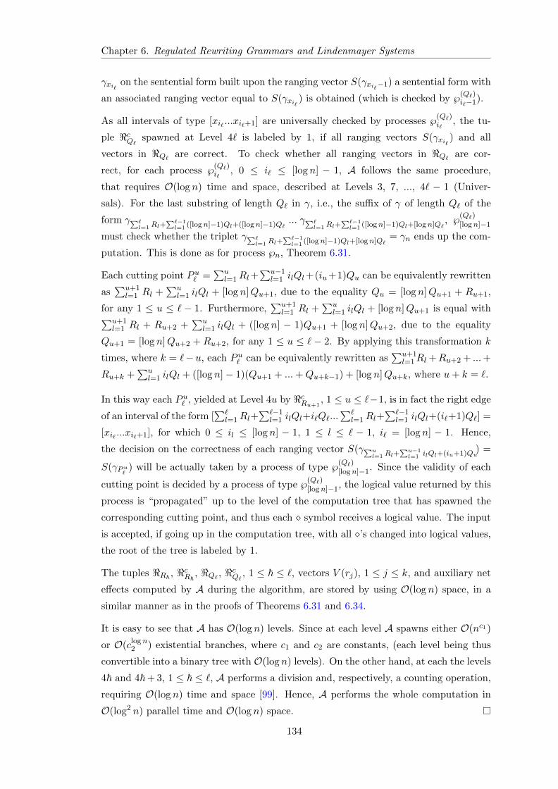
Chapter 6. Regulated Rewriting Grammars and Lindenmayer Systems
γxi` on the sentential form built upon the ranging vector S(γxi`−1) a sentential form with
an associated ranging vector equal to S(γxi` ) is obtained (which is checked by ℘(Q`)i`−1).
As all intervals of type [xi` ...xi`+1] are universally checked by processes ℘(Q`)i`
, the tu-
ple <cQ` spawned at Level 4` is labeled by 1, if all ranging vectors S(γxi` ) and all
vectors in <Q` are correct. To check whether all ranging vectors in <Q` are cor-
rect, for each process ℘(Q`)i`
, 0 ≤ i` ≤ [log n] − 1, A follows the same procedure,
that requires O(log n) time and space, described at Levels 3, 7, ..., 4` − 1 (Univer-
sals). For the last substring of length Q` in γ, i.e., the suffix of γ of length Q` of the
form γ∑`l=1 Rl+
∑`−1l=1 ([logn]−1)Ql+([logn]−1)Q`
... γ∑`l=1Rl+
∑`−1l=1 ([logn]−1)Ql+[logn]Q`
, ℘(Q`)[logn]−1
must check whether the triplet γ∑`l=1Rl+
∑`−1l=1 ([logn]−1)Ql+[logn]Q`
= γn ends up the com-
putation. This is done as for process ℘n, Theorem 6.31.
Each cutting point P u` =∑u
l=1Rl+∑u−1
l=1 ilQl+(iu+1)Qu can be equivalently rewritten
as∑u+1
l=1 Rl +∑u
l=1 ilQl + [log n]Qu+1, due to the equality Qu = [log n]Qu+1 + Ru+1,
for any 1 ≤ u ≤ ` − 1. Furthermore,∑u+1
l=1 Rl +∑u
l=1 ilQl + [log n]Qu+1 is equal with∑u+1l=1 Rl + Ru+2 +
∑ul=1 ilQl + ([log n] − 1)Qu+1 + [log n]Qu+2, due to the equality
Qu+1 = [log n]Qu+2 + Ru+2, for any 1 ≤ u ≤ ` − 2. By applying this transformation k
times, where k = `−u, each P u` can be equivalently rewritten as∑u+1
l=1Rl +Ru+2 + ...+
Ru+k +∑u
l=1 ilQl + ([log n]− 1)(Qu+1 + ...+Qu+k−1) + [log n]Qu+k, where u+ k = `.
In this way each P u` , yielded at Level 4u by <cRu+1, 1 ≤ u ≤ `−1, is in fact the right edge
of an interval of the form [∑`
l=1Rl+∑`−1
l=1 ilQl+i`Q`...∑`
l=1Rl+∑`−1
l=1 ilQl+(i`+1)Q`] =
[xi` ...xi`+1], for which 0 ≤ il ≤ [log n] − 1, 1 ≤ l ≤ ` − 1, i` = [log n] − 1. Hence,
the decision on the correctness of each ranging vector S(γ∑ul=1Rl+
∑u−1l=1 ilQl+(iu+1)Qu
) =
S(γPu` ) will be actually taken by a process of type ℘(Q`)[logn]−1. Since the validity of each
cutting point is decided by a process of type ℘(Q`)[logn]−1, the logical value returned by this
process is “propagated” up to the level of the computation tree that has spawned the
corresponding cutting point, and thus each symbol receives a logical value. The input
is accepted, if going up in the computation tree, with all ’s changed into logical values,
the root of the tree is labeled by 1.
The tuples <R~ , <cR~, <Q` , <cQ` , 1 ≤ ~ ≤ `, vectors V (rj), 1 ≤ j ≤ k, and auxiliary net
effects computed by A during the algorithm, are stored by using O(log n) space, in a
similar manner as in the proofs of Theorems 6.31 and 6.34.
It is easy to see that A has O(log n) levels. Since at each level A spawns either O(nc1)
or O(clogn2 ) existential branches, where c1 and c2 are constants, (each level being thus
convertible into a binary tree with O(log n) levels). On the other hand, at each the levels
4~ and 4~+ 3, 1 ≤ ~ ≤ `, A performs a division and, respectively, a counting operation,
requiring O(log n) time and space [99]. Hence, A performs the whole computation in
O(log2 n) parallel time and O(log n) space.
134
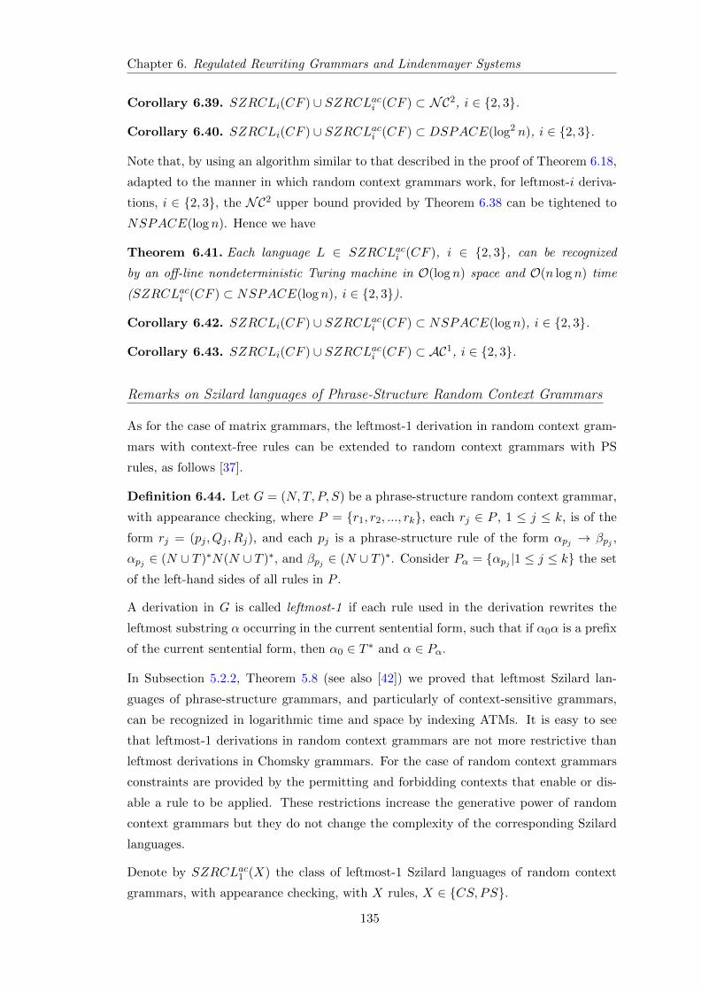
Chapter 6. Regulated Rewriting Grammars and Lindenmayer Systems
Corollary 6.39. SZRCLi(CF ) ∪ SZRCLaci (CF ) ⊂ NC2, i ∈ 2, 3.
Corollary 6.40. SZRCLi(CF ) ∪ SZRCLaci (CF ) ⊂ DSPACE(log2 n), i ∈ 2, 3.
Note that, by using an algorithm similar to that described in the proof of Theorem 6.18,
adapted to the manner in which random context grammars work, for leftmost-i deriva-
tions, i ∈ 2, 3, the NC2 upper bound provided by Theorem 6.38 can be tightened to
NSPACE(log n). Hence we have
Theorem 6.41. Each language L ∈ SZRCLaci (CF ), i ∈ 2, 3, can be recognized
by an off-line nondeterministic Turing machine in O(log n) space and O(n log n) time
(SZRCLaci (CF ) ⊂ NSPACE(log n), i ∈ 2, 3).
Corollary 6.42. SZRCLi(CF ) ∪ SZRCLaci (CF ) ⊂ NSPACE(log n), i ∈ 2, 3.
Corollary 6.43. SZRCLi(CF ) ∪ SZRCLaci (CF ) ⊂ AC1, i ∈ 2, 3.
Remarks on Szilard languages of Phrase-Structure Random Context Grammars
As for the case of matrix grammars, the leftmost-1 derivation in random context gram-
mars with context-free rules can be extended to random context grammars with PS
rules, as follows [37].
Definition 6.44. Let G = (N,T, P, S) be a phrase-structure random context grammar,
with appearance checking, where P = r1, r2, ..., rk, each rj ∈ P , 1 ≤ j ≤ k, is of the
form rj = (pj , Qj , Rj), and each pj is a phrase-structure rule of the form αpj → βpj ,
αpj ∈ (N ∪ T )∗N(N ∪ T )∗, and βpj ∈ (N ∪ T )∗. Consider Pα = αpj |1 ≤ j ≤ k the set
of the left-hand sides of all rules in P .
A derivation in G is called leftmost-1 if each rule used in the derivation rewrites the
leftmost substring α occurring in the current sentential form, such that if α0α is a prefix
of the current sentential form, then α0 ∈ T ∗ and α ∈ Pα.
In Subsection 5.2.2, Theorem 5.8 (see also [42]) we proved that leftmost Szilard lan-
guages of phrase-structure grammars, and particularly of context-sensitive grammars,
can be recognized in logarithmic time and space by indexing ATMs. It is easy to see
that leftmost-1 derivations in random context grammars are not more restrictive than
leftmost derivations in Chomsky grammars. For the case of random context grammars
constraints are provided by the permitting and forbidding contexts that enable or dis-
able a rule to be applied. These restrictions increase the generative power of random
context grammars but they do not change the complexity of the corresponding Szilard
languages.
Denote by SZRCLac1 (X) the class of leftmost-1 Szilard languages of random context
grammars, with appearance checking, with X rules, X ∈ CS,PS.
135
Chapter 6. Regulated Rewriting Grammars and Lindenmayer Systems
Theorem 6.45. SZRCLac1 (X) ⊆ ALOGTIME, X ∈ CS,PS.
Proof. The claim can be proved by using a similar method as in the proof of Theorem 5.8
(Subsection 5.2.2) in which additionally, for each random context rule γi of the form
(pγi , Qγi , Rγi), 1 ≤ i ≤ n, occurring in the input word γ = γ1γ2...γn ∈ P ∗, A checks,
besides the leftmost-1 conditions, also whether the sentential form obtained at the ith
step of derivation, denoted by SFi, contains all nonterminals in Qγi and no nonterminal
in Rγi (by omitting to count common occurrences of a nonterminal on SFi and on the
left-hand side of rule pγi).
Corollary 6.46. SZRCL1(X)∪SZRCLac1 (X) ⊂ NC1 (SZRCL1(X)∪SZRCLac1 (X) ⊂DSPACE(log n)), X ∈ CS,PS.
6.2.4 Conclusions and Further Investigations
In Section 6.2 we have investigated the complexity of unrestricted and leftmost-like Szi-
lard languages of random context grammars, with or without appearance checking. We
proved that the class of unrestricted Szilard languages of context-free random context
grammars with appearance checking can be accepted by an indexing ATM in logarith-
mic time and space (Theorem 6.31). The same result holds for the class of leftmost-1
Szilard languages of context-free random context grammars, with appearance checking
(Theorem 6.34). Consequently, these classes of Szilard languages are contained in NC1.
The classes of leftmost-i Szilard languages, i ∈ 2, 3, of context-free random context
grammars with appearance checking can be recognized by an indexing ATM by using
logarithmic space and square logarithmic time (Theorem 6.38). Hence, these classes of
leftmost Szilard languages are contained in NC2.
Using a similar technique as in the proof of Theorem 6.18, it can be proved that the
classes of leftmost-i Szilard languages, i ∈ 2, 3, of context-free random context gram-
mars with appearance checking can be recognized by an off-line nondeterministic Turing
machine in O(log n) space and O(n log n) time (Theorem 6.41), hence the NC2 upper
bound can be tightened to NSPACE(log n), and therefore to AC1.
As a consequence of Theorem 5.8 (Subsection 5.2.2) the class of leftmost-1 Szilard lan-
guages of random context grammars, with appearance checking, with phrase-structure
rules, is contained in NC1 (Theorem 6.45).
The results in Section 6.2 are gathered from [36, 37]. We have no results concerning
the complexity of leftmost-i, i ∈ 2, 3, Szilard languages of random context grammars
with or without appearance checking with phrase-structure rules. These problems are
left open for further investigations.
136
Chapter 6. Regulated Rewriting Grammars and Lindenmayer Systems
6.3 Programmed Grammars
6.3.1 Prerequisites
A programmed grammar is a regulated rewriting grammar in which the application of
a rule is conditioned by its occurrence in the so called success field associated with the
rule previously applied in the derivation. If a rule is effectively applied, in the sense
that its left-hand side occurs in the current sentential form, then the next rule to be
used is chosen from its success field. For programmed grammars working in appearance
checking mode, if the left-hand side of a rule does not occur in the current sentential form
then, at the next derivation step, a rule from its failure field must be used. Programmed
grammars have been introduced in [182, 183], as a generalization of Chomsky grammars
with applications in natural language processing. Studies on programmed grammars
can be found in [54, 60, 62, 79, 146], with the related references. From [60] we recall
Definition 6.47. A programmed grammar is a quadruple G = (N,T, S, P ) where S
is the axiom, N and T , N ∩ T = ∅, are finite sets of nonterminals and terminals,
respectively. P is a finite set of triplets (programmed grammar rules) of the form r =
(pr, σr, ϕr), where pr is a rewriting rule of the form αr → βr, with αr ∈ (N ∪T )∗N(N ∪T )∗ and βr ∈ (N ∪ T )∗, σr and ϕr are subsets of P , called the success field and failure
field of r, respectively. If ϕr = ∅, for any r ∈ P , then G is a programmed grammar
without appearance checking, otherwise G is a programmed grammar with appearance
checking .
Definition 6.48. Let G = (N,T, S, P ) be a programmed grammar and V = N ∪ T .
The language L(G) generated by G is defined as the set of all words w ∈ T ∗ such that
there is a derivation D: S = w0 ⇒ri1w1 ⇒ri2
w2 ⇒ri3... ⇒ris ws = w, s ≥ 1, and
for rij = (prij , σrij , ϕrij ), where prij is a rule of the form αij → βij , 1 ≤ j ≤ s − 1, we
have either i. wj−1 = w′j−1αijw′′j−1, wj = w′j−1βijw
′′j−1 for some w′j−1, w′′j−1 ∈ V ∗ and
rij+1 ∈ σrij , or ii. αij does not occur in wj−1, wj−1 = wj and rij+1 ∈ ϕrij .
Note that for programmed grammars without appearance checking in Definition 6.48 we
have ϕrij = ∅ for any rij and therefore there is no reason to check condition ii.
Denote by L(P,X) and L(P,X, ac) the classes of languages generated by programmed
grammars without and with appearance checking, respectively, with rules of type X,
X ∈ REG,CF − λ,CF,CS, PS.
Let G = (N,T, S, P ) be a programmed grammar. If labels are associated with triplets9
9For the sake of simplicity, we use the same notation both for a triple (i.e., a programmed grammarrule) and the label associated with it.
137
Chapter 6. Regulated Rewriting Grammars and Lindenmayer Systems
r = (pr, σr, ϕr) ∈ P , in one-to-one correspondence, then the Szilard language associated
with G is defined as follows.
Definition 6.49. Let G = (N,T, S, P ) be a programmed grammar, P = r1, r2, ..., rkthe set of productions, L(G) the language generated by G, and w a word in L(G). The
Szilard word of w associated with the derivation D: S = w0 ⇒ri1w1 ⇒ri2
w2 ⇒ri3
... ⇒ris ws = w, s ≥ 1, is defined as SzD(w) = ri1ri2 ...ris , rij ∈ P , 1 ≤ j ≤ s. The
Szilard language of G is Sz(G) = SzD(w)|w ∈ L(G), D is a terminal derivation of w.
As for the case of matrix grammars or random context grammars, a possibility to reduce
the nondeterminism in programmed grammars is to impose an order in which nonter-
minals occurring in a sentential form can be rewritten. The most important are the
leftmost-i, i ∈ 1, 2, 3, derivation orders defined in the same way as for context-free
random context grammars in Definition 6.28.
In terms of rules r = (pr, σr, ϕr) ∈ P , where p is a rule of the form αij→ βij , αij∈ N ,
the leftmost-like derivations in Definition 6.28 have the following meaning.
For the case of leftmost-1 derivations, after r has been effectively applied in leftmost-1
manner, the rule from σr that rewrites the leftmost nonterminal occurring in the current
sentential form must be applied. If no rule in σr can rewrite the leftmost nonterminal
occurring in the sentential form, then the grammar cannot be applied in the leftmost-1
manner. If no rule in σr can be applied (because the left-hand sides of the rules do not
occur in the sentential form) then a rule in ϕr′ , where r′ = (pr′ , σr′ , ϕr′) is an arbitrary
rule in σr, must be applied in leftmost-1 manner.
For leftmost-2 derivations, for any sentential form SF obtained at a certain step of
derivation after the effective use of a rule r, then at the next derivation step a rule
r′ ∈ σr must be used such that no other rule in r′′ ∈ σr exists such that r′′ rewrites a
nonterminal occurring in SF before the nonterminal rewritten by r′. If no rule r′ ∈ σrcan be used to rewrite a (leftmost) nonterminal in SF , then SF is left as it is, and at
the next derivation step an arbitrary rule in ϕr′ has to be chosen to rewrite the leftmost
nonterminal that can be rewritten in SF by any rule in ϕr′ .
For the case of leftmost-3 derivations, after r has been effectively applied in leftmost-3
manner, a rule from σr that rewrites the leftmost occurrence of its left-hand side in the
current sentential form must be applied. If no rule in σr can be applied in leftmost-3
manner, then a rule in ϕr′ , where r′ = (pr′ , σr′ , ϕr′) is an arbitrary rule in σr, must be
applied in leftmost-3 manner.
Denote by SZP ac(CF ) (SZP (CF )) and SZPLaci (CF ) (SZPLi(CF )) the classes of Szi-
lard languages and, respectively leftmost-i, i∈ 1, 2, 3, Szilard languages of programmed
138
Chapter 6. Regulated Rewriting Grammars and Lindenmayer Systems
grammars with appearance checking (respectively, programmed grammars without ap-
pearance checking) with context-free rules.
6.3.2 Generative Capacity
The generative capacity of programmed grammars with or without appearance checking
have been studied in [54, 60, 79, 182, 183] from which we cite the next results.
Theorem 6.50.
1. L(P,X, ac) = L(M,X, ac), L(P,X) = L(M,X), for X ∈ REG,CF−λ,CF,CS, PS.2. L(P,X) = L(P,X, ac) = L(X), for X ∈ REG,CS, PS.3. CFL ⊂ L(P,CF − λ) ⊂ L(P,CF − λ, ac) ⊂ CSL ⊂ L(P,CF, ac) = REL.
4. L(P,CF − λ) ⊆ L(P,CF ) ⊂ L(P,CF, ac) = REL.
5. L(P,REG) ⊂ L(P,CF − λ) ⊆ L(P,CF ) ⊆ L(P,CS) ⊂ L(P, PS).
Denote by L(P,CF, ac, left − i) (L(P,CF, left − i)) the class of languages generated
under leftmost-i, i ∈ 1, 2, 3, derivation order by programmed grammars with (respec-
tively, without) appearance checking. From [60] we have
Theorem 6.51.
1. L(P,CF, left − 1) = L(P,CF, ac, left − 1) = L(P,CF − λ, left − 1) = L(P,CF −λ, ac, left− 1) = CFL.
2. L(P,CF − λ, left − 2) = L(P,CF − λ, ac, left − 2) = CSL ⊂ L(P,CF, left − 2) =
L(P,CF, ac, left− 2) = REL.
3. L(P,CF − λ, left− 3) ⊆ L(P,CF, left− 3) ⊆ L(P,CF, ac, left− 3) ⊆ REL.
4. CFL ⊂ L(P,CF − λ) ⊆ L(P,CF − λ, left− 3) ⊆ L(P,CF − λ, ac, left− 3) ⊆ CSL.
5. L(P,X, ac) ⊆ L(P,X, ac, left− 3), for X ∈ CF − λ,CF.6. L(M,X, left− 3) = L(P,X, left− 3), for X ∈ CF − λ,CF.7. L(M,X, ac, left− 3) = L(P,X, ac, left− 3), for X ∈ CF − λ,CF.
6.3.3 On the Complexity of Szilard Languages
Let G= (N,T, P,A1) be a programmed grammar with appearance checking, where A1
is the axiom, N= A1, ..., Am and P= r1, ..., rk are the finite sets of ordered nonter-
minals and labels associated, in one-to-one correspondence, with productions in P , re-
spectively. A rule pr in r = (pr, σr, ϕr) is of the form αpr→ βpr , αpr∈ N , βpr∈ (N ∪T )∗.
The net effect of a programmed grammar rule r, with respect to nonterminal Al∈ N ,
1≤ l≤ m, is defined by dfAl(pr) = |βpr |Al− |αpr |Al . To each programmed grammar rule
r we associate a vector V (r) ∈ Zm defined by V (r) = (dfA1(pr), dfA2(pr), ..., dfAm(pr)).
139

Chapter 6. Regulated Rewriting Grammars and Lindenmayer Systems
The case of Unrestricted Szilard Languages
Theorem 6.52. Each language L ∈ SZP (CF ) ∪ SZP ac(CF ) can be recognized by an
indexing ATM in O(log n) time and space (SZP (CF )∪SZP ac(CF ) ⊆ ALOGTIME).
Proof. We give the proof for the class SZP ac(CF ). For SZP (CF ) the proof is sim-
pler. Let G = (N,T, P,A1) be a context-free programmed grammar, with appearance
checking, and A an indexing ATM composed of an input tape that stores an input
γ = γ1γ2...γn ∈ P ∗, an index tape, and a working tape composed of three tracks. Here
and throughout this section, each label γi corresponds to a triplet in P of the form
(pγi , σγi , ϕγi), where pγi is a context-free rule of the form αγi→ βγi , 1 ≤ i ≤ n. At the
beginning of the computation the first track stores k + 1 vectors, V 0 corresponding to
the axiom, i.e., V 01 = 1 and V 0
l = 0, 2 ≤ l ≤ m, and V (ri), 1 ≤ i ≤ k. The other
two tracks are initially empty. In order to guess the length of γ, A proceeds with the
procedure described at Level 1 (Existential), Theorem 6.31.
Levels 2-3 (Universal-Existential) A spawns n universal processes ℘i, 1 ≤ i ≤ n (Level
2). On ℘1 A checks whether αγ1 = A1, while on ℘2, A checks whether γ2 ∈ σγ1 . For
each ℘i, 3 ≤ i ≤ n, A counts the number of occurrences of each rule rj ∈ P , 1 ≤ j ≤ k,
in γ(i−1) = γ1γ2...γi−2. Suppose that rj occurs c(i−1)j times in γ(i−1), 0 ≤ c
(i−1)j ≤ i− 2.
Since for some occurrences of rj = (pj , σj , ϕj) in γ(i−1), pj may be either effectively
applied (because its left-hand side αγj occurs in the sentential form) or it is a “dummy”
rule (because pj cannot be applied), for each 1 ≤ j ≤ k, A guesses a pair of arbitrarily
large integers t(i−1)j = (c
(i−1)j,a , c
(i−1)j,d ) such that c
(i−1)j,a + c
(i−1)j,d = c
(i−1)j , where c
(i−1)j,a is the
number of times rj is effectively applied up to the (i− 1)th step of derivation, and c(i−1)j,d
is the number of times rj is a dummy rule in γ(i−1). Since there exist O(n2) guesses,
A spawns O(n2) existential branches (Level 3). On each existential branch holding a
pair t(i−1)j , A computes the sums s
(i−1)Al
= V 0l +
∑kj=1 c
(i−1)j,a Vl(rj), 1 ≤ l ≤ m, i.e., the
number of occurrences of each Al in the sentential form obtained at the (i− 1)th step of
derivation. Then, A checks whether one of the following conditions holds:
1. s(i−1)αγi−1
≥ 1 and γi ∈ σi−1, i.e., γi−1 is effectively applied and the next rule must be
chosen from its success field,
2. s(i−1)αγi−1
= 0 and γi ∈ ϕi−1, i.e., γi−1 is a dummy rule and the next rule must be
chosen from its failure field.
Besides, for the last process ℘n, A computes s(n,out,a)Al
= s(n−1)Al
+ dfAl(pγn−1) + dfAl(pγn)
and s(n,out,d)Al
= s(n−1)Al
+ dfAl(pγn), 1 ≤ l ≤ m, and it checks whether one of the following
conditions holds:
1. s(n−1)αγn−1
≥ 1, γn ∈ σn−1, s(n)αγn ≥ 1, s
(n,out,a)Al
= 0, 1 ≤ l ≤ m,
2. s(n−1)αγn−1
= 0, γn ∈ ϕn−1, s(n)αγn ≥ 1, s
(n,out,d)Al
= 0, 1 ≤ l ≤ m.
140
Chapter 6. Regulated Rewriting Grammars and Lindenmayer Systems
Each ℘i, 1≤ i≤ n, returns 1 if one of the conditions 1− 2 holds. Otherwise it returns 0.
As in Theorem 6.31, A performs the whole computation in O(log n) time and space.
Corollary 6.53. SZP (CF ) ∪ SZP ac(CF ) ⊂ NC1 (SZP ac(CF ) ⊂ DSPACE(log n)).
The Case of Leftmost Szilard Languages
Using the same algorithm as in the proof of Theorem 6.34 but applied to programmed
grammars without appearance checking, we have
Theorem 6.54. Each language L ∈ SZPL1(CF ) can be recognized by an indexing ATM
in O(log n) time and space.
Corollary 6.55. SZPL1(CF ) ⊂ NC1.
Corollary 6.56. SZPL1(CF ) ⊂ DSPACE(log n).
The algorithm described in the proof of Theorem 6.34 cannot be applied for the case
of leftmost-1 Szilard languages of programmed grammars with appearance checking.
This is because in the proof of Theorem 6.34, even if process ℘v (℘l) returns the true
value, which means that at its turn γv (respectively, γl) can be applied in a leftmost-1
derivation manner on γ1...γv−1 (respectively, on γ1...γl−1), the process ℘i cannot decide
whether γv (respectively, γl) has been effectively applied in the derivation, or is it only
a dummy rule, since all branches spawned at the same level of the computation tree of
A are independent on each other.
In order to simulate leftmost-i derivations in programmed grammars, i ∈ 1, 2, 3, and
to check whether a given word γ ∈ P ∗, γ = γ1γ2...γn, belongs to SZPLaci (CF ), for each
triplet γi, 1 ≤ i ≤ n, an ATM must have information concerning the order in which the
first occurrence of each nonterminal Al ∈ N , 1 ≤ l ≤ m, occurs in the sentential form
at any step of derivation. In this respect we redefine the notion of ranging vector for
programmed grammars.
Definition 6.57. Let G = (N,T, P,A1) be a context-free programmed grammar with
appearance checking, where P = r1, r2, ..., rk is the ordered finite set of triplets in P .
Let SFrj be the sentential form obtained after the triplet rj = (pj , σj , ϕj), 1 ≤ j ≤ k,
has been applied at a certain step of derivation in G. The ranging vector associated
with SFrj , denoted by S(rj), 1 ≤ j ≤ k, is a vector in Nm defined as
Sl(rj) =
0, if Al ∈ N does not occur in SFrj , i.e., |SFrj |Al = 0,
i,if the first occurrence of Al in SFrj is the ith element in the
order of first occurrences of nonterminals from N in SFrj .
141
Chapter 6. Regulated Rewriting Grammars and Lindenmayer Systems
Note that if rj′ = (pj′ , σj′ , ϕj′) is applied in the Szilard word before rj = (pj , σj , ϕj)
then the ranging vector S(rj) can be computed knowing S(rj′). This observation holds
for both leftmost-2 and leftmost-3 derivations (Example 6.3).
Example 6.3. Consider the ranging vector S(rj′) = (3, 0, 2, 1, 0) ∈ N5, associated with
the sentential form SFrj′ obtained, at a certain step of derivation, after the application of
rule rj′ , i.e., SFrj′ = A4X4A3X3,4A1X3,4, X4 ∈ (A4∪T )∗, X3,4, X3,4 ∈ (A3, A4∪T )∗.
If in rj = (pj , σj , ϕj), pj is the rule A3 → tA5, then rj can be applied in leftmost-2
derivation manner after rj′ , if either rj′ has been effectively applied in leftmost-2 manner,
rj ∈ σj′ , and no rule in σj′ rewrites A4, or rj′ is a dummy rule (case in which the shape of
the sentential form SFrj′ is actually borrowed from the very last programmed grammar
rule rule effectively applied before rj′), rj ∈ ϕj′ , and no rule in ϕj′ rewrites A4.
The triplet rj = (pj , σj , ϕj) can be applied in leftmost-3 derivation manner after rj′ , if
either rj′ has been effectively applied in leftmost-3 manner, rj ∈ σj′ , and the rule pj
rewrites the first occurrence of A3 in SFrj′ (even if there may exist rules in σj′ that
rewrites the first occurrence of A4 in SFrj′ ), or rj′ is a dummy rule, rj ∈ ϕj′ , and the
rule pj rewrites the first occurrence of A3 in SFrj′ . Depending on the position of the
second occurrence of A3 in SFrj′ , the sentential form obtained after pj has been applied
on SFrj′ may look like
• SFrj = A4X4A5A3X3,4A1X1,3,4, X4 ∈ (A4∪T )∗, X3,4 ∈ (A3, A4∪T )∗, X1,3,4 ∈(A1, A3, A4 ∪ T )∗, i.e., S(rj) = (4, 0, 3, 1, 2),
• SFrj = A4X4A5X4A3X3,4A1X1,3,4, X4, X4 ∈ (A4∪T )∗, X3,4 ∈ (A3, A4∪T )∗,
X1,3,4 ∈ (A1, A3, A4 ∪ T )∗, i.e., S(rj) = (4, 0, 3, 1, 2), or like
• SFrj = A4X4A5X4A1X1,4A3X1,3,4, X4, X4 ∈ (A4∪T )∗, X1,4 ∈ (A1, A4∪T )∗,
X1,3,4 ∈ (A1, A3, A4 ∪ T )∗, i.e., S(rj) = (3, 0, 4, 1, 2).
Using a similar method as in the proof of Theorem 6.38 and the notion of a ranging
vector for programmed grammars we have
Theorem 6.58. Each language L ∈ SZPLaci (CF ), i ∈ 1, 2, 3, can be recognized by
an indexing ATM in O(log n) space and O(log2 n) time.
Corollary 6.59. SZPLi(CF ) ∪ SZPLaci (CF ) ⊂ NC2, i ∈ 1, 2, 3.
Corollary 6.60. SZPLi(CF ) ∪ SZPLaci (CF ) ⊂ DSPACE(log2 n), i ∈ 1, 2, 3.
Through the method described in the proof of Theorem 6.18, the NC2 upper bound for
leftmost-i, i ∈ 1, 2, 3, Szilard languages can be strengthened to the NSPACE(log n)
upper bound. Hence we have
142
Chapter 6. Regulated Rewriting Grammars and Lindenmayer Systems
Theorem 6.61. Each language L ∈ SZPLaci (CF ), i ∈ 1, 2, 3, can be recognized
by an off-line nondeterministic Turing machine in O(log n) space and O(n log n) time
(SZPLaci (CF ) ⊂ NSPACE(log n), i ∈ 1, 2, 3).
Corollary 6.62. SZPLi(CF ) ∪ SZPLaci (CF ) ⊂ NSPACE(log n), i ∈ 1, 2, 3.
Corollary 6.63. SZPLi(CF ) ∪ SZPLaci (CF ) ⊂ AC1, i ∈ 1, 2, 3.
Definition 6.44 can also be applied for phrase-structure programmed grammars. Denote
by SZPL1(X) the class of leftmost-1 Szilard languages of programmed grammars, with-
out appearance checking, with X rules, X ∈ CS,PS, respectively. We have
Theorem 6.64. SZPL1(X) ⊆ ALOGTIME, X ∈ CS,PS.
Corollary 6.65. SZPL1(X) ⊂ NC1 (SZPL1(X) ⊂ DSPACE(log n)), X ∈ CS,PS.
6.3.4 Conclusions and Further Investigations
In Section 6.3 we have investigated the complexity of unrestricted and leftmost-like
Szilard languages of programmed grammars, with or without appearance checking. We
proved that the class of unrestricted Szilard languages of context-free programmed gram-
mars with appearance checking can be accepted by an indexing ATM in logarithmic
time and space (Theorem 6.52). The same result holds for the class of leftmost-1 Szi-
lard languages of context-free random context grammars, without appearance checking
(Theorem 6.54). Consequently, these classes of Szilard languages are contained in NC1.
The classes of leftmost-i Szilard languages, i ∈ 1, 2, 3, of context-free programmed
grammars with appearance checking can be recognized by an indexing ATM by using
logarithmic space and square logarithmic time (Theorem 6.58). Hence, these classes of
leftmost Szilard languages are contained in NC2.
Using a similar technique as in the proof of Theorem 6.18, it can be proved that the
classes of leftmost-i Szilard languages, i ∈ 1, 2, 3, of context-free programmed gram-
mars with appearance checking can be recognized by an off-line nondeterministic Turing
machine in O(log n) space and O(n log n) time (Theorem 6.61), hence the NC2 upper
bound can be tightened to NSPACE(log n), and therefore to AC1.
As a consequence of Theorem 5.8 (Subsection 5.2.2) the class of leftmost-1 Szilard lan-
guages of programmed grammars, with appearance checking, with phrase-structure rules,
is contained in NC1 (Theorem 6.64). As for matrix and random context grammars we
left open the complexity of leftmost-i, i ∈ 1, 2, 3, Szilard languages of programmed
grammars, with or without appearance checking, with phrase-structure rules. The re-
sults in Section 6.3 are gathered from [36, 37].
143
Chapter 6. Regulated Rewriting Grammars and Lindenmayer Systems
6.4 Lindenmayer Systems
Lindenmayer Systems, with the widely known abbreviation of L-systems, are parallel
rewriting systems that simulate developmental processes in a large variety of biological
structures such as algae, bacteria, or plants. They were introduced by Aristide Linden-
mayer in [130] in an attempt to capture the growth phenomena in (simple) multicellular
organisms. At the basis of L-systems stands again the idea that the real world’s struc-
tures are reducible, through iterated function systems, to string rewriting structures
viewed as a skeleton for developmental processes. Furthermore, based on L-systems
realistic (two or three dimensional) graphical frameworks, under which biological struc-
tures can develop themselves, can be visualized. Fill in these skeletons with the corre-
sponding molecular or biochemical staff and one may give birth to the organisms the
L-systems underlie. Due to their crucial applicability, L-systems have been extensively
investigated, and a large variety of subclasses of L-systems have been introduced. For
definitions, applications, computational power, decidability and descriptional properties
the reader is referred to [78, 80, 121, 130, 146, 174, 179, 184, 185]. There exists also
a tight connection between regulated rewriting grammars and L-systems, for which the
reader is referred to [80, 146, 174]. This thesis does not directly deal with L-systems, but
indirectly through the results we have obtained in the complexity of grammar systems
(see Subsections 7.2.2 and 7.2.3). In the sequel we briefly define only those L-systems
useful in our consideration.
6.4.1 Prerequisites
Definition 6.66. A 0L system is a triple G = (V,w, P ), where V is an alphabet, w ∈ V ∗
is the axiom, and P is a finite set of rules of the form a→ v, a ∈ V , v ∈ V ∗.
Let G = (V,w, P ) be a 0L system. For any w1, w2 ∈ V ∗ we have w1 ⇒ w2, if and only
if w1 = a1a2...ak, w2 = v1v2...vk, and there exists aj → vj ∈ P , for any 1 ≤ j ≤ k.
Denote by ⇒∗ the reflexive and transitive closure of ⇒. The language generated by the
0L system G is then defined as L(G) = x ∈ V ∗|w ⇒∗ x. If for each rule a→ v ∈ P , we
have v 6= λ, thenG = (V,w, P ) is a propagating (P)0L system (or non-erasing 0L system).
If for each a ∈ V there is only one rule in P that rewrites a then G is called deterministic
(D)0L system. If there exists a subset T ⊂ V such that the languages generated by G
is defined as L(G) = x ∈ T ∗|w ⇒∗ x, then G is called extended (E)0L system. The
term 0, preceding letter L, stands for the zero cell interaction Lindenmayer systems, i.e.,
Lindenmayer systems without contexts (therefore the rules in P are context-free).
Definition 6.67. A tabled (T)0L system is a construct of the form G = (V,w,H), where
V is a finite alphabet, w ∈ V ∗ is the axiom, and H = (P1, P2, ..., Pk) is a finite set of
144
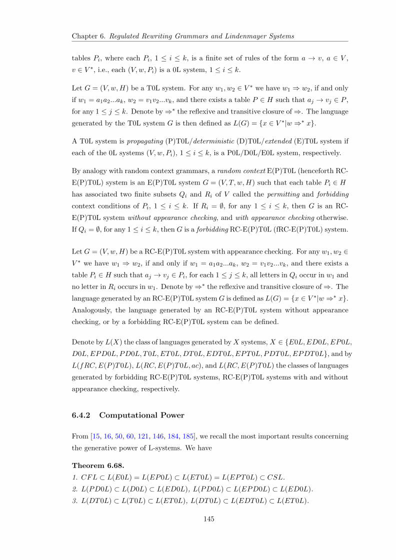
Chapter 6. Regulated Rewriting Grammars and Lindenmayer Systems
tables Pi, where each Pi, 1 ≤ i ≤ k, is a finite set of rules of the form a → v, a ∈ V ,
v ∈ V ∗, i.e., each (V,w, Pi) is a 0L system, 1 ≤ i ≤ k.
Let G = (V,w,H) be a T0L system. For any w1, w2 ∈ V ∗ we have w1 ⇒ w2, if and only
if w1 = a1a2...ak, w2 = v1v2...vk, and there exists a table P ∈ H such that aj → vj ∈ P ,
for any 1 ≤ j ≤ k. Denote by⇒∗ the reflexive and transitive closure of⇒. The language
generated by the T0L system G is then defined as L(G) = x ∈ V ∗|w ⇒∗ x.
A T0L system is propagating (P)T0L/deterministic (D)T0L/extended (E)T0L system if
each of the 0L systems (V,w, Pi), 1 ≤ i ≤ k, is a P0L/D0L/E0L system, respectively.
By analogy with random context grammars, a random context E(P)T0L (henceforth RC-
E(P)T0L) system is an E(P)T0L system G = (V, T,w,H) such that each table Pi ∈ Hhas associated two finite subsets Qi and Ri of V called the permitting and forbidding
context conditions of Pi, 1 ≤ i ≤ k. If Ri = ∅, for any 1 ≤ i ≤ k, then G is an RC-
E(P)T0L system without appearance checking, and with appearance checking otherwise.
If Qi = ∅, for any 1 ≤ i ≤ k, then G is a forbidding RC-E(P)T0L (fRC-E(P)T0L) system.
Let G = (V,w,H) be a RC-E(P)T0L system with appearance checking. For any w1, w2 ∈V ∗ we have w1 ⇒ w2, if and only if w1 = a1a2...ak, w2 = v1v2...vk, and there exists a
table Pi ∈ H such that aj → vj ∈ Pi, for each 1 ≤ j ≤ k, all letters in Qi occur in w1 and
no letter in Ri occurs in w1. Denote by⇒∗ the reflexive and transitive closure of⇒. The
language generated by an RC-E(P)T0L systemG is defined as L(G) = x ∈ V ∗|w ⇒∗ x.Analogously, the language generated by an RC-E(P)T0L system without appearance
checking, or by a forbidding RC-E(P)T0L system can be defined.
Denote by L(X) the class of languages generated byX systems, X ∈ E0L,ED0L,EP0L,
D0L,EPD0L,PD0L, T0L,ET0L,DT0L,EDT0L,EPT0L,PDT0L,EPDT0L, and by
L(fRC,E(P )T0L), L(RC,E(P )T0L, ac), and L(RC,E(P )T0L) the classes of languages
generated by forbidding RC-E(P)T0L systems, RC-E(P)T0L systems with and without
appearance checking, respectively.
6.4.2 Computational Power
From [15, 16, 50, 60, 121, 146, 184, 185], we recall the most important results concerning
the generative power of L-systems. We have
Theorem 6.68.
1. CFL ⊂ L(E0L) = L(EP0L) ⊂ L(ET0L) = L(EPT0L) ⊂ CSL.
2. L(PD0L) ⊂ L(D0L) ⊂ L(ED0L), L(PD0L) ⊂ L(EPD0L) ⊂ L(ED0L).
3. L(DT0L) ⊂ L(T0L) ⊂ L(ET0L), L(DT0L) ⊂ L(EDT0L) ⊂ L(ET0L).
145
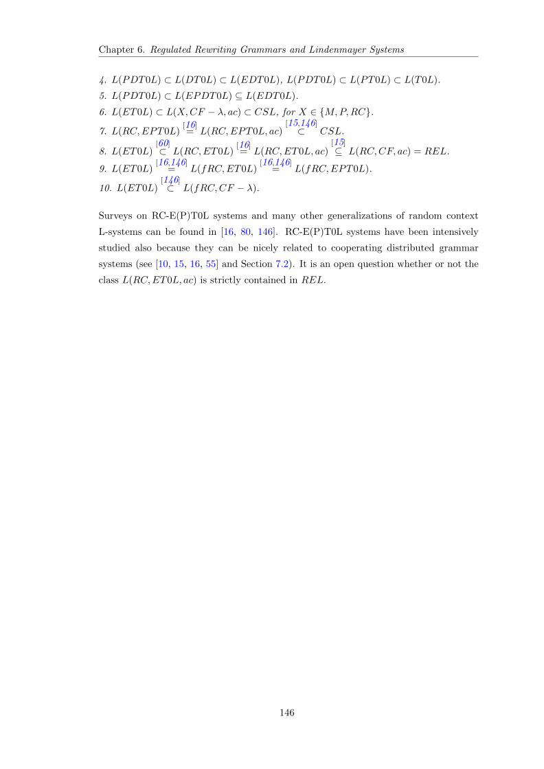
Chapter 6. Regulated Rewriting Grammars and Lindenmayer Systems
4. L(PDT0L) ⊂ L(DT0L) ⊂ L(EDT0L), L(PDT0L) ⊂ L(PT0L) ⊂ L(T0L).
5. L(PDT0L) ⊂ L(EPDT0L) ⊆ L(EDT0L).
6. L(ET0L) ⊂ L(X,CF − λ, ac) ⊂ CSL, for X ∈ M,P,RC.
7. L(RC,EPT0L)[16]= L(RC,EPT0L, ac)
[15,146]⊂ CSL.
8. L(ET0L)[60]⊂ L(RC,ET0L)
[16]= L(RC,ET0L, ac)
[15]
⊆ L(RC,CF, ac) = REL.
9. L(ET0L)[16,146]
= L(fRC,ET0L)[16,146]
= L(fRC,EPT0L).
10. L(ET0L)[146]⊂ L(fRC,CF − λ).
Surveys on RC-E(P)T0L systems and many other generalizations of random context
L-systems can be found in [16, 80, 146]. RC-E(P)T0L systems have been intensively
studied also because they can be nicely related to cooperating distributed grammar
systems (see [10, 15, 16, 55] and Section 7.2). It is an open question whether or not the
class L(RC,ET0L, ac) is strictly contained in REL.
146

Chapter 7
Grammar Systems
What would make theoreticians work-
ing on grammar systems even happier?
To have computer systems that make
use of their models. For instance, to
have a Compiler for a multiprocessor
computer/system - this would naturally
have to be based on a variant of gram-
mar systems. (V. Mihalache, [151])
Grammar systems are a formal model of multiagent systems in cooperative distributed
problem solving, in which the information is distributed to cooperating parts in order
to resolve a problem. Hence, a grammar system is a network of grammars that function
together according to a specified protocol of cooperation. Grammar systems work under
two main modi-operandum. One is based on a parallel, communicating, and distributed
scheme used by all kind of parallel communicating grammar systems. The other one is
based on a sequential, cooperating, and distributed scheme which is used by all types of
cooperating distributed grammar systems.
Informally, in parallel communicating (PC) grammar systems each grammar has its own
axiom and its own working tape. All grammars work simultaneously, in a synchronized
manner. The protocol of cooperation consists in exchanging strings that have been gen-
erated up to the request moment, by the grammar that has been interrogated. The
system combines by excellency parallelism, dynamical communication, and cooperation
done by request through so called query symbols. These query symbols impose restric-
tions in the collaboration protocol, specifying which grammar has to provide its own
data, seen as sequences of strings, to the grammar that asked for the information. The
first component of the system is called the system’s master. Its tape contains, at the end
147
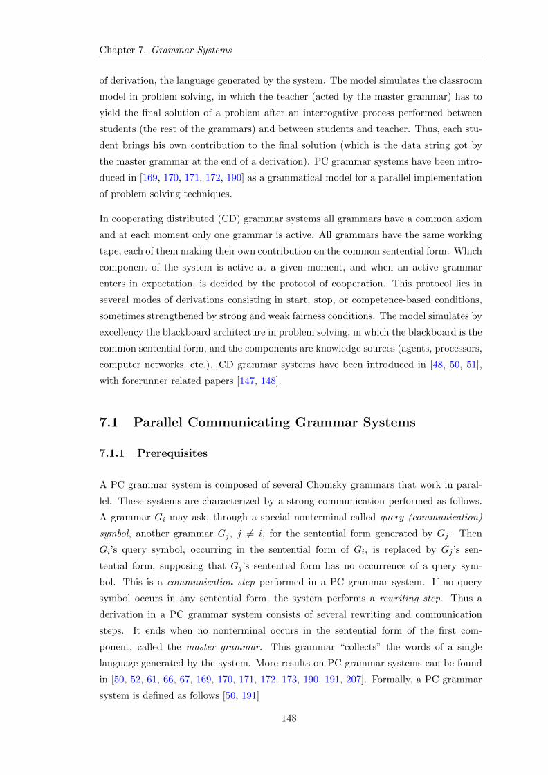
Chapter 7. Grammar Systems
of derivation, the language generated by the system. The model simulates the classroom
model in problem solving, in which the teacher (acted by the master grammar) has to
yield the final solution of a problem after an interrogative process performed between
students (the rest of the grammars) and between students and teacher. Thus, each stu-
dent brings his own contribution to the final solution (which is the data string got by
the master grammar at the end of a derivation). PC grammar systems have been intro-
duced in [169, 170, 171, 172, 190] as a grammatical model for a parallel implementation
of problem solving techniques.
In cooperating distributed (CD) grammar systems all grammars have a common axiom
and at each moment only one grammar is active. All grammars have the same working
tape, each of them making their own contribution on the common sentential form. Which
component of the system is active at a given moment, and when an active grammar
enters in expectation, is decided by the protocol of cooperation. This protocol lies in
several modes of derivations consisting in start, stop, or competence-based conditions,
sometimes strengthened by strong and weak fairness conditions. The model simulates by
excellency the blackboard architecture in problem solving, in which the blackboard is the
common sentential form, and the components are knowledge sources (agents, processors,
computer networks, etc.). CD grammar systems have been introduced in [48, 50, 51],
with forerunner related papers [147, 148].
7.1 Parallel Communicating Grammar Systems
7.1.1 Prerequisites
A PC grammar system is composed of several Chomsky grammars that work in paral-
lel. These systems are characterized by a strong communication performed as follows.
A grammar Gi may ask, through a special nonterminal called query (communication)
symbol, another grammar Gj , j 6= i, for the sentential form generated by Gj . Then
Gi’s query symbol, occurring in the sentential form of Gi, is replaced by Gj ’s sen-
tential form, supposing that Gj ’s sentential form has no occurrence of a query sym-
bol. This is a communication step performed in a PC grammar system. If no query
symbol occurs in any sentential form, the system performs a rewriting step. Thus a
derivation in a PC grammar system consists of several rewriting and communication
steps. It ends when no nonterminal occurs in the sentential form of the first com-
ponent, called the master grammar. This grammar “collects” the words of a single
language generated by the system. More results on PC grammar systems can be found
in [50, 52, 61, 66, 67, 169, 170, 171, 172, 173, 190, 191, 207]. Formally, a PC grammar
system is defined as follows [50, 191]
148
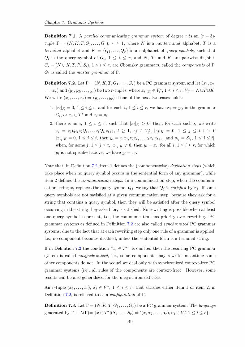
Chapter 7. Grammar Systems
Definition 7.1. A parallel communicating grammar system of degree r is an (r + 3)-
tuple Γ = (N,K, T,G1, . . . , Gr), r ≥ 1, where N is a nonterminal alphabet, T is a
terminal alphabet and K = Q1, . . . , Qr is an alphabet of query symbols, such that
Qi is the query symbol of Gi, 1 ≤ i ≤ r, and N , T , and K are pairwise disjoint.
Gi = (N ∪K,T, Pi, Si), 1 ≤ i ≤ r, are Chomsky grammars, called the components of Γ,
G1 is called the master grammar of Γ.
Definition 7.2. Let Γ = (N,K, T,G1, . . . , Gr) be a PC grammar system and let (x1, x2,
. . . , xr) and (y1, y2, . . . , yr) be two r-tuples, where xi, yi ∈ V ∗Γ , 1 ≤ i ≤ r, VΓ = N∪T∪K.
We write (x1, . . . , xr)⇒ (y1, . . . , yr) if one of the next two cases holds:
1. |xi|K = 0, 1 ≤ i ≤ r, and for each i, 1 ≤ i ≤ r, we have xi ⇒ yi, in the grammar
Gi, or xi ∈ T ∗ and xi = yi;
2. there is an i, 1 ≤ i ≤ r, such that |xi|K > 0; then, for each such i, we write
xi = z1Qi1z2Qi2 . . . ztQitzt+1, t ≥ 1, zj ∈ V ∗Γ , |zj |K = 0, 1 ≤ j ≤ t + 1; if
|xij |K = 0, 1 ≤ j ≤ t, then yi = z1xi1z2xi2 . . . ztxitzt+1 [and yij = Sij , 1 ≤ j ≤ t];
when, for some j, 1 ≤ j ≤ t, |xij |K 6= 0, then yi = xi; for all i, 1 ≤ i ≤ r, for which
yi is not specified above, we have yi = xi.
Note that, in Definition 7.2, item 1 defines the (componentwise) derivation steps (which
take place when no query symbol occurs in the sentential form of any grammar), while
item 2 defines the communication steps. In a communication step, when the communi-
cation string xj replaces the query symbol Qj , we say that Qj is satisfied by xj . If some
query symbols are not satisfied at a given communication step, because they ask for a
string that contains a query symbol, then they will be satisfied after the query symbol
occurring in the string they asked for, is satisfied. No rewriting is possible when at least
one query symbol is present, i.e., the communication has priority over rewriting. PC
grammar systems as defined in Definition 7.2 are also called synchronized PC grammar
systems, due to the fact that at each rewriting step only one rule of a grammar is applied,
i.e., no component becomes disabled, unless the sentential form is a terminal string.
If in Definition 7.2 the condition “xi ∈ T ∗” is omitted then the resulting PC grammar
system is called unsynchronized, i.e., some components may rewrite, meantime some
other components do not. In the sequel we deal only with synchronized context-free PC
grammar systems (i.e., all rules of the components are context-free). However, some
results can be also generalized for the unsynchronized case.
An r-tuple (x1, . . . , xr), xi ∈ V ∗Γ , 1 ≤ i ≤ r, that satisfies either item 1 or item 2, in
Definition 7.2, is referred to as a configuration of Γ.
Definition 7.3. Let Γ = (N,K, T,G1, . . . , Gr) be a PC grammar system. The language
generated by Γ is L(Γ)= x ∈ T ∗|(S1, . . . , Sr)⇒∗(x, α2, . . . , αr), αi ∈ V ∗Γ , 2 ≤ i ≤ r.
149
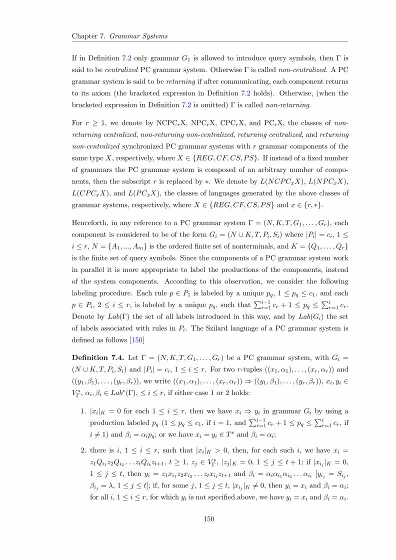
Chapter 7. Grammar Systems
If in Definition 7.2 only grammar G1 is allowed to introduce query symbols, then Γ is
said to be centralized PC grammar system. Otherwise Γ is called non-centralized. A PC
grammar system is said to be returning if after communicating, each component returns
to its axiom (the bracketed expression in Definition 7.2 holds). Otherwise, (when the
bracketed expression in Definition 7.2 is omitted) Γ is called non-returning.
For r ≥ 1, we denote by NCPCrX, NPCrX, CPCrX, and PCrX, the classes of non-
returning centralized, non-returning non-centralized, returning centralized, and returning
non-centralized synchronized PC grammar systems with r grammar components of the
same type X, respectively, where X ∈ REG,CF,CS, PS. If instead of a fixed number
of grammars the PC grammar system is composed of an arbitrary number of compo-
nents, then the subscript r is replaced by ∗. We denote by L(NCPCxX), L(NPCxX),
L(CPCxX), and L(PCxX), the classes of languages generated by the above classes of
grammar systems, respectively, where X ∈ REG,CF,CS, PS and x ∈ r, ∗.
Henceforth, in any reference to a PC grammar system Γ = (N,K, T,G1, . . . , Gr), each
component is considered to be of the form Gi = (N ∪K,T, Pi, Si) where |Pi| = ci, 1 ≤i ≤ r, N = A1, ..., Am is the ordered finite set of nonterminals, and K = Q1, . . . , Qris the finite set of query symbols. Since the components of a PC grammar system work
in parallel it is more appropriate to label the productions of the components, instead
of the system components. According to this observation, we consider the following
labeling procedure. Each rule p ∈ P1 is labeled by a unique pq, 1 ≤ pq ≤ c1, and each
p ∈ Pi, 2 ≤ i ≤ r, is labeled by a unique pq, such that∑i−1
r=1 cr + 1 ≤ pq ≤∑i
r=1 cr.
Denote by Lab(Γ) the set of all labels introduced in this way, and by Lab(Gi) the set
of labels associated with rules in Pi. The Szilard language of a PC grammar system is
defined as follows [150]
Definition 7.4. Let Γ = (N,K, T,G1, . . . , Gr) be a PC grammar system, with Gi =
(N ∪K,T, Pi, Si) and |Pi| = ci, 1 ≤ i ≤ r. For two r-tuples ((x1, α1), . . . , (xr, αr)) and
((y1, β1), . . . , (yr, βr)), we write ((x1, α1), . . . , (xr, αr)) ⇒ ((y1, β1), . . . , (yr, βr)), xi, yi ∈V ∗Γ , αi, βi ∈ Lab∗(Γ), ≤ i ≤ r, if either case 1 or 2 holds:
1. |xi|K = 0 for each 1 ≤ i ≤ r, then we have xi ⇒ yi in grammar Gi by using a
production labeled pq (1 ≤ pq ≤ c1, if i = 1, and∑i−1
r=1 cr + 1 ≤ pq ≤∑i
r=1 cr, if
i 6= 1) and βi = αipq; or we have xi = yi ∈ T ∗ and βi = αi;
2. there is i, 1 ≤ i ≤ r, such that |xi|K > 0, then, for each such i, we have xi =
z1Qi1z2Qi2 . . . ztQitzt+1, t ≥ 1, zj ∈ V ∗Γ , |zj |K = 0, 1 ≤ j ≤ t + 1; if |xij |K = 0,
1 ≤ j ≤ t, then yi = z1xi1z2xi2 . . . ztxitzt+1 and βi = αiαi1αi2 . . . αit [yij = Sij ,
βij = λ, 1 ≤ j ≤ t]; if, for some j, 1 ≤ j ≤ t, |xij |K 6= 0, then yi = xi and βi = αi;
for all i, 1 ≤ i ≤ r, for which yi is not specified above, we have yi = xi and βi = αi.
150
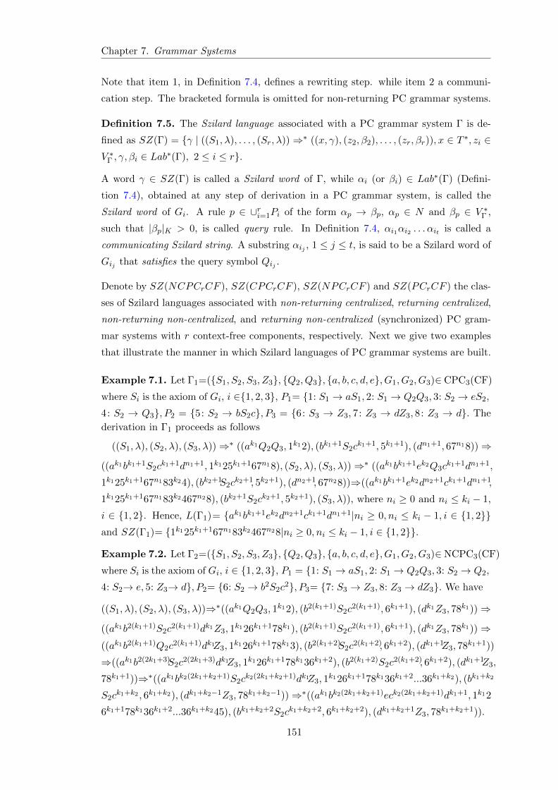
Chapter 7. Grammar Systems
Note that item 1, in Definition 7.4, defines a rewriting step. while item 2 a communi-
cation step. The bracketed formula is omitted for non-returning PC grammar systems.
Definition 7.5. The Szilard language associated with a PC grammar system Γ is de-
fined as SZ(Γ) = γ | ((S1, λ), . . . , (Sr, λ))⇒∗ ((x, γ), (z2, β2), . . . , (zr, βr)), x ∈ T ∗, zi ∈V ∗Γ , γ, βi ∈ Lab∗(Γ), 2 ≤ i ≤ r.
A word γ ∈ SZ(Γ) is called a Szilard word of Γ, while αi (or βi) ∈ Lab∗(Γ) (Defini-
tion 7.4), obtained at any step of derivation in a PC grammar system, is called the
Szilard word of Gi. A rule p ∈ ∪ri=1Pi of the form αp → βp, αp ∈ N and βp ∈ V ∗Γ ,
such that |βp|K > 0, is called query rule. In Definition 7.4, αi1αi2 . . . αit is called a
communicating Szilard string. A substring αij , 1 ≤ j ≤ t, is said to be a Szilard word of
Gij that satisfies the query symbol Qij .
Denote by SZ(NCPCrCF ), SZ(CPCrCF ), SZ(NPCrCF ) and SZ(PCrCF ) the clas-
ses of Szilard languages associated with non-returning centralized, returning centralized,
non-returning non-centralized, and returning non-centralized (synchronized) PC gram-
mar systems with r context-free components, respectively. Next we give two examples
that illustrate the manner in which Szilard languages of PC grammar systems are built.
Example 7.1. Let Γ1=(S1, S2, S3, Z3, Q2, Q3, a, b, c, d, e, G1, G2, G3)∈ CPC3(CF)
where Si is the axiom of Gi, i ∈1, 2, 3, P1= 1: S1 → aS1, 2: S1 → Q2Q3, 3: S2 → eS2,
4: S2 → Q3, P2 = 5: S2 → bS2c, P3 = 6: S3 → Z3, 7: Z3 → dZ3, 8: Z3 → d. The
derivation in Γ1 proceeds as follows
((S1, λ), (S2, λ), (S3, λ))⇒∗ ((ak1Q2Q3, 1k12), (bk1+1S2c
k1+1, 5k1+1), (dn1+1, 67n18))⇒
((ak1bk1+1S2ck1+1dn1+1, 1k125k1+167n18), (S2, λ), (S3, λ))⇒∗ ((ak1bk1+1ek2Q3c
k1+1dn1+1,
1k125k1+167n183k24), (bk2+1S2ck2+1, 5k2+1), (dn2+1, 67n28))⇒((ak1bk1+1ek2dn2+1ck1+1dn1+1,
1k125k1+167n183k2467n28), (bk2+1S2ck2+1, 5k2+1), (S3, λ)), where ni ≥ 0 and ni ≤ ki − 1,
i ∈ 1, 2. Hence, L(Γ1)= ak1bk1+1ek2dn2+1ck1+1dn1+1|ni ≥ 0, ni ≤ ki − 1, i ∈ 1, 2and SZ(Γ1)= 1k125k1+167n183k2467n28|ni ≥ 0, ni ≤ ki − 1, i ∈ 1, 2.
Example 7.2. Let Γ2=(S1, S2, S3, Z3, Q2, Q3, a, b, c, d, e, G1, G2, G3)∈NCPC3(CF)
where Si is the axiom of Gi, i ∈ 1, 2, 3, P1 = 1: S1 → aS1, 2: S1 → Q2Q3, 3: S2 → Q2,
4: S2→ e, 5: Z3→ d, P2= 6: S2 → b2S2c2, P3= 7: S3 → Z3, 8: Z3 → dZ3. We have
((S1, λ), (S2, λ), (S3, λ))⇒∗((ak1Q2Q3, 1k12), (b2(k1+1)S2c
2(k1+1), 6k1+1), (dk1Z3, 78k1))⇒
((ak1b2(k1+1)S2c2(k1+1)dk1Z3, 1
k126k1+178k1), (b2(k1+1)S2c2(k1+1), 6k1+1), (dk1Z3, 78k1))⇒
((ak1b2(k1+1)Q2c2(k1+1)dk1Z3, 1
k126k1+178k13), (b2(k1+2)S2c2(k1+2), 6k1+2), (dk1+1Z3, 78k1+1))
⇒((ak1b2(2k1+3)S2c2(2k1+3)dk1Z3, 1
k126k1+178k136k1+2), (b2(k1+2)S2c2(k1+2), 6k1+2), (dk1+1Z3,
78k1+1))⇒∗((ak1bk2(2k1+k2+1)S2ck2(2k1+k2+1)dk1Z3, 1
k126k1+178k136k1+2...36k1+k2), (bk1+k2
S2ck1+k2 , 6k1+k2), (dk1+k2−1Z3, 78k1+k2−1))⇒∗((ak1bk2(2k1+k2+1)eck2(2k1+k2+1)dk1+1, 1k12
6k1+178k136k1+2...36k1+k245), (bk1+k2+2S2ck1+k2+2, 6k1+k2+2), (dk1+k2+1Z3, 78k1+k2+1)).
151
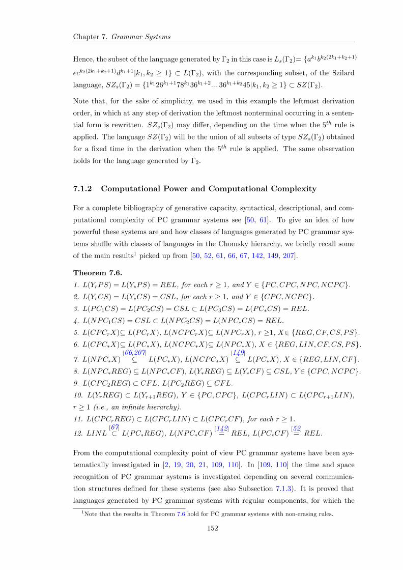
Chapter 7. Grammar Systems
Hence, the subset of the language generated by Γ2 in this case is Ls(Γ2)= ak1bk2(2k1+k2+1)
eck2(2k1+k2+1)dk1+1|k1, k2 ≥ 1 ⊂ L(Γ2), with the corresponding subset, of the Szilard
language, SZs(Γ2) = 1k126k1+178k136k1+2... 36k1+k245|k1, k2 ≥ 1 ⊂ SZ(Γ2).
Note that, for the sake of simplicity, we used in this example the leftmost derivation
order, in which at any step of derivation the leftmost nonterminal occurring in a senten-
tial form is rewritten. SZs(Γ2) may differ, depending on the time when the 5th rule is
applied. The language SZ(Γ2) will be the union of all subsets of type SZs(Γ2) obtained
for a fixed time in the derivation when the 5th rule is applied. The same observation
holds for the language generated by Γ2.
7.1.2 Computational Power and Computational Complexity
For a complete bibliography of generative capacity, syntactical, descriptional, and com-
putational complexity of PC grammar systems see [50, 61]. To give an idea of how
powerful these systems are and how classes of languages generated by PC grammar sys-
tems shuffle with classes of languages in the Chomsky hierarchy, we briefly recall some
of the main results1 picked up from [50, 52, 61, 66, 67, 142, 149, 207].
Theorem 7.6.
1. L(YrPS) = L(Y∗PS) = REL, for each r ≥ 1, and Y ∈ PC,CPC,NPC,NCPC.2. L(YrCS) = L(Y∗CS) = CSL, for each r ≥ 1, and Y ∈ CPC,NCPC.3. L(PC1CS) = L(PC2CS) = CSL ⊂ L(PC3CS) = L(PC∗CS) = REL.
4. L(NPC1CS) = CSL ⊂ L(NPC2CS) = L(NPC∗CS) = REL.
5. L(CPCrX)⊆ L(PCrX), L(NCPCrX)⊆ L(NPCrX), r ≥1, X∈ REG,CF,CS, PS.6. L(CPC∗X)⊆ L(PC∗X), L(NCPC∗X)⊆ L(NPC∗X), X ∈ REG,LIN,CF,CS, PS.
7. L(NPC∗X)[66,207]
⊆ L(PC∗X), L(NCPC∗X)[149]
⊆ L(PC∗X), X ∈ REG,LIN,CF.8. L(NPC∗REG) ⊆ L(NPC∗CF ), L(Y∗REG) ⊆ L(Y∗CF ) ⊆ CSL, Y ∈ CPC,NCPC.9. L(CPC2REG) ⊂ CFL, L(PC2REG) ⊆ CFL.
10. L(YrREG) ⊂ L(Yr+1REG), Y ∈ PC,CPC, L(CPCrLIN) ⊂ L(CPCr+1LIN),
r ≥ 1 (i.e., an infinite hierarchy).
11. L(CPCrREG) ⊂ L(CPCrLIN) ⊂ L(CPCrCF ), for each r ≥ 1.
12. LINL[67]⊂ L(PC∗REG), L(NPC∗CF )
[142]= REL, L(PC∗CF )
[52]= REL.
From the computational complexity point of view PC grammar systems have been sys-
tematically investigated in [2, 19, 20, 21, 109, 110]. In [109, 110] the time and space
recognition of PC grammar systems is investigated depending on several communica-
tion structures defined for these systems (see also Subsection 7.1.3). It is proved that
languages generated by PC grammar systems with regular components, for which the
1Note that the results in Theorem 7.6 hold for PC grammar systems with non-erasing rules.
152
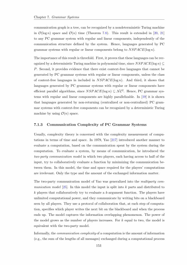
Chapter 7. Grammar Systems
communication graph is a tree, can be recognized by a nondeterministic Turing machine
in O(log n) space and O(n) time (Theorem 7.8). This result is extended in [20, 21]
to any PC grammar system with regular and linear components, independently of the
communication structure defined by the system. Hence, languages generated by PC
grammar systems with regular or linear components belong to NSPACE(log n).
The importance of this result is threefold. First, it proves that these languages can be rec-
ognized by a deterministic Turing machine in polynomial time, since NSPACE(log n) ⊆P . Second, it provides evidence that there exist context-free languages that cannot be
generated by PC grammar systems with regular or linear components, unless the class
of context-free languages in included in NSPACE(log n). And third, it shows that
languages generated by PC grammar systems with regular or linear components have
efficient parallel algorithms, since NSPACE(log n) ⊆ NC2. Hence, PC grammar sys-
tems with regular and linear components are highly parallelizable. In [19] it is shown
that languages generated by non-returning (centralized or non-centralized) PC gram-
mar systems with context-free components can be recognized by a deterministic Turing
machine by using O(n) space.
7.1.3 Communication Complexity of PC Grammar Systems
Usually, complexity theory is concerned with the complexity measurement of compu-
tations in terms of time and space. In 1979, Yao [217] introduced another manner to
evaluate a computation, based on the communication spent by the system during the
computation. To evaluate a system, by means of communication, he introduced the
two-party communication model in which two players, each having access to half of the
input, try to collaboratively evaluate a function by minimizing the communication be-
tween them. In this model, the time and space required for the players’ computations
are irrelevant. Only the type and the amount of the exchanged information matter.
The two-party communication model of Yao was generalized into the multiparty com-
munication model [25]. In this model the input is split into k parts and distributed to
k players that collaboratively try to evaluate a k-argument function. The players have
unlimited computational power, and they communicate by writing bits on a blackboard
seen by all players. They use a protocol of collaboration that, at each step of computa-
tion, specifies which player writes the next bit on the blackboard and when the process
ends up. The model captures the information overlapping phenomenon. The power of
the model grows as the number of players increases. For k equal to two, the model is
equivalent with the two-party model.
Informally, the communication complexity of a computation is the amount of information
(e.g., the sum of the lengths of all messages) exchanged during a computational process
153
Chapter 7. Grammar Systems
between parts of the system that supports the computation. Communication complexity
has been identified as an interesting tool for proving lower bounds in the study of small
complexity classes.
PC grammar systems are an attracting topic not only because of their composite struc-
ture and cooperating/distribuited manner in which the derivation evolves in a parallel
fashion, but also because of the very complex communication strategy used by these sys-
tems, which remembers about the inter-processors communication and the multiparty
communication model. This is the main reason why the investigation of the communi-
cation complexity of these systems was an unavoidable issue.
To achieve the communication complexity in PC grammar systems two communication
complexity measures have been proved to be illustrative for them [109, 110, 165, 166].
The first measure, introduced in [109, 110], is the communication structure of a PC
grammar system. This is the shape of the communication graph consisting of directed
communication links between the grammars. The second measure, introduced in [110,
165], is the communication complexity of a PC grammar system, and it represents the
number of messages (communications) exchanged, during the derivation of a certain
word, between the system’s components. This is a function of the length of the generated
word. Hence, it is a computational complexity measure.
The communication graph of a PC grammar system [109, 110] is a directed graph in
which the vertices are labeled by the system’s grammars and the edges are oriented
from the grammar that contains on its sentential form a query symbol, to the grammar
to which the query symbol belongs. If Γ is a PC grammar system, then a dag-PCGS, tree-
PCGS, two-way array-PCGS, one-way array-PCGS, two-way ring-PCGS, one-way ring-
PCGS (cycle) is a PC grammar system whose communication graph is a directed acyclic
graph, tree, two-way array, one-way array, two-way ring, one-way ring (cycle), respec-
tively. Denote by Π(Γ) the communication graph associated to Γ. Let x-PCGSr be the
class of PC grammar systems of degree r whose communication graph is of type x, where2
x ∈ c, dag, tree, two-way-array, one-way-array, two-way-ring, one-way-ring(cycle).
Denote by L(x-PCGSr) the family of languages generated by x−PCGSr’s whose com-
munication graph is of type x, and by x-PCGSr(f(n)) the class of PC grammar systems
having a communication graph of type x, that use at most f(n) communication steps to
generate words of length n, and by L(x-PCGSr(f(n))) the family of languages generated
by PC grammar systems in x-PCGSr(f(n)). From [109] we have the next characteriza-
tion of tree-PCGS by means of multicounter machines (Definition 4.11).
2Here, c stands for centralized. A ring (or cycle) is a graph in which each vertex connects exactly twoother vertices. An array is a ring in which one of the edges is deleted.
154
Chapter 7. Grammar Systems
Lemma 7.7. Let Γ be a tree-PCGS(f(n)) of degree m. For some positive integer m
and for some function f : N → N, there exists a linear-time nondeterministic (m − 1)-
multicounter automaton M , recognizing L(Γ) with 2f(n) reversals and f(n) zero-tests.
Tree-PCGSs and dag-PCGSs can be simulated by off-line multitape Turing machines in
linear time, while the former class by using only logarithmic space. Formally we have
Theorem 7.8. L(tree-PCGS) ⊆ NTIME(n) ∩NSPACE(log n).
Theorem 7.9. L(dag-PCGS) ⊆ NTIME(n).
Since for the case of centralized PC grammar systems (c-PCGSs), returning or not retur-
ning, the communication graph is a star-tree (an one-level tree composed of the master
grammar labeling the root and the other grammars labeling its children) we have
Theorem 7.10. For any f : N → N, f(n) 6∈ Ω(n), and any m, k ∈ N, m ≥ 2, k ≥ 1,
the next relations hold
1. L(c-PCGS2(n))−⋃m∈N L(tree-PCGSm(f(n))) 6= ∅,
2. L(c-PCGSk+1(k))−⋃m∈N L(tree-PCGSm(k − 1)) 6= ∅,
3. L(one-way-array-PCGSm(f(n))) ⊂ L(one-way-array-PCGSm(n)),
4. L(c-PCGSm(f(n))) ⊂ L(c-PCGSm(n)),
5. L(tree-PCGSm(f(n))) ⊂ L(tree-PCGSm(n)),
6. L(X-PCGSk+1(k − 1)) ⊂ L(X-PCGSk+1(k)), X ∈ c, tree, one-way-array,7.⋃m∈N L(X-PCGSm(k−1))⊂
⋃m∈N L(X-PCGSm(k)), X∈c, tree, one-way-array.
Sketch of proof 1. The first claim is true, due to the existence of the language L =
ai1bi1ai2bi2 ...aikbikc|k ≥ 1, ij ∈ N, for j ∈ 1, ..., k ∈ L(c-PCGS2(n))−⋃m∈N L(tree-
PCGSm(f(n))). The second claim is true due to the existence of the language Lk =
ai1bi1ai2bi2 ...aikbi1+i2+...+ikc|k ≥ 1, ij ∈ N, for j ∈ 1, ..., k ∈ L(c-PCGSk+1(k)) −⋃m∈N L(tree-PCGSm(k − 1)). Items 3 - 5 are direct consequences of 1, while 6 and 7
are consequences of 2.
From [109] we recall the following pumping lemma for dag-PCGSs.
Lemma 7.11. Let L be a language generated by a dag-PCGS of degree r > 1. There
exists a natural number N such that every word α ∈ L whose length is at least N can be
decomposed as α = α1β1α2β2...αmβmαm+1, where βi 6= λ for every i, 1 ≤ i ≤ m, and
1≤ |β1, ..., βm|≤ n. Moreover, for all s ≥ 0, the word α1βs1α2β
s2...αmβ
smαm+1 is in L.
As a consequence of this pumping lemma we have
Theorem 7.12. L(tree-PCGSr)− L(dag-PCGSr−1) 6= ∅, for all r ≥ 1.
155
Chapter 7. Grammar Systems
Proof. Consider the language Lr = ak+11 ak+2
2 ...ak+rr |k ≥ 0, which can be generated by
the following tree-PCGS Γ = (N,K, T, (P1, S1), . . . , (Pr, Sr)), where
T = a1, a2, ..., ar, N = S1, S2, ..., Sr, K = Q1, Q2, ..., Qr,P1 = S1 −→ a1S1, Sr −→ ar ∪ Si −→ aiQi+1|1 ≤ i ≤ r − 1,Pi = Si −→ aiSi, 2 ≤ i ≤ r.
The above language cannot be generated by a dag-PCGS, of degree r− 1 or smaller. To
derive a contradiction, let N be the natural number provided by Lemma 7.11 and α ∈ Lrof the form α = aN+1
1 aN+22 ...aN+r
r . Then the word α(s), obtained from α by pumping at
most r − 1 different subwords of it belongs to Lr, too. On the other hand, the pumped
subwords are in the set A = aki |1 ≤ i ≤ r, of which cardinality is r. Hence, pumping
only r−1 different strings belonging to A, and omitting, let say the string akl , for a fixed
l, the exponent of al in the resulting string remain bounded, while the exponents of the
other ai, i 6= l, grow arbitrarily large. Hence, α(s) /∈ Lr, which leads to a contradiction.
Thus Lr ∈ L(tree-PCGSr)− L(dag-PCGSr−1).
The following infinite hierarchies are consequences of the above theorem.
Corollary 7.13. For all r ≥ 1,
1. L(dag-PCGSr)−L(dag-PCGSr−1) 6= ∅ (hierarchy L(dag-PCGSr)r≥1 is infinite),
2. L(tree-PCGSr)−L(tree-PCGSr−1) 6= ∅ (hierarchy L(tree-PCGSr)r≥1 is infinite).
Theorem 7.14. For all r ≥ 1, L(x-PCGSr+1)−L(x-PCGSr) 6= ∅, where x ∈ two-way-
array, two-way-ring, one-way-ring.
As a consequence of Theorem 7.14 we have
Corollary 7.15. The hierarchies L(x-PCGSr)r≥1, where x ∈ two-way-array, two-
way-ring, one-way-ring are infinite.
Related to the Chomsky hierarchy, from [109, 110], we have the following result
Theorem 7.16. Let Γ be a PC grammar system and Π(Γ) the associated communicating
graph. If the following properties hold:
1. Π(Γ) contains at most one cycle,
2. Π(Γ) contains a cycle, then this cycle involves the master grammar G1,
3. Π(Γ) generates a language over one-letter alphabet.
Then L(Γ) is a regular language.
Corollary 7.17. Let Γ ∈ x-PCGS, x ∈ cycle, dag, generating a language over one
letter alphabet. Then L(Γ) is a regular language.
With respect to the communication complexity measure, in [109, 165], several class hi-
erarchies are obtained along with several lower-bound results. In [165] it is proved that
156
Chapter 7. Grammar Systems
k + 1 communications are more powerful than k communications, independently of the
length of the generated word. This is because, for any natural number k ≥ 1, there
exists a language, e.g., Lk = ai1bi1ai2bi1+i2 ... aikbi1+i2+...+ik |ij ∈ N, which can be gen-
erated by a PC grammar system with k communications, but it cannot be generated
by any PC grammar system using k − 1 communications. Hence, there exists an infi-
nite hierarchy of constant communication complexity for PC grammar systems without
restrictions on their communication graphs. There exists also an infinite hierarchy of
O( k√n) communication complexity, k ≥ 2.
Furthermore, every language over one-letter alphabet generated by a PC grammar sys-
tem using constant communication complexity, is regular. The price to obtain non-
regular languages over one letter alphabet is Ω(log n) communication complexity. In
[165] it is proved that, if the communication cannot be bounded by any constant then
it is at least Ω(log n), hence there is a gap between O(1) and Ω(log n) communication
complexity. On the other hand, Ω(log n) is a sufficient and necessary condition to ob-
tain nonregular languages that cannot be generated by using constant communication
complexity. Therefore, this is a lower bound communication complexity for nonregular
languages. A similar result is found in [109], where it is proved that the communication
complexity of dag-PCGSs is either a constant or a linear function. Hence there is a
gap between O(1) and O(n) communication complexity for PC grammar systems whose
communication graph is a dag.
7.1.4 Complexity Results for Szilard Languages of PC Grammar
Systems
The notion of Szilard language (Definition 7.5) of a PC grammar system was introduced
in [150] in order to keep control of derivations in PC grammar systems and to measure
the amount of work, cooperation, and communication performed by the components of
the system. The main objective in [150] was to study properties and relations between
classes of Szilard languages associated with several kind of PC grammar systems. Below
we recall, from [150], only some of the most important results for our considerations.
Theorem 7.18. For any class Y of grammars and any r ≥ 1 we have
1. SZ(CPCrY ) ⊆ SZ(PCrY ), SZ(NCPCrY ) ⊆ SZ(NPCrY ),
2. SZ(XrY ) ⊆ SZ(Xr+1Y ), for any X ∈ CPC,NPC,NCPC,PC.3. SZ(XrY1) ⊆ SZ(XrY2), for any X ∈ CPC,NPC,NCPC,PC, and any Y1, Y2 ∈REG,LIN,CF such that L(Y1) ⊆ L(Y2).
4. REG ⊂ SZ(CPC2REG) ⊂ CFL, SZ(PC2REG) ⊆ CFL.
5. SZ(XrREG) ⊆ L(XrREG), X ∈ CPC,NPC,NCPC,PC.
157
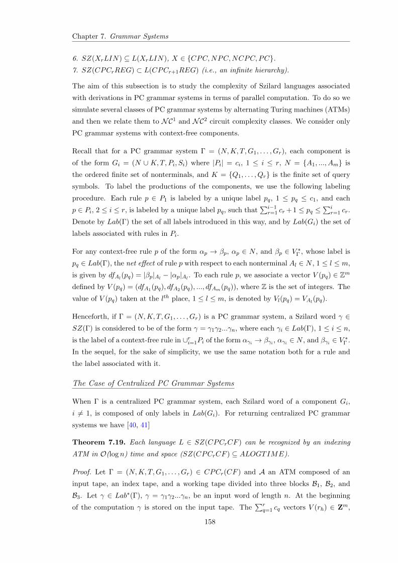
Chapter 7. Grammar Systems
6. SZ(XrLIN) ⊆ L(XrLIN), X ∈ CPC,NPC,NCPC,PC.7. SZ(CPCrREG) ⊂ L(CPCr+1REG) (i.e., an infinite hierarchy).
The aim of this subsection is to study the complexity of Szilard languages associated
with derivations in PC grammar systems in terms of parallel computation. To do so we
simulate several classes of PC grammar systems by alternating Turing machines (ATMs)
and then we relate them to NC1 and NC2 circuit complexity classes. We consider only
PC grammar systems with context-free components.
Recall that for a PC grammar system Γ = (N,K, T,G1, . . . , Gr), each component is
of the form Gi = (N ∪ K,T, Pi, Si) where |Pi| = ci, 1 ≤ i ≤ r, N = A1, ..., Am is
the ordered finite set of nonterminals, and K = Q1, . . . , Qr is the finite set of query
symbols. To label the productions of the components, we use the following labeling
procedure. Each rule p ∈ P1 is labeled by a unique label pq, 1 ≤ pq ≤ c1, and each
p ∈ Pi, 2 ≤ i ≤ r, is labeled by a unique label pq, such that∑i−1
r=1 cr + 1 ≤ pq ≤∑i
r=1 cr.
Denote by Lab(Γ) the set of all labels introduced in this way, and by Lab(Gi) the set of
labels associated with rules in Pi.
For any context-free rule p of the form αp → βp, αp ∈ N , and βp ∈ V ∗Γ , whose label is
pq ∈ Lab(Γ), the net effect of rule p with respect to each nonterminal Al ∈ N , 1 ≤ l ≤ m,
is given by dfAl(pq) = |βp|Al − |αp|Al . To each rule p, we associate a vector V (pq) ∈ Zm
defined by V (pq) = (dfA1(pq), dfA2(pq), ..., dfAm(pq)), where Z is the set of integers. The
value of V (pq) taken at the lth place, 1 ≤ l ≤ m, is denoted by Vl(pq) = VAl(pq).
Henceforth, if Γ = (N,K, T,G1, . . . , Gr) is a PC grammar system, a Szilard word γ ∈SZ(Γ) is considered to be of the form γ = γ1γ2...γn, where each γi ∈ Lab(Γ), 1 ≤ i ≤ n,
is the label of a context-free rule in ∪ri=1Pi of the form αγi → βγi , αγi ∈ N , and βγi ∈ V ∗Γ .
In the sequel, for the sake of simplicity, we use the same notation both for a rule and
the label associated with it.
The Case of Centralized PC Grammar Systems
When Γ is a centralized PC grammar system, each Szilard word of a component Gi,
i 6= 1, is composed of only labels in Lab(Gi). For returning centralized PC grammar
systems we have [40, 41]
Theorem 7.19. Each language L ∈ SZ(CPCrCF ) can be recognized by an indexing
ATM in O(log n) time and space (SZ(CPCrCF ) ⊆ ALOGTIME).
Proof. Let Γ = (N,K, T,G1, . . . , Gr) ∈ CPCr(CF ) and A an ATM composed of an
input tape, an index tape, and a working tape divided into three blocks B1, B2, and
B3. Let γ ∈ Lab∗(Γ), γ = γ1γ2...γn, be an input word of length n. At the beginning
of the computation γ is stored on the input tape. The∑r
q=1 cq vectors V (rh) ∈ Zm,
158
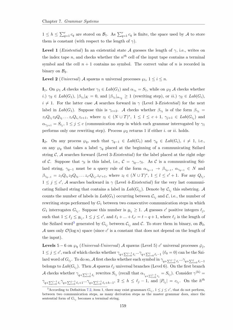
Chapter 7. Grammar Systems
1 ≤ h ≤∑r
q=1 cq are stored on B1. As∑r
q=1 cq is finite, the space used by A to store
them is constant (with respect to the length of γ).
Level 1 (Existential) In an existential state A guesses the length of γ, i.e., writes on
the index tape n, and checks whether the nth cell of the input tape contains a terminal
symbol and the cell n + 1 contains no symbol. The correct value of n is recorded in
binary on B2.
Level 2 (Universal) A spawns n universal processes ℘i, 1 ≤ i ≤ n.
I1. On ℘1 A checks whether γ1 ∈ Lab(G1) and αγ1 = S1, while on ℘2 A checks whether
i.) γ2 ∈ Lab(G1), |βγ1 |K = 0, and |βγ1 |αγ2≥ 1 (rewriting step), or ii.) γ2 ∈ Lab(Gi),
i 6= 1. For the latter case A searches forward in γ (Level 3-Existential) for the next
label in Lab(G1). Suppose this is γc+2. A checks whether βγ1 is of the form βγ1 =
z1Qi1z2Qi2 . . . zcQiczc+1, where zl ∈ (N ∪ T )∗, 1 ≤ l ≤ c + 1, γj+1 ∈ Lab(Gij ) and
αγj+1 = Sij , 1 ≤ j ≤ c (communication step in which each grammar interrogated by γ1
performs only one rewriting step). Process ℘2 returns 1 if either i. or ii. holds.
I2. On any process ℘q, such that γq−1 ∈ Lab(G1) and γq ∈ Lab(Gi), i 6= 1, i.e.,
on any ℘q that takes a label γq placed at the beginning of a communicating Szilard
string C, A searches forward (Level 3-Existential) for the label placed at the right edge
of C. Suppose that γt is this label, i.e., C = γq...γt. As C is a communicating Szi-
lard string, γq−1 must be a query rule of the form αγq−1 → βγq−1 , αγq−1 ∈ N and
βγq−1 = z1Qi1z2Qi2 . . . zc′Qic′zc′+1, where zl ∈ (N ∪ T )∗, 1 ≤ l ≤ c′ + 1. For any Qij ,
1 ≤ j ≤ c′, A searches backward in γ (Level 4-Existential) for the very last communi-
cating Szilard string that contains a label in Lab(Gij ). Denote by Cij this substring. Acounts the number of labels in Lab(G1) occurring between Cij and C, i.e., the number of
rewriting steps performed by G1 between two consecutive communication steps in which
G1 interrogates Gij . Suppose this number is gij ≥ 1. A guesses c′ positive integers `j ,
such that 1 ≤ `j ≤ gij , 1 ≤ j ≤ c′, and `1 + ...+ `c′ = t− q+ 1, where `j is the length of
the Szilard word3 generated by Gij between Cij and C. To store them in binary, on B3,
A uses only O(log n) space (since c′ is a constant that does not depend on the length of
the input).
Levels 5− 6 on ℘q (Universal-Universal) A spawns (Level 5) c′ universal processes ℘j ,
1 ≤ j ≤ c′, each of which checks whether γq+
∑j−1i=0 `i
...γq+
∑ji=0 `i−1
(`0 = 0) can be the Szi-
lard word ofGij . To do so, A first checks whether each symbol in γq+
∑j−1i=0 `i
...γq+
∑ji=0 `i−1
belongs to Lab(Gij ). Then A spawns `j universal branches (Level 6). On the first branch
A checks whether γq+
∑j−1i=0 `i
rewrites Sij (recall that αγq+
∑j−1i=0
`i
= Sij ). Consider γ(h) =
γq+
∑j−1i=0 `i
γq+
∑j−1i=0 `i+1
...γq+
∑j−1i=0 `i+h−1
, 2 ≤ h ≤ `j − 1, and |Pij | = cij . On the hth
3According to Definition 7.2, item 1, there may exist grammars Gij , 1 ≤ j ≤ c′, that do not perform,between two communication steps, as many derivation steps as the master grammar does, since thesentential form of Gij becomes a terminal string.
159
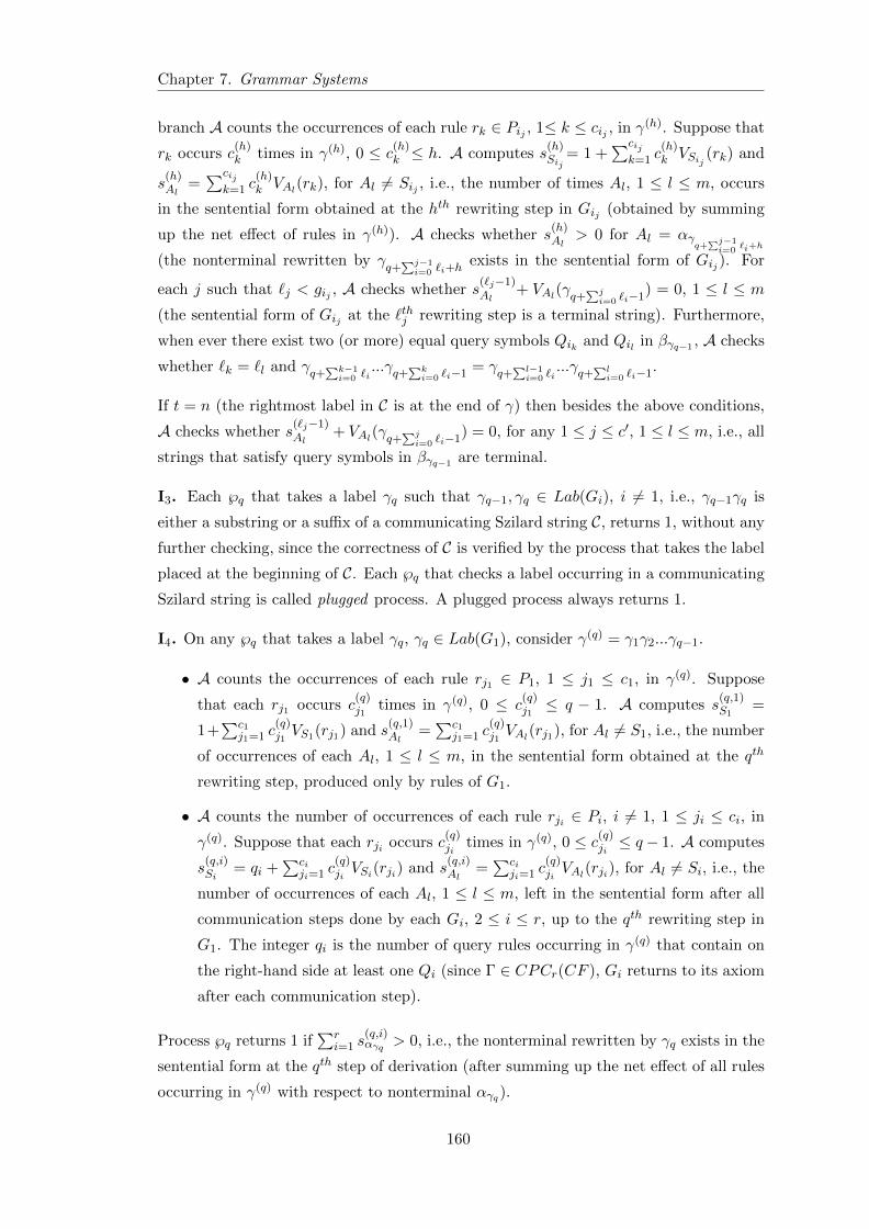
Chapter 7. Grammar Systems
branch A counts the occurrences of each rule rk ∈ Pij , 1≤ k ≤ cij , in γ(h). Suppose that
rk occurs c(h)k times in γ(h), 0 ≤ c
(h)k ≤ h. A computes s
(h)Sij
= 1 +∑cij
k=1 c(h)k VSij (rk) and
s(h)Al
=∑cij
k=1 c(h)k VAl(rk), for Al 6= Sij , i.e., the number of times Al, 1 ≤ l ≤ m, occurs
in the sentential form obtained at the hth rewriting step in Gij (obtained by summing
up the net effect of rules in γ(h)). A checks whether s(h)Al
> 0 for Al = αγq+
∑j−1i=0
`i+h
(the nonterminal rewritten by γq+
∑j−1i=0 `i+h
exists in the sentential form of Gij ). For
each j such that `j < gij , A checks whether s(`j−1)Al
+ VAl(γq+∑ji=0 `i−1
) = 0, 1 ≤ l ≤ m
(the sentential form of Gij at the `thj rewriting step is a terminal string). Furthermore,
when ever there exist two (or more) equal query symbols Qik and Qil in βγq−1 , A checks
whether `k = `l and γq+∑k−1i=0 `i
...γq+∑ki=0 `i−1 = γq+
∑l−1i=0 `i
...γq+∑li=0 `i−1.
If t = n (the rightmost label in C is at the end of γ) then besides the above conditions,
A checks whether s(`j−1)Al
+ VAl(γq+∑ji=0 `i−1
) = 0, for any 1 ≤ j ≤ c′, 1 ≤ l ≤ m, i.e., all
strings that satisfy query symbols in βγq−1 are terminal.
I3. Each ℘q that takes a label γq such that γq−1, γq ∈ Lab(Gi), i 6= 1, i.e., γq−1γq is
either a substring or a suffix of a communicating Szilard string C, returns 1, without any
further checking, since the correctness of C is verified by the process that takes the label
placed at the beginning of C. Each ℘q that checks a label occurring in a communicating
Szilard string is called plugged process. A plugged process always returns 1.
I4. On any ℘q that takes a label γq, γq ∈ Lab(G1), consider γ(q) = γ1γ2...γq−1.
• A counts the occurrences of each rule rj1 ∈ P1, 1 ≤ j1 ≤ c1, in γ(q). Suppose
that each rj1 occurs c(q)j1
times in γ(q), 0 ≤ c(q)j1≤ q − 1. A computes s
(q,1)S1
=
1+∑c1
j1=1 c(q)j1VS1(rj1) and s
(q,1)Al
=∑c1
j1=1 c(q)j1VAl(rj1), for Al 6= S1, i.e., the number
of occurrences of each Al, 1 ≤ l ≤ m, in the sentential form obtained at the qth
rewriting step, produced only by rules of G1.
• A counts the number of occurrences of each rule rji ∈ Pi, i 6= 1, 1 ≤ ji ≤ ci, in
γ(q). Suppose that each rji occurs c(q)ji
times in γ(q), 0 ≤ c(q)ji≤ q− 1. A computes
s(q,i)Si
= qi +∑ci
ji=1 c(q)jiVSi(rji) and s
(q,i)Al
=∑ci
ji=1 c(q)jiVAl(rji), for Al 6= Si, i.e., the
number of occurrences of each Al, 1 ≤ l ≤ m, left in the sentential form after all
communication steps done by each Gi, 2 ≤ i ≤ r, up to the qth rewriting step in
G1. The integer qi is the number of query rules occurring in γ(q) that contain on
the right-hand side at least one Qi (since Γ ∈ CPCr(CF ), Gi returns to its axiom
after each communication step).
Process ℘q returns 1 if∑r
i=1 s(q,i)αγq > 0, i.e., the nonterminal rewritten by γq exists in the
sentential form at the qth step of derivation (after summing up the net effect of all rules
occurring in γ(q) with respect to nonterminal αγq).
160
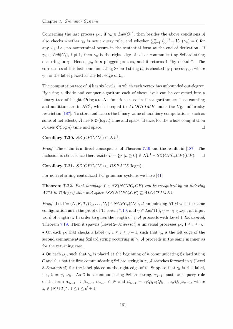
Chapter 7. Grammar Systems
Concerning the last process ℘n, if γn ∈ Lab(G1), then besides the above conditions Aalso checks whether γn is not a query rule, and whether
∑ri=1 s
(n,i)Al
+ VAl(γn) = 0 for
any Al, i.e., no nonterminal occurs in the sentential form at the end of derivation. If
γn ∈ Lab(Gi), i 6= 1, then γn is the right edge of a last communicating Szilard string
occurring in γ. Hence, ℘n is a plugged process, and it returns 1 “by default”. The
correctness of this last communicating Szilard string Cn is checked by process ℘n′ , where
γn′ is the label placed at the left edge of Cn.
The computation tree ofA has six levels, in which each vertex has unbounded out-degree.
By using a divide and conquer algorithm each of these levels can be converted into a
binary tree of height O(log n). All functions used in the algorithm, such as counting
and addition, are in NC1, which is equal to ALOGTIME under the UE∗-uniformity
restriction [187]. To store and access the binary value of auxiliary computations, such as
sums of net effects, A needs O(log n) time and space. Hence, for the whole computation
A uses O(log n) time and space.
Corollary 7.20. SZ(CPCrCF ) ⊂ NC1.
Proof. The claim is a direct consequence of Theorem 7.19 and the results in [187]. The
inclusion is strict since there exists L = pn|n ≥ 0 ∈ NC1 − SZ(CPCrCF )(CF ).
Corollary 7.21. SZ(CPCrCF ) ⊂ DSPACE(log n).
For non-returning centralized PC grammar systems we have [41]
Theorem 7.22. Each language L ∈ SZ(NCPCrCF ) can be recognized by an indexing
ATM in O(log n) time and space (SZ(NCPCrCF ) ⊆ ALOGTIME).
Proof. Let Γ= (N,K, T,G1, . . . , Gr)∈ NCPCr(CF ), A an indexing ATM with the same
configuration as in the proof of Theorem 7.19, and γ ∈ Lab∗(Γ), γ = γ1γ2...γn, an input
word of length n. In order to guess the length of γ, A proceeds with Level 1-Existential,
Theorem 7.19. Then it spawns (Level 2-Universal) n universal processes ℘i, 1 ≤ i ≤ n.
• On each ℘i that checks a label γi, 1 ≤ i ≤ q − 1, such that γq is the left edge of the
second communicating Szilard string occurring in γ, A proceeds in the same manner as
for the returning case.
• On each ℘q, such that γq is placed at the beginning of a communicating Szilard string
C and C is not the first communicating Szilard string in γ, A searches forward in γ (Level
3-Existential) for the label placed at the right edge of C. Suppose that γt is this label,
i.e., C = γq...γt. As C is a communicating Szilard string, γq−1 must be a query rule
of the form αγq−1 → βγq−1 , αγq−1 ∈ N and βγq−1 = z1Qi1z2Qi2 . . . zc′Qic′zc′+1, where
zl ∈ (N ∪ T )∗, 1 ≤ l ≤ c′ + 1.
161
Chapter 7. Grammar Systems
For any symbol Qij occurring in βγq−1 , A searches backward in γ (Level 4-Existential),
for the very last communicating Szilard string that contains a label in Lab(Gij ). Denote
by Cij this communicating Szilard string. A localizes in Cij the Szilard word of Gij that
satisfies Qij . Denote by Sij this Szilard word and by sij the length of Sij (computable
knowing the start and end position of Sij in Cij ). A counts the number of labels in
Lab(G1) occurring between the right edge of Cij and the left edge of C, i.e., the number
of rewriting steps performed by G1 between Cij and C. Suppose this number is gij ≥ 1.
With this information, i.e., sij and gij , acquired for each query symbol in βγq−1 , A guesses
c′ positive integers `j such that sij ≤ `j ≤ sij +gij , 1 ≤ j ≤ c′, and `1 + ...+`j = t−q+1
(each `j is the length of the Szilard word generated by Gij up to C, which is composed
of sij labels in Lab(Gij ) produced up to Cij and gij labels produced between Cij and C).A stores the binary value of sij , gij , and `j , along with the start and end positions of
Sij in γ, 1 ≤ j ≤ c′, on the third block B3 of the working tape. As c′ is bounded by
a constant, that does not depend on the length of the input, the space needed by A to
store these numbers is O(log n).
Levels 5-6 on process ℘q (Universal-Universal) A spawns c′ universal processes (Level
5) ℘j , 1 ≤ j ≤ c′, each of which checks whether the substring γq+
∑j−1i=0 `i
...γq+
∑ji=0 `i−1
,
where `0 = 0, can be the Szilard word of grammar Gij . Hence, A first checks on each ℘j ,
whether each symbol in γq+
∑j−1i=0 `i
...γq+
∑ji=0 `i−1
belongs to Lab(Gij ). Then A checks
whether Sij and γq+
∑j−1i=0 `i
...γq+
∑j−1i=0 `i+sij
are equal, i.e., the string that has satisfied
Qij , at the previous communication step of Gij , is a prefix of γq+
∑j−1i=0 `i
...γq+
∑ji=0 `i−1
.
If `j = sij , then A checks whether Sij is a Szilard word that corresponds to a terminal
derivation in Gij . This can be done (as at Levels 5-6, Theorem 7.19) by summing up
the net effect of the rules used in Sij , and checking that the sentential form contains
no nonterminal. If Sij is not a Szilard word that corresponds to a terminal derivation
in Gij , then A checks whether γq+
∑j−1i=0 `i+sij
...γq+
∑ji=0 `i
is the suffix of a Szilard word
of Gij , starting from the derivation point left “open” at the previous communication
step in Gij . Informally, this can be done in a similar way as in process ℘q, Level 6, in
Theorem 7.19. Furthermore, when ever there exist two (or more) equal query symbols
Qik and Qil , A checks whether γq+∑k−1i=0 `i
...γq+∑ki=0 `i−1 = γq+
∑l−1i=0 `i
...γq+∑li=0 `i−1. If
t = n, i.e., the rightmost label occurring in C is the end of the input word, A follows the
same procedure as for ℘n, Theorem 7.19.
• On each plugged process ℘l, q + 1 ≤ l ≤ t, that takes a label γl occurring in a
communicating Szilard string of the form C = γq...γt, or on each process ℘t′ , t′ ≥ t+ 1,
such that γt ∈ Lab(Gi), i 6= 1, and γt′ ∈ Lab(G1), A proceeds as in Theorem 7.19, with
the difference that qi = 1, since each grammar Gi, i 6= 1, never returns to its axiom.
It is easy to observe that A needs O(log n) time and space to perform the whole com-
putation.
162
Chapter 7. Grammar Systems
Corollary 7.23. SZ(NCPCrCF ) ⊂ NC1.
Corollary 7.24. SZ(NCPCrCF ) ⊂ DSPACE(log n).
Note that Theorems 7.19 and 7.22, and consequently Corollaries 7.20, 7.21, 7.23, and
7.24 hold also for the case of unsynchronized PC grammar systems. In order to ob-
tain this result, for instance for the case of unsynchronized CPCr(CF ), in the proof of
Theorem 7.19, A does not have to count the number of rewriting steps performed by
grammar G1 between two consecutive communication steps of component Gij . Hence,
when A guesses at process ℘q of Theorem 7.19, c′ positive integers `j , 1 ≤ j ≤ c′, the
only condition that these numbers must fulfill is `1 + ... + `c′ = t− q + 1. (There is no
synchronization between grammars. A grammar may perform several consecutive steps
of derivation, meantime the others, including the master grammar, may wait.)
The Case of Non-Centralized PC Grammar Systems
For the case of non-centralized PC grammar systems any component may ask for the
sentential form of any other component in the system. The Szilard word of the master
grammar G1 may be transfered, at any moment of the derivation, to another grammar.
Hence, for the returning case, what may be expected before ending up a derivation to
be the prefix of a Szilard word (generated by G1) may become, during the last steps
of derivation, a substring or a suffix of the system’s Szilard word. This happens in
the case that G1 interrogates the grammar whose G1’s former Szilard word has been
communicated. Otherwise, G1’s former Szilard word is wiped out (since G1 returns to
its axiom), and the system’s Szilard word is obtained just at the end of derivation.
Since non-returning PC grammar systems do not forget, after performing a communi-
cation step, their derivation “history”, these PC grammar systems are easier to handle.
We point out that, when Γ is a non-centralized PC grammar system any Szilard word of
Γ is either of the form γ = γr1C1γr2C2...γrkCk or, of the form γ = γr1C1γr2C2...Ck−1γrk .
A string of type γr corresponds to those rewriting steps in G1 that take place before
any communication event through which γr is sent to another grammar Gi, i 6= 1. In
order to distinguish a γr sequence from a “γr ” sequence that has been communicated
to another grammar, we call the later substring a dummy γr rewriting substring (while
the former is considered an original rewriting substring).
A string of type C is composed of concatenations of Szilard words of grammars Gi,
i 6= 1, which satisfy query symbols occurring in the query rule that cancels γr (that
precedes C ). A Szilard word of Gi is composed of sequences of labels in Gi (due to
consecutive rewriting steps in Gi) and Szilard words of other grammars Gj , including
G1, j 6= i, that satisfy query symbols produced by Gi.
163
Chapter 7. Grammar Systems
To be observed that C cannot end up in a label in Lab(G1). Indeed, if the rightmost label
in C belongs to Lab(G1), then there must exist in Γ a configuration with Szilard words
(see Definition 7.5 and Examples 7.1 and 7.2) of the form ((x1, α1), ..., (xi, αi), ..., (xj , αj),
..., (xr, αr)), 1< i < j< r, such that |x1|Qi> 0, |xi|Qj> 0, xj contains no query symbols
and αj ends in a label γt ∈ Lab(G1). As γt cancels αj , no rewriting step should be
performed by Gj after it asked for the sentential form of G1, unless xj is a terminal string,
i.e., x1 is a terminal string, which is absurd. Hence, ((x1, α1), ..., (xi, αi), ..., (xj , αj), ...,
(xr, αr)) should be obtained from ((x′1, α′1), ..., (x′i, α
′i), ..., (x
′j , α′j), ..., (x
′r, α′r)) through a
communication step in which x′1 is sent to Gj , αk = α′k (and xk = x′k), for each k 6= j,
αj= α′jα1, |x′1|Qi> 0, |x′i|Qj> 0, and |x′j |Q1> 0, which contradicts4 Definition 7.2 (the
sentential form of G1 cannot be sent to Gj , since it contains a query symbol). For
non-returning non-centralized PC grammar systems we have [40]
Theorem 7.25. Each language L ∈ SZ(NPCrCF ) can be recognized by an indexing
ATM in O(log n) time and space (SZ(NPCrCF ) ⊆ ALOGTIME).
Proof. Let Γ = (N,K, T,G1, . . . , Gr) ∈ SZ(NPCrCF ), A an ATM with the same con-
figuration as in Theorem 7.19, and γ ∈ Lab∗(Γ), γ = γ1γ2...γn, an input word of length
n. To guess the length of γ, A proceeds with Level 1-Existential, Theorem 7.19. Then
A spawns n universal processes ℘i, 1 ≤ i ≤ n, (Level 2-Universal) such that each ℘i
checks a label γi occurring in γ as follows.
I1. On any process ℘q that takes a label γq ∈ Lab(G1), occurring in a string of type
γr , A checks whether γq can be applied on the sentential form obtained at the qth step
of derivation in G1, i.e., the nonterminal rewritten by γq exists in the sentential form
corresponding to γ(q)= γ1γ2...γq−1. This can be done, as described in Theorem 7.19, I4,
by summing up the net effect of each rule γs, 1 ≤ s ≤ q − 1, with the difference that
qi = 1 (since Γ is a non-returning PC grammar system).
To distinguish an original γr substring from a dummy one, A searches backward in
γ (Level 3-4 Existential-Universal) for a rewriting sequence γr′ such that γr = γr′ . If
no such substring is found, then γr is an original one. Otherwise, let s(f)γr and s
(c)γr
be the position of the first and the current occurrence5 of γr in γ, respectively. Achecks, by universally branching6 (Level 5) pairs of labels of the form (γ
s(c)γr −s
(f)γr +j
, γj),
1≤ j ≤ s(f)γr − 1, whether γ
s(c)γr −s
(f)γr +1
...γs(c)γr −1
equals γ1...γs(f)γr −1
, i.e., γ1...γs(f)γr −1
γr is a
communicated substring, case in which if it is correct, γr is a dummy rewriting sequence.
4This is the case of a circular query. Any circular query blocks the work of Γ on the correspondingbranch of derivation.
5These are the positions in γ of the first label in γr for the first and current occurrence of γr in γ.6Each branch returns 1 if γ
s(c)γr −s
(f)γr +j
= γj , and 0 otherwise, where 1 ≤ j ≤ s(f)γr − 1.
164
Chapter 7. Grammar Systems
I2. On any ℘q that takes a label γq placed at the beginning of a communicating Szilard
string C , i.e., γq−1 ∈ Lab(G1), γq ∈ Lab(Gi), i 6= 1, and γq−1 is a query rule, A searches
forward (Level 3-Existential) for the label γt that cancels C (C = γq...γt) such that
γt+1 ∈ Lab(G1), γt /∈ Lab(G1), γt is not a query rule, and C is delimited at the left
and right side by two consecutive (original) sequences of type γr (whose correctness
are checked as in Levels 3-4, I1). Let γq−1 be a query rule of the form αγq−1 → βγq−1 ,
βγq−1 = z1Qi1z2Qi2 . . . zcQiczc+1, where zl ∈ (N∪T )∗, 1 ≤ l ≤ c+1. A guesses c positive
integers `j , 1 ≤ j ≤ c, such that `1 + ...+ `c = t− q + 1, where each `j is the length of
the Szilard word of Gij that satisfies Qij . A stores all these numbers in binary, on B3,
by using O(log n) space. Then A spawns c universal processes ℘j , 1 ≤ j ≤ c, (Level 4),
each of which checks whether γ`j = γq+xj−1 ...γq+xj−1+`j−1 is a valid Szilard word of Gij ,
where xj−1 =∑j−1
i=0 `i.
I3. On each ℘j , A spawns `j universal processes ℘j,ı (Level 5), each of which takes a
label γx, x = q + xj−1 + ı, 1 ≤ ı ≤ `j − 1, and it checks whether γx can be applied on
the sentential form obtained up to the application of rule γx−1.
Note that each γ`j may be composed of i.) substrings over labels in Gij , corresponding
to consecutive rewriting steps in Gij , that have not been transfered to other grammars,
and ii.) substrings over labels in Gi, i 6= ij , which are Szilard words in Gi that satisfied
query symbols set by Gij . Szilard words in Gi may also be composed of substrings
over labels in Gij , which represent consecutive rewriting steps in Gij that have been
transfered to grammar Gi. In other words, γ`j has the same structure as γ, with Gij as
the master grammar. Denote by γ(Gij )
`jsubstrings of type i, and by γ
(Gi)`j
substrings of
type ii. Suppose that γ`j is composed of k substrings of type i, in which the lth such
substring is denoted by γ(Gij )
l,`j, and the lth communicating substring is denoted by γ
(Gi)l,`j
.
Suppose that Ll,`j ( Ll,`j ) is the length of γ(Gij )
l,`j(respectively, γ
(Gi)l,`j
). Ll,`j is computable
knowing the start and end positions of γ(Gij )
l,`jin γ`j . To localize γ
(Gij )
l,`j(or γ
(Gi)l,`j
) in γ`j ,
A proceeds in the same way as for substrings of type γr in G1. This is possible due to
the fact that any string that satisfies a query symbol posed by G1 in βγq−1 is a prefix
of the Szilard word of Gij generated from the beginning of derivation in Γ (since Γ is a
non-returning system).
Suppose that up to the qth label in γ, G1 has performed tq rewriting steps (tq is com-
putable knowing the location of each γr in γ up to the qth label). Since G1 has performed
tq rewriting steps any grammar Gij , whose Szilard words satisfy query symbols in γq−1
must perform at most tq rewriting steps.
However, when Szilard words of a grammar Gi, i 6= ij , satisfy query symbols set by
grammar Gij inside γ`j , the number of rewriting steps performed by Gi, up to the
165
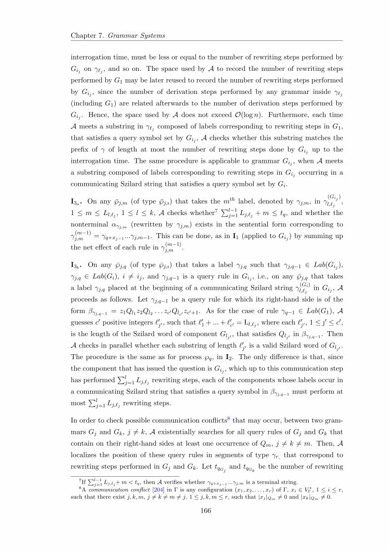
Chapter 7. Grammar Systems
interrogation time, must be less or equal to the number of rewriting steps performed by
Gij on γ`j , and so on. The space used by A to record the number of rewriting steps
performed by G1 may be later reused to record the number of rewriting steps performed
by Gij , since the number of derivation steps performed by any grammar inside γ`j
(including G1) are related afterwards to the number of derivation steps performed by
Gij . Hence, the space used by A does not exceed O(log n). Furthermore, each time
A meets a substring in γ`j composed of labels corresponding to rewriting steps in G1,
that satisfies a query symbol set by Gij , A checks whether this substring matches the
prefix of γ of length at most the number of rewriting steps done by Gij up to the
interrogation time. The same procedure is applicable to grammar Gij , when A meets
a substring composed of labels corresponding to rewriting steps in Gij occurring in a
communicating Szilard string that satisfies a query symbol set by Gi.
I3a. On any ℘j,m (of type ℘j,ı) that takes the mth label, denoted by γj,m, in γ(Gij )
l,`j,
1 ≤ m ≤ Ll,`j , 1 ≤ l ≤ k, A checks whether7∑l−1
j=1 Lj,`j + m ≤ tq, and whether the
nonterminal αγj,m (rewritten by γj,m) exists in the sentential form corresponding to
γ(m−1)j,m = γq+xj−1 ...γj,m−1. This can be done, as in I1 (applied to Gij ) by summing up
the net effect of each rule in γ(m−1)j,m .
I3b. On any ℘j,q (of type ℘j,ı) that takes a label γj,q such that γj,q−1 ∈ Lab(Gij ),
γj,q ∈ Lab(Gi), i 6= ij , and γj,q−1 is a query rule in Gij , i.e., on any ℘j,q that takes
a label γj,q placed at the beginning of a communicating Szilard string γ(Gi)l,`j
in Gij , Aproceeds as follows. Let γj,q−1 be a query rule for which its right-hand side is of the
form βγj,q−1 = z1Ql1z2Ql2 . . . zc′Qlc′zc′+1. As for the case of rule γq−1 ∈ Lab(G1), Aguesses c′ positive integers `′j′ , such that `′1 + ...+ `′c′ = Ll,`j , where each `′j′ , 1 ≤ ′ ≤ c′,is the length of the Szilard word of component Glj′ , that satisfies Qlj′ in βγj,q−1 . Then
A checks in parallel whether each substring of length `′j′ is a valid Szilard word of Glj′ .
The procedure is the same as for process ℘q, in I2. The only difference is that, since
the component that has issued the question is Gij , which up to this communication step
has performed∑l
j=1 Lj,`j rewriting steps, each of the components whose labels occur in
a communicating Szilard string that satisfies a query symbol in βγj,q−1 must perform at
most∑l
j=1 Lj,`j rewriting steps.
In order to check possible communication conflicts8 that may occur, between two gram-
mars Gj and Gk, j 6= k, A existentially searches for all query rules of Gj and Gk that
contain on their right-hand sides at least one occurrence of Qm, j 6= k 6= m. Then, Alocalizes the position of these query rules in segments of type γr that correspond to
rewriting steps performed in Gj and Gk. Let tqGj and tqGk be the number of rewriting
7If∑l−1j=1 Lj,`j+m < tq, then A verifies whether γq+xj−1 ...γj,m is a terminal string.
8A communication conflict [204] in Γ is any configuration (x1, x2, . . . , xr) of Γ, xi ∈ V ∗Γ , 1 ≤ i ≤ r,such that there exist j, k,m, j 6= k 6= m 6= j, 1 ≤ j, k,m ≤ r, such that |xj |Qm 6= 0 and |xk|Qm 6= 0.
166
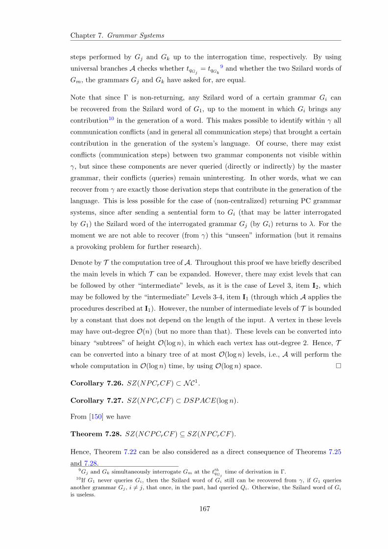
Chapter 7. Grammar Systems
steps performed by Gj and Gk up to the interrogation time, respectively. By using
universal branches A checks whether tqGj = tqGk9 and whether the two Szilard words of
Gm, the grammars Gj and Gk have asked for, are equal.
Note that since Γ is non-returning, any Szilard word of a certain grammar Gi can
be recovered from the Szilard word of G1, up to the moment in which Gi brings any
contribution10 in the generation of a word. This makes possible to identify within γ all
communication conflicts (and in general all communication steps) that brought a certain
contribution in the generation of the system’s language. Of course, there may exist
conflicts (communication steps) between two grammar components not visible within
γ, but since these components are never queried (directly or indirectly) by the master
grammar, their conflicts (queries) remain uninteresting. In other words, what we can
recover from γ are exactly those derivation steps that contribute in the generation of the
language. This is less possible for the case of (non-centralized) returning PC grammar
systems, since after sending a sentential form to Gi (that may be latter interrogated
by G1) the Szilard word of the interrogated grammar Gj (by Gi) returns to λ. For the
moment we are not able to recover (from γ) this “unseen” information (but it remains
a provoking problem for further research).
Denote by T the computation tree of A. Throughout this proof we have briefly described
the main levels in which T can be expanded. However, there may exist levels that can
be followed by other “intermediate” levels, as it is the case of Level 3, item I2, which
may be followed by the “intermediate” Levels 3-4, item I1 (through which A applies the
procedures described at I1). However, the number of intermediate levels of T is bounded
by a constant that does not depend on the length of the input. A vertex in these levels
may have out-degree O(n) (but no more than that). These levels can be converted into
binary “subtrees” of height O(log n), in which each vertex has out-degree 2. Hence, Tcan be converted into a binary tree of at most O(log n) levels, i.e., A will perform the
whole computation in O(log n) time, by using O(log n) space.
Corollary 7.26. SZ(NPCrCF ) ⊂ NC1.
Corollary 7.27. SZ(NPCrCF ) ⊂ DSPACE(log n).
From [150] we have
Theorem 7.28. SZ(NCPCrCF ) ⊆ SZ(NPCrCF ).
Hence, Theorem 7.22 can be also considered as a direct consequence of Theorems 7.25
and 7.28.9Gj and Gk simultaneously interrogate Gm at the tthqGj
time of derivation in Γ.10If G1 never queries Gi, then the Szilard word of Gi still can be recovered from γ, if G1 queries
another grammar Gj , i 6= j, that once, in the past, had queried Qi. Otherwise, the Szilard word of Giis useless.
167
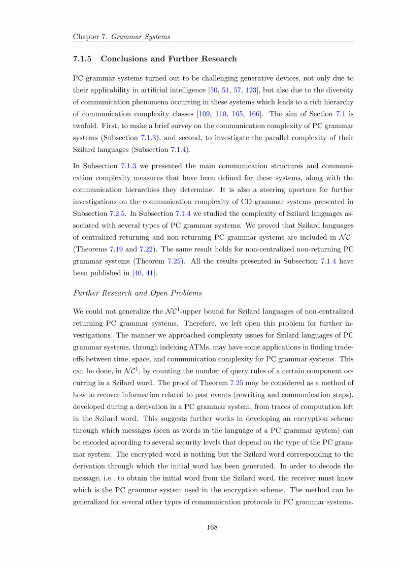
Chapter 7. Grammar Systems
7.1.5 Conclusions and Further Research
PC grammar systems turned out to be challenging generative devices, not only due to
their applicability in artificial intelligence [50, 51, 57, 123], but also due to the diversity
of communication phenomena occurring in these systems which leads to a rich hierarchy
of communication complexity classes [109, 110, 165, 166]. The aim of Section 7.1 is
twofold. First, to make a brief survey on the communication complexity of PC grammar
systems (Subsection 7.1.3), and second, to investigate the parallel complexity of their
Szilard languages (Subsection 7.1.4).
In Subsection 7.1.3 we presented the main communication structures and communi-
cation complexity measures that have been defined for these systems, along with the
communication hierarchies they determine. It is also a steering aperture for further
investigations on the communication complexity of CD grammar systems presented in
Subsection 7.2.5. In Subsection 7.1.4 we studied the complexity of Szilard languages as-
sociated with several types of PC grammar systems. We proved that Szilard languages
of centralized returning and non-returning PC grammar systems are included in NC1
(Theorems 7.19 and 7.22). The same result holds for non-centralized non-returning PC
grammar systems (Theorem 7.25). All the results presented in Subsection 7.1.4 have
been published in [40, 41].
Further Research and Open Problems
We could not generalize the NC1-upper bound for Szilard languages of non-centralized
returning PC grammar systems. Therefore, we left open this problem for further in-
vestigations. The manner we approached complexity issues for Szilard languages of PC
grammar systems, through indexing ATMs, may have some applications in finding trade-
offs between time, space, and communication complexity for PC grammar systems. This
can be done, in NC1, by counting the number of query rules of a certain component oc-
curring in a Szilard word. The proof of Theorem 7.25 may be considered as a method of
how to recover information related to past events (rewriting and communication steps),
developed during a derivation in a PC grammar system, from traces of computation left
in the Szilard word. This suggests further works in developing an encryption scheme
through which messages (seen as words in the language of a PC grammar system) can
be encoded according to several security levels that depend on the type of the PC gram-
mar system. The encrypted word is nothing but the Szilard word corresponding to the
derivation through which the initial word has been generated. In order to decode the
message, i.e., to obtain the initial word from the Szilard word, the receiver must know
which is the PC grammar system used in the encryption scheme. The method can be
generalized for several other types of communication protocols in PC grammar systems.
168

Chapter 7. Grammar Systems
7.2 Cooperating Distributed Grammar Systems
7.2.1 Prerequisites
Informally, a cooperating distributed grammar system (CD grammar system) consists
of several Chomsky grammars (called components) that work together according to a
specified protocol of cooperation. All the grammar components have a common axiom
and a common sentential form. The system works sequentially by generating a single
language. At each moment only one grammar is active. The time a component is active,
i.e., rewrites nonterminals on a common sentential form, is decided by the protocol of
cooperation. This protocol consists of start and stop conditions such as derivation modes
(how many times rewriting rules of the same component can be applied), weak fairness
conditions (each component has to be activated almost the same number of times) or
strong fairness conditions (each component has to be activated almost the same number
of times, by taking into account the number of internal productions that are applied for
each grammar). The model simulates the blackboard architecture in cooperative problem
solving considered at the level of symbol systems. In this model, the blackboard is the
common sentential form, and the system’s components are knowledge sources (agents,
processors, computer networks, etc.) [48, 50, 51].
The most important derivation modes defined in the literature are = k, ≤ k, ≥ k, t-
and ∗ - derivation modes, i.e., each component, when active, has to perform exactly k
steps, at most k steps, at least k steps, as many steps as possible, and arbitrarily many
steps, respectively [48, 50]. Several competence-based protocols have been defined in
[10, 49, 55]. A component is = k, ≤ k, and ≥ k-competent on a sentential form, if it
is able to rewrite exactly, at most, and at least k distinct nonterminals occurring in a
sentential form, respectively. Once a component starts to be f -competent on a sentential
form, it has to continue the derivation as long as it is f -competent, f ∈ ≤ k,= k,≥ k,k ≥ 1, on the newest sentential form. According to [55], in a CD grammar system
with competence start and stop conditions a component is able to start the derivation
if it satisfies a certain competence condition, settled as start condition. The component
works as long as it is competent on the current sentential form. It stops as soon as it
satisfies a certain competence-based stop condition. Formally we have [61]
Definition 7.29. A cooperating distributed grammar system of degree s, is an (s + 3)-
tuple Γ = (N,T, α, P1, . . . , Ps), where N and T are disjoint alphabets, the nonterminal
and terminal alphabet, respectively. P1, . . . , Ps are finite subsets of N × (N ∪T )∗ called
components, and α ∈ (N ∪ T )+ is the system axiom11.
11Note that, for the case when α ∈ N , we use for the system axiom, the S-notation (S ∈ N) insteadof the α-notation (see for instance Subsections 7.2.4 and 7.2.5).
169
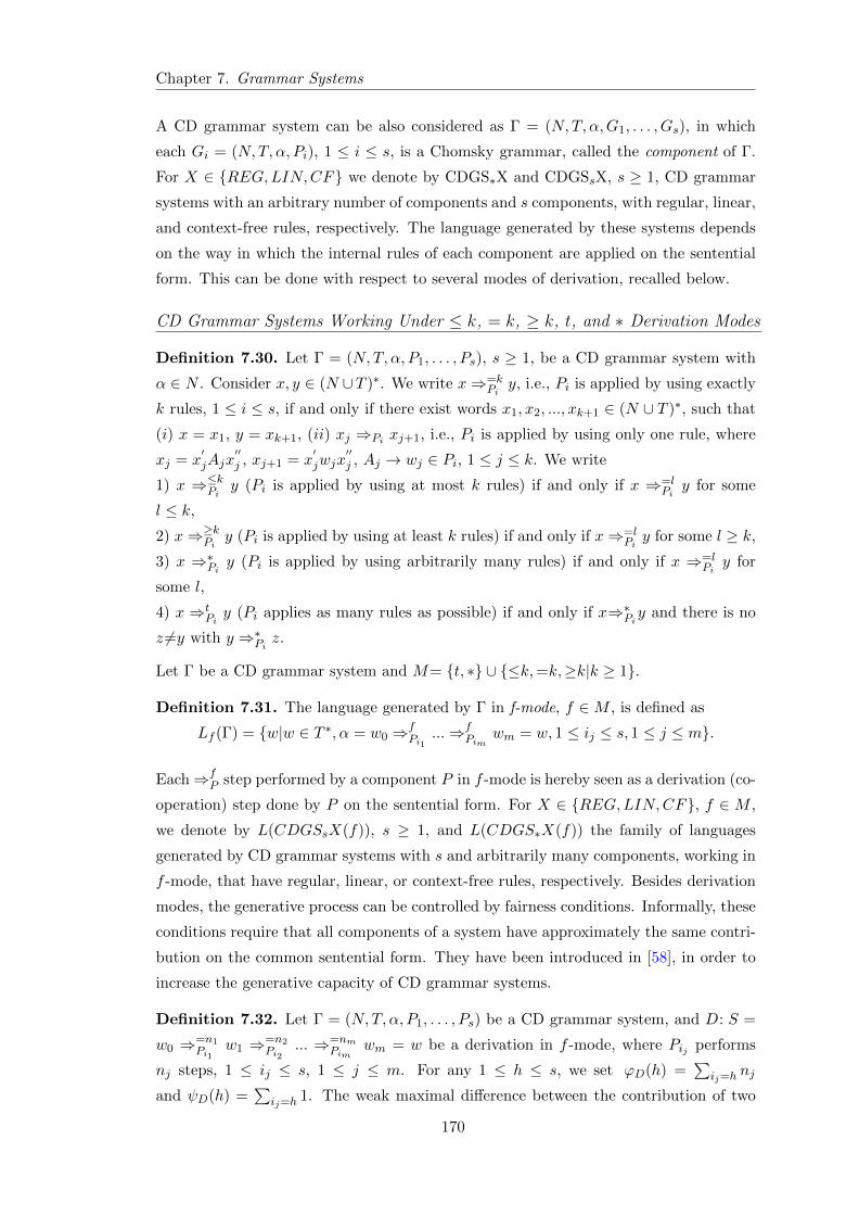
Chapter 7. Grammar Systems
A CD grammar system can be also considered as Γ = (N,T, α,G1, . . . , Gs), in which
each Gi = (N,T, α, Pi), 1 ≤ i ≤ s, is a Chomsky grammar, called the component of Γ.
For X ∈ REG,LIN,CF we denote by CDGS∗X and CDGSsX, s ≥ 1, CD grammar
systems with an arbitrary number of components and s components, with regular, linear,
and context-free rules, respectively. The language generated by these systems depends
on the way in which the internal rules of each component are applied on the sentential
form. This can be done with respect to several modes of derivation, recalled below.
CD Grammar Systems Working Under ≤ k, = k, ≥ k, t, and ∗ Derivation Modes
Definition 7.30. Let Γ = (N,T, α, P1, . . . , Ps), s ≥ 1, be a CD grammar system with
α ∈ N . Consider x, y ∈ (N ∪T )∗. We write x⇒=kPi
y, i.e., Pi is applied by using exactly
k rules, 1 ≤ i ≤ s, if and only if there exist words x1, x2, ..., xk+1 ∈ (N ∪ T )∗, such that
(i) x = x1, y = xk+1, (ii) xj ⇒Pi xj+1, i.e., Pi is applied by using only one rule, where
xj = x′jAjx
′′j , xj+1 = x
′jwjx
′′j , Aj → wj ∈ Pi, 1 ≤ j ≤ k. We write
1) x ⇒≤kPi y (Pi is applied by using at most k rules) if and only if x ⇒=lPiy for some
l ≤ k,
2) x⇒≥kPi y (Pi is applied by using at least k rules) if and only if x⇒=lPiy for some l ≥ k,
3) x ⇒∗Pi y (Pi is applied by using arbitrarily many rules) if and only if x ⇒=lPiy for
some l,
4) x ⇒tPiy (Pi applies as many rules as possible) if and only if x⇒∗Piy and there is no
z 6=y with y ⇒∗Pi z.
Let Γ be a CD grammar system and M= t, ∗ ∪ ≤k,=k,≥k|k ≥ 1.
Definition 7.31. The language generated by Γ in f-mode, f ∈M , is defined as
Lf (Γ) = w|w ∈ T ∗, α = w0 ⇒fPi1
...⇒fPim
wm = w, 1 ≤ ij ≤ s, 1 ≤ j ≤ m.
Each⇒fP step performed by a component P in f -mode is hereby seen as a derivation (co-
operation) step done by P on the sentential form. For X ∈ REG,LIN,CF, f ∈ M ,
we denote by L(CDGSsX(f)), s ≥ 1, and L(CDGS∗X(f)) the family of languages
generated by CD grammar systems with s and arbitrarily many components, working in
f -mode, that have regular, linear, or context-free rules, respectively. Besides derivation
modes, the generative process can be controlled by fairness conditions. Informally, these
conditions require that all components of a system have approximately the same contri-
bution on the common sentential form. They have been introduced in [58], in order to
increase the generative capacity of CD grammar systems.
Definition 7.32. Let Γ = (N,T, α, P1, . . . , Ps) be a CD grammar system, and D: S =
w0 ⇒=n1Pi1
w1 ⇒=n2Pi2
... ⇒=nmPim
wm = w be a derivation in f -mode, where Pij performs
nj steps, 1 ≤ ij ≤ s, 1 ≤ j ≤ m. For any 1 ≤ h ≤ s, we set ϕD(h) =∑
ij=hnj
and ψD(h) =∑
ij=h1. The weak maximal difference between the contribution of two
170
Chapter 7. Grammar Systems
components involved in the derivation D is defined as
dw(D) = max|ψD(i)− ψD(j)| |1 ≤ i, j ≤ s.The strong maximal difference between the contribution of two components is
ds(D) = max|ϕD(i)− ϕD(j)| |1 ≤ i, j ≤ s.Let u ∈ w, s, x ∈ (N ∪ T )∗, f ∈M and
du(x, f) = mindu(D)|D is a derivation of x in f− mode.For a fixed natural number q ≥ 0,
- the weakly q-fair language generated by Γ in the f -mode is defined as
Lf (Γ, wq) = x|x ∈ Lf (Γ) and dw(x, f) ≤ q,- the strongly q-fair language generated by Γ in the f -mode is
Lf (Γ, sq) = x|x ∈ Lf (Γ) and ds(x, f) ≤ q.
Denote by L(CDGSsX(f, wq)) and L(CDGSsX(f, sq)), s ≥ 1, X ∈ REG,LIN,CF,f ∈ M , the family of weakly and strongly q-fair languages generated by CD grammar
systems with s components, with respectively regular, linear, or context-free compo-
nents, working in f -mode of derivation.
CD Grammar Systems Working Under Competence Derivation Protocols
Informally, we say that a component Pi has the level of competence ≤ k, = k or ≥ k,
k ≥ 1, on a certain sentential form x, x ∈ (N∪T )∗, if the component Pi is ≤k-competent,
=k-competent, or ≥k-competent on x, i.e., it is able to rewrite at most, exactly, or at
least k distinct nonterminals occurring in the sentential form, respectively. Once a
component starts to be f -competent on a sentential form, f ∈ ≤ k,= k,≥ k, k ≥ 1, it
has to continue the derivation as long as it is f -competent on the newest sentential form.
Competence-based derivation modes have been defined only for CD grammar systems
with context-free components. Formally, we have [10]
Definition 7.33. Let Γ = (N,T, α, P1, . . . , Ps) be a CD grammar system with α ∈(N ∪ T )+. Denote by dom(Pi)=A ∈ N |A → z ∈ Pi the domain of the component
Pi, 1 ≤ i ≤ s, and by alphN (x)=A ∈ N ||x|A > 0. We say that Pi is ≤k-competent,
=k-competent or ≥k-competent on a sentential form x, x ∈ (N ∪ T )∗, if and only if
|alphN (x) ∩ dom(Pi)| is less than k, equal with k, or greater than k, respectively.
Denote by clevi(x) the level of competence of a component Pi on x. The cooperation
protocol, based on the capability of the component Pi to be≤k-competent, =k-competent,
or ≥k-competent on x ∈ (N ∪ T )∗, is defined as follows [10].
Definition 7.34. Let Γ = (N,T, α, P1, . . . , Ps) be a CD grammar system with α ∈(N ∪ T )+. Suppose x, y ∈ (N ∪ T )∗ and 1 ≤ i ≤ s.1. We say that y is derived from x in the ≤k-competence mode, denoted by x⇒≤k-comp.
i
y, if and only if there is a derivation x = x0 ⇒i x1...⇒i xm−1 ⇒i xm = y such that
171
Chapter 7. Grammar Systems
(a) clevi(xj) ≤ k for 0 ≤ j < m and (i) clevi(xm) = 0 or (ii) y ∈ T ∗,(b) clevi(xj) ≤ k for 0 ≤ j < m and clevi(xm) > k.
2. We say that y is derived from x in the =k-competence mode, denoted by x⇒=k-comp.i
y, if and only if there is a derivation x = x0 ⇒i x1...⇒i xm−1 ⇒i xm = y such that
(a) clevi(xj) = k for 0 ≤ j < m and clevi(xm) 6= k or
(b) clevi(x0) = k, clevi(xj) ≤ k for 1 ≤ j ≤ m, and y ∈ T ∗.3. We have x ⇒≥k-comp.
i y if and only if there is a derivation x = x0 ⇒i x1... ⇒i
xm−1 ⇒i xm = y such that (a) clevi(xj) ≥ k for 0 ≤ j < m and clevi(xm) < k or
(b) clevi(x0) ≥ k, and y ∈ T ∗.
Let C = ≤ k-comp.,= k-comp.,≥ k-comp.|k ≥ 1, and let ⇒f denote ⇒fi , for 1 ≤ i ≤
s, f ∈ C. We denote by ⇒∗f the reflexive and transitive closure of ⇒f .
Definition 7.35. The language generated by Γ in f -mode of derivation, f ∈ C, is
Lf (Γ) = w ∈ T ∗|α⇒∗f w.
The family of languages generated by CD grammar systems, with context-free rules, in
f -mode of derivation, f ∈ C, is denoted by L(CDGS(f)).
Szilard Languages
Due to the sequential character of CD grammar systems, for the case of Szilard language
associated with derivations in these systems, it is more appropriate to label the set of
productions instead of the productions (as for the case of PC grammar systems). Hence,
if Γ = (N,T, α, P1, . . . , Ps) is a CD grammar system, to each set Pi we associate a unique
label i, 1 ≤ i ≤ s. From [59] we have the following definition of a Szilard language
associated to derivations in a CD grammar system.
Definition 7.36. Let Γ = (N,T, α, P1, . . . , Ps) be a CD grammar system, and D a
derivation in f -mode, f ∈ M , of a word w ∈ Lf (Γ), of the form D : α = w0 ⇒fPi1
w1 ⇒ Pi2fw2 ⇒Pi3
... ⇒fPim
wm = w. The Szilard (control) word associated with
the derivation D of w, is defined as γw(D) = i1i2...im. The Szilard language associ-
ated with terminal derivations in Γ, in f -mode, is defined as Sz(Γ, f) = γw(D)|w ∈Lf (Γ) and D is a derivation in f -mode, of w, f ∈M.
Denote by SZ(CDGSsCF (f)) (SZ(CDGS∗CF (f))) the family of Szilard languages
associated with CD grammar systems of degree s (with arbitrary many components,
respectively) with context-free rules, working in f -mode, f∈ M = t, ∗ ∪ ≤ k,=k,≥k|k ≥1. From [59] we have
Theorem 7.37. 1. SZ(CF ) ⊂ SZ(CDGS∗CF (= k)), for all k ≥ 1, where SZ(CF ) is
the family of Szilard languages associated with context-free languages.
172
Chapter 7. Grammar Systems
2. SZ(CDGS∗CF (= k)) ⊆ L(M,CF ), SZ(CDGS∗CF (≥ k)) ⊆ L(M,CF ), k ≥ 1.
3. SZ(CDGS2CF (≤ k)) and SZ(CDGS3CF (∗)) contain non-regular languages, k ≥ 1.
4. SZ(CDGS3CF (≤ k)) and SZ(CDGS4CF (∗)) contain non-context-free languages.
5. SZ(CF ) is incomparable with SZ(CDGS∗CF (∗)) and SZ(CDGS∗CF (≤ k)), k ≥ 2.
6. SZ(CF ) and SZ(CDGS∗CF (≥ k)), k ≥ 1, are incomparable.
7. SZ(CF ) ⊂ SZ(CDGS∗CF (≤ 1)).
For CD grammar systems working under competence-based cooperation protocols it is
significant to know how long a certain component is active. Therefore for these CD
grammar systems we give the following definition of a Szilard language [31].
Definition 7.38. Let Γ = (N,T, α, P1, . . . , Ps) be a CD grammar system, and let D be a
terminal derivation in f -mode, f ∈ C, D: α = w0 ⇒=n1Pi1
w1 ⇒=n2Pi2
w2...⇒=nmPim
wm = w,
f ∈M , where Pij performs nj steps, 1 ≤ ij ≤ s, 1 ≤ j ≤ m. Let w be an arbitrary word
in Lf (Γ). The Szilard word of w associated with D is defined as γw(D)= in11 in2
2 ...inmm ,
where ij is the label of the component Pij and nj is the number of times the component
Pij contributes on the sentential form when it is activated in the f -mode. The Szilard
language associated with terminal derivations in Γ is defined as Sz(Γ, f) = γw(D)|w ∈Lf (Γ) and D a derivation in f -mode of w, f ∈ C.
Denote by SZ(CDGS(f)) the family of Szilard languages associated with CD grammar
systems with context-free components working in f -mode, f ∈ C = ≤ k-comp.,=
k-comp.,≥ k-comp.|k ≥ 1.
7.2.2 Computational Power and Computational Complexity
The class of languages generated by CD grammar systems with regular and linear com-
ponents, working in f -mode of derivation, f ∈ M = t, ∗ ∪ ≤ k,= k,≥ k|k ≥ 1,coincides with the class of regular and linear context-free languages, respectively [50].
The generative power of CD grammar systems with context-free components depends
on the derivation modes as follows [50, 61].
Theorem 7.39.
1. L(CDGS∗CF (f)) = CFL, f ∈ = 1,≥ 1, ∗ ∪ ≤ k|k ≥ 1.2. CFL = L(CDGSrCF (= 1)) = L(CDGSrCF (≤ k)) = L(CDGSrCF (∗)), r ≥ 1.
3. CFL = L(CDGS1CF (t)) = L(CDGS2CF (t)) ⊂ L(CDGSrCF (t)) = L(CDGS∗CF (t))
= ET0L, for r ≥ 3.
4. CFL = L(CDGS1CF (f))⊂ L(CDGS2CF (f))⊆ L(CDGSrCF (f))⊆ L(CDGS∗CF (f))
⊆ L(M,CF ), for r ≥ 3, f ∈ = k,≥ k|k ≥ 2.5. L(CDGSrCF (= k)) ⊆ L(CDGSrCF (= sk)), for all k, r, s ≥ 1.
6. L(CDGSrCF (≥ k)) ⊆ L(CDGSrCF (≥ k + 1)), for all k, r ≥ 1.
173

Chapter 7. Grammar Systems
For CD grammar systems working under competence-based protocols we have [10]
Theorem 7.40.
1. L(CDGS(f)) = L(RC,CF, ac) = REL, f ∈ ≤ k-comp.,= k-comp., k ≥ 2.
2. L(fRC,CF ) ⊆ L(CDGS(f), f ∈ ≤ 1-comp.,= 1-comp..3. L(CDGS(≥ 1-comp.)) = L(ETOL).
4. L(CDGS(≥ k-comp.)) = L(RC,ETOL, ac), k ≥ 2.
If instead of the t-mode of derivation the negated version is considered, i.e., the com-
ponents of the grammar system may stop rewriting only if they still have a production
applicable to the current sentential form, denoted by ¬t-mode, then L(CDGS(¬t))[16]⊂
L(RC,ETOL, ac). In [15, 16] several other relations between (random context) E(P)T0L
systems (see Section 6.4) and CD grammar systems that work in negated versions of the
classical derivation modes, defined in Definition 7.30, can be found.
7.2.3 A Simulation of CD Grammar Systems by Multicounter
Machines - Decidability Results
In this subsection we deal with CD grammar systems that use a special type of coop-
eration protocol based on the level of competence of a component to rewrite a certain
number of nonterminals occurring on the underlying sentential form. This competence-
based protocol has been introduced in [10]. Informally, a component is ≤ k-competent,
= k-competent or ≥ k-competent, k ≥ 1, on a certain sentential form if it is able to
rewrite at most, exactly, or at least k distinct nonterminals occurring in the sentential
form, respectively. Once a component starts to be f -competent on a sentential form,
f ∈ ≤ k,= k,≥ k, k ≥ 1, it has to continue the derivation as long as it is f -competent
on the newest sentential form. The formal definition of competence-based protocols
is provided in Subsection 7.2.1, Definition 7.34. In the sequel, we simulate CD gram-
mar systems working in f -competence mode, f ∈ ≤ k,= k,≥ k, k ≥ 1, by one-way
nondeterministic multicounter machines (Definition 4.11) performed in linear time and
space, with a linear-bounded number of reversals. For CD grammar systems working in
≤ 1,= 1-competence mode or in ≥ k-competence mode, k ≥ 1, the simulation is done
in quasirealtime by one-way partially blind multicounter machines (Definition 4.12).
Recall (see also Definition 4.11) that a multicounter machine, abbreviated MC, is an
accepting device composed of a finite state control, an input head, an input tape, and
a finite number of semi-infinite storage tapes that function as counters capable to store
any integer. For the case of a one-way multicounter, the input head is allowed to move
only to the right. If X is the input alphabet, then an input for a one-way MC is a string
of the form \w\, where \ is the input delimiter and w ∈ (X − \)∗. The machine starts
174
Chapter 7. Grammar Systems
in the initial state, with the input head placed on the left delimiter with all counters set
to zero. Each time the input head reads a symbol from the input tape, on a particular
state q, the machine checks the configuration of each counter, changes the value of each
counter by +1, -1, or 0, moves the head to the right and changes the state q into q′. The
input is accepted if the machine gets into a final state, with the input head placed on the
right delimiter, with empty counters. If the machine has at most one choice of action
on any configuration, then it is a deterministic MC. Otherwise, it is a nondeterministic
MC. Each choice of action is defined by a transition function δ. For the formal definition
of MC machines, complexity and hierarchy results on counter languages the reader is
referred to [24, 69, 81, 89, 90, 104, 106, 107, 111] (see also Subsection 4.2.3). From [31]
we have
Theorem 7.41. The Szilard language Sz(Γ, f) associated with a CD grammar system
Γ, working in f -mode, f ∈ C, can be recognized by an one-way nondeterministic m-
multicounter machine, in linear time and space, within linear bounded reversals and
linear 0-tests, where m is the number of the system nonterminals.
Proof. Let Γ = (N,T, α, P1, . . . , Ps) be a CD grammar system working in f -mode, f ∈ C,
where C = ≤ k-comp.,= k-comp.,≥ k-comp.|k ≥ 1. We provide a proof for = k-
comp.-mode, k ≥ 1. For the other f -modes the proof is similar. Let us consider the
ordered set of nonterminals N = A1, A2, ..., Am, m ≥ k, and let P = 1, 2, ..., s be
the set of labels attached to each component in the system. Let M be the one-way
nondeterministic m-multicounter machine, having as alphabet the set P and as input a
word γw(D) ∈ P ∗ of length n. Each counter corresponds to a nonterminal in N . For
each 1 ≤ i ≤ m, we denote by Ci the counter associated with Ai. In order to keep
control of the numbers of nonterminals occurring in the axiom α we will consider an
initial state of the form qα = q[x1]...[xm−1][xm], in which12 xi = |α|Ai , for 1 ≤ i ≤ m.
The machine starts in qα with all counters set to zero, having the input head placed on
the first delimiter \. From the state qα the machine gets into the state13 q[x1−1]...[xm],
by reading λ and increasing the content of counter C1 by +1. The operation continues
until the system reaches the state q[0][x2]...[xm], using x1 transitions through which the
content of the first counter is increased by x1 = |α|A1 . When the first cell of the state
q[x1]...[xm] had been “reduced” to 0 the same operation continues with the second cell
“storing” the value x2, by increasing the content of the second counter by x2 = |α|A2 ,
and so on. These operations end when all the m cells from the initial state had been re-
duced to 0 and each counter Ci had been increased by xi = |α|Ai , 1 ≤ i ≤ m. All the
transitions14 proceed by reading no symbol from the input tape. Denote as q0 the state
12Within a cell each xi, 1 ≤ i ≤ m, is a symbol, while ”outside” the cell xi is a number.13By [x1 − 1] we understand here a notation and not the subtraction operation.14These transitions cannot go below zero, and due to this for a cell marked by 0 there is no transition
that modifies this cell.
175
Chapter 7. Grammar Systems
q[0]...[0][0]. From now on the MC machine simulates the work of the CD grammar system
in = k-comp.-mode, as follows.
Step 1. Let us suppose that the first symbol from γw(D) is the label e corresponding
to the component Pe, such that |dom(Pe)| ≥ k. First M checks whether Pe is = k-
competent on α, i.e., |dom(Pe) ∩ alphN (α)| = k, where alphN (α) = A ∈ N ||α|A > 0.This is done by checking in the state q0, through the δ function that definesM, whether
reading e there are exactly k counters, that correspond to the k nonterminals from
dom(Pe) ∩ alphN (α), that have positive values. If this condition does not hold, γw(D)
is rejected. This can be done by not defining the δ function when reading e in other
configurations than those mentioned before. ♦
Step 2. Suppose that each nonterminal Al ∈ dom(Pe) ∩ alphN (α) is rewritten by a rule
of the form Al → rhs(Al). Then the content of Cl is decreased by 1, and the value of
each counter Ci corresponding to Ai occurring in rhs(Al) is increased by 1, as many
times as the letter Ai occurs in rhs(Al). ♦
When a component Pe is = k-competent on a sentential form x,M nondeterministically
chooses which nonterminal from x is rewritten by Pe and which rule that rewrites the
chosen nonterminal is applied. In order to emphasize that component Pe has been
activated15 we let the machine M ends the procedure from Step 2 in state qe.
For the next label in γw(D), denoted as e′, the machine checks, in state qe by reading λ,
whether the former component Pe, is still = k-competent on the newest sentential form.
This is done analogously as in Step 1, taking x instead of α. If Pe is = k-competent
on x and e = e′, then the computation continues as in Step 2. If Pe is = k-competent
on x, and e 6= e′, then γw(D) is rejected. If Pe′ is = k-competent and Pe is not, the
same operations on counters, described at Step 2, are nondeterministically performed
for the component Pe′ . The procedure ends in the state qe′ in order to mark that the
component Pe′ became active. If Pe′ is not = k-competent then γw(D) is rejected.
Finally, γw(D) is accepted if and only if the machine ends the computation with the
input head placed on the last delimiter \, with all counters set to zero.
Clearly, the number of 0-tests is linearly related to the length of the Szilard word γw(D).
Each time the input head reads a label from γw(D), the machine decreases the content of
one counter and increases the contents of a constant number of other counters. Therefore,
the number of reversals cannot be constant or more than linear.
Denote by max(Ci) the maximum absolute value stored in the counter Ci. Then
max(Ci) ≤ |α|Ai + li, where li is the number of times the content of counter Ci is
15Following the definition of the = k-comp.-mode this grammar should be active as long as it is= k-competent, even if several other components are = k-competent in the newest sentential form, too.
176
Chapter 7. Grammar Systems
increased by 1 during the computation. It is clear that each li is upper bounded by n/2.
Therefore,∑m
i=1max(Ci) ≤ |α| + mn/2. These remarks justify our assertion that the
simulation is done in linear time and space, within O(n) reversals and O(n) 0-tests, in
terms of the length of the Szilard word.
For the other cases the simulation works analogously. For the ≤ k-comp.-mode, for
instance, when checking the ≤ k-competence of the component Pe, we should allow to
M nondeterministically verify whether at most k counters corresponding to nonterminals
from dom(Pe) ∩ alphN (α), have positive values. For the next label e′ from γw(D), when
checking the ≤ k-competence of Pe′ and the non ≤ k-competence of Pe on the newest
sentential form x, where Pe has been previously applied, we check whether there are
at most k positive counters corresponding to at most k nonterminals from dom(Pe′) ∩alphN (x), and all counters corresponding to nonterminals from dom(Pe) ∩ alphN (x) are
zero, where alphN (x)=A ∈ N ||x|A > 0.
Our next approach is based on the notion of cycles introduced in [68, 106, 107] in
order to describe the structure of the words belonging to languages recognizable by MC
machines and used to prove closure properties for these languages. Each time a MC
machine reads a group of identical symbols whose number is greater than the number
of states, the device enters in a cycle, i.e., a part of the computation delimited by two
equal states q (the beginning and the end of the cycle) such that no further state q and
no two equal states, different from q, occur in the part of computation from q to q. We
say that this part of the computation is a cycle with state characteristic q, reading head
characteristic h, i.e., the symbol read by the reading head, and counter characteristic c,
for each counter, i.e., the difference between the counter contents at the beginning and
end of the cycle. For a MC machine with k counters and s states the number of cycles
with different characteristics is bounded by the constant s · s · (2s+ 1)k.
Using the above structural characterization of languages accepted by a MC machine,
Theorem 7.41 implies a kind of cyclicity phenomenon in the structure of the words
belonging to the Szilard language associated with a CD grammar system working in
competence mode in terms of state, head and counter characteristics. Based on this
remark we have
Lemma 7.42. Let Γ be a CD grammar system. The Szilard word γw(D) of a word
w ∈ Lf (Γ), f ∈ C, associated with a terminal derivation D performed in f -mode,
can be written in terms of a MC state, head and counter characteristics, of the form
γw(M) = z1on11 z2o
n22 ...zco
ncc zc+1, where zi, 1 ≤ i ≤ c+ 1, are finite subwords containing
no cycles, oj’s are finite cycles and nj, 1 ≤ j ≤ c, represents the number of times oj is
consecutively repeated.
177
Chapter 7. Grammar Systems
Note that in the Szilard word given by Lemma 7.42, each segment zi and oj is a sequence
of the form z1i ...z
pii and o1
j ...orjj , 1 ≤ i ≤ c+ 1 and 1 ≤ j ≤ c, respectively. Each zpi and
orj , where 1 ≤ p ≤ pi and 1 ≤ r ≤ rj , is a symbol that encodes three parameters, the
state characteristic q of M, the reading head characteristic h, i.e., the symbol read by
M in state q, and the counter characteristic c, i.e., the content of the counter in state
q. The length of γw(M) might be greater than the length of γw(D) due to the fact that
several zpi and orj symbols might have a head characteristic 0, i.e., the MC in the proof
of Theorem 7.41 reads λ. The relation between the length of γw(D) and the length of
γw(M) is |γw(M)| = d+ |γw(D)| where d ≤ q|γw(D)|, because the machineM works in
linear time of delay d and q is a constant. Next we denote by c, z, and o, the maximum
of c, the maximum of the length of zi, 1 ≤ i ≤ c+ 1, and the maximum of the length of
oj , 1 ≤ j ≤ c, taken over all groups of Szilard words with the same structure given by
Lemma 7.42, respectively. Our aim is to refine the class of multicounters that simulate
CD grammar systems, in order to find decidability results for them.
A blind multicounter (see Definition 4.12) is a particular MC that does not depend on the
counters’ configurations, but only on states and input. A blind multicounter is unable to
test the signs of its counters. The computation ends when the machine enters in a final
state with empty counters. A partially blind multicounter (pBMC) is a blind MC for
which its counters store only natural numbers, they cannot be checked for zero, and the
computation blocks whenever at least one of the counters becomes negative. A pBMC
machine works in quasirealtime if there exists a constant d such that the length of each
part of any computation in which the reading head is stationary is bounded by d. We
have [31]
Theorem 7.43. The Szilard language Sz(Γ, f) of a CD grammar system Γ, working
in f -comp.-mode, f ∈ ≤ 1,= 1, can be recognized by an one-way nondeterministic
pBMC in quasirealtime by using at most r = z(c+ 1) + oc counters.
Proof. Let Γ = (N,T, α, P1, . . . , Ps) be a CD grammar system working in ≤ 1,= 1-comp.-mode. Consider the ordered set of nonterminals N = A1, A2, ..., Am, and let
P = 1, 2, ..., s be the set of labels attached to each component in the system. Let B be
a one-way nondeterministic pBMC with at most r =z(c+ 1) + oc counters, that has as
alphabet the set P , and as input a Szilard word γw(D) ∈ P ∗ of length n. According to
Lemma 7.42, γw(D) can be also rewritten in the form γw(M) = z1on11 z2o
n22 ...zco
ncc zc+1
in which the segments zj , zc+1, and oj are of the form z1j ...z
pjj , z1
c+1...zpc+1
c+1 , and o1j ...o
rjj ,
1 ≤ j ≤ c, respectively. According to the computation performed by the machine M in
Theorem 7.41, each symbol zpi and orj , 1 ≤ p ≤ pi and 1 ≤ r ≤ rj , is characterized by
three parameters, the state characteristic q ofM, the reading head characteristic h, and
the counter characteristic c. Using the head characteristic we can make a direct relation
178
Chapter 7. Grammar Systems
between the Szilard word γw(D) written as a sequence of labels from P and the Szilard
word γw(M) of the machine M, written as a sequence of symbols characterized by the
above MC’s parameters.
The r counters are associated only with nonterminals Ai ∈ N . The first m counters are
associated with the nonterminals Ai, 1 ≤ i ≤ m, in N , in one-to-one correspondence.
The other counters are used accordingly with the length of the segments zj and oj from
the Szilard word. Furthermore, we consider each state of B being of the form q[]...[][], in
which the ith cell [] stands for the ith nonterminal Ai, 1 ≤ i ≤ m, and the last cell stands
for the label from P corresponding to the component that is currently simulated.
Next we give the simulation for = 1-comp.-mode. For ≤ 1-comp.-mode the simulation
works analogously. The machine starts with all counters set to zero, having the input
head placed on the first delimiter \, and the initial state qα = q[x1]...[xm−1][xm][0], in
which16 xi = |α|Ai , for 1 ≤ i ≤ m. The last zero-cell in qα is kept for the grammar
system component that is activated at each step of computation. As in the previous
theorem from the state qα the machine gets into the state q[x1−1]...[xm][0], by reading
λ and increasing the content of counter C1 by 1. The operation continues until the
system reaches the state q[0][x2]...[xm][0], using x1 states through which the content of
the first counter is increased by x1 = |α|A1 . Due to the fact that this time we work
with blind counters, we are not able to see the value stored on them17. In order to be
able to manipulate this lack each cell in the state that is reduced to 0 will be marked
by +. In this way we can memorize in states which counter may be non-empty (and
therefore, the corresponding nonterminal may exist in the sentential form). Thus the
state q[0][x2]...[xm][0] becomes q[+][x2]...[xm][0].
When the first cell of the state q[x1]...[xm][0] had been “reduced” to + the same operation
continues with the second cell “storing” the value x2, by increasing the content of the
second counter by x2 = |α|A2 , and so on. These operations end when all the m cells
storing a “non-zero value”, in the initial state had been reduced to + and the content
of each counter Ci had been increased by xi = |α|Ai , 1 ≤ i ≤ m. Denote as qc the
state reached at the end of this procedure. The state qc has all cells corresponding
to nonterminals occurring in α marked by +, all cells corresponding to nonterminals
not-occurring in α marked by 0, and the last cell still 0, because none of the system
components has been activated so far. As in the previous theorem, all these transitions
proceed by reading no symbol from the input type. From now on the simulation of the
CD grammar system in the = 1-comp.-mode is performed as follows.
16Here xi, 1 ≤ i ≤ m, have the same significance as in the previous theorem.17However, once the content of a counter is increased by at least 1 (i.e., the computation works on
that branch) the corresponding counter stores a positive integer. Each time the content of a counter isdecreased by at least 1, the machine must guess whether the corresponding counter becomes empty ornot, since it is not possible to know exactly which is the value stored on that counter.
179
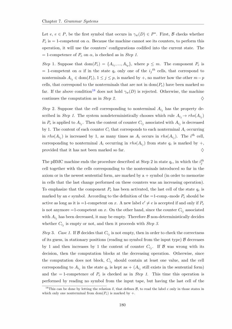
Chapter 7. Grammar Systems
Let e, e ∈ P , be the first symbol that occurs in γw(D) ∈ P ∗. First, B checks whether
Pe is = 1-competent on α. Because the machine cannot see its counters, to perform this
operation, it will use the counters’ configurations codified into the current state. The
= 1-competence of Pe on α, is checked as in Step 1.
Step 1. Suppose that dom(Pe) = Ai1 , ..., Aip, where p ≤ m. The component Pe is
= 1-competent on α if in the state qc only one of the ijth cells, that correspond to
nonterminals Aij ∈ dom(Pe), 1 ≤ j ≤ p, is marked by +, no matter how the other m−pcells, that correspond to the nonterminals that are not in dom(Pe) have been marked so
far. If the above condition18 does not hold γw(D) is rejected. Otherwise, the machine
continues the computation as in Step 2. ♦
Step 2. Suppose that the cell corresponding to nonterminal Aij has the property de-
scribed in Step 1. The system nondeterministically chooses which rule Aij→ rhs(Aij )
in Pe is applied to Aij . Then the content of counter Cij associated with Aij is decreased
by 1. The content of each counter Ci that corresponds to each nonterminal Ai occurring
in rhs(Aij ) is increased by 1, as many times as Ai occurs in rhs(Aij ). The ith cell,
corresponding to nonterminal Ai occurring in rhs(Aij ) from state qc is marked by +,
provided that it has not been marked so far. ♦
The pBMC machine ends the procedure described at Step 2 in state qe, in which the ithj
cell together with the cells corresponding to the nonterminals introduced so far in the
axiom or in the newest sentential form, are marked by a + symbol (in order to memorize
in cells that the last change performed on these counters was an increasing operation).
To emphasize that the component Pe has been activated, the last cell of the state qe is
marked by an e symbol. According to the definition of the =1-comp.-mode Pe should be
active as long as it is =1-competent on x. A new label e′ 6= e is accepted if and only if Pe
is not anymore =1-competent on x. On the other hand, since the counter Cij associated
with Aij has been decreased, it may be empty. Therefore B non-deterministically decides
whether Cij is empty or not, and then it proceeds with Step 3.
Step 3. Case 1. If B decides that Cij is not empty, then in order to check the correctness
of its guess, in stationary positions (reading no symbol from the input type) B decreases
by 1 and then increases by 1 the content of counter Cij . If B was wrong with its
decision, then the computation blocks at the decreasing operation. Otherwise, since
the computation does not block, Cij should contain at least one value, and the cell
corresponding to Aij in the state qe is kept as + (Aij still exists in the sentential form)
and the = 1-competence of Pe is checked as in Step 1. This time this operation is
performed by reading no symbol from the input tape, but having the last cell of the
18This can be done by letting the relation δ, that defines B, to read the label e only in those states inwhich only one nonterminal from dom(Pe) is marked by +.
180
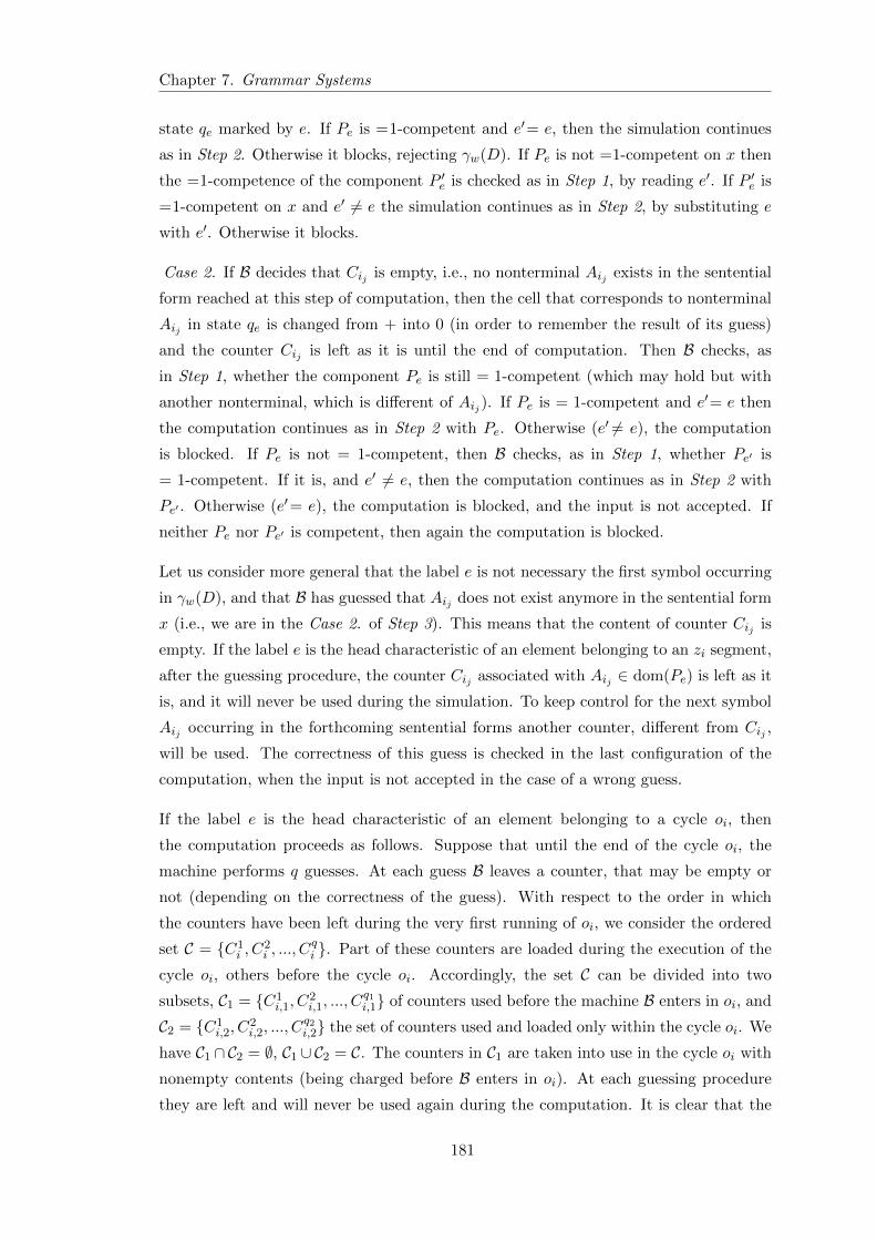
Chapter 7. Grammar Systems
state qe marked by e. If Pe is =1-competent and e′= e, then the simulation continues
as in Step 2. Otherwise it blocks, rejecting γw(D). If Pe is not =1-competent on x then
the =1-competence of the component P ′e is checked as in Step 1, by reading e′. If P ′e is
=1-competent on x and e′ 6= e the simulation continues as in Step 2, by substituting e
with e′. Otherwise it blocks.
Case 2. If B decides that Cij is empty, i.e., no nonterminal Aij exists in the sentential
form reached at this step of computation, then the cell that corresponds to nonterminal
Aij in state qe is changed from + into 0 (in order to remember the result of its guess)
and the counter Cij is left as it is until the end of computation. Then B checks, as
in Step 1, whether the component Pe is still = 1-competent (which may hold but with
another nonterminal, which is different of Aij ). If Pe is = 1-competent and e′= e then
the computation continues as in Step 2 with Pe. Otherwise (e′ 6= e), the computation
is blocked. If Pe is not = 1-competent, then B checks, as in Step 1, whether Pe′ is
= 1-competent. If it is, and e′ 6= e, then the computation continues as in Step 2 with
Pe′ . Otherwise (e′= e), the computation is blocked, and the input is not accepted. If
neither Pe nor Pe′ is competent, then again the computation is blocked.
Let us consider more general that the label e is not necessary the first symbol occurring
in γw(D), and that B has guessed that Aij does not exist anymore in the sentential form
x (i.e., we are in the Case 2. of Step 3). This means that the content of counter Cij is
empty. If the label e is the head characteristic of an element belonging to an zi segment,
after the guessing procedure, the counter Cij associated with Aij ∈ dom(Pe) is left as it
is, and it will never be used during the simulation. To keep control for the next symbol
Aij occurring in the forthcoming sentential forms another counter, different from Cij ,
will be used. The correctness of this guess is checked in the last configuration of the
computation, when the input is not accepted in the case of a wrong guess.
If the label e is the head characteristic of an element belonging to a cycle oi, then
the computation proceeds as follows. Suppose that until the end of the cycle oi, the
machine performs q guesses. At each guess B leaves a counter, that may be empty or
not (depending on the correctness of the guess). With respect to the order in which
the counters have been left during the very first running of oi, we consider the ordered
set C = C1i , C
2i , ..., C
qi . Part of these counters are loaded during the execution of the
cycle oi, others before the cycle oi. Accordingly, the set C can be divided into two
subsets, C1 = C1i,1, C
2i,1, ..., C
q1i,1 of counters used before the machine B enters in oi, and
C2 = C1i,2, C
2i,2, ..., C
q2i,2 the set of counters used and loaded only within the cycle oi. We
have C1 ∩ C2 = ∅, C1 ∪ C2 = C. The counters in C1 are taken into use in the cycle oi with
nonempty contents (being charged before B enters in oi). At each guessing procedure
they are left and will never be used again during the computation. It is clear that the
181
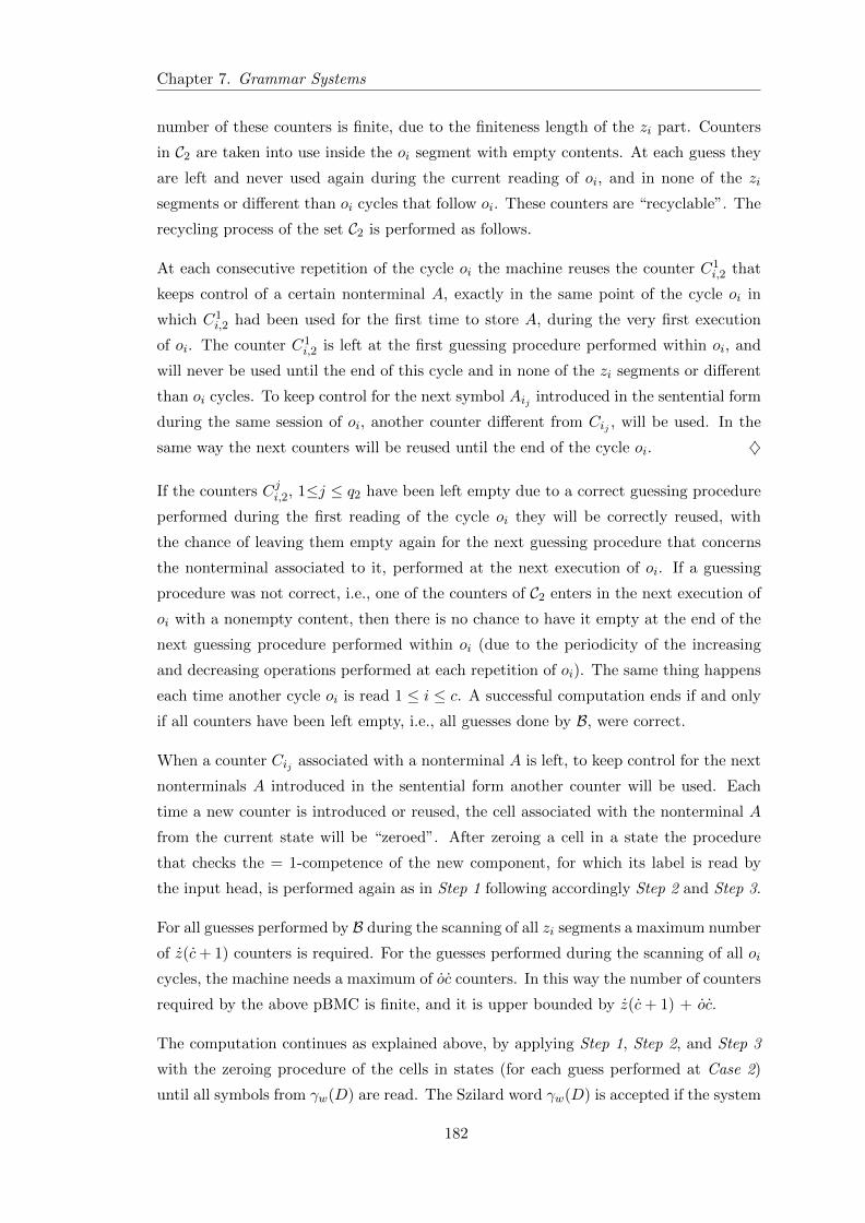
Chapter 7. Grammar Systems
number of these counters is finite, due to the finiteness length of the zi part. Counters
in C2 are taken into use inside the oi segment with empty contents. At each guess they
are left and never used again during the current reading of oi, and in none of the zi
segments or different than oi cycles that follow oi. These counters are “recyclable”. The
recycling process of the set C2 is performed as follows.
At each consecutive repetition of the cycle oi the machine reuses the counter C1i,2 that
keeps control of a certain nonterminal A, exactly in the same point of the cycle oi in
which C1i,2 had been used for the first time to store A, during the very first execution
of oi. The counter C1i,2 is left at the first guessing procedure performed within oi, and
will never be used until the end of this cycle and in none of the zi segments or different
than oi cycles. To keep control for the next symbol Aij introduced in the sentential form
during the same session of oi, another counter different from Cij , will be used. In the
same way the next counters will be reused until the end of the cycle oi. ♦
If the counters Cji,2, 1≤j ≤ q2 have been left empty due to a correct guessing procedure
performed during the first reading of the cycle oi they will be correctly reused, with
the chance of leaving them empty again for the next guessing procedure that concerns
the nonterminal associated to it, performed at the next execution of oi. If a guessing
procedure was not correct, i.e., one of the counters of C2 enters in the next execution of
oi with a nonempty content, then there is no chance to have it empty at the end of the
next guessing procedure performed within oi (due to the periodicity of the increasing
and decreasing operations performed at each repetition of oi). The same thing happens
each time another cycle oi is read 1 ≤ i ≤ c. A successful computation ends if and only
if all counters have been left empty, i.e., all guesses done by B, were correct.
When a counter Cij associated with a nonterminal A is left, to keep control for the next
nonterminals A introduced in the sentential form another counter will be used. Each
time a new counter is introduced or reused, the cell associated with the nonterminal A
from the current state will be “zeroed”. After zeroing a cell in a state the procedure
that checks the = 1-competence of the new component, for which its label is read by
the input head, is performed again as in Step 1 following accordingly Step 2 and Step 3.
For all guesses performed by B during the scanning of all zi segments a maximum number
of z(c+ 1) counters is required. For the guesses performed during the scanning of all oi
cycles, the machine needs a maximum of oc counters. In this way the number of counters
required by the above pBMC is finite, and it is upper bounded by z(c+ 1) + oc.
The computation continues as explained above, by applying Step 1, Step 2, and Step 3
with the zeroing procedure of the cells in states (for each guess performed at Case 2)
until all symbols from γw(D) are read. The Szilard word γw(D) is accepted if the system
182
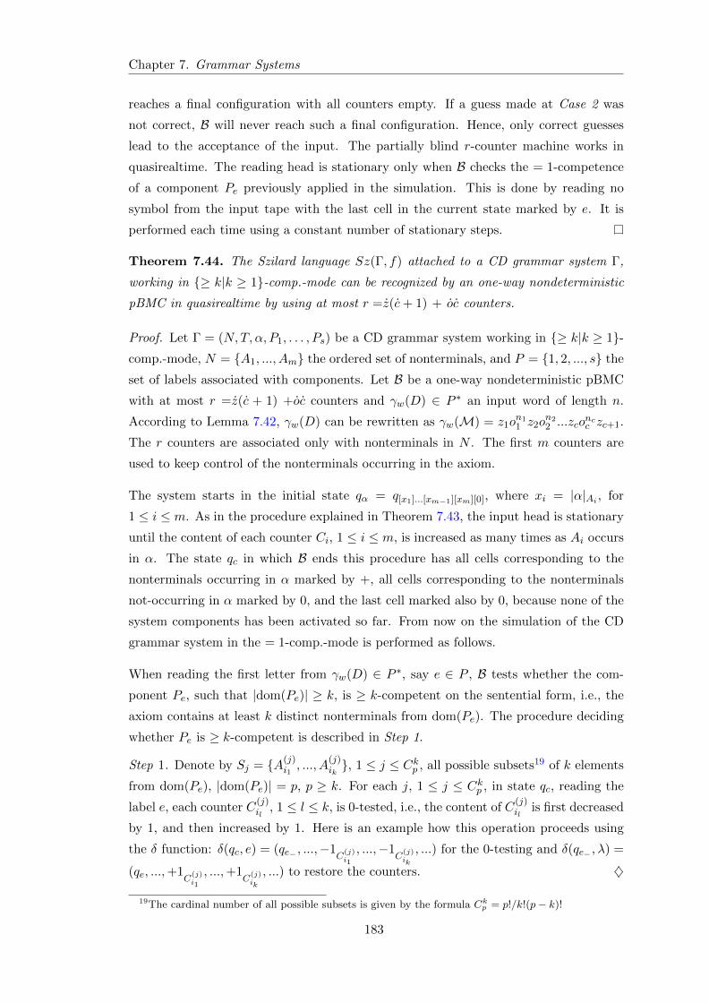
Chapter 7. Grammar Systems
reaches a final configuration with all counters empty. If a guess made at Case 2 was
not correct, B will never reach such a final configuration. Hence, only correct guesses
lead to the acceptance of the input. The partially blind r-counter machine works in
quasirealtime. The reading head is stationary only when B checks the = 1-competence
of a component Pe previously applied in the simulation. This is done by reading no
symbol from the input tape with the last cell in the current state marked by e. It is
performed each time using a constant number of stationary steps.
Theorem 7.44. The Szilard language Sz(Γ, f) attached to a CD grammar system Γ,
working in ≥ k|k ≥ 1-comp.-mode can be recognized by an one-way nondeterministic
pBMC in quasirealtime by using at most r =z(c+ 1) + oc counters.
Proof. Let Γ = (N,T, α, P1, . . . , Ps) be a CD grammar system working in ≥ k|k ≥ 1-comp.-mode, N = A1, ..., Am the ordered set of nonterminals, and P = 1, 2, ..., s the
set of labels associated with components. Let B be a one-way nondeterministic pBMC
with at most r =z(c + 1) +oc counters and γw(D) ∈ P ∗ an input word of length n.
According to Lemma 7.42, γw(D) can be rewritten as γw(M) = z1on11 z2o
n22 ...zco
ncc zc+1.
The r counters are associated only with nonterminals in N . The first m counters are
used to keep control of the nonterminals occurring in the axiom.
The system starts in the initial state qα = q[x1]...[xm−1][xm][0], where xi = |α|Ai , for
1 ≤ i ≤ m. As in the procedure explained in Theorem 7.43, the input head is stationary
until the content of each counter Ci, 1 ≤ i ≤ m, is increased as many times as Ai occurs
in α. The state qc in which B ends this procedure has all cells corresponding to the
nonterminals occurring in α marked by +, all cells corresponding to the nonterminals
not-occurring in α marked by 0, and the last cell marked also by 0, because none of the
system components has been activated so far. From now on the simulation of the CD
grammar system in the = 1-comp.-mode is performed as follows.
When reading the first letter from γw(D) ∈ P ∗, say e ∈ P , B tests whether the com-
ponent Pe, such that |dom(Pe)| ≥ k, is ≥ k-competent on the sentential form, i.e., the
axiom contains at least k distinct nonterminals from dom(Pe). The procedure deciding
whether Pe is ≥ k-competent is described in Step 1.
Step 1. Denote by Sj = A(j)i1, ..., A
(j)ik, 1 ≤ j ≤ Ckp , all possible subsets19 of k elements
from dom(Pe), |dom(Pe)| = p, p ≥ k. For each j, 1 ≤ j ≤ Ckp , in state qc, reading the
label e, each counter C(j)il
, 1 ≤ l ≤ k, is 0-tested, i.e., the content of C(j)il
is first decreased
by 1, and then increased by 1. Here is an example how this operation proceeds using
the δ function: δ(qc, e) = (qe− , ...,−1C
(j)i1
, ...,−1C
(j)ik
, ...) for the 0-testing and δ(qe− , λ) =
(qe, ...,+1C
(j)i1
, ...,+1C
(j)ik
, ...) to restore the counters. ♦
19The cardinal number of all possible subsets is given by the formula Ckp = p!/k!(p− k)!
183
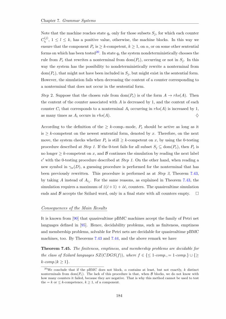
Chapter 7. Grammar Systems
Note that the machine reaches state qe only for those subsets Sj , for which each counter
C(j)il
, 1 ≤ l ≤ k, has a positive value, otherwise, the machine blocks. In this way we
ensure that the component Pe is ≥ k-competent, k ≥ 1, on α, or on some other sentential
forms on which has been tested20. In state qe the system nondeterministically chooses the
rule from Pe that rewrites a nonterminal from dom(Pe), occurring or not in Sj . In this
way the system has the possibility to nondeterministically rewrite a nonterminal from
dom(Pe), that might not have been included in Sj , but might exist in the sentential form.
However, the simulation fails when decreasing the content of a counter corresponding to
a nonterminal that does not occur in the sentential form.
Step 2. Suppose that the chosen rule from dom(Pe) is of the form A → rhs(A). Then
the content of the counter associated with A is decreased by 1, and the content of each
counter Ci that corresponds to a nonterminal Ai occurring in rhs(A) is increased by 1,
as many times as Ai occurs in rhs(A). ♦
According to the definition of the ≥ k-comp.-mode, Pe should be active as long as it
is ≥ k-competent on the newest sentential form, denoted by x. Therefore, on the next
move, the system checks whether Pe is still ≥ k-competent on x, by using the 0-testing
procedure described at Step 1. If the 0-test fails for all subset Sj ⊆ dom(Pe), then Pe is
no longer ≥ k-competent on x, and B continues the simulation by reading the next label
e′ with the 0-testing procedure described at Step 1. On the other hand, when reading a
new symbol in γw(D), a guessing procedure is performed for the nonterminal that has
been previously rewritten. This procedure is performed as at Step 3, Theorem 7.43,
by taking A instead of Aij . For the same reasons, as explained in Theorem 7.43, the
simulation requires a maximum of z(c+1) + oc, counters. The quasirealtime simulation
ends and B accepts the Szilard word, only in a final state with all counters empty.
Consequences of the Main Results
It is known from [90] that quasirealtime pBMC machines accept the family of Petri net
languages defined in [95]. Hence, decidability problems, such as finiteness, emptiness
and membership problems, solvable for Petri nets are decidable for quasirealtime pBMC
machines, too. By Theorems 7.43 and 7.44, and the above remark we have
Theorem 7.45. The finiteness, emptiness, and membership problems are decidable for
the class of Szilard languages SZ(CDGS(f)), where f ∈ ≤ 1-comp.,= 1-comp. ∪ ≥k-comp.|k ≥ 1.
20We conclude that if the pBMC does not block, α contains at least, but not exactly, k distinctnonterminals from dom(Pe). The lack of this procedure is that, when B blocks, we do not know withhow many counters it failed, because they are negative. That is why this method cannot be used to testthe = k or ≤ k-competence, k ≥ 1, of a component.
184
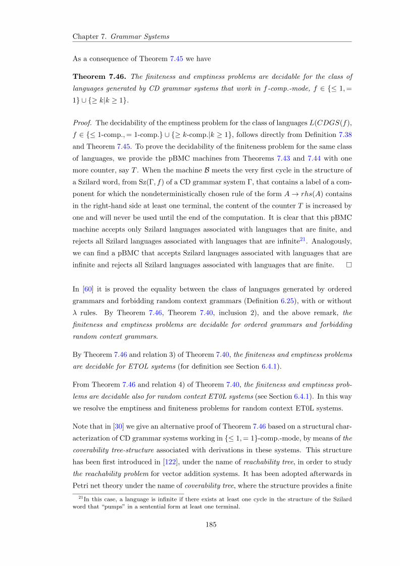
Chapter 7. Grammar Systems
As a consequence of Theorem 7.45 we have
Theorem 7.46. The finiteness and emptiness problems are decidable for the class of
languages generated by CD grammar systems that work in f -comp.-mode, f ∈ ≤ 1,=
1 ∪ ≥ k|k ≥ 1.
Proof. The decidability of the emptiness problem for the class of languages L(CDGS(f),
f ∈ ≤ 1-comp.,= 1-comp. ∪ ≥ k-comp.|k ≥ 1, follows directly from Definition 7.38
and Theorem 7.45. To prove the decidability of the finiteness problem for the same class
of languages, we provide the pBMC machines from Theorems 7.43 and 7.44 with one
more counter, say T . When the machine B meets the very first cycle in the structure of
a Szilard word, from Sz(Γ, f) of a CD grammar system Γ, that contains a label of a com-
ponent for which the nondeterministically chosen rule of the form A→ rhs(A) contains
in the right-hand side at least one terminal, the content of the counter T is increased by
one and will never be used until the end of the computation. It is clear that this pBMC
machine accepts only Szilard languages associated with languages that are finite, and
rejects all Szilard languages associated with languages that are infinite21. Analogously,
we can find a pBMC that accepts Szilard languages associated with languages that are
infinite and rejects all Szilard languages associated with languages that are finite.
In [60] it is proved the equality between the class of languages generated by ordered
grammars and forbidding random context grammars (Definition 6.25), with or without
λ rules. By Theorem 7.46, Theorem 7.40, inclusion 2), and the above remark, the
finiteness and emptiness problems are decidable for ordered grammars and forbidding
random context grammars.
By Theorem 7.46 and relation 3) of Theorem 7.40, the finiteness and emptiness problems
are decidable for ETOL systems (for definition see Section 6.4.1).
From Theorem 7.46 and relation 4) of Theorem 7.40, the finiteness and emptiness prob-
lems are decidable also for random context ET0L systems (see Section 6.4.1). In this way
we resolve the emptiness and finiteness problems for random context ET0L systems.
Note that in [30] we give an alternative proof of Theorem 7.46 based on a structural char-
acterization of CD grammar systems working in ≤ 1,= 1-comp.-mode, by means of the
coverability tree-structure associated with derivations in these systems. This structure
has been first introduced in [122], under the name of reachability tree, in order to study
the reachability problem for vector addition systems. It has been adopted afterwards in
Petri net theory under the name of coverability tree, where the structure provides a finite
21In this case, a language is infinite if there exists at least one cycle in the structure of the Szilardword that “pumps” in a sentential form at least one terminal.
185
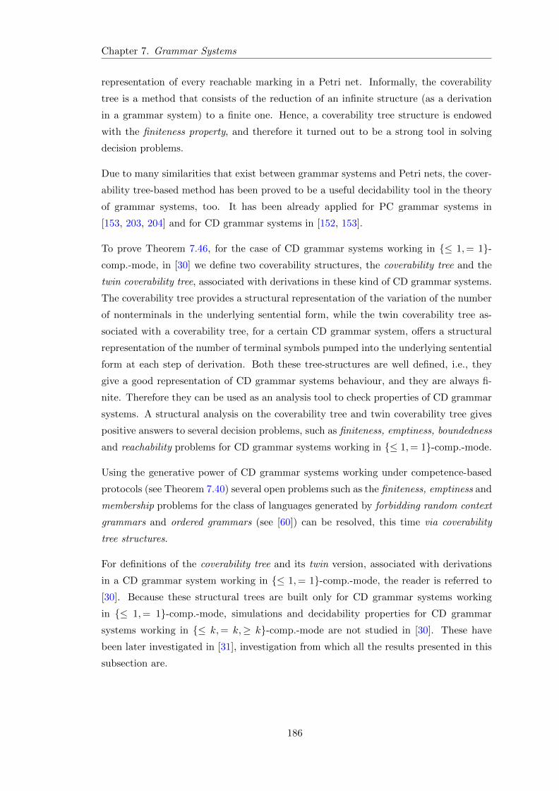
Chapter 7. Grammar Systems
representation of every reachable marking in a Petri net. Informally, the coverability
tree is a method that consists of the reduction of an infinite structure (as a derivation
in a grammar system) to a finite one. Hence, a coverability tree structure is endowed
with the finiteness property, and therefore it turned out to be a strong tool in solving
decision problems.
Due to many similarities that exist between grammar systems and Petri nets, the cover-
ability tree-based method has been proved to be a useful decidability tool in the theory
of grammar systems, too. It has been already applied for PC grammar systems in
[153, 203, 204] and for CD grammar systems in [152, 153].
To prove Theorem 7.46, for the case of CD grammar systems working in ≤ 1,= 1-comp.-mode, in [30] we define two coverability structures, the coverability tree and the
twin coverability tree, associated with derivations in these kind of CD grammar systems.
The coverability tree provides a structural representation of the variation of the number
of nonterminals in the underlying sentential form, while the twin coverability tree as-
sociated with a coverability tree, for a certain CD grammar system, offers a structural
representation of the number of terminal symbols pumped into the underlying sentential
form at each step of derivation. Both these tree-structures are well defined, i.e., they
give a good representation of CD grammar systems behaviour, and they are always fi-
nite. Therefore they can be used as an analysis tool to check properties of CD grammar
systems. A structural analysis on the coverability tree and twin coverability tree gives
positive answers to several decision problems, such as finiteness, emptiness, boundedness
and reachability problems for CD grammar systems working in ≤ 1,= 1-comp.-mode.
Using the generative power of CD grammar systems working under competence-based
protocols (see Theorem 7.40) several open problems such as the finiteness, emptiness and
membership problems for the class of languages generated by forbidding random context
grammars and ordered grammars (see [60]) can be resolved, this time via coverability
tree structures.
For definitions of the coverability tree and its twin version, associated with derivations
in a CD grammar system working in ≤ 1,= 1-comp.-mode, the reader is referred to
[30]. Because these structural trees are built only for CD grammar systems working
in ≤ 1,= 1-comp.-mode, simulations and decidability properties for CD grammar
systems working in ≤ k,= k,≥ k-comp.-mode are not studied in [30]. These have
been later investigated in [31], investigation from which all the results presented in this
subsection are.
186
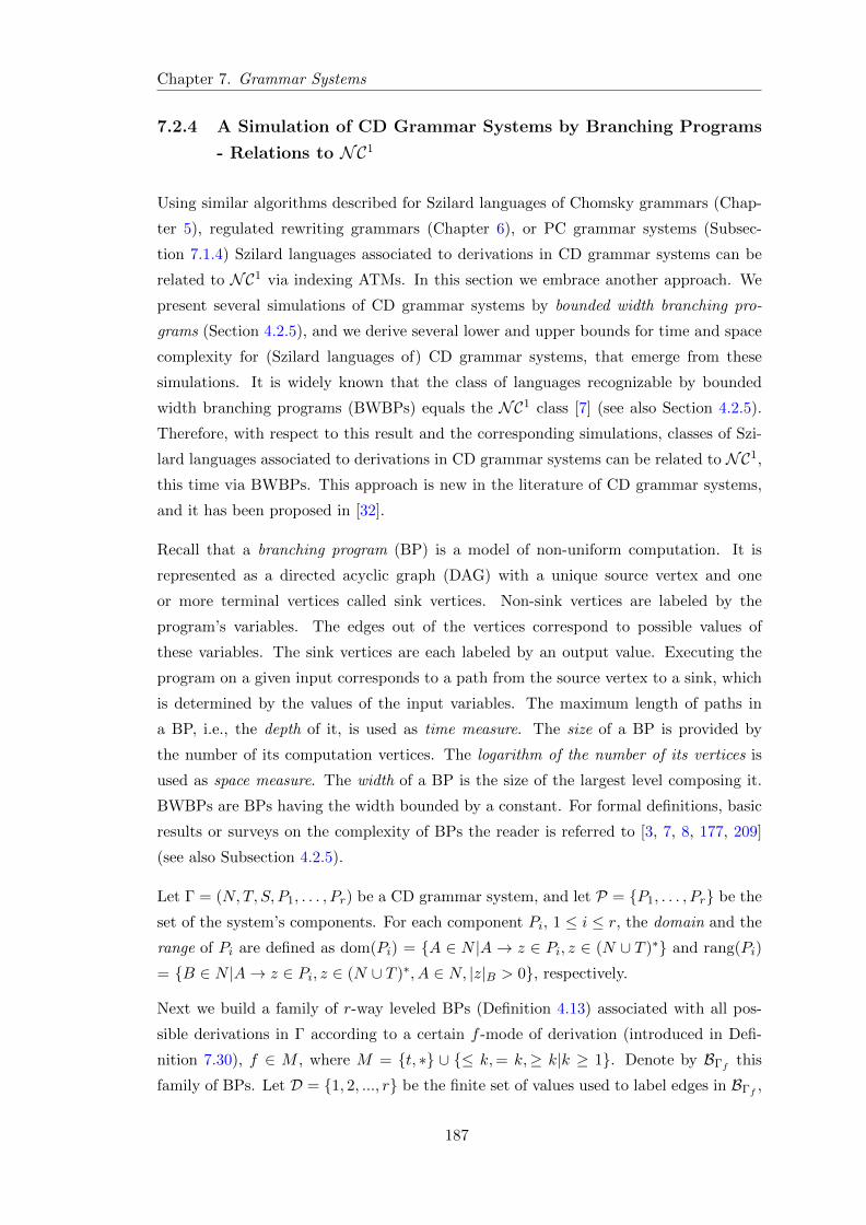
Chapter 7. Grammar Systems
7.2.4 A Simulation of CD Grammar Systems by Branching Programs
- Relations to NC1
Using similar algorithms described for Szilard languages of Chomsky grammars (Chap-
ter 5), regulated rewriting grammars (Chapter 6), or PC grammar systems (Subsec-
tion 7.1.4) Szilard languages associated to derivations in CD grammar systems can be
related to NC1 via indexing ATMs. In this section we embrace another approach. We
present several simulations of CD grammar systems by bounded width branching pro-
grams (Section 4.2.5), and we derive several lower and upper bounds for time and space
complexity for (Szilard languages of) CD grammar systems, that emerge from these
simulations. It is widely known that the class of languages recognizable by bounded
width branching programs (BWBPs) equals the NC1 class [7] (see also Section 4.2.5).
Therefore, with respect to this result and the corresponding simulations, classes of Szi-
lard languages associated to derivations in CD grammar systems can be related to NC1,
this time via BWBPs. This approach is new in the literature of CD grammar systems,
and it has been proposed in [32].
Recall that a branching program (BP) is a model of non-uniform computation. It is
represented as a directed acyclic graph (DAG) with a unique source vertex and one
or more terminal vertices called sink vertices. Non-sink vertices are labeled by the
program’s variables. The edges out of the vertices correspond to possible values of
these variables. The sink vertices are each labeled by an output value. Executing the
program on a given input corresponds to a path from the source vertex to a sink, which
is determined by the values of the input variables. The maximum length of paths in
a BP, i.e., the depth of it, is used as time measure. The size of a BP is provided by
the number of its computation vertices. The logarithm of the number of its vertices is
used as space measure. The width of a BP is the size of the largest level composing it.
BWBPs are BPs having the width bounded by a constant. For formal definitions, basic
results or surveys on the complexity of BPs the reader is referred to [3, 7, 8, 177, 209]
(see also Subsection 4.2.5).
Let Γ = (N,T, S, P1, . . . , Pr) be a CD grammar system, and let P = P1, . . . , Pr be the
set of the system’s components. For each component Pi, 1 ≤ i ≤ r, the domain and the
range of Pi are defined as dom(Pi) = A ∈ N |A → z ∈ Pi, z ∈ (N ∪ T )∗ and rang(Pi)
= B ∈ N |A→ z ∈ Pi, z ∈ (N ∪ T )∗, A ∈ N, |z|B > 0, respectively.
Next we build a family of r-way leveled BPs (Definition 4.13) associated with all pos-
sible derivations in Γ according to a certain f -mode of derivation (introduced in Defi-
nition 7.30), f ∈ M , where M = t, ∗ ∪ ≤ k,= k,≥ k|k ≥ 1. Denote by BΓf this
family of BPs. Let D = 1, 2, ..., r be the finite set of values used to label edges in BΓf ,
187
Chapter 7. Grammar Systems
and X = x0, x1, ..., xr be the set of variables over D. One of the sink vertex of BΓf is
labeled by 0, and it corresponds to an unaccepted word. The other sink vertex is labeled
by 1, and it corresponds to an accepted word. Only words corresponding to terminal
derivations in Γf are accepted. Let x0 be the variable set in the source vertex of BΓf , and
D0⊆ D, D0 = i10, i20, ..., ip00 , 1≤ p0≤ r, such that S∈ dom(P
ij10
), 1≤ j1≤ p0. According
to the manner in which Γf works, x0 may take one of the values in D0. Thus, edges
outgoing from x0 are labeled by distinct elements in D0. Accordingly, the computation
of BΓf proceeds, for each element ij10 ∈ D0, as follows.
To each edge labeled by ij10 we assign the sentential form wj10 , obtained when Pij10
stops to
be active, 1 ≤ j1 ≤ p0. In this moment either the derivation stops, because X||wj10 |X >
0, X ∈ N = ∅, i.e., wj10 ∈ Lf (Γ), and the edge labeled by ij10 and assigned with wj10 goes
into the sink vertex labeled by 1, or X||wj10 |X > 0, X ∈ N 6= ∅ and a new grammar
with P 6= Pij10
may become active. For the latter case consider the condition
(|wj10 |B > 0) ∧ (B ∈ rang(Pij10
) ∩ dom(P )). (7.1)
If there is no B ∈ N and P ∈ P satisfying (7.1), then the edge labeled by ij10 and assig-
ned with wj10 goes into the sink vertex labeled by 0. If there exist at least one non-
terminal B ∈ N and at least one grammar P ∈ P that satisfy (7.1), then due to the
nondeterministic character of CD grammar systems, each component P satisfying (7.1),
able to work in f -mode on wj10 , can continue the derivation. In this case, the edge
labeled by ij10 , 1≤ j1≤ p0, and assigned with wj10 , goes into a vertex labeled by xij10
.
Denote by D1j1
= i11j1 , i21j1, ..., i
p1j1
1j1, 1≤ p1
j1≤ r, the subset of D such that P
ij21j1
, Pij21j1
6=
Pij10
, satisfies (7.1) and Pij21j1
, 1 ≤ j2 ≤ p1j1
, is able to work in f -mode on wj10 . For each
i ∈ D − D1j1
, the computation of BΓf proceeds with a new edge labeled by i, outgoing
from xij10
and entering into the sink vertex labeled by 0.
For each ij21j1 ∈ D1j1
, 1≤ j2≤ p1j1
, the computation of BΓf proceeds with a new edge
outgoing from xij10
and labeled by ij21j1 . To this edge we assign the sentential form
obtained when grammar Pij21j1
stops to be active. Let wj21j1be this sentential form. In
this moment either the derivation stops on the branch j2, because X||wj21j1|X> 0, X∈
N = ∅, i.e., wj21j1∈ Lf (Γ), or X||wj21j1
|X> 0, X∈ N 6= ∅, and a new grammar P 6= Pij21j1
becomes active. In the first case an outgoing edge from xij10
, labeled by ij21j1 and assigned
with wj21j1, goes into the sink vertex labeled by 1, while in the second case the condition
(|wj21j1|B > 0) ∧ (B ∈ rang(P
ij21j1
) ∩ dom(P )) (7.2)
is tested for each j2, 1≤ j2≤ p1j1
, and each subset D1j1
, 1≤ j1≤ p0.
188
Chapter 7. Grammar Systems
If there is no B∈ N and P ∈ P satisfying (7.2), then BΓf proceeds on the j2 branch
corresponding to the subset D1j1
, with an edge labeled by ij21j1 and assigned with wj21j1
outgoing from xij10
and entering into the sink vertex labeled by 0. Otherwise, let D2j2
=
i12j2 , i22j2, ..., i
p2j2
2j2, 1≤ p2
j2≤ r, be the subset of D such that P
ij32j2
, 1≤ j3≤ p2j2
, satisfies
(7.2) and it is able to work in f -mode on wj21j1.
Suppose that we built all the vertices placed at the first level of BΓf , labeled by xij10
,
ij10 ∈D0, and we found all components that are able to continue the derivation on each
of the j1, 1≤ j1≤ p0, branches according to each subset D1j1
of D. We impose to all
edges labeled by the same value i ∈ D, to go into the same vertex labeled22 by the
variable xi, placed on the second level of BΓf . Therefore, at the second level of BΓf
there will be at most r vertices. Let us continue to build BΓf on branch j2, according
to D1j1
. The computation of BΓf is performed analogously on the other branches. For
each i ∈ D −D2j2
, the computation of BΓf proceeds with an edge labeled by i, outgoing
from the vertex labeled by xij21j1
, and going into the sink vertex labeled by 0.
For each ij32j2 ∈ D2j2
, the computation of BΓf proceeds with a new edge going from xij21j1
and labeled by ij32j2 , 1 ≤ j3 ≤ p2j2
. To this edge we assign a sentential form wj32j2obtained
when grammar Pij32j2
stops to be active. From now on, the computation of the third level
of BΓf is performed using the same procedure as for the second level. We sort out all
edges that go into sink vertices 0 and 1, and fix all vertices labeled by elements in D,
corresponding to components of Γ able to continue the derivation in f -mode.
Suppose that we built BΓf up to level k − 1, and we want to build the kth level. Con-
sider the variable xijk−1k−2jk−2
that labels a certain vertex placed at level k − 1, such that
the edge coming into this vertex, via the branch jk−1, is labeled by ijk−1
k−2jk−2and it is
assigned with the sentential form wjk−1
k−2jk−2. All these edges correspond to a subset of the
form Dk−2jk−2
= i1k−2jk−2, i2k−2jk−2
, ..., ipk−2jk−2
k−2jk−2, 1≤ pk−2
jk−2≤ r, such that each component
Pijk−1k−2jk−2
, 1≤ jk−1 ≤ pk−2jk−2
, is able to continue the derivation on the sentential form
wjk−1
k−2jk−2. Furthermore, as mentioned, edges labeled by the same value i ∈ D go into
the same vertex, labeled by xi placed at level k − 1. So that at this level there will
be at most r vertices. Now, we may have either X||wjk−1
k−2jk−2|X> 0, X∈ N = ∅, i.e.,
wjk−1
k−2jk−2∈ Lf (Γ), or X||wjk−1
k−2jk−2|X> 0, X∈ N 6= ∅, i.e., a new grammar P 6= P
ijk−1k−2jk−2
may become active. In the former case an outgoing edge from xijk−2k−3jk−3
, labeled by
ijk−1
k−2jk−2and assigned with w
jk−1
k−2jk−2goes into the sink vertex labeled by 1, while in the
latter case the condition
22Thus, all the vertices labeled by variables xij21j1
, for which all indexes ij21j1 , 1 ≤ j1 ≤ p0, 1 ≤ j2 ≤ p1j1 ,
take the same value i ∈ D, are gathered into a single vertex labeled by xi.
189
Chapter 7. Grammar Systems
(|wjk−1
k−2jk−2|B > 0) ∧ (B ∈ rang(P
ijk−1k−2jk−2
) ∩ dom(P )) (7.3)
is tested for each 1≤ jk−1≤ pk−2jk−2
.
If there is no B ∈ N and P ∈ P satisfying (7.3), then BΓf proceeds on branch jk−1
with an edge, labeled by ijk−1
k−2jk−2and assigned with w
jk−1
k−2jk−2, outgoing from the vertex
labeled by xijk−2k−3jk−3
and entering into the sink labeled by 0. Otherwise, consider Dk−1jk−1
=
i1k−1jk−1, i2k−1jk−1
, ..., ipk−1jk−1
k−1jk−1, 1≤ pk−1
jk−1≤ r, the subset ofD such that P
ijkk−1jk−1
, 1≤ jk≤
pk−1jk−1
, satisfies (7.3) and it is able to work in f -mode on wjk−1
k−2jk−2. For each i ∈ D−Dk−1
jk−1,
the computation of BΓf proceeds with a new edge, labeled by i, outgoing from xijk−1k−2jk−2
,
and entering into the sink vertex labeled by 0.
For each ijkk−1jk−1∈ Dk−1
jk−1, 1 ≤ jk ≤ pk−1
jk−1, the computation of BΓf proceeds with a
new edge outgoing from xijk−1k−2jk−2
, labeled by ijkk−1jk−1, and assigned with the sentential
form obtained when grammar Pijkk−1jk−1
stops to be active. Let wjkk−1jk−1be this sentential
form. In this moment either the derivation stops on branch jk, because X||wjkk−1jk−1|X>
0, X ∈ N =∅, i.e., wjkk−1jk−1∈ Lf (Γ), or X||wjkk−1jk−1
|X > 0, X ∈ N 6= ∅, and a new
grammar P 6= Pijkk−1jk−1
becomes active. In the former case an outgoing edge from
xijkk−1jk−1
labeled by ijkk−1jk−1and assigned with wjkk−1jk−1
goes into the sink labeled by 1,
while in the latter case the condition
(|wjkk−1jk−1|B > 0) ∧ (B ∈ rang(P
ijkk−1jk−1
) ∩ dom(P )) (7.4)
is tested for each 1≤ jk≤ pk−1jk−1
.
The computation of BΓf proceeds in the same way as before by sorting out all edges
going into 0 and 1 sink vertices, or those labeled by elements in D, corresponding to
components of Γ able to continue the derivation in f -mode. The procedure ends when
no level is possible to be built anymore, i.e., edges from vertices placed at the last level
go solely into sink vertices. Analyzing BΓf to be observed that each path from the source
vertex to a sink labeled by 1 represents the control Szilard word of the word generated
by Γf on that path. Hence BΓf accepts the Szilard language Sz(Γ, f) associated to Γf
and in the same time yields the language Lf (Γ) generated by Γf . Each BP belonging
to BΓf has the width r ≥ 2, so that BΓf is an r-way BWBP. According to the above
construction, we have [32]
Theorem 7.47. For each grammar system Γ, Γ ∈ CDGSrX, working in f -mode,
f ∈ M , X ∈ REG,LIN,CF, there exists a family of deterministic r-way BWBPs,
r ≥ 2, that accepts Sz(Γ, f) and generates Lf (Γ).
190
Chapter 7. Grammar Systems
Note that the deterministic r-way BWBP BΓf can be converted into a nondeterministic
Boolean BWBP. This can be achieved by taking as variables the grammar components
and labeling by 1 each edge that goes out from a vertex labeled by a component able to
continue the derivation in f -mode, and labeling by 0 each edge that goes out from ver-
tices labeled by idle components. Both families of BPs have the same time complexity.
The size of the Boolean BPs differs from the r-way BPs’ size by an log r factor. Consid-
ering a binary code for D = 1, 2, ..., r we can think to the Szilard language associated
with derivations in a CD grammar system as a language in 0, 1∗. In the sequel, for
a grammar system Γf , f ∈ M , we will denote by Sz0,1(Γ, f) a binary representation
of the Szilard language associated with derivations in Γf . The family of Sz0,1(Γ, f)
languages is denoted as ZSr0,1(f). By Theorem 7.47 and the above remark we have
Theorem 7.48. For each Γ, Γ ∈ CDGSrX, X ∈ REG,LIN,CF, working in f -
mode, f ∈ M , there exists a family of nondeterministic Boolean BWBPs, that accepts
Sz0,1(Γ, f) and generates Lf (Γ).
Depending on the mode of derivation in which a CD grammar system works we have
Theorem 7.49. For each grammar system Γ working in f -mode, f ∈ = 1,≥ 1, ∗∪≤k|k ≥ 1, Γ ∈ CDGSrX, r ≥ 2, X ∈ REG,LIN,CF, there exist an s, s ≥ 2, a gram-
mar system Γ′ ∈ CDGSsX, and a read 1-time family of deterministic s-way BWBPs,
BΓ′f, such that Lf (Γ) = Lf (Γ
′), and B
Γ′f
accepts Sz(Γ′, f) and generates Lf (Γ
′).
Proof. Let BΓf be the family of deterministic r-way BWBPs, r ≥ 2, associated with all
possible derivations in Γ according to the f -mode, f ∈ = 1,≥ 1, ∗∪≤ k|k ≥ 1, built
using the method described before. If on each path from the source vertex of BΓf to a
sink vertex labeled by 1 each component occurs only once, then BΓf is a family of read
1-time BP (Definition 4.14). Otherwise, for each loop23 that occurs on each path from
the source vertex to a sink vertex marked by 1, we build a new component composed of
all different rules from all grammars that are activated during that loop. Thus each loop
occurring in any path is “encapsulated” into a single vertex labeled by a new grammar
that simulates the work of the grammars “captured” on it. The above property holds
due to the fact that for the above f -modes of derivation, the nondeterminism applied to
components works in the same manner as the nondeterminism applied to rules inside a
grammar. Due to the fact that Γ has a finite number of components, there exists a finite
number of distinct loops on BΓf . The new CD grammar system Γ′, built in this way,
generates the same language as Γ. It has at most of s = r′ + p number of components,
where r′ is the number of components that do not belong to any loop, and p is the
number of distinct loops that occur in BΓf . The family of the s-way BWBP, denoted as
BΓ′f, built as before is a read 1-time BP.
23 A loop on a path from the source vertex to a sink vertex is a part of the computation composed ofthe vertices labeled by different variables that occur between two vertices labeled by the same variable.
191
Chapter 7. Grammar Systems
Corollary 7.50. For each Γ ∈ CDGSrX, r ≥ 2, X ∈ REG,LIN,CF, working in
f -mode, f ∈ = 1,≥ 1, ∗ ∪ ≤ k|k ≥ 1, there exist an s, s ≥ 2, a grammar system
Γ′ ∈ CDGSsX, and a read 1-time family of deterministic oblivious s-way BWBPs, B
Γ′f,
such that Lf (Γ) = Lf (Γ′), and B
Γ′f
accepts Sz(Γ′, f) and generates Lf (Γ
′).
Proof. The family of deterministic s-way BWBPs BΓ′f, built in the previous theorem is
in fact an oblivious BP (Definition 4.15). To derive a contradiction suppose that BΓ′f
is
not a family of oblivious BPs. Then there exists a BP, B ∈ BΓ′f, such that there exist
at least two paths in B and two variables xi and xj , i 6= j, i, j ∈ 1, 2, ..., r, with the
property that in one path xi precedes xj , while in the other xj precedes xi, i.e., there
exists at least one BP, B′ ∈ B
Γ′f, that contains a loop, determined by xi and xj . This
is in contradiction with the fact that BΓ′f
is a read 1-time family of BPs.
Theorem 7.51. ZS(CDGSrX(f)) ⊂ NC1, r ≥ 2, f ∈M , X ∈ REG,LIN,CF.
Proof. In [7] it is proved that the class of languages generated by BWBPs equals NC1.
As a consequence of Theorem 7.47 we have ZS(CDGSrX(f)) ⊆ NC1. On the other
hand, from [53] we have24 D0L ⊂ AC0. To derive a contradiction suppose that NC1 ⊆ZS(CDGSrX(f)). Then D0L ⊂ ZS(CDGSrX(f)), because AC0 ⊂ NC1.
Consider now the language (ab)2n |n ≥ 1 ∈ D0L, and suppose that there exists
Γ ∈ CDGS2CF such that Sz(Γ, f) = (p1p2)2n |n ≥ 1, f ∈ M , where p1 and p2
are labels of Γ’s components P1 and P2, respectively. The simplest CD grammar sys-
tem with two components that can be built such that25 dom(P1) ∩ rang(P2) 6= ∅and dom(P2) ∩ rang(P1) 6= ∅, is a CD grammar system in which the first compo-
nent P1, each time it becomes active, does not bring any contribution with terminals,
while the second component P2, each time it becomes active, pumps in the current
sentential form only one terminal a. Certainly, the generated language is Lf (Γ) =
a2n |n ≥ 1 ∈ AC0 ∩ L(M,CF − λ, ac), which is in contradiction with the results that
L(CDGS2CF (f)) = CFL for f ∈ = 1,≥ 1, t, ∗ ∪ ≤ k| ≥ 1 (item 1, Theorem 7.39)
and L(CDGS2CF (f)) ⊆ L(M,CF −λ) for f ∈ = k,≥ k| ≥ 1 (item 4, Theorem 7.39)
since26 L(M,CF − λ) ⊂ L(M,CF − λ, ac) (item 3, Theorem 6.6).
In the sequel we will say that a family BΓf of BPs simulates a CD grammar system
Γ ∈ CDGSrX, if BΓf accepts the languages Sz(Γ, f) or Sz0,1(Γ, f), and generates
Lf (Γ), according to a certain f -mode of derivation, f ∈ M . We consider r ≥ 2 and
24Recall that D0L is the class of languages generated by Deterministic 0-interactions Lindenmayersystems (see also Subsection 6.4.1). AC0 is the class of Boolean functions computable by polynomial-size,constant-depth and unbounded fan-in circuits (see also Subsection 4.2.4).
25These conditions allow the component P2 to be activated after P1, and vice versa.26For the definition of L(M,CF −λ), L(M,CF −λ, ac), and D0L languages, the reader is referred to
Section 6.1 and Section 6.4.
192
Chapter 7. Grammar Systems
X ∈ REG,LIN,CF. The next results hold for both r-way and Boolean BWBPs. As
a direct consequence of Theorem 7.49 we have
Theorem 7.52. Each CDGSrX, X ∈ REG,LIN,CF, working in = 1,≥ 1, ∗∪ ≤k|k ≥ 1-mode of derivation can be simulated by BWBPs of linear time and logarithmic
space.
Note that the above result gives a lower bound on the depth and size of BPs that simulate
CD grammar systems working in = 1,≥ 1, ∗ ∪ ≤ k|k ≥ 1-mode of derivation. This
is due to the encapsulation technique, used in the proof of Theorem 7.49, that can allow
the conversion of a BWBP into a read 1-time deterministic s-way BWBP, and later on
into a deterministic oblivious s-way BWBP (Corollary 7.50), which is possible only for
CD grammar systems working in = 1,≥ 1, ∗ ∪ ≤ k|k ≥ 1-mode of derivation. The
next result gives an upper bound for CD grammar systems.
Theorem 7.53. Each Γ ∈ CDGSrX, X ∈ REG,LIN,CF, working in t, ∗ ∪ ≤k,= k,≥ k|k ≥ 1-mode of derivation can be simulated by a BWBP of polynomial depth
and size.
Proof. We will prove that any grammar system Γ ∈ CDGSrX, X ∈ REG,LIN,CF,working in f -mode, f ∈ = 1,≥ 1, ∗ ∪ ≤ k|k ≥ 1, cannot be simulated by any family
of r-way BWBPs of exponential depth and size. Furthermore, during the derivation
process we will avoid unproductive loops between the system components, i.e., loops
during which no terminal symbol is pumped into sentential forms for the case of regular
and linear rules (this assumption does not change the generated language).
To derive a contradiction suppose that there exists a family BΓf , of BWBPs of exponen-
tial depth and size that simulates a CD grammar system, that does not allow unproduc-
tive loops in any derivation of Γf . Then, there exists at least one value in D that is re-
peated an exponential number of times. Let us consider i, i ∈ D, this value. Now we have
only to consider a CD grammar system that maps into the sentential form at least one
terminal each time the component Pi becomes active, and maps only nonterminals, each
time a component Pj , Pj 6= Pi, becomes active. Clearly, this grammar system generates a
language of the form tT (n)i |where T (n) is an exponential function and ti ∈ T, T being
the terminal alphabet of the grammar system. This is in contradiction with the result
that CD grammar systems working in f -mode, f ∈ = 1,≥ 1, ∗∪≤ k|k ≥ 1, generate
only context-free languages. A similar demonstration to that given in the proof of The-
orem 7.51, can be done for any grammar system Γ∈ CDGSrX, X∈ REG,LIN,CF,working in t ∪ =k,≥k|k ≥2 derivation modes.
Corollary 7.54. Each CDGSrX working in t, ∗ ∪ ≤ k,= k,≥ k|k ≥ 1-mode of
derivation, can be simulated by BWBPs of polynomial time and logarithmic space.
193
Chapter 7. Grammar Systems
7.2.5 The Nature of Communication in CD Grammar Systems
CD grammar systems are very powerful cooperative systems. One of the main charac-
teristics of the blackboard architecture is that there is no direct communication between
the problem solving agents acted by the system components. Therefore the communica-
tion in these systems is not so visible as in PC grammar systems. However, cooperation
without communication cannot exist, and since the resulting language is collaboratively
deduced through the contribution of all grammar components, the study of the commu-
nication phenomenon in these systems deserves attention. Our aim in this subsection
is to investigate the hidden communication that makes this strong cooperation possi-
ble. We focus on the communication in CD grammar systems with regular, linear, and
context-free components.
To attain this aim we consider two important types of communication phenomena. The
first one is a broadcasting phenomenon that consists of the cooperation of grammars
on the common sentential form. The second phenomenon concerns the communication
between the grammars during the generative process. Both of them work analogously
to the multiparty model of communication. The overlap of information is due to the
nondeterministic character of these systems. When a component becomes idle, there
may exist several other components able to continue the derivation, by rewriting non-
terminals left on the current sentential form by other components. The cooperation
and communication is controlled by a fixed protocol , given by one of the derivation
modes or by fairness conditions. In order to cover these two types of communication, we
propose two communication complexity measures, the cooperation complexity and the
communication complexity measures.
The cooperation complexity concerns the number of turns of each component on the
common sentential form. The grammars cooperate by rewriting on the sentential form
nonterminals, no matter which grammar left them there, but obeying a certain protocol,
i.e., one of the derivation modes in a CD grammar system .
In our consideration the communication between two different grammars Ga and Gb is
done through the nonterminals X that occur on the right-hand sides of rules in Ga and
also on the left-hand sides of rules in Gb. The communication link between Ga and Gb
is active or idle according to the protocol of cooperation used by the system. The
symbol X introduced in the sentential form by grammar Ga and further rewritten by
Gb, a 6= b, is called communication nonterminal. A communication step is performed
between grammars Gb and Ga each time Gb rewrites, during a single session when it
becomes active, at least one nonterminal produced by Ga. If a = b then X is a coopera-
tion nonterminal. Each communication nonterminal is also a cooperation nonterminal.
194
Chapter 7. Grammar Systems
The communication complexity measure concerns the number of communication steps
performed between any two (different) grammars during the derivation process.
Inspired from the notion of a Szilard language for CD grammar systems, introduced in
[59] (see also Definition 7.36), with each language generated by a CD grammar system
we define and study several communication and cooperation Szilard languages. The
weak communication Szilard language is a control language computed with respect to
the number of communication steps performed between the grammars during the gen-
erative process. The strong communication Szilard language is computed with respect
to the amount of communication exchanged between the system components, i.e., the
number of communication nonterminals rewritten on the common sentential form during
each communication step. The weak cooperation Szilard language is a control language
computed with respect to the cooperation steps performed by grammars during the gen-
erative process. The strong cooperation Szilard language is computed with respect to the
amount of cooperation spent during the generative process between the system compo-
nents, i.e., the number of cooperation nonterminals rewritten on the common sentential
form during each cooperation step.
The cooperation and communication complexity measures, along with the above Szilard
languages, are defined in Subsection 7.2.5.1. Results concerning the time, space, coop-
eration, and communication complexity measures of CD grammar systems with regular
and linear components are presented in Subsection 7.2.5.2. Communication in CD gram-
mar systems with context-free components is more complex than that in CD grammar
systems with regular and linear components. In order to tackle the context-free case
we study, in Subsection 7.2.5.3, the asymptotic behavior of growth functions associated
with the weak and strong cooperation and communication Szilard languages. We also
illustrate, through several examples, the manner in which the weak and strong coopera-
tion/communication Szilard language are built, and the manner in which they are used
to obtain the cooperation/communication complexity of the CD grammar system they
characterize. In Subsection 7.2.5.4 we prove that (q-fair) languages generated by CD
grammar systems with context-free components are accepted by nondeterministic mul-
titape Turing machines either in quadratic time and linear space, and with cooperation
complexity that varies from logarithmic to linear, or in polynomial or exponential time
and space, and with linear cooperation complexity.
Communication has been studied, in general for grammar systems in [151], and in par-
ticular for PC grammar systems in [109, 110, 165, 166] (see also Subsection 7.1.3).
However, no investigations have been done on the complexity of communication in
CD grammar systems. This work comes to cover this lack. All the results presented
195
Chapter 7. Grammar Systems
in Subsection 7.2.5 are the author’s attempts to define and study the hidden com-
munication phenomenon in CD grammar systems working in f -mode of derivation,
f ∈ M = t, ∗ ∪ ≤ k,= k,≥ k|k ≥ 1. We also provide several trade-offs between
complexity measures, such as time, space, cooperation, and communication, for these
kind of CD grammar systems. The results presented in Subsection 7.2.5 have been
merged and published in [34].
7.2.5.1 Communication and Cooperation Complexity Measures
In order to investigate the amount of cooperation and communication spent during the
derivation process in CD grammar systems, we introduce several new classes of Szilard
languages characteristic to CD grammar systems, and two complexity measures, the
communication and the cooperation complexity measures. Next we define them and
describe how these measures can be used to investigate communication and cooperation
in CD grammar systems.
Definition 7.55. Let Γ = (N,T, S, P1, . . . , Ps), s ≥ 1, be a CD grammar system and
let D: S = w0 ⇒fPi1
w1 ⇒fPi2
...⇒fPij−1
wj−1 ⇒fPij
wj ⇒fPij+1
...⇒fPim
w be a derivation
of w ∈ Lf (Γ) in f -mode, f ∈ M . We say that component Pb communicates with
component Pa during the derivation D, a, b ∈ 1, ..., s, a 6= b, if there exist p and p′,
1 ≤ p ≤ p′ ≤ m − 1, and at least one nonterminal X ∈ N introduced in wp by a rule
A→ αXβ from Pa (where, according to notations in D, a = ip), α, β ∈ (N ∪ T )∗, and
rewritten in wp′ by a rule X → γ from Pb (where b = ip′+1), γ ∈ (N ∪ T )∗. In this
case X is said to be a communication nonterminal , i.e., a nonterminal that allows the
communication between Pa and Pb.
Note that in derivation D described in Definition 7.55, each component Pij , 1 ≤ j ≤ m,
ij ∈ 1, ..., s, performs a cooperation step, i.e., nonterminals introduced in previous
derivation steps by some components Pij′ , 1 ≤ j′ < j, are rewritten in wj−1 by Pij , with
Pij′ and Pij not necessarily different. In the sequel, each nonterminal occurring in wj−1
and rewritten by Pij at the jth derivation step of D, 2 ≤ j ≤ m, is called cooperation
nonterminal .
The communication process between the components of a grammar system concerns only
those cooperation steps that are also communication steps in the sense of Definition 7.55,
i.e., there exists at least one (communication) nonterminal introduced in wj′ by Pij′ ,
1 ≤ j′ < j, and rewritten in wj−1 by component Pij , with Pij 6= Pij′ .
If the system components are uniquely labeled, then each terminal derivation in a gram-
mar system can be expressed as a unique word over the set of all labels. Informally, the
196

Chapter 7. Grammar Systems
Szilard control word associated with a terminal derivation in a CD grammar system,
is obtained by concatenating the labels of the components in the same order they have
been used during the derivation. The Szilard language associated with a CD grammar
system is the set of all words obtained in this way. Inspired from this notion, introduced
for CD grammar systems in [59], we define new Szilard languages that capture either
the amount of communication or the amount of cooperation spent during the generative
process in CD grammar systems. In the sequel, for the sake of simplicity, we use the
same notation both for a component and the label associated with it.
Definition 7.56. Let Γ = (N,T, S, P1, . . . , Ps) be a CD grammar system. The weak
cooperation control word of w associated with the derivation D: S = w0 ⇒fPi1
w1 ⇒fPi2
...
⇒fPij−1
wj−1 ⇒fPijwj ⇒f
Pij+1...⇒f
Pimw, in f -mode, f ∈M , is defined as γcoop
−w (D) = Pi1
Pi2 ...Pim . The weak cooperation Szilard language associated with terminal derivations in
f -mode in Γ is Szcoop−
(Γ, f) = γcoop−
w (D)|w ∈ Lf (Γ), D is a derivation of w in f -mode,
f ∈M, where M = t, ∗ ∪ ≤ k,= k,≥ k|k ≥ 1.
Note that the weak cooperation Szilard language associated with a CD grammar system
is different from the Szilard language defined in [59] (or in Definition 7.36), in which if
a component P of a CD grammar system becomes active and is consecutively applied
l times, in a certain mode of derivation, the component P is concatenated l times in
the control word associated with that derivation. Since we are interested in the number
of cooperation (communication) steps performed by a CD grammar system, we are
not interested in counting the number of times a component is consecutively applied
within the same session. Therefore, we introduce new Szilard control words that better
capture the cooperation (communication) phenomenon occurring during the generative
process of languages. However, we use the Szilard language defined in Definition 7.36, in
order to control the derivation process when it is difficult to handle the nondeterminism
characterizing these systems (see Examples 7.4, 7.5, 7.6, and 7.7). In the sequel, for
the Szilard language associated with a CD grammar system we preserve the notation
Sz(Γ, f) used in [59], while for the control Szilard word associated with a word w ∈Lf (Γ), and a derivation D in f -mode, we use the notation γw(D).
Definition 7.57. Let Γ= (N,T, S, P1, . . . , Ps) be a CD grammar system. The weak com-
munication control word of w associated with the derivation D: S = w0 ⇒fPi1w1 ⇒f
Pi2...
⇒fPij−1
wj−1 ⇒fPij
wj ⇒ ...⇒fPim
w, in f -mode, f ∈M , is defined as γcomm−
w (D) = P r1i1P r2i2 ...P
rmim
, where r1 = r2 = 1, and rj , 3 ≤ j ≤ m, is the number of grammars the
component Pij communicates with on the sentential form wj−1. The weak communica-
tion Szilard language associated with terminal derivations in f -mode in Γ is defined as
Szcomm−
(Γ, f) = γcomm−w (D)|w ∈ Lf (Γ), D is a derivation of w in f -mode, f ∈M.
197
Chapter 7. Grammar Systems
Definition 7.58. Let Γ = (N,T, S, P1, . . . , Ps) be a CD grammar system, and let D:
S = w0 ⇒fPi1
w1 ⇒fPi2
... ⇒fPij−1
wj−1 ⇒fPij
wj ⇒fPij+1
... ⇒fPim
wm = w be a deriva-
tion in f -mode of w, f ∈ M . The strong cooperation control word of w, is defined
as γcoop+
w (D) = Pn1i1Pn2i2...P
njij...Pnmim , where n1 = 1, nj , 2 ≤ j ≤ m, is the number
of cooperation nonterminals from wj−1 rewritten at the jth step by rules of the com-
ponent Pij , ij ∈ 1, 2, ..., s. The strong cooperation Szilard language associated with
terminal derivations in f -mode in Γ, is defined as Szcoop+
(Γ, f) = γcoop+
w (D)|w ∈Lf (Γ), D a derivation of w in f -mode, f ∈M.
Definition 7.59. Let Γ = (N,T, S, P1, . . . , Ps) be a CD grammar system, and D:
S = w0 ⇒fPi1
w1 ⇒fPi2
... ⇒fPij−1
wj−1 ⇒fPij
wj ⇒fPij+1
... ⇒fPim
wm = w a deriva-
tion in f -mode of w, f ∈ M . The strong communication control word of w is defined
as γcomm+
w (D) = Pnc1i1Pnc2i2...P
ncmim
, where nc1 = 1, and ncj , j ≥ 2, is the number of commu-
nication nonterminals rewritten in wj−1 by component Pij . The strong communication
Szilard language associated with terminal derivations in f -mode in Γ, is defined as
Szcomm+
(Γ, f) = γcomm+
w (D)|w ∈ Lf (Γ), D a derivation of w in f -mode, f ∈M.
Note that the strong cooperation control word γcoop+
w (D) of w associated with the deriva-
tion D, is a control word computed with respect to the number of cooperation nonter-
minals rewritten on wj−1 by Pij , 1 ≤ j ≤ m. Hence, γcoop+
w (D) captures the amount of
cooperation spent at each step of derivation performed by Γ on D.
The strong communication control word γcomm+
w (D) of w associated with the derivation
D, is a control word computed with respect to the number of communication nontermi-
nals rewritten on wj−1 by Pij , 1 ≤ j ≤ m. Hence, γcomm+
w (D) captures the amount of
communication at each step of derivation performed by Γ on D.
Cooperation nonterminals from the sentential form wj−1 rewritten by rules of the compo-
nent Pij may or may not be communication nonterminals. Communication nonterminals
are produced in wj−1 by some components Pij′ and later on rewritten by Pij , ij′ 6= ij .
Cooperation nonterminals are left on preceding steps of derivation by some components
Pij′ and rewritten by Pij , ij′ not being necessarily different from ij . In the first case
we say that Pij communicates with Pij′ , through the communication nonterminals from
wj−1 rewritten by Pij . In both cases we say that Pij has a cooperating contribution
on wj−1. On wj−1 component Pij may cooperate or communicate with more than one
grammar. The upper indices ncj in Szcomm+
(Γ, f) may be different from the upper
indices nj in Szcoop+
(Γ, f). We always have ncj ≤ nj , j ≥ 1. Furthermore, if no commu-
nication nonterminal occurs in wj−1 then ncj = 0, i.e., in this case Pij has a cooperating
contribution without any communication.
198
Chapter 7. Grammar Systems
For CD grammar systems with regular and linear components the Szilard languages
Szcomm−
(Γ, f), Szcoop−
(Γ, f), Szcomm+
(Γ, f), and Szcoop+
(Γ, f) are equal. For the case
of CD grammar systems with context-free components, depending on the mode of deriva-
tion these languages may be different.
Informally, the cooperation complexity of a word w generated by a grammar system
Γ working in f -mode represents the number of cooperation steps performed by each
component of Γ on minimal f -mode derivations27 of w, i.e., terminal derivations of
minimal length. The cooperation complexity of Γ is the supremum of the cooperation
complexities over all words in the language generated by Γ in f -mode.
The communication complexity of a word w generated by Γ in f -mode, represents the
number of communication steps performed by each component of Γ on minimal f -mode
derivations of w. The communication complexity of Γ is the supremum of the commu-
nication complexities over all words in the language generated by Γ. We have
Definition 7.60. Let Γ = (N,T, S, P1, . . . , Ps) be a CD grammar system and let D :
S = w0 ⇒fPi1
w1 ⇒fPi2
... ⇒fPim
wm = w be a derivation of w ∈ Lf (Γ) in f -mode,
f ∈ M . Let γcomm−
w (D) = P r1i1 Pr2i2...P rmim be the weak communication control word of
w associated with D. We denote by Coop(D) =∑s
h=1 ψcoop−
D (h), where ψcoop−
D (h) =∑ij=h1, 1 ≤ j ≤ m, the number of cooperation steps performed by the component Ph,
and by Comm(D) =∑s
h=1 ψcomm−D (h) − 1, where ψcomm
−D (h) =
∑ij=hrj , 1 ≤ j ≤ m,
the number of communication steps performed by component Ph during derivation D.
(i) The cooperation/communication complexity of w ∈ Lf (Γ), is defined as
Coop(w,Γ) = minCoop(D)|D: S ⇒∗ w/Comm(w,Γ) = minComm(D)|D: α⇒∗ w.
(ii) The cooperation/communication complexity of Γ over all words of length n is
CoopΓ(n) = supCoop(w,Γ)|w ∈ Lf (Γ), |w| = n/CommΓ(n) = supComm(w,Γ)|w ∈ Lf (Γ), |w| = n.
(iii) For a function g: N→ N, the class of languages generated within cooperation/com-
munication g by a CD grammar system Γ, is defined as
COOP (g) =⋃
ΓLf (Γ)|CoopΓ = O(g)/COMM(g) =⋃
ΓLf (Γ)|CommΓ = O(g).
Note that the cooperation (communication) complexity of a grammar system Γ is a (par-
tial) function from N to N. For each n ∈ N, CoopΓ (CommΓ) computes the supremum
of the cooperation (communication) complexities over all words w of length n in Lf (Γ),
in which the cooperation (communication) complexity of each word w is computed for
27There may exist several different minimal derivations for w. Since each step of derivation in a CDgrammar system is seen as a cooperation step, the cooperation complexity of w is the common value ofthe lengths of minimal derivations of w. The length of a derivation D of w, is hereby seen as the numberof derivation steps performed by the system components during D.
199
Chapter 7. Grammar Systems
minimal derivations that generate w. If there is no word w ∈ Lf (Γ) of length n, then
CoopΓ (CommΓ) is not defined for that value.
For a CD grammar system Γ, with regular or linear components, we have Comm(D) =
Coop(D)− 1, Comm(w,Γ) = Coop(w,Γ)− 1, CommΓ(n) = CoopΓ(n)− 1, w ∈ Lf (Γ).
We say that the cooperation (communication) complexity of a grammar system Γ, work-
ing in f -mode of derivation, f ∈M , is constant and equal with c, if each word w ∈ Lf (Γ),
is generated within a constant number c of cooperation (communication) steps.
Informally, we use the weak cooperation Szilard language and weak communication Szi-
lard language to control the number of cooperation and communication steps performed
during the generative process, respectively. The strong cooperation and communica-
tion Szilard languages are used to control the growth of the length of the generated
word between two cooperation or communication steps performed during the generative
process, respectively. The connections between these Szilard languages depend on the
types of the rules (regular, linear, or context-free) used by the grammar system. They
are presented in Lemmas 7.65, 7.71, 7.74, and 7.75, Theorem 7.72 and Corollaries 7.73
and 7.76.
7.2.5.2 Trade-Offs Between the Complexity Measures for CD Grammar
Systems with Regular and Linear Components
Theorem 7.61. For each Γ ∈ CDGSsX, with X ∈ REG,LIN and s ≥ 2, there exists
a CD grammar system with only one component that generates the same language as Γ,
independently of the derivation mode.
Proof. For the f -mode of derivation, f∈ ∗,=1,≥1,≤ k|k ≥1, each CD grammar sys-
tem in CDGSsX, X ∈ REG,LIN, is equivalent with a CD grammar system composed
of only one grammar that gather all rules of the initial grammar system. This holds
since for ∗,= 1,≥ 1,≤ k|k ≥ 1-modes of derivation the nondeterminism applied to
components works in the same manner as the nondeterminism applied to rules inside a
grammar. For the f -mode of derivation, f∈ t,=k,≥ k|k ≥ 1, the system is equivalent
with a single grammar composed of the rules used by the initial CD grammar system,
in which nonterminals rewritten inside each component have been renamed accordingly.
Hence, if X can be rewritten inside the ith grammar, and also inside the jth grammar of
the initial system, without being a cooperation nonterminal, when gathering rules into
a single grammar, nonterminal X rewritten by the ith grammar, is renamed as Xi, and
nonterminal X rewritten by the jth grammar is renamed as Xj . This renaming procedure
avoids the derivation to skip from nonterminal X of the ith grammar to nonterminal X
of the jth grammar, before the ith grammar ends its session in f -mode.
200
Chapter 7. Grammar Systems
Corollary 7.62. L(CDGS∗X) = L(X), for X ∈ REG,LIN, independently of the
derivation modes.
Corollary 7.63. REGL = L(CDGS∗REG(f)) ⊂ LINL = L(CDGS∗LIN(f)) ⊆COOP (0) = COMM(0), f ∈M = t, ∗ ∪ ≤ k,= k,≥ k|k ≥ 1.
It is well-known that the communication complexity divides classes of languages into
small complexity classes (classes of languages characterized by sublinear communication
complexity). The above results show that the communication in CD grammar systems
with regular and linear components without any fairness condition, is not as complex28
as that of PC grammar systems, where several hierarchies of small complexity classes
have been found, see [109, 110, 165]. In [58] it is shown, see Example 7.3, that fairness
conditions increase the generative power of CD grammar systems. A CD grammar
system with an arbitrary number of components cannot be “compressed” into a single
grammar that generates the same q-fair language, by preserving the mode of derivation,
too. That is why communication complexity of q-fair languages deserves to be studied
separately. Even for these languages in the case of constant communication, the class
of weakly q-fair languages generated by CD grammar systems with regular and linear
components coincide with the languages generated by a single grammar without any
weak fairness condition.
Example 7.3. Let us consider Γ= (S,A,A′, B,B′, a, b, S, P1, P2, P3, P4) with P1=
S→ aA′, A→ aA′, P2= A′→ aA, P3= A→ bB′, B→ bB′, P4= B′→ bB,B′→ b.
The language generated by Γ, in f -mode, f ∈ t,= 1,≥ 1 ∪ ≤ k|k ≥ 1 is Lf (Γ) =
a2nb2m|n ≥ 1,m ≥ 1 ∈ REGL. If we impose the fairness conditions, we have
Lf (Γ, wq) = Lf (Γ, sq) = a2nb2m|n ≥ 1,m ≥ 1, |n−m| ≤ q ∈ LINL [58].
In the sequel, for X ∈ REG,LIN, f ∈ M , we denote by L(CDGSs,cX(f, wq)) and
L(CDGSs,cX(f, sq)), s ≥ 1, the family of weakly and strongly q-fair languages generated
by CD grammar systems with s components, having regular and linear components that
work in f -mode of derivation and c constant communication, respectively. By the above
remarks we have
Corollary 7.64. L(CDGSs,cX(f, wq)) ⊆ COOP (0) = COMM(0), L(CDGSs,cX(f, sq))
⊆ COOP (c) = COMM(c), where X ∈ REG,LIN and c is the constant number of
communication steps performed during the derivation.
28By Corollary 7.63, no hierarchy of communication exists for CD grammar systems with regular orlinear components.
201
Chapter 7. Grammar Systems
In what follows we focus on the time, space, and communication complexity of q-fair
languages, for the case of non-constant communication. We show that if the commu-
nication is not constant29, then the communication complexity of q-fair languages is a
linear function in terms of the length of words in the language. Furthermore, fairness
conditions can be checked in linear space and time by a multitape Turing machine, and
in linear space and quadratic time by one-tape Turing machine.
Lemma 7.65. Let Γ be a CD grammar system with non-erasing rules, regular and linear
components, such that there is no component of Γ composed of chain30 rules only. Let
D be a derivation in f -mode of w, w ∈ Lf (Γ), f ∈ M . There exists a positive integer
d such that Comm(D) + 1 = |γcomm−w (D)| = |γcomm+
w (D)| = Coop(D) = |γcoop−
w (D)| =
|γcoop+
w (D)| ≤ d|w|.
Proof. All the equalities are direct consequences of Definitions 7.56, 7.57, 7.58, 7.59, and
7.60. The inequality is immediate, since between two consecutive cooperation steps at
least one terminal symbol is brought into the sentential form. Hence, the length of the
generated word will be greater or equal with the number of cooperation steps performed
during the generative process.
Theorem 7.66. L(CDGSsX(f, wq))∪L(CDGSsX(f, sq)) ⊆ COOP (n) = COMM(n),
X ∈ REG,LIN.
Proof. By Definition 7.60, for any word w that belongs to the weakly or strongly q-fair
language, we have |γcoop−
w (D)| = Coop(w,Γ) = Comm(w,Γ) + 1 = |γcomm−w (D)| + 1,
where D is a minimal derivation of w. Therefore, sup|γcoop−
w (D)| | w ∈ Lf (Γ, uq), |w| =n = supCoop(w,Γ) | w ∈ Lf (Γ, uq), |w| = n = CoopΓ(n), where u ∈ w, s. On the
other hand, by Lemma 7.65, in the cases of regular and linear context-free languages,
there exists a positive constant d such that |γcomm−w (D)| + 1 = |γcomm+
w (D)| + 1 =
|γcoop−
w (D)| = |γcoop+
w (D)| ≤ d|w|, i.e., CommΓ(n) + 1 = CoopΓ(n) = O(n).
Theorem 7.67. Let Γ be a grammar system in CDGSsLIN. The weakly q-fair language
generated by Γ in f -mode of derivation, f ∈ M , and non-constant cooperation and
communication complexity, can be accepted by a nondeterministic Turing machine Twith s + 3 tapes in linear time and space. Moreover, we have TimeT ∈ O(CoopΓ) =
O(CommΓ) and SpaceT ∈ O(CoopΓ) = O(CommΓ).
29If the communication in a CD grammar system with regular or linear components is constant, thelength of any terminal derivation is constant (Coop(D) = Comm(D)) for any terminal derivation D.In this case, the communication complexity of the grammar system is constant, no matter whether thegenerated language is finite or infinite.
30A production A → B, A, B ∈ N , is called a chain rule. Any CD grammar system can be properlymodified to contain no component composed of chain rules only and to generate the same language asthe initial grammar.
202
Chapter 7. Grammar Systems
Proof. Let Γ = (N,T, S, P1, . . . , Ps) be a grammar system in CDGSsLIN. Let Lf (Γ, wq)
be the weakly q-fair language generated by Γ. We describe a nondeterministic (s + 3)-
tape Turing machine T , with stationary positions and left and right movements, that
accepts Lf (Γ, wq). Initially, the leftmost cells of the first tape hold the input string
w ∈ T ∗ of length n, and each head is placed at the beginning of its tape. The second
tape is used to write subwords of w, corresponding to right side contributions with
terminals y, y ∈ T+, produced by rules of the forms A → A′y and A → xA′y. The ith
tape of T , 3 ≤ i ≤ s+ 2, is used to simulate the work of the component Pi−2 in f -mode.
The tape s+ 3 stores a constant number q of symbols $.
The machine nondeterministically starts with one of the components able to rewrite
the axiom. Let us assume that this is the component Pi. Each time Pi applies a rule
of the form A → xA′ or A → xA′y, the first head reads from the input tape the
substring x, x ∈ T+. If x cannot be read from the input tape, w is rejected. The
first head does not read any symbol in the case of rules of the form A → A′y or of
the form A → A′. In the case of rules of the forms A → xA′y, A → A′y, y ∈ T+,
the reverse of y is written on the second tape. Each time Pi applies a rule the head
i+ 2 writes on the tape i+ 2 the nonterminal symbol occurring on the right-hand side
of the rule. When this nonterminal is rewritten by another rule, it is replaced on the
same cell of tape i+ 2, by the nonterminal occurring on the right-hand side of the new
applied rule. All the other s − 1 heads that correspond to the other components make
no moves and write no symbols. When the nonterminal occurring on the right-hand
side of a rule in Pi is a communication nonterminal, and Pi stops to work in f -mode,
T nondeterministically chooses which component continues the derivation (there may
exist more than one component able to rewrite the communication nonterminal). In this
moment T replaces the nonterminal on tape i+ 2 with $, in order to mark that the ith
component has been applied once in the derivation. Each time component Pi becomes
active each nonterminal occurring on the right-hand side of a rule in Pi will be recorded
on the same cell, that follows the previously written $ symbol on tape i+ 2.
Note that when Pi works in f -mode of derivation, f ∈ ∗,= 1,≥ 1,≤ k,= k,≥ k|k ≥ 1,Pi nondeterministically applies any rule, as long as the number of rules (not necessarily
distinct) applied in Pi equals l, where l ≥ 1, for f ∈ ∗,= 1,≥ 1, l ≤ k, for ≤ k-mode
of derivation, l = modulo k, for = k-mode of derivation, and l ≥ k, for ≥ k-mode of
derivation. For the t-mode of derivation Pi nondeterministically applies its rules as long
as on the sentential form there exists a nonterminal that can be rewritten by rules in
Pi. In order to count the number of times the rules of component Pi are used, T uses
a maximum number of 2k cells that follow the qth symbol $ recorded on tape s + 3.
Hence, each time a rule in Pi is applied, the head of tape s + 3 moves one cell to the
right, starting from the qth cell. For the case of ≤ k-mode of derivation, Pi may end
203
Chapter 7. Grammar Systems
up its session at any time the head of tape s + 3 is placed between the cell q + 1 and
the cell q + k. For the = k-mode of derivation, Pi may end up its session only when
the head of tape s + 3 is placed on the cell q + k, with the possibility of turning back
to the qth cell, i.e., the head of tape s+ 3 goes back to the cell q and it starts counting
another sequence of k rules applied in Pi. For the ≥ k-mode of derivation, Pi may end
up its session at any time the head of tape s + 3 is placed between the cell q + k and
q+2k. When the head reaches the cell q+2k, it may turn back to the cell q+k counting
another sequence of at most k rules applied in Pi. When a component ends up its turn,
the head of tape s+ 3 goes back to the qth cell. For the other modes of derivation there
is no need to count the number of rules used by Pi.
Suppose that Pi becomes idle, and that Pj has been nondeterministically chosen to
continue the derivation in f -mode. Then T simulates the work of component Pj on tape
j+2 in the same way as described. The above process is repeated until a rule of the form
A → x, x ∈ T ∗, is rewritten by one of the components. This is the moment when all
communication nonterminals have been rewritten, i.e., the generative process performed
by Γ has been accomplished. On the first tape, all contributions with left-side substrings
x produced by rules of the forms A → xA′y, A → xA′, or A → x, should have been
read, while all right-side contributions with substrings y produced by the same kinds of
productions should have been left unchecked. Let wr denote the unchecked part of the
input string, and let w′r denote the string written, from left to right, on the second tape.
In this moment the checking of the equality between wr and the reverse of w′r begins. It
is performed reading them from left to right on the first tape, and from right to left on
the second tape. The input w is accepted as belonging to Lf (Γ), if the equality between
the two strings, wr and w′r, holds. Otherwise, w is rejected, i.e., w does not belong
neither to Lf (Γ) nor to Lf (Γ, wq).
In the case that w is not rejected, the first head of T is located at the end of the input
string, the second head is placed on the first cell of the second tape, and the head of
tape s + 3 is placed on the qth cell of this tape. On each ith tape, 3 ≤ i ≤ s + 2, there
will be ψD(i − 2) occurrences of $’s that correspond to the number of communication
nonterminals rewritten by component Pi−2. From now on the checking of the weak
fairness condition is performed as follows. All heads, except the first, the second, and
the last one, simultaneously delete one by one the $’s that have been written on each
tape. When one of the heads reaches the beginning of the tape, i.e., the minimum
number of $’s have been deleted, the last head starts to read the $’s from the last tape.
If these symbols have been read before the deletion of all $’s from the other tapes, i.e.,
the weak q-fair restriction is not accomplished, the word w is not accepted by T . If the
deletion of the $’s from all tapes ends up before or at the same time with the reading
204
Chapter 7. Grammar Systems
of the q instances of $ from the last tape, w satisfies the weak q-fair condition, and w is
accepted by T as belonging to Lf (Γ, wq).
The space used by T to perform the computation is not more than the number of commu-
nication steps performed by the grammar system, i.e., SpaceT (n) ∈ O(CommΓ(n)). Tdoes not perform more than max(CommΓ(n), O(n)) steps. It follows by Theorem 7.66,
that the time required to accept a word w of length n, and to check the weakly q-fair con-
dition is O(CommΓ(n)), too. Hence, we have SpaceT ∈ O(n) and TimeT ∈ O(n). Due
to the equality between CommΓ and CoopΓ for the case of CD grammar systems with
linear components, the same results hold for the cooperation complexity measure.
Corollary 7.68. Let Γ be a grammar system in CDGSsREG. The weakly q-fair language
generated by Γ in f -mode of derivation, f ∈ M , and non-constant cooperation and
communication complexity, can be accepted by a nondeterministic Turing machine Twith s + 2 tapes in linear time and space. Moreover, we have TimeT ∈ O(CoopΓ) =
O(CommΓ) and SpaceT ∈ O(CoopΓ) = O(CommΓ).
Proof. The claim is a special case of Theorem 7.67 with no rules of the forms A→ A′y
and A→ xA′y. Hence, there is no need for the second tape.
Theorem 7.69. Let Γ∈ CDGSsX, X∈ REG,LIN. Lf (Γ) and Lf (Γ, wq) are accepted
by a nondeterministic one-tape Turing machine T in linear space and quadratic time.
Proof. The result is a direct consequence of Theorem 7.67 and the well-known relation-
ship between the time complexity of a multitape Turing machine and time complexity
of one-tape Turing machine ([199], Theorem 14.4.2).
7.2.5.3 Trade-Offs Between Cooperation and Communication Complexity
for CD Grammar Systems with Context-Free Components
Communication in CD grammar systems with context-free components is more complex
than in the case of CD grammar systems with regular and linear components (investi-
gated in Subsection 7.2.5.2). In order to investigate the cooperation and communication
in CD grammar systems with context-free components, and to find trade-offs between
time, space, cooperation, and communication complexity measures, we study the asymp-
totic behavior of growth functions associated with the weak and strong cooperation and
communication Szilard languages. The asymptotic analysis of these functions is done
via limit operations on functions of multiple variables. We prove that (q-fair) languages
generated by CD grammar systems with context-free components are accepted by non-
deterministic multitape Turing machines either in quadratic time and linear space, and
205
Chapter 7. Grammar Systems
with cooperation complexity that varies from logarithmic to linear, or in polynomial or
exponential time and space, and with linear cooperation complexity.
As a first consequence of Definition 7.60 and Theorem 7.39, item 1, we have
Corollary 7.70.
1. L(CDGS∗CF (f)) = CFL⊆ COOP (0) = COMM(0), f∈∗,= 1,≥ 1∪≤ k|k ≥1.2. L(CDGSs,cCF (f, wq))⊆ COOP (0)= COMM(0), L(CDGSs,cCF (f, sq))⊆ COOP (c)
= COMM(c), where f ∈ ∗,= 1,≥ 1 ∪ ≤ k|k ≥ 1, and c is the constant number of
communication steps performed during the computation.
In the sequel, we are interested only on those CD grammar systems with context-free
components, for which on minimal terminal derivations, the weak cooperation and com-
munication Szilard languages are infinite. If the weak cooperation Szilard language
Szcoop−
(Γ, f) associated with a grammar system Γ is finite, then by Definition 7.56,
the length of any terminal derivation, performed in f -mode in Γ is finite, and there
are a finite number of terminal derivations in Γ. It is obvious that, in this case, any
word w ∈ Lf (Γ) is generated within a finite (constant) number of cooperation steps.
By Definition 7.57, if in any word γcoop−
w (D) = Pi1Pi2 ...Pim ∈ Szcoop−
(Γ, f) each label
Pij , 1 ≤ j ≤ m, is raised at the power rj , where each rj , 3 ≤ j ≤ m, is a constant
representing the number of grammars the component Pij communicates with at the jth
step of derivation, then we obtain the weak communication control word associated with
w and derivation D. Consequently, if Szcoop−
(Γ, f) is finite then Szcomm−
(Γ, f) is finite,
too. The converse is true only if we consider minimal derivations of a word.
Consider Szcomm−
(Γ, f)min and Szcoop−
(Γ, f)min the restrictions of the communica-
tion and cooperation Szilard languages to minimal terminal derivations in Γ. In this
case if Szcomm−
(Γ, f)min is finite then so is Szcoop−
(Γ, f)min. Indeed, for any word
γcomm−
w (D)= P r1i1 Pr2i2...P rmim ∈ Sz
comm−(Γ, f)min, there may exist at most a finite number
of weak cooperation control words of the form γcoop−
w (D′)= X1Pi1X2Pi2X3...XmPimXm+1,
such that γcomm−
w (D′) = γcomm−
w (D), in which each segment Xi, 1 ≤ i ≤ m+ 1, is com-
posed of distinct labels31 corresponding to those components that perform a cooperating
step without any communication. Consequently, we have
Lemma 7.71. Let Γ be a CD grammar system with context-free components.
If Szcomm−
(Γ, f)min is computed over terminal minimal derivations in f -mode in Γ,
f ∈M , then Szcomm−
(Γ, f)min is finite if and only if Szcoop−
(Γ, f)min is finite.
31Since D′ is a minimal terminal derivation and any label in Xi corresponds to a component thatperforms a cooperating step without any communication, the generated word is the same if a componentis restricted to consecutively work of k times, i.e., the label of the component occurs only once in Xi,or to alternate k times with some other components, i.e., the label of the component has k occurrencesin Xi. The order in which the labels of the components occur in Xi is not important, since all thesecomponents rewrite non-communication nonterminals.
206
Chapter 7. Grammar Systems
If we do not consider minimal derivations of a word w ∈ L(Γ, f) there may exist in-
finitely many derivations D′ of w such that all of them have the same weak commu-
nication control word. Hence, if Szcomm−
(Γ, f) is finite, Szcoop−
(Γ, f) may be infinite.
Therefore, we are interested only on those derivations of a word that require minimal
time, cooperation, and communication complexity32 generating a word w ∈ L(Γ, f).
By Lemma 7.71 these derivations are those of minimal length (in terms of cooperation
steps performed by grammars on the sentential form). Hence, Definition 7.60 is justified
from a computational point of view. Also according to Lemma 7.71, constant cooper-
ation (communication) does not induce any kind of hierarchy of classes of cooperation
(communication).
In the sequel our aim is to determine the cooperation (communication) complexity of
a CD grammar system as a function of the length of the input word. We show that
depending on the structure of the CD grammar system, for a word w ∈ Lf (Γ), f ∈ M ,
and a minimal derivation D of w, the length of w is “comparable” either with the length
of the corresponding weak cooperation (communication) control word, or with the length
of the corresponding strong cooperation (communication) control word. In the first case
the cooperation (communication) complexity is a linear function of the lengths of words
in the generated language, while in the latter case it may be a logarithmic, root, or
linear function. In this way we reduce the study of the cooperation (communication)
complexity measure to the study of possible relationships existing between |γcoop−
w (D)|,|γcoop
+
w (D)|, and the corresponding |w| (or between |γcomm−w (D)|, |γcomm+
w (D)|, and |w|).These relations are presented in Lemmas 7.74 and 7.75, Theorem 7.72, and Corollaries
7.73 and 7.76.
Due to the nondeterministic manner in which CD grammar systems work, and because
the generated language depends on the order in which the derivation is performed, it
is sometimes difficult to compute the Szilard language in a certain derivation mode.
Therefore, we are not always able to find a formula describing elements in the “whole”
Szilard language, but only elements of some “subsets” of the language, and consequently,
to study the cooperation (communication) complexity measure of these “sublanguages”.
The cooperation (communication) complexity of the whole language will be considered
as the estimated supremum (see Definition 7.60) of all cooperation (communication)
complexity values over all sublanguages.
In order to find sublanguages of a Szilard language, we either consider leftmost deriva-
tions (if this does not change the language, as in Example 7.4), or control the derivation
order by computing the intersection of the Szilard language with a regular language
32The goal of any computation is to use minimal resources to solve the problem.
207
Chapter 7. Grammar Systems
(see Example 7.6), or preserve always the same “pattern of derivation”33 on the control
words (see Examples 7.6 and 7.7).
If Γ = (N,T, S, P1, . . . , Ps) is a CD grammar system, then a loop occurring inside the
weak cooperation control word is any sequence of the form (Pi1Pi2 ...Pil)k, k ≥ 0, where
Pij are labels associated in one-to-one correspondence with components, and Pij 6= Pij′ ,
1 ≤ j, j′ ≤ l, ij , ij′ ∈ 1, ..., s. For the sake of simplicity, each time we refer to a
loop we use the notation Pi1Pi2 ...Pil , instead of (Pi1Pi2 ...Pil)k, k ≥ 0. We also refer to
(Pi1Pi2 ...Pil)k, k ≥ 0, as the kth execution of Pi1Pi2 ...Pil .
Example 7.4. Let Γ1 = (S, S′, A,A′, B,B′, a, b, c, S, P1, P2, P3) be a CD grammar
system with the components P1= S→ S′, S′→AB,B′→B, P2= A→ aS′b, B→ cB′,and P3 = A→ ab,B → c.
The language generated by Γ1 in f -mode f∈=1,≥ 1, ∗ is Lf (Γ1)=anbcm1...bcmn |n ≥1,
mi≥ 1, 1≤ i ≤ n. Since for Γ1 the language does not depend on the derivation or-
der, we use the leftmost derivation order for which we obtain Sz(Γ1) = Szcoop−(Γ1)=
Szcomm−(Γ1)=Szcoop
+(Γ1)=Szcomm
+(Γ1) = P1(P2P1)(n−1)P3(P2P1)(m1−1)P3(P2P1)(m2−1)
P3...(P2P1)(mn−1)P3|n≥ 1,mi≥ 1, 1≤ i≤ n. For any w ∈ Lf (Γ1) and D a derivation
of w, we have |w|= 2n + m1 + ... + mn, and |γw(D)|= |γcoop−
w (D)|= |γcomm−w (D)|=|γcoop
+
w (D)|= |γcomm+
w (D)|= n+ 2(m1 + ...+mn), n ≥ 1, mi ≥ 1, 1 ≤ i ≤ n.
The language generated by Γ1 in t-mode is Lt(Γ1) = anbcbc2...bcn|n ≥ 1. The Szi-
lard language, weak cooperation and communication Szilard languages are Sz(Γ1) =
Szcoop−
(Γ1)=Szcomm−
(Γ1)= (P1P2)n−1P1P3|n ≥ 1. The strong cooperation and com-
munication Szilard languages are Szcoop+
(Γ1) = Szcomm+
(Γ1) = (P1P22 )(P 2
1P32 )(P 3
1P42 )
...(Pn−11 Pn2 )(Pn1 P
n+13 )|n ≥ 1.
For any w ∈ Lt(Γ1) and D a derivation of w, we have |w| = 2n + n(n+1)2 , |γw(D)| =
|γcoop−
w (D)| = |γcomm−w (D)| = 2n, |γcoop+
w (D)| = |γcomm+
w (D)| = n2 + 2n.
However, for the t-mode of derivation, if P2 is replaced by P ′2 = A→ S′, B → B′ the
length of the Szilard words remains the same, while the length of the corresponding w
becomes |w| = n + 2. This shows that the cooperation (communication) complexity of
a language depends, not only on the type of the rules (regular, linear, or context-free),
but also on the number of terminals pumped by rules of the same component. The
cooperation (communication) complexity of Γ1 for = 1,≥ 1, ∗-mode of derivation is
linear, while for t-mode of derivation it is O(√n). If P2 is replaced by P ′2 the cooperation
(communication) complexity for t-mode becomes linear, too (see Example 7.8).
33Restrictions on the number of times a component is active at each execution of the same loop in theweak cooperation control word. These restrictions still must obey the derivation mode under which thegrammar system works.
208
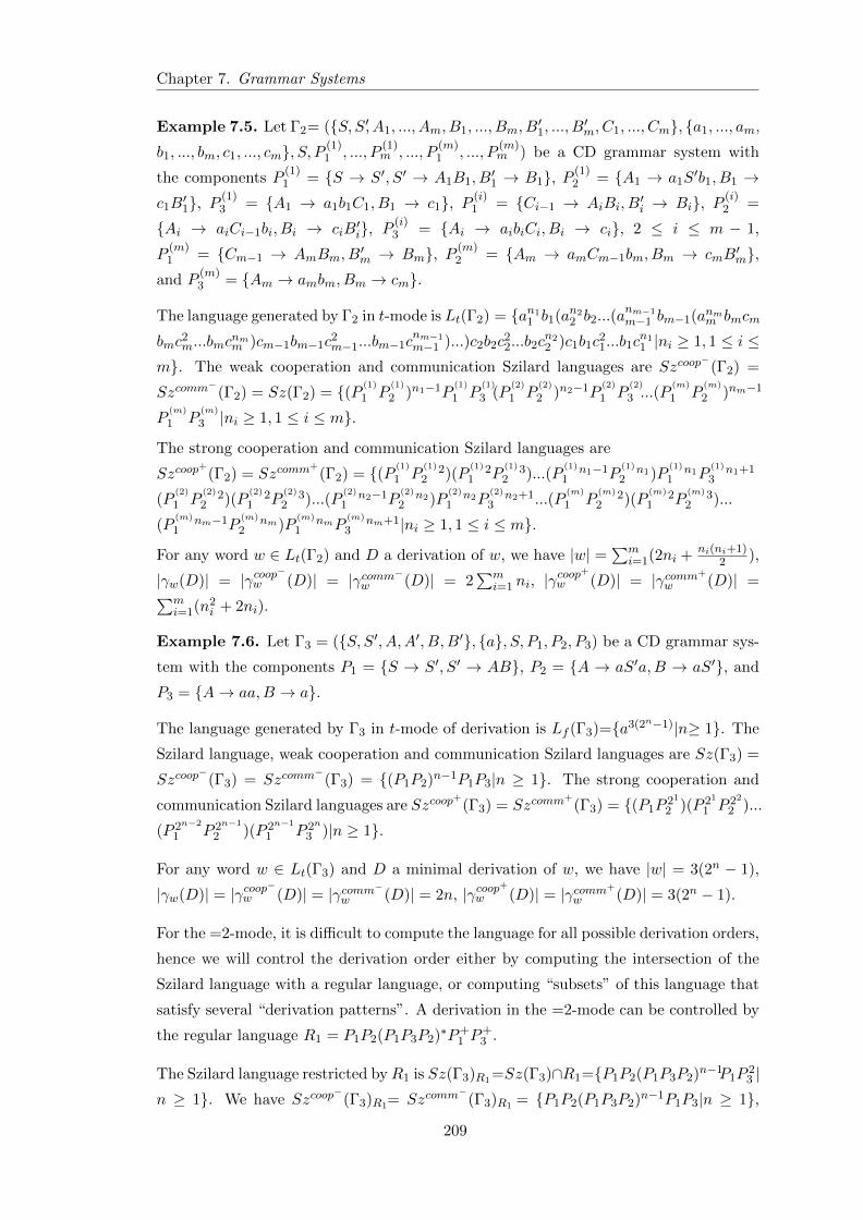
Chapter 7. Grammar Systems
Example 7.5. Let Γ2= (S, S′, A1, ..., Am, B1, ..., Bm, B′1, ..., B
′m, C1, ..., Cm, a1, ..., am,
b1, ..., bm, c1, ..., cm, S, P (1)1 , ..., P
(1)m , ..., P
(m)1 , ..., P
(m)m ) be a CD grammar system with
the components P(1)1 = S → S′, S′ → A1B1, B
′1 → B1, P (1)
2 = A1 → a1S′b1, B1 →
c1B′1, P
(1)3 = A1 → a1b1C1, B1 → c1, P (i)
1 = Ci−1 → AiBi, B′i → Bi, P (i)
2 =
Ai → aiCi−1bi, Bi → ciB′i, P
(i)3 = Ai → aibiCi, Bi → ci, 2 ≤ i ≤ m − 1,
P(m)1 = Cm−1 → AmBm, B
′m → Bm, P (m)
2 = Am → amCm−1bm, Bm → cmB′m,
and P(m)3 = Am → ambm, Bm → cm.
The language generated by Γ2 in t-mode is Lt(Γ2) = an11 b1(an2
2 b2...(anm−1
m−1 bm−1(anmm bmcm
bmc2m...bmc
nmm )cm−1bm−1c
2m−1...bm−1c
nm−1
m−1 )...)c2b2c22...b2c
n22 )c1b1c
21...b1c
n11 |ni ≥ 1, 1 ≤ i ≤
m. The weak cooperation and communication Szilard languages are Szcoop−
(Γ2) =
Szcomm−
(Γ2) = Sz(Γ2) = (P (1)
1 P(1)
2 )n1−1P(1)
1 P(1)
3 (P(2)
1 P(2)
2 )n2−1P(2)
1 P(2)
3 ...(P(m)
1 P(m)
2 )nm−1
P(m)
1 P(m)
3 |ni ≥ 1, 1 ≤ i ≤ m.
The strong cooperation and communication Szilard languages are
Szcoop+
(Γ2) = Szcomm+
(Γ2) = (P (1)
1 P(1)
22)(P
(1)
12P
(1)
23)...(P
(1)
1n1−1P
(1)
2n1)P
(1)
1n1P
(1)
3n1+1
(P(2)
1 P(2)
22)(P
(2)
12P
(2)
23)...(P
(2)
1n2−1P
(2)
2n2)P
(2)
1n2P
(2)
3n2+1...(P
(m)
1 P(m)
22)(P
(m)
12P
(m)
23)...
(P(m)
1nm−1P
(m)
2nm)P
(m)
1nmP
(m)
3nm+1|ni ≥ 1, 1 ≤ i ≤ m.
For any word w ∈ Lt(Γ2) and D a derivation of w, we have |w| =∑m
i=1(2ni + ni(ni+1)2 ),
|γw(D)| = |γcoop−
w (D)| = |γcomm−w (D)| = 2∑m
i=1 ni, |γcoop+
w (D)| = |γcomm+
w (D)| =∑mi=1(n2
i + 2ni).
Example 7.6. Let Γ3 = (S, S′, A,A′, B,B′, a, S, P1, P2, P3) be a CD grammar sys-
tem with the components P1 = S → S′, S′ → AB, P2 = A → aS′a,B → aS′, and
P3 = A→ aa,B → a.
The language generated by Γ3 in t-mode of derivation is Lf (Γ3)=a3(2n−1)|n≥ 1. The
Szilard language, weak cooperation and communication Szilard languages are Sz(Γ3) =
Szcoop−
(Γ3) = Szcomm−
(Γ3) = (P1P2)n−1P1P3|n ≥ 1. The strong cooperation and
communication Szilard languages are Szcoop+
(Γ3) = Szcomm+
(Γ3) = (P1P21
2 )(P 21
1 P 22
2 )...
(P 2n−2
1 P 2n−1
2 )(P 2n−1
1 P 2n3 )|n ≥ 1.
For any word w ∈ Lt(Γ3) and D a minimal derivation of w, we have |w| = 3(2n − 1),
|γw(D)| = |γcoop−
w (D)| = |γcomm−w (D)| = 2n, |γcoop+
w (D)| = |γcomm+
w (D)| = 3(2n − 1).
For the =2-mode, it is difficult to compute the language for all possible derivation orders,
hence we will control the derivation order either by computing the intersection of the
Szilard language with a regular language, or computing “subsets” of this language that
satisfy several “derivation patterns”. A derivation in the =2-mode can be controlled by
the regular language R1 = P1P2(P1P3P2)∗P+1 P
+3 .
The Szilard language restricted byR1 is Sz(Γ3)R1=Sz(Γ3)∩R1=P1P2(P1P3P2)n−1P1P23 |
n ≥ 1. We have Szcoop−
(Γ3)R1= Szcomm−
(Γ3)R1 = P1P2(P1P3P2)n−1P1P3|n ≥ 1,
209
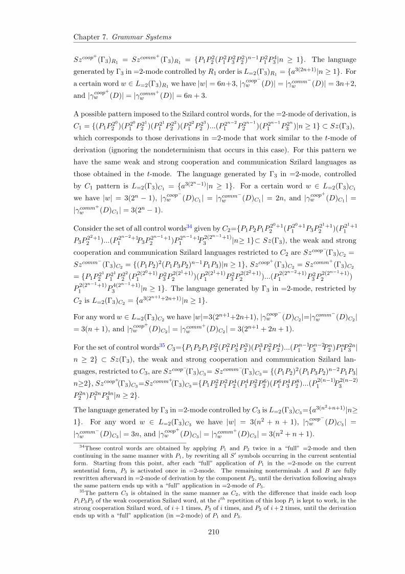
Chapter 7. Grammar Systems
Szcoop+
(Γ3)R1 = Szcomm+
(Γ3)R1 = P1P22 (P 2
1P23P
22 )n−1P 2
1P43 |n ≥ 1. The language
generated by Γ3 in =2-mode controlled by R1 order is L=2(Γ3)R1 = a3(2n+1)|n ≥ 1. For
a certain word w ∈ L=2(Γ3)R1 we have |w| = 6n+3, |γcoop−
w (D)| = |γcomm−w (D)| = 3n+2,
and |γcoop+
w (D)| = |γcomm+
w (D)| = 6n+ 3.
A possible pattern imposed to the Szilard control words, for the =2-mode of derivation, is
C1 = (P1P20
2 )(P 20
1 P 21
2 )(P 21
1 P 22
2 )(P 22
1 P 23
2 )...(P 2n−2
1 P 2n−1
2 )(P 2n−1
1 P 2n3 )|n ≥ 1 ⊂ Sz(Γ3),
which corresponds to those derivations in =2-mode that work similar to the t-mode of
derivation (ignoring the nondeterminism that occurs in this case). For this pattern we
have the same weak and strong cooperation and communication Szilard languages as
those obtained in the t-mode. The language generated by Γ3 in =2-mode, controlled
by C1 pattern is L=2(Γ3)C1 = a3(2n−1)|n ≥ 1. For a certain word w ∈ L=2(Γ3)C1
we have |w| = 3(2n − 1), |γcoop−
w (D)C1 | = |γcomm−w (D)C1 | = 2n, and |γcoop+
w (D)C1 | =
|γcomm+
w (D)C1 | = 3(2n − 1).
Consider the set of all control words34 given by C2=P1P2P1P20+12 (P 20+1
1 P3P21+12 )(P 21+1
1
P3P22+12 )...(P 2n−2+1
1 P3P2n−1+12 )P 2n−1+1
1 P2(2n−1+1)3 |n≥ 1⊂ Sz(Γ3), the weak and strong
cooperation and communication Szilard languages restricted to C2 are Szcoop−(Γ3)C2 =
Szcomm−
(Γ3)C2 = (P1P2)2(P1P3P2)n−1P1P3)|n ≥ 1, Szcoop+(Γ3)C2 = Szcomm
+(Γ3)C2
= P1P21
2 P 21
1 P 22
2 (P2(20+1)1 P 2
3P2(21+1)2 )(P
2(21+1)1 P 2
3P2(22+1)2 )...(P
2(2n−2+1)1 P 2
3P2(2n−1+1)2 )
P2(2n−1+1)1 P
4(2n−1+1)3 |n ≥ 1. The language generated by Γ3 in =2-mode, restricted by
C2 is L=2(Γ3)C2 = a3(2n+1+2n+1)|n ≥ 1.
For any word w ∈ L=2(Γ3)C2 we have |w|=3(2n+1+2n+1), |γcoop−
w (D)C2 |=|γcomm−
w (D)C2 |= 3(n+ 1), and |γcoop
+
w (D)C2 | = |γcomm+
w (D)C2 | = 3(2n+1 + 2n+ 1).
For the set of control words35 C3=P1P2P1P22 (P 2
1P13P
32 )(P 3
1P23P
42 )...(Pn−1
1 Pn−23 Pn2 )Pn1P
2n3 |
n ≥ 2 ⊂ Sz(Γ3), the weak and strong cooperation and communication Szilard lan-
guages, restricted to C3, are Szcoop−(Γ3)C3= Szcomm
−(Γ3)C3= (P1P2)2(P1P3P2)n−2P1P3|
n≥2, Szcoop+(Γ3)C3=Szcomm
+(Γ3)C3=P1P
22P
21P
42 (P 4
1P23P
62 )(P 6
1P43P
82 )...(P
2(n−1)1 P
2(n−2)3
P 2n2 )P 2n
1 P 4n3 |n ≥ 2.
The language generated by Γ3 in =2-mode controlled by C3 is L=2(Γ3)C3=a3(n2+n+1)|n≥1. For any word w ∈ L=2(Γ3)C3 we have |w| = 3(n2 + n + 1), |γcoop
−w (D)C3 | =
|γcomm−w (D)C3 | = 3n, and |γcoop+
w (D)C3 | = |γcomm+
w (D)C3 | = 3(n2 + n+ 1).
34These control words are obtained by applying P1 and P2 twice in a “full” =2-mode and thencontinuing in the same manner with P1, by rewriting all S′ symbols occurring in the current sententialform. Starting from this point, after each “full” application of P1 in the =2-mode on the currentsentential form, P3 is activated once in =2-mode. The remaining nonterminals A and B are fullyrewritten afterward in =2-mode of derivation by the component P2, until the derivation following alwaysthe same pattern ends up with a “full” application in =2-mode of P3.
35The pattern C3 is obtained in the same manner as C2, with the difference that inside each loopP1P3P2 of the weak cooperation Szilard word, at the ith repetition of this loop P1 is kept to work, in thestrong cooperation Szilard word, of i+ 1 times, P3 of i times, and P2 of i+ 2 times, until the derivationends up with a “full” application (in =2-mode) of P1 and P3.
210
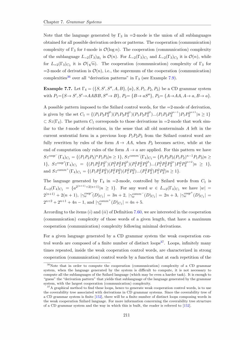
Chapter 7. Grammar Systems
Note that the language generated by Γ3 in =2-mode is the union of all sublanguages
obtained for all possible derivation orders or patterns. The cooperation (communication)
complexity of Γ3 for t-mode is O(log n). The cooperation (communication) complexity
of the sublanguage L=2(Γ3)R1 is O(n). For L=2(Γ3)C1 and L=2(Γ3)C2 it is O(n), while
for L=2(Γ3)C3 it is O(√n). The cooperation (communication) complexity of Γ3 for
=2-mode of derivation is O(n), i.e., the supremum of the cooperation (communication)
complexities36 over all “derivation patterns” in Γ3 (see Example 7.9).
Example 7.7. Let Γ4 = (S, S′, S′′, A,B, a, S, P1, P2, P3) be a CD grammar system
with P1=S→ S′, S′→AABB,S′′→ B, P2= B→ aS′′, P3= A→AA,A→ a,B→ a.
A possible pattern imposed to the Szilard control words, for the =2-mode of derivation,
is given by the set C1 = (P1P2P20
3 )(P1P2P21
3 )(P1P2P22
3 )...(P1P2P2n−1
3 )P1P2n+1
3 |n ≥ 1⊂ Sz(Γ4). The pattern C1 corresponds to those derivations in =2-mode that work sim-
ilar to the t-mode of derivation, in the sense that all old nonterminals A left in the
current sentential form in a previous loop P1P2P3 from the Szilard control word are
fully rewritten by rules of the form A→ AA, when P3 becomes active, while at the
end of computation only rules of the form A→ a are applied. For this pattern we have
Szcoop−
(Γ4)C1 = (P1P2P3)nP1P3|n ≥ 1, Szcomm−(Γ4)C1= P1P2P3(P1P2)n−1P1P3|n ≥1, Szcoop+
(Γ4)C1 = (P1P22P
21
3 )(P 21P
22P
22
3 )(P 21P
22P
23
3 )...(P 21P
22P
2n3 )P 2
1P2n+2
3 |n ≥ 1,and Szcomm
+(Γ4)C1 = (P1P
22P
23 )(P 2
1P22 )(P 2
1P22 )...(P 2
1P22 )P 2
1P23 |n ≥ 1.
The language generated by Γ4 in =2-mode, controlled by Szilard words from C1 is
L=2(Γ4)C1 = a2(n+1)+2(n+1)|n ≥ 1. For any word w ∈ L=2(Γ4)C1 we have |w| =
2(n+1) + 2(n + 1), |γcoop−
w (D)C1 | = 3n + 2, |γcomm−w (D)C1 | = 2n + 3, |γcoop+
w (D)C1 | =
2n+2 + 2n+1 + 4n− 1, and |γcomm+
w (D)C1 | = 4n+ 5.
According to the items (i) and (ii) of Definition 7.60, we are interested in the cooperation
(communication) complexity of those words of a given length, that have a maximum
cooperation (communication) complexity following minimal derivations.
For a given language generated by a CD grammar system the weak cooperation con-
trol words are composed of a finite number of distinct loops37. Loops, infinitely many
times repeated, inside the weak cooperation control words, are characterized in strong
cooperation (communication) control words by a function that at each repetition of the
36Note that in order to compute the cooperation (communication) complexity of a CD grammarsystem, when the language generated by the system is difficult to compute, it is not necessary tocompute all the sublanguages of the Szilard language (which may be even a harder task). It is enough to“guess” the “derivation pattern” that yields that sublanguage of the language generated by the grammarsystem, with the largest cooperation (communication) complexity.
37A graphical method to find these loops, hence to generate weak cooperation control words, is to usethe coverability tree associated with derivations in CD grammar systems. Since the coverability tree ofa CD grammar system is finite [152], there will be a finite number of distinct loops composing words inthe weak cooperation Szilard language. For more information concerning the coverability tree structureof a CD grammar system and the way in which this is built, the reader is referred to [152].
211
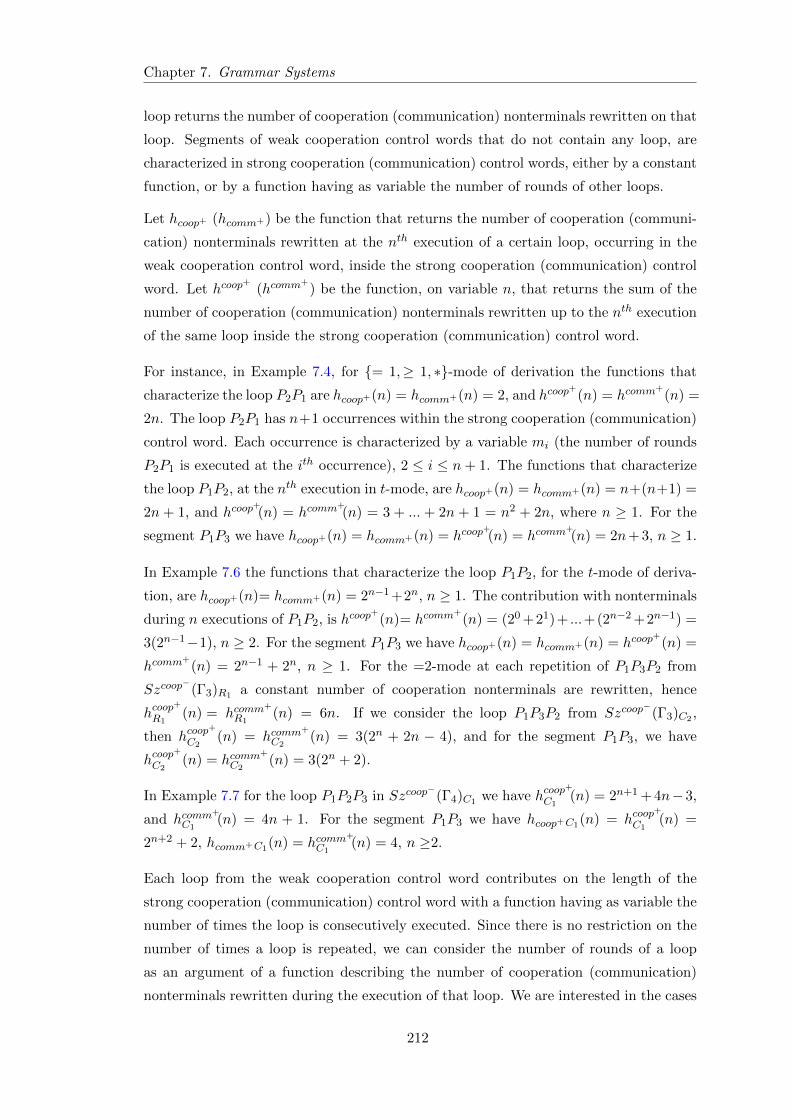
Chapter 7. Grammar Systems
loop returns the number of cooperation (communication) nonterminals rewritten on that
loop. Segments of weak cooperation control words that do not contain any loop, are
characterized in strong cooperation (communication) control words, either by a constant
function, or by a function having as variable the number of rounds of other loops.
Let hcoop+ (hcomm+) be the function that returns the number of cooperation (communi-
cation) nonterminals rewritten at the nth execution of a certain loop, occurring in the
weak cooperation control word, inside the strong cooperation (communication) control
word. Let hcoop+
(hcomm+
) be the function, on variable n, that returns the sum of the
number of cooperation (communication) nonterminals rewritten up to the nth execution
of the same loop inside the strong cooperation (communication) control word.
For instance, in Example 7.4, for = 1,≥ 1, ∗-mode of derivation the functions that
characterize the loop P2P1 are hcoop+(n) = hcomm+(n) = 2, and hcoop+
(n) = hcomm+
(n) =
2n. The loop P2P1 has n+1 occurrences within the strong cooperation (communication)
control word. Each occurrence is characterized by a variable mi (the number of rounds
P2P1 is executed at the ith occurrence), 2 ≤ i ≤ n+ 1. The functions that characterize
the loop P1P2, at the nth execution in t-mode, are hcoop+(n) = hcomm+(n) = n+(n+1) =
2n + 1, and hcoop+(n) = hcomm
+(n) = 3 + ... + 2n + 1 = n2 + 2n, where n ≥ 1. For the
segment P1P3 we have hcoop+(n) = hcomm+(n) = hcoop+(n) = hcomm
+(n) = 2n+ 3, n ≥ 1.
In Example 7.6 the functions that characterize the loop P1P2, for the t-mode of deriva-
tion, are hcoop+(n)= hcomm+(n) = 2n−1 +2n, n ≥ 1. The contribution with nonterminals
during n executions of P1P2, is hcoop+
(n)= hcomm+
(n) = (20 +21)+ ...+(2n−2 +2n−1) =
3(2n−1−1), n ≥ 2. For the segment P1P3 we have hcoop+(n) = hcomm+(n) = hcoop+
(n) =
hcomm+
(n) = 2n−1 + 2n, n ≥ 1. For the =2-mode at each repetition of P1P3P2 from
Szcoop−
(Γ3)R1 a constant number of cooperation nonterminals are rewritten, hence
hcoop+
R1(n) = hcomm
+
R1(n) = 6n. If we consider the loop P1P3P2 from Szcoop
−(Γ3)C2 ,
then hcoop+
C2(n) = hcomm
+
C2(n) = 3(2n + 2n − 4), and for the segment P1P3, we have
hcoop+
C2(n) = hcomm
+
C2(n) = 3(2n + 2).
In Example 7.7 for the loop P1P2P3 in Szcoop−
(Γ4)C1 we have hcoop+
C1(n) = 2n+1 + 4n−3,
and hcomm+
C1(n) = 4n + 1. For the segment P1P3 we have hcoop+C1(n) = hcoop
+
C1(n) =
2n+2 + 2, hcomm+C1(n) = hcomm+
C1(n) = 4, n ≥2.
Each loop from the weak cooperation control word contributes on the length of the
strong cooperation (communication) control word with a function having as variable the
number of times the loop is consecutively executed. Since there is no restriction on the
number of times a loop is repeated, we can consider the number of rounds of a loop
as an argument of a function describing the number of cooperation (communication)
nonterminals rewritten during the execution of that loop. We are interested in the cases
212
Chapter 7. Grammar Systems
where all these arguments are infinitely larger. This implies a regularity on the number
of cooperation (communication) nonterminals rewritten at each execution of a loop.
When a loop has been executed n times, the number of cooperation (communication)
nonterminals occurring in the strong cooperation (communication) control word during
the execution of that loop, becomes a function that depends on n.
For each CD grammar system working in f -mode, f ∈M , the set of all terminal (mini-
mal) derivations can be divided into several classes of derivations. Each class is composed
of those derivations in f -mode for which the weak cooperation control words have the
same structure, i.e., each γcoop−
w (D) is composed of the same loops, occurring in the
same order for each derivation D belonging to the same class.
Let Γ be a CD grammar system working in f -mode. Denote by DΓf the set of all
possible derivation classes, then |DΓf | is finite. Furthermore, each class from DΓf can be
characterized by several patterns that yield the same structure on the strong cooperation
(communication) control words (see Example 7.6).
Let Πδ be the set of all possible derivation patterns of a given class δ ∈ DΓf , and
π ∈ Πδ be an arbitrary pattern. Then by δπ we denote the subset of δ composed of all
derivations from δ restricted by the pattern π. All derivations from δπ have the property
that the words generated by these derivations can be ordered into a unique sequence
according to their lengths. The sequence defines a growth function that for each n ∈ Nreturns the length of the nth word in the sequence. More precisely, if wi, i ≥ 0, is an
infinite sequence of words, then the function f(n) = |wn|, is called the growth function
of the sequence. The notion has been introduced for deterministic systems, such as D0L
(Deterministic 0-interaction Lindenmayer) systems [184] (Subsection 6.4.1), since in the
deterministic case the lengths of words can be uniquely determined.
CD grammar systems are highly nondeterministic systems, and therefore a growth func-
tion for these systems cannot be defined. This is the reason why we classify the deriva-
tions into classes of derivations generating words that can be aligned into a growth
sequence according to their length. Each loop from the weak cooperation (communica-
tion) control word is characterized inside the corresponding strong cooperation (commu-
nication) control word associated with a derivation D belonging to a certain derivation
class, by a function having as variable the number of rounds the loop from the weak
cooperation (communication) control word is consecutively executed.
In the sequel, each minimal derivation D of w ∈ Lf (Γ), D ∈ δπ, δ ∈ DΓf , π ∈ Πδ, is
considered together with the corresponding weak and strong cooperation and commu-
nication control words, i.e., γcoop−
w (D), γcomm−
w (D), γcoop+
w (D), and γcomm+
w (D). The
structure of these elements is given by Theorem 7.72. The relations between the lengths
213
Chapter 7. Grammar Systems
of these elements, when the arguments of the functions characterizing loops occurring
in these control words tend to ∞, are presented in Lemmas 7.74 and 7.75. Based on
the limits provided in Lemmas 7.74 and 7.75, several trade-offs between time, space,
cooperation, and communication complexity measures, are provided in Corollaries 7.73
and 7.76, Theorems 7.77 and 7.79.
Theorem 7.72. (Representation Theorem) Let Γ ∈ CDGSsCF and w ∈ Lf (Γ), f ∈M .
For any minimal derivation D of w, D ∈ δπ, δ ∈ DΓf , π ∈ Πδ, and γcoop−
w (D) ∈Szcoop
−(Γ, f) with
|γcoop−w (D)| = µ+ Σd1j=1h
coop−
1,j (n1,j) + Σd2j=1h
coop−
2,j (n2,j) + ...+ Σd`j=1h
coop−
`,j (n`,j), (7.5)
where hcoop−
i,j (ni,j) = cini,j, 1≤ i ≤ `, 1≤j ≤di, there exist the sets of functions HxD,i =
hxi,jj∈1,...,di, x∈ coop+, comm−, comm+, z, w, such that hxi,j : Nxi,j→N, Nxi,j ⊆ N, and
|γxw(D)| = µx + Σd1j=1h
x1,j(n1,j) + Σd2
j=1hx2,j(n2,j) + ...+ Σd`
j=1hx`,j(nl,j), (7.6)
where 1≤ i≤`, 1≤j ≤di, γzw(D)= γw(D), γww (D)= w, ` is the finite number of distinct
loops occurring in γcoop−
w (D), ci is the number of distinct components occurring in the ith
loop38, di is the number of occurrences of the ith loop in γcoop−
w (D), ni,j is the number of
rounds of the ith loop at the jth occurrence in γcoop−
w (D), 1≤ j≤di, and µ, µx∈ O(Σ`i=1di).
Proof. Let w be an arbitrary word in Lf (Γ), f ∈M , and D a minimal derivation of w,
D ∈ δπ, δ ∈ DΓf , π ∈ Πδ. We prove the claim for γzw(D) = γw(D) and γcoop+
w (D). For
the other Szilard words the proof is similar. Suppose that γcoop−
w (D) contains ` distinct
loops39, and each of these loops may have several occurrences in γcoop−
w (D). In order to be
able to identify these loops we consider an order on the set of all distinct loops occurring
in γcoop−
w (D). Suppose that the ith loop in this ordered set is of the form Pi1 ...Pici , and at
the jth occurrence of Pi1 ...Pici in γcoop−
w (D) this loop is executed ni,j times. Furthermore,
each component in this loop works according to the derivation pattern π ∈ Πδ, obeying in
the same time the derivation f -mode. The derivation pattern π consists in a regularity
imposed on the number of times each component in Pi1 ...Pici is kept active at each
execution of the loop performed in f -mode. The number of times a component is kept
active on the sentential form can be counted within the control word40 γw(D). The
sum of the number of times all components have been applied during ni,j executions
of loop Pi1 ...Pici will be a linear, polynomial, or exponential function of ni,j . Since the
regularity imposed on the number of times each component is applied at each execution
38We consider an order on the distinct loops occurring in γcoop−
w (D), each loop being marked by aunique label i, 1 ≤ i ≤ `.
39If γcoop−
w (D) contains no loop, Lf (Γ) has constant cooperation and communication complexity.40If during a derivation step, generating a word w, a component P is applied l consecutive times in a
certain derivation mode, then the label of P is concatenated l times in γw(D).
214
Chapter 7. Grammar Systems
of Pi1 ...Pici , implies a regularity on the number of cooperation nonterminals rewritten at
each repetition of the loop, the sum of the number of cooperation nonterminals rewritten
up to the nthi,j execution of the loop Pi1 ...Pici will be a linear (Example 7.4), polynomial
(Examples 7.4 and 7.5), or exponential function of ni,j (Examples 7.6 and 7.7).
Consider the function hcoop−
i,j (ni,j) = cini,j that characterizes the loop Pi1 ...Pici in
γcoop−
w (D). With hcoop−
i,j we associate the functions hzi,j and hcoop+
i,j that respectively
provide the sum of the number of times each component in Pi1 ...Pici is activated and
the sum of the number of cooperation nonterminals rewritten, up to the nthi,j execution
of loop Pi1 ...Pici . In this way, with the ith loop characterized by the set of functions
Hcoop−
D,i = hcoop−
i,j j∈1,...,di, hcoop−
i,j (ni,j) = cini,j , where di is the number of occurrences
of the loop Pi1 ...Pici in γcoop−
w (D) and ni,j is the number of rounds of Pi1 ...Pici at the
jth occurrence of Pi1 ...Pici in γcoop−
w (D), 1 ≤ j ≤ di, we associate the set of functions
HzD,i = hzi,jj∈1,...,di and Hcoop+
D,i = hcoop+
i,j j∈1,...,di.
Besides loops, in γcoop−
w (D) there may exist segments containing no loop. The sum of the
lengths of these segments is µ ∈ O(Σ`i=1di). Inside γcoop
+
w (D), the sum of the lengths of
these segments may depend on the number of loops occurring in γcoop−
w (D), i.e., µcoop+ ∈O(Σ`
i=1di), but they may also be characterized by some functions that depend on the
number of rounds of loops occurring in γcoop−
w (D), i.e., arguments of type ni,j . In this
case each function that depends on ni,j is added to the corresponding function hcoop+
i,j of
variable ni,j . The same observation holds for µz ∈ O(Σ`i=1di).
Hence, if (7.5) gives the length of γcoop−
w (D), then by summing all functions in HxD,i =
hxi,jj∈1,...,di, where each hxi,j depends on ni,j , and the corresponding residual value µx,
we obtain, for the length of the Szilard control words γxw(D), x ∈ z, coop+, a formula
of type (7.6). If instead of cooperation nonterminals we sum the number of terminals
pumped in the sentential form up to the nthi,j execution of loop Pi1 ...Pici , we obtain a
null function (if no terminal is pumped into the sentential form), a linear, polynomial
or exponential function on ni,j . The union of these functions gives the set HwD,i =
hwi,jj∈1,...,di that characterize the ith loop of γcoop−
w (D), in γww (D) = w. The sum of
all these functions in the corresponding arguments ni,j , 1 ≤ i ≤ `, 1 ≤ j ≤ di, and the
residual value µw ∈ O(Σ`i=1di) gives the formula (7.6) for the length of γww (D) = w.
ConsiderHxD= ∪1≤i≤`HxD,i,HzD= ∪
1≤i≤`HzD,i, andHwD= ∪1≤i≤`HwD,i, x ∈coop−, coop+, comm−,
comm+.
Corollary 7.73. Let Γ ∈ CDGSsCF. For any word w ∈ Lf (Γ), and D a minimal deriva-
tion of w in f -mode, f ∈M , we have either |γcoop−
w (D)| = O(|γcoop+
w (D)|), |γcoop−
w (D)| =
O(k
√|γcoop
+
w (D)|), or |γcoop−
w (D)| = O(log(|γcoop+
w (D)|)).
215
Chapter 7. Grammar Systems
Proof. If Hcoop+
D contains at least one exponential function, then from (7.5) and (7.6) we
have |γcoop−
w (D)| = log(2µ)+log(2Σd1j=1c1n1,j )+ ...+log(2Σ
d`j=1c`n`,j ) = O(log(|γcoop
+
w (D)|)).If there exists at least one polynomial function and no exponential function in Hcoop
+
D ,
then |γcoop−
w (D)|=O(k
√|γcoop
+
w (D)|), k ≥ 2. If Hcoop+
D contains only linear functions, then
|γcoop−
w (D)|= O(|γcoop+
w (D)|).
By Theorem 7.72 we divide the computation into several “loops” of computation, and
we compute the cooperation (communication) complexity at the level of each loop. The
cooperation (communication) complexity of the whole computation, for a certain word
w and a minimal derivation D of w, will be the sum of the cooperation (communication)
complexities of all loops inside the cooperation (communication) Szilard word. The
cooperation (communication) complexity of the whole language will be considered as the
maximum of the cooperation (communication) complexity over all possible derivations
of words in the language. Next, we give an example that deals with this idea.
Example 7.8. Let Lt(Γ1) = anbcbc2...bcn|n ≥ 1 be the language generated by Γ1
in Example 7.4, in t-mode. For any word w ∈ Lt(Γ1) of length |w| = 12(n2 + 5n),
n ≥ 1, we have |γcoop−
w (D)| = |γcomm−w (D)| = 2n, and |γcoop+
w (D)| = |γcomm+
w (D)| =
hcoop+
P1P2(n) + hcoop
+
P1P3(n) = hcomm
+
P1P2(n) + hcomm
+
P1P3(n) = n2 − 1 + 2n + 1 = n2 + 2n, where
hcoop+
P1P2(n) = hcomm
+
P1P2(n) = n2 − 1 and hcoop
+
P1P3(n) = hcomm
+
P1P3(n) = 2n + 1 are the func-
tions that characterize the loop P1P2 and the segment P1P3, respectively. Furthermore,
we have |γcoop−
w (D)| = |γcomm−w (D)| = 2n = 2√n2 ≤ 2
√n2 + 2n = 2
√γcoop
+
w (D) =
2√γcomm+
w (D) =O(√|w|). Hence, CoopΓ1(n) = CommΓ1(n) = supCoop(w,Γ1)|w ∈
Lf (Γ1), |w| = n = O(√n).
Note that if the component P2 in Example 7.4 is replaced by P ′2 = A → S′, B → B′,we have Coop
Γ′1(n) = Comm
Γ′1(n) = supCoop(w,Γ′1)|w ∈ Lf (Γ
′1), |w| = n = O(n).
Example 7.9. Consider the CD grammar system in Example 7.6. The language re-
stricted to the derivation pattern C2, for the =2-mode of derivation, is L=2(Γ3)C2 =
a3(2n+1+2n+1)|n ≥ 1. Any word w ∈ L=2(Γ3)C2 of length |w| = 3(2n+1 + 2n + 1),
n ≥ 1, has the corresponding weak cooperation control word of length |γcoop−
w (D)C2 | =3(n + 1). The strong cooperation and communication control words have the length
|γcoop+
w C2(D)| = |γcomm+
w C2(D)| = hcoop+
P1P2(n) + hcoop
+
P1P3P2(n) + hcoop
+
P1P3(n) = hcomm
+
P1P2(n) +
hcomm+
P1P3P2(n) + hcomm
+
P1P3(n) = 9 + 3(2n + 2n − 4) + 3(2n + 2) = 3(2n+1 + 2n + 1), where
hcoop+
P1P2(n) = hcomm
+
P1P2(n) = 9, hcoop
+
P1P3P2(n) = hcomm
+
P1P3P2(n) = 3(2n + 2n− 4), and hcoop
+
P1P3(n) =
hcomm+
P1P3(n) = 3(2n + 2) are the functions that characterize the segment P1P2, the loop
P1P3P2, and the segment P1P3, respectively.
We have |γcoop−
w (D)C2 | = 3n+ 3 = 3 log(2n) + 3 ≤ 3 log(3(2n + 2n− 4)) ≤ 3 log(3(2n+1 +
2n + 1)) = O(log(|w|)). Hence, the cooperation and communication complexity of all
216

Chapter 7. Grammar Systems
derivations controlled by C2 are CoopΓ3(n)C2 = CommΓ3(n)C2= supCoop(w,Γ3)|w ∈Lf (Γ3)C2 , |w|= n =O(log(|w|))=O(log(n)). Analogously, CommΓ3(n)R1=CoopΓ3(n)R1
= supCoop(w,Γ3)|w ∈ Lf (Γ3)R1 , |w| = n = O(|w|) = O(n), and CoopΓ3(n)C3 =
supCoop(w,Γ3)|w ∈ Lf (Γ3)C3 , |w| = n = O(√|w|) = O(
√n). By Definition 7.60,
CommΓ3(n) = CoopΓ3(n) = supCoop(w,Γ3)|w ∈ Lf (Γ3), |w| = n = O(|w|) = O(n).
Example 7.10. For the CD grammar system Γ2, in Example 7.5, we have Lt(Γ2) =
an11 b1(an2
2 b2 (...(anm−1
m−1 bm−1 (anmm bmcmbmc2m...bmc
nmm ) cm−1bm−1c
2m−1...bm−1c
nm−1
m−1 )...)c2
b2c22...b2c
n22 ) c1b1c
21...b1c
n11 |ni ≥ 1, 1 ≤ i ≤ m. For any word w ∈ Lt(Γ2) of length |w| =∑m
i=1(2ni+ni(ni+1)
2 ) we have |γxw(D)| =∑m
i=1(n2i + 2ni), |γcoop
−w (D)| = |γcomm−w (D)| =
2∑m
i=1 ni, ni≥ 1, 1≤i ≤ m, x∈ comm+, coop+. The set of characterization functions
associated with γxw(D) is HxP
(i)1
P (i)2
= hxP
(i)1
P (i)2
1≤i≤m, hxP
(i)1
P (i)2
= n2i −1, and Hx
P(i)1
P (i)3
=
hxP
(i)1
P (i)3
1≤i≤m, hxP
(i)1
P (i)3
= 2ni + 1, x ∈ comm+, coop+. Using a similar procedure as
in Example 7.8 we have |γcoop−
w (D)| = |γcomm−w (D)| =∑m
i=12ni =∑m
i=12√n2i≤ c
√∑mi=1 n
2i
≤ c√∑m
i=1(n2i + 2ni) = c
√γcoop
+
w (D) = c√γcomm+
w (D) = O(√|w|). Hence, CoopΓ2(n) =
CommΓ2(n) = supCoop(w,Γ2)|w ∈ Lf (Γ2), |w| = n = O(√n).
In order to find trade-offs between the lengths of the weak and strong cooperation and
communication Szilard words, we consider limit operations on functions of multiple
variables. The relations between the lengths of these elements, when the arguments ni,j ,
1 ≤ j ≤ di, 1 ≤ i ≤ `, provided by the Representation Theorem 7.72, tend to ∞, are
presented in Lemmas 7.74 and 7.75.
Lemma 7.74. Let Γ be an arbitrary CD grammar system with non-erasing rules, such
that there is no component of Γ composed of only chain41 rules. Let w ∈ Lf (Γ), f ∈M ,
and D a minimal derivation of w performed in f -mode, with D ∈ δπ, δ ∈ DΓf , π ∈Πδ, and Coop(D) = |γcoop
−w (D)| = µ+ Σ`
i=1Σdij=1h
coop−
i,j (ni,j), where hcoop−
i,j (ni,j) = cini,j,
1 ≤ i ≤ `, 1 ≤ j ≤ di, ` is the finite number of distinct loops occurring in γcoop−
w (D),
and ci is the number of distinct components in the ith loop. The next limits42 hold
limni,j→∞
Comm(D)
Coop(D)= lim
ni,j→∞
|γcomm−w (D)||γcoop
−w (D)|
= ai,j , limni,j→∞
|γcomm+
w (D)||γcoop
+
w (D)|= Ai,j ,
where 0 < ai,j <∞, 0 ≤ Ai,j <∞, are constants that depend on the derivation patternπ ∈ Πδ, for any f -mode of derivation, f ∈ M . Moreover, Ai,j = 1 in t-mode, and
Ai,j ≥ 0, for f ∈M − t, for any 1 ≤ i ≤ `, 1 ≤ j ≤ di.41By not allowing “null” components, composed of only chain rules, each component brings contribu-
tions on the generated word either directly through terminal symbols (in the case of regular and linearrules), or indirectly through nonterminal symbols, that later on in the computation have to be rewritten,through other nonterminal symbols, into terminal symbols.
42All limits in Lemmas 7.74 and 7.75 are considered over a single variable. If ni,j tends to ∞, all theother variables are considered constant.
217
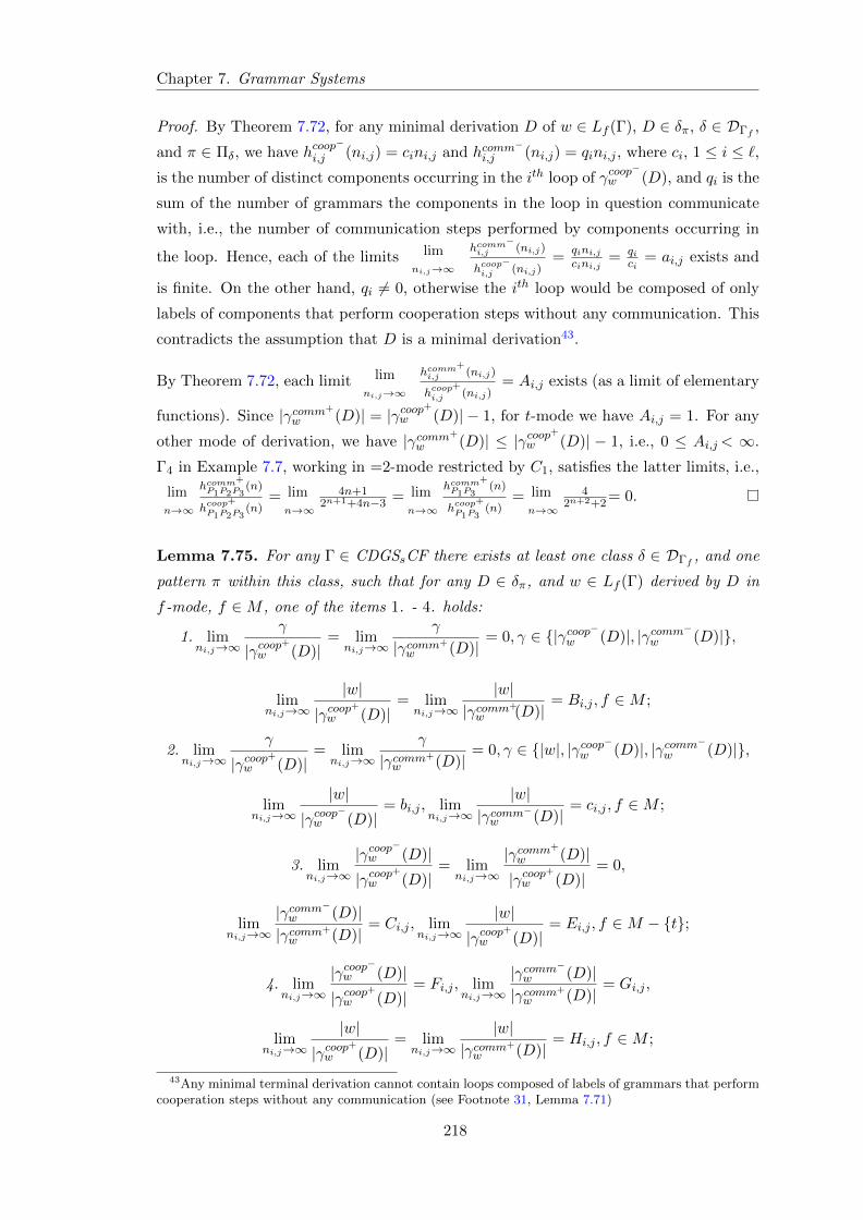
Chapter 7. Grammar Systems
Proof. By Theorem 7.72, for any minimal derivation D of w ∈ Lf (Γ), D ∈ δπ, δ ∈ DΓf ,
and π ∈ Πδ, we have hcoop−
i,j (ni,j) = cini,j and hcomm−
i,j (ni,j) = qini,j , where ci, 1 ≤ i ≤ `,is the number of distinct components occurring in the ith loop of γcoop
−w (D), and qi is the
sum of the number of grammars the components in the loop in question communicate
with, i.e., the number of communication steps performed by components occurring in
the loop. Hence, each of the limits limni,j→∞
hcomm−
i,j (ni,j)
hcoop−
i,j (ni,j)=
qini,jcini,j
= qici
= ai,j exists and
is finite. On the other hand, qi 6= 0, otherwise the ith loop would be composed of only
labels of components that perform cooperation steps without any communication. This
contradicts the assumption that D is a minimal derivation43.
By Theorem 7.72, each limit limni,j→∞
hcomm+
i,j (ni,j)
hcoop+
i,j (ni,j)= Ai,j exists (as a limit of elementary
functions). Since |γcomm+
w (D)| = |γcoop+
w (D)| − 1, for t-mode we have Ai,j = 1. For any
other mode of derivation, we have |γcomm+
w (D)| ≤ |γcoop+
w (D)| − 1, i.e., 0 ≤ Ai,j< ∞.
Γ4 in Example 7.7, working in =2-mode restricted by C1, satisfies the latter limits, i.e.,
limn→∞
hcomm+
P1P2P3(n)
hcoop+
P1P2P3(n)
= limn→∞
4n+12n+1+4n−3
= limn→∞
hcomm+
P1P3(n)
hcoop+
P1P3(n)
= limn→∞
42n+2+2
= 0.
Lemma 7.75. For any Γ ∈ CDGSsCF there exists at least one class δ ∈ DΓf , and one
pattern π within this class, such that for any D ∈ δπ, and w ∈ Lf (Γ) derived by D in
f -mode, f ∈M , one of the items 1. - 4. holds:
1. limni,j→∞
γ
|γcoop+
w (D)|= lim
ni,j→∞
γ
|γcomm+
w (D)|= 0, γ ∈ |γcoop−w (D)|, |γcomm−w (D)|,
limni,j→∞
|w||γcoop
+
w (D)|= lim
ni,j→∞
|w||γcomm+
w (D)|= Bi,j , f ∈M ;
2. limni,j→∞
γ
|γcoop+
w (D)|= lim
ni,j→∞
γ
|γcomm+
w (D)|= 0, γ ∈ |w|, |γcoop−w (D)|, |γcomm−w (D)|,
limni,j→∞
|w||γcoop
−w (D)|
= bi,j , limni,j→∞
|w||γcomm−w (D)|
= ci,j , f ∈M ;
3. limni,j→∞
|γcoop−
w (D)||γcoop
+
w (D)|= lim
ni,j→∞
|γcomm+
w (D)||γcoop
+
w (D)|= 0,
limni,j→∞
|γcomm−w (D)||γcomm+
w (D)|= Ci,j , lim
ni,j→∞
|w||γcoop
+
w (D)|= Ei,j , f ∈M − t;
4. limni,j→∞
|γcoop−
w (D)||γcoop
+
w (D)|= Fi,j , lim
ni,j→∞
|γcomm−w (D)||γcomm+
w (D)|= Gi,j ,
limni,j→∞
|w||γcoop
+
w (D)|= lim
ni,j→∞
|w||γcomm+
w (D)|= Hi,j , f ∈M ;
43Any minimal terminal derivation cannot contain loops composed of labels of grammars that performcooperation steps without any communication (see Footnote 31, Lemma 7.71)
218

Chapter 7. Grammar Systems
where Coop(D) = |γcoop−
w (D)| = µ + Σ`i=1Σdi
j=1hi,j(ni,j), is provided by Theorem 7.72,
and 0 ≤ xi,j , Xi,j < ∞, x ∈ b, c, X ∈ B,C,E, F,G,H, are constants that depend
on the derivation class and patterns, for any 1 ≤ i ≤ `, 1 ≤ j ≤ di. There exists Γ ∈CDGSsCF such that at least two of the cases 1.-4. hold true inside Γ, either for different
classes of derivations, or for the same class but for different patterns.
Proof. By Theorem 7.72 for any minimal derivation D ∈ δπ of w ∈ Lf (Γ), δ ∈ DΓf ,
π ∈ Πδ, each of the limits limni,j→∞
hcoop−
i,j (ni,j)
hcoop+
i,j (ni,j), limni,j→∞
hcomm−
i,j (ni,j)
hcomm+
i,j (ni,j), limni,j→∞
hwi,j(ni,j)
hcoop+
i,j (ni,j),
limni,j→∞
hwi,j(ni,j)
hcomm+
i,j (ni,j), limni,j→∞
hcomm+
i,j (ni,j)
hcoop+
i,j (ni,j), etc., 1 ≤ i ≤ `, 1 ≤ j ≤ di, exists.
The limits in items 1. - 4. depend on the given CD grammar system. Item 1. holds for
any CD grammar system Γ, for which there exist at least one class of derivation δ and
at least one pattern π within this class, such that for each D ∈ δπ at least one function
hcoop+
i,j ∈ Hcoop+
D,i , 1 ≤ i ≤ `, 1 ≤ j ≤ di, is at least polynomial. At each cooperation
nonterminal rewritten during the execution of the loop characterized by hcoop+
i,j , at least
one terminal is inserted into the sentential form, i.e., hwi,j and hcoop+
i,j are functions of the
same type (polynomial or exponential). The other functions hwi′,j′ , i 6= i′, j 6= j′, may
be either null, or at most of the same type with hcoop+
i′,j′ . Furthermore, Γ can be modeled
such that each cooperation nonterminal rewritten during the execution of a loop, is
also a communication nonterminal. Under these assumptions, we have 0 ≤ Bi,j < ∞,
1 ≤ i ≤ `, 1 ≤ j ≤ di. If any rule in Γ that rewrites a cooperation nonterminal
produces in the sentential form at least one terminal symbol, then 0 < Bi,j < ∞. The
derivations from Example 7.6, performed in =2-mode according with C1 pattern, satisfy
item 1., i.e., limn→∞
hcoop−
P1P2(n)
hcoop+
P1P2(n)
= limn→∞
2(n−1)3(2n−1−1)
= limn→∞
hcoop−
P1P3(n)
hcoop+
P1P3(n)
= limn→∞
22n+2n−1 = 0,
limn→∞
hwP1P2(n)
hcoop+
P1P2(n)
= limn→∞
3(2n−1−1)3(2n−1−1)
= limn→∞
hwP1P3(n)
hcoop+
P1P3(n)
= limn→∞
3·2n−1
2n+2n−1 = 1.
To prove item 2. we consider a CD grammar system for which there exist at least one
class of derivation δ and at least one pattern π within δ class, such that for each D ∈ δπat least one function hxi,j ∈ HxD,i, 1 ≤ i ≤ `, 1 ≤ j ≤ di, x ∈ coop+, comm+ is at least
polynomial, and all hwi,j , 1 ≤ i ≤ `, 1 ≤ j ≤ di, are at most linear. Under the above
assumptions 0 ≤ bi,j , ci,j < ∞, 1 ≤ i ≤ `, 1 ≤ j ≤ di. If in Example 7.4 we replace P2
by P ′2 = A→ S′, B → B′, then for t-mode all limits in item 2. hold.
For item 3. it is enough to build a CD grammar system for which there exist at least
one class of derivation δ and at least one pattern within this class π, such that for each
D ∈ δπ, any function hcomm+
i,j ∈ Hcomm+
D,i , 1 ≤ i ≤ `, 1 ≤ j ≤ di, is at most linear, and
there exists at least one polynomial function hcoop+
i,j ∈ Hcoop+
D,i , 1 ≤ i ≤ `, 1 ≤ j ≤ di.
Furthermore, there must exist at least one function hwi,j ∈ HwD,i, 1 ≤ i ≤ `, 1 ≤ j ≤ di, of
the same type with the corresponding hcoop+
i,j , and all the other functions hwi′,j′ are either
219
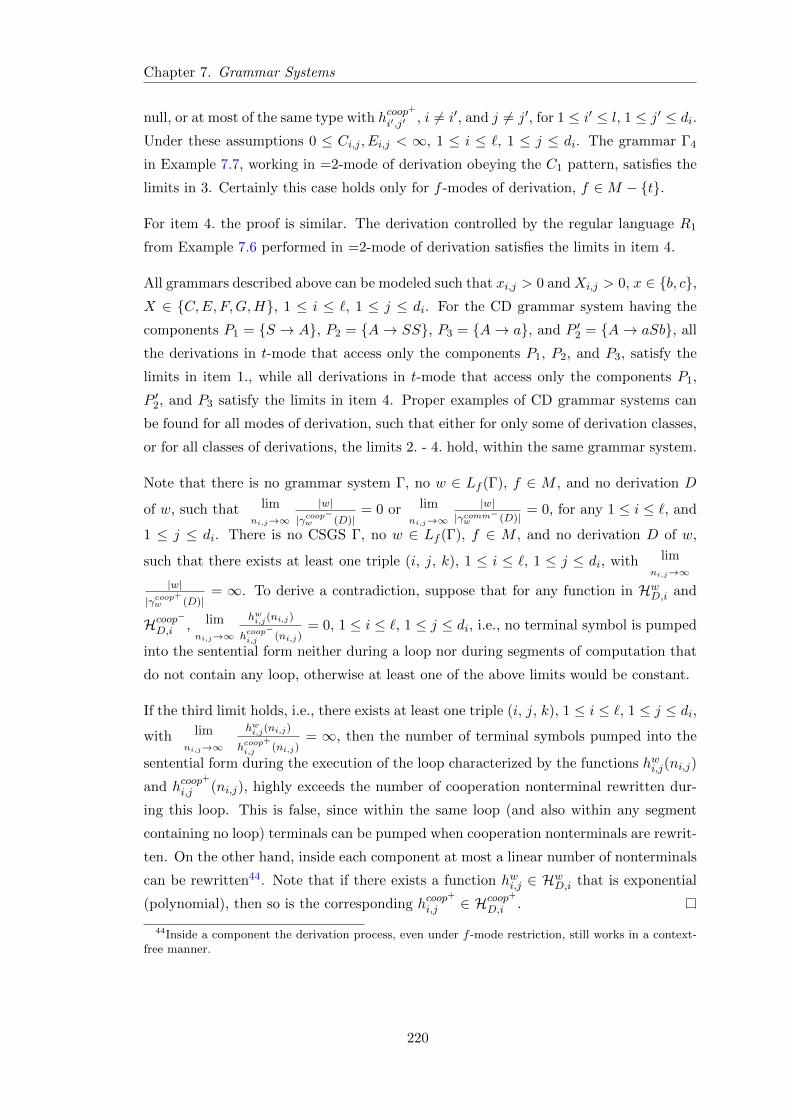
Chapter 7. Grammar Systems
null, or at most of the same type with hcoop+
i′,j′ , i 6= i′, and j 6= j′, for 1 ≤ i′ ≤ l, 1 ≤ j′ ≤ di.Under these assumptions 0 ≤ Ci,j , Ei,j < ∞, 1 ≤ i ≤ `, 1 ≤ j ≤ di. The grammar Γ4
in Example 7.7, working in =2-mode of derivation obeying the C1 pattern, satisfies the
limits in 3. Certainly this case holds only for f -modes of derivation, f ∈M − t.
For item 4. the proof is similar. The derivation controlled by the regular language R1
from Example 7.6 performed in =2-mode of derivation satisfies the limits in item 4.
All grammars described above can be modeled such that xi,j > 0 and Xi,j > 0, x ∈ b, c,X ∈ C,E, F,G,H, 1 ≤ i ≤ `, 1 ≤ j ≤ di. For the CD grammar system having the
components P1 = S → A, P2 = A→ SS, P3 = A→ a, and P ′2 = A→ aSb, all
the derivations in t-mode that access only the components P1, P2, and P3, satisfy the
limits in item 1., while all derivations in t-mode that access only the components P1,
P ′2, and P3 satisfy the limits in item 4. Proper examples of CD grammar systems can
be found for all modes of derivation, such that either for only some of derivation classes,
or for all classes of derivations, the limits 2. - 4. hold, within the same grammar system.
Note that there is no grammar system Γ, no w ∈ Lf (Γ), f ∈ M , and no derivation D
of w, such that limni,j→∞
|w||γcoop
−w (D)|
= 0 or limni,j→∞
|w||γcomm−w (D)|
= 0, for any 1 ≤ i ≤ `, and
1 ≤ j ≤ di. There is no CSGS Γ, no w ∈ Lf (Γ), f ∈ M , and no derivation D of w,
such that there exists at least one triple (i, j, k), 1 ≤ i ≤ `, 1 ≤ j ≤ di, with limni,j→∞
|w||γcoop
+w (D)|
= ∞. To derive a contradiction, suppose that for any function in HwD,i and
Hcoop−
D,i , limni,j→∞
hwi,j(ni,j)
hcoop−
i,j (ni,j)= 0, 1 ≤ i ≤ `, 1 ≤ j ≤ di, i.e., no terminal symbol is pumped
into the sentential form neither during a loop nor during segments of computation that
do not contain any loop, otherwise at least one of the above limits would be constant.
If the third limit holds, i.e., there exists at least one triple (i, j, k), 1 ≤ i ≤ `, 1 ≤ j ≤ di,
with limni,j→∞
hwi,j(ni,j)
hcoop+
i,j (ni,j)= ∞, then the number of terminal symbols pumped into the
sentential form during the execution of the loop characterized by the functions hwi,j(ni,j)
and hcoop+
i,j (ni,j), highly exceeds the number of cooperation nonterminal rewritten dur-
ing this loop. This is false, since within the same loop (and also within any segment
containing no loop) terminals can be pumped when cooperation nonterminals are rewrit-
ten. On the other hand, inside each component at most a linear number of nonterminals
can be rewritten44. Note that if there exists a function hwi,j ∈ HwD,i that is exponential
(polynomial), then so is the corresponding hcoop+
i,j ∈ Hcoop+
D,i .
44Inside a component the derivation process, even under f -mode restriction, still works in a context-free manner.
220
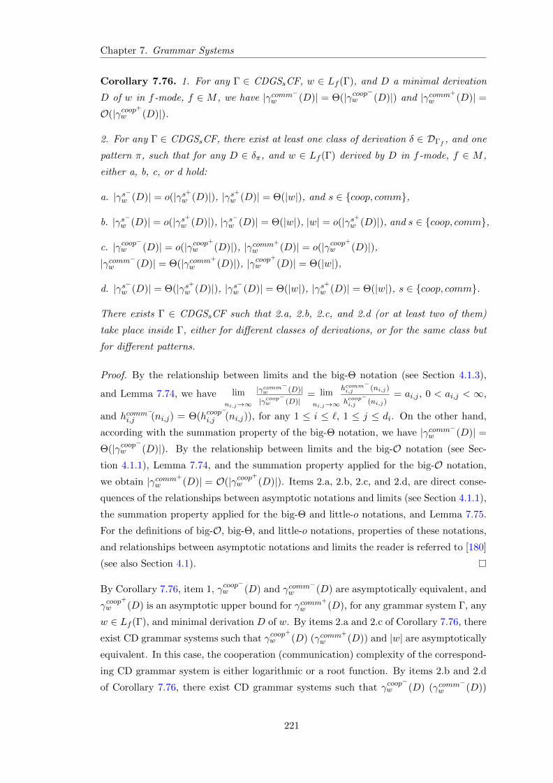
Chapter 7. Grammar Systems
Corollary 7.76. 1. For any Γ ∈ CDGSsCF, w ∈ Lf (Γ), and D a minimal derivation
D of w in f -mode, f ∈ M , we have |γcomm−w (D)| = Θ(|γcoop−
w (D)|) and |γcomm+
w (D)| =O(|γcoop
+
w (D)|).
2. For any Γ ∈ CDGSsCF, there exist at least one class of derivation δ ∈ DΓf , and one
pattern π, such that for any D ∈ δπ, and w ∈ Lf (Γ) derived by D in f -mode, f ∈ M ,
either a, b, c, or d hold:
a. |γs−w (D)| = o(|γs+w (D)|), |γs+w (D)| = Θ(|w|), and s ∈ coop, comm,
b. |γs−w (D)| = o(|γs+w (D)|), |γs−w (D)| = Θ(|w|), |w| = o(|γs+w (D)|), and s ∈ coop, comm,
c. |γcoop−
w (D)| = o(|γcoop+
w (D)|), |γcomm+
w (D)| = o(|γcoop+
w (D)|),|γcomm−w (D)| = Θ(|γcomm+
w (D)|), |γcoop+
w (D)| = Θ(|w|),
d. |γs−w (D)| = Θ(|γs+w (D)|), |γs−w (D)| = Θ(|w|), |γs+w (D)| = Θ(|w|), s ∈ coop, comm.
There exists Γ ∈ CDGSsCF such that 2.a, 2.b, 2.c, and 2.d (or at least two of them)
take place inside Γ, either for different classes of derivations, or for the same class but
for different patterns.
Proof. By the relationship between limits and the big-Θ notation (see Section 4.1.3),
and Lemma 7.74, we have limni,j→∞
|γcomm−w (D)||γcoop
−w (D)|
= limni,j→∞
hcomm−
i,j (ni,j)
hcoop−
i,j (ni,j)= ai,j , 0 < ai,j < ∞,
and hcomm−
i,j (ni,j) = Θ(hcoop−
i,j (ni,j)), for any 1 ≤ i ≤ `, 1 ≤ j ≤ di. On the other hand,
according with the summation property of the big-Θ notation, we have |γcomm−w (D)| =Θ(|γcoop
−w (D)|). By the relationship between limits and the big-O notation (see Sec-
tion 4.1.1), Lemma 7.74, and the summation property applied for the big-O notation,
we obtain |γcomm+
w (D)| = O(|γcoop+
w (D)|). Items 2.a, 2.b, 2.c, and 2.d, are direct conse-
quences of the relationships between asymptotic notations and limits (see Section 4.1.1),
the summation property applied for the big-Θ and little-o notations, and Lemma 7.75.
For the definitions of big-O, big-Θ, and little-o notations, properties of these notations,
and relationships between asymptotic notations and limits the reader is referred to [180]
(see also Section 4.1).
By Corollary 7.76, item 1, γcoop−
w (D) and γcomm−
w (D) are asymptotically equivalent, and
γcoop+
w (D) is an asymptotic upper bound for γcomm+
w (D), for any grammar system Γ, any
w ∈ Lf (Γ), and minimal derivation D of w. By items 2.a and 2.c of Corollary 7.76, there
exist CD grammar systems such that γcoop+
w (D) (γcomm+
w (D)) and |w| are asymptotically
equivalent. In this case, the cooperation (communication) complexity of the correspond-
ing CD grammar system is either logarithmic or a root function. By items 2.b and 2.d
of Corollary 7.76, there exist CD grammar systems such that γcoop−
w (D) (γcomm−
w (D))
221
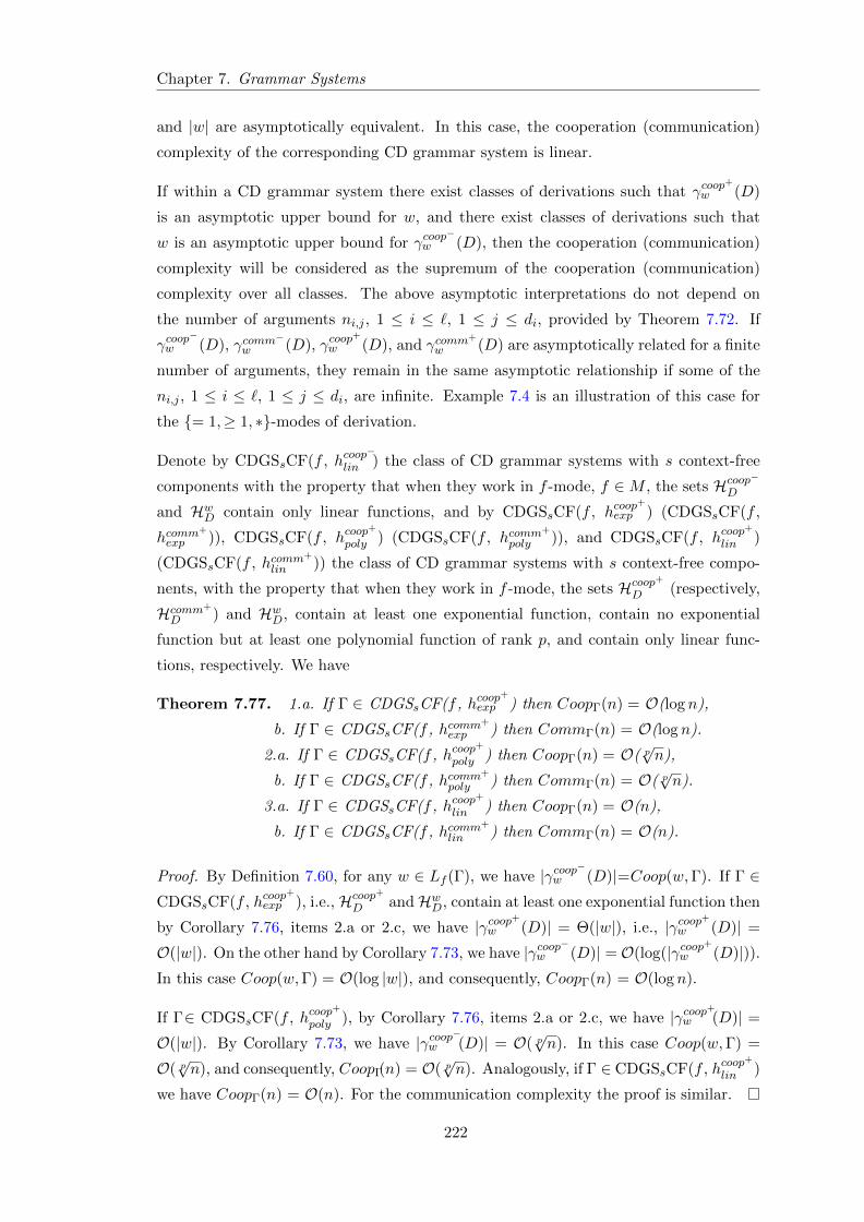
Chapter 7. Grammar Systems
and |w| are asymptotically equivalent. In this case, the cooperation (communication)
complexity of the corresponding CD grammar system is linear.
If within a CD grammar system there exist classes of derivations such that γcoop+
w (D)
is an asymptotic upper bound for w, and there exist classes of derivations such that
w is an asymptotic upper bound for γcoop−
w (D), then the cooperation (communication)
complexity will be considered as the supremum of the cooperation (communication)
complexity over all classes. The above asymptotic interpretations do not depend on
the number of arguments ni,j , 1 ≤ i ≤ `, 1 ≤ j ≤ di, provided by Theorem 7.72. If
γcoop−
w (D), γcomm−
w (D), γcoop+
w (D), and γcomm+
w (D) are asymptotically related for a finite
number of arguments, they remain in the same asymptotic relationship if some of the
ni,j , 1 ≤ i ≤ `, 1 ≤ j ≤ di, are infinite. Example 7.4 is an illustration of this case for
the = 1,≥ 1, ∗-modes of derivation.
Denote by CDGSsCF(f , hcoop−
lin ) the class of CD grammar systems with s context-free
components with the property that when they work in f -mode, f ∈M , the sets Hcoop−
D
and HwD contain only linear functions, and by CDGSsCF(f , hcoop+
exp ) (CDGSsCF(f ,
hcomm+
exp )), CDGSsCF(f , hcoop+
poly ) (CDGSsCF(f , hcomm+
poly )), and CDGSsCF(f , hcoop+
lin )
(CDGSsCF(f , hcomm+
lin )) the class of CD grammar systems with s context-free compo-
nents, with the property that when they work in f -mode, the sets Hcoop+
D (respectively,
Hcomm+
D ) and HwD, contain at least one exponential function, contain no exponential
function but at least one polynomial function of rank p, and contain only linear func-
tions, respectively. We have
Theorem 7.77. 1.a. If Γ ∈ CDGSsCF(f , hcoop+
exp ) then CoopΓ(n) = O(log n),
b. If Γ ∈ CDGSsCF(f , hcomm+
exp ) then CommΓ(n) = O(log n).
2.a. If Γ ∈ CDGSsCF(f , hcoop+
poly ) then CoopΓ(n) = O( p√n),
b. If Γ ∈ CDGSsCF(f , hcomm+
poly ) then CommΓ(n) = O( p√n).
3.a. If Γ ∈ CDGSsCF(f , hcoop+
lin ) then CoopΓ(n) = O(n),
b. If Γ ∈ CDGSsCF(f , hcomm+
lin ) then CommΓ(n) = O(n).
Proof. By Definition 7.60, for any w ∈ Lf (Γ), we have |γcoop−
w (D)|=Coop(w,Γ). If Γ ∈CDGSsCF(f , hcoop
+
exp ), i.e.,Hcoop+
D andHwD, contain at least one exponential function then
by Corollary 7.76, items 2.a or 2.c, we have |γcoop+
w (D)| = Θ(|w|), i.e., |γcoop+
w (D)| =
O(|w|). On the other hand by Corollary 7.73, we have |γcoop−
w (D)| =O(log(|γcoop+
w (D)|)).In this case Coop(w,Γ) = O(log |w|), and consequently, CoopΓ(n) = O(log n).
If Γ∈ CDGSsCF(f , hcoop+
poly ), by Corollary 7.76, items 2.a or 2.c, we have |γcoop+
w (D)| =
O(|w|). By Corollary 7.73, we have |γcoop−
w (D)| = O( p√n). In this case Coop(w,Γ) =
O( p√n), and consequently, CoopΓ(n) = O( p
√n). Analogously, if Γ ∈ CDGSsCF(f , hcoop
+
lin )
we have CoopΓ(n) = O(n). For the communication complexity the proof is similar.
222
Chapter 7. Grammar Systems
Denote by L(CDGSsCF (f, hxexp)) (L(CDGSsCF (f, hxexp, uq))), L(CDGSsCF (f, hxpoly))
(L(CDGSsCF (f, hxpoly, uq))), and L(CDGSsCF (f, hxlin)) (L(CDGSsCF (f, hxlin, uq))) the
class of languages (respectively q-fair languages) generated by CD grammar systems
in CDGSsCF(f , hxexp), CDGSsCF(f , hxpoly), and CDGSsCF(f , hxlin), u ∈ w, s, x ∈coop+, comm+, respectively. For any u ∈ w, s we have
Corollary 7.78. 1.a.L(CDGSsCF (f, hcoop+
exp ))∪L(CDGSsCF (f, hcoop+
exp , uq))⊆COOP (log n),
b. L(CDGSsCF (f, hcomm+
exp ))∪L(CDGSsCF (f, hcomm+
exp , uq)) ⊆ COMM(log n).
2.a. L(CDGSsCF (f, hcoop+
poly )) ∪ L(CDGSsCF (f, hcoop+
poly , uq)) ⊆ COOP ( p√n),
b. L(CDGSsCF (f, hcomm+
poly ))∪L(CDGSsCF (f, hcomm+
poly , uq)) ⊆ COMM( p√n).
3.a. L(CDGSsCF (f, hcoop+
lin )) ∪ L(CDGSsCF (f, hcoop+
lin , uq)) ⊆ COOP (n),
b. L(CDGSsCF (f, hcomm+
lin )) ∪ L(CDGSsCF (f, hcomm+
lin , uq)) ⊆ COMM(n).
7.2.5.4 Trade-Offs Between Time, Space, and Cooperation Complexity for
CD Grammar Systems with Context-Free Components
Next we present several trade-offs between time, space, and cooperation complexity of
languages and weakly q-fair languages generated by CD grammar systems with context-
free components.
Theorem 7.79. Let Γ = (N,T, S, P1, . . . , Ps) ∈ CDGSsCF. The languages Lf (Γ) and
Lf (Γ, wq) are accepted by a nondeterministic Turing machine T with s+m+ 2 tapes in
1. TimeT (n) = Space2T (n) = O(n2) and
i. SpaceT (n) = O(2CoopΓ(n)), if Γ ∈ CDGSsCF(f , hcoop+
exp ),
ii. SpaceT (n) = O(CooppΓ(n)), p ≥ 2, if Γ ∈ CDGSsCF(f , hcoop+
poly ),
iii. SpaceT (n) = O(CoopΓ(n)), if Γ ∈ CDGSsCF(f , hcoop+
lin ).
2. TimeT (n) = SpaceT (n) = O(2CoopΓ(n)) and CoopΓ(n) = O(n), if Γ ∈ CDGSsCF(f ,
hcoop−
lin )− CDGSsCF(f , hcoop+
lin ).
Proof. Let Γ = (N,T, S, P1, . . . , Ps) be a CD grammar system with s context-free
components such that |Pi| = ji, 1 ≤ i ≤ s. Each rule p ∈ P1 is labeled by a
unique qp, 1 ≤ qp ≤ j1, and each p ∈ Pi, 2 ≤ i ≤ s, is labeled by a unique qp,∑i−1r=1 jr + 1 ≤ qp ≤
∑ir=1 jr. We describe a nondeterministic Turing machine T with
s + m + 2 tapes, where m = |N |, that recognizes any word w ∈ Lf (Γ) ∪ Lf (Γ, wq),
f ∈ M , M = t, ∗ ∪ ≤ k,= k,≥ k|k ≥ 1. We prove the theorem for the t-mode of
derivation. For the other modes the proof is similar.
On the first tape T stores an input string w ∈ T ∗ of length n. Each tape i, 2 ≤ i ≤ s+1,
is associated with the component Pi−1 and it is composed of two tracks. The first
track stores nonterminals rewritten by Pi−1 in t-mode. Each nonterminal X is recorded
223
Chapter 7. Grammar Systems
together with a finite integer sx and two labels of types qpx and qp0 . Two other extra
cells are used for markers ∗ and ·. Hence, at most six memory cells are used by T in order
to record any X ∈ N . The second track of the ith tape is used to count cooperation
steps performed by Pi−1. Each tape i, s + 2 ≤ i ≤ s + m + 1, is associated with a
single nonterminal in N . Denote by tX the tape associated with X ∈ N . On tX , Tstores terminal strings that follow X in any rule of Γ. Some of these terminal strings
are recorded along with at most two integers of types sα and st, and two labels of types
qpα and qpt . The last tape s+m+ 2 is used to record q occurrences of $.
Briefly, T works as follows. Firstly, a prefix of w is read in the depth-first order from
the derivation tree until the very last leaf β′ ∈ T corresponding to a rule of the form
X → β, β ∈ T+, β = β′′β′
reached in this tree, is read from the input tape. Consider
those substrings wβ′aβ′b
of w, read in the depth-first order in the derivation tree, and
placed between two leaves β′a and β
′b, which correspond to rules of the form Xa → βa
and Xb → βb, βa, βb ∈ T+, such that βa = β′aβ′′a and βb = β
′′b β′b, β
′a, β
′b ∈ T . These
substrings are built on the m tapes associated with nonterminals. The order in which
they are read from these tapes and compared with substrings of w from the input tape,
is the same as the order in which nonterminals that generate them are rewritten in the
t-mode of derivation.
In details, T works as follows. Consider that any context-free rule in Γ is of the form
X → α0X1α1X2...αj−1Xjαj ...Xhαh, α0, αj ∈ T ∗, Xj ∈ N, 1 ≤ j ≤ h. (7.7)
The computation nondeterministically starts with a component Pi, 1 ≤ i≤ s, able to re-
write the axiom. Each time Pi rewrites a nonterminal X through a rule of the form (7.7)
the head i + 1 rewrites on the first track of tape i + 1 all nonterminals Xj , 1≤ j≤ h,
from the right-hand side of (7.7) that can be rewritten by Pi. All the other l+ 1 heads,
1≤ l≤ s, l 6= i, rewrite on the first track of tape l + 1 nonterminals Xj , 1≤ j≤ h, that
cannot be rewritten by Pi, but can be rewritten by Pl. Each Xj , 1≤ j≤ h, is recorded
together with the label45 qpxj associated46 with (7.7) and a finite integer sxj , 1≤ sxj≤ h,
that provides that position of Xj on the right-hand side of (7.7), i.e., sxj= j.
If more than one component Pl is able to rewrite nonterminals that cannot be rewritten
by Pi, then these nonterminals are marked on the corresponding tapes by a symbol ∗.If X is the axiom, X1 occurring in (7.7) is marked on the T ’s tape by ·. Each time a
component rewrites a nonterminal X marked by ·, already stored in the corresponding
tape of T , the first nonterminal occurring on the right-hand side of (7.7), i.e., X1, will
be also marked by ·. Each time a nonterminal X marked by · is rewritten, the string α0
45There may exist several rules that produce Xj . A marker of type qpxj makes the disambiguation.46The label of type qpx provides the label of the rule that produces the nonterminal X. The integer
sx provides the position of X on the right-hand side of rule px.
224
Chapter 7. Grammar Systems
that precedes X1 in a rule of type (7.7), is read from the input tape, without recording
it in any tape of T . If α0 cannot be read from the input tape, w is rejected.
Each nonterminal X, already stored in one of T ’s tapes, that is not marked by ·, must
be characterized by a label of type qpx , that provides the label of the rule that produced
X, and an integer sx, that provides the position of X on the right-hand side of rule px. If
sx = 1 then X is characterized by an additional label of type qp0 . When the component
Pi rewrites X, recorded on the tape i + 1 along with the above characteristics qpx , sx,
and eventually qp0 , X1 (the first nonterminal occurring on the right-hand side of the rule
that rewrites X) is recorded along with the labels qpx1and qp0 , and the integer sx1 = 1.
The label qpx1provides the label of the rule that produces X1 (and rewrites X) in the
sentential form. The label qp0 is inferred from X as follows. If X was recorded along
with a label of type qp0 then this is also the label of type qp0 of X1. If X was recorded
only with a label of type qpx , i.e., sx ≥ 2, then qp0 = qpx . Note that the label of type
qp0 is necessary in order to know on which tape associated with a nonterminal the first
terminal string α0, α0 ∈ T+, occurring on the right-hand side of the rule that rewrites
X is added to, when X is not marked by a · symbol. Next we describe the procedure
that computes qp0 for the nonterminal X.
Denote by p(1) the rule that produces X, and by X(1) the left-hand side of p(1). Suppose
that X is the j(1)th nonterminal occurring on the right-hand side of p(1), i.e., according
to notation provided in (7.7) Xj(1) = X. If j(1) ≥ 2, then qp0 = qp(1) , and α0, the first
terminal string occurring on the right-hand side of the rule that rewrites X, is added
on the tape tXj(1)−1
associated with Xj(1)−1, after the string α(1)
j(1)−1‖, where α
(1)
j(1)−1
follows Xj(1)−1 and precedes Xj(1) on the right-hand side of p(1), and ‖ is a delimiter. If
j(1) = 1, consider p(2) the rule that produces47 X(1), and X(2) the left-hand side of p(2).
Suppose that X(1) is the j(2)th nonterminal occurring on the right-hand side of p(2), i.e.,
Xj(2) = X(1). If j(2) ≥ 2 then qp0 = qp(2) , and α0 is recorded on tape tXj(2)−1
after the
string α(2)
j(2)−1‖α(1)
j(1)−1= α
(2)
j(2)−1‖α(1)
0 , already recorded on tXj(2)−1
, where α(2)
j(2)−1follows
Xj(2)−1 and precedes Xj(2) on the right-hand side of p(2). If j(2) = 1 the procedure
continues in the same manner, by searching backward in the derivation process, for
a sequence of rules p(r)p(r−1)...p(2)p(1) with the property that rule p(r−1) rewrites the
j(r)th nonterminal occurring on the right-hand side of p(r), i.e., Xj(r) , with j(r) ≥ 2,
and each rule p(q), 1 ≤ q ≤ r − 2 rewrites the very first nonterminal occurring on
the right-hand side of rule p(q+1). Then, qp0 = qp(r) and α0 is recorded on tape tXj(r)−1
after α(r)
j(r)−1‖α(r−1)
0 ...α(1)0 , already recorded on tX
j(r)−1, where α
(r)
j(r)−1follows Xj(r)−1 and
precedes Xj(r) on the right-hand side of p(r), and each α(q)0 , 1 ≤ q ≤ r − 1, is the very
first terminal string occurring on the right-hand side of rule p(q). Note that the rule p(r)
47X(1) should not have been marked by · in any tape of T . Otherwise, · is inferred by X, whichcontradicts our assumption.
225

Chapter 7. Grammar Systems
always exists, since X is not marked by ·. The marker ‖ encapsulates the information
concerning the label qpα = qp(r) of the rule that produced α(r)
j(r)−1in the sentential form,
and the position sα = j(r) − 1 of this terminal string on the right-hand side of p(r). For
the other α(q)0 , 1 ≤ q ≤ r − 2, this information is of no use.
Each αj , 1 ≤ j ≤ h, is recorded on tape tXj , associated with Xj that precedes αj in a
rule of type (7.7). It is recorded along with the label qpα of the rule that produces αj ,
and the position sα = j of αj on the right-hand side of qpα . Each αj , 1 ≤ j ≤ h, is
topped up by a symbol ]. The last terminal string occurring on the right-hand side of a
rule, i.e., αh in (7.7), is recorded on tape tXh , associated with Xh, along with the label
qpα that produces αh, and the position sα = h of αh on the right-hand side of qpα . The
string αh is also recorded along with the label of type qpt associated with the rule px
that produced X in the sentential form, i.e., qpt = qpx , and the integer st that provides
the position of X on the right-hand side of rule px, i.e., st = sx. The label qpt and
the integer st are inferred by αh from the nonterminal X, already recorded, with these
characteristics (qpx and sx) on the tape i + 1 of T . The label of type qpt is necessary
in order to know which is the rule that produced in the sentential form the string that
follows αh in the input string. After recording it, on tape tXh , αh is topped up by a
symbol ⊥. No other string can be added to αh before the ⊥ symbol, on tape tXh .
If (7.7) is a terminal rule of the form X → αt0, i.e., h = 0, then αt0 is added on tape
tXj(r)−1
, to the string α(r)
j(r)−1‖α(r−1)
0 ...α(1)0 (of which construction has been explained
above) before the ] symbol that topped up α(1)0 . Then ] is changed into ⊥ (the string is
canceled, no string can be added afterward to αt0, before ⊥). In this case, αt0 is recorded
only along with the label qpt , qpt = qpx , and the integer st, st = sx, inferred from X.
When a nonterminal is rewritten, it will be deleted (together with its characteristics)
from the tape that stored it. When a nonterminal X, marked by ∗, is rewritten one
copy of X will be deleted from all the other tapes where this has been recorded, such
that when a component, able to rewrite X, stops to work, no X will be on any tape of
T . The component Pi currently applied in t-mode, becomes idle when on the first track
of tape i+ 1 no nonterminal exists anymore. In order to mark that Pi had been applied
once during the derivation of w, the head i+ 1 writes on the second track of tape i+ 1
a symbol $. In this moment nonterminals from all l + 1 tapes, 1 ≤ l ≤ s, are the same
with the nonterminals occurring in the sentential form when Pi becomes idle.
Next T nondeterministically chooses which component continues the derivation. Con-
sider that this is the component Pk. The procedure described for component Pi is applied
in the same manner for Pk. When Pk becomes idle, the head k+ 1 writes on the second
track of tape k + 1, a symbol $ in order to mark that Pk had been applied once during
the derivation of w. The simulation continues in this way until all nonterminals from all
226
Chapter 7. Grammar Systems
tapes associated with the system components are deleted. In this moment, all strings
from tapes associated with nonterminals, are delimited only by ⊥ symbols.
The nonterminal marked by · rewritten by a rule of type Z → βt0 is kept on the tape
associated with component Pt, of whose rule rewrites Z, 1 ≤ t ≤ s, (but deleted from
other tapes on which Z may have been marked by ∗). Recall that Z was recorded on
tape t+ 1 along with the label qpz , of the rule that produced Z, and the position sz of
nonterminal Z on the right-hand side of pz.
Since T ended the simulation of Γ in t-mode, the prefix of w composed of the first termi-
nal strings occurring on the right-hand sides of rules in Γ used to rewrite nonterminals
marked by · symbols, should have been read and checked from the input tape. Denote by
β0 this prefix, whose suffix is βt0 (with the property that Z → βt0, where Z is the single
nonterminal marked by ·, kept on one of T ’s tapes associated with components). From
now on, T starts to compare strings of type βx = α(rx)
j(rx)−1α
(rx−1)0 ...α
(1)0 αt0 from tapes
associated with nonterminals with the remaining part of the input word left unchecked.
This is performed as follows.
T checks whether there exists a string of type βz on tape tZ , such that the prefix of this
string µz= α(rz)
j(rz)−1, is characterized by the label qpα= qpz and the integer sα= sz, i.e.,
µz was produced in the sentential form by the same rule pz that produced Z, in which
µz follows the sthz nonterminal occurring on the right-hand side of pz (which must be
equal with Z). Then T checks whether the string βz, delimited by two ⊥ symbols on
tape tZ , is the same with the string of length |βz| that follows β0 on the input tape. If
the two strings do not match, w is rejected. If the two strings are equal, βz is deleted
from tZ . Suppose that suffix νz = αt0 of βz is characterized by a label of type qpt and
integer st. Then T looks for the stht nonterminal occurring on the right-hand side of
rule pt. Suppose this nonterminal is Y , and α(ry)
j(ry)−1is the string that follows Y in this
rule. Then T checks whether there exists a string of type βy= α(ry)
j(ry)−1α
(ry−1)0 ...α
(1)0 αt0
on tape tY , such that the prefix of this string µy = α(ry)
j(ry)−1, is marked by label qpα ,
with qpα= qpt , and integer sα, with sα= st. If there is no string of type βy on tape tY
with this property, w is rejected. Otherwise, T checks whether string βy, delimited by
two ⊥ symbols on tape tY , is the same with the string of length |βy| that follows βz
(already checked) on input tape. If the two strings do not match, w is rejected. If the
two strings are equal, βy is deleted from tY and the procedure continues in the same
way for label qpt and integer st that characterize suffix νy= αt0 of βy. The procedure
ends when w has been entirely checked with strings of type βx from tapes associated
with nonterminals. The input w is accepted if all strings βx= α(rx)
j(rx)−1α
(rx−1)0 ...α
(1)0 αt0
are equal with substrings of w read from the input tape according to labels and integers
that characterize prefix µx= α(rx)
j(rx)−1and suffix νx= αt0 of βx.
227
Chapter 7. Grammar Systems
Note that some of βx may be of the form µx = νx = αh, where αh is the last terminal
string occurring on the right-hand side of a rule in Γ. In this case the label of type qpα
and the integer sα that provides the position of αh in the rule qpα that produces αh, is
used to make the connection between βx and the substring of w previously checked from
the input tape. The label of type qpt = qpx and integer st = sx inferred by αh from the
nonterminal X that occurs on the left-hand side of rule ppα , are used to identify on the
tapes associated with nonterminals the prefix of the next string of type βx that must be
checked with the substring of w that follows αh on the input tape.
Some of the prefixes µx and suffixes νx may be empty strings. In this case they are
recorded as empty strings, in which µx = α(rx)
j(rx)−1= λ is characterized by the label of
type qpα and48 integer sα, and νx = αt0 = λ is characterized by the label of type qpt = qpx
and49 integer sx. If w ∈ Lf (Γ), then the checking of the weak fairness conditions is
performed as in Theorem 7.67.
The space used by T to perform the computation is O(|γcoop+
w |) on tapes associated
with components, and O(|w|) on tapes associated with nonterminals. By Corollary 7.76
2.a, 2.c, and 2.d, and Theorem 7.77, we have |γcoop+
w | = Θ(|w|), i.e., |γcoop+
w | = O(|w|),case in which TimeT ∈ O(n2), SpaceT ∈ O(n), and CoopΓ ∈ O(n) if Γ ∈ CDGSsCF(f ,
hcoop+
lin ), CoopΓ ∈ O( p√n) if Γ ∈ CDGSsCF(f , hcoop
+
poly ), and CoopΓ ∈ O(log n) if Γ ∈CDGSsCF(f , hcoop
+
exp ). By Corollary 7.76, 2.b, and Theorem 7.77, we have |γcoop−
w | =
Θ(|w|), i.e., |γcoop−
w | = O(|w|), case in which TimeT = SpaceT ∈ O(2n), and CoopΓ ∈O(n), if Γ ∈ CDGSsCF(f , hcoop
−
lin )− CDGSsCF(f , hcoop+
lin ).
For the other modes of derivation T works in a similar way, with the difference that for
=1,≥1, ∗-modes of derivation T has the freedom to nondeterministically choose, at
any step of derivation, which grammar continues the derivation, no matter whether the
tape associated with grammar currently working is empty or not. For ≤ k,≥ k,=k|k ≥2-modes of derivation T has the freedom to nondeterministically choose which grammar
continues the derivation only after grammar currently active has used a number of l rules
(not necessarily distinct), where l≤ k, l ≥k, or l= modulo k, respectively. In order to
count the number of rules used by each grammar, as in Theorem 7.67, T uses at most
2k extra cells that follow the last $ recorded on tape s+m+ 2.
48Recall that qpα provides the label of the rule that “produces” α(rx)
j(rx)−1= λ, and sα provides the
position of α(rx)
j(rx)−1on the right-hand side of rule qpα .
49Recall that qpx provides the label of the rule that produces the nonterminal X placed on the left-handside of the rule that produces αt0, and sx provides the position of X in this rule.
228
Chapter 7. Grammar Systems
7.2.6 Conclusions and Further Research
In Section 7.2 we studied the communication phenomenon and the complexity of Szilard
languages of CD grammar systems that work in t, ∗ ∪ ≤ k,= k,≥ k|k ≥ 1 ∪ ≤k-comp.,= k-comp.,≥ k-comp.|k ≥ 1-modes of derivation.
In Subsection 7.2.3 we presented characterizations of CD grammar systems working in
f -mode, f ∈ ≤ k-comp.,= k-comp.,≥ k-comp.|k ≥ 1 by means of time, space and
several other resources of a multicounter machine, such as number of counters, reversals
or 0-tests. We proved that CD grammar systems working in ≤ k,= k,≥ k-competence
mode, k ≥ 1, can be simulated by one-way nondeterministic multicounter machines in
linear time and space, with a linear-bounded number of reversals (Theorem 7.41).
Imposing restrictions on the capacity of each counter to perform 0-testings, we found
that CD grammar systems working in ≤ 1,= 1 ∪ ≥ k|k ≥ 1-competence mode
can be simulated by one-way partially blind multicounter machines in quasirealtime
(Theorems 7.43 and 7.44). It is known from [90] that quasirealtime partially blind
multicounter machines accept the family of Petri net languages. Consequently, various
decision problems for partially blind multicounter machines are decidable. With respect
to them, several decidability results, for CD grammar systems working in competence
mode, grammars and systems with regulated rewriting, that emerge from the above
simulations are decidable, too. One of the most significant consequence in this respect
is that the finiteness and emptiness problems for RC-ET0L systems are decidable. This
may bring new insights in separating the L(RC,ET0L, ac) and REL classes. The results
in Subsection 7.2.3 have been published [31].
We also emphasized that the above decidability results can be also resolved via cover-
ability tree structures associated with CD grammar systems working in ≤ 1,= 1∪≥k|k ≥ 1-competence modes. The representation of CD grammar systems by means of
coverability trees and its consequences are described in [30].
In Subsection 7.2.4 we presented several simulations of CD grammar systems by bounded
width branching programs (BWBPs) (Theorems 7.47, 7.48, 7.49, 7.52, and 7.53). We
found, via BWBPs simulations of CD grammar systems working in t, ∗∪ ≤ k,= k,≥k|k ≥ 1 derivation modes, that Szilard languages associated with these systems are
included in NC1 (Theorem 7.51). Approaching CD grammar systems to BWBPs, and
consequently to NC1, gives interesting relationships between (sequential) uniform and
non-uniform models of computation (Theorems 7.52 and 7.53). Using the simulations
presented in the proofs of Theorem 7.49 and Corollary 7.50 we can think of BPs as a
good framework to obtain lower bounds on time and space complexity for CD grammar
systems. These ideas can be further developed for several other grammar systems, such
229
Chapter 7. Grammar Systems
as CD grammar systems working under competence-based protocols. The results in
Subsection 7.2.4 have been published [32].
In Subsection 7.2.5 we studied the nature of communication in CD grammar systems
working in t, ∗ ∪ ≤ k,= k,≥ k|k ≥ 1-modes of derivations that emerges from
their cooperation protocols. To attain this aim we defined several complexity structures
and two complexity measures, the cooperation and communication complexity measures
(Subsection 7.2.5.1). We presented several trade-offs between time, space, cooperation,
and communication complexity of languages generated by CD grammar systems with
regular, linear, and context-free components (Subsections 7.2.5.2 and 7.2.5.3). Coop-
eration and communication processes in CD grammar systems with regular and linear
components are of equal complexity. The two (equal) cooperation and communication
complexity measures are either constant or linear, as functions of lengths of words in the
generated language (Corollary 7.63 and Lemma 7.65). The same result holds for the co-
operation and communication complexity of q-fair languages generated by CD grammar
systems with regular and linear components (Corollary 7.64 and Theorem 7.66). For the
case of non-constant communication (cooperation) the time and space used by a nonde-
terministic multitape Turing machine to recognize weakly q-fair languages are linear, as
is the communication (cooperation) complexity (Theorem 7.67 and Corollary 7.68).
For CD grammar systems with context-free components the cooperation and commu-
nication complexity may be different. These measures vary from linear to logarithmic
functions, in terms of lengths of words in the generated language (Theorem 7.77 and
Corollary 7.78). In order to find trade-offs between time, space, cooperation, and com-
munication complexity of languages generated by CD grammar systems with context-free
components we studied asymptotic behavior of growth functions characteristic to these
measures (Corollaries 7.73 and 7.76, and Lemmas 7.74 and 7.75). We proved that lan-
guages generated by CD grammar systems with context-free components are accepted
by nondeterministic multitape Turing machines either in quadratic time, linear space,
and with cooperation complexity that varies from logarithmic to linear, or in polynomial
or exponential time and space, and linear cooperation complexity (Theorem 7.79). All
the results in Subsection 7.2.5 have been published in [34].
230
231
Bibliography
[1] S. Abraham. Some Questions of Phrase-Structure Grammars. Linguistics, 5(31):
5–12, 1967.
[2] K. Abrahamson, L. Cai, and S. Gordon. A Grammar Characterization of
Logarithmic-Space Computation. In Gh. Paun and A. Salomaa, editors, New Trends
in Formal Languages, LNCS 1218, 247–255. Springer-Verlag, 1997.
[3] M. Ajtai. A Non-Linear Time Lower Bound for Boolean Branching Programs. In
Proceedings of the 40th Annual Symposium on Foundations of Computer Science
FOCS 1999, 60–70. IEEE Computer Society, 1999.
[4] E. Altman and R. Banerji. Some Problems of Finite Representability. Information
and Control, 8: 251–263, 1965.
[5] J. W. Backus. The Syntax and Semantics of the Proposed International Algebraic
Language. In Proceedings of the International Conference on Information Process-
ing IFIP Congress, 125–131. UNESCO, 1959.
[6] J. L. Balcazar, J. Dıaz, and J. Gabarro. Structural Complexity, vol. II. Springer-
Verlag, 1990.
[7] D. A. Barrington. Bounded-Width Polynomial-Size Branching Programs Recognize
Exactly Those Languages in NC1. In Proceedings of the 18th Annual Symposium on
Theory of Computing STOC 1986, 1–5. ACM 1986.
[8] P. W. Beame, J. Thathachar, and M. Saks. Time-Space Trade-offs for Branching
Programs. Journal of Computer and System Sciences, 63: 542–572, 2001.
[9] P. W. Beame, M. Saks, X. Sun, and E. Vee. Time-Space Trade-off Lower Bounds
for Randomized Computation of Decision Problems. Journal of the Association for
Computing Machinery, 50(2): 154–195, 2003.
[10] M. H. ter Beek, E. Csuhaj-Varju, M. Holzer, and G. Vaszil. On Competence in CD
Grammar Systems. In C. Calude, E. Calude, and M. J. Dinneen, editors, Proceedings
232
Bibliography
of the 8th International Conference Developments in Language Theory DLT 2004,
LNCS 3340, 76–88. Springer-Verlag, 2004.
[11] D. B. Benson. Some Preservation Properties Of Normal Form Grammars. SIAM
Journal on Computing, 6(2): 381–402, 1977.
[12] J. Berstel. Transductions and Context-Free Languages. Teubner Studienbucher
Stuttgart, 1979.
[13] J. Berstel and D. Perrin. Theory of Codes. Pure and Applied Mathematics, Vol.
117. Academic Press, New York, 1985
[14] H. Bordihn and H. Fernau. Accepting Grammars and Systems: An Overview. In J.
Dassow, G. Rozenberg, and A. Salomaa, editors, Developments in Language Theory
II, At the Crossroads of Mathematics, Computer Science and Biology DLT 1995,
199–208. World Scientific, Singapore, 1996.
[15] H. Bordihn and M. Holzer. Grammar Systems with Negated Conditions in their
Cooperation Protocols. The Journal of Universal Computer Science, 6(12): 1165–
1184, 2000.
[16] H. Bordihn and M. Holzer. Random Context in Regulated Rewriting Versus Coop-
erating Distributed Grammar Systems. C. Martin-Vide, F. Otto, and H. Fernau,
editors, Language and Automata Theory and Applications, Second International
Conference LATA 2008, LNCS 5196, 125–136. Springer-Verlag, 2008.
[17] A. Borodin. On Relating Time and Space to Size and Depth. SIAM Journal on
Computing, 6(4): 733–743, 1977.
[18] B. von Braunmuhl, R. Gengler, and R. Rettinger. The Alternating Hierarchy For
Machines With Sublogarithmic Space is Infinite. Research Report 8589 - CS, Uni-
versity of Bonn, 1993.
[19] S. D. Bruda. On the Computational Complexity of Context-Free Parallel Commu-
nicating Grammar Systems. In Gh. Paun and A. Salomaa, editors, New Trends in
Formal Languages, LNCS 1218, 256–266. Springer-Verlag, 1997.
[20] L. Cai. The Computational Complexity of PCGS with Regular Components. In J.
Dassow, G. Rozenberg, and A. Salomaa, editors, Developments in Language Theory
II, At the Crossroads of Mathematics, Computer Science and Biology (DLT 1995),
209–219. World Scientific, Singapore, 1996.
[21] L. Cai. The Computational Complexity of Linear PCGSs. Computers and Artificial
Intelligence, 15(2-3): 209–219, 1996.
233
Bibliography
[22] A. Cerny. Complexity and Minimality of Context-Free Grammars and Languages.
In J. Gruska, editor, Proceedings of the 6th Symposium on Mathematical Founda-
tions of Computer Science MFCS 1977, LNCS 53, 263–271. Springer-Verlag, 1977.
[23] T. Chan. Reversal-Bounded Computations. PhD. Thesis, December 1980, TR 80-
448, Department of Computer Science, Cornell University, Ithaca, New York, 1980.
[24] T. Chan. Reversal Complexity of Counter Machines. Proceedings of the 13th Annual
ACM Symposium on Theory of Computing STOC 1981, 146–157. ACM 1981.
[25] A. K. Chandra, M. L. Furst, and R. J. Lipton. Multiparty Protocols. Proceedings
of the 15th Annual ACM Symposium on Theory of Computing STOC 1983, 94–99.
ACM 1983.
[26] A. K. Chandra, D. Kozen, and L. Stockmeyer. Alternation. Journal of Association
for Computing Machinery, 28(1): 114–133, 1981.
[27] N. Chomsky. Three Models for the Description of Language. IRE Transactions on
Information Theory, 2(3): 113–124, 1956.
[28] A. Church. An Unsolvable problem of Elementary Number Theory. American Jour-
nal of Mathematics, 58: 345–363, 1936.
[29] R. S. Cohen. Techniques for Establishing Star Height of Regular Sets. Mathematical
Systems Theory, 5: 97–114, 1971.
[30] L. Cojocaru. Decision Problems for CD Grammar Systems and Grammars with Reg-
ulated Rewriting. In J. G. Dumas, editor., Proceedings of Transgressive Computing
2006, 115–130. Universite J. Fourier, Grenoble, France, 2006, ISBN: 84-689-8381-0,
http://www.orcca.on.ca/conferences/tc2006/TC2006-Proceedings.pdf .
[31] L. Cojocaru. Characterizations of CD Grammar Systems Working in Competence
Mode by Multicounter Machine Resources. In I. Virbitskaite and A. Voronkov, edi-
tors, Proceedings of the 6th International Andrei Ershov Memorial Conference Per-
spectives of System Informatics PSI 2006, LNCS 4378, 166–179. Springer-Verlag,
2007.
[32] L. Cojocaru. Branching Programs, Grammar Systems and the NC1 Class. In Pro-
ceedings of the 9th International Symposium on Symbolic and Numeric Algorithms
for Scientific Computing SYNASC 2007, 66–73, IEEE Computer Society, 2007.
[33] L. Cojocaru. Linear Context-Free Languages Are in NC1. (work in progress) Report
Series, A-2009-2, University of Tampere, Department of Computer Sciences, 2009,
ISBN: 978-951-44-7687-7, http://www.sis.uta.fi/cs/reports/A-2009-2.pdf .
234

Bibliography
[34] L. Cojocaru. Trade-Offs Between Time, Space, Cooperation, and Communication
Complexity for CD Grammar Systems. Fundamenta Informaticae, 107(4): 345–378,
2011.
[35] L. Cojocaru. Around Context-Free Grammars - a Normal Form, a Representa-
tion Theorem, and a Regular Approximation. The Computing Research Repository,
arXiv: 1512.09207, 2015, http://arxiv.org/abs/1512.09207 .
[36] L. Cojocaru and E. Makinen. On the Complexity of Szilard Languages of Regulated
Grammars. Report Series, D-2010-12, University of Tampere, Department of Com-
puter Sciences, 2010, ISSN: 1795-4274, http://www.sis.uta.fi/cs/reports/dsarja/D-
2010-12.pdf .
[37] L. Cojocaru and E. Makinen. On the Complexity of Szilard languages of Regulated
Grammars. In A. Cerone and P. Pihlajasaari, editors, Proceedings of the 8th In-
ternational Colloquium on Theoretical Aspects of Computing ICTAC 2011, LNCS
6916, 77–94. Springer-Verlag, 2011.
[38] L. Cojocaru and E. Makinen. On the Complexity of Szilard Languages of Matrix
Grammars. In Proceedings of the 13th International Symposium on Symbolic and
Numeric Algorithms for Scientific Computing SYNASC 2011, 339–347. IEEE Com-
puting Society, 2011.
[39] L. Cojocaru and E. Makinen. The Complexity of Szilard Languages of Matrix Gram-
mars Revisited. Fundamenta Informaticae, 123(4): 381–399, 2013.
[40] L. Cojocaru and E. Makinen. Searching for Traces of Communication in Szilard
Languages of Parallel Communicating Grammar Systems - Complexity Views. In H.
Jurgensen and R. Rogerio, editors, Proceedings of the 15th International Workshop
on Descriptional Complexity of Formal Systems DCFS 2013, LNCS 8031, 42–53.
Springer-Verlag, 2013.
[41] L. Cojocaru and E. Makinen. On Some Derivation Mechanisms and the Complexity
of Their Szilard languages. Theoretical Computer Science, 537: 87–96, 2014.
[42] L. Cojocaru, E. Makinen, and F. L. Tiplea. Classes of Szilard Languages in NC1. In
Proceedings of the 11th International Symposium on Symbolic and Numeric Algo-
rithms for Scientific Computing SYNASC 2009, 299–306. IEEE Computer Society,
2009.
[43] B. J. Cordy and K. Salomaa. On the Existence of Regular Approximations. Theo-
retical Computer Science, 387(2): 2007, 125–135.
235
Bibliography
[44] T. H. Cormen, C. E. Leiserson, R. L. Rivest, and C. Stein. Introduction to Algo-
rithms. MIT Press Cambridge, Cambridge, 2009.
[45] A. Cremers and S. Ginsburg. Context-Free Grammar Forms. Journal of Computer
and System Sciences, 11: 86–117, 1975.
[46] A. B. Cremers, H. A. Maurer, and O. Mayer. A Note On Leftmost Restricted
Random Context Grammars. Information Processing Letters, 2(2): 31–33, 1973.
[47] S. Crespi-Reghizzi, and D. Mandrioli. Petri Nets and Szilard Languages. Informa-
tion and Control, 33(2): 177–192, 1977.
[48] E. Csuhaj-Varju and J. Dassow. On Cooperating Distributed Grammar Systems.
Journal of Information Processing and Cybernetics EIK, 26(1-2): 49–63, 1990.
[49] E. Csuhaj-Varju, J. Dassow, and G. Vaszil. Some New Modes of Competence-
Based Derivations in CD Grammar Systems. In M. Ito and M. Toyama, editors,
Proceedings of the 12th International Conference Developments in Language Theory
DLT 2008, LNCS 5257, 228–239. Springer-Verlag, 2008.
[50] E. Csuhaj-Varju, J. Dassow, J. Kelemen, and Gh. Paun. Grammar Systems. A
Grammatical Approach to Distribution and Cooperation. Gordon and Breach, Yver-
don, 1994.
[51] E. Csuhaj-Varju and J. Kelemen. Cooperating Grammar Systems: A Syntactical
Framework for the Blackboard Model of Problem Solving. In Proceedings of Arti-
ficial Intelligence and Information-Control Systems of Robots ’89, 121–127. North-
Holland, Amsterdam, 1989.
[52] E. Csuhaj-Varju and G. Vaszil. On the Computational Completeness of Context-
Free Parallel Communicating Grammar Systems. Theoretical Computer Science,
215(1-2): 349–358, 1999.
[53] C. Damm, M. Holzer, K. J. Lange, and P. Rossmanith. Deterministic 0L Languages
Are of Very Low Complexity: D0L is in AC0. In G. Rozenberg and A. Salomaa,
editors, Proceedings of Developments in Language Theory, At the Crossroads of
Mathematics, Computer Science and Biology DLT 1993, 305–313. World Scientific,
Singapore, 1994.
[54] J. Dassow. Grammars with Regulated Rewriting. In C. Martin-Vide, V. Mitrana,
and Gh. Paun, editors, Formal Languages and Applications, 249–274. Springer-
Verlag, 2004.
[55] J. Dassow. On Cooperating Distributed Grammar Systems with Competence Based
Start and Stop Conditions. Fundamenta Informaticae, 76(3): 293–304, 2007.
236
Bibliography
[56] J. Dassow, H. Fernau, and Gh. Paun. On the Leftmost Derivation in Matrix Gram-
mars. International Journal of Foundations of Computer Science, 10(1): 61–80,
1999.
[57] J. Dassow and J. Kelemen. Cooperating/Distributed Grammar Systems: a Link
between Formal Languages and Artificial Intelligence. Bulletin of the EATCS, 45:
131–145, 1991.
[58] J. Dassow and V. Mitrana. Fairness in Grammar Systems. Acta Cybernetica, 12(4):
331–346, 1996.
[59] J. Dassow, V. Mitrana, and Gh. Paun. Szilard Languages Associated to Cooperating
Distributed Grammar Systems. Studii si Cercetari Matematice, 45: 403–413, 1993.
[60] J. Dassow and Gh. Paun. Regulated Rewriting in Formal Language Theory.
Springer-Verlag, 1989.
[61] J. Dassow, Gh. Paun, and G. Rozenberg. Grammar Systems. In G. Rozenberg and
A. Salomaa, editors, Handbook of Formal Languages, vol. II, 155–214. Springer-
Verlag, 1997.
[62] J. Dassow, G. Paun, and A. Salomaa. Grammars with Controlled Derivations. In
G. Rozenberg and A. Salomaa, editors, Handbook of Formal Languages, vol. II,
101–154. Springer-Verlag, 1997.
[63] M. Davis. The Undecidable: Basic Papers on Undecidable Propositions, Unsolvable
Problems and Computable Functions. Dover Publications, Inc., 2004.
[64] P. Domosi and S. Okawa. A Chomsky-Schutzenberger-Stanley Type Characteri-
zation of the Class of Slender Context-Free Languages. Acta Cybernetica, 15(1):
25–32, 2001.
[65] F. Drewes, C. du Toit, S. Ewert, B. van der Merwe, and A. P. J. van der Walt.
Bag Context Tree Grammars. In H. Ibarra and Z. Dang, editors, Proceedings of the
10th International Conference Developments in Language Theory DLT 2006, LNCS
4036, 226–237. Springer-Verlag, 2006.
[66] S. Dumitrescu. Nonreturning PC Grammar Systems can be Simulated by Returning
Systems. Theoretical Computer Science, 165(2): 463–474, 1996.
[67] S. Dumitrescu and Gh. Paun. On the Power of Parallel Communicating Grammar
Systems with Right-Linear Components. Informatique Theorique et Applications,
31(4): 331–354, 1997.
237
Bibliography
[68] P. Duris and J. Hromkovic. One-Way Simple Multihead Finite Automata are not
Closed under Concatenation. Theoretical Computer Science, 27: 121–125, 1983.
[69] P. Duris and J. Hromkovic. Zerotesting Bounded One-Way Multicounter Machines.
Kybernetika, 23(1): 13–18, 1987.
[70] J. Duske, R. Parchmann, and J. Specht. Szilard Languages of IO-Grammars, In-
formation and Control, 40(3): 319–331, 1979.
[71] O. Egecioglu. Strongly Regular Grammars and Regular Approximation of Context-
Free Languages. In V. Diekert and D. Nowotka, editors, Proceedings of the 13th
International Conference on Developments in Language Theory DLT 2009, LNCS
5583, 207–220, Springer-Verlag, 2009.
[72] L. C. Eggan. Transition Graphs and the Star Height of Regular Events. Michigan
Mathematical Journal, 10(4): 385–397, 1963.
[73] A. Ehrenfeucht, H. J. Hoogeboom, and G. Rozenberg. Computations in Coordinated
Pair Systems. Technical Report CU-CS-260-83, Department of Computer Science,
University of Colorado at Boulder, 1984.
[74] A. Ehrenfeucht, H. J. Hoogeboom, and G. Rozenberg. Coordinated Pair Systems;
Part I: Dyck Words and Classical Pumping. Informatique Theorique et Applications,
20(4): 405–424, 1986.
[75] A. Ehrenfeucht, H. J. Hoogeboom, and G. Rozenberg. Coordinated Pair Sys-
tems; Part II: Sparse Structure of Dyck Words and Ogden’s Lemma. Informatique
Theorique et Applications, 20(4): 425–439, 1986.
[76] G. Eisman and B. Ravikumar. Approximate Recognition of Non-regular Languages
by Finite Automata. In V. Estivill-Castro, editor, Proceedings of Twenty-Eighth
Australasian Computer Science Conference ACSC 2005, 219–228. CRPIT 38, Aus-
tralian Computer Society, 2005.
[77] S. Ewert and A. P. J. van der Walt. A Pumping Lemma for Random Permitting
Context Languages. Theoretical Computer Science, 270(1-2): 959–967, 2002.
[78] H. Fernau. Membership for 1-Limited ET0L Languages is not Decidable. Journal
of Information Processing and Cybernetics EIK, 30(4): 191–211, 1994.
[79] H. Fernau. Regulated Grammars under Leftmost Derivation. Grammars, 3(1): 37–
62, 2000.
[80] H. Fernau and D. Watjen. Remarks on Regulated Limited ETOL Systems and
Regulated Context-Free Grammars. Theoretical Computer Science, 194(1-2): 35–
55, 1998.
238
Bibliography
[81] P. Fischer, A. Meyer, and A. Rosenberg. Counter Machines and Counter Languages.
Theory of Computing Systems, 2(3): 265–283, 1968.
[82] A. C. Fleck. An Analysis of Grammars by Their Derivation Sets, Information and
Control, 24: 389–398, 1974.
[83] V. Geffert. A Hierarchy That Does Not Collapse: Alternations In Low Level Space,
Theoretical Informatics and Applications, 28(5): 465–512, 1994.
[84] S. Ginsburg. The Mathematical Theory of Context-Free Languages. McGraw-Hill,
1966.
[85] K. Godel. Uber formal unentscheidbare Satze der Principia Mathematica und ver-
wandter Systeme. Monatshefte fur Mathematik und Physik, 38: 173–198, 1931.
[86] R. L. Graham, D. E. Knuth, and O. Patashnik. Concrete Mathematics: A Founda-
tion for Computer Science. Addison-Wesley Publishing Company, 1994.
[87] S. A. Greibach. A New Normal Form for Context-Free Phrase Structure Grammars.
Journal of the Association for Computing Machinery, 12(1):42–52, 1965.
[88] S. A. Greibach. The Hardest Context-Free Language. SIAM Journal on Computing,
2(4); 304–310, 1973.
[89] S. A. Greibach. Remarks on the Complexity of Nondeterministic Counter Lan-
guages. Theoretical Computer Science, 2: 269–288, 1976.
[90] S. A. Greibach. Remarks on Blind and Partially Blind One-Way Multicounter Ma-
chines. Theoretical Computer Science, 7: 311–324, 1978.
[91] H. Gruber and M. Holzer. Finite Automata, Digraph Connectivity, and Regular
Expression Size. In Proceedings of the 35th International Colloquium on Automata,
Languages and Programming ICALP 2008, LNCS 5126, 39–50. Springer-Verlag,
2008.
[92] J. Gruska. Complexity and Unambiguity of Context-Free Grammars and Languages.
Information and Control, 18: 502–519, 1971.
[93] J. Gruska. On the Size of Context-free Grammars.Kybernetika, 8(3): 502–519, 1972.
[94] J. Gruska. Descriptional complexity of context-free languages. In Proceedings of
Symposium and Summer School on Mathematical Foundations of Computer Science
MFCS 1973, 71–83. Mathematical Institute of the Slovak Academy of Sciences,
1973.
239
Bibliography
[95] M. Hack. Petri Net Languages. Technical Report 159, Lab. for Computation Science,
MIT Press, Cambridge, Massachusetts, MA, 1976.
[96] M. A. Harrison. Introduction to Formal Language Theory. Addison-Wesley Publish-
ing Company, 1978.
[97] J. Hartmanis and R. E. Stearns. On the Computational Complexity of Algorithms.
Transactions of the American Mathematical Society, 117: 285–306, 1965.
[98] K. Hashiguchi. Algorithms for Determining Relative Star Height and Star Height.
Information and Computation, 78: 124–169, 1988.
[99] W. Hesse. Division is in Uniform TC0. In Proceedings of the 28th International
Colloquium on Automata, Languages and Programming ICALP 2001, LNCS 2076,
104–114. Springer-Verlag, 2001.
[100] S. Hirose, S. Okawa, and M. Yoneda. A Homomorphic Characterization of Recur-
sively Enumerable Languages. Theoretical Computer Science, 35: 261–269, 1985.
[101] S. Hirose and M. Yoneda. On the Chomsky and Stanley’s Homomorphic Charac-
terization of Context-Free Languages. Theoretical Computer Science, 36: 109–112,
1985.
[102] J. E. Hopcroft and J. D. Ullman, Formal languages and Their Relation to Au-
tomata. Addison-Wesley Publishing Company, 1969.
[103] M. Hopner and M. Opp. Renaming and Erasing in Szilard Languages. In Proceed-
ings of the 4th International Colloquium on Automata, Languages and Programming
ICALP 1977, LNCS 52, 244–257. Springer-Verlag, 1977.
[104] J. Hromkovic. Hierarchy of Reversal and Zerotesting Bounded Multicounter Ma-
chines. In M. Chytil and V. Koubek, editors, Proceedings of the 11th Symposium on
Mathematical Foundations of Computer Science MFCS 1984, LNCS 176, 312–321.
Springer-Verlag, 1984.
[105] J. Hromkovic. Relation Between Chomsky Hierarchy and Communication Com-
plexity Hierarchy. Acta Mathematica, Universitatis Comenianae, 48-49: 311–317,
1986.
[106] J. Hromkovic. Hierarchy of Reversal Bounded One-Way Multicounter Machines.
Kybernetika, 22(2): 200–206, 1986.
[107] J. Hromkovic. Reversal-Bounded Nondeterministic Multicounter Machines and
Complementation. Theoretical Computer Science, 51: 325–330, 1987.
240
Bibliography
[108] J. Hromkovic. Theoretical Computer Science: Introduction to Automata, Com-
putability, Complexity, Algorithmics, Randomization, Communication, and Cryp-
tography. Springer-Verlag Berlin, 2004.
[109] J. Hromkovic, J. Kari, and L. Kari. Some hierarchies for the communication com-
plexity measures of cooperating grammar systems. Theoretical Computer Science,
127: 123–147, 1994.
[110] J. Hromkovic, J. Kari, L. Kari, and D. Pardubska. Two lower bounds on distribu-
tive generation of languages, Fundamenta Informaticae, 25: 271–284, 1996.
[111] O. H. Ibarra: Reversal-Bounded Multicounter Machines and Their Decision Prob-
lems. Journal of the Association for Computing Machinery, 25(1): 116–133, 1978.
[112] O. H. Ibarra, T. Jiang, and B. Ravikumar. Some Subclasses of Context-free Lan-
guages are in NC1. Information Processing Letters, 29(3): 111–117, 1988.
[113] Y. Igarashi. The Tape Complexity of Some Classes of Szilard Languages, SIAM
Journal of Computing, 6: 460–466 1977.
[114] N. Immerman. Nondeterministic Space is Closed under Complementation. SIAM
Journal on Computing 17: 935–938, 1988.
[115] M. Jantzen. On Zerotesting-Bounded Multicounter Machines. In Proceedings of
the 4th GI Conference, 158–169. Springer-Verlag, 1979.
[116] B. Jenner, B. Kirsig, and K. J. Lange. The Logarithmic Alternation Hierarchy
Collapses: AΣL2 = AΠL
2 . Information and Computation, 80(3): 269–288, 1989.
[117] T. Jiang, M. Li, B. Ravikumar, and K. W. Regan. Formal Grammars and Lan-
guages. In M. J. Atallah and M. Blanton, editors, Algorithms and Theory of Com-
putation Handbook. Chapman-Hall/CRC, 2010.
[118] G. Jiraskova. Chomsky Hierarchy and Communication Complexity. Journal of
Information Processing and Cybernetics EIK, 25(4): 157–164, 1989.
[119] G. Jiraskova. Note on Minimal Automata and Uniform Communication Protocols.
In C. Martin-Vide and V. Mitrana, editors, Grammars and Automata for String
Processing, 163–170. Taylor & Francis Inc., London, 2003.
[120] A. Joshi, K. Vijay-Shanker, and D. Weir. The Convergence of Mildly Context-
Sensitive Grammar Formalisms. In P. Sells, S. Shieber, and T. Wasow, editors,
Foundational Issues in Natural Language Processing, 31–81. MIT Press, Cambridge,
1991.
241
Bibliography
[121] L. Kari, G. Rozenberg, and A. Salomaa. L Systems. In G. Rozenberg and A.
Salomaa, editors, Handbook of Formal Languages, vol. I, 253–328. Springer-Verlag,
1997.
[122] R. M. Karp and R. E. Miller. Parallel Program Schemata. Journal of Computer
and System Science, 3: 147–195, 1969.
[123] J. Kelemen. Why Grammar Systems? Grammars, 1(3): 271–280, 1999.
[124] S. C. Kleene. Representation of Events in Nerve Nets and Finite Automata. Au-
tomata Studies, 3–42, Princeton University Press, 1956.
[125] D. E. Knuth. Selected Papers on Analysis of Algorithms. Stanford, California:
Center for the Study of Language and Information, CSLI Lecture Notes, no. 102,
2000.
[126] A. J. Korenjak and J. E. Hopcroft. Simple Deterministic Languages. In Proceedings
of the 7th Annual Symposium on Switching and Automata Theory (SWAT), 191–
202. IEEE Computer Society, 1966.
[127] S. Y. Kuroda. Classes of Languages and Linear-Bounded Automata. Information
and Control, 7(2): 207–223, 1964.
[128] E. Kushilevitz and N. Nisan. Communication Complexity. Cambridge University
Press, 1997.
[129] C. Y. Lee. Representation of Switching Functions by Binary Decision Programs.
Bell Systems Technical Journal, 38: 985–999, 1959.
[130] A. Lindenmayer. Mathematical Models for Cellular Interaction in Development,
Parts I and II. Journal of Theoretical Biology, 18: 280–315, 1968.
[131] M. Linna. Two Decidability Results for Deterministic Pushdown Automata. In
J. Gruska, editor, Mathematical Foundations of Computer Science, LNCS 53, 365–
373. Springer-Verlag, 1977.
[132] P. Linz. An Introduction to Formal Languages and Automata. Jones and Bartlett
Publishers, Inc., 2001.
[133] M. Liskiewicz and R. Reischuk. The Sublogarithmic Space Hierarchy Is Infinite.
Technical Report, Technical University of Darmstadt, 1993.
[134] M. Luker. Control Sets on Grammars Using Depth-First Derivations. Mathematical
Systems Theory, 13: 349–359, 1980.
242
Bibliography
[135] E. Makinen. On Certain Properties of Left Szilard Languages. Elektronische In-
formationsverarbeitung und Kybernetik EIK, 19(10/11): 497–501, 1983.
[136] E. Makinen. On Context-Free and Szilard Languages. BIT Numerical Mathemat-
ics, 24(2): 164–170, 1984.
[137] E. Makinen. On Context-free Derivations. PhD thesis, Acta Universitatis Tam-
perensis, series A, vol. 198, 1985.
[138] E. Makinen. A Note on Depth-First Derivations. BIT Numerical Mathematics,
25(1): 293–296, 1985.
[139] E. Makinen. On Szilard Languages of Pure Context-Free Grammars. Elektronische
Informationsverarbeitung und Kybernetik EIK, 22(10/11): 527–532, 1986.
[140] E. Makinen. On Homomorphic Images of Szilard Languages. International Journal
of Computer Mathematics, 18(3/4): 239–245, 1986.
[141] E. Makinen. A Note on the Inclusion Problem for Szilard Languages. International
Journal of Computer Mathematics, 21(3/4): 291–295, 1987.
[142] N. Mandache. On the Computational Power of Context-Free PC Grammar Sys-
tems. Theoretical Computer Science, 237(1-2): 135–148, 2000.
[143] A. Mateescu and A. Salomaa. Aspects of Classical Language Theory. In G. Rozen-
berg and A. Salomaa, editors, Handbook of Formal Languages, Vol. I, 175–251.
Springer-Verlag, 1997.
[144] H. A. Maurer, A. Salomaa, and D. Wood. On Uniform Interpretations of Grammar
Forms. SIAM Journal on Computing, 10(3): 483–502, 1981.
[145] A. Meduna. Automata and Languages: Theory and Applications. Springer-Verlag,
2000.
[146] A. Meduna and P. Zemek. Regulated Grammars and Automata. Springer Sci-
ence+Business Media, New York 2014.
[147] R. Meersman and G. Rozenberg. Cooperating Grammar Systems. In Proceedings
of the 7th Mathematical Foundations of Computer Science Symposium MFCS 1978,
LNCS 64, 364–373. Springer-Verlag, 1978.
[148] R. Meersman, G. Rozenberg, and D. Vermeir. Cooperating Grammar Systems.
Technical Report 78–12, University of Antwerp, Department of Mathematics, 1978.
[149] V. Mihalache. On Parallel Communicating Grammar Systems with Context-Free
Components. In Gh. Paun, editor, Mathematical Linguistics and Related Topics,
258–270. The Publishing House of the Romanian Academy, Bucharest, 1995.
243
Bibliography
[150] V. Mihalache. Szilard Languages Associated to Parallel Communicating Grammar
Systems. In J. Dassow, G. Rozenberg, and A. Salomaa, editors, Developments in
Language Theory II, At the Crossroads of Mathematics, Computer Science and
Biology DLT 1995, 247–256. World Scientific, Singapore, 1996.
[151] V. Mihalache. Cooperation, Communication, Control: Investigations on Gram-
mar Systems. TUCS Dissertations, No. 9, June 1998, Turku Centre for Computer
Science, 1998.
[152] V. Mihalache. Decidability Problems in Grammar Systems. Theoretical Computer
Science, 215(1-2): 169–189, 1999.
[153] V. Mihalache. On the Expressiveness of Coverability Trees for PC Grammar Sys-
tems. In Gh. Paun and A. Salomaa, editors, Grammatical Models of Multi-Agent
Systems, 86–98. Gordon and Breach Science Publishers, 1999.
[154] M. L. Minsky. Recursive Unsolvability of Post’s Problem of Tag and other Topics
in the Theory of Turing Machines. Annals of Mathematics, 74(3): 437–455, 1961.
[155] M. Mohri and M. J. Nederhof. Regular Approximation of Context-free Grammars
Through Transformation. Robustness in Language and Speech Technology, 9: 251–
261. Kluwer Academic Publishers, 2000.
[156] C. Moore and S. Mertens.The Nature of Computation. Oxford University Press,
2011.
[157] E. Moriya. Associate Languages and Derivational Complexity of Formal Grammars
and Languages. Information and Control, 22(2): 139–162, 1973.
[158] M. J. Nederhof. Practical Experiments with Regular Approximation of Context-
free Languages. Computational Linguistics, 26(1): 17–44, 2000.
[159] V. A. Nepomnyashchii. Spatial Complexity of Recognition of Context-Free Lan-
guages. Cybernetics and Systems Analysis, 11(5): 736–741, 1975.
[160] A. Nijholt. A Survey of Normal Form Covers for Context-Free Grammars. Acta
Informatica, 22(2): 139–162, 1973.
[161] N. Nisan and A. Wigderson. Rounds in Communication Complexity Revisited.
SIAM Journal on Computing, 22(1): 211–219, 1993.
[162] A. Okhotin. Non-Erasing Variants of the Chomsky-Schutzenberger Theorem. In H.
C. Yen and O. H. Ibarra, editors, Proceedings of the 16th International Conference
on Developments in Language Theory DLT 2012, LNCS 7410, 121–129. Springer-
Verlag, 2012.
244
Bibliography
[163] C. H. Papadimitriou. Computational Complexity. Addison-Wesley Publishing
Company, 1994.
[164] R. Parchmann and J. Duske. Grammars, Derivation Modes and Properties of
Indexed and Type-0 Languages. Theoretical Computer Science, 49: 23–42, 1987.
[165] D. Pardubska. Communication Complexity Hierarchy of Parallel Communicating
Grammar Systems. In Developments in Theoretical Computer Science, 115-122.
Gordon and Breach Science Publishers, 1994.
[166] D. Pardubska. On the Power of Communication Structure for Distributed Gen-
eration of Languages. In G. Rozenberg and A. Salomaa, editors, Proceedings of
Developments in Language Theory, At the Crossroads of Mathematics, Computer
Science and Biology DLT 1993, 419–429. World Scientific, Singapore, 1994.
[167] B. H. Partee, ter A. Meulen, and R. E. Wall. Mathematical Methods in Linguistics.
Kluwer Academic Publisher, 1990.
[168] Gh. Paun. On Szilard’s Languages Associated to a Matrix Grammar. Information
Processing Letters, 8(2): 104–105, 1979.
[169] Gh. Paun. Parallel Communicating Grammar Systems: the Context-Free Case.
Foundations of Control Engineering, 14(1): 39–50, 1989.
[170] Gh. Paun. On the Power of Synchronization in Parallel Communicating Grammar
Systems. Studii si Cercetari Matematice, 41(3): 191–197, 1989.
[171] Gh. Paun and L. Santean. Parallel Communicating Grammar Systems: the Reg-
ular Case. Annalele Universitatii Bucuresti, Seria Matematica-Informatica, 37(2):
55–63, 1989.
[172] Gh. Paun. Non-Centralized Parallel Communicating Grammar Systems. Bulletin
of the EATCS, 40: 257–264, 1990.
[173] Gh. Paun. Parallel Communicating Grammar Systems: Recent Results, Open
Problems. Acta Cybernetica, 12(4): 381–396, 1996.
[174] Gh. Paun and A. Salomaa. Families Generated by Grammars and L Systems.
In G. Rozenberg and A. Salomaa, editors, Handbook of Formal Languages, vol. I,
811–861. Springer-Verlag, 1997.
[175] M. Penttonen. On Derivation Language Corresponding to Context-Free Gram-
mars, Acta Informatica, 3: 285–291, 1974.
[176] M. Penttonen. Szilard Languages Are log n Tape Recognizable, Elektronische In-
formationsverarbeitung und Kybernetik EIK, 13(11): 595–602, 1977.
245
Bibliography
[177] N. Pippenger. On Simultaneous Resource Bounds. In Proceedings of the 20th An-
nual Symposium on Foundations of Computer Science, 307–311. IEEE Computer
Society, 1979.
[178] E. Post. Formal Reductions of the General Combinatorial Decision Problem. Amer-
ican Journal of Mathematics, 65(2): 197–215, 1943.
[179] P. Prusinkiewicz and A. Lindenmayer. The Algorithmic Beauty of Plants. Springer-
Verlag, 1996.
[180] P. W. Purdom and A. C. Brown. The Analysis of Algorithms. Oxford University
Press, 1995.
[181] R. W. Ritchie. Classes of Predictably Computable Functions. Transactions of the
American Mathematical Society, 106: 139–173, 1963.
[182] D. J. Rosenkrantz. Programmed Grammars - a New Device for Generating Formal
Languages. PhD Thesis, Columbia University, New York, 1967.
[183] D. J. Rosenkrantz. Programmed Grammars and Classes of Formal Languages.
Journal of the Association for Computing Machinery, 16(1): 107–131, 1969.
[184] G. Rozenberg and A. Salomaa. The Mathematical Theory of L Systems, Academic
Press, New York, 1980.
[185] G. Rozenberg and A. Salomaa. Lindenmayer Systems. Impacts on Theoreti-
cal Computer Science, Computer Graphics, and Developmental Biology. Springer-
Verlag, 1992.
[186] W. L. Ruzzo. Tree-Size Bounded Alternation. Journal of Computer and System
Sciences, 21: 218–235, 1980.
[187] W. L. Ruzzo. On Uniform Circuit Complexity. Journal of Computer and System
Sciences, 22(3): 365–383, 1981.
[188] A. Salomaa. Matrix Grammars with a Leftmost Restriction. Information and Con-
trol, 20(2): 143–149, 1972.
[189] A. Salomaa. Formal Languages. Academic Press, New York, 1973.
[190] L. Santean. Parallel Communicating Systems. Bulletin of the EATCS, 42: 160–171,
1990.
[191] L. Santean. Parallel Communicating Grammar Systems. Current Trends in Theo-
retical Computer Science, 40: 603-615, 1993.
246
Bibliography
[192] W. J. Savitch. How to Make Arbitrary Grammars Look Like Context-Free Gram-
mars. SIAM Journal of Computing, 2(3): 174-182, 1973.
[193] W. J. Savitch. Relationships Between Nondeterministic and Deterministic Tape
Complexities. Journal of Computer and System Sciences, 4(2): 177–192, 1970.
[194] J. Shallit and Y. Breitbart. Automaticity I: Properties of a Measure of Descrip-
tional Complexity. Journal of Computer and System Sciences, 53(1): 10–25, 1996.
[195] S. M. Shieber. Evidence Against the Context-Freeness of Natural Language. Lin-
guistics and Philosophy, 8: 333–343, 1985.
[196] E. D. Stotskij. Some Restrictions on Derivations in Context-Free Grammars.
Nauchno-Tekhnicheskaya Informatsiya Seriya, 2(7): 35–38, 1967.
[197] I. H. Sudborough. On Tape-Bounded Complexity Classes and Multi-Head Finite
Automata. Journal of Computer and System Sciences, 10(1): 62–76, 1975.
[198] I. H. Sudborough. A Note on Tape-Bounded Complexity Classes and Linear
Context-Free Languages. Journal of the Association for Computing Machinery,
22(4): 499–500, 1975.
[199] I. Sudkamp. Languages and Machines, An Introduction to the Theory of Computer
Science. Addison-Wesley Publishing Company, 1997.
[200] R. Szelepcsenyi. The Method of Forcing for Nondeterministic Automata. Bulletin
of the EATCS, 33: 96–100, 1987.
[201] J. Thathachar. On Separating the Read-k-times Hierarchy. In Proceedings of the
30th Annual ACM Symposium on Theory of Computing STOC 1998, 653–662. ACM
1998.
[202] A. Thue. Probleme Uber Veranderungen von Zeichenreihen nach gegebenen
Regeln. Skrifter utgit av Videnskapsselskapet i Kristiania I, 10. Matematisk-
Naturvidenskabelig Klasse, 1914.
[203] F. L. Tiplea and C. Ene. A Coverability Structure for Parallel Communicating
Grammar Systems. Journal Information Processing Cybernetics EIK, 29(5): 303–
315, 1993.
[204] F. L. Tiplea, C. Ene, C. M. Ionescu, and O. Procopiuc. Some Decision Problems
for Parallel Communicating Grammar Systems. Theoretical Computer Science, 134:
365–385, 1994.
[205] A. M. Turing. On Computable Numbers with an Application to the Entschei-
dungsproblem. Proceedings of London Mathematical Society, (42)2: 230–265, 1936.
247
Bibliography
[206] A. M. Turing. Intelligent Machinery. Machine Intelligence, 5: 3–23, 1969.
[207] G. Vaszil. On Simulating Non-Returning PC Grammar Systems with Returning
Systems. Theoretical Computer Science, 209(1-2): 319–329, 1998.
[208] H. Venkateswaran. Properties that Characterize LOGCFL. Journal of Computer
and System Sciences, 43(2): 380–404, 1991.
[209] H. Vollmer. Introduction to Circuit Complexity: A Uniform Approach. Springer-
Verlag, 1999.
[210] K. Wagner and G. Wechsung. Computational Complexity. VEB Deutscher Verlag
der Wissenchaften, Berlin, 1986.
[211] A. P. J. van der Walt. Random Context Languages. In Information Processing 71,
Proceedings of IFIP Congress (1), 66–68. North-Holland, 1972.
[212] A. P. J. van der Walt and S. Ewert. A Shrinking Lemma for Random Forbidding
Context Languages. Theoretical Computer Science, 237(1-2): 149–158, 2000.
[213] I. Wegener. The Complexity of Boolean functions. Wiley-Teubner Series in Com-
puter Science, New York-Stuttgart, 1987.
[214] J. Wiedermann. Parallel Machine Models: How They Are and Where Are They
Going. In Proceedings of the 22nd Seminar on Current Trends in Theory and Prac-
tice of Informatics SOFSEM 1995, LNCS 1012, 1–30. Springer-Verlag, 1995.
[215] H. Yamada. Real-Time Computation and Recursive Functions not Real-Time
Computable. IRE Transactions on Electronic Computers, EC-11: 753–760, 1962.
[216] A. C. Yao. Classical Physics and the Church-Turing Thesis. Journal of the Asso-
ciation for Computing Machinery, 50(1): 100–105, 2003.
[217] A. C. Yao. Some Complexity Questions Related to Distributed Computing. In
Proceedings of the 11th Annual ACM Symposium on Theory of Computing STOC
1979, 209–213. ACM, 1979.
[218] K. Zuse. Konrad Zuse’s Rechnender Raum (Calculating Space). MIT Tech-
nical Translation AZT-70-164-GEMIT, Massachusetts Institute of Technology
(Project MAC), Cambridge, February 1970. New 2012 re-edition in LATEX
http://www.mathrix.org/zenil/ZuseCalculatingSpace-GermanZenil.pdf .
[219] K. Zuse. The Computer-My Life. Springer-Verlag, 1993.
248
List of Figures
3.1 a. The dependency graph GS of grammar G in Example 3.1. b. The extended depen-
dency graph of G. Edges colored in orange extend GS to Ge. c. The transition diagram
Ae (see Example 3.4.a) built from Ge. Each bracket [i (S, ]i) in Ae corresponds to
state s[i (sS , s]i). S is the initial vertex. In a. - b. the vertex colored in blue is the
final vertex. . . . . . . . . . . . . . . . . . . . . . . . . . . . . . . . . . . . . 49
3.2 a. - d. The dependency graphs of the context-free grammar G in Example 3.2. e.
The extended dependency graph of G. Vertices colored in red are initial vertices, while
vertices colored in blue or purple are final vertices. Edges colored in orange in d.
emphasize symmetrical structures obtained by linking the dependency graphs between
them. . . . . . . . . . . . . . . . . . . . . . . . . . . . . . . . . . . . . . . . 50
3.3 a. - e. Graphs associated with regular expressions in P.e (Example 3.2). Initial vertices
are colored in red, final vertices are colored in blue, while purple vertices mark a core
segment. ]4
7 is a marked vertex to allow the plus-loop ([43]47)+. . . . . . . . . . . . . . 57
3.4 The refined dependency graph of the context-free grammar in Example 3.2 and Ex-
ample 3.3. S is the initial vertex, vertices colored in green are final vertices, vertices
colored in blue are dummy vertices, vertices colored in purple mark a core segment.
Orange edges emphasize symetrical structures built with respect to the structure of the
trace-language. Green edges are glue edges. . . . . . . . . . . . . . . . . . . . . . 58
3.5 The transition diagram Ae built from G.eS in Example 3.3. Each bracket [i (S, ]i) in
Ae corresponds to the state s[i (sS , s]i) (see Example 3.4.b.). S is the initial vertex,
vertices colored in green lead to the final state. . . . . . . . . . . . . . . . . . . . 62
249

Index
ALOGTIME, 11, 75, 87, 103, 158, 164
DSPACE(log n), 11, 71, 86, 90, 101, 109,
121, 126, 136, 141, 161
LOGCFL, 82
NSPACE(log n), 11, 71, 117, 120, 135,
136, 142, 143, 153, 155
complete, 11
PSPACE-complete, 26, 72
AC, 81
uniform, 82
AC1, 79, 103, 109, 110, 135, 143
ACi, 81
NC, 81, 101
uniform, 82
NC1, 10, 90, 101, 103, 121, 126, 136, 141,
143, 158, 167, 187, 192
UE∗-uniform, 11, 87, 89, 126, 161
NC2, 10, 11, 82, 103, 117, 135, 158
NCi, 81
abstract family of languages (AFL), 86
ALGOL, 26
algorithm, 2, 4, 6, 25, 31, 38, 42, 50, 60, 64,
67, 88, 103, 115, 116, 135, 141
Cocke-Younger-Kasami (CYK), 32, 33
divide and conquer, 109, 116, 126, 161
parallel, 97, 153
parsing, 12
sequential, 97
alternation, 9, 10, 15, 74, 75, 77, 82, 109
hierarchy
logarithmic space (LAH), 76
polynomial time (PH), 76
ambiguous, 25
grammar, 61
inherently, 26
language, 25, 44
automaton, 6, 50, 57, 58, 62, 68
finite-state, 9, 68, 69
linear-bounded, 9, 68
pushdown, 9, 57, 68
Backus-Naur form, 26
blackboard architecture in problem solving,
13, 148
branching program (BP), 10, 83, 187
bounded width (BW), 13, 84, 187
leveled, 84
oblivious, 84
read k-time, 84
Chomsky hierarchy, 9, 25
Chomsky-Schutzenberger theorem, 12, 37,
39, 47, 50, 58
Church-Turing thesis, 5, 6
efficient, 5
strong, 5
circuit
Boolean, 18, 79, 87
uniform, 10, 80
complexity, 11, 13, 81
depth, 80
size, 80
uniform
UE , 80
UL, 80
UE∗ , 80
250
Index
log-space, 80
classroom model in problem solving, 12,
148
communication complexity, 153, 157, 194,
195, 199, 202, 203, 207, 208, 211,
214, 217, 222
theory, 16
complement, 22, 75
complexity class, 5, 7, 9, 10, 65, 71, 73, 81
computational complexity theory, 7, 11, 72,
153
cooperation complexity, 194–196, 199, 203,
206–208, 211, 214, 217, 222, 223
depth-first search order, 21, 36, 40, 50
derivation, 23
leftmost, 23, 27, 47
length of, 23
rightmost, 23
terminal, 23, 25, 27
digraph, 21, 44, 45, 51, 53, 55
directed acyclic graph (DAG), 21
ET0L system, 145, 185
grammar
context-free (CF) or type-2, 9, 24
context-sensitive (CS) or type-1, 8, 24
linear (LIN), 24
matrix (MG), 14, 103
with appearance checking, 104
programmed (PG), 14, 137
with appearance checking, 137
random context (RCG), 14, 122
forbidding, 122
permitting, 122
with appearance checking, 122
regular (REG) or type-3, 9, 24
s, 24
ss, 24, 94
unrestricted, phrase-structure (PS), or
type-0, 8, 24, 94
grammar system
cooperating distributed (CD), 13, 169–
174, 178, 183, 186, 187, 195, 197,
201, 205
parallel communicating (PC), 12, 149,
151, 152, 154–158, 161, 163
graph, 21
dependency, 44, 45, 48, 57
extended, 45, 48, 49, 51, 58, 61
growth function, 195, 205, 230
homomorphism, 22, 28, 31, 35, 52, 53, 86
λ-free, 22
inverse, 86
induction hypothesis, 40, 45
Kleene
-∗, 22, 45
-+, 22, 45, 86
closure, 22, 51, 86
language
communication Szilard, 195, 198, 208,
209
context-free (CFL), 9, 27, 72, 107, 124,
139, 152, 173
context-sensitive (CSL), 8, 27, 72, 107,
124, 152
cooperation Szilard, 195, 198, 208, 209
decidable, 25, 70
leftmost Szilard, 27, 86, 87, 94
leftmost-i Szilard, 106, 117, 124, 126,
129, 142
leftmost-1 Szilard, 112, 126, 143
linear context-free (LINL), 152
Petri net, 184, 229
recursively enumerable (REL), 8, 25,
106, 124, 139, 174, 185
251
Index
regular (REGL), 9, 27, 60, 72
semi-decidable, 25, 70
Szilard, 27, 85–87, 103, 105, 108, 123,
138, 150, 151, 157, 172, 177, 191,
195
undecidable, 70
LIFO structure, 9
Lindenmayer System (L-system), 144
mirror image, 22, 45, 52
multicounter (MC), 10, 13, 77, 86, 154, 174,
229
blind (B), 77
one-way (on-line), 76, 174
partially blind (pB), 77, 178, 183
two-way (off-line), 76
normal form
Chomsky, 29, 50
Dyck, 36, 39, 42, 44, 50, 56, 58
extended Kuroda, 29, 94
extended one-sided (Penttonen), 29
Kuroda, 29, 94
one-sided (Penttonen), 29
simple, 29, 90
number
of 0-tests, 77, 176
of alternations, 74
of counters, 77, 176, 182
of messages, 154
of reversals, 77, 174, 176
parallel computation thesis, 8
parallel time complexity, 81, 134
random context ET0L system, 146, 185
reductio ad absurdum, 26, 185
regular expression, 9, 45–47, 51, 61
regular superset approximation, 37, 60
sequential computation thesis, 5
space complexity
of a branching program, 84, 193, 194
of a multicounter machine, 77
of a Turing machine, 7
of an alternating Turing machine, 109,
116, 125, 134, 141
star-height, 45, 47, 51
time complexity
of a branching program, 84, 191, 193,
194
of a multicounter machine, 77
of a Turing machine, 7, 70, 81
of an alternating Turing machine, 74,
100, 109, 116, 125, 141
trace-language, 36, 39, 40, 42, 47, 50, 52,
53, 60
tree, 21
computation, 74, 100
coverability, 186, 212
twin, 186
derivation, 25, 30, 40, 50
Turing
-complete, 2, 3
machine (TM), 69
alternating (A), 73
indexing alternating (indexing A), 74
multitape, 7, 70
one-way (on-line), 70
standard, 70
two-way (off-line), 70
von Neumann architecture, 2
252