applied sciences

Article

Adjustment of an Integrated Geodetic Network Composed ofGNSS Vectors and Classical Terrestrial Linear Pseudo-Observations

Tadeusz Gargula

�����������������

Citation: Gargula, T. Adjustment of

an Integrated Geodetic Network

Composed of GNSS Vectors and

Classical Terrestrial Linear

Pseudo-Observations. Appl. Sci. 2021,

11, 4352. https://doi.org/10.3390/

app11104352

Academic Editor: Sergio Toscani

Received: 8 April 2021

Accepted: 6 May 2021

Published: 11 May 2021

Publisher’s Note: MDPI stays neutral

with regard to jurisdictional claims in

published maps and institutional affil-

iations.

Copyright: © 2021 by the author.

Licensee MDPI, Basel, Switzerland.

This article is an open access article

distributed under the terms and

conditions of the Creative Commons

Attribution (CC BY) license (https://

creativecommons.org/licenses/by/

4.0/).

Department of Land Surveying, Faculty of Environmental Engineering and Land Surveying, University ofAgriculture in Krakow, Balicka 253a Street, 30-149 Krakow, Poland; t.gargula@ur.krakow.pl

Abstract: The paper proposes a new method for adjusting classical terrestrial observations (total sta-tion) together with satellite (GNSS-Global Navigation Satellite Systems) vectors. All the observationsare adjusted in a single common three-dimensional system of reference. The proposed method doesnot require the observations to be projected onto an ellipsoid or converted between reference systems.The adjustment process follows the transformation of a classical geodetic network (distances andhorizontal and vertical angles) into a spatial linear (distance) network. This step facilitates easyintegration with GNSS vectors when results are numerically processed. The paper offers detailedformulas for calculating pseudo-observations (spatial distances) from input terrestrial observations(horizontal and vertical angles, horizontal distances, height of instrument and height of target).The next stage was to set observation equations and transform them into a linear form (functionaladjustment model of geodetic observations). A method was provided as well for determining themean errors of the pseudo-observations, necessary to assess the accuracy of the values followingthe adjustment (point coordinates). The proposed algorithm was verified in practice whereby anintegrated network made up of a GNSS vector network and a classical linear-angular networkwas adjusted.

Keywords: GNSS vector network; classical terrestrial measurements; linear pseudo-observations;adjustment of observations; method of least squares

1. Introduction

Integrated measurement methods are usually employed for various surveying engi-neering jobs, such as monitoring land surface displacements or structure deformation [1–7].Classical (terrestrial) surveying techniques are usually based on control networks referredto as a local (national) system of coordinates [8,9]. Survey results are usually processedby a simultaneous adjustment of classical observations (angles and distances) and GNSSvectors in a common mathematical space [5]. Integrated networks may be adjusted onthe GRS’80 (Geodetic Reference System ‘80) reference ellipsoid surface or a horizontalprojection plane in a local system. It is necessary to pre-process the observations in bothcases. This process can include the projection of GNSS vectors onto an ellipsoid (calculatingthe length of a geodetic line and its original azimuth), projection of classical observations(horizontal distances) onto the surface of an ellipsoid (calculating the projection correc-tions), or transformation of GNSS vectors (∆X, ∆Y, ∆Z) onto a horizontal plane [10–13].The determination of the height of the GNSS network points (e.g., calculation of ellipsoidalheights and their conversion into values referenced to the local model of geoid) is a separatecomputational stage [14–17]. All the pre-processing is rather labour-intensive and requirespractical experience and knowledge [13,18,19]. What is more, one cannot avoid errorsresulting from the transforming of the original observations into pseudo-observations on acommon plane of reference (such as projection errors or errors of the geoid model).

Integrated networks are proposed to be used if satellite signal exposure is insufficient(in forests or difficult topography). It is then that classical observations can be used to im-prove the GNSS vector network. Detailed investigations into integrated geodetic networks

Appl. Sci. 2021, 11, 4352. https://doi.org/10.3390/app11104352 https://www.mdpi.com/journal/applsci

Appl. Sci. 2021, 11, 4352 2 of 13

can be found in many available publications [6,14,20–22]. For example, Kutoglu [8] showeda method for adjusting a GNSS network as a linear (trilateration) network. He proved thatslope distances measured with any surveying method can be adjusted in any referencesystem (cf. [23]). Gargula [24] proposed an alternative adjustment method whereby bothdistances and angles between GNSS vectors are calculated in a geocentric spatial system(XYZ). A resulting set of linear-angular non-reduced pseudo-observations can be adjustedin reference to a local reference system.

Land-surveying measurements are adjusted because they are burdened with randomerrors (cf. [8,25]). The errors are treated like normally distributed random variables (Gaussdistribution, Figure 1).

Appl. Sci. 2021, 11, x FOR PEER REVIEW 2 of 14

observations on a common plane of reference (such as projection errors or errors of the geoid model).

Integrated networks are proposed to be used if satellite signal exposure is insufficient (in forests or difficult topography). It is then that classical observations can be used to improve the GNSS vector network. Detailed investigations into integrated geodetic net-works can be found in many available publications [6,14,20–22]. For example, Kutoglu [8] showed a method for adjusting a GNSS network as a linear (trilateration) network. He proved that slope distances measured with any surveying method can be adjusted in any reference system (cf. [23]). Gargula [24] proposed an alternative adjustment method whereby both distances and angles between GNSS vectors are calculated in a geocentric spatial system (XYZ). A resulting set of linear-angular non-reduced pseudo-observations can be adjusted in reference to a local reference system.

Land-surveying measurements are adjusted because they are burdened with random errors (cf. [8,25]). The errors are treated like normally distributed random variables (Gauss distribution, Figure 1).

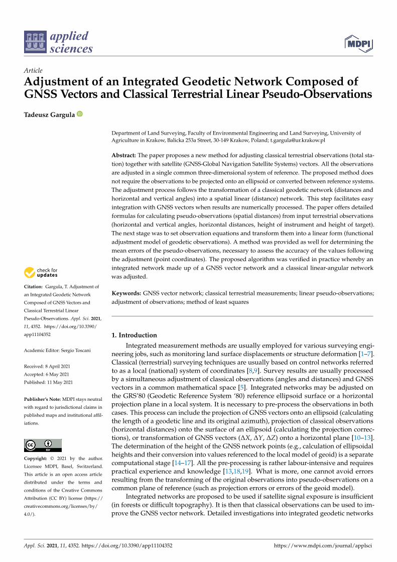
Figure 1. Normal distribution of measurement error (density function).

The error of measurement (ε) exhibits normal distribution if the error’s density func-tion f(ε) can be expressed as:

( )2 221 1 exp

22 2f e

ε εεπ π

− = ⋅ = ⋅ −

(1)

where: e—the base of a natural logarithm. The probability that the measurement error ε (as a random variable) will take a value

from the interval (ε1; ε2) can be expressed in the form (Figure 1):

( )2

1

2

1 21; exp

22P d

ε

ε

εε ε ε επ

−∈ = ⋅

(2)

where: dε—the differential of ε. As the actual values of errors of measurement ε are unknown, they are replaced with

observation corrections v, to be determined during adjustment. The goal of adjusting ob-servations with the least-squares method is to select such correction values v that the sum of their squares multiplied by the weights (p) is the smallest.

The principal idea behind the adjustment method proposed in this paper involves the transformation of a classical geodetic network (distances and horizontal and vertical angles) into a spatial linear (distance) network independent of the local reference system. The objective is to adjust a classical network and a GNSS vector network together in a common, geocentric XYZ coordinate system (referenced to the GRS’80 ellipsoid).

Figure 1. Normal distribution of measurement error (density function).

The error of measurement (ε) exhibits normal distribution if the error’s density func-tion f (ε) can be expressed as:

f (ε) =1√2π· e−

ε22 =

1√2π· exp

(− ε2

2

)(1)

where: e—the base of a natural logarithm.The probability that the measurement error ε (as a random variable) will take a value

from the interval (ε1; ε2) can be expressed in the form (Figure 1):

P(ε ∈ 〈ε1; ε2〉) =1√2π·

ε2∫ε1

exp(−ε2

2

)dε (2)

where: dε—the differential of ε.As the actual values of errors of measurement ε are unknown, they are replaced with

observation corrections v, to be determined during adjustment. The goal of adjustingobservations with the least-squares method is to select such correction values v that thesum of their squares multiplied by the weights (p) is the smallest.

The principal idea behind the adjustment method proposed in this paper involvesthe transformation of a classical geodetic network (distances and horizontal and verticalangles) into a spatial linear (distance) network independent of the local reference system.The objective is to adjust a classical network and a GNSS vector network together in acommon, geocentric XYZ coordinate system (referenced to the GRS’80 ellipsoid).

2. Materials and Methods2.1. Creating Linear Pseudo-Observations from the Classical Terrestrial Measurements

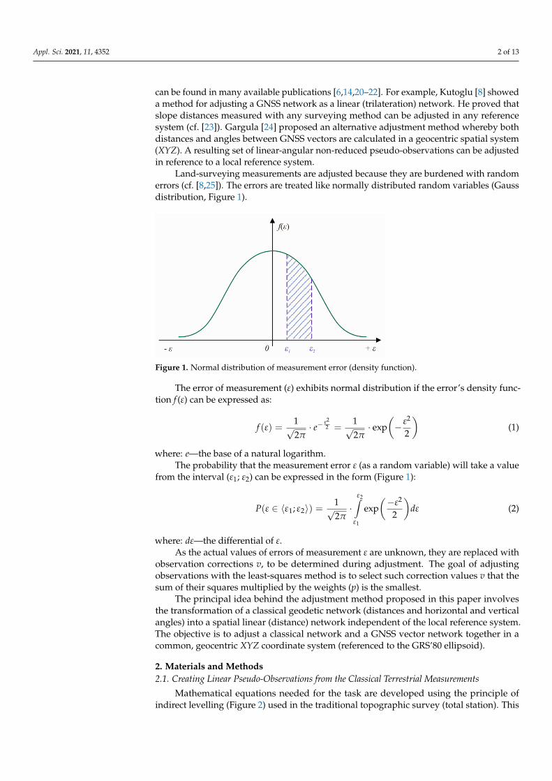
Mathematical equations needed for the task are developed using the principle ofindirect levelling (Figure 2) used in the traditional topographic survey (total station). This

Appl. Sci. 2021, 11, 4352 3 of 13

way one can calculate (using the Pythagorean theorem) the spatial (actual) distance betweentwo points of a geodetic network (j–instrument station, k–target position):

d2 = d2+ (i− s + h)2 (3)

Appl. Sci. 2021, 11, x FOR PEER REVIEW 3 of 14

2. Materials and Methods 2.1. Creating Linear Pseudo-Observations from the Classical Terrestrial Measurements

Mathematical equations needed for the task are developed using the principle of in-direct levelling (Figure 2) used in the traditional topographic survey (total station). This way one can calculate (using the Pythagorean theorem) the spatial (actual) distance be-tween two points of a geodetic network (j–instrument station, k–target position):

( )22 2= + − +d d i s h (3)

Figure 2. The principle of indirect levelling (O—tilt axis; C—target point; d—horizontal distance; d—spatial distance; i—height of instrument; s—height of signal/target; h—the difference in eleva-tion; α—vertical angle).

Next, the formulation to calculate the height difference h (see Figure 2) is substituted into Equation (3).

h=��× cotα (4)

This yields a general equation for the spatial distance between point j (station) and the measured point k as a function of the initial observations (d, α, i, s): 𝑑 = �� + 𝑖 − 𝑠 + 2 ⋅ 𝑖 − 𝑠 ⋅ �� ⋅ cot𝛼 + �� ⋅ cot 𝛼 (5)

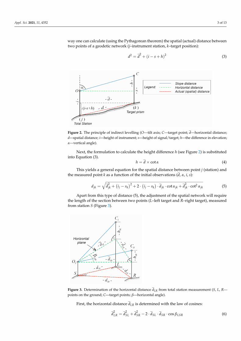
Apart from this type of distance (5), the adjustment of the spatial network will require the length of the section between two points (L–left target and R–right target), measured from station S (Figure 3).

Figure 3. Determination of the horizontal distance dLR from total station measurement (S, L, R—points on the ground; C—target points; β—horizontal angle).

Figure 2. The principle of indirect levelling (O—tilt axis; C—target point; d—horizontal distance;d—spatial distance; i—height of instrument; s—height of signal/target; h—the difference in elevation;α—vertical angle).

Next, the formulation to calculate the height difference h (see Figure 2) is substitutedinto Equation (3).

h = d× cot α (4)

This yields a general equation for the spatial distance between point j (station) andthe measured point k as a function of the initial observations (d, α, i, s):

djk =√

d2jk +

(ij − sk

)2+ 2 ·

(ij − sk

)· djk · cot αjk + d

2jk · cot2 αjk (5)

Apart from this type of distance (5), the adjustment of the spatial network will requirethe length of the section between two points (L–left target and R–right target), measuredfrom station S (Figure 3).

Appl. Sci. 2021, 11, x FOR PEER REVIEW 3 of 14

2. Materials and Methods 2.1. Creating Linear Pseudo-Observations from the Classical Terrestrial Measurements

Mathematical equations needed for the task are developed using the principle of in-direct levelling (Figure 2) used in the traditional topographic survey (total station). This way one can calculate (using the Pythagorean theorem) the spatial (actual) distance be-tween two points of a geodetic network (j–instrument station, k–target position):

( )22 2= + − +d d i s h (3)

Figure 2. The principle of indirect levelling (O—tilt axis; C—target point; d—horizontal distance; d—spatial distance; i—height of instrument; s—height of signal/target; h—the difference in eleva-tion; α—vertical angle).

Next, the formulation to calculate the height difference h (see Figure 2) is substituted into Equation (3).

h=��× cotα (4)

This yields a general equation for the spatial distance between point j (station) and the measured point k as a function of the initial observations (d, α, i, s): 𝑑 = �� + 𝑖 − 𝑠 + 2 ⋅ 𝑖 − 𝑠 ⋅ �� ⋅ cot𝛼 + �� ⋅ cot 𝛼 (5)

Apart from this type of distance (5), the adjustment of the spatial network will require the length of the section between two points (L–left target and R–right target), measured from station S (Figure 3).

Figure 3. Determination of the horizontal distance dLR from total station measurement (S, L, R—points on the ground; C—target points; β—horizontal angle).

Figure 3. Determination of the horizontal distance dLR from total station measurement (S, L, R—points on the ground; C—target points; β—horizontal angle).

First, the horizontal distance dLR is determined with the law of cosines:

d2LR = d

2SL + d

2SR − 2 · dSL · dSR · cos βLSR (6)

Appl. Sci. 2021, 11, 4352 4 of 13

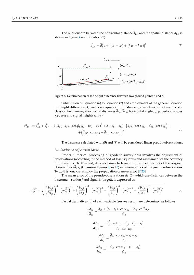
The relationship between the horizontal distance dLR and the spatial distance dLR isshown in Figure 4 and Equation (7).

d2LR = d

2LR + [(sL − sR) + (hSR − hSL)]

2 (7)

Appl. Sci. 2021, 11, x FOR PEER REVIEW 4 of 14

First, the horizontal distance dLR is determined with the law of cosines: 2 2 2 2 cos= + − ⋅ ⋅ ⋅LR SL SR SL SR LSRd d d d d β (6)

The relationship between the horizontal distance dLR and the spatial distance dLR is shown in Figure 4 and Equation (7).

Figure 4. Determination of the height difference between two ground points L and R.

( ) ( )[ ]22 2= + − + −LR LR L R SR SLd d s s h h (7)

Substitution of Equation (6) to Equation (7) and employment of the general Equation for height difference (4) yields an equation for distance dLR as a function of results of a classical field survey (horizontal distances dSL, dSR; horizontal angle βLSR; vertical angles αSL, αSR and signal heights sL, sR):

( ) ( ) ( )( )

22 2 2

2

2 cos 2 cot cot

cot cotLR SL SR SL SR LSR L R L R SR SR SL SL

SR SR SL SL

d d d d d s s s s d d

d d

β α αα α

= + − ⋅ ⋅ ⋅ + − + ⋅ − ⋅ ⋅ − ⋅ +

+ ⋅ − ⋅

(8)

The distances calculated with (5) and (8) will be considered linear pseudo-observa-tions.

2.2. Stochastic Adjustment Model Proper numerical processing of geodetic survey data involves the adjustment of ob-

servations (according to the method of least squares) and assessment of the accuracy of the results. To this end, it is necessary to transform the mean errors of the original obser-vations (d, α, β, I, s—see Figures 2 and 3) into mean errors of the pseudo-observations. To do this, one can employ the propagation of mean error [7,25].

The mean error of the pseudo-observations djk (5), which are distances between the instrument station j and signal k (target), is expressed as:

( ) ( )( ) ( )( ) ( )( ) ( )( )2 2 2 2

2 2 2 2 ∂ ∂ ∂ ∂ = ⋅ + ⋅ + ⋅ + ⋅ ∂ ∂ ∂ ∂

djk jk jk jkd i sjk jk jk j k

jk jk j k

d d d dm m m m m

d i sα

α (9)

Partial derivatives (∂) of each variable (survey result) are determined as follows:

( ) 2cot cot+ − ⋅ + ⋅∂=

∂jk j k jk jk jkjk

jk jk

d i s ddd d

α α

( )2

2

cotsin

− ⋅ − ⋅ −∂=

∂ ⋅jk jk jk j kjk

jk jk jk

d d i sdd

αα α

cot∂ ⋅ + −=

∂jk jk jk j k

j jk

d d i si d

α

Figure 4. Determination of the height difference between two ground points L and R.

Substitution of Equation (6) to Equation (7) and employment of the general Equationfor height difference (4) yields an equation for distance dLR as a function of results of aclassical field survey (horizontal distances dSL, dSR; horizontal angle βLSR; vertical anglesαSL, αSR and signal heights sL, sR):

d2LR = d

2SL + d

2SR − 2 · dSL · dSR · cos βLSR + (sL − sR)

2 + 2 · (sL − sR) ·(

dSR · cot αSR − dSL · cot αSL

)+

+(

dSR · cot αSR − dSL · cot αSL

)2 (8)

The distances calculated with (5) and (8) will be considered linear pseudo-observations.

2.2. Stochastic Adjustment Model

Proper numerical processing of geodetic survey data involves the adjustment ofobservations (according to the method of least squares) and assessment of the accuracyof the results. To this end, it is necessary to transform the mean errors of the originalobservations (d, α, β, I, s—see Figures 2 and 3) into mean errors of the pseudo-observations.To do this, one can employ the propagation of mean error [7,25].

The mean error of the pseudo-observations djk (5), which are distances between theinstrument station j and signal k (target), is expressed as:

m(d)jk =

√√√√(∂djk

∂djk

)2

·(

m(d)jk

)2+

(∂djk

∂αjk

)2

·(

m(α)jk

)2+

(∂djk

∂ij

)2

·(

m(i)j

)2+

(∂djk

∂sk

)2

·(

m(s)k

)2(9)

Partial derivatives (∂) of each variable (survey result) are determined as follows:

∂djk

∂djk=

djk +(ij − sk

)· cot αjk + djk · cot2 αjk

djk

∂djk

∂αjk=−d

2jk · cot αjk − djk ·

(ij − sk

)djk · sin2 αjk

∂djk

∂ij=

djk · cot αjk + ij − sk

djk

∂djk

∂sk=−djk · cot αjk −

(ij − sk

)djk

Appl. Sci. 2021, 11, 4352 5 of 13

The mean error of the pseudo-observations dLR (4), which are distances betweenthe left (L) and right (R) target (Figure 3), is determined as shown below (also using thepropagation of mean error):

m(d)LR =

√√√√√√(

∂dLR∂dSL

)2·(

m(d)SL

)2+(

∂dLR∂dSR

)2·(

m(d)SR

)2+(

∂dLR∂αSL

)2·(

m(α)SL

)2+(

∂dLR∂αSR

)2·(

m(α)SR

)2+

+(

∂dLR∂βLSR

)2·(

m(β)LSR

)2+(

∂dLR∂sL

)2·(

m(s)L

)2+(

∂dLR∂sR

)2·(

m(s)R

)2 (10)

Partial derivatives of each variable (survey results) are expressed with the follow-ing equations:

∂dLR∂dSL

=dSL−dSR ·cos βLSR−(sL−sR)·cot αSL−(dSR ·cot αSR−dSL ·cot αSL)·cot αSL

dLR;

∂dLR∂dSR

=dSR−dSL ·cos βLSR+(sL−sR)·cot αSR+(dSR ·cot αSR−dSL ·cot αSL)·cot αSR

dLR

∂dLR∂αSL

=(sL−sR)·dSL−(dSR ·cot αSR−dSL ·cot αSL)·dSL

sin2 αSL ·dLR;

∂dLR∂αSR

=−(sL−sR)·dSR−(dSR ·cot αSR−dSL ·cot αSL)·dSR

sin2 αSR ·dLR;

∂dLR∂βLSR

= dSL ·dSR ·sin βLSR ·cos βLSRdLR

;∂dLR∂sL

= sL−sR+dSR ·cot αSR−dSL ·cot αSLdLR

;∂dLR∂sR

= sR−sL+dSL ·cot αSL−dSR ·cot αSRdLR

.

The formulas for partial derivatives appearing in Equations (9) and (10) were verifiedalso for units.

The law of propagation of variance and covariance can be used to determine themean errors instead of the propagation of mean error (e.g., [8,25]) because consecutivepseudo-observations can depend on the same angles and distances. Nevertheless, basedon previous tests (cf. [24]), the actual effect of correlation of angles and distances on thevalues of calculated pseudo-observations is negligible.

The stochastic model for the integrated network is complemented with informationon a priori mean errors (m(∆x); m(∆y); m(∆z)) of components of the GNSS vector (∆xjk; ∆yjk;∆zjk), which can be obtained in post-processing [26].

2.3. Functional Adjustment Model

The creation of the functional model of the adjustment of a geodetic network involvesthe listing of observation equations and transforming them into linear equations of cor-rection. The formulas below are general equations for three types of observations (in anintegrated spatial geodetic network): (1) the station–target distance; (2) the left target–righttarget distance; (3) components of the GNSS vector.

(1) The station–target spatial distance (cf. Equation (5)):

djk + v(d)jk =√(

xk − xj)2

+(yk − yj

)2+(zk − zj

)2 (11)

v(d)jk =∂djk

∂xj· δxj +

∂djk

∂yj· δyj +

∂djk

∂zj· δzj +

∂djk

∂xk· δxk +

∂djk

∂yk· δyk +

∂djk

∂zk· δzk + l(d)jk (12)

l(d)jk = d(0)jk − djk (13)

where:

l(d)jk —the absolute term in the correction Equation (12);

d(0)jk =

√(x(0)k − x(0)j

)2+(

y(0)k − y(0)j

)2+(

z(0)k − z(0)j

)2—the approximate distance;

Appl. Sci. 2021, 11, 4352 6 of 13

∂djk∂xj

= −x(0)k −x(0)j

d(0)jk

;∂djk∂yj

= −y(0)k −y(0)j

d(0)jk

;∂djk∂zj

= −z(0)k −z(0)j

d(0)jk

∂djk∂xk

=x(0)k −x(0)j

d(0)jk

;∂djk∂yk

=y(0)k −y(0)j

d(0)jk

;∂djk∂zk

=z(0)k −z(0)j

d(0)jk

—partial derivatives;

x(0) y(0) z(0)—approximate coordinates.(2) The left target–right target spatial distance (cf. Equation (8)):

dLR + v(d)LR =

√(xR − xL)

2 + (yR − yL)2 + (zR − zL)

2 (14)

v(d)LR =∂dLR∂xL

· δxL +∂dLR∂yL

· δyL +∂dLR∂zL

· δzL +∂dLR∂xR

· δxR +∂dLR∂yR

· δyR +∂dLR∂zR

· δzR + l(d)LR (15)

l(d)LR = d(0)LR − dLR (16)

where:

l(d)LR —the absolute term in the correction Equation (15);

d(0)LR =

√(x(0)R − x(0)L

)2+(

y(0)R − y(0)L

)2+(

z(0)R − z(0)L

)2—the approximate distance.

The partial derivatives in Equation (15) are calculated similarly as for Equation (12).(3) The GNSS vector (∆x, ∆y, ∆z) between two points j and k:

∆xjk + v(∆x)jk = xk − xj

∆yjk + v(∆y)jk = yk − yj

∆zjk + v(∆z)jk = zk − zj

(17)

v(∆x)

jk =∂(∆x)jk

∂xk· δxk −

∂(∆x)jk∂xj

· δxj + l(∆x)jk = δxk − δxj + l(∆x)

jk

v(∆y)jk =

∂(∆y)jk∂yk

· δyk −∂(∆y)jk

∂xj· δyj + l(∆y)

jk = δyk − δyj + l(∆y)jk

v(∆z)jk =

∂(∆z)jk∂zk

· δzk −∂(∆z)jk

∂zj· δzj + l(∆z)

jk = δzk − δzj + l(∆z)jk

(18)

l(∆x)jk = ∆x(0)jk − ∆xjk

l(∆y)jk = ∆y(0)jk − ∆yjk

l(∆z)jk = ∆z(0)jk − ∆zjk

(19)

where:l(∆x), l(∆y), l(∆z)—absolute terms in the correction Equation (18);v(∆x), v(∆y), v(∆z)—corrections for the GNSS vector components;δx, δy, δz—the increments (corrections) to be determined for approximate coordinates;∆x(0), ∆y(0), ∆z(0)—approximate values of the GNSS vector calculated as:

∆x(0)jk = x(0)k − x(0)j

∆y(0)jk = y(0)k − y(0)j

∆z(0)jk = z(0)k − z(0)j

(20)

The partial derivatives in Equation (18) assume values 1 or –1 because the observationsin Equation (17) are linear (partial derivatives of linear equations calculated for unknownsare equal to the coefficients at these unknowns).

Appl. Sci. 2021, 11, 4352 7 of 13

2.4. The Procedure for Adjusting the Integrated Network

The adjustment of the integrated geodetic network (using the method of least squares)will be based on an overdetermined system of equations of correction type (12), (15) and(18), expressed as the following matrix form:

V = A · X− L (21)

where:

V =[{

v(d)jk ; v(d)LR ;(

v(∆x)jk ; v(∆y)

jk ; v(∆z)jk

)}]T—the vector of corrections type (12), (15) and (18)

to be determined (curly brackets { . . . } stand for all elements of a type);A—the matrix of coefficients of the unknowns (partial derivatives) in Equations (12), (15) and (18);

X =[{

(δxL; δyL; δzL; δxR; δyR; δzR);(δxj; δyj; δzj; δxk; δyk; δzk

)}]T—the vector of the un-knowns—increments to approximate coordinates;

L =[{

l(d)jk ; l(d)LR ;(

l(∆x)jk ; l(∆y)

jk ; l(∆z)jk

)}]T—the vector of absolute terms type (13), (16) and (19).

The estimated vector of the unknowns X is calculated with the method known fromthe adjustment calculus [13], which stems from the imposition of the least square condition(VT·P·V = min.) on the system (21):

X =(

AT · P ·A)−1

AT · P · L (22)

where:

P—the matrix of weights set up from mean errors of the linear pseudo-observations (9),(10) and mean errors of GNSS vector measurements (m(∆x); m(∆y); m(∆z)):

diag{P} =

1(m(d)

jk

)2 ;1(

m(d)LR

)2 ;

1(m(∆x)

jk

)2 ;1(

m(∆y)jk

)2 ;1(

m(∆z)jk

)2

(23)

The next step is to substitute the vector of unknowns X (21) with the calculated vectorX (22) and calculate the vector of observation corrections V, which are used to adjust theobservations—the left sides of the observation Equations (11), (14) and (17).

Information on mean errors of the adjusted coordinates (mx, my, mz) can be found onthe diagonal of the covariance matrix (Qx) of the vector X:

Qx = m0 ·(

AT · P ·A)−1

(24)

m0 =

√VT · P ·V

r(25)

where:

m0—the standard error of unit weight;r—the number of redundant observations.

Next, a single parameter characterising the point’s accuracy is calculated for eachpoint—the error of position (mP) in a three-dimensional Cartesian system:

mP =√

m2x + m2

y + m2z (26)

3. Results and Discussion (Numerical Example)

The proposed method for adjusting an integrated network was verified with a simplepractical example (Figure 5b). Calculations were performed for a GNSS vector network(without classical linear-angular observations, Figure 5a) as well, to compare the results.

Appl. Sci. 2021, 11, 4352 8 of 13

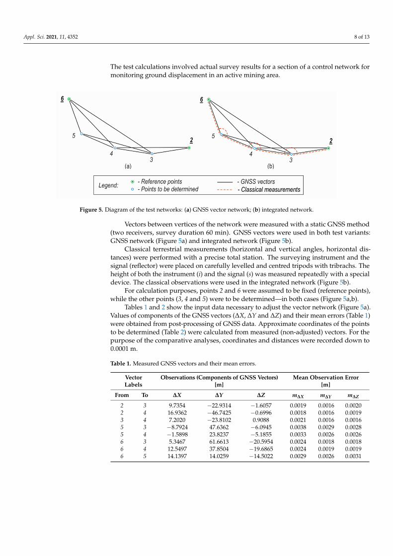
The test calculations involved actual survey results for a section of a control network formonitoring ground displacement in an active mining area.

Appl. Sci. 2021, 11, x FOR PEER REVIEW 9 of 14

Figure 5. Diagram of the test networks: (a) GNSS vector network; (b) integrated network.

Tables 1 and 2 show the input data necessary to adjust the vector network (Figure 5a). Values of components of the GNSS vectors (ΔX, ΔY and ΔZ) and their mean errors (Table 1) were obtained from post-processing of GNSS data. Approximate coordi-nates of the points to be determined (Table 2) were calculated from measured (non-ad-justed) vectors. For the purpose of the comparative analyses, coordinates and distances were recorded down to 0.0001 m.

Table 1. Measured GNSS vectors and their mean errors.

Vector Labels

Observations (Components of GNSS Vectors) [m]

Mean Observation Error [m]

From To ΔX ΔY ΔZ mΔX mΔY mΔZ

2 3 9.7354 −22.9314 −1.6057 0.0019 0.0016 0.0020

2 4 16.9362 −46.7425 −0.6996 0.0018 0.0016 0.0019

3 4 7.2020 −23.8102 0.9088 0.0021 0.0016 0.0016

5 3 −8.7924 47.6362 −6.0945 0.0038 0.0029 0.0028

5 4 −1.5898 23.8237 −5.1855 0.0033 0.0026 0.0026

6 3 5.3467 61.6613 −20.5954 0.0024 0.0018 0.0018

6 4 12.5497 37.8504 −19.6865 0.0024 0.0019 0.0019

6 5 14.1397 14.0259 −14.5022 0.0029 0.0026 0.0031

Table 2. Coordinates of reference points (2 and 6) and approximate coordinates (*) of points to be determined (3, 4, 5)—geocentric system ETRF’89.

Point X [m] Y [m] Z [m]

2 3,871,857.1432 1,345,974.9571 4,870,463.1848

3 * 3,871,866.8786 1,345,952.0257 4,870,461.5791

4 * 3,871,874.0806 1,345,928.2155 4,870,462.4879

5 * 3,871,875.6704 1,345,904.3918 4,870,467.6734

6 3,871,861.5368 1,345,890.3711 4,870,482.1739

Figure 5. Diagram of the test networks: (a) GNSS vector network; (b) integrated network.

Vectors between vertices of the network were measured with a static GNSS method(two receivers, survey duration 60 min). GNSS vectors were used in both test variants:GNSS network (Figure 5a) and integrated network (Figure 5b).

Classical terrestrial measurements (horizontal and vertical angles, horizontal dis-tances) were performed with a precise total station. The surveying instrument and thesignal (reflector) were placed on carefully levelled and centred tripods with tribrachs. Theheight of both the instrument (i) and the signal (s) was measured repeatedly with a specialdevice. The classical observations were used in the integrated network (Figure 5b).

For calculation purposes, points 2 and 6 were assumed to be fixed (reference points),while the other points (3, 4 and 5) were to be determined—in both cases (Figure 5a,b).

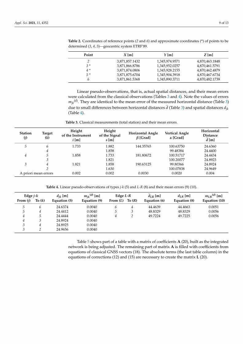
Tables 1 and 2 show the input data necessary to adjust the vector network (Figure 5a).Values of components of the GNSS vectors (∆X, ∆Y and ∆Z) and their mean errors (Table 1)were obtained from post-processing of GNSS data. Approximate coordinates of the pointsto be determined (Table 2) were calculated from measured (non-adjusted) vectors. For thepurpose of the comparative analyses, coordinates and distances were recorded down to0.0001 m.

Table 1. Measured GNSS vectors and their mean errors.

VectorLabels

Observations (Components of GNSS Vectors)[m]

Mean Observation Error[m]

From To ∆X ∆Y ∆Z m∆X m∆Y m∆Z

2 3 9.7354 −22.9314 −1.6057 0.0019 0.0016 0.00202 4 16.9362 −46.7425 −0.6996 0.0018 0.0016 0.00193 4 7.2020 −23.8102 0.9088 0.0021 0.0016 0.00165 3 −8.7924 47.6362 −6.0945 0.0038 0.0029 0.00285 4 −1.5898 23.8237 −5.1855 0.0033 0.0026 0.00266 3 5.3467 61.6613 −20.5954 0.0024 0.0018 0.00186 4 12.5497 37.8504 −19.6865 0.0024 0.0019 0.00196 5 14.1397 14.0259 −14.5022 0.0029 0.0026 0.0031

Appl. Sci. 2021, 11, 4352 9 of 13

Table 2. Coordinates of reference points (2 and 6) and approximate coordinates (*) of points to bedetermined (3, 4, 5)—geocentric system ETRF’89.

Point X [m] Y [m] Z [m]

2 3,871,857.1432 1,345,974.9571 4,870,463.18483 * 3,871,866.8786 1,345,952.0257 4,870,461.57914 * 3,871,874.0806 1,345,928.2155 4,870,462.48795 * 3,871,875.6704 1,345,904.3918 4,870,467.67346 3,871,861.5368 1,345,890.3711 4,870,482.1739

Linear pseudo-observations, that is, actual spatial distances, and their mean errorswere calculated from the classical observations (Tables 3 and 4). Note the values of errorsmjk

(d). They are identical to the mean error of the measured horizontal distance (Table 3)due to small differences between horizontal distances d (Table 3) and spatial distances djk(Table 4).

Table 3. Classical measurements (total station) and their mean errors.

Station(j)

Target(k)

Heightof the Instrument

i [m]

Heightof the Signal

s [m]

Horizontal Angleβ [Grad]

Vertical Angleα [Grad]

HorizontalDistance

d [m]

5 6 1.733 1.882 144.35765 100.63750 24.63604 1.858 99.48384 24.4400

4 5 1.858 1.733 181.80672 100.51717 24.44343 1.821 100.20077 24.8923

3 4 1.821 1.858 190.63125 99.80366 24.89242 1.630 100.07838 24.9649

A priori mean errors 0.002 0.002 0.0030 0.0020 0.004

Table 4. Linear pseudo-observations of types j-k (5) and L-R (8) and their mean errors (9) (10).

Edge j-k djk [m] mjk(d) [m] Edge L-R dLR [m] dLR [m] mLR

(d) [m]From (j) To (k) Equation (5) Equation (9) From (L) To (R) Equation (6) Equation (8) Equation (10)

5 6 24.6374 0.0040 6 4 44.4639 44.4663 0.00515 4 24.4412 0.0040 5 3 48.8329 48.8329 0.00564 5 24.4444 0.0040 4 2 49.7224 49.7225 0.00564 3 24.8924 0.00403 4 24.8925 0.00403 2 24.9656 0.0040

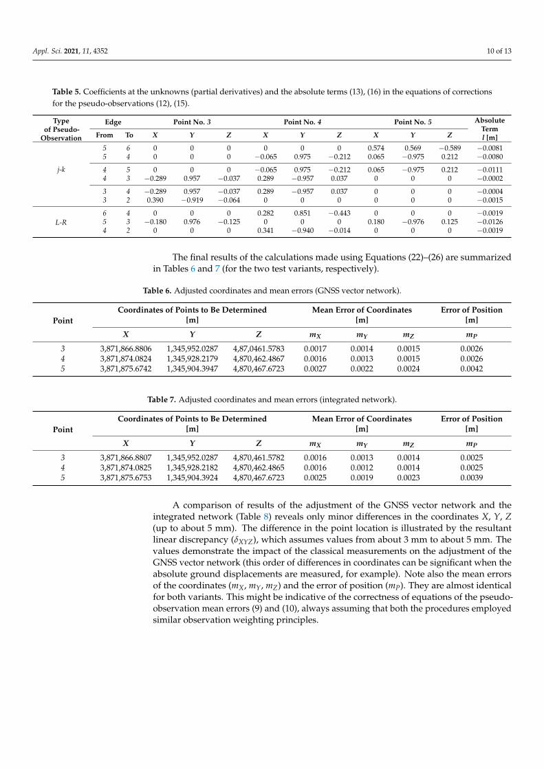
Table 5 shows part of a table with a matrix of coefficients A (20), built as the integratednetwork is being adjusted. The remaining part of matrix A is filled with coefficients fromequations of classical GNSS vectors (18). The absolute terms (the last table column) in theequations of corrections (12) and (15) are necessary to create the matrix L (20).

Appl. Sci. 2021, 11, 4352 10 of 13

Table 5. Coefficients at the unknowns (partial derivatives) and the absolute terms (13), (16) in the equations of correctionsfor the pseudo-observations (12), (15).

Typeof Pseudo-

Observation

Edge Point No. 3 Point No. 4 Point No. 5 AbsoluteTerml [m]From To X Y Z X Y Z X Y Z

j-k

5 6 0 0 0 0 0 0 0.574 0.569 −0.589 −0.00815 4 0 0 0 −0.065 0.975 −0.212 0.065 −0.975 0.212 −0.0080

4 5 0 0 0 −0.065 0.975 −0.212 0.065 −0.975 0.212 −0.01114 3 −0.289 0.957 −0.037 0.289 −0.957 0.037 0 0 0 −0.0002

3 4 −0.289 0.957 −0.037 0.289 −0.957 0.037 0 0 0 −0.00043 2 0.390 −0.919 −0.064 0 0 0 0 0 0 −0.0015

L-R6 4 0 0 0 0.282 0.851 −0.443 0 0 0 −0.00195 3 −0.180 0.976 −0.125 0 0 0 0.180 −0.976 0.125 −0.01264 2 0 0 0 0.341 −0.940 −0.014 0 0 0 −0.0019

The final results of the calculations made using Equations (22)–(26) are summarizedin Tables 6 and 7 (for the two test variants, respectively).

Table 6. Adjusted coordinates and mean errors (GNSS vector network).

PointCoordinates of Points to Be Determined

[m]Mean Error of Coordinates

[m]Error of Position

[m]

X Y Z mX mY mZ mP

3 3,871,866.8806 1,345,952.0287 4,87,0461.5783 0.0017 0.0014 0.0015 0.00264 3,871,874.0824 1,345,928.2179 4,870,462.4867 0.0016 0.0013 0.0015 0.00265 3,871,875.6742 1,345,904.3947 4,870,467.6723 0.0027 0.0022 0.0024 0.0042

Table 7. Adjusted coordinates and mean errors (integrated network).

PointCoordinates of Points to Be Determined

[m]Mean Error of Coordinates

[m]Error of Position

[m]

X Y Z mX mY mZ mP

3 3,871,866.8807 1,345,952.0287 4,870,461.5782 0.0016 0.0013 0.0014 0.00254 3,871,874.0825 1,345,928.2182 4,870,462.4865 0.0016 0.0012 0.0014 0.00255 3,871,875.6753 1,345,904.3924 4,870,467.6723 0.0025 0.0019 0.0023 0.0039

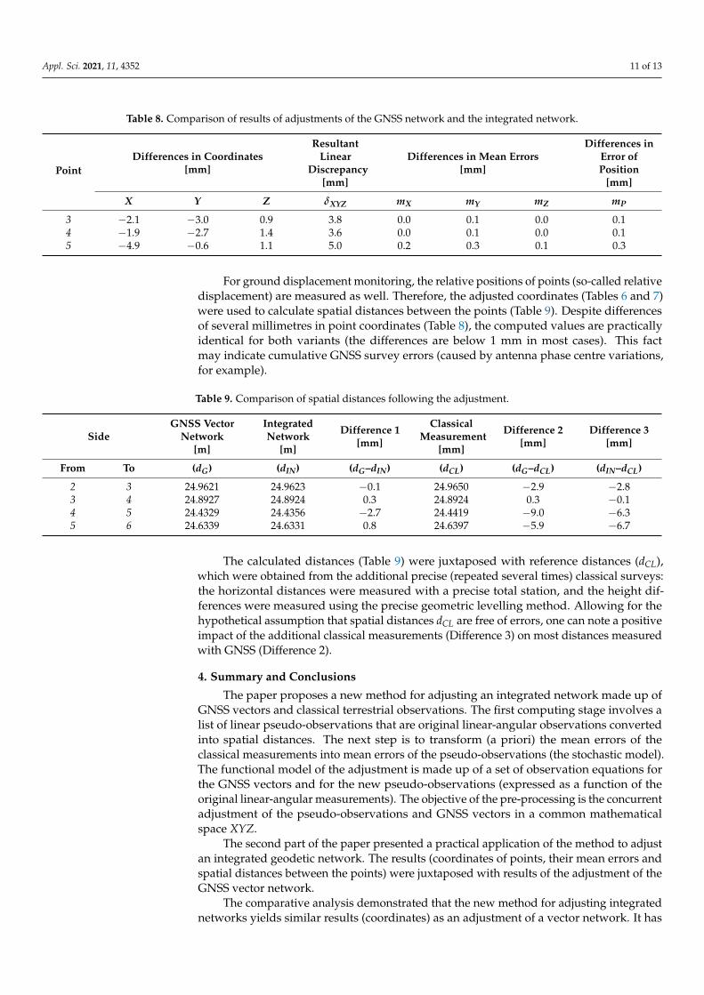
A comparison of results of the adjustment of the GNSS vector network and theintegrated network (Table 8) reveals only minor differences in the coordinates X, Y, Z(up to about 5 mm). The difference in the point location is illustrated by the resultantlinear discrepancy (δXYZ), which assumes values from about 3 mm to about 5 mm. Thevalues demonstrate the impact of the classical measurements on the adjustment of theGNSS vector network (this order of differences in coordinates can be significant when theabsolute ground displacements are measured, for example). Note also the mean errorsof the coordinates (mX, mY, mZ) and the error of position (mP). They are almost identicalfor both variants. This might be indicative of the correctness of equations of the pseudo-observation mean errors (9) and (10), always assuming that both the procedures employedsimilar observation weighting principles.

Appl. Sci. 2021, 11, 4352 11 of 13

Table 8. Comparison of results of adjustments of the GNSS network and the integrated network.

PointDifferences in Coordinates

[mm]

ResultantLinear

Discrepancy[mm]

Differences in Mean Errors[mm]

Differences inError ofPosition

[mm]

X Y Z δXYZ mX mY mZ mP

3 −2.1 −3.0 0.9 3.8 0.0 0.1 0.0 0.14 −1.9 −2.7 1.4 3.6 0.0 0.1 0.0 0.15 −4.9 −0.6 1.1 5.0 0.2 0.3 0.1 0.3

For ground displacement monitoring, the relative positions of points (so-called relativedisplacement) are measured as well. Therefore, the adjusted coordinates (Tables 6 and 7)were used to calculate spatial distances between the points (Table 9). Despite differencesof several millimetres in point coordinates (Table 8), the computed values are practicallyidentical for both variants (the differences are below 1 mm in most cases). This factmay indicate cumulative GNSS survey errors (caused by antenna phase centre variations,for example).

Table 9. Comparison of spatial distances following the adjustment.

SideGNSS Vector

Network[m]

IntegratedNetwork

[m]

Difference 1[mm]

ClassicalMeasurement

[mm]

Difference 2[mm]

Difference 3[mm]

From To (dG) (dIN) (dG–dIN) (dCL) (dG–dCL) (dIN–dCL)

2 3 24.9621 24.9623 −0.1 24.9650 −2.9 −2.83 4 24.8927 24.8924 0.3 24.8924 0.3 −0.14 5 24.4329 24.4356 −2.7 24.4419 −9.0 −6.35 6 24.6339 24.6331 0.8 24.6397 −5.9 −6.7

The calculated distances (Table 9) were juxtaposed with reference distances (dCL),which were obtained from the additional precise (repeated several times) classical surveys:the horizontal distances were measured with a precise total station, and the height dif-ferences were measured using the precise geometric levelling method. Allowing for thehypothetical assumption that spatial distances dCL are free of errors, one can note a positiveimpact of the additional classical measurements (Difference 3) on most distances measuredwith GNSS (Difference 2).

4. Summary and Conclusions

The paper proposes a new method for adjusting an integrated network made up ofGNSS vectors and classical terrestrial observations. The first computing stage involves alist of linear pseudo-observations that are original linear-angular observations convertedinto spatial distances. The next step is to transform (a priori) the mean errors of theclassical measurements into mean errors of the pseudo-observations (the stochastic model).The functional model of the adjustment is made up of a set of observation equations forthe GNSS vectors and for the new pseudo-observations (expressed as a function of theoriginal linear-angular measurements). The objective of the pre-processing is the concurrentadjustment of the pseudo-observations and GNSS vectors in a common mathematicalspace XYZ.

The second part of the paper presented a practical application of the method to adjustan integrated geodetic network. The results (coordinates of points, their mean errors andspatial distances between the points) were juxtaposed with results of the adjustment of theGNSS vector network.

The comparative analysis demonstrated that the new method for adjusting integratednetworks yields similar results (coordinates) as an adjustment of a vector network. It has

Appl. Sci. 2021, 11, 4352 12 of 13

further been demonstrated that an integrated network provides more accurate (close toreal) spatial distances between points (in relation to reference distances obtained fromprecise classical surveys).

The primary advantage of the proposed adjustment method is the ease of integrationof GNSS vectors with linear pseudo-observations obtained from classical measurements.The preparation of pseudo-observations is much easier than for other available methods foradjusting integrated networks (where it is necessary to determine the lengths of geodeticlines and their azimuths on the ellipsoid, project classical observations onto the ellipsoid,or convert ellipsoidal heights into orthometric values, etc.). The proposed method can beemployed to adjust periodic measurements of control networks for ground displacementmonitoring. However, the use of this calculation method is limited to short lines. Ifdistances between the points are longer than 200–300 m, the effect of refraction and thecurvature of the earth should be considered [27].

The research reported here will be continued. A detailed computing algorithm for themethod and its implementation as a computer application is planned. Furthermore, anattempt will be made to test the new adjustment method on a network with much longerGNSS vectors and pseudo-observations (about a few hundred metres).

Funding: This research received no external funding.

Institutional Review Board Statement: Not applicable.

Informed Consent Statement: Not applicable.

Data Availability Statement: The study did not report any data.

Conflicts of Interest: The authors declare no conflict of interest.

References1. Asteriadis, G.; Schwan, H. GPS and terrestrial measurements for detecting crustal movements in a seismic area. Surv. Rev. 1998,

34, 447–454. [CrossRef]2. Baryła, R.; Oszczak, S.; Koczot, B.; Szczechowski, B. A concept of using static GPS measurements for determination of vertical

and horizontal land deformations in the Main and Old City of Gdansk. Rep. Geod. 2007, 1/82, 17–24.3. Haberler-Weber, M. Analysis and interpretation of geodetic landslide monitoring data based on fuzzy systems. Nat. Hazards

Earth Syst. Sci. 2005, 5, 755–760. [CrossRef]4. Hekimoglu, S.; Erdogan, B.; Butterworth, S. Increasing the Efficacy of the Conventional Deformation Analysis Methods:

Alternative Strategy. J. Surv. Eng. 2010, 136, 53–62. [CrossRef]5. Kadaj, R. Models, Methods and Computing Algorithms of Kinematic Networks in Geodetic Measurements of Movements and Deformation of

Objects (Monograph in Polish); Publishing House of Agricultural University of Krakow: Krakow, Poland, 1998.6. Welsch, W.M. Problems of accuracies in combined terrestrial and satellite control networks. J. Geod. 1986, 60, 193–204. [CrossRef]7. Wisniewski, Z.; Kaminski, W. Estimation and Prediction of Vertical Deformations of Random Surfaces, Applying the Total Least

Squares Collocation Method. Sensors 2020, 20, 3913. [CrossRef] [PubMed]8. Ghilani, C.D. Adjustment Computations: Spatial Data Analysis; John Wiley & Sons. Inc.: Hoboken, NJ, USA, 2018.9. Kutoglu, H.S. Direct determination of local coordinates from GPS without transformation. Surv. Rev. 2009, 41, 162–173. [CrossRef]10. Gargula, T. The conception of integrated survey networks composed of modular networks and GPS vectors. Surv. Rev. 2009, 41,

301–313. [CrossRef]11. Gargula, T. A kinematic model of a modular network as applied for the determination of displacements. Geod. Cartogr. 2009, 58,

51–67.12. Kadaj, R. GPS vector networks with classical observations in terms of modernization of the national geodetic frameworks (in

Polish). In Proceedings of the 2nd Nationwide Scientific and Technical Conference on Numerical Cartography and ComputerScience in Geodesy, Rzeszów, Polanczyk, Solina, 27−29 September 2007; pp. 171–179.

13. Seeber, G. Satellite Geodesy; Walter de Gruyter: Berlin, Germany; New York, NY, USA, 2003. [CrossRef]14. Fotopoulos, G.; Kotsakis, C.; Sideris, M.G. How Accurately Can We Determine Orthometric Height Differences from GPS and

Geoid Data? J. Surv. Eng. 2003, 129, 1–10. [CrossRef]15. Krynski, J.; Łyszkowicz, A. Study on choice of global geopotential model for quasi-geoid determination in Poland. Geod. Cartogr.

2005, 54, 17–36.16. Osada, E.; Krynski, J.; Owczarek, M. Robust Method of Quasigeoid Modelling in Poland Based on GPS/Levelling Data with

Suport of Gravity Data. Geod. Cartogr. 2005, 54, 99–117.17. You, R.-J. Local Geoid Improvement Using GPS and Leveling Data: Case Study. J. Surv. Eng. 2006, 132, 101–107. [CrossRef]

Appl. Sci. 2021, 11, 4352 13 of 13

18. Leick, A. Two-dimensional geodetic models. In GPS Satellite Surveying; John Wiley & Sons. Inc.: Hoboken, NJ, USA, 2004;pp. 321–339.

19. Hlibowicki, R.; Krzywicka-Blum, E.; Galas, R.; Borkowski, A.; Osada, E.; Cacon, S. Advanced Geodesy and Geodetic Astronomy(Academic Book); PWN: Warszawa/Wrocław, Poland, 1988. (In Polish)

20. Gargula, T.; Kwinta, A.; Siejka, Z. The use of modular networks integrated with GPS measurements to determine the movements.Sci. Bull. Rzesz. Univ. Technol. Ser. Constr. Environ. Eng. 2012, 59, 95–107. (In Polish)

21. Kutoglu, H.S.; Ayan, T.; Mekik, Ç. Integrating GPS with national networks by collocation method. Appl. Math. Comput. 2006, 177,508–514. [CrossRef]

22. Zerbini, S.; Richter, B.; Rocca, F.; Van Dam, T.; Matonti, F. A Combination of Space and Terrestrial Geodetic Techniques to MonitorLand Subsidence: Case Study, the Southeastern Po Plain, Italy. J. Geophys. Res. Space Phys. 2007, 112, 1–12. [CrossRef]

23. Vanícek, P.; Steeves, R.R. Transformation of coordinates between two horizontal geodetic datums. J. Geod. 1996, 70, 740–745.[CrossRef]

24. Gargula, T. GPS Vector Network Adjustment in a Local System of Coordinates Based on Linear-Angular Spatial Pseudo-Observations. J. Surv. Eng. 2011, 137, 60–64. [CrossRef]

25. Wisniewski, Z. Adjustment Calculus in Geodesy (Academic Book); Publications of University of Warmia and Mazury in Olsztyn:Olsztyn, Poland, 2005. (In Polish)

26. Kudas, D.; Wnek, A. Validation of the number of tie vectors in post-processing using the method of frequency in a centric cube.Open Geosci. 2020, 12, 242–255. [CrossRef]

27. Schofield, W. Engineering Surveying; Elsevier Science & Technology Books: Oxford, UK, 2001.