Adaptive pointwise estimation for pure jump Lévy processes

ADAPTIVE KERNEL ESTIMATION OF THE LEVY DENSITY

MELINA BEC*, CLAIRE LACOUR**

April 5, 2011

Abstract. This paper is concerned with adaptive kernel estimation of the Levy densityn(x) for pure jump Levy processes. The sample path is observed at n discrete instantsin the ”high frequency” context (∆ = ∆n tends to zero while n∆n tends to ∞). Weconstruct a collection of kernel estimators of the function g(x) = xn(x) and proposetwo methods of local adaptive selection of the bandwidth. The quadratic pointwise riskof the adaptive estimators is studied in both cases. The rate of convergence is provedto be optimal up to a logarithmic factor. We give examples and simulation results forprocesses fitting in our framework.

Keywords. Adaptive Estimation; High frequency; Pure jump Levy process; Nonpara-metric Kernel Estimator.

1. Introduction

Consider (Lt, t ≥ 0) a real-valued Levy process with characteristic function given by:

(1) ψt(u) = E(exp iuLt) = exp (t

∫

R

(eiux − 1)N(dx)).

We assume that the Levy measure N(dx) admits a density n(x) and that the functiong(x) = xn(x) satisfies:

• (G1):∫

R|x|n(x)dx =

∫R|g(x)|dx <∞.

Under these assumptions, (Lt, t ≥ 0) is a pure-jump Levy process without drift and withfinite variation on compact sets. Moreover E(|Lt|) < ∞ (see Bertoin (1996)). Supposethat we have discrete observations (Lk∆, k = 1, ..., n) with sampling interval ∆. Our aimin this paper is the nonparametric adaptive kernel estimation of the function g(x) = xn(x)based on these observations under the asymptotic framework n tends to ∞. This subjecthas been recently investigated by several authors. Figueroa-Lopez and Houdre (2006) usea penalized projection method to estimate the Levy density on a compact set separatedfrom 0. Other authors develop an estimation procedure based on empirical estimations ofthe characteristic function ψ∆(u) of the increments (Z∆

k = Lk∆ − L(k−1)∆, k = 1, . . . , n)and its derivatives followed by a Fourier inversion to recover the Levy density. For low-frequency data (∆ is fixed), we can quote Watteel and Kulperger (2003), Jongbloed andvan der Meulen (2006), Neumann and Reiß (2009) and Comte and Genon-Catalot (2010).In the high frequency context, which is our concern in this paper, the problem is simplersince ψ∆(u) → 1 when ∆ → 0. This implies that ψ∆(u) need not to be estimated and cansimply be replaced by 1 in the estimation procedures. This is what is done in Comte and

* UMR CNRS 8145 MAP5, Universite Paris Descartes, ** Laboratoire de mathematiques, UniversiteParis-Sud 11.

1

hal-0

0583

221,

ver

sion

1 -

5 Ap

r 201

1

http://hal.archives-ouvertes.fr/hal-00583221/fr/

http://hal.archives-ouvertes.fr

2 MELINA BEC*, CLAIRE LACOUR**

Genon-Catalot (2009) and Comte and Genon-Catalot (2010). These authors start fromthe equality:

(2) E

[Z∆

k eiuZ∆

k

]= −iψ

′∆(u)

∆,

where g∗(u) =∫eiuxg(x)dx is the Fourier transform of g well defined under (G1).

Then, as ψ∆(u) ≃ 1, equation (2) writes E

[Z∆

k eiuZ∆

k

]≃ g∗(u) and gives an estimator

of g∗(u) as follows:

1

n∆

n∑

k=1

Z∆k e

iuZ∆k

Now, to recover g the authors apply Fourier inversion with cutoff parameter m. Here, werather introduce a kernel to make inversion possible:

1

n∆

n∑

k=1

Z∆k K

∗(uh)eiuZ∆k

which is in fact the Fourier transform of 1/(nh∆)∑n

k=1 Z∆k K((Z∆

k − x)/h). At the end,in the high frequency context, a direct method without Fourier inversion can be applied.Indeed, a consequence of (2) is that the empirical distribution:

µn(dz) =1

n∆

n∑

k=1

Z∆k δZ∆

k(dz)

weakly converges to g(z)dz. This suggests to consider kernel estimators of g of the form

(3) gh(x0) = Kh ⋆ µn(x) =1

n∆

n∑

k=1

Z∆k Kh(Z∆

k − x)

where Kh(x) = (1/h)K(x/h) and K(−x) = K(x) is a symetric kernel such that∫

|K(u)|du <∞ and

∫K(u)du = 1.

Below, we study the pointwise L2-risk of the estimators (gh(x)) and evaluate the rate of

convergence of this risk as n → ∞, ∆ = ∆n tends to 0 and h = hn tends to 0. Thisis done under Holder regularity assumptions for the function g. Note that a pointwisestudy involving a kernel estimator can be found in van Es et al. (2007) for more specificcompound Poisson processes.

In this paper, we study local adaptive bandwidth selection (which the previous authorsdo not consider). For a given value x0 ∈ R, we define two ways of selecting a bandwidth

h(x0) such that the resulting adaptive estimator gh(x0)(x0) automatically reaches the op-

timal rate of convergence corresponding to the unknown regularity of the function g. Inthe first method (Bandwidth Selection I) we define an estimator β(x0) of the unknownregularity β of g and plug in the estimated value in the optimal bandwidth hopt(β) thatis deduced from the L

2 risk study. The second method (Bandwidth Selection II) fol-lows the scheme developped by Goldenshluger and Lepski (2011) for density estimation.Introducing iterated kernel estimators:

gh,h′(x0) = Kh′ ⋆ gh(x0) = Kh ⋆ gh′(x0),

hal-0

0583

221,

ver

sion

1 -

5 Ap

r 201

1

ADAPTIVE KERNEL ESTIMATION OF THE LEVY DENSITY 3

a data-driven choice h(x0) is defined and the adaptive estimator is given by gh(x0)(x0).

In Section 2, we give notations and assumptions. In Section 3, we study the pointwisemean square error (MSE) of gh(x0) given in (3) for g belonging to a Holder class ofregularity. We present the two bandwidth selection methods in Section 4 and 5 togetherwith a risk bound for each adaptive estimator. The rate of convergence of the risk isoptimal up to a logarithmic loss which is expected in adaptive pointwise context. Examplesand simulations in our framework are discussed in Section 6 and some concluding remarksare given in Section 7. Proofs are gathered in Section 8.

2. Notations and assumptions

We present the assumptions on the kernel K and on the function g required to studythe estimation given by (3). First, we set some notations. We denote by u∗ the Fouriertransform of u, u∗(y) =

∫eiyxu(x)dx. and by ‖u‖, < u, v >, u ⋆ v the quantities

‖u‖2 =

∫|u(x)|2dx,

< u, v >=

∫u(x)v(x)dx with zz = |z|2 and u ⋆ v(x) =

∫u(y)v(x− y)dy.

Moreover, for any integrable and square-integrable functions u, u1, u2 such that u∗ ∈ L1,

we have:

(4) (u∗)∗(x) = 2πu(−x) and 〈u1, u2〉 = (2π)−1〈u∗1, u∗2〉.

2.1. Kernel Assumptions. Let K : R → R be integrable and such that

∀u,∫K(u)du = 1 and K(u) = K(−u).(5)

We recall that for l ≥ 1 an integer, K : R → R is a kernel of order l if functions u 7→ujK(u), j = 0, 1, ..., l are integrable and satisfy

∫ujK(u)du = 0,∀j ∈ {1, ..., l}.(6)

The kernels will have to satisfy some of the following assumptions.

• (Ker[1]) K is of order l = ⌊β⌋ and∫|x|β |K(x)|dx < +∞.

We define the parameter β later.• (Ker[2]) ‖K‖2 < +∞.• (Ker[3]) K∗ ∈ L

1.

Assumptions (Ker[i]), i = 1, 2, 3 are standard when working on problems of estimation bykernel methods.We note that there is a way to build a kernel of order l. Indeed, let u be a symmetricand integrable function such that u ∈ L

2,u∗ ∈ L1 and

∫u(y)dy = 1, and set for any given

integer l,

K(t) =l∑

k=1

(k

l

)(−1)k+1 1

ku

(t

k

)(7)

hal-0

0583

221,

ver

sion

1 -

5 Ap

r 201

1


The kernel K defined by (7) is a kernel of order l which satisfies assumptions (Ker[i])i = 1, 2, 3 (see Kerkyacharian et al. (2001) and Goldenshluger and Lepski (2011)).

2.2. Assumptions on g. The target function g has to satisfy the following assumptions.

• (G1) ‖g‖1 < +∞.• (G2) ‖g‖2 < +∞.

We introduce Holder classes.

Definition 2.1. (Holder class) Let β > 0, L > 0 and let l = ⌊β⌋ be the largest integerstrictly smaller than β. The Holder class H(β,L) on R is the set of all functions f : R −→R such that derivative f (l) exists and verifies:

|f (l)(x0) − f (l)(x′0)| ≤ L|x0 − x′0|β−l,∀x0, x′0 ∈ R.(8)

This allows us to introduce the following assumption

• (G3) g ∈ H(β,L).

(G3) is a classical regularity assumption in nonparametric estimation; it allows to quan-tify the bias (see Tsybakov (2009)).

• (G4) M := ‖g′‖∞ < +∞.• (G5) xg ∈ L

1 and P := 12π

∫|g∗′(u)|du < +∞.

3. Risk bound

In this section, the bandwidth h is fixed, thus we omit the subscript h for the sake ofsimplicity: we denote g = gh. Let x0 ∈ R. The usual bias variance decomposition of theMSE yields:

MSE(x0, h) := E[(g(x0) − g(x0))2] = E[(g(x0) − E[g(x0)])

2] + (E[g(x0)] − g(x0))2

But the bias needs further decomposition:

b(x0)2 := (E[g(x0)] − g(x0))

2 ≤ 2b1(x0)2 + 2b2(x0)

2

with the usual bias,

b1(x0) = Kh ⋆ g(x0) − g(x0),

and the bias resulting from the approximation of ψ∆(u) by 1,

b2(x0) = E[g(x0)] −Kh ⋆ g(x0).

We can provide the following bias bound:

Lemma 3.1. Under (Ker[1]), (G1), (G3) and (G4) we have:

b(x0)2 ≤ c1h

2β + c′1∆2.

with c1 = 2(L/l!

∫|K(v)||v|βdv

)2and c′1 = 2M2(‖g‖1‖K‖1)

2, where M is defined in(G4).

Moreover, the variance is controlled as follows:

hal-0

0583

221,

ver

sion

1 -

5 Ap

r 201

1


Lemma 3.2. Under (Ker[2]), (Ker[3]), (G1), (G2) and (G5), we have

V ar[g(x0)] ≤1

nh∆‖K‖2

2(P + ‖g‖22∆) ≤ c2

1

nh∆+ c′2

1

nh

with c2 = P‖K‖22 where P is defined in (G5), and c′2 = ‖g‖2

2‖K‖22.

Lemmas 3.1 et 3.2 lead us to the following risk bound:

Proposition 3.1. Under (Ker[1])-(Ker[3]) , (G1)-(G5) we have

MSE(x0, h) ≤ c1h2β + c2

1

nh∆+ c′2

1

nh+ c′1∆

2.(9)

Recall that ∆ = ∆n is such that limn→+∞ ∆n = 0, thus 1/nh is negligible compared to1/nh∆. For ∆2, we set the following condition:

∆3 ≤ 1

nh, nh→ +∞.(10)

We can then proceed to find the convergence rate, based on the first two terms. It is easily

seen that the optimal choice of h is hopt ∝ ((n∆)− 1

2β+1 ) and the associated rate has order

O((n∆)−

2β

2β+1

).

Proposition 3.2. Under the assumptions of Proposition 3.1 and under condition (10),

the choice hopt ∝ ((n∆)− 1

2β+1 ) minimizes the risk bound (9) and gives MSE(x0, hopt) =

O((n∆)−2β

2β+1 ).

We stress the fact that this result is new as previous works in estimation (adaptive ornot) do not deal with the pointwise risk.

4. Bandwidth selection I

As β is unknown, we need a data-driven selection of the bandwidth. Firstly, we use themethod introduced in Lepski (1991).

We set the following additional condition:

1

n<< ∆ <<

1

n1/3(11)

In other words, the asymptotic context is n∆ → +∞ and n∆3 → 0. It allows to ensurecondition (10) for all h. It follows from Proposition 3.2 that if h = hopt(β) then,

E[ghopt(β)(x0) − g(x0)]2 ≤ C(n∆)−

2β

2β+1 =: Cu2n,opt(β).(12)

We define

u2n(β) =

(n∆

log(n∆)

)− 2β

2β+1

and h(β) =

(n∆

log(n∆)

)− 12β+1

.

We set gβ = gh(β).In the following, we use the letter β for the true parameter. Moreover we assume that βbelongs to the set A = {α1, ..., αD} where α1 < ... < αD and D = ⌊(n∆)ξ⌋ with ξ a fixed

positive real. We choose β(x0) as follows:

β(x0) = max{α ∈ A, ∀α′ ∈ A/α′ ≤ α, |gα(x0) − gα′(x0)| ≤ cun(α′)

}

hal-0

0583

221,

ver

sion

1 -

5 Ap

r 201

1


with c ≥ c′ + 2N + 2B1, c′ = 8‖K‖2

√P + ‖g‖2

2

√2ξ + 4 and B1 = M‖g‖1‖K‖1, and

N :=L

l!

∫|K(v)||v|βdv and P :=

1

2π

∫|g∗′(v)|dv.(13)

Heuristically, β(x0) estimates the regularity index β.

Then, the estimator of interest is: gβ(x0)(x0). We can prove the following bound on the

quadratic risk of our adaptive estimator.

Theorem 4.1. Under the assumptions of Proposition 3.1 and if the |Zi|’s admit a momentof order z with z > 10 + 4ξ + (5 + 2ξ)/α1, we have, under condition (11),

E[|gβ(x0)(x0) − g(x0)|] ≤ cun(β).(14)

Theorem 4.1 states that our data driven estimator automatically reaches the optimalrate stated in Proposition 3.2, up to a logarithmic factor. Note that for pointwise adaptivedensity estimation, a logarithmic loss also occurs and has been proved to be neverthelessoptimal (see Butucea (2001)).

5. Bandwidth selection II

Now, we follow ideas given in Goldenshluger and Lepski (2010) for density estimation.We set:

V (h) = Clog(n∆)

nh∆with C = (c′/2) × ‖K‖2

2(P + ‖g‖22), c

′ ∈ R+,(15)

where P is defined in (13). Note that V (h) has the same order as the variance multipliedby log(n∆).

We define gh,h′(x0) = Kh′ ⋆ gh(x0) = Kh ⋆ gh′(x0). So we have

(16) gh,h′(x0) =1

n∆

n∑

k=1

Z∆k Kh′ ⋆ Kh(Z∆

k − x0).

Lastly we set

(17) A(h, x0) = suph′∈H

{|gh,h′(x0) − gh′(x0)|2 − V (h′)}+ with H = { jM , 1 ≤ j ≤M},

and M to be specified later.The adaptive bandwidth h is chosen as follows:

h(x0) = arg minh∈H

{A(h, x0) + V (h)}.

To simplify notations, we set h = h(x0).

Theorem 5.1. Let the assumptions of Proposition 3.1 hold and assume that there existsβ0 (known) such that β > β0. Choose M =

[(n∆)1/(2β0+1)

]in (17) and take c′ in (15)

such that c′ ≥ 96(1 ∨ ‖K‖∞). Then if the |Zi|’s admit a moment of order z such thatz ≥ 2(3 + 2/β0), we have

E[|g(x0) − gh(x0)|2] ≤ C

{infh∈H

{‖g − E[gh]‖2

∞ + V (h)}

+log(n∆)

n∆

}

hal-0

0583

221,

ver

sion

1 -

5 Ap

r 201

1


The comment following Theorem 4.1 also applies to the result of Theorem 5.1.

Let us discuss and compare the two methods. The advantages of Method I are the fol-lowing. Method I provides an estimator β(x0) of β. It is based directly on the differencesbetween the functions gh(α) which are easily calculated as empirical means while MethodII requires the evaluations of Kh ⋆ Kh′ , sometimes numerically costly.Nevertheless, the constants required to implement the two methods are not similar. InMethod I, N is difficult to estimate (because of L and β). It could be possible to compute arough estimator. In Method II, we are able to offer empirical natural quantities to replace‖g‖ or ‖g′‖∞. Hence, Method II does not require a constant depending on the regularityof the function.

We choose to implement the second method to illustrate our results on various examples.

6. Examples and Simulations

We give some illustrating examples.

Example 1. Compound Poisson processes. Let Lt =∑Nt

i=1 Yi, where (Nt) is a Poissonprocess with constant intensity c and (Yi) is a sequence of i.i.d random variables withdensity f independent of the process (Nt). Then, (Lt) is a Levy process with characteristicfunction

(18) ψt(u) = exp

(ct

∫

R

(eiux − 1)f(x)dx

).

Its Levy density is n(x) = cf(x) and thus g(x) = cxf(x).In the simulations below we have chosen for f the standard Gaussian density. Thus,

g(x) = cxf(x) = cxe−x2/2/√

2π and g∗(u) = ciue−u2/2. Assumptions (G1), (G2), (G4)and (G5) hold for g. Moreover g belongs to a Holder class of regularity β for all β > 0.Thus the rate is close to (n∆/ log(n∆))−1.

Example 2. The Levy-Gamma process. Let α > 0, γ > 0. The Levy-Gamma process(Lt) with parameters (γ, α) is such that, for all t > 0, Lt has Gamma distribution withparameters (γt, α), i.e the density:

αγt

Γ(γt)xγt−1e−αx

1x≥0.

The Levy density is n(x) = γx−1e−αx1x>0 so that g(x) = γe−αx

1x>0 satisfies assumptions(G1), (G2) and (G5). We have g∗(u) = γ/(α − iu).Although g does not satisfy (G3)-(G4), we have implemented the estimation method tostudy its robustness with regard to this assumption. Note that the simulations results aregood in this case also.

Example 3. The bilateral Levy-Gamma process (Kuchler and Tappe (2008)). Con-sider X,Y two independent random variables, X with distribution Γ(γ, α) and Y withdistribution Γ(γ′, α′).Then, Z = X −Y has bilateral gamma distribution with parameters

hal-0

0583

221,

ver

sion

1 -

5 Ap

r 201

1


(γ, α, γ′, α′), denoted by Γ(γ, α; γ′, α′). The characteristic function of Z is equal to:

(19) ψ(u) =

(α

α− iu

)γ ( α′

α′ + iu

)γ′

= exp (

∫

R

(eiux − 1)n(x)dx),

with

n(x) = x−1g(x),

and, for x ∈ R,

g(x) = γe−αx1(0,+∞)(x) − γ′e−α′|x|1(−∞,0)(x).

The bilateral Gamma process (Lt) has characteristic function ψt(u) = ψ(u)t. As theprevious example, (G1), (G2) and (G5) hold, and not (G3)-(G4). But simulations arequite satisfactory.

We have implemented the estimation method for processes listed in Examples 1-3 withdifferent kernels (Figure 1) :

1. Epanechnikov Kernel: K(x) = (3/4)(1 − x2)1|x|≤1.2. Laplace Kernel: K(x) = (θ/2) exp(−|x|/θ) with θ = 1.3. Kernel K in Section 2 (see (7)) with l = 2 and l = 3. We choose u(x) =

1/√

2π exp (−x2/2), the Gaussian density.

The first two kernels are of order 1. Kernel [3.] is of order l = 2 or l = 3. For theimplementation, a difficulty is the proper calibration of the constant c′ in (15). This isusually done by a large number of previous simulations. We have chosen c′ = 1 as theadequate value for a variety of models, kernels and number of observations. As expected,when n∆ increases, the estimation is better. For clarity, we have computed the MeanIntegrated Square Error (MISE) of the estimators whose value gets smaller as n∆ increases.Figure 1 plots ten estimated curves corresponding to our three examples with in the firstcolumn n = 10000, ∆ = 0.1, and in the second n = 100000, ∆ = 0.1. Globally, it canbe seen from Figure 1 that the results are stable even for smaller values of n∆. Forillustration, each example presented in Figure 1 is computed with a specific kernel. Wedid not observe significant improvement when using the higher order kernel ([3.]). Thisis surprising because the theoretical part suggests that it should improve the bias term.Lastly, we can see that the estimated curves are not very regular when n∆ is not largeenough, this is due to the pointwise bandwidth selection.

7. Concluding remarks

In this paper, we have investigated in the high frequency framework the nonparametricestimation of the Levy density n(.) of pure jump Levy process. This is done through theestimation of the function g(x) = xn(x), and we use kernel estimators. We have studiedtwo methods of bandwidth selection. The rate we obtained are not the optimal ones, butthe logarithmic loss which occurs is negligible. Implementation of Method II on simulateddata illustrates the quality of the estimation even when some assumptions are not fulfilled.

8. Proofs

For many proofs, we need the two following Propositions (see Proposition 2.1 in Comteand Genon-Catalot (2010) and Proposition 2.1 in Comte and Genon-Catalot (2009)).

hal-0

0583

221,

ver

sion

1 -

5 Ap

r 201

1


Ex 1 (n∆ = 1000) MISE= 7, 9.10−3 Ex 1 (n∆ = 10000) MISE= 4, 6.10−3

−4 −3 −2 −1 0 1 2 3 4−0.4

−0.3

−0.2

−0.1

0

0.1

0.2

0.3MISE=0.0079673

−4 −3 −2 −1 0 1 2 3 4−0.4

−0.3

−0.2

−0.1

0

0.1

0.2

0.3MISE=0.0046332

Ex 2 (n∆ = 1000) MISE= 6, 5.10−2 Ex 2 (n∆ = 10000) MISE= 6, 1.10−2

0 1 2 3 4 5 6 7 80

0.1

0.2

0.3

0.4

0.5

0.6

0.7

0.8

0.9

1MISE=0.065101

0 1 2 3 4 5 6 7 80

0.1

0.2

0.3

0.4

0.5

0.6

0.7

0.8

0.9

1MISE=0.061793

Ex 3 (n∆ = 1000) MISE=0, 24 Ex 3 (n∆ = 10000) MISE=0, 17

−8 −6 −4 −2 0 2 4 6 8−1

−0.8

−0.6

−0.4

−0.2

0

0.2

0.4

0.6

0.8

1MISE=0.2428

−8 −6 −4 −2 0 2 4 6 8−1

−0.8

−0.6

−0.4

−0.2

0

0.2

0.4

0.6

0.8

1MISE=0.17151

Figure 1. Adaptive estimators of g. First line: Example 1 (CompoundPoisson and Gaussian density) with c = 1, using the Epanechnikov kernel.Second line: Example 2 (Levy Gamma) with α = γ = 1 using the Laplacekernel. Third line: Example 3 (Bilateral Levy Gamma) with α = γ = α′ =γ′ = 1 using kernel [3.].

hal-0

0583

221,

ver

sion

1 -

5 Ap

r 201

1


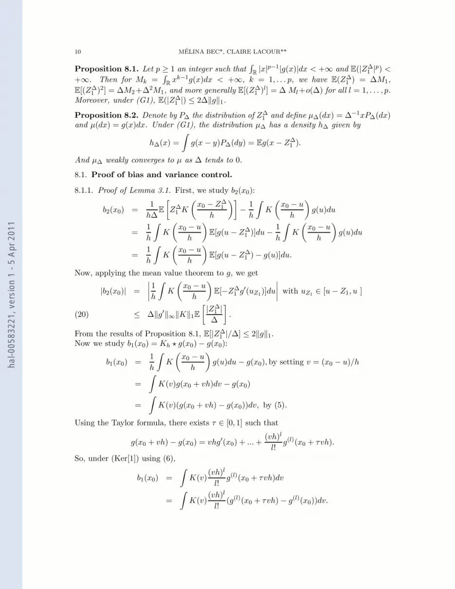
Proposition 8.1. Let p ≥ 1 an integer such that∫

R|x|p−1|g(x)|dx < +∞ and E(|Z∆

1 |p) <+∞. Then for Mk =

∫Rxk−1g(x)dx < +∞, k = 1, . . . p, we have E(Z∆

1 ) = ∆M1,

E[(Z∆1 )2] = ∆M2+∆2M1, and more generally E[(Z∆

1 )l] = ∆ Ml+o(∆) for all l = 1, . . . , p.Moreover, under (G1), E(|Z∆

1 |) ≤ 2∆‖g‖1.

Proposition 8.2. Denote by P∆ the distribution of Z∆1 and define µ∆(dx) = ∆−1xP∆(dx)

and µ(dx) = g(x)dx. Under (G1), the distribution µ∆ has a density h∆ given by

h∆(x) =

∫g(x− y)P∆(dy) = Eg(x− Z∆

1 ).

And µ∆ weakly converges to µ as ∆ tends to 0.

8.1. Proof of bias and variance control.

8.1.1. Proof of Lemma 3.1. First, we study b2(x0):

b2(x0) =1

h∆E

[Z∆

1 K

(x0 − Z∆

1

h

)]− 1

h

∫K

(x0 − u

h

)g(u)du

=1

h

∫K

(x0 − u

h

)E[g(u− Z∆

1 )]du− 1

h

∫K

(x0 − u

h

)g(u)du

=1

h

∫K

(x0 − u

h

)E[g(u− Z∆

1 ) − g(u)]du.

Now, applying the mean value theorem to g, we get

|b2(x0)| =

∣∣∣∣1

h

∫K

(x0 − u

h

)E[−Z∆

1 g′(uZ1)]du

∣∣∣∣ with uZ1 ∈ [u− Z1, u ]

≤ ∆‖g′‖∞‖K‖1E

[ |Z∆1 |

∆

].(20)

From the results of Proposition 8.1, E[|Z∆1 |/∆] ≤ 2‖g‖1.

Now we study b1(x0) = Kh ⋆ g(x0) − g(x0):

b1(x0) =1

h

∫K

(x0 − u

h

)g(u)du − g(x0),by setting v = (x0 − u)/h

=

∫K(v)g(x0 + vh)dv − g(x0)

=

∫K(v)(g(x0 + vh) − g(x0))dv, by (5).

Using the Taylor formula, there exists τ ∈ [0, 1] such that

g(x0 + vh) − g(x0) = vhg′(x0) + ...+(vh)l

l!g(l)(x0 + τvh).

So, under (Ker[1]) using (6),

b1(x0) =

∫K(v)

(vh)l

l!g(l)(x0 + τvh)dv

=

∫K(v)

(vh)l

l!(g(l)(x0 + τvh) − g(l)(x0))dv.

hal-0

0583

221,

ver

sion

1 -

5 Ap

r 201

1


It follows that

|b1(x0)| ≤∫

|K(v)| |vh|l

l!|g(l)(x0 + τvh) − g(l)(x0)|dv

≤∫

|K(v)| |vh|l

L|τvh|β−ldv,using (8) in (G3)

≤ hβL

l!

∫|K(v)||v|βdv :=

√c1/2h

β,(21)

as τ ∈ [0, 1] and∫|K(v)||v|βdv < +∞ under (Ker[1]).

Gathering (20) and (21), we obtain

b(x0)2 ≤ 2b1(x0)

2 + 2b2(x0)2

≤ c1h2β + 2M2(∆‖g‖1‖K‖1)

2.

This completes the proof of Lemma 3.1. 2

8.1.2. Proof of Lemma 3.2. We have the following relation:

ψ∆′′ = i∆ψ∆

′g∗ + i∆ψ∆g∗′ = −∆2ψ∆g

∗2 + i∆ψ∆g∗′.(22)

As the Z∆k are i.i.d., we have:

V ar[g(x0)] = V ar

[1

nh∆

n∑

k=1

Z∆k K

(Z∆

k − x0

h

)]

=1

n(h∆)2V ar

[Z∆

1 K

(Z∆

1 − x0

h

)].

Thus,

V ar[g(x0)] ≤1

n(h∆)2E

[(Z∆

1 )2K2

(Z∆

1 − x0

h

)].

Writing

K2

(Z∆

1 − x0

h

)=

∣∣∣∣1

2π

∫K∗(u)e−i

(x0−Z∆1 )u

h du

∣∣∣∣2

,

we obtain with v = u/h

V ar[g(x0)] ≤ 1

n∆2E

[

(Z∆1 )2

∣∣∣∣1

2π

∫K∗(vh)e−i(x0−Z∆

1 )vdv

∣∣∣∣2]

≤ 1

n∆2(2π)2E

[∫ ∫Z∆

1 eiZ∆

1 vK∗(vh)e−ix0vZ∆1 e

iZ∆1 uK∗(uh)e−ix0udvdu

].

Using Fubini (under (Ker[3])), E[(Z∆1 )2eiZ

∆1 (v−u)] = −ψ′′

∆(v−u) and formula (22), we find

V ar[g(x0)] ≤ 1

n∆2(2π)2

∫ ∫| − ψ∆

′′(v − u)K∗(vh)K∗(uh)|dvdu

≤ 1

n∆2(2π)2

∫ ∫|∆2ψ∆(v − u)(g∗)2(v − u)K∗(vh)K∗(uh)|dvdu

+1

n∆2(2π)2

∫ ∫|∆ψ∆(v − u)(g∗)′(v − u)K∗(vh)K∗(uh)|dvdu,with (22)

≤ T1 + T2

hal-0

0583

221,

ver

sion

1 -

5 Ap

r 201

1


with

T1 =1

n∆2(2π)2

∫ ∫|∆2ψ∆(v − u)(g∗)2(v − u)K∗(vh)K∗(uh)|dvdu

T2 =1

n∆2(2π)2

∫ ∫|∆ψ∆(v − u)(g∗)′(v − u)K∗(vh)K∗(uh)|dvdu.

We first bound T2:

T2 ≤ 1

n∆(2π)2

√∫ ∫|ψ∆(v − u)||(g∗)′(v − u)||K∗(vh)|2dvdu

×√∫ ∫

|ψ∆(v − u)||(g∗)′(v − u)||K∗(uh)|2dvdu

≤ 1

n∆(2π)2

∫|K∗(vh)|2dv

∫|ψ∆(z)||(g∗)′(z)|dz

≤ 1

nh∆(2π)2

∫|K∗(u)|2du

∫|(g∗)′(z)|dz, setting u = vh and because |ψ∆(z)| ≤ 1

≤ ‖K‖22

2πnh∆

∫|(g∗)′(z)|dz,where ‖K‖2 < +∞ by (Ker[2])

=P‖K‖2

2

nh∆, by (G5).

Following the same line for the study of T1, we get

T1 ≤ ‖K‖22

(2π)nh

∫|(g∗)2(z)|dz ≤ ‖K‖2

2‖g‖22

nh,

where ‖K‖2 < +∞ by (Ker[2]) and where ‖g‖2 < +∞ by (G2). This completes the proofof Lemma 3.2. 2

8.2. Proof of Theorem 4.1. We decompose E[|gβ(x0)(x0) − g(x0)|] as follows:

E[|gβ(x0)(x0) − g(x0)|] = E

[|gβ(x0)(x0) − g(x0)|1{β(x0)≥β}

](23)

+ E

[|gβ(x0)(x0) − g(x0)|1{β(x0)<β}

].

We bound the first term by simply using the definition of β(x0). We obtain

|gβ(x0) − gβ(x0)(x0)|1{β(x0)≥β} ≤ cun(β).

Also,

E

[|g(x0) − gβ(x0)(x0)|1{β(x0)≥β}

]≤ E|g(x0) − gβ(x0)| + E

[|gβ(x0) − gβ(x0)(x0)|1{β(x0)≥β}

]

≤ cun(β)(24)

hal-0

0583

221,

ver

sion

1 -

5 Ap

r 201

1


which completes the bound of the first term of (23).We now study the second term. We write

E[|gβ(x0)(x0) − g(x0)|1{β(x0)<β}] ≤(

E[|gβ(x0)(x0) − g(x0)|2])1/2

× P(β(x0) < β)1/2

≤(

E[|gβ(x0)(x0)|2] + ‖g‖2∞)1/2

× P(β(x0) < β)1/2

(25)

Proposition 8.3. Under the assumptions of Proposition 3.1 and if the |Zi|’s admit amoment of order z with z > 10+4ξ+(5+2ξ)/α1, under condition (11), there exists κ > 0such that

P(β(x0) < β) ≤ (2 + κ)(n∆)−4.

Proposition 8.4. Under (G1) and (G5), we have

E[|gβ(x0)(x0)|2] ≤ Q(n∆)2

log(n∆)2,

with Q := ‖K‖2∞(E[(Z∆

1 )2/∆] +[E[|Z∆

1 |/∆]]2)

.

Propositions 8.3, 8.4 and equation (25) imply that

E[|gβ(x0)(x0) − g(x0)|1{β(x0)<β}] ≤(Q(n∆)2 + ‖g‖2

∞)1/2√

(2 + κ)(n∆)−4 ≤ Q1

n∆(26)

where Q1 is a constant which depends on the terms E[Z∆1

2/∆] +

[E[Z∆

1 /∆]]2

and ‖g‖∞.We conclude by gathering (24) and (26):

E[|gβ(x0)(x0) − g(x0)|] = E[|gβ(x0)

(x0) − g(x0)|1{β(x0)≥β}] + E[|gβ(x0)(x0) − g(x0)|1{β(x0)≤β}]

≤ cun(β) +Q1(n∆)−1

≤ Cun(β).

This completes the proof of Theorem 4.1. 2

8.2.1. Proof of Proposition 8.3. We recall that gα(x0) = gh(α)(x0). First we write that

P(β(x0) < β) =∑

αi∈A,αi<β

P(β(x0) = αi)

=∑

αi∈A,αi<β

P(∃α′ ≤ αi+1|gαi+1(x0) − gα′(x0)| > cun(α′))

≤∑

αi+1≤β

∑

α′≤αi+1

P(|gαi+1(x0) − gα′(x0)| > cun(α′))

≤ D2 supα′≤α≤β

P(|gα(x0) − gα′(x0)| > cun(α′)).(27)

hal-0

0583

221,

ver

sion

1 -

5 Ap

r 201

1


Now we study P(|gα(x0) − gα′(x0)| > cun(α′)) for α′ ≤ α ≤ β. We have, with Lemma 3.1

|gα(x0) − gα′(x0)| ≤ |gα(x0) − gα(x0)| + |gα(x0) − g(x0)| + |g(x0) − gα′(x0)|+|gα′(x0) − gα′(x0)|(28)

≤ |gα(x0) − gα(x0)| + |gα′(x0) − gα′(x0)| +c12h(α)β +

c12h(α′)β + c′1∆

≤ |gα(x0) − gα(x0)| + |gα′(x0) − gα′(x0)|

+c12

(n∆

log(n∆))

−β

2α+1 +c12

(n∆

log(n∆))

−β

2α′+1 + c′1∆

≤ |gα(x0) − gα(x0)| + |gα′(x0) − gα′(x0)| + (c1 + c′1)un(α′),(29)

where (29) follows by using condition (11). Indeed for α′ ≤ α ≤ β, we have

(n∆

log(n∆)

) −β

2α+1

+

(n∆

log(n∆)

) −β

2α′+1

≤ 2

(n∆

log(n∆)

) −α′

2α′+1

= 2un(α′).

Therefore, we get

P(|gα(x0) − gα′(x0)| > cun(α′)) ≤ P(|gα(x0) − gα(x0)| + |gα′(x0) − gα′(x0)| > c′un(α′)),

with c′ = c− c1 − c′1.Now,

P(|gα(x0) − gα(x0)| + |gα′(x0) − gα′(x0)| > c′un(α′)) ≤ P(|gα(x0) − gα(x0)| > (c′/2)un(α′))

+ P(|gα′(x0) − gα′(x0)| > (c′/2)un(α′)),

and since, un(α′) ≥ un(α) we have

P(|gα(x0) − gα(x0)| > (c′/2)un(α′)) ≤ P(|gα(x0) − gα(x0)| > (c′/2)un(α)).(30)

Thus, we just have to bound 2P(|gα(x0) − gα(x0)| > (c′/2)un(α)) for all α ≤ β.Note that

gα(x0) − gα(x0) =1

n

n∑

k=1

[Yk(α) − E(Yk(α))](31)

where

Yk(α) =Zk

∆

∆h(α)K

(Zk

∆ − x0

h(α)

).(32)

We truncate the Zk∆ and we consider the decomposition:

{|Zk∆| ≤ µn}, and {|Zk

∆| > µn}

where

(33) µn = k(n∆

log(n∆))

α2α+1 with k =

‖K‖22(P + ‖g‖2

2)

c′‖K‖∞.

hal-0

0583

221,

ver

sion

1 -

5 Ap

r 201

1


We decompose (31),

gα(x0) − gα(x0) =1

n

n∑

k=1

[Yk(α)1{|Zk∆|≤µn} − E(Yk(α)1{|Zk

∆|≤µn})]

+1

n

n∑

k=1

[Yk(α)1{|Zk∆|>µn} − E(Yk(α)1{|Zk

∆|>µn})]

:= (g(1)α (x0) − gα

(1)(x0)) + (g(2)α (x0) − gα

(2)(x0)).

So we write

P(|gα(x0) − gα(x0)| > (c′/2)un(α))

≤ P(|g(1)α (x0) − gα

(1)(x0)| + |g(2)α (x0) − gα

(2)(x0)| > (c′/2)un(α))

≤ P(|g(1)α (x0) − gα

(1)(x0)| > c′un(α)/4) + P(|g(2)α (x0) − gα

(2)(x0)| > c′un(α)/4).(34)

We need the two following lemmas to conclude the proof.

Lemma 8.1. Under (Ker[2]) (Ker[3]) , (G1) (G2) et (G5) we have,

P(|g(1)α (x0) − gα

(1)(x0)| > c′un(α)/4) ≤ 2(n∆)−(2ξ+4).

Lemma 8.2. If the |Zi| admits a moment of order z with z > 10 + 4ξ + (5 + 2ξ)/α thereexists κ > 0 such that

P(|g(2)α (x0) − gα

(2)(x0)| > c′un(α)/4) ≤ κ(n∆)−(2ξ+4).

Thus we bound (34) by using Lemmas 8.1 and 8.2 and by gathering this with (27) and(30), we obtain:

P(β(x0) < β) ≤ D2 supα≤β

P(|gα(x0) − gα(x0)| > (c′/2)un(α))

≤ D2 supα≤β

P(|g(1)α (x0) − gα

(1)(x0)| > c′un(α)/4)

+ D2 supα≤β

P(|g(2)α (x0) − gα

(2)(x0)| > c′un(α)/4)

≤ 2(n∆)−4 + κ(n∆)−4.

This completes the proof of Proposition 8.3. 2

8.2.2. Proof of Proposition 8.4.

E[|gβ(x0)(x0)|2] ≤ E

{

1

nh(β(x0))∆

n∑

k=1

Z∆k K

(Z∆

k − x0

h(β(x0))

)}2

≤ ‖K‖2∞

(n∆)2E

1

h(β(x0))2

{n∑

k=1

|Z∆k |}2

.

We have, as β(x0) > 0 and thus 22β(x0)+1

< 2,

1

h(β(x0))2=

(n∆

log(n∆)

) 2

2β(x0)+1

<

(n∆

log(n∆)

)2

.

hal-0

0583

221,

ver

sion

1 -

5 Ap

r 201

1


We can write

E[|gβ(x0)(x0)|2] ≤ ‖K‖2∞

(n∆)2(n∆)2

log(n∆)2E

{

n∑

k=1

|Z∆k |}2

≤ ∆‖K‖2∞

log(n∆)2E

1

∆

{n∑

k=1

|Z∆k |}2

.(35)

Yet,

E

{

n∑

k=1

|Z∆k |}2

= V ar

[n∑

k=1

|Z∆k |]

+ E

[n∑

k=1

|Z∆k |]2

= nV ar[|Z∆

1 |]+[nE[|Z∆

1 |]]2

≤ n∆E[(Z∆1 )2/∆] + (n∆)2

[E[|Z∆

1 |/∆]]2

≤ (n∆)2(E[(Z∆

1 )2/∆] +[E[|Z∆

1 |/∆]]2)

.(36)

Therefore, inserting (35) in (36) completes the proof of Proposition 8.4. 2

8.2.3. Proof of lemmas 8.1 and 8.2. :

Proof of lemma 8.1 :We apply the Bernstein inequality recalled in Section 9 to Ti = Yi(α)1|Z∆

i |≤µnwhere

Yi(α) is defined by (32) and µn is defined by (33) (see Birge and Massart (1998), p.366).We choose η = c′un(α)/4. It is easy to see that

|Ti| ≤ b :=‖K‖∞µn

∆h(α)and V ar(Ti) ≤ ν2 := (P + ‖g‖2

2)‖K‖2

2

∆h(α).

We find

exp

(−nη2

4ν2

)= exp

(−nη4b

)= (n∆)−k1 with k1 =

c′2

4 × 16‖K‖22(P + ‖g‖2

2)= 2ξ + 4.

Therefore the Bernstein inequality (45) yields

P(|g(1)α (x0) − gα

(1)(x0)| > κun(α)/2) ≤ 2(n∆)−k1 .

This completes the proof of lemma 8.1. 2

Proof of lemma 8.2 :

P(|g(2)α (x0) − gα

(2)(x0)| > c′un(α)/4) ≤ 4E[|g(2)

α (x0) − gα(2)(x0)|]

c′un(α)

≤ ‖K‖∞1n

∑nk=1 8E| Zk

∆h(α)1|Zk|>µn|

c′un(α)

≤ 8‖K‖∞E[|Z1|w+1/∆]

c′h(α)µnwun(α)

.

hal-0

0583

221,

ver

sion

1 -

5 Ap

r 201

1


By Proposition 8.1 the quantity 8‖K‖∞E[|Z1|w+1/∆]/c′ is bounded by a constant.

If the |Zi|’s admit a moment of order z with ∀α ∈ A, z > 10 + 4ξ + (5 + 2ξ)/α we have

P(|g(2)α (x0) − gα

(2)(x0)| > κun(α)/2) ≤ 1

(n∆)2ξ+4.


8.3. Proof of Theorem 5.1. The goal is to bound E[|g(x0) − gh(x0)|2]. To do this, wefix h ∈ H. We write

|g(x0) − gh(x0)| ≤ |gh(x0) − gh,h(x0)| + |gh,h(x0) − gh(x0)| + |gh(x0) − g(x0)|.

So we have

|g(x0) − gh(x0)|2 ≤ 3|gh(x0) − gh,h(x0)|2 + 3|gh,h(x0) − gh(x0)|2 + 3|gh(x0) − g(x0)|2.

Define B := |gh(x0) − gh,h(x0)|2 and C := |gh,h(x0) − gh(x0)|2.We have A(h) ≥ |gh(x0) − gh,h(x0)|2 − V (h) ≥ B − V (h). So B ≤ A(h) + V (h).

Moreover, A(h) ≥ |gh,h(x0) − gh(x0)|2 − V (h) ≥ C − V (h). So C ≤ A(h) + V (h).

Therefore,

|g(x0) − gh(x0)|2 ≤ 3(A(h) + V (h)) + 3(A(h) + V (h)) + 3|gh(x0) − g(x0)|2.

Now, by definition of h, A(h) + V (h) ≤ A(h) + V (h). This allows us to write

|g(x0) − gh(x0)|2 ≤ 6A(h) + 6V (h) + 3|gh(x0) − g(x0)|2.Let us denote bh(x0) = E[gh(x0)]− g(x0) and bh,2(x0) = E[gh(x0)]−Kh ⋆ g(x0) (these arethe same notations as in Lemma 3.1, but with subscript h). Thus

E[|g(x0) − gh(x0)|2] ≤ 6E[A(h)] + 6V (h) + 3b2h(x0) + 3V ar(gh(x0))

≤ 6E[A(h)] + 3b2h(x0) + 9V (h).

We have to bound E[A(h)]. Let us denote by gh,h′ = E[gh,h′] and gh = E[gh]. We write,

(37) gh,h′ − gh′ = gh,h′ − gh,h′ − gh′ + gh′ + gh,h′ − gh′ ,

and we study the last term of the above decomposition. We have

|gh,h′(x0) − gh′(x0)| = |E[gh,h′(x0) − gh′(x0)]|= |E[Kh′ ⋆ gh(x0) − gh′(x0)]|= |Kh′ ⋆ E[gh(x0) − g(x0)] +Kh′ ⋆ g(x0) − E[gh′(x0)]|.

This can be written:

|gh,h′(x0) − gh′(x0)| = |Kh′ ⋆ bh(x0) + bh,2(x0)|≤ |Kh′ ⋆ bh(x0)| + |bh,2(x0)|

≤∣∣∣∣∫K

(x0 − u

h′

)bh(u)

du

h′

∣∣∣∣+ |bh,2(x0)|

hal-0

0583

221,

ver

sion

1 -

5 Ap

r 201

1


Now |bh,2(x0)| ≤ |bh(x0)| ≤ ‖bh‖∞ so that

|gh,h′(x0) − gh′(x0)|2 ≤ 2‖bh‖2∞

(∫|K(v)|dv

)2

+ 2|bh,2(x0)|2

≤ 2(‖K‖21 + 1)‖bh‖2

∞(38)

Then by inserting (38) in decomposition (37), we find:

A(h) = suph′

{|gh,h′(x0) − gh′(x0)|2 − V (h′)}+

≤ 3 suph′

{|gh,h′(x0) − gh,h′(x0)|2 − V (h′)/6}+

+3 suph′

{|gh′(x0) − gh′(x0)|2 − V (h′)/6}+ + 6(‖K‖21 + 1)‖bh‖2

∞.(39)

We can prove the following results:

Proposition 8.5. Let the assumptions of Proposition 3.1 hold and take c′ in (15) such

that c′ ≥ 96. Assume that there exists β0 (known) such that β > β0. Define H = { jM , 1 ≤

j ≤ M}, with M =[(n∆)1/(2β0+1)

]. Then if the Zi’s admit a moment of order z such

that z ≥ 2(3 + 2/β0), we have

E

[suph′

{|gh′(x0) − gh′(x0)|2 − V (h′)/6}+

]≤ C

(1

n∆+

log(n∆)

n∆

).(40)

Proposition 8.6. Let the assumptions of Proposition 3.1 hold and take c′ in (15) suchthat c′ ≥ 96‖K‖∞. Assume that there exists β0 (known) such that β > β0. Define

H = { jM , 1 ≤ j ≤ M}, with M =

[(n∆)1/(2β0+1)

]. Then if the Zi’s admit a moment of

order z such that z ≥ 2(3 + 2/β0), we have

E

[suph′

{|gh,h′(x0) − gh,h′(x0)|2 − V (h′)/6}+

]≤ C

(1

n∆+

log(n∆)

n∆

).(41)

Inequalities (40) et (41) together with (39) imply

E[|g(x0) − gh(x0)|2] ≤ C1‖bh‖2∞ + C2V (h) + C3

(1

n∆+

log(n∆)

n∆

).

This completes the proof of Theorem 5.1. 2

8.3.1. Proof of Proposition 8.5. Note that

gh′(x0) − gh′(x0) =1

n

n∑

k=1

[Yk(h′) − E(Yk(h

′))](42)

where

Yk(h′) =

Zk∆

∆h′K

(Zk

∆ − x0

h′

).

The Z∆k ’s are not bounded, thus we can not apply the Bernstein’s inequality directly. As

in the first method, we truncate Z∆k and consider the following decomposition:

{|Zk∆| ≤ µn}, and {|Zk

∆| > µn}.

hal-0

0583

221,

ver

sion

1 -

5 Ap

r 201

1


where

(43) µn =‖K‖2

2(P + ‖g‖22)

‖K‖∞√

(1/12)V (h′)

We decompose then (42) as follows

gh′(x0) − gh′(x0) =1

n

n∑

k=1

[Yk(h′)1{|Zk

∆|≤µn} − E(Yk(h′)1{|Zk

∆|≤µn})]

+1

n

n∑

k=1

[Yk(h′)1{|Zk

∆|>µn} − E(Yk(h′)1{|Zk

∆|>µn})]

:= (g(1)h′ (x0) − gh′

(1)(x0)) + (g(2)h′ (x0) − gh′

(2)(x0)).

We have

E

[suph′

{|gh′(x0) − gh′(x0)|2 − V (h′)/6}+

]

= E

[suph′

{|g(1)h′ (x0) − g

(1)h′ (x0) + g

(2)h′ (x0) − g

(2)h′ (x0)|2 − V (h′)/6}

+

]

≤ E

[suph′

{2|g(1)h′ (x0) − g

(1)h′ (x0)|2 − V (h′)/6}

+

]+ 2E

[suph′

{|g(2)h′ (x0) − g

(2)h′ (x0)|2}+

]

≤ 2∑

h′

E

[{|g(1)

h′ (x0) − g(1)h′ (x0)|2 − V (h′)/12}

+

]+ 2

∑

h′

E

[|g(2)

h′ (x0) − g(2)h′ (x0)|2

].(44)

We use the two following lemmas,

Lemma 8.3. Let the assumptions of Proposition 3.1 hold and and take c′ in (15) suchthat c′ ≥ 96. We have,

E1 := E

[suph′

{|g(1)h′ (x0) − g

(1)h′ (x0)|2 − V (h′)/12}

+

]≤ C

log(n∆)

n∆

with C = 16‖K‖22(P + ‖g‖2

2).

Lemma 8.4. Let there exists β0 (known) such that β > β0. Define H = { jM , 1 ≤ j ≤

M}, with M =[(n∆)1/(2β0+1)

]. Then if the Zi’s admit a moment of order z such that

z ≥ 2(3 + 2/β0), we have

E2 :=∑

h′

E

[|g(2)

h′ (x0) − g(2)h′ (x0)|2

]≤ C ′ 1

n∆.

Lemmas 8.3 and 8.4 can be used in (44) and yield

E

[suph′

{|gh′(x0) − gh′(x0)|2 − V (h′)/6}+

]≤ C ′′

(1

n∆+

log(n∆)

n∆

)

This ends the proof of Proposition 8.5. 2

hal-0

0583

221,

ver

sion

1 -

5 Ap

r 201

1


8.3.2. Proof of Proposition 8.6. Proposition 8.6 is obtained by following the same lines asfor the proof of Proposition 8.5 with Yk(h) replaced by

Uk(h, h′) =

Zk∆

∆Kh′ ⋆ Kh

(Zk

∆ − x0

).

8.3.3. Proof of lemmas 8.3 and 8.4. :

Proof of lemma 8.3:

We apply the Bernstein inequality recalled in Section 9 to Wi = Yi(α)1|Z∆i |≤µn

where

Yi(α) is defined by (32) and µn is defined by (43). We choose η =√

(1/12 + y)V (h′).It is easy to see that

|Wi| ≤ b :=‖K‖∞µn

∆h′and V ar(Wi) ≤ ν2 :=

‖K‖22(P + ‖g‖2

2)

∆h′.

We find

exp

(−nη2

4ν2

)= exp

(− (1/12)nV (h′)∆h′

4‖K‖22(P + ‖g‖2

2)

)× exp

(− ynV (h′)∆h′

4‖K‖22(P + ‖g‖2

2)

)

= (n∆)−c′/96 × (n∆)−c′y/8

and

exp

(−nη4b

)≤ (n∆)−c′/96 × (n∆)−c′

√y/8.

We can write

E1 := E

[suph′

{|g(1)h′ (x0) − g

(1)h′ (x0)|2 − V (h′)/12}

+

]

≤ 4∑

h′

V (h′)∫ ∞

0(n∆)−c′/96 × max((n∆)−c′y/8, (n∆)−c′

√y/8)dy

≤ 4(n∆)−c′/96∑

h′

V (h′)max(In∆, Jn∆)

with In∆ =∫∞0 exp

(− c′

8 y log(n∆))dy and Jn∆ =

∫∞0 exp

(− c′

8

√y log(n∆)

)dy.

Thus if In∆ ≤ Jn∆,

E1 ≤ 4 × 8(n∆)−c′/96

c′ log(n∆)

∑

h′

V (h′)

≤ 4 × 4 × ‖K‖22(P + ‖g‖2

2)(n∆)−c′/96∑

h′

1

nh′∆

≤ 4 × 4 × ‖K‖22(P + ‖g‖2

2)(n∆)−(c′/96)−1∑

h′

1

h′

hal-0

0583

221,

ver

sion

1 -

5 Ap

r 201

1


and if Jn∆ ≤ In∆,

E1 ≤ 4 × 32(n∆)−c′/96

(c′/2)2 log(n∆)2

∑

h′

V (h′)

≤ 4 × 64 × ‖K‖22(P + ‖g‖2

2)(n∆)−c′/96

c′ log(n∆)

∑

h′

1

nh′∆

≤ 4 × 64 × ‖K‖22(P + ‖g‖2

2)(n∆)−(c′/96)−1

c′ log(n∆)

∑

h′

1

h′.

Recall that H = { kM , 1 ≤ k ≤M}. Then

∑

h′

1

h′=

M∑

k=1

M

k≤ log(M)M.

So we have1

(n∆)(c′/96)+1 log(n∆)

∑

h′

1

h′≤ 1

(n∆)(c′/96)+1 log(n∆)M log(M),

and1

(n∆)(c′/96)+1

∑

h′

1

h′≤ 1

(n∆)(c′/96)+1M log(M).

As M = ⌊(n∆)1/(2β0+1)⌋ ≤ n∆ and c′/96 ≥ 1

E1 ≤ 4 × ‖K‖22(P + ‖g‖2

2)min

(4log(M)

n∆, 64

log(M)

c′(n∆) log(n∆)

).


Proof of lemma 8.4:

E

[|g(2)

h′ (x0) − g(2)h′ (x0)|2

]= V ar

[1

n

n∑

k=1

Z∆k

∆h′K

(Z∆

k − x0

h′

)1{|Z∆

k|>µn}

]

≤ 1

n

‖K‖2∞

(∆h′)2E[(Z∆

1 )21{|Z∆1 |>µn}]

≤ 1

n∆

‖K‖2∞

h′2E[|Z∆

1 |w+2/∆]

µwn

We search conditions for∑

h′

1h′2µw

n≤ constant. The following equalities hold up to con-

stants:∑

h′

1

h′2µwn

=∑

h′

V (h′)w/2

h′2=

log(n∆)w/2

(n∆)w/2

∑

h′

1

h′2+w/2

We set h′ = k/M , so we have

∑

h′

1

h′2+w/2=

M∑

k=1

(M

k

)2+w/2

= M2+w/2M∑

k=1

1

k2+w/2= O(M2+w/2).

hal-0

0583

221,

ver

sion

1 -

5 Ap

r 201

1


Finally, as M = ⌊(n∆)1/(2β0+1)⌋, we have

∑

h′

1

h′2µnw

≤ CM2+w/2 log(n∆)w/2

(n∆)w/2≤ C log(n∆)w/2(n∆)

12β0+1

(2+ w2

)−w2

We need that (2 +w/2)× 1/(2β0 + 1)−w/2 ≤ −2, so we need the Zi admit a moment oforder z = w + 2 ≥ 2(3 + 2/β0).This completes the proof of lemma 8.4. 2

9. Appendix

Lemma 9.1. Let T1, ..., Tn n independent random variables and Sn(T ) = (1/n)∑n

i=1[Ti−E(Ti)]. Then, for η > 0,

P(|Sn(T )| ≥ η) ≤ 2 exp

(−nη2/2

ν2 + bη

)

≤ 2max

(exp

(−nη2

4ν2

), exp

(−nη4b

)),(45)

where V ar(T1) ≤ ν2 and |T1| ≤ b.

Acknowledgement

The authors thank Valentine Genon-Catalot and Fabienne Comte for helpful advices.

References

Bertoin, J. (1996). Levy processes, volume 121 of Cambridge Tracts in Mathematics.Cambridge University Press, Cambridge.

Birge, L. and Massart, P. (1998). Minimum contrast estimators on sieves: exponentialbounds and rates of convergence. Bernoulli, 4(3):329–375.

Butucea, C. (2001). Exact adaptive pointwise estimation on Sobolev classes of densities.ESAIM Probab. Statist., 5:1–31 (electronic).

Comte, F. and Genon-Catalot, V. (2009). Nonparametric estimation for pure jump Levyprocesses based on high frequency data. Stochastic Process. Appl., 119(12):4088–4123.

Comte, F. and Genon-Catalot, V. (2010). Nonparametric adaptive estimation for purejump Levy processes. Ann. Inst. Henri Poincare Probab. Stat., 46(3):595–617.

Figueroa-Lopez, J. E. and Houdre, C. (2006). Risk bounds for the non-parametric esti-mation of Levy processes. In High dimensional probability, volume 51 of IMS LectureNotes Monogr. Ser., pages 96–116. Inst. Math. Statist., Beachwood, OH.

Goldenshluger, A. and Lepski, O. (2011). Bandwidth selection in kernel density estima-tion: oracle inequalities and adaptive minimax optimality. To appear in The Annals ofStatistics.

Jongbloed, G. and van der Meulen, F. H. (2006). Parametric estimation for subordinatorsand induced OU processes. Scand. J. Statist., 33(4):825–847.

Kerkyacharian, G., Lepski, O., and Picard, D. (2001). Nonlinear estimation in anisotropicmulti-index denoising. Probab. Theory Relat. Fields, 121:137–170.

Kuchler, U. and Tappe, S. (2008). Bilateral gamma distributions and processes in financialmathematics. Stochastic Process. Appl., 118(2):261–283.

hal-0

0583

221,

ver

sion

1 -

5 Ap

r 201

1


Lepski, O. V. (1991). Asymptotically minimax adaptive estimation. I. Upper bounds.Optimally adaptive estimates. Teor. Veroyatnost. i Primenen., 36(4):645–659.

Neumann, M. H. and Reiß, M. (2009). Nonparametric estimation for Levy processes fromlow-frequency observations. Bernoulli, 15(1):223–248.

Tsybakov, A. B. (2009). Introduction to nonparametric estimation. Springer Series inStatistics. Springer, New York. Revised and extended from the 2004 French original,Translated by Vladimir Zaiats.

van Es, B., Gugushvili, S., and Spreij, P. (2007). A kernel type nonparametric densityestimator for decompounding. Bernoulli, 13(3):672–694.

Watteel, R. N. and Kulperger, R. J. (2003). Nonparametric estimation of the canonicalmeasure for infinitely divisible distributions. J. Stat. Comput. Simul., 73(7):525–542.

hal-0

0583

221,

ver

sion

1 -

5 Ap

r 201

1

Documents

Adaptive pointwise estimation for pure jump Lévy processes