Fuzzy Sets and Systems151 (2005) 59–77www.elsevier.com/locate/fss

Adaptive fuzzy control of a class of MIMO nonlinear systems

Salim Labioda,∗, Mohamed Seghir Boucheritb, Thierry Marie GuerracaLAMEL, Faculty of Engineering Sciences, University of Jijel, BP. 98, Ouled Aissa, 18000, Jijel, Algeria

bLCP, Department of Electrical Engineering, Ecole Nationale Polytechnique, 10, Ave Hassen Badi, BP. 182,El Harrach, Algiers, Algeria

cLAMIH, UMR CNRS 8530, Université de Valenciennes et du Hainaut-Cambrésis, Le Mont Houy,59313 Valenciennes cedex 9 France

Received 13 February 2004; received in revised form 22 July 2004; accepted 21 October 2004Available online 10 November 2004

Abstract

This paper presents two indirect adaptive fuzzy control schemes for a class of uncertain continuous-time multi-input multi-output nonlinear dynamic systems. Within these schemes, fuzzy systems are employed to approximatethe plant’s unknown nonlinear functions and robustifying control terms are used to compensate for approximationerrors. By using a regularized matrix inverse, a stable well-defined adaptive controller is firstly investigated. Then,in order to obtain an adaptive controller not depending upon any parameter initialization conditions and to relax therequirement of bounding parameter values, a second adaptive controller is proposed.All parameter adaptive laws androbustifying control terms are derived based on Lyapunov stability analysis so that, under appropriate assumptions,semi-global stability andasymptotic convergence tozeroof trackingerrorscanbeguaranteed.Simulationsperformedon a two-link robot manipulator illustrate the approach and exhibit its performance.© 2004 Elsevier B.V. All rights reserved.

Keywords:Fuzzy systems; Fuzzy control; Adaptive control; MIMO nonlinear systems

1. Introduction

Controllers design for nonlinear systems has been given a lot of attention in the control communityduring the last two decades. The introduction of geometric techniques and in particular the feedback

∗ Corresponding author. Institute de Technologie, Centre Universitaire de Jijel, BP. 98, Ouled Aissa, Jijel, Algeria. Fax:21334501189.

E-mail address:labiod_salim@yahoo.fr(S. Labiod).

0165-0114/$ - see front matter © 2004 Elsevier B.V. All rights reserved.doi:10.1016/j.fss.2004.10.009

60 S. Labiod et al. / Fuzzy Sets and Systems 151 (2005) 59–77

linearization methods have led to great success in the development of controllers for nonlinear systems[4,9]. However, These techniques can only be applied to nonlinear systems whose dynamics are exactlyknown. In order to relax some exact dynamics restrictions, several adaptive schemes have been introduced[5,6,9]. In such schemes, it is assumed that an accurate model of the plant is available, and the unknownparameters are assumed to appear linearly with respect to known nonlinear functions. However, thisassumption is not sufficient for many practical situations, because it is difficult to describe a nonlinearplant by known nonlinear functions precisely.Recently, fuzzy logic control has found extensive applications for plants that are complex and ill-

defined. Based on the universal approximation theorem[15] several stable adaptive fuzzy control schemeshave been developed to incorporate the expert knowledge systematically. The stability study in suchschemes is performed by using the Lyapunov synthesis method. Conceptually, there are two distinctapproaches that have been formulated in the design of a fuzzy adaptive control system: direct and indirectschemes. In the direct method, a fuzzy system is used to describe the control action and the parameters ofthe fuzzy systemare adjusted directly tomeet the required control objective[1,2,7,8,10,12,15]. In contrastwith the direct adaptive scheme, the indirect adaptive approach uses fuzzy systems to estimate the plantdynamics and then synthesizes a control law based on these estimates[1–3,7,8,10,11,13–15]. In Refs.[2,10,11,13], the authors develop their indirect fuzzy adaptive controller for SISO uncertain nonlinearsystems. The multi-input multi-output (MIMO) nonlinear systems are investigated in[1,3,7,8,14]. Theconsidered MIMO nonlinear systems are in the form:y(r) = F(x) + G(x)u, wherex is the overallstate vector,u ∈ Rp the control input vector,y ∈ Rp the output vector,F(x) ∈ Rp andG(x) ∈ Rp×p

are unknown nonlinear functions. Note thatG(x) is assumed regular, a controllability-like assumption.In order to meet control objectives, the used controller in indirect adaptive schemes is in the form:u = G−1(x, �g)(v − F (x, �f )), wherev ∈ Rp is a new control input vector,G(x, �g) and F (x, �f )are parameterized approximations of actual functionsG(x) andF(x), respectively,�g and�f representthe adjustable parameters of the approximations. Since the approximationsG(x, �g) andF (x, �f ) aregenerated on-line by estimating the parameters�g and�f , one can notice that the above controller isnot well-defined ifG(x, �g) is not regular. This problem is known as the controller singularity problem.For this reason, in the implementation of the parameter adaptive law of�g, special precautions have tobe taken to ensure thatG(x, �g) remains regular. For this purpose, the works of[1,3,8] suggest to use aparameter projection algorithm to constraint the estimated parameters�g to start and to remain within afeasible region in whichG(x, �g) is guaranteed to be regular. From a practical point of view, this solutionhas three main drawbacks. Firstly, it is time consuming. Secondly, the design of a feasible region for�g isnot an easy task since its desired values are unknown. Thirdly, this solution requires that the matrixG(x)

has a known form, such as, strictly diagonal dominant or strictly upper (lower) triangular. In[1] anotheralternative guaranteeing that the controller is well-defined is proposed for MIMO systems in whichG(x)

is positive definite. In the design, the availability of upper bounds for the norms of the functionsG(x)

andF(x) is assumed. Furthermore, the proposed controller is discontinuous and it needs a real-timecomputation of the minimum eigenvalue ofG(x, �g). Note that in this alternative, the stabilization can beguaranteed by the combination of three robustifying control terms without the need to use the estimatedmatrix G(x, �g). Therefore, the interest of the estimated control matrix gain is not clear. In[7], theestimated control gain matrixG(x, �g) is assumed to be always regular without providing any proof tothe validity of this assumption. In[14] the authors do not discuss the controller singularity problem,they implicitly assume that the estimated control gain matrix is always regular. Another way to avoid the

S. Labiod et al. / Fuzzy Sets and Systems 151 (2005) 59–77 61

controller singularity problem is to use the direct adaptive control scheme[1,7,8]. However, this approachseems to require thatG(x) satisfiesmore restrictive assumptions. For instance, in[1,7], the authors assumethatG(x) is well-known, and in[8] they assume thatG(x) is strictly diagonal dominant with known statedependent upper bounds for the time derivatives of the main diagonal entries. In this paper we introducetwo indirect adaptive fuzzy controllers for a class of uncertain MIMO nonlinear systems.We use standardfuzzy systems to estimate on-line the unknown plant dynamics. The adaptive control laws are synthesizedbased on these estimates and the problem of reconstruction errors is treated by using robustifying controlterms.Within these schemes, to force the controller to be alwayswell-definedweuse a regularized inverse.Moreover, the second adaptive controller does not depend upon any parameter initialization conditionsand does not require a priori knowledge of the values of the parameters’ bounds.This paper is organized as follows. A class of MIMO nonlinear systems and control objectives are

described in Section 2. Section 3 presents a brief description of fuzzy systems. The first and the secondproposedadaptive control schemesarepresented inSections4and5, respectively,with stability analysis ofthe overall system. In Section 6, the second control scheme is used to control a two-link robotmanipulator.Section 7 concludes this paper.

2. Problem formulation

This paper considersMIMOnonlinear dynamic systems represented by the following set of differentialequations:

y(r1)1 = f1(x) +

p∑j=1

g1j (x)uj ,

...

y(rp)p = fp(x) +

p∑j=1

gpj (x)uj ,

(1)

wherex =[y1, y1, . . . , y

(r1−1)1 , . . . , yp, yp, . . . , y

(rp−1)p

]Tis the overall state vector which is assumed

available for measurement,u = [u1, . . . , up]T is the control input vector,y = [y1, . . . , yp]T is the outputvector, andfi(x), gij (x), i, j = 1, . . . , p are smooth unknown nonlinear functions.Let us denote

y(r) =[y(r1)1 . . . y

(rp)p

]T,

F (x) = [f1(x) . . . fp(x)]T,

G(x) =

g11(x) . . . g1p(x)...

. . ....

gp1(x) . . . gpp(x)

.

Then, dynamic system (1) can be rewritten in the following compact form:

y(r) = F(x) + G(x)u. (2)

62 S. Labiod et al. / Fuzzy Sets and Systems 151 (2005) 59–77

The objective of this paper is to design a control lawu(t) which ensures the boundedness of all vari-ables in the closed-loop system and guarantees output tracking of a specified desired trajectoryyd(t) =[yd1(t) . . . ydp(t)]T.Throughout this paper we make the following assumptions.

Assumption 1. ThematrixG(x) is positive definite, then it exists�0 > 0,�0 ∈ R such that:G(x)��0Ip.In the following�0 may be known or not.

Assumption 2. The desired trajectoryydi(t), i = 1, . . . , p, is a known bounded function of time withbounded known derivatives, andydi(t) is assumed to beri-times differentiable.

Notice that Assumption 1 is a sufficient condition ensuring that the matrixG(x) is always regular and,therefore, system (1) is feedback linearizable by a static state feedback.Although this assumption restrictsthe considered class of MIMO nonlinear systems, many physical systems, such as robotic systems[9],fulfill such a property.Let us define the tracking errors as

e1(t) = yd1(t) − y1(t),...

ep(t) = ydp(t) − yp(t)

(3)

and the filtered tracking errors as

s1(t) =(d

dt+ �1

)r1−1e1(t), �1 > 0,

...

sp(t) =(d

dt+ �p

)rp−1ep(t), �p > 0.

(4)

From (4), it follows that ei(t) → 0 asymptotically assi(t) → 0 for i = 1, . . . , p. In this case, the controlobjective becomes the design of a controller to forcesi(t) → 0, i = 1, . . . , p.The time derivatives of the filtered errors can be written as

s1 = v1 − f1(x) −p∑

j=1g1j (x)uj ,

...

sp = vp − fp(x) −p∑

j=1gpj (x)uj ,

(5)

wherev1, . . . , vp, are given as follows:

v1 = y(r1)d1 + �1,r1−1e

(r1−1)1 + · · · + �1,1e1,

...

vp = y(rp)

dp + �p,rp−1e(rp−1)p + · · · + �p,1ep,

(6)

S. Labiod et al. / Fuzzy Sets and Systems 151 (2005) 59–77 63

where

�i,j = (ri − 1)!(ri − j)!(j − 1)! �ri−j

i , i = 1, . . . , p, j = 1, · · · , ri − 1.

Denote

s(t) = [s1(t) . . . sp(t)

]T,

v(t) = [v1(t) . . . vp(t)]T.

Then Eq. (5) can be written in the compact form

s = v − F(x) − G(x)u. (7)

If the nonlinear functionsF(x) andG(x) are known, to achieve the control goal, one can use the followingnonlinear control law:

u = G−1(x)(−F(x) + v + K0s), (8)

whereK0 = diag[k01, . . . , k0p] with k0i > 0 for i = 1, . . . , p.Effectively, when substituting (8) in (7), one obtains

s(t) = −K0s(t) (9)

or, equivalently

si (t) = −k0isi(t), i = 1, . . . , p, (10)

which implies thatsi(t) → 0 ast → ∞. Therefore ei(t) and all its derivatives up tori − 1 converge tozero[9].According to the above analysis, the control law (8) is easily obtained if the nonlinear functionsfi(x)

andgij (x) are known. However, In this paper, these nonlinear functions are assumed to be unknown, sothe above design method cannot be applied directly. In this case, we propose the use of fuzzy systems toapproximate the unknown nonlinear functionsfi(x) andgij (x).

3. Description of the used fuzzy systems

In this section we briefly discuss the considered fuzzy systems for approximating nonlinear functionsfromRn toR.A fuzzy logic systemperformsamapping froman input vectorx = [x1, . . . , xn]T ∈ U ⊆ Rn

to an output variabley ∈ R, whereU = U1 × · · · × Un andUi ∈ R. Let Fjii , ji = 1, . . . , Ni , be the

fuzzy sets defined on the universe of discourse of theith input, then the fuzzy system is characterized bya set of if-then rules in the following form[15]:

Rk : If x1 is Fj11 and . . . andxn is F

jnn Theny isCk (k = 1, . . . , N), (11)

where the values ofji ’s are dependent ofkwith ji ∈ {1, . . . , Ni}, i = 1, . . . , n,Ck is a fuzzy set definedonR, andN = ∏n

i=1 Ni is the total number of rules.

64 S. Labiod et al. / Fuzzy Sets and Systems 151 (2005) 59–77

By using the singleton fuzzifier, product inference engine, and center-average defuzzifier, the finaloutput of the fuzzy system is given as follows[15]:

y(x) =∑N

k=1 �k(x)dk∑Nk=1 �k(x)

, (12)

where

�k(x) =n∏

i=1�F

jii

(xi),

where�F

jii

(xi) is themembership functionof the fuzzy setFjii , anddk is thepoint atwhich themembership

function ofCk achieves its maximum value.By introducing the concept of fuzzy basis functions[15], the output given by (12) can be rewritten in

the following compact form:

y(x) = wT(x)�, (13)

where� = [d1, . . . , dN ]T is a vector grouping all consequent parameters, andw(x) = [w1(x), . . . ,wN(x)]T is a set of fuzzy basis functions defined as

wk(x) = �k(x)∑Nj=1 �j (x)

, k = 1, . . . , N. (14)

The fuzzy system is assumed to be well-defined so that∑N

j=1 �j (x) �= 0 for all x ∈ U .It has been proved in[15] that fuzzy systems in the form of (13) can approximate continuous functions

over a compact set to an arbitrary degree of accuracy provided that enoughnumber of rules are considered.In this paper, it is assumed that the structure of the fuzzy system and the fuzzy basis function param-

eters are properly specified in advance by the designer. This means that the designer decision is neededto determine the structure of the fuzzy system (that is, determine relevant inputs, number of member-ship functions for each input, membership function parameters, number of rules), and the consequentparameters, i.e.�, must be calculated by learning algorithms.Notice that there exists other types of universal approximators such as the multilayer neural networks

and the radial basis function networks. However, only fuzzy logic systems can make use of linguisticinformation in a systematic way[15].

4. First adaptive fuzzy control scheme

In this section we propose the use of fuzzy systems to approximate the unknown functionsfi(x) andgij (x). Then, these approximations are used to develop awell-defined adaptive controller with its adaptivelaws in order to meet control objectives and to guarantee boundedness of all internal signals of the closedloop.

S. Labiod et al. / Fuzzy Sets and Systems 151 (2005) 59–77 65

First, let the nonlinear functionsfi(x) andgij (x) be approximated, over a compact setDx, by fuzzysystems as follows:

fi(x, �f i) = wTf i(x)�f i, i = 1, . . . , p, (15)

gij (x, �gij ) = wTgij (x)�gij , i, j = 1, . . . , p, (16)

wherewf i(x) andwgij (x) are fuzzy basis vectors fixed by the designer,�f i and�gij are the correspondingadjustable parameter vectors of each fuzzy system.Let us define

�∗f i = arg min

�f i

{supx∈Dx

|fi(x) − fi(x, �f i)|}, (17)

�∗gij = arg min

�gij

{supx∈Dx

|gij (x) − gij (x, �gij )|}, (18)

as the optimal parameters of�f i and�gij , respectively. Notice that optimal parameters�∗f i and�∗

gij areartificial constant quantities introduced only for analytical purpose, and their values are not needed forthe implementation. Define

�f i = �∗f i − �f i, �gij = �∗

gij − �gij ,

as the parameter estimation errors, and

�f i(x) = fi(x) − fi(x, �∗f i), (19)

�gij (x) = gij (x) − gij (x, �∗gij ), (20)

as the minimum fuzzy approximation errors, which correspond to approximation errors obtained whenoptimal parameters are used.In this paper, weassume that the used fuzzy systemsdonot violate the universal approximation property

on the compact setDx , which is assumed large enough so that state variables remain withinDx underclosed-loop control. So it is reasonable to assume that the minimum approximation errors are boundedfor all x ∈ Dx , i.e.,

|�f i(x)|� �f i, |�gij (x)|� �gij , ∀x ∈ Dx,

where�f i and�gij are given constants.Denote

F (x, �f ) = [f1(x, �f 1) . . . fp(x, �fp)]T,

G(x, �g) =

g11(x, �g11) . . . g1p(x, �g1p)...

. . ....

gp1(x, �gp1) . . . gpp(x, �gpp)

,

�f (x) = [�f 1(x) . . . �fp(x)]T,

66 S. Labiod et al. / Fuzzy Sets and Systems 151 (2005) 59–77

�g(x) =

�g11(x) . . . �g1p(x)...

. . ....

�gp1(x) . . . �gpp(x)

,

�f = [�f 1 . . . �fp]T,

�g =

�g11 . . . �g1p...

. . ....

�gp1 . . . �gpp

.

From the above analysis, we have

F(x) − F (x, �f ) = F (x, �∗f ) − F (x, �f ) + �f (x), (21)

G(x) − G(x, �g) = G(x, �∗g) − G(x, �g) + �g(x). (22)

Now, let us consider the control law,u = uc, whereuc is a certainty control term[15] defined as

uc = G−1(x, �g)(−F (x, �f ) + v + K0s). (23)

This control term results from (8) by using the adaptive fuzzy approximationsF (x, �f ) andG(x, �g)instead of actual functionsF(x) andG(x), respectively.The certainty equivalent control law (23) is not well-defined when the estimated matrixG(x, �g)

is singular. Since the matrixG(x, �g) is generated on line via the estimation of the parameters�g, toimplement this controller, additional precautions have to be made to guarantee that�g remains in afeasible region in whichG(x, �g) is regular. In order to overcome this problem, we modify the certaintycontrol term (23) as follows:

uc = GT(x, �g)[�0Ip + G(x, �g)G

T(x, �g)]−1

(−F (x, �f ) + v + K0s), (24)

where�0 is a small positive constant.Within the control term (24) we have used the regularized inverse ofG−1(x, �g) defined as

GT(x, �g)[�0Ip + G(x, �g)G

T(x, �g)]−1

. (25)

In fact, the regularized inverse (25) is well-defined even whenG(x, �g) is singular, and therefore thecontrol term (24) is always well-defined.Even though the control law (24) is always well-defined, it cannot guarantee alone the stability of

the closed-loop system. It is due, partly to the approximation ofG−1(x, �g) by the regularized inverse,and partly to the unavoidable reconstruction errors of the unknown functionsF(x) andG(x). For thesereasons, and hoping the cancellation of these approximations errors, we append to the controller (24) arobustifying control termur

u = uc + ur. (26)

The controller (26) is the sum of two control terms: a modified certainty equivalent control term,uc

uc = GT(x, �g)[�0Ip + G(x, �g)GT(x, �g)]−1(−F (x, �f ) + v + K0s) (27)

S. Labiod et al. / Fuzzy Sets and Systems 151 (2005) 59–77 67

and a robustifying control term,ur

ur = s|sT|(�f + �g|uc| + |u0|)�0‖s‖2 + �

, (28)

whereu0 is

u0 = �0[�0Ip + G(x, �g)G

T(x, �g)]−1

(−F (x, �f ) + v + K0s) (29)

and� is a design time-varying parameter defined below.In order to meet the control objectives, the adaptive parameters�f i , �gij , and the design parameter�

are updated by the following adaptive laws:

�f i = −�f iwf i(x)si, (30)

�gij = −�gijwgij (x)siucj , (31)

� = −�0|sT|(�f + �g|uc| + |u0|)

�0‖s‖2 + �, (32)

where�f i > 0, �gij > 0, �0 > 0, and�(0) > 0.Then we can prove the following theorem.

Theorem 1. Consider the system(1).Suppose that Assumptions1–2are satisfied. Then the control lawdefined by(26)–(28),with adaptation laws given by(30)–(32)guarantees the following properties:

• All signals in the closed loop system are bounded.• The tracking errors and its derivatives decrease asymptotically to zero, i.e., e(j)i (t) → 0 ast → ∞ for

i = 1, . . . , p andj = 0,1, . . . , ri − 1.

Proof. Using the control law (26), (7) can be re-written as

s = v − F(x) − (G(x) − G(x, �g))uc − G(x, �g)uc − G(x)ur. (33)

By introducing the control term (27)–(33), we obtain

s = −K0s − (F (x) − F (x, �f )) − (G(x) − G(x, �g))uc + u0 − G(x)ur. (34)

Here, we have used the fact that

G(x, �g)GT(x, �g)

[�0Ip + G(x, �g)G

T(x, �g)]−1 = Ip − �0

[�0Ip + G(x, �g)G

T(x, �g)]−1

From (21) and (22), one can write (34) as

s = −K0s − (F (x, �∗f ) − F (x, �f )) − (G(x, �∗

g) − G(x, �g))uc − G(x)ur

+ u0 − �f (x) − �g(x)uc. (35)

68 S. Labiod et al. / Fuzzy Sets and Systems 151 (2005) 59–77

Multiplying sT to (35) gives

sTs = −sTK0s −p∑

i=1wT

f i(x)�f isi −p∑

i=1

p∑j=1

wTgij (x)�gij siucj − sTG(x)ur

+ sTu0 − sT�f (x) − sT�g(x)uc. (36)

Let us now consider the following Lyapunov function candidate:

V = 1

2sTs + 1

2

p∑i=1

1

�f i

�Tf i �f i + 1

2

p∑i=1

p∑j=1

1

�gij�Tgij �gij + 1

2�0�2, (37)

whose time derivative is given by

V = sTs −p∑

i=1

1

�f i

�Tf i �f i −

p∑i=1

p∑j=1

1

�gij�Tgij �gij + 1

�0��. (38)

With (36), (38) can be expressed as

V = −sTK0s + V1 + V2, (39)

where

V1 = −p∑

i=1�Tf i

(wf i(x)si + 1

�f i

�f i

)−

p∑i=1

p∑j=1

�Tgij

(wgij (x)si ucj + 1

�gij�gij

), (40)

V2 = −sTG(x)ur + sTu0 − sT�f (x) − sT�g(x)uc + 1

�0��. (41)

Substituting the parameter adaptive laws (30) and (31) into (40) gives

V1 = 0. (42)

Using (28), we can write

sTG(x)ur� |sT|(�f + �g|uc| + |u0|) − �|sT|(�f + �g|uc| + |u0|)�0‖s‖2 + �

. (43)

Here, we have used the inequality

sTG(x)s��0‖s‖2,which is true becauseG(x) is assumed positive definite and satisfiesG(x)��0Ip (see Assumption 1).Eq. (41) can be bounded as follows:

V2� − sTG(x)ur + |sT|(�f + �g|uc| + |u0|) + 1

�0��. (44)

With (43), (44) becomes

V2� − �|sT|(�f + �g|uc| + |u0|)�0‖s‖2 + �

+ 1

�0��. (45)

S. Labiod et al. / Fuzzy Sets and Systems 151 (2005) 59–77 69

Using (32) in (45) yields

V2�0. (46)

From the above results, it follows that

V � − sTK0s = −p∑

i=1k0is

2i . (47)

Hence,V is negative semi-definite andV ∈ L∞, which implies that the signalssi(t), �f i(t) and�gij (t) arebounded. This, implies the boundedness of�f i(t), �gij (t), x, u andsi (t). SinceV (t) is a non-increasingfunction of time and bounded from below, the limt→∞ V (t) = V (∞) exists. By integrating (47) from 0to∞, we have

∞∫0

p∑i=1

k0is2i (t)dt�V (0) − V (∞) < ∞ (48)

which implies thatsi(t) ∈ L2. Sincesi(t) ∈ L2 ∩ L∞ and si (t) ∈ L∞, by using Barbalat’s lemma[9] we conclude thatsi(t) → 0 ast → ∞. Therefore, the tracking errors and its derivatives convergeasymptotically to zero, i.e., e(j)i (t) → 0 ast → ∞ for i = 1, . . . , p andj = 0,1, . . . , ri − 1. �

Remark 1. The control law (26) can effectively avoid the singularity problem, because even whenG(x, �g) is singular, this controller is well-defined. Nevertheless, if we select�gij (t = 0) = 0, i.e.zero for all the initial parameters, looking at the adaptive law (31) of�gij and to (27), we can concludethatuc = 0, ∀t . To avoid this initialization problem the next part of the paper investigates a new adaptivescheme.

5. Second adaptive fuzzy control scheme

In order to obtain a control law with its adaptive laws guaranteeing control objectives without anyinitialization condition constraints, we propose in this section a new adaptive control scheme. Moreover,within this new adaptive controller we do not require the knowledge of the�0 value (see Assumption 1)and the reconstruction error bounds�f and�g. In fact, these parameters are assumed unknown and willbe estimated on-line by using suitable adaptive laws.

Theorem 2. Consider the nonlinear system(1),and suppose thatAssumptions1–2are satisfied.Considerthe control law

u = uc + ur, (49)

where

uc = GT(x, �g)[�0Ip + G(x, �g)GT(x, �g)]−1(−F (x, �f ) + v + K0s + k1G(x, �g)s), (50)

70 S. Labiod et al. / Fuzzy Sets and Systems 151 (2005) 59–77

ur = s|sT|(�f + �g|uc| + �u|u0|)‖s‖2 + �

, (51)

u0 = �0[�0Ip + G(x, �g)GT(x, �g)]−1(−F (x, �f ) + v + K0s + k1G(x, �g)s). (52)

Consider the following adaptive laws:

�f i = −�f iwf i(x)si, (53)

�gij = −�gijwgij (x)si (ucj − k1sj ), (54)

˙�f = 0|s|, (55)

˙�g = 0|s| |uTc |, (56)

˙�u = 0|sT| |u0|, (57)

� = −�0|sT|(�f + �g|uc| + �u|u0|)

‖s‖2 + �, (58)

where�f , �g and �u are the estimates of�∗f = �−10 �f , �∗g = �−1

0 �g and �∗u = �−10 , respectively. Suppose

that k1 > 0, �f i > 0, �gij > 0, 0, �0 > 0, �(0) > 0, then(49) guarantees that all the signals in theclosed loop system are bounded and that the tracking errors and its derivatives decrease asymptoticallyto zero, i.e., e(j)i (t) → 0 ast → ∞ for i = 1, . . . , p andj = 0,1, . . . , ri − 1.

Proof. The proof of Theorem 2 follows globally the same path than the one of Theorem 1. Using (49),(7) can be written as

s = v − F(x) − (G(x) − G(x, �g))uc − G(x, �g)uc − G(x)ur. (59)

By introducing the control term (50) to (59), we obtain

s = −K0s − k1G(x, �g)s − (F (x) − F (x, �f )) − (G(x) − G(x, �g))uc + u0 − G(x)ur. (60)

From (21) and (22), (60) becomes

s = −K0s − k1G(x, �g)s − (F (x, �∗f ) − F (x, �f )) − (G(x, �∗

g) − G(x, �g))uc−G(x)ur + u0 − �f (x) − �g(x)uc. (61)

Adding and subtractingk1G(x, �∗g)s to (61), one obtains

s = −K0s − k1G(x, �∗g)s − (F (x, �∗

f ) − F (x, �f )) − (G(x, �∗g) − G(x, �g))(uc − k1s)

−G(x)ur + u0 − �f (x) − �g(x)uc. (62)

Then

sTs = −sTK0s −p∑

i=1wT

f i(x)�f isi −p∑

i=1

p∑j=1

wTgij (x)�gij si(ucj − k1sj )

−sTk1G(x, �∗g)s − sTG(x)ur + sTu0 − sT�f (x) − sT�g(x)uc. (63)

S. Labiod et al. / Fuzzy Sets and Systems 151 (2005) 59–77 71

Let us now consider the following Lyapunov function candidate:

V = 1

2sTs + 1

2

p∑i=1

1

�f i

�Tf i �f i + 1

2

p∑i=1

p∑j=1

1

�gij�Tgij �gij

+ �020

�Tf �f + �020

tr(�Tg �g) + �020

�2u + �02�0

�2, (64)

where�f = �∗f − �f , �g = �∗g − �g and�u = �∗u − �u.The time derivative ofV is

V = sTs −p∑

i=1

1

�f i

�Tf i �f i −

p∑i=1

p∑j=1

1

�gij�Tgij �gij

−�00

�Tf˙�f − �0

0tr(�Tg

˙�g) − �00

�u ˙�u + �0�0

��. (65)

With (63), (65) can be bounded as

V � − sTK0s − sTk1G(x, �∗g)s + V1 + V2, (66)

where

V1= −p∑

i=1�Tf i

(wf i(x)si + 1

�f i

�f i

)

−p∑

i=1

p∑j=1

�Tgij

(wgij (x)si (ucj − k1sj ) + 1

�gij�gij

), (67)

V2= −sTG(x)ur + �0{�∗u|sT| |u0| + |sT|�∗f + |sT|�∗g|uc|}−�0

0�Tf

˙�f − �00

tr(�Tg˙�g) − �0

0�u ˙�u + �0

�0��. (68)

The adaptive laws (53) and (54) make

V1 = 0. (69)

With (51), (55)–(58), (68) becomes

V2�0. (70)

From the above results, (66) can be bounded as

V � − sTK0s − k1sTG(x, �∗

g)s. (71)

From Assumption 1, sinceG(x) is assumed positive definite, it is reasonable to assume that its bestapproximationG(x, �∗

g) is at least positive semi-definite, then (71) can be reduced to

V � − sTK0s. (72)

By following the same reasoning as in Theorem 1, we conclude that all signals in the closed loop systemare bounded and that the tracking errors converge to zero.�

72 S. Labiod et al. / Fuzzy Sets and Systems 151 (2005) 59–77

Remark 2. The implementation of the controller (49) does not depend upon any initialization conditions.Effectively, even when we select�gij (0) = 0, the adaptive control term (50) will not be zero for all timeif the filtered errorssi(t) are not zero. This feature is obtained by the introduction ofk1G(x, �g)s into theadaptive control term (50). This modification has led to a new adaptive law for the parameters�gij givenby (54) characterized by the termk1sj . This means that our approach does not require the knowledge ofthe region to which the desired values of�g belong, i.e., no a priori knowledge about�g is needed. Noticethat the initialization by zero of�g is impossible within the indirect approaches developed in[1,3,7,8,14].

Remark 3. The knowledge about the system should be exploited asmuch as possible in the developmentof the controller to improve the control performance. In this sense, Since the control gain matrixG(x)

is assumed positive definite, we can append to the control law (49) a linear control termul = k2 s, withk2 > 0. Consequently, the control law (49) is modified to

u = ul + uc + ur. (73)

In this case, the time derivative of the Lyapunov function (64) can be reduced to

V � − sTK0s − k2sTG(x)s. (74)

SinceG(x) is positive definite, the linear control term adds a negative term in (74) and therefore canimprove the controller performance and robustness.

Remark 4. The stability study of nonlinear adaptive control schemes is often difficult. For this reason,researchers always consider some simplifying assumptions. Although these assumptions facilitate thedesign of adaptive controllers, it is obvious that it limits the class of the concerned systems. In this paper,in order to obtain an adaptive controller with remarkable features, the control gainmatrixG(x) is assumedto be positive definite, which is a sufficient controllability-like condition. In fact, this assumption has per-mitted to simplify the synthesis of the robustifying control term on one hand, and to solve the initializationproblemof the controller on the other hand. Note that our results can be extended to systems for which onecan find a regular matrixB(x) such that the matrixG′(x) = G(x)B(x) is positive definite. In this case, anew control inputu′ is defined asu = B(x)u′, and our results are directly utilizable. For example, ifG(x)

is known to be negative definite, we takeB(x) = −Ip, and ifG(x) is strictly diagonal dominant withknownsigns of its diagonal entries,we can chooseB(x)asB(x) = diag[sign(g11(x)), . . . , sign(gpp(x))].Notice that this last case is also given in the papers[1,8] as an example for which a projection algorithmcan be used to avoid the controller singularity problem. Nevertheless, the implementation of such analgorithm is complicated and necessitates at least the knowledge of the sign of the diagonal elementsof G(x). Finally, note that the application to the SISO case of the proposed adaptive fuzzy controller isstraightforward. In fact, the control gain is a scalar function and it is either strictly positive or strictlynegative[2,10].

Remark 5. In this paper, the fuzzy systems are used to approximate unknown functions on a compactoperating setDx . Then, the stability results are semi-global in the sense that they are valid as long as thestatex remains insideDx . If the state travels outside the compact setDx , the stability proof given in thepaper is no longer valid and one can not conclude about the closed-loop system stability. Here, to satisfythatx ∈ Dx for all time t, we have assumed thatDx is chosen sufficiently large such that the state remains

S. Labiod et al. / Fuzzy Sets and Systems 151 (2005) 59–77 73

insideDx under closed-loop control for all timet. However, when a large compact set is considered, alarge number of fuzzy rules may be required to avoid violation of the universal approximation property ofthe used fuzzy systems, and increasing the number of rules will increase the computational complexity inthe adaptive control system. A solution to this drawback is to use fuzzy systems with reasonable numberof rules and consider that the approximation errors are not bounded by constant bounds but boundedby functional bounds. From a practical viewpoint, based on the knowledge of physical limitations andproperties of the physical plants, an appropriate compact set may be designed such that state trajectoriesdo not leave this compact set under closed-loop control. A way to address the problem of the satisfactionof the requirementx ∈ Dx for all time t, is to consider the Lyapunov function candidateV (t) given by(64). From (72), we haveV (t)�0, thenV (t)�V (0), ∀t . This with (64) imply that‖s(t)‖�

√2V (0), ∀t ,

from which we can conclude that for any chosen bounded desired trajectories, bounded initial conditionsand design parameters, a compact setDx can be constructed such thatx ∈ Dx for all time t. However,since the value ofV (0) is unknown, we can hope only that the controller design parameters and theconsidered compact set are suitably selected such that the requirementx ∈ Dx , ∀t , is fulfilled. Finally,recall the same problem holds in the other works,[1,3,7,8,14], i.e., the system states are assumed tobelong to a compact set without giving any guarantee that these states remain within this compact set forall time t.

Remark 6. If we can determine functionsF(x) ∈ Rn, G(x) ∈ Rn×n and G(x) ∈ Rn×n satisfying,0� |fi(x)|� fi(x) , 0 < G(x)�G(x) and 0� |gij (x)|� gij (x), a supervisory control term can be usedfor keeping the system states within the predefined compact setDx . This supervisory control term issimilar to the supervisory controller in[15] and the bounding controller in[10] used for SISO systems.Thus, the control law (49) becomes,u = uc + ur + us, whereus is the supervisory control term. In thiscase the errors equation (7) can be written as

s = −K0s − k1G(x, �g)s − (F (x) − F (x, �f ))

−(G(x) − G(x, �g))uc + u0 − G(x)ur − G(x)us

and by considering the positive functionVs = 0.5‖s‖2, we can prove that the choice ofus as

us = I ∗s

s|sT|sTG(x)s

us

with

us = F (x) + |F (x, �f )| + (G(x) + |G(x, �g)|) |uc| + k1|G(x, �g)s| + |u0| + G(x)|ur|and

I ∗s =

{1, if ‖s(t)‖�Ms0, otherwise

will guarantee that‖s(t)‖�Ms, whereMs is a positive design parameter chosen such that the inequality‖s(t)‖�Ms implies thatx(t) ∈ Dx . Notice that the supervisory control term is only activatedwhen‖s(t)‖tends to become big, i.e., when‖s(t)‖�Ms, to force‖s(t)‖�Ms.

74 S. Labiod et al. / Fuzzy Sets and Systems 151 (2005) 59–77

6. Simulation results

In this section, we test the second adaptive fuzzy controller on the tracking control of a two-link rigidrobot manipulator moving a horizontal plane. The dynamic equations of such system are given by[9,14](

q1q2

)=(M11 M12M21 M22

)−1{(u1u2

)−(−h q2 −h (q1 + q2)

h q1 0

) (q1q2

)}, (75)

where

M11 = a1 + 2a3 cos(q2) + 2a4 sin(q2),

M22 = a2,

M21 = M12 = a2 + a3 cos(q2) + a4 sin(q2),

h = a3 sin(q2) − a4 cos(q2)

with

a1 = I1 + m1l2c1+ Ie + me l

2ce + mel

21,

a2 = Ie + mel2ce,

a3 = mel1lce cos�e,

a4 = mel1lce sin�e.

In the simulation, the following parameter values are used:

m1 = 1, me = 2, l1 = 1, lc1 = 0.5, lce = 0.6, I1 = 0.12, Ie = 0.25, �e = 30◦.

Let y = [q1, q2]T, u = [u1, u2]T, x = [q1, q1, q2, q2]T and

F(x) =(f1(x)

f2(x)

)= −M−1

(−hq2 −h(q1 + q2)

hq1 0

)(q1q2

),

G(x) =(g11(x) g12(x)

g21(x) g22(x)

)= M−1 =

(M11 M12M21 M22

)−1,

then, the robot system given by (75) can be expressed as

y = F(x) + G(x)u, (76)

which is in the input–output form given by (2). Since thematrixM is positive definite[9], then it is alwaysregular andG(x) = M−1 is positive definite.The control objective is to force the system outputsq1 andq2 to track the sinusoidal desired trajectories

yd1(t) = sin(t) andyd2(t) = sin(t), respectively.Within this simulation, the nonlinear functionsF(x) andG(x) are assumed completely unknown, i.e.,

the fuzzy adaptive controller does not require the knowledge of the system’s model as in conventionalmodel-based adaptive controllers. In fact, the dynamic model of the robot system is only required forsimulation purposes.

S. Labiod et al. / Fuzzy Sets and Systems 151 (2005) 59–77 75

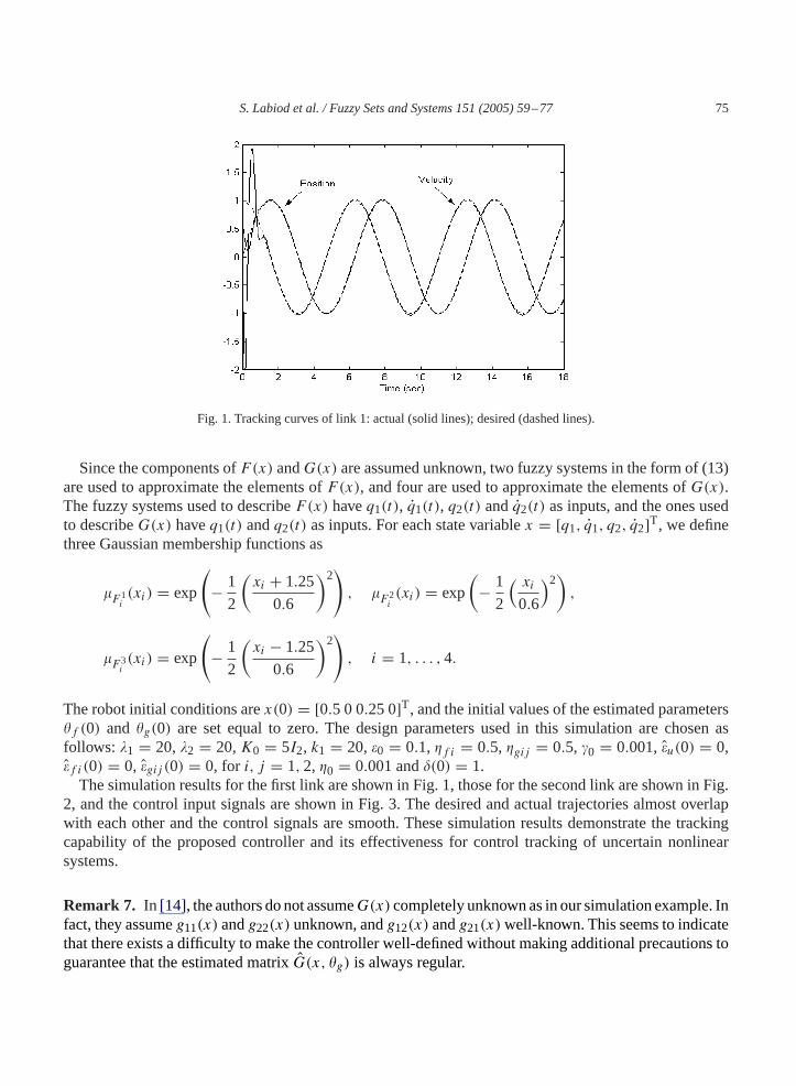
Fig. 1. Tracking curves of link 1: actual (solid lines); desired (dashed lines).

Since the components ofF(x) andG(x) are assumed unknown, two fuzzy systems in the form of (13)are used to approximate the elements ofF(x), and four are used to approximate the elements ofG(x).The fuzzy systems used to describeF(x) haveq1(t), q1(t), q2(t) andq2(t) as inputs, and the ones usedto describeG(x) haveq1(t) andq2(t) as inputs. For each state variablex = [q1, q1, q2, q2]T, we definethree Gaussian membership functions as

�F 1i(xi) = exp

(− 1

2

(xi + 1.25

0.6

)2), �F 2

i(xi) = exp

(− 1

2

( xi

0.6

)2),

�F 3i(xi) = exp

(− 1

2

(xi − 1.25

0.6

)2), i = 1, . . . ,4.

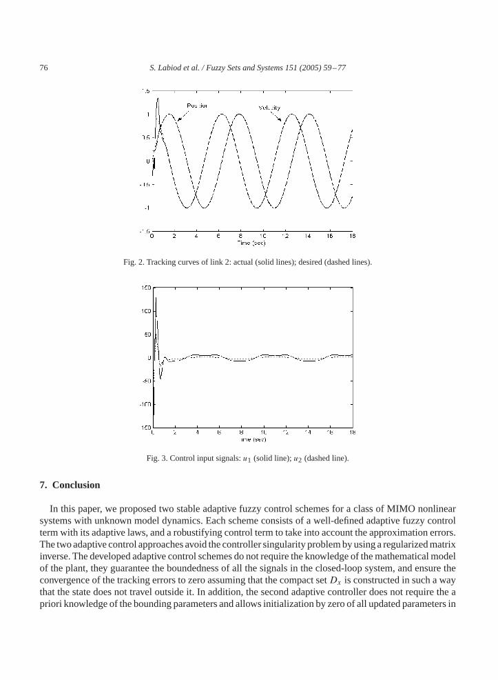
The robot initial conditions arex(0) = [0.5 0 0.25 0]T, and the initial values of the estimated parameters�f (0) and �g(0) are set equal to zero. The design parameters used in this simulation are chosen asfollows: �1 = 20,�2 = 20,K0 = 5I2, k1 = 20, �0 = 0.1, �f i = 0.5, �gij = 0.5, 0 = 0.001, �u(0) = 0,�f i(0) = 0, �gij (0) = 0, for i, j = 1,2, �0 = 0.001 and�(0) = 1.The simulation results for the first link are shown in Fig. 1, those for the second link are shown in Fig.

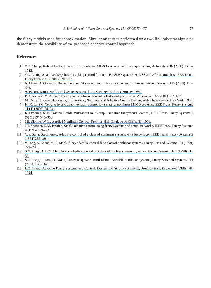
2, and the control input signals are shown in Fig. 3. The desired and actual trajectories almost overlapwith each other and the control signals are smooth. These simulation results demonstrate the trackingcapability of the proposed controller and its effectiveness for control tracking of uncertain nonlinearsystems.

Remark 7. In [14], the authors donot assumeG(x) completely unknownas in our simulation example. Infact, they assumeg11(x) andg22(x) unknown, andg12(x) andg21(x)well-known. This seems to indicatethat there exists a difficulty to make the controller well-defined without making additional precautions toguarantee that the estimated matrixG(x, �g) is always regular.

76 S. Labiod et al. / Fuzzy Sets and Systems 151 (2005) 59–77

Fig. 2. Tracking curves of link 2: actual (solid lines); desired (dashed lines).

Fig. 3. Control input signals:u1 (solid line);u2 (dashed line).

7. Conclusion

In this paper, we proposed two stable adaptive fuzzy control schemes for a class of MIMO nonlinearsystems with unknown model dynamics. Each scheme consists of a well-defined adaptive fuzzy controlterm with its adaptive laws, and a robustifying control term to take into account the approximation errors.The twoadaptive control approachesavoid the controller singularity problembyusinga regularizedmatrixinverse. The developed adaptive control schemes do not require the knowledge of themathematical modelof the plant, they guarantee the boundedness of all the signals in the closed-loop system, and ensure theconvergence of the tracking errors to zero assuming that the compact setDx is constructed in such a waythat the state does not travel outside it. In addition, the second adaptive controller does not require the apriori knowledge of the bounding parameters and allows initialization by zero of all updated parameters in

S. Labiod et al. / Fuzzy Sets and Systems 151 (2005) 59–77 77

the fuzzy models used for approximation. Simulation results performed on a two-link robot manipulatordemonstrate the feasibility of the proposed adaptive control approach.

References

[1] Y.C. Chang, Robust tracking control for nonlinear MIMO systems via fuzzy approaches, Automatica 36 (2000) 1535–1545.

[2] Y.C. Chang,Adaptive fuzzy-based tracking control for nonlinear SISO systems viaVSS andH∞ approaches, IEEE Trans.Fuzzy Systems 9 (2001) 278–292.

[3] N. Golea, A. Golea, K. Benmahammed, Stable indirect fuzzy adaptive control, Fuzzy Sets and Systems 137 (2003) 353–366.

[4] A. Isidori, Nonlinear Control Systems, second ed., Springer, Berlin, Germany, 1989.[5] P. Kokotovic, M. Arkac, Constructive nonlinear control: a historical perspective, Automatica 37 (2001) 637–662.[6] M. Krstic, I. Kanellakopoulos, P. Kokotovic, Nonlinear andAdaptive Control Design,Weley Interscience, NewYork, 1995.[7] H.-X. Li, S.C. Tong, A hybrid adaptive fuzzy control for a class of nonlinear MIMO systems, IEEE Trans. Fuzzy Systems

11 (1) (2003) 24–34.[8] R. Ordonez, K.M. Passino, Stable multi-input multi-output adaptive fuzzy/neural control, IEEE Trans. Fuzzy Systems 7

(3) (1999) 345–353.[9] J.E. Slotine, W. Li, Applied Nonlinear Control, Prentice-Hall, Englewood Cliffs, NJ, 1991.[10] J.T. Spooner, K.M. Passino, Stable adaptive control using fuzzy systems and neural networks, IEEE Trans. Fuzzy Systems

4 (1996) 339–359.[11] C.Y. Su, Y. Stepanenko, Adaptive control of a class of nonlinear systems with fuzzy logic, IEEE Trans. Fuzzy Systems 2

(1994) 285–294.[12] Y. Tang, N. Zhang,Y. Li, Stable fuzzy adaptive control for a class of nonlinear systems, Fuzzy Sets and Systems 104 (1999)

279–288.[13] S.C. Tong, Q. Li, T. Chai, Fuzzy adaptive control of a class of nonlinear systems, Fuzzy Sets and Systems 101 (1999) 31–

39.[14] S.C. Tong, J. Tang, T. Wang, Fuzzy adaptive control of multivariable nonlinear systems, Fuzzy Sets and Systems 111

(2000) 153–167.[15] L.X. Wang, Adaptive Fuzzy Systems and Control: Design and Stability Analysis, Prentice-Hall, Englewood Cliffs, NJ,

1994.