Embed Size (px)
Citation preview
DISS. ETH No. 17447
ACCURATE DOMAIN TRUNCATION TECHNIQUES FOR
TIME-DOMAIN CONFORMAL METHODS
A dissertation submitted to
ETH ZURICH
for the degree of
Doctor of Sciences
presented by
KRISHNASWAMY SANKARAN
M. Sc., Universitat Fridericiana Karlsruhe (TH), Germany
born October 10, 1980
citizen of Republic of India
accepted on the recommendation of
Prof. Dr. R. Vahldieck, examiner
Prof. Dr. W. J. R. Hoefer, co-examiner
Dr. C. Fumeaux, co-examiner
2007


It moves and It moves not; It is far and likewise near.It is inside all this and It is outside all this.
– Isa Upanisad


Abstract
This thesis is the product of research work carried out in the Laboratory for Elec-tromagnetic Fields and Microwave Electronics at ETH Zurich, Switzerland. Thefocus of this research is to develop accurate computational domain truncationtechniques for conformal time-domain methods. Due to the finite nature of avail-able resources, for example, computer memory, simulation time, etc., the compu-tational domain should also be finite and hence, the numerical methods requirevery accurate computational domain truncation techniques. In many cases, theaccuracy of these truncation techniques have a significant impact on the quality ofthe computed results. Therefore, the objective is to develop boundary truncationtechniques which can mimic infinite computational space. In practice, however,there exists a significant amount of reflection at the outer boundary of the maincomputational domain. Various techniques for reducing this non-physical reflec-tion have been developed during the last couple of decades which are generallyclassified as absorbing boundary conditions (ABC). All these ABCs perform ac-curately for one particular case for which they were optimized for. Moreover,the performance of these ABCs depend on the order of the truncation error interms of their Taylor series approximation. Higher order ABCs also require largecomputational efforts. Hence, there is a trade-off between the performance andthe computational efforts. The idea of developing an accurate ABC which canperfectly absorb all outgoing radiations with practically negligible reflection re-mained a long term dream until the introduction of the perfectly matched layer(PML) technique in 1994 by Berenger in the framework of the FDTD method.
The choice of conformal time-domain method in this research is mainly due tothe range of flexibility and accuracy attainable for a very detailed modelling ofelectromagnetic problems. The inherent limitations of the classical methods likethe FEM and FDTD methods motivate the choice of a non-mainstream methodnamely, the finite-volume time-domain (FVTD) method, which belongs to theclass of conformal time-domain methods. The concept of the FVTD methodoriginates from the field of computational fluid dynamics (CFD). The FVTD
i

ii ABSTRACT
method can employ unstructured spatial discretization similar to the FEM withan additional possibility of avoiding the limitations of the FEM (for example,frequency-domain or implicit time-update formulations). In other words, a sim-ple explicit time-update scheme similar to the FDTD method is possible in theFVTD framework. The FVTD method thus selectively combines the powerful at-tributes of the FEM (unstructured spatial discretization) with that of the FDTDmethod (explicit time-update formulation). In addition to the above mentionedfeatures, the FVTD method facilitates multi-scaling in a natural way allowingvery detailed modelling of electromagnetic structures. Furthermore, the methodalso enables to accurately model structures with a high dielectric-contrast andcurved geometries.
Prior to the present research, the most well-known ABC technique for theFVTD framework was the first-order accurate Silver-Muller ABC (SM-ABC)which is optimal only for normal incident outgoing waves. In addition, becauseof the mathematical complexity of the FVTD method, there was practicallyno investigation related to the PML techniques in the FVTD framework. Asthe performance of the boundary conditions have a significant influence on thecomputed results, these domain truncation techniques increase the level of ac-curacy attainable in comparison to predominantly used SM-ABC technique forthe FVTD method. In comparison with the SM-ABC, there is a significant in-crease in the computational effort to model the PML techniques; however, thisincrease can be compensated by the decrease in the effective computational do-main size. There exists a fundamental need for having a substantial distancebetween the scatterer or radiating structure and the truncation boundary in thecase of the SM-ABC technique. This is due to the fact that the SM-ABC isoptimized only for normal angle of incidence and its performance degrades dras-tically at off-normal angles. On the contrary, there are no such requirements inthe case of PML techniques because PMLs are theoretically reflectionless andpractically well-absorbing boundary truncation techniques for all incident anglesand hence, can be placed very close to the scatterering or radiating structures.In other words, the increased computational effort of the PML technique can becompensated by placing it very close to the scatterer or radiating structure.
The focus of this thesis is to investigate various PML and to develop accuratedomain truncation techniques in the FVTD framework. At the same time, this

ABSTRACT iii
thesis creates an organisation among various existing PML techniques based ontheir analytical formulation and theoretical relationship. This research work alsoaddresses the broadband behaviour of perfectly matched absorber techniques andsystematically validates the efficiency, performance and accuracy of the PMLtechniques for the FVTD simulation. Furthermore, a radial perfectly matchedabsorber model for accurate modelling of two-dimensional elongated geometriesis presented and extended to three-dimensional problems using the sphericalabsorber technique. Although the results presented in this research work wereobtained employing the FVTD method, the models analyzed can be naturallygeneralized to other conformal time-domain methods.

iv

Zusammenfassung
Diese Dissertation stellt das Ergebnis einer Forschungsarbeit dar, die am Insti-tut fur Feldtheorie und Hochstfrequenztechnik, ETH Zurich, durchgefuhrt wur-de. Der Forschungsschwerpunkt ist die Entwicklung einer exakten reflexionsfreienBegrenzung des Rechenbereiches fur konforme Zeitbereichmethoden. Infolge derbegrenzten Natur der Rechenressourcen (z.B. Speicher, Rechenzeit) muss derRechenbereich ebenfalls endlich sein, und deshalb braucht jede numerische Me-thode genaue Techniken um den Rechenbereich reflexionsfrei zu begrenzen. Invielen Fallen hat die Qualitat der ausseren Randbedingungen einen bedeutenderEinfluss auf die Genauigkeit der Rechenergebnisse. Das Ziel ist folglich eine Be-grenzung des Rechenbereiches zu entwickeln, die eine unendliche Ausdehnung desRaumes nachbildet. In der Praxis jedoch konnen bedeutende Reflexionen von denausseren Randbedingungen beobachtet werden. Verschiedene Methoden wurdenwahrend den letzten Jahrzehnten entwickelt, um diese unphysikalische Reflexio-nen zu reduzieren. Diese Methoden werden in Englisch als ‘Absorbing BoundaryConditions’ (ABC) bezeichnet. Alle ABC sind fur besondere Einfallsrichtungenoptimiert und arbeiten nur in bestimmten Fallen mit hoher Genauigkeit. Daruberhinaus hangt die Effizienz dieser ABC von der Naherungsordnung, d.h. von derAnzahl betrachteter Terme in ihrer Taylorentwicklung ab. Eine ABC mit hoherOrdnung wird aber auch hohe Rechenressourcen verlangen. Deshalb ist ein Kom-promiss zwischen der Genauigkeit und dem Rechenaufwand notig. Die Idee furdie Entwicklung einer genauen ABC, die fast perfekt reflexionsfrei alle abgestrahl-ten Wellen absorbiert, ist lange eine Vision geblieben. Dies anderte sich 1994 mitder Einfuhrung der Perfectly Matched Layer (PML) Technik von Berenger imRahmen der Finite-Differenzen Methode im Zeitbereich (FDTD).
Die wahl einer konformen Zeitbereichsmethode im Rahmen dieser Forschungs-arbeit ist motiviert durch die grosse Flexibilitat und Genauigkeit, die in dieserWeise fur sehr detaillierte elektromagnetische Probleme erreicht werden kann. Dieinharente Beschrankungen klassischer Methoden wie FEM und FDTD motiviertdie Erforschung weniger etablierten Methoden, wie zum Beispiel die Zeitbereich
v

vi ZUSAMMENFASSUNG
Finite-Volumen Methode (FVTD), die zur Klasse der konformen Zeitbereichsme-thoden gehort. Das FVTD-Konzept stammt aus dem Fachbereich der Rechen-gestutzten Fluiddynamik (Computational Fluid Dynamics, CFD). Die FVTD-Methode kann wie FEM eine unstrukturierte Raum diskretisierung benutzen, sievermeidet aber die Beschrankungen der FEM zum Frequenzbereich oder implizi-ten Zeititeration. In anderen Worten konnen im Rahmen der FVTD-Methodeeinfache Update-Gleichungen hergeleitet werden, wie fur FDTD. Die FVTD-Methode kombiniert dann selektiv die Starken der FEM (unstrukturierte Raum-diskretisierung) mit denen der FDTD-Methode (explizite zeitliche Update For-mulierung). Zusatzlich zu den erwahnten Merkmalen, kann die FVTD MethodeMulti-Skala Probleme sehr naturlich behandeln, was ausserst detaillierte Modelleelektromagnetischer Strukturen ermoglicht. Weiter erlaubt die Methode genaueModellierungen von Strukturen mit hohem dielektrischem Kontrast und gewolbteGeometrien.
Vor dieser Forschungsarbeit war die meistbekannte ABC-Technik im Rahmender FVTD-Methode die erste Ordnung Silver-Muller ABC (SM-ABC). Diese Me-thode ist nur optimal fur einen senkrechter Einfall auf der ausseren Begrenzungdes Rechenbereiches. Wegen der mathematischen Komplexitat gab es praktischkeine Untersuchungen der PML im Rahmen der FVTD-Methode. Da die Ge-nauigkeit der Randbedingungen einen signifikanten Einfluss auf die berechnetenResultate hat, kann eine PML-Rechenbereichbegrenzung die Genauigkeit der ge-samten Simulation erhohen, im Vergleich mit Resultaten die mit der uberwiegendangewandten SM-ABC-Technik erhalten werden. Der Rechenaufwand der PMLBegrenzung ist im Vergleich mit der SM-ABC Technik viel bedeutender, kannaber durch die Reduktion der Rechenbereichgrosse kompensiert werden. Im Fallder SM-ABC muss eine betrachtliche Distanz zwischen dem strahlenden oderstreuenden Korper und der ausseren Begrenzung vorhanden sein, um annaherndsenkrechte Einfallsbedingungen zu erreichen. Der Grund ist, dass SM-ABC nurfur den senkrechten Einfall exakt ist und die Genauigkeit drastisch reduziertwird, wenn der Einfallwinkel grosser wird. Dem gegenuber existieren solche Be-dingungen nicht fur den Fall der PML-Techniken: Die PML ist theoretisch nahezureflexionsfrei, und in der Praxis wird mit PML fur alle Einfallswinkel eine sehrhohe Dampfung erreicht, so dass die aussere Begrenzung sehr nah an den Strah-ler platziert werden kann. In anderen Worten kann der zusatzliche Aufwand der
ZUSAMMENFASSUNG vii
PML durch Reduktion des Rechenbereiches kompensiert werden.In diesem Zusammenhang bildet die Untersuchung verschiedener PML-Typen
zur Entwicklung genaueren reflexionsfreie Randbedingungen im Rahmen derFVTD-Methode den Schwerpunkt dieser Dissertation. Gleichzeitig werden Be-ziehungen zwischen unterschiedlichen PML-Implementierungen aufgrund ihreranalytischen Formulierung und Genauigkeit definiert. Diese Forschungsarbeit un-tersucht weiter das breitbandige Verhalten der PML-Techniken und validiert sy-stematisch ihre Effizienz und Genauigkeit. Weiter wird ein radiales PML-Modellentwickelt um zweidimensionale Geometrien zu simulieren. Dieses Model ist furdrei Dimensionen in der Form von kugelschalenformigen PML erweitert worden.Alle erhaltenen Resultate dieser Arbeit wurden im Rahmen der FVTD-Methodeerzielt. Die entwickelten Modelle konnen naturgemass fur andere konforme Me-thoden im Zeitbereich erweitert werden.

viii
Contents
Acknowledgment
1 Introduction 1
1.1 Computational Electromagnetics (CEM) . . . . . . . . . . . . . . 11.2 Conformal Time-Domain Methods: A Finite-Volume Time-Domain
(FVTD) Approach . . . . . . . . . . . . . . . . . . . . . . . . . . 21.3 Perfectly Matched Layer (PML) for FVTD Method . . . . . . . . 31.4 Overview of this thesis . . . . . . . . . . . . . . . . . . . . . . . . 41.5 Chapter Organisation . . . . . . . . . . . . . . . . . . . . . . . . 6
2 Conservation Laws and Conformal Modelling 7
2.1 Maxwell System . . . . . . . . . . . . . . . . . . . . . . . . . . . 72.2 Theory of Conservation Law . . . . . . . . . . . . . . . . . . . . . 112.3 Maxwell System as a Conservation Law . . . . . . . . . . . . . . 142.4 Hyperbolicity and Charateristics . . . . . . . . . . . . . . . . . . 162.5 Need for Conformal Time-Domain Methods . . . . . . . . . . . . 182.6 A FVTD Approach . . . . . . . . . . . . . . . . . . . . . . . . . . 20
2.6.1 Finite Volume: Definitions . . . . . . . . . . . . . . . . . . 202.6.2 FVTD Formulation of the Maxwell System . . . . . . . . 222.6.3 Riemann Problem and Superposition of Waves . . . . . . 23
2.7 Flux Definitions . . . . . . . . . . . . . . . . . . . . . . . . . . . . 272.7.1 Tangential Continuity Condition . . . . . . . . . . . . . . 282.7.2 Dielectric Interface Condition . . . . . . . . . . . . . . . . 282.7.3 Perfect Electric Conductor (PEC) Boundary Condition . 292.7.4 Perfect Magnetic Conductor (PMC) Boundary Condition 302.7.5 Absorbing Boundary Condition (ABC): Silver-Muller ABC 30
2.8 Spatial and Temporal Discretization Procedure . . . . . . . . . . 302.8.1 Stability and CFL Limit . . . . . . . . . . . . . . . . . . . 33
ix

x CONTENTS
3 Split-Field Based Finite-Volume Absorber Model 35
3.1 Introduction . . . . . . . . . . . . . . . . . . . . . . . . . . . . . . 353.2 FVTD–B-PML Model . . . . . . . . . . . . . . . . . . . . . . . . 36
3.2.1 Definition of Flux Functions . . . . . . . . . . . . . . . . . 373.2.2 Split-field (Ezy) Flux Update . . . . . . . . . . . . . . . . 393.2.3 Model problem – Parallel-plate Waveguide . . . . . . . . . 43
3.3 Numerical Experiments . . . . . . . . . . . . . . . . . . . . . . . 443.3.1 B-PML Profile . . . . . . . . . . . . . . . . . . . . . . . . 453.3.2 B-PML Thickness . . . . . . . . . . . . . . . . . . . . . . 483.3.3 Convergence Analysis . . . . . . . . . . . . . . . . . . . . 483.3.4 Broadband Characteristics . . . . . . . . . . . . . . . . . 493.3.5 Numerical Stability . . . . . . . . . . . . . . . . . . . . . . 503.3.6 Angular Dependence of Performance . . . . . . . . . . . . 503.3.7 Example Problem . . . . . . . . . . . . . . . . . . . . . . 51
3.4 Hybrid Domain Truncation: B-PML + SM-ABC . . . . . . . . . 523.4.1 Internal and Boundary Interface Treatments . . . . . . . 523.4.2 PML Boundary Condition . . . . . . . . . . . . . . . . . . 53
3.5 Pure and Hybrid Techniques . . . . . . . . . . . . . . . . . . . . 543.6 Conclusions . . . . . . . . . . . . . . . . . . . . . . . . . . . . . . 57
4 Material Based FVTD Absorber Model 59
4.1 Introduction . . . . . . . . . . . . . . . . . . . . . . . . . . . . . . 594.2 FVTD - Modified Lorentz Material Model . . . . . . . . . . . . . 604.3 Numerical Implementation . . . . . . . . . . . . . . . . . . . . . . 63
4.3.1 Spatial and Temporal Discretizations . . . . . . . . . . . . 634.3.2 Damping and Coupling Coefficient . . . . . . . . . . . . . 64
4.4 Numerical Experiment . . . . . . . . . . . . . . . . . . . . . . . . 644.4.1 Test Problem: Definition . . . . . . . . . . . . . . . . . . 644.4.2 Absorber Performance versus Angle of Incident Radiation 654.4.3 Absorber Performance versus Absorber Thickness . . . . 67
4.5 Conclusions . . . . . . . . . . . . . . . . . . . . . . . . . . . . . . 69
5 Unified FVTD Absorber Modelling 71
5.1 Introduction . . . . . . . . . . . . . . . . . . . . . . . . . . . . . . 715.2 Non-Maxwellian Absorbers . . . . . . . . . . . . . . . . . . . . . 72
CONTENTS xi
5.2.1 Berenger PML - (B-PML) . . . . . . . . . . . . . . . . . . 725.3 Maxwellian Absorbers . . . . . . . . . . . . . . . . . . . . . . . . 73
5.3.1 Modified Lorentz Material-based PML - (M-PML) . . . . 735.3.2 Generalized Theory based PML - (GT-PML) . . . . . . . 735.3.3 Complex Frequency Shifted PML - (CFS-PML) . . . . . . 75
5.4 Numerical Performance Comparison . . . . . . . . . . . . . . . . 765.5 Conclusion . . . . . . . . . . . . . . . . . . . . . . . . . . . . . . 78
6 Radial Perfectly Matched Absorber Modelling 79
6.1 Introduction . . . . . . . . . . . . . . . . . . . . . . . . . . . . . . 796.2 Radial Finite-Volume Maxwellian Absorber . . . . . . . . . . . . 80
6.2.1 Radial Anisotropy: Rotated Coordinate Analysis . . . . . 816.2.2 Definition of Anisotropic Losses: Comparison to Standard
Approach . . . . . . . . . . . . . . . . . . . . . . . . . . . 816.2.3 Field Update Equations . . . . . . . . . . . . . . . . . . . 826.2.4 Numerical Experiments . . . . . . . . . . . . . . . . . . . 85
6.3 Broadband Performance Analysis . . . . . . . . . . . . . . . . . . 896.4 Influence of the Radius of Curvature . . . . . . . . . . . . . . . . 93
6.4.1 Uniaxial Absorber: Limiting Case of Radial Absorber . . 936.5 Numerical Experiment: Horn Antenna . . . . . . . . . . . . . . . 946.6 Extension to 3D Geometries: Concept . . . . . . . . . . . . . . . 976.7 Conclusion . . . . . . . . . . . . . . . . . . . . . . . . . . . . . . 98
7 3D - Spherical FVTD-PML 101
7.1 Introduction . . . . . . . . . . . . . . . . . . . . . . . . . . . . . . 1017.2 3D Spherical PML Models: Theory . . . . . . . . . . . . . . . . . 101
7.2.1 Definition of Rotational Matrix . . . . . . . . . . . . . . . 1027.2.2 3D FVTD Spherical PML Update Equations . . . . . . . 1037.2.3 Implementation Issues . . . . . . . . . . . . . . . . . . . . 108
7.3 Numerical Examples . . . . . . . . . . . . . . . . . . . . . . . . . 1087.3.1 Waveguide Truncation: Spherical PML with Infinite Ra-
dius of Curvature . . . . . . . . . . . . . . . . . . . . . . . 1097.3.2 Spherical Domain with a Point-Source . . . . . . . . . . . 1107.3.3 Mutual Coupling between Archimedian Spiral Antennas . 113
7.4 Conclusion . . . . . . . . . . . . . . . . . . . . . . . . . . . . . . 115

xii CONTENTS
8 Conclusion & Outlook 119
Bibliography 123
List of Publications 131
Curriculum Vitae 135
List of Figures
1.1 Features of FVTD Method. Left: Multi-scaling for efficient mod-elling of electromagnetic structures. Right: Accurate modelling ofstructures with high dielectric-contrast and curved boundaries. . 3
1.2 Fundamental requirements of perfect absorber. . . . . . . . . . . 51.3 Positioning of the research focus. . . . . . . . . . . . . . . . . . . 5
2.1 Graphical illustration of Maxwell curl equations. . . . . . . . . . 82.2 An example for the computational domain of interest Ω with the
enclosing boundary ∂Ω shown along with the normal vector at asample point on ∂Ω with components nx and ny along the x andy axes, respectively. . . . . . . . . . . . . . . . . . . . . . . . . . 12
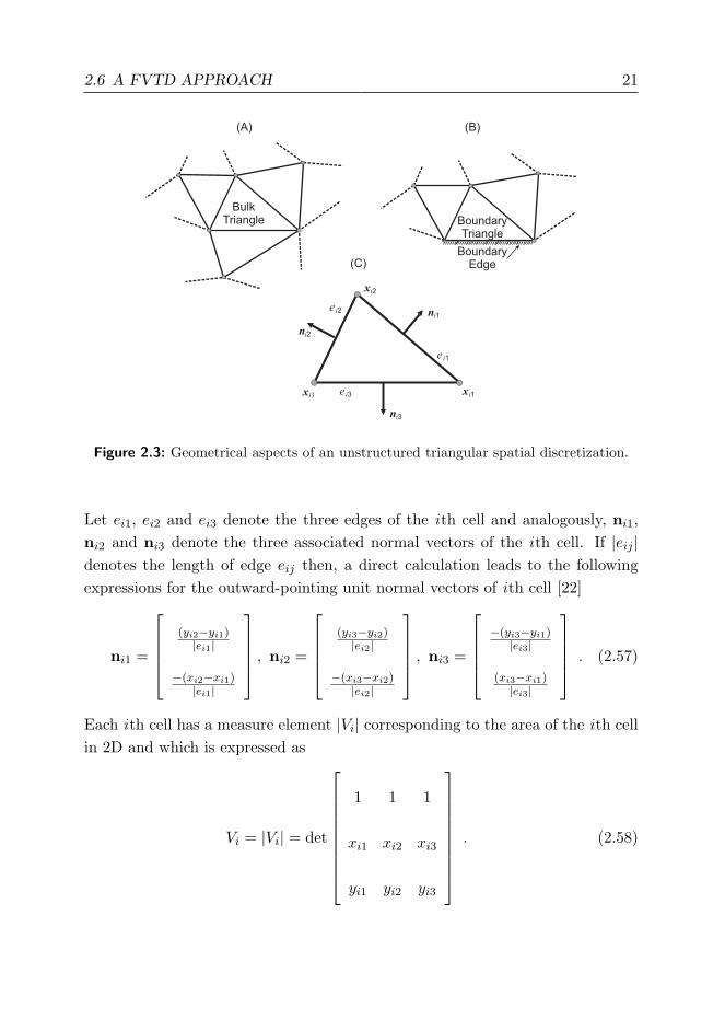
2.3 Geometrical aspects of an unstructured triangular spatial discretiza-tion. . . . . . . . . . . . . . . . . . . . . . . . . . . . . . . . . . . 21
2.4 Discontinuity in field values in the adjacent cells in the computa-tional domain. The field vector state is denoted as U− for xn < 0and U+ for xn > 0. The LHS and RHS of the edge is denoted as-© and +©, respectively. . . . . . . . . . . . . . . . . . . . . . . . 24
2.5 Characteristics plot for the Maxwell system . . . . . . . . . . . . 252.6 Flux-splitting scheme based on forward and reverse propagating
fields at each edge. Left and right approximations are derivedbased on the information from the left and right neighbours, re-spectively. Corresponding velocities of information propagationalso indicated. . . . . . . . . . . . . . . . . . . . . . . . . . . . . . 28
2.7 Flux-splitting approach to approximate the left and right field val-ues at each edge during each time step. The left and right field val-ues contribute to the outgoing and incoming fluxes, respectively.The left side of the edge is marked +© and the right side is markedwith -©. . . . . . . . . . . . . . . . . . . . . . . . . . . . . . . . 31
xiii

xiv LIST OF FIGURES
2.8 Piecewise constant approximation strategy used in Godunov schemewhich leads to a 1st order accurate method. . . . . . . . . . . . . 32
2.9 Piecewise linear approximation strategy used in MUSCL approachwhich leads to a second order accurate method. . . . . . . . . . . 33
2.10 Second-order accurate Lax-Wendroff scheme using a predictor andcorrector scheme. The time-step for the predictor step is half thatof standard Euler scheme (2.63). The corrector time-step is equalto that of standard Euler scheme. . . . . . . . . . . . . . . . . . . 34
3.1 Split-field flux calculation by 2D to 1D transformation (Riemannproblem). . . . . . . . . . . . . . . . . . . . . . . . . . . . . . . . 39
3.2 Solution to 1D Riemann problem using Rankine–Hugoniot jumprelation. . . . . . . . . . . . . . . . . . . . . . . . . . . . . . . . . 40
3.3 Model domain used for characterizing B-PML. . . . . . . . . . . 433.4 Structured-type and unstructured-type triangular meshes. . . . . 453.5 Numerical reflection coefficient (dB) as a function of maximum
PML conductivity σ0 for different profiles. . . . . . . . . . . . . . 463.6 Numerical reflection coefficient (dB) as a function of theoretical
reflection coefficient (dB) for different profiles. . . . . . . . . . . . 473.7 Numerical reflection coefficient (dB) as a function of theoretical
reflection coefficient (dB) for different B-PML thickness (dpml).The spatial discretization is constant (λ/10). . . . . . . . . . . . 48
3.8 Numerical reflection coefficient (dB) as a function of theoreticalreflection coefficient (dB) for different spatial discretization. . . . 49
3.9 Energy inside B-PML model as a function of time period. . . . . 503.10 Comparison of numerical reflection coefficient (dB) for different
angles of plane wave incidence for B-PML and SM-ABC. . . . . . 513.11 Different boundary types illustrated using a parallel-plate waveg-
uide example. . . . . . . . . . . . . . . . . . . . . . . . . . . . . . 523.12 Parallel-plate waveguide example illustrating different possibilities
of employing PEC or SM-ABC based B-PML truncation. . . . . 543.13 Broadband performance analysis of pure and hybrid domain trun-
cation techniques at normal incidence. . . . . . . . . . . . . . . . 553.14 Broadband performance analysis of pure and hybrid domain trun-
cation techniques at 45 degree angle of incidence. . . . . . . . . . 56
LIST OF FIGURES xv
4.1 Comparison between FDTD and FVTD Maxwellian absorber fieldorientation model. . . . . . . . . . . . . . . . . . . . . . . . . . . 63
4.2 Models for calculating reflection coefficient. Top: Reference model.Bottom: Test model. . . . . . . . . . . . . . . . . . . . . . . . . . 65
4.3 Sample problem for reflection coefficient analysis of the FVTD-Maxwellian absorber corresponding to 30 degree angle of incidence. 66
4.4 Angular response of the FVTD-Maxwellian absorber for differentmaterial loss parameter ζ0. . . . . . . . . . . . . . . . . . . . . . 66
4.5 Effect of absorber thickness on its performance at three differentangles of incidence for material loss parameter ζ0 = 1ω. . . . . . 67
4.6 Effect of absorber thickness on its performance at three differentangles of incidence for material loss parameter ζ0 = 2ω. . . . . . 68
4.7 Effect of absorber thickness on its performance at three differentangles of incidence for material loss parameter ζ0 = 8ω. . . . . . 68
5.1 Broadband performance of different FVTD-PML models in com-parison with theoretical value in a parallel-plate-waveguide. . . . 77
6.1 Graphical illustration of radial anisotropy using coordinate trans-formation by rotation. . . . . . . . . . . . . . . . . . . . . . . . . 81
6.2 Left: Three different kinds of uniaxial medium used in rectangularPML. Right: Concept of local to global transformation used inradial absorber theory. Corresponding directions of anisotropyare given with the damping coefficient. Dotted Lines: Commonarea of the computational domain. . . . . . . . . . . . . . . . . . 82
6.3 Model problem illustrating the test and reference domains. Thetest model of radius approximately 3.33λ is truncated using thefinite-volume Maxwellian absorber of thickness dabs = 0.5λ. . . . 86
6.4 Different angles of incidence at the FS-A interface based on sourcelocation. . . . . . . . . . . . . . . . . . . . . . . . . . . . . . . . . 86
6.5 Comparison of results of numerical error using Silver-Mueller ABCand finite-volume Maxwellian absorber for the centred-source sce-nario. . . . . . . . . . . . . . . . . . . . . . . . . . . . . . . . . . 87

xvi LIST OF FIGURES
6.6 Comparison of results of numerical error using Silver-Mueller ABCand finite-volume Maxwellian absorber for the off-centred-sourcescenario. . . . . . . . . . . . . . . . . . . . . . . . . . . . . . . . . 88
6.7 Comparison of numerical reflection at a test point due to the finite-volume Maxwellian absorber and SM-ABC for the example sce-nario shown in the inset. . . . . . . . . . . . . . . . . . . . . . . . 89
6.8 Electric field plot at different time stamps for a centred axial linesource excited by a broadband sine-modulated Gaussian pulse. . 90
6.9 Electric field plot at different time stamps for an off-centred axialline source excited by a broadband sine-modulated Gaussian pulse. 91
6.10 Normalized energy inside the domain as a function of time. . . . 92
6.11 Numerical reflection at a test point near the domain centre forboth centred and off-centred source scenarios. . . . . . . . . . . . 93
6.12 Left: Cylindrical domain truncation. Right: Waveguide trunca-tion emphasizing that the uniaxial absorber is a limiting case ofradial absorber with infinite radius of curvature. . . . . . . . . . 94
6.13 Waveguide truncation showing the convergence of the radial ab-sorber with increasing radius of curvature rC towards the uniax-ial absorber model. The performance of the first-order accurateSM-ABC is also shown as a comparison. The angle of incidencecorresponding to each frequency is also indicated on the upperhorizontal scale. The theoretical results at each angle is computedsuch that a PML reflection coefficient of −70 dB is achieved atnormal incidence. . . . . . . . . . . . . . . . . . . . . . . . . . . . 95
6.14 Computational Domain consisting of 2D horn-antenna with differ-ent rC. The NF-FF contour used to compute antenna radiationpattern is shown. . . . . . . . . . . . . . . . . . . . . . . . . . . . 96
LIST OF FIGURES xvii
6.15 Reflections from the radial absorber of different radii used to trun-cate the domain consisting of radiating horn-antenna excited byfirst-order TE10 mode. The free-space – absorber interface is de-picted in the case of rC = 80 mm and rC = 100 mm. In the othercases the free-space – radial absorber interface are further awayand therefore, not shown in the two bottom plots. The area out-side the dashed circles corresponds to the radial PML and showsa large difference with respect to the reference because of the ab-sorption in the radial PML. . . . . . . . . . . . . . . . . . . . . . 97
6.16 Horn-antenna radiation pattern at 10 GHz using radial absorberof different radii. The results shown nearly same results for themain-lobe of the antenna. Differences are observable in the side-lobes which are well below −40 dB. Convergence in the result isnoticed as rC increases. . . . . . . . . . . . . . . . . . . . . . . . 98
7.1 A typical application of spherical domain truncation. Left: SM-ABC. Right: PML . . . . . . . . . . . . . . . . . . . . . . . . . . 103
7.2 Numerical return-loss S11(f) of a WR90 rectangular waveguidetruncated by a 15 mm thick uniaxial PML for different theoreticalreflection-coefficent computed at normal incidence Γ0 = Γ(γ = 0).The theoretical values are computed according to (7.34). . . . . . 109
7.3 Snapshots of the z -component of the electric field radiated from aninfinitesimal point-source in spherical domain at two different timestamps. Left: First-order SM-ABC truncation. Right: SphericalPML truncation. The point-source location is shown as a circlewith a dot. The location of the field-sensor used to compute thereflection at a test point is depicted as a square with a cross. At t1,the incident pulse is still visible, whereas at t2, the incident pulsehas already left the computational domain and only the numericalreflections from the boundaries are observed. . . . . . . . . . . . 111

xviii LIST OF FIGURES
7.4 Left: Electric field amplitude as a function of time recorded at thefield-sensor location marked as a square with a cross. The incidentpulse is visible around t1 and the reflected pulse around t2 corre-sponding to the time-stamps in Fig. 7.3. Right: Saturated greyscale image showing very low-level reflections from the sphericalPML at t2. . . . . . . . . . . . . . . . . . . . . . . . . . . . . . . 112
7.5 Tilted configuration of two cavity-backed Archimedean spiral an-tennas. A cut-open view of the RHS spiral shows part of its surfacemesh, feeding balun and the cavity. The illustration also shows thecut-through view of the whole computational domain denoting theradius of curvatures of SM-ABC (RABC) and spherical absorber(RPML) truncations. . . . . . . . . . . . . . . . . . . . . . . . . . 114
7.6 Measured and computed antenna coupling parameter S21 of thetwo spiral antennas for the configuration shown in Fig. 7.5. Thecomputational domain is truncated using SM-ABC with differentradii of curvature RABC. . . . . . . . . . . . . . . . . . . . . . . . 115
7.7 Measured and computed antenna coupling parameter S21 of thetwo spiral antennas for the configuration shown in Fig. 7.5. Thecomputational domain is truncated using spherical absorber (FVTD-PML) with radius RABC = 98 mm and thickness of 17 mm. . . . 116

List of Acronyms and Abbreviations
Computational Methods
DGTD . . . . . . . . . . . . . . . . . . . . . . . . . . . . . . . . . Discontinuous-Galerkin Time-Domain
FDTD . . . . . . . . . . . . . . . . . . . . . . . . . . . . . . . . . . . . . . . . Finite-Difference Time-Domain
FEM . . . . . . . . . . . . . . . . . . . . . . . . . . . . . . . . . . . . . . . . . . . . . . . . . . Finite-Element Method
FIT . . . . . . . . . . . . . . . . . . . . . . . . . . . . . . . . . . . . . . . . . . . . . . Finite-Integration Technique
FVTD . . . . . . . . . . . . . . . . . . . . . . . . . . . . . . . . . . . . . . . . . . . Finite-Volume Time-Domain
TLM . . . . . . . . . . . . . . . . . . . . . . . . . . . . . . . . . . . . . . . . . . . . . . . Transmission Line Matrix
Computational Techniques and Schemes
ABC . . . . . . . . . . . . . . . . . . . . . . . . . . . . . . . . . . . . . . . . . . Absorbing Boundary Condition
CEM . . . . . . . . . . . . . . . . . . . . . . . . . . . . . . . . . . . . . . . . Computational ElectroMagnetics
CFD . . . . . . . . . . . . . . . . . . . . . . . . . . . . . . . . . . . . . . . . . . Computational Fluid Dynamics
CFS-PML . . . . . . . . . . . . . . . Complex Frequency Shifted Perfectly Matched Layer
DFT . . . . . . . . . . . . . . . . . . . . . . . . . . . . . . . . . . . . . . . . . Discrete Fourier Transformation
FFT . . . . . . . . . . . . . . . . . . . . . . . . . . . . . . . . . . . . . . . . . . . . . Fast Fourier Transformation
FS-A . . . . . . . . . . . . . . . . . . . . . . . . . . . . . . . . . . . . . . . . . . . . . . . . . . . . Free-space–Absorber
GT-PML . . . . . . . . . . . . . . . . . . . . . . General Theory based Perfectly Matched Layer
M-PML . . . . . . . . . . . . Modified Lorentz Material based Perfectly Matched Layer
MUSCL . . . . . . . . . Monotonic Upstream-centered Scheme for Conservation Laws
NFFF . . . . . . . . . . . . . . . . . . . . . . . . . . . . . . . . . . . . . . . . . . . . . . . . . . NearField-to-FarField
xix

xx LIST OF ACRONYMS
PEC . . . . . . . . . . . . . . . . . . . . . . . . . . . . . . . . . . . . . . . . . . . . . . . Perfect Electric Conductor
PMC . . . . . . . . . . . . . . . . . . . . . . . . . . . . . . . . . . . . . . . . . . . . . Perfect Magnetic Conductor
PML . . . . . . . . . . . . . . . . . . . . . . . . . . . . . . . . . . . . . . . . . . . . . . . . Perfectly Matched Layer
SM-ABC . . . . . . . . . . . . . . . . . . . . . . . . Silver-Muller Absorbing Boundary Condition
Standard Electromagnetic Terms
EM . . . . . . . . . . . . . . . . . . . . . . . . . . . . . . . . . . . . . . . . . . . . . . . . . . . . . . . . . . Electromagnetic
TEM . . . . . . . . . . . . . . . . . . . . . . . . . . . . . . . . . . . . . . . . . . . . . Transverse Electromagnetic
TE . . . . . . . . . . . . . . . . . . . . . . . . . . . . . . . . . . . . . . . . . . . . . . . . . . . . . . . . Transverse Electric
TM . . . . . . . . . . . . . . . . . . . . . . . . . . . . . . . . . . . . . . . . . . . . . . . . . . . . . . Transverse Magnetic
EMC . . . . . . . . . . . . . . . . . . . . . . . . . . . . . . . . . . . . . . . . . . Electromagnetic Compatibility
Mathematical Terms
BW . . . . . . . . . . . . . . . . . . . . . . . . . . . . . . . . . . . . . . . . . . . . . . . . . . . . . . . . . . . . . . BandWidth
FD . . . . . . . . . . . . . . . . . . . . . . . . . . . . . . . . . . . . . . . . . . . . . . . . . . . . . . . . Frequency-Domain
ODE . . . . . . . . . . . . . . . . . . . . . . . . . . . . . . . . . . . . . . . . . . Ordinary Differential Equation
PDE . . . . . . . . . . . . . . . . . . . . . . . . . . . . . . . . . . . . . . . . . . . . . Partial Differential Equation
TD . . . . . . . . . . . . . . . . . . . . . . . . . . . . . . . . . . . . . . . . . . . . . . . . . . . . . . . . . . . . . Time-Domain
1D . . . . . . . . . . . . . . . . . . . . . . . . . . . . . . . . . . . . . . . . . . . . . . . . . . . . . . . . . . . . . 1 Dimensional
2D . . . . . . . . . . . . . . . . . . . . . . . . . . . . . . . . . . . . . . . . . . . . . . . . . . . . . . . . . . . . . 2 Dimensional
3D . . . . . . . . . . . . . . . . . . . . . . . . . . . . . . . . . . . . . . . . . . . . . . . . . . . . . . . . . . . . . 3 Dimensional

LIST OF ACRONYMS xxi
Organizations and official terms
IEEE . . . . . . . . . . . . . . . . . . . . . . . . . Institute of Electrical and Electronics Engineers
IFH . . . . . . . . . . . . . Institut fur Feldtheorie und Hochstfrequenztechnik (German)
. . . Laboratory for Electromagnetic Fields and Microwave Electronics (English)
ACES . . . . . . . . . . . . . . . . . . . . . . . Applied Computational Electromagnetics Society
MTT-S . . . . . . . . . . . . . . . . . . . . . . . . . . . . Microwave Theory and Techniques Society
AP-S . . . . . . . . . . . . . . . . . . . . . . . . . . . . . . . . . . . . . . Antennas and Propagation Society
EuMW . . . . . . . . . . . . . . . . . . . . . . . . . . . . . . . . . . . . . . . . . . . . European Microwave Week
APMC . . . . . . . . . . . . . . . . . . . . . . . . . . . . . . . . . . . . Asia Pacific Microwave Conference
Miscellaneous
LHS . . . . . . . . . . . . . . . . . . . . . . . . . . . . . . . . . . . . . . . . . . . . . . . . . . . . . . . . . . . Left-hand side
RHS . . . . . . . . . . . . . . . . . . . . . . . . . . . . . . . . . . . . . . . . . . . . . . . . . . . . . . . . . . Right-hand side

xxii

Mathematical Notation
a Scalar
a,A Vector
nk Outward-pointing normal vector of kth face of a triangle or tetra-hedron
|Vi| Volume or area of ith tetrahedron or triangle respectively
|Sk| Surface area or length of kth face of a tetrahedron or trianglerespectively
[·]m×n Matrix with m rows and n columns
[1]m×m Unit square matrix with m rows and m columns
X,x Tensor
Re· Real-part of a complex-number ·
Im· Imaginary-part of a complex-number ·
∇ ×X Curl operation on a vector X
∇ ·X Divergence operation on a vector X
xxiii

xxiv MATHEMATICAL NOTATION
∂S Boundary line enclosing the surface S
dS Differential surface
S Surface area
∂V Surface enclosing the volume V
V Volume V
dV Differential volume
∂t Partial differential operator with respect to time t
∂x Partial differential operator with respect to spatial x coordinate
∂y Partial differential operator with respect to spatial y coordinate
∂z Partial differential operator with respect to spatial z coordinate
x, y, z Cartesian spatial coordinates
xr, yr, zr Rotated Cartesian spatial coordinates
E Electric field intensity vector
H Magnetic field intensity vector
D Electric displacement density vector
B Magnetic Flux density vector
P Polarization vector
M Magnetization vector

MATHEMATICAL NOTATION xxv
Ax, Ay, Az Cartesian components of vector A
U Combined electromagnetic vector (for example U = [Hx, Hy, Ez]T
where superscript T denotes matrix transpose)
F(U) Flux function of vector U
A Coefficient (material) matrix
A Projected coefficient matrix (A = n · A)
ε Permittivity of the medium
εr Relative permittivity of the medium
ε0 Permittivity of free-space
µ Permeability of the medium
µr Relative permeability of the medium
µ0 Permeability of free-space
χe Electric susceptibility
χm Magnetic susceptibility
σE Electric conductivity
σM Magnetic conductivity
σ PML loss term (σ ≡ σE/ε = σM/µ)

xxvi
1 Introduction
All the mathematical sciences are founded on relations betweenphysical laws and laws of numbers, so that the aim of exact scienceis to reduce the problems of nature to the determination of quantitiesby operations with numbers. – James Clark Maxwell, 1856
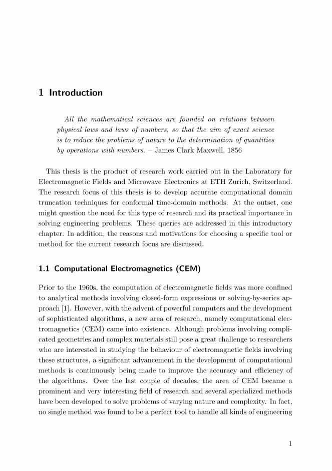
This thesis is the product of research work carried out in the Laboratory forElectromagnetic Fields and Microwave Electronics at ETH Zurich, Switzerland.The research focus of this thesis is to develop accurate computational domaintruncation techniques for conformal time-domain methods. At the outset, onemight question the need for this type of research and its practical importance insolving engineering problems. These queries are addressed in this introductorychapter. In addition, the reasons and motivations for choosing a specific tool ormethod for the current research focus are discussed.
1.1 Computational Electromagnetics (CEM)
Prior to the 1960s, the computation of electromagnetic fields was more confinedto analytical methods involving closed-form expressions or solving-by-series ap-proach [1]. However, with the advent of powerful computers and the developmentof sophisticated algorithms, a new area of research, namely computational elec-tromagnetics (CEM) came into existence. Although problems involving compli-cated geometries and complex materials still pose a great challenge to researcherswho are interested in studying the behaviour of electromagnetic fields involvingthese structures, a significant advancement in the development of computationalmethods is continuously being made to improve the accuracy and efficiency ofthe algorithms. Over the last couple of decades, the area of CEM became aprominent and very interesting field of research and several specialized methodshave been developed to solve problems of varying nature and complexity. In fact,no single method was found to be a perfect tool to handle all kinds of engineering
1
2 1 INTRODUCTION
problems. In many cases, the expertise of the user plays a crucial role in choosingthe most appropriate method for a given problem.
1.2 Conformal Time-Domain Methods: A Finite-Volume
Time-Domain (FVTD) Approach
In the world of computational science, two methods dealing with a volume spatialdiscretization approach gained substantial attention and momentum. These twomainstream methods, namely the finite-difference time-domain (FDTD) methodand the finite-element method (FEM) [2] were used for most, if not all, problems.The FDTD method is a well-known tool for many electrical engineers primar-ily due to its simplicity in implementation and understanding. In fact, this isthe main reason for the huge advancement of this method. However, the FDTDmethod in its classical formulation is limited to structured rectangular spatial dis-cretization, thereby inducing stair-casing errors when modelling complex curvedor inclined geometries.
On the other hand, the FEM gives maximum flexibility to model practicallyany kind of complex curved structures using unstructured spatial discretization.But, the FEM tools are used predominently in a frequency-domain formulationand this requires a separate simulation at each frequency to obtain broadbandresults. Furthermore, the increase in memory requirement is not proportional tonumber of cells in the computational domain. This means that if the numberof cells in the computational domain is increased by a factor two, the increasein memory requirement is much more than a factor two. The time-domain for-mulation of the FEM results in a global implicit time-updating scheme whichrequires global matrix-inversion at each time-step. Consequently, these implicittime-update formulations face a significant problem due to large computationalresource requirements.
For many broadband applications, methods cast in their time-domain formu-lation provide the desirable wide-band results in a single simulation run. As aresult of the increasing complexity of models as well as the inherent limitationsof the mainstream methods in terms of accuracy, flexibility and computationalrequirements, it has become important to develop novel methods which can effi-ciently handle at least some of these constraints.
The aforementioned limitations of the classical methods motivate the inves-
1.3 PERFECTLY MATCHED LAYER (PML) FOR FVTD METHOD 3
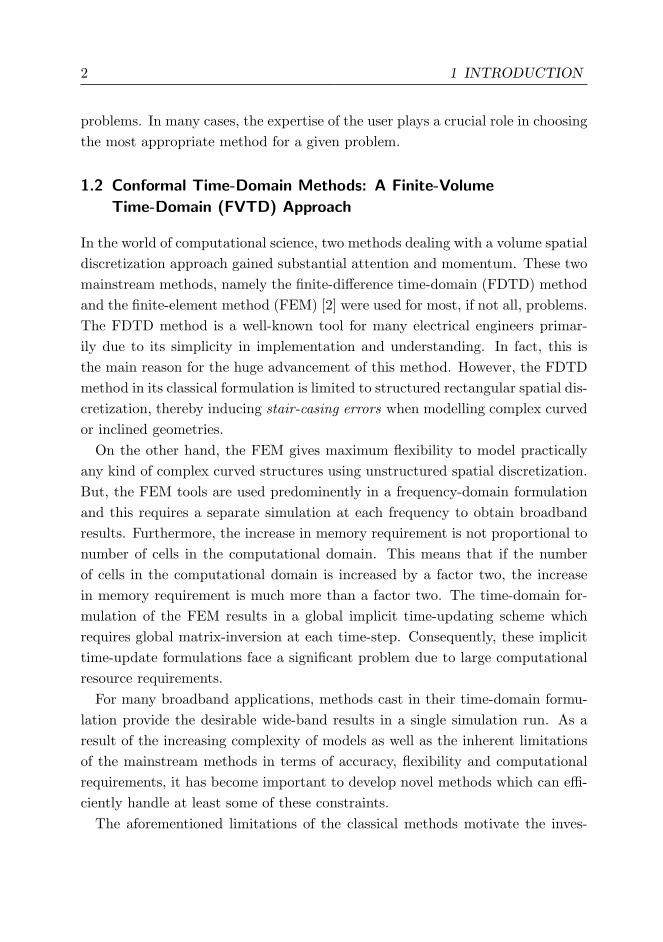
tigation of a non-mainstream method, namely the finite-volume time-domain(FVTD) method, which belongs to the class of conformal time-domain methods.The concept of the FVTD method originates from the field of computationalfluid dynamics (CFD). The FVTD method can employ unstructured spatial dis-cretization similar to the FEM with an additional possibility of avoiding thelimitations of the FEM (for example, frequency-domain or implicit time-updateformulations). In other words, a simple explicit time-update scheme similar to theFDTD method is possible in the FVTD framework. The FVTD method thusselectively combines the powerful attributes of the FEM (unstructured spatialdiscretization) with that of the FDTD method (explicit time-update formula-tion). In addition to the above mentioned features, the FVTD method facilitatesmulti-scaling in a natural way allowing very detailed modelling of electromag-netic structures as shown on the left-hand side of the Fig.1.1. The method also
Accurate modeling of complexand curved geometries
Material
Material
( , )
( , )
High dielectriccontrast
Multi-scaledimensions
min/10min/100
Figure 1.1: Features of FVTD Method. Left: Multi-scaling for efficient modelling of elec-tromagnetic structures. Right: Accurate modelling of structures with high dielectric-contrast and curved boundaries.
enables to accurately model structures with high dielectric-contrast and curvedgeometries as shown on the right-hand side of the Fig. 1.1.
1.3 Perfectly Matched Layer (PML) for FVTD Method
Due to the finite nature of available resources, for example, computer memory,simulation time, etc., the computational domain should also be finite and hence,
4 1 INTRODUCTION
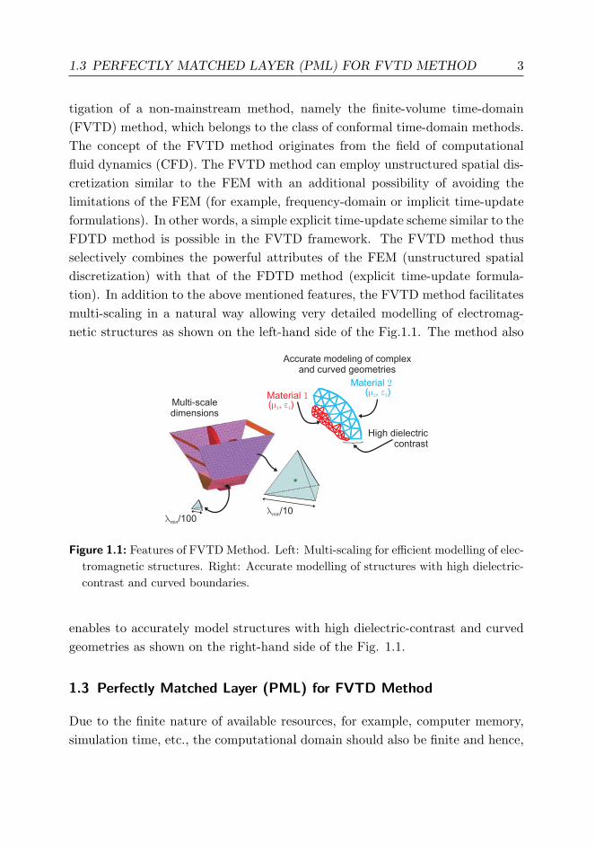
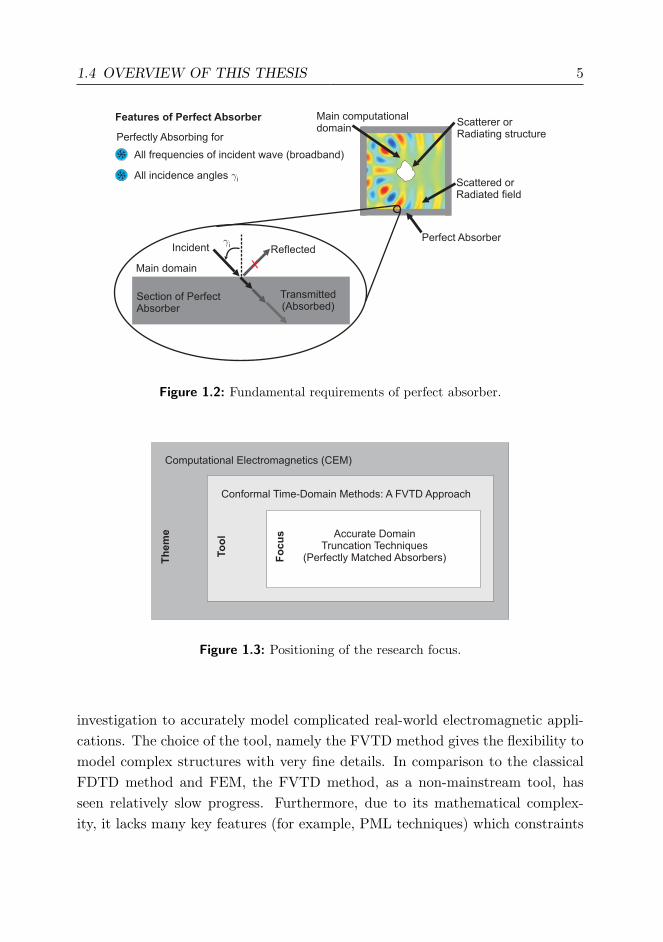
the numerical methods require very accurate computational domain truncationtechniques. In many cases, the accuracy of these truncation techniques have asignificant impact on the quality of the computed results. Therefore, the objec-tive is to develop boundary truncation techniques which can mimic an infinitecomputational space. In practice, however, there is a significant amount of un-physical reflections at the boundary of the main computational domain. Varioustechniques for domain truncation have been developed during the last couple ofdecades which are generally classified as absorbing boundary conditions (ABC)[3] demonstrating various levels of accuracy. All these ABCs perform accuratelyfor one particular case for which they were optimized. Moreover, the performanceof these ABCs depends on the order of the truncation error in terms of their Tay-lor series approximation. Higher-order ABCs also require large computationalefforts. Hence, there is a tradeoff between performance and computational effort.The idea of developing an accurate ABC which can perfectly absorb all outgoingradiations with practically negligible reflection remained a long term dream untilthe introduction of perfectly matched layer (PML) technique in 1994 by Berengerin the framework of the FDTD method. The fundamental requirements of thePML technique is to obtain theoretically perfect absorption for all frequenciesand angles of incident radiation as illustrated in Fig. 1.2. In addition, the perfor-mance of the PML is also independent of the polarisation of the incident signal.
Prior to the present research, the most well-known ABC technique for theFVTD framework was the first-order accurate Silver-Muller ABC (SM-ABC)which is optimal only for normal incident outgoing waves. In addition, becauseof the mathematical complexity of the FVTD method, there was practically noinvestigation related to PML techniques in this framework. Hence, the focusof this thesis is to investigate various PML and to develop accurate domaintruncation techniques in the FVTD framework. At the same time, this thesiscreates an organisation among various existing PML techniques based on theiranalytical formulation and theoretical relationship.
1.4 Overview of this thesis
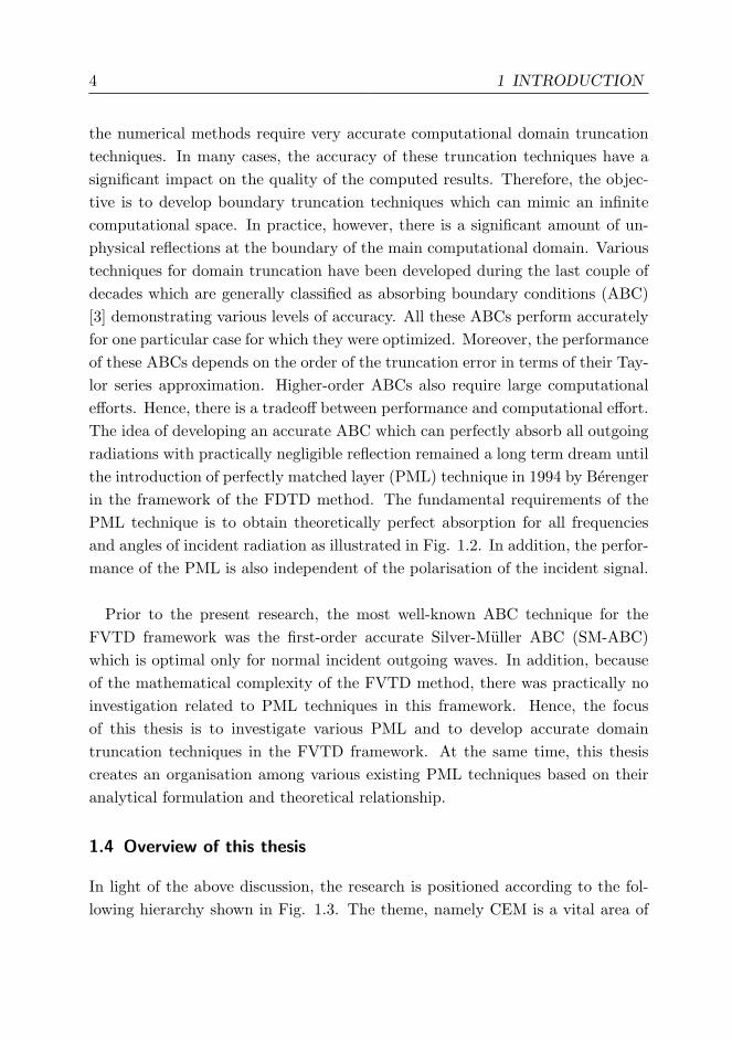
In light of the above discussion, the research is positioned according to the fol-lowing hierarchy shown in Fig. 1.3. The theme, namely CEM is a vital area of
1.4 OVERVIEW OF THIS THESIS 5
Features of Perfect Absorber
Perfectly Absorbing for
All frequencies of incident wave (broadband)
All incidence angles i
Main computationaldomain
X
Incident Reflected
Transmitted(Absorbed)
Main domain
Section of PerfectAbsorber
i
Scatterer orRadiating structure
Perfect Absorber
Scattered orRadiated field
*
*
Figure 1.2: Fundamental requirements of perfect absorber.
Computational Electromagnetics (CEM)
Conformal Time-Domain Methods: A FVTD Approach
Accurate DomainTruncation Techniques
(Perfectly Matched Absorbers)Th
em
e
To
ol
Fo
cu
s
Figure 1.3: Positioning of the research focus.
investigation to accurately model complicated real-world electromagnetic appli-cations. The choice of the tool, namely the FVTD method gives the flexibility tomodel complex structures with very fine details. In comparison to the classicalFDTD method and FEM, the FVTD method, as a non-mainstream tool, hasseen relatively slow progress. Furthermore, due to its mathematical complex-ity, it lacks many key features (for example, PML techniques) which constraints

6 1 INTRODUCTION
the full exploitation of this methodology. The driving motive of this researchis therefore to overcome these mathematical intricacies and to develop accuratedomain truncation techniques, thereby expanding the range of features for theFVTD method.
1.5 Chapter Organisation
The chapters in this thesis are organized as follows. The mathematical prelim-inaries of Maxwell equations as a system of conservation laws is introduced inChap. 2. Later the concept of conformal domain discretization is described in de-tail using the framework of the FVTD method to model the conservative Maxwellsystem. The theory of split-field PML technique is introduced in Chap. 3 anda complete characterization of the technique is presented with numerical exam-ples. The performance of the split-field PML is further compared with that ofthe existing SM-ABC. In Chap. 4, the modified Lorentz material response is usedto model finite-volume absorbers as an unsplit PML technique and a practicalapplication for waveguide truncation is discussed. The broadband performanceof the split and unsplit absorbers are investigated and the duality relationshipexisting between these two absorber models are analyzed in Chap. 5. The theoryof radial perfectly matched absorbers is introduced in Chap. 6 and the compu-tational aspects related to absorber thickness and performance are additionallyaddressed. In addition, the influence of the radius of curvature and the accu-racy of the absorber are investigated using a waveguide and a horn-antenna aspractical examples. The concept of 3D spherical perfectly matched absorber isdiscussed in Chap. 7 giving a step-by-step derivation procedure to obtain the finalfield-update equation inside the 3D PML. The issues related to implementationand the effects of focussing phenomena are investigated in detail. A complex3D problem consisting of very low-level coupling between two spiral antennasis studied to demonstrate an excellent application of the 3D PML technique incomparison with the existing SM-ABC technique.

2 Conservation Laws and Conformal Time-Domain
Modelling
Abstract — Like many natural phenomena, the time and space varying behaviour of electric
and magnetic field intensities are governed by a set of partial differential equations termed
the Maxwell equations. These equations can be represented as a system of conservation
laws. In this chapter the mathematical theory of Maxwell system is developed as Hyperbolic
system of conservation laws, which is later used to develop the conformal time-domain dis-
cretization approach.
2.1 Maxwell System
The system of equations characterizing the behaviour of spatially and temporallyvarying electric and magnetic fields is given by the Maxwell equations written as
∇×E = −∂tB (2.1)
∇×H = J + ∂tD (2.2)
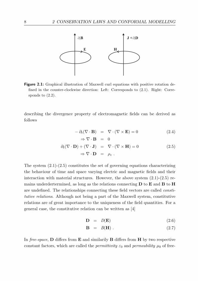
where E and H represent the electric and magnetic field intensities, respectively.The magnetic flux density and the electric displacement density are correspond-ingly denoted as B and D and the free conduction current density is given by thevector J. The differential operators ∂t and ∇× govern the rate of change withrespect to temporal variable t and rotation with respect to spatial variables x, y,and z, respectively. If positive rotation is defined in the counter-clockwise direc-tion then the above two Maxwell curl equations can be graphically illustratedas in Fig. 2.1. Apart from the above two equations, the system is additionallyconstrained by the equation of charge conservation given by
∇ · J = −∂tρv (2.3)
where ρv denotes the volume charge density. With the knowledge of equations(2.1)-(2.3) and using the vector identity ∇ · (∇×X) = 0, two further equations
7
8 2 CONSERVATION LAWS AND CONFORMAL MODELLING
Bt
E
J + Dt
H
Figure 2.1: Graphical illustration of Maxwell curl equations with positive rotation de-fined in the counter-clockwise direction: Left: Corresponds to (2.1). Right: Corre-sponds to (2.2).
describing the divergence property of electromagnetic fields can be derived asfollows
− ∂t(∇ ·B) = ∇ · (∇×E) = 0 (2.4)
⇒ ∇ ·B = 0
∂t(∇ ·D) + (∇ · J) = ∇ · (∇×H) = 0 (2.5)
⇒ ∇ ·D = ρv .
The system (2.1)-(2.5) constitutes the set of governing equations characterizingthe behaviour of time and space varying electric and magnetic fields and theirinteraction with material structures. However, the above system (2.1)-(2.5) re-mains underdertermined, as long as the relations connecting D to E and B to Hare undefined. The relationships connecting these field vectors are called consti-tutive relations. Although not being a part of the Maxwell system, constitutiverelations are of great importance to the uniqueness of the field quantities. For ageneral case, the constitutive relation can be written as [4]
D = D(E) (2.6)
B = B(H) . (2.7)
In free-space, D differs from E and similarily B differs from H by two respectiveconstant factors, which are called the permittivity ε0 and permeability µ0 of free-

2.1 MAXWELL SYSTEM 9
space written as
D = ε0E (2.8)
B = µ0H . (2.9)
However, in the case of homogeneous isotropic medium where the physical prop-erties of the medium in the neighbourhood is the same in all directions, the aboverelationship is given by
D = εE with ε = εrε0 (2.10)
B = µH with µ = µrµ0 (2.11)
where εr and µr correspond to relative permittivity and relative permeability,respectively. Correspondingly, the permittivity and permeability of the mediumare defined by ε and µ. The above relation can be rewritten in a different formwhich will be used later in Chap. 4 on material based Maxwellian absorber modelas follows
D = ε0E + P with P =
χe︷ ︸︸ ︷(εr − 1) ε0E (2.12)
B = µ0(H + M) with M =
χm︷ ︸︸ ︷(µr − 1) H (2.13)
where P and M denote polarization and magnetization, respectively. The factorsχe and χm are called the electric and magnetic susceptibilities, respectively. In thecase of anisotropic medium, where the material properties in the neighbourhooddo not stay constant in all directions, the material property strongly depends onthe directional orientation. These phenomena result in tensor permittivity ε andtensor permeability µ with directional dependence. For example, as will be seenin the later chapters, the constitutive relation (2.10) in the case of anisotropicmedium becomes
D = εE (2.14)

10 2 CONSERVATION LAWS AND CONFORMAL MODELLING
with the permittivity tensor given by
ε =
ε11 ε12 ε13
ε21 ε22 ε23
ε31 ε32 ε33
. (2.15)
In component form (2.14) is expressed as follows
Dx = ε11Ex + ε12Ey + ε13Ez (2.16)
Dy = ε21Ex + ε22Ey + ε23Ez (2.17)
Dz = ε31Ex + ε32Ey + ε33Ez . (2.18)
In an analogous manner, the constitutive relation (2.11) becomes
Bx = µ11Hx + µ12Hy + µ13Hz (2.19)
By = µ21Hx + µ22Hy + µ23Hz (2.20)
Bz = µ31Hx + µ32Hy + µ33Hz (2.21)
with permeability tensor given by
µ =
µ11 µ12 µ13
µ21 µ22 µ23
µ31 µ32 µ33
. (2.22)
The isotropic medium can be considered as a particular case of general mediumand the corresponding material equations for permittivity and permeability willhave only diagonal entries in the tensor with identical values. That is,
ε = ε[1]3×3 and µ = µ[1]3×3 (2.23)
where [1]3×3 denotes the unit 3×3 matrix. In anisotropic media, the vector pairs,namely (B, H) and (D, E) are not always parallel and the material matrices,

2.2 THEORY OF CONSERVATION LAW 11
ε and µ, are diagonalizable1 [6]. Due to this property of anisotropic media, theoff-diagonal elements in diagonal material matrices can be set to zero and hence,only the principal axes of the media contribute to the field components describedin (2.16)-(2.18) and (2.19)-(2.21) as follows [7]
Dx = ε11Ex, Dy = ε22Ey, Dz = ε33Ez (2.24)
Bx = µ11Hx, By = µ22Hy, Bz = µ33Hz . (2.25)
2.2 Theory of Conservation Law
Conservation laws are very interesting area of research encompassing a wide rangeof applications [8]. The theory of conservation laws is actively used in variousresearch studies in fluid dynamics, acoustics, and electromagnetics to model theunderlying physics. Numerical methods for solving these conservation laws areyet another area of major research [9]. The discussion presented in this sectionis a brief introduction to the theory of conservation laws which will be later usedto model electromagnetic problems.
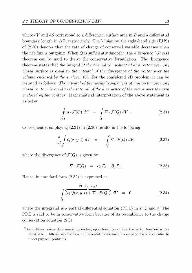
Consider a domain of interest denoted as Ω as shown in Fig. 2.2 with itsboundary denoted as ∂Ω. Let Q be the conserved scalar quantity inside thedomain Ω, which means that the integral of Q over Ω varies only due to fluxacross ∂Ω. Mathematically this can be expressed as follows
d
dt
∫Ω
Q(x, y, t) dxdy = net flux of Q across ∂Ω . (2.26)
The term net flux is obtained by integrating the flux of Q that crosses ∂Ω inthe normal direction at each point on ∂Ω. For a 2D model with no variationalong the z -axis, the flux vector is given by F(Q) = [Fx,Fy]T where Fx and Fyare the fluxes in the x and y directions, respectively. The domain Ω in this 2Dcase corresponds to the area of the entire computational domain and ∂Ω denotesthe boundary line that encloses the area Ω. For a test point on the enclosingboundary line in 2D, these two components of the flux are computed as follows:
1A square matrix [A] is called diagonalizable if it can be transformed into a diagonal matrix.
In other words, if there exists an invertible matrix [P] such that [P ]−1[A][P ] is a diagonal
matrix, then [A] is diagonalizable [5].

12 2 CONSERVATION LAWS AND CONFORMAL MODELLING
W
¶W
n
nx
ny
Figure 2.2: An example for the computational domain of interest Ω with the enclosingboundary ∂Ω shown along with the normal vector at a sample point on ∂Ω withcomponents nx and ny along the x and y axes, respectively.
1. Fx corresponds to the flux of Q in the x -direction per unit length in y, perunit time t. This means that for an interval from (x0, y0) to (x0, y0 + ∆y)over the time interval ∆t, the x component of F(Q) is given as
Fx = F(Q(x0, y0))∆y∆t . (2.27)
2. Analogously, Fy corresponds to the flux of Q in the y-direction per unitlength in x, per unit time t. That is, for an interval from (x0, y0) to (x0 +∆x, y0) over the time interval ∆t, the y component of F(Q) is given as
Fy = F(Q(x0, y0))∆x∆t . (2.28)
The x and y components of F(Q) are then projected along the normal directionat each point p on ∂Ω to get the flux (scalar) at each point as follows
n · F(Q(x(p), y(p), t)) = nxFx + nyFy . (2.29)
Thus, (2.26) can rewritten as
d
dt
∫Ω
Q(x, y, t) dV = −∮∂Ω
n · F(Q) dS (2.30)
2.2 THEORY OF CONSERVATION LAW 13
where dV and dS correspond to a differential surface area in Ω and a differentialboundary length in ∆Ω, respectively. The ’-’ sign on the right-hand side (RHS)of (2.30) denotes that the rate of change of conserved variable decreases whenthe net flux is outgoing. When Q is sufficiently smooth2, the divergence (Gauss)theorem can be used to derive the conservative formulation. The divergencetheorem states that the integral of the normal component of any vector over anyclosed surface is equal to the integral of the divergence of the vector over thevolume enclosed by the surface [10]. For the considered 2D problem, it can berestated as follows: The integral of the normal component of any vector over anyclosed contour is equal to the integral of the divergence of the vector over the areaenclosed by the contour. Mathematical interpretation of the above statement isas below ∮
∂Ω
n · F(Q) dS =∫Ω
∇ · F(Q) dV . (2.31)
Consequently, employing (2.31) in (2.30) results in the following
d
dt
∫Ω
Q(x, y, t) dV = −∫Ω
∇ · F(Q) dV, (2.32)
where the divergence of F(Q) is given by
∇ · F(Q) = ∂xFx + ∂yFy. (2.33)
Hence, in standard form (2.32) is expressed as
∫Ω
PDE in x,y,t︷ ︸︸ ︷(∂tQ(x, y, t) +∇ · F(Q)) dV = 0 (2.34)
where the integrand is a partial differential equation (PDE) in x, y, and t. ThePDE is said to be in conservative form because of its resemblence to the chargeconservation equation (2.3).
2Smoothness here is determined depending upon how many times the vector function is dif-
ferentiable. Differentiability is a fundamental requirement to employ discrete calculus to
model physical problems.

14 2 CONSERVATION LAWS AND CONFORMAL MODELLING
2.3 Maxwell System as a Conservation Law
It is assumed in the following derivation that the medium under consideration isvoid of net electric charge and current. In other words, the electric volume chargedensity ρv = 0 and the electric current density J = 0. This assumption alongwith the knowledge gained from (2.10)-(2.11) leads to the homogenous Maxwellsystem written as
µ ∂tH = −∇×E (2.35)
ε ∂tE = ∇×H (2.36)
∇ ·H = 0 (2.37)
∇ ·E = 0 . (2.38)
In (2.37)-(2.38) the RHS are identically zero corresponding to a divergence-freesystem. In CEM, the two Maxwell curl equations (2.35)-(2.36) are of practicalrelevance and the two divergence equations (2.37)-(2.38) are implicitly assumedto be satisfied. Moreover, by using the corollary of the derivations in (2.4)-(2.5),it can also be proved analytically that if all the field components are causal withinitial conditions E(t = 0, x, y) = 0 and H(t = 0, x, y, z) = 0, the abovedivergence-free conditions hold true for all later times in the continuous case3.
For simplicity, a 2D problem is considered in the following with no variationin the electromagnetic field quantities along the z -axis and propagation is in thexy-plane. For the considered 2D situation, the above system can be decoupledinto two orthogonal modes, namely the transverse electric TE and the transversemagnetic TM modes. The TE mode corresponds to the combined electromagneticfield vector given by U = [Hx, Hy, Ez]T where the superscript ‘T’ denotes matrixtranspose. The orientations of the electric and magnetic field components aredenoted as subscripts ‘x’ , ‘y’, and ‘z’. Similarly, the field components for theTM mode are given by U = [Ex, Ey, Hz]T.
3It will be later discussed that, any numerical method which is employed to mimic the above
continuous partial differential equations (PDEs) (2.35)-(2.38) using a set of difference equa-
tions modelled in the discrete computer environment should preserve this divergence-free
property. However, this property is partially violated because of the grid induced noises
which can also lead to spurious-modes in the computed solution. For most of the applica-
tions the effect of this violation is insignificant.
2.3 MAXWELL SYSTEM AS A CONSERVATION LAW 15
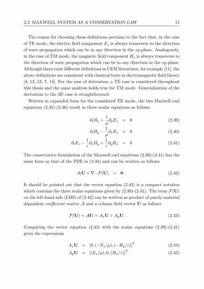
The reason for choosing these definitions pertains to the fact that, in the caseof TE mode, the electric field component Ez is always transverse to the directionof wave propagation which can be in any direction in the xy-plane. Analogously,in the case of TM mode, the magnetic field component Hz is always transverse tothe direction of wave propagation which can be in any direction in the xy-plane.Although there exist different definitions in CEM literatures, for example [11], theabove definitions are consistent with classical texts in electromagnetic field theory[4, 12, 13, 7, 14]. For the ease of derivation, a TE case is considered throughoutthis thesis and the same analysis holds true for TM mode. Generalization of thederivation to the 3D case is straightforward.
Written in expanded form for the considered TE mode, the two Maxwell curlequations (2.35)-(2.36) result in three scalar equations as follows
∂tHx +1µ∂yEz = 0 (2.39)
∂tHy −1µ∂xEz = 0 (2.40)
∂tEz −1ε∂xHy +
1ε∂yHx = 0 (2.41)
The conservative formulation of the Maxwell curl equations (2.39)-(2.41) has thesame form as that of the PDE in (2.34) and can be written as follows
∂tU +∇ · F(U) = 0 . (2.42)
It should be pointed out that the vector equation (2.42) is a compact notationwhich contains the three scalar equations given by (2.39)-(2.41). The term F(U)on the left-hand side (LHS) of (2.42) can be written as product of purely materialdependent coefficient matrix A and a column field vector U as follows
F(U) = AU = AxU +AyU . (2.43)
Comparing the vector equation (2.43) with the scalar equations (2.39)-(2.41)gives the expressions
AxU = [0, (−Ez/µ), (−Hy/ε)]T (2.44)
AyU = [(Ez/µ), 0, (Hx/ε)]T . (2.45)

16 2 CONSERVATION LAWS AND CONFORMAL MODELLING
Consequently, the x and y components of A, correspondingly denoted as Ax andAy, can be written as below
Ax =
0 0 0
0 0 − 1µ
0 −1ε 0
, Ay =
0 0 1µ
0 0 0
1ε 0 0
. (2.46)
The equation (2.42) is the starting point for deriving the conservative FVTDformulation of the discrete Maxwell system. Before deriving the discrete FVTDequations, a few words on the nature of solution of the Maxwell equations isdiscussed in the following.
2.4 Hyperbolicity and Charateristics of Maxwell System
In mathematical terms, the system (2.42) is said to be hyperbolic. The physicalmeaning of this mathematical definition is that, the system has wavelike solution[15]. This means that the material matrices Ax and Ay are diagonalizable withreal eigenvalues. Furthermore, this condition should also hold true for any linearcombination of these matrices, that is, for any arbitrary vector n, it is mandatorythat matrix A = n · A = nxAx+nyAy be diagonalizable with real eigenvalues.For the considered 2D TE the matrix A is given by
A =
0 0 ny/µ
0 0 −nx/µ
ny/ε −nx/ε 0
. (2.47)
The matrix A has three real distinct eigenvalues given by
λ1 = 0 (2.48)
λ2 =1√εµ
= +c (2.49)
λ3 =−1√εµ
= −c . (2.50)

2.4 HYPERBOLICITY AND CHARATERISTICS 17
It is worth noting that the eigenvalues are independent of the test vector n andentirely dependent on the material properties of the medium. Furthermore, theeigenvalues have the physical significance of representing the velocity of wavepropagation. In this particular case, the constant factor c corresponds to thevelocity of EM waves in the medium with permittivity ε and permeability µ.The corresponding eigenvectors give the direction of wave propagation. Theeigenvalue λ1 = 0 corresponds to a solution that propagates with zero velocitywhich represents astationary wave and hence, does not influence the propagationof information forward in time. However, as will be shown later in this chapter,this stationary wave ensures tangential continuity of electric and magnetic fieldsbetween any two dielectric media. The eigenvalues λ2 = +c and λ3 = −c areof pratical relevance as they influence the rate at which information propagatesforward in time. Hence, at each point in the computational domain, there is thena forward propagating wave with velocity +c, a reverse propagating wave withvelocity −c, and a stationary wave with velocity 0. Let the right eigenvector ofA be denoted as R and the three eigenvalues consitute a 3 × 3 diagonal matrixgiven by
Λ =
0 0 0
0 c 0
0 0 −c
. (2.51)
Then matrix A can be written in the form A = RΛR−1. The matrix A can besplit into positive and negative parts as follows
A = RΛR−1 = R(Λ+ + Λ−)R−1 = RΛ+R−1 +RΛ−R−1 = A+ + A− (2.52)
where Λ+ has only the positive eigenvalues on the diagonal with negative eigen-values replaced by zeros and vice versa for Λ−y . For the considered coefficientmatrix A the above splitting leads to the left and right coefficent matrices as

18 2 CONSERVATION LAWS AND CONFORMAL MODELLING
below
A+ =12
n2yc −nxnyc ny/µ
−nxnyc n2xc −nx/µ
ny/ε −nx/ε (n2x + n2
y)c
and (2.53)
A− =12
−n2yc nxnyc ny/µ
nxnyc −n2xc −nx/µ
ny/ε −nx/ε −(n2x + n2
y)c
. (2.54)
By comparing (2.53) and (2.54), relation between A+ and A− is obtained as
A−(n, ε, µ) = −A+(−n, ε, µ) . (2.55)
This splitting of coefficient matrix into positive (forward propagating) and neg-ative (reverse propagating) eigenvalue matrices is the main feature of the flux-splitting algorithm which will be used later in this chapter in the developmentof the MUSCL based FVTD method.
2.5 Need for Conformal Time-Domain Methods
With the advancement in computer technology and development in sophisticatedalgorithms, the level of complexity that can be accurately handled through sim-ulation also increased. To precisely model all the minute features in structureswith complex curved geometries, flexibility in spatial discretization becomes ahighly desirable attribute for computational methods. When modelling curvedor inclined structures, the standard Cartesian-grid-based FDTD method suffersfrom stair-casing errors originating from non-conforming mesh arrangements atthe curved or inclined boundaries. In practical applications, these stair-casingerrors can be minimized by reducing the size of spatial samples at the cost ofincreased computational efforts. Several research efforts are continuously made

2.5 NEED FOR CONFORMAL TIME-DOMAIN METHODS 19
to extend the standard FDTD method to model conformal geometries [16, 17].State-of-the-art solvers employing methods like transmission line matrix (TLM)method, finite integration technique (FIT) and conformal FDTD method, amongothers provide special ways to handle boundary cells which can avoid or reducestair-casing errors.
Furthermore, for layered structures with high dielectric contrast, the wavepropagation velocities vary substantially between high permittivity and low per-mittivity layers. When using the standard FDTD method for this kind of prob-lems, it becomes a challenging task to accurately resolve the difference in velocitybecause of the uniform spatial sampling.
The aforementioned shortcomings of Cartesian-grid-based methods can also beavoided by using an unstructured spatial sampling approach. Unstructured-grid-based methods adapt naturally to the curved or slanted boundaries and hence,there is no need of special treatment at the boundary cells. Finite-element-basedmethods are classical example for this kind of approach. However, the classi-cal FEM is mainly used in its frequency-domain formulation because the time-domain counterpart leads to implicit time-discretization. Generally, methodsemploying implicit time discretization are computationally heavier than explicittime-stepping methods because the former methods involve global matrix inver-sion at each time step. The speed of matrix inversion operation depends highlyon the sparseness of the matrix and the related computational effort grows ina non-linear manner constraining the size of problems that can be solved withgiven computational resources.
Hence, the objective is to capitalize on methods which can employ unstructuredspatial discretization similar to that of FEM and at the same time have a simpleexplicit time-update algorithm like classical FDTD method. This blending of thedesirable features of the FDTD method and FEM is naturally available in certainclasses of conformal time-domain methods. The FVTD method is one of the mostfundamental and simple conformal time-domain methods. The FVTD methodthat is used as the basic tool in this thesis stems from the area of CFD [18, 19, 20,21]. Like many conformal time-domain methods, the FVTD method selectivelycombines the powerful attributes of an unstructured spatial discretization withthat of a simple explicit time-update formulation. In the following, the theoryof FVTD method is discussed in detail.
20 2 CONSERVATION LAWS AND CONFORMAL MODELLING
2.6 A FVTD Approach
A 2D FVTD algorithm in an unstructured triangular grid is described in thissection. In order to develop the complete FVTD model for the Maxwell system,a few terminologies are defined.
2.6.1 Finite Volume: Definitions
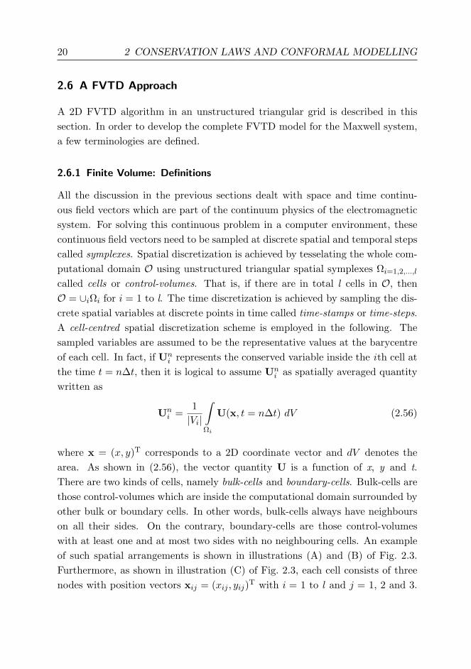
All the discussion in the previous sections dealt with space and time continu-ous field vectors which are part of the continuum physics of the electromagneticsystem. For solving this continuous problem in a computer environment, thesecontinuous field vectors need to be sampled at discrete spatial and temporal stepscalled symplexes. Spatial discretization is achieved by tesselating the whole com-putational domain O using unstructured triangular spatial symplexes Ωi=1,2,...,l
called cells or control-volumes. That is, if there are in total l cells in O, thenO = ∪iΩi for i = 1 to l. The time discretization is achieved by sampling the dis-crete spatial variables at discrete points in time called time-stamps or time-steps.A cell-centred spatial discretization scheme is employed in the following. Thesampled variables are assumed to be the representative values at the barycentreof each cell. In fact, if Un
i represents the conserved variable inside the ith cell atthe time t = n∆t, then it is logical to assume Un
i as spatially averaged quantitywritten as
Uni =
1|Vi|
∫Ωi
U(x, t = n∆t) dV (2.56)
where x = (x, y)T corresponds to a 2D coordinate vector and dV denotes thearea. As shown in (2.56), the vector quantity U is a function of x, y and t.There are two kinds of cells, namely bulk-cells and boundary-cells. Bulk-cells arethose control-volumes which are inside the computational domain surrounded byother bulk or boundary cells. In other words, bulk-cells always have neighbourson all their sides. On the contrary, boundary-cells are those control-volumeswith at least one and at most two sides with no neighbouring cells. An exampleof such spatial arrangements is shown in illustrations (A) and (B) of Fig. 2.3.Furthermore, as shown in illustration (C) of Fig. 2.3, each cell consists of threenodes with position vectors xij = (xij , yij)T with i = 1 to l and j = 1, 2 and 3.
2.6 A FVTD APPROACH 21
BulkTriangle Boundary
Triangle
BoundaryEdge
(A) (B)
(C)
ni2
xi2
ei2
ni3
xi3ei3
ni1
xi1
ei1
Figure 2.3: Geometrical aspects of an unstructured triangular spatial discretization.
Let ei1, ei2 and ei3 denote the three edges of the ith cell and analogously, ni1,ni2 and ni3 denote the three associated normal vectors of the ith cell. If |eij |denotes the length of edge eij then, a direct calculation leads to the followingexpressions for the outward-pointing unit normal vectors of ith cell [22]
ni1 =
(yi2−yi1)|ei1|
−(xi2−xi1)|ei1|
, ni2 =
(yi3−yi2)|ei2|
−(xi3−xi2)|ei2|
, ni3 =
−(yi3−yi1)|ei3|
(xi3−xi1)|ei3|
. (2.57)
Each ith cell has a measure element |Vi| corresponding to the area of the ith cellin 2D and which is expressed as
Vi = |Vi| = det
1 1 1
xi1 xi2 xi3
yi1 yi2 yi3
. (2.58)

22 2 CONSERVATION LAWS AND CONFORMAL MODELLING
2.6.2 FVTD Formulation of the Maxwell System
The FVTD formulation of Maxwell system written in the conservative form (2.42)starts with spatial integration of (2.42) inside each ith control-volume (triangle)and results in the expression similar to (2.32) as
d
dt
∫Ω
U(x, y, t) dV = −∫Ω
∇ · F(U) dV . (2.59)
Using the divergence theorem (2.31) in (2.59) the space and time continuousFVTD formulation of the Maxwell system can be expressed as
d
dt
∫Ω
U(x, y, t) dV = −∮∂Ω
n · F(U) dS . (2.60)
The term n · F(U) corresponds to the flux through the edges of a cell and hasthe following form
n · F(Uk) = n · AUk = AUk =
1µn×Ek
−1εn×Hk
(2.61)
where superscript k indicates that the electric and magnetic field values usedin the flux function are those computed values on the kth face of a cell. Forthe considered 2D TE model Ek = [0, 0, Ekz ]T and Hk = [Hk
x , Hky , 0]T. For a
triangular spatial discretization, each kth face has length |Sk| with min(k) = 1and max(k) = f = 3 and the surface area Vi is defined according to the measureelement described in (2.58). Hence, using (2.56) in (2.60) and discretizing theRHS of (2.60) using the triangular spatial discretization, the semi-discrete versionof the FVTD formulation is given by
∂tUi = − 1Vi
f∑k=1
nk · F(Uk)Sk (2.62)
= − 1Vi
f∑k=1
nk · AUkSk
It should be noted that (2.62) is discrete in space and continuous in time. Thetime discretization can be carried out in different ways. One approach it is to
2.6 A FVTD APPROACH 23
sample both the electric and magnetic field components at the same point intime. This approach leads to the collocated time-sampling scheme which canbe implemented using various time-stepping algorithms. One of the simplesttime discretization strategies is the Euler time-stepping scheme. This approachis first-order accurate in the time-sampling interval ∆t and can be written asfollows
Un+1i = Un
i −∆tVi
f∑k=1
nk · F(Uk)Sk . (2.63)
By substituting A = n·A defined in (2.47), the expression (2.63) can be rewrittenas follows
Un+1i = Un
i −∆tVi
f∑k=1
AUkSk (2.64)
= Uni −
∆tVi
f∑k=1
1µn×Ek
−1εn×Hk
Sk .It is worth mentioning that the material parameters ε and µ present in theMaxwell system (2.35)-(2.36) are contained in the definition of A (2.47). Theexpression (2.64), thus, gives the system for updating the conserved variable Ui
inside each ith cell. There are different ways to proceed from this point. Theapproach used in this thesis employs the MUSCL algorithm based on the solutionof the Riemann problem4 which will be discussed in the following.
2.6.3 Riemann Problem and Superposition of Waves
Consider an interface between two adjacent cells, namely cell i and cell j in aspace and time discretized Maxwell system. Let the field vectors in these adjacentcells be given by U− and U+, where superscripts ‘-’ and ‘+’ correspond to theLHS and RHS of the interface, respectively. The graphical illustration of thisarrangement is shown in Fig. 2.4. As illustrated in the Fig. 2.4, the field values
4Named after Bernhard Riemann who worked on a simple initial value problems in gas dy-
namics.

24 2 CONSERVATION LAWS AND CONFORMAL MODELLING
Cell i
Cell j
x 0= x 0>x 0<
Edge ij
Field Discontinuity
Top-view
Side-view
+
U
i
U
j
Figure 2.4: Discontinuity in field values in the adjacent cells in the computational do-main. The field vector state is denoted as U− for xn < 0 and U+ for xn > 0. TheLHS and RHS of the edge is denoted as -© and +©, respectively.
inside the cells are constant, and consequently, there exists a discontinuity atthe interface xn = 0. The subscript ‘n’ in the spatial variable xn denotes thatthe spatial coordinate of interest is along the normal direction with respect tothe edge. The reason for choosing the normal direction is due to the assumptionthat the field variation across an edge occurs only in the direction normal to theedge. The initial-value problem along with the definition of boundary conditionsis generally called as Initial Boundary Value Problems (IBVP) in the literature5.
For the given discontinuous field values across the interface, the procedureto obtain a unique solution at the interface is not straightforward. In order tofind a unique solution, the knowledge of characteristics of the system is veryimportant. The problem of finding an unique solution at the interface withdiscontinuous initial data using the method of characteristics is generally termedas the Riemann problem. The solution process of the Riemann problem startswith the characteristics plot of the Maxwell system given in Fig. 2.5. A briefexplanation about the characteristics plot for the Maxwell system is in orderhere. The characteristics plot is the graph of the eigenvalues of the system whichdetermines the progress of solution in space and time. It aids in computing a
5For a given initial discontinuous data and boundary condition there may exist many solutions
which might satisfy the given Maxwell system. However, there will be only one physically
meaningful solution. Physically meaningful solution additionally satisfies the entropy con-
dition which guarantees uniqueness of the solution [15, 23].

2.6 A FVTD APPROACH 25
x t -c tn
= 1 =
xn
0= 2t =
U
U
U
xn
0=
( , )txn
x cn
+
= 3t t=
x cn
+
+ txn
x cn
- t x
n
t
U
Figure 2.5: Characteristics plot for the Maxwell system: The three eigenvalues arerepresented by three grey straight lines. The field values on the LHS and RHS of theinterface in the initial state are denoted by superscripts - and +, respectively. Thecorresponding left and right intermediate states are marked with superscripts * and**, respectively.
unique solution (field vectors) at the interface between two adjacent cells withdifferent constant field values. The horizontal axis of the characteristics plotcorrespond to the normal direction at the interface and the vertical axis denotesthe time function. The information exchange (incoming and outgoing fluxes) ison either side of the interface and hence, both the positive and negative normaldirection is considered in the characteristics plot. In the case of time axis, thesolution depends on the initial data and only the time steps in the future, thatis, t > 0 is of interest. The three distinct eigenvalues of the Maxwell systemcorrespond to straight lines in the characteristics plot with inverse slopes givenby −c−, 0, and c+. The superscripts − and + correspond to the direction of wavepropagation. In fact, the eigenvalues graphed in the characteristics plot split theentire space-time region into zones. In addition to the given initial field valueswritten with superscripts − and +, there are two additional intermediate stateswhere the field values U are denoted with superscripts * and ** in the Fig. 2.5.
The solution U(xn, t) at any point (xn, t) in the space-time plane can be con-sidered as a superposition of m waves, where m = 3 is the number of independentreal eigenvalues of the Maxwell system. Furthermore, the solution U(xn, t) de-pends only on the initial data U0 = U(xn, t = 0) at m particular points xn−λpt
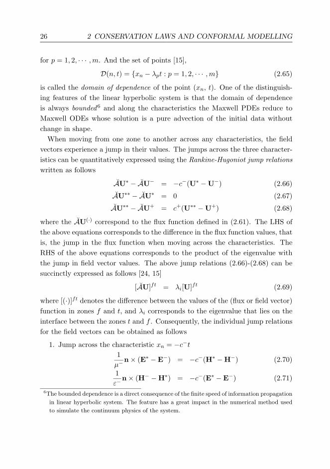
26 2 CONSERVATION LAWS AND CONFORMAL MODELLING
for p = 1, 2, · · · ,m. And the set of points [15],
D(n, t) = xn − λpt : p = 1, 2, · · · ,m (2.65)
is called the domain of dependence of the point (xn, t). One of the distinguish-ing features of the linear hyperbolic system is that the domain of dependenceis always bounded6 and along the characteristics the Maxwell PDEs reduce toMaxwell ODEs whose solution is a pure advection of the initial data withoutchange in shape.
When moving from one zone to another across any characteristics, the fieldvectors experience a jump in their values. The jumps across the three character-istics can be quantitatively expressed using the Rankine-Hugoniot jump relationswritten as follows
AU∗ − AU− = −c−(U∗ −U−) (2.66)
AU∗∗ − AU∗ = 0 (2.67)
AU∗∗ − AU+ = c+(U∗∗ −U+) (2.68)
where the AU(·) correspond to the flux function defined in (2.61). The LHS ofthe above equations corresponds to the difference in the flux function values, thatis, the jump in the flux function when moving across the characteristics. TheRHS of the above equations corresponds to the product of the eigenvalue withthe jump in field vector values. The above jump relations (2.66)-(2.68) can besuccinctly expressed as follows [24, 15]
[AU]ft = λi[U]ft (2.69)
where [(·)]ft denotes the difference between the values of the (flux or field vector)function in zones f and t, and λi corresponds to the eigenvalue that lies on theinterface between the zones t and f . Consequently, the individual jump relationsfor the field vectors can be obtained as follows
1. Jump across the characteristic xn = −c−t1µ−
n× (E∗ −E−) = −c−(H∗ −H−) (2.70)
1ε−
n× (H− −H∗) = −c−(E∗ −E−) (2.71)
6The bounded dependence is a direct consequence of the finite speed of information propagation
in linear hyperbolic system. The feature has a great impact in the numerical method used
to simulate the continuum physics of the system.

2.7 FLUX DEFINITIONS 27
2. Jump across the characteristic xn = 0
n× (E∗ −E∗∗) = 0 (2.72)
n× (H∗ −H∗∗) = 0 (2.73)
3. Jump across the characteristic xn = c+t
1µ+
n× (E+ −E∗) = c+(H+ −H∗∗) (2.74)
1ε+
n× (H∗∗ −H+) = c+(E+ −E∗∗) . (2.75)
The jump relations given by (2.70)-(2.75) translate naturally to the flux-splittingalgorithm, and in the following these relations are used to derive special fluxfunctions and interface conditions.
2.7 Flux Definitions: Special Boundary and Interface Conditions
In this section, the coefficient matrix-splitting approach (2.52)-(2.54) describedin Sect. 2.4 is shown to be equivalent to flux functions derived using the jumprelations described in the previous section. For the Maxwell system, and ingeneral for all linear hyperbolic systems, the mathematical splitting of coefficientmatrix is naturally incorporated due to real and finite information propagationvelocities [25]. Furthermore, it has a strong physical significance, for it representsthe splitting of the total flux at each edge into incoming and outgoing fluxes.The outgoing and incoming fluxes are computed using the left and right fieldapproximations at each edge in the computational domain, respectively. The leftapproximation of the field is based on the information from the left neighbourand the right approximation is based on the information from the right neighbouras illustrated in Fig. 2.6. The two velocities, namely c+ and c− correspondingto the rate of right and left wave propagation, influence the approximation ofthe field vectors on the right (U+) and left (U−) sides of an edge as shown inFig. 2.6. In order to update the field values forward in time, it is required tofind a good approximation for the field values on the edges. Later these edgefield approximations are used to compute the edge fluxes which are used in thefinal update system (2.64). In the following the jump relations derived in thelast section are used to derive special flux functions and interface conditions.
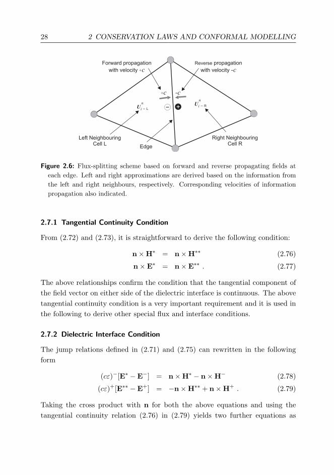
28 2 CONSERVATION LAWS AND CONFORMAL MODELLING
+
+U
i = R
n
Ui = L
n
+c -c
Edge
Left NeighbouringCell L
Right NeighbouringCell R
Forward propagation
with velocity +c
Reverse propagation
with velocity -c
Figure 2.6: Flux-splitting scheme based on forward and reverse propagating fields ateach edge. Left and right approximations are derived based on the information fromthe left and right neighbours, respectively. Corresponding velocities of informationpropagation also indicated.
2.7.1 Tangential Continuity Condition
From (2.72) and (2.73), it is straightforward to derive the following condition:
n×H∗ = n×H∗∗ (2.76)
n×E∗ = n×E∗∗ . (2.77)
The above relationships confirm the condition that the tangential component ofthe field vector on either side of the dielectric interface is continuous. The abovetangential continuity condition is a very important requirement and it is used inthe following to derive other special flux and interface conditions.
2.7.2 Dielectric Interface Condition
The jump relations defined in (2.71) and (2.75) can rewritten in the followingform
(cε)−[E∗ −E−] = n×H∗ − n×H− (2.78)
(cε)+[E∗∗ −E+] = −n×H∗∗ + n×H+ . (2.79)
Taking the cross product with n for both the above equations and using thetangential continuity relation (2.76) in (2.79) yields two further equations as
2.7 FLUX DEFINITIONS 29
follows
(cε)−[n×E∗ − n×E−] = n× n×H∗ − n× n×H− (2.80)
(cε)+[n×E∗∗ − n×E+] = −n× n×H∗ + n× n×H+ . (2.81)
Adding (2.80) and (2.81) with knowledge of the tangential continuity condition(2.77) and rearranging the terms yields the final expression for the tangential Eedge flux vector as follows
n×E∗ = n× [(cε)−E− − n×H−] + [(cε)+E+ + n×H+](cε)− + (cε)+
(2.82)
= n×Ek .
When a similar procedure is carried out using the jump relations (2.70) and(2.74), the tangential H edge flux vector is obtained as below
n×H∗ = n× [(cµ)−H− + n×E−] + [(cµ)+H+ − n×E+](cµ)− + (cµ)+
(2.83)
= n×Hk .
The numerator terms on the RHS of (2.82) and (2.83) consists of two terms. Thefirst term purely depends on the information from the LHS side of the edge andthe second term purely depends on the information from the RHS of the edge.The two terms when written in their expanded form exactly correspond to theleft and right coefficient matrices defined in (2.53) and (2.54). The expressions(2.82) and (2.83) correspond to the flux function defined across any two dielectricmedia and can be directly used in the final system (2.64) to update the E andH field vectors inside the bulk region of the computational domain.
2.7.3 Perfect Electric Conductor (PEC) Boundary Condition
Assume an edge of the cell to represent a PEC surface which has only a leftneighbour and there exists no right neighbour due to the fact that it is a boundaryedge. It is well known that for a PEC surface the tangential component of the Efield goes to zero and there is no field propagation into the PEC medium, thatis, c+ = 0. Applying these restrictions on the flux functions derived in (2.82)
30 2 CONSERVATION LAWS AND CONFORMAL MODELLING
and (2.83) results in the following flux function for the PEC boundary condtion
n×Ek = 0 (2.84)
n×Hk = n× [H− +1
(cµ)−n×E−] . (2.85)
2.7.4 Perfect Magnetic Conductor (PMC) Boundary Condition
For a boundary edge of a cell corresponding to the PMC surface the tangentialcomponent of the H field goes to zero at the interface and there is no field prop-agation into the PMC medium c+ = 0. These restrictions lead to the followingPMC flux function
n×Ek = n× [E− − 1(cε)−
n×H−] (2.86)
n×Hk = 0 . (2.87)
2.7.5 Absorbing Boundary Condition (ABC): Silver-Muller ABC
One of the widely used ABC in the FVTD modelling is the first-order accurateSilver-Muller ABC (SM-ABC). The first-order accuracy is due to the fact thatthe ABC takes only into account the information from one neighbouring cell andis accurate only for the normal incidence of the outgoing radiation. The imple-mentation of this boundary condition is straightforward because it correspondsto setting the incoming fluxes to zero and the resulting flux function have thefollowing form
n×Ek = n× [E− − 1(cε)−
n×H−] (2.88)
n×Hk = n× [H− +1
(cµ)−n×E−] . (2.89)
Because the above flux function for SM-ABC considers information from onlyone side of the edge, it corresponds to the one-way wave equation.
2.8 Spatial and Temporal Discretization Procedure
The indices of the cells on the LHS and RHS of any edge in the computationaldomain are based on the geometrical convention followed in the preprocessing
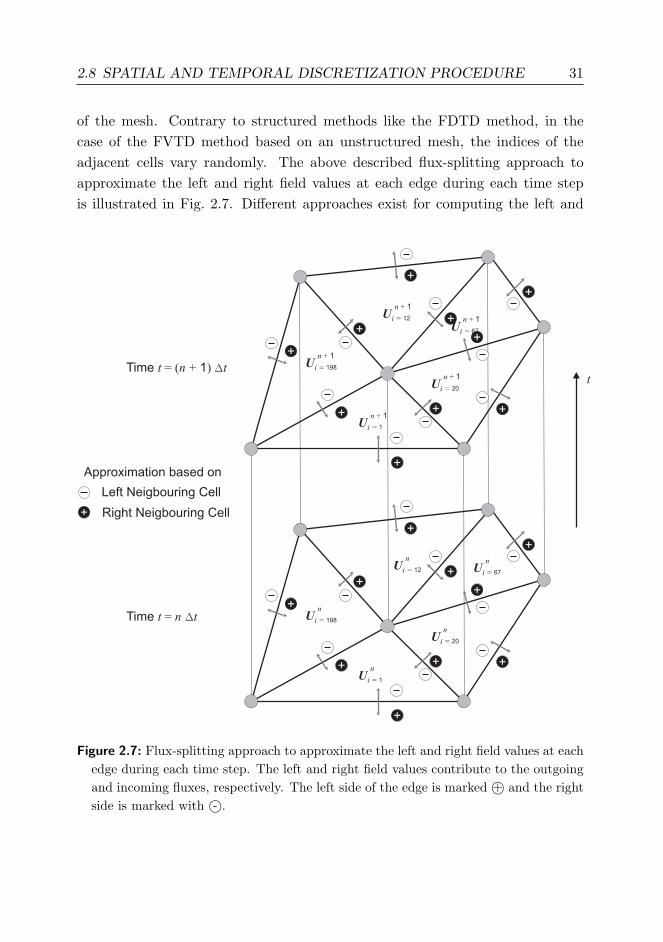
2.8 SPATIAL AND TEMPORAL DISCRETIZATION PROCEDURE 31
of the mesh. Contrary to structured methods like the FDTD method, in thecase of the FVTD method based on an unstructured mesh, the indices of theadjacent cells vary randomly. The above described flux-splitting approach toapproximate the left and right field values at each edge during each time stepis illustrated in Fig. 2.7. Different approaches exist for computing the left and
Ui = 1
n
Ui = 20
n
Ui = 198
n
Ui = 67
n
Ui = 12
n
+
++
+
+
+
+
+
+ +
Ui = 1
Ui = 20
Ui = 198
n + 1
Ui = 12
n + 1
Ui = 67
n + 1
n + 1
n + 1
+
++
+
+
+
+
+
+ +
+
Left Neigbouring Cell
Right Neigbouring Cell
Approximation based on
Time t n t= ( + )1 t
Time t n t=
Figure 2.7: Flux-splitting approach to approximate the left and right field values at eachedge during each time step. The left and right field values contribute to the outgoingand incoming fluxes, respectively. The left side of the edge is marked +© and the rightside is marked with -©.
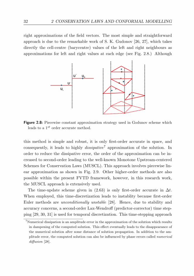
32 2 CONSERVATION LAWS AND CONFORMAL MODELLING
right approximations of the field vectors. The most simple and straightforwardapproach is due to the remarkable work of S. K. Gudonov [26, 27], which takesdirectly the cell-centre (barycentre) values of the left and right neighbours asapproximations for left and right values at each edge (see Fig. 2.8.) Although
-
+
+
+
--U
U
UL
UR
Figure 2.8: Piecewise constant approximation strategy used in Godunov scheme whichleads to a 1st order accurate method.
this method is simple and robust, it is only first-order accurate in space, andconsequently, it leads to highly dissipative7 approximation of the solution. Inorder to reduce the dissipative error, the order of the approximation can be in-creased to second-order leading to the well-known Monotone Upstream-centeredSchemes for Conservation Laws (MUSCL). This approach involves piecewise lin-ear approximation as shown in Fig. 2.9. Other higher-order methods are alsopossible within the present FVTD framework, however, in this research work,the MUSCL approach is extensively used.
The time-update scheme given in (2.63) is only first-order accurate in ∆t.When employed, this time-discretization leads to instablity because first-orderEuler methods are unconditionally unstable [28]. Hence, due to stability andaccuracy concerns, a second-order Lax-Wendroff (predictor-corrector) time step-ping [29, 30, 31] is used for temporal discretization. This time-stepping approach
7Numerical dissipation is an amplitude error in the approximation of the solution which results
in dampening of the computed solution. This effect eventually leads to the disappearance of
the numerical solution after some distance of solution propagation. In addition to the am-
plitude error, the computed solution can also be influenced by phase errors called numerical
diffusion [28].
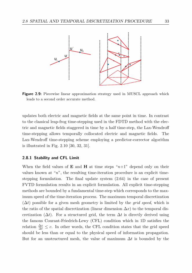
2.8 SPATIAL AND TEMPORAL DISCRETIZATION PROCEDURE 33
-
+
+
+-
-U
U
UL
UR
Figure 2.9: Piecewise linear approximation strategy used in MUSCL approach whichleads to a second order accurate method.
updates both electric and magnetic fields at the same point in time. In contrastto the classical leap-frog time-stepping used in the FDTD method with the elec-tric and magnetic fields staggered in time by a half time-step, the Lax-Wendrofftime-stepping allows temporally collocated electric and magnetic fields. TheLax-Wendroff time-stepping scheme employing a predictor-corrector algorithmis illustrated in Fig. 2.10 [30, 32, 31].
2.8.1 Stability and CFL Limit
When the field values of E and H at time steps “n+1” depend only on theirvalues known at “n”, the resulting time-iteration procedure is an explicit time-stepping formulation. The final update system (2.64) in the case of presentFVTD formulation results in an explicit formulation. All explicit time-steppingmethods are bounded by a fundamental time-step which corresponds to the max-imum speed of the time-iteration process. The maximum temporal discretization(∆t) possible for a given mesh geometry is limited by the grid speed, which isthe ratio of the spatial discretization (linear dimension ∆x) to the temporal dis-cretization (∆t). For a structured grid, the term ∆t is directly derived usingthe famous Courant-Friedrich-Lewy (CFL) condition which in 1D satisfies therelation ∆x
∆t ≤ c. In other words, the CFL condition states that the grid speedshould be less than or equal to the physical speed of information propagation.But for an unstructured mesh, the value of maximum ∆t is bounded by the

34 2 CONSERVATION LAWS AND CONFORMAL MODELLING
n
n - ½
n - 1
n + ½
n + 1
(E Hn - 1
,n - 1
)
(E Hn -
,n - ½
)½
(E Hn
,n
)
(E Hn +
,½ ½n +
)
(E Hn + 1
,n + 1
)
Time-steps Field values
Predictorsteps
Correctorsteps
Figure 2.10: Second-order accurate Lax-Wendroff scheme using a predictor and correctorscheme. The time-step for the predictor step is half that of standard Euler scheme(2.63). The corrector time-step is equal to that of standard Euler scheme.
geometry of the smallest (worst) cell in the entire computational domain. Thisfundamental limitation on the explicit formulation might become a huge bottle-neck in large models with very fine details. To battle this basic limitation on thetime-steps, a geometry-matched local-time-stepping procedure was developed in[33] to enhance the computational speed. This approach uses local geometricalinformation to separate the cells into different sub-domains. The time-updateis then carried out with different ∆t at different sample points based on thesub-domain separation.
In the following chapters, the concepts developed in this chapter are extensivelyused to develop accurate domain truncation techniques. The theoretical aspectsdiscussed so far form the basic building blocks of the advanced concepts discussedin the later chapters.
3 Split-Field Based Finite-Volume Absorber Model
Abstract — In this chapter, the perfectly matched layer model introduced by Berenger (B-
PML) using the field-splitting technique is extended for a cell-centred finite-volume time-
domain (FVTD) method. A step-by-step procedure for the performance characterization of
the B-PML is presented for both structured and unstructured finite-volume meshes. The
B-PML is compared with the standard first-order Silver-Muller absorbing boundary condition
(ABC) for practical applications. It is found that the B-PML for unstructured grid achieves
a reflection coefficient lower than −40 dB for incident angles up to 45 degrees and outper-
forms the Silver-Muller ABC by 15 to 20 dB. Furthermore, hybrid domain truncations which
employs Silver-Muller ABC in conjunction with the B-PML is studied. For certain appli-
cations, this hybrid technique provides a substitute for standard perfect electric conductor
(PEC) based truncation without extra computational effort. Strategies to adapt SM-ABC
for truncating the PML and the broadband performance analysis of the B-PML models are
explored with supporting numerical results.
3.1 Introduction
A cell-centred finite-volume time-domain (FVTD) modelling of perfectly matchedlayer introduced by Berenger (B-PML) is investigated in this chapter. A step-by-step characterization procedure for studying the performance of the B-PMLis presented. Ever since its introduction in the seminal paper [34], the PMLtechnique has matured and has been applied to a variety of simulation problemsmainly in conjunction with the finite-difference time-domain (FDTD) technique[35, 36, 37, 38]. More recently work has been reported where the PML is also usedfor other numerical techniques such as the finite-element time-domain (FETD)formulation [39, 40]. In [41], a vertex-centred FVTD model (variational ap-proach) of the PML was reported for scattering problems, but the performanceof the PML was not characterized based on its control parameters. The presentchapter extends the PML concept to the cell-centred FVTD approach and sys-
35

36 3 SPLIT-FIELD BASED FINITE-VOLUME ABSORBER MODEL
tematically characterizes its performance using both structured and unstructuredfinite-volume meshes. Furthermore, based on reflection coefficient computation,the suitability of the B-PML for practical problems is addressed. The perfor-mance of B-PML is compared with standard first-order Silver-Muller absorbingboundary condition (SM-ABC). As a practical example, the reflection coefficientis computed for the truncation of a parallel-plate waveguide using B-PML andis compared with that of SM-ABC.
For certain applications, the classical ABCs like Enguist-Majda ABC [42],Higdon ABC [43], Trefethen-Halpern ABC [44], Bayliss-Gunzburger-Turkel ABC[45], etc., can be employed as the truncating boundary condition for PML insteadof the classical PEC truncation. Combining PML and ABC has been previouslyinvestigated in [46, 47] in the framework of the finite-element frequency-domain(FEFD) method for scattering applications. These analyses were based on thestretched-coordinate approach for constructing a perfectly matched absorbinglayer as discussed in [35]. This chapter further explores the improvement in theperformance of the standard B-PML when employed in conjunction with theSM-ABC as a hybrid B-PML. The choice of SM-ABC for this hybrid domaintruncation is justified by the simple implementation that requires no additionalcomputational cost in the present FVTD framework. The implementation issuesrelated to the adaptation of SM-ABC to the split-field PML are discussed with anadditional emphasis on computational aspects of the approach. The broadbandperformance of the hybrid B-PML using a pulsed-FVTD source excitation isdemonstrated and compared to that of the pure domain truncation techniques,namely B-PML with PEC and pure SM-ABC.
3.2 FVTD Formulation of B-PML
The cell-centred FVTD formulation of PML is based on modifying the updateequations (2.35) and (2.35) with lossy material property in order to absorb theincident EM wave as
− µ ∂tH = ∇×E− σMH (3.1)
ε ∂tE = ∇×H− σEE (3.2)
where σE and σM refer to electric and magnetic conductivities, respectively. Ifa plane wave traveling across a free space-PML interface satisfies the perfect

3.2 FVTD–B-PML MODEL 37
matching condition σE/ε = σM/µ ≡ σ inside the PML domain then, thisensures reflectionless transmission of the plane wave into the PML [34].
The solutions of the PDEs defining the Maxwell system in TE form havethree unknowns, namely the transverse electric field component in z -direction(Ez), and two magnetic field components in x and y directions given by Hx
and Hy, respectively. The field vector for this analysis is represented as U =[Hx, Hy, Ez]T . As proposed in [34], the total electric field Ez is defined as a sumof two unphysical electric field components, namely Ezx and Ezy, that is, Ez =Ezx + Ezy. The lossy term σ is also correspondingly split into two componentsdenoted as σx and σy. This leads to the split field equations (including losses)introduced as
µ ∂tHx = −∂y(Ezx + Ezy)− σyHx (3.3)
µ ∂tHy = ∂x(Ezx + Ezy)− σxHy (3.4)
ε ∂tEzx = ∂xHy − σxEzx (3.5)
ε ∂tEzy = −∂yHx − σyEzy . (3.6)
3.2.1 Definition of Flux Functions
The field update equations of the finite-volume formulation are interconnected bythe flux function which facilitates communication between adjacent cells at therespective cell boundaries. The information is transmitted with a finite velocity,which is equal to the velocity of electromagnetic (EM) waves in the computationalmedium O. The whole computational domain O is considered as a union ofthe main domain (Omain) and the truncated PML domain (Opml), that is, O ≡Omain∪Opml. For simplicity, free space is assumed for Omain and a lossy mediumwith matched impedance in Opml. The FVTD method demands the preservationof the hyperbolic nature of Maxwell’s equation system in order to use the fluxsplitting technique [31]. To achieve this, the system (3.3)-(3.6) is modified usingthe relation Ezx = Ez − Ezy [41] as
µ ∂tHx = −∂yEz − σyHx (3.7)
µ ∂tHy = ∂xEz − σxHy (3.8)
ε ∂tEz = ∂xHy − ∂yHx − σxEz − (σy − σx)Ezy (3.9)
ε ∂tEzy = −∂yHx − σyEzy . (3.10)

38 3 SPLIT-FIELD BASED FINITE-VOLUME ABSORBER MODEL
Integrating the system (3.7)-(3.10) over each cell in the computational domainwith area A and perimeter S, and employing the divergence theorem results inthe conservative form as below
µ ∂t
∫A
Hx dA = −∫S
n · FHx dS
−∫A
σyHx dA (3.11)
µ ∂t
∫A
Hy dA = −∫S
n · FHy dS
−∫A
σxHy dA (3.12)
ε ∂t
∫A
Ez dA = −∫S
n · FEz dS
−∫A
(σxEz − (σy − σx)Ezy)dA (3.13)
ε ∂t
∫A
EzydA = −∫S
n · FEzy dS
−∫A
σyEzy dA . (3.14)
The resulting system (3.11)-(3.14) still remains non-hyperbolic due to the un-physical nature of field splitting introduced in the PML. Nevertheless, imposingthe initial constraint that when t = 0, the field Ezy = 0 inside Opml ensuresthat the resulting system behaves like a hyperbolic system. The term n · F in(3.11)-(3.14) is the flux function in the FVTD formulation defined in (2.61). Forsimplicity, in the following F(.) · n is denoted as Ψ(.).
Except for the lossy terms (σx and σy), (3.11)-(3.13) refers to the original TEzformulation of Maxwell equations. Hence the standard FVTD formulation isused to update (3.11)-(3.13) [48, 31]. But there is no direct way to compute theflux term in (3.14). The unphysical field Ezy is forced to be zero inside Omainand it is updated only inside Opml. In the following, the flux function for (3.14),that is, ΨEzy is modelled using the Rankine-Hugoniot jump relations defined in(2.66)-(2.68).
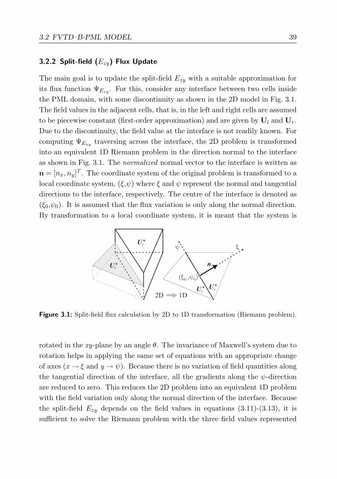
3.2 FVTD–B-PML MODEL 39
3.2.2 Split-field (Ezy) Flux Update
The main goal is to update the split-field Ezy with a suitable approximation forits flux function ΨEzy . For this, consider any interface between two cells insidethe PML domain, with some discontinuity as shown in the 2D model in Fig. 3.1.The field values in the adjacent cells, that is, in the left and right cells are assumedto be piecewise constant (first-order approximation) and are given by Ul and Ur.Due to the discontinuity, the field value at the interface is not readily known. Forcomputing ΨEzy traversing across the interface, the 2D problem is transformedinto an equivalent 1D Riemann problem in the direction normal to the interfaceas shown in Fig. 3.1. The normalized normal vector to the interface is written asn = [nx, ny]T . The coordinate system of the original problem is transformed to alocal coordinate system, (ξ,ψ) where ξ and ψ represent the normal and tangentialdirections to the interface, respectively. The centre of the interface is denoted as(ξ0,ψ0). It is assumed that the flux variation is only along the normal direction.By transformation to a local coordinate system, it is meant that the system is
Figure 3.1: Split-field flux calculation by 2D to 1D transformation (Riemann problem).
rotated in the xy-plane by an angle θ. The invariance of Maxwell’s system due torotation helps in applying the same set of equations with an appropriate changeof axes (x→ ξ and y→ ψ). Because there is no variation of field quantities alongthe tangential direction of the interface, all the gradients along the ψ-directionare reduced to zero. This reduces the 2D problem into an equivalent 1D problemwith the field variation only along the normal direction of the interface. Becausethe split-field Ezy depends on the field values in equations (3.11)-(3.13), it issufficient to solve the Riemann problem with the three field values represented

40 3 SPLIT-FIELD BASED FINITE-VOLUME ABSORBER MODEL
by the field vector U∗ = [Hξ, Hψ, Ez]. Hence the resulting 1D PDE is written as
∂tU∗ + ∂ξ ΨU∗ = 0 (3.15)
where Ψ represents the flux function. The additional constraints required tosolve (3.15) are given by the initial conditions at time t = 0 as
U∗(ξ, ψ, t = 0) =
U∗l , ξ < ξ0
U∗r , ξ > ξ0
(3.16)
Considering (3.7)-(3.9) and the rotational invariance of the Maxwell system fromthe global (x,y) axes to the local (ξ,ψ) axes, the flux function for (3.15) is obtainedas Ψ = [0,−Ez,−Hψ]T .
The solution to (3.15) is uniquely obtained by studying the system-characteristiccurves in the space-time plane as represented in Fig. 3.2. The characteristics cor-
Figure 3.2: Solution to 1D Riemann problem using Rankine–Hugoniot jump relation.
respond to the direction and speed of propagation of the field solutions at differentspace-time stamps. In Fig. 3.2, γl and γr represents the left and right movingcharacteristics originating from the interface centre with ξ = ξ0 (compare withFig. 3.1). The field values on the left of the interface (ξ = ξl) is given by Ul
and likewise on the right side (ξ = ξr) it is equal to Ur. The two characteris-tics (γl and γr) divide the space-time cell into four distinct regions denoted asregion 1 to region 4 in Fig. 3.2 with respective field values, namely U1 to U4.In order to solve for the split-field flux ΨEzy , the field values at ξ0 (see Fig. 3.2)

3.2 FVTD–B-PML MODEL 41
are required. From (3.10), the split-field flux function ΨEzy at the centre of theinterface (ξ0,ψ0) is derived as
ΨEzy = ny Hx0 (3.17)
where Hx0 is the x -component of the magnetic field along the centre region withξ = ξ0. To compute the field values at the centre of the interface the Rankine-Hugoniot jump condition is used. This condition states that, the difference influx across an interface with discontinuity is proportional to the difference infield values across the interface. In the mathematical sense, the above statementreads as
A · (U∗2 −U∗1) = sl(U∗2 −U∗1) (3.18)
A · (U∗4 −U∗3) = sr(U∗4 −U∗3) (3.19)
A · (U∗3 −U∗2) = s0(U∗3 −U∗2) (3.20)
where A is the Jacobian matrix of the system [31]. The constant of proportion-ality ‘sj ’ in (3.18)-(3.20) represents the propagation speed of discontinuity dueto the j -th characteristic. At any time t > tn, sj is given by
sj =ξ − ξ0
t− tn. (3.21)
It is noted that the term A · U∗ numerically corresponds to the flux functionΨU∗ . The values of sj , that is, the speed at which the characteristics propagateis directly obtained from the eigenvalues of the hyperbolic system. As discussedin Chap. 2, the system considered here has three distinct real eigenvalues corre-sponding to the characteristic propagation velocities given by sl = −c, sr = c,and s0 = 0. It is noted from the value of U∗ that, Ez is unaltered by the rotationto local coordinates and hence, it is required only to find normal and tangentialcomponents of the magnetic field values in region 2 and region 3. Subsequently,using the above discussion and solving (3.18)-(3.20), gives unique values of thefield in region 2 as
Hξ2 = Hξ1 (3.22)
Hψ2 = Hψ1 +12
(c4ε4Ez4 − c1ε1Ez1)
+12
(Hψ4 −Hψ1) (3.23)

42 3 SPLIT-FIELD BASED FINITE-VOLUME ABSORBER MODEL
where c(.) and ε(.) correspond to the velocity and permittivity components in theregion (.), respectively. Similarly in region 3 the unique field values are as follows
Hξ3 = Hξ4 (3.24)
Hψ3 = Hψ4 +12
((c4ε4Ez4 − c1ε1Ez1)
−12
(Hψ4 −Hψ1) . (3.25)
In order to obtain the field values along the centre of the interface, the symmetryof Maxwell’s system is used. This approximates the fields at the centre region ofthe interface as an average of the field values from region 2 and region 3 as givenbelow
Hξ0 = (1/2)(Hξ1 +Hξ4) (3.26)
Hψ0 =12
(Hψ1 +Hψ4) +12
(c4ε4Ez4 − c1ε1Ez1) (3.27)
where the subscript ‘0’ represents the centre region. The field values in globalcoordinates are directly obtained from (3.26)-(3.27) by appropriate rotation ofmatrix R as follows
Hξ0
Hψ0
Ez
R=⇒
Hx0
Hy0
Ez
. (3.28)
The rotation matrixR for a rotation through an angle θ in the xy-plane is writtenas
cos θ − sin θ 0
sin θ cos θ 0
0 0 1
(3.29)
where cos θ = nx and sin θ = ny with the previously defined nx and ny (normal-ized normal components of the interface). Using (3.26)-(3.27) in (6.1) gives an

3.2 FVTD–B-PML MODEL 43
expression for Hx0. This is the magnetic field which is required to compute thesplit-field flux ΨEzy in (3.17). Hence the final expression for ΨEzy is as follows
ΨEzy =ny2
(Hx1 +Hx4)−n2y
2(c4ε4Ez4 − c1ε1Ez1) (3.30)
=ny2
(Hxl +Hxr)−n2y
2(crεrEzr − clεlEzl) . (3.31)
The final expression of ΨEzy consists of flux contribution due to upwind flux-splitting which corresponds to the first term on the right-hand side in (3.31).The second term on the right-hand side in (3.31) denotes the correction fac-tor generally used in all upwind approximations. Using ΨEzy along with theother three standard flux terms the complete system (3.11)-(3.14) is updated atdifferent space-time steps with some additional boundary conditions which arediscussed in the following.
3.2.3 Model problem – Parallel-plate Waveguide
The problem used in this chapter is a simple parallel-plate wave guiding structureinfinitely long in the z -axis as shown in the Fig. 3.3. A plane wave is simulated
Figure 3.3: Model domain used for characterizing B-PML.
by forcing a sinusoidal electric and magnetic field along the boundary planereferred as source-plane in Fig. 3.3. For guiding the plane wave, PMC BC areimposed on both infinite plates inside Omain. The computational domain Omain
44 3 SPLIT-FIELD BASED FINITE-VOLUME ABSORBER MODEL
is truncated using a B-PML domain Opml which extends one wavelength in the( x)-direction (that is, dpml = 1λ, unless otherwise stated) and is perpendicular tox -axis. This thickness is chosen as an empirical trade-off between computationalcost and PML performance. For numerical simplicity and flexibility, the wholecomputational domain (that is, both Omain and Opml) is treated as a singleentity for the analysis. The split-field (Ezy) which plays no role inside Omain isforced to be zero inside Omain and its value becomes important only inside Opml.It is worth noting that the boundary conditions have to be modified in orderto take care of the split-field Ezy inside Opml which results in hybrid PMC BCdenoted as PML-PMC. To characterize the B-PML, a perfect electric conductor(PEC) boundary condition is used for truncating the B-PML (referred as PML-PEC). This provides equal reflection of the plane wave for all angles of incidenceand hence, strictly measures the B-PML performance. Furthermore, by usingPML-PEC, any additional influence of the truncating BCs (like SM-ABC) onthe B-PML is also avoided. The split-field flux ΨEzy for both PML-PMC andPML-PEC is computed using only the upwind information without correctionfactor as
ΨEzy = nyHxl . (3.32)
The tangential component of electric field (Ez) is zero for the PML-PEC BC. Thisimplies that the correction factor is also zero. For PML-PMC BC Ezl = Ezr, andhence the correction factor becomes zero according to (3.31). The performanceof the cell-centred B-PML is analyzed using the above described model. Variousnumerical experiments have been carried out and are discussed in-depth in thefollowing section.
3.3 Numerical Experiments
Numerical experiments presented in this chapter characterize the B-PML basedon different factors like conductivity profile, PML thickness, convergence etc. Thecentral idea is to compare the PML performance using its reflection coefficient(Γ) under different test conditions, that is, for different thickness, profile andspatial discretization. To achieve this goal on an unstructured mesh, the wholeanalysis of the B-PML performance becomes complicated. Hence the problem isdivided into two main streams as follows:

3.3 NUMERICAL EXPERIMENTS 45
1. In the first part of the numerical experiments an ideally structured FVTDtriangular mesh, as shown on the LHS of Fig. 3.4, is used in the PMLregion to investigate the optimal conductivity profile, thickness and spatialdiscretization. A structured grid approach is helpful to determine the bestpossible PML performance that can be achieved using the FVTD method,keeping the mesh-induced errors to the bare minimum.
2. In the second part, knowledge gained from the first set of numerical exper-iments is applied on a more general setup using highly unstructured trian-gular FVTD mesh as represented on the RHS of Fig. 3.4. Furthermore, toadd more practical value to this investigation, the reflection coefficient ofthe B-PML is computed at different angles of plane wave incidence.
Figure 3.4: Structured-type and unstructured-type triangular meshes.
The numerical reflection coefficient (Γ) is computed by subtracting the field val-ues inside the test model from that of a reference. The reference model is builtas an extended version of the test model and is truncated at a larger distancefrom the source.
3.3.1 Influence of the B-PML profile
In the discretized PML domain, the variation of the conductivity profile (σ) in-side the PML as a function of distance (x ) substantially affects its performance.If a constant profile with very high conductivity (σ0) is used then the numeri-cal reflection from the free space-PML interface substantially increases. On the
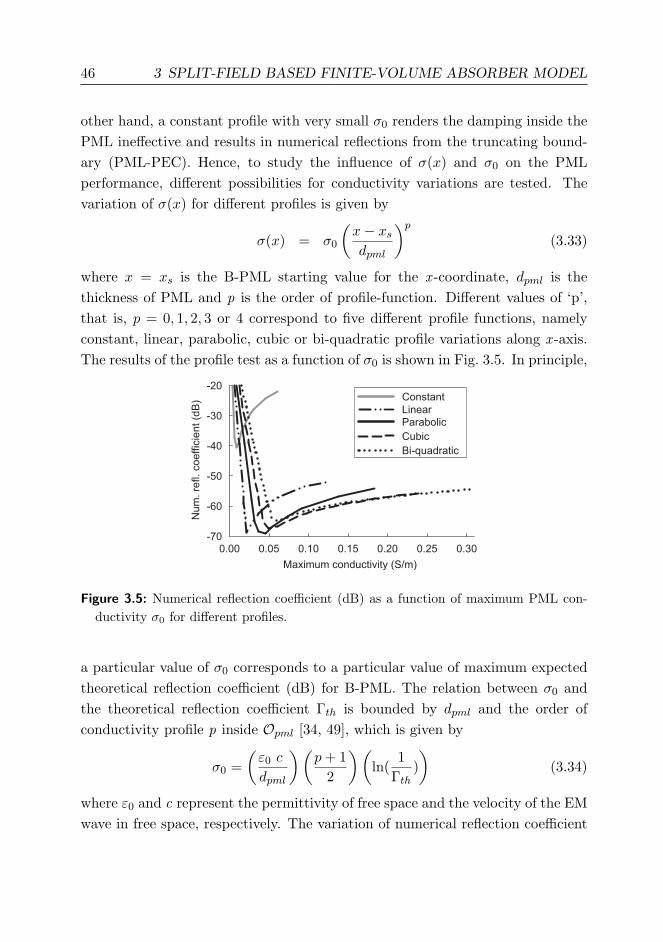
46 3 SPLIT-FIELD BASED FINITE-VOLUME ABSORBER MODEL
other hand, a constant profile with very small σ0 renders the damping inside thePML ineffective and results in numerical reflections from the truncating bound-ary (PML-PEC). Hence, to study the influence of σ(x) and σ0 on the PMLperformance, different possibilities for conductivity variations are tested. Thevariation of σ(x) for different profiles is given by
σ(x) = σ0
(x− xsdpml
)p(3.33)
where x = xs is the B-PML starting value for the x -coordinate, dpml is thethickness of PML and p is the order of profile-function. Different values of ‘p’,that is, p = 0, 1, 2, 3 or 4 correspond to five different profile functions, namelyconstant, linear, parabolic, cubic or bi-quadratic profile variations along x -axis.The results of the profile test as a function of σ0 is shown in Fig. 3.5. In principle,
Figure 3.5: Numerical reflection coefficient (dB) as a function of maximum PML con-ductivity σ0 for different profiles.
a particular value of σ0 corresponds to a particular value of maximum expectedtheoretical reflection coefficient (dB) for B-PML. The relation between σ0 andthe theoretical reflection coefficient Γth is bounded by dpml and the order ofconductivity profile p inside Opml [34, 49], which is given by
σ0 =(ε0 c
dpml
)(p+ 1
2
)(ln(
1Γth
))
(3.34)
where ε0 and c represent the permittivity of free space and the velocity of the EMwave in free space, respectively. The variation of numerical reflection coefficient

3.3 NUMERICAL EXPERIMENTS 47
as a function of theoretical reflection coefficient is shown in the Fig. 3.6.
Figure 3.6: Numerical reflection coefficient (dB) as a function of theoretical reflectioncoefficient (dB) for different profiles.
From the results shown in Fig. 3.5 and Fig. 3.6, it is clearly noticeable that aB-PML with constant profile does not yield satisfactory performance. In spite ofthe matched impedance condition between the two domains (Omain and Opml),high numerical reflection arises from discretization errors in the presence of largeconductivity steps. In other words, unlike the continuous case, the discretizedfield equations are very sensitive to sudden changes in the parameters of adjacentcells. On the other hand, a smooth and gradual increase in conductivity allowsthe impinging EM waves to encounter larger values of σ(x) only at some sufficientdepth inside the B-PML domain. This helps in attenuating the reflections dueto larger values of conductivity deep inside the B-PML using the initial dampinglayers. Among the different options the parabolic profile allows to reach the low-est reflection coefficient for a given B-PML thickness. Furthermore, the tolerancerange of a parabolic profile is larger compared to other options. In the presentsimulation, with a parabolic profile it was possible to reach a numerical reflec-tion coefficient (Γ) in the order of −70 dB for the chosen spatial discretization.Consequently, the parabolic profiling is used for the following further analysis.

48 3 SPLIT-FIELD BASED FINITE-VOLUME ABSORBER MODEL
3.3.2 Influence of B-PML thickness
Various models for optimal B-PML thickness are simulated in the range dpml =0.4λ · · · 1.0λ. The spatial discretization used corresponds to linear dimensionclose to λ/10. The results obtained are shown in Fig. 3.7. As expected, the
Figure 3.7: Numerical reflection coefficient (dB) as a function of theoretical reflectioncoefficient (dB) for different B-PML thickness (dpml). The spatial discretization isconstant (λ/10).
performance of B-PML improves as the PML thickness increases. This is mainlydue to the increase in damping distance inside the PML. The impinging EMwave undergoes initial damping on the way towards the truncating PML-PECBC and after getting reflected from PML-PEC, it is once again damped on thereturn path towards the free space-PML interface. The theoretically expectedvalues are also plotted in comparison to the performance of the discrete B-PMLmodel. The results show that for the discretization used here a PML thicknessof around 1λ is a good choice for most practical problems. This thickness is usedfor the rest of the numerical experiments.
3.3.3 Convergence Analysis of B-PML
The discrete model of the PML introduces imperfections in the perfect continuousPML. This imperfection results in a deviation of the discrete solution from theanalytical model. Hence it is instructive to test the rate of convergence for theB-PML model to understand the behaviour of the discrete B-PML models for a
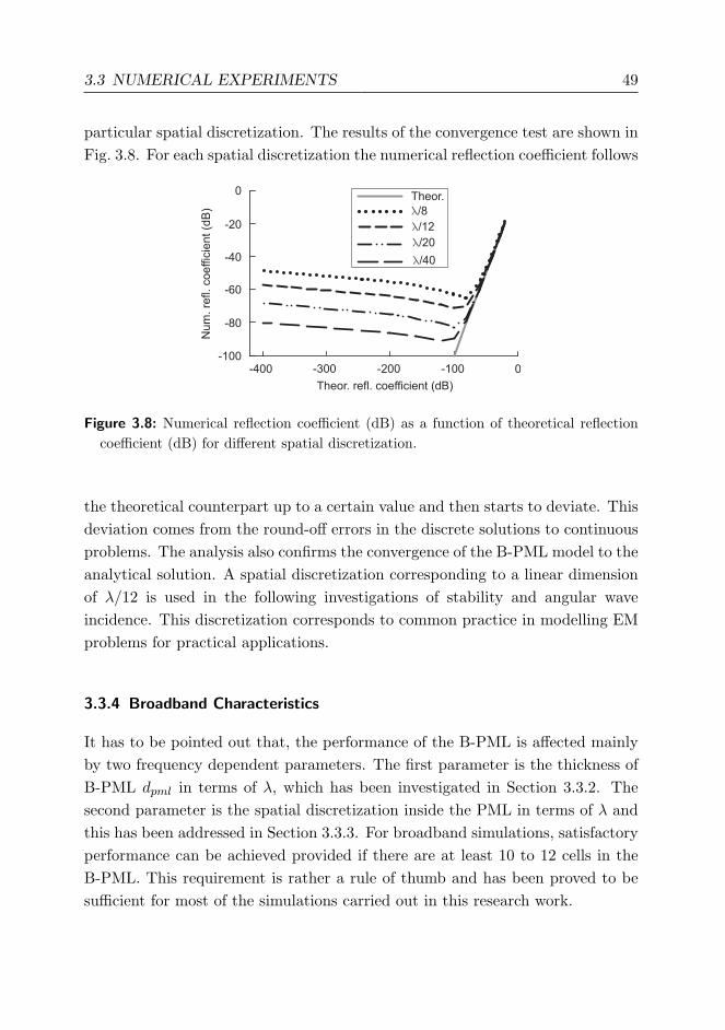
3.3 NUMERICAL EXPERIMENTS 49
particular spatial discretization. The results of the convergence test are shown inFig. 3.8. For each spatial discretization the numerical reflection coefficient follows
Figure 3.8: Numerical reflection coefficient (dB) as a function of theoretical reflectioncoefficient (dB) for different spatial discretization.
the theoretical counterpart up to a certain value and then starts to deviate. Thisdeviation comes from the round-off errors in the discrete solutions to continuousproblems. The analysis also confirms the convergence of the B-PML model to theanalytical solution. A spatial discretization corresponding to a linear dimensionof λ/12 is used in the following investigations of stability and angular waveincidence. This discretization corresponds to common practice in modelling EMproblems for practical applications.
3.3.4 Broadband Characteristics
It has to be pointed out that, the performance of the B-PML is affected mainlyby two frequency dependent parameters. The first parameter is the thickness ofB-PML dpml in terms of λ, which has been investigated in Section 3.3.2. Thesecond parameter is the spatial discretization inside the PML in terms of λ andthis has been addressed in Section 3.3.3. For broadband simulations, satisfactoryperformance can be achieved provided if there are at least 10 to 12 cells in theB-PML. This requirement is rather a rule of thumb and has been proved to besufficient for most of the simulations carried out in this research work.

50 3 SPLIT-FIELD BASED FINITE-VOLUME ABSORBER MODEL
3.3.5 Numerical Stability of B-PML Model
Most of the PML models suffer from stability problems due to an ill-posed dis-crete model. If the numerical experiment remains stable even for extremelylong-time run simulations then this indicates sufficient stability for practical ap-plications. As an experimental approach, the B-PML model is tested for long-time simulation runs (around 2500 time-periods). The result of the simulation isshown in Fig. 3.9. The energy inside the whole computational domain is boundedand this demonstrates the overall stability of the B-PML model even at the verylate time steps.
Figure 3.9: Energy inside B-PML model as a function of time period.
3.3.6 Angular Dependence of B-PML Reflection Coefficient
All the aforementioned tests performed at normal incidence provide a guidancein the selection of optimal profile, thickness, and spatial discretization for theB-PML model. But for the use in practical situations, the most relevant char-acteristic is the performance of the PML in terms of its reflection coefficient atdifferent angles of wave incidence. In addition, an unstructured mesh is used tomodel the angular response in order to represent a more general and practical sit-uation. Furthermore, for the performance comparison, the standard first-orderSilver-Muller ABC (SM-ABC) is used as a reference BC. The results for theangular wave incidence is shown in Fig. 3.10.
In theory the reference SM-ABC is accurate for normal incidence. However ina 2D simulation the computation of the gradient suffers from inaccuracies near
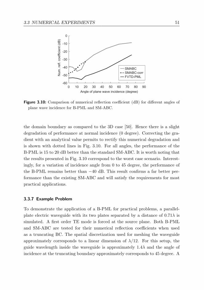
3.3 NUMERICAL EXPERIMENTS 51
Figure 3.10: Comparison of numerical reflection coefficient (dB) for different angles ofplane wave incidence for B-PML and SM-ABC.
the domain boundary as compared to the 3D case [50]. Hence there is a slightdegradation of performance at normal incidence (0 degree). Correcting the gra-dient with an analytical value permits to rectify this numerical degradation andis shown with dotted lines in Fig. 3.10. For all angles, the performance of theB-PML is 15 to 20 dB better than the standard SM-ABC. It is worth noting thatthe results presented in Fig. 3.10 correspond to the worst case scenario. Interest-ingly, for a variation of incidence angle from 0 to 45 degree, the performance ofthe B-PML remains better than −40 dB. This result confirms a far better per-formance than the existing SM-ABC and will satisfy the requirements for mostpractical applications.
3.3.7 Example Problem
To demonstrate the application of a B-PML for practical problems, a parallel-plate electric waveguide with its two plates separated by a distance of 0.71λ issimulated. A first order TE mode is forced at the source plane. Both B-PMLand SM-ABC are tested for their numerical reflection coefficients when usedas a truncating BC. The spatial discretization used for meshing the waveguideapproximately corresponds to a linear dimension of λ/12. For this setup, theguide wavelength inside the waveguide is approximately 1.4λ and the angle ofincidence at the truncating boundary approximately corresponds to 45 degree. A

52 3 SPLIT-FIELD BASED FINITE-VOLUME ABSORBER MODEL
numerical reflection coefficient of −16 dB is obtained using SM-ABC. But whenthe B-PML is employed, the numerical reflection coefficient for the same setupis as low as −42 dB. This clearly proves the excellent performance of the B-PMLover SM-ABC.
3.4 Hybrid Domain Truncation: B-PML + SM-ABC
3.4.1 Internal and Boundary Interface Treatments
ABCs, as a general category of computational domain truncation techniques, arelocal in their mathematical formulations [44, 42, 43, 45]. They are generally op-timized for a particular angle of incidence and their performance depends on thecharacteristics of the local variation in the field quantities along the truncatingboundary. As discussed in Sec. 2.7.5, the widely used SM-ABC is optimized fornormal incident of outgoing radiation. In the following, the performance andaccuracy of the SM-ABC is investigated for the FVTD simulation. With thisobjective, a model 2D problem involving a parallel-plate waveguide as shown inthe Fig. 3.11 is chosen. As depicted in the illustration, enforcing a PMC BC
Figure 3.11: Different boundary types illustrated using a parallel-plate waveguide ex-ample.
along the walls of the parallel-plate guarantees plane wave propagation alongthe waveguide for the assumed TE formulation. A plane wave hard-source isforced along the top-boundary of the parallel-plate waveguide as shown in the

3.4 HYBRID DOMAIN TRUNCATION: B-PML + SM-ABC 53
Fig. 3.11 and the bottom-boundary is truncated using the SM-ABC. The wholecomputational-domain is discretized using conformal triangular cells and the flux-function is computed across each interface present in the domain. Depending onthe position in the computational domain, each interface is categorized as inter-nal or boundary interface as shown in the Fig. 3.11. For each internal interface,there exist always two neighbouring cells which share the common boundary andthe flux traversing across each internal interface is decomposed into outgoing andincoming fluxes, that is, left-to-right and right-to-left moving fluxes, respectively.The computation of the numerical outgoing or incoming fluxes is dependent onspatial extrapolation of the field values from the corresponding barycentre valuesin cells i and j. In the present study, a second-order accurate MUSCL algorithm[51, 31] is employed to compute the field values at the left and right side of theinterface. The treatment of the PMC BC is based on the definition of PMC fluxfunction defined in Sec. 2.7.4. For the SM-ABC boundary treatment, both thetangential electric and magnetic field components contribute to the outgoing fluxsatisfying the constraint along the boundary given by
Y nk ×EL + nk × (nk ×HL) = 0 (3.35)
where Y =√
(ε/µ) is the wave-admittance in the left neighbouring cell of theSM-ABC interface, nk corresponds to the normal vector along the boundaryinterface. The above contraint results in the SM-ABC flux function defined inSec. 2.7.5. Theoretically, by ensuring the above relation (3.35) along the SM-ABCinterface, the incident EM wave which comes normal to the interface is completelyabsorbed. However, outgoing radiations meeting the SM-ABC interface at off-normal angles is only partially absorbed, and a part of it is reflected back intothe main computational-domain.
3.4.2 PML Boundary Condition
Instead of choosing a boundary condition which depends on the local character-istics of the incoming wave, the PML technique can be employed. For the aboveexample of a parallel-plate waveguide, the B-PML can be efficiently used for do-main truncation as shown in the Fig. 3.12. A more standard way of truncatingthe PML is using the perfect electric conductor (PEC) boundary condition whichensures uniform reflection at the PML truncating boundary. The flux function

54 3 SPLIT-FIELD BASED FINITE-VOLUME ABSORBER MODEL
Figure 3.12: Parallel-plate waveguide example illustrating different possibilities of em-ploying PEC or SM-ABC based B-PML truncation.
for the PEC BC was discussed in Sect. 2.7.3 and can be used in the truncationof PML layer for the considered example. For certain applications, the PMLtechnique can be employed in conjunction with different ABCs as a hybrid trun-cation technique [46, 47]. In the following section, a hybrid boundary truncationcombining the B-PML and SM-ABC is studied over a wide frequency band usingpulsed-FVTD simulation.
3.5 Broadband Analysis of Pure and Hybrid Boundary Treatments
A broadband Gaussian pulse with bandwidth stretching from 1 to 30 GHz isused as the source excitation. Numerical reflection coefficients are computed attwo different angles of incidence, namely 0 (normal) and 45 degrees. For the cho-sen frequency range, the spatial discretization corresponds to triangular edgeswith dimensions equal to λmin/20 for the highest frequency. Consequently, thespatial discretization at 1 GHz corresponds to λmax/600. The performance ofpure domain truncation methods, namely SM-ABC and B-PML+PEC are com-pared to that of a hybrid method, namely B-PML+ABC. For all the analysis, thePML thickness is chosen to be 1λmin and consequently, the corresponding num-ber of layers present inside the PML domain at all frequencies remains constant(approximately 20 unstructured triangle layers). The theoretically expected nu-merical reflection coefficient is fixed to −80 dB and the conductivity profile inside

3.5 PURE AND HYBRID TECHNIQUES 55
Figure 3.13: Broadband performance analysis of pure and hybrid domain truncationtechniques at normal incidence.
the PML is chosen as parabolic. These choices of PML parameters define the cor-responding maximum PML conductivity σ0 [52, 34]. The results of this analysisat normal incidence is given in Fig. 3.13. Both SM-ABC and B-PML formula-tions are accurate at normal incidence. Theoretically, at normal incidence, thecontinuous SM-ABC is expected to be perfect. However, in practice, degrada-tion in performance with increasing frequency is noticed due to discretizationerrors as shown in the Fig. 3.13. In the case of B-PMLs the performance remainsstable over a wide frequency range achieving the specified (−80 dB) theoreticalreflection coefficients. The oscillations at high frequencies are caused by interfer-ences between the reflection originating from the free-space–PML interface andthe truncating PML boundary. A slight degradation in numerical performance isnoticed towards higher frequencies due to spatial discretization errors. Backingthe PML with SM-ABC provides a slight improvement in numerical performancein comparison to classical PEC backed PMLs. At 45 degree incidence, a similaranalysis is carried out and the corresponding results are presented in Fig. 3.14.The results confirm that B-PMLs still performs satisfactorily at off-normal in-cidence whereas the performance of SM-ABC has degraded substantially. BothPEC and SM-ABC backed PMLs perform equally well at lower frequencies but

56 3 SPLIT-FIELD BASED FINITE-VOLUME ABSORBER MODEL
a difference in performance is noticed at higher frequencies. The phase of thereflected waves are different for SM-ABC backed PML in comparison to PECbacked PML. This discrepancy in phase is clearly noticed in their respectivehigh frequency oscillations present in the performance curves. It is clearly no-
Figure 3.14: Broadband performance analysis of pure and hybrid domain truncationtechniques at 45 degree angle of incidence.
ticed that the performance of SM-ABC is very low compared to the B-PML basedtechniques. Interestingly the performance of both B-PMLs looks similar at lowerfrequencies and a slight contrast in performance is noticed at higher frequencies.From the broadband analysis on the B-PML+PEC and B-PML+ABC models itis noticed that, for a reasonable performance one could opt for a lower thicknessof PML with fine discretization which is equivalent to having larger thickness ofPML with coarse spatial discretization. In addition, the performance of B-PMLis observed to be in the order of −75 dB at normal incidence for a broadbandsource excitation which confirms to the theoretically expected value of −80 dB.A similar analysis at 45 degree confirms numerical reflection coefficient below−45 dB.
3.6 CONCLUSIONS 57
3.6 Conclusions
The PML technique was extended to the cell-centred FVTD formulation and astep-by-step characterization procedure was introduced to study the performanceof B-PML based on its control parameters. Various tests were performed to studythe B-PML performance and an optimal value for its profile and thickness werenumerically derived. Using a structured mesh approach, a numerical reflectioncoefficient as low as −80 dB was achieved to demonstrate the maximum achiev-able limits of the B-PML in the framework of the FVTD method. However,on an unstructured grid, the B-PML maintains a reflection coefficient lower than−40 dB for incidence angles up to 45 degree. Hence for practical applications theB-PML outperforms the existing first-order Silver-Muller ABC by 15 to 20 dB.
The influence of boundary condition used to truncate the PML was also inves-tigated. The performance of hybrid domain truncation using SM-ABC backedPML was studied for broadband applications. The results confirm that the per-formance of PEC and SM-ABC backed B-PML models have very low numericalreflection coefficient over a wide range of frequencies. Numerical reflection co-efficients in the range of −75 dB were achieved at normal incidence angle fora broadband source excitation. A similar analysis at 45 degree incidence angleresults in numerical reflection coefficient below −45 dB. Truncating PML usingSM-ABC instead of PEC provides a better solution at near normal incident an-gles, where as the performance of both truncations are nearly identical at largerincidence angles.

58

4 Modified Lorentz Material Based Finite-Volume
Absorber Model
Abstract —Perfectly matched absorbers which satisfy Maxwell equations are generally termed
as Maxwellian absorbers. These absorbers have several advantages over the classical split-
field PML techniques discussed in the last chapter. In this chapter, the Maxwellian absorber
is investigated in the framework of FVTD method. The theory of Maxwellian absorber is
presented along with a numerical test problem where the absorber model is employed as
an unsplit perfectly matched layer (PML) for waveguide truncation problems. Furthermore,
the influence of absorber thickness and angle of incidence on the absorber performance is
rigourously investigated.
4.1 Introduction
A finite-volume based model for the Maxwellian absorber as an unsplit perfectlymatched layer (PML) on unstructured grid is presented. Although, this time-domain model utilizes the modified Lorentz material response of lossy dielectricmedia as proposed in [53, 54, 55], the present FVTD approach naturally adaptsthe model for an unstructured grid formulation. Furthermore, in order to reducethe computational overhead due to increased number of field equations a modifiedupdate equation technique is used. In addition, there is no need for any recursiveconvolution in time as in [38, 36]. This model satisfies Maxwell equations bothinside and outside the absorber region without any unphysical field-splitting asin the case of Berenger’s split-PMLs [34, 56]. Previous models for unsplit-PMLwere mainly studied using the structured finite-difference time-domain (FDTD)method, which involves staggering in spatial and temporal quantities. In the fol-lowing the theory of Maxwellian absorber which uses the concept of polarizationand magnetization currents to achieve perfect matching condition is introduced.
59

60 4 MATERIAL BASED FVTD ABSORBER MODEL
4.2 FVTD - Modified Lorentz Material Model
The analysis in this chapter is carried out for a 2D transverse electric (TEz)model with the electric field along the z -axis (Ez) and the magnetic field inthe xy-plane (Hx and Hy). Using the divergence theorem, the FVTD updateequations inside each cell of the dielectric medium is cast in the form [31],
α0 ∂tU = − 1|Vi|
f∑k=1
(nk · FUk|Sk|)− α0 ∂tQ (4.1)
where U = [Hx, Hy, Ez]T denotes the EM field vector. It is known that each i -thpolyhedral cell is made of f faces and has a control-volume (area) |Vi|. Each k -thface has a length of |Sk| and a unit outward-normal nk. The material parametersare definied in the term α0 which takes the value of free-space permeability(µ0) and permittivity (ε0) for the magnetic and electric field update-equations,respectively. The vector Q = [Mx,My, Pz/ε0]T represents the components ofmagnetization M and polarization P fields inside the dielectric medium. Thefactor ‘nk · FUk
’ denotes the flux function defined in Sec. 2.6.2.The polarization P and magnetization M field vectors of the modified lossy
Lorentz media were previously used to model FDTD-based absorbing bound-ary condition (ABC) [53, 54]. These auxiliary field quantities, when includedin the FVTD formulation, result in computational overhead due to additionalupdate equations involving flux terms. In this work, a modified approach whichreduces the computational overhead in the FVTD method is employed to modelMaxwellian absorber on a 2D unstructured triangular grid. The TEz modelof the modified (time-derivative) Lorentz material yields the magnetization andpolarization equations as follows [55],(
∂2t + Γ∂t + ω2
0
)Q =
(ω2
0χγ + ω0χβ∂t)U (4.2)
where the material resonance-frequency is denoted as ω0 and the resonance band-width is given by Γ. The factor χγ relates P and M to E and H, respectively.Similarly, the term χβ couples P and M with time-histories of E or H, respec-tively. In particular, the factor χβ plays a crucial role for numerical modeling andwill be a subject of detailed analysis in the next section. For a perfectly matchedinterface, a uniaxial absorber along the x -axis is considered. The frequency-domain electric and magnetic susceptibilities of the modified Lorentz media χmω
4.2 FVTD - MODIFIED LORENTZ MATERIAL MODEL 61
results then in the relative permittivity and permeability tensors given by
(1 + χmω )−1 0 0
0 1 + χmω 0
0 0 1 + χmω
(4.3)
where the superscript ‘m’ denotes the modified Lorentz model due to the addi-tional time-derivative term in (4.2). The frequency-domain electric and magneticsusceptibilities are directly obtained from (4.2) using Fourier transformation asfollows,
χmω =ω2
0 [χγ − i(ω/ω0)χβ]ω2
0 − ω2 − iΓω(4.4)
where the subscript ‘ω’ in χmω represents the frequency dependency of the valueand the superscript ’m’ in χmω denotes the modified Lorentz material formulation.As proposed in [53], the modified Lorentz model behaves like a uniaxial absorberif it satisfies the following constraints,
1. ω ω0 and Γ ω0. This implies that, the frequency of operation is muchhigher than the narrow resonance band of the material.
2. χγ 1. This avoids dispersion inside the absorber.
Under these constraints, (4.4)-(7.4) results in the modified polarization and mag-netization field equations written as,
∂2tMx + ζ∂tMx = −ζ∂tHx (4.5)
∂tMy = ζHy (4.6)
∂tPz = ε0ζEz (4.7)
The factor ζ is the material loss parameter inside the Maxwellian absorber, whichis given by ζ = χβω0. Assuming Kx is the magnetic counterpart of polarizationcurrent, that is,
∂tMx = Kx, (4.8)
62 4 MATERIAL BASED FVTD ABSORBER MODEL
(4.5) is modified into a first-order partial differential equation (PDE) for Kx asfollows,
∂tKx + ζKx = −ζ∂tHx. (4.9)
Using (4.8), (4.6) and (4.7) as polarization and magnetization currents in (4.1),results in the following update equations for magnetic and electric fields,
∂tHx = − 1µ0|Vi|
f∑k=1
(nk · FHxk |Sk|)−Kx (4.10)
∂tHy = − 1µ0|Vi|
f∑k=1
(nk · FHyk |Sk|)− ζHy (4.11)
∂tEz = − 1ε0|Vi|
f∑k=1
(nk · FEzk |Sk|)− ζEz (4.12)
where each component of FUkdepends explicitly on all the field quantities in
Uk. The factors of polarization and magnetization currents in (4.11) and (4.12)have the form of lossy conductivity terms inside the Maxwellian absorber. Using(4.10) in (4.9) yields,
∂tKx =ζ
µ0|Vi|
f∑k=1
(nk · FHxk |Sk|) . (4.13)
Apart from the three standard EM field equations in U (4.10)-(4.12), additionalcomputational effort is required to update Kx as (4.13) involves a flux-function.Introducing a scalar field Gx as in [57] such that Gx = Kx + ζHx, (4.10) and(4.13) yield the following equations,
∂tHx = − 1µ0|Vi|
f∑k=1
(nk · FHxk |Sk|) (4.14)
+ ζHx −Gx∂tGx = −ζGx + ζ2Hx (4.15)
In constrast to [55], the update equation of the fourth field (Gx) is an ordinarydifferential equation (ODE) in time which provides substantial reduction in com-putational resources. Equations (4.14), (4.11) and (4.12) along with (4.15) con-stitute the final set of equations required to update the electric and magnetic field

4.3 NUMERICAL IMPLEMENTATION 63
quantities. The whole computational domain O is sub-divided into two parts,namely the main computational domain Omain, and the FVTD-Maxwellian ab-sorber domain Oabs. The final update equations are similar in both domainswith the additional requirement that, ζ = 0 inside Omain and ζ ≥ 0 inside Oabs.This highlights an important advantage of Maxwellian absorber as compared tothe split-PML [34]. A parabolic profile is chosen for the variation of ζ insideOabs, increasing from 0 at the free-space–absorber (FS-A) interface to a maxi-mum value ζ0 at the absorber truncation boundary. In numerical experimentsreported before in [53, 34], this choice of profile variation resulted in optimalperformance. Furthermore, the tolerance range of parabolic profile was found tobe better compared to other options [52].
4.3 Numerical Implementation
4.3.1 Spatial and Temporal Discretizations
The central idea of spatial discretization in the FVTD approach lies in the com-putation of flux-function across each face of the control volume. The flux-functionis split into incoming and outgoing fluxes across each interface as shown on theright-hand side of Fig. 4.1. On the other hand, the FDTD approach depends onthe spatially staggered field quantities as shown on the left-hand side of Fig. 4.1.The concept of flux-function used in the equations (4.11)-(4.12) and (4.14)-(4.15)
Figure 4.1: Comparison between FDTD and FVTD Maxwellian absorber field orienta-tion model.
enables the FVTD method to naturally adapt the Maxwellian absorber to an un-structured grid. As mentioned before, to simultaneously update the field quanti-
64 4 MATERIAL BASED FVTD ABSORBER MODEL
ties, the collocated (Predictor-Corrector) Lax-Wendroff time stepping describedin Sec. 2.8 is employed.
4.3.2 Damping and Coupling Coefficient
As mentioned before, the factor χβ controls the absorber material response basedon the previous time-history of field quantities E and H. In other words, itcouples the time-derivative values of E and H to the corresponding values of Pand M inside the lossy dielectric media. In fact, the modified Lorentz materialmodel forces the material response to follow previous time-step field values. Thisessentially sets an upper limit in choosing ζ, that is, choosing χβ once ω0 isfixed. In discretized form, the value of ζ is gradually increased from zero at theFS-A interface to the maximum value at the external truncating boundary of theabsorber. A parabolic increase of the material loss parameter inside the absorberis employed as in [34, 53]. This is an optimal choice to reduce reflections bothfrom the FS-A interface and the truncating boundary of the absorber.
4.4 Numerical Experiment
4.4.1 Test Problem: Definition
The performance of the FVTD Maxwellian absorber on unstructured mesh istested using a 2D parallel-plate waveguide problem. The waveguide is assumedto have infinite symmetry along the transverse z -axis. The wave propagation di-rection is towards the +x -axis. On the two sides of the waveguide a PEC BC isforced. The proposed FVTD-Maxwellian absorber is used to truncate the waveg-uide perpendicular to the x -axis. In order to verify the practical applicability ofthe FVTD-Maxwellian absorber under the constraint of limited computationalresource, the thickness of the absorber is first fixed to dabs = 1λ, where λ corre-sponds to the wavelength at the highest frequency ω of the EM excitation (pulseor harmonic). A triangular spatial discretization with cell edge dimensions of≈ λ/12 is used for the results presented in this investigation.
In order to quantify the performance, the numerical reflection coefficient fromthe FVTD-Maxwellian absorber is calculated for various angles of wave incidence.Considering the plane wave decomposition model of a waveguide mode, changingthe width of the waveguide is equivalent to changing the angle of incidence with

4.4 NUMERICAL EXPERIMENT 65
respect to the free space–absorber interface. For each angle of incidence twomodels are built, namely the reference and test models. The reference modelis divided into two parts as shown in Fig. 4.2. The first part, denoted as DA,has exactly the same domain cells as in the test model. And, the second part,denoted as DB, is an extension which allows the wave to propagate further in thewaveguide for a sufficient time before getting finally reflected at the truncatingPEC. The numerical reflection is computed by subtracting the reference fieldvalues from those of the test model.
A
A B
dabs
AbsorberP
EC
PEC
PEC
PEC
Sensors
PE
C
Figure 4.2: Models for calculating reflection coefficient. Top: Reference model. Bottom:Test model.
4.4.2 Absorber Performance versus Angle of Incident Radiation
The model in Fig. 4.2 is used to study the reflection coefficient at different anglesof incidence using a first-order TE mode excitation. As an example, the numericalreflection coefficient computed for an angle of incidence approximately equal to30 degree with respect to the FS-A interface is shown in the Fig. 4.3. Thematerial loss parameter is chosen as ζ = 2ω, where ω corresponds to the centrefrequency of the EM excitation. The model in Fig. 4.2 is used to study thereflection coefficient at different angles of incidence using a first-order TE modeexcitation. The analysis is carried out over a range of incidence angles fromnear normal to 60 degree which is of practical interest. The numerical reflectioncoefficient is calculated for different values of maximum material loss parameterζ0 and the results are shown in Fig. 4.4 for ω, 2ω and 8ω. For lower values ofζ0, for example, ζ0 ≈ ω, a relatively high numerical reflection coefficient existswhich is primarily originating from the absorber truncating (PEC) BC. On theother hand, for higher values, that is ζ0 ≈ 8ω, the numerical reflection comes

66 4 MATERIAL BASED FVTD ABSORBER MODEL
Figure 4.3: Sample problem for reflection coefficient analysis of the FVTD-Maxwellianabsorber corresponding to 30 degree angle of incidence.
Figure 4.4: Angular response of the FVTD-Maxwellian absorber for different materialloss parameter ζ0.
from the FS-A interface. In fact, the later numerical reflection is mainly due tothe spatial discretization errors. For most of the simulations, values of ζ0 in therange of 2ω to 8ω resulted in low numerical reflection.
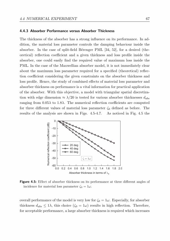
4.4 NUMERICAL EXPERIMENT 67
4.4.3 Absorber Performance versus Absorber Thickness
The thickness of the absorber has a strong influence on its performance. In ad-dition, the material loss parameter controls the damping behaviour inside theabsorber. In the case of split-field Berenger PML [34, 52], for a desired (the-oretical) reflection coefficient and a given thickness and loss profile inside theabsorber, one could easily find the required value of maximum loss inside thePML. In the case of the Maxwellian absorber model, it is not immediately clearabout the maximum loss parameter required for a specified (theoretical) reflec-tion coefficient considering the given constraints on the absorber thickness andloss profile. Hence, the study of combined effects of material loss parameter andabsorber thickness on performance is a vital information for practical applicationof the absorber. With this objective, a model with triangular spatial discretiza-tion with edge dimension ≈ λ/20 is tested for various absorber thicknesses dabsranging from 0.05λ to 1.8λ. The numerical reflection coefficients are computedfor three different values of material loss parameter ζ0 defined as before. Theresults of the analysis are shown in Figs. 4.5-4.7. As noticed in Fig. 4.5 the
Figure 4.5: Effect of absorber thickness on its performance at three different angles ofincidence for material loss parameter ζ0 = 1ω.
overall performance of the model is very low for ζ0 = 1ω. Especially, for absorberthickness dabs ≤ 1λ, this choice (ζ0 = 1ω) results in high reflection. Therefore,for acceptable performance, a large absorber thickness is required which increases
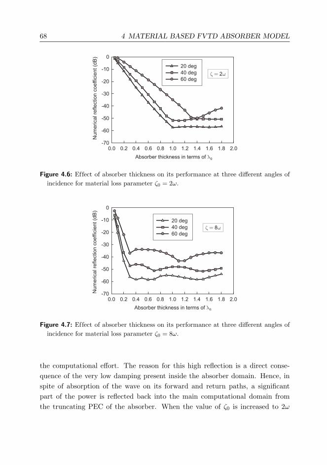
68 4 MATERIAL BASED FVTD ABSORBER MODEL
Figure 4.6: Effect of absorber thickness on its performance at three different angles ofincidence for material loss parameter ζ0 = 2ω.
Figure 4.7: Effect of absorber thickness on its performance at three different angles ofincidence for material loss parameter ζ0 = 8ω.
the computational effort. The reason for this high reflection is a direct conse-quence of the very low damping present inside the absorber domain. Hence, inspite of absorption of the wave on its forward and return paths, a significantpart of the power is reflected back into the main computational domain fromthe truncating PEC of the absorber. When the value of ζ0 is increased to 2ω
4.5 CONCLUSIONS 69
and 8ω the damping inside the absorber is substantially increased resulting inimprovement in the performance as shown in Fig. 4.6 and Fig. 4.7. The oscilla-tions noticed in the numerical reflection coefficient value in Fig. 4.7 correspondto constructive and destructive interferences between waves reflected at the FS-Ainterface and at the truncating PEC. For low values of material loss parameter(for example, as in Fig. 4.5) these oscillations are not observed due to the largeundamped reflection originating from the truncating PEC which is many ordershigher than the reflection from the initial FS-A interface. This analysis indicatesthat, by choosing a large value of ζ0 typically in the range of 8ω, one could optfor an absorber thickness smaller than 0.5λ. When the value of ζ0 is increasedbeyond a certain limit (≈ 40ω), stability problems were encountered which setsa maximum limit in choosing ζ0 for practical applications.
4.5 Conclusions
A novel approach to model the Maxwellian absorber in the framework of theFVTD method on unstructured grids has been presented. The modified formu-lation adapts naturally to the FVTD algorithm. The proposed model was testedfor angular performance under different damping conditions. For a variation ofthe angle of incidence, from near normal to 50 degree, the worst-case reflectioncoefficient of the FVTD-Maxwellian absorber is lower than −40 dB. The accu-racy of the proposed model was found to further increase when employed onmeshes finer than the present ones. Numerical reflection coefficients in the rangeof −70 dB was achieved on fine meshes confirming convergence.

70

5 Unified Finite-Volume Absorber Modelling
Abstract — Different implementations of perfectly matched absorbers are studied under the
unified framework of the finite-volume time-domain method. This comparative analysis al-
lows to discuss the similarities existing between these models and explores the differences in
their practical implementation. The theoretical development and numerical performance of
these models are presented. Analysis on the formulation highlights the theoretical equiva-
lence of the non-Maxwellian (split-field) absorbers to the Maxwellian (unsplit-field) absorbers.
Numerical experiments further confirm the theoretical equivalence between absorber mod-
els. The performance of one of the Maxwellian absorber model based on complex frequency
shifting approach is found to be better than other models in the evanescent wave region.
However, this performance improvement comes at the cost of increased computational re-
sources.
5.1 Introduction
Different implementations of the PML technique were reported in the litera-ture giving rise to two general classes, namely non-Maxwellian absorbers andMaxwellian absorbers. A typical example of non-Maxwellian absorber is thesplit-field B-PML discussed in Chap. 3. A modified Lorentz material basedMaxwellian absorber model M-PML was discussed in Chap. 4. The present chap-ter extends the analysis to two further implementations of Maxwellian absorbermodel, namely generalized theory based PML (GT-PML) [38] and the complexfrequency shifted PML (CFS-PML) [58, 59] for the FVTD simulation. In ad-dition, the theory of four different PML techniques, namely B-PML, M-PML,GT-PML, and CFS-PML are studied under a unified notation in the FVTDframework. Their formulation and numerical performance are compared in the2D TE formulation, without loss of generality.
71
72 5 UNIFIED FVTD ABSORBER MODELLING
5.2 Non-Maxwellian Absorbers
5.2.1 Berenger PML - (B-PML)
The theory and FVTD implementation of B-PML was introduced in Chap. 3.The final FVTD update equations for the B-PML can be written in the followingform
∂tUi = − 1α|Vi|
f∑k=1
(nk · FU∗k |Sk|)− L (5.1)
where Vi denotes the volume of the ith cell (control-volume) and Sk correspondsto the area of its kth face. The normal vector to the kth face is denoted nk.The field vector U is given by U = [Hx, Hy, Ez, Ezy]T , the material parametersare contained in the diagonal matrix α having the form α = diag[µi, µi, εi, εi].The term ‘n · F(·)’ corresponds to the flux-function. The ‘*’ in the subscriptindicates that the computed flux-function across each edge which depends onthe field quantities at the edge-centre. The field values at the edge-centre areapproximated with the help of corresponding cell-centre field values using thesecond-order accurate MUSCL algorithm [31]. The losses in the PML layers arerepresented by the vector L which, in theory, is derived to obtain reflectionlessabsorption for all angles, frequencies, and polarizations of the incident wave. Inthe case of B-PML, the vector L used in the FVTD update equations for perfectlymatched absorption is written as,
L =
0
(σx/εi)Hyi
(σx/εi)(Ezi − Ezyi)
0
. (5.2)
It is worth mentioning that, in the above update equations, the fourth fieldequation for Ezy constitute the non-hyperbolic part of the system and requiresspecial treament for its update. A stable update flux for Ezy is obtained byemploying the Rankine-Hugoniot jump relation discussed in Chap. 3.

5.3 MAXWELLIAN ABSORBERS 73
5.3 Maxwellian Absorber Models
5.3.1 Modified Lorentz Material-based PML - (M-PML)
The FVTD implementation of the M-PML adapted for unstructured grid confor-mal time-domain simulation is discussed in detail in Chap. 4. The final systemof update equations inside the M-PML model is given by
∂tHx = − 1µ∂yEz + ζHx −Gx (5.3)
∂tHy =1µ∂xEz − ζHy (5.4)
∂tEz =1ε
(∂xHy − ∂yHx)− ζEz (5.5)
∂tGx = −ζGx + ζ2Hx (5.6)
where ζ is the material loss-parameter inside M-PML. The fourth equation (5.6)is an ordinary differential equation in time and hence requires no special fluxfunction computation. Also the inherent structure of the Maxwellian system withthree field components, namely Hx, Hy and Ez is preserved and there is onlyan auxiliary equation for the field component Gx which has no extra overheadcompared to the B-PML model discussed in the previous section. The abovesystem of equations results in the FVTD update equations similar in form tothat of (5.1) but with a different field-vector given by U = [Hx, Hy, Ez, Gx]T andthe corresponding lossy PML field vector L given by
L =
Gxi − ζHxi
ζHyi
ζEzi
ζGxi − ζ2Hxi
. (5.7)
5.3.2 Generalized Theory based PML - (GT-PML)
In the present section, the analytical formulation of GT-PML based on the ap-proach of coordinate streching introduced in [38] is derived from the theory of
74 5 UNIFIED FVTD ABSORBER MODELLING
M-PML discussed in the previous section. The M-PML update equations con-tain an auxiliary field along with three main Maxwellian fields. Integrating theupdate equation of Gx (5.6) in time gives∫
(∂tGx)dt =∫
(−ζGx + ζ2Hx)dt . (5.8)
Now substituting Gx = Kx + ζHx in (5.3) and (5.8) result in the following
∂tHx = − 1µ∂yEz −Kx (5.9)∫
(∂tKx)dt = −ζ∫
(Kx)dt− ζ∫∂tHxdt . (5.10)
Substituting (5.9) in (5.10) gives
Kx =ζ
µ
∫∂yEzdt . (5.11)
Using (5.11) in (5.9) and appending the update equations for the two other fields,namely Hy and Ez, the final M-PML system equations can be written as follows
∂tHx = − 1µ∂yEz −
ζ
µ
t∫0
(∂yEz)dt (5.12)
∂tHy =1µ∂xEz − ζHy (5.13)
∂tEz =1ε
(∂xHy − ∂yHx)− ζEz . (5.14)
The above M-PML description employs the integration in time procedure for theHx field instead of the auxiliary equation form discussed before. This correspondsexactly to the same set of update equations obtained in the case of the GT-PML introduced in [38], however based on a different physical interpretation. Infact, the above discussion confirms the equivalence in the analytical formulationand computational load of M-PML and GT-PML. However, the implementationprocedures of these PML models influences their numerical performance whichis studied in the following section. In the notation of (5.1), the field vector forGT-PML is given by U = [Hx, Hy, Ez]T and the corresponding lossy PML vector
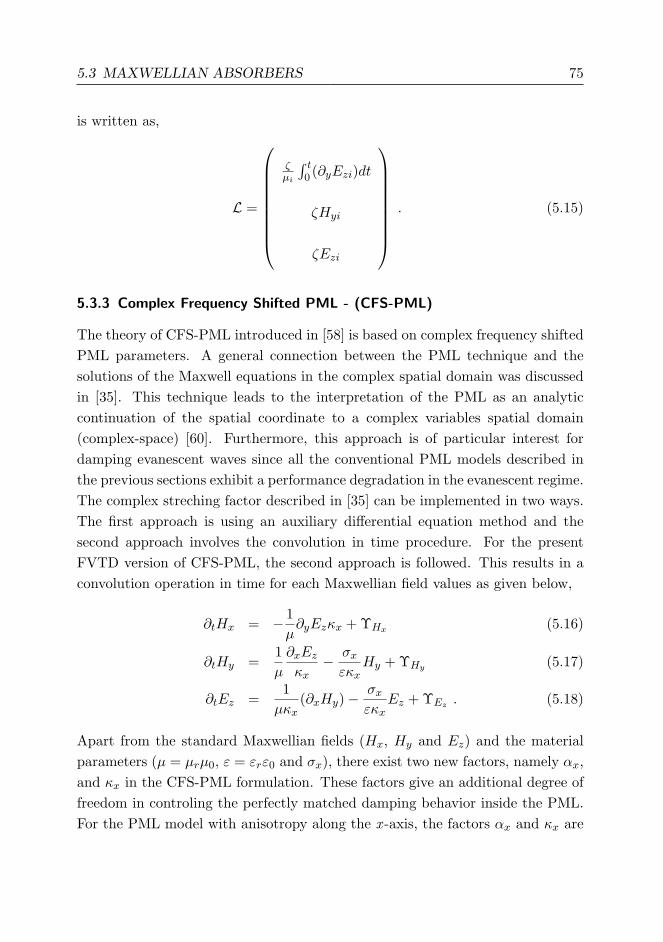
5.3 MAXWELLIAN ABSORBERS 75
is written as,
L =
ζµi
∫ t0 (∂yEzi)dt
ζHyi
ζEzi
. (5.15)
5.3.3 Complex Frequency Shifted PML - (CFS-PML)
The theory of CFS-PML introduced in [58] is based on complex frequency shiftedPML parameters. A general connection between the PML technique and thesolutions of the Maxwell equations in the complex spatial domain was discussedin [35]. This technique leads to the interpretation of the PML as an analyticcontinuation of the spatial coordinate to a complex variables spatial domain(complex-space) [60]. Furthermore, this approach is of particular interest fordamping evanescent waves since all the conventional PML models described inthe previous sections exhibit a performance degradation in the evanescent regime.The complex streching factor described in [35] can be implemented in two ways.The first approach is using an auxiliary differential equation method and thesecond approach involves the convolution in time procedure. For the presentFVTD version of CFS-PML, the second approach is followed. This results in aconvolution operation in time for each Maxwellian field values as given below,
∂tHx = − 1µ∂yEzκx + ΥHx (5.16)
∂tHy =1µ
∂xEzκx− σxεκx
Hy + ΥHy (5.17)
∂tEz =1µκx
(∂xHy)−σxεκx
Ez + ΥEz . (5.18)
Apart from the standard Maxwellian fields (Hx, Hy and Ez) and the materialparameters (µ = µrµ0, ε = εrε0 and σx), there exist two new factors, namely αx,and κx in the CFS-PML formulation. These factors give an additional degree offreedom in controling the perfectly matched damping behavior inside the PML.For the PML model with anisotropy along the x -axis, the factors αx and κx are

76 5 UNIFIED FVTD ABSORBER MODELLING
related to the complex permeability and permittivity tensor given by [58, 59]
ε = ε [Λ], µ = µ [Λ] with [Λ] =
ωx−1 0 0
0 ωx 0
0 0 ωx
(5.19)
where
ωx = κx +σx
αx + jωε. (5.20)
The terms ΥHx , ΥHy and ΥEz present in (5.16)-(5.18) are the factors due to theconvolution operation in time for each field values and they are given by,
ΥHx = − 1µ
σxεe−
αxε·t ?
f∑k=1
(FHx .nk)|Sk| (5.21)
ΥHy =αxσxκxε2
e−αxε·t ? Hy (5.22)
ΥEz =αxσxκxε2
e−αxε·t ? Ez . (5.23)
These additional convolution operations eventually make the CFS-PML highlyefficient to absorb evanescent waves at the cost of increased computational effort.It can be shown that, when κx = 1 and αx = 0, the CFS-PML formulation willbe identical to the GT-PML formulation discussed before. Hence, the CFS-PMLcan be considered as the generalization of the GT-PML.
5.4 Numerical Performance Comparison
The broadband performance of all the four PML models is compared with thatof first-order accurate SM-ABC. The numerical experiments consider the trun-cation of a parallel-plate-waveguide operated in its fundamental TE mode. Abroadband Gaussian pulse is used as the source excitation to study the numeri-cal reflection coefficient over a frequency bandwidth exceeding a 1:30 ratio. Thespatial discretization employed for the model problem corresponds to λl/6 andλh/200 at the highest (λl) and lowest (λh) frequency components of the input

5.4 NUMERICAL PERFORMANCE COMPARISON 77
Figure 5.1: Broadband performance of different FVTD-PML models in comparison withtheoretical value in a parallel-plate-waveguide.
signal, respectively. It should be noted that λl and λh correspond to the free-space wavelengths. The results obtained from all the PML models are plottedin Fig. 5.1. The frequency range under investigation spans both the evanescentand propagation regions of the input signal. In this experiment the influence ofthe angle of incidence is also addressed since the cut-off frequency correspondsto the grazing incidence whereas for higher frequencies, the angle of incidenceconverges towards normal incidence. It can be clearly noticed that at higherfrequencies (tending towards normal incidence) the performance of the SM-ABCapproaches that of the other PML models. Furthermore, at higher frequenciesthe effect of mesh discretization becomes crucial and degrades the overall per-formance of all the PML models. However, in all cases the PML models areperforming considerably better than SM-ABC. At low frequencies the angle ofincidence converge towards grazing incidence and hence, the performance of allthe models degrades in spite of very fine spatial discretization present at thosefrequencies. As expected, the results confirm that the performance of CFS-PMLin the evanescent regime is substantially better compared to other PML models,however, at the cost of increased computational load.

78 5 UNIFIED FVTD ABSORBER MODELLING
5.5 Conclusion
In the present study different PML techniques were modelled in the unified frame-work of the FVTD method. Analysis on the formulation was performed to high-light the theoretical equivalence between the absorber models. In particular, thetheoretical equivalence of M-PML and GT-PML was discussed. Numerical per-formances of all the PML models were found to be almost identical. The slightdifferences are mainly due to the different implementation procedures followed inthe PML models. As expected, the performance of the CFS-PML was substan-tially better in the evanescent wave region compared to other PML models. Thisimproved performance of CFS-PML was achieved at the cost of increased com-putational load. Although the analysis and results presented here were obtainedin the FVTD framework, the models investigated can be naturally generalizedto other conformal time-domain methods.
6 Radial Perfectly Matched Absorber Modelling
Abstract — The uniaxial finite-volume Maxwellian absorber used as an unsplit PML is ex-
tended to incorporate radial anisotropy for modelling cylindrical geometries. Theoretical
background and practical application of the radial absorber in an unstructured mesh are pre-
sented. The accuracy of the radial absorber is tested for cylindrical mesh truncation using
a representative problem involving two different test scenarios. Results are compared with
the SM-ABC demonstrating substantial reduction in numerical error due to cylindrical mesh
truncation.
The present implementation of the radial absorbers avoid corner regions which are the ma-
jor source of reflection errors in the standard Cartesian PML models, however, it is observed
that there is a significant influence of the radius of absorber curvature on its performance.
A rigourous investigation on the influence of the radius of curvature is presented using a
waveguide and a horn-antenna truncation problem. In addition, the convergence of the re-
sults is studied for increasing radius of curvature of the absorber. Low-level effects on the
antenna radiation patterns further illustrates the convergence of the technique.
6.1 Introduction
A finite-volume based uniaxial Maxwellian absorber was introduced in Chap. 4with an application to a waveguide truncation problem. For scattering and an-tenna applications, this uniaxial model suffers from inaccuracies originating fromthe corner regions which are the major sources of numerical reflections (inaccu-racies) in the computed solution. Therefore to avoid the corner regions, a radialabsorber model is introduced in this chapter. This radial Maxwellian absorbermodel uses a novel approach to achieve anisotropy in the radial direction and canbe efficiently used in applications involving cylindrical or spherical geometries.The theory of the radial absorber is developed as an extension to the uniaxialmodel and supporting numerical experiments are presented. Using curvilinearPML models, the corner regions can be avoided in the computational domain.The curvilinear PML models reported in [61, 62, 63, 64, 65, 66] were adapted
79
80 6 RADIAL PERFECTLY MATCHED ABSORBER MODELLING
mainly for FDTD and FETD methods which uses update equations representedin cylindrical coordinate. The new finite-volume radial absorber model intro-duced in this chapter is based on a different approach which capitalizes on thecapability of the FVTD method to handle unstructured mesh to its full advan-tage. Hence, the modelling of cylindrical geometry becomes possible withoutthe need for coordinate transformation as in the case of FDTD simulations.Achieving radial anisotropy using Cartesian domain formulation involves rota-tional transformation from locally uniaxial to globally radial behaviour of thematerial loss parameter.
The influence of the radius of curvature of the radial absorber model is ex-amined. Although, the radial PML technique for the FVTD method has theadvantage of simplified update equations, reduced computational domain andgeometry-matched modelling for cylindrical and elongated structures, it is ob-served that the radius of curvature of the radial absorber has a noticable influenceon its performance. Hence, this chapter further explores the accuracy limitationsof the radial absorber based on its radius of curvature and examines the usabilityof the model for studying practical problems. The numerical experiment used toinvestigate the influence of radius of curvature consists of a horn-antenna prob-lem. Numerical reflection error and its effect on the computed radiation patternare analyzed for different radii of curvature of the absorber.
6.2 Radial Finite-Volume Maxwellian Absorber
The concept of radially anisotropic cylindrical PML was reported in the frame-work of FDTD in [61, 62, 65] and for FETD applications in [66]. All theseprevious attempts in modelling cylindrical PML were motivated by represent-ing Maxwell equations in the cylindrical coordinate system. The feature of theunstructured spatial discretization enables the FVTD method to model domainboundaries of any shape in a generalized manner. Consequently, there is no needfor a special type of mesh arrangement like a curvilinear mesh and thus trans-forming the system update equations to a cylindrical coordinate system is notrequired. In the following, the theory of radial finite-volume absorbers is dis-cussed in detail and various test scenarios in cylindrical geometry are simulated.

6.2 RADIAL FINITE-VOLUME MAXWELLIAN ABSORBER 81
6.2.1 Radial Anisotropy: Rotated Coordinate Analysis
The direction of wave attenuation inside the absorber is given by the direction ofanisotropy. In the previous discussion on the uniaxial material absorber model,the anisotropy direction was chosen along the +x -axis. In contrast, when con-
Figure 6.1: Graphical illustration of radial anisotropy using coordinate transformationby rotation.
sidering a radial absorber model described in the cylindrical coordinate system(ρ, ϕ, z), the anisotropy is defined in the radial direction ρ. In other words, asillustrated in Fig. 6.1, the local direction of anisotropy is along the +xr directionand the local coordinate (xr, yr, z ) can be viewed as a rotational transformationof the global coordinate (x, y, z ) through an angle ϕ in the xy-plane.
6.2.2 Definition of Anisotropic Losses: Comparison to Standard Approach
The key differences in the definition of anisotropic losses in the standard rect-angular PML and the radial absorber are discussed in the following. In general,the direction of anisotropy inside the PML medium uniquely defines the direc-tion of attenuation of the incident wave. Hence, as discussed in the last chapter,when employing the rectangular PML for truncating a 2D computational domainconsisting of scatterers or antennas, three different types of uniaxial perfectlymatched media are necessary. As shown in Fig. 6.2, the first and second typescorrespond to uniaxial PMLs in which the directions of anisotropy are only alongthe x and y axes, respectively. The third type consists of a PML model wherewave attenuation is along both the x and y axes. The level attenuation in x andy directions are uniquely determined by the geometrical location of the pointinside the computational domain. In fact, it makes more sense to consider, the

82 6 RADIAL PERFECTLY MATCHED ABSORBER MODELLING
Figure 6.2: Left: Three different kinds of uniaxial medium used in rectangular PML.Right: Concept of local to global transformation used in radial absorber theory. Cor-responding directions of anisotropy are given with the damping coefficient. DottedLines: Common area of the computational domain.
third type of PML medium in the overlapping or corner regions as an anisotropytransformer. For accurate modelling using standard rectangular PML models,there should always be a buffer region consisting of type three PML mediumbetween any type one and type two PML regions. However, this corner regionsresult in dominant reflections from the rectangular PML models [55]. A simpleway to avoid corner regions is to employ radial (spherical) PML models whichhave the direction of anisotropy always defined along the radial direction. Infact, this globally radial behaviour can be modelled using locally uniaxial PMLmodels with the help of local to global transformation in field update equations.
6.2.3 Field Update Equations
For the assumed TE formulation, the magnetic and electric field components inthe rotated axes are given by Ur = [Hxr , Hyr , Ez]T . As clearly noticed, the rota-tional transformation in the xy-plane has no effect on the electric field componentEz along the z -axis. The field transformation from the global to the local axes

6.2 RADIAL FINITE-VOLUME MAXWELLIAN ABSORBER 83
is given by
Hxr
Hyr
Ez
=
R︷ ︸︸ ︷
cosϕ sinϕ 0
− sinϕ cosϕ 0
0 0 1
Hx
Hy
Ez
(6.1)
where R denotes the rotation matrix defined by the angle of rotation ϕ [67, 68].The system of equations in the local coordinate is written as [69],
µ0 ∂tHxr = −∂yrEz − µ0Kxr (6.2)
µ0 ∂tHyr = ∂xrEz − µ0ζxrHyr (6.3)
ε0 ∂tEz = ∂xrHyr − ∂yrHxr − ε0ζxrEz (6.4)
µ0 ∂tKxr = ζxr∂yrEz . (6.5)
Apart from the standard field vectors defined in Ur, there is a scalar field givenby Kxr which represents the magnetic counterpart of polarization current asdefined in [55] and [69]. The above set of update equations differ from thatof the uniaxial absorber (4.10)-(5.6) with respect to the fourth scalar field Kxr .Here the update equation of the fourth field is represented as a partial differentialequation (PDE) in space and time variables. In fact, one could also define thefourth field update equation as an ODE in time as discussed in Sec. 4.2. Buthere the usage of a PDE form of the update equation instead of an ODE ensuresmathematical simplicity in modelling radial anisotropy. Numerically, once theflux function of Hxr is known, the flux function of Kxr is directly obtained fromthat of Hxr with an appropriate change of sign. In order to model the radialanisotropy using the field vectors U and Kx defined in the global coordinate (x,y, z ), all the local field quantities inside each control-volume must be transformedback to the global coordinate system. This reverse transformation from local toglobal coordinate system is achieved using the following relation,
[xr, yr, z]TR−1
=⇒ [x, y, z]T . (6.6)

84 6 RADIAL PERFECTLY MATCHED ABSORBER MODELLING
Similarly, the field quantities in the local coordinate should be transformed tothe global coordinate as follows,
[Hxr , Hyr , Ez,Kxr ]T R−1
=⇒ [Hx, Hy, Ez,Kx]T . (6.7)
For complete modelling of the radial anisotropy in the global coordinate, thepartial derivatives (∂xr , ∂yr) present in (6.2)-(6.5) should be transformed backto the global coordinate using the chain rule as follows,
∂xr = ∂xr(x) ∂x + ∂xr(y) ∂y (6.8)
∂yr = ∂yr(x) ∂x + ∂yr(y) ∂y . (6.9)
Substituting (6.6) in (6.8) and (6.9) results in the following,
∂xr = cosϕ ∂x + sinϕ ∂y (6.10)
∂yr = − sinϕ ∂x + cosϕ ∂y . (6.11)
Using (6.10)-(6.11) in (6.7) and after some algebraic manipulations, all the fieldcomponents inside the radial absorber can be expressed as follows,
µ0 ∂tHx = −∂yEz + ζxrµ0Hy cosϕ sinϕ (6.12)
−ζxrµ0Hx sin2 ϕ− µ0Kxr cosϕ
µ0 ∂tHy = ∂xEz + ζxrµ0Hx cosϕ sinϕ (6.13)
−ζxrµ0Hy cos2 ϕ− µ0Kxr sinϕ
ε0 ∂tEz = ∂xHy − ∂yHx − ζxrε0Ez (6.14)
µ0 ∂tKxr = −ζxr sinϕ∂xEz + ζxr cosϕ∂yEz . (6.15)
Comparing (6.2)-(6.4) with (6.12)-(6.14), it is noticed that, the transformationfrom the local coordinates to the global coordinates does not change the structureof Maxwell equations except for the lower order terms (terms with no spatial-derivatives). This is a direct consequence of rotational invariance of the Maxwellsystem [70]. Logically the fourth scalar field Kxr should also be split into twocomponents in x and y directions. But in the system of update equations (6.12)-(6.15), this fourth field can still be represented in the local coordinate system.It should be also noticed that, the RHS of the fourth update equation (6.15) isrepresented in global coordinates. This mathematical manipulation is deliberate

6.2 RADIAL FINITE-VOLUME MAXWELLIAN ABSORBER 85
in order to use four instead of five update equations. There are clearly twoextreme situations which can be directly tested from the above update equations(6.12)-(6.15), namely ϕ = 0 and ϕ = 90 degrees. These two situations yieldupdate equations corresponding to uniaxial in +x and +y directions, respectively.Finally, the system of equations representing the radial absorber model is writtenusing the flux-based FVTD update equations as follows,
∂tHx =−1µ0|Vi|
f∑k=1
(FHxk · nk |Sk|)−Kxr cosϕ (6.16)
−ζxrHx sin2 ϕ+ ζxrHy cosϕ sinϕ
∂tHy =−1µ0|Vi|
f∑k=1
(FHyk · nk|Sk|)−Kxr sinϕ (6.17)
−ζxrHy cos2 ϕ+ ζxrHx cosϕ sinϕ
∂tEz =−1ε0|Vi|
f∑k=1
(FEzk · nk|Sk|)− ζxrEz (6.18)
∂tKxr = ζxr sinϕ1
µ0|Vi|
f∑k=1
(FHyk · nk|Sk|) (6.19)
+ζxr cosϕ1
µ0|Vi|
f∑k=1
(FHxk · nk |Sk|)
Interestingly, the flux terms computed for (6.16) and (6.17) can be reused in(6.19) and this flux-recycling helps in reducing computational effort.
6.2.4 Numerical Experiments
For testing the radial finite-volume absorber formulation, a test problem is cho-sen and as before two models (test and reference) are created (Fig. 6.3). For allthe experiments carried out in this section, the thickness of the absorber dabsis fixed to 0.5λ and the material loss parameter ζ0 is fixed to 8ω. These val-ues are chosen from the results of the uniaxial absorber model discussed before(refer to Fig. 4.7). The spatial discretization employed in the following problemcorresponds to triangular cells with edge dimensions ≈ λ/30. Two representa-tive numerical experiments were carried out as illustrated in Fig. 6.4. In thefirst example, the 2D model of the cylindrical domain is excited with an axial
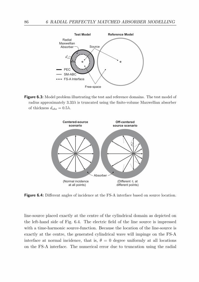
86 6 RADIAL PERFECTLY MATCHED ABSORBER MODELLING
Figure 6.3: Model problem illustrating the test and reference domains. The test model ofradius approximately 3.33λ is truncated using the finite-volume Maxwellian absorberof thickness dabs = 0.5λ.
Figure 6.4: Different angles of incidence at the FS-A interface based on source location.
line-source placed exactly at the centre of the cylindrical domain as depicted onthe left-hand side of Fig. 6.4. The electric field of the line source is impressedwith a time-harmonic source-function. Because the location of the line-source isexactly at the centre, the generated cylindrical wave will impinge on the FS-Ainterface at normal incidence, that is, θ = 0 degree uniformly at all locationson the FS-A interface. The numerical error due to truncation using the radial
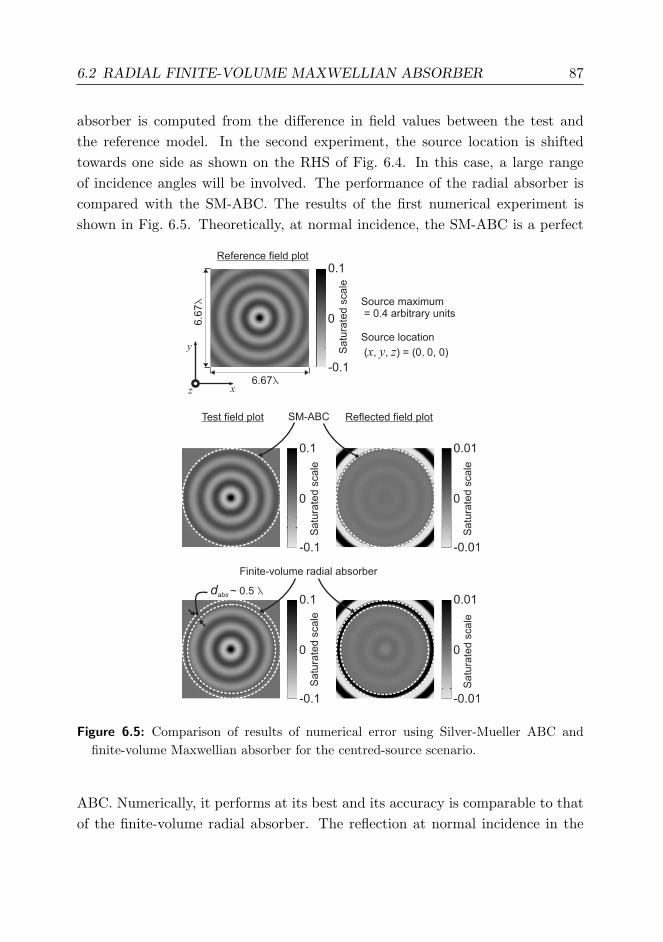
6.2 RADIAL FINITE-VOLUME MAXWELLIAN ABSORBER 87
absorber is computed from the difference in field values between the test andthe reference model. In the second experiment, the source location is shiftedtowards one side as shown on the RHS of Fig. 6.4. In this case, a large rangeof incidence angles will be involved. The performance of the radial absorber iscompared with the SM-ABC. The results of the first numerical experiment isshown in Fig. 6.5. Theoretically, at normal incidence, the SM-ABC is a perfect
Figure 6.5: Comparison of results of numerical error using Silver-Mueller ABC andfinite-volume Maxwellian absorber for the centred-source scenario.
ABC. Numerically, it performs at its best and its accuracy is comparable to thatof the finite-volume radial absorber. The reflection at normal incidence in the
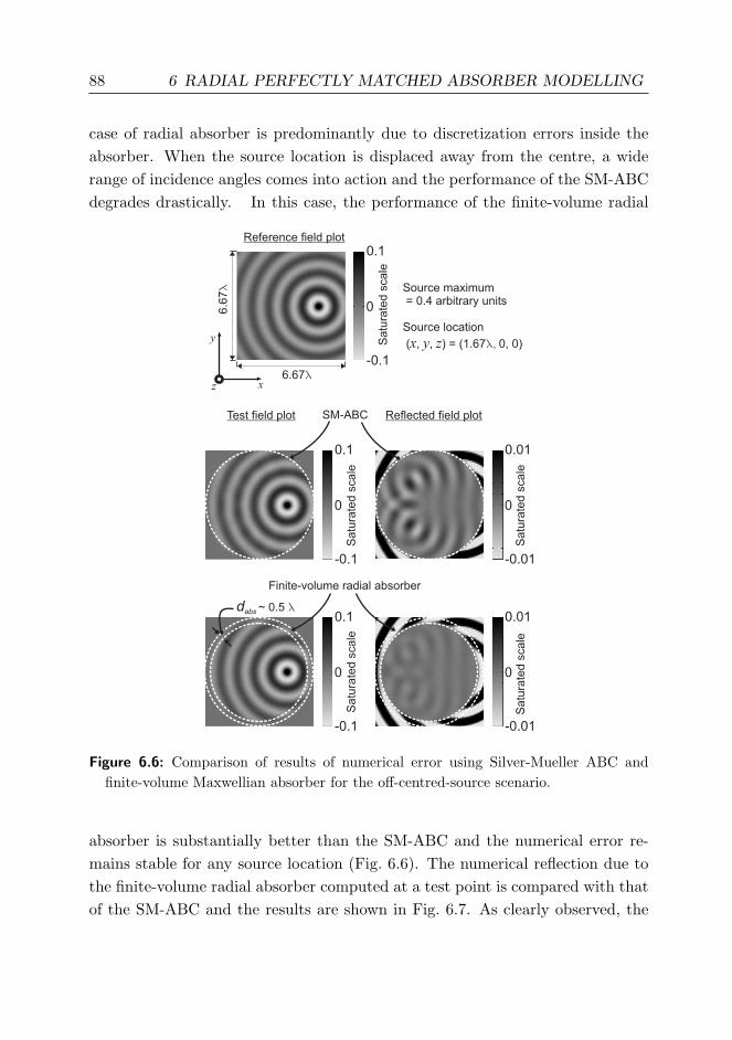
88 6 RADIAL PERFECTLY MATCHED ABSORBER MODELLING
case of radial absorber is predominantly due to discretization errors inside theabsorber. When the source location is displaced away from the centre, a widerange of incidence angles comes into action and the performance of the SM-ABCdegrades drastically. In this case, the performance of the finite-volume radial
Figure 6.6: Comparison of results of numerical error using Silver-Mueller ABC andfinite-volume Maxwellian absorber for the off-centred-source scenario.
absorber is substantially better than the SM-ABC and the numerical error re-mains stable for any source location (Fig. 6.6). The numerical reflection due tothe finite-volume radial absorber computed at a test point is compared with thatof the SM-ABC and the results are shown in Fig. 6.7. As clearly observed, the
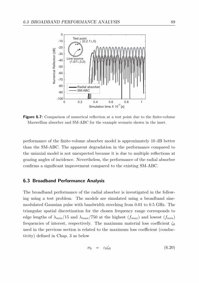
6.3 BROADBAND PERFORMANCE ANALYSIS 89
Figure 6.7: Comparison of numerical reflection at a test point due to the finite-volumeMaxwellian absorber and SM-ABC for the example scenario shown in the inset.
performance of the finite-volume absorber model is approximately 10 dB betterthan the SM-ABC. The apparent degradation in the performance compared tothe uniaxial model is not unexpected because it is due to multiple reflections atgrazing angles of incidence. Nevertheless, the performance of the radial absorberconfirms a significant improvement compared to the existing SM-ABC.
6.3 Broadband Performance Analysis
The broadband performance of the radial absorber is investigated in the follow-ing using a test problem. The models are simulated using a broadband sine-modulated Gaussian pulse with bandwidth streching from 0.01 to 0.5 GHz. Thetriangular spatial discretization for the chosen frequency range corresponds toedge lengths of λmin/15 and λmax/750 at the highest (fmax) and lowest (fmin)frequencies of interest, respectively. The maximum material loss coefficient ζ0
used in the previous section is related to the maximum loss coefficient (conduc-tivity) defined in Chap. 3 as below
σ0 = ε0ζ0 (6.20)

90 6 RADIAL PERFECTLY MATCHED ABSORBER MODELLING
Using (6.20) in the definition given in Chap. 3 (3.34), the theoretically expectedreflection coefficient can be related to the maximum loss coefficient inside theradial PML. This definition additionally helps in optimal choice of damping insidethe radial PML. In the following, instead of the material loss parameter ζxr , thelosses inside the radial PML are defined in terms of σr with maximum value givenby σ0. For all the studies carried out here, the thickness of the radial absorberis fixed to 1λmin and a quadratic profile is employed for the damping coefficientsσr. The maximum absorber damping coefficient is chosen here in order to havea theoretical reflection coefficient of −80 dB at normal incidence [34]. As a firstnumerical experiment, a centred axial line source is excited with the mentionedGaussian pulse and the domain is truncated by the radial absorber. The fieldplots at different time stamps are given in the Fig. 6.8. As second experiment,
-0.001
0.001
0S
atu
rate
dscale
Radial Absorber - Centred Source Scenario
13.3
3
min
Nearly perfectabsorption
y
z x
Sine-modulated Gaussian source(amplitude max = 0.54 arbitrary units)
y
z x
Initial focusingeffect towards
source location
t = 21.8 ns
PEC
t = 44.3 nst = 37.5 ns
d 1abs
= min
Figure 6.8: Electric field plot at different time stamps for a centred axial line sourceexcited by a broadband sine-modulated Gaussian pulse.
the axial line source is off-centred to study the performance of the absorber when

6.3 BROADBAND PERFORMANCE ANALYSIS 91
several angles of incidence are involved. The corresponding field plots at differenttime stamps are given in Fig. 6.9.
-0.001
0.001
0
Satu
rate
dscale
Radial Absorber - Off-Centred Source Scenario
13.3
3
min
Nearly perfectabsorption
y
z x
Sine-modulated Gaussian source(amplitude max = 0.54 arbitrary units)
y
z x
t = 26.3 ns
t = 44.3 nst = 37.5 ns
PEC
Initial focusingeffect fromthe source
d 1abs
= min
Figure 6.9: Electric field plot at different time stamps for an off-centred axial line sourceexcited by a broadband sine-modulated Gaussian pulse.
In the case of standard rectangular PML models, the corner regions are quitedifficult to model because there is no specified normal direction. However, asdiscussed in [55], the material parameters in the corner regions should be a simplecombination of the two side regions and the damping inside the corner regionoccurs in two orthogonal directions separately. In the case of radial absorber,the corner regions are avoided, however, the performance of the radial absorberwas found to be influenced by a focussing effect. In the presented examples ainitial focusing effect of reflected wave is observed as depicted on the top LHSillustration of Fig. 6.8 and Fig. 6.9. However, these intial reflections are nearlyperfectly absorbed in the subsequent stages.
For measuring the energy decay in the computational domains employing ra-
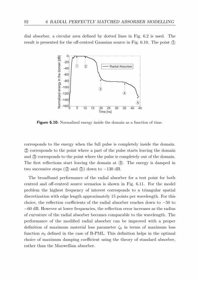
92 6 RADIAL PERFECTLY MATCHED ABSORBER MODELLING
dial absorber, a circular area defined by dotted lines in Fig. 6.2 is used. Theresult is presented for the off-centred Gaussian source in Fig. 6.10. The point 1©
Figure 6.10: Normalized energy inside the domain as a function of time.
corresponds to the energy when the full pulse is completely inside the domain.2© corresponds to the point where a part of the pulse starts leaving the domainand 3© corresponds to the point where the pulse is completely out of the domain.The first reflections start leaving the domain at 4©. The energy is damped intwo successive steps ( 2© and 5©) down to −130 dB.
The broadband performance of the radial absorber for a test point for bothcentred and off-centred source scenarios is shown in Fig. 6.11. For the modelproblem the highest frequency of interest corresponds to a triangular spatialdiscretization with edge length approximately 15 points per wavelength. For thischoice, the reflection coefficients of the radial absorber reaches down to −50 to−60 dB. However at lower frequencies, the reflection error increases as the radiusof curvature of the radial absorber becomes comparable to the wavelength. Theperformance of the modified radial absorber can be improved with a properdefinition of maximum material loss parameter ζ0 in terms of maximum lossfunction σ0 defined in the case of B-PML. This definition helps in the optimalchoice of maximum damping coefficient using the theory of standard absorber,rather than the Maxwellian absorber.

6.4 INFLUENCE OF THE RADIUS OF CURVATURE 93
0 0.1 0.2 0.3 0.4 0.5-70
-60
-50
-40
-30
-20
-10
0
Frequency [GHz]
Num
ericalR
eflection
[dB
]
CentredOff-Centred
Source location
Figure 6.11: Numerical reflection at a test point near the domain centre for both centredand off-centred source scenarios.
6.4 Influence of the Radius of Curvature
6.4.1 Uniaxial Absorber: Limiting Case of Radial Absorber
The uniaxial absorber model is actually the limiting case of the radial absorberwhen the radius of curvature (rC) approaches infinity. In other words, whenvarying rC from very small value to higher values, the radial absorber modelapproaches the uniaxial absorber model. This concept is graphically illustratedin Fig. 6.12. This limiting definition gives a geometrical view to study the in-fluence of radius of curvature on the performance. As a practical illustration ofthe limiting case concept, radial absorbers with different radius of curvature asshown in the RHS of Fig. 6.12 are used to truncate a rectangular waveguide.The objective of this numerical experiment is to study the influence of the radiusof curvature rC and compare it against theoretically expected values. Further-more, the results are compared with those of the SM-ABC. The results of thisstudy are presented in Fig. 6.13. The maximum value of the radial loss termσ0 = max(σr) = ε0ζ0 is chosen with a quadratic profile such that at normalincidence the theoretical reflection coefficient is −70 dB [34]. By using the planewave decomposition model of a waveguide mode, changing the frequency of theincident mode is equivalent to changing the angle of incidence with respect to thefree space–absorber interface. At the cut-off frequency fc the angle of incidence

94 6 RADIAL PERFECTLY MATCHED ABSORBER MODELLING
PE
C
Radial Absorber
Uniaxial Absorber
rC
PE
C
r ® ¥
Radial Uniaxial®
r rC= ¥
r rC 2
=
r rC 1
=
r r r¥ 2 1> >
PE
CP
EC
>
Figure 6.12: Left: Cylindrical domain truncation. Right: Waveguide truncation em-phasizing that the uniaxial absorber is a limiting case of radial absorber with infiniteradius of curvature.
corresponds to 90 degree and as the frequency of the incident mode increasesthe angle of incidence asymptotically reaches 0 degree. Consequently, for eachfrequency (angle of incidence), the theoretical return-loss S11 is uniquely definedfor a truncated waveguide and it is shown as dashed line in Fig. 6.13. Clearly theperformance of the SM-ABC is poor in comparison with even the radial absorberwith the smallest radius. It can be noticed that all the radial aborber modelsconverge towards the theoretically expected value of −70 dB as the frequencyof the incident mode increases. In particular, the rate of convergence is quitefast in the case of radial absorber with large radii. Furthermore, there can beanother interpretation on the convergence of the results: As the radius of curva-ture increases, the computed reflection coefficient of the radial absorber convergetowards the theoretical curve of the uniaxial absorber (rC =∞).
6.5 Numerical Experiment: Horn Antenna
The performance of the radial absorber discussed in the previous section is in-vestigated for an antenna radiation problem using radial absorbers with differentradii as shown in the Fig. 6.14. For the sake of clarity the finite thickness of the
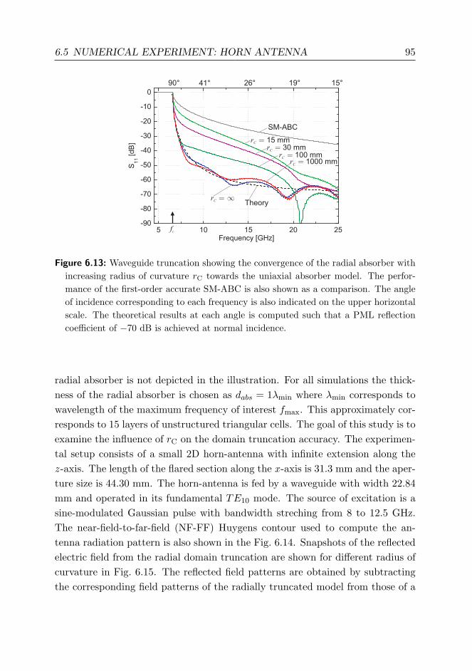
6.5 NUMERICAL EXPERIMENT: HORN ANTENNA 95
SM-ABC
rC= 30 mm
rC
= 15 mm
rC
= 100 mmr
C= 1000 mm
rC
¥=Theory
fc
90° 41° 26° 19° 15°
Figure 6.13: Waveguide truncation showing the convergence of the radial absorber withincreasing radius of curvature rC towards the uniaxial absorber model. The perfor-mance of the first-order accurate SM-ABC is also shown as a comparison. The angleof incidence corresponding to each frequency is also indicated on the upper horizontalscale. The theoretical results at each angle is computed such that a PML reflectioncoefficient of −70 dB is achieved at normal incidence.
radial absorber is not depicted in the illustration. For all simulations the thick-ness of the radial absorber is chosen as dabs = 1λmin where λmin corresponds towavelength of the maximum frequency of interest fmax. This approximately cor-responds to 15 layers of unstructured triangular cells. The goal of this study is toexamine the influence of rC on the domain truncation accuracy. The experimen-tal setup consists of a small 2D horn-antenna with infinite extension along thez -axis. The length of the flared section along the x -axis is 31.3 mm and the aper-ture size is 44.30 mm. The horn-antenna is fed by a waveguide with width 22.84mm and operated in its fundamental TE10 mode. The source of excitation is asine-modulated Gaussian pulse with bandwidth streching from 8 to 12.5 GHz.The near-field-to-far-field (NF-FF) Huygens contour used to compute the an-tenna radiation pattern is also shown in the Fig. 6.14. Snapshots of the reflectedelectric field from the radial domain truncation are shown for different radius ofcurvature in Fig. 6.15. The reflected field patterns are obtained by subtractingthe corresponding field patterns of the radially truncated model from those of a
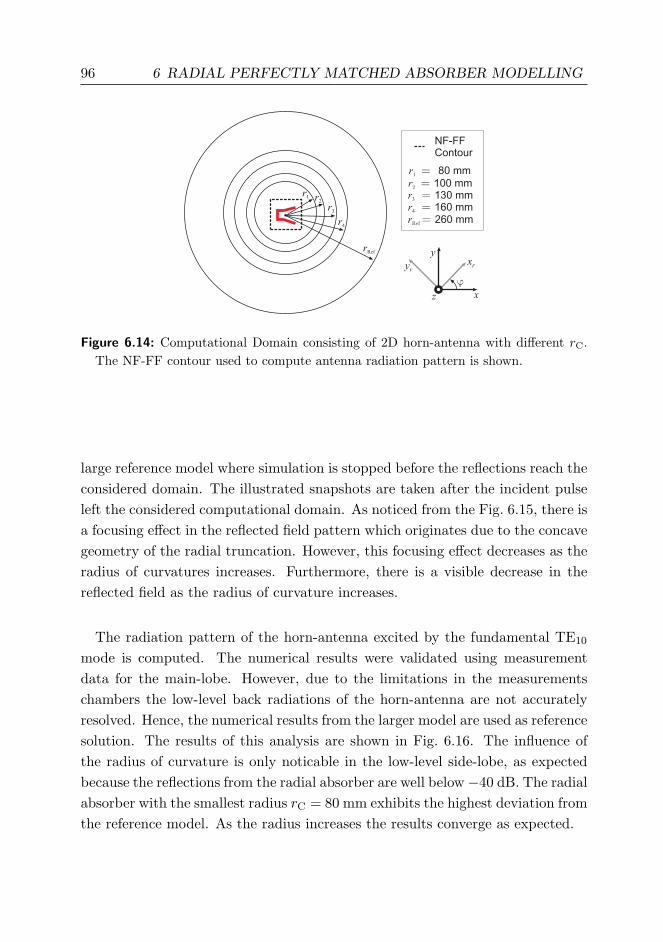
96 6 RADIAL PERFECTLY MATCHED ABSORBER MODELLING
r1
NF-FFContour
r2
r3
r4
rRef
r1
= 80 mm
r2
= 100 mmr
3= 130 mm
r4
= 160 mmr
Ref= 260 mm
x
y
xry
r
z
j
Figure 6.14: Computational Domain consisting of 2D horn-antenna with different rC.The NF-FF contour used to compute antenna radiation pattern is shown.
large reference model where simulation is stopped before the reflections reach theconsidered domain. The illustrated snapshots are taken after the incident pulseleft the considered computational domain. As noticed from the Fig. 6.15, there isa focusing effect in the reflected field pattern which originates due to the concavegeometry of the radial truncation. However, this focusing effect decreases as theradius of curvatures increases. Furthermore, there is a visible decrease in thereflected field as the radius of curvature increases.
The radiation pattern of the horn-antenna excited by the fundamental TE10
mode is computed. The numerical results were validated using measurementdata for the main-lobe. However, due to the limitations in the measurementschambers the low-level back radiations of the horn-antenna are not accuratelyresolved. Hence, the numerical results from the larger model are used as referencesolution. The results of this analysis are shown in Fig. 6.16. The influence ofthe radius of curvature is only noticable in the low-level side-lobe, as expectedbecause the reflections from the radial absorber are well below−40 dB. The radialabsorber with the smallest radius rC = 80 mm exhibits the highest deviation fromthe reference model. As the radius increases the results converge as expected.
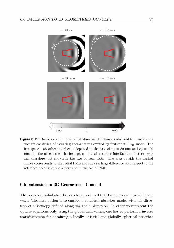
6.6 EXTENSION TO 3D GEOMETRIES: CONCEPT 97
rC= 80 mm r
C= 100 mm
rC= 160 mmr
C= 130 mm
0.004-0.004 0
PM
L
P
ML
1-1
Figure 6.15: Reflections from the radial absorber of different radii used to truncate thedomain consisting of radiating horn-antenna excited by first-order TE10 mode. Thefree-space – absorber interface is depicted in the case of rC = 80 mm and rC = 100mm. In the other cases the free-space – radial absorber interface are further awayand therefore, not shown in the two bottom plots. The area outside the dashedcircles corresponds to the radial PML and shows a large difference with respect to thereference because of the absorption in the radial PML.
6.6 Extension to 3D Geometries: Concept
The proposed radial absorber can be generalized to 3D geometries in two differentways. The first option is to employ a spherical absorber model with the direc-tion of anisotropy defined along the radial direction. In order to represent theupdate equations only using the global field values, one has to perform a inversetransformation for obtaining a locally uniaxial and globally spherical absorber

98 6 RADIAL PERFECTLY MATCHED ABSORBER MODELLING
Angle [degree]
0 45 90 135 180 225 270 315 360
-50
-40
-30
-20
-10
0
Norm
aliz
ed P
attern
[dB
]r
C= 80 mm
rC
= 100 mm
rC
= 130 mm
rC
= 160 mm
rRef
= 260 mm
f = 10 GHz
Figure 6.16: Horn-antenna radiation pattern at 10 GHz using radial absorber of differ-ent radii. The results shown nearly same results for the main-lobe of the antenna.Differences are observable in the side-lobes which are well below −40 dB. Convergencein the result is noticed as rC increases.
behaviour. Contrary to the 2D radial absorber case, the spherical transformationwill affect all the field components due to two degrees of rotation involved.
However, for elongated structures, employing a spherical absorber for domaintruncation will drastically increase the computational volume. Hence, to avoidthe computational overhead, a second option is proposed employing a cylindricalabsorber model with two hemispherical absorbers appended as the top and bot-tom cover. Without loss of generality, if the z axis is assumed to align along thelonger dimension of the enlongated structure, then a cylindrical absorber can beemployed with the z axis chosen as the axis of the absorber. Appending sphericalabsorbers on the top and bottom of the cylindrical absorber avoids corner regionsand hence, offers more accurate domain truncation. The proposed idea for 3Dextension is the topic on interest in the next chapter.
6.7 Conclusion
The uniaxial finite-volume Maxwellian absorber introduced in Chap. 4 is ex-tended for modelling cylindrical geometries. The modified formulation of theradial absorber adapts naturally to the FVTD algorithm in Cartesian coordi-nates without any need for coordinate transformation, convolution or curvilinearmeshing. The performance of the radial absorber was compared with the SM-
6.7 CONCLUSION 99
ABC. The overall performance of the radial absorber was found to be significantlybetter than the existing mesh truncation technique in the framework of FVTDmethod.
It was observed that the radius of curvature has a noticable impact on theaccuracy of the absorber. Due to the approximation in the formulation of theradial PML, a focusing effect is observed which is a trade-off for corner-reflectionsfrom standard rectangular PML. It should be stressed that, the results presentedin this chapter are only a worst-case scenario. However, reflection errors wereobserved to be in the range of −50 to −60 dB. Energy decay analysis for themodel problem demonstrated the successive damping of multiple reflections us-ing the radial absorber. For most practical applications like antenna patterncomputation, the observed reflection errors do not affect significantly the com-puted results and hence, it is possible to place the radial absorber very close tothe radiating source. Consequently, the radial absorber can aid in reducing thetotal computational domain required maintaining certain level of accuracy. Fur-thermore, the radial absorber can be used at its full advantage for applicationsinvolving very low-level coupling or scattering phenomena.

100

7 3D - Spherical Perfectly Matched Absorber Modelling
Abstract — The 2D radial PML introduced in the previous chapter is generalized to trun-
cate 3D problems using the spherical PML technique. A step-by-step procedure for deriving
the update equations inside the spherical PML starting with the geometrical definition of
rotation matrix is presented. The performance of the absorber is characterized with numer-
ical experiments and a complex problem which involves low-level coupling effects between
two spiral antennas is investigated. Simulation results confirm that the spherical absorber
technique helps in accurately resolving the low-level effects in comparison to the existing
first-order boundary conditions. Furthermore, an excellent agreement with the measurement
results validates the practical application of the technique.
7.1 Introduction
The performance of the radial PML and the simplicity of its formulation wasdiscussed in detail in the previous chapter. The radial PML can be of greathelp in modelling elongated structures in 2D and 3D applications. However, formodelling antennas or scattering problems in 3D, a spherical PML model couldbe of great value. Like in the case of radial absorber, the spherical absorber offersdomain truncation using minimal computational space, and additionally, can bemodelled using a single set of generalized update equations.
In the following, the 2D radial absorber introduced in the previous chapterfor the FVTD method is extended to the 3D radial PML model for accuratespherical domain truncation.
7.2 3D Spherical PML Models: Theory
It is very natural to truncate the computational domain for a radiation problemusing any ABC that can be modelled conformally on a spherical boundary. Avery simple approach is to use the SM-ABC technique, however, as mentioned
101
102 7 3D - SPHERICAL FVTD-PML
before this technique is only first-order accurate. For capturing very low-leveleffects, this kind of ABC should be placed very far away from the scatterer or theantenna and hence, results in increased computational effort. An accurate trun-cation is given by the radial anisotropic PML medium which can be modelled inspherical coordinates resulting in the system of update equations for the electricand magnetic field completely in spherical coordinates [62, 63]. By using theidea of transformation from locally uniaxial to globally radial PML characteris-tics introduced in the last chapter, it is possible to get an approximate system ofupdate equations completely in the Cartesian coordiate system. The reason forterming the system as approximate is due to the fact that the radial PML canbe considered as a uniaxial model projected on the spherical domain. As shownin the previous chapter, when the radius of curvature increases the radial modelconverges to its uniaxial limit.
In order to generalize the 2D cylindrical PML to 3D spherical PML, the radiallyanisotropic PML medium is considered as shown on the left-hand illustration ofFig. 7.1. The spherical PML is truncated by the PEC surface. The thickness ofthe spherical absorber dabs in the following FVTD model corresponds typically to10 unstructured cell (tetrahedral) edge lengths. This consideration is comparableto practically used PML models in the standard FDTD simulations where dabscorresponds to 10 to 15 structured cell (hexahedral) edge lengths. Depending onits geometrical position, inside the spherical PML medium, each cell is uniquelycharacterized by anisotropic PML losses.
7.2.1 Geometrical Consideration: Definition of Rotational Matrix
Each cell inside the spherical PML has two coordinate systems: The first oneis called the local coordinate system (xr, yr, zr) which is used to locally definethe uniaxial PML characteristics. The second one is called the global coordinatesystem (x, y, z ) which is used to define the global electric and magnetic fieldcomponents. In the above illustration, without loss of generality, the directionof anisotropy is chosen along the zr-axis. Furthermore, it is possible to trans-form the global coordinate system to the local one by appropriately rotating theglobal coordinate system. As opposed to 2D rotation, there exist infinitely manypossible ways of defining this rotational transformation in 3D. However, for thesake of simplicity, a simple rotational transformation is considered in this chap-

7.2 3D SPHERICAL PML MODELS: THEORY 103
Figure 7.1: A typical application of spherical domain truncation. Left: SM-ABC. Right:PML
ter which results in the transformation-matrix R from global to local axes usingtwo angles of rotation ϕ and θ. In fact, this transformation can be consideredto involve two rotations in consecutive steps as follows: The first step involvesrotation about the z -axis through an angle ϕ which will not affect the z axis,however, the x and y axes are transformed to the new rotated axes x
′r (not shown
in the Fig. 7.1 for clarity) and yr, respectively.The second step involves rotationabout the new rotated yr through an angle ϕ. In otherwords, mathematicallyspeaking, this rotational transformation can be written as follows
[xr, yr, zr]TR−1
=⇒ [x, y, z]T (7.1)
where the corresponding 3D rotational transformation matrix is given by
R−1 = RT =
cosϕ cos θ − sinϕ cosϕ sin θ
sinϕ cos θ cosϕ sinϕ cos θ
− sin θ 0 cos θ
(7.2)
7.2.2 3D FVTD Spherical PML Update Equations
The material properties of the uniaxial medium are characterized by its per-mittivity and permeability tensors which when represented in the local rotated
104 7 3D - SPHERICAL FVTD-PML
coordinate system have the form
ε = εΛr and µ = µΛr (7.3)
where (.) represents tensor matrix with anisotropy defined in the zr directiongiven by
Λr =
Ωr 0 0
0 Ωr 0
0 0 Ω−1r
, Ωr = 1 +
σrjωε
. (7.4)
The above definition is consistent with [36]. The term σr = σr(xr, yr, zr) cor-responds to the losses inside the spherical PML represented in Fig. 7.1 and itpurely depends on the geometrical position of the PML cell.
In the following derivation, the PML model based on the Maxwellian absorberformulation [55] is used. It can be proved numerically and theoretically thatthis formulation is analytically equivalent to the anisotropy based uniaxial PMLmodel introduced in [36]. For a 3D problem, the governing equations for updatingthe field values inside each radial PML cell are expressed in the local coordinatesystem as
ε0∂tExr = ∂yrHzr − ∂zrHyr − σrExr (7.5)
ε0∂tEyr = ∂zrHxr − ∂xrHzr − σrEyr (7.6)
ε0∂tEzr = ∂xrHyr − ∂yrHxr − Jzr (7.7)
µ0∂tHxr = −∂yrEzr + ∂zrHyr − σr(µ0/ε0)Hxr (7.8)
µ0∂tHyr = −∂zrExr + ∂xrHzr − σr(µ0/ε0)Hyr (7.9)
µ0∂tHzr = −∂xrEyr + ∂yrHxr − µ0Kzr (7.10)
ε0∂tJzr = −σr∂xrHyr + σr∂yrHxr (7.11)
µ0∂tKzr = (σr/ε0)∂xrEyr − (σr/ε0)∂yrExr . (7.12)
Equations (7.5)-(7.10) represent the standard Maxwell equations with additionalzeroth-order loss terms inside the PML cells. The last two equations (7.11) and(7.12) correspond to the update equations of the scalar electric Jzr and magnetic
7.2 3D SPHERICAL PML MODELS: THEORY 105
Kzr current quantities [55]. Expressing all the field quantities in the globalcoordinate system (x, y, z ) helps in modelling the spherical PML completelyin the Cartesian formulation. The field quantities in the local rotated Cartesiancoordinate are related to that in the global Cartesian through the transformationmatrix defined in (7.2) as follows
Er = R ·E, Hr = R ·H (7.13)
Jr = R · J, Kr = R ·K (7.14)
where E = [Ex, Ey, Ez]T, H = [Hx, Hy, Hz]T, J = [0, 0, Jz]T, and K = [0, 0,Kz]T
correspond to the field components in the global Cartesian coordinates. Thecorresponding fields in the rotated local coordinate system is given by Er =[Exr , Eyr , Ezr ]T, Hr = [Hxr , Hyr , Hzr ]T, Jr = [0, 0, Jzr ]T, and Kr = [0, 0,Kzr ]T.The spatial partial derivates in local and global coordinates are related to eachother as below
∂xr = cosϕ cos θ∂x + sinϕ cos θ∂y − sin θ∂z (7.15)
∂yr = − sinϕ∂x + cosϕ∂y (7.16)
∂zr = cosϕ sin θ∂x + sinϕ sin θ∂y + cos θ∂z . (7.17)
Using (7.13)-(7.17) in (7.5)-(7.10) and solving for ∂tEx, ∂tEy, ∂tEz, ∂tHx, ∂tHy
and ∂tHz yield the governing equations for all the Maxwellian field componentsinside the PML are as follows
ε0∂tEx = ∂yHz − ∂zHy − σrEx(1− cos2 ϕ sin2 θ) (7.18)
+σrEy cosϕ sinϕ sin2 θ + σrEz cosϕ cos θ sin θ
−Jzr cosϕ sin θ
ε0∂tEy = ∂zHx − ∂xHz + σrEx cosϕ sinϕ sin2 θ (7.19)
−σrEy(1− sin2 ϕ sin2 θ) + σrEz sinϕ cos θ sin θ
−Jzr sinϕ sin θ
ε0∂tEz = ∂xHy − ∂yHx + σrEx cosϕ cos θ sin θ (7.20)
+σrEy sinϕ cos θ sin θ − σrEz sin2 θ
−Jzr cos θ

106 7 3D - SPHERICAL FVTD-PML
µ0∂tHx = −∂yEz + ∂zEy − σr(µ0/ε0)Hx(1− cos2 ϕ sin2 θ) (7.21)
+σr(µ0/ε0)Hy cosϕ sinϕ sin2 θ + σr(µ0/ε0)Hz cosϕ cos θ sin θ
−µ0Kzr cosϕ sin θ
µ0∂tHy = −∂zEx + ∂xEz + σr(µ0/ε0)Hx cosϕ sinϕ sin2 θ (7.22)
−σr(µ0/ε0)Hy(1− sin2 ϕ sin2 θ) + σr(µ0/ε0)Hz sinϕ cos θ sin θ
−µ0Kzr sinϕ sin θ
µ0∂tHz = −∂xEy + ∂yEx + σr(µ0/ε0)Hx cosϕ cos θ sin θ (7.23)
+σr(µ0/ε0)Hy sinϕ cos θ sin θ − σr(µ0/ε0)Hz sin2 θ
−µ0Kzr cos θ .
In equations (7.18)-(7.23), it can be noticed on the RHS that the first two termsexactly resemble the flux-terms in the standard Maxwell equations. The otherzeroth-order (no spatial derivatives) terms correspond to the anisotropic lossesinside the PML medium. Furthermore, the last terms in (7.18)-(7.23) containJzr or Kzr and are deliberately kept in the local rotated Cartesian coordinatesystem in order to reduce the computational overhead. Using (7.13)-(7.17) in(7.11)-(7.12) results in the update equations for Jzr and Kzr are as follows
ε0∂tJzr = σr(∂zHy − ∂yHz) cosϕ sin θ (7.24)
+σr(∂xHz − ∂zHx) sinϕ sin θ
+σr(∂yHx − ∂xHy) cos θ
µ0∂tKzr = σr(1/ε)(∂yEz − ∂zEy) cosϕ sin θ (7.25)
+σr(1/ε)(∂zHx − ∂xHz) sinϕ sin θ
+σr(1/ε)(∂xHy − ∂yHx) cos θ .
Equations (7.18)-(7.25) are spatially integrated over each control-volume to ob-tain the semi-discrete FVTD update equations for all the field components insidethe spherical PML as follows
ε0∂tEx =−1|Vi|
f∑k=1
(FExk · nk |Sk|)− σrEx(1− cos2 ϕ sin2 θ) (7.26)
+σrEy cosϕ sinϕ sin2 θ + σrEz cosϕ cos θ sin θ
−Jzr cosϕ sin θ
7.2 3D SPHERICAL PML MODELS: THEORY 107
ε0∂tEy =−1|Vi|
f∑k=1
(FEyk · nk |Sk|) + σrEx cosϕ sinϕ sin2 θ (7.27)
−σrEy(1− sin2 ϕ sin2 θ) + σrEz sinϕ cos θ sin θ
−Jzr sinϕ sin θ
ε0∂tEz =−1|Vi|
f∑k=1
(FEzk · nk |Sk|) + σrEx cosϕ cos θ sin θ (7.28)
+σrEy sinϕ cos θ sin θ − σrEz sin2 θ
−Jzr cos θ
µ0∂tHx =−1|Vi|
f∑k=1
(FHxk · nk |Sk|) (7.29)
−σr(µ0/ε0)Hx(1− cos2 ϕ sin2 θ)
+σr(µ0/ε0)Hy cosϕ sinϕ sin2 θ
+σr(µ0/ε0)Hz cosϕ cos θ sin θ − µ0Kzr cosϕ sin θ
µ0∂tHy =−1|Vi|
f∑k=1
(FHyk · nk |Sk|) (7.30)
+σr(µ0/ε0)Hx cosϕ sinϕ sin2 θ
−σr(µ0/ε0)Hy(1− sin2 ϕ sin2 θ)
+σr(µ0/ε0)Hz sinϕ cos θ sin θ − µ0Kzr sinϕ sin θ
µ0∂tHz =−1|Vi|
f∑k=1
(FHzk · nk |Sk|) (7.31)
+σr(µ0/ε0)Hx cosϕ cos θ sin θ
+σr(µ0/ε0)Hy sinϕ cos θ sin θ − σr(µ0/ε0)Hz sin2 θ
−µ0Kzr cos θ
ε0∂tJzr =σr cosϕ sin θ|Vi|
f∑k=1
(FExk · nk |Sk|) (7.32)
+σr sinϕ sin θ|Vi|
f∑k=1
(FEyk · nk |Sk|)
+σr cos θ|Vi|
f∑k=1
(FEzk · nk |Sk|)

108 7 3D - SPHERICAL FVTD-PML
µ0∂tKzr =σr cosϕ sin θ
ε0|Vi|
f∑k=1
(FHxk · nk |Sk|) (7.33)
+σr sinϕ sin θ
ε0|Vi|
f∑k=1
(FHyk · nk |Sk|)
+σr cos θε0|Vi|
f∑k=1
(FHzk · nk |Sk|) .
The update equations for Jzr (7.32) and Kzr (7.33) require only the flux compo-nents which are already computed for updating the equations (7.26)-(7.31) andhence, the computational overhead for modelling the spherical PML is minimal.
7.2.3 Implementation Issues
The overall spherical PML system of equations (7.26)-(7.33) is straightforward toimplement because the flux components derived in the case of a standard FVTDmodel is directly used. Inside each cell only three PML-related parameters arerequired, namely the radial absorber conductivity σr and the two angles ϕ and θ,which are uniquely determined for each cell for the chosen direction of anisotropyalong the zr-axis. The two angles ϕ and θ in fact, correspond to the angularspherical coordinates at the barycentre of the cell. Hence, depending upon thespatial location of the cell, all the three components (σr, ϕ, θ) are uniquelydetermined and have to be computed only once in the preprocessing.
Furthermore, it should be remarked that, the system (7.26)-(7.33) can be con-sidered as a generalized formulation of the uniaxial PML with anisotropy in thedirection defined by the angles (ϕ, θ). For instance, the uniaxial PML formula-tion directed along the x, y and z axes can be obtained when the value of (ϕ,θ) in degrees correspond to (90, 0), (90, 90) and (0, 0), respectively.Hence,the standard uniaxial PML model can be interpreted as a particular case of aradial absorber with infinite radius of curvature, that is, r →∞.
7.3 Numerical Examples
In the following, three examples with increasing level of complexity are presentedto investigate and validate the performance of the 3D spherical PML model inthe framework of conformal FVTD method.

7.3 NUMERICAL EXAMPLES 109
7.3.1 Waveguide Truncation: Spherical PML with Infinite Radius of
Curvature
The 3D spherical PML model is used as an uniaxial PML model by fixing theangles (ϕ, θ) to (0, 0) degrees. As discussed before, this corresponds to uniaxialPML with direction of anisotropy along z -axis. The first example considersa WR90 rectangular waveguide with transverse waveguide dimensions as a =22.86 mm, b = 10.16 mm resulting in the cut-off frequency for the fundamentalTE10 mode of 6.56 GHz. The waveguide axis is along the z axis and it is truncatedby a 15 mm thick uniaxial PML with PEC termination. The numerical return-loss computed for the truncated waveguide is shown in Fig. 7.2 for four differentvalues of theoretical return-loss S11(f) which is a function of incident frequency.For the waveguide truncation problem, the theoretical values of S11(f) correspond
= -20 dB
= -40 dB
= -60 dB
= -80 dB
[dB
]
[GHz]
Figure 7.2: Numerical return-loss S11(f) of a WR90 rectangular waveguide truncated bya 15 mm thick uniaxial PML for different theoretical reflection-coefficent computedat normal incidence Γ0 = Γ(γ = 0). The theoretical values are computed accordingto (7.34).
to the predefined theoretically expected reflection coefficient Γ0. At the free-space–PML interface, the theoretical reflection coefficient Γ0 as a function ofincident angle γi is obtained as [34]
Γ(γi) = exp(−(2/(p+ 1))(σ0 dabs/ε0c) cos γi) (7.34)

110 7 3D - SPHERICAL FVTD-PML
where p corresponds to the loss-profile (typically quadratic, p = 2) and dabs
denotes the thickness of the radial absorber. The theoretical S11(f) at each fre-quency is represented by dashed lines in Fig. 7.2. According to the classicaldecomposition of the waveguide mode into planewaves, the angle of incidence γdepends purely on the frequency of operation f. At the cut-off frequency, theangle of incidence γ(f = fc) corresponds to 90 (grazing incidence) and as thefrequency of operation increases asymptotically towards infinity, the angle of in-cidence γ(f →∞) approaches 0. The numerical reflection-coefficient computedin this procedure corresponds to the numerical return-loss inside the truncatedwaveguide. The results plotted in Fig. 7.2 demonstrate that the 3D uniaxialPML derived from the 3D spherical PML performs as intended. The low-leveloscillations observed in the results for Γ0 = −80 dB are more likely to be dueto the numerical imperfections of the source. Furthermore, the performance ofthe spherical PML saturates below Γ0 = −80 dB due to discretization errors.For instance, decreasing Γ0 to −100 dB does not enhance the performance forthe considered spatial discretization which is about 16 points per wavelength atf = 25 GHz.
The uniaxial model is also tested for other directions of anisotropy other thanalong z -axis. The resulting uniaxial PML models performed identically for anyorientation based on (ϕ, θ) provided the axis of the waveguide is aligned alongthe direction of anisotropy in each case.
7.3.2 Spherical Domain with a Point-Source
As a second example, an infinitesimal current-source (point-source) along the z -axis is placed in a spherical computational domain. The point-source is fed witha modulated Gaussian pulse with a bandwidth strechting from 1 to 20 GHz. Thespherical computational domain with a radius of 50 mm is considered and thesource is displaced from the centre of the spherical domain in order to investigatereflections from a wide range of incident angles. Snapshots of the z -componentof the electric field at two different time-stamps are shown in Fig. 7.3 for a point-source located at x = 20 mm and y, z = 0 mm depicted as a circle with a dot inFig. 7.3. The performance of local boundary conditions for this kind of problemsis studied by truncating the spherical domain using the first-order SM-ABC andthe snapshots corresponding to this technique at two different time-stamps as
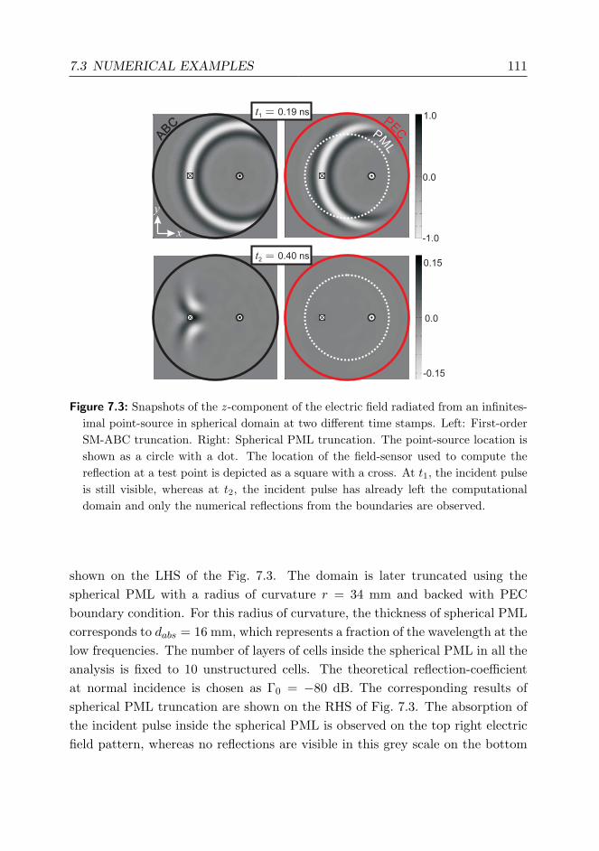
7.3 NUMERICAL EXAMPLES 111
PECPM
L
0.0
-1.0
1.0
0.0
-0.15
0.15
AB
C
AB
C
x
y
t1 = 0.19 ns
t2 = 0.40 ns
Figure 7.3: Snapshots of the z -component of the electric field radiated from an infinites-imal point-source in spherical domain at two different time stamps. Left: First-orderSM-ABC truncation. Right: Spherical PML truncation. The point-source location isshown as a circle with a dot. The location of the field-sensor used to compute thereflection at a test point is depicted as a square with a cross. At t1, the incident pulseis still visible, whereas at t2, the incident pulse has already left the computationaldomain and only the numerical reflections from the boundaries are observed.
shown on the LHS of the Fig. 7.3. The domain is later truncated using thespherical PML with a radius of curvature r = 34 mm and backed with PECboundary condition. For this radius of curvature, the thickness of spherical PMLcorresponds to dabs = 16 mm, which represents a fraction of the wavelength at thelow frequencies. The number of layers of cells inside the spherical PML in all theanalysis is fixed to 10 unstructured cells. The theoretical reflection-coefficientat normal incidence is chosen as Γ0 = −80 dB. The corresponding results ofspherical PML truncation are shown on the RHS of Fig. 7.3. The absorption ofthe incident pulse inside the spherical PML is observed on the top right electricfield pattern, whereas no reflections are visible in this grey scale on the bottom
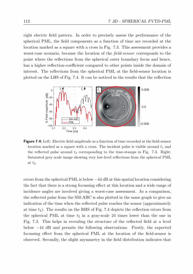
112 7 3D - SPHERICAL FVTD-PML
right electric field pattern. In order to precisely assess the performance of thespherical PML, the field components as a function of time are recorded at thelocation marked as a square with a cross in Fig. 7.3. This assessment provides aworst-case scenario, because the location of the field-sensor corresponds to thepoint where the reflections from the spherical outer boundary focus and hence,has a higher reflection-coefficient compared to other points inside the domain ofinterest. The reflections from the spherical PML at the field-sensor location isplotted on the LHS of Fig. 7.4. It can be noticed in the results that the reflection
0.0
-0.006
0.0061/24 grayscale
PECPM
L
t2
SM-ABCPML
t1
t2
[dB
]
[ns]
Figure 7.4: Left: Electric field amplitude as a function of time recorded at the field-sensorlocation marked as a square with a cross. The incident pulse is visible around t1 andthe reflected pulse around t2 corresponding to the time-stamps in Fig. 7.3. Right:Saturated grey scale image showing very low-level reflections from the spherical PMLat t2.
errors from the spherical PML is below−44 dB at this spatial location consideringthe fact that there is a strong focussing effect at this location and a wide range ofincidence angles are involved giving a worst-case assessment. As a comparison,the reflected pulse from the SM-ABC is also plotted in the same graph to give anindication of the time when the reflected pulse reaches the sensor (approximatelyat time t2). The results on the RHS of Fig. 7.4 depicts the reflection errors fromthe spherical PML at time t2 in a gray-scale 24 times lower than the one inFig. 7.3. This helps in revealing the structure of the reflected field at a levelbelow −44 dB and permits the following observations. Firstly, the expectedfocussing effect from the spherical PML at the location of the field-sensor isobserved. Secondly, the slight asymmetry in the field distribution indicates that
7.3 NUMERICAL EXAMPLES 113
the level of reflection errors are at a magnitude close to the mesh-induced noiseerrors in methods with unstructured spatial discretization. Finally, it is observedthat the low-frequency field components are decaying at a slower phase comparedto the high-frequency components because of the small radius of curvature of thespherical PML for low frequency components which results in multiple reflectionsand focusing effects.
7.3.3 Mutual Coupling between Two Archimedean Spiral Antennas
A challenging third example is used to demonstrate the practical applicationof the spherical absorber. For most antenna applications, the performance ofSM-ABC is accurate enough for obtaining results that are of practical engineer-ing value. However, for scattering problems, or for the evaluation of low-levelcoupling between devices, the reflection from the truncating boundary might be-come a dominant source of numerical error. In the following example, low-levelcoupling between two Archimedean spiral antennas placed in close proximity isconsidered. Both the Archimedean spiral antennas are cavity-backed with anoperation bandwidth of 1 to 18 GHz. A detailed FVTD modelling of one suchdevice was published recently in [71]. A very detailed and accurate modelling ofsuch devices is made possible exploiting strongly inhomogenous tetrahedral mesharrangements. Each spiral antenna model consists of the following features:
• 26 windings of the two 0.25 mm wide arms of the spiral
• 0.25 mm thick substrate
• absorber-loaded cavity and
• feeding balun
In the present investigation, the two spiral antennas are placed next to eachother in a tilted configuration as shown in Fig. 7.5. One of the spiral antennas isexcited by a wideband pulse and the coupling parameter S21 at the input portof the second spiral antenna is computed. The first analysis considers the casewhen the computational domain is truncated with the SM-ABC without sphericalPML. For a good performance, the radius of curvature of the SM-ABC, denotedas RABC, should be chosen large enough such that a near-normal incidence is
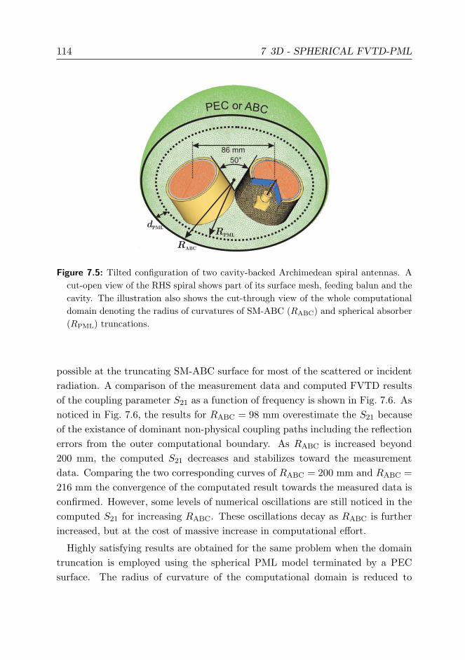
114 7 3D - SPHERICAL FVTD-PML
86 mm
50°
dPML
RABC
RPML
PEC or ABC
Figure 7.5: Tilted configuration of two cavity-backed Archimedean spiral antennas. Acut-open view of the RHS spiral shows part of its surface mesh, feeding balun and thecavity. The illustration also shows the cut-through view of the whole computationaldomain denoting the radius of curvatures of SM-ABC (RABC) and spherical absorber(RPML) truncations.
possible at the truncating SM-ABC surface for most of the scattered or incidentradiation. A comparison of the measurement data and computed FVTD resultsof the coupling parameter S21 as a function of frequency is shown in Fig. 7.6. Asnoticed in Fig. 7.6, the results for RABC = 98 mm overestimate the S21 becauseof the existance of dominant non-physical coupling paths including the reflectionerrors from the outer computational boundary. As RABC is increased beyond200 mm, the computed S21 decreases and stabilizes toward the measurementdata. Comparing the two corresponding curves of RABC = 200 mm and RABC =216 mm the convergence of the computated result towards the measured data isconfirmed. However, some levels of numerical oscillations are still noticed in thecomputed S21 for increasing RABC. These oscillations decay as RABC is furtherincreased, but at the cost of massive increase in computational effort.
Highly satisfying results are obtained for the same problem when the domaintruncation is employed using the spherical PML model terminated by a PECsurface. The radius of curvature of the computational domain is reduced to

7.4 CONCLUSION 115
RABC
98 mm=
RABC
200 mm=
RABC
216 mm=
Measured
Frequency [GHz]
[dB
]
Figure 7.6: Measured and computed antenna coupling parameter S21 of the two spi-ral antennas for the configuration shown in Fig. 7.5. The computational domain istruncated using SM-ABC with different radii of curvature RABC.
RABC = 98 mm. For the present problem, the spherical absorber has a thick-ness of 17 mm and a quadratic conductivity profile with a theoretical reflection-coefficient of Γ0 = −80 dB is used for the FVTD simulation of the model. Theresults of the FVTD simulation are presented in Fig. 7.7. There is a very goodagreement between the measurement results and the simulation results employ-ing spherical PML . This example demonstrates a critical advantage of sphericalPML highlighting the accuracy possible within this framework of the conformalFVTD method.
7.4 Conclusion
In the present chapter, the 2D radial PML introduced in the previous chapter wasgeneralized to truncate 3D problems using the spherical PML technique. Theformulation was based on a local description of the radial absorber as a uniaxialPML model, and starting with the geometrical definition of rotation matrix,a step-by-step procedure for deriving the update equations inside the sphericalPML was presented. The performance of the spherical absorber was characterizedwith numerical experiments and a complex problem involving low-level coupling

116 7 3D - SPHERICAL FVTD-PML
Measured
Spherical PML
Frequency [GHz]
[dB
]
Figure 7.7: Measured and computed antenna coupling parameter S21 of the two spi-ral antennas for the configuration shown in Fig. 7.5. The computational domain istruncated using spherical absorber (FVTD-PML) with radius RABC = 98 mm andthickness of 17 mm.
effects between two spiral antennas was simulated to investigate the practicalapplication of the technique. Simulation results demonstrate that the sphericalabsorber technique helps in accurately resolving the low-level coupling effectsin comparison with existing first-order boundary conditions and an excellentagreement with the measurement results validates the practical application ofthe technique.
The Maxwellian system used to model spherical PML represents the general-ized formulation of the PML for any arbitrary direction of anisotropy. It shouldbe pointed out that the present formulation of the radial absorber is an approxi-mation which projects the uniaxial absorber behaviour on the spherical geometry.Although, this approximation contributes to the influence of the radius of curva-ture on the absorber performance, it is of great advantage to model the sphericalproblems in a simple and efficient manner. For most practical examples investi-gated in this research, this approximate formulation of the radial absorber wasfound to be sufficient. The properties of the absorber inside each cell are uniquelydetermined by three factors, namely absorber conductivity σr and the two spher-ical coordinate angels, namely ϕ and θ. By choosing an appropriate definitionfor these three parameters, this simple generalized formulation can be extented

7.4 CONCLUSION 117
to model absorbers of any arbitrary shape to conformally model complicatedstructures. As an outlook, using this model, more complex absorber shapes,for example, ellipsoidal or convex conformal outer boundaries are planned to beinvestigated in the near future.

118

8 Conclusion & Outlook
In this research work, several perfectly matched absorber techniques for an accu-rate computational domain truncation were modelled for conformal time-domainapplications and their implementations in the FVTD framework were presented.The conformal time-domain methods have many advantages such as modellingcomplex curved or slanted geometries with high level of accuracy, handling highdielectric-contrasts. As the performance of the boundary conditions have a sig-nificant influence on the computed results, these domain truncation techniquesincrease the level of accuracy attainable in comparison to extensively used SM-ABC technique for the FVTD method. In comparison with the SM-ABC, thereis a significant increase in computational effort to model the PML techniques.However, this increase can be compensated by the decrease in the effective sizeof the computational domain. There exists a fundamental need for having asubstantial distance between the scatterer or radiating structure and the trun-cation boundary in the case of the SM-ABC technique which is due to the factthat the SM-ABC is optimized only for normal angle of incidence and its per-formance degrades drastically at off-normal angles. On the contrary, there is nosuch requirement in the case of PML techniques because PMLs are theorecticallyreflectionless and practically well-absorbing boundary truncation techniques forall incident angles and hence, can be placed very close to scatterering or radiatingstructures provided that the PML is away from the near-field region. In otherwords, the increased computational effort of PML technique can be compensatedby placing it very close to the scatterer or radiating structures.
Chapt. 2 started with the mathematical preliminaries of the Maxwell systemand modelled it as a sytem of conservation laws. Later, the method of charac-teristics was used to develop a second-order accurate MUSCL algorithm incor-porating a flux-splitting approach for the spatial discretization of the Maxwellsystem. The time discretization was carried out using a second-order accurate(predictor-corrector) Lax-Wendroff scheme resulting in an explicit time updateformulation.
119
120 8 CONCLUSION & OUTLOOK
In Chap. 3, a split-field based B-PML technique was developed for the com-putational domain truncation in the framework of the FVTD method which wasfollowed by a systematic numerical characterization procedure to study the in-fluence of various control parameters. Various tests were performed to studythe B-PML performance and an optimal value for its profile and thickness werenumerically derived. Investigations on a structured mesh were used to deriveoptimal B-PML parameters which are later used to study the performance on anunstructured mesh. The performance of the B-PML model was observed to beat least 15 to 20 dB better than that of the widely used first-order SM-ABC.
A modified Lorentz material based M-PML was investigated in Chap. 4 re-sulting in the formulation which naturally adapts to the FVTD algorithm. Theproposed model was tested for angular performance under different damping con-ditions. For a variation of the angle of incidence, from near normal to 50 degree,the reflection coefficient of the FVTD-Maxwellian absorber is lower than -40 dB.The accuracy of the proposed model was found to further increase when em-ployed on meshes finer than the present ones. Numerical reflection coefficientsin the range of -70 dB were achieved on fine meshes confirming convergence.
The broadband behaviour of the FVTD absorbers were investigated in Chap. 5and the relationship existing between various implementations was explored. Dif-ferent PML techniques were modeled in the unified framework of the FVTDmethod. Theoretical equivalence of M-PML and GT-PML was discussed. Nu-merical performances of all the PML models were found to be almost identical.As expected, the performance of the CFS-PML was substantially better in theevanescent wave region compared to other PML models. This improved perfor-mance of CFS-PML can only be achieved at the cost of increased computationalload.
The uniaxial M-PML model investigated in Chap. 4 was further extended inChap. 6 to truncate domain with elongated geometries using the concept of ra-dial absorber technique. The modified formulation of the radial absorber wasfound to naturally adapt to the existing FVTD algorithm without any need forcoordinate transformation, convolution or curvilinear meshing. The performanceof the radial absorber was compared with the SM-ABC. The overall performanceof the radial absorber was found to be significantly better than the existing meshtruncation technique in the framework of FVTD method. The performance of

121
this radial absorber was improved using an optimal choice of damping coefficientfrom the standard UPML theory. Although the corner reflections were com-pletely avoided, the radial UPML was found to suffer from focussing effect dueto the geometry of the radial PML. However, for most practical problems anal-ysed in this thesis, the focussing effects were not found to be an serious issue.Energy decay analysis for the model problem confirms the superior performanceof the radial absorber. For the model problem with approximately 15 points perwavelength, reflection coefficients in the range of -50 to -60 dB were achieved.The influence of the radius of curvature of the absorber was investigated. It wasobserved that the radius of curvature has a noticable impact on the accuracy ofthe absorber resulting in a focusing effect in some cases. This influence of theradius of curvature is a direct impact of the approximation used in the present ra-dial absorber formulation which projects the uniaxial absorber behaviour on thespherical geometry. Although, this approximation contributes to the influence ofthe radius of curvature on the absorber performance, it is of great advantage tomodel the spherical problems in a simple and efficient manner. In most cases,this focusing effect can be considered as a trade-off for corner-reflections fromstandard rectangular PML. For most practical applications like antenna patterncomputation, the observed reflection errors do not affect significantly the com-puted results and hence, it is possible to place the radial absorber very close tothe radiating source. Consequently, the radial absorber can aid in reducing thetotal computational domain required maintaining certain level of accuracy andcan be used at its full advantage for applications involving very low-level couplingor scattering phenomena.
Finally, the 2D radial PML introduced in Chap. 6 was generalized to truncate3D problems in Chap. 7 using the spherical PML technique. The formulation wasbased on a local description of the radial absorber as a uniaxial PML model anda step-by-step procedure for deriving the update equations inside the sphericalPML was presented, starting with the geometrical definition of rotation matrix.The absorber performance was characterized with numerical experiments and acomplex problem involving low-level coupling effects between two spiral antennaswas simulated to investigate the practical application of the technique. Simula-tion results demonstrate that the spherical absorber technique helps in accuratelyresolving the low-level coupling effects in comparison with existing first-order

122 8 CONCLUSION & OUTLOOK
boundary conditions and an excellent agreement with the measurement resultsvalidates the practical application of the technique. The Maxwellian system usedto model spherical PML represents the generalized formulation of the PML forany arbitrary direction of anisotropy. The properties of the absorber inside eachcell are uniquely determined by three factors namely absorber conductivity σr
and the two spherical coordinate angles namely, ϕ and θ. By choosing an appro-priate definition for these three parameters, this simple generalized formulationcan be extented to model absorbers of any arbitrary shape to conformally modelcomplicated structures.
Although the results presented in this research work were obtained employingthe FVTD method, the models analyzed can be naturally generalized to otherconformal time-domain methods.
This research work explored various possibilities to model accurate domaintruncation technique in the FVTD framework. There is a great research interestto develop novel conformal time-domain techniques and some of the recent workin this direction are towards the discontinuous Galerkin (DG) methods [72, 73],spectral finite-volume methods [74, 75] and spectral finite-difference methods[76]. The domain truncation techniques developed in this research can be easilymodelled in these new frameworks. The radial domain truncation technique canbe further extented to more complex absorber shapes, for example, ellipsoidal orconvex conformal outer boundaries.

Bibliography
[1] S. A. Schelkunoff, Applied Mathematics for Engineers and Scientists. D.Van Nostrand Company, Inc., 1965.
[2] P. P. Silvester and R. L. Ferrari, Finite Elements for Electrical Engineers.Cambridge University Press, 1983.
[3] T. B. A. Senior and J. L. Volakis, Absorbing Boundary Conditions in Elec-tromagnetics. The Institute of Electrical Engineers, London, 1995.
[4] J. A. Stratton, Electromagnetic Theory. McGraw-Hill Book Company, Inc.,1941.
[5] S. Lang, Linear Algebra, 2nd ed. Addison-Wesley Publishing Company,1981.
[6] R. S. Ingarden and A. Jamio lkowski, Classical Electrodynamics. ElsevierScience Publishers, 1984.
[7] S. Ramo, J. R. Whinnery, and T. Van Duzer, Fields and Waves in Commu-nication Electronics. John Wiley & Sons, Inc., 1965.
[8] P. D. Lax, “Hyperbolic systems of conservation laws II,” Communicationson Pure and Applied Mathematics, vol. 10, pp. 537–566, 1957.
[9] P. D. Lax and B. Wendroff, “Systems of conservation laws,” Communica-tions on Pure and Applied Mathematics, vol. 13, pp. 217–237, 1960.
[10] R. P. Feynman, R. B. Leighton, and M. Sands, The Feynman Lectures onPhysics. Narosa Publishing House, Reprint 2003, vol. 2.
[11] A. Taflove and S. Haghness, Computational Electrodynamics: The Finite-Difference Time-Domain Method. Artech House, 1995.
[12] S. A. Schelkunoff, Electromagnetic Waves. D. Van Nostrand Company,Inc., 1943.
123
124 BIBLIOGRAPHY
[13] ——, Electromagnetic Fields. Blaisdell Publishing Company, 1963.
[14] D. S. Jones, Methods in Electromagnetic Wave Propagation. Oxford Uni-versity Press, Inc., 1979.
[15] R. J. LeVeque, Finite Volume Methods for Hyperbolic Problems. CambridgeUniversity Press, 2002.
[16] M. Shashkov, Conservative Finite-Difference Methods on General Grids.CRC Press Inc., 1996.
[17] W. Yu and R. Mittra, CFDTD: Conformal Finite Difference Time DomainMaxwell’s Equations Solver, Software and User’s Guide. Artech HousePublishers, 2003.
[18] C. Hirsch, Numerical Computation of Internal and External Flows, Compu-tational Methods for Inviscid and Viscous Flows. John Wiley & Sons, Inc.,1988.
[19] H. K. Versteeg and W. Malalasekera, An Introduction to ComputationalFluid Dynamics. Longman Scientific & Technical, 1995.
[20] J. C. Tannehill, D. A. Anderson, and R. H. Pletcher, Computational FluidMechanics and Heat Transfer, 2nd ed. Taylor & Francis, 1997.
[21] J. H. Ferziger and M. Peric, Computational Methods for Fluid Dynamics,3rd ed. Springer, 2001.
[22] R. E. Ewing, O. Sævareid, and J. Shen, “Discretization schemes on triangu-lar grids,” Computer Methods in Applied Mechanics and Engineering, vol.152, no. 1, pp. 219–238, January 1998.
[23] P. D. Lax, Hyperbolic Systems of Conservation Laws and the MathematicalTheory of Shock Waves. Society for Industrial & Applied Mathematics,Philadelphia, U.S.A, 1973.
[24] E. Godlewski and P.-A. Raviart, Numerical Approximation of HyperbolicSystems of Conservation Laws, J. Marsden, L. Sirovich, and F. John, Eds.Springer-Verlag, 1996.

BIBLIOGRAPHY 125
[25] C. H. Cooke and P. W. Smith, “The natural occurrence of flux splitting in ahyperbolic setting,” Numerical Methods for Partial Differential Equations,vol. 1, pp. 1–11, 2005.
[26] S. K. Godunov, “A difference method for numerical calculation of discontin-uous solutions of the equations of hydrodynamics,” Matematicheskii Sbornik,no. 45, pp. 271–306, 1959.
[27] ——, “Reminiscences about difference schemes,” Journal of ComputationalPhysics, no. 153, pp. 6–25, 1999.
[28] W. H. Press, B. P. Flannery, S. A. Teukolsky, and W. T. Vetterling, Numeri-cal Recipes: The Art of Scientific Computing (Fortran Version). CambridgeUniversity Press, 1989.
[29] M. A. Jensen and Y. Rahmat-Samii, “Finite difference and finite volumetime domain techniques in electromagnetics: a comparative study,” RadioScience, vol. 31, no. 6, pp. 1823–1836, 1996.
[30] V. Shankar, A. H. Mohammadian, and W. F. Hall, “A time-domain, finite-volume treatment for the Maxwell equations,” Electromagnetics, vol. 10, pp.127–145, 1990.
[31] P. Bonnet, X. Ferrieres, B. Michielsen, P. Klotz, and J. Roumiguieres, inTime Domain Electromagnetics, S. M. Rao, Ed. Academic Press, 1997,ch. 9, pp. 307–367.
[32] A. H. Mohammadian, V. Shankar, and W. F. Hall, “Computation of elec-tromagnetic scattering and radiation using time-domain finite-volume dis-cretization procedure,” Computer Physics Communications, vol. 68, pp.175–196, 1991.
[33] C. Fumeaux, D. Baumann, P. Leuchtmann, and R. Vahldieck, “A general-ized local time-step scheme for efficient FVTD simulations in strongly in-homogeneous meshes,” IEEE Transactions on Microwave Theory and Tech-niques, vol. 52, no. 3, pp. 1067–1076, March 2004.

126 BIBLIOGRAPHY
[34] J.-P. Berenger, “A perfectly matched layer for the absorption of electro-magnetic waves,” Journal of Computational Physics, vol. 114, no. 2, pp.185–200, 1994.
[35] C. Chew, Weng and W. H. Weedon, “A 3D perfectly matched mediumfrom modified Maxwell’s equations with stretched coordinates,” MicrowaveOptics, vol. 7, no. 13, pp. 599–604, September 1994.
[36] S. Gedney, “An anisotropic perfectly matched layer-absorbing medium forthe truncation of FDTD lattices,” IEEE Transactions on Antennas andPropagation, vol. 44, no. 12, pp. 1630–1639, December 1996.
[37] Z. Wu and J. Fang, “Numerical implementation and performance of per-fectly matched layer boundary condition for waveguide structures,” IEEETransactions on Microwave Theory and Techniques, vol. 43, no. 12, pp.2676–2683, December 1995.
[38] L. Zhao and A. Cangellaris, “GT-PML: Generalized theory of perfectlymatched layers and its application to the reflectionless truncation of finite-difference time-domain grids,” IEEE Transactions on Microwave Theoryand Techniques, vol. 44, no. 12, pp. 2555–2563, December 1996.
[39] Z. Sacks, D. Kingsland, R. Lee, and J.-F. Lee, “A perfectly matchedanisotropic absorber for use as an absorbing boundary condition,” IEEETransactions on Antennas and Propagation, vol. 43, no. 12, pp. 1460–1463,December 1995.
[40] T. Rylander and J.-M. Jin, “Perfectly matched layer in three dimensionsfor the time-domain finite element method applied to radiation problems,”IEEE Transactions on Antennas and Propagation, vol. 53, no. 4, pp. 1489–1499, April 2005.
[41] F. Bonnet and F. Poupaud, “Berenger absorbing boundary condition withtime finite-volume scheme for triangular meshes,” Applied Numerical Math-ematics, vol. 25, no. 4, pp. 333–354, December 1997.
[42] B. Engquist and A. Majda, “Absorbing boundary conditions for numeri-cal simulation of waves,” Proceedings of the National Academy of Sciences,vol. 74, no. 5, pp. 1765–1766, 1977.

BIBLIOGRAPHY 127
[43] R. L. Higdon, “Absorbing boundary conditions for difference approximationsto multi-dimensional wave equation,” Mathematics of Computation, vol. 47,no. 176, pp. 437–459, October 1986.
[44] L. N. Trefethen and L. Halpern, “Well-posedness of one-way wave equationsand absorbing boundary conditions,” Mathematics of Computation, vol. 47,no. 176, pp. 421–435, 1986.
[45] A. Bayliss, M. Gunzburger, and E. Turkel, “Boundary conditions for thenumerical solution of elliptic equations in exterior domains,” SIAM Journalon Applied Mathematics, vol. 42, no. 2, pp. 430–451, 1982.
[46] J.-M. Jin and W. C. Chew, “Combining PML and ABC for finite elementanalysis of scattering problems,” Microwave and Optical Technology Letters,vol. 12, no. 4, pp. 192–197, July 1996.
[47] Y. Xiao and Y. Lu, “Combining PML and ABC for scattering problem,”IEEE Transactions on Magnetics, vol. 37, no. 5, pp. 3510–3513, September2001.
[48] J.-P. Cioni, L. Fezoui, and H. Steve, “A parallel time-domain Maxwell solverusing upwind schemes and triangular meshes,” IMPACT Comput. Sci. Eng.,vol. 5, no. 3, pp. 215–247, 1993.
[49] F. Collino and P. B. Monk, “Optimizing the perfectly matched layer,” Com-put. Methods Appl. Mech. Engrg, vol. 164, pp. 157–171, 1998.
[50] D. Baumann, C. Fumeaux, and R. Vahldieck, “Treatment of arbitrary-shaped boundaries with the finite-volume time-domain (FVTD) method,”17th International Wroclaw Symposium and Exhibition on ElectromagneticCompatibility, Wroclaw, Poland, pp. 445–450, June 2004.
[51] B. Van Leer, “Towards the ultimate conservative difference scheme (V):A second-order sequel to Godunov’s method,” Journal of ComputationalPhysics, vol. 32, no. 1, pp. 101–136, 1979.
[52] K. Sankaran, C. Fumeaux, and R. Vahldieck, “Cell-centered finite-volumebased perfectly matched layer for time domain Maxwell system,” IEEE

128 BIBLIOGRAPHY
Transactions on Microwave Theory and Technique, vol. 54, no. 3, pp. 1269–1276, March 2006.
[53] R. W. Ziolkowski, “The design of Maxwellian absorbers for numerical bound-ary conditions and for practical applications using engineered artificial ma-terials,” IEEE Transactions of Antennas and Propagation, vol. 45, no. 4,pp. 656–671, April 1997.
[54] ——, “Time-derivative Lorentz materials and their utilization as electro-magnetic absorbers,” Physical Review E, vol. 55, no. 6, pp. 7696–7703, June1997.
[55] ——, “Time-derivative Lorentz material model-based absorbing boundarycondition,” IEEE Transactions of Antennas and Propagation, vol. 45, no. 10,pp. 1530–1535, October 1997.
[56] J.-P. Berenger, “Three-dimensional perfectly matched layer for the absorp-tion of electromagnetic waves,” Journal of Computational Physics, vol. 127,no. 2, pp. 363–379, September 1996.
[57] S. Abarbanel and D. Gottlieb, “On the construction and analysis of absorb-ing layers in CEM,” Applied Numerical Mathematics, no. 27, pp. 331–340,1998.
[58] M. Kuzuoglu and R. Mittra, “Frequency dependence of the constitutiveparameters of causal perfectly matched absorbers,” IEEE Microwave andGuided Wave Letters, vol. 6, pp. 447–449, December 1996.
[59] A. Roden and S. Gedney, “Convolution pml (CPML): An efficient FDTDimplementation of the CFS-PML for arbitrary media,” Microwave and Op-tical Technology Letters, vol. 27, no. 5, pp. 334–339, 2000.
[60] F. L. Teixeira and W. C. Chew, “Complex space approach to perfectlymatched layers: a review and some new developments,” InternationalJournal of Numerical Modelling: Electronic Networks, Devices and Fields,vol. 13, pp. 441–455, September 2000.

BIBLIOGRAPHY 129
[61] F. Collino and P. B. Monk, “The perfectly matched layer in curvilinearcoordinates,” SIAM Journal on Scientific Computing, vol. 19, pp. 2061–2090, November 1998.
[62] F. L. Teixeira and W. C. Chew, “Perfectly matched layer in cylindricalcoordinates,” IEEE Antennas and Propagation Society International Sym-posium, vol. 3, pp. 1908–1911, July 1997.
[63] ——, “PML-FDTD in cylindrical and spherical grids,” IEEE Microwave andGuided Wave Letters, vol. 7, no. 9, pp. 285–287, 1997.
[64] ——, “Systematic derivation of anisotropic PML absorbing media in cylin-drical and spherical coordinates,” IEEE Microwave and Guided Wave Let-ters, vol. 7, no. 11, pp. 371–373, 1997.
[65] P. G. Petropoulos, “Reflectionless sponge layers as absorbing boundary con-ditions for the numerical solution of Maxwell equations in rectilinear, cylin-drical, and spherical coordinates,” SIAM Journal on Applied Mathematics,vol. 60, pp. 1037–1058, Feb-March 2000.
[66] M. Kuzuoglu and R. Mittra, “Investigation of nonplanar perfectly matchedabsorbers for finite-element mesh truncation,” IEEE Transactions of Anten-nas and Propagation, vol. 45, no. 3, pp. 474–486, March 1997.
[67] A. Mayer, “Rotations and their algebra,” SIAM Review, vol. 2, pp. 77–122,1960.
[68] R. Aris, Vectors, Tensors, and the Basic Equations of Fluid Mechanics.Prentice-Hall, Inc., 1962.
[69] K. Sankaran, C. Fumeaux, and R. Vahldieck, “Finite-volume Maxwellian ab-sorber on unstructured grid,” IEEE MTT-S International Microwave Sym-posium Digest, pp. 169–172, June 2006.
[70] E. J. Post, Formal Structure of Electromagnetics: General Covariance andElectromagnetics. Dover Publications, Inc., 1997.
[71] C. Fumeaux, D. Baumann, and R. Vahldieck, “Finite-volume time-domainanalysis of a cavity-backed archimedean spiral antenna,” IEEE Transactionson Antennas and Propagation, vol. 54, no. 3, pp. 844–851, March 2006.

130 BIBLIOGRAPHY
[72] B. Cockburn, G. Karniadakis, and C. W. Shu, Discontinuous Galerkin meth-ods: Theory, computation and applications. Springer, Berlin, 2000.
[73] J. Hesthaven and T. Warburton, “Nodal high-order methods on unstruc-tured grids,” Journal of Computational Physics, vol. 181, no. 1, pp. 186–221,September 2002.
[74] Z. J. Wang, “Spectral (finite) volume method for conservation laws on un-structured grids: Basic formulation,” Journal of Computational Physics,vol. 178, no. 1, pp. 210–251, May 2002.
[75] Y. Liu, M. Vinokur, and Z. J. Wang, “Spectral (finite) volume method forconservation laws on unstructured grids V: Extension to three-dimensionalsystems,” Journal of Computational Physics, vol. 212, no. 2, pp. 454–472,March 2006.
[76] ——, “Spectral difference method for unstructured grids I: Basic formu-lation,” Journal of Computational Physics, vol. 216, no. 2, pp. 780–801,August 2006.

List of Publications
Journal papers
P1 K. Sankaran, C. Fumeaux, R. Vahldieck, “Cell-centered finite-volumebased perfectly matched layer for time domain Maxwell system,” IEEETransactions on Microwave Theory and Techniques, vol. 54, no. 3, pp.1269–1276, March 2006
P2 K. Sankaran, C. Fumeaux, R. Vahldieck, “Uniaxial and radialanisotropy models for finite-volume Maxwellian absorber,” IEEE Trans-actions on Microwave Theory and Techniques, vol. 54, no. 12, pp. 4297–4304, December 2006
P3 C. Fumeaux, D. Baumann, K. Sankaran, K. Krohne, R. Vahldieckand E. Li, “The finite-volume time-domain method for 3-D solutionsof Maxwell’s equations in complex geometries: a review,” accepted forpublication in the European Microwave Association (EuMA) Journal,vol. 3, pp. 136–146, June 2007
P4 T. Kaufmann, K. Sankaran, C. Fumeaux, and R. Vahldieck, “A re-view of perfectly matched absorbers for the finite-volume time-domainmethod,” accepted for publication in the Applied Computational Electro-magnetics (ACES) Journal
P5 C. Fumeaux, K. Sankaran, R. Vahldieck, “Spherical perfectly matchedabsorber for finite-volume 3-D domain truncation,” accepted for publi-cation in the IEEE Transactions on Microwave Theory and Techniques,December 2007
131
132 LIST OF PUBLICATIONS
Conference papers
P6 K. Sankaran, C. Fumeaux, R. Vahldieck, “Finite-volume Maxwellianabsorber on unstructured grid,” IEEE MTT-S International MicrowaveSymposium Digest, pp. 169–172, June 2006, San Francisco, USA BestStudent Paper Award - 3rd Position
P7 K. Sankaran, C. Fumeaux, R. Vahldieck, “Split and unsplit finite-volume absorbers: Formulation and performance comparison,” IEEE36th European Microwave Conference - EuMW 2006, pp. 17–20, Septem-ber 2006, Manchester, UK
P8 K. Sankaran, C. Fumeaux, R. Vahldieck, “Hybrid PML-ABC trunca-tion techniques for finite-volume time-domain simulations,” IEEE Asia-Pacific Microwave Conference - APMC 2006, December 2006, Yoko-hama, Japan
P9 K. Sankaran, T. Kaufmann, C. Fumeaux, R. Vahldieck, “Differentperfectly matched absorbers for conformal time-domain method: A finite-volume time-domain perspective,” invited paper in the 23rd InternationalReview of Progress in Applied Computational Electromagnetics - ACES2007, pp. 1712–1718, March 2007, Verona, Italy
P10 K. Sankaran, C. Fumeaux, R. Vahldieck, “Radial absorbers for con-formal time-domain methods: A solution to corner problems in meshtruncation,” IEEE MTT-S International Microwave Symposium Digest,pp. 709–712, June 2007, Honolulu, Hawaii Best Student Paper Award -Honorable Mention
P11 K. Sankaran, C. Fumeaux, R. Vahldieck, “An investigation of theaccuracy of finite-volume radial domain truncation technique,” acceptedpublication in the Seventh Workshop on Computational Electromagneticsin Time-Domain (CEM-TD 2007), October 15-17 2007, Perugia, Italy

LIST OF PUBLICATIONS 133
P12 C. Fumeaux, G. Almpanis, K. Sankaran, D. Baumann, R. Vahldieck,“Finite-volume time-domain modelling of the mutual coupling betweendielectric resonator antennas in array configurations,” accepted publica-tion in the proceedings of the Second European Conference on Antennasand Propagation (EuCAP 2007), November 2007, EICC, Edinburgh, UK

134
Curriculum Vitae
Personal data
Name: Krishnaswamy Sankaran
Nationality: Indian
Date of birth: October 10, 1980
E-mail: [email protected]
Professional experience
Jun’04 - Oct’07: ETH Zurich, Zurich, SwitzerlandLaboratory for Electromagnetic Fields andMicrowave Electronics (IFH)Research & Teaching Assistant (Doktorand)
Mar’03 - May’04: European Commission - Joint Research CentreIspra, ItalyResearch Assistant (Stagiaire)
Education
Oct’02 - Nov’03: Universitat Karlsruhe (TH), Karlsruhe, GermanyMaster of Science in Information & CommunicationEngineering (Graduate-Student)
Jun’98 - Jun’02: University of Madras, Chennai, IndiaBachelor of Engineering in Electrical & ElectronicsEngineering (Undergraduate-Student)
May’96 - May’98: Atomic Energy Higher Secondary SchoolKalpakkam, IndiaHigher Secondary School Leaving Certificate
May’86 - May’96: Atomic Energy Central SchoolKalpakkam, IndiaSecondary School Leaving Certificate
135