Accurate Characterization of both Thin and Thick Magnetic FilmsUsing a Shorted Microstrip

IEEE TRANSACTIONS ON MAGNETICS, VOL. 50, NO. 9, SEPTEMBER 2014 6100710

Accurate Characterization of Both Thin and ThickMagnetic Films Using a Shorted MicrostripThomas Lepetit, Julien Neige, Anne-Lise Adenot-Engelvin, and Marc Ledieu

CEA–DAM Le Ripault, Monts F-37260, France

We report an improvement on a single coil technique allowing the measurement up to 6 GHz of the permeability of magneticfilms, both thin and thick. The permeability is deduced from two impedance measurements, with and without a saturating magneticfield. An equivalent electrical circuit model is used to retrieve the impedance solely due to the film from the measured one. Theimprovement discussed in this paper is obtained by considering a single coil as a shorted microstrip and proceeding to a transmissionline analysis. From it, we obtain an expression for the scaling coefficient (SC) common to thin film techniques. We prove its consistencyby comparing it favorably with SCs determined from a thin film reference sample. Our technique is therefore no longer restrictedby the choice of reference samples. We illustrate this by measuring magnetic films hundreds of micrometers thick and comparingthe results with a coaxial line measurement.

Index Terms— Electromagnetic interference (EMI), microstrip, microwave, permeability, thin films.

I. INTRODUCTION

IN RECENT years, electronics have developed and minia-turized at a rapid pace and is now present in many

industries (automotive, oil and gas, etc.). As a result of theongoing miniaturization process of electronic components,electromagnetic interference has become a major issue [1]. Forexample, the increasing densities on computer chips can causeunwanted radiation, which in turn can result in a degradationof system performance. Therefore, there is a widespread needfor electromagnetic shielding and thus, magnetic materials.These often come in the form of magnetic films a few hundredmicrometers thick. However, most of the characterizationtechniques were developed for magnetic films less than onemicrometer thin [2]. There is as such a need to re-examineformer techniques to determine if they are suited to thesenew materials and, if not, to extend their reach. In this paper,we consider complex permeability measurements in the radio-frequency (RF) range.

RF material characterization techniques have a long historyand are well developed, as the abundant literature on thesubject testifies [3]–[5]. However, most either require preci-sion machining (coaxial lines), which can induce unwantedstrains in magnetostrictive materials, or have a rather lim-ited bandwidth (rectangular, circular, and ridged waveguides).Furthermore, most of the techniques require the samples tofill the entire cross section of the transmission line, makingthem ill-suited for ferromagnetic materials due to their metalliccharacter. Therefore, to be useful for all magnetic films,a technique should meet three constraints. It should be ableto handle ferromagnetic films, planar samples, and have alarge bandwidth. Stripline, microstrip, and coplanar lines fit thedescription and have been developed during the last decades

Manuscript received May 14, 2013; revised October 7, 2013; acceptedApril 9, 2014. Date of publication April 29, 2014; date of currentversion September 9, 2014. Corresponding author: M. Ledieu (e-mail:[email protected]).

Color versions of one or more of the figures in this paper are availableonline at http://ieeexplore.ieee.org.

Digital Object Identifier 10.1109/TMAG.2014.2318022

[6]–[8]. One- and two-port setups have been used and theformer have been shown to provide for a greater overallsensitivity [9]. In this paper, we consider complex permeabilitymeasurements using a shorted microstrip (SM) setup.

SM techniques have been investigated by many groupsbefore, including ours [2], [10]–[12]. Equivalent circuit modelsas well as transmission line models have been developed.Successful cross measurements, with a pickup coil technique,have shown their validity [13]. Despite that success, they arestill limited to both thin films and low frequencies. Indeed,the use of a reference sample for calibration purposes restrictsmeasurements to thin films (t < 1 μm) while most setupsare limited by the measurement cell resonance to a few GHz( f < 6 GHz).

In Section II, we recall the principles underlying the RLCcircuit model. In Section III, we discuss calibration issuesand introduce a simple and robust calibration procedure.In Section IV, transmission line theory is developed to give ananalytical expression for the scaling coefficient (SC) used inthe RLC circuit model. Examples are given to highlight bothits validity and the restrictions imposed by experimentallydetermined coefficients. In Section V, we discuss a systematicway of computing the SC given an implicit equation forthe effective permeability. In Section VI, we show thatretrieved permeabilities respect causality and compare themfavorably with both coaxial line measurements and full-wavesimulations. Finally, we conclude by summarizing theimprovements brought by this paper and underlining theaspects in need of further research.

II. RLC CIRCUIT MODEL

A. Experimental Setup

We begin by describing our SM setup. The microstriplength l and width w are both 9 mm, its height h is 1.7 mmand its thickness t is 0.5 mm. Those geometric parametershave been chosen to obtain a 50 � impedance for an air-filled microstrip. The ground plane size can differ from onemicrostrip to another but is always more than three times

0018-9464 © 2014 IEEE. Personal use is permitted, but republication/redistribution requires IEEE permission.See http://www.ieee.org/publications_standards/publications/rights/index.html for more information.

6100710 IEEE TRANSACTIONS ON MAGNETICS, VOL. 50, NO. 9, SEPTEMBER 2014

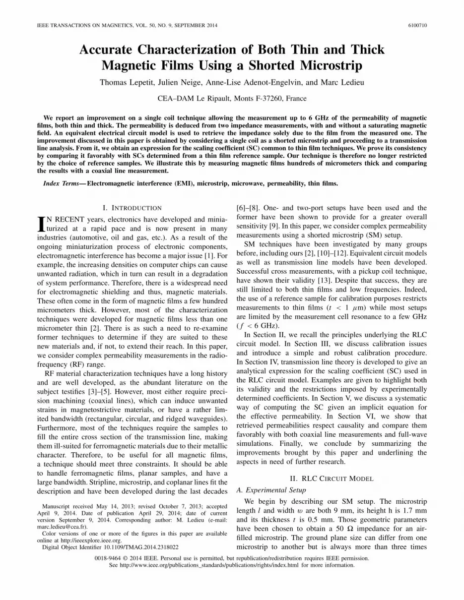
Fig. 1. (a) Coaxial cable (light blue) connects the VNA to a 50 � transition(dark blue) and from there to the microstrip (red); it is short-circuited to theground plane (gray) and the sample (green) is placed underneath; �1, �2,and �3 are the initial, intermediate, and final reference planes, respectively.(b) Picture of the experimental setup; the microstrip is gold-plated.

as wide as the strip itself. Our design is that of an openmicrostrip and, as such, cavity resonances, which occur inshielded microstrips, are not an issue. Fig. 1(a) and (b) showsa schematic of the measurement setup and a picture of theactual gold-plated microstrip, respectively.

The measured impedance of the SM is given by

Zm = Zc01 + S11

1 − S11(1)

where S11 is the scattering parameter and Zc0 is the emptymicrostrip characteristic impedance. It can be computedusing conformal mapping, for example, using Wheeler’s orHammerstad’s formula [14], [15]. In our setup, it is 50 �by design. Note that Zm , unlike Zc, depends via S11 on themicrostrip length.

B. Single Coil Technique

In order for this paper to be self-contained, a brief overviewof the RLC circuit model is provided. It is based on an analysisof the perturbation induced by a magnetic film in a coil. Here,the SM serves as a single loop coil, hence the name of thetechnique [2]. We assume that the x-component of the RFmagnetic field H can be written as

Hx = 1

K

i

w(2)

where i is the current and K is a dimensionless SC, specificto the geometry. Upon insertion of the film in the empty coil,the magnetic flux varies. Faraday’s law then gives the voltagedifference, which is assumed to vary sinusoidally in time.Considering the above expression of the magnetic field, theimpedance difference results and the relative permeability isgiven by

μr = 1 + K�Zw

jωμ0le(3)

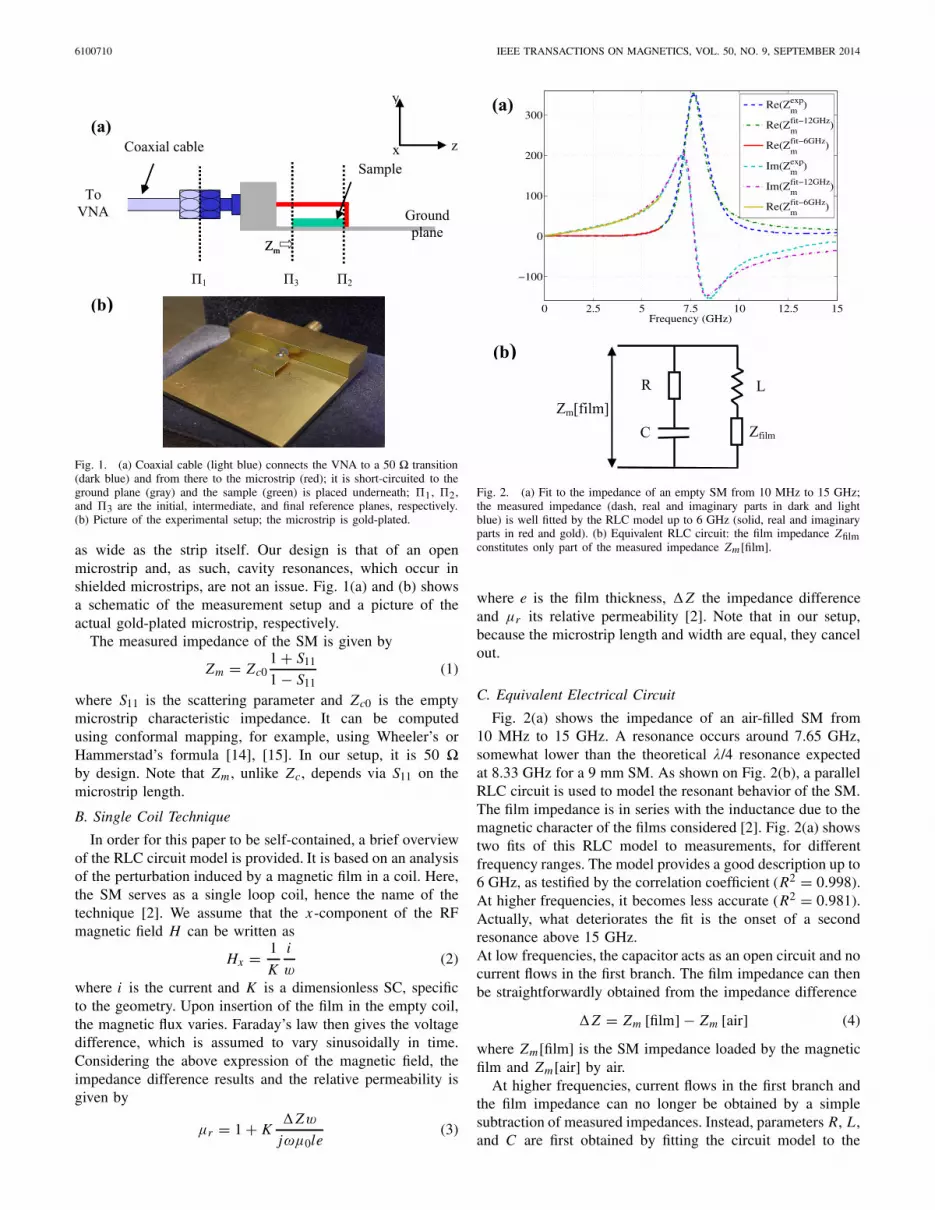
Fig. 2. (a) Fit to the impedance of an empty SM from 10 MHz to 15 GHz;the measured impedance (dash, real and imaginary parts in dark and lightblue) is well fitted by the RLC model up to 6 GHz (solid, real and imaginaryparts in red and gold). (b) Equivalent RLC circuit: the film impedance Zfilmconstitutes only part of the measured impedance Zm [film].

where e is the film thickness, �Z the impedance differenceand μr its relative permeability [2]. Note that in our setup,because the microstrip length and width are equal, they cancelout.

C. Equivalent Electrical Circuit

Fig. 2(a) shows the impedance of an air-filled SM from10 MHz to 15 GHz. A resonance occurs around 7.65 GHz,somewhat lower than the theoretical λ/4 resonance expectedat 8.33 GHz for a 9 mm SM. As shown on Fig. 2(b), a parallelRLC circuit is used to model the resonant behavior of the SM.The film impedance is in series with the inductance due to themagnetic character of the films considered [2]. Fig. 2(a) showstwo fits of this RLC model to measurements, for differentfrequency ranges. The model provides a good description up to6 GHz, as testified by the correlation coefficient (R2 = 0.998).At higher frequencies, it becomes less accurate (R2 = 0.981).Actually, what deteriorates the fit is the onset of a secondresonance above 15 GHz.At low frequencies, the capacitor acts as an open circuit and nocurrent flows in the first branch. The film impedance can thenbe straightforwardly obtained from the impedance difference

�Z = Zm [film] − Zm [air] (4)

where Zm[film] is the SM impedance loaded by the magneticfilm and Zm[air] by air.

At higher frequencies, current flows in the first branch andthe film impedance can no longer be obtained by a simplesubtraction of measured impedances. Instead, parameters R, L,and C are first obtained by fitting the circuit model to the

LEPETIT et al.: ACCURATE CHARACTERIZATION OF BOTH THIN AND THICK MAGNETIC FILMS 6100710

measured impedance of the air-filled SM [Fig. 2(a)]. Theextracted film impedance is then given by

Ze [film] = Zm [film] (R + 1/ jCω)

R + 1/ jCω − Zm [film]− j Lω. (5)

It would seem at first that the subtraction is no longernecessary because in theory Ze[air] = 0. However, it has beenfound very useful in practice to remove residual contributionsdue to both imperfect fitting and calibration

�Z = Ze [film] − Ze [air]. (6)

Note that this is strictly equivalent to the introduction of Za(ω)in series with Zfilm, as in [2].

For magnetic films deposited on a thick dielectric substrate,the same procedure is applied except that the second measure-ment is carried out with the SM loaded by the substrate and notair. Actually, it was found even better to load the SM with thesaturated magnetic film on its substrate. In this last case, filmpermeability is unity and all effects due to film permittivityare thus removed [16].

III. MICROSTRIP CALIBRATION

Commonly available calibration kits are designed for coax-ial connectors. The first step in any SM calibration procedure istherefore an open-short-load calibration. This brings the phasereference in the �1 plane [Fig. 1(a)].

A. Phase-Delay Calibration

Up to now, calibration has been done in two steps. First,the measured electrical delay between the �1 plane and theshorted-end of the microstrip is added. This brings the phasereference in the �2 plane. Finally, to move the phase referenceto the beginning of the microstrip, the theoretical propagationdelay due to the microstrip is subtracted. This brings the phasereference in the plane �3.

The obvious shortcoming of this calibration is that thetransition between the coaxial cable and the SM is assumedto be lossless and perfectly matched. This first point can beaddressed using a loss-estimation feature common to modernvector network analyzers (VNAs). In our experience, it isnot reliable over a wideband and is therefore discarded. Thesecond point can only be addressed by measuring knownreference standards (RSs). For a one-port setup, assumingthe transition is reciprocal, three of those are needed toaccount for directivity, source match, and reflection trackingerrors [5].

B. Full Calibration

The measured reflection coefficient can be expressed as afunction of the three error terms Ei and the actual reflectioncoefficient (Appendix A)

Sm11 = ED + ERT Sa

11

1 − ESMSa11

. (7)

Usual calibration kits operate with open (S11 = 1) and load(S11 = 0) standards besides a short (S11 = −1). As we donot have at our disposal such wideband standards, we choose

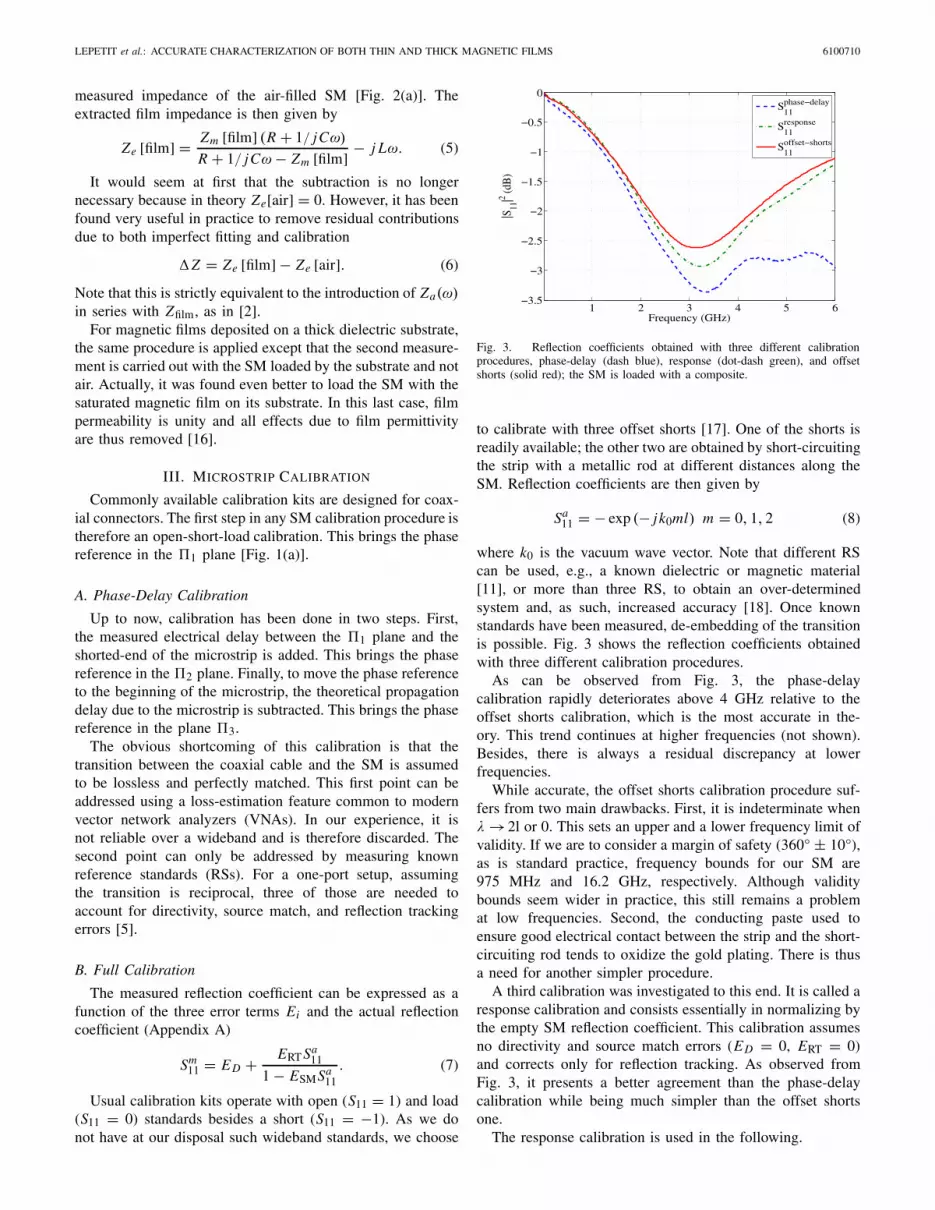
Fig. 3. Reflection coefficients obtained with three different calibrationprocedures, phase-delay (dash blue), response (dot-dash green), and offsetshorts (solid red); the SM is loaded with a composite.

to calibrate with three offset shorts [17]. One of the shorts isreadily available; the other two are obtained by short-circuitingthe strip with a metallic rod at different distances along theSM. Reflection coefficients are then given by

Sa11 = − exp (− jk0ml) m = 0, 1, 2 (8)

where k0 is the vacuum wave vector. Note that different RScan be used, e.g., a known dielectric or magnetic material[11], or more than three RS, to obtain an over-determinedsystem and, as such, increased accuracy [18]. Once knownstandards have been measured, de-embedding of the transitionis possible. Fig. 3 shows the reflection coefficients obtainedwith three different calibration procedures.

As can be observed from Fig. 3, the phase-delaycalibration rapidly deteriorates above 4 GHz relative to theoffset shorts calibration, which is the most accurate in the-ory. This trend continues at higher frequencies (not shown).Besides, there is always a residual discrepancy at lowerfrequencies.

While accurate, the offset shorts calibration procedure suf-fers from two main drawbacks. First, it is indeterminate whenλ →2l or 0. This sets an upper and a lower frequency limit ofvalidity. If we are to consider a margin of safety (360° ± 10°),as is standard practice, frequency bounds for our SM are975 MHz and 16.2 GHz, respectively. Although validitybounds seem wider in practice, this still remains a problemat low frequencies. Second, the conducting paste used toensure good electrical contact between the strip and the short-circuiting rod tends to oxidize the gold plating. There is thusa need for another simpler procedure.

A third calibration was investigated to this end. It is called aresponse calibration and consists essentially in normalizing bythe empty SM reflection coefficient. This calibration assumesno directivity and source match errors (ED = 0, ERT = 0)and corrects only for reflection tracking. As observed fromFig. 3, it presents a better agreement than the phase-delaycalibration while being much simpler than the offset shortsone.

The response calibration is used in the following.


IV. SCALING COEFFICIENT

A. Reference Sample

In the above RLC model, the SC K is assumed to be a con-stant, independent of frequency. It expresses the ratio betweenthe current density and the magnetic field and is considered tobe specific to a given SM. Up to now, it has been determinedby measuring a reference sample whose permeability is knowneither theoretically or via another technique (e.g., coaxial line).In practice, it is the result of the minimization, in the least-squares sense, of the following function:

g1(K

) = K(μmeasured

r − 1) − (

μreferencer − 1

). (9)

Until recently, the literature has supported the view thatthe SC is specific to a SM. To quote a review paper byLiu et al. [10] “K […] is independent of the thin film undertest.” However, [11] and [19] have underlined the necessityto go beyond this approximation. As shown below, a detailedanalysis of the transmission line model demonstrates that thisis an approximation only valid for very thin films.

B. Transmission Line Model

This model is framed within the quasi-static approximation.Its main hypothesis is that the microstrip first mode is trans-verse electromagnetic (TEM). This is not strictly true but itis a common assumption for such a transmission line [20].Following this, the propagation constant can be written

γ = jk0

√εeff

r μeffr . (10)

The permittivity and permeability are both effective becausethe sample does not fill the entire cross section and, as such,they reflect the properties of both the air surrounding thestrip and the film. Therefore, these effective parameters canonly be lower than the film’s. For a short-circuited microstrip,neglecting metallic losses on the strip and ground plane [20],the impedance is expressed as

Zm = Zc0

√μeff

r

εeffr

tanh

(jk0

√εeff

r μeffr l

). (11)

Note that, contrary to a widespread use [11], [13], we donot only consider the phase delay induced by the film but alsotake into account all multiple reflections, which occur within.In this way, we do not have to restrict ourselves to very thinsamples. That means this analysis, unlike previous ones, isnot perturbative (Appendix B). Furthermore, for low enoughfrequencies, we can develop the hyperbolic tangent to firstorder. Using this, the impedance difference is given by

�Z = Zc0 jk0l(μeff

r − 1)

(12)

where the first and second measurements are carried out asdescribed in Section II-C. Thus, the effective permeability canbe put in a form similar to (3)

μeffr = 1 + �ZC0

jωμ0lε0(13)

where C0 is the microstrip’s capacitance per unit length, whichcan be computed via conformal mapping with a precision of0.25% for an air-filled SM [20]. However, (13) does not givethe sample’s permeability.

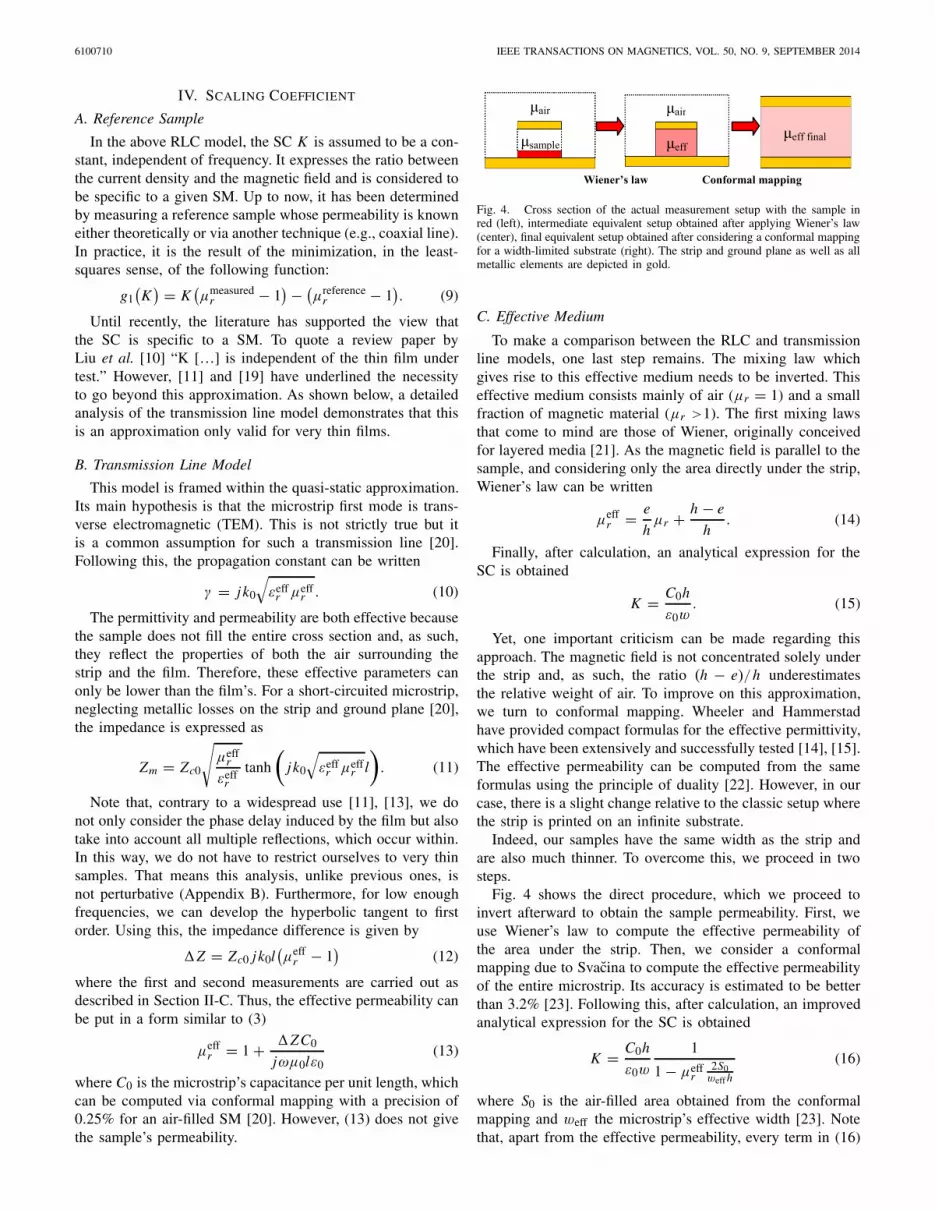
Fig. 4. Cross section of the actual measurement setup with the sample inred (left), intermediate equivalent setup obtained after applying Wiener’s law(center), final equivalent setup obtained after considering a conformal mappingfor a width-limited substrate (right). The strip and ground plane as well as allmetallic elements are depicted in gold.

C. Effective Medium

To make a comparison between the RLC and transmissionline models, one last step remains. The mixing law whichgives rise to this effective medium needs to be inverted. Thiseffective medium consists mainly of air (μr = 1) and a smallfraction of magnetic material (μr >1). The first mixing lawsthat come to mind are those of Wiener, originally conceivedfor layered media [21]. As the magnetic field is parallel to thesample, and considering only the area directly under the strip,Wiener’s law can be written

μeffr = e

hμr + h − e

h. (14)

Finally, after calculation, an analytical expression for theSC is obtained

K = C0h

ε0w. (15)

Yet, one important criticism can be made regarding thisapproach. The magnetic field is not concentrated solely underthe strip and, as such, the ratio (h − e)/h underestimatesthe relative weight of air. To improve on this approximation,we turn to conformal mapping. Wheeler and Hammerstadhave provided compact formulas for the effective permittivity,which have been extensively and successfully tested [14], [15].The effective permeability can be computed from the sameformulas using the principle of duality [22]. However, in ourcase, there is a slight change relative to the classic setup wherethe strip is printed on an infinite substrate.

Indeed, our samples have the same width as the strip andare also much thinner. To overcome this, we proceed in twosteps.

Fig. 4 shows the direct procedure, which we proceed toinvert afterward to obtain the sample permeability. First, weuse Wiener’s law to compute the effective permeability ofthe area under the strip. Then, we consider a conformalmapping due to Svacina to compute the effective permeabilityof the entire microstrip. Its accuracy is estimated to be betterthan 3.2% [23]. Following this, after calculation, an improvedanalytical expression for the SC is obtained

K = C0h

ε0w

1

1 − μeffr

2S0weff h

(16)

where S0 is the air-filled area obtained from the conformalmapping and weff the microstrip’s effective width [23]. Notethat, apart from the effective permeability, every term in (16)


is a real constant. However, precisely because of its presence,the SC is not. It is complex and, most of all, depends onthe material measured. Any dependence that the effectivepermeability has on frequency also finds its way into the SC.In short, in this mixing law the relative weights depend on thematerial. This goes contrary to the previous and widespreadinterpretation [10].

As a last refinement, we note that our microstrip’s thicknessis relatively important (t = 0.5 mm). To account for it, we usea correction for the effective permeability [24]. Note that, forthe previous expressions of the SC, we had already correctedthe capacitance C0 for the strip’s finite thickness [20]. All ofthis considered, after calculation, the expression for the SCbecomes

K = C0h

ε0w

1

1 − μeffr

(2S0

weff h + t4.6

√wh

) . (17)

This is the expression we use in the following.

D. Dynamic Corrections to Wiener’s Law

It is possible to improve upon the first step, Wiener’s law, byconsidering dynamic corrections, as was done by Rytov [25].The effective permeability is then modified by a factor

�μeffr = 1

12

(k0e (h − e)

h

)2

εW‖r εW⊥

rμr − 1/εr

(μr − 1)−1 (18)

where the W || and W⊥ superscripts refer to parallel andperpendicular Wiener’s laws [21]. Notice that beyond thequasi-static approximation, permittivity and permeability areno longer decoupled. An estimation of the permittivity istherefore needed.

For nonmetallic films, e.g., composites (Fig. 7), we cansafely consider permittivities below 100. In the worst casescenario, at the highest frequency (6 GHz), for a thick film(100 μm), and for a permeability of 15, this correction onlyamounts to a few hundredths and is thus negligible. For metal-lic films, e.g., ferromagnetics (Fig. 5), we can safely considerconductivities below 107 S · m−1. At the highest frequency(6 GHz) and for a permeability of 1000, the correctionbecomes superior to 100 (10%) for films that are morethan 1.6 μm thick. Actually, (18) is only valid provided thecorrection is small. For metallic films, it means the thicknessshould be smaller than the skin depth [25].

This small correction factor is neglected in the following.

E. Examples: From Thin to Thick Films

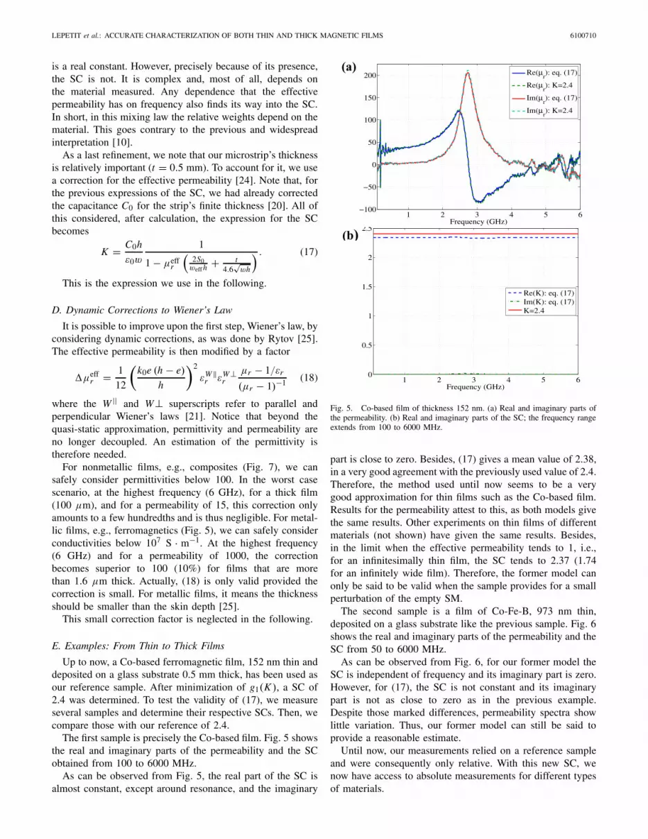
Up to now, a Co-based ferromagnetic film, 152 nm thin anddeposited on a glass substrate 0.5 mm thick, has been used asour reference sample. After minimization of g1(K ), a SC of2.4 was determined. To test the validity of (17), we measureseveral samples and determine their respective SCs. Then, wecompare those with our reference of 2.4.

The first sample is precisely the Co-based film. Fig. 5 showsthe real and imaginary parts of the permeability and the SCobtained from 100 to 6000 MHz.

As can be observed from Fig. 5, the real part of the SC isalmost constant, except around resonance, and the imaginary

Fig. 5. Co-based film of thickness 152 nm. (a) Real and imaginary parts ofthe permeability. (b) Real and imaginary parts of the SC; the frequency rangeextends from 100 to 6000 MHz.

part is close to zero. Besides, (17) gives a mean value of 2.38,in a very good agreement with the previously used value of 2.4.Therefore, the method used until now seems to be a verygood approximation for thin films such as the Co-based film.Results for the permeability attest to this, as both models givethe same results. Other experiments on thin films of differentmaterials (not shown) have given the same results. Besides,in the limit when the effective permeability tends to 1, i.e.,for an infinitesimally thin film, the SC tends to 2.37 (1.74for an infinitely wide film). Therefore, the former model canonly be said to be valid when the sample provides for a smallperturbation of the empty SM.

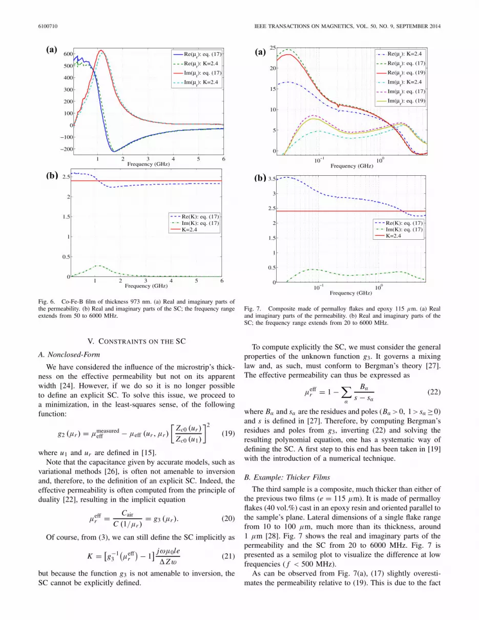
The second sample is a film of Co-Fe-B, 973 nm thin,deposited on a glass substrate like the previous sample. Fig. 6shows the real and imaginary parts of the permeability and theSC from 50 to 6000 MHz.

As can be observed from Fig. 6, for our former model theSC is independent of frequency and its imaginary part is zero.However, for (17), the SC is not constant and its imaginarypart is not as close to zero as in the previous example.Despite those marked differences, permeability spectra showlittle variation. Thus, our former model can still be said toprovide a reasonable estimate.

Until now, our measurements relied on a reference sampleand were consequently only relative. With this new SC, wenow have access to absolute measurements for different typesof materials.


Fig. 6. Co-Fe-B film of thickness 973 nm. (a) Real and imaginary parts ofthe permeability. (b) Real and imaginary parts of the SC; the frequency rangeextends from 50 to 6000 MHz.

V. CONSTRAINTS ON THE SC

A. Nonclosed-Form

We have considered the influence of the microstrip’s thick-ness on the effective permeability but not on its apparentwidth [24]. However, if we do so it is no longer possibleto define an explicit SC. To solve this issue, we proceed toa minimization, in the least-squares sense, of the followingfunction:

g2 (μr ) = μmeasuredeff − μeff (ur , μr )

[Zc0 (ur )

Zc0 (u1)

]2

(19)

where u1 and ur are defined in [15].Note that the capacitance given by accurate models, such as

variational methods [26], is often not amenable to inversionand, therefore, to the definition of an explicit SC. Indeed, theeffective permeability is often computed from the principle ofduality [22], resulting in the implicit equation

μeffr = Cair

C (1/μr )= g3 (μr ). (20)

Of course, from (3), we can still define the SC implicitly as

K = [g−1

3

(μeff

r

) − 1] jωμ0le

�Zw(21)

but because the function g3 is not amenable to inversion, theSC cannot be explicitly defined.

Fig. 7. Composite made of permalloy flakes and epoxy 115 μm. (a) Realand imaginary parts of the permeability. (b) Real and imaginary parts of theSC; the frequency range extends from 20 to 6000 MHz.

To compute explicitly the SC, we must consider the generalproperties of the unknown function g3. It governs a mixinglaw and, as such, must conform to Bergman’s theory [27].The effective permeability can thus be expressed as

μeffr = 1 −

∑

α

Bα

s − sα(22)

where Bα and sα are the residues and poles (Bα >0, 1>sα ≥0)and s is defined in [27]. Therefore, by computing Bergman’sresidues and poles from g3, inverting (22) and solving theresulting polynomial equation, one has a systematic way ofdefining the SC. A first step to this end has been taken in [19]with the introduction of a numerical technique.

B. Example: Thicker Films

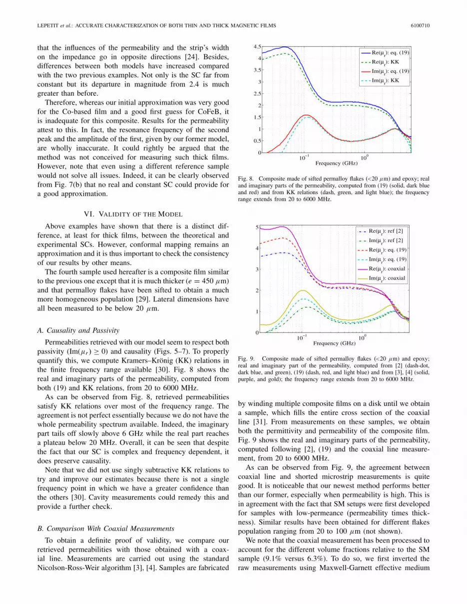
The third sample is a composite, much thicker than either ofthe previous two films (e = 115 μm). It is made of permalloyflakes (40 vol.%) cast in an epoxy resin and oriented parallel tothe sample’s plane. Lateral dimensions of a single flake rangefrom 10 to 100 μm, much more than its thickness, around1 μm [28]. Fig. 7 shows the real and imaginary parts of thepermeability and the SC from 20 to 6000 MHz. Fig. 7 ispresented as a semilog plot to visualize the difference at lowfrequencies ( f < 500 MHz).

As can be observed from Fig. 7(a), (17) slightly overesti-mates the permeability relative to (19). This is due to the fact


that the influences of the permeability and the strip’s widthon the impedance go in opposite directions [24]. Besides,differences between both models have increased comparedwith the two previous examples. Not only is the SC far fromconstant but its departure in magnitude from 2.4 is muchgreater than before.

Therefore, whereas our initial approximation was very goodfor the Co-based film and a good first guess for CoFeB, itis inadequate for this composite. Results for the permeabilityattest to this. In fact, the resonance frequency of the secondpeak and the amplitude of the first, given by our former model,are wholly inaccurate. It could rightly be argued that themethod was not conceived for measuring such thick films.However, note that even using a different reference samplewould not solve all issues. Indeed, it can be clearly observedfrom Fig. 7(b) that no real and constant SC could provide fora good approximation.

VI. VALIDITY OF THE MODEL

Above examples have shown that there is a distinct dif-ference, at least for thick films, between the theoretical andexperimental SCs. However, conformal mapping remains anapproximation and it is thus important to check the consistencyof our results by other means.

The fourth sample used hereafter is a composite film similarto the previous one except that it is much thicker (e = 450 μm)and that permalloy flakes have been sifted to obtain a muchmore homogeneous population [29]. Lateral dimensions haveall been measured to be below 20 μm.

A. Causality and Passivity

Permeabilities retrieved with our model seem to respect bothpassivity (Im(μr ) ≥ 0) and causality (Figs. 5–7). To properlyquantify this, we compute Kramers–Krönig (KK) relations inthe finite frequency range available [30]. Fig. 8 shows thereal and imaginary parts of the permeability, computed fromboth (19) and KK relations, from 20 to 6000 MHz.

As can be observed from Fig. 8, retrieved permeabilitiessatisfy KK relations over most of the frequency range. Theagreement is not perfect essentially because we do not have thewhole permeability spectrum available. Indeed, the imaginarypart tails off slowly above 6 GHz while the real part reachesa plateau below 20 MHz. Overall, it can be seen that despitethe fact that our SC is complex and frequency dependent, itdoes preserve causality.

Note that we did not use singly subtractive KK relations totry and improve our estimates because there is not a singlefrequency point in which we have a greater confidence thanthe others [30]. Cavity measurements could remedy this andprovide a further check.

B. Comparison With Coaxial Measurements

To obtain a definite proof of validity, we compare ourretrieved permeabilities with those obtained with a coax-ial line. Measurements are carried out using the standardNicolson-Ross-Weir algorithm [3], [4]. Samples are fabricated

Fig. 8. Composite made of sifted permalloy flakes (<20 μm) and epoxy; realand imaginary parts of the permeability, computed from (19) (solid, dark blueand red) and from KK relations (dash, green, and light blue); the frequencyrange extends from 20 to 6000 MHz.

Fig. 9. Composite made of sifted permalloy flakes (<20 μm) and epoxy;real and imaginary part of the permeability, computed from [2] (dash-dot,dark blue, and green), (19) (dash, red, and light blue) and from [3], [4] (solid,purple, and gold); the frequency range extends from 20 to 6000 MHz.

by winding multiple composite films on a disk until we obtaina sample, which fills the entire cross section of the coaxialline [31]. From measurements on these samples, we obtainboth the permittivity and permeability of the composite film.Fig. 9 shows the real and imaginary parts of the permeability,computed following [2], (19) and the coaxial line measure-ment, from 20 to 6000 MHz.

As can be observed from Fig. 9, the agreement betweencoaxial line and shorted microstrip measurements is quitegood. It is noticeable that our newest method performs betterthan our former, especially when permeability is high. This isin agreement with the fact that SM setups were first developedfor samples with low-permeance (permeability times thick-ness). Similar results have been obtained for different flakespopulation ranging from 20 to 100 μm (not shown).

We note that the coaxial measurement has been processed toaccount for the different volume fractions relative to the SMsample (9.1% versus 6.3%). To do so, we first inverted theraw measurements using Maxwell-Garnett effective medium


theory [21]

μeffr − 1 = fc (μr − 1)

1 + N (1 − fc) (μr − 1)� fc (μr − 1) (23)

where fc is the volume fraction of the coaxial sample andN the flakes demagnetizing factor (N = 0.01). We thusobtained the intrinsic permeability of flakes, which we thenused to compute the effective permeability of the compositewith the appropriate volume fraction. This process is possiblebecause we work with low volume fractions ( f < 10%) forwhich Maxwell–Garnett theory is known to be accurate [21].

As a last comment, we note that this comparison withcoaxial measurements was possible because our compositedoes not show any pronounced magnetostrictive effects. Fora ferromagnetic thin film, a direct comparison is not possiblealthough other methods have been investigated [32].

C. Comparison With Full-Wave Simulations

So far, we have proved the validity of our model for thespecific samples that we measured. The question remains asto its broader limits.

The main hypothesis in our model is the existence of a TEMmode. While it is reasonable at low frequencies, it deterioratesas frequency increases. We are therefore left with the question,how big is the discrepancy at the maximum frequency (in ourcase 6 GHz)? Departure from the TEM mode can be shown tobe due, in a first approximation, to propagation of unwantedsubstrate modes [33]. The cutoff frequency of the lowest-ordermode can thus be considered as a fundamental limit. However,it depends on the material being measured. The frequency limitis therefore material dependent and cannot be asserted onceand for all for a given setup. To obtain a practical limit, wetherefore define a permeance limit and not a frequency one.It is to be understood as follows, all materials having a lowerpermeance than this limit can be reliably measured using ourmodel.

To compute this limit, we proceed to full-wave simulationsof our setup with a commercial finite-element software (AnsoftHFSS v.11). We consider two different materials with the samefrequency-independent permeability (μr = 5, tanδμ = 0.2),differing permittivities (εr = 12 and 5, tanδε = 0.02) and athickness varying from 100 to 800 μm. We compute scatteringparameters S11, both when the material is saturated and whenit is not, and use our model to estimate the permeability. Notethat to forego the RLC fitting procedure we use the methodfrom [34]. Fig. 10 shows the real and imaginary parts ofpermeability retrieved from simulations, at the frequency of6 GHz, as a function of thickness, and for both materials.

As can be observed from Fig. 10, retrieved permeabilitiesagree well with the simulated ones up to 0.5 mm (less than 9%error). Above this limit, the discrepancy grows very quicklywith film thickness. The permeance limit of our setup cantherefore be taken to be 2.5 mm. All materials with a lowerpermeance can thus be measured from 10 MHz to 6 GHz withour setup.

The discrepancy can be seen to grow more quickly forthe highest permittivity material. That is consistent with theappearance of substrate modes as explained above. However,

Fig. 10. Frequency-independent magnetic materials (μr = 5 − j); retrievedreal and imaginary parts of the permeability, for a permittivity of 12 (dashand dash-dot, dark blue, and green) and for a permittivity of 5 (dash anddash-dot, red, and light blue) for a film thickness ranging from 0.1 to0.8 mm; simulated real and imaginary parts of the permeability are also shownfor comparison (dash and dash-dot, black).

it also means that our permeance limit is only valid formaterials with a permittivity lower or equal to 12. Thispermeance limit should therefore be used knowingly and withcaution.

Note that this limit is also setup dependent in the sense thatit is influenced by the sample width. Setups, which rely onsamples much wider than the strip therefore have different,and lower, permeance limits [11].

VII. CONCLUSION

In this paper, we have shown that a technique for mea-suring thin magnetic films with a SM can be improved. Wehave proceeded in four steps. First, we derived an analyticalexpression for a coefficient, which was determined experi-mentally up to now. Then, we proved experimentally thatthe two are consistent for very thin films. Afterward, weused this new expression of the coefficient to measure thickfilms and highlight the fact that experimentally determinedcoefficients are not suited to such films. Finally, we determinedthe limits of our setup and expressed those under the formof a permeance limit (μr e < 2.5 mm). To conclude, wenow have access to absolute measurements of both thin andthick films, which is especially valuable for high-permeancefilms. In the future, a further improvement might be achievedby considering techniques, variational or numerical, whichaccount for the full detail of the microstrip geometry.

APPENDIX

A. Vector Calibration

The transition between the coaxial cable and the SM canbe modeled as a two-port network. Within this framework, theactual reflection coefficient is given by

Sm11 = St

11 + St21St

12 Sa11

1 − St22Sa

11(A1)


where the t superscript refers to the transition. Error termsintroduced in Section III-B are thus simply related to thistwo-port network. There are only three of those due to thedevice reciprocity (S21 = S12)

ED = St11, ESM = St

22, ERT = St21St

12. (A2)

To de-embed the reflection coefficient, errors can be com-puted with the following matrix equation:⎛

⎝ED

ERT − ED ESMESM

⎞

⎠ =⎛

⎜⎝

1 Sr111 Sr1

11 Sm111

1 Sr211 Sr2

11 Sm211

1 Sr311 Sr3

11 Sm311

⎞

⎟⎠

−1 ⎛

⎜⎝

Sm111

Sm211

Sm311

⎞

⎟⎠ (A3)

where the r superscript refers to the RS. It appears that whenthe phase difference between two different offset shorts is toosmall, the matrix is ill-conditioned and the procedure is thushighly sensitive to noise.

Once error terms are computed, the calibrated reflectioncoefficient is obtained

Sc11 = Sm

11 − ED

ESM(Sm

11 − ED) + ERT

. (A4)

If more than three RS are available for calibration, they canbe directly incorporated in (A3). Note that it is also possibleto include multiple measurements of the same RS to considerrandom errors due to connector repeatability [18].

B. Perturbative Versus Low-Frequency Approximations

There is a difference between a perturbative approximationand a low-frequency-one.

The reflection scattering parameter for a SM is given by

S11 = Zeff tanh (γeff l) − 1

Zeff tanh (γeff l) + 1(B1)

where Zeff and γeff are the effective impedance and propaga-tion constant, respectively. It can be put in a different form

S11 = e+γeff l (Zeff − 1) − e−γeff l (Zeff + 1)

e+γeff l (Zeff + 1) − e−γeff l (Zeff − 1). (B2)

In a perturbative approximation, the effective impedance isclose to unity and the reflection scattering parameter is then

S11 = −e−2γeff l (B3)

which is precisely the expression used in [11] and [13].In a low-frequency approximation, the argument of the

hyperbolic tangent is small and, to lowest order in the Taylorseries, the reflection scattering parameter is then

S11 = Zeffγeff l − 1

Zeffγeff l + 1. (B4)

Therefore, these two approximations are distinct. Note that thefirst one does necessitate the assumption of an almost emptymicrostrip and cannot be used, as such, to measure thick films.

ACKNOWLEDGMENT

The authors would like to thank S. Dubourg for providingthe sample of CoFeB. The work of J. Neige was supported bythe Direction Générale de l’Armement.

REFERENCES

[1] D. D. L. Chung, “Electromagnetic interference shielding effective-ness of carbon materials,” Carbon, vol. 39, no. 2, pp. 279–285,2001.

[2] D. Pain, M. Ledieu, O. Acher, A.-L. Adenot, and F. Duverger, “Animproved permeameter for thin film measurements up to 6 GHz,” J. Appl.Phys., vol. 85, no. 8, pp. 5151–5153, 1999.

[3] A. M. Nicolson and G. F. Ross, “Measurement of the intrinsic propertiesof materials by time-domain techniques,” IEEE Trans. Instrum. Meas.,vol. 19, no. 4, pp. 377–382, Nov. 1970.

[4] W. B. Weir, “Automatic measurement of complex dielectric constantand permeability at microwave frequencies,” Proc. IEEE, vol. 62, no. 1,pp. 33–36, Jan. 1974.

[5] L. F. Chen, C. K. Ong, C. P. Neo, V. V. Varadan, and V. K. Varadan,Microwave Electronics: Measurement and Materials Characterization.Hoboken, NJ, USA: Wiley, 2004, ch. 2.

[6] M. Yamaguchi, S. Yabukami, and K. I. Arai, “A new 1 MHz-2 GHzpermeance meter for metallic thin films,” IEEE Trans. Magn., vol. 33,no. 5, pp. 3619–3621, Sep. 1997.

[7] P. Quéffélec, S. Mallégol, and M. Le Floc’h, “Automatic measurementof complex tensorial permeability of magnetized materials in a widemicrowave frequency range,” IEEE Trans. Microw. Theory Techn.,vol. 50, no. 9, pp. 2128–2134, Sep. 2002.

[8] C. Bilzer, T. Devolder, P. Crozat, C. Chappert, and S. Cardoso, “Vectornetwork analyzer ferromagnetic resonance of thin films on coplanarwaveguides: Comparison of different evaluation methods,” J. Appl.Phys., vol. 101, no. 7, pp. 074505-1–074505-5, 2007.

[9] Y. Wu, Z. Tang, Y. Xu, and B. Zhang, “Measure the complex permeabil-ity of ferromagnetic thin films: Comparison shorted microstrip methodwith microstrip transmission method,” PIER Lett., vol. 11, pp. 173–181,2009.

[10] Y. Liu, L. Chen, C. Y. Tan, H. J. Liu, and C. K. Ong, “Broadbandcomplex permeability characterization of magnetic thin films usingshorted microstrip transmission-line perturbation,” Rev. Sci. Instrum.,vol. 76, no. 6, p. 063911, 2005.

[11] S. N. Starostenko, K. N. Rozanov, and A. V. Osipov, “A broadbandmethod to measure magnetic spectra of thin films,” J. Appl. Phys.,vol. 103, no. 7, p. 07E914, 2008.

[12] V. Bekker, K. Seemann, and H. Leiste, “A new strip line broad-bandmeasurement evaluation for determining the complex permeability ofthin ferromagnetic films,” J. Magn. Magn. Mater., vol. 270, no. 3,pp. 327–332, 2004.

[13] M. Yamaguchi, O. Acher, Y. Miyazawa, K. I. Arai, and M. Ledieu,“Cross measurements of thin-film permeability up to UHF range,”J. Magn. Magn. Mater., vols. 242–245, pp. 970–972, Apr. 2002.

[14] H. A. Wheeler, “Transmission-line properties of a strip on a dielectricsheet on a plane,” IEEE Trans. Microw. Theory Techn., vol. 25, no. 8,pp. 631–647, Aug. 1977.

[15] E. Hammerstad and Ø. Jensen, “Accurate models for microstripcomputer-aided design,” in IEEE MTT-S Int. Microwave Symp. Dig.,Washington, DC, USA, May 1980, pp. 407–409.

[16] P.-M. Jacquart and L. Roux, “Influence of the electrical resistivity ofa ferromagnetic thin film on its permeability measurement performedwith a permeameter,” J. Magn. Magn. Mater., vol. 281, no. 1, pp. 82–91,2004.

[17] G. W. Hanson, J. M. Grimm, and D. P. Nyquist, “An improved de-embedding technique for the measurement of the complex constitutiveparameters of materials using a stripline field applicator,” IEEE Trans.Instrum. Meas., vol. 42, no. 3, pp. 740–745, Jun. 1993.

[18] R. B. Marks, “A multiline method of network analyzer calibration,”IEEE Trans. Microw. Theory Techn., vol. 39, no. 7, pp. 1205–1215,Jul. 1991.

[19] T. Sebastian, S. A. Clavijo, and R. E. Diaz, “Improved accuracy thin filmpermeability extraction for a microstrip permeameter,” J. Appl. Phys.,vol. 113, no. 3, p. 033906, 2013.

[20] R. E. Collin, “Transmission lines and waveguides,” in Foundations forMicrowave Engineering, 2nd ed. Hoboken, NJ, USA: Wiley, 2001, ch. 3,pp. 130–157.

[21] A. Sihvola, “Difficulties and uncertainties in classical mixing,” inElectromagnetic Mixing Formulas and Applications. London, U.K.: IEE,1999, ch. 8, pp. 151–152.

[22] R. A. Pucel and D. J. Massé, “Microstrip propagation on magneticsubstrates—Part I: Design theory,” IEEE Trans. Microw. Theory Techn.,vol. 20, no. 5, pp. 304–308, May 1972.


[23] J. Svacina, “Analytical models of width-limited microstrip lines,”Microw. Opt. Technol. Lett., vol. 36, no. 1, pp. 63–65, 2003.

[24] I. J. Bahl and R. Garg, “Simple and accurate formulas for a microstripwith finite strip thickness,” Proc. IEEE, vol. 65, no. 11, pp. 1611–1612,Nov. 1977.

[25] S. M. Rytov, “Electromagnetic properties of a finely stratified medium,”Sov. Phys. JETP, vol. 2, pp. 466–475, 1956.

[26] R. E. Collin, “Transmission lines,” in Field Theory of Guided Waves,2nd ed. Piscataway, NJ, USA: IEEE Press, 1990, ch. 4, pp. 273–285.

[27] D. J. Bergman, “The dielectric constant of a composite material—Aproblem in classical physics,” Phys. Rep., vol. 43, no. 9, pp. 377–407,1978.

[28] J. Neige, T. Lepetit, A.-L. Adenot-Engelvin, N. Malléjac,A. Thiaville, and N. Vukadinovic, “Microwave permeability ofFeNiMo flakes-polymer composites with and without an applied staticmagnetic field,” IEEE Trans. Magn., vol. 49, no. 3, pp. 1005–1008,Mar. 2013.

[29] J. Neige, T. Lepetit, N. Malléjac, A.-L. Adenot-Engelvin, A. Thiaville,and N. Vukadinovic, “Evidence of an embedded vortex translation modein flake-shaped ferromagnetic particle composites,” Appl. Phys. Lett.,vol. 102, no. 24, pp. 242401-1–242401-4, 2013.

[30] V. Lucarini, J. J. Saarinen, K.-E. Peiponen, and E. M. Vartiainen,“Kramers-Kronig relations and sum rules in linear optics,” in Kramers-Kronig Relations in Optical Materials Research. Berlin, Germany:Springer-Verlag, 2005, ch. 4, pp. 44–48.

[31] O. Acher, J. L. Vermeulen, P. M. Jacquart, J. M. Fontaine, and P. Baclet,“Permeability measurement on ferromagnetic thin films from 50 MHzup to 18 GHz,” J. Magn. Magn. Mater., vol. 136, no. 3, pp. 269–278,1994.

[32] I. T. Iakubov et al., “A contribution from the magnetoelastic effect tomeasured microwave permeability of thin ferromagnetic films,” J. Magn.Magn. Mater., vol. 324, no. 21, pp. 3385–3388, 2012.

[33] A. A. Oliner, “Types and basic properties of leaky modes in microwaveand millimeter-wave integrated circuits,” IEICE Trans. Electron.,vol. E83-C, no. 5, pp. 675–686, 2000.

[34] E. Moraitakis, L. Kompotiatis, M. Pissas, and D. Niarchos, “Perme-ability measurements of permalloy films with a broad band striplinetechnique,” J. Magn. Magn. Mater., vol. 222, nos. 1–2, pp. 168–174,2000.

Thomas Lepetit was born in Paris, France, in 1984. He received the Engineerdegree from Telecom Physique Strasbourg, Illkirch-Graffenstaden, France;the M.S. degree in photonics from the University of Strasbourg, Strasbourg,France, in 2006; and the Ph.D. degree in electrical engineering from theUniversity of Orsay, Orsay, France, in 2010.

He was with Institut Langevin ESPCI, Paris, in 2010, and since 2011, hasbeen with CEA, Tours, France, as a Post-Doctoral Researcher. His researchinterests include microwave materials characterization, homogenization ofcomposites and metamaterials, bianisotropic and chiral materials, SAR, arraysignal processing, and computational electromagnetics, in particular, photoniccrystals.

Julien Neige was born in France in 1987. He received the Engineer degree inadvanced materials from the Engineering School of Limoges, University ofLimoges, Limoges, France, and the M.S. degree in ceramics materials fromthe University of Limoges in 2010. He is currently pursuing the Ph.D. degreein electromagnetic engineering with CEA, DAM Le Ripault, Monts, France.

His research interests include electromagnetic wave propagation throughcomplex systems, ordered and disordered flakes-polymer media, and modelingand the characterization of materials.

Anne-Lise Adenot-Engelvin was born in France in 1974. She received theEngineer and M.S. degrees from the Engineering School in Chemistry andPhysics of Bordeaux, Bordeaux, France, in 1997, and the Ph.D. degree in2000, dealing with the dielectric and magnetic properties of heterogeneousmedia.

She has been with CEA le Ripault, Monts, France, since 2001. Her researchinterests include ferromagnetic microwires, applications of ferromagneticcomposites in microwave devices, and magnetic properties of ferromagneticflakes.

Marc Ledieu was born in France in 1973. He received the Engineer degreefrom the ESEO Electrical Engineering School of Angers, Angers, France, in1996, and the Ph.D. degree from the University of Tours, Tours, France, in2005.

He has been with CEA, Tours, since 1998, as a Research Engineer. Hisresearch interests include microwave materials characterization and metama-terials.

Documents

Accurate Characterization of both Thin and Thick Magnetic FilmsUsing a Shorted Microstrip